digital signal processing using matlab- michael weeks
DESCRIPTION
Digital Signal Processing using MATLAB Michael Weeks.TRANSCRIPT

DIGITAL SIGNAL PROCESSING
DIGITAL SIGNAL PROCESSINGUsing MATLAB®
and Wavelets
Michael Weeks
Shelving: Engineering / Computer Science ISBN: 0-9778582-0-0Level: Intermediate to Advanced U.S. $69.95 / Canada $85.50
All trademarks and service marks are the property of their respective owners.Cover design: Tyler Creative
INFINITY SCIENCE PRESS11 Leavitt StreetHingham, MA 02043(781) 740-4487(781) 740-1677 FAXinfo@infi nitysciencepress.comwww.infi nitysciencepress.com
Using MATLAB
® and W
avelets
E L E C T R I C A L E N G I N E E R I N G S E R I E S
DIGITAL SIGNAL PROCESSINGUsing MATLAB® and Wavelets
Michael Weeks
Although DSP has long been considered an EE topic, recent developments have also generated sig-nifi cant interest from the computer science community. DSP applications in the consumer market, such as bioinformatics, the MP3 audio format, and MPEG-based cable/satellite television have fueled a desire to understand this technology outside of hardware circles.
Designed for upper division engineering and computer science students as well as practicing engineers, Digital Signal Processing Using MATLAB and Wavelets emphasizes the practical applications of signal processing. Over 100 MATLAB examples and wavelet techniques provide the latest applications of DSP, including image processing, games, fi lters, transforms, networking, parallel processing, and sound.
The book also provides the mathematical processes and techniques needed to ensure an understand-ing of DSP theory. Designed to be incremental in diffi culty, the book will benefi t readers who are unfamiliar with complex mathematical topics or those limited in programming experience. Beginning with an introduction to MATLAB programming, it moves through fi lters, sinusoids, sampling, the Fou-rier transform, the z-transform and other key topics. An entire chapter is dedicated to the discussion of wavelets and their applications. A CD-ROM (platform independent) accompanies the book and contains source code, projects for each chapter, and the fi gures contained in the book.
FEATURES: Contains over 100 short examples in MATLAB used
throughout the book Includes an entire chapter on the wavelet transform Designed for the reader who does not have extensive
math and programming experience Accompanied by a CD-ROM containing MATLAB
examples, source code, projects, and fi gures from the book
Contains modern applications of DSP and MATLAB project ideas
ABOUT THE AUTHOR:Michael Weeks is an associate professor at Georgia State University where he teaches courses in Digital Signal Processing. He holds a PhD in computer engineering from the University of Louisiana at Lafayette and has authored or co-authored numerous journal and conference papers.
WEEKS
BRIEF TABLE OF CONTENTS:1. Introduction. 2. MATLAB. 3. Filters. 4. Sinusoids. 5. Sampling. 6. The Fourier Transform. 7. The Number e. 8. The z-Transform. 9. The Wavelet Transform 10. Applications. Appendix A. Constants and Variables. B. Equations. C. DSP Project Ideas. D. About the CD. Answers. Glossary. Index.
weeks_DSP.indd 1weeks_DSP.indd 1 8/11/06 1:15:29 PM8/11/06 1:15:29 PM

Digital Signal ProcessingUsing MATLAB r© and Wavelets

License, Disclaimer of Liability, and Limited Warranty
The CD-ROM that accompanies this book may only be used on a single PC. Thislicense does not permit its use on the Internet or on a network (of any kind). Bypurchasing or using this book/CD-ROM package (the “Work”), you agree that thislicense grants permission to use the products contained herein, but does not giveyou the right of ownership to any of the textual content in the book or ownership toany of the information or products contained on the CD-ROM. Use of third partysoftware contained herein is limited to and subject to licensing terms for the respec-tive products, and permission must be obtained from the publisher or the owner ofthe software in order to reproduce or network any portion of the textual materialor software (in any media) that is contained in the Work.
Infinity Science Press LLC (“ISP” or “the Publisher”) and anyone involvedin the creation, writing or production of the accompanying algorithms, code, orcomputer programs (“the software”) or any of the third party software contained onthe CD-ROM or any of the textual material in the book, cannot and do not warrantthe performance or results that might be obtained by using the software or contentsof the book. The authors, developers, and the publisher have used their best ef-forts to insure the accuracy and functionality of the textual material and programscontained in this package; we, however, make no warranty of any kind, express orimplied, regarding the performance of these contents or programs. The Work is sold“as is” without warranty (except for defective materials used in manufacturing thedisc or due to faulty workmanship);
The authors, developers, and the publisher of any third party software, and anyoneinvolved in the composition, production, and manufacturing of this work will not beliable for damages of any kind arising out of the use of (or the inability to use) thealgorithms, source code, computer programs, or textual material contained in thispublication. This includes, but is not limited to, loss of revenue or profit, or otherincidental, physical, or consequential damages arising out of the use of this Work.
The sole remedy in the event of a claim of any kind is expressly limited to replace-ment of the book and/or the CD-ROM, and only at the discretion of the Publisher.
The use of “implied warranty” and certain “exclusions” vary from state to state,and might not apply to the purchaser of this product.

Digital Signal ProcessingUsing MATLAB r© and Wavelets
Michael WeeksGeorgia State University
Infinity Science Press LLC
Hingham, Massachusetts

Copyright 2007 by Infinity Science Press LLC
All rights reserved.
This publication, portions of it, or any accompanying software may not be reproduced in any way, stored in
a retrieval system of any type, or transmitted by any means or media, electronic or mechanical, including,
but not limited to, photocopy, recording, Internet postings or scanning, without prior permission in writing
from the publisher.
Publisher: David F. Pallai
Infinity Science Press LLC
11 Leavitt StreetHingham, MA 02043Tel. 877-266-5796 (toll free)Fax 781-740-1677info@infinitysciencepress.comwww.infinitysciencepress.com
This book is printed on acid-free paper.
Michael Weeks. Digital Signal Processing Using MATLAB and Wavelets.ISBN: 0-9778582-0-0
The publisher recognizes and respects all marks used by companies, manufacturers, and developers as ameans to distinguish their products. All brand names and product names mentioned in this book are trade-marks or service marks of their respective companies. Any omission or misuse (of any kind) of service marksor trademarks, etc. is not an attempt to infringe on the property of others.
Library of Congress Cataloging-in-Publication Data
Weeks, Michael.Digital signal processing using MATLAB and Wavelets / Michael Weeks.
p. cm.Includes index.ISBN 0-9778582-0-0 (hardcover with cd-rom : alk. paper)
1. Signal processing–Digital techniques–Mathematics. 2. MATLAB. 3. Wavelets (Mathematics) I.Title.
TK5102.9.W433 2006621.382’2–dc22
2006021318
6 7 8 9 5 4 3 2 1
Our titles are available for adoption, license or bulk purchase by institutions, corporations, etc. For ad-ditional information, please contact the Customer Service Dept. at 877-266-5796 (toll free).
Requests for replacement of a defective CD-ROM must be accompanied by the original disc, your mail-ing address, telephone number, date of purchase and purchase price. Please state the nature of the problem,and send the information to Infinity Science Press, 11 Leavitt Street, Hingham, MA 02043.
The sole obligation of Infinity Science Press to the purchaser is to replace the disc, based on defec-tive materials or faulty workmanship, but not based on the operation or functionality of the product.

I dedicate this book to my wife Sophie. Je t’aimerai pour toujours.


Contents
Preface xxi
1 Introduction 1
1.1 Numbers . . . . . . . . . . . . . . . . . . . . . . . . . . . . . . . . . . 1
1.1.1 Why Do We Use a Base 10 Number System? . . . . . . . . . 2
1.1.2 Why Do Computers Use Binary? . . . . . . . . . . . . . . . 21.1.3 Why Do Programmers Sometimes Use Base 16
(Hexadecimal)? . . . . . . . . . . . . . . . . . . . . . . . . . . 3
1.1.4 Other Number Concepts . . . . . . . . . . . . . . . . . . . . . 4
1.1.5 Complex Numbers . . . . . . . . . . . . . . . . . . . . . . . . 51.2 What Is a Signal? . . . . . . . . . . . . . . . . . . . . . . . . . . . . 10
1.3 Analog Versus Digital . . . . . . . . . . . . . . . . . . . . . . . . . . 14
1.4 What Is a System? . . . . . . . . . . . . . . . . . . . . . . . . . . . . 19
1.5 What Is a Transform? . . . . . . . . . . . . . . . . . . . . . . . . . . 201.6 Why Do We Study Sinusoids? . . . . . . . . . . . . . . . . . . . . . . 22
1.7 Sinusoids and Frequency Plots . . . . . . . . . . . . . . . . . . . . . 24
1.8 Summations . . . . . . . . . . . . . . . . . . . . . . . . . . . . . . . . 26
1.9 Summary . . . . . . . . . . . . . . . . . . . . . . . . . . . . . . . . . 271.10 Review Questions . . . . . . . . . . . . . . . . . . . . . . . . . . . . . 27
2 MATLAB 29
2.1 Working with Variables . . . . . . . . . . . . . . . . . . . . . . . . . 30
2.2 Getting Help and Writing Comments . . . . . . . . . . . . . . . . . 312.3 MATLAB Programming Basics . . . . . . . . . . . . . . . . . . . . . 32
2.3.1 Scalars, Vectors, and Matrices . . . . . . . . . . . . . . . . . 33
2.3.2 Number Ranges . . . . . . . . . . . . . . . . . . . . . . . . . . 35
2.3.3 Output . . . . . . . . . . . . . . . . . . . . . . . . . . . . . . 352.3.4 Conditional Statements (if) . . . . . . . . . . . . . . . . . . . 36
2.3.5 Loops . . . . . . . . . . . . . . . . . . . . . . . . . . . . . . . 39
vii

viii DSP Using MATLAB and Wavelets
2.3.6 Continuing a Line . . . . . . . . . . . . . . . . . . . . . . . . 39
2.4 Arithmetic Examples . . . . . . . . . . . . . . . . . . . . . . . . . . . 39
2.5 Functions . . . . . . . . . . . . . . . . . . . . . . . . . . . . . . . . . 52
2.6 How NOT to Plot a Sinusoid . . . . . . . . . . . . . . . . . . . . . . 53
2.7 Plotting a Sinusoid . . . . . . . . . . . . . . . . . . . . . . . . . . . . 56
2.8 Plotting Sinusoids a Little at a Time . . . . . . . . . . . . . . . . . 60
2.9 Calculating Error . . . . . . . . . . . . . . . . . . . . . . . . . . . . . 63
2.10 Sometimes 0 Is Not Exactly 0 . . . . . . . . . . . . . . . . . . . . . . 64
2.10.1 Comparing Numbers with a Tolerance . . . . . . . . . . . . . 65
2.10.2 Rounding and Truncating . . . . . . . . . . . . . . . . . . . . 69
2.11 MATLAB Programming Tips . . . . . . . . . . . . . . . . . . . . . . 70
2.12 MATLAB Programming Exercises . . . . . . . . . . . . . . . . . . . 71
2.13 Other Useful MATLAB Commands . . . . . . . . . . . . . . . . . . . 81
2.14 Summary . . . . . . . . . . . . . . . . . . . . . . . . . . . . . . . . . 83
2.15 Review Questions . . . . . . . . . . . . . . . . . . . . . . . . . . . . . 83
3 Filters 85
3.1 Parts of a Filter . . . . . . . . . . . . . . . . . . . . . . . . . . . . . . 89
3.2 FIR Filter Structures . . . . . . . . . . . . . . . . . . . . . . . . . . . 91
3.3 Causality, Linearity, and Time-Invariance . . . . . . . . . . . . . . . 98
3.4 Multiply Accumulate Cells . . . . . . . . . . . . . . . . . . . . . . . . 103
3.5 Frequency Response of Filters . . . . . . . . . . . . . . . . . . . . . . 104
3.6 IIR Filters . . . . . . . . . . . . . . . . . . . . . . . . . . . . . . . . . 111
3.7 Trends of a Simple IIR Filter . . . . . . . . . . . . . . . . . . . . . . 113
3.8 Correlation . . . . . . . . . . . . . . . . . . . . . . . . . . . . . . . . 115
3.9 Summary . . . . . . . . . . . . . . . . . . . . . . . . . . . . . . . . . 128
3.10 Review Questions . . . . . . . . . . . . . . . . . . . . . . . . . . . . . 130
4 Sinusoids 133
4.1 Review of Geometry and Trigonometry . . . . . . . . . . . . . . . . . 133
4.2 The Number π . . . . . . . . . . . . . . . . . . . . . . . . . . . . . . 134
4.3 Unit Circles . . . . . . . . . . . . . . . . . . . . . . . . . . . . . . . . 136
4.4 Principal Value of the Phase Shift . . . . . . . . . . . . . . . . . . . 138
4.5 Amplitudes . . . . . . . . . . . . . . . . . . . . . . . . . . . . . . . . 139
4.6 Harmonic Signals . . . . . . . . . . . . . . . . . . . . . . . . . . . . . 140
4.7 Representing a Digital Signal as a Sum ofSinusoids . . . . . . . . . . . . . . . . . . . . . . . . . . . . . . . . . 145
4.8 Spectrum . . . . . . . . . . . . . . . . . . . . . . . . . . . . . . . . . 152
4.9 Summary . . . . . . . . . . . . . . . . . . . . . . . . . . . . . . . . . 156

Contents ix
4.10 Review Questions . . . . . . . . . . . . . . . . . . . . . . . . . . . . . 156
5 Sampling 1595.1 Sampling . . . . . . . . . . . . . . . . . . . . . . . . . . . . . . . . . 160
5.2 Reconstruction . . . . . . . . . . . . . . . . . . . . . . . . . . . . . . 1625.3 Sampling and High-Frequency Noise . . . . . . . . . . . . . . . . . . 1625.4 Aliasing . . . . . . . . . . . . . . . . . . . . . . . . . . . . . . . . . . 164
5.4.1 Aliasing Example . . . . . . . . . . . . . . . . . . . . . . . . . 1655.4.2 Folding . . . . . . . . . . . . . . . . . . . . . . . . . . . . . . 1685.4.3 Locations of Replications After Sampling . . . . . . . . . . . 171
5.5 Nyquist Rate . . . . . . . . . . . . . . . . . . . . . . . . . . . . . . . 175
5.6 Bandpass Sampling . . . . . . . . . . . . . . . . . . . . . . . . . . . . 1765.7 Summary . . . . . . . . . . . . . . . . . . . . . . . . . . . . . . . . . 1825.8 Review Questions . . . . . . . . . . . . . . . . . . . . . . . . . . . . . 183
6 The Fourier Transform 1876.1 Fast Fourier Transform Versus the Discrete Fourier Transform . . . . 1906.2 The Discrete Fourier Transform . . . . . . . . . . . . . . . . . . . . . 1916.3 Plotting the Spectrum . . . . . . . . . . . . . . . . . . . . . . . . . . 1966.4 Zero Padding . . . . . . . . . . . . . . . . . . . . . . . . . . . . . . . 202
6.5 DFT Shifting Theory . . . . . . . . . . . . . . . . . . . . . . . . . . . 2036.6 The Inverse Discrete Fourier Transform . . . . . . . . . . . . . . . . 2046.7 Forward and Inverse DFT . . . . . . . . . . . . . . . . . . . . . . . . 2076.8 Leakage . . . . . . . . . . . . . . . . . . . . . . . . . . . . . . . . . . 2126.9 Harmonics and Fourier Transform . . . . . . . . . . . . . . . . . . . 2146.10 Sampling Frequency and the Spectrum . . . . . . . . . . . . . . . . . 2196.11 Summary . . . . . . . . . . . . . . . . . . . . . . . . . . . . . . . . . 221
6.12 Review Questions . . . . . . . . . . . . . . . . . . . . . . . . . . . . . 221
7 The Number e 2257.1 Reviewing Complex Numbers . . . . . . . . . . . . . . . . . . . . . . 2257.2 Some Interesting Properties of j . . . . . . . . . . . . . . . . . . . . 228
7.2.1 Rotating Counterclockwise . . . . . . . . . . . . . . . . . . . 2287.2.2 Rotating Clockwise . . . . . . . . . . . . . . . . . . . . . . . . 2297.2.3 Removing j from
√−a . . . . . . . . . . . . . . . . . . . . . . 2307.3 Where Does e Come from? . . . . . . . . . . . . . . . . . . . . . . . 230
7.4 Euler’s Formula . . . . . . . . . . . . . . . . . . . . . . . . . . . . . . 2337.5 Alternate Form of Euler’s Equation . . . . . . . . . . . . . . . . . . . 2357.6 Euler’s Inverse Formula . . . . . . . . . . . . . . . . . . . . . . . . . 2367.7 Manipulating Vectors . . . . . . . . . . . . . . . . . . . . . . . . . . 238

x DSP Using MATLAB and Wavelets
7.7.1 Adding Two Vectors . . . . . . . . . . . . . . . . . . . . . . . 238
7.7.2 Adding Vectors in General . . . . . . . . . . . . . . . . . . . . 239
7.7.3 Adding Rotating Phasors . . . . . . . . . . . . . . . . . . . . 240
7.7.4 Adding Sinusoids of the Same Frequency . . . . . . . . . . . 240
7.7.5 Multiplying Complex Numbers . . . . . . . . . . . . . . . . . 240
7.8 Adding Rotating Phasors: an Example . . . . . . . . . . . . . . . . . 243
7.9 Multiplying Phasors . . . . . . . . . . . . . . . . . . . . . . . . . . . 249
7.10 Summary . . . . . . . . . . . . . . . . . . . . . . . . . . . . . . . . . 250
7.11 Review Questions . . . . . . . . . . . . . . . . . . . . . . . . . . . . . 250
8 The z-Transform 253
8.1 The z-Transform . . . . . . . . . . . . . . . . . . . . . . . . . . . . . 254
8.2 Replacing Two FIR Filters in Series . . . . . . . . . . . . . . . . . . 255
8.3 Revisiting Sequential Filter Combination with z . . . . . . . . . . . . 257
8.4 Why Is z−1 the Same as a Delay by One Unit? . . . . . . . . . . . . 259
8.5 What Is z? . . . . . . . . . . . . . . . . . . . . . . . . . . . . . . . . 260
8.6 How the z-Transform Reduces to the FourierTransform . . . . . . . . . . . . . . . . . . . . . . . . . . . . . . . . . 261
8.7 Powers of −z . . . . . . . . . . . . . . . . . . . . . . . . . . . . . . . 261
8.8 Showing that x[n] ∗ h[n] ↔ X(z)H(z) . . . . . . . . . . . . . . . . . 262
8.9 Frequency Response of Filters . . . . . . . . . . . . . . . . . . . . . . 263
8.10 Trends of a Simple IIR Filter, Part II . . . . . . . . . . . . . . . . . 271
8.11 Summary . . . . . . . . . . . . . . . . . . . . . . . . . . . . . . . . . 271
8.12 Review Questions . . . . . . . . . . . . . . . . . . . . . . . . . . . . . 272
9 The Wavelet Transform 275
9.1 The Two-Channel Filter Bank . . . . . . . . . . . . . . . . . . . . . . 277
9.2 Quadrature Mirror Filters and ConjugateQuadrature Filters . . . . . . . . . . . . . . . . . . . . . . . . . . . . 279
9.3 How the Haar Transform Is a 45-Degree Rotation . . . . . . . . . . . 280
9.3.1 How The Haar Transform Affects a Point’s Radius . . . . . . 281
9.3.2 How The Haar Transform Affects a Point’s Angle . . . . . . . 282
9.4 Daubechies Four-Coefficient Wavelet . . . . . . . . . . . . . . . . . . 284
9.5 Down-Sampling and Up-Sampling . . . . . . . . . . . . . . . . . . . 288
9.5.1 Example Using Down/Up-Samplers . . . . . . . . . . . . . . 288
9.5.2 Down-Sampling and Up-Sampling with 2 Coefficients . . . . . 290
9.5.3 Down-Sampling and Up-Sampling with Daubechies 4 . . . . . 292
9.6 Breaking a Signal Into Waves . . . . . . . . . . . . . . . . . . . . . . 295

Contents xi
9.7 Wavelet Filter Design—Filters with FourCoefficients . . . . . . . . . . . . . . . . . . . . . . . . . . . . . . . . 309
9.8 Orthonormal Bases . . . . . . . . . . . . . . . . . . . . . . . . . . . . 311
9.9 Multiresolution . . . . . . . . . . . . . . . . . . . . . . . . . . . . . . 3149.10 Biorthogonal Wavelets . . . . . . . . . . . . . . . . . . . . . . . . . . 3209.11 Wavelet Transform Theory . . . . . . . . . . . . . . . . . . . . . . . 3249.12 Summary . . . . . . . . . . . . . . . . . . . . . . . . . . . . . . . . . 3369.13 Review Questions . . . . . . . . . . . . . . . . . . . . . . . . . . . . . 336
10 Applications 33910.1 Examples Working with Sound . . . . . . . . . . . . . . . . . . . . . 33910.2 Examples Working with Images . . . . . . . . . . . . . . . . . . . . . 342
10.3 Performing the 2D Discrete Wavelet Transform on an Image . . . . . 34410.3.1 2D DWT of a Grayscale Image . . . . . . . . . . . . . . . . . 34710.3.2 2D DWT of a Color Image . . . . . . . . . . . . . . . . . . . 348
10.4 The Plus/Minus Transform . . . . . . . . . . . . . . . . . . . . . . . 35010.5 Doing and Undoing the Discrete Wavelet
Transform . . . . . . . . . . . . . . . . . . . . . . . . . . . . . . . . . 35210.6 Wavelet Transform with Matrices . . . . . . . . . . . . . . . . . . . . 35710.7 Recursively Solving a Su Doku Puzzle . . . . . . . . . . . . . . . . . 361
10.8 Converting Decimal to Binary . . . . . . . . . . . . . . . . . . . . . . 36910.9 Frequency Magnitude Response of Sound . . . . . . . . . . . . . . . 37310.10 Filter Design . . . . . . . . . . . . . . . . . . . . . . . . . . . . . . . 376
10.10.1 Windowing Methods . . . . . . . . . . . . . . . . . . . . . . 37610.10.2 Designing an FIR Filter . . . . . . . . . . . . . . . . . . . . . 380
10.11 Compression . . . . . . . . . . . . . . . . . . . . . . . . . . . . . . . 385
10.11.1 Experimenting with Compression . . . . . . . . . . . . . . . 38710.11.2 Compressing an Image Ourselves . . . . . . . . . . . . . . . 393
10.12 Summary . . . . . . . . . . . . . . . . . . . . . . . . . . . . . . . . . 39610.13 Review Questions . . . . . . . . . . . . . . . . . . . . . . . . . . . . 396
A Constants and Variables Used in This Book 399A.1 Constants . . . . . . . . . . . . . . . . . . . . . . . . . . . . . . . . . 399A.2 Variables . . . . . . . . . . . . . . . . . . . . . . . . . . . . . . . . . 399
A.3 Symbols Common in DSP Literature . . . . . . . . . . . . . . . . . . 401
B Equations 403B.1 Euler’s Formula . . . . . . . . . . . . . . . . . . . . . . . . . . . . . . 403B.2 Trigonometric Identities and Other Math Notes . . . . . . . . . . . . 404B.3 Sampling . . . . . . . . . . . . . . . . . . . . . . . . . . . . . . . . . 405

xii DSP Using MATLAB and Wavelets
B.4 Fourier Transform (FT) . . . . . . . . . . . . . . . . . . . . . . . . . 405B.5 Convolution . . . . . . . . . . . . . . . . . . . . . . . . . . . . . . . . 407B.6 Statistics . . . . . . . . . . . . . . . . . . . . . . . . . . . . . . . . . 407B.7 Wavelet Transform . . . . . . . . . . . . . . . . . . . . . . . . . . . . 409B.8 z-Transform . . . . . . . . . . . . . . . . . . . . . . . . . . . . . . . . 409
C DSP Project Ideas 411
D About the CD-ROM 415
E Answers to Selected Review Questions 417
F Glossary 439
Bibliography 445
Index 449

List of Figures
1.1 An example vector. . . . . . . . . . . . . . . . . . . . . . . . . . . . . 6
1.2 Calculating θ = arctan(b/a) leads to a problem when a is negative. . 8
1.3 A sound signal with a tape analog. . . . . . . . . . . . . . . . . . . . 15
1.4 Sampling a continuous signal. . . . . . . . . . . . . . . . . . . . . . . 17
1.5 Three ways of viewing a signal. . . . . . . . . . . . . . . . . . . . . . 191.6 An example system. . . . . . . . . . . . . . . . . . . . . . . . . . . . 20
1.7 Three glasses of water. . . . . . . . . . . . . . . . . . . . . . . . . . . 21
2.1 A 200 Hz sinusoid produced by example MATLAB code. . . . . . . . 57
2.2 Using the “plotsinusoids” function. . . . . . . . . . . . . . . . . . . . 59
2.3 This signal repeats itself every second. . . . . . . . . . . . . . . . . . 612.4 A close-up view of two sinusoids from 0.9 to 1 second. . . . . . . . . 62
3.1 An example signal, filtered. . . . . . . . . . . . . . . . . . . . . . . . 86
3.2 The frequency content of the example signal, and low/highpass filters. 87
3.3 A digital signal, delayed, appears as a time-shifted version of itself. . 88
3.4 An adder with two signals as inputs. . . . . . . . . . . . . . . . . . . 893.5 A multiplier with two signals as inputs. . . . . . . . . . . . . . . . . 89
3.6 An example FIR filter with coefficients 0.5 and -0.5. . . . . . . . . . 90
3.7 Signal y is a delayed version of x. . . . . . . . . . . . . . . . . . . . . 91
3.8 FIR filter with coefficients 0.5, 0.5. . . . . . . . . . . . . . . . . . . 91
3.9 An example FIR filter with coefficients 0.6 and 0.2. . . . . . . . . . . 923.10 General form of the FIR filter. . . . . . . . . . . . . . . . . . . . . . 94
3.11 An example FIR filter. . . . . . . . . . . . . . . . . . . . . . . . . . . 97
3.12 A representation of an FIR filter. . . . . . . . . . . . . . . . . . . . . 97
3.13 Linear condition 1: scaling property. . . . . . . . . . . . . . . . . . . 100
3.14 Linear condition 2: additive property. . . . . . . . . . . . . . . . . . 1003.15 Multiply accumulate cell. . . . . . . . . . . . . . . . . . . . . . . . . 103
3.16 Multiply accumulate cells as a filter. . . . . . . . . . . . . . . . . . . 104
3.17 Frequency magnitude response for a lowpass filter. . . . . . . . . . . 105
xiii

xiv DSP Using MATLAB and Wavelets
3.18 Frequency magnitude response for a highpass filter. . . . . . . . . . . 1053.19 Passband, transition band, and stopband, shown with ripples. . . . . 1073.20 Frequency magnitude response for a bandpass filter. . . . . . . . . . 1083.21 Frequency magnitude response for a bandstop filter. . . . . . . . . . 108
3.22 A notch filter. . . . . . . . . . . . . . . . . . . . . . . . . . . . . . . . 1093.23 Frequency magnitude response for a bandpass filter with two passbands.1093.24 A filter with feed-back. . . . . . . . . . . . . . . . . . . . . . . . . . . 1113.25 Another filter with feed-back. . . . . . . . . . . . . . . . . . . . . . . 1123.26 A third filter with feed-back. . . . . . . . . . . . . . . . . . . . . . . 1133.27 General form of the IIR filter. . . . . . . . . . . . . . . . . . . . . . . 1143.28 A simple IIR filter. . . . . . . . . . . . . . . . . . . . . . . . . . . . . 1143.29 Output from a simple IIR filter. . . . . . . . . . . . . . . . . . . . . . 1163.30 Two rectangles of different size (scale) and rotation. . . . . . . . . . 1263.31 Two rectangles represented as the distance from their centers to their
edges. . . . . . . . . . . . . . . . . . . . . . . . . . . . . . . . . . . . 1273.32 A rectangle and a triangle. . . . . . . . . . . . . . . . . . . . . . . . 1283.33 A rectangle and triangle represented as the distance from their centers
to their edges. . . . . . . . . . . . . . . . . . . . . . . . . . . . . . . . 129
4.1 A right triangle. . . . . . . . . . . . . . . . . . . . . . . . . . . . . . 1344.2 An example circle. . . . . . . . . . . . . . . . . . . . . . . . . . . . . 1344.3 An angle specified in radians. . . . . . . . . . . . . . . . . . . . . . . 1364.4 An angle specified in radians. . . . . . . . . . . . . . . . . . . . . . . 1374.5 A 60 Hz sinusoid. . . . . . . . . . . . . . . . . . . . . . . . . . . . . . 1394.6 A vector of −a at angle θ = a at angle (θ + π). . . . . . . . . . . . . 1394.7 A harmonic signal. . . . . . . . . . . . . . . . . . . . . . . . . . . . . 1424.8 A short signal. . . . . . . . . . . . . . . . . . . . . . . . . . . . . . . 1444.9 The short signal, repeated. . . . . . . . . . . . . . . . . . . . . . . . 1454.10 A digital signal (top) and its sum of sinusoids representation (bottom).146
4.11 The first four sinusoids in the composite signal. . . . . . . . . . . . . 1474.12 The last four sinusoids in the composite signal. . . . . . . . . . . . . 1484.13 Frequency magnitude spectrum and phase angles. . . . . . . . . . . . 1534.14 Spectrum plot: magnitude of x(t) = 2 + 2 cos(2π(200)t). . . . . . . . 1544.15 Spectrum plot: magnitudes. . . . . . . . . . . . . . . . . . . . . . . . 1554.16 Spectrum plot: phase angles. . . . . . . . . . . . . . . . . . . . . . . 155
5.1 Sampling a noisy signal. . . . . . . . . . . . . . . . . . . . . . . . . . 1635.2 Aliasing demonstrated. . . . . . . . . . . . . . . . . . . . . . . . . . . 1675.3 cos(−2π10t − π/3) and cos(2π10t + π/3) produce the same result. . 1705.4 Replications for f1 = 1 Hz and fs = 4 samples/second. . . . . . . . . 172

List of Figures xv
5.5 Replications for f1 = 2.5 Hz and fs = 8 samples/second. . . . . . . . 1735.6 Replications for f1 = 3 Hz and fs = 4 samples/second. . . . . . . . . 1735.7 Replications for f1 = 5 Hz and fs = 4 samples/second. . . . . . . . . 1745.8 Replications for f1 = 3 or 5 Hz and fs = 4 samples/second. . . . . . 175
5.9 Example signal sampled at 2081 Hz. . . . . . . . . . . . . . . . . . . 1775.10 Example signal sampled at 100 Hz. . . . . . . . . . . . . . . . . . . . 1775.11 Example signal sampled at 103 Hz. . . . . . . . . . . . . . . . . . . . 1795.12 Example signal sampled at 105 Hz. . . . . . . . . . . . . . . . . . . . 1815.13 Example signal sampled at 110 Hz. . . . . . . . . . . . . . . . . . . . 181
6.1 A person vocalizing the “ee” sound. . . . . . . . . . . . . . . . . . . 1886.2 J.S. Bach’s Adagio from Toccata and Fuge in C—frequency magni-
tude response. . . . . . . . . . . . . . . . . . . . . . . . . . . . . . . . 1896.3 A sustained note from a flute. . . . . . . . . . . . . . . . . . . . . . . 1906.4 Comparing Nlog2(N) (line) versus N 2 (asterisks). . . . . . . . . . . 1916.5 Spectrum for an example signal. . . . . . . . . . . . . . . . . . . . . 1986.6 Improved spectrum for an example signal. . . . . . . . . . . . . . . . 2006.7 Example output of DFT-shift program. . . . . . . . . . . . . . . . . 2056.8 Frequency content appears at exact analysis frequencies. . . . . . . . 2136.9 Frequency content appears spread out over analysis frequencies. . . . 2136.10 Approximating a triangle wave with sinusoids. . . . . . . . . . . . . . 2156.11 Approximating a saw-tooth wave with sinusoids. . . . . . . . . . . . 2176.12 Approximating a square wave with sinusoids. . . . . . . . . . . . . . 2186.13 Approximating a saw-tooth square wave with sinusoids. . . . . . . . 2186.14 Frequency response of a lowpass filter. . . . . . . . . . . . . . . . . . 2206.15 Frequency response of a highpass filter. . . . . . . . . . . . . . . . . 220
7.1 A complex number can be shown as a point or a 2D vector. . . . . . 2267.2 A vector forms a right triangle with the x-axis. . . . . . . . . . . . . 2267.3 A rotating vector. . . . . . . . . . . . . . . . . . . . . . . . . . . . . 2277.4 A vector rotates clockwise by −π/2 when multiplied by −j. . . . . . 2307.5 Simple versus compounded interest. . . . . . . . . . . . . . . . . . . 2327.6 Phasors and their complex conjugates. . . . . . . . . . . . . . . . . . 2367.7 Graph of x(0) where x(t) = 3ejπ/6ej2π1000t. . . . . . . . . . . . . . . 2377.8 Two example vectors. . . . . . . . . . . . . . . . . . . . . . . . . . . 2417.9 Adding two example vectors. . . . . . . . . . . . . . . . . . . . . . . 2417.10 Adding and multiplying two example vectors. . . . . . . . . . . . . . 2427.11 Two sinusoids of the same frequency added point-for-point and ana-
lytically. . . . . . . . . . . . . . . . . . . . . . . . . . . . . . . . . . . 2457.12 A graphic representation of adding 2 phasors of the same frequency. 247

xvi DSP Using MATLAB and Wavelets
7.13 A graphic representation of adding 2 sinusoids of the same frequency. 248
8.1 FIR filters in series can be combined. . . . . . . . . . . . . . . . . . . 256
8.2 Two trivial FIR filters. . . . . . . . . . . . . . . . . . . . . . . . . . . 259
8.3 Two trivial FIR filters, reduced. . . . . . . . . . . . . . . . . . . . . . 260
8.4 Example plot of zeros and poles. . . . . . . . . . . . . . . . . . . . . 270
9.1 Analysis filters. . . . . . . . . . . . . . . . . . . . . . . . . . . . . . . 276
9.2 Synthesis filters. . . . . . . . . . . . . . . . . . . . . . . . . . . . . . 276
9.3 A two-channel filter bank. . . . . . . . . . . . . . . . . . . . . . . . . 2779.4 A quadrature mirror filter for the Haar transform. . . . . . . . . . . 280
9.5 A conjugate quadrature filter for the Haar transform. . . . . . . . . . 280
9.6 A two-channel filter bank with four coefficients. . . . . . . . . . . . . 284
9.7 Different ways to indicate down-samplers and up-samplers. . . . . . 288
9.8 A simple filter bank demonstrating down/up-sampling. . . . . . . . . 288
9.9 A simple filter bank demonstrating down/up-sampling, reduced. . . 289
9.10 Tracing input to output of a simple filter bank. . . . . . . . . . . . . 289
9.11 A two-channel filter bank with down/up-samplers. . . . . . . . . . . 2909.12 A filter bank with four taps per filter. . . . . . . . . . . . . . . . . . 292
9.13 Wavelet analysis and reconstruction. . . . . . . . . . . . . . . . . . . 296
9.14 Alternate wavelet reconstruction. . . . . . . . . . . . . . . . . . . . . 296
9.15 Impulse function analyzed with Haar. . . . . . . . . . . . . . . . . . 298
9.16 Impulse function analyzed with Daubechies-2. . . . . . . . . . . . . . 299
9.17 Impulse function (original) and its reconstruction. . . . . . . . . . . 300
9.18 Example function broken down into 3 details and approximation. . . 301
9.19 Impulse function in Fourier-domain. . . . . . . . . . . . . . . . . . . 3049.20 Impulse function in Wavelet-domain. . . . . . . . . . . . . . . . . . . 305
9.21 Designing a filter bank with four taps each. . . . . . . . . . . . . . . 310
9.22 Two levels of resolution. . . . . . . . . . . . . . . . . . . . . . . . . . 315
9.23 Biorthogonal wavelet transform. . . . . . . . . . . . . . . . . . . . . . 320
9.24 Biorthogonal wavelet transform. . . . . . . . . . . . . . . . . . . . . . 322
9.25 One channel of the analysis side of a filter bank. . . . . . . . . . . . 329
9.26 The first graph of the “show wavelet” program. . . . . . . . . . . . . 334
9.27 The second graph of the “show wavelet” program. . . . . . . . . . . 3359.28 Analysis filters. . . . . . . . . . . . . . . . . . . . . . . . . . . . . . . 337
9.29 Synthesis filters. . . . . . . . . . . . . . . . . . . . . . . . . . . . . . 337
10.1 Two-dimensional DWT on an image. . . . . . . . . . . . . . . . . . . 345
10.2 Results of “DWT undo” for a 1D signal: original and approximation. 354
10.3 Results of “DWT undo” for a 1D signal: details for octaves 1–3. . . 355

List of Figures xvii
10.4 Three octaves of the one-dimensional discrete wavelet transform. . . 36210.5 Example of the “show sound” program. . . . . . . . . . . . . . . . . 37710.6 Two similar filters, with and without a gradual transition. . . . . . . 37910.7 Using nonwindowed filter coefficients. . . . . . . . . . . . . . . . . . . 38210.8 Using windowed filter coefficients. . . . . . . . . . . . . . . . . . . . . 38310.9 Windowed filter coefficients and those generated by fir1. . . . . . . 38410.10 Alternating flip for the windowed filter coefficients. . . . . . . . . . 386


List of Tables
1.1 Example signals. . . . . . . . . . . . . . . . . . . . . . . . . . . . . . 12
5.1 Frequencies detected with bandpass sampling. . . . . . . . . . . . . . 182
6.1 Example DFT calculations. . . . . . . . . . . . . . . . . . . . . . . . 1946.2 Example DFT calculations (rectangular form). . . . . . . . . . . . . 1956.3 Sinusoids that simplify things for us. . . . . . . . . . . . . . . . . . . 211
7.1 Compound interest on $1000 approximates $1000 ×e. . . . . . . . . 232
8.1 Convolution of x and h. . . . . . . . . . . . . . . . . . . . . . . . . . 263
9.1 Impulse function analyzed with Haar. . . . . . . . . . . . . . . . . . 298
10.1 An example Su Doku puzzle. . . . . . . . . . . . . . . . . . . . . . . 36310.2 The example Su Doku puzzle’s solution. . . . . . . . . . . . . . . . . 36410.3 Converting from decimal to binary. . . . . . . . . . . . . . . . . . . . 37010.4 Converting from a decimal fraction to fixed-point binary. . . . . . . . 37110.5 Hexadecimal to binary chart. . . . . . . . . . . . . . . . . . . . . . . 374
A.1 Greek alphabet. . . . . . . . . . . . . . . . . . . . . . . . . . . . . . . 402
xix


Preface
Digital signal processing is an important and growing field. There have beenmany books written in this area, however, I was motivated to write this manuscriptbecause none of the existing books address the needs of the computer scientist. Thiswork attempts to fill this void, and to bridge the disciplines from which this fieldoriginates: mathematics, electrical engineering, physics, and engineering mechanics.Herein, it is hoped that the reader will find sensible explanations of DSP concepts,along with the analytical tools on which DSP is based.
DSP: Now and Then
Recently, I was asked if a student who took a course in DSP at another universityshould be allowed to transfer the credit to our university. The question was aninteresting one, especially when I noticed that the student had taken the course 10years earlier. For computer science, 10 years is a long time. But how much has DSPchanged in the last decade? It occurred to me that there were several importantchanges, but theoretically, the core information has not changed. The curriculumof the DSP course in question contained all of the same topics that I covered in myDSP class that summer, with only two exceptions: MATLAB r© and Wavelets.
MATLAB
MATLAB is one of several tools for working with mathematics. As an experiencedprogrammer, I was skeptical at first. Why should I learn another programminglanguage when I could do the work in C/C++? The answer was simple: workingwith MATLAB is easier! Yes, there are some instances when one would want touse another language. A compiled program, such as one written in C++, will runfaster than an interpreted MATLAB program (where each line is translated by thecomputer when the program is run). For hardware design, one might want to writea program in Verilog or VHDL, so that the program can be converted to a circuit. Ifyou already know a programming language such as C, C++, Java, FORTRAN, etc.,
xxi

xxii DSP Using MATLAB and Wavelets
you should be able to pick up a MATLAB program and understand what it does. Ifyou are new to programming, you will find MATLAB to be a forgiving environmentwhere you can test out commands and correct them as needed.
Wavelets
The wavelet transform is an analysis tool that has a relatively short history. Itwas not until 1989 that Stephane Mallat (with some help from Meyers) publisheda revolutionary paper on wavelet theory, tying together related techniques thatexisted in several disciplines [1]. Other people have made significant contributionsto this theory, such as Ingrid Daubechies [2], Strang and Nguyen [3], and Coifmanand Wickerhauser [4]. It is a daunting task to write about the people who havecontributed to wavelets, since anyone who is left out could be reading this now!
The wavelet transform is an important tool with many applications, such ascompression. I have no doubt that future generations of DSP teachers will rank itsecond only to the Fourier transform in terms of importance.
Other Developments
Other recent changes in DSP include embedded systems, the audio format MP3, andpublic awareness. Advertising by cellular phone marketers, which tries to explainto a nontechnical audience that digital signal processing is better than analog, is anexample of the growing public awareness. Actually, the ads do not try to say howdigital is better than analog, but they do point out problems with wireless analogphones.
Acknowledgments
This book was only possible with the support of many people. I would like tothank Dr. Rammohan Ragade from the University of Louisville, who guided myresearch when I first started out. I would also like to thank Dr. Magdy Bayoumiat the University of Louisiana, who taught me much about research as well as howto present research results to an audience. Dr. Marty Fraser, who recently retiredfrom Georgia State University, was a great mentor in my first years in academia.
My students over the years have been quite helpful in pointing out any problemswithin the text. I would especially like to thank Evelyn Brannock and Ferrol Black-mon for their help reviewing the material. I would also like to acknowledge Drs.

Preface xxiii
Kim King and Raj Sunderraman for their help. Finally, I could not have writ-ten this book without the support and understanding of my wife.
-M.C.W., Atlanta, Georgia, 2006


Chapter 1
Introduction
Digital Signal Processing (DSP) is an important field of study that has comeabout due to advances in communication theory, digital (computer) technology, andconsumer devices. There is always a driving need to make things better and DSPprovides many techniques for doing this. For example, people enjoy music and liketo download new songs. However, with slow Internet connection speeds (typically56 kilobits per second for a dial-up modem), downloading a song could take hours.With MP3 compression software, though, the size of the song is reduced by as muchas 90%, and can be downloaded in a matter of minutes. The MP3 version of thesong is not the same as the original, but is a “good enough” approximation thatmost users cannot distinguish from the original. How is this possible? First, it isimportant to know about the original song (a signal), and how it is representeddigitally. This knowledge leads to an algorithm to remove data that the user willnot miss. All of this is part of Digital Signal Processing.
To understand how to manipulate (process) a signal, we must first know a bitabout the values that make up a signal.
1.1 Numbers
Consider our concepts of numbers. In the ancient world, people used numbersto count things. In fact, the letter “A” was originally written upside down, andrepresented an ox [5]. (It looks a bit like an ox’s head if you write it upside down.)Ratios soon followed, since some things were more valuable than others. If you werean ancient pig farmer, you might want a loaf of bread, but would you be willing totrade a pig for a loaf of bread? Maybe you would be willing to trade a pig for aloaf of bread and three ducks. The point is, ratios developed as a way to comparedissimilar things. With ratios, come fractions. A duck may be worth three loaves of
1

2 DSP Using MATLAB and Wavelets
bread, and if you traded two ducks you would expect six loaves of bread in return.This could work the other way, too. If you had a roasted duck, you might divide itinto 3 equal sections, and trade one of the sections for a bread loaf. Ratios lead theway to fractions, and our use of the decimal point to separate the whole part of thenumber from the fractional part.
Zero is a useful number whose invention is often credited to the Arabs, thoughthere is much debate on this point. Its origins may not ever be conclusive. It is oneof the symbols we use in our base 10 system, along with the numerals 1 through 9.(Imagine if we used Roman numerals instead!) The concept of zero must have beenrevolutionary in its time, because it is an abstract idea. A person can see 1 duck or3 loaves of bread, but how do you see 0 of something? Still, it is useful, even if justa counting system is used. We also use it as a placeholder, to differentiate 10 from1 or 100.
Ten is a significant number that we use as the basis of our decimal numbersystem. There is no symbol for ten like there is for 0–9 (at least, not in the decimalnumber system). Instead, we use a combination of symbols, i.e., 10. We understandthat the 1 is for the ten’s digit, and the 0 is the one’s digit, so that placement isimportant. In any number system, we have this idea of placement, where the digitson the left are greater in magnitude than the digits on the right. This is also truein number systems that computers use, i.e., binary.
1.1.1 Why Do We Use a Base 10 Number System?
It’s most likely that we use a base 10 number system because humans have 10 fingersand used them to count with, as children still do today.
1.1.2 Why Do Computers Use Binary?
Computers use base 2, binary, internally. This number system works well with thecomputer’s internal parts; namely, transistors. A transistor works as a switch, whereelectricity flows easily when a certain value is applied to the gate, and the flow ofelectricity is greatly impeded when another value is applied. By viewing the twovalues that work with these transistors as a logical 0 (ground) and a logical 1 (e.g.,3.3 volts, depending on the system), we have a number system of two values. Eithera value is “on,” or it is “off.” One of the strengths of using a binary system is thatcorrection can take place. For example, if a binary value appears as 0.3 volts, aperson would conclude that this value is supposed to be 0.0 volts, or logic 0. To thecomputer, such a value given to a digital logical circuit would be close enough to 0.0volts to work the same, but would be passed on by the circuit as a corrected value.

Introduction 3
1.1.3 Why Do Programmers Sometimes Use Base 16(Hexadecimal)?
Computers use binary, which is great for a computer, but difficult for a human. Forexample, which is easier for you to remember, 0011001000010101 or 3215? Actually,these two numbers are the same, the first is in binary and the second is in hexadec-imal. As you can see, hexadecimal provides an easier way for people to work withcomputers, and it translates to and from binary very easily. In fact, one hexadecimaldigit represents four bits. With a group of four bits, the only possibilities are: 0000,0001, 0010, 0011, 0100, 0101, 0110, 0111, 1000, 1001, 1010, 1011, 1100, 1101, 1110,and 1111. These 16 possible combinations of 4 bits map to the numbers 0, 1, 2, 3, 4,5, 6, 7, 8, 9. At this point, we have a problem, since we would be tempted to makethe next number “10,” as we would in decimal. The problem with this is that it isambiguous: would “210” mean 2, 1, 0, or would it mean 2, 10? Since we have 16different values in a group of four binary digits, we need 16 different symbols, onesymbol for each value. This is why characters from the alphabet are used next: A,B, C, D, E, and F.
It is inefficient to use 1-bit registers, so computers group bits together into aword. The word size is dependent on the architecture (e.g., the “64” in the Nin-tendo 64 stands for the 64-bit word size of its processor). Typically, the word sizeis a multiple of a byte (8 bits), and hexadecimal numbers work nicely with suchmachines. For example, a machine with a 1-byte word size would work with datasizes of 2 hexadecimal digits at a time. A 16-bit word size means 4 hexadecimaldigits are used.
Here is an example demonstrating word size. Suppose we have two multiplica-tions,
9 × 3 4632 × 9187.
We can do both of the above multiplications, but most people have an immediateanswer for the one on the left, but need a minute or two for the one on the right.Why? While they might have the single-digit multiplication answers memorized,they use an algorithm for the multiple digit multiplications, i.e., multiply the right-most digits, write the result, write the carry, move one digit to the left, for the“top” number, and repeat the process. In a sense, we have a 1-digit word size whenperforming this calculation. Similarly, a computer will multiply (or add, subtract,etc.) in terms of its word size. For example, suppose that a computer has a wordsize of 8 bits. If it needed to increment a 16-bit number, it would add one to thelow 8 bits, then add the carry to the high 8 bits.

4 DSP Using MATLAB and Wavelets
1.1.4 Other Number Concepts
Negative numbers are another useful concept that comes about due to borrowing. Itis not difficult to imagine someone owing you a quantity of some item. How wouldyou represent this? A negative amount is what we use today, e.g., in a checkingaccount, to denote that not only do you have zero of something, but that you owea quantity to someone else.
Infinity is another strange but useful idea. With our number system, no matterwhat extremely large number someone comes up with, you could still add 1 to it.So we use infinity to fill in for “the largest possible number.” We can talk about allnumbers by including negative infinity and infinity as the limits of our range. Thisis often seen in formulas as a way of covering all numbers.
Most of the discussion will be centered on fixed-point numbers. This meansexactly what the name implies—the radix point is fixed. A radix point is the namegiven to the symbol separating the whole part from the fractional part—a period inthe U.S., while Europeans use a comma. It is not exactly a “decimal point,” sincethis term implies that base 10 (decimal) is being used. A fixed-point number can beconverted to decimal (and back) in the same way that a binary number is converted.
Recall that to convert a binary number to decimal, one would multiply each bitin sequence by a multiple of 2, working from the right to the left. Thus, for thebinary number 01101001, the decimal equivalent is 0 × 27 + 1 × 26 + 1 × 25 + 0 ×24 + 1 × 23 + 0 × 22 + 0 × 21 + 1 × 20 = 1 × 64 + 1 × 32 + 1 × 8 + 1 × 1 = 105.
For a fixed-point number, this idea holds, except that the bit to the left of theradix point corresponds to 20. One can start here and work left, then start againat the radix point and work right. For example, converting the fixed-point number01010.111 would be 0×24+1×23+0×22+1×21+0×20+1×2−1+1×2−2+1×2−3 =1 × 8 + 1 × 2 + 1 × (1/2) + 1 × (1/4) + 1 × (1/8) = 10.875 in decimal.
To find a decimal number in binary, we separate the whole part from the frac-tional part. We take the whole part, divide it by 2, and keep track of the result andits remainder. Then we repeat this with the result until the result becomes zero.Read the remainders back, from bottom to top, and that is our binary number. Forexample, suppose we want to convert the decimal number 4 to binary:
4/2 = 2 remainder 02/2 = 1 remainder 01/2 = 0 remainder 1.
Therefore, decimal 4 equals 100 in binary. We can precede our answer by 0 toavoid confusion with a negative binary number, i.e., 0100 binary.

Introduction 5
For a fractional decimal number, multiply by 2 and keep the whole part. Thenrepeat with the remaining fractional part until it becomes zero (though it is possiblefor it to repeat forever, just as 1/3 does in decimal). When finished, read the wholeparts back from the top down. For example, say we want to convert .375 to binary:
.375 × 2 = 0 plus .75
.75 × 2 = 1 plus .5
.5 × 2 = 1 plus 0.
Our answer for this is .011 binary. We can put the answers together and concludethat 4.375 equals 0100.011 in binary.
1.1.5 Complex Numbers
Complex numbers are important to digital signal processing. For example, functionslike the Fourier transform (fft and ifft) return their results as complex numbers.This topic is covered in detail later in this book, but for the moment you can thinkof the Fourier transform as a function that converts data to an interesting form.Complex numbers provide a convenient way to store two pieces of information,either x and y coordinates, or a magnitude (length of a 2D vector) and an angle(how much to rotate the vector). This information has a physical interpretation insome contexts, such as corresponding to the magnitude and phase angle of a sinusoidfor a given frequency, when returned from the Fourier transform.
Most likely, you first ran into complex numbers in a math class, factoring rootswith the quadratic formula. That is, an equation such as
2x2 + 4x− 30 = 0
could be factored as (x− root1)(x− root2), where
root1,2 =−b±
√b2 − 4ac
2a.
If the numbers work out nicely, then the quadratic formula results in a coupleof real roots. In this case, it would be 3,−5, to make (x− 3)(x+5) = 0. A problemarises when b2 − 4ac is negative because the square root of a negative quantity doesnot exist. The square root operator is supposed to return the positive root. Howcan we take a positive number, multiply it by itself, and end up with a negativenumber? For every “real” value, even the negative ones, the square is positive. Todeal with this, we have the imaginary quantity j. (Some people prefer i instead.)

6 DSP Using MATLAB and Wavelets
This imaginary quantity is defined:
j =√−1.
Numbers that have j are called “imaginary” numbers, as well as complex num-bers. A complex number has a real part and an imaginary part, in the formreal + imaginary × j. For example, x = 3 + 4j. To specify the real or imaginarypart, we use functions of the same name, i.e., Real(x) = 3, and Imaginary(x) = 4,or simply <(x) = 3, and =(x) = 4.
The best way to think of complex numbers is as a two-dimensional generalizationof numbers; to think of real numbers as having an imaginary component of zero.Thus, real numbers lie on the x-axis.
Complex numbers can be used to hold two pieces of information. For example,you probably remember converting numbers with polar coordinates to Cartesian1
ones, which are two ways of expressing the same thing. A complex number canrepresent a number in polar coordinates. The best way to show this is graphically.When we want to draw a point in two-dimensional space, we need to specify an Xcoordinate and a Y coordinate. This set of two numbers tells us where the point islocated. Polar coordinates do this too, but the point is specified by a length and anangle. That is, the length specifies a line segment starting at point 0 and going tothe right, and the angle says how much to rotate the line segment counterclockwise.In a similar way, a complex number represents a point on this plane, where thereal part and imaginary part combine to specify the point. Figure 1.1 shows a 2D“vector” r units long, rotated at an angle of θ.
θ
r
Figure 1.1: An example vector.
1Named for Rene Descartes, the same man famous for the saying “cogito ergo sum,” or “I thinktherefore I am.”

Introduction 7
To convert from polar coordinates to complex Cartesian ones [6]:
x = r cos(θ)
y = r sin(θ).
The MATLAB r© function below converts polar coordinates to complex coordi-nates. MATLAB will be explained in Chapter 2, “MATLAB,” but anyone withsome programming experience should be able to get the idea of the code below.
% Convert from magnitude,angle form to x+jy form
%
% usage: [X] = polar2complex(magnitudes, angles)
function [X] = polar2complex(mag, angles)
% Find x and y coordinates as a complex number
X = mag.*cos(angles) + j*mag.*sin(angles);
To convert from Cartesian coordinates to polar ones:
r = |x+ jy| =√
x2 + y2
θ = arctan(y/x).
There is a problem with the equation used to convert to polar coordinates.If both real and imaginary parts (x and y) are negative, then the signs cancel,and the arctan function returns the same value as if they both were positive. Inother words, converting 2 + j2 to polar coordinates gives the exact same answer asconverting −2− j2. In a similar fashion, the arctan function returns the same valuefor arctan(y/−x) as it does for arctan(−y/x). To fix this problem, examine the realpart (x), and if it is negative, add π (or 180) to the angle. Note that subtractingπ also works, since the angle is off by π, and the functions are 2π periodic. That is,the cosine and sine functions return the same results for an argument of θ+π− 2π,as they do for an argument of θ + π, and θ + π − 2π = θ − π.
Figure 1.2 demonstrates this. A vector is shown in all four quadrants. Theradius r equals
√
x2 + y2, and since x is always positive or negative a, and y isalways positive or negative b, all four values of r are the same, where a and b are

8 DSP Using MATLAB and Wavelets
the distances from the origin along the real and imaginary axes, respectively. Leta = 3 and b = 4:
.
real axis
imaginary axis
j
θ
z = a + jbr1
1
real axis
imaginary axis
real axis
imaginary axis
j
r
j
z = a − jbz = −a − jb
r34
34
3
real axis
imaginary axis
jz = −a + jb
r
2
22
θ
θ
θ 4
1
Figure 1.2: Calculating θ = arctan(b/a) leads to a problem when a is negative.
r1 =√
a2 + b2 =√
32 + 42 = 5
r2 =√
(−a)2 + (b)2 =√
(−3)2 + 42 = 5
r3 =√
(−a)2 + (−b)2 =√
(−3)2 + (−4)2 = 5
r4 =√
(a)2 + (−b)2 =√
(−3)2 + (−4)2 = 5.
Here are the calculated angles:

Introduction 9
θ1 = arctan(b/a) = arctan(4/3) = 0.9273 rad
θ2 = arctan(b/− a) = arctan(−4/3) = −0.9273 rad
θ3 = arctan(−b/− a) = arctan(4/3) = 0.9273 rad
θ4 = arctan(−b/a) = arctan(−4/3) = −0.9273 rad.
Clearly, θ2 and θ3 are not correct since they lie in the second and third quadrants,respectively. Therefore, their angles should measure between π/2 (≈ 1.57) and π(≈ 3.14) for θ2 and between −π/2 and −π for θ3. Adding π to θ2 and −π to θ3 fixesthe problem. θ4 is fine, even though the arctan function returns a negative value forit. Here are the corrected angles:
θ1 = arctan(b/a) = arctan(4/3) = 0.9273 rad
θ2 = arctan(b/− a) + π = −0.9273 + π = 2.2143 rad
θ3 = arctan(−b/− a) − π = 0.9273 − π = −2.2143 rad
θ4 = arctan(−b/a) = arctan(−4/3) = −0.9273 rad.
The function below converts from complex numbers like x+ jy to polar coordi-nates. This is not as efficient as using abs and angle, but it demonstrates how toimplement the equations.
%
% Convert from complex form (x+jy)
% to polar form (magnitude,angle)
%
% usage: [r, theta] = complex2polar(X)
%
function [mag, phase] = complex2polar(X)
% Find magnitudes
mag = sqrt(real(X).*real(X) + imag(X).*imag(X));
% Find phase angles
% Note that parameters for tan and atan are in radians

10 DSP Using MATLAB and Wavelets
for i=1:length(X)
if (real(X(i)) > 0)
phase(i) = atan(imag(X(i)) / real(X(i)));
elseif (real(X(i)) < 0)
% Add to +/- pi, depending on quadrant of the point
if (imag(X(i)) < 0) % then we are in quadrant 3
phase(i) = -pi + atan(imag(X(i)) / real(X(i)));
else % we are in quadrant 2
phase(i) = pi + atan(imag(X(i)) / real(X(i)));
end
else
% If real part is 0, then it lies on the + or - y-axis
% depending on the sign of the imaginary part
phase(i) = sign(imag(X(i)))*pi/2;
end
end
1.2 What Is a Signal?
A signal is a varying phenomenon that can be measured. It is often a physicalquantity that varies with time, though it could vary with another parameter, suchas space. Examples include sound (or more precisely, acoustical pressure), a voltage(such as the voltage differences produced by a microphone), radar, and images trans-mitted by a video camera. Temperature is another example of a signal. Measuredevery hour, the temperature will fluctuate, typically going from a cold value (in theearly morning) to a warmer one (late morning), to an even warmer one (afternoon),to a cooler one (evening) and finally a cold value again at night. Often, we mustexamine the signal over a period of time. For example, if you are planning to travelto a distant city, the city’s average temperature may give you a rough idea of whatclothes to pack. But if you look at how the temperature changes over a day, it willlet you know whether or not you need to bring a jacket.
Signals may include error due to limitations of the measuring device, or due tothe environment. For example, a temperature sensor may be affected by wind chill.At best, signals represented by a computer are good approximations of the originalphysical processes.
Some real signals can be measured continuously, such as the temperature. Nomatter what time you look at a thermometer, it will give a reading, even if thetime between the readings is arbitrarily small. We can record the temperature atintervals of every second, every minute, every hour, etc. Once we have recorded these

Introduction 11
measurements, we understand intuitively that the temperature has values betweenreadings, and we do not know what values these would be. If a cold wind blows, thetemperature goes down, and if the sun shines through the clouds, then it goes up.For example, suppose we measure the temperature every hour. By doing this, weare choosing to ignore the temperature for all time except for the hourly readings.This is an important idea: the signal may vary over time, but when we take periodicreadings of the signal, we are left with only a representation of the signal.
A signal can be thought of as a (continuous or discrete) sequence of (continuousor discrete) values. That is, a continuous signal may have values at any arbitraryindex value (you can measure the temperature at noon, or, if you like, you canmeasure it at 0.0000000003 seconds after noon). A discrete signal, however, hasrestrictions on the index, typically that it must be an integer. For example, themass of each planet in our solar system could be recorded, numbering the planetsaccording to their relative positions from the sun. For simplicity, a discrete signal isassumed to have an integer index, and the relationship between the index and time(or whatever parameter) must be given. Likewise, the values for the signal can bewith an arbitrary precision (continuous), or with a restricted precision (discrete).That is, you could record the temperature out to millionths of a degree, or youcould restrict the values to something reasonable like one digit past the decimal.Discrete does not mean integer, but rather that the values could be stored as arational number (an integer divided by another integer). For example, 72.3 degreesFahrenheit could be thought of as 723/10. What this implies is that irrationalnumbers cannot be stored in a computer, but only approximated. π is a goodexample. You might write 3.14 for π, but this is merely an approximation. If youwrote 3.141592654 to represent π, this is still only an approximation. In fact, youcould write π out to 50 million digits, but it would still be only an approximation!
It is possible to consider a signal whose index is continuous and whose valuesare discrete, such as the number of people who are in a building at any given time.The index (time) may be measured in fractions of a second, while the number ofpeople is always a whole number. It is also possible to have a signal where the indexis discrete, and the values are continuous; for example, the time of birth of everyperson in a city. Person #4 might have been born only 1 microsecond before person#5, but they technically were not born at the same time. That does not mean thattwo people cannot have the exact same birth time, but that we can be as precise aswe want with this time. Table 1.1 gives a few example signals, with continuous aswell as discrete indices and quantities measured.
For the most part, we will concentrate on continuous signals (which have acontinuous index and a continuous value), and discrete signals (with an integer indexand a discrete value). Most signals in nature are continuous, but signals represented

12 DSP Using MATLAB and Wavelets
Table 1.1: Example signals.
indexquantity measured discrete continuous
discrete mass (planet number) people in a building (time)
continuous birth time (person) temperature (time)
inside a computer are discrete. A discrete signal is often an approximation of acontinuous signal. One notational convention that we adopt here is to use x[n] for adiscrete signal, and x(t) for a continuous signal. This is useful since you are probablyalready familiar with seeing the parentheses for mathematical functions, and usingsquare brackets for arrays in many computer languages.
Therefore, there are 4 kinds of signals:
• A signal can have a continuous value for a continuous index. The “real world”is full of such signals, but we must approximate them if we want a digi-tal computer to work with them. Mathematical functions are also continu-ous/continuous.
• A signal can have a continuous value for a discrete index.
• A signal can have a discrete value for a continuous index.
• A signal can have a discrete value for a discrete index. This is normally thecase in a computer, since it can only deal with numbers that are limited inrange. A computer could calculate the value of a function (e.g., sin(x)), or itcould store a signal in an array (indexed by a positive integer). Technically,both of these are discrete/discrete signals.
We will concentrate on the continuous/continuous signals, and thediscrete/discrete signals, since these are what we have in the “real world” and the“computer world,” respectively. We will hereafter refer to these signals as “analog”and “digital,” respectively.
In the digital realm, a signal is nothing more than an array of numbers. Itcan be thought of in terms of a vector, a one-dimensional matrix. Of course, thereare multidimensional signals, such as images, which are simply two-dimensionalmatrices. Thinking of signals as matrices is an important analytical step, since itallows us to use linear algebra with our signals. The meaning of these numbersdepends on the application as well as the time difference between values. That

Introduction 13
is, one array of numbers could be the changes of acoustic pressure measured at 1millisecond intervals, or it could be the temperature in degrees centigrade measuredevery hour. This essential information is not stored within the signal, but must beknown in order to make sense of the signal. Signals are often studied in terms of timeand amplitude. Amplitude is used as a general way of labeling the units of a signal,without being limited by the specific signal. When speaking of the amplitude of avalue in a signal, it does not matter if the value is measured in degrees centigrade,pressure, or voltage.
Usually, in this text, parentheses will be used for analog signals, and squarebrackets will be used for digital signals. Also, the variable t will normally be acontinuous variable denoting time, while n will be discrete and will represent samplenumber. It can be thought of as an index, or array offset. Therefore, x(t) willrepresent a continuous signal, but x[n] will represent a discrete signal. We could lett have values such as 1.0, 2.345678, and 6.00004, but n would be limited to integervalues like 1, 2, and 6. Theoretically, n could be negative, though we will limit it topositive integers 0, 1, 2, 3, etc. unless there is a compelling reason to use negatives,too. The programming examples present a case where these conventions will notbe followed. In MATLAB, as in other programming languages, the square bracketsand the parentheses have different meanings, and cannot be used interchangeably.
Any reader who understands programming should have no trouble with signals.Typically, when we talk about a signal, we mean something concrete, such as mySig-nal in the following C++ program.
#include <iostream>
using namespace std;
int main()
float mySignal[] = 4.0, 4.6, 5.1, 0.6, 6.0 ;
int n, N=5;
// Print the signal values
for (n=0; n<N; n++)
cout << mySignal[n] << ' ';
cout << endl;
return 0;
For completeness, we also include below a MATLAB program that does the same

14 DSP Using MATLAB and Wavelets
thing (assign values to an array, and print them to the screen).
>> mySignal = [ 4.0, 4.6, 5.1, 0.6, 6.0 ];
>> mySignal
mySignal =
4.0000 4.6000 5.1000 0.6000 6.0000
Notice that the MATLAB version is much more compact, without the need todeclare variables first. For simplicity, most of the code in this book is done inMATLAB.
1.3 Analog Versus Digital
As mentioned earlier, there are two kinds of signals: analog and digital. The wordanalog is related to the word analogy; a continuous (“real world”) signal can beconverted to a different form, such as the analog copy seen in Figure 1.3. Here wesee a representation of air pressure sensed by a microphone in time. A cassette taperecorder connected to the microphone makes a copy of this signal by adjusting themagnetization on the tape medium as it passes under the read/write head. Thus, weget a copy of the original signal (air pressure varying with time) as magnetizationalong the length of a tape. Of course, we can later read this cassette tape, where themagnetism of the moving tape affects the electricity passing through the read/writehead, which can be amplified and passed on to speakers that convert the electricalvariations to air pressure variations, reproducing the sound.
An analog signal is one that has continuous values, that is, a measurement canbe taken at any arbitrary time, and for as much precision as desired (or at least asmuch as our measuring device allows). Analog signals can be expressed in terms offunctions. A well-understood signal might be expressed exactly with a mathematicalfunction, or approximately with such a function if the approximation is good enoughfor the application. A mathematical function is very compact and easy to work with.When referring to analog signals, the notation x(t) will be used. The time variablet is understood to be continuous, that is, it can be any value: t = −1 is valid, as ist = 1.23456789.
A digital signal, on the other hand, has discrete values. Getting a digital signalfrom an analog one is achieved through a process known as sampling, where valuesare measured (sampled) at regular intervals, and stored. For a digital signal, thevalues are accessed through an index, normally an integer value. To denote a digital

Introduction 15
.
air pressure
original(sound)
time
space (position of tape)
analog copy
magnetization
.
Figure 1.3: A sound signal with a tape analog.

16 DSP Using MATLAB and Wavelets
signal, x[n] will be used. The variable n is related to t with the equation t = nTs,where Ts is the sampling time. If you measure the outdoor temperature every hour,then your sampling time Ts = 1 hour, and you would take a measurement at n = 0(0 hours, the start time), then again at n = 1 (1 hour), then at n = 2 (2 hours),then at n = 3 (3 hours), etc. In this way, the signal is quantized in time, meaningthat we have values for the signal only at specific times.
The sampling time does not need to be a whole value, in fact it is quite commonto have signals measured in milliseconds, such as Ts = 0.001 seconds. With thissampling time, the signal will be measured every nTs seconds: 0 seconds, 0.001seconds, 0.002 seconds, 0.003 seconds, etc. Notice that n, our index, is still aninteger, having values of 0, 1, 2, 3, and so forth. A signal measured at Ts = 0.001seconds is still quantized in time. Even though we have measurements at 0.001seconds and 0.002 seconds, we do not have a measurement at 0.0011 seconds.
Figure 1.4 shows an example of sampling. Here we have a (simulated) continuouscurve shown in time, top plot. Next we have the sampling operation, which is likemultiplying the curve by a set of impulses which are one at intervals of every 0.02seconds, shown in the middle plot. The bottom plot shows our resulting digitalsignal, in terms of sample number. Of course, the sample number directly relatesto time (in this example), but we have to remember the time between intervals forthis to have meaning. In this text, we will start the sample number at zero, justlike we would index an array in C/C++. However, we will add one to the index inMATLAB code, since MATLAB indexes arrays starting at 1.
Suppose the digital signal x has values x[1] = 2, and x[2] = 4. Can we concludethat x[1.5] = 3? This is a problem, because there is no value for x[n] when n = 1.5.Any interpolation done on this signal must be done very carefully! While x[1.5] = 3may be a good guess, we cannot conclude that it is correct (at the very least, weneed more information). We simply do not have a measurement taken at that time.
Digital signals are quantized in amplitude as well. When a signal is sampled, westore the values in memory. Each memory location has a finite amount of precision.If the number to be stored is too big, or too small, to fit in the memory location,then a truncated value will be stored instead. As an analogy, consider a gas pump.It may display a total of 5 digits for the cost of the gasoline; 3 digits for the dollaramount and 2 digits for the cents. If you had a huge truck, and pumped in $999.99worth of gas, then pumped in a little bit more (say 2 cents worth), the gas pump willlikely read $000.01 since the cost is too large a number for it to display. Similarly,if you went to a gas station and pumped in a fraction of a cent’s worth of gas, thecost would be too small a number to display on the pump, and it would likely read$000.00. Like the display of a gas pump, the memory of a digital device has a finiteamount of precision. When a value is stored in memory, it must not be too large

Introduction 17
0 0.02 0.04 0.06 0.08 0.1 0.12 0.14 0.16 0.18 0.2−2
−1
0
1
Example continuous signal
0 0.02 0.04 0.06 0.08 0.1 0.12 0.14 0.16 0.18 0.20
0.5
1Sampling operation
0 1 2 3 4 5 6 7 8 9 10−2
−1
0
1
2Resulting digital signal
Figure 1.4: Sampling a continuous signal.

18 DSP Using MATLAB and Wavelets
nor too small, or the amount that is actually stored will be cut to fit the memory’scapacity. This is what is meant by quantization in amplitude. Incidentally, since“too small” in this context means a fractional amount below the storage ability ofthe memory, a number could be both too large and “too small” at the same time.For example, the gas pump would show $000.00 even if $1000.004 were the actualcost of the gas.
Consider the following C/C++ code, which illustrates a point about precision.
unsigned int i;
i=1;
while (i != 0)
/* some other code */
i++;
This code appears to be an infinite loop, since variable i starts out greater than 0 andalways increases. If we run this code, however, it will end. To see why this happens,we will look at internal representation of the variable i. Suppose our computer hasa word size of only 3 bits, and that the compiler uses this word size for integers.This is not realistic, but the idea holds even if we had 32, 64, or 128 bits for theword size instead. Variable i starts out at the decimal value 1, which, of course, is001 in binary. As it increases, it becomes 010, then 011, 100, 101, 110, and finally111. Adding 1 results in a 1000 in binary, but since we only use 3 bits for integersthe leading 1 is an overflow, and the 000 will be stored in i. Thus, the conditionto terminate the while loop is met. Notice that this would also be the case if weremove the unsigned keywords, since the above values for i would be the same, onlyour interpretation of the decimal number that it represents will change.
Figure 1.5 shows how a signal can appear in three different ways; as an analogsignal, a digital signal, and as an analog signal based upon the digital version. Thatis, we may have a “real world” signal that we digitize and process in a computer,then convert back to the “real world.” At the top, this figure shows how a simulatedanalog signal may appear if we were to view it on an oscilloscope. If we had anabstract representation for it, we would call this analog signal x(t). In the middlegraph of this figure, we see how the signal would appear if we measured it once every10 milliseconds. The digital signal consists of a collection of points, indexed by thesample number n. Thus, we could denote this signal as x[n]. At the bottom of thisfigure, we see a reconstructed version of the signal, based on the digital points. Weneed a new label for this signal, perhaps x′(t), x(t), or x(t), but these symbols haveother meanings in different contexts. To avoid confusion, we can give it a new namealtogether, such as x2(t), xreconstructed(t) or new x(t). While the reconstructed

Introduction 19
signal has roughly the same shape as the original (analog) signal, differences arenoticeable. Here we simply connected the points, though other (better) ways doexist to reconstruct the signal.
0 0.02 0.04 0.06 0.08 0.1 0.12−2
−1
0
1
2
anal
og s
igna
l
time (seconds)
0 2 4 6 8 10 12−2
−1
0
1
2
digi
tal s
igna
l
sample number
0 0.02 0.04 0.06 0.08 0.1 0.12−2
−1
0
1
2
reco
nstru
cted
sig
nal
time (seconds)
Figure 1.5: Three ways of viewing a signal.
It is possible to convert from analog to digital, and digital to analog. Analogsignal processing uses electronics parts such as resistors, capacitors, operationalamplifiers, etc. Analog signal processing is cheaper to implement, because theseparts tend to be inexpensive. In DSP, we use multipliers, adders, and delay elements(registers) to process the signal. DSP is more flexible. For example, error detectionand error correction can easily be implemented in DSP.
1.4 What Is a System?
A system is something that performs an operation (or a transform) on a signal.A system may be a physical device (hardware), or software. Figure 1.6 shows anabstraction of a system, simply a “black box” that produces output y[n] based upon

20 DSP Using MATLAB and Wavelets
input x[n]. A simple example system is an incrementer that adds 1 to each value ofthe signal. That is, suppose the signal x[n] is 1, 2, 5, 3. If y[n] = x[n] + 1, theny[n] would be 2, 3, 6, 4.
y[n]x[n]System
Figure 1.6: An example system.
Examples of systems include forward/inverse Fourier transformers (Chapter 6,“The Fourier Transform”), and filters such as the Finite Impulse Response filter andthe Infinite Impulse Response filter (see Chapter 3, “Filters”).
1.5 What Is a Transform?
A transform is the operation that a system performs. Therefore, systems and trans-forms are tightly linked. A transform can have an inverse, which restores the originalvalues.
For example, there is a cliche that an optimist sees a glass of water as half fullwhile a pessimist sees it as half empty. The amount of water in the glass does notchange, only the way it’s represented. Suppose a pessimist records the amount ofwater in 3 glasses, each of 1 liter capacity, as 50% empty, 75% empty, and 63%empty. How much water is there in total? To answer this question, it would beeasy to add the amount of water in each glass, but we do not have this information.Instead, we have measures of how much capacity is left in each. If we put the datathrough the “optimist’s transform,” y[n] = 1 − x[n], the data becomes 50%, 25%,and 37%. Adding these number together results in 112% of a liter, or 1.12 liters ofwater.
A transform can be thought of a different way of representing the same informa-tion.
How full are the glasses of water in Figure 1.7? An optimist would say that theyare half full, one-quarter full, and one-tenth full, respectively.
A pessimist would say the water is 1−(optimist) empty, e.g., .5 empty, .75 empty,and .90 empty. So we can convert back and forth between the two ways of specifyingthe same information. Sometimes one way of looking at the information is betterthan another. For example, if you want to know the total amount in all three glasses,the optimist’s way of seeing things would be easier to work with. However, if youneeded how much more to pour in each glass to fill them, the pessimist’s way ofmeasuring the amounts is better.

Introduction 21
Figure 1.7: Three glasses of water.
Suppose that we have a simple incrementer system that adds 1 to every input.We will use x1[n] to represent the input signal, and y1[n] to represent the output. Wecan write the output in terms of the input, i.e., y1[n] = x1[n]+1. If x1 is the sequence1, 3, 7, the output y1 would be the sequence 2, 4, 8. Now suppose we want toget the original values of x1 back. To do this, we need to “undo” the transform,which we can do with the following “inverse” transform. Since we have given aname to the reverse transform, we will call the first transform (y1[n] = x1[n] + 1)the “forward” transform.
The inverse transform for the incrementer system would be a decrementer, thatsimply subtracts 1 from each value, i.e., y2[n] = x2[n] − 1. If we hooked these twosystems up in series, we would have the output of the first system as the input to thesecond, effectively assigning x2[n] = y1[n]. So y2[n] = x2[n] − 1, y2[n] = y1[n] − 1,or y2[n] = (x1[n] + 1) − 1. It is easy to see that the two systems cancel each otherout, and the final output (y2[n]) is what we started with originally (x1[n]).
Typically, we do not study systems that add or subtract constants.A natural question is, “Why would we do this?” One answer is so that we can
analyze the transformed signal, or compress it. This does not follow from such asimple example, but more complicated transforms (such as the discrete cosine trans-form) have been used effectively to allow a compression program to automaticallyalter the signal to store it in a compact manner.
Sometimes transforms are performed because things are easier to do in the trans-formed domain. For example, suppose you wanted to find the number of yearsbetween the movies Star Wars (copyright MCMLXXVII) and Star Wars: EpisodeII—Attack of the Clones (copyright MMII). Subtracting one number from anotheris not a problem, but Roman numerals are difficult to work with [7]! The algorithmwe use of subtracting the right-most column digits first, writing the difference andborrowing from the left, does not work. Instead, the easiest thing to do is convertthe Roman numerals to decimal numbers, perform the subtraction, and convert theresult back to Roman numerals. In this case, the transform would convert MCM-LXXVII to 1977, and MMII to 2002. Subtracting 1977 from 2002 gives us 25, whichis the inverse-transformed to XXV. Performing the transform and later the inverse-

22 DSP Using MATLAB and Wavelets
transform may seem like a waste of effort, but not if it greatly simplifies the stepsin between.
If you have had a course in differential equations, you may have seen the Laplacetransform used for just this purpose: to provide an easy way to solve these equations.After the equation is set up, you apply the Laplace transform (often by looking itup in a table), then the transformed equation can be manipulated and solved usingalgebra, and finally the result is inverse-transformed back to the time-domain (again,often by looking at a table). The Laplace transform also has a use in determiningthe stability of systems, and this is something we will return to in a later chapter.
1.6 Why Do We Study Sinusoids?
We look at sinusoidal functions (sine and cosine) because they are interesting func-tions that often appear in the “analog” world. Examining a single cosine function iseasy to do, and what applies to one cosine function also applies to a signal composedof several sinusoids. Since sinusoidal functions occur frequently, it is nice to be ableto use a few pieces of data to represent a sinusoid. Almost every sinusoid in thistext will be of the following format:
amplitude × cos(2π× frequency × t + phase).
That is all! When the amplitude, frequency, and phase are known, we have all theinformation we need to find the value of this sinusoid for any value of time (t). Thisis a very compact way of representing a signal. If the signal is more complex, sayit is composed of two sinusoids, we just need the amplitude, frequency, and phaseinformation of the two sinusoids. In this way, we can represent the signal, then laterremake it from this information.
Think of how the earth rotates around the sun in a year’s time. The earth getsthe same amount of sunlight every day, but the earth’s tilt means that one hemi-sphere or the other receives more sun. Starting at the December solstice (aroundDecember 22), the earth’s Northern hemisphere receives the least amount of sunlight[8]. As the earth rotates around the sun, this hemisphere gets an increasing amountof sunlight (spring time), until it reaches the maximum (summer), then the days getshorter (fall), and it finally returns to the low point again in winter. The seasonsvary with time. In two dimensions, one could diagram this with the sun in thecenter, and the earth following a circular path around it (approximately). Anotherway of viewing this information is to graph the distance with time as the x-axis.For the y-axis, consider the horizontal distance between the two. This graph lookslike a sine wave. The seasons change with time, but they always repeat. Therefore,this signal is periodic.

Introduction 23
Examples of sinusoidal signals are all around us. The rotation of the moonaround the earth, the temperature of a city over a day’s time, and the acousticwaves made by human speech are all examples of sinusoidal-like signals. Humanspeech is interesting, because it may be a single sinusoid (such as a vowel sound),or a composite signal made up of several sinusoids.
Composite signals are important in theory as well as practice. Any function thatis not truly random can be approximated with a sum of sinusoids. In other words, asignal can be broken down into a combination of simpler signals. As a mathematicalabstraction, the composite signal
x(t) = cos(2π100t) + cos(2π200t)
can easily be plotted in MATLAB. The example below will work, though it is inef-ficient.
Ts = 0.0002; % sampling time, Ts, is .2 ms
for n = 1:100 % we will have 100 samples
x(n) = cos(2*pi*100*n*Ts) + cos(2*pi*200*n*Ts);
end
plot(x);
A better way is to eliminate the for loop, as shown below.
Ts = 0.0002; % sampling time, Ts, is .2 ms
n = 1:100; % we will have 100 samples
x = cos(2*pi*100*n*Ts) + cos(2*pi*200*n*Ts);
plot(n, x, 'b');
The code above adds the two cosine signals together, point by point, and storesthe results in a vector x [6] [9] [10]. We can use n in place of 1:length(x) for thisparticular example, if we want. Also, using x would work here just as well as x(n).
Notice that the MATLAB example above does not actually plot x(t). It plotsx(t = nTs), where n is an integer 1..1000. Ts is the sampling time, which is animportant value that we will look into more closely in a later chapter. We couldsimulate x(t), however, it would still be a digital signal since variable t has a limitedset of values. Example code appears below.
% simulated x(t)
t = 0:0.0002:0.02;
x = cos(2*pi*100*t) + cos(2*pi*200*t);
plot(1:length(x), x, 'b');

24 DSP Using MATLAB and Wavelets
The 1:length(x) parameter specifies an array that has the same number ofelements as x does, which can be seen along the x-axis. A final example of the plotcommand follows:
plot(t, x, 'b');
Notice how the x-axis now reflects time instead of sample number.When several sinusoid components are in the same signal, and each of the fre-
quencies is an integer multiple of a common frequency, we say that the frequenciesare harmonically related.
A “truly random” function cannot be represented well with a sum of sinusoids.Such a function would not repeat itself, but would go on forever as an unpredictablevalue for any time value. This is similar to an irrational number. Most values arerational, that is, can be represented as a division of one integer number by another,for example, the quantity 1.5 is a rational number since it is the same as 3/2. Itcould also be represented as 15/10, if desired, just as 1.4 could be represented as14/10, and 1.3 could be represented as 13/10. In fact, any number that has only1 digit past the decimal point could be written as an integer over 10. In a similarline of reasoning, any number with 2 digits past the decimal could be written as aninteger over 100, e.g., 1.23 = 123/100. We can keep going with this, even with anextreme case like 1.23456789 = 123456789/10000000. Since our denominator (thenumber on the bottom) can be as large as we like, it may seem like EVERY numbercan be represented in such a way, and is therefore rational. But there are a fewnumbers that are irrational, such as π. You can write as many digits for π as youlike, and someone could come along after you and add another digit. It does notrepeat, as far as we know, even when computed out to millions of digits. Trulyrandom functions are like this—they do exist, but we can deal with them the waywe deal with π, by approximation. One could represent π as the rational number3.14159. This is not TRULY π, but it is close enough for most applications. Ina similar fashion, one could find an approximation for a truly random signal thatwould be judged “good enough” for the application.
1.7 Sinusoids and Frequency Plots
Suppose you had the following sequence of numbers, with little information aboutthem: 59, 65, 68, 70, 61, 61, 63, 66, 66, 67, 70, 71, 71, 70, 70, 70. You couldcalculate the average, the variance, and what the minimum and maximum valuesare. If you had to guess what the signal is likely to be, measured at an arbitrarytime, 66 seems to be a good guess. Now suppose you get the information that these

Introduction 25
values correspond to temperature readings in degrees Fahrenheit. These numberscould be used to decide how to dress for the climate, and you might conclude thatlong-sleeved garments would be warm enough, perhaps with a sweater. Now supposethat these readings were taken in Atlanta during the month of August. How canthis be? Atlanta is known to have a hot climate, especially in August. There is onekey piece of information that is missing: that these temperatures were taken everyday at 2 a.m. Now it all makes sense, that the temperatures were read at a timewhen they are likely to be their lowest.
Taking samples too infrequently leads to poor conclusions. Here one mightassume that the temperatures fluctuate by only a few degrees. Or one could as-sume that the temperatures above are indicative of the climate, instead of beingan extreme. We expect that temperature will rise in the afternoon and fall in thenighttime, not unlike a sine function. But this example shows how we can miss theoverall rise and fall trend by sampling at regular intervals that happen to coincidewith the low points. If we were to sample a bit more frequently, say every 23 hoursstarting with an initial read at 2 a.m., this new set of readings would not be better.They would make it appear as if the temperature gradually gets warmer (as thesampling time becomes earlier: first 2 a.m., then 1 a.m., then midnight, then 11p.m., etc., eventually reaching the afternoon), then gradually gets cooler (when thesamples get earlier and earlier in the morning). A better sampling rate would beevery 12 hours or less, since we would get a much better idea of how the temper-ature fluctuates. At worst, we would read temperatures right in the middle of theextremes, but we would still have a good idea of the average.
We use both time and frequency in language to view the same information indifferent ways. For example, you may ask “how long is it before I have to changethe oil in my car?” in which case the answer would be in terms of time (months).A related question, “how many times a year do I need to change the oil in my car?”results in a frequency-based answer (oil changes per year). Time and frequency havean inverse relationship in language as well as in DSP.
We are used to thinking about frequency in some contexts. When you move toa new town, you are likely to set up your stereo and scan the channels. Moving thedial as far as it will go to the left, you slowly turn it until you hear something. Ifyou like what you hear, you make note of the dial’s location, and move it to theright. When finished, you have essentially made a graph of the spectrum: whereyou found nonzero energy for the dial’s location, you marked the frequency.
You may wonder why radio stations often have numbers past the decimal point,such as 88.5 instead of just 88 or 89. These numbers are in terms of MHz, or millionsof Hertz, and the extra digit helps you tune in a good signal. After you graduateand get a great job, and see that you have $1.3M in your bank account, think back

26 DSP Using MATLAB and Wavelets
to this example, and how the .3 is significant to you! You may have noticed how FMradio stations end in odd numbers, at least in the United States. The U.S. allocatedthe FM spectrum in 200 kHz chunks, starting on an odd boundary. So you mighthave a local 88.5 MHz station, but not one at 88.6 MHz.
Now imagine instead that you have a measure of all the energy of the radiospectrum for an instant in time. How could you use this to tell which radio stationto listen to? You cannot use it for this purpose. Though you are used to signalsin terms of time, there are some cases in which the frequency information makesthings much easier.
1.8 Summations
In Digital Signal Processing, you are likely to run into formulas containing summa-tions and other seemingly complicated things. Summations are nothing to be afraidof. For example, the following formula and the C/C++ code below it accomplishthe same task. This example summation is just a compact way of expressing anidea: for each number in x, multiply by two and subtract one, add all the resultstogether, and store the final answer in the variable s. Let x = 1.4, 5.7, 3.0, 9.2,6.8, and let N be the number of values in x.
s =N−1∑
i=0
2x[i] − 1
Here is part of a program in C/C++ to do the same thing:
int i;
float x[] = 1.4, 5.7, 3.0, 9.2, 6.8;
int N=5; // the number of values in x[]
float s = 0;
for (i=0; i<N; i++)
s = s + 2*x[i] - 1;
If you find the mathematical notation confusing, then practice a few examples ofconverting sums to programs. After a while, you should be comfortable with bothways.
In MATLAB, we could do the following:
x = [1.4, 5.7, 3.0, 9.2, 6.8];

Introduction 27
s = 0;
for i=1:length(x)
s = s + 2*x(i) - 1;
end
Even more compactly, we could accomplish the summation in MATLAB with:
x = [1.4, 5.7, 3.0, 9.2, 6.8];
s = sum(2*x - 1);
MATLAB will be covered in more detail in Chapter 2.
1.9 Summary
This chapter covers the concepts of numbers, from counting to a number line, to neg-ative numbers, infinity and negative infinity, fractional numbers, irrational numbers,and finally complex numbers (
√−1 being the y-axis). Topics also covered include
polar coordinates, complex exponentials, continuous versus discrete, digital versusanalog, signals, systems, transforms, sinusoids, and composite signals. Coverage ofthese topics will be expanded in the following chapters.
Signals are the data that we work with, and digital signals can be thought of asan array (or matrix). Online systems would have data in streams, but we typicallydo not discuss these to keep things simple. Transforms can be used for analysis, andare often used in compression applications.
1.10 Review Questions
1. What is a signal?
2. What is a system?
3. What is a transform?
4. What does x[n] imply?
5. What does x(t) imply?

28 DSP Using MATLAB and Wavelets
6. What is the decimal value of the binary fixed-point number 0101.01? (showwork)
7. Represent 75.625 as a fixed-point binary number.
8. Represent 36.1 as a fixed-point binary number.
9. Convert the Cartesian point (2, 5) to polar coordinates.
10. Convert the polar coordinates 4, 25 degrees to Cartesian coordinates.
11. Explain what we mean by quantization in time, and quantization in amplitude.
12. Why are sinusoids useful in digital signals?
13. Why is there a problem using θ = arctan(b/a) for conversion to polar coordi-nates?
14. What are the differences between analog and digital?

Chapter 2
MATLAB
MATLAB is a programming environment which has gained popularity due to itsease of use. The purpose of this chapter is not to teach MATLAB programming,but it is intended to provide a quick reference to MATLAB. It is easy to understandif you already know a programming language; if you do not, the following examplesshould help. Whether you are an experienced programmer or a beginner, the bestthing to do is try the examples on your computer. MATLAB provides an interactiveenvironment that makes this easy: you type a command, and it executes it. If thereis a problem, it will let you know, and you can try again. If a command works well,you can copy and paste it into a file, creating a complex program one step at a time.
In fact, we will consider any group of commands that are stored in a file to be aprogram. The only distinction between a program and a function is the “function”keyword used in the first (noncomment) line in a file. This line specifies the inputsand outputs, as well as the function name. It is a good idea to give the functionthe same name as the file that it is stored in. The filename should also have “.m”as the extension. An example function will follow shortly.
MATLAB provides an editor, which will color text differently based on its func-tionality. Under this editor, comments appear in green, strings appear in red, andkeywords (such as if, end, while) appear in blue. This feature helps the program-mer spot errors with a command, such as where an unterminated string begins.This editor is not required, however, because any text editor will work. Here is onefrustrating mistake that programmers occasionally make: if a program or functionis changed in the editor, but not saved to disk, then the old version of it will be usedwhen it is executed. Make sure to save your work before trying to run it!
29

30 DSP Using MATLAB and Wavelets
2.1 Working with Variables
A common programming mistake is to use a variable without declaring it first. Thisis not a problem in MATLAB. In fact, MATLAB is very flexible about variablesand data types. If an undefined variable is assigned a value, for example:
a = 1;
MATLAB will assume that the variable a should be created, and that the value 1should be stored in it. If the variable already exists, then it will have the number 1replace its previous value.
This works with scalars, vectors, and matrices. The numbers stored in variablescan be integers (e.g., 3), floating-points (e.g., 3.1), or even complex (e.g., 3.1+5.2j).
a = 3;
b = 3.1;
c = 3.1+5.2j;
A semicolon “;” is often put at the end of a command. This has the effect ofsuppressing the output of the resulting values. Leaving off the semicolon does notaffect the program, just what is printed to the screen, though printing to the screencan make a program run slowly. If a variable name is typed on a line by itself,then the value(s) stored for that variable will be printed. This also works inside afunction or a program. A variable on a line by itself (without a semicolon) will bedisplayed.
>> a
a =
3
>> b
b =
3.1000
>> c

MATLAB 31
c =
3.1000 + 5.2000i
MATLAB shows the complex value stored in c with i representing the complexpart (the square root of −1). Notice, though, that it also understands j, as theassignment statement for c shows. Both i and j can be used as variables, just asthey are in other languages. It is advisable to use k instead, or some other variablename, to avoid confusion.
It is a good idea to use uppercase variable names for matrices, and lowercasenames for scalars. This is not a requirement; MATLAB does not care about this.But it is case sensitive; that is, the variable x is considered to be different from thevariable X.
One final note about functions is that the variables used in a function are notaccessible outside of that function. While this helps the programmer maintain localvariables, it also means that, if the function produces an error, the programmerwill not be able to simply type a variable’s name at the prompt to find its value.A quick fix for this is to comment out the function’s declaration line, then callit again. Alternatively, MATLAB provides breakpoints and other programminginterface features that you would expect from a software development kit.
2.2 Getting Help and Writing Comments
The help command is very useful. Often, a programmer will remember the functionhe or she wants to use, but first want to verify the name, and then figure out whatthe parameters are, and the order of the parameters. The help command is usefulfor this purpose. Just type help at the prompt, followed by the function name, forexample, help conv gives information on the convolution function (conv).
When creating a function or program, it is important to document the code.That is, make sure to include enough comments so that someone else can figureout what the code does. This “someone else” could even be yourself, if you makea program and enough time passes before you need to use it again. Comments inMATLAB start with a percent sign “%,” and the comment lasts until the end ofthe line, just like the C++ style comment (of two forward slashes). A comment canappear on the same line as a command, as long as the command is first (otherwise,it would be treated as part of the comment).
It is a good idea to put several lines of comments at the top of your programs andfunctions. Include information like the order of the inputs, the order of the outputs,

32 DSP Using MATLAB and Wavelets
and a brief description of what the code does. The nice thing about MATLAB isthat the comments at the top of your file will be returned by the help function.
Try this: Type help xyz at the MATLAB prompt. It should tell you that nosuch function exists.
>> help xyz
xyz.m not found.
Type the function below, and save it as “xyz.m”:
%
% This is my function. It returns the input as the output.
%
% Usage: a = xyz(b)
%
function [a] = xyz(b)
a=b;
Now try help xyz again. You should see the first few lines printed to the screen.Be sure to put the percent sign in the left-most column if you want these commentsto be found by the help facility.
>> help xyz
This is my function. It returns the input as the output.
Usage: a = xyz(b)
2.3 MATLAB Programming Basics
This section covers the main things that you need to know to work with MATLAB.The command clc clears the command window, and is similar to the clear com-mand in the Unix environment. The command clear, by the way, tells MATLAB

MATLAB 33
to get rid of all variables, or can be used to get rid of a specific variable, such asclear A. Clearing a variable is a good idea when changing the number of elementsin an array variable. To see a list of the variables in memory, type who. The similarcommand whos gives the same list, but with more information.
>> A = 3;
>> who
Your variables are:
A
>> whos
Name Size Bytes Class
A 1x1 8 double array
Grand total is 1 element using 8 bytes
>> clear
>> who
>>
In the example above, we see that the variable A is defined, and the difference be-tween who and whos. After the clear statement, the who command returns nothingsince we got rid of the variables.
2.3.1 Scalars, Vectors, and Matrices
A variable can be given a “normal” (scalar) value, such as b=3 or b=3.1, but itis also easy to give a variable several values at once, making it a vector, or evena matrix. For example, c=[1 2] stores both numbers in variable c. To make amatrix, use a semicolon (“;”) to separate the rows, such as: d=[1 2; 3 4; 5 6].This makes d a matrix of 3 rows and 2 columns. To access one of the values, usetwo indices, e.g., d(2,2) returns the value 4.
>> d=[1 2; 3 4; 5 6]
d =

34 DSP Using MATLAB and Wavelets
1 2
3 4
5 6
What if you want to add another row onto d? This is easy, just give it a value:d(4,:)=[7 8]. Notice the colon “:” in the place of the column specifier. This isintentional, it is a little trick to specify the whole range. We could have used thecommand d(4,1:2)=[7 8] to say the same thing, but the first version is easier (andless typing).
>> d(4,:)=[7 8]
d =
1 2
3 4
5 6
7 8
What if we want to select column 1 only? The following code does this.
>> d(:,1)
ans =
1
3
5
7
Compare the previous output to the following command.
>> d(1,:)
ans =
1 2

MATLAB 35
The last two examples show how to access column 1 and row 1, respectively.
2.3.2 Number Ranges
A variable can hold a range of numbers. For example, imagine that variable Nshould hold all numbers 1, 2, 3, 4, etc., up to the number 100. Here is one way tocreate N :
for index=1:100
N(index)=index;
end
This does the job, but there is a faster and simpler way to say the same thing.Below, we set N equal to a range, specified with a colon “:” symbol between thestarting and ending values.
N=1:100;
If a third number is specified, then the second one will be used as the increment.For example, M=0:0.4:2 would assign the sequence 0, 0.4, 0.8, 1.2, 1.6, 2 tovariable M . The following example shows all numbers between 8 and 20, with anincrement of 2.
>> 8:2:20
ans =
8 10 12 14 16 18 20
2.3.3 Output
Often, during a program’s run, the program needs to convey information to theuser. To print a string or a number to the screen, the sprintf command is quickand simple.
>> sprintf('The value of pi is %5.3f', pi)
ans =
The value of pi is 3.142

36 DSP Using MATLAB and Wavelets
Notice that there is no semicolon at the end of the above command. The reasonfor this is that it would suppress the output, but here we want the output to goto the user’s screen. Of course, sprintf can also be used to create a string to bestored in a variable.
Like all other programming languages, there is always more than one way to dothe same thing. The disp command can also display information to the screen. Itdoes not matter if the disp command is followed by a semicolon. It can be used inconjunction with sprintf, as the following example shows.
>> disp('this is a string')
this is a string
>> disp('this is a string');
this is a string
>> disp(sprintf('The value of pi is %5.3f',pi))
The value of pi is 3.142
The single quotes specify a string. Notice how the following output changesdepending on the presence of the quotes.
>> hello = 5;
>> disp('hello')
hello
>> disp(hello)
5
2.3.4 Conditional Statements (if)
Like most programming languages, the way to execute code conditionally is withthe if statement. In the following example, the division is done only when thedenominator does not equal zero. Dividing by zero is one common mistake that canstop a program.
% Look out for division by 0
if (denominator ~= 0)
result = numerator / denominator;
end
Here is another way of handling this. In the following example, the if statementeither performs the sprintf, or else it performs the division, but it will not do both.

MATLAB 37
Notice how a single equal sign would indicate assignment, e.g., a=1, but whencomparing two values, two equal signs are used, e.g., if (a==1). This way it isclear to the computer which operation to perform (assignment or comparison). Un-fortunately, this is a common source of error in a program.
% Look out for division by 0
if (denominator == 0)
sprintf('Cannot perform division since denominator is 0')
else
result = numerator / denominator;
end
As might be expected, if statements can be nested. For example, the followingcode checks a pair of indices (m and n) before allowing them to be used to access amatrix’s value. This kind of check is useful to make sure that the program does notcrash. Before running this code, however, values for m, n, and A (the matrix) needto be defined.
A = [1 2; 3 4; 5 6; 7 8];
m=0;
n=1;
Now try the following code. Note that if and(m>0, n>0) would be equivalentto if ((m>0) && (n>0)) in C/C++. Experiment with different values for m andn. An easy way to try this repeatedly is to use MATLAB’s built-in editor, andsave these commands in a file (for example, “checkindices.m”). When you want torun it, simply type the filename without the extension (e.g., checkindices) at thecommand prompt. The code does have a precondition, in that it expects A, m, andn to be defined before this code is executed.
% Check that the indices m and n are valid
[rows, cols] = size(A);
if and(m>0, n>0)
if and(m<=rows, n<=cols)
sprintf(' A ( %d, %d ) = %d', m, n, A(m,n))
else
sprintf('One of the indices m or n is too big.')
end

38 DSP Using MATLAB and Wavelets
else
sprintf('The indices m and n must be greater than 0.')
end
Also, version 7 of MATLAB was enhanced to allow the && operator to be usedjust like in C/C++. (This does not work with version 6.) Here is a short example.
>> array = [37 85 59];
>> index = 3;
>> if (index >=1 ) && (index <= length(array))
array(index) = array(index)+2;
end
>> array
array =
37 85 61
The else statement goes with the nearest if. Note that else if is treateddifferently than elseif. The command else if is treated as two separate state-ments; an end is expected for both the second if as well as the first. The commandelseif is a continuation of the first if, much like a switch/case statement. Thetwo examples below show how the if statement can be structured.
% One way to structure the if statement
if (a == 1)
sprintf('a = 1')
else if (a == 2)
sprintf('a = 2')
end
end
% Another way to structure the if statement
if (a == 1)
sprintf('a = 1')
elseif (a == 2)
sprintf('a = 2')
end

MATLAB 39
Any if should have a corresponding end, unless it is an elseif. For clarity, itis better to use elseif, or to put else and if on different lines.
2.3.5 Loops
Repetition is common in programs, and MATLAB provides the for and while loopsfor this purpose. The end statement, naturally enough, marks the end of the loop.
count = 0;
while (count < 10)
B(count+1) = count*2;
count = count+1;
end
Alternatively, the following code does the same thing, as an example of a for
loop.
for count=0:9
B(count+1) = count*2;
end
One final point is that MATLAB is able to process array operations efficiently.Often, loops such as these can be eliminated, as the example below shows.
count=0:9;
B(count+1) = count*2;
2.3.6 Continuing a Line
In the MATLAB examples in this book, you may observe ellipses at the end of a line(that is, three periods in a row, “...”). This simply tells MATLAB that the commandis continued on the next line, which is a necessity when observing maximum columnwidths in a print out.
2.4 Arithmetic Examples
The term vector has two meanings in this book, depending on the context. First,the word vector is used to mean the same thing as an array. Second, it can alsomean a magnitude and angle forming a set of polar coordinates (also called a phasor,

40 DSP Using MATLAB and Wavelets
especially if the angle changes, i.e., it spins like the hand on a watch, even if it’scounterclockwise). The respective meaning should be apparent in the text. Withmatrices, order is important. For example, suppose you have matrices A, B, and C.Multiplying them together, (AB)C is not the same as A(BC). Fortunately, MATLABtakes care of the details of complex vector and matrix calculations.
Here are some examples of common arithmetic operations in MATLAB. First,we will define some variables to work with.
To get started, select "MATLAB Help" from the Help menu.
>> A = [20 1 9 16]
A =
20 1 9 16
>> A2 = [20, 1, 9, 16] % Commas can separate entries
A2 =
20 1 9 16
As we see above, adding commas after each element also works, and is a bit clearer.
>> B = [ 5 4 3 2]
B =
5 4 3 2
>> C = [ 0 1 2 3; 4 5 6 7; 8 9 10 11]
C =
0 1 2 3
4 5 6 7
8 9 10 11
>> D = [ 8; 12; 0; 6] % Semicolons separate rows

MATLAB 41
D =
8
12
0
6
>> F = [ 31 30 29 28; 27 26 25 24; 23 22 21 20]
F =
31 30 29 28
27 26 25 24
23 22 21 20
Semicolons can be used to separate rows of a matrix, as seen above, where all ofthe operations are assignment statements. Most of the examples below are notassignment statements; that is, the results are just printed to the screen and do notaffect the above matrices.
The size command returns the number of rows and number of columns for agiven matrix. We see here that A and B are both arrays, matrices with only onerow. Meanwhile, C is a matrix of three rows and four columns. D is also an array,since it has only one column.
size(A)
ans =
1 4
>> size(C)
ans =
3 4
>> size(D)
ans =

42 DSP Using MATLAB and Wavelets
4 1
A variable followed by a period then the single-quote character indicates the trans-pose of that variable. The notation:
A.'
simply represents the transpose of the array A. We can obtain the same effect byusing transpose(A) instead. The example below shows the transpose of A, that is,views it as a 4 by 1 matrix instead of a 1 by 4 matrix. We can verify this with thesize function. On a matrix like C, the result is to swap the rows with the columns.Similarly, we see that C is a 3 by 4 matrix, while the transpose of C is 4 by 3.
>> A.' % transpose A
ans =
20
1
9
16
>> size(A.')
ans =
4 1
>> C.' % transpose C
ans =
0 4 8
1 5 9
2 6 10
3 7 11
>> size(C.')

MATLAB 43
ans =
4 3
Addition and subtraction can be carried out as expected. Below, we see that aconstant can be added to every element of a matrix, e.g., A+7. We can add everyelement of two matrices together, as in A+B. Subtraction is easily done with A-B andB-A.
>> A+7
ans =
27 8 16 23
>> A+B % Note that A and B must be the same size.
ans =
25 5 12 18
>> A-B
ans =
15 -3 6 14
>> B-A
ans =
-15 3 -6 -14
To find the summation of an array, use the sum function. It also works with two-dimensional matrices, though it will add all of the numbers along the columns andreturn an array. Notice below that there are two ways of expressing the same thing.The command sum(A+B) says to add matrix A to matrix B, then find the sum of theresult. The second way to do this, sum(A) + sum(B) says to find the sum of A andthe sum of B, then add the two sums together. As in any programming language,

44 DSP Using MATLAB and Wavelets
there are often multiple ways to do the same thing. This becomes important whenperformance is poor; it may be possible to restate the operations in a more efficientway.
>> sum(A)
ans =
46
>> sum(B)
ans =
14
>> % Add A to B, then find their sum
>> sum(A+B)
ans =
60
>> % find sum of A and sum of B, then add
>> sum(A) + sum(B)
ans =
60
The next examples are of multiplication operations. Multiplication can be a bittricky, since there are several similar operations. First, let us start by trying tomultiply A with B.
>> A*B
??? Error using ==> *
Inner matrix dimensions must agree.
We cannot multiply a 4× 1 matrix with a 4× 1 matrix! If we want to multiply twomatrices together, we must make sure that the first matrix has as many columns as

MATLAB 45
the second matrix has rows. In this case, we must transpose either A or B in orderto multiply it by the other. Note that when we multiply A by the transpose of B,we are multiplying the nth elements together, and adding the results.
>> A.'*B % Multiply transpose(A) by B
ans =
100 80 60 40
5 4 3 2
45 36 27 18
80 64 48 32
>> A*B.' % Multiply A by transpose(B).
ans =
163
>> A(1)*B(1) + A(2)*B(2) + A(3)*B(3) + A(4)*B(4)
ans =
163
What if we want to multiply the nth elements together, but not add the results?This can be accomplished by putting a period before the multiplication sign, to saythat we want to multiply the individual elements together. Notice that now we donot have to transpose either array.
>> A.*B % ans = [A(1)*B(1) A(2)*B(2) A(3)*B(3) A(4)*B(4)]
ans =
100 4 27 32
We can multiply an array by a scalar value, as seen below. Also, we can take theresults of such an operation and add them together with the sum function.
>> A*4 % multiply all values of A by 4

46 DSP Using MATLAB and Wavelets
ans =
80 4 36 64
>> sum(A*4)
ans =
184
When it comes to multiplying matrices with arrays, the results are as one wouldexpect from linear algebra.
>> [1 2 3]*C % Multiply row vector [1 2 3] by C
% result(1) = 0*1 + 4*2 + 8*3
% result(2) = 1*1 + 5*2 + 9*3
% result(3) = 2*1 + 6*2 + 10*3
% result(4) = 3*1 + 7*2 + 11*3
% Results are all in 1 row.
ans =
32 38 44 50
>> C*[1 2 3 4].' % Multiply C by [1 2 3 4] as a column vector
% result(1) = 0*1 + 1*2 + 2*3 + 3*4
% result(2) = 4*1 + 5*2 + 6*3 + 7*4
% result(3) = 8*1 + 9*2 + 10*3 + 11*4
% Results are all in 1 column.
ans =
20
60
100
There are several different ways to multiply F and C. Trying F*C does not work,because the dimensions are not correct. If F or C is transposed, then there is no

MATLAB 47
problem. The numbers from these two matrices are shown multiplied and added inthe variable result, showing that the multiplication result is what we should expect.We use the three dots (ellipsis) after result below to continue on the next line; thismakes the lines fit.
>> F.'*C % transpose(F) * C
ans =
292 373 454 535
280 358 436 514
268 343 418 493
256 328 400 472
>> result = ...
[31*0+27*4+23*8, 31*1+27*5+23*9, 31*2+27*6+23*10, 31*3+27*7+23*11;
30*0+26*4+22*8, 30*1+26*5+22*9, 30*2+26*6+22*10, 30*3+26*7+22*11;
29*0+25*4+21*8, 29*1+25*5+21*9, 29*2+25*6+21*10, 29*3+25*7+21*11;
28*0+24*4+20*8, 28*1+24*5+20*9, 28*2+24*6+20*10, 28*3+24*7+20*11]
result =
292 373 454 535
280 358 436 514
268 343 418 493
256 328 400 472
>> F*C.'
ans =
172 644 1116
148 556 964
124 468 812
>> result = ...
[31*0+30*1+29*2+28*3, 31*4+30*5+29*6+28*7, 31*8+30*9+29*10+28*11;
27*0+26*1+25*2+24*3, 27*4+26*5+25*6+24*7, 27*8+26*9+25*10+24*11;
23*0+22*1+21*2+20*3, 23*4+22*5+21*6+20*7, 23*8+22*9+21*10+20*11]

48 DSP Using MATLAB and Wavelets
result =
172 644 1116
148 556 964
124 468 812
We can change the order of the matrices, and find that we get the same results asabove, except transposed. An easy way to verify this is to subtract one (transposed)result from the other, to see that all subtraction results are zero.
>> C.'*F % gives same answer as F.'*C, except transposed.
ans =
292 280 268 256
373 358 343 328
454 436 418 400
535 514 493 472
>> (F.'*C).' - C.'*F
ans =
0 0 0 0
0 0 0 0
0 0 0 0
0 0 0 0
>> C*F.' % gives same answer as F*C.', except transposed.
ans =
172 148 124
644 556 468
1116 964 812
>> (F*C.').' - C*F.'
ans =

MATLAB 49
0 0 0
0 0 0
0 0 0
Suppose we want to multiply every element of C with the corresponding element ofF. We can do this with the .* operator, as we did before. Incidentally, reversingthe order of operands produces the same result.
>> C.*F
ans =
0 30 58 84
108 130 150 168
184 198 210 220
>> result = [0*31, 1*30, 2*29, 3*28;
4*27, 5*26, 6*25, 7*24;
8*23, 9*22, 10*21, 11*20]
result =
0 30 58 84
108 130 150 168
184 198 210 220
Like multiplication, division has a couple of different interpretations, dependingon whether ./ or / is specified. For example, A./B specifies that elements of Ashould be divided by corresponding elements of B.
>> A = [20 1 9 16];
>> B = [5 4 3 2];
>> A./B
ans =
4.0000 0.2500 3.0000 8.0000

50 DSP Using MATLAB and Wavelets
>> result = [ 20/5, 1/4, 9/3, 16/2 ]
result =
4.0000 0.2500 3.0000 8.0000
We can specify that elements of B should be divided by corresponding elementsof A, in two different ways: using the backslash A.\B or the forward slash A./B.Referring to the values of result from above, we can divide the value 1 by eachelement. Also shown below is that we can divide each element of matrix C by thevalue 5.
>> A.\B
ans =
0.2500 4.0000 0.3333 0.1250
>> B./A
ans =
0.2500 4.0000 0.3333 0.1250
>> 1./result
ans =
0.2500 4.0000 0.3333 0.1250
>> C/5
ans =
0 0.2000 0.4000 0.6000
0.8000 1.0000 1.2000 1.4000
1.6000 1.8000 2.0000 2.2000
Next, we divide the elements of matrix C by the corresponding elements of F. The

MATLAB 51
very first result is 0/31, or 0. If we switched the two matrices, i.e., using F’selements for nominators (the top part of the fractions) while C’s elements are usedfor denominators (the bottom part of the fractions), it would still work, but thedivision by zero would cause the first result to be Inf (infinity).
>> C./F
ans =
0 0.0333 0.0690 0.1071
0.1481 0.1923 0.2400 0.2917
0.3478 0.4091 0.4762 0.5500
>> result = [ 0/31, 1/30, 2/29, 3/28;
4/27, 5/26, 6/25, 7/24;
8/23, 9/22, 10/21, 11/20]
result =
0 0.0333 0.0690 0.1071
0.1481 0.1923 0.2400 0.2917
0.3478 0.4091 0.4762 0.5500
Finally, we can divide one matrix by another. Here is an example, that uses “nice”values for the second matrix. The inv function returns the matrix’s inverse. Weexpect the result of matrix division to be the same as multiplication of the firstmatrix by the inverse of the second. In other words, M/N = M ∗ N−1, just as itworks with scalar values. The code below verifies that our results are as we expectthem.
M = [1 2 3; 4 5 6; 7 8 9]
M =
1 2 3
4 5 6
7 8 9
>> N = [1 2 0; 3 0 4; 0 5 6]

52 DSP Using MATLAB and Wavelets
N =
1 2 0
3 0 4
0 5 6
>> inv(N)
ans =
0.3571 0.2143 -0.1429
0.3214 -0.1071 0.0714
-0.2679 0.0893 0.1071
>> M/N % This is the same as M*inv(N)
ans =
0.1964 0.2679 0.3214
1.4286 0.8571 0.4286
2.6607 1.4464 0.5357
>> M*inv(N)
ans =
0.1964 0.2679 0.3214
1.4286 0.8571 0.4286
2.6607 1.4464 0.5357
There are many other operators in MATLAB. For a list, type help ., that is,the word help followed by a space then a period.
2.5 Functions
MATLAB supports functions. For greater flexibility, store the functions separately,with the same filename as the name of the function. In MATLAB, a function’s localvariables are removed after the function executes. This can be frustrating if the

MATLAB 53
function needs to be debugged. Once the program works well, it is a good idea toencapsulate it into a function.
For example, the following function takes two scalar values as arguments (xand y), and returns two values (r and theta). Whatever values r and theta haveat the end of the function will be returned. This function should be saved as“convert to polar.m,” in the local workspace (the default).
%
% Comments
%
function [r, theta] = convert_to_polar(x, y)
It would be invoked by the following command. The names of the parametersdo not need to be the same as those in the function’s definition.
>> [vector_length, vector_angle] = convert_to_polar(a, b);
2.6 How NOT to Plot a Sinusoid
Sinusoidal functions are important to signal processing. Suppose we want to makea graph of a 200 Hz sinusoid. This sounds simple enough, but can present severalhurdles, as this section demonstrates.
We had an expression for sinusoids already, a × cos(2πft + φ). If we want to,we could use the sine function instead, but this expression will do. We know thefrequency, and can use a = 1 and φ = 0 to keep things simple.
The plan is to generate an array of the cosine values, then plot the array. A firsttry would probably look like:
for t=1:100
x = cos(2*pi*200*t);
end
plot(x);
But this code results in disappointment, since the graph appears blank. Actually,the graph does contain a single point at (1,1), though this is far from our desiredsinusoid. A quick check of variable x reveals that it is a scalar value. We need tospecify that MATLAB store x as an array. We try again, using t as an index.
for t=1:100
x(t) = cos(2*pi*200*t);
end
plot(x);

54 DSP Using MATLAB and Wavelets
This brings us a step closer, since we now see a straight line plotted on thegraph. But why do we see a straight line? Upon inspection, we notice that all xvalues are 1. A few examples on a calculator reveal that the values for x are actuallycorrect. The problem here is the argument to the cosine function; 2π corresponds toa rotation around the circle. So we can always add 2π to the argument of a sinusoidwithout changing the result, i.e.,
cos(0) = cos(2π) = cos(2π × 2).
Since t always has integer values in the above code, the cosine function’s argumentalways is just a 2π multiple of the one before it. We can fix this by introducing afractional step to the for loop. Notice how we change the upper limit on t too, tokeep the number of points the same.
for t=1:0.01:2
x(t) = cos(2*pi*200*t);
end
plot(x);
This code gives us an error:
??? Subscript indices must either be real positive integers
or logicals.
>> t
t =
1.0100
We see that t has a value of 1.01, and using 1.01 to index an array will give us aproblem in just about any computer language. In other words, we cannot use x(t)unless t has an integer value. To fix this, we can introduce a new variable n just toact as an index for array x.
n = 1;
for t=1:0.01:2
x(n) = cos(2*pi*200*t);

MATLAB 55
n = n + 1;
end
plot(x);
This code executes well, but still plots a straight line. The problem is again inthe argument to the cos function. We had the right idea of using fractional valuesin the argument, but we did not carry it far enough. When we multiply 200 by t,we generate values from 200 to 400, with a step of 2. The problem remains that weuse integer multiples of 2π for our cosine arguments. To try to fix this, we can makethe step value smaller, as below. We will reduce the upper limit, to keep the size ofour array the same.
n = 1;
for t=1:0.001:1.1
x(n) = cos(2*pi*200*t);
n = n + 1;
end
plot(x);
Finally, we have working code that produces something that resembles a sinusoid.To make it smoother, we can alter the step and upper limit again.
n = 1;
for t=1:0.0001:1.01
x(n) = cos(2*pi*200*t);
n = n + 1;
end
plot(x);
Now we have a smooth-looking sinusoid. But the x-axis has the indices, not theactual t values. To improve this, we modify the plot function to specify the x-axisvalues:
plot(1:0.0001:1.01, x);
We are not finished yet. The code we have works, but it could be more efficientand compact. We really do not even need the for loop with MATLAB. Instead wecan express t as a range, then use it as part of the expression for x, then again inthe plot command.

56 DSP Using MATLAB and Wavelets
t = 1:0.0001:1.01;
x = cos(2*pi*200*t);
plot(t, x);
Notice how MATLAB stores x as an array. The critical difference here is theargument to the cosine function contains a range. When we multiply a range by aconstant (or three constants, in this case), we still end up with a range. MATLABallows the cosine function to work with arrays as well as scalar values, and returnsan array. In fact, we could even combine the statements above:
plot((1:0.0001:1.01), cos(2*pi*200*(1:0.0001:1.01)));
Compaction like this detracts from the code’s readability. Thus, the three-lineexample above makes a better solution. But there is one important thing it lacks:comments. Other improvements that we might desire are a title, and labels for thex-axis and y-axis. We end this discussion with an improved solution (below). Wealso include an axis command, that specifies what part of the graph we want tosee, i.e., we want to see the x-axis from 1 to 1.01, and we want to view the y-axisfrom −1 to 1. The final result appears in Figure 2.1.
% let t be a small amount of time
t = 1:0.0001:1.01;
% find a 200 Hz sinusoid based on t
x = cos(2*pi*200*t);
plot(t, x);
title('A 200 Hz sinusoid');
xlabel('Time');
ylabel('Amplitude');
axis([1 1.01 -1 1]);
2.7 Plotting a Sinusoid
The following program plots a sinusoid, given the frequency, magnitude and phaseangle. It also works for more than one sinusoid at a time.
%
% Given frequencies, magnitudes and phases,
% plot a set of sinusoids (up to 4) (based on plotharmonic.m)
%

MATLAB 57
1 1.001 1.002 1.003 1.004 1.005 1.006 1.007 1.008 1.009 1.01−1
−0.8
−0.6
−0.4
−0.2
0
0.2
0.4
0.6
0.8
1
Time
Am
plitu
de
A 200 Hz sinusoid
Figure 2.1: A 200 Hz sinusoid produced by example MATLAB code.

58 DSP Using MATLAB and Wavelets
% usage: plotsinusoids(freq, mag, phase)
%
function plotsinusoids(freq, mag, phase)
max_plots = 4; % Maximum number of sinusoids to plot at once
num_points = 200; % Number of points per repetition
% Check parameters
if (or((length(mag)~=length(freq)), ...
(length(phase)~=length(freq))))
error('Error - freq, mag, and phase must be the same size')
end
% We want this for 2 repetitions, and num_points per rep.
freq_min = min(freq);
step = 2/(freq_min*num_points);
t = 0:step:2*(1/freq_min);
i=1;
my_limit = min(length(freq), max_plots);
while (i <= my_limit)
x = mag(i)*cos(2*pi*freq(i)*t + phase(i));
my_title = ...
sprintf('Sinusoid with f=%d, mag=%4.2f, phase=%4.2f', ...
freq(i), mag(i), phase(i));
subplot(my_limit,1,i);
plot(t,x);
title(my_title);
ylabel('Amplitude');
i = i + 1;
end
xlabel('Time (sec)');
The following command uses the above function. Notice how it does not returna value, so we do not precede the call with a variable = assignment.
plotsinusoids(100, 1.5, pi/6);
This produces the graph shown in Figure 2.2.

MATLAB 59
0 0.002 0.004 0.006 0.008 0.01 0.012 0.014 0.016 0.018 0.02−1.5
−1
−0.5
0
0.5
1
1.5Sinusoid with f=100, mag=1.50, phase=0.52
Time (sec)
Am
plitu
de
Figure 2.2: Using the “plotsinusoids” function.

60 DSP Using MATLAB and Wavelets
2.8 Plotting Sinusoids a Little at a Time
The next program came about because of a need to see when two sinusoids repeat,also known as the period. Take two sinusoids with frequencies of 25 Hz and 33 Hz,for example. Both repeat themselves over and over, but what if they were addedtogether? The resulting sinusoid would repeat itself, but when? To find out, weneed the greatest common divisor. Fortunately, MATLAB provides such a function:
>> gcd(25, 33)
ans =
1
This means that the signal cos(2π25t) + cos(2π33t) repeats every second, or1/gcd(25, 33). Figure 2.3 demonstrates this. The signal is plotted for time 0 to 1second in the top half, and from 1 to 2 seconds in the bottom half. While the signalhas sections that look similar, careful examination reveals that the signal does notactually repeat until 1 second has elapsed.
What if we want to see a close-up view of the two sinusoids? The following codedoes just that. It plots two sinusoids, and shows one section at a time. The pause
function gives the user a chance to see the graph before a new graph is plotted.With it, we can see that the two sinusoids start at the same value, but do not matchup at this value until the very end. Figure 2.4 shows the output of this program forthe end of the sinusoids.
%
% show_sins.m
% Show 2 sinusoids, 100 samples at a time.
%
% Feel free to change any of the default values below
show_num = 100; % How many samples to show at a time
count = 100; % How many samples to advance at a time
t = 0:0.001:1; % Our simulated time variable
freq1 = 25; % frequency1
freq2 = 33; % frequency2

MATLAB 61
0 0.1 0.2 0.3 0.4 0.5 0.6 0.7 0.8 0.9−2
−1
0
1
2
Time (sec)
Am
plitu
de
A 25 Hz sinusoid + a 33 Hz sinusoid
1 1.1 1.2 1.3 1.4 1.5 1.6 1.7 1.8 1.9 2−2
−1
0
1
2
Time (sec)
Am
plitu
de
Figure 2.3: This signal repeats itself every second.

62 DSP Using MATLAB and Wavelets
0.9 0.91 0.92 0.93 0.94 0.95 0.96 0.97 0.98 0.99−1
−0.8
−0.6
−0.4
−0.2
0
0.2
0.4
0.6
0.8
1
Time (sec)
Am
plitu
de
A 25 Hz sinusoid (.) and a 33 Hz sinusoid (solid)
Figure 2.4: A close-up view of two sinusoids from 0.9 to 1 second.

MATLAB 63
x1 = cos(2*pi*freq1*t);
x2 = cos(2*pi*freq2*t);
mytitle = ...
sprintf('A %d Hz sinusoid (.) and a %d Hz one (solid)', ...
freq1, freq2);
start = 1;
last = show_num;
done = 0;
while (done ~=1)
plot(t(start:last), x1(start:last), 'k.-', t(start:last), ...
x2(start:last), 'g')
axis tight; % Make the axis look good
xlabel('Time (sec)');
ylabel('Amplitude');
title(mytitle);
pause(1);
% Update array offsets
last = last + count;
start = start + count;
if (start >= length(x1))
done = 1;
end
if (last > length(x1))
last = length(x1);
end
end
2.9 Calculating Error
A common operation is to find the difference between two signals. For example, asignal can be compressed, then uncompressed with a “lossy” compression algorithm.(This is where some error in the signal is acceptable.) The amount of error betweenthe original and the reconstructed versions of the signal can be found by summingthe absolute values of the differences. Is the absolute value function, abs, reallynecessary? Consider the following two signals, x and y :
>> x = [1, 2, 5, 0, -2];
>> y = [-1, 4, 0, 5, -2];

64 DSP Using MATLAB and Wavelets
>> sum(x-y)
ans =
0
Clearly x and y are not equal, but since the positive differences and the negativedifferences cancel each other out, this simple method makes them appear to be equal.The error between two signals, x and y, can be found with the following command.Note that x and y must have the same length.
>> error = sum(abs(x - y))
error =
14
Another way to measure error is the root mean square error (RMSE). The codebelow calculates this. First, diff finds the difference between signals x and y. Next,we find sigma squared, also known as σ2 or variance, calculated by squaring eachelement in diff, and adding the results. Finally, we can compute the root meansquare error.
diff = x - y;
sigma_squared = sum(diff.*diff);
rmse = sqrt(sigma_squared/length(x))
We could have used the command:
sigma_squared = diff*diff.';
instead of the second line above, since it returns the same answer (and the matrixmultiplication takes care of the summation).
2.10 Sometimes 0 Is Not Exactly 0
In programming, a common condition in an if or while statement is a comparisonof some variable with zero. When dealing with floating-point numbers, though, the

MATLAB 65
computer will do exactly what we tell it, and conclude that0.000000000000000000000000000000000000000001 is not equal to 0.
>> % mynumber should be 0.0 after the next statement
mynumber = sqrt(7)^2 - 7;
% Here we confirm that mynumber is zero, right?
if (mynumber == 0.0)
sprintf('mynumber is zero')
else
sprintf('mynumber is not zero')
end
ans =
mynumber is not zero
>>
What is this? If mynumber is not zero, then what is it?
>> mynumber
mynumber =
8.8818e-016
The number is very, very small, but not quite zero. It should be zero, but dueto realities of precision, there is a little error.
2.10.1 Comparing Numbers with a Tolerance
When a value is very close to zero, but technically not zero, we can compare it witha certain tolerance, as the following example demonstrates.

66 DSP Using MATLAB and Wavelets
>> % mynumber should be 0.0 after the next statement
mynumber = sqrt(7)^2 - 7;
% Set a tolerance limit
tolerance = 0.000001;
% Since we know the value of mynumber is very small,
% but not exactly 0, we will use the following comparison.
if and((mynumber < tolerance), (mynumber > -tolerance))
sprintf('mynumber is zero')
else
sprintf('mynumber is not zero')
end
ans =
mynumber is zero
>>
With the tolerance factored in, the comparison gives us the results that weexpect. This is only one way of doing the comparison, and the following exampleshows the same idea, only with the absolute value function abs, to make the code alittle more compact and readable.
>> % mynumber should be 0.0 after the next statement
mynumber = sqrt(7)^2 - 7;
% Set a tolerance limit
tolerance = 0.000001;
% Since mynumber is very small, but not exactly 0,
% we will use the following comparison.
%
% This example shows that we could use the abs() function.
if (abs(mynumber) < tolerance)
sprintf('mynumber is zero')
else

MATLAB 67
sprintf('mynumber is not zero')
end
ans =
mynumber is zero
>>
As we saw before, this code gives us the answer we expect.This type of problem can also occur when comparing two numbers to one an-
other. We may desire that they be declared equal when they are sufficiently closeenough. Of course, the amount of tolerance is up to us.
>> % compare 2 very close numbers
mynumber1 = sqrt(7)^2
mynumber2 = 7
tolerance = 0.000001;
% This comparison gives us misleading results.
if (mynumber1 == mynumber2)
sprintf('mynumber1 is equal to mynumber2')
else
sprintf('mynumber1 and mynumber2 are not equal')
end
mynumber1 =
7.0000
mynumber2 =
7
ans =

68 DSP Using MATLAB and Wavelets
mynumber1 and mynumber2 are not equal
>>
So, according to the example above, 7 does not equal 7.0000. Of course theyshould be equal, but what is shown on screen is not entirely what is stored internally.Again, this problem can be fixed by altering the comparison statement.
>> % compare 2 very close numbers
mynumber1 = sqrt(7)^2
mynumber2 = 7
tolerance = 0.000001;
% This comparison tells us that the two numbers are equal,
% up to our tolerance.
if (abs(mynumber1 - mynumber2)< tolerance)
sprintf('mynumber1 is equal to mynumber2')
else
sprintf('mynumber1 and mynumber2 are not equal')
end
mynumber1 =
7.0000
mynumber2 =
7
ans =
mynumber1 is equal to mynumber2
>>
The above comparison, with the tolerance included, gives us the answer we expect.Notice how the abs function is used. This keeps us from having to make two

MATLAB 69
comparisons. If the absolute value function were not included in the above code,then it would only work whenmynumber1 was greater than or equal to mynumber2.
Of course, rounding or truncating would also work, and the following subsectiongives examples of these functions.
2.10.2 Rounding and Truncating
There are four different rounding and truncating functions that we will examine:round, ceil, floor, and fix, each of which converts a floating-point number toan integer. Since these functions can work with arrays as well as single values, weshow them working on an array of numbers so that their precise function becomesapparent. First, we see the round function returns the integer closest to the floating-point number, with a cutoff of 3.5.
>> round([3.01, 3.49, 3.5, 3.99])
ans =
3 3 4 4
>> round([-3.01, -3.49, -3.5, -3.99])
ans =
-3 -3 -4 -4
The floor function returns the integer to the left of the floating-point numberon the number line.
>> floor([3.01, 3.49, 3.5, 3.99])
ans =
3 3 3 3
>> floor([-3.01, -3.49, -3.5, -3.99])
ans =

70 DSP Using MATLAB and Wavelets
-4 -4 -4 -4
The ceil function, whose name is short for “ceiling,” works in a manner oppositeto that of the floor function, giving the integer to the right of the floating-pointnumber on the number line.
>> ceil([3.01, 3.49, 3.5, 3.99])
ans =
4 4 4 4
>> ceil([-3.01, -3.49, -3.5, -3.99])
ans =
-3 -3 -3 -3
Finally, the fix function performs truncation, eliminating the fractional part.
>> fix([3.01, 3.49, 3.5, 3.99])
ans =
3 3 3 3
>> fix([-3.01, -3.49, -3.5, -3.99])
ans =
-3 -3 -3 -3
2.11 MATLAB Programming Tips
The following bits of advice should help to get started, and if you get stuck.
• If something does not work, check the dimensions of the data. It may workwith the transpose.

MATLAB 71
• If a plot does not show up, the data could be an empty matrix.
• Sound (such as a .wav file) may have 2 channels, so do not forget to manipulateboth.
• If the wavplay command does not work, try sound.
• If something calls for the discrete Fourier transform (DFT), try using the fastFourier transform (FFT).
• Most programs should work with the student edition.
• Your programs may be slow, so be patient. If you are working with a lot ofdata, you may want to let your program run overnight.
• It is easy to write a script to run the same program(s) over and over again,with different parameters.
• Use the graphical user interface to highlight a section of code, and commentit out (or uncomment it later).
• When a command works well, copy and paste it to a file. It is easy to constructa program this way, by trying different things on the command line and savingthe best ones.
• If a function has a problem, comment out the function line, and be sure todefine variables in place of the parameters.
• When debugging, use the break command to stop a program, and check values.That is, when trying to find a problem, put this keyword in the program tostop it, with the understanding that it will be removed later. You can also setbreakpoints within the code, to achieve the same effect.
• The keywords try and catch can be used to have your program handle errors.For example, Chapter 9, “The Wavelet Transform,” includes a program thatuses the wfilters command, and uses try and catch to print a short messageindicating that it needs the wavelets toolkit.
2.12 MATLAB Programming Exercises
Several programming exercises designed to help you familiarize yourself with MAT-LAB follow. The exercises build upon each other, so it is best to go through themin order. Note that the subjective term “smooth” means that the changes betweensuccessive points are small.

72 DSP Using MATLAB and Wavelets
1. Create a signal x1, where x1 = 2 cos(2π15t).Make t a range large enough to show 2 repetitions of x1.Plot x1.What are the minimum and maximum values of x1 from the graph?Make the increment of t small enough that the plot of x1 looks smooth (if italready looks smooth, make it even smoother), then replot x1.
Answer:One common problem with this is that a straight line appears instead of asinusoid. The problem stems from the argument to the cos function, namely,making t go from 0 to some limit with a command like t=0:100. Since thecount is by 1, t is always an integer, and the argument to the cos functionis always an integer multiple of 2π. Since the cos function repeats every 2π,the answer is always the same. To fix this, let the range of t increment by afraction, such as t=0:0.001:1.
A 15 Hz sinusoid repeats 15 times per second. So one full repetition is 1/15.Here is a nonsmooth plot:
t = 0:0.01:(2*1/15); x1 = 2*cos(2*pi*15*t); plot(x1)
Here is a smooth plot:
t = 0:0.001:(2*1/15); x1 = 2*cos(2*pi*15*t); plot(x1)
The minimum and maximum values are -2 and +2, respectively.
2. Let x2 = x1 + 2.5 cos(2π30t), and adjust t as needed.Plot x2.Again, from the plot, what are the minimum and maximum values?
Answer:
t = 0:0.001:(2*1/15);
x2 = 2*cos(2*pi*15*t) + 2.5 * cos(2*pi*30*t);
plot(x2)
The minimum and maximum values are approximately -2.7 and +4.5, respec-tively.

MATLAB 73
Note: MATLAB has functions min, max, mean (average), median, and sort
built-in. The questions below ask you to write your own code for these func-tions, as if they were not built-in. The idea here is for you to get someprogramming experience with MATLAB, with some easy-to-verify problems.
3. Write MATLAB code to give minimum and maximum values of x1 and x2.When you are happy with your code, make functions from it called “mymin”and “mymax,” respectively.
Answer:
%
% Mymax : return the maximum value of an array.
%
function max_val = mymax(x)
% Get an initial guess for the max
max_val = x(1);
% Now go through the rest of the array,
% 1 element at a time
for k=2:length(x)
% if the value at the current offset
% is bigger than our current max,
if (x(k) > max_val)
% ..then update our current max.
max_val = x(k);
end
end
% "max_val" will be returned automatically.
Now for the minimum-finding program.
%
% Mymin : return the minimum value of an array.

74 DSP Using MATLAB and Wavelets
%
function min_val = mymin(x)
% Get an initial guess for the min
min_val = x(1);
% Now go through the rest of the array,
% 1 element at a time
for k=2:length(x)
% if the value at the current offset
% is smaller than our current min,
if (x(k) < min_val)
% ..then update our current min.
min_val = x(k);
end
end
% "min_val" will be returned automatically.
Finally, we can test these solutions.
>> mymin(x1)
ans =
-2
>> mymin(x2)
ans =
-2.6992
>> mymax(x1)
ans =
2

MATLAB 75
>> mymax(x2)
ans =
4.5000
4. Find y1[n] = x1[n] − .9x1[n− 1], using x1 from above.Plot y1 (adjusting t as needed).
Answer:Array t does not need to be adjusted, but we have to be careful about n. Thatis, x1[n − 1] does not exist when n = 1 (MATLAB will not let us index anarray at location 0). Therefore, we have to start n at 2, so that n−1 is a validarray value. Also, notice that we use parentheses for MATLAB code, in placeof the square brackets.
for n=2:length(x1)
y1(n) = x1(n) - .9 * x1(n-1);
end
plot(y1)
5. Create y2[n] to be the average of the current and previous two values of x2[n].Plot y2.
Answer:We have to be careful with our starting value for n, as in the problem above.
for n=3:length(x2)
y2(n) = (x2(n) + x2(n-1) + x2(n-2))/3;
end
plot(y2)
6. Create y3[n] = x2[n] − y3[n− 1].Plot y3.What will happen as n approaches infinity?

76 DSP Using MATLAB and Wavelets
Answer:You have to give y3 an initial value to use.
y3(1) = 0;
for n=2:length(x2)
y3(n) = x2(n) - y3(n-1);
end
plot(y3)
To see what happens when n approaches infinity, we will calculate more valuesof y3, past the end of x2’s input.
for n=length(x2)+1:200
y3(n) = 0 - y3(n-1);
end
plot(y3)
We see from the plot that it repeats as a sinusoid forever.
7. Make a random function that returns an array of m pseudorandom integersbetween a low and high value specified. Use the rand function in your function,and call your solution “myrand.” Notice that “myrand” should have threeparameters: the size of the array to return (m), the lowest integer value itshould return, and the highest integer value it should return.
Answer:From the help rand function, we can see how to use the rand function. Forexample, rand(1,8) returns 8 random values between 0 and 1 as an array.The numbers should range from low to high, so we multiply the values by(high − low). Next, we add low to the results.
low = 10; hi = 90; n = 8;
round(rand(1,n)*(hi-low) + low)
Now we will test it out:
>> x = round(rand(1,100)*(hi-low) + low);
>> plot(x)
>> min(x)

MATLAB 77
ans =
10
>> max(x)
ans =
90
Now we will put it in a function:
%
% Return a vector of m random values
% between low and high.
%
% Usage: result = myrand(low, high, m)
%
function result = myrand(low, hi, m)
result = round(rand(1,m)*(hi-low) + low);
8. With an array of 8 values between 0 and 99 (use “myrand”), write a functionto return the values in sorted order, from lowest to highest.
Answer:
%
% mysort.m
%
% Given an array of numbers, sort them.
% (Use a bubble-sort since it is simple).
%
function sorted = mysort(unsorted)
sorted = unsorted;
done = false;

78 DSP Using MATLAB and Wavelets
while (~done)
done = true;
% Go through the whole array,
% until no switches are made.
for k=2:length(sorted)
% check the current value
% to its left neighbor
if (sorted(k-1) > sorted(k))
% Switch the two
temp = sorted(k);
sorted(k) = sorted(k-1);
sorted(k-1) = temp;
done = false;
end
end
end
>> unsorted = myrand(0, 99, 8)
unsorted =
93 91 41 88 6 35 81 1
>> mysort(unsorted)
ans =
1 6 35 41 81 88 91 93
9. Calculate the average from an array, and call your function “average.”
Answer:Yes, this could be done easily with the following one line command:
>> sum(unsorted)/length(unsorted)
ans =

MATLAB 79
54.5000
But in the spirit of doing things for ourselves, here is an alternate solution.
%
% average.m
%
% Find the average of an array of numbers.
%
function avg = average(x)
mysum = 0;
for k=1:length(x)
mysum = mysum + x(k);
end
avg = mysum/k;
10. Write a function to determine if the number passed to it is even or odd. Yourfunction “evenodd” should print the result to the screen.
Answer:The ceil and floor functions both return an integer value. If a value dividedby 2 is the same as the ceil or floor of that number divided by 2, then itmust be even.
%
% evenodd.m
% Print whether a number is even or odd.
%
% Usage: evenodd(unsorted_array)
%
function evenodd(value)
if ((value/2) == floor(value/2))
% The number is even.
disp('even');
else

80 DSP Using MATLAB and Wavelets
% The number is odd.
disp('odd');
end
A couple of tests for this function follow.
>> evenodd(7)
odd
>> evenodd(8)
even
One interesting variation on this problem is to try to have it return a booleanvalue (true or false) instead of printing to the screen.
11. Find the median value from an array, and call this function “mymedian.” (Amedian is the value in the middle of a sorted array. If there are two values inthe middle, which happens when the number of elements is even, the medianshould then be the average of those two numbers.)
Answer:
%
% mymedian.m
% Return the median value of an array
%
% Usage: m = mymedian(unsorted_array)
%
function m = mymedian(unsorted)
% Sort the array
sorted = mysort(unsorted);
L = length(sorted);
k = ceil(L/2);
% Check to see if there are an even
% or odd number of array elements
if (k == L/2)
% There are an even number.
% Average the middle two numbers

MATLAB 81
m = (sorted(k) + sorted(k+1))/2;
else
% There are an odd number.
% Just get the middle number
m = sorted(k);
end
12. Use the disp and sprintf functions as needed to print the time in a niceformat.
Answer:
time = clock;
disp(sprintf('Current time %2d:%2d:%2d', ...
time(1,4), time(1,5), round(time(1,6))))
2.13 Other Useful MATLAB Commands
Below are some other MATLAB commands that are worth experimenting with.
sprintf('text. integer %d float %f', 3, 2.7)
(Notice that there is no semicolon after sprintf since we want it to appear on thescreen.)
plot(1:length(x), x, 'r')
break
return
close all
clear all
who
whos
save
load
zplane
fir1
vpa

82 DSP Using MATLAB and Wavelets
Command for a 3D surface plot:
surf
Commands that work with files:
fopen
fread
fwrite
fprintf
fprintf(1,'text for a file');
fscanf
fclose
To find the magnitude and angle of a complex number (convert to polar):abs (gives magnitude)angle (gives phase angle)
Commands for working with images:
x = imread('lena.tif', 'tif');
figure(1)
colormap(gray(256))
image(x)
rgb2hsv() converts Red-Green-Blue to Hue-Saturation-Intensity
Commands to work with sound:
audiorecorder
wavrecord
wavread
wavplay
sound
wavwrite
Time-related functions:
tic / toc
clock
cputime
Wavelet-related commands:

MATLAB 83
wfilters
wavedec
dwt / idwt
dwt2 / idwt2
2.14 Summary
This chapter presents an overview of MATLAB, and demonstrates some useful com-mands. Matrix operations are important to DSP. In fact, we can implement trans-forms with matrix multiplications.
2.15 Review Questions
All questions should be answered with MATLAB, unless otherwise noted.
1. Write a MATLAB function to sort an array of numbers in descending order(highest to lowest).
2. Write a MATLAB function that removes duplicate numbers. That is, givenan array [5, 2, 2, 1, 4, 4, 4], it should return [5, 2, 1, 4]. Assume that the firstoccurrence of a number is kept, such as in the case of the array [7, 3, 8, 3, 7],where your function should return [7, 3, 8].
3. If x = 121, 145, 167, 192, 206, what is y = 3x − 4? Is sum(y) the samevalue as 3sum(x) − 4?
4. Use the plot command to graph x and y from above. Both x and y shouldappear on the same graph.
5. Using MATLAB, plot the sinusoid 2 cos(2π1500t+π/2), starting at t = 0 sec-onds. Be sure to use enough points to make a smooth graph, and only show afew repetitions.
6. Write a MATLAB function called “myfun” to compute
2N2 − 4N + 6

84 DSP Using MATLAB and Wavelets
for any value N . What will be the result if N is an array? If your functiondoes not work when N is an array, modify it so that it will. It should returnan array of the same length.
7. Floating-point (real) numbers are stored in binary with finite precision oncomputers.
a. Using MATLAB, what is the smallest number that we can store? In otherwords, we can store 1/(2n) in a variable when n is small, but how large can nbe before the variable is considered zero? (Use the default precision.)
b. What is the largest number that we can store? In other words, we can store2n in a variable, but how big can n be? What happens when n is too large?
c. What about the number 1 + 1/(2n), how large can n be? Is your answerthe same as in part a? Why or why not?
8. The following MATLAB code should return the magnitudes and phases foran array of complex numbers. The line marked “problem” actually has twoproblems with it.
% This function should return the magnitude and phase.
%
function [mag, phi] = my_function(y)
% input Y is an array of complex numbers
yr = real(y);
yi = imag(y);
for i=1:length(yr)
phi(i) = atan(yi(i)/yr(i)); % problem
mag(i) = sqrt(yr(i)*yr(i)+yi(i)*yi(i));
end
a. The first problem is the ambiguity discussed in Chapter 1, “Introduction.”Explain what this problem is, and demonstrate it via examples.
b. For the second problem, consider what happens when it processes thefollowing code, which makes it crash! What is the problem?
y = [ 1+2j, 3j, 4+5j ];
[xm, xp] = my_function(y);

Chapter 3
Filters
We are often interested in manipulating a signal. For example, you might turnup the volume on a stereo system, boost the bass (low-frequency sounds), or adjustsounds in other frequency ranges with the equalizer. These examples are not neces-sarily digital signal processing, since they can also be done with analog parts, butthey do serve as examples of ways we might want to change a signal. Filters allowus to change signals in these ways. How does a filter function? Architecturally, howdo we make a filter? We will examine these questions and more in this chapter.
Figure 3.1 (top) shows an example signal, the low temperatures from Chapter 1,“Introduction.” In the middle, we see the output from a lowpass filter, i.e., a filterthat keeps the low-frequency information. Notice how much it looks like the original.Also, you may see that the filtered version has one more value than the original,owing to the effect of the filter (the number of filter outputs equals the number ofinputs plus the number of filter coefficients minus one). The bottom graph on thisfigure shows the output from a highpass filter, which allows the rapidly changing partof the signal through. We see that most of the points are around zero, indicatinglittle change. However, a visible dip around output 5 shows how the big changebetween input samples 4 and 5 becomes encoded here.
Shown in Figure 3.2 is the original frequency content of the example input signal(top). The distinctive pattern seen here owes its shape to the sharp drop betweenthe end of the input signal and zeros used to pad the signal. The sinc function canbe used to model this phenomenon, and often windows are used to minimize thiseffect by allowing the signal to gradually rise at the beginning, then slowly taper offat the end. A triangle function is one example of such a window.
In the middle of Figure 3.2, the lowpass impulse response appears, which gives usan idea of how the filter will affect our signal. The low frequencies will get throughit well, but the higher frequencies will be attenuated (zeroed out). For example, an
85

86 DSP Using MATLAB and Wavelets
0 5 10 1555
60
65
70
75Original
0 2 4 6 8 10 12 14 1660
65
70
75Lowpass filtered
0 2 4 6 8 10 12 14 16−10
−5
0
5Highpass filtered
Figure 3.1: An example signal, filtered.

Filters 87
input frequency of 60 Hz will still be present in the output, but only at about 10%of its original strength. We can see this by looking at the spot marked 60 along thex-axis, and looking up to see the lowpass impulse response is right around the 10%mark on the y-axis.
The bottom plot on Figure 3.2 has the highpass impulse response, showing theopposite effect of the plot above it. This one will allow the high-frequency contentthrough, but attenuate the low-frequency content. Note that both filters here arenot ideal, since they have a long, slow slope. We would expect that a good filterwould have a sharper cutoff, and appear more like a square wave. These filters weremade using only 2 filter coefficients, [0.5, 0.5] for the lowpass filter, and [0.5, -0.5] forthe highpass filter. These particular values will be used again, especially in Chapter9, “The Wavelet Transform.” For the moment, suffice it to say that having few filtercoefficients leads to impulse responses like those seen in Figure 3.2.
10 20 30 40 50 600
0.5
1Original frequency magnitude response
0 10 20 30 40 50 600
0.5
1Lowpass impulse response
0 10 20 30 40 50 600
0.5
1Highpass impulse response
Figure 3.2: The frequency content of the example signal, and low/highpass filters.
Finite Impulse Response (FIR) filters are a simple class of filters that performmuch of the work of digital signal processing. They are composed of multipliers,

88 DSP Using MATLAB and Wavelets
adders, and delay elements. In diagrams showing filters, we show a plus sign withina circle. Strictly speaking, this is a summation whenever the number of inputsis greater than two. Architecturally, the summation can be implemented with anadder tree.
Multipliers are rather complex parts, so sometimes they may be replaced bysimpler parts. For example, to multiply by 8, it is easier to shift the number threeplaces to the left (since 23 = 8). Of course, the drawback here is that a shift registeris not as flexible as a multiplier, and this would only work if the value-to-multiply-byis always a power of 2.
The delay elements can be thought of as registers, in fact, since registers areused to store a value for a short period of time, a register actually implements adelay element. Having two registers in a row has the effect of delaying the signal bytwo time units. In Figure 3.3, we show this for the general case. The output fromthe delay unit(s) appears as a time-shifted version of the input. When the secondinput value enters a single delay unit, the first input value would exit, leading tox[n] entering on the left and x[n− 1] exiting on the right. If we consider a group ofk delay units, x[n− k] would exit as x[n] enters.
x[n−1]
Delayx[n−1]x[n]
Delayx[n−2]
Delayx[n]
Figure 3.3: A digital signal, delayed, appears as a time-shifted version of itself.
The name “Finite Impulse Response” comes from the way the filter affects asignal. An impulse function is an interesting input, where the signal is 0 everywhere,except for one place where it has the value of 1 (a single unit). An FIR filter’sresponse to this input is finite in duration, and thus it bears the name Finite ImpulseResponse filter.
unit impulse function x[n] = 1, when n = 0
x[n] = 0, when n 6= 0

Filters 89
3.1 Parts of a Filter
As mentioned above, there are only a few types of different parts that go to makefilters. These are adders (including summations), multipliers, and delay units. Infact, the Infinite Impulse Response (IIR) filter is also made of these basic parts.
To see how filters work, we will start with an adder, Figure 3.4, then work witha multiplier, Figure 3.5. Think of the adder or multiplier as working on one valueper signal at a time. The index is very important, and being off by one positionaffects the outputs. We will come back to this idea, since a delay unit has this effecton the index.
Example:If a = [1, 2, 3, 4] and b = [2, 1, 2, 1], what is c? See Figure 3.4.
b[n]
a[n] c[n]
Figure 3.4: An adder with two signals as inputs.
Answer:c[0] = a[0] + b[0], c[1] = a[1] + b[1], c[2] = a[2] + b[2], c[3] = a[3] + b[3]c[0] = 1 + 2, c[1] = 2 + 1, c[2] = 3 + 2, c[3] = 4 + 1c = [3, 3, 5, 5]
Thus, we conclude that c[n] = a[n] + b[n].
Example:If a = [1, 2, 3, 4] and b = [2, 1, 2, 1], what is c? See Figure 3.5.
b[n]
a[n] c[n]
Figure 3.5: A multiplier with two signals as inputs.
Answer:c[0] = a[0] × b[0], c[1] = a[1] × b[1], c[2] = a[2] × b[2], c[3] = a[3] × b[3]

90 DSP Using MATLAB and Wavelets
c[0] = 1 × 2, c[1] = 2 × 1, c[2] = 3 × 2, c[3] = 4 × 1c = [2, 2, 6, 4]
Thus, we conclude that c[n] = a[n] × b[n].
Example:If a = [1,2,3,4] and b = [2,1,2,1], what is c? See Figure 3.6.
c[n]
0.5
b[n]
a[n]
−0.5
Figure 3.6: An example FIR filter with coefficients 0.5 and -0.5.
Answer:c = [1 × 0.5 − 2 × 0.5, 2 × 0.5 − 1 × 0.5, 3 × 0.5 − 2 × 0.5, 4 × 0.5 − 1 × 0.5]c = [-0.5, 0.5, 0.5, 1.5]
We see that c[n] = 0.5 × a[n] − 0.5 × b[n].
The delay unit shifts a signal. We assume that any signal value outside of ourindex’s range is 0, so if a signal is delayed by one unit, we can insert a 0 at thebeginning of it. For example, if we delay signal x by one unit to form signal y,Figure 3.7, and signal x = [1, 3, 5], then signal y = [0, 1, 3, 5]. How do these twosignals relate mathematically?
x[-1] = 0, y[0] = 0,x[0] = 1, y[1] = 1,x[1] = 3, y[2] = 3,x[2] = 5 y[3] = 5
Clearly, y[n] = x[n− 1].Delay units are sometimes shown with “z−1” in place of the “D.” The reason for
this will have to wait until Chapter 8, “The z-Transform,” but for now, just treatthe two as equivalent.

Filters 91
Dx[n] y[n]
Figure 3.7: Signal y is a delayed version of x.
3.2 FIR Filter Structures
Now that we have seen how the parts make a filter, we will demonstrate someFIR filters and discuss some important characteristics: describing FIR filters byequations, and how the unit impulse function works with them. The FIR filterstructure is quite regular, and once the numbers corresponding to the multipliersare known, the filter can be completely specified. We call these numbers the filtercoefficients. One unfortunate use of the terminology is to call the filter’s outputscoefficients as well. In this book, “coefficients” will be used to denote the filtercoefficients only.
In Figure 3.8, we see an example FIR filter. Notice that the arrows show directionas left to right only, typical of FIR filters. Sure, an arrow points from the inputdown to the delay unit, but significantly no path exists from the output side backto the input side. It earns the name feed-forward for this reason.
Suppose Figure 3.8 has an input x[n] = [1, 0]. The outputs would be [0.5, 0.5],and zero thereafter. We find these outputs by applying them, in order, to the filterstructure. At time step 0, x[0] appears at the input, and anything before this is zero,which is what the delay element will output. At the next time step, everything shiftsdown, meaning that x[0] will now be output from the delay element, meanwhile x[1]appears as the current input.
D
y[n]x[n]
0.5
0.5
Figure 3.8: FIR filter with coefficients 0.5, 0.5.
How would you express y[n] as an equation? As we observe from calculating y[0]and y[1], we really have the same pattern:
y[0] = 0.5x[0] + 0.5x[−1]

92 DSP Using MATLAB and Wavelets
y[1] = 0.5x[1] + 0.5x[0].
This generalizes to:y[n] = 0.5x[n] + 0.5x[n− 1].
A finite and discrete signal’s support is simply its index range. Think of a signal’ssupport as the amount of samples where the signal has a defined value (which couldalso include zero). Suppose that you measure the low temperature over a week inwinter, in degrees Celsius. If the temperatures measured are 2, 1, 0, −1, 0, 2, 0,the support would be still be 7, even though some of the values were 0. For analysis,we might assume that all values before the first sample and after the last sampleare 0.
Example:For Figure 3.9, if x = 1, what is y? Express y as an equation.
D
y[n]x[n]
0.6
0.2
Figure 3.9: An example FIR filter with coefficients 0.6 and 0.2.
Answer:It is easy to see that for an input of 1, the output is 0.6. But we must not stopthere, since this 1 will be the delay unit’s output on the next time step. We can(and should) assume that all future inputs outside of the ones given are zero. Onthe next time step, we compute y[1] = 0.2. For the following time step, notice thatthe last nonzero input (i.e., 1) no longer appears, and we can stop here.
y = [0.6, 0.2]
To find the equation, we observe that for input n we have output of 0.6 ×(current input) + 0.2 × (previous input), leading to the generalization:
y[n] = 0.6x[n] + 0.2x[n− 1].

Filters 93
Figure 3.10 shows the general form of the FIR filter, for K + 1 filter coefficients.(There are K + 1 of them because we start at 0 and count to K.) The number offilter coefficients is also called the number of taps. By convention, the number oftaps equals the number of filter coefficients. So a filter with coefficients b0, b1, ..., bK has K + 1 taps, since there are K + 1 total filter coefficients. However, it issaid to be of order K. In other words, the order of the filter and the taps expressthe same idea, but with a difference of 1.
With the structure of Figure 3.10 [11], it is possible to determine the output. Itis also possible to determine an equation for the output, which is
y[n] = b[0]x[n− 0] + b[1]x[n− 1] + b[2]x[n− 2] + ...+ b[K]x[n−K].
Notice that whatever index is used for b[·] is also used in x[n − ·]. This means wecan represent everything on the righthand side of the equation as a summation.
y[n] =
K∑
k=0
b[k]x[n− k]
Example:Given b = [0.1, 0.2, 0.3] and x = [1, 0, 0, 2, 0, 1, 4, 3], what is y?Answer:y[n] = x[n− 2]b[2] + x[n− 1]b[1] + x[n]b[0]
This can be found by noting the above equation, then making a chart.
y[0] = 0 b[2] + 0 b[1] + x[0]b[0]
y[1] = 0 b[2] + x[0]b[1] + x[1]b[0]
y[2] = x[0]b[2] + x[1]b[1] + x[2]b[0]
y[3] = x[1]b[2] + x[2]b[1] + x[3]b[0]
etc.
Plugging in the values of x[n] to form columns multiplied by a scalar:

94 DSP Using MATLAB and Wavelets
D
Data Register (Delay) Multiplier Adder
Key
D
D
D
inputx[n]
...
b[K]
b[2]
b[1]
b[0]
...
y[n]
output
Figure 3.10: General form of the FIR filter.

Filters 95
0 0 1 0.10 1 0 0.21 0 0 0.30 0 2 0.2
y[] = 0 × b[2] + 2 × b[1] + 0 × b[0] = 0.42 0 1 0.70 1 4 0.61 4 3 1.44 3 0 1.83 0 0 0.9
Therefore, y[n] = [0.1, 0.2, 0.3, 0.2, 0.4, 0.7, 0.6, 1.4, 1.8, 0.9].
This is nothing more than a matrix multiplied by a vector. In other words,
y[] =
0 0 10 1 01 0 00 0 20 2 02 0 10 1 41 4 34 3 03 0 0
×
0.30.20.1
.
Generalizing this for any x with eight elements and b with three elements, wehave:
y[0]y[1]y[2]y[3]y[4]y[5]y[6]y[7]y[8]y[9]
=
0 0 x[0]0 x[0] x[1]x[0] x[1] x[2]x[1] x[2] x[3]x[2] x[3] x[4]x[3] x[4] x[5]x[4] x[5] x[6]x[5] x[6] x[7]x[6] x[7] 0x[7] 0 0
×
b[2]b[1]b[0]
.

96 DSP Using MATLAB and Wavelets
We can write one of the values of y, say at index 5, as:
y[5] = x[3] × b[2] + x[4] × b[1] + x[5] × b[0].
With the solution to the above question in mind, notice that this equation
y[n] = x[n− 2]b[2] + x[n− 1]b[1] + x[n− 0]b[0]
is really the same as
y[n] =
K∑
k=0
bkx[n− k]
with bk meaning the same thing as b[k].We call this process convolution, and use the symbol “*” (an asterisk) for it. We
could say that y[n] = b ∗ x[n], where the argument [n− k] is assumed for x.
Example:Given b = [0.3, 0.9, 0.4, 0.7], and
y[n] =
K∑
k=0
bkx[n− k]
sketch the filter that implements this equation. Be sure to label it correctly.Answer:The answer is shown in Figure 3.11.
An FIR filter may be represented as a rectangle with numbers inside, as inFigure 3.12. The reason for this is to make it a little easier to work (on an abstractlevel) with FIR filters.
The input x[n] = [1] is very special; we call it the unit impulse, since it has asingle nonzero value of one unit. An interesting feature is that it gives us the filtercoefficients of an FIR filter. We call h[n] the unit impulse response. In fact, h equalsb, meaning that the impulse response is the same as the filter coefficients, at leastfor an FIR filter.
Following is a way to do convolution by hand, in a way analogous to multipli-cation (see for reference McClellan [6]). First, line up to two signals on the left,

Filters 97
D
D
D
y[n]x[n]
0.7
0.4
0.3
0.9
Figure 3.11: An example FIR filter.
1, −1
Figure 3.12: A representation of an FIR filter.

98 DSP Using MATLAB and Wavelets
one above the other. This also works with filter coefficients. Next, multiply thefirst value of the second signal by each value of the first, and write the result below,starting from the left. Repeat this for each of the second signal’s values, indentingthe results. Finally, add the values along each column.
For example, suppose signal x = [1, 2, 3, 4, 5] were the input to an FIR filter withcoefficients b = [6, 7, 8]. What is the output y? Following the algorithm given above,we generate this:
1 2 3 4 5
6 7 8
-------------
6 12 18 24 30
7 14 21 28 35
8 16 24 32 40
-------------------
6 19 40 61 82 67 40.
Therefore, we find y = [6, 19, 40, 61, 82, 67, 40]. Note that we get the same answerno matter which of the two signals we decide to put in the first line. In other words,we arrive at the same values for y if we convolve [6, 7, 8] with [1, 2, 3, 4, 5] instead ofconvolving [1, 2, 3, 4, 5] with [6, 7, 8]. This can be confirmed below.
6 7 8
1 2 3 4 5
-------------
6 7 8
12 14 16
18 21 24
24 28 32
30 35 40
-------------------
6 19 40 61 82 67 40
3.3 Causality, Linearity, and Time-Invariance
There are three notable properties of a system:
1. causality
2. linearity

Filters 99
3. time-invariance
A system is causal when it uses only current and/or previous inputs to calculatethe current output. That is, if the equation describing the inputs to the outputs isgiven with indexes of n on the left side of the equation, and n, n− 1, n− 2, etc., onthe righthand side. Similarly, we say that a signal is causal when it has only zerosfor index values less than zero. In other words, it starts at or after index 0.
Example:Which of the following filters are causal? (K is positive)
y[n] =∑K
k=0 bkx[n− k]
y[n] =∑K
k=0 bkx[n+ k]y[n] =
∑0k=−K bkx[n− k]
y[n− 1] = x[n]y[n] = 0.1x[n]y[n] = 0.1x[n] + 0.4x[n − 1] + 0.8x[n− 2]y[n] = 0.1x[n] − 0.4x[n − 1] − 0.8x[n− 2]y[n] = 0.1x[n] + 0.4x[n + 1] + 0.8x[n− 1]y[n] = 0.1x[n] + 0.4x[n + 1] + 0.8x[n+ 2]Answer:yes, no, no, no, yes, yes, yes, no, no
When a system has an output expressed as a sum of inputs multiplied by con-stants, as with FIR filters, then this system is linear. A linear system has scaling andadditivity properties. Scaling means that we get the same result whether we multiplythe input by a constant or the output by that constant, as in Figure 3.13. For a lin-ear system, y1 = y2. For example, suppose we have a system y[n] = 2x[n]+x[n−1].If we replaced each value of x with ax, then we would calculate 2ax[n]+ax[n−1] tofind our output. This is the same as a(2x[n] + x[n− 1]), the same as if our outputwere multiplied by a, which is what scaling means.
Additivity means that we can add two signals together before applying a linearfilter, or we can apply the linear filter to each signal and add their results, as inFigure 3.14, i.e., y3 = System(x1 + x2) = y1 + y2. Either way, we end up with thesame answer.
These properties hold true as long as the inputs are multiplied by constants (i.e.,not multiplied by each other). That is, the system described by y[n] = c0x[n] +c1x[n− 1] + c2x[n− 2] + ...+ cKx[n−K] is linear (y[n] is the current output, x[n]

100 DSP Using MATLAB and Wavelets
y1[n]
a
a
System
x[n]
x[n]
y2[n]
System
Figure 3.13: Linear condition 1: scaling property.
x2[n]
Systemy3[n]
x1[n]x3[n]
Systemx1[n] y1[n]
Systemy2[n]
x2[n]
Figure 3.14: Linear condition 2: additive property.

Filters 101
is the current input, x[n− 1] is the previous input, and all c values are constants).When two such systems are placed in series, the order does not matter. For example,consider the system y1[n] = 2x[n] and the system y2[n] = x[n] + x[n − 1], both ofwhich are linear. If x[n] is operated on by system 1, and the result (y1[n]) is operatedon by system 2, the result will be z1[n] = (2x[n]) + (2x[n− 1]). Changing the orderof systems would give us z2[n] = 2(x[n] + x[n− 1]). As can be seen, z1 and z2 areequal.
As a counter example of linearity, consider the system where y[n] = x[n]2. Lety1[n] = x1[n] × x1[n], and y2[n] = x2[n] × x2[n]. Defining x3[n] = x1[n] + x2[n], wefind y3[n] = (x1[n]+x2[n])× (x1[n]+x2[n]) = x1[n]2 +x2[n]2 +2x1[n]x2[n]. Clearly,this is not the same as y1[n] + y2[n]. Therefore, this system is not linear.
Time-invariant means that a system’s output reflects the same shift as the inputsignal. That is, if the input x[n] is delayed by k units, then the input will appearas x[n− k], and the output y[n] will appear as y[n− k]. Another way of saying thisis that the results are the same, regardless of whether the input is delayed or theoutput is delayed. FIR filters are time-invariant, as long as its coefficients do notchange with time. (Adaptive filters are an exception; they change their coefficientsaccording to the input, for example, to try to predict the next input.) One systemthat is NOT time-invariant is the down-sampler. A down-sampler will get rid ofvalues, such as down-sampling by 2 gets rid of every other value. An input delay ofone time unit means that the down-sampler would output the odd-indexed valuesinstead of the even ones.
Example:Suppose system1 is an FIR filter with h1[n] = 1, 1, 1, 1, and system2 is an FIRfilter with h2[n] = 2, 0, 2. Let x[n] = 2, 4, 6, 8, 10. If output1 = h2 ∗ (h1 ∗ x) andoutput2 = h1 ∗ (h2 ∗ x) How do output1 and output2 relate to each other? Why?Answer:They are equal. Both system1 and system2 are Linear, and Time-Invariant (LTI),so the effect of the convolution operations is equivalent to (h2 ∗ h1) ∗ x.
Test for Causality:
• Express the system in terms of an input/output equation. For example, y[n] =system(x) = 2x[n] − 3x[n− 1].
• Examine the input indices versus the output indices. If one or more input indexis greater than the output index, then the system is noncausal. Otherwise, itis causal. For example, the index for output y is n, while the indices for input

102 DSP Using MATLAB and Wavelets
x are n and n− 1. Since n ≥ n and n ≥ n − 1, we know that this system iscausal.
Test for Linearity:
• Express the system in terms of an input/output equation, for example, system(x) =2x[n] − 3x[n− 1].
• Test a× system(x) for equality with system(a× x). For example,
system(a× x) = 2(ax[n]) − 3(ax[n− 1])
= a(2x[n]) + a(−3x[n− 1])
= a(2x[n] − 3x[n− 1])
= a× system(x).
• Test system(x1+x2) for equality with system(x1)+system(x2). For example,
system(x1 + x2) = 2(x1[n] + x2[n]) − 3(x1[n− 1] + x2[n− 1])
= 2x1[n] + 2x2[n] − 3x1[n− 1] − 3x2[n− 1]
= (2x1[n] − 3x1[n− 1]) + (2x2[n] − 3x2[n− 1])
= system(x1) + system(x2).
Both tests are true, therefore this system is linear.
Test for Time-Invariance:
• Express the system in terms of an input/output equation. For example,system(x) = 2x[n] − 3x[n− 1].
• Examine the system to see if an arbitrary number of delays has the same im-pact regardless of whether it is applied to the input or the output. In otherwords, test delay(system(input)) for equality with system(delay(input)). Notethat we should consider all delay() functions; if the test fails for a delay of onetime unit but not for a delay of two, we should conclude that the system isNOT time-invariant.
For example, delaying x by d time units means that we replace the index nwith n− d. Thus, delayd(x) = x[(n− d)], meaning that

Filters 103
system(delayd(x)) = 2x[(n− d)] − 3x[(n− d) − 1].
We know from above that
system(x) = 2x[n] − 3x[n− 1],
so delaying this produces
delayd(system(x)) = 2x[(n− d)] − 3x[(n− d) − 1].
LTI systems are implemented with convolution, and the convolution operator iscommutative, meaning that the order of the operands does not matter, as in h1∗h2 =h2 ∗h1. It is also associative, as we saw above, meaning that we get the same answerover three operands, no matter which two we convolve first, h2∗(h1∗x) = (h2∗h1)∗x.Convolution also has the distributive property [12]. For example, with multiplicationand addition, we know that a(b+c) = ab+ac. This also works with convolution andaddition, as in x∗ (h1 +h2) = x∗h1 +x∗h2. Note that addition is NOT distributiveover convolution. Just as a+ (bc) 6= (a+ b)(a+ c) (except under Boolean algebra),x + (h1 ∗ h2) 6= (x ∗ h1) + (x ∗ h2). To show this, try it with a very simple set ofsignals, such as x = x0, x1, x2, h1 = a, and h2 = b.
3.4 Multiply Accumulate Cells
A Multiply Accumulate Cell (MAC) is a regular structure that performs a multipli-cation and an addition. In hardware design, regularity is important. The followingfigure, Figure 3.15, shows a multiply accumulate cell. As its name implies, it per-forms multiply and add operations.
D
resultprevious
previousinput
coefficientfilter
Figure 3.15: Multiply accumulate cell.

104 DSP Using MATLAB and Wavelets
MACs can be arranged in a line, as shown in Figure 3.16. To alter this filter formore taps, simply add more MACs to the right of it. From this figure, it is easy toverify that this matches the general FIR filter form—just rearrange it to have theadders along the top and the delay units down the left side.
a 0 1a a 2
D D Dx[n]
0
Figure 3.16: Multiply accumulate cells as a filter.
Similar to MACs are Processing Elements (PEs), which are less standardized.PEs are modular like MACs, though their operations are not fixed.
3.5 Frequency Response of Filters
FIR filters can implement several different functions just by changing the filtercoefficients. The functions of a filter depend upon how it treats an input signal inthe frequency-domain. That is, an input signal will have different frequencies, andthe filter will leave some frequencies alone while getting rid of others. Thus, a filtercan be described as lowpass, highpass, bandpass, bandstop, or notch, depending onwhich frequencies pass through the filter relatively unchanged. Some people preferthe term “bandreject” to “bandstop,” since these filters reject a band of frequencies.Also, the word “notch” is often used as just another name for a bandstop filter,though notch filters usually reject a very narrow frequency range. There are othertypes of filters, such as differentiators, allpass, and adaptive filters, but they areoutside the scope of this chapter. Also, a system is a superset of a filter. In otherwords, a filter is a type of system, but a system is not necessarily a filter.
The terms lowpass and highpass are fairly self-explanatory. A good exampleof a lowpass filter’s frequency magnitude response appears in Figure 3.17, whilethe frequency magnitude response for an example highpass filter can be seen inFigure 3.18. Along the x-axis we have a percentage of the frequencies from 0 to1, though the actual frequencies will depend upon the sampling rate fs and rangefrom 0 Hz to fs/2 Hz, which is explained in Chapters 4 and 5, “Sinusoids” and“Sampling.”

Filters 105
0 0.1 0.2 0.3 0.4 0.5 0.6 0.7 0.8 0.9 10
0.2
0.4
0.6
0.8
1Lowpass filter with cutoff freq 30%
Figure 3.17: Frequency magnitude response for a lowpass filter.
0 0.1 0.2 0.3 0.4 0.5 0.6 0.7 0.8 0.9 10
0.2
0.4
0.6
0.8
1Highpass filter with cutoff freq 50%
Figure 3.18: Frequency magnitude response for a highpass filter.

106 DSP Using MATLAB and Wavelets
So what makes Figures 3.17 and 3.18 good representatives of low- and highpassfilters? Both examples clearly show the sharp cutoff between the passband (thefrequencies that pass through the filter) and the stopband (the frequencies thatthe filter attenuates). Refer to Figure 3.19 for a graphical representation of theseterms. Filters have a transition band between the passband and the stopband, wherethe frequency magnitude response falls from about 100% to about 0%. But wehave to be careful to say “about,” since filters have passband ripple and stopbandripple. Instead of remaining a constant magnitude response in the passband, forexample, the response actually undulates up and down much like a sine wave, calledripple. When specifying the transition band, we factor in these ripples. Figure 3.19shows a close-up view of the passband ripple (top) followed by the transition band(middle) and the stopband ripple (bottom). This figure differs from Figure 3.17(aside from the fact that it has a different cutoff frequency) in that the y-axis hasvery small increments for the top and bottom subplots. Passband and stopbandripple occurs in both figures, but simply is not visible in Figure 3.17. Why is thestopband ripple shown as a series of small peaks? The plot we see is the frequencymagnitude response, which comes from the discrete Fourier transform. The DFTreturns complex data, and we use the function
√
real2 + imaginary2 to find thefrequency magnitude response. So instead of seeing a sinusoid-like pattern aroundthe x-axis, we see only positive values. Are the peaks in the stopband getting smallerfrom left to right? Yes, and this is common.
A lowpass filter may be called an averaging filter, while a highpass filter could bereferred to as a differencing filter, since these terms describe the filter’s functions.For example, if an FIR filter has two coefficients of 0.5 and 0.5, we see that theoutput, y[n] = 0.5x[n] + 0.5x[n − 1], or equivalently, y[n] = (x[n] + x[n − 1])/2,finds the average of the current and previous inputs. If we examine the frequencyresponse of this averaging filter, we see that low-frequency (slowly changing) partsappear in the output, while the filter decreases high-frequency (quickly changing)parts. For the differencing filter, we could have coefficients of 0.5, -0.5, wherey[n] = (x[n] − x[n− 1])/2. This gives the change between the two samples, scaledby 1/2 to be consistent with the averaging filter. As one may expect, the frequencyresponse of such a filter would de-emphasize the slowly changing part of a signal,and emphasize the quickly changing part, leading us to conclude that it is a highpassfilter.
Bandpass means that frequencies within a certain band (or range) pass throughthe filter, while frequencies outside that range are attenuated (reduced in amplitude).For example, a bandpass filter may allow frequencies between 10 kHz and 20 kHzto exit the filter intact, while greatly reducing any frequencies under 10 kHz orabove 20 kHz. Figure 3.20 shows the frequency magnitude response of an example

Filters 107
0 0.1 0.2 0.3 0.4 0.5 0.6 0.7 0.8 0.9 10.99
0.995
1
passband ripple
0 0.1 0.2 0.3 0.4 0.5 0.6 0.7 0.8 0.9 10
0.5
1transition band
0 0.1 0.2 0.3 0.4 0.5 0.6 0.7 0.8 0.9 10
1
2
3x 10⁻³ stopband ripple
Figure 3.19: Passband, transition band, and stopband, shown with ripples.

108 DSP Using MATLAB and Wavelets
bandpass filter. A bandstop filter is the opposite of the bandpass filter; it attenuatesfrequencies within a certain range, while passing through any frequencies above orbelow that range. In Figure 3.21 we see an example bandstop filter, made with thesame parameters as the bandpass filter, but obviously these two have an oppositeeffect on a signal.
0 0.1 0.2 0.3 0.4 0.5 0.6 0.7 0.8 0.9 10
0.2
0.4
0.6
0.8
1Bandpass filter with cutoff freqs 30% and 50%
Figure 3.20: Frequency magnitude response for a bandpass filter.
0 0.1 0.2 0.3 0.4 0.5 0.6 0.7 0.8 0.9 10
0.2
0.4
0.6
0.8
1Bandstop filter with cutoff freqs 30% and 50%
Figure 3.21: Frequency magnitude response for a bandstop filter.
Two other example filters’ responses are shown, as special cases of the above.Figure 3.22 shows a bandstop filter with a very narrow frequency range being at-tenuated. Notch filters like this one eliminate noise at a specific frequency. Finally,Figure 3.23 shows the frequency magnitude response for a bandpass filter, exceptthat it has two passbands. Such a filter would be great for getting rid of parts ofthe signal with undesired frequencies, allowing frequencies in one band or the other

Filters 109
to pass through.
0 0.1 0.2 0.3 0.4 0.5 0.6 0.7 0.8 0.9 10
0.2
0.4
0.6
0.8
1Notch filter with cutoff freq 40%
Figure 3.22: A notch filter.
0 0.1 0.2 0.3 0.4 0.5 0.6 0.7 0.8 0.9 10
0.2
0.4
0.6
0.8
1Bandpass filter with cutoff freqs 20%, 40%, 60% and 80%
Figure 3.23: Frequency magnitude response for a bandpass filter with two pass-bands.
To see how a filter behaves, we can view a plot of its frequency magnituderesponse, as we did above. To get the frequency magnitude response, first performthe Discrete Fourier Transform (DFT, Chapter 6, “The Fourier Transform”) on thefilter coefficients. These coefficients may be zero padded to make the curves smooth.An assumption is that the number of coefficients passed to this function is less than128, a convenient power of 2. The example below looks at two filters, a lowpassfilter and a highpass filter. We show only the first half of the spectrum. The secondhalf will be only a mirror image, since the input signal is real.

110 DSP Using MATLAB and Wavelets
% Show freq magnitude response for an FIR filter’s coefficients
% We assume the number of coefficients is less than 128.
%
function freq_mag_resp(h)
% Zero pad so that the results will look nice
x = h;
x(length(h)+1:128) = 0;
% Get the frequency magnitude response of x
X = fft(x);
X_mag = abs(X);
% Display the results
half = ceil(length(X_mag)/2);
plot(1:half, X_mag(1:half), 'b');
title('frequency magnitude response');
Filter design is discussed in Chapter 10, “Applications.” MATLAB providessome functions to do this in the signal processing toolbox, including fir1 and fir2.For example, the graph in Figure 3.21 can be made with the following code. Noticethat this code does much the same thing as the above freq mag resp function, butwith more compact code.
% Get bandstop filter coefficients
B2 = fir1(100, [0.3, 0.5], 'stop');
x = zeros(1, 1000);
x(50) = 1;
Y2 = fft(conv(x,B2));
half = 1:ceil(length(Y2)/2);
plot(half/max(half), abs(Y2(half)), 'b');
To make a highpass filter like Figure 3.18, modify the above code to use differentfilter coefficients:
B4 = fir1(100, 0.5, 'high');
Also, Figure 3.23’s frequency magnitude response can be found with the followingfilter.
B5 = fir1(100, [0.2, 0.4, 0.6, 0.8], 'bandpass');

Filters 111
3.6 IIR Filters
The Finite Impulse Response (FIR) filter uses feed-forward calculations only. If weallowed feed-back, then the filter’s response to an impulse would not necessarily befinite. Therefore, filters that feed-back are called Infinite Impulse Response (IIR)filters.
Consider the filter pictured in Figure 3.24. The equation describing its outputis:
y[n] = 0.4y[n− 1] + 0.6x[n] + 0.2x[n− 1].
Often, the delayed output terms appear first, as above. The output y[ ] appearson both sides of the equation. This means that the current output depends partlyon the previous output.
D D
x[n]
0.6
0.2
y[n]
0.4
Figure 3.24: A filter with feed-back.
If an impulse function passes through this filter, we have the following outputs:
input output0 01 0.60 0.440 0.1760 0.07040 0.028160 0.011264.
The output gets smaller each time, and does approach zero. Recall limits offunctions; this is important in analyzing these filters. For this filter, since all futureimpulse-function inputs will be 0, the future outputs will be 0.4 of the previousoutput, due to this specific feed-back coefficient. Theoretically, the output will

112 DSP Using MATLAB and Wavelets
never reach zero, but practically speaking, a digital filter has finite precision, sothere will come a time when it outputs zero as the answer.
However, suppose we have the filter of Figure 3.25. At first glance, this filterlooks the same as the one in Figure 3.24. The difference is small, but significant:the coefficients are different. Specifically, the feed-back coefficient is 1.
D D
x[n]
0.6
0.2
y[n]
1
Figure 3.25: Another filter with feed-back.
The output for this filter is:
input output0 01 0.60 0.80 0.80 0.8.
The filter will produce the same output, 0.8, as long as the input remains zero.This is an infinite impulse response (IIR) filter.
Infinite impulse response filters, like the one shown in Figure 3.26, may haveoutputs that are not so well behaved. Once again, the feed-back coefficient has beenchanged, this time to 1.1.
The output for the filter in Figure 3.26 is:

Filters 113
D D
x[n]
0.6
0.2
y[n]
1.1
Figure 3.26: A third filter with feed-back.
input output0 01 0.60 0.860 0.9460 1.04060 1.144660 1.259126.
The output will continue to get larger in magnitude. This demonstrates a prob-lem with IIR filters, that the output may approach infinity (positive or negativeinfinity). It is also possible for an IIR filter’s output to oscillate toward infinity;that the output becomes larger in magnitude, even though the sign may change. Afilter is said to be stable when the output approaches zero once the input falls tozero. If the output oscillates at a constant rate, we call it conditionally stable. Ifthe output approaches positive or negative infinity (such as the example above), orif it oscillates toward infinity, we say that the IIR filter is unstable.
The general form of the IIR filter is shown in Figure 3.27 [11]. Other texts referto this as Direct Form I, due to the direct correspondence between the figure andthe equation that describes it.
3.7 Trends of a Simple IIR Filter
Suppose we have a simple IIR filter, as in Figure 3.28.By examining the figure, we can find the input/output relation as:
y[n] = bx[n] + ay[n− 1].

114 DSP Using MATLAB and Wavelets
D
Data Register (Delay) Multiplier Adder
Key
D
D
D
output
D
y[n]
D
D
input
...
a[1]
a[2]
a[L]
...
x[n] w[n]
...
b[K]
b[2]
b[1]
b[0]
...
Figure 3.27: General form of the IIR filter.
y[n]
Da
x[n]
b
Figure 3.28: A simple IIR filter.

Filters 115
For an impulse function as input, only the initial value of y would be directlyimpacted by x. That is, assuming that the system is initially at rest (y[−1] = 0),we compute the first output:
y[0] = bx[0] + 0.
For the impulse function, only x[0] has a nonzero value, and x[0] = 1. So the outputbecomes:
y[0] = b
andy[n] = ay[n− 1], n > 0.
How the output looks over time depends directly on the value of a. The followingcode gives us the output, shown in Figure 3.29.
N = 20;
y(1) = 10;
for n=2:N+1
y(n) = a * y(n-1);
end
From the graphs, we see the output either approaches zero (for values a = −0.5and a = 0.5), oscillates (a = −1), stays constant (a = 1), or gets larger in magnitudefor successive outputs (a = −2 and a = 2). Later, in Chapter 8, we will see whythis is the case.
3.8 Correlation
Correlation determines how much alike two signals are, using convolution. Corre-lation by itself generates a single number, called a correlation coefficient [13]. Alarge, positive correlation coefficient indicates a relation between the signals, whilea correlation coefficient close to zero means that the two signals are not (or thatthey are not lined up properly). A negative number indicates a negative correlation,meaning that one signal tends to decrease as the other increases [14].
The problem occurs when the input signals are not lined up with one another,since a single correlation calculation may give the appearance that the two signalsare not related. To fix this, one of the signals should be shifted, but how much toshift it is not known. Of course, a human observer could say how one signal shouldbe shifted to line it up with the other. This is an example of a problem that is easyfor a human to solve, but difficult for a computer. Therefore, one signal is shiftedup to N times, and the maximum value from the cross-correlation is chosen.

116 DSP Using MATLAB and Wavelets
0 5 10 15 200
5
10 a = 0.5
0 5 10 15 209
10
11 a = 1
0 5 10 15 200
5
10
15x 106 a = 2
0 5 10 15 20−5
0
5
10 a = −0.5
0 5 10 15 20−10
0
10 a = −1
0 5 10 15 20−1
0
1
2x 10⁷ a = −2
Figure 3.29: Output from a simple IIR filter.

Filters 117
Correlation can be performed with convolution, by reversing one signal. Insteadof considering signal y[k] being indexed from 0 to some positive limit K, we willflip it around the zeroth sample, and consider that it starts at −K. For example,if y[n] = 5, 3, 1, 6, we interpret this as y[0] = 5, y[1] = 3, y[2] = 1, and y[3] = 6.If we flip this signal around, we would have y[−3] = 6, y[−2] = 1, y[−1] = 3, andy[0] = 5. When we convolve y with x, we would sum x[n] × y[n − k]. Using theflipped version of y, the only thing to change is the index, e.g., x[n] × y[n− (−k)]or simply x[n] × y[n+ k].
The output signal from correlation is known as cross-correlation, except in thecase where the same signal is used for both inputs, which is called autocorrelation[12]. However, the number of data samples influences the cross-correlation, so thecross-correlation should be divided by N , the number of data samples [14].
sx,y[k] ≈1
N
N−1∑
n=0
x[n]y[n+ k]
The above equation gives an approximation for sx,y[k], since it does not takethe signal’s average into account, and assumes that it is 0 for both x and y. If thesignal averages are nonzero, we need to use the following equation (cross-covariance)instead:
sx,y[k] =
N−1∑
n=0
x[n]y[n+ k] − (∑N−1
n=0 x[n])(∑N−1
n=0 y[n])
N.
Obtaining a good estimate for the cross-correlation means that we must find theautocovariance as well:
sx,x =
N−1∑
n=0
x[n]2 − (∑N−1
n=0 x[n])2
N.
To find sy,y, use the above equation for sx,x, and replace x with y.The cross-correlation is estimated to be:
ρx,y[k] =sx,y[k]√sx,xsy,y
.
For the autocorrelation, replace y with x. sx,x[k] can be found by substituting x forboth parameters in the equation for sx,y[k].

118 DSP Using MATLAB and Wavelets
ρx,x[k] =sx,x[k]
sx,x.
Note that ρx,y[k] is an estimate of the correlation, since we are dealing withsampled data, not the underlying processes that create this data. As you may haveguessed, these formulas come from probability and statistics. The cross-correlationis related to variance, σ2. For more information, see Probability and Statistics forEngineers and Scientists, Third Edition by Walpole and Myers [13].
A few examples about correlation follow. Here we have x and y, two signals thatare identical, but shifted. To compute the correlation, we use a simple approxima-tion. First, we find the point-for-point multiplication of x and y, with the codesthat follows.
x*y.'
Notice that we use the transpose of y (otherwise, we would get an error). Also, afterthe first computation, we use a different range for y by specifying [y(10), y(1:9)],which concatenates the last value for y with the first nine values. There is no need tofind the sum of the point-for-point multiplication with the sum( ) command, sincethis is done automatically. (Remember that [a b c]× transpose[d e f ] = ad+ be+ cf ,a single value.) Finally, we divide by the number of samples. This code only worksbecause we have been careful to keep x and y the exact same length, and because xand y happen to have an average of zero.
>> x = [ 0 0 1 5 1 -2 -3 -2 0 0 ];
>> y = [ 1 5 1 -2 -3 -2 0 0 0 0 ];
>> x*y.'/length(x)
ans =
-0.8000
>> x*[y(10), y(1:9)].'/length(x)
ans =

Filters 119
2
>> x*[y(9:10), y(1:8)].'/length(x)
ans =
4.4000
>> x*[y(8:10), y(1:7)].'/length(x)
ans =
2
>> x*[y(7:10), y(1:6)].'/length(x)
ans =
-0.8000
>> x*[y(6:10), y(1:5)].'/length(x)
ans =
-1.9000
>> x*[y(5:10), y(1:4)].'/length(x)
ans =
-1.3000
>> x*[y(4:10), y(1:3)].'/length(x)
ans =
-0.4000
>> x*[y(3:10), y(1:2)].'/length(x)

120 DSP Using MATLAB and Wavelets
ans =
-1.3000
>> x*[y(2:10), y(1)].'/length(x)
ans =
-1.9000
Notice how the answer varied from −1.9 to 4.4, depending on the alignment ofthe two signals. At the largest magnitude’s value (furthest away from 0), 4.4, thesignal given for y was actually [y(9:10), y(1:8)].
>> [y(9:10), y(1:8)]
ans =
0 0 1 5 1 -2 -3 -2 0 0
>> x
x =
0 0 1 5 1 -2 -3 -2 0 0
As the above output shows, the maximum value occurred when the two signalswere exactly aligned. A second example is given below. Here, we keep x the same,but we use a negated version of y. Notice that the values generated by our simplecorrelation function are the same values as above, except negated. Again, the valuelargest in magnitude (-4.4) occurs when the signals are aligned.
>> clear all
>> x = [ 0 0 1 5 1 -2 -3 -2 0 0 ];
>> y = [ 1 5 1 -2 -3 -2 0 0 0 0 ];
>> yn = -y
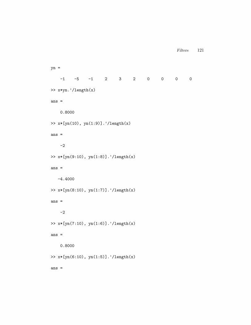
Filters 121
yn =
-1 -5 -1 2 3 2 0 0 0 0
>> x*yn.'/length(x)
ans =
0.8000
>> x*[yn(10), yn(1:9)].'/length(x)
ans =
-2
>> x*[yn(9:10), yn(1:8)].'/length(x)
ans =
-4.4000
>> x*[yn(8:10), yn(1:7)].'/length(x)
ans =
-2
>> x*[yn(7:10), yn(1:6)].'/length(x)
ans =
0.8000
>> x*[yn(6:10), yn(1:5)].'/length(x)
ans =

122 DSP Using MATLAB and Wavelets
1.9000
>> x*[yn(5:10), yn(1:4)].'/length(x)
ans =
1.3000
>> x*[yn(4:10), yn(1:3)].'/length(x)
ans =
0.4000
>> x*[yn(3:10), yn(1:2)].'/length(x)
ans =
1.3000
>> x*[yn(2:10), yn(1)].'/length(x)
ans =
1.9000
Technically, the value returned above is not the correlation, but the cross-covariance. One problem is that the shortcut used above only works when thesignal has an average of 0. Another problem with this value is that it does not tellus if the two signals are an exact match. That is, in the first example above, thecross-covariance between x and y was found to be 4.4, but if we were to comparesignal x with some other signal, could the cross-covariance be higher? Actually, theanswer is yes! The following two commands show why this is the case. Taking thesignal y and multiplying each value by 10, then finding the cross-covariance, leadsto an answer 10 times the original.
>> clear all
>> x = [ 0 0 1 5 1 -2 -3 -2 0 0 ];
>> y = [ 1 5 1 -2 -3 -2 0 0 0 0 ];

Filters 123
>> y10 = y*10
y10 =
10 50 10 -20 -30 -20 0 0 0 0
>> x*[y10(9:10), y10(1:8)].'/length(x)
ans =
44
To fix this, we find the cross-correlation, which uses two more pieces of infor-mation: the autocovariance for each signal. In the code, these are variables sxxand syy. The variable sxy is very similar to the above examples, except that noassumption is made about the signal averages.
The code below finds the cross-correlation between two signals.
%
% correlate.m - How much are 2 signals alike?
%
% Usage: [rho] = correlate(k, x, y);
% inputs: k = shift (integer between 0 and length(y)-1)
% x, y = the signals to correlate
% output: rho = the correlation coefficient -1..0..1
%
% Note: This function assumes length(x) = length(y).
%
function [rho] = correlate(k, x, orig_y)
% Shift y by k units
y = [orig_y(k+1:length(orig_y)), orig_y(1:k)];
N = length(x);
sxx = x*x.' - sum(x)*sum(x)/N;
syy = y*y.' - sum(y)*sum(y)/N;
sxy = x*y.' - sum(x)*sum(y)/N;

124 DSP Using MATLAB and Wavelets
rho = sxy / sqrt(sxx*syy);
When run, we see that the output rho (ρ), the cross-correlation, is a much bettervalue to use since it gives us an indication (up to 1) of how well the two signals match.
>> clear all
>> x = [ 0 0 1 5 1 -2 -3 -2 0 0 ];
>> y = [ 1 5 1 -2 -3 -2 0 0 0 0 ];
>> yn = -y;
>> y10 = y*10;
>> rho = correlate(8, x, y)
rho =
1
>> rho = correlate(8, x, y10)
rho =
1
>> rho = correlate(8, x, yn)
rho =
-1
The last example shows that a negative correlation exists between x and yn (thenegated version of y). The cross-correlation function takes care of the fact that thesignals may be scaled versions of each other. That is, we found that x and y10 abovewere a match, even though y10’s values were 10 times that of x’s.
Let us look at another example. What if we try to correlate x to a signal thatis not like it? We will call the second signal noise.
>> clear all
>> x = [ 0 0 1 5 1 -2 -3 -2 0 0 ];

Filters 125
>> noise = [ 0 -1 0 1 0 -1 1 0 1 -1];
>> for i=0:length(x)
my_rho(i+1) = correlate(i, x, noise);
end
>> my_rho
my_rho =
Columns 1 through 6
0.2462 -0.2462 -0.3077 0.3077 0.3693 0.4308
Columns 7 through 11
-0.2462 -0.3077 -0.3077 0.0615 0.2462
>> min_rho=min(my_rho); max_rho=max(my_rho);
>> if (abs(min_rho) > abs(max_rho))
min_rho
else
max_rho
end
max_rho =
0.4308
The array my rho stores all correlation coefficients for these two signals. To seehow well x and noise match up, we need to examine both the minimum as well asthe maximum values. With cross-correlation, we are able to say that two signalsmatch, or that they do not match well.
Example:The following example comes out of an image processing project. In Figure 3.30, wesee two rectangles. Our goal is to automatically match these two objects, somethingpeople can do easily, but is a difficult pattern-matching process for a computer.
The rectangles are similar, though one is smaller than the other, as well as being

126 DSP Using MATLAB and Wavelets
Figure 3.30: Two rectangles of different size (scale) and rotation.
rotated (i.e., one is longer than it is wide, the other is wider than it is long). Tohave the computer determine that they are a match, we will trace the boundariesof these objects, and calculate the center point. From this point, we will measurethe distance to each point that makes up the boundary, from the upper-left cornersclockwise around the object. When we finish, we have a one-dimensional view ofthese objects, as seen in Figure 3.31. The solid line represents the object on the leftin Figure 3.30, while the dotted points represent the object on the right.
Notice that the two have the same length. This is necessary for correlation, sothe smaller of the two was “stretched” to make it longer. The original signals ared1 and d2, and the code below shows a simple way to stretch the shorter signal d2to be the same length as d1. The first line creates an array of points at fractionalincrements. The second line makes a new data signal called d3 that is a copy of d2,with redundant points. Better ways to interpolate a signal exist (see the spline
command), but this method suffices for this example.
pts = 1:length(d2)/length(d1):length(d2)+1;
d3 = d2(round(pts(1:length(d1))));
Once we have two signals to compare that are the same length, we can use thecorrelation function, and take the largest value as an indication of how well theobjects match.
>> for k=1:length(d1)
rhos(k) = correlate(k, d1, d3);
end
>> disp(sprintf('max correlation coeff: %5.4f', max(rhos)));
max correlation coeff: 0.9994
Our code gives us a 0.9994 correlation coefficient, indicating a very good matchbetween the two objects, as expected.

Filters 127
0 50 100 150 200 250 300 350 400 45025
30
35
40
45
50
55
60
65
70
75Two rectangles (normalized) as 1D lengths from center. left:line, right:points
Figure 3.31: Two rectangles represented as the distance from their centers to theiredges.

128 DSP Using MATLAB and Wavelets
Example:To show that the previous example was not just a coincidence, we will repeat theabove experiment with a rectangle and a triangle, Figure 3.32.
Figure 3.32: A rectangle and a triangle.
This time, we see that the resulting one-dimensional signals are different, as wemight expect (Figure 3.33). With the rectangle, we see the 1D signal gradually getsmaller, then get larger again until it reaches the same height. Next, it gets a bitsmaller, then back to its original height. This pattern repeats. From the center, thecorners are going to be the furthest points away, and we see this as the top height.As we trace the boundary of the rectangle, the distance to the center gets a littlesmaller, then larger until we reach the next corner. As we trace the next side, thedistance gets smaller and then back to the original distance at the corner. Since thesecond side is not as long as the first, the gradual dip in height is not as prominent.With the triangle, the corners are not equidistant from the center (due to the useof a simple averaging function to find the center), thus we see three peaks in thedotted one-dimensional object representation, but two of them are not as far awayfrom the center as the third one. We started from the upper-right corner, thoughthe starting position does not matter since the correlation calculations consider theshift of the signal.
max correlation coeff: 0.6272
When we calculate the correlation coefficients, we find the maximum as only0.6272. We can conclude that that objects do share some similarity, but they arefar from a match.
3.9 Summary
Finite Impulse Response (FIR) filters are presented in this chapter, including theirstructure and behavior. Three important properties that FIR filters possess are

Filters 129
0 50 100 150 200 250 300 350 400 45010
20
30
40
50
60
70
80Two objects (normalized) as 1D lengths from center. left:line, right:points
Figure 3.33: A rectangle and triangle represented as the distance from their centersto their edges.

130 DSP Using MATLAB and Wavelets
causality, linearity, and time-invariance. Infinite Impulse Response (IIR) filters arealso a topic of this chapter. Correlation is covered here as well, which is one appli-cation of an FIR filter.
3.10 Review Questions
1. What does FIR stand for? What does it mean?
2. What does causal mean?
3. What does linear mean?
4. What does time-invariant mean?
5. Write MATLAB code to compute output (y[n]) for convolution, given any FIRfilter coefficients (b[k]) and input (x[n]).
6. Filter input x = [5, 1, 8, 0, 2, 4, 6, 7] with a 2-tap FIR filter of coefficients 1,−1 by hand (do not use a computer).
7. What word describes the operation below? of x[n] and b[n] producesy[n].
y[n] =K∑
k=0
b[k]x[n− k]
8. Make up a test signal of at least 10 values, and filter it with the followingcoefficients. Use MATLAB for this question.
a. b[k] = .4, .4b. b[k] = .2, .2, .2, .2c. b[k] = .1, .1, .1, .1, .1, .1, .1, .1
What do you observe? Which set of filter values do the best job of “smoothingout” the signal?
9. What do we call h[n]? Why is it significant?
10. What does MAC stand for? What does it mean?
11. For system1 and system2 below, are the systems linear? Are they time-invariant? Are they causal? Explain. Let x[n] be the input and y[n] be the out-put, where system1 is y1[n] = x[n]−x[n−1], and system2 is y2[n] = 3x[n]+1.

Filters 131
12. What is the difference between an FIR filter and an IIR filter? Draw one ofeach.
13. Suppose we have a system where y[n] = 2x[n] + x[n− 1].
a. Is this system causal?b. Is this system linear?c. Is this system time-invariant?
14. For the input signal x[n] = [6, 1, 3, 5, 1, 4], and a filter h[k] = [−1, 3,−1], findy[n], where y[n] = h[k] ∗ x[n]. Use the algorithm given in section 3.2.


Chapter 4
Sinusoids
Most analog signals are either sinusoids, or a combination of sinusoids (or can beapproximated as a combination of sinusoids). This makes combinations of sinusoidsespecially interesting. It is easy to add sinusoids together; pressing keys on a pianoor strumming a guitar adds several sinusoids together (though they do decay, unlikethe sinusoids we usually study). In this chapter, we will investigate sinusoids andsee how they can be added together to model signals. The goal is to gain a betterunderstanding of sinusoids and get ready for the Fourier transform.
4.1 Review of Geometry and Trigonometry
Greek letters are nothing to be afraid of. Mathematics uses variables, much like wedo in computer programming. These variables are one letter, which allows things tobe described concisely. Greek letters are often used simply because we tend to runout of our alphabetic letters. Also, there are letters that are good to avoid, like l,and o, since they look too much like the numbers 1 and 0.
Consider a right triangle (see Figure 4.1). We know, thanks to Pythagoras (orat least his school [15]) that a2 +b2 = c2, so if we happen to know only two sides, wecan calculate the third1. Also, with this information, we can figure out the anglesθ1 and θ2. Since it is a right triangle, the third angle is 90 degrees by definition.
The cosine function gives us the ratio of the length of the adjacent side (a) tothe length of the hypotenuse (c). In other words,
cos(θ1) =a
c.
1According to [16] the Babylonians knew this, but the Greeks were first to prove it.
133

134 DSP Using MATLAB and Wavelets
θ2
θ1
a
bc
Figure 4.1: A right triangle.
The sine function gives us the ratio of the length of the opposite side (b) to thelength of the hypotenuse (c). In other words,
sin(θ1) =b
c.
The cos−1 and sin−1 functions (also called arccos and arcsin) give us the angleθ1 from the ratio of the sides.
4.2 The Number π
It is impossible to talk about sine and cosine functions without talking about theconstant π, the ratio of a circle’s diameter to its circumference (see Figure 4.2). Youprobably remember the equation:
circumference = 2πr, where r is the circle’s radius.
+r−r
2 rπ
Lengtharound is
Figure 4.2: An example circle.

Sinusoids 135
Pi (π) is an irrational number. No matter how many digits you calculate it outto be, someone else could go a digit further. To date, no repeating pattern has beenfound, so unlike rational numbers, you cannot represent π in a compact form. Forexample, with a rational number such as 1
3 , you could write it as 0.33 to indicatethat it repeats forever when represented as a decimal number, or at least it can berepresented as one number (1) divided by another (3).
Ancient peoples had various approximations for π. The Egyptians used 256/81for π, while the Babylonians calculated with 3 1
8 [17]. We will use the approximationof 3.1415927 for π.
We will specify sinusoid components with the format
a× cos(2πft+ φ)
where a is the amplitude, f is the frequency, and φ is the phase angle. The variablet represents time. Sine could be used in place of cosine, if we add π/2 to the phaseangle, since cos(θ) = sin(θ + π/2).
Amplitude (a), phase shift (φ) (also called the phase angle), and frequency com-pletely specify a sinusoid. Amplitude describes a quantity without assigning it units.Magnitude is also a unitless description of a quantity, with one difference: ampli-tude can be positive or negative, while magnitude is always positive [11]. |x(t)|refers to magnitude, and as you may expect, the abs function in MATLAB returnsthe magnitude. Many people in DSP use magnitude and amplitude interchangeably,for good reason. Viewing a sinusoid component as a phasor, where we draw it inits initial position without concern about rotation with time, we would draw thephasor along the positive x-axis, then rotate it counterclockwise according to thephase angle. A negative length means we would draw the phasor along the negativex-axis, then rotate (again counterclockwise) according to the angle. However, thisis exactly the same as drawing the length along the positive x-axis, and rotating itan additional 180 degrees. In other words, −a× cos(2πft+ φ) is exactly the sameas a × cos(2πft + φ + π). This is why we typically use a positive value for theamplitude. The main exception is for the DC component, where frequency equalszero. The phase angle also is assumed to be zero, and thus the amplitude is theonly value left to determine the sign of the DC component.
We use f to represent the cyclic frequency, also called simply frequency, thoughsometimes the radian frequency (ω) is used for convenience. It relates to f with theequation ω = 2πf . The units of f are in Hz, cycles per second, named for Hein-rich Hertz (1857–1894), a German physicist whose experiments confirmed Maxwell’selectromagnetic wave theories [18]. Since the unit Hz comes from a person’s name,the first letter should always be capitalized.

136 DSP Using MATLAB and Wavelets
4.3 Unit Circles
A unit circle is of particular interest. For a unit circle, the radius r equals 1.Therefore, the circumference, or length of the circle if it were cut and unrolled, is2π. As a result, we can talk about an angle in terms of the length of the arc betweentwo line segments joined at a point. We call this angle radians (rad for short). InFigure 4.3, angle θ is only a fraction of the circle’s circumference, therefore, it is afraction of 2π. Figure 4.4 shows the arc lengths on a unit circle for several commonangles.
θ
Figure 4.3: An angle specified in radians.
No doubt you are also familiar with an angle measured in degrees. When dealingwith sinusoidal functions (such as sine, cosine, etc. ), it is important to know whetherthe function expects the argument to be in degrees or radians. On a scientificcalculator, you are likely to have a button labeled DRG, to allow you to specifydegrees or radians, though the default is probably degrees. For MATLAB, C/C++and Java, the arguments to the sin() and cos() functions are assumed to be radians.
To convert between degrees and radians, we recall that one complete rotationaround the unit circle’s edge is 2π radians, or 360. To convert from degrees toradians, therefore, we multiply by 2π/360. To convert from radians to degrees, wemultiply by 360/(2π). For example, suppose the angle shown in Figure 4.3 is 30,
(30)(2π/360) = 60π/360
= π/6 radians.
Converting π/6 back to degrees can be done in a similar fashion:

Sinusoids 137
π/2
π
3π/2
2π
Figure 4.4: An angle specified in radians.

138 DSP Using MATLAB and Wavelets
(π/6)(360/(2π)) = 360π/(12π)
= 360/12
= 30.
Quiz: What is larger, cos(0) or cos(1, 000, 000)? At first glance, one unfamiliarwith the cosine function might assume that the latter is larger, simply because theargument is larger. But since sinusoids repeat, there is no reason for this to be thecase. In fact, one might remember that cos(0) is 1, and that cos(any number) alwaysgenerates a value between +1 and −1. Therefore, cos(0) is going to be greater thanor equal to cos(any number). In fact, cos(1, 000, 000) ≈ 0.9368, correct? If not, it islikely due to your calculator being in degrees mode! Since it was not specified thatthe angle is in degrees, one should assume that it is in radians.
Another thing to consider when dealing with sinusoid functions is that they arerepetitive. The angle specified by 0 radians is the same as that specified by 2πradians. Thus, you can always add or subtract 2π to/from an angle. In fact, youcan add or subtract any integer multiple of 2π to or from an angle. Sometimes thismakes things easier.
4.4 Principal Value of the Phase Shift
A sinusoid stretches out infinitely in both directions. If we want to view it in termsof a time axis, we can use the positive peaks of the sinusoid to relate to our timeaxis. Figure 4.5 shows an example sinusoid, cos(2π60t), with a frequency of 60 Hz.Therefore, the period of time before this sinusoid repeats is 1
60 , or 0.0167 seconds.Vertical lines show where one repetition starts and ends, at t = −0.0167/2 and t =+0.0167/2. This corresponds to arguments of −π and +π for the cos function, thatis, let t = ( 1
60 )(−12 ) to make cos(2π60t) equal cos(2π60(1/60)(−1/2)) = cos(−π).
But WHICH peak do we normally use? In Figure 4.5 it is very easy, but asinusoid function often has a nonzero phase angle. Since it repeats every 2π, wecould pick any peak that we want to classify the signal. This means that there willalways be a positive peak between -π and +π, in other words, −π < φ ≤ +π whereφ is the phase shift [6].
So why not use the positive peak closest to zero? This makes a lot of sense, andwe give this peak a special name: we say it is the principal value of the phase shift.To find this peak, we can always add/subtract 2π from the phase shift, until it is inthe range we desire.

Sinusoids 139
−0.05 −0.04 −0.03 −0.02 −0.01 0 0.01 0.02 0.03 0.04 0.05−1
−0.5
0
0.5
1
time
ampl
itude
Figure 4.5: A 60 Hz sinusoid.
4.5 Amplitudes
Usually, amplitude values are positive, and for good reason. Consider two sinusoidsof the same frequency, x1 = a× cos(2πft+ φ1) and x2 = −a× cos(2πft+ φ2). Weknow that the minimum and maximum values for the cosine function are -1 and +1.Therefore, x1 varies between +a and −a, and x2 varies between −a and +a. Giventhat the two sinusoids have the same frequency, they must look a lot alike. In fact,the only difference between them is their phase angles, a difference of π. That is,φ2 = φ1 +π. This makes a lot of sense considering the conversion of a complex valueof x+ jy to polar form r∠θ: the equation (
√
x2 + y2) leads to a positive value forr. A vector with a negative length would be the same as a vector with a positivelength, rotated a half-revolution, as demonstrated in Figure 4.6.
real axis
imaginary axis
j
θreal axis
imaginary axis
j
θ
−aθ
a
Figure 4.6: A vector of −a at angle θ = a at angle (θ + π).
Signals are often represented as a sum of sinusoids. When these sinusoids arerelated, we call the signal a harmonic.

140 DSP Using MATLAB and Wavelets
4.6 Harmonic Signals
Real-world signals can be decomposed into a set of sinusoids added together. Aharmonic signal is composed of several sinusoids added together, each with an integermultiple of some base frequency, called the fundamental frequency. For example, thefollowing signal is a harmonic:
x(t) = 0.4 cos(2π15t + π/5) + 0.7 cos(2π30t) + cos(2π45t − π/4).
Signal x(t) is of the form
a1 × cos(2π(1)f0t+ φ1) + a2 × cos(2π(2)f0t+ φ2) + a3 × cos(2π(3)f0t+ φ3)
where, for x(t), a1 = 0.4, a2 = 0.7, a3 = 1, φ1 = π/5, φ2 = 0, φ3 = −π/4, andf0 = 15 Hz. Any signal of this form is a harmonic.
If an amplitude value is 0, then the corresponding sinusoid will not contributeto the function. In other words, 0 × cos(anything) evaluates to 0. If we have afunction like
x2(t) = 0.1 cos(2π100t − π/6) + 1.3 cos(2π300t + π) + 0.5 cos(2π400t + 2π/3)
then x2(t) is a harmonic with a1 = 0.1, a2 = 0, a3 = 1.3, a4 = 0.5, φ1 = −π/6,φ2 = 0, φ3 = π, φ4 = 2π/3, and f0 = 100 Hz.
The following MATLAB code is a function to plot harmonic signals.
%
% Given magnitudes, phases, and the fundamental frequency,
% plot a harmonic signal.
%
% Usage: plotharmonic(freq, mag, phase)
%
% where freq = the fundamental frequency (a single value),
% mag = the amplitudes (a list),
% phase = the phases (a list).
%
function plotharmonic(freq, mag, phase)
num_points = 200; % Number of points per repetition
% Check parameters
if (size(mag) ~= size(phase))

Sinusoids 141
sprintf('Error - magnitude and phase must be same length')
end
% We want this for 2 repetitions, and num_points per rep.
step = 2/(freq*num_points);
t = 0:step:2*(1/freq);
clear x;
x = 0;
for i=1:length(mag)
x = x + mag(i)*cos(2*pi*i*freq*t + phase(i));
end
my_title = sprintf('Harmonic signal: %d sinusoids',length(mag));
plot(t,x);
title(my_title);
xlabel('time (sec)');
ylabel('Amplitude');
For example, the following commands plot x2(t) from above. It is assumed thatthe code from above is saved with “plotharmonic.m” as the filename.
Mag = [ 0.1 0 1.3 0.5];
Phase = [ -pi/6 0 pi 2*pi/3];
plotharmonic(100, Mag, Phase); % Fundamental freq. is 100 Hz
The resulting plot can be seen in Figure 4.7.One additional piece of information is if there is a vertical shift of the signal.
That is, what if the graph shown in Figure 4.7 was not centered around the x-axis?This can be accomplished by adding a constant to the signal. For example, if we add100 units to the signal, it would look the same, but it would be centered around theline y = 100. This piece of information can be added to the above harmonic signalformat, simply by including the term a0 cos(2π(0)f0t+ φ0). Starting the multiplesof f0 at zero means that the first component is simply a constant. There is noneed to specify a φ0 term, since cos(φ0) would just be a constant, and a0 alreadyspecifies this. Therefore, we will assume φ0 is zero. This term is often called theDC component, for Direct Current.
Example:For the signals below, say which ones are harmonic and which are not. If they

142 DSP Using MATLAB and Wavelets
0 0.002 0.004 0.006 0.008 0.01 0.012 0.014 0.016 0.018 0.02−2
−1.5
−1
−0.5
0
0.5
1
1.5
2Harmonic signal with 4 sinusoids
Time (sec)
Am
plitu
de
Figure 4.7: A harmonic signal.

Sinusoids 143
are harmonic, say what the fundamental frequency is.
x1(t) = 2 cos(2π7t) + 3 cos(2π35t)x2(t) = 2 cos(2π2t) + 3 cos(2πt)x3(t) = 2 cos(2π7t + π) + 3 cos(2πt− π/4)
Answer:To be harmonically related, each sinusoid must have a frequency that is an
integer multiple of some fundamental frequency. That is, they should be in thefollowing form. Remember that k is an integer.
x(t) =
N∑
k=1
ak cos(2πkf0t+ φk)
So we put the above signals in this form, and see if the k values are integers,which they must be for the sinusoids to be harmonically related. Looking at thearguments of the cosine function for x1, let k1 and k2 be values of k.
2π7t = 2πk1f0t+ φk, Let φk = 0f0 = 7/k1
2π35t = 2πk2f0t+ φk, Let φk = 0f0 = 35/k2
Substituting in f0, we get
35/k2 = 7/k1
k1/k2 = 7/35k1/k2 = 1/5
So if k1 = 1, then k2 = 5
f0 = 35/k2 = 35/5 = 7 Hz.Therefore, x1(t) has integer k values, and is harmonic. x3(t) is, too. x2(t)
does not have integer k values (due to the frequency of π) and is, therefore, notharmonic. The third signal, x3, is a bit tricky because the frequency componentsare not lined up as we may expect.f0 = 1 Hz, a0 = 1, ak = 3, 0, 0, 0, 0, 0, 2, andφk = −π/4, 0, 0, 0, 0, 0, π.

144 DSP Using MATLAB and Wavelets
We could consider harmonic a signal with a DC component, too. Without lossof generality, we can have index k start at 0, implying that we have a frequencycomponent of 0 ∗ f0, or 0 Hz. Since designating a value for the phase angle wouldonly result in the amplitude a0 being multiplied by a constant, we should set thephase angle to 0. Thus, a0 completely specifies the DC component.
Representing a signal that has discontinuities, such as a square wave, with a sumof harmonically related sinusoids is difficult. Many terms are needed [19]. CalledGibbs’ phenomenon, we cannot perfectly represent a discontinuous signal as a sumof sinusoids, but our approximation will have overshoot, undershoot, and ripples.
Fourier analysis works best with a periodic signal. We implicitly expect that thefirst and last sample are linked, that if we were to take one more reading of thesignal, that this reading would be the same as the very first sample, or at least avalue that we have seen before. Whether or not this N + 1 value matches value 0depends upon how many samples we have taken. Also, we assume that a sufficientnumber of samples has been recorded, given by the sampling period. If the signaltruly is periodic, and we have a good sampling rate, and we take exactly one period’sworth of samples, then the sample at N + 1 would be equal to sample 0.
Sometimes we do not have a periodic signal. In this case, we may have a dis-continuity between the last sample and the first. For example, consider the signalbelow, Figure 4.8:
Figure 4.8: A short signal.
If we treat this signal as being periodic, then we expect that it repeats forever,and that we can copy and paste this signal to itself, such as in Figure 4.9.
Here we see that there is a discontinuity in the middle, and this is difficult for aFourier series to handle (remember Gibb’s phenomenon). Thus, we should considerthe Fourier analysis to give us an approximation of the original signal. We wouldexpect that the approximation is not as good around a discontinuity as it is for therest of the signal. We call this difficulty edge effects.
Even with edge effects, Fourier analysis will return a good approximation to the

Sinusoids 145
Figure 4.9: The short signal, repeated.
original signal. In fact, any nonrandom signal can be approximated with Fourieranalysis. If we take a random signal and find the Fourier series of it, we will findthat it approximates the signal for the values that we have seen. However, we maybe tempted to use this to predict future values of the signal. If it is truly random,though, any matching between the signal and a prediction would be coincidence.
4.7 Representing a Digital Signal as a Sum of
Sinusoids
A digital signal can be represented as a sum of sinusoids. The following three figuresshow how this works. We can take a digital signal and find the Fourier transform ofit (the Fourier transform is covered a bit later in this book). The important thingto understand is that the Fourier transform gives us a frequency-domain version ofthe signal: a list of amplitudes and phase angles corresponding to a harmonicallyrelated set of sinusoids.
We explore the fundamental frequency of these sinusoids later; for the presentdiscussion, we will ignore it. The timing of these simulated samples determines thereal fundamental frequency, so we will just stick to sample numbers instead of timefor the x-axis of the plots.
Refer to Figure 4.10. Here we see the original signal, a list of discrete samplepoints. Under it, we have a graph of a signal made by adding several sinusoids (8,to be precise). Notice how this composite signal passes through the same points asthe original digital signal. If we were to read values from this composite signal withthe same timing as the sampling of the digital signal, we would have the same data.
In Figure 4.10, we see that the sum of sinusoids representation is continuous.But we should be careful not to conclude that the underlying analog signal, which weare trying to represent as a set of discrete points, actually looks like the composite

146 DSP Using MATLAB and Wavelets
0 1 2 3 4 5 6 72
3
4
5
6
7
8original
0 1 2 3 4 5 6 72
3
4
5
6
7
8sum of sinusoids
Figure 4.10: A digital signal (top) and its sum of sinusoids representation (bot-tom).

Sinusoids 147
signal. We may not know what it looks like, and the hill we have between sample 2and sample 3 (as well as between sample 3 and sample 4) could mislead us.
The next two graphs, Figures 4.11 and 4.12, show the sinusoids that we addedtogether to get the composite one. Yes, the first one shown is a sinusoid of zerofrequency! The asterisks show the values that would be found if the sinusoids weresampled with the same timing as the original signal. Notice how the number ofsinusoids (8) returned from the Fourier transform matches the number of originalpoints (8).
0 1 2 3 4 5 6 72
4
6
0 1 2 3 4 5 6 7−1
0
1
0 1 2 3 4 5 6 7−1
0
1
0 1 2 3 4 5 6 7−1
0
1
ampl
itude
sample
Figure 4.11: The first four sinusoids in the composite signal.
As an exercise, let’s approximate the value of the second-to-last sample. InFigure 4.11, we see that sample #6 of each sinusoid has the following approximatevalues: 4.9, 0.3, -0.1, and 0.7. Turning our attention to Figure 4.12, we see thisnext-to-last sample’s values are roughly: 0.4, 0.7, -0.1, and 0.3. If we add these uptogether, we get 7.1. Looking back at the original Figure 4.10, we see that the valuefor sample #6 is right around 7. In fact, the only reason we did not get exactlythe same number as in the first figure was due to the error induced by judging the

148 DSP Using MATLAB and Wavelets
graphs by eye.
0 1 2 3 4 5 6 7−0.5
0
0.5
0 1 2 3 4 5 6 7−1
0
1
0 1 2 3 4 5 6 7−1
0
1
0 1 2 3 4 5 6 7−1
0
1
ampl
itude
sample
Figure 4.12: The last four sinusoids in the composite signal.
In a similar exercise, we can note the maximum values for each of the sinusoidsin Figures 4.11 and 4.12. These are: 4.88, 0.86, 0.76, 0.81, 0.38, 0.81, 0.76, and0.86. They correspond to the amplitudes of each of the sinusoids, the ak valuesthat we would need for a harmonic representation. The other pieces of information(besides the fundamental frequency) would be the phase angles. These are a bitmore difficult to read off of a graph, but we can make approximations for them.Remembering that cos(0) = 1, we notice that the value returned from the cosinefunction decreases as the angle gets larger, until it reaches −1 at π, then it increasesuntil it gets to 1 again at 2π. We can use this observation to get a rough idea aboutthe phases. Looking at the second graph of Figure 4.11, we see that the sinusoidhas its maximum point right at sample 0. The maximum point would correspondto the amplitude, or more exactly a1 × cos(2π1f0t+ φ1) when the argument to thecosine function is 0, as it would be at time 0. So we would have 2π1f00 + φ1 = 0,or simply φ1 = 0. Now, to find the next phase angle, φ2. At sample 0 (third
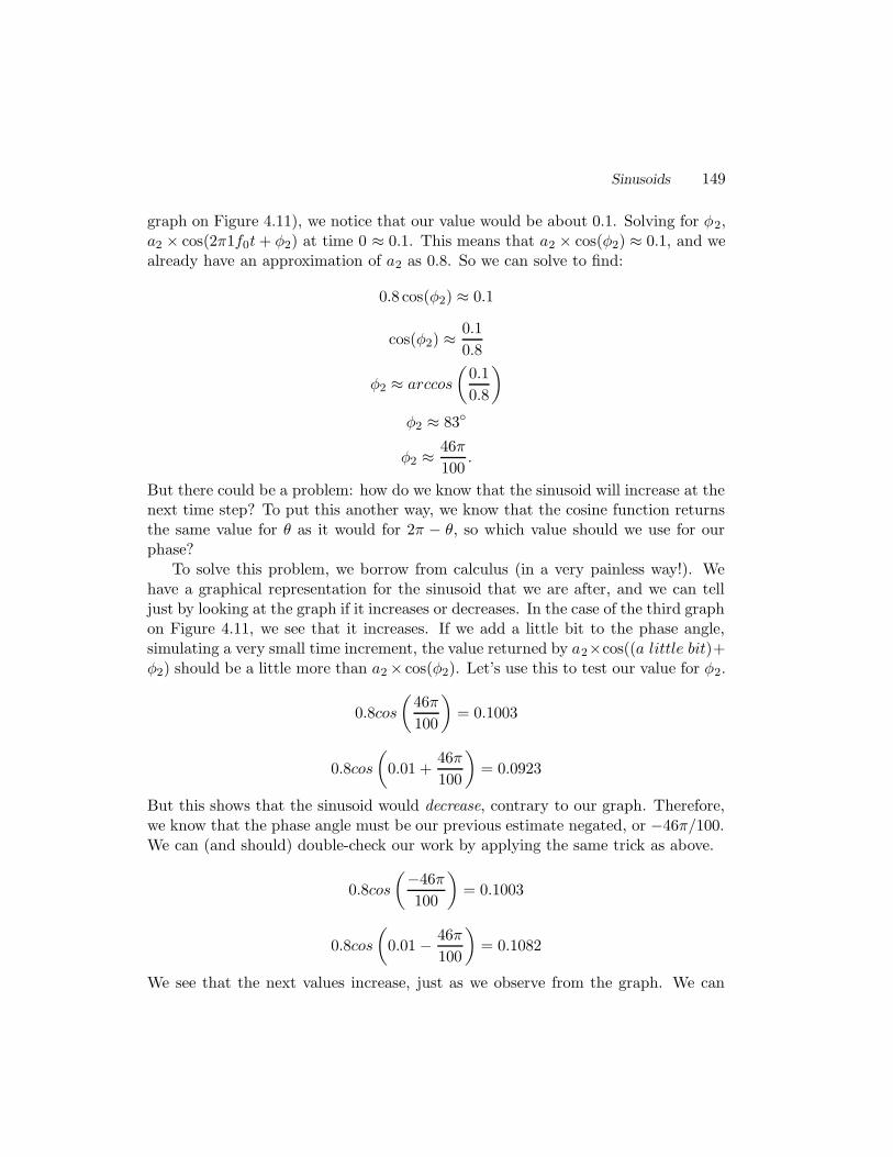
Sinusoids 149
graph on Figure 4.11), we notice that our value would be about 0.1. Solving for φ2,a2 × cos(2π1f0t+ φ2) at time 0 ≈ 0.1. This means that a2 × cos(φ2) ≈ 0.1, and wealready have an approximation of a2 as 0.8. So we can solve to find:
0.8 cos(φ2) ≈ 0.1
cos(φ2) ≈0.1
0.8
φ2 ≈ arccos
(
0.1
0.8
)
φ2 ≈ 83
φ2 ≈ 46π
100.
But there could be a problem: how do we know that the sinusoid will increase at thenext time step? To put this another way, we know that the cosine function returnsthe same value for θ as it would for 2π − θ, so which value should we use for ourphase?
To solve this problem, we borrow from calculus (in a very painless way!). Wehave a graphical representation for the sinusoid that we are after, and we can telljust by looking at the graph if it increases or decreases. In the case of the third graphon Figure 4.11, we see that it increases. If we add a little bit to the phase angle,simulating a very small time increment, the value returned by a2×cos((a little bit)+φ2) should be a little more than a2 × cos(φ2). Let’s use this to test our value for φ2.
0.8cos
(
46π
100
)
= 0.1003
0.8cos
(
0.01 +46π
100
)
= 0.0923
But this shows that the sinusoid would decrease, contrary to our graph. Therefore,we know that the phase angle must be our previous estimate negated, or −46π/100.We can (and should) double-check our work by applying the same trick as above.
0.8cos
(−46π
100
)
= 0.1003
0.8cos
(
0.01 − 46π
100
)
= 0.1082
We see that the next values increase, just as we observe from the graph. We can

150 DSP Using MATLAB and Wavelets
continue in like fashion for the rest of the graphs.The program below demonstrates the sum-of-sinusoids concept. It does not
require any parameters, since it makes the “original” signal randomly. This programfinds the frequency-domain representation X of the random signal x, then uses thefrequency-domain information to get the original signal back again (as the arraymy sum of sins). We see that, when run, this program calculates the error betweenthe original signal and the reconstructed one, an error so small that it is due onlyto the precision used.
% sum_of_sins.m
% Show a random signal as a sum of sins
%
% Make our x signal
x = round(rand(1,8)*10);
Xsize = length(x);
% Get FFT of x
X = fft(x);
Xmag = abs(X);
Xphase = angle(X);
% Show the freq-domain info as sum of sinusoids
% Find the IFFT (the hard way) part 1
n=0:Xsize-1; %m=0:Xsize-1;
% Do the sinusoids as discrete points only
s0 = Xmag(1)*cos(2*pi*0*n/Xsize + Xphase(1))/Xsize;
s1 = Xmag(2)*cos(2*pi*1*n/Xsize + Xphase(2))/Xsize;
s2 = Xmag(3)*cos(2*pi*2*n/Xsize + Xphase(3))/Xsize;
s3 = Xmag(4)*cos(2*pi*3*n/Xsize + Xphase(4))/Xsize;
s4 = Xmag(5)*cos(2*pi*4*n/Xsize + Xphase(5))/Xsize;
s5 = Xmag(6)*cos(2*pi*5*n/Xsize + Xphase(6))/Xsize;
s6 = Xmag(7)*cos(2*pi*6*n/Xsize + Xphase(7))/Xsize;
s7 = Xmag(8)*cos(2*pi*7*n/Xsize + Xphase(8))/Xsize;
% Redo the sinusoids as smooth curves
t = 0:0.05:Xsize-1;
smooth0 = Xmag(1)*cos(2*pi*0*t/Xsize + Xphase(1))/Xsize;
smooth1 = Xmag(2)*cos(2*pi*1*t/Xsize + Xphase(2))/Xsize;
smooth2 = Xmag(3)*cos(2*pi*2*t/Xsize + Xphase(3))/Xsize;
smooth3 = Xmag(4)*cos(2*pi*3*t/Xsize + Xphase(4))/Xsize;

Sinusoids 151
smooth4 = Xmag(5)*cos(2*pi*4*t/Xsize + Xphase(5))/Xsize;
smooth5 = Xmag(6)*cos(2*pi*5*t/Xsize + Xphase(6))/Xsize;
smooth6 = Xmag(7)*cos(2*pi*6*t/Xsize + Xphase(7))/Xsize;
smooth7 = Xmag(8)*cos(2*pi*7*t/Xsize + Xphase(8))/Xsize;
% Find the IFFT (the hard way) part 2
my_sum_of_sins = (s0+s1+s2+s3+s4+s5+s6+s7);
smooth_sum = smooth0 + smooth1 + smooth2 + smooth3;
smooth_sum = smooth_sum + smooth4 + smooth5 + smooth6 + smooth7;
% Show both discrete points and smooth curves together
xaxis1 = (0:length(smooth0)-1)/20; % for 8 points
xaxis2 = (0:length(s0)-1);
figure(1);
subplot(4,1,1); plot(xaxis1, smooth0, 'g', xaxis2, s0, 'r*');
subplot(4,1,2); plot(xaxis1, smooth1, 'g', xaxis2, s1, 'r*');
subplot(4,1,3); plot(xaxis1, smooth2, 'g', xaxis2, s2, 'r*');
subplot(4,1,4); plot(xaxis1, smooth3, 'g', xaxis2, s3, 'r*');
ylabel('amplitude');
xlabel('sample');
figure(2);
subplot(4,1,1); plot(xaxis1, smooth4, 'g', xaxis2, s4, 'r*');
subplot(4,1,2); plot(xaxis1, smooth5, 'g', xaxis2, s5, 'r*');
subplot(4,1,3); plot(xaxis1, smooth6, 'g', xaxis2, s6, 'r*');
subplot(4,1,4); plot(xaxis1, smooth7, 'g', xaxis2, s7, 'r*');
ylabel('amplitude');
xlabel('sample');
% Show the original versus the reconstruction from freq-domain
figure(3);
subplot(2,1,1); plot(0:Xsize-1, x, 'bd');
title('original');
min_y = floor(min(smooth_sum));
max_y = ceil(max(smooth_sum));
axis([0, Xsize-1, min_y, max_y]); % Make the axes look nice
xaxis1 = (0:length(smooth_sum)-1)/20;
xaxis2 = (0:length(s0)-1);
subplot(2,1,2);

152 DSP Using MATLAB and Wavelets
plot(xaxis1, smooth_sum, 'b', xaxis2, my_sum_of_sins, 'rd');
title('sum of sinusoids');
Error = my_sum_of_sins - x
We assume that the signal contains only real information. In general, this isnot the case. However, since we started with a signal of all real values, we willend up with a signal of all real values, since we do not change the information, weonly transform it from the time-domain to the frequency-domain, then transformit back. The Fourier transform results in a complex signal, though the originalsignal was real. To reconcile this, we simply treat the original real signal as if itwere complex, but the imaginary part is zero. The signal returned from the inverse-transform must also have an imaginary part of zero for all values. The programperforms the inverse-transform in a sense, but it does not take the complex part intoconsideration, as it would have to do if the original signal were complex. In otherwords, the program treats each sinusoid as if it were Xmag[k] cos(2πkf0t+Xangle[k]),when in fact each sinusoid is (from Euler’s formula)Xmag [k] cos(2πkf0t+Xangle[k])+jXmag [k] sin(2πkf0t +Xangle[k]). We are able to get away with this simplificationsince we know in advance that the complex parts, j sin(), must cancel each otherout.
4.8 Spectrum
A spectrum is the name given to the frequency plot of a signal. The spectrum isa graph of the frequencies that make up a signal, with their amplitudes shown inrelation to each other. A separate graph shows the phases for each sinusoid.
Previously, in Figure 4.10, we saw that a digital signal can be represented bya sum of sinusoids. These sinusoids can then be graphed individually, as shown inFigures 4.11 and 4.12. Sometimes this sinusoid information provides insight into thesignal. For example, if the original signal is music, then the sinusoids tell us aboutthe instruments that are being played. If the original signal was of a person talking,with a high-pitched extraneous sound such as a train whistle, we might be able toremove the higher-frequency whistle.
Plotting the information given to us by the sinusoids results in a spectrum. Con-tinuing with the example from the last section, we see that one piece of informationwe are missing is the fundamental frequency. As stated before, we need to know howmuch time there is between samples before we can know the frequencies. But we willdo our best without this. We see that the sinusoids repeat an integral amount in eachgraph, from 0 repetitions (0 frequency) up to 7 repetitions. That is, the sinusoids re-peat with such a frequency that sample #8, if plotted, would be the same as sample

Sinusoids 153
#0. As the number of repetitions gets larger, so does the corresponding frequency.Suppose, for the sake of argument, that the original signal was sampled at a rate of125 milliseconds per sample, so we read each sample 125 milliseconds after the last.The second graph, on Figure 4.11, shows that the sinusoid repeats once every 1000milliseconds, or once per second (it takes another 125 milliseconds before it gets tosample #8, which is identical to sample #0). Thus, it has a frequency of 1 Hz.Similarly, we see that the next graph has a frequency of 2 Hz, then 3 Hz for the nextgraph, etc., up to 7 Hz for the last graph of Figure 4.12. For the remainder of thischapter, we assume that we have this fundamental frequency of 1 Hz. Recalling ouramplitudes 4.88, 0.86, 0.76, 0.81, 0.38, 0.81, 0.76, 0.86 from the previous section,and getting the corresponding phases in degrees 0, 22,−81,−56, 0, 56, 81,−22, wecan plot this information as follows, Figure 4.13. In the top part of the figure, wesee a frequency magnitude plot, since it shows the positive amplitudes versus thefrequencies. The bottom part of Figure 4.13 shows a frequency phase plot, since itshows the phase angles for each corresponding sinusoid frequency.
−22
(Hz)2 3 4 60 1 5 7
frequency(Hz)
2 3 4 60 1 5 7
0.760.86 0.81 0.760.81 0.86
0.38
4.88
amplitude
(degrees)phase
0
81
220
−81−56
56
frequency
Figure 4.13: Frequency magnitude spectrum and phase angles.
One should observe the pattern of the spectrum: for the frequency magnitudeplot, we see a mirror image centered around 4 Hz. On the phase plot, again thepattern centers around 4 Hz, but we have a flipped as well as mirrored image.
So far we have seen how to get the spectrum from the amplitudes and phasesreturned by the Fourier transform. To find the spectrum of an abstract signal, suchas a mathematical model, use the inverse Euler’s formula. Here we have only an

154 DSP Using MATLAB and Wavelets
introduction; this topic is covered extensively in Chapter 7, “The Number e.” Forexample, to find and plot the magnitude spectrum of x(t) = 2 +2 cos(2π(200)t), weput it in terms of cosine functions.
x(t) = 2 + 2 cos(2π200t)= 2 cos(0) + 2 cos(2π200t)
Next, use inverse Euler’s formula:
cos(φ) = (ejφ + e−jφ)/2.
Notice how this results in two frequency components: one at the frequency given,and one at the negative frequency. For the spectrum, this implies that the range offrequencies will be different from what we saw with the previous example. Actually,the information stays the same, only our spectral plot has different, but equivalent,frequency values. This is explained in Chapter 6, “The Fourier Transform.”
x(t) = 2(ej0 + e−j0)/2 + 2(ej2π(200)t + e−j2π(200)t)/2
= 2(1 + 1)/2 + (2/2)(ej2π(200)t + e−j2π(200)t)
= 2 + ej2π(200)t + e−j2π(200)t
This results in a magnitude of 2 at frequency 0 Hz, and a magnitude of 1 atfrequencies 200 Hz and -200 Hz. This is shown in the magnitude plot, Figure 4.14.
0 Hz
1
2
1
−200 200−300 −100 100 300
Figure 4.14: Spectrum plot: magnitude of x(t) = 2 + 2 cos(2π(200)t).
Example:For the signal x(t) below,
x(t) = 4 cos(2π100t + 3π/4) + 2 cos(2π200t) + 5 cos(2π300t − 3π/5)
draw the magnitude spectrum and the phase spectrum of this signal.

Sinusoids 155
Answer:
x(t) =4
2ej(2π100t+3π/4) +
4
2e−j(2π100t+3π/4)
+2
2ej(2π200t) +
2
2e−j(2π200t)
+5
2ej(2π300t−3π/5) +
5
2e−j(2π300t−3π/5)
x(t) = 2 ej2π100tej3π/4 + 2 e−j2π100te−j3π/4
+ ej2π200t + e−j2π200t
+ 2.5 ej2π300te−j3π/5 + 2.5 e−j2π300tej3π/5
Pulling the frequencies out 100,−100, 200,−200, 300,−300 , and marking thecorresponding magnitudes 2, 2, 1, 1, 2.5, 2.5, gives us the graph of Figure 4.15. Foreach frequency, we also note the phases, 3π/4,−3π/4, 0, 0,−3π/5, 3π/5. Thephase angles are shown in Figure 4.16.
0 Hz
2.5 2.5
−300 300100 200−100−200
22
1 1
Figure 4.15: Spectrum plot: magnitudes.
0 Hz−300 300100 200−100−200
0 0
−3π/5
3π/5
−3π/4
3π/4
Figure 4.16: Spectrum plot: phase angles.

156 DSP Using MATLAB and Wavelets
4.9 Summary
Real-world signals have sinusoid components, unless they are truly random, in whichcase they can still be approximated with a sum of sinusoids. Since all analog signalscan be represented (or at least approximated) with a sum of sinusoids, we can viewa signal in terms of the frequencies that comprise it. Given a sum-of-sinusoidsequation for a signal, we use the inverse Euler’s formula to convert to a sum ofcomplex exponentials, such as (a1/2)e
j2πf1tejφ1 + (a1/2)ej2π(−f1)tej(−φ1). From this
form, we can make a plot of the amplitudes (a1/2, a1/2) versus the frequencies (f1,−f1), as well as a plot of the phase angles versus the frequencies. Together, we callthis information the spectrum, a view of the signal in the frequency-domain.
We will see how to get the frequency-domain information from a signal of onlytime-domain points using the Fourier transform, in Chapter 6.
4.10 Review Questions
1. What are the minimum and maximum values for x(t)?
x(t) = 3 cos(2π100t + π/6)
2. Given sin(θ) = cos(θ−π/2), if x(t) = 3 sin(2π100t+π/6), what is this functionin terms of cos?
3. The analog signal, x(t), is:
x(t) = 3 cos(2π2000t + π/4) + 2 cos(2π5000t) + cos(2π11000t − π/7)
a. plot each frequency component (in the time-domain) separatelyb. graph this function (in the time-domain)c. represent x(t) in terms of a fundamental frequency, amplitudes and phases.
4. The analog signal, x(t), is:
x(t) = 3 cos(2π3000t) + cos(2π1000t + π/3) + 4 cos(2π5000t − π/3)
Represent x(t) in terms of a fundamental frequency, amplitudes and phases.
5. What is the difference between amplitude and magnitude? What does |x(t)|mean?
6. DC component specifies the “shift of the signal” . (f = 0)

Sinusoids 157
Phase-shift specifies shift of signal . (φ)
7. What is another name for a plot of the frequency information of a signal?
8. Which signal, a square wave or a triangular wave, is easier to approximatewith a series of harmonically related sinusoids? Why?
9. Why are amplitudes always positive?
10. Since x(t) below is in the form a0 +∑N
k=1 ak cos(2π(k)f0t+ φk), what are thevalues for N , ak, φk, and f0 ? What special name do we give this signal x(t)?
x(t) = 4 + 3 cos(2π(1)20t + π/2) + 7 cos(2π(2)20t − 2π/3)


Chapter 5
Sampling
We live in an analog world, in that the signals that interest us are typicallycontinuous. Our computers are digital devices, meaning that they can store onlyfinite, discrete data, limited in both precision and magnitude. Thus, we need toapproximate signals before we can store and manipulate them. How do we bridgethe gap between the real world and the synthetic one of our computers? This chapteraddresses this central question.
Sampling is the process of getting a digital signal from an analog one. Whenwe sample a signal, we record, every so often, a value. Sampling can lead to manydata values. For example, a 3-minute song, sampled at 16 bits at 44,100 Hz (for twochannels), produces:
(3 minutes) ×(
16 bitssample
)
×(
44100 samplessecond
)
× 2.
Changing the units to make them uniform makes this:
(
3 minutes 60 seconds1 minute
)
×(
16 bitssample
1 byte8 bits
)
×(
44100 samplessecond
)
× 2
(180 seconds) ×(
2 bytessample
)
×(
44100 samplessecond
)
× 2
180 × (2 bytes) × 44100 × 2 = 31,752,000 bytes, approximately 30 MB.
But do we really need to store 30 MB of data for a 3-minute song? Actually,there are other ways of storing this data. The MP3 format is one such solution. Itis popular due to the fact that a song stored as an MP3 sounds very close to theoriginal, while only requiring about 10% of the space.
159

160 DSP Using MATLAB and Wavelets
5.1 Sampling
Converting an analog signal to a digital one is a necessary step for a computer toanalyze a signal: modern computers are digital machines, and can store only digitalvalues.
In the continuous function x(t), we replace t, the continuous variable, with nTs,a discrete value. We use n to index the discrete array, and Ts is the sampling period,the amount of time between two samples. The sampling time is the inverse of thesampling frequency fs, that is, Ts = 1
fs.
Before we can talk about sampling, let us call the frequency range of the sig-nal that we are interested in the bandwidth. Sometimes, we simply use the highestfrequency as the bandwidth, implying that we are interested in all frequencies be-tween 0 Hz and the maximum. Other times, it may be limited, e.g., the visible lightspectrum.
The term critical sampling applies to the case when the sampling rate is exactlytwice the bandwidth, B. This means that we will record the signal just fast enoughto properly reconstruct it later, i.e., fs = 2B. We get this value based on Nyquist’scriterion, fs ≥ 2B, and choosing the lowest possible sampling frequency.
Oversampling is taking samples more frequently than needed (or more than 2times the bandwidth). This results in more samples than are needed. You can useoversampling, but you may not want to due to hardware limitations, like not beingable to process it fast enough, or not being able to store it in memory. Oversamplingmay be something you would want to do if you are working with cheap hardware,such as an inexpensive digital-to-analog converter, which appears to be the casewith CD players [6]. An inexpensive digital-to-analog converter may use a simplestep function to recreate the signal. Therefore, the more samples it has to workwith, the smaller the time between the samples, and the better it approximatesthe original. As a counter example, reading (and storing) the temperature everymicrosecond would produce a massive volume of data with no gain for predictingtomorrow’s weather.
Undersampling occurs when we do not take samples often enough, less than twicethe bandwidth. You would not want to use this, since you cannot reconstruct thesignal. Also, any analysis done on an undersampled signal will likely be erroneous(as we say in computer programming, “garbage in, garbage out”).
x[n] = x(nTs) describes the sampling process. Ts is the sampling time, whilen is an index. This means that the continuous signal x is converted into a digitalrepresentation. x[n] is not exactly the same as x(t). It cannot be, since x(t) iscontinuous. At best, x[n] is a good approximation of x(t).
The period of a signal is the length of time before it repeats itself. For a sinusoid,

Sampling 161
we only need to know the frequency f , since we define the period as T = 1f .
Example:If we used x(t) below and sampled it at 20 kHz, how many samples would we haveafter 60 ms?
x(t) = 3 cos(2π404t + π/4) + 2 cos(2π6510) + cos(2π660t − π/5)
Answer:The first thing to notice is that the number of samples really does not depend onthe signal itself. That is, all we need to answer this question is the 20 kHz samplingrate (fs) and the total time 60 ms.
The sampling period is 1/(20 kHz) or 1/(20,000 Hz). Since Hz is in cycles/sec,1/Hz would be sec/cycles, or just seconds. We take the first sample at time = 0,then wait 1/(20,000) sec, and take another, and continue until 60 ms = 60 × 10−3
seconds = 0.060 seconds is up.To find the numerical answer, multiply 0.060 by 20,000, then add 1 (since the
first sample was taken at time 0). For answering this (or any) question on a test,it is important to show your thought process. A good answer would include theanalysis (and wording) as above.
Example:if x(t) = 4 cos(2π250t + 2π/7), what is the period of this sinusoid?
Answer:All that we really need is the frequency, 250 Hz. T = 1
f = 1250 Hz = 0.004 seconds.
Suppose that we have a complex signal, one with many harmonically relatedsinusoids. To find the period, we must find the largest frequency, f0, such that allother frequencies are integer multiples of it. With two or more sinusoids, this basefrequency can be found with the greatest common divisor (gcd) function. For threefrequencies f1, f2, and f3, we want to find f0 such that f1 = k1f0, f2 = k2f0, andf3 = k3f0. The variables k1, k2, and k3 must be integers.

162 DSP Using MATLAB and Wavelets
5.2 Reconstruction
Reconstruction is the process of recreating an analog signal from digital samples.This conversion from digital to analog involves interpolation, or “filling in” theinformation missing between samples. There are several ways of doing this, the mostobvious being a linear method of “connecting the dots” by drawing line segmentsbetween the samples.
An analog-to-digital converter, written for short as ADC, samples a continuoussignal and produces a discrete one. The opposite of the ADC is the DAC, or digital-to-analog converter. When a D-to-A converter produces an analog signal betweendiscrete data points, we call this interpolation, just as one may interpolate or “fillin” the values between data points. One simple way to do this is by using a zero-order hold for a pulse function[20]; this creates a step function so that time betweentwo samples is filled by the first sample of the two. Linear interpolation is anotherchoice for interpolation, where the pulse function is based upon the variable t. Anexample of this is a triangle function, where the pulse ramps up until the midpoint,then ramps down again. The following equation describes the process of digital-to-analog conversion [6]:
x(t) =∞∑
n=−∞x[n]p(t− nTs)
where p(t) is the pulse function. It could be simply a sustained version of theunit impulse function. In fact, we can use a very similar equation with the impulsefunction to describe sampling, as done in [14]. The index does not, of course, actuallyrun from −∞ to ∞, but this is the most general way to define this without knowingthe support.
5.3 Sampling and High-Frequency Noise
When sampling a signal with high-frequency noise, we will see the effects of thenoise even when the sampling frequency is of lower frequency than the noise. Thisis because the noise will make each sample a little larger or smaller than it wouldotherwise be. Figure 5.1 demonstrates this idea. Samples of a signal with somehigh-frequency noise are shown, with the original signal (without noise) shown as asolid line. An alias of the noise will show up in the sampled signal as a frequencycomponent, explained in the following section.

Sampling 163
0 0.01 0.02 0.03 0.04 0.05 0.06 0.07 0.08 0.09 0.1−2
−1.5
−1
−0.5
0
0.5
1
1.5cos(2*pi*20*t + pi) + 0.6*cos(2*pi*31*t − pi/7) + noise
Am
plitu
de
Original signal (solid), signal + noise samples (dots)
Figure 5.1: Sampling a noisy signal.

164 DSP Using MATLAB and Wavelets
5.4 Aliasing
A common problem that arises when sampling a continuous signal is aliasing, wherea sampled signal has replications of its sinusoidal components which can interferewith other components. Aliasing occurs when sampling a periodic signal, namelya sinusoid (or a signal made up of sinusoids) such as a × cos(2πft + φ). When wesample this signal, we do so at the rate fs. Any sinusoid component above fs willappear in the signal as if it were less than fs.
This can best be explained with an example. Suppose we have a sinusoidal signalx(t) = cos(2π800t). When we sample it, we replace t in the continuous signal x(t)with regularly spaced time points nTs, i.e.,
x[n] = x(nTs).
Suppose that we sample this 800 Hz sinusoid at fs = 600 samples/second. Whenwe examine the frequency content of the sampled signal, we see that it shows up asa 200 Hz sinusoid. What happened? Instead of seeing the 800 Hz sinusoid, we seeone at 200 Hz instead. Let’s look at what the sampled signal is:
x(t) = cos(2π800t)
x[n] = cos(2π800nTs)
x[n] = cos(2π(200 + 600)nTs)
x[n] = cos(2π200nTs + 2π600nTs)
Ts = 1/fs, so Ts = 1/600. We will replace this in the right-most term.
x[n] = cos(2π200nTs + 2π600n(1/600))
x[n] = cos(2π200nTs + 2πn)
The cosine function is periodic with period 2π, which means that cos(θ + 2π) =cos(θ). Just as we can add 2π to the cosine argument and get the same result,we can add 2π times any integer and get the same result (even if the integer isnegative). We defined index n as an integer, so the 2πn term can be removed fromthe above cosine argument, leaving us with cos(2π200nTs). When we sample a 800Hz sinusoid at 600 samples/second, we cannot distinguish it from a 200 Hz sinusoid.If we had a 200 Hz component in the signal too, then the 800 Hz component wouldinterfere with it.
Aliasing occurs on television whenever we see a car whose tires appear to be

Sampling 165
spinning in the wrong direction. A television broadcast can be thought of as a seriesof images, sampled at a regular rate, appearing on screen. If the wheels happento rotate less than a full circle between frames (images), then they appear to beturning slowly in the opposite direction.
This can be generalized as follows. Imagine that the frequency of a sinusoidalcomponent is replaced by the frequency plus an integer multiple of the samplingfrequency, i.e., we substitute f0 + kfs in place of f .
x(t) = a× cos(2π(f0 + kfs)t+ φ)
x(t) = a× cos(2πf0t+ 2πkfst+ φ)
Now we sample this signal at Ts intervals. Note that there is no problem with thesinusoid until we sample it.
x[n] = x(nTs) = a× cos(2πf0nTs + 2πkfsnTs + φ)
Since Ts = 1fs
, we can eliminate the fsTs term.
x[n] = x(nTs) = a× cos(2πf0nTs + 2πkn+ φ)
Both k and n are integers, so their product is also an integer. This means that:
a× cos(2πf0nTs + 2πkn+ φ) = a× cos(2πf0nTs + φ).
In other words, once we sample a signal, we cannot tell a sinusoid in it (such as 800Hz in the example above) from another sinusoid (such as 200 Hz) that contains aninteger multiple of the sampling frequency, in this case, 600 Hz. Clearly, this meansthat the sampling frequency fs must be at least greater than the largest frequencycomponent, assuming that we have spectral content starting at 0 Hz. We will seeother restrictions on fs in the next few sections.
Aliasing means that if we look at the spectrum of a sinusoid of f Hz, there will bea component at f , but there will also be components at (f +1fs), then at (f +2fs),then at (f + 3fs), etc.
5.4.1 Aliasing Example
The program below demonstrates this problem graphically. We simulate samplingtwo sinusoids, 2 cos(2π100t+ π/3) and 2 cos(2π600t+ π/3), at 500 samples/second.They are given the same magnitude and phase for a reason: the program shows thatthe sampled versions are identical.

166 DSP Using MATLAB and Wavelets
%
% Example of aliasing with
% 2 cos(2 pi 100 t + pi/3)
% and 2 cos(2 pi 600 t + pi/3)
%
% if these are sampled at 500 samples/sec,
% then the sampled versions are identical!
%
freq = 100; % example frequency
phase = pi/3; % example phase
mag = 2; % example magnitude
fs = 500; % sampling frequency
Ts = 1/fs; % sampling period
k = 1; % number of repetitions
num_points = 200; % How many points to use
% 200 makes it look smooth
num_samples = 11; % How many samples to simulate reading
% 11 puts "sampled" under "analog"
step = 2/(freq*num_points); % get a nice step size
t = 0:step:2*(1/freq); % "time"
n = 0:num_samples-1; % sample index
% x and y are simulated analog functions
x = mag*cos(2*pi*freq*t + phase);
y = mag*cos(2*pi*(freq+k*fs)*t + phase);
% x2 and y2 are simulated sampled version of x and y
x2(n+1) = mag*cos(2*pi*freq*n*Ts + phase);
y2(n+1) = mag*cos(2*pi*(freq+k*fs)*n*Ts + phase);
Both x2 and y2 have the same values. To show the simulated sampled versions,the following code plots both, and generates Figure 5.2.
% Plot the "analog" signals
subplot(2,1,1);
plot(t, x, 'r.-', t, y,'b-');
my_title = sprintf('Simulated analog signals, x=dots y=solid');

Sampling 167
0 0.002 0.004 0.006 0.008 0.01 0.012 0.014 0.016 0.018 0.02−2
−1
0
1
2Simulated analog signals, x=dots y=solid
Time
Am
plitu
de
0 1 2 3 4 5 6 7 8 9 10−2
−1
0
1
2Simulated digital signals, x=x y=o
Samples
Am
plitu
de
Figure 5.2: Aliasing demonstrated.

168 DSP Using MATLAB and Wavelets
title(my_title);
xlabel(' time ');
ylabel('Amplitude');
% Plot the "sampled" signals
subplot(2,1,2);
plot(n,x2,'rx', n,y2,'bo');
my_title = sprintf('Simulated digital signals, x=x y=o');
title(my_title);
xlabel(' samples ');
ylabel('Amplitude');
It is easy to figure out when to take samples. Since the sampling frequency is 500samples/sec, the sampling period must be 1/500 = 0.002 seconds. Taking our firstsample at time t = 0, we will take samples again at 0.002 seconds, 0.004 seconds,0.006 seconds, and so forth.
5.4.2 Folding
We saw that any frequency greater than the sampling frequency will show up asa lower frequency. Folding is another way of looking at the aliasing phenomenon,where the observed frequency of a sampled signal differs from the actual frequency,even though it is less than the sampling frequency but greater than half the samplingfrequency. Some texts use the term “folding” [11] [2] [6], while others mention thisonly as “aliasing” [9] [20] [21]. It is a type of aliasing, but here we prefer the term“folding” to distinguish it from aliasing, since the phase angle is affected. You mayalso see fs/2 referred to as the folding frequency if, for example, a 600 Hz sinusoidis sampled at fs = 1000 samples/sec, and the observed frequency is 1000 − 600 =400 Hz. This comes from the fact that:
cos(2π600nTs + φ) = cos(2π(1000 − 400)nTs + φ)
= cos(2π1000nTs − 2π400nTs + φ)
= cos(2π1000n/1000 − 2π400nTs + φ)
= cos(2πn− 2π400nTs + φ).
As before, we can remove an integer multiple of 2π from the cos function. Since nis defined as an integer, we can remove the 2πn term:
cos(2πn− 2π400nTs + φ) = cos(−2π400nTs + φ).

Sampling 169
It may seem strange to have a negative argument to the cosine function, but thereis a trigonometric identity that can help: cos(−θ) = cos(θ). Applying this to theequation above, we have:
cos(−2π400nTs + φ) = cos(2π400nTs − φ).
The frequency now appears to be 400 Hz, but the phase angle’s value φ is negated.Therefore, if we were to plot the frequency magnitude response for this signal x(t) =cos(2π600n/1000 +φ), we would see a frequency of 400 Hz. If we plotted the phaseangles, it would show up as −φ.
The code below shows that the cosine function gives the same results whetherthe argument to it is positive or negative. Figure 5.3 shows the result of this code,with cos(−2π10t − π/3) on the left half of the figure and cos(2π10t + π/3) on theright.
%
% Demonstrate that cos(-theta) = cos(theta)
%
t=-0.1:0.001:0.1; % time
phi = pi/3; % example phase
freq = 10; % example frequency
x = cos(2 * pi * -freq * t - phi);
y = cos(2 * pi * freq * t + phi);
t1 = -0.1:0.001:0;
t2 = 0:0.001:0.1;
%plot(t,x,'b.', t, y, 'g*') % This plot shows both overlapping
plot(t1,x(1:ceil(length(x)/2)),'b*', t2, ...
y(ceil(length(y)/2):length(y)), 'gd')
axis([-0.1 0.1 -1 1])
title('cos(-theta) and cos(theta) produce the same results');
xlabel('cos(-2\pi f t-\phi) (.) and cos(2\pi f t+\phi) (*)')
An alternate plot command appears as a comment within the code. It showsthat the two cosine functions overlap each other. If you choose to experiment withit, do not forget to comment out the other plot command.

170 DSP Using MATLAB and Wavelets
−0.1 −0.08 −0.06 −0.04 −0.02 0 0.02 0.04 0.06 0.08 0.1−1
−0.8
−0.6
−0.4
−0.2
0
0.2
0.4
0.6
0.8
1cos(−theta) and cos(theta) produce the same result
cos(−2π f t−φ) (left *) and cos(2π f t+φ) (right)
Figure 5.3: cos(−2π10t− π/3) and cos(2π10t + π/3) produce the same result.

Sampling 171
Folding occurs when the sampled signal has a sinusoidal component that isgreater than fs/2, but less than fs. In general, we can replace some frequencyf with (fs − f0) to give:
cos(2πfnTs + φ) = cos(2π(fs − f0)nTs + φ)
= cos(2πfsnTs − 2πf0nTs + φ)
= cos(2πn− 2πf0nTs + φ)
= cos(−2πf0nTs + φ)
= cos(2πf0nTs − φ).
The value of f0 must be less than the original f , otherwise the folded frequencywill be outside the spectrum. For example, if we start with cos(2π400nTs +φ), withTs = 1000Hz, and replace 400 with 1000−600, we would end up with cos(2π600nTs−φ). This would not show up in the spectrum (from −fs/2 to fs/2), except ascos(2π400nTs + φ), which is what we started with.
5.4.3 Locations of Replications After Sampling
Once a signal is sampled, an infinite number of replications of frequency componentswill appear at regular intervals. This is based on the periodicity of the sinusoids,that is, cos(2πft) = cos(2πft + 2πn), where n is an integer, just as cos(π/6) =cos(π/6 + 2π) = cos(π/6 + 2π2). This means that sampling a signal will put allfrequency content in the range 0 .. fs.
Since n and k are both integers by definition, their product nk is also an integer.
cos(2πf1nTs) = cos(2πf1nTs + 2πnk)
= cos
(
2πn
(
f1
fs+fs
fsk
))
Thus, cos(2πf1nTs) is indistinguishable from cos(2π(f1 + kfs)nTs), for all integersk. So when sampling at fs samples per second, cos(2πf1t) is indistinguishable fromcos(2π(f1 + kfs)t), meaning that sampling creates a replica of a frequency at everyinteger multiple of the sampling frequency plus that frequency. We will look atnegative values of k next.
The cosine function is an even one, meaning that cos(−θ) = cos(θ), or that
cos(−2πf1t) = cos(2πf1t).

172 DSP Using MATLAB and Wavelets
This means that all frequency content on the spectrum between 0 and +∞ will bemirrored between −∞ and 0.
Therefore, a frequency of f1 Hz will also appear at −f1 Hz. When combinedwith aliasing, we see that it will also appear between fs
2 and fs. Suppose that welet k = −1:
cos(2πf1nTs) = cos
(
2πn
(
f1
fs− fs
fs
))
.
So cos(2πf1nTs) also appears as cos(2π(f1 − fs)nTs).
Example 1:Let f1 = 1 Hz and fs = 4 samples/second:
cos(2π(1)nTs) = cos(2πn(1 − 4)Ts)
= cos(2πn(−3)Ts)
= cos(2πn(3)Ts).
See Figure 5.4. Note that we would also have a replica at −1 Hz. Since there are aninfinite number of replications, we only show a few, though there are replications at±5 Hz and ±7 Hz.
f /2s fs−f /2 s−f s f1
0−1−2−3−4−5−6 21 3 4 5 6−7−8 Hz7 8
Figure 5.4: Replications for f1 = 1 Hz and fs = 4 samples/second.
Example 2:Let f1 = 2.5 Hz and fs = 8 samples/second:
cos(2π(2.5)nTs) = cos(2πn(2.5 − 8)Ts)
= cos(2πn(−5.5)Ts)

Sampling 173
= cos(2πn(5.5)Ts).
See Figure 5.5. Note that we would also have a replica at −2.5 Hz.
fs−f s f /2s−f /2 s f1
0−1−2−3−4−5−6 21 3 4 5 6−7−8 Hz7 8
Figure 5.5: Replications for f1 = 2.5 Hz and fs = 8 samples/second.
From these examples, we see that cos(2πf1nTs) appears the same as cos(±2π(f1−fs)nTs), at least when f1 <
fs
2 .
Example 3:What if f1 >
fs
2 ? With k = −1, we will let f1 = 3 Hz and fs = 4 samples/second:
cos(2π(3 − 4)nTs) = cos(2π(−1)nTs)
= cos(2πnTs).
See Figure 5.6. Note that we would also have a replica at −3 Hz.
f /2s fsf1−f /2 s−f s
!!!!!!""""""
###$$$
%%%&&&
'''(((
0−1−2−3−4−5−6 21 3 4 5 6−7−8 Hz7 8
Figure 5.6: Replications for f1 = 3 Hz and fs = 4 samples/second.

174 DSP Using MATLAB and Wavelets
Example 4:What if f1 > fs? With k = −1, we will let f1 = 5 Hz and fs = 4 samples/second:
cos(2π(5 − 4)nTs) = cos(2π(1)nTs)
= cos(2π(−1)nTs).
That is, this will also appear as a negative frequency. See Figure 5.7. Note that wewould also have a replica at −5 Hz.
f /2s fs−f /2 s−f s f1
))))))******
+++,,,
---...
///000
0−1−2−3−4−5−6 21 3 4 5 6−7−8 Hz7 8
Figure 5.7: Replications for f1 = 5 Hz and fs = 4 samples/second.
We see that cos(2πf1nTs) appears the same as cos(±2π(f1 − fs)nTs), regardlessof where f1 is in relation to fs.
The previous two graphs, Figure 5.6 and Figure 5.7, are very similar. Wouldn’tthe last example also have a replica at 3 Hz? Repeating the fourth example:
cos(2π(5 − 4)nTs) = cos(2π(1)nTs) = cos(2π(−1)nTs),
but cos(2π(5 − 4)nTs) also equals cos(2π(5 − 8)nTs). If we let k = −2.
cos(2π(5 − 8)nTs) = cos(2π(−3)nTs) = cos(2π(3)nTs),
so we do see replicas at ±3 Hz, also. In fact, we have a replica of the 5 Hz signal at allodd-numbered frequencies on this spectrum, Figure 5.8. This can be a problem—wecannot tell the 3 Hz signal in Example 3 from the 5 Hz signal in Example 4. If wehad both a 3 Hz and 5 Hz signal in these examples, they would interfere with eachother.

Sampling 175
f /2s fs−f /2 s−f s f1
111111222222
333444
555666
777888
999:::
;;;<<<
===>>>
???@@@
0−1−2−3−4−5−6 21 3 4 5 6−7−8 Hz7 8
Figure 5.8: Replications for f1 = 3 or 5 Hz and fs = 4 samples/second.
5.5 Nyquist Rate
In the previous sections, we saw that the sampling rate fs must be greater thanthe largest frequency component to avoid aliasing. We also saw how this largestfrequency f should be less than half of the sampling rate fs, to avoid folding. Inthe next section, we will see that the bandwidth is the important term; up to thispoint, we have assumed that we are interested in all frequencies from 0 Hz to thelargest frequency component. This implies that the bandwidth equals the largestfrequency component. In fact, it is more precise to say that the minimum samplingfrequency is based on the bandwidth. In other words,
fs ≥ 2(bandwidth).
We call this minimum sampling rate for a signal the Nyquist rate. Other textsrefer to Shannon’s sampling theory, but these are the same thing. To find it, take thebandwidth (often the maximum frequency of the signal), and multiply by a factorof 2. The reason this rate is critical is that it avoids aliasing, a problem broughtabout with sampling.
Example:
x(t) = 2 cos(2π700t − 5π/2) + 3 cos(2π450t) + cos(2π630 + 2π/5)
What is the minimum sampling rate for this signal? Assume that we areinterested in all frequencies starting with 0 Hz.
Answer:First, put the sinusoids in the form ak × cos(2πfkt + φk). The frequencies (fk)in x(t) are: 700, 450, and 630 Hz. We see that the largest one is 700 Hz. Fromthe question’s assumption that we want all frequencies starting with 0 Hz, ourbandwidth is therefore 700 Hz − 0 Hz = 700 Hz.
Nyquistrate = 2 (bandwidth)

176 DSP Using MATLAB and Wavelets
Nyquistrate = 2 (max(700 Hz, 450 Hz, 630 Hz) − 0Hz)
= 2(700 Hz)
= 1400 Hz
Therefore, our sampling rate should be at least 1400 Hz. This process is calledlowpass sampling, since it accurately records all frequencies lower than the highestfrequency component. However, if we do not need all frequencies between 0 andthe maximum frequency (in this case, 700 Hz), section 5.6 shows another way toperform sampling.
5.6 Bandpass Sampling
It is possible to sample a signal at a rate lower than twice its highest frequency, ifthe signal has a limited bandwidth. This is called bandpass sampling.
Let’s start with an example. Suppose there is a signal composed of four sinusoids,with frequencies 1010 Hz, 1020 Hz, 1030 Hz, and 1040 Hz.
x(t) = 4 cos(2π1010t) + 6 cos(2π1020t) + 8 cos(2π1030t) + 10 cos(2π1040t)
Figure 5.9 shows the spectrum of the sampled signal. The number of simulatedsamples is chosen to be a multiple of fs, which in this case means that the DFT’sanalysis frequencies exactly match up to the frequencies present in the signal. Inother words, there is no DFT leakage (see section 6.8), so the figures look nice. Alsoin this figure, only part of the spectrum is shown. The amplitudes below 1000 Hz inFigure 5.9 are all zero. One final note about this figure is that a simulated samplingfrequency of 2081 samples/second was chosen because it gives a nice figure. If 2080samples/second were used, then the frequency component at 1040 Hz would appearto have double the amplitude.
It would be possible to sample signal x(t) at or above 2080 Hz, as Figure 5.9shows, but what happens when we sample it at 100 Hz? We would have spectralcontent, as shown in Figure 5.10. As we can see from these graphs, the sameinformation is present. There are advantages to sampling at a lower rate; namely,that the equipment to do so may be cheaper. But why does this work?
The answer lies in the same analysis that we used with aliasing. When a signal issampled (digitized), values are periodically read from the analog signal. Effectively,this means that we replace t with n/fs in the analog signal’s mathematical repre-sentation. We are not likely to have a mathematical representation of our analog

Sampling 177
995 1000 1005 1010 1015 1020 1025 1030 1035 1040 10450
0.2
0.4
0.6
0.8
1Sampled signal (after DFT) fs=2081, N=20810
Frequency (Hz)
Am
plitu
de %
Figure 5.9: Example signal sampled at 2081 Hz.
0 5 10 15 20 25 30 35 40 45 500
0.2
0.4
0.6
0.8
1Sampled signal (after DFT) fs=100, N=1000
Frequency (Hz)
Am
plitu
de %
Figure 5.10: Example signal sampled at 100 Hz.

178 DSP Using MATLAB and Wavelets
signal. After all, if we knew what the analog signal was, why would we bother tosample it? However, any analog signal can be represented as a sum of sinusoids, soit is reasonable to assume that any analog signal has a mathematical representationin a form like this. The form for each sinusoid component is a × cos(2πft + φ).When we sample the signal, these components become a × cos(2πfn/fs + φ). Weknow that cos(2πk + φ) = cos(φ), as long as k is an integer. This is not surprising;since the cosine function is periodic, it repeats itself over and over again. In fact, itrepeats itself infinitely in both positive and negative directions (that is, k can be apositive or negative integer). So a component of an analog signal will repeat itself,given enough time. When fs = 100 samples/second, the first component becomes:
4 cos(2πfn/fs) = 4 cos(2π1010n/100)
= 4 cos(2π(1000 + 10)n/100)
= 4 cos(2π1000n/100 + 2π10n/100)
= 4 cos(2π10n+ 2πn/10).
Since n is an integer (i.e., let k = 10n), this reduces to:
4 cos(2πn/10).
In other words, the 1010 Hz component appears as a 10 Hz component. It is leftto the reader to verify that the other components will appear as 20 Hz, 30 Hz, and40 Hz when sampled at this rate. Also, the reader is encouraged to show that thisworks when there is a nonzero phase angle, e.g., for 4 cos(2π1010n/fs + π/4). Thisexample works because there is no conflict between frequencies. But what if therealready was a 10 Hz component? In that case, the information would be lost, sinceboth the 10 Hz and the 1010 Hz components would appear to be a single componentat 10 Hz. Avoiding overlap is one thing to look for when bandpass sampling.
As we saw above, bandpass sampling depends upon the sampling frequency. Iffs were, say, 103 samples per second, then the first component becomes:
4 cos(2πfn/fs) = 4 cos(2π1010n/103)
= 4 cos(2π(927 + 83)n/103)
= 4 cos(2π927n/103 + 2π83n/103)
= 4 cos(2π9n+ 2π83n/103).

Sampling 179
Since n is an integer, this reduces to:
4 cos(2π83n/103).
We do not stop here. Since 83n/103 is equivalent to (103 − 20)n/103, we can elim-inate another 2πn term, which leaves us with a frequency component that appearsto be −20 Hz. We do this because it will show up as −20 Hz anyway; the signal’sspectrum contains information from −fs/2 to fs/2, with the same information onboth sides, reflected around 0. This frequency component 83/103 is greater than103/2 (i.e., fs/2), so it appears in the spectrum as −20/103. Since the left half ofthe spectrum for a real signal is a mirror of the right half, this shows up as +20Hz, too. In other words, cos(−φ) = cos(φ), for any real angle φ. Likewise, when weremove multiples of 103 from the other components, we get:
x[n] = 4 cos(2π − 20n/103) + 6 cos(2π − 10n/103) + 8 cos(0) + 10 cos(2π10n/103).
The information in both the second and the fourth components appears at 10 Hz,meaning that we have lost information. Figure 5.11 shows what the spectrum wouldlook like if we did sample at 103 Hz. An interesting point is that the component at0 Hz appears to be twice as large, as will any 0 Hz component. The amplitudes arerelative to each other, and since we expect, say, 10 Hz to have an equal amplitude at−10 Hz, we should expect this for 0 Hz and −0 Hz, too. Using 2081 samples/secondas we did in Figure 5.9, we avoided doubling the amplitude shown at 1040 Hz.
0 10 20 30 40 50 600
0.2
0.4
0.6
0.8
1Sampled signal (after DFT) fs=103, N=1030
Frequency (Hz)
Am
plitu
de %
Figure 5.11: Example signal sampled at 103 Hz.
All real signal information will show up in the spectrum between 0 and fs/2,even if it has a frequency component above fs/2. This is the idea behind the Nyquistsampling rate; fs/2 must be at least as large as the bandwidth. Since we are likelyto know the bandwidth and need to solve for fs, this becomes the relation fs ≥ 2B.We can think of the signal information mapping to the spectrum, from 0 to fs/2, in

180 DSP Using MATLAB and Wavelets
one of two ways. One is that this spectral information will be repeated, infinitely,for every multiple of fs. Another way is to imagine that any spectral informationthat exists in the analog signal will map to a frequency between 0 and fs/2, justlike a curved mirror reflects everything in front of it, even if the mirror is smallerthan the things reflected. If we are careful to avoid overlap (aliasing), we can usethis to our advantage.
How do we choose a value for fs? As pointed out previously, one bound is doublethe bandwidth, i.e., fs ≥ 2B. Another thing to consider is that each frequencycomponent should map to a unique frequency between 0 and fs/2. This can beaccomplished with the equation below [11].
2fc −B
m≥ fs ≥
2fc +B
m+ 1
The variable fc is the center frequency, defined as the midpoint between thelowest frequency of interest and the highest frequency of interest. Another way ofviewing it is as the highest frequency of interest minus half the bandwidth. Thevariable m is an integer, and it gives the number of replications, or how many timesthe information appears to repeat between 0 and the lowest frequency of interest.It is similar to the number of multiples of fs that we can remove from our originalfrequencies f .
Recall our earlier example, where we were interested in information between1010 Hz and 1040 Hz. Here, B = 1040−1010 = 30 Hz, and fc = 1010+B/2 = 1025Hz. We can find ranges for fs by computing the above equation for increasing valuesof m. If we use m = 20, we see that we get the range 2020/20 Hz ≥ fs ≥ 2080/21Hz, or 101 Hz ≥ fs ≥ 99.0476 Hz. We see that fs = 100 samples/second falls withinthis range. We must also make sure that the Nyquist criterion is satisfied, and since100 Hz ≥ 2B, or 100 Hz ≥ 60 Hz, we see that it is. If we calculate again usingm = 19, we get the range of 106.3158 Hz ≥ fs ≥ 104 Hz. There are two things tonotice. First, a sampling rate of 103 samples/second is outside these ranges, whichexplains why we were not able to use it in the previous example. Second, if we wereto use a rate of, say, 105 samples/second (which is in the previous range), we get thegraph of Figure 5.12. What is interesting here is that we get the same information,only it is reversed from what we expected.
Let’s examine the first signal component, for fs = 105 samples/second:
4 cos(2πfn/fs) = 4 cos(2π1010n/105)
= 4 cos(2π(1050 − 40)n/105)
= 4 cos(2π1050n/105 − 2π40n/105)

Sampling 181
0 10 20 30 40 50 600
0.2
0.4
0.6
0.8
1Sampled signal (after DFT) fs=105, N=1050
Frequency (Hz)
Am
plitu
de %
Figure 5.12: Example signal sampled at 105 Hz.
= 4 cos(2π10n− 2π40n/105).
This reduces to:4 cos(−2π40n/105)
and since cos(−φ) = cos(φ), this 1010 Hz component appears at 40 Hz. In a similarfashion, the other frequency components appear reversed from the original.
The information is there, but reversed, when m is an odd number. Whetherthis is acceptable depends upon the application. Incidentally, if we were to choosefs = 110 samples/second, which is from the range of fs when m = 18, we wouldhave the information in the “correct” order, as shown in Figure 5.13. For a goodoverview on how the equation that gives the range of fs was developed, see R. Lyons,Understanding Digital Signal Processing [11].
0 10 20 30 40 50 600
0.2
0.4
0.6
0.8
1Sampled signal (after DFT) fs=110, N=1100
Frequency (Hz)
Am
plitu
de %
Figure 5.13: Example signal sampled at 110 Hz.
Table 5.1 summarizes these analyses. It shows that using 103 samples per second

182 DSP Using MATLAB and Wavelets
Table 5.1: Frequencies detected with bandpass sampling.
Sampling Actual FrequencyFrequency 1010 1020 1030 1040
100 10 20 30 40
103 20 10 0 10
105 40 30 20 10
110 20 30 40 50
results in two frequencies mapping to the same observed value. The other samplingfrequencies are fine to use, since each actual frequency maps to a unique observedfrequency.
5.7 Summary
This chapter covers the topic of sampling. Sampling is the process of reading signalsvia a computer, also called Analog to Digital Conversion (ADC). We can go the otherway and convert from digital back to analog, with a Digital to Analog converter(called a DAC). When dealing with sampling, however, there are some pitfalls to bewary of such as aliasing and folding.
Aliasing means that a frequency f1, sampled at fs samples per second as incos(2πf1nTs), appears as cos(2π(f1 + kfs)nTs), for all positive k values.
Folding means that frequency f1, sampled at fs samples per second as incos(2πf1nTs), appears as cos(2π(f1 − kfs)nTs), for all positive k values. Manytextbooks combine aliasing and folding, since it is simply a matter of letting kbe negative. Note that a negative frequency between −fs/2 and 0 will appear asa positive frequency between fs/2 and fs. That is, if −fs/2 < f1 < 0, it willhave a replication at f1 + fs. Let f1 = −fs/3, and it will have a replication atfs − fs/3 = 2fs/3, which is clearly between fs/2 and fs.
Since the cosine function is an even function, cos(+θ) = cos(−θ), so that afrequency component cos(2πf1nTs) also appears as cos(2π(−f1)nTs), this shouldcome as no surprise. Euler’s inverse formula cos(θ) = (ejθ + ej(−θ))/2 means thatfor every sinusoid term, there will be two components in the spectrum; at plus andminus the frequency. Every frequency component cos(2πf1nTs) will appear in thedigital spectrum as cos(±2π(f1 ± kfs)nTs).

Sampling 183
The Nyquist criteria must be observed, but bandpass sampling makes it possibleto use replications to our advantage by sampling at a lower-than-expected rate.
5.8 Review Questions
1. If the sampling period is 8 ms, what is the sampling frequency?
2. What is oversampling? Why would you use it (or why would you not use it)?
3. What is undersampling? Why would you use it (or why would you not useit)?
4. Modify the aliasing example code (from section 5.4.1) to demonstrate folding.
5. What does “reconstruction” mean?
6. What do “ADC” and “DAC” mean?
7. If you attached the output of an ADC to the input of a DAC, would the DAC’soutput be exactly the same as the ADC’s input? Why or why not?
8. What does x[n] = x(nTs) imply?
9. Show that aliasing occurs for more than one sinusoid, such as when we samplex(t) = 3 cos(2π300t + π/3) + 8 cos(2π800t − π/5) at fs = 500Hz.
10. Suppose we sampled the following signal x(t) at fs = 10, 000 samples/second.
x(t) = 3 cos(2π500t − π/5) + 6 cos(2π700t + π/5) + 4 cos(2π600t + 2π/7)
a. How many samples would we have after 16 ms?
b. What is the equation for x[n]?
c. Write out what x[0] and x[1] are, and compute the value for x[0].
d. Using bandpass sampling, is the sampling rate OK? What about low-pass sampling? Explain.
11. Suppose we have a signal with frequencies between 18 kHz and 24 kHz. If wesampled the signal such that there would be 2 replicas of the signal (between−18 kHz and +18 kHz), what would our sampling frequency(ies) be?

184 DSP Using MATLAB and Wavelets
12. Suppose you want to sample a signal with a frequency range from 15 kHz to 20kHz. List ALL possible sampling frequencies that you can use (assuming youuse bandpass sampling). How many possible sampling frequencies are there ifyou were to use lowpass sampling instead?
13. Suppose we have a signal with frequencies between 10 MHz and 15 MHz. Ifwe sampled the signal, what possible sampling frequency(ies) could we use?Note how many replicas of the signal there would be (i.e., between −10 MHzand +10 MHz).
14. The analog signal, x(t), is:
x(t) = 3 cos(2π2000t + π/4) + 2 cos(2π5000t) + cos(2π11000t − π/7).
a. What is the bandwidth of x(t)?b. What is the equation for x[n]?
15. Assume the signal:
x(t) = 3 cos(2π2000t + π/4) + 2 cos(2π5000t) + cos(2π11000t − π/7)
is sampled at 10 kHz.
a. What does the x[n] equation become?b. Plot x[n].c. If x(t) is sampled at 10 kHz, what aliases does the 5 kHz signal have?d. What is the critical Nyquist frequency?e. Could you use bandpass sampling with this signal? Why (or why not)?
16. Suppose we have a signal of interest between 6 kHz and 8 kHz, and we planto use bandpass sampling.
a. What is the carrier (center) frequency?b. What is the bandwidth?c. If we sample this signal at 3500Hz, would this cause aliasing?d. What sampling frequencies can we use for 1, 2, and 3 spectral replications?
17. Suppose that we have the following signals:
x1(t) = 6 cos(2π7000t + π/2)x2(t) = 4 cos(2π8000t)

Sampling 185
x3(t) = 2 cos(2π6000t).
a. Plot each signal. On the same page, also show the plot of the signalwith the frequency argument negated (i.e., cos(−2πft− φ)).b. What can you conclude about these plots?c. Would your conclusion be the same if the sine function were used instead?Why or why not? (Do not show a graph, but do explain your answer.)
18. If we used x(t) below and sampled it at 50 kHz, how many samples would wehave after 25 ms?
x(t) = 3 cos(2π2000t + π/4) + 2 cos(2π5000t) + cos(2π11000t − π/7)
19. Given x[n] = x(nTs) = cos(2π1000nTs)/2 + cos(2π2000nTs + π/4) and fs = 8kHz, use MATLAB to find the first 10 x[n] samples (n = 0..9).
20. Suppose you want to sample a signal with a frequency range from 14 kHz to20 kHz. What is the lowest sampling frequency that you can use?
21. Suppose you have a signal of frequencies between 1 kHz and 22 kHz, and thereis noise between 100 kHz and 102 kHz.
a. If you sample at 44,000 samples/second, does the noise interfere with thesignal?
b. If you sample at 30,000 samples/second, there is a problem. What isthe problem?
22. Suppose we have a signal with frequencies between 24 kHz and 28 kHz. If wesampled the signal such that there would be 2 replicas of the signal (between−24 kHz and +24 kHz), what would our sampling frequency be?


Chapter 6
The Fourier Transform
Many different fields, including medicine, optics, physics, and electrical engineer-ing, use the Fourier Transform (FT) as a common analysis tool. In practice, thestandards by compression groups JPEG (Joint Photographic Experts Group) andMPEG (Motion Picture Experts Group) use a modified form of the Fourier trans-form. Essentially, it allows us to look at frequency information instead of timeinformation, which people find more natural for some data. For example, manystereo systems have rows of little lights that glow according to the strength of fre-quency bands. The stronger the treble, for example, the more lights along the roware lit, creating a light bar that rises and falls according to the music. This is thetype of information produced by the Fourier transform.
The Discrete Fourier Transform (DFT) is the version of this transform thatwe will concentrate on, since it works on discrete data. Our data are discretein time, and we can assume that they are periodic. That is, if we took anotherN samples they would just be a repeat of the data we already have, in terms ofthe frequencies present. In this case, we use the DFT, which produces discretefrequency information that we also assume is periodic. Below, in Figure 6.1, we seethe frequency magnitude response graph for the “ee” sound. We got this by applyingthe discrete Fourier transform to the sound file. The figure shows the whole rangealong the top, and a close-up view on the bottom.
The following graph, Figure 6.2, shows the frequency magnitude response foranother sound file: a brief recording of Adagio from Toccata and Fuge in C, writtenby J.S. Bach. The top of this figure shows the entire frequency range, from 0 to22,050 Hz, while the bottom part shows a close-up view of the first 4500 frequencies.An interesting thing to notice is that the spikes in magnitude are regularly spaced.This happens often with real signals, especially music. For example, right before1000 Hz, we see three spikes increasing in magnitude, corresponding to three different
187

188 DSP Using MATLAB and Wavelets
0 2000 4000 6000 8000 100000
20
40
60
80
100
120
140
Frequency Magnitude Response for EE sound
Hz
Mag
nitu
de
0 50 100 150 200 250 300 350 4000
20
40
60
80
100
120
140
Hz
Mag
nitu
de
Figure 6.1: A person vocalizing the “ee” sound.

The Fourier Transform 189
(but related) frequencies. We call this harmonics. This can be seen even more clearlyin Figure 6.3, where a sustained note from a flute is played. Four frequencies arevery pronounced, while most of the other frequencies are 0.
0 0.5 1 1.5 2
x 104
0
1000
2000
3000
4000
Hz
Mag
nitu
de
0 500 1000 1500 2000 2500 3000 3500 40000
1000
2000
3000
4000
Hz
Mag
nitu
de
Figure 6.2: J.S. Bach’s Adagio from Toccata and Fuge in C—frequency magnituderesponse.
The frequency range appearing above (0 to 22,050 Hz) was not arbitrarily chosen.Compact Disks (CDs) store music recorded at 44,100 samples per second, allowingfor sounds in the range of 0 to 22,050 Hz, which is slightly greater than the maximumfrequency that we can hear. It should not be surprising that almost all of thefrequency content in Bach’s music shown in Figure 6.2 is below 4000 Hz. Theorgan, for which this music was written, can produce a very wide range of sound.Some organs can produce infrasound notes (below 20 Hz, which most humans cannothear), and also go well beyond 10 kHz. But these high notes are not necessary forpleasing music. To put this in perspective, consider that most instruments (guitar,violin, harp, drums, horns, etc.) cannot produce notes with fundamental frequenciesabove 4000 Hz, though instruments do produce harmonics that appear above thisfrequency [22]. A piano has a range of 27.5 Hz to just over 4186 Hz.
The Fourier transform is a way to map continuous time, nonperiodic data tocontinuous frequency, nonperiodic data in the frequency-domain. A variation calledFourier Series works with periodic data that is continuous in time, and turns itinto a nonperiodic discrete frequency representation. When the data are discretein time, and nonperiodic, we can use the discrete time Fourier transform (DTFT)

190 DSP Using MATLAB and Wavelets
0 0.5 1 1.5 2
x 104
0
10
20
30
40
50
60
70
80
90
100
Frequency (Hz)
Am
plitu
de
Flute
Figure 6.3: A sustained note from a flute.
to get a periodic, continuous frequency representation. Finally, when the data arediscrete in time (and we can assume that they are periodic), we use the DFT to geta discrete frequency, assumed periodic representation.
6.1 Fast Fourier Transform Versus the Discrete Fourier
Transform
The Fast Fourier Transform (FFT) is a clever algorithm to implement the DFT. Asexpected, it gives the same results as the DFT, but it arrives at them much fasterdue to the efficiency of the algorithm. The FFT was a major breakthrough, sinceit allowed researchers to calculate the Fourier transform in a reasonable amountof time. Figure 6.4 demonstrates this difference. The bottom curve is a plot ofNlog2(N), while the other is N 2. For example, a late-model Pentium-4 processorat 2 GHz does on the order of 2 billion calculations per second. An algorithm (suchas the DFT) that performs N 2 operations would take about 5 seconds to completefor 100,000 data samples. For 100,000,000 data samples, this would take about 2months to compute! In contrast, an algorithm (such as the FFT) that performsNlog2(N) operations for 100,000,000 data samples would need only 1.33 seconds.
MATLAB provides both fft and ifft functions. For optimum speed, the FFTneeds the data size to be a power of 2, though software (such as fft command inMATLAB) does not require this. For most applications, zeros can be appended tothe data without negatively affecting the results. In fact, zeros are often appendedto get better looking results. It does not add any information, but it changes the

The Fourier Transform 191
0 10 20 30 40 50 60 70 80 90 1000
1000
2000
3000
4000
5000
6000
7000
8000
9000
10000
parameter size (n)
num
ber o
f ope
ratio
ns
Figure 6.4: Comparing Nlog2(N) (line) versus N 2 (asterisks).
analysis frequencies used by the FFT/DFT. This technique is called zero-padding.We saw in Chapter 3, “Filters,” that filters perform convolution. One can use
the FFT to compute convolution efficiently. Other uses include analyzing the effectthat a filter has on a signal, and designing FIR filters (with the Inverse FFT). Anytime that a problem requires the DFT, the FFT can be used instead.
6.2 The Discrete Fourier Transform
This is the Discrete Fourier Transform (DFT)
X[m] =N−1∑
n=0
x[n](cos(2πnm/N) − j sin(2πnm/N))
where m = 0..N − 1. We call this the “rectangular form” of the DFT, and there aremany variations of this transform. For example, one common way to express it usesthe e−j2πnm/N term instead of the sinusoids, which can make analysis by a humaneasier.
X[m] =
N−1∑
n=0
x[n]e−j2πnm/N

192 DSP Using MATLAB and Wavelets
Here is a MATLAB function that calculates the DFT. Its purpose is to demon-strate how the DFT can be computed, but it does not have the efficiency of thefft function built in to MATLAB. It returns a complex array, which stores twopieces of information per complex number, corresponding to an x and y coordinate.Normally, we would need the magnitudes and phase angles. Just as we can convertfrom Cartesian coordinates to polar coordinates, we can convert from the complexarray information to the magnitude and phase information.
function [X] = dft(x)
%
% Demonstrate DFT
%
Xsize = length(x);
% do DFT (the hard way)
for m=0:Xsize-1
mysumm = 0;
for n=0:Xsize-1
mysumm = mysumm + x(n+1) * (cos(2*pi*n*m/Xsize) ...
- j*sin(2*pi*n*m/Xsize));
end
X(m+1) = mysumm;
end
All that needs to be returned is the vector of complex numbers, or variable X.The magnitudes and phase angles can be calculated, though this information makesX redundant. To convert, we can use the abs and angle functions, such as:
Xmag = abs(X);
Xphase = angle(X);
Also notice that the comments are honest. This is not a very efficient way toobtain the Fourier transform! But it is meant to explain how the DFT can becalculated.
For the DFT, notice how the arguments of the cosine and sine functions are thesame, yet the arguments are functions of both n and m. In effect, this transformspreads the original one-dimensional data over a two-dimensional matrix. Let’sillustrate this with an example. The following code finds the DFT of an example

The Fourier Transform 193
signal (it uses fft, but dft would also work assuming that the above program ispresent).
>> fft([6, 4, 9, 0, 1, 5, 2, 7])
ans =
Columns 1 through 4
34.0000 9.2426 - 1.3431i -4.0000 - 2.0000i 0.7574 +12.6569i
Columns 5 through 8
2.0000 0.7574 -12.6569i -4.0000 + 2.0000i 9.2426 + 1.3431i
Table 6.1 shows a matrix where we calculate the Fourier transform of the examplesignal. The rows correspond to n and we see the values from the example signalrunning down each of the columns (m). Observe how each row has a correspondingsignal sample (time-domain data), while the sum of each column results in the DFTof the signal (frequency domain data). If we were to find the sum of magnitudes alongeach row (i.e., sum(abs(Matrix(r,:)))), we would get the time-domain samplemultiplied by the number of points (N). Every e−jθ value has a magnitude of 1;these values are complex vectors of unit magnitude. This 2D matrix comes from theexpression for the DFT, e−jθ, where θ = 2πnm/N , and N = 8 (our sample size).The values of 2πnm/N for a single column run from 0 to 2πm(N−1)/N . Variable malso runs from 0 to (N − 1). The inverse DFT, which we will cover soon, essentiallymultiplies table entries by an e+jθ vector, cancelling out the original complex vectorsand giving us back the time-domain data.
How to add the values of complex exponentials together may not be obvious. Wecan always convert these to Cartesian coordinates (of the form a+ jb) first. Table6.2 shows another way of looking at this data, with the rectangular form of the DFTequation. We can easily verify that the sum of a column equals the DFT resultsgiven by MATLAB, since we add the real parts and imaginary parts separately.
Each column results in a single frequency-domain point. That is, for each outputX[m], the frequencies used to find X[m] are 2πm(0)/N , 2πm(1)/N , ..., 2πm(N −1)/N . The number of frequencies used depends entirely upon how many pointswe have, which is determined by our sampling frequency. Therefore, the analysisfrequencies are given by the following relation:
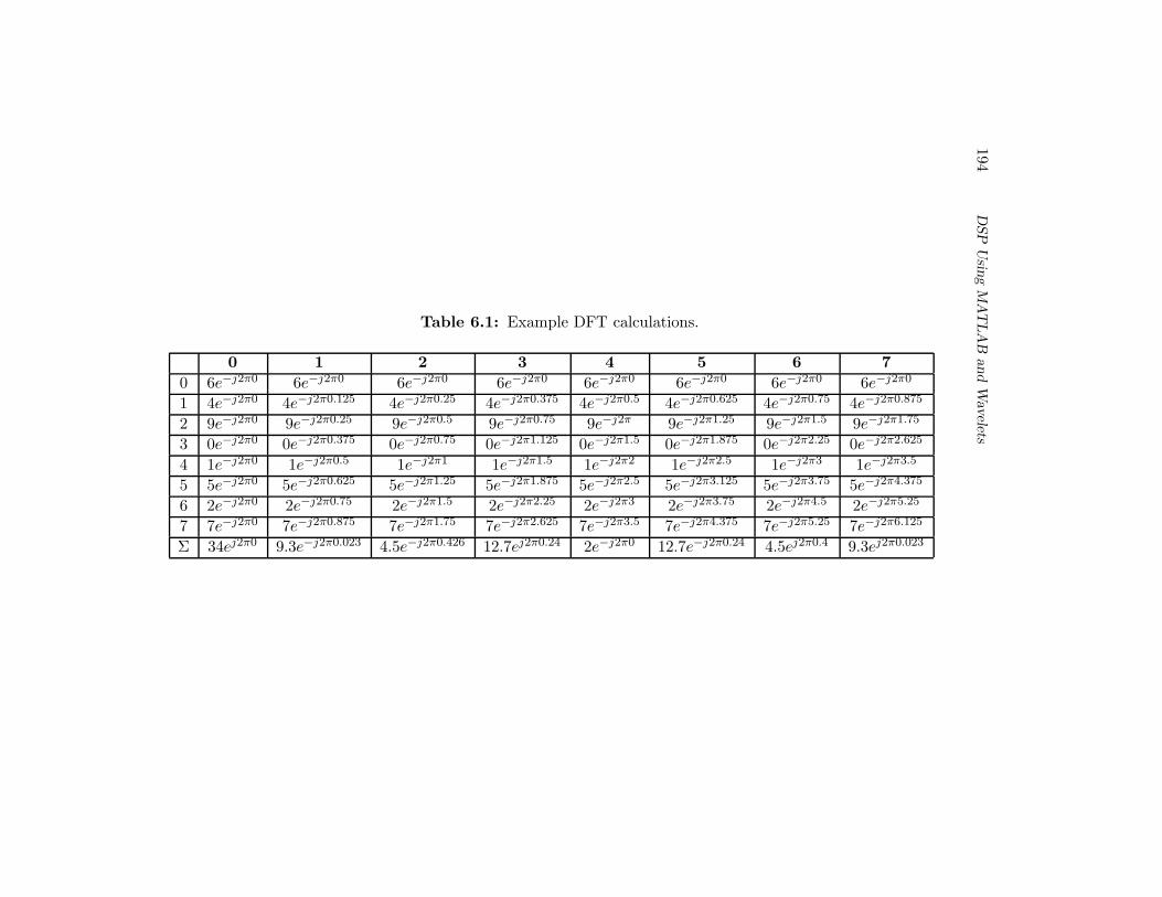
194D
SP
Usin
gM
AT
LA
Band
Wavelets
Table 6.1: Example DFT calculations.
0 1 2 3 4 5 6 7
0 6e−j2π0 6e−j2π0 6e−j2π0 6e−j2π0 6e−j2π0 6e−j2π0 6e−j2π0 6e−j2π0
1 4e−j2π0 4e−j2π0.125 4e−j2π0.25 4e−j2π0.375 4e−j2π0.5 4e−j2π0.625 4e−j2π0.75 4e−j2π0.875
2 9e−j2π0 9e−j2π0.25 9e−j2π0.5 9e−j2π0.75 9e−j2π 9e−j2π1.25 9e−j2π1.5 9e−j2π1.75
3 0e−j2π0 0e−j2π0.375 0e−j2π0.75 0e−j2π1.125 0e−j2π1.5 0e−j2π1.875 0e−j2π2.25 0e−j2π2.625
4 1e−j2π0 1e−j2π0.5 1e−j2π1 1e−j2π1.5 1e−j2π2 1e−j2π2.5 1e−j2π3 1e−j2π3.5
5 5e−j2π0 5e−j2π0.625 5e−j2π1.25 5e−j2π1.875 5e−j2π2.5 5e−j2π3.125 5e−j2π3.75 5e−j2π4.375
6 2e−j2π0 2e−j2π0.75 2e−j2π1.5 2e−j2π2.25 2e−j2π3 2e−j2π3.75 2e−j2π4.5 2e−j2π5.25
7 7e−j2π0 7e−j2π0.875 7e−j2π1.75 7e−j2π2.625 7e−j2π3.5 7e−j2π4.375 7e−j2π5.25 7e−j2π6.125
Σ 34ej2π0 9.3e−j2π0.023 4.5e−j2π0.426 12.7ej2π0.24 2e−j2π0 12.7e−j2π0.24 4.5ej2π0.4 9.3ej2π0.023

The
Fourier
Tra
nsfo
rm195
Table 6.2: Example DFT calculations (rectangular form).
0 1 2 3 4 5 6 7
0 6.0 + 0.0j 6.0 + 0.0j 6.0 + 0.0j 6.0 + 0.0j 6.0 + 0.0j 6.0 + 0.0j 6.0 + 0.0j 6.0 + 0.0j
1 4.0 + 0.0j 2.8 - 2.8j 0.0 - 4.0j -2.8 - 2.8j -4.0 - 0.0j -2.8 + 2.8j -0.0 + 4.0j 2.8 + 2.8j
2 9.0 + 0.0j 0.0 - 9.0j -9.0 - 0.0j -0.0 + 9.0j 9.0 + 0.0j 0.0 - 9.0j -9.0 - 0.0j -0.0 + 9.0j
3 0.0 + 0.0j 0.0 + 0.0j 0.0 + 0.0j 0.0 + 0.0j 0.0 + 0.0j 0.0 + 0.0j 0.0 + 0.0j 0.0 + 0.0j
4 1.0 + 0.0j -1.0 - 0.0j 1.0 + 0.0j -1.0 - 0.0j 1.0 + 0.0j -1.0 - 0.0j 1.0 + 0.0j -1.0 - 0.0j
5 5.0 + 0.0j -3.5 + 3.5j 0.0 - 5.0j 3.5 + 3.5j -5.0 - 0.0j 3.5 - 3.5j -0.0 + 5.0j -3.5 - 3.5j
6 2.0 + 0.0j -0.0 + 2.0j -2.0 - 0.0j 0.0 - 2.0j 2.0 + 0.0j -0.0 + 2.0j -2.0 - 0.0j -0.0 - 2.0j
7 7.0 + 0.0j 4.9 + 4.9j -0.0 + 7.0j -4.9 + 4.9j -7.0 - 0.0j -4.9 - 4.9j -0.0 - 7.0j 4.9 - 4.9j
Σ 34.0 + 0.0j 9.2 - 1.3j -4.0 - 2.0j 0.8 + 12.7j 2.0 - 0.0j 0.8 - 12.7j -4.0 + 2.0j 9.2 + 1.3j

196 DSP Using MATLAB and Wavelets
fanalysis[m] =mfsampling
N.
6.3 Plotting the Spectrum
To get a spectral plot, we will start out with an example signal. The following codesets up a signal, x.
>> % Set up an example signal
>> n = 0:99; % number of points
>> fs = 200; % sampling frequency
>> Ts = 1/fs; % sampling period
>> % x is our example signal
>> x = cos(2*pi*20*n*Ts + pi/4) + ...
3*cos(2*pi*40*n*Ts - 2*pi/5) + ...
2*cos(2*pi*60*n*Ts + pi/8);
>>
Now we need the frequency information from x, which we can get from theFourier transform. Also, we will establish the index m.
>> X = fft(x);
>> m = 0:length(X)-1;
It may be helpful to know the frequency resolution; the following code displaysit.
>> disp(sprintf('Freq resolution is every %5.2f Hz',...
fs/length(X)));
Freq resolution is every 2.00 Hz
>>
To see the spectrum, we will show both the frequency magnitude response anda plot of the phase angles.
>> % Plot magnitudes
>> subplot(2,1,1);
>> stem(m*fs/length(X),abs(X), 'b');
>> ylabel('magnitude');

The Fourier Transform 197
>> xlabel('frequency (Hz)');
>> title('Frequency magnitude response');
>> % Plot phase angles
>> subplot(2,1,2);
>> stem(m*fs/length(X),angle(X), 'b');
>> ylabel('phase angle');
>> xlabel('frequency (Hz)');
>> title('Phase angle plot');
When we run the previous code, we see the graphs as shown in Figure 6.5, andclearly there is frequency content at 20 Hz, 40 Hz, and 60 Hz, with magnitudes of 50,150, and 100, corresponding to relative magnitudes of 1, 3, and 2 as in our originalsignal. We notice a few annoying things about this figure, though. First, since theoriginal signal x is real, the frequency magnitude response has a mirror image, sowe only really need the first half of it. For the phases, the pattern is also reflectedaround the x-axis, so again we only need half of the plot. The phase plot containsa lot of information, actually too much. At frequency 80 Hz, for example, we seethat the amplitude approximates zero, while the phase angle is relatively large. (Weexpect the phase angles to be between −π and +π.)
To solve the first problem, we will simply plot the first half of both the magni-tudes and phases. We can set up a variable called half m to give us half the rangeof m, and use it in place of m. But when we use it, we must be careful to add 1 toit before using it as an array offset, since it starts at 0.
half_m = 0:ceil(length(X)/2);
stem(half_m*fs/length(X),abs(X(half_m+1)), 'b');
For the second problem, we need a little more information.
>> X(2)
ans =
-1.6871e-13 - 2.2465e-15i
>> angle(X(2))
ans =
-3.1283

198 DSP Using MATLAB and Wavelets
Figure 6.5: Spectrum for an example signal.

The Fourier Transform 199
>> abs(X(2))
ans =
1.6873e-13
The above commands confirm our suspicion that the phase angles are calculatedand shown for every X value even when they are close to zero. Fixing this requiresthe use of a tolerance value. If the magnitude is smaller than the tolerance, thenwe should assume a zero phase. After all, the magnitudes correspond to how mucha sinusoid contributes to our signal. If a sinusoid contributes about zero, then itmakes no sense to keep a nonzero phase angle for it.
>> % The next 3 lines allow us to ignore phases
>> % that go with very small magnitudes.
>> tolerance = 0.00001;
>> X2 = ceil(abs(X) - tolerance);
>> X3 = round(X2 ./ (X2+1));
>> % X3 above is a vector of 0s and 1s
The above commands may be a bit confusing, but these lines set up a binaryvector. The subtraction operation separates the magnitudes for us; since all mag-nitudes are positive, any negative values after the subtraction correspond to phasesthat we should ignore, and the ceil function will make them zero. Now the problemis to map the nonzero values in X2 to 1. Dividing each value of X2 by itself (plus1) will return values that are either 0 or almost 1, while avoiding a divide-by-zeroerror. The round function simply takes care of making the “almost 1” values equalto 1. The code results in vector X3, consisting of zeros for the phases to ignore, andones for the phases we want to see. We can then use it in the stem plot below, tozero-out any phases with magnitudes close to zero. The following plot does not usehalf m as above, but we can put all of this together.
subplot(2,1,2);
stem(m*fs/length(X),angle(X).*X3, 'b');
Now we can put all of this together into a program, to plot the spectrum. Whenwe run this program, we get the graphs shown in Figure 6.6, with the magnitudesand phase angles plotted versus the frequencies.

200 DSP Using MATLAB and Wavelets
Figure 6.6: Improved spectrum for an example signal.

The Fourier Transform 201
This program is shown in its entirety, since its pieces are shown above. Tosummarize what it does, first it makes an example signal by adding several sinusoids.Next, it finds the Fourier transform, then prints the frequency resolution. After this,it plots the magnitudes. It also plots the phases, but first it zeros-out the phasesthat have a tiny corresponding magnitude.
% spectrum.m
%
% Show the spectrum of an example signal.
%
% Set up an example signal
n = 0:99; % number of points
fs = 200; % sampling frequency
Ts = 1/fs; % sampling period
% x is our example signal
x = cos(2*pi*20*n*Ts + pi/4) + ...
3*cos(2*pi*40*n*Ts - 2*pi/5) + ...
2*cos(2*pi*60*n*Ts + pi/8);
% Find the spectrum
X = fft(x);
%m = 0:length(X)-1;
half_m = 0:ceil(length(X)/2);
disp(sprintf('Freq resolution is every %5.2f Hz',...
fs/length(X)));
% Plot magnitudes
subplot(2,1,1);
%stem(m*fs/length(X),abs(X), 'b');
stem(half_m*fs/length(X),abs(X(half_m+1)), 'b');
ylabel('magnitude');
xlabel('frequency (Hz)');
title('Frequency magnitude response');
% Plot phase angles
subplot(2,1,2);
% The next 3 lines allow us to ignore phases
% that go with very small magnitudes.
tolerance = 0.00001;

202 DSP Using MATLAB and Wavelets
X2 = ceil(abs(X) - tolerance);
X3 = round(X2 ./ (X2+1));
% X3 above is a vector of 0s and 1s
%stem(m*fs/length(X),angle(X).*X3, 'b');
stem(half_m*fs/length(X), ...
angle(X(half_m+1)).*X3(half_m+1), 'b');
ylabel('phase angle');
xlabel('frequency (Hz)');
title('Phase angle plot');
6.4 Zero Padding
When we zero-pad a signal in the time-domain, we get a smoother-looking fre-quency resolution. Why does this happen? Actually, the length of the sampledsignal determines the frequency resolution, and zero-padding does not add any newinformation. Though the zero-padded signal results in a more visually appealingfrequency-domain representation, it does not add to the resolution of the transform.
Why can we zero-pad our time-domain signal? Part of the explanation hasto do with the continuous Fourier transform. For convenience, we use the radianfrequency, ω = 2πf . Using ω also allows us to use f(t) for our function’s name,without confusing it with frequency.
F (ω) =
∫ ∞
−∞f(t)e−jωtdt
Suppose f(t) is a signal that has zero value outside the interval [a, b], and assumea < b < c. We can, therefore, replace the previous equation with the following:
F (ω) =
∫ c
af(t)e−jωtdt
=
∫ b
af(t)e−jωtdt+
∫ c
bf(t)e−jωtdt.
Since f(t) = 0 outside the interval [a, b] by definition, the second integral evalu-ates to 0. We can add 0 to the righthand side of the equation,
F (ω) = 0 +
∫ b
af(t)e−jωtdt.
Therefore, for continuous signals, F (ω) is the same whether or not we consider

The Fourier Transform 203
f(t) outside of its support. For a discrete signal, the number of points for thefrequency-domain signal equals the number of points in the time-domain signal, soadding zeros means that there will be more frequency-domain points. The analysisfrequencies, as a result, become finer since they are closer together.
6.5 DFT Shifting Theory
There is a DFT shifting theory, stating that sampling a signal will give the sameresults (in terms of frequency magnitude response), even when the samples areshifted, such as removing the first k samples and appending them to the end ofthe sample sequence. This is an important theory, since it tells us that there is nocritical time to start recording samples. The program below demonstrates this idea.Notice how the plot command puts two signals on the graph at the same time, onein blue (’b’) and the other in green (’g’). Try other colors like red (’r’) and black(’k’).
% Demonstrate DFT Shifting theory
%
% parameters to modify
number_of_samples = 16;
shift = 3; % Must be less than number_of_samples
fs = 2000; % sampling frequency
% Make our example signal
Ts = 1/fs;
range = 1:number_of_samples;
x(range) = 2*cos(2*pi*400*(range-1)*Ts) ...
+ cos(2*pi*700*(range-1)*Ts);
% Make y a shifted version of x
y = [x(shift:number_of_samples), x(1:shift-1)];
% Get fft of each signal
X = fft(x);
Y = fft(y);
% Find magnitudes

204 DSP Using MATLAB and Wavelets
Xmag = abs(X);
Ymag = abs(Y);
% Find phase angles
Xphase = angle(X);
Yphase = angle(Y);
% Show results in a graph
subplot(3,1,1), plot(range, x,'bd', range, y,'g*');
mystr = strcat('original (blue diamond) and shifted', ...
'(green *) versions of the sampled signal');
title(mystr);
subplot(3,1,2), plot(range, Xmag,'bd', range, Ymag,'k*');
title('Xmagnitude = diamond, Ymagnitude = *');
subplot(3,1,3), plot(range, Xphase,'bd', range, Yphase,'k*');
title('Xphase = diamond, Yphase = *');
Figure 6.7 shows what the output for this program looks like. Though the phaseangles are different, the frequency magnitudes are the same for the original as wellas the shifted signal. We should expect the phase angles to be different, sincethese values determine how a composite signal “lines up” with with the samples.Otherwise, we would not be able to get the original signals back via the inversetransform.
6.6 The Inverse Discrete Fourier Transform
This is the Inverse Discrete Fourier Transform (IDFT):
x[n] =1
N
N−1∑
m=0
X[m](cos(2πnm/N) + j sin(2πnm/N))
where n = 0..N − 1. Notice how similar it is to the DFT, the main differencesbeing the 1/N term, and the plus sign in front of the complex part. The plus signis no coincidence, the inverse transform works by using what we call the complexconjugate of the forward transform. A complex conjugate, stated simply, occurswhen the complex part has a negated sign. For example, 4 − j2 and 4 + j2 arecomplex conjugates. A superscripted asterisk denotes complex conjugation. If wesay a = 3 + j7 and b = 3 − j7, then we could also say a = b∗ or b = a∗.
An alternate form of the IDFT follows, using Euler’s formula to replace thesinusoids with exponentials.

The Fourier Transform 205
0 2 4 6 8 10 12 14 16−4
−2
0
2
4original (diamond) and shifted(*) versions of the sampled signal
0 2 4 6 8 10 12 14 160
5
10
15
20Xmagnitude = diamond, Ymagnitude = *
0 2 4 6 8 10 12 14 16−4
−2
0
2
4Xphase = diamond, Yphase = *
Figure 6.7: Example output of DFT-shift program.
x[n] =1
N
N−1∑
m=0
X[m]ej2πnm/N
Below is a MATLAB function that calculates the Inverse Discrete Fourier Trans-form (IDFT). Like the DFT program above, this program intends only to demon-strate how the IDFT can be calculated. MATLAB has an ifft function that givesthe same results, only faster.
function [x] = idft(X)
% Find the 1D Inverse DFT of an input signal.
% It returns the IDFT of the signal as a
% vector of complex numbers.
%
% Usage:
% [x] = idft(X);
%
% This function is NOT very efficient,

206 DSP Using MATLAB and Wavelets
% but it demonstrates how the IDFT is done.
Xsize = length(X);
% Do reconstruction
for n=0:Xsize-1
for m=0:Xsize-1
arra(n+1,m+1) = X(m+1) * (cos(2*pi*m*n/Xsize) + ...
j*sin(2*pi*m*n/Xsize));
end
end
for n=0:Xsize-1
mysumm = 0;
for m=0:Xsize-1
mysumm = mysumm + arra(n+1,m+1);
end
% Keep only the real part
%x(n+1) = real(mysumm) / Xsize;
x(n+1) = mysumm / Xsize;
end
Below is shown a MATLAB session that demonstrates the DFT and IDFT func-tions. First, the signal mysignal is given some example values. Next, the “dft”function is called. Notice that the “dft” function will return three values, but herewe only use the first.
After the DFT values are stored in variable M, the inverse discrete Fourier trans-form is computed, and stored in mysignal 2. This signal should have the sameinformation as mysignal, and this is shown to be true. The round function gets ridof the part beyond the decimal point, and the real function ignores the imaginarypart (which is zero).
To get started, select "MATLAB Help" from the Help menu.
>> mysignal = [ 7 4 3 9 0 1 5 2 ];
>> M = dft(mysignal)
M =
Columns 1 through 6

The Fourier Transform 207
31.0000 4.1716 - 5.0711i -1.0000 + 6.0000i
9.8284 - 9.0711i -1.0000 - 0.0000i 9.8284 + 9.0711i
Columns 7 through 8
-1.0000 - 6.0000i 4.1716 + 5.0711i
>> mysignal_2 = idft(M)
mysignal_2 =
Columns 1 through 6
7.0000 + 0.0000i 4.0000 + 0.0000i 3.0000 - 0.0000i
9.0000 - 0.0000i 0.0000 - 0.0000i 1.0000 + 0.0000i
Columns 7 through 8
5.0000 + 0.0000i 2.0000 + 0.0000i
>> real(round(mysignal_2))
ans =
7 4 3 9 0 1 5 2
>> mysignal
mysignal =
7 4 3 9 0 1 5 2
6.7 Forward and Inverse DFT
This section shows that when we take a signal, perform the DFT on it, and thenperform the IDFT on the result, we will end up with the same values that we startedwith. We will begin by remembering the formulas.

208 DSP Using MATLAB and Wavelets
Discrete Fourier Transform (DFT):
X[m] =
N−1∑
n=0
x[n]e−j2πnm/N
where m = 0..N − 1.Inverse Discrete Fourier Transform (IDFT):
x[n] =1
N
N−1∑
m=0
X[m]ej2πnm/N
where n = 0..N − 1.Let’s start with an example signal, x = x0, x1, x2, x3. We can find the DFT of
x using the general formulas above, and since we know that N = 4, we can replaceit in the formula.
X[m] =
3∑
n=0
x[n]e−j2πnm/4
X[m] = x0e−j2π0m/4 + x1e
−j2π1m/4 + x2e−j2π2m/4 + x3e
−j2π3m/4
We can then find the inverse transform...
x[n] =1
4
3∑
m=0
X[m]ej2πnm/4
x[n] =1
4(X[0]ej2πn0/4 +X[1]ej2πn1/4 +X[2]ej2πn2/4 +X[3]ej2πn3/4)
...and replace the X[m] terms with their equivalents.
x[n] =1
4((x0e
−j2π0×0/4 + x1e−j2π1×0/4 + x2e
−j2π2×0/4 + x3e−j2π3×0/4)ej2πn0/4+
(x0e−j2π0×1/4 + x1e
−j2π1×1/4 + x2e−j2π2×1/4 + x3e
−j2π3×1/4)ej2πn1/4+
(x0e−j2π0×2/4 + x1e
−j2π1×2/4 + x2e−j2π2×2/4 + x3e
−j2π3×2/4)ej2πn2/4+
(x0e−j2π0×3/4 + x1e
−j2π1×3/4 + x2e−j2π2×3/4 + x3e
−j2π3×3/4)ej2πn3/4)

The Fourier Transform 209
Combining the exponents:
x[n] =1
4((x0e
−j2π0×0/4+j2πn0/4 + x1e−j2π1×0/4+j2πn0/4+
x2e−j2π2×0/4+j2πn0/4 + x3e
−j2π3×0/4+j2πn0/4)+
(x0e−j2π0×1/4+j2πn1/4 + x1e
−j2π1×1/4+j2πn1/4+
x2e−j2π2×1/4+j2πn1/4 + x3e
−j2π3×1/4+j2πn1/4)+
(x0e−j2π0×2/4+j2πn2/4 + x1e
−j2π1×2/4+j2πn2/4+
x2e−j2π2×2/4+j2πn2/4 + x3e
−j2π3×2/4+j2πn2/4)+
(x0e−j2π0×3/4+j2πn3/4 + x1e
−j2π1×3/4+j2πn3/4+
x2e−j2π2×3/4+j2πn3/4 + x3e
−j2π3×3/4+j2πn3/4)).
Multiplying out the terms:
x[n] =1
4((x0e
j2π(−0×0+n0)/4 + x1ej2π(−1×0+n0)/4+
x2ej2π(−2×0+n0)/4 + x3e
j2π(−3×0+n0)/4)+
(x0ej2π(−0×1+n1)/4 + x1e
j2π(−1×1+n1)/4+
x2ej2π(−2×1+n1)/4 + x3e
j2π(−3×1+n1)/4)+
(x0ej2π(−0×2+n2)/4 + x1e
j2π(−1×2+n2)/4+
x2ej2π(−2×2+n2)/4 + x3e
j2π(−3×2+n2)/4)+
(x0ej2π(−0×3+n3)/4 + x1e
j2π(−1×3+n3)/4+
x2ej2π(−2×3+n3)/4 + x3e
j2π(−3×3+n3)/4)).
Simplifying:
x[n] =1
4((x0e
j2π0/4 + x1ej2π0/4 + x2e
j2π0/4 + x3ej2π0/4)+
(x0ej2π(n)/4 + x1e
j2π(n−1)/4 + x2ej2π(n−2)/4 + x3e
j2π(n−3)/4)+
(x0ej2π(2n)/4 + x1e
j2π(2n−2)/4 + x2ej2π(2n−4)/4 + x3e
j2π(2n−6)/4)+
(x0ej2π(3n)/4 + x1e
j2π(3n−3)/4 + x2ej2π(3n−6)/4 + x3e
j2π(3n−9)/4)).

210 DSP Using MATLAB and Wavelets
Simplifying even more (ej0 = 1):
x[n] =1
4((x0 + x1 + x2 + x3)+
(x0ej2π(n)/4 + x1e
j2π(n−1)/4 + x2ej2π(n−2)/4 + x3e
j2π(n−3)/4)+
(x0ej2π(2n)/4 + x1e
j2π(2n−2)/4 + x2ej2π(2n−4)/4 + x3e
j2π(2n−6)/4)+
(x0ej2π(3n)/4 + x1e
j2π(3n−3)/4 + x2ej2π(3n−6)/4 + x3e
j2π(3n−9)/4)).
Let’s see what we get when n = 1:
x[1] =1
4((x0 + x1 + x2 + x3)+
(x0ej2π(1)/4 + x1e
j2π(0)/4 + x2ej2π(−1)/4 + x3e
j2π(−2)/4)+
(x0ej2π(2)/4 + x1e
j2π(0)/4 + x2ej2π(−2)/4 + x3e
j2π(−4)/4)+
(x0ej2π(3)/4 + x1e
j2π(0)/4 + x2ej2π(−3)/4 + x3e
j2π(−6)/4)).
Remember that these exponential values, such as 2π(−6)/4, correspond to angles,and any angle greater than 2π can have an integer multiple of 2π removed from it.For example, ej2π(−6)/4 = e−j12π/4 = e−j3π = e−j(2π+π) = e−jπ.
x[1] =1
4((x0 + x1 + x2 + x3)+
(x0ejπ/2 + x1 + x2e
−jπ/2 + x3e−jπ)+
(x0ejπ + x1 + x2e
−jπ + x3e−j2π)+
(x0ejπ3/2 + x1 + x2e
−jπ3/2 + x3e−jπ))
Next, we will replace the exponentials with sinusoids, using Euler’s formula.
x[1] =1
4((x0 + x1 + x2 + x3)+
(x0(cos(π/2)+ j sin(π/2))+x1 +x2(cos(π/2)− j sin(π/2))+x3(cos(π)− j sin(π)))+
(x0(cos(π) + j sin(π)) + x1 + x2(cos(π) − j sin(π)) + x3(cos(2π) − j sin(2π)))+
(x0(cos(3π/2)+j sin(3π/2))+x1+x2(cos(3π/2)−j sin(3π/2))+x3(cos(π)−j sin(π))))
Now, we can calculate the sinusoids (Table 6.3), and plug in the values.

The Fourier Transform 211
Table 6.3: Sinusoids that simplify things for us.
cos(π/2) = 0, sin(π/2) = 1cos(π) = −1, sin(π) = 0cos(2π) = 1, sin(2π) = 0cos(3π/2) = 0, sin(3π/2) = −1
x[1] =1
4((x0 + x1 + x2 + x3)+
(x0(j) + x1 + x2(−j) + x3(−1 − j0))+
(x0(−1 + j0) + x1 + x2(−1 − j0) + x3(1 − j0))+
(x0(j(−1)) + x1 + x2(−j(−1)) + x3(−1 − j0)))
Simplifying:
x[1] =1
4((x0 + x1 + x2 + x3)+
(x0(j) + x1 + x2(−j) + x3(−1))+
(x0(−1) + x1 + x2(−1) + x3(1))+
(x0(−j) + x1 + x2(j) + x3(−1))).
Grouping terms:
x[1] =1
4(x0(1 + j− 1− j) +x1(1 +1 +1 +1) +x2(1− j − 1 + j) + x3(1− 1 +1− 1))
x[1] =1
4(x0(0) + x1(4) + x2(0) + x3(0))
x[1] = x1.
Thus, the inverse transform gives us back the data that we had before the forwardtransform. The 1
N term appears in the inverse transform to scale the outputs backto the original magnitude of the inputs. We only show this for one of the originalvalues, but the interested reader should be able to verify that this works for all fourof the original values.

212 DSP Using MATLAB and Wavelets
6.8 Leakage
The DFT does not have infinite resolution. A consequence of this is that sometimesfrequencies that are present in a signal are not sharply defined in the DFT, andthe frequency’s magnitude response appears to be spread out over several analysisfrequencies. This is called DFT leakage. The following code demonstrates this. Inthe code below, we simulate two sampled signals: x1 and x2. If you look closely,you will see that the equations defining these two signals are the same. What wechange are the parameters; the sampling frequencies (fs1 and fs2), which alter thesampling periods (Ts1 and Ts2), and the number of samples to read (given by thelengths of n1 and n2).
fs1 = 1000; fs2 = 1013;
Ts1 = 1/fs1; Ts2 = 1/fs2;
n1 = 0:99; n2 = 0:98;
x1 = 3*cos(2*pi*200*n1*Ts1 - 7*pi/8) + 2*cos(2*pi*300*n1*Ts1) ...
+ cos(2*pi*400*n1*Ts1 + pi/4);
x2 = 3*cos(2*pi*200*n2*Ts2 - 7*pi/8) + 2*cos(2*pi*300*n2*Ts2) ...
+ cos(2*pi*400*n2*Ts2 + pi/4);
mag1 = abs(fft(x1));
mag2 = abs(fft(x2));
The results are shown in the following graphs. When we take 100 samples ofsignal x at 1000 samples per second, we get the spectral plot shown in Figure 6.8.
x(t) = 3 cos(2π200t − 7π/8) + cos(2π300t) + 2 cos(2π400t + π/4)
It shows what happens when the analysis frequencies happen to match up nicelywith the frequencies present in the signal. The second figure represents the samesignal, only with the number of samples N , and the sampling frequency fs changedto 99 samples at 1013 samples per second, Figure 6.9. Since
fanalysis[m] = mfs/N,
changing either (or both) of these parameters affects the analysis frequencies usedin the DFT. For the second figure, the analysis frequencies do not match up withthe frequencies of the signal, so we see the spectral content spread across ALLfrequencies. The signal has not changed, but our view of the frequency information

The Fourier Transform 213
has. A trained individual would interpret the second figure as if it were the firstfigure, however.
0 10 20 30 40 50 60 70 80 90 1000
50
100
150
200
frequency spectrum (m), freqs = m*1000/100
DFT leakage: 3cos(2pi200t − 7pi/8) + 2cos(2pi300t) + cos(2pi400t + pi/4)
Figure 6.8: Frequency content appears at exact analysis frequencies.
0 10 20 30 40 50 60 70 80 90 1000
20
40
60
80
100
120
frequency spectrum (m), freqs = m*1013/99
Figure 6.9: Frequency content appears spread out over analysis frequencies.
A window is a way of modifying the input signal so that there are no suddenjumps (discontinuities) in it. Even if you do not use a window function, when yousample a signal, you impose a rectangular window function on it [11]. In otherwords, the input is considered 0 for all values before you start sampling and allvalues after you stop. The sudden jumps (discontinuities) show up in the frequencyresponse as the sinc function. Leakage occurs when the analysis frequencies do not

214 DSP Using MATLAB and Wavelets
land on the actual frequencies present. This means that the actual information“leaks” into other DFT output bins; it shows up as other frequencies. Windowingreduces the sidelobes of the sinc function (of the Continuous Fourier Transform, orCFT for short), which in turn decreases the effect of leakage, since the DFT is asampled version of the continuous Fourier transform [11].
In other words, looking at the CFT of a signal component (i.e., a single sinusoid),we see the sinc function. Looking at the CFT of a windowed version of the samesignal, we see a sinc function with lower sidelobe levels (though a wider main lobe).If we sample the CFT, we might be lucky and sample it right at the point betweensidelobes, so we have many zeros and a single spike. Realistically, our sampleswill land where we have one or two spikes, and several nonzero values, due to thesidelobes. The lower these sidelobes, the better our DFT indicates the frequenciesthat are actually present.
6.9 Harmonics and Fourier Transform
Harmonics and the Fourier transform are closely linked. Harmonics refers to theuse of sinusoids related by a fundamental frequency f0, that is, adding sinusoids offrequencies f0, 2f0, 3f0, etc.
The following program demonstrates harmonics. Its objective is to approximatea triangle wave with a sum of sinusoids. When we run it, we see that the approxi-mation gets better and better as more sinusoids are added. We use a fundamentalfrequency of 1 Hz. After creating signal x as a triangle wave, the program findsthe DFT of it using the fft command in MATLAB. Next, it finds the magnitudesand phases for all of the sinusoids corresponding to the DFT results. Finally, theprogram shows the sum of the sinusoids, pausing briefly between iterations of theloop to show the progress. Essentially, this performs the inverse DFT. Figure 6.10shows what the progress looks like about one-sixth of the way through (the solid lineis the original signal, and the sum of sinusoids is shown as a dash-dot line). Runningthe program to completion shows that the final approximation appears directly overtop of the original signal.
%
% Show how the DFT function can represent a triangle wave
%
% first, make a triangle wave
for i=1:20
x(i) = i;

The Fourier Transform 215
0 10 20 30 40 50 60 70 80 900
2
4
6
8
10
12
14
16
18
20
Figure 6.10: Approximating a triangle wave with sinusoids.
end
k=20;
for i=21:40
k=k-1;
x(i) = k;
end
for i=41:60
x(i) = i-40;
end
k=20;
for i=61:80
k=k-1;
x(i) = k;
end
% OK, now we have the triangle wave as signal x
% Find the DFT of it, and scale the result.
% In other words, represent signal x as a sum of sinusoids
[y] = fft(x);
% Scale the result, so that it is the same size as original
y = y / length(x);
% Convert to polar coordinates (magnitudes and phases)
mag = abs(y);
phi = angle(y);

216 DSP Using MATLAB and Wavelets
% Now, reconstruct it.
% This shows what the "sum of sinusoids" version looks like
t=0:(1/length(mag)):1;
f = 1; % Our fundamental frequency is 1, since time t=n*m/N
a = 0;
% Show it, adding another sinusoid each time
for k=0:length(mag)-1
a=a+mag(k+1)*(cos(2*pi*f*k*t+phi(k+1)) ...
+ j*sin(2*pi*f*k*t+phi(k+1)));
plot(1:length(x), x, 'r', 1:length(a), real(a), 'b-.')
pause(0.1);
end
The first thing this program does is create a signal to work with; a trianglewave. Below, we show how the program works with a square wave. Note the finalfor loop, enclosing plot and pause commands. We could use the “plotharmonic”function instead, but this program shows the reconstruction of the original signal asa step-by-step process.
Try the above program again, replacing the triangle wave above (program lines5–22) with the following signals. It is a good idea to type clear all between them.
% Make a saw-tooth wave
for i=1:40
x(i) = i;
end
for i=41:80
x(i) = i-40;
end
% Now we have the saw-tooth wave as signal x
The progress of the approximation (one-sixth of the way) appears in Figure 6.11.This figure also shows the result when all terms are used. Notice that the biggestdifference between the original and the approximation is the final point. The sinusoidapproximation anticipates that the pattern will repeat.
% Make a square wave
for i=1:20
x(i) = 0;
end
for i=21:40

The Fourier Transform 217
0 10 20 30 40 50 60 70 80 900
10
20
30
40Adding the first one−sixth of sinusoids
0 10 20 30 40 50 60 70 80 900
10
20
30
40
50Approximating with all sinusoids
Figure 6.11: Approximating a saw-tooth wave with sinusoids.
x(i) = 1;
end
for i=41:60
x(i) = 0;
end
for i=61:80
x(i) = 1;
end
% Now we have the square wave as signal x
Figure 6.12 shows the approximation of the previous square wave for one-sixthof sinusoids as well as all sinusoids.
% Make a combination saw-tooth square wave
for i=1:40
x(i) = i;
end
for i=41:80
x(i) = 40; %i-40;
end
% repeat
for i=81:120
x(i) = i-80;
end
for i=121:160

218 DSP Using MATLAB and Wavelets
0 10 20 30 40 50 60 70 80 900
0.2
0.4
0.6
0.8
1Adding the first one−sixth of sinusoids
0 10 20 30 40 50 60 70 80 90−0.2
0
0.2
0.4
0.6
0.8
1
1.2Approximating with all sinusoids
Figure 6.12: Approximating a square wave with sinusoids.
x(i) = 40; %40;
end
Figure 6.13 shows the approximation of a combined sawtooth-square wave foruse of one-sixth of the terms as well as all terms.
0 20 40 60 80 100 120 140 160 1800
10
20
30
40Adding the first one−sixth of sinusoids
0 20 40 60 80 100 120 140 160 1800
10
20
30
40
50Approximating with all sinusoids
Figure 6.13: Approximating a saw-tooth square wave with sinusoids.
The DFT versions of the signals are good, but they are not perfect. Discontinu-ities in signals, such as the quick rise and quick fall of the square wave, are difficultto represent in the frequency-domain. The simple impulse function demonstratesthis. It is very easy to represent in the time-domain:

The Fourier Transform 219
x(t) = 1, t = 0
x(t) = 0, otherwise.
But to represent this in the frequency-domain, we need an infinite number ofsinusoids.
Looking at this problem the other way, consider a simple sinusoid. In thefrequency-domain, it is easily represented as a spike of half-amplitude at the pos-itive and negative frequencies (recall the inverse Euler’s formula). For all otherfrequencies, it is zero. If we want to represent this same signal in time, we haveamplitude × cos(2πft + φ), which gives us a function value for any value of time.Recording this signal’s value for every value of time would require writing down aninfinite number of terms.
This leads us to the observation that what is well-defined in the time-domainis poorly represented in the frequency-domain. Also, what is easy to represent inthe frequency domain is difficult to represent in the time-domain. In effect, this isWerner Heisenberg’s uncertainty principle [23].
6.10 Sampling Frequency and the Spectrum
As we saw with the DFT, when we sample a real signal at a rate of fs sam-ples/second, the frequency magnitude plot from fs/2 to fs looks like a mirror imageof 0 to fs/2.
A real signal is made up of components such as cos(θ), or can be put in this form.If it were a complex signal, there would be a j sin(θ) component, or something that
can be put in that form (such as a j cos(θ) component). Since cos(θ) = ejθ
2 + e−jθ
2 , areal signal always has a positive and negative frequency component on the spectrumplot.
Given cos(θ) = ejθ
2 + e−jθ
2 , and given Euler’s law:
ejθ = cos(θ) + j sin(θ)
ejθ =ejθ
2+e−jθ
2+ j sin(θ)
ejθ
2=e−jθ
2+ j sin(θ)

220 DSP Using MATLAB and Wavelets
j sin(θ) =ejθ
2− e−jθ
2.
This means that a complex signal has two frequency components as well. Of course,if we had a signal such as cos(θ) + j sin(φ), we would have:
cos(θ) + j sin(φ) =ejθ
2+e−jθ
2+ejφ
2− e−jφ
2.
If θ equals φ, thencos(θ) + j sin(θ) = ejθ.
For this reason, we concern ourselves with only the first half of the frequencyresponse. When it looks like Figure 6.14, we say it is a lowpass filter. This meansthat any low-frequency (slowly changing) components will remain after the signalis operated on by the system. High-frequency components will be attenuated, or“filtered out.” When it looks like Figure 6.15, we say it is a highpass filter. Thismeans that any high-frequency (quickly changing) components will remain after thesignal is operated on by the system.
fs2
1
Figure 6.14: Frequency response of a lowpass filter.
The frequency response can be found by performing the DFT on a system’soutput when the impulse function is given as the input. This is also called the“impulse response” of the system. To get a smoother view of the frequency response,the impulse function can be padded with zeros.
fs2
1
Figure 6.15: Frequency response of a highpass filter.
The more samples that are in the input function to the DFT, the better theresolution of the output will be.
The Fourier Transform 221
Exercise:w[n] = x[n] + x[n− 1]
y[n] = x[n] − x[n− 1]
Find and plot the frequency response for w and y.
First, assume x is a unit impulse function, and find w[n] and y[n]. Pad thesesignals, say up to 128 values, so that the result will appear smooth. Next, find theDFT (or FFT) of w and y, and plot the magnitudes of the result. The plots shouldgo to only half of the magnitudes, since the other half will be a mirror image.
6.11 Summary
This chapter covers the Fourier transform, inverse Fourier transform, and relatedtopics. The Fourier transform gives frequency (spectral) content of a signal. Givenany series of samples, we can create a sum of sinusoids that approximate it, if notrepresent it exactly.
6.12 Review Questions
1. Suppose we were to sample a signal at fs = 5000 samples per second, and wewere to take 250 samples. After performing the DFT, we find that the first10 results are as follows. What does this say about the frequencies that arepresent in our input signal? (Assume that the other values for X[m] up tom = 125 are 0.)
X[m] = 10, 0, 0, 2 + j4, 0, 1, 0, 0, 0, 2 − j4
2. An input sequence, x[n], has the Fourier transform performed on it. The resultis:X[m] = 3, 2+j4, 1, 5-j3, 0, 0, 0, 5+j3, 1, 2-j4.
a. Find (and plot) the magnitudes and phase angles.
b. You should notice some symmetry in your answer for the first part. What

222 DSP Using MATLAB and Wavelets
kind of symmetry do you expect (for the magnitudes), and why?
3. An input sequence, x[n], has the Fourier transform performed on it. The resultis:X[m] = 3, 2+j4, 1, 5-j3, 0, 0, 0, 5+j3, 1, 2-j4.Given that x[n] was sampled at fs = 100 samples per second,
a. What is the DC component for this signal?b. What frequencies are present in the input? Rank them in order accordingto amplitude.c. Using MATLAB, find x[n].
4. Given x2 = [0.4786,−1.0821,−0.5214,−0.5821,−0.2286, 1.3321, 0.7714, 0.8321];find (using MATLAB) the FFT values Xmagnitude[m] and Xphase[m] for m =0..7. Show all of your work. Also, graph your results.
5. Try a 5-tap FIR filter using the following random data. Note that this com-mand will return different values every time.
x = round(rand(1, 20)*100)
Use h1[k] = 0.5, 0.5, 0.5, 0.5, 0.5, and compare it to h2[k] = 0.1, 0.3, 0.5,0.3, 0.1, and h3[k] = 0.9, 0.7, 0.5, 0.7, 0.9. Graph the filter’s output, andits frequency magnitude response. Be sure to use the same x values. Makeone graph with the filters’ outputs, and another graph with the frequencyresponses. Judging each set of filter coefficients as a lowpass filter, which isbest? Which is worst? Why?
6. Try an 8-tap FIR filter using the following random data. Note that thiscommand will return different values every time.
x = round(rand(1, 20)*100)
Use h1[k] = 0.5, 0.5, 0.5, 0.5, 0.5, 0.5, 0.5, 0.5, and compare it to h2[k] =0.1, 0.2, 0.3, 0.5, 0.5, 0.3, 0.2, 0.1, and h3[k] = 0.9, 0.7, 0.6, 0.5, 0.5, 0.6,0.7, 0.1. Graph the filter’s output and its frequency magnitude response.Be sure to use the same x values. Make one graph with the filters’ outputs,and another graph with the frequency responses. Judging each set of filtercoefficients as a lowpass filter, which is best? Which is worst? Why?

The Fourier Transform 223
7. What is 3e−j2π0.2 in complex Cartesian coordinates? (That is, in the forma+ jb.) Hint: use Euler’s formula.
8. What is 1.7 − j3.2 in complex polar coordinates? (That is, in the form rejφ.)Hint: use the magnitude and angle calculations from Chapter 1, “Introduc-tion.”


Chapter 7
The Number e
Euler’s formula: so far we have used it like a transform to go from ej() to cos() +j sin(), or back. But why can we do this? Where does e come from? What doesj really mean? These questions and more will be answered in this chapter. Alongthe way, we have a few important concepts about DSP, including how a complexnumber can be thought of as a vector on the complex plane (instead of a real numberon the real number line), how such a vector can rotate, how we can go betweenalternate representations of the same information (such as polar coordinates versusCartesian ones), and how some representations are more suitable for mathematicalmanipulations than others.
7.1 Reviewing Complex Numbers
Instead of using the Cartesian coordinate system to map a variable and a function,we can represent a complex number as a point on this plane. Here we have thex-axis represent the “real” part of a complex number, and the y-axis represent the“imaginary” part of it. Of course, we can also think of this same information interms of polar coordinates; that is, we can represent it as a point (x, y), or as avector r∠θ (length and angle), Figure 7.1.
The x-position of the vector is given by the function x = r cos(θ), where r isthe radius (or length of the vector), and θ is the angle between the vector and thex-axis. The y-coordinate of the vector follows as y = r sin(θ). These functionscome from geometry, as Figure 7.2 shows. A 2D vector, with a vertical line segmenty units high, makes a right triangle with the x-axis.
Using the notation j, we can write the position of the vector as r cos(θ) +
225

226 DSP Using MATLAB and Wavelets
AAAABB
real axis
imaginary axis
j
θr
(x, y)
Figure 7.1: A complex number can be shown as a point or a 2D vector.
y = r sin( )θx = r cos( )θθ
ry
x
Figure 7.2: A vector forms a right triangle with the x-axis.

The Number e 227
j r sin(θ). Recall Euler’s formula,
ejθ = cos(θ) + j sin(θ)
or, multiplying by a constant,
r cos(θ) + j r sin(θ) = r ejθ
so we can substitute r ejθ to represent this vector (also called a phasor).Imagine that a 2D vector starts on the x-axis, and rotates counterclockwise
around the origin (see Figure 7.3). As it rotates, the length of the vector staysthe same, but the angle that it makes with the positive x-axis always increases.Eventually, the vector will have traveled completely around and momentarily lineup with the positive x-axis again, before repeating its journey around the origin.This is much like the movement of the secondhand around the face of a watch, exceptin the opposite direction. This rotating vector is also called a rotating phasor. Onthe Cartesian coordinate system, we can model a rotating vector in terms of sineand cosine functions. As in Figure 7.2, the x-position of the vector is given bythe function x = r cos(θ), with the value of θ always increasing with time. They-coordinate of the vector follows as y = r sin(θ).
Figure 7.3: A rotating vector.
A simple sinusoid has the form a×cos(2πft+φ). Using Euler’s formula, this canbe represented as Reala × ej(2πft+φ). This form is interesting, because it makessome operations easier. For example, it can be rewritten as Reala × ejφej2πft.This means that you can think of it as the real part of the result of the phasora× ejφ, multiplied by the rotating phasor ej2πft of unit length.
A better way to represent this is with Euler’s inverse formula.
a× cos(2πft+ φ) =a
2ej(2πft+φ) +
a
2e−j(2πft+φ)

228 DSP Using MATLAB and Wavelets
Here we have a real cosine breaking down into two complex, rotating vectors. As wewill soon see, the complex parts cancel each other out. Again, the vector notationhelps us mathematically manipulate these signals.
A few other concepts from math that are good to remember are as follows:
ea+b = eaeb
ea−b = eae−b.
If ea = eb, then a = b.Next, let’s review some properties of j.
7.2 Some Interesting Properties of j
Angular notation represents complex numbers (or polar numbers), such as:
√−1 = 1∠90.
Note that we would get these same numbers if we found the magnitude and angleof the Cartesian vector 0 + 1j. Angular notation allows us to specify a vector onthe complex plane. Multiplying by j, or by −j, can be interpreted as a rotation ofsuch a vector on the complex plane. This section demonstrates that property.
7.2.1 Rotating Counterclockwise
Multiplying by j can be thought of as a counterclockwise rotation of 90 degrees [24].If we start with a real number, say 1, and multiply it by j, we end up with j.
j =√−1
Next, we could multiply this by j again:
j2 = −1.
And again:j3 = −
√−1.
And again:j4 = 1.
So we end up with the same number that we started with. If we plotted this on thecomplex plane, we would see that every multiplication by j is equivalent to rotating

The Number e 229
the point counterclockwise by 90 degrees.
7.2.2 Rotating Clockwise
We can also find an equivalent version of j−1 with the following:
j2 = −1.
Dividing through by j:
j =−1
j.
Switching sides and multiplying through by −1:
1
j= −j
j−1 = −j.In fact, multiplying by j−1, or −j, is like rotation in the clockwise direction. We
can show this holds for the general case with the complex number a+ jb.
(a+ jb) × (−j) = −aj − j2b
= b− ja
(b− ja) × (−j) = j2a− jb
= −a− jb
(−a− jb) × (−j) = j2b+ ja
= −b+ ja
(−b+ ja) × (−j) = bj − j2a
= a+ jb
If we plotted the sequence above, assuming that a and b are both positive, wewould see the vector made from the origin to the point on the complex plane rotatein the clockwise direction. Figure 7.4 shows this. We can clearly see that the pointa + jb rotates around the origin, at −π/2 increments. The numbers next to thepoints show the sequence; if we were to multiply the point by j, we would see theorder reversed.

230 DSP Using MATLAB and Wavelets
2
j
realb a
b
a
−a −b
−b
−a
1
3
4
Figure 7.4: A vector rotates clockwise by −π/2 when multiplied by −j.
7.2.3 Removing j from√−a
Just as the quadratic formula uses the ± signs to indicate two possibilities for roots,we must use care when removing j from under the radical. Assume a is some positivereal value. When dealing with
√−a, we might be tempted to rewrite this as j√a.
And we might be correct, but there is a second possibility to consider: −j√a wouldalso work. That is, (±j√a)2 = −a, therefore
√−a = ±j
√a.
7.3 Where Does e Come from?
Where does e come from? First, e is an irregular number, e = 2.71828.... Itcomes from the idea of interest [25]. Suppose you lend two people the same amountof money, at a fixed interest rate. If the first person pays you back the loan andinterest within two weeks, while the second person waits one month before repaying,you might think that the second person should pay additional interest. After all, ifyou had the money back earlier, perhaps you could have lent the money to anotherperson, at the same interest rate. So the next time you lend someone money, youcould tell him that you expect the repayment within a month, but that you willcompute the interest every day. Every time you calculate the amount to be repaid,the interest applies not only to the amount of the original loan, but also to theinterest that the money had “earned” by that point. Thus, compound interest isborn.
Simple interest, in contrast, works as follows. Suppose we lend $1000, with aspecified maturity date. When that date comes, the borrower will pay us back $1000

The Number e 231
plus interest. If the borrower decides not to pay back, we wait another time intervalwith the understanding that the borrower will pay us back $1000 plus 2× interest.If this pattern continues, eventually the borrower will owe us double the originalamount, i.e., $2000. But the interest rate never changes. It costs the borrower justas much to delay paying us the $2000 as it does the original $1000. That is, at aninterest rate of 5%, the borrower would owe a total of $1000 + $50 in interest afterthe first time period. But after 20 time periods, the borrower would owe $1000 +$950 in interest up to this point, plus $50 interest for the 20th time period. Shouldn’twe charge him more for tying up so much of our money?
A better agreement (for us, the lender) would be to charge interest not only onthe original amount borrowed, but on the balance of money owed to that point,leading us to compound interest. With the example of $1000 at 5% interest, theborrower would owe $1000 + $1000×0.05 = $1050 for the first time period, but then$1050 + $1050×0.05 = $1102.50 for the second time period. The amount owed at theend of a time period is (amount owed at the end of the last time period)×(1 + interestrate). Carrying this to an extreme, where the time between interest calculations getsarbitrarily small, we arrive at the following equation, where x is the interest (x = 1means that we double our money), and n is the number of iterations. For example,with x = 1 we expect to get 100% simple interest in the time allotted. For complexinterest, we break down the time to repay into n segments, meaning we reevaluatehow much the borrower owes n times within the time allotted. With x = 1 andn = 10, the borrower repays $200 for simple interest and $259.37 for compoundinterest.
ex = limn→∞
(1 +x
n)n
— OR —
ex = (1 + 1n)nx, as n→ ∞
The program below demonstrates how e comes from compound interest. Supposewe lend $1000 at an interest rate of 100%, doubling our money with simple interest.With compound interest, we choose how often to calculate the interest, and the moreoften we do this, the closer to e× interest we get. Table 7.1 was generated using theprogram below. As we can see from the table, as n gets larger, the amount to repaygets closer to $1000×e (the value of e ≈ 2.71828). Note that n getting larger doesnot mean that we lend the money for a longer period, only that there is a smallertime between recalculating interest.
The point is that as (1/n) approaches 0, the value of the compounded moneywill be e× principal, instead of 2 × principal. See Figure 7.5 for a graph of simple

232 DSP Using MATLAB and Wavelets
1000 2000 3000 4000 5000 6000 7000 8000 9000 100001000
1200
1400
1600
1800
2000
2200
2400
2600
2800simple (solid) versus compound interest (dash−dot)
mon
ey
compounding iterations
Figure 7.5: Simple versus compounded interest.
Table 7.1: Compound interest on $1000 approximates $1000 ×e.
n Amount to repay
10 2593.74100 2704.811000 2716.9210,000 2718.15100,000 2718.27250,000 2718.28500,000 2718.28

The Number e 233
interest (solid line) versus compound interest (the dash-dot line). In other words,e is the limit of the money compounded continuously. Now, we can answer thequestion as to how Euler’s formula works.
% interest.m
% Simple interest versus compound interest
% -> e
%
x = 1; % Set x = 1 to find e
n = 100;
principal = 1000;
disp('This program shows how e comes from compound interest.');
disp(sprintf('Lending %6.2f at %d percent interest. ', ...
principal, round(x*100)));
simple = principal;
compound = principal;
% Calculate the simple interest
simple = simple + principal*x;
% Calculate the compound interest
for i=1:n
compound = compound*(1+ x/n); % + my_interest;
end
disp('Amount to repay:');
disp(sprintf(' with simple interest = %6.2f', simple));
disp(sprintf(' with compound interest = %6.2f', compound));
disp(sprintf(' compounded %d times.', n));
Also included on the CD-ROM is a different version of this program, calledinterest2.m, that produces the graph shown in Figure 7.5.
7.4 Euler’s Formula
Now we are ready to see where Euler’s formula comes from. To find how Euler’sformula works, first we need the binomial theorem [25].
ex = 1 + x+ x2/2! + x3/3! + x4/4! + . . .
First, we will replace x with jθ,

234 DSP Using MATLAB and Wavelets
ejθ = 1 + jθ + (jθ)2/2! + (jθ)3/3! + (jθ)4/4! + . . .
Now simplify:
ejθ = 1 + jθ − (θ)2/2! − jθ3/3! + θ4/4! + . . .
Now split the results into the real and imaginary parts:
ejθ = (1 − (θ)2/2! + θ4/4! + . . .) + j(θ − θ3/3! + θ5/5! + . . .). (7.1)
Recall Maclaurin’s formula [26]:
f(x) = f(0) +f ′(0)
1!x+
f ′′(0)
2!x2 + . . . +
fn(0)
n!xn +
fn+1(0)
(n+ 1)!xn+1. (7.2)
Replacing f(x) = sin(x), we obtain:
sin(x) = sin(0) +f ′(0)
1!x+
f ′′(0)
2!x2 + . . . +
fn(0)
n!xn +
fn+1(y)
(n+ 1)!xn+1
where y > 0 and y < x. The derivatives of the sine function are as follows [26].
f(x) = sin(x)
f ′(x) = cos(x)
f ′′(x) = − sin(x)
f ′′′(x) = − cos(x)
f ′′′′(x) = sin(x), and the above pattern repeats.
sin(x) = sin(0) +cos(0)
1!x− sin(0)
2!x2 + . . .+
fn(0)
n!xn +
fn+1(y)
(n+ 1)!xn+1
Simplifying and substituting θ for x:
sin(θ) = θ − θ3
3!+θ5
5!+ . . . (7.3)
The cosine function can be broken down in a similar manner.

The Number e 235
f(x) = cos(x)
f ′(x) = − sin(x)
f ′′(x) = − cos(x)
f ′′′(x) = sin(x)
f ′′′′(x) = cos(x), and the above pattern repeats.
Replacing f(x) of equation 7.2 with cos(x):
cos(x) = cos(0) − sin(0)
1!x− cos(0)
2!x2 + . . . +
fn(0)
n!xn +
fn+1(y)
(n+ 1)!xn+1.
Simplifying and substituting θ for x:
cos(θ) = 1 − θ2
2!+θ4
4!+ . . . (7.4)
Now repeat equation 7.1, but notice how the real parts correspond to the cos(θ)function (equation 7.4), and that the imaginary parts correspond to the sin(θ) func-tion (equation 7.3).
ejθ = (1 − (θ)2/2! + θ4/4! + . . .) + j(θ − θ3/3! + θ5/5! + . . .)
This means that this equation can be simplified to:
ejθ = cos(θ) + j sin(θ)
which, of course, is Euler’s formula.
7.5 Alternate Form of Euler’s Equation
As we saw previously, Euler’s equation is
ejθ = cos(θ) + j sin(θ).
What if θ happens to be a negative number? Let θ = −φ, then replace θ with −φin the above equation. Keep in mind that it does not really matter what symbol weuse, as long as we are consistent. On the righthand side, we can replace the sine andcosine functions with a couple of trigonometric identities, that is, cos(−φ) = cos(φ),and sin(−φ) = − sin(φ). Therefore, Euler’s equation also works for a negative

236 DSP Using MATLAB and Wavelets
exponent, i.e.,ej(−φ) = cos(−φ) + j sin(−φ)
e−jφ = cos(φ) − j sin(φ).
7.6 Euler’s Inverse Formula
Euler’s inverse formula is given as:
cos(θ) =1
2ejθ +
1
2e−jθ.
That is, a sinusoid can be replaced by a phasor of half amplitude, plus a similarphasor with a negated angle. We call this phasor its complex conjugate, and denotethe complex conjugate of z with the symbol z∗. These phasors are always mirrorimages of each other, with respect to the x-axis. Figure 7.6 shows this for threedifferent example angles, θ (in the first quadrant), φ (in the second quadrant), andω (in the third quadrant). The phasor and its complex conjugate are on oppositesides of the “real” x-axis, but the same side of the “imaginary” y-axis, no matterwhat the angle is. If the phasor rotates, then so does its complex conjugate, butthey rotate in opposite directions.
θje
θe
−j
je
φ
eφ−j
je
ω
ωe
−j
Figure 7.6: Phasors and their complex conjugates.
Think of the cosine function as the real part of a complex vector, possibly evenone that rotates. The cosine function can also be thought of as the result of addingtwo vectors that are rotating in opposite directions. This is because adding themtogether cancels out the imaginary parts. We can verify this formula with Euler’sformula, as follows.
1
2ejφ +
1
2e−jφ =
1
2(cos(φ) + j sin(φ)) +
1
2(cos(−φ) + j sin(−φ))

The Number e 237
=1
2cos(φ) +
1
2j sin(φ) +
1
2cos(φ) − 1
2j sin(φ)
= cos(φ)
From the above analysis, we get the inverse Euler’s formula:
cos(θ) =1
2ejθ +
1
2e−jθ.
Example:x(t) = 3ejπ/6ej2π1000t, graph x(0). What significance does this have?
Answer:When t = 0, the term ej2πft , becomes 1, so we are left with 3ejπ/6, a (nonrotating)vector. The vector’s length is given by the amplitude, in this case 3 units. Theπ/6 term indicates that it lies in the first quadrant. The significance of showing thevector at time 0 is that it reveals the offset given by the phase shift [6]. Note thatthe frequency of 1000 Hz does not play a role in this question. See Figure 7.7 for agraph of this example. Notice how easy it is to get the length and phase angle fromthis representation.
3 π/6
Figure 7.7: Graph of x(0) where x(t) = 3ejπ/6ej2π1000t.
The frequency f controls how fast the vector rotates. In fact, if the frequency isnegative, the vector will rotate in the opposite direction (clockwise). You can verify

238 DSP Using MATLAB and Wavelets
this by examining the x and y values over small increments of time for a positivefrequency (e.g., 10 Hz) and for a negative frequency (e.g., −10 Hz). The code belowshows this.
f=10;
t=0:0.01:1;
x1 = cos(2*pi*f*t+pi/4);
x2 = cos(2*pi*(-f)*t+pi/4);
plot(1:length(x1),x1,'r',1:length(x2),x2,'b')
The term ejθ usually gives us a complex quantity, but under some conditions,it reduces to a real number only. One example is where θ = π. Here we calculatee±jπ, starting with the two forms of Euler’s formula.
e+jθ = cos(θ) + j sin(θ) e−jθ = cos(θ) − j sin(θ)
e+jπ = cos(π) + j sin(π) e−jπ = cos(π) − j sin(π)
cos(π) = −1 sin(π) = 0
e+jπ = −1 + j0 e−jπ = −1 − j0
e±jπ = −1
As we see above, when the angle θ = ±π, the expression ejθ reduces to a valueon the real axis. This also works for other angle values, namely θ = 0.
7.7 Manipulating Vectors
Vectors can be added together. In fact, introductory physics classes usually showthis graphically, by moving one 2D vector until its tail connects to the head of theother. The resulting vector can then be drawn from the origin to the head of thevector that moved.
7.7.1 Adding Two Vectors
Adding 2D vectors cannot normally be done in vector form, but it is easy in Cartesianform. For example, how would one add 3∠π/6+4∠5π/18? That is, let z1 = 3∠π/6,z2 = 4∠5π/18, and z3 = z1 + z2.
Converting z1 to Cartesian form:
x1 = 3 cos(π/6), y1 = 3 sin(π/6)

The Number e 239
x1 = 2.60, y1 = 1.5.
Converting z2 to Cartesian form:
x2 = 4 cos(5π/18), y2 = 4 sin(5π/18)
x2 = 2.57, y2 = 3.06.
Adding them:x3 = x1 + x2 = 2.60 + 2.57 = 5.17
y3 = y1 + y2 = 1.5 + 3.06 = 4.56.
Converting from Cartesian form to polar form:
r3 =√
5.172 + 4.562 =√
47.5 = 6.89
θ3 = arctan(4.56/5.17) = 0.723 radians.
Therefore, z3 = 6.89∠0.723 radians. Of course, rounding will introduce someimprecision.
7.7.2 Adding Vectors in General
Just as we can add two 2D vectors of the form r∠φ, we can add two vectors of theform rejθ.
r1ejθ1 + r2e
jθ2
Convert to sinusoids with Euler’s formula,
= r1 cos(θ1) + jr1 sin(θ1)
+r2 cos(θ2) + jr2 sin(θ2)
= (r1 cos(θ1) + r2 cos(θ2)) + j(r1 sin(θ1) + r2 sin(θ2)).
To keep this general, we will let a = (r1 cos(θ1)+r2 cos(θ2)) and b = (r1 sin(θ1)+r2 sin(θ2)), so that the above result becomes a+ jb. Now we can convert from thiscomplex number to the complex polar form,
r3 =√
a2 + b2
and
θ3 = arctan(b/a).

240 DSP Using MATLAB and Wavelets
Keep in mind the adjustments of ±π if a happens to be negative.As long as we have a and b computed as above, we can find the resulting r3 and
θ3.r3e
jθ3 = r1ejθ1 + r2e
jθ2
7.7.3 Adding Rotating Phasors
This also works if they are rotating phasors, assuming that they have the samefrequency.
a1ejφ1ej2πft + a2e
jφ2ej2πft
= (a1ejφ1 + a2e
jφ2)ej2πft
= a3ejφ3ej2πft
where a3 and φ3 can be found as above (for the nonrotating phasors).
7.7.4 Adding Sinusoids of the Same Frequency
In a manner similar to that used for adding rotating phasors, you can also add twosinusoids when the frequencies are the same.
For example,a1 cos(2πft+ φ1) + a2 cos(2πft+ φ2)
= a3 cos(2πft+ φ3).
Section 7.8 shows how to obtain the values for a3 and φ3.
7.7.5 Multiplying Complex Numbers
Figure 7.8 shows two complex numbers, z1 and z2, plotted as vectors.Adding them together (shown in Figure 7.9):
z3 = z1 + z2
= 5 + 3j + 6 + 2j
= 11 + 5j.
Multiplying them together:
z4 = z1z2 = (5 + 3j)(6 + 2j)

The Number e 241
(6,2)
1
z = 6 + 2j2
(5,3)
z = 5 + 3j
Figure 7.8: Two example vectors.
(6,2)
z
z = 5 + 3j1
z = 6 + 2j2
3 1 2z = z + z = 11 + 5j
(5,3)
3
Figure 7.9: Adding two example vectors.

242 DSP Using MATLAB and Wavelets
= 30 + 10j + 18j + 6j2
= 30 + 28j − 6
= 24 + 28j.
These can also be multiplied in polar form:
z1 = r1∠θ1
r1 =√
52 + 32 =√
34
θ1 = arctan(3/5)
z2 = r2∠θ2
r2 =√
62 + 22 =√
40
θ2 = arctan(2/6)
z4 = r1r2∠θ1 + θ2.
1020
30
10 20 30
(5,3)
(6,2)
z = 5 + 3j1
z = 6 + 2j2
4 1 2z = z z = 24 + 28j3 1z = z + z = 11 + 5j2
4z
3z
Figure 7.10: Adding and multiplying two example vectors.

The Number e 243
Figure 7.10 shows the multiplication result for the two example vectors, withthe addition result, too.
7.8 Adding Rotating Phasors: an Example
You can add two (or more) rotating phasors (or sinusoids), if they have the samefrequency. But if you add two together, what do the results look like?
Here is an example:
x1(t) = 2 cos(2π100t + π/4)
x2(t) = 3 cos(2π100t + π/8)
x3(t) = x1(t) + x2(t).
Using Euler’s inverse formula,
cos(θ) =1
2ejθ +
1
2e−jθ
x1(t) = 21
2ej(2π100t+π/4) + 2
1
2e−j(2π100t+π/4)
x2(t) = 31
2ej(2π100t+π/8) + 3
1
2e−j(2π100t+π/8)
x1(t) = ej2π100tejπ/4 + e−j2π100te−jπ/4
x2(t) =3
2ej2π100tejπ/8 +
3
2e−j2π100te−jπ/8
x3(t) = ej2π100t
(
ejπ/4 +3
2ejπ/8
)
+ e−j2π100t
(
e−jπ/4 +3
2e−jπ/8
)
.
To progress, we have to convert these vectors to Cartesian coordinates. Ratherthan convert to Cartesian coordinates (x, y) explicitly, it is easier to use Euler’s for-mula, with the understanding that x equals the real part, and y equals the imaginarypart. In effect, we use j just to keep the x and y values straight.

244 DSP Using MATLAB and Wavelets
ejπ/4 = cos(π/4) + j sin(π/4)
3
2ejπ/8 =
3
2cos(π/8) + j
3
2sin(π/8)
ejπ/4 +3
2ejπ/8 = cos(π/4) +
3
2cos(π/8) + j(sin(π/4) +
3
2sin(π/8))
≈ 2.093 + j1.296
θ ≈ arctan
(
1.296
2.093
)
≈ 32(
2π
360
)
=8
45π
r ≈√
2.0932 + 1.2962 =√
6.060265 ≈ 2.46
x3(t) ≈ 2.46ej8π/45ej2π100t + 2.46e−j8π/45e−j2π100t
x3(t) ≈ 2.46ej(2π100t+8π/45) + 2.46e−j(2π100t+8π/45) .
With Euler’s formula,
x3(t) ≈ 2.46 cos(2π100t + 8π/45) + j2.46 sin(2π100t + 8π/45)
2.46 cos(−(2π100t + 8π/45)) + j2.46 sin(−(2π100t + 8π/45)).
The j sin() terms cancel each other out, since sin(−φ) = − sin(φ). Since cos(−φ)= cos(φ), the cosine terms simply add together.
x3(t) ≈ 4.92 cos(2π100t + 8π/45)
We use MATLAB to validate these results. In Figure 7.11, two sinusoids areplotted in the upper part of the graph, corresponding to the previous example,x1(t) = 2 cos(2π100t + π/4) plotted as a solid line with dots on it, and x2(t) =3 cos(2π100t + π/8), plotted as the solid line. The lower part of the graph alsoshows two sinusoids, though they happen to be right on top of one another. The

The Number e 245
first one, plotted with a solid line, was found with the command x3 = x1 + x2;.That is, it is a point-for-point addition of signals x1 and x2. The second sinusoidis 4.92 cos(2π100t + 8π/45), which is the analytical result obtained above. Theprogram below was used to generate this graph.
20 40 60 80 100 120 140 160 180 200
−2
−1
0
1
2
2*cos(2*pi*100*t + pi/4) (.) and 3*cos(2*pi*100*t + pi/8) (solid)
time (sec)
20 40 60 80 100 120 140 160 180 200
−4
−2
0
2
4
2cos(2pi100t + pi/4) + 3cos(2pi100t + pi/8) added (solid), analytical (.)
time (sec)
Figure 7.11: Two sinusoids of the same frequency added point-for-point and ana-lytically.
%
% adding_sins.m
% Show 2 sinusoids of same frequency, and how they look combined.
%
t = 0:0.001:0.2;
x1 = 2*cos(2*pi*100*t + pi/4);
x2 = 3*cos(2*pi*100*t + pi/8);
x3 = x1 + x2;

246 DSP Using MATLAB and Wavelets
x4 = 4.92*cos(2*pi*100*t + 8*pi/45);
subplot(2,1,1);
plot(t, x1, 'b.-', t, x2, 'k');
mystr = '2*cos(2*pi*100*t + pi/4) (.) and';
mystr = strcat(mystr,' 3*cos(2*pi*100*t + pi/8) (solid)');
title(mystr);
xlabel('time (sec)');
axis tight;
subplot(2,1,2);
plot(t, x3, 'b', t, x4, 'r.-');
mystr = '2cos(2pi100t + pi/4) + 3cos(2pi100t + pi/8) added';
title(strcat(mystr,' (solid), analytical (.)'));
xlabel('time (sec)');
axis tight;
The addition of two phasors can be seen graphically as in Figure 7.12. Herewe take phasor ej2πfta1e
jφ1 and add it to phasor ej2πfta2ejφ2 . Since the rotating
phasors are the same, we separate them and add the rest, just like we can rewriteax+bx as x(a+b). This works if the nonrotating vectors have different lengths. Forthe addition of the nonrotating phasors (how we go from the middle of the figure tothe bottom), refer back to Figure 7.9.
ej2πfta3ejφ3 = ej2πft(a1e
jφ1 + a2ejφ2)
Here, two rotating phasors are shown as their rotating part, multiplied by a pha-sor with the amplitude and phase angle. If they are rotating at the same frequency,then the rotating phasor parts are exactly the same, and the amplitude and phaseangle parts can be added together.
Now let’s take this a step further. Instead of just adding two phasors together,we will add two sinusoids together (Figure 7.13). Remember that Euler’s inverseformula gives us two phasors of half amplitude for one cosine term, that is:
a× cos(2πft+ φ) =aej(2πft+φ)
2+ae−j(2πft+φ)
2
a× cos(2πft+ φ) =a
2ej2πftejφ +
a
2e−j2πfte−jφ.
In this figure, we take two typical sinusoid components (of the same frequency)

The Number e 247
Rotating Phasor Rotating PhasorPhasor Phasor
PhasorRotating Phasor Phasor
Rotating Phasor
+
= ( )+
=
Phasor
Figure 7.12: A graphic representation of adding 2 phasors of the same frequency.

248 DSP Using MATLAB and Wavelets
a1 × cos(2πft + θ1) and a2 × cos(2πft + θ2), visualize them as rotating phasorsmultiplied by nonrotating phasors, then visualize how they are added together.Note that rn = an
2 in this figure.
Rotating Phasor
Rotating Phasor
Rotating Phasor Phasor Phasor
−θ 2
+
=
+ +
Phasor Rotating Phasor Phasor
θ
Phasor Phasor
θ
−θ
Rotating Phasor
+θ−θ
1
2
3
1
3
Rotating Phasor
r
r
r
r3
2
1
1
2
3
r
r
Figure 7.13: A graphic representation of adding 2 sinusoids of the same frequency.
a3 cos(2πft+ θ3) = a1 cos(2πft+ θ1) + a2 cos(2πft+ θ2)
The first row represents a1 cos(2πft + θ1), shown as a pair of phasors rotatingin opposite directions. This comes from Euler’s inverse formula, where a cosinefunction is given as a combination of two phasors (of half the amplitude). Theirrotation in opposite directions means that the complex parts cancel each other out,and only the cosine part remains.

The Number e 249
The second row represents a2×cos(2πft+θ2), again as a pair of phasors rotatingin opposite directions, as given by Euler’s inverse formula. On the third row, wehave a visualization of the addition result (keeping the left and right sides separate).Notice how similar the left and right sides are; they are complex conjugates of oneanother.
7.9 Multiplying Phasors
We multiply two phasors by putting them in exponential form, multiplying theiramplitudes, and adding their angle arguments. To see how adding the angles works,let’s look at how a rotating phasor multiplied by another phasor and an amplitudebehave when we multiply them using Euler’s formula. Here are a couple of equationsabout adding the arguments of sinusoids [26], which we will need shortly.
cos(θ1 + θ2) = cos(θ1) cos(θ2) − sin(θ1) sin(θ2)
sin(θ1 + θ2) = cos(θ1) sin(θ2) + sin(θ1) cos(θ2).
Rather than write 2πf over and over again, we will replace it with ω. With theseitems in mind, we can simplify the following:
a× ejθejωt = a× (cos(θ) + j sin(θ))(cos(ωt) + j sin(ωt))
= a× cos(θ) cos(ωt) + ja× sin(θ) cos(ωt) + ja× cos(θ) sin(ωt) + j2a× sin(θ) sin(ωt)
= a× cos(θ) cos(ωt) − a× sin(θ) sin(ωt) + ja× sin(θ) cos(ωt) + ja× cos(θ) sin(ωt)
= a× (cos(θ) cos(ωt) − sin(θ) sin(ωt)) + ja× (cos(θ) sin(ωt) + sin(θ) cos(ωt))
= a× cos(θ + ωt) + ja× sin(θ + ωt).
We should see now how multiplying two exponentials simplifies to adding theirarguments. Of course, a shortcut would be to replace eced with ec+d, or, morespecifically, replace ejθejωt with ej(θ+ωt). Either way, we arrive at the same result.If we multiply two complex exponents, z3 = z1z2,
z1 = r1ejθ1 = r1 cos(θ1) + jr1 sin(θ1)
z2 = r2ejθ2 = r2 cos(θ2) + jr2 sin(θ2)
z3 = (r1 cos(θ1) + jr1 sin(θ1))(r2 cos(θ2) + jr2 sin(θ2))
z3 = r1r2(cos(θ1 + θ2) + j sin(θ1 + θ2)).

250 DSP Using MATLAB and Wavelets
Therefore,
z3 = r1r2ej(θ1+θ2).
We simply multiply the amplitudes, and add the angle arguments.We can also find z3 = z1z2 when z1 and z2 are complex numbers. That is,
suppose z1 = x1 + jy1, and z2 = x2 + jy2. Then z3 can be found by multiplying outthe terms.
z3 = x1x2 + jx1y2 + jx2y1 − y1y2
Multiplying phasors can be done easily, now that we know the pattern.
7.10 Summary
This chapter expands on sinusoids, and covers fundamental ideas about e and j. Aswe saw in earlier chapters, we can decompose a signal into a sum of many sinusoids.Here, we have the underlying theory behind treating a signal as a sum of sinusoids,and the ways in which they can be manipulated mathematically.
Breaking a signal into its component sinusoids is the Fourier transform. Recom-bining this sinusoidal information (amplitude, frequency, and phase) to recover theoriginal signal is the inverse Fourier transform. We can view the complex magni-tudes and phases from the Fourier transform as vectors, or we can view them ascomplex cosines and sines. Euler’s formula (and Euler’s inverse formula) allows usto go from one representation to the other. Often, calculations are easier to doin terms of amplitude × ej angle, while we want to view the results as a real part(amplitude× cos(angle)) and an imaginary part (amplitude× sin(angle)).
7.11 Review Questions
1. If z = (2, 3), what is z in terms of ej notation?
2. What is 5ejπ/4 in terms of 2D polar coordinates (radius and angle)?
3. Does 6ej2π reduce to a real number?
4. If x(t) = 4ej(2π120t+π), what is this in terms of sine and cosine?
5. What is 2ej3π/8ej2π100t in terms of sine and cosine?
6. What is <aej(ωt+φ)?

The Number e 251
7. Consider the rotating phasor ejωt+φ, what does ω tell us about what it lookslike? What does φ tell us about what it looks like?
8. If z = a+ jb, what is z∗?
9. What is the complex conjugate of ejφ?
10. If x(t) = a× cos(k), where k is a constant, what is the frequency?
11. Plot 4 + j5 on a graph, then multiply it by j, and plot the result. Multiplythis result by j again, and indicate it on the graph. Repeat this one final time.What do you observe? What angles do the four vectors have?
12. Let z1 = 2ej2π/3 and z2 = ejπ/7. What is z3 = z1 + z2? Draw all three vectorson a graph.
13. Let z1 = e−jπ/5 and z2 = 3ejπ/6. What is z3 = z1 × z2? Draw all three vectorson a graph.
14. Let z1 = 4ej(2π100t−5π/4) and z2 = 5ej(2π100t+pi/6) . What is z3 = z1 +z2? Drawall three vectors on a graph at time = 0 sec, 0.1 sec, and 0.2 sec.
15. We saw that we can add rotating phasors when they rotate at the samefrequency. What happens if we add them when their frequencies do notmatch? Use MATLAB to find (point by point) and plot z3 = z1 + z2, wherez1 = 4ej(2π25t−5π/4) and z2 = 5ej(2π33t+pi/6) . Let t range from 0 to 1 with asuitable small increment.


Chapter 8
The z-Transform
This chapter will address questions about the z-transform, an analytical tool forsystems. What is z? How does this transform work? How can it be used to combinefilters? Why do delay units sometimes have a z−1 symbol? How does this transformrelate to other transforms we have seen? We will answer these questions and morein the following sections.
The z-transform is a generalized version of the Fourier transform. Like theFourier transform, it allows us to represent a time-domain signal in terms of itsfrequency components. Instead of accessing signal values in term of n, a discreteindex related to time, we can know the response of the signal for a given frequency(as we did with the Fourier transform). The difference is that we can also specify amagnitude with the z-transform.
The z-transform serves two purposes. First, it provides a convenient way tonotate the effects of filters. So far, we have used the coefficients, h[n] = a, b, c, d,to describe how the output y[n] relates to the input x[n]. In z-transform notation, wesay Y (z) = H(z)X(z), where H(z) is the z-transform of h[n]. We can think of H(z)as something that operates on X(z) to produce the output Y (z). For this reason,H(z) is also called the transfer function. Rather than use ax[n−k] in the equation,we can put the coefficient and the delay (k) together, and remove x. So the filterwith coefficients h[n] = a, b, c, d can be described instead by the z-transform ofh[n], H(z) = az0 + bz−1 + cz−2 + dz−3. A second purpose of the z-transform is totell us about the stability of the filter, but this will be explained a bit later.
253

254 DSP Using MATLAB and Wavelets
8.1 The z-Transform
By definition, the z-transform of a discrete signal x[n] is
X(z) =∞∑
n=−∞x[n]z−n
where z is a complex number, z = rejω. Typically, n has a finite range, for example,imagine a signal x with six values. Effectively, in this example, n has a range ofonly 0 to 5, since any value of x before index 0 or after index 5 is considered to be0. So the z-transform would be:
X(z) = x[0]z0 + x[1]z−1 + x[2]z−2 + x[3]z−3 + x[4]z−4 + x[5]z−5.
Theoretically however, for a general x[n], X(z) could diverge, since n couldbe ∞. As an example, consider a simple function of a constant value, such asx[n] = 1, where −∞ ≤ n ≤ ∞. We can express the z-transform compactly with theequation
∑∞n=−∞ 1 × z−n, but this sum could clearly be infinite. For this reason,
we include a region of convergence with the z-transform, called RoC for short. Aninteresting aspect of the region of convergence is that it depends only on r, not ω.Remember that z = rejω, so z−k = r−ke−jkω, and no matter what the value of ω,the value for e−jkω will be bounded by the maximum and minimum value of thecosine and sine functions. That is, e−jkω = cos(kω) − j sin(kω), and the cosine andsine functions return values between −1 and 1 (the magnitude of e−jkω is 1). Thus,the e−jkω will not contribute to the z-transform being infinite; either the r−k termmakes the z-transform infinite, or the z-transform converges. Therefore, the regionof convergence is circular [20]. If we know that a point is inside (or outside) theregion of convergence, all other points of the same magnitude will also be inside (oroutside) the region of convergence.
The RoC will be all area on and inside the unit circle, for all practical cases. Itis only when we consider all theoretical cases that it gets confusing. In fact, someDSP texts steer clear of the cases where the RoC is not the unit circle.
We can also view the z-transform as a geometric series. For example, if c 6= 0and −1 < d < 1 [26]:
c+ cd+ cd2 + . . .+ cdn−1 + . . . =c
1 − d.

The z-Transform 255
Therefore, if x[n] = 1 for all n ≥ 0,
X(z) =
∞∑
n=−∞1 × z−n
= 1 + 1z−1 + 1(z−1)2 + . . . + 1(z−1)n−1 + . . .
=1
1 − z−1for all − 1 < z−1 < 1.
Of course, we should check to see if this sum converges or not. In fact, when|z−1| ≥ 1, the sum does not converge (and we should not use the above fractionalexpression). This is easy to see; as n gets larger, we add another term cdn to oursum. If d happens to be a fraction of 1, then the term we add is smaller than thelast term we added, and the sum does not grow substantially. For example, supposed = 1
2 . Adding a millionth term would mean adding c × ( 12)1000000, or c
21000000 , tothe sum, which would not change it dramatically (especially if we compare it to theeffect of adding the first term, c). However, supposing that d were exactly 1, addinga millionth term would mean adding c to the sum. This would be as significantas adding the first term. If d were greater than 1, then every value for cdn meansadding a larger value than the previous one, meaning that the sum continues togrow significantly.
As a fraction, we know that the expression X(z) = 11−z−1 evaluates to zero
when the numerator (top part of the fraction) is zero (though it cannot happen inthis case). Also, we know that the fraction will be infinite when the denominator(bottom part) evaluates to zero. This happens when 1−z−1 = 0, or z−1 = 1. This isthe idea behind the region of convergence, and we will revisit this when we examinethe frequency response of a filter.
8.2 Replacing Two FIR Filters in Series
When two filters are placed in series, the output will be a convolution of the inputwith the first filter’s coefficients, followed by convolution with the second filter’scoefficients. Is it possible then to replace the two filters with a single filter instead?The answer is yes. Figure 8.1 helps to demonstrate this idea.
Two filters can be combined into one filter by convolving the filter coefficients.There are a couple of reasons why this is interesting. First, combining filters inseries may lead to a space savings if the design is implemented in hardware. Second,it may be a good idea to break a filter into two filters in series, so that the resultingfilters are easier to make. For example, suppose there are two FIR filters in series,

256 DSP Using MATLAB and Wavelets
with coefficients 2, 0, 0.5 and 1, −1, 3, respectively. The effect is the sameas having a single FIR filter with coefficients 2, −2, 5.5, −0.5, 1.5. But whichis easier to implement, the first two filters, or the equivalent one? Notice that thefirst filter can be made without multipliers; all we need is a shifter. For fixed-pointnumbers, a left-shift is equivalent to multiplying by 2, while a right-shift is equivalentto dividing by 2. For the second filter, no multiplier is needed for multiplying by1, and multiplying by −1 can be done by flipping the sign bit. The only tricky oneis the multiplication by 3, and this can be done with a shift and an add, that is,x + 2x = 3x. For a system with just these coefficients, the first two filters can beimplemented without multipliers.
w[n]x[n]
Inputa, b, c, d
Output
y[n]x[n]
Input Output???
y[n]
f, g, k, m
Figure 8.1: FIR filters in series can be combined.
Let’s examine how we can find the resulting combined coefficients, in the fol-lowing manner. First, we will write the equations describing the output of the twofilters along the top of Figure 8.1, as if they were two separate filters; that is, onefilter with coefficients a, b, c, d and an input labeled x and output labeled w, andanother filter of coefficients f, g, k,m with input w and output y. All filter coeffi-cients are assumed to be constants.
w[n] = ax[n] + bx[n− 1] + cx[n− 2] + dx[n− 3]
y[n] = fw[n] + gw[n− 1] + kw[n− 2] +mw[n− 3]
We use w as a label simply to make this description less confusing, but what wereally need is the final output y in terms of the original input x. To figure this out,we must have an expression for w[n− k], instead of w[n]. In the next step, we usethe expression for w[n], but replace n with n− k throughout.
w[n− k] = ax[n− k] + bx[n− k − 1] + cx[n− k − 2] + dx[n− k − 3]

The z-Transform 257
Putting the output y[n] all in terms of the input, x[n]:
y[n] = afx[n] + bfx[n− 1] + cfx[n− 2] + dfx[n− 3]
+ agx[n− 1] + bgx[n− 2] + cgx[n− 3] + dgx[n− 4]
+ akx[n− 2] + bkx[n− 3] + ckx[n− 4] + dkx[n− 5]
+ amx[n− 3] + bmx[n− 4] + cmx[n− 5] + dmx[n− 6].
Simplifying:
y[n] = afx[n] + (ag + bf)x[n− 1] + (ak + bg + cf)x[n− 2]
+ (am+ bk + cg + df)x[n− 3] + (bm+ ck + dg)x[n − 4]
+ (cm+ dk)x[n− 5] + dmx[n− 6].
We see that our expression for y[n] now contains only a linear combination of theinput (and delayed versions of it), multiplied by constants. The resulting coefficientsare, therefore, af , (ag + bf), (ak + bg + cf), (am+ bk + cg + df), (bm+ ck + dg),(cm+ dk), dm. This pattern is the convolution of a, b, c, d with f, g, k,m.
We have found a resulting filter using convolution. In the next section, we willsee how this analysis could be done with the z-transform.
8.3 Revisiting Sequential Filter Combination with z
Let’s return to the example in Figure 8.1. We want to replace the two filters h1[n] =a, b, c, d and h2[n] = f, g, k,m with a single equivalent filter. First, we can writethe z-transform for these two filters directly, just by examining their coefficients.
H1(z) = az0 + bz−1 + cz−2 + dz−3
H2(z) = fz0 + gz−1 + kz−2 +mz−3
To find the equivalent filter, we multiply the z-transforms H1(z) and H2(z) together.We do this because multiplication in the frequency-domain is the same as convolu-tion in the time-domain, as demonstrated in section 8.8. We will call the z-transformfor our third filter H3(z),
H3(z) = H1(z)H2(z)
258 DSP Using MATLAB and Wavelets
H3(z) = (az0 + bz−1 + cz−2 + dz−3)(fz0 + gz−1 + kz−2 +mz−3)
H3(z) = az0fz0 + az0gz−1 + az0kz−2 + az0mz−3
+ bz−1fz0 + bz−1gz−1 + bz−1kz−2 + bz−1mz−3
+ cz−2fz0 + cz−2gz−1 + cz−2kz−2 + cz−2mz−3
+ dz−3fz0 + dz−3gz−1 + dz−3kz−2 + dz−3mz−3.
Simplifying:
H3(z) = af + agz−1 + akz−2 + amz−3
+ bfz−1 + bgz−2 + bkz−3 + bmz−4
+ cfz−2 + cgz−3 + ckz−4 + cmz−5
+ dfz−3 + dgz−4 + dkz−5 + dmz−6.
Combining terms:
H3(z) = af + (ag + bf)z−1 + (ak + bg + cf)z−2
+ (am+ bk + cg + df)z−3 + (bm+ ck + dg)z−4
+ (cm+ dk)z−5 + dmz−6.
This result should look familiar; it is the same as when we found y[n] above, exceptthat x[n] is not mentioned. Instead, we have z−k to indicate delays, that is, whenH3(z) is applied to input X(z), we would have the equation:
Y (z) = H3(z)X(z)
Y (z) = afX(z) + (ag + bf)X(z)z−1 + (ak + bg + cf)X(z)z−2
+ (am+ bk + cg + df)X(z)z−3 + (bm+ ck + dg)X(z)z−4
+ (cm+ dk)X(z)z−5 + dmX(z)z−6.
For example, X(z)z−1 in the time-domain means that x[n] is delayed by one unit, orthat afX(z) = afx[n], (ag+bf)X(z)z−1 = (ag+bf)x[n−1], (ak+bg+cf)X(z)z−2 =(ak + bg + cf)x[n− 2], and so forth.

The z-Transform 259
8.4 Why Is z−1 the Same as a Delay by One Unit?
A delay unit is often shown as z−1 in a box, since multiplying by z−1 in the frequency-domain delays a signal by one sample. To see why this is the case, let’s examinetwo similar FIR filters, one with coefficients 1, 0, and the other with coefficients0, 1. These trivial filters are shown in Figure 8.2.
D
D
y [n]
y [n]input
x[n]output
1
0
inputx[n]
output1
0
2
1
Figure 8.2: Two trivial FIR filters.
By inspection, we see that the first filter effectively does nothing, and the outputis the same as the input, y1[n] = x[n]. The second filter really does not do anythingeither, except that the output is a delayed version of the input, i.e., y2[n] = x[n−1].We can remove the multipliers, since multiplying by zero gives us a zero result, andmultiplying a number by one gives the same number back. Since one of the adder’sinputs is zero, we can remove the adders from the diagram as well. This leaves uswith a very reduced form of these two filters, Figure 8.3.
The first filter has a transfer function H1(z) = 1z0 + 0z−1, while the second onehas H2(z) = 0z0 + 1z−1. Writing the output in terms of the transfer function andinput gives us:
Y1(z) = 1X(z)z0 + 0X(z)z−1
= X(z)z0
= X(z)
Y2(z) = 0X(z)z0 + 1X(z)z−1

260 DSP Using MATLAB and Wavelets
D
x[n]output
inputx[n]
input
output
y [n]
y [n]
1
2
Figure 8.3: Two trivial FIR filters, reduced.
= X(z)z−1.
Here we see that the only difference between the z-transform of the first systemand the second (delayed by one sample) system is that the power that z is raised to isdecreased by 1. In other words, a one unit time delay is equivalent to multiplicationin the frequency-domain z−1.
8.5 What Is z?
By definition, z is a complex number.
z = rejω
We say that the z-transform is in the frequency-domain because there is a directlink between the z-transform and the Fourier transform. Replacing the z in thez-transform definition with rejω gives us the following equation:
X(rejω) =
∞∑
n=−∞x[n]re−jωn.
This equation should look familiar; all that we have to do to turn this equation intothe Fourier transform is to set r = 1.
As we saw above, however, we often do not need to use z’s definition in order touse the z-transform.

The z-Transform 261
8.6 How the z-Transform Reduces to the Fourier
Transform
Earlier, we stated that the discrete Fourier transform is a simplified version of thez-transform. Here, we demonstrate this. First, we start with the definition of thez-transform.
X(z) =
∞∑
n=−∞x[n]z−n
Then, replace z with its definition.
X(rejθ) =∞∑
n=−∞x[n](rejθ)−n
Simplify:
X(rejθ) =
∞∑
n=−∞x[n]r−ne−jθn.
Next, let θ = 2πm/N , where m and n are indices, and N is the length of the signalx. We assume that signal x is causal, so the first value of x starts at index zero.
X(rej2πm/N ) =
N−1∑
n=0
x[n]r−ne−j2πmn/N
If r = 1, then r−n = 1 for all n values. This leads to:
X(ej2πm/N ) =
N−1∑
n=0
x[n]e−j2πmn/N .
Notice that the previous equation matches the definition for the DFT. We usuallywrite the DFT as X[m] on the lefthand side, simply because m is the only variableparameter. Some people use the notation X(ω) on the lefthand side, for the samereason.
8.7 Powers of −z
When multiplying powers of −z, the chart below can be used to do substitutions.This comes up in filter design, in finding a channel’s frequency response. We seethat the signs of −z−k alternate for even and odd values of k. This comes in handy

262 DSP Using MATLAB and Wavelets
when we incorporate up/down-samplers into our architecture.
(−z)−1 =1
−z = −z−1
(−z)−2 =1
(−z)2 = z−2
(−z)−3 =1
(−z)3 = −z−3
(−z)−4 =1
(−z)4 = z−4
8.8 Showing that x[n] ∗ h[n] ↔ X(z)H(z)
Here we demonstrate that convolution in the time-domain gives the same results asmultiplication in the frequency-domain. In other words,
x[n] ∗ h[n] ↔ X(z)H(z).
Let’s assume that we are dealing with small signals. Let h = h0, h1, h2 andx = x0, x1, x2, x3. First, we find the convolution x ∗ h as shown in Table 8.1. Asan exercise, calculate h ∗ x, and show that you get the same result. It should beapparent how having more (or fewer) values for x or h would affect this example. Ifnot, try this example on your own with x0...x4, then try it again with h0...h3.
Now let’s find the values for X(z) and H(z). By definition of the z-transform,we have:
X(z) = x0z−0 + x1z
−1 + x2z−2 + x3z
−3
H(z) = h0z−0 + h1z
−1 + h2z−2.
Multiplying these together:
X(z) ×H(z)
= (x0z−0 + x1z
−1 + x2z−2 + x3z
−3) × (h0z−0 + h1z
−1 + h2z−2)
= x0z−0h0z
−0 + x1z−1h0z
−0 + x2z−2h0z
−0 + x3z−3h0z
−0
+x0z−0h1z
−1 + x1z−1h1z
−1 + x2z−2h1z
−1 + x3z−3h1z
−1
+x0z−0h2z
−2 + x1z−1h2z
−2 + x2z−2h2z
−2 + x3z−3h2z
−2.

The z-Transform 263
Table 8.1: Convolution of x and h.
x0 x1 x2 x3
h0 h1 h2
x0h0 x1h0 x2h0 x3h0
x0h1 x1h1 x2h1 x3h1
x0h2 x1h2 x2h2 x3h2
x0h0 x1h0 + x0h1 x2h0 + x1h1 x3h0 + x2h1 x3h1 + x2h2 x3h2
+x0h2 +x1h2
Now we can simplify terms, especially the powers of z. Remember that z−a ×z−b = z−a−b. Thus, we get:
= x0h0z−0 + x1h0z
−1 + x2h0z−2 + x3h0z
−3
+x0h1z−1 + x1h1z
−2 + x2h1z−3 + x3h1z
−4
+x0h2z−2 + x1h2z
−3 + x2h2z−4 + x3h2z
−5.
The next step is to group terms by the exponent of z.
= x0h0z−0 + (x1h0 + x0h1)z
−1 + (x2h0 + x1h1 + x0h2)z−2
+(x3h0 + x2h1 + x1h2)z−3 + (x3h1 + x2h2)z
−4 + x3h2z−5
One way to interpret this result is to remember how z−1 corresponds to a delayof one time unit. Thus, the first output of a system that computes X(z) × H(z)would be, in the time-domain, x0h0, followed by x1h0 + x0h1, x2h0 + x1h1 + x0h2,etc.; the same values in the same order as the convolution example.
Another way to see that the results are equivalent is to perform the z-transformon the output of the convolution example, which will give us x0h0z
−0, (x1h0 +x0h1)z
−1, and so forth.Thus, we have established that convolution in the time-domain is equivalent to
multiplication in the frequency-domain.
8.9 Frequency Response of Filters
The z-transform can be used with IIR filters, and in fact is a useful analyticaltool. The transfer function, H(z) reveals information about the stability of the

264 DSP Using MATLAB and Wavelets
filter. With IIR filters, it is possible for the output to approach infinity (or negativeinfinity), which can be seen with the transfer function, H(z).
The z-transform describes the frequency response of filters, simply by finding z-transform of the filter’s coefficients. For an FIR filter, we find the frequency responsewith:
H(z) =N∑
k=0
h[k]z−k
where h[k] are the filter’s coefficients.For an IIR filter, the situation is a bit more complicated, since we have both
a feed-forward part (coefficients b[k]) and a feed-back part (coefficients a[k]). Westart by looking at the time-domain equation describing the filter’s output.
y[n] =K∑
k=0
b[k]x[n− k] +M∑
k=1
a[k]y[n− k]
Remember that the feed-back part starts with a[1] instead of a[0], since there isno multiplier at that corresponding location. Next, we find the z-transform of thisequation,
Y (z) = X(z)N∑
k=0
b[k]z−k + Y (z)M∑
k=1
a[k]z−k,
where z = rejω.The transfer function gives us the IIR filter’s response. We can specify the effect
of the filter without having to give an input:
H(z) =Y (z)
X(z)
— or —
H(z) =
∑Nk=0 b[k]z
−k
1 −∑Mk=1 a[k]z
−k.
Notice that the denominator could be zero under the right circumstances (values forz). If this happens, our frequency response, H(z), is infinite. We call such a valuefor z a pole, borrowing from the image of a circus tent, where the tent fabric has apronounced shape from the tent poles, like a three-dimensional plot of H(z)’s surfacewould for certain values of z. Also, some values of z could result in a zero value forthe function as a whole, from the numerator. These spots we call zeros. When wetalk about the frequency response for IIR filters, we are primarily concerned with

The z-Transform 265
the locations of the zeros and the poles. If a pole is located outside our region ofconvergence, then we have a problem: the system is unstable.
A nice attribute of FIR filters is that, since they have no feedback, they donot have poles. This comes from the way the transfer function H(z) is defined. Itspecifies how the filter maps the input to the output, without specifying the input.Sometimes the filter’s output will be zero, such as when the input is zero. Forexample, if the input x[n] = 0 for all n, then any FIR filter will output zeros aswell, i.e., y[n] = b[0]x[n] + b[1]x[n− 1] + ...+ b[k]x[n− k]. As long as the x[] valuesare zero, the y[] values will be zero, too. This can be expressed in the frequency-domain, also, with the z-transform, as Y (z) = H(z)X(z). If x[n] = 0 for all n,then X(z) = 0z0 + 0z−1...+ 0z−n, or X(z) = 0. H(z) specifies the filter’s effect, soH(z) = b0z
0 + b1z−1 + ... + bkz
−k. From the input-output equation, Y (z) = H(z)times 0 for this particular X(z), so Y (z) will be zero, too. The fact that the transferfunction H(z) has zeros simply indicates that there are some conditions where H(z)can be zero, which means that Y (z) will be zero, too.
For an FIR filter, the transfer function H(z) can be found by the z-transform ofthe filter coefficients, b[k], to which the unit-impulse response h is identical. Thisis why we use lowercase h[k] for the filter coefficients of an FIR filter, and H(z) forthe transfer function. For IIR filters, we have the same idea, but it is a bit morecomplicated to find the transfer function since we have two sets of filter coefficients.
First, let’s revisit the FIR filter, and suppose that we have 3 filter coefficients,b0, b1, and b2, corresponding to the unit-impulse response of h0, h1, and h2. We canwrite the relation describing the output as:
y[n] = b[0]x[n] + b[1]x[n− 1] + b[2]x[n− 2].
If we then find the z-transform of the above relation, we have:
Y (z) = b[0]X(z)z0 + b[1]X(z)z−1 + b[2]X(z)z−2
and simplifying:Y (z) = X(z)(b[0]z0 + b[1]z−1 + b[2]z−2).
If we divide out X(z), we get
Y (z)/X(z) = b[0]z0 + b[1]z−1 + b[2]z−2
which is the same thing as the z-transform of the filter coefficients, or H(z) bydefinition, since hk = bk for all integer k values.
Now, for an IIR filter, our approach is the same. We write the input/outputrelation, find the z-transform of it, then rearrange terms until we have Y (z)/X(z)

266 DSP Using MATLAB and Wavelets
on one side. Thus, we have an expression on the other side for the transfer functionH(z). Often, the zeros and poles are plotted on the z-plane. The zplane functionin MATLAB will do this for us.
Suppose that an IIR filter has feed-forward coefficients of b0, b1, b2 and feed-back coefficients of a1, a2. What is the transfer function? Where are the zeros?Where are the poles?
First, we write the time-domain function describing the input/output:
y[n] = b0x[n] + b1x[n− 1] + b2x[n− 2] + a1y[n− 1] + a2y[n− 2].
Finding the z-transform:
Y (z) = b0X(z) + b1X(z)z−1 + b2X(z)z−2 + a1Y (z)z−1 + a2Y (z)z−2.
Grouping the terms:
Y (z)(1 − a1z−1 − a2z
−2) = X(z)(b0 + b1z−1 + b2z
−2).
Rearranging:Y (z)
X(z)=b0 + b1z
−1 + b2z−2
1 − a1z−1 − a2z−2.
Since H(z) = Y (z)/X(z) by definition, we have found our transfer function.Next, to find the zeros, we set the numerator to 0:
b0 + b1z−1 + b2z
−2 = 0.
Putting this in terms of positive exponents for z:
b0z2 + b1z + b2 = 0.
Using the quadratic formula, we find the roots are:
−b1 +√
(b1)2 − 4b0b22b0
and−b1 −
√
(b1)2 − 4b0b22b0
.

The z-Transform 267
We find the poles in a similar way. First, set the denominator to 0:
1 − a1z−1 − a2z
−2 = 0.
Putting this in terms of positive exponents for z:
z2 − a1z − a2 = 0.
Using the quadratic formula, we find the roots, noting that a0 = 1, while we negatethe a1 and a2 values:
−(−a1) +√
(−a1)2 − 4(−a2)
2
and−(−a1) −
√
(−a1)2 − 4(−a2)
2.
Example:Suppose we have an IIR filter with feed-forward coefficients 4, 5, 6, and feed-backcoefficients 2, 3. What is the transfer function? Where are the zeros? Where arethe poles?
Answer:We find the transfer function as we did above: First, we write the time-domainfunction describing the input/output:
y[n] = 4x[n] + 5x[n− 1] + 6x[n− 2] + 2y[n− 1] + 3y[n− 2].
Finding the z-transform:
Y (z) = 4X(z) + 5X(z)z−1 + 6X(z)z−2 + 2Y (z)z−1 + 3Y (z)z−2.
Grouping the terms:
Y (z)(1 − 2z−1 − 3z−2) = X(z)(4 + 5z−1 + 6z−2).
Rearranging:Y (z)
X(z)=
4 + 5z−1 + 6z−2
1 − 2z−1 − 3z−2.

268 DSP Using MATLAB and Wavelets
Since H(z) = Y (z)/X(z) by definition, we have found our transfer function:
H(z) =4 + 5z−1 + 6z−2
1 − 2z−1 − 3z−2.
Next, to find the zeros, we set the numerator to 0:
4 + 5z−1 + 6z−2 = 0.
Putting this in terms of positive exponents for z:
4z2 + 5z + 6 = 0.
Using the quadratic formula, we find the roots are:
−5 +√
(5)2 − 4 × 4 × 6
2 × 4
and−5 −
√
(5)2 − 4 × 4 × 6
2 × 4.
A MATLAB session showing the calculations follows.
>> B = [4, 5, 6];
>> zero1 = (-B(2) + sqrt(B(2)^2 - 4*B(1)*B(3)))/(2*B(1))
zero1 =
-0.6250 + 1.0533i
>> zero2 = (-B(2) - sqrt(B(2)^2 - 4*B(1)*B(3)))/(2*B(1))
zero2 =
-0.6250 - 1.0533i
We find the poles in a similar way. First, set the denominator to 0:
1 − a1z−1 − a2z
−2 = 0.

The z-Transform 269
Putting this in terms of positive exponents for z:
z2 − a1z − a2 = 0.
Using the quadratic formula, we find the roots, noting that a0 = 1, while we negatethe a1 and a2 values:
−(−a1) +√
(−a1)2 − 4(−a2)
2
and−(−a1) −
√
(−a1)2 − 4(−a2)
2.
The following MATLAB code demonstrates this.
>> A = [1, -2, -3];
>> pole1 = (-A(2) + sqrt(A(2)^2 - 4*A(1)*A(3)))/(2*A(1))
pole1 =
3
>> pole2 = (-A(2) - sqrt(A(2)^2 - 4*A(1)*A(3)))/(2*A(1))
pole2 =
-1
Finally, we can plot the zeros and poles with the following command:
>> zplane([4, 5, 6], [1, -2, -3]);
Figure 8.4 shows the plot generated by the above command. Notice that the pa-rameter is a row vector containing the filter’s feed-forward coefficients. The secondparameter is 1, followed by negated versions of the filter’s feed-back coefficients.The reason that they are negated and preceded by a 1 has to do with the transferfunction; these vectors are not the filter coefficients, but the constants from thepolynomials of the transfer function. Of course, the transfer function depends di-rectly on the filter coefficients, so we see the same numbers (2 and 3) show up inboth. Please note that the zplane function requires the parameters to be row vec-

270 DSP Using MATLAB and Wavelets
tors, otherwise they will not be interpreted as the transfer function’s nominator anddenominator.
−1 −0.5 0 0.5 1 1.5 2 2.5 3
−1.5
−1
−0.5
0
0.5
1
1.5
Real Part
Imag
inar
y P
art
Zeros and Poles for an example IIR filter
Figure 8.4: Example plot of zeros and poles.
By definition, a pole is a value for z such that the transfer function becomesinfinite. Any z−k quantity can be considered 1
zk , and if z = 0, this value is infinite.
Therefore, for each occurrence of z−k in the numerator, we could consider it to havea corresponding pole at z = 0. This is why the zplane function will plot poleseven when we set the denominator to 1, i.e., there is no feedback. Does this meanthat an FIR filter is unstable for zero frequency? No, this is not the case. Zerofrequency means that the input never changes, that we have an endless repetitionof some value at the input. But a value of z = 0 means that the magnitude has azero value; the angle (frequency) can be any value. In other words, if the frequencyis zero and the magnitude is not zero, we have a stability for the filter. How can anFIR filter be made nonstable? This happens only when it has an infinite number offilter coefficients, in which case it will have an infinite sum for its z-transform.
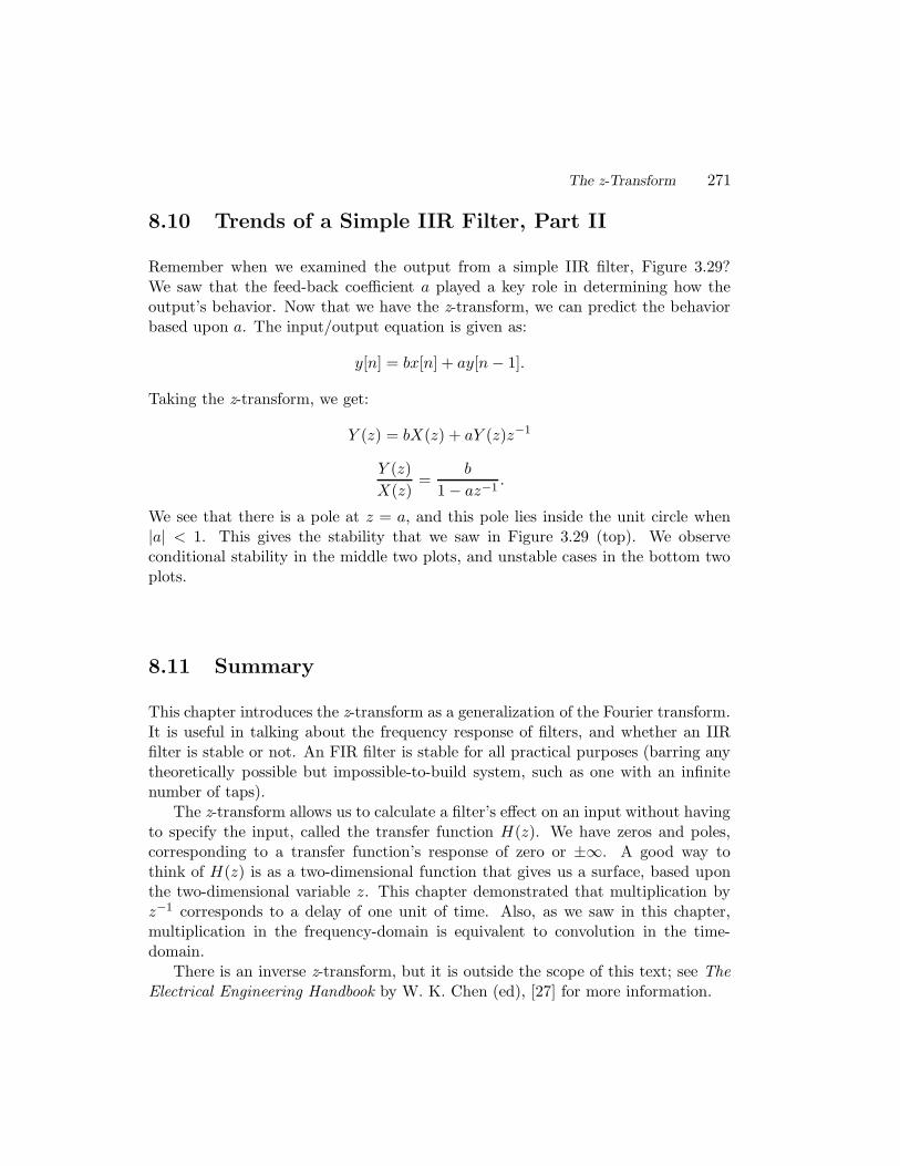
The z-Transform 271
8.10 Trends of a Simple IIR Filter, Part II
Remember when we examined the output from a simple IIR filter, Figure 3.29?We saw that the feed-back coefficient a played a key role in determining how theoutput’s behavior. Now that we have the z-transform, we can predict the behaviorbased upon a. The input/output equation is given as:
y[n] = bx[n] + ay[n− 1].
Taking the z-transform, we get:
Y (z) = bX(z) + aY (z)z−1
Y (z)
X(z)=
b
1 − az−1.
We see that there is a pole at z = a, and this pole lies inside the unit circle when|a| < 1. This gives the stability that we saw in Figure 3.29 (top). We observeconditional stability in the middle two plots, and unstable cases in the bottom twoplots.
8.11 Summary
This chapter introduces the z-transform as a generalization of the Fourier transform.It is useful in talking about the frequency response of filters, and whether an IIRfilter is stable or not. An FIR filter is stable for all practical purposes (barring anytheoretically possible but impossible-to-build system, such as one with an infinitenumber of taps).
The z-transform allows us to calculate a filter’s effect on an input without havingto specify the input, called the transfer function H(z). We have zeros and poles,corresponding to a transfer function’s response of zero or ±∞. A good way tothink of H(z) is as a two-dimensional function that gives us a surface, based uponthe two-dimensional variable z. This chapter demonstrated that multiplication byz−1 corresponds to a delay of one unit of time. Also, as we saw in this chapter,multiplication in the frequency-domain is equivalent to convolution in the time-domain.
There is an inverse z-transform, but it is outside the scope of this text; see TheElectrical Engineering Handbook by W. K. Chen (ed), [27] for more information.

272 DSP Using MATLAB and Wavelets
8.12 Review Questions
1. What is the z-transform of x = 3, 2, 4?
2. A FIR filter has the following filter coefficients: 1, −1. What is the frequencyresponse? Where are the zeros located? Use MATLAB to calculate the outputwith an input of cos(2π100t), sampled at fs = 200 samples/second.
3. A FIR filter has the following filter coefficients: 1, 1. What is the frequencyresponse? Where are the zeros located? Use MATLAB to calculate the outputwith an input of cos(2π100t), sampled at fs = 200 samples/second.
4. A filter has the following transfer function:
H(z) = (1 + 3z−1 − 4z−2)/(1 − z−1 − 6z−2).
a. Determine where the zeros and poles are.
b. Plot these (by hand) on the z-plane, with an x for a pole and an o fora zero. Is this filter stable?
c. Draw the filter in terms of multipliers, adders, and delay units.
5. What is the z-transform of the transfer function, H(z), for the following filters?
a. FIR filter with coefficients b[k] = -17, 29, 107, 62b. IIR filter with feed-forward coefficients b[k] = −17, 29, 107, 62 and feed-back coefficients a[k] = 4,−7,−26,−15
6. Where are the zeros and poles located for the following transfer functions?Are these filters stable?
a.
H(z) =1√2− 1√
2z−1
b.
H(z) =
1√2− 1√
2z−1
1 − z−1
c.H(z) = (1 + 4z−2)/(1 − 4z−1 + 3z−2)

The z-Transform 273
7. Suppose we have a filter with the following transfer function. What value forH(z) do we have when z = 2ejπ/6? What about when z = 2e−j2π6? Findthese analytically, and reduce the answer to a single complex value, then writea program to demonstrate this.
H(z) = 1 − z−1 + z−2


Chapter 9
The Wavelet Transform
The Discrete Wavelet Transform (DWT) is used in a variety of signal processingapplications, such as video compression [28], Internet communications compression[29], object recognition [30], and numerical analysis. It can efficiently representsome signals, especially ones that have localized changes. Consider the example ofrepresenting a unit impulse function with the Fourier transform, which needs aninfinite amount of terms because we are trying to represent a single quick changewith a sum of sinusoids. However, the wavelet transform can represent this short-term signal with only a few terms.
This transform came about from different fields, including mathematics, physics,and image processing. Essentially, people in different areas were doing the samething, but using different terminology. In the late 1980s, Stephane Mallat unifiedthe work into one topic [1].
This transform is discrete in time and scale. In other words, the DWT coefficientsmay have real (floating-point) values, but the time and scale values used to indexthese coefficients are integers. The wavelet transform is gaining popularity withthe recent JPEG-2000 standard, which incorporates multiresolution analysis. Thischapter explains how the wavelet transform works, and shows how the wavelet breaksa signal down into detail signals and an approximation.
We call an octave a level of resolution, where each octave can be envisioned as apair of FIR filters, at least for the one-dimensional case. One filter of the analysis(wavelet transform) pair is a lowpass filter (LPF), while the other is a highpass filter(HPF), Figure 9.1. Each filter has a down-sampler after it, to make the transformefficient. Figure 9.2 shows the synthesis (inverse wavelet transform) pair, consist-ing of an inverse lowpass filter (ILPF) and an inverse highpass filter (IHPF), eachpreceded by an up-sampler. A lowpass filter produces the average signal, while ahighpass filter produces the detail signal. For example, a simple lowpass filter may
275

276 DSP Using MATLAB and Wavelets
have coefficients 12 ,
12, producing outputs (x[n] + x[n− 1])/2, which is clearly the
average of two samples. A corresponding simple highpass filter would have coef-ficients 1
2 ,−12, producing outputs (x[n] − x[n − 1])/2, half the difference of the
samples. While the average signal would look much like the original, we need thedetails to make the reconstructed signal match the original. Multiresolution anal-ysis feeds the average signal into another set of filters, which produces the averageand detail signals at the next octave [1]. The detail signals are kept, but the higheroctave averages can be discarded, since they can be recomputed during the synthe-sis. Each octave’s outputs have only half the input’s amount of data (plus a fewcoefficients due to the filter). Thus, the wavelet representation is approximately thesame size as the original.
2
2
Input
X[n]
LPF
HPF
Figure 9.1: Analysis filters.
2
2
Output
Y[n]
ILPF
IHPF
Figure 9.2: Synthesis filters.
Using the discrete wavelet transform on images (or other 2D data) can be ac-complished with the dwt2 and idwt2 functions. Making your own 2D transformcan be accomplished in one of two ways; either by applying the low- and high-pass filters along the rows of the data, then applying each of these filters along thecolumns of the previous results, or by applying four matrix convolutions, one for eachlowpass/highpass, horizontal/vertical combination (i.e., low-horizontal low-vertical,low-horizontal high-vertical, etc.). Separability means that the 2D transform is sim-ply an application of the 1D DWT in the horizontal and vertical directions [31]. Thenonseparable 2D transform works a bit differently, since it computes the transformbased on a 2D sample of the input convolved with a matrix, but the results arethe same. Think of this as two ways of reaching the same answer; just as we cancombine two filters into one (section 8.2), we can combine horizontal and verticaloperations into a matrix multiplication.
The main difference between the 1D, 2D, and 3D DWT is that a pair of filters

The Wavelet Transform 277
operates on each channel for each dimension. Figures of these should not be takentoo literally, since there are more efficient ways to implement all three architectures[32].
This chapter examines how FIR filters can be used to perform the wavelet trans-form. First, we will look at the Haar transform, which was developed by AlfredHaar before the term “wavelet” was coined [33]. Later, we will examine the wavelettransform with the four-coefficient Daubechies wavelet [2]. The Daubechies waveletsare actually a generalization of the Haar transform, and sometimes the Haar trans-form is referred to as a 2-coefficient Daubechies wavelet. Daubechies actually has afamily of wavelets, using the pattern we see below, except with more coefficients.
9.1 The Two-Channel Filter Bank
To demonstrate a general transform, we use Figure 9.3 below. Here, an input signalfeeds to two channels, each with a pair of FIR filters. We call this structure atwo-channel filter bank.
Inputh1
h0
z[n]
w[n]
Outputg1
x[n] y[n]g0
Figure 9.3: A two-channel filter bank.
The left half of Figure 9.3 performs the forward transform, also called analysis,while the right half corresponds to the inverse transform, also called synthesis. Whenwe talk about a transform such as the Haar transform or the wavelet transform, werefer only to the analysis part, the left half of the figure. On the other hand, theinverse Haar transform takes place on the right half of the figure. Putting the forwardand inverse transforms together, we expect that the output of the two-channel filterbank (y[n]) is exactly the same as the input (x[n]), with the possible exception of atime delay, such as y[n] = x[n− k], where k = 1 for two coefficients.
The complementary filters of a filter bank divide the signal into subsignals oflow-frequency components and one of high-frequency components. This approach iscalled subband coding.
For the inverse transform, each of the filters’ outputs (w[n] and z[n]) goes toanother FIR filter, after which the two channels are recombined by addition to formy[n]. The idea is that w[n] and z[n] are a transformed version of x[n], and that y[n]is the signal after the inverse transform. We expect that y[n] is the same as x[n],assuming that we did not alter the signal along the way. If we wanted to perform

278 DSP Using MATLAB and Wavelets
lossy compression, for example, we might alter z[n] so that it can be stored moreefficiently. Of course, this would mean that y[n] would not be x[n] exactly, butrather it would be an approximation of x[n]. The discussion here assumes that wewant perfect reconstruction, that is, that y[n] will be an exact copy of x[n], thoughit may be a delayed version. To get perfect reconstruction, we have to choose ourfilter coefficients with care. Let’s use the following values:
h0 = a, b
h1 = b,−ag0 = b, ag0 = −a, b.
Let’s see what the signals w[n] and z[n] would be. This is the forward transform:
w[n] = ax[n] + bx[n− 1]
z[n] = bx[n] − ax[n− 1].
We will also need to know w[n−1] and z[n−1], which can be found by replacingn with n− 1:
w[n− 1] = ax[n− 1] + bx[n− 2]
z[n− 1] = bx[n− 1] − ax[n− 2].
Now we can talk about what y[n] is, after the inverse transform:
y[n] = bw[n] + aw[n− 1] − az[n] + bz[n− 1].
However, it is interesting to see how y[n] relates to the original signal, x[n]:
y[n] = b(ax[n] + bx[n− 1]) + a(ax[n− 1] + bx[n− 2])- a(bx[n] − ax[n− 1]) + b(bx[n− 1] − ax[n− 2])
y[n] = abx[n] + bbx[n− 1] + aax[n− 1] + abx[n− 2]- abx[n] + aax[n− 1] + bbx[n− 1] - abx[n− 2].
Repeating the previous equation, but eliminating the parts that cancel:
y[n] = bbx[n− 1] + aax[n− 1]+ aax[n− 1] + bbx[n− 1]
The Wavelet Transform 279
y[n] = (2aa+ 2bb)x[n− 1].
The Haar transform is a very simple wavelet transform. If we carefully chooseour coefficients a and b above, we will have the Haar transform. If 2aa + 2bb = 1,then y[n] = x[n−1], meaning that the output is the same as the input, only delayedby 1. We can handle the coefficients a and b in one of two ways. Either we canmake them both 1, which makes the filters easier to implement, and then rememberto divide all y[n] values by (2 × 12 + 2 × 12) = 4, or we can choose our a and bvalues to make sure that (aa + bb) = 1. If we force aa = 1/2, and bb = 1/2, thena = b = 1/
√2. These values correspond to the Haar transform. The reason we
want (aa + bb) = 1 and not 2(aa + bb) = 1 has to do with the down/up-samplers,discussed later in this chapter.
9.2 Quadrature Mirror Filters and ConjugateQuadrature Filters
Sometimes two-channel filter banks are referred to as subband coders. Here, wewill use the terms interchangeably, though subband coders may have more than twochannels. You may also see a two-channel filter bank called a quadrature mirror filter(QMF), or a conjugate quadrature filter (CQF), though “two-channel filter bank”is the most general of these three terms. The QMF and CQF both put conditionson the filter coefficients to cancel aliasing terms and get perfect reconstruction. Inother words, a quadrature mirror filter and a conjugate quadrature filter are bothtypes of two-channel filter banks, with the same structure. The only differencesbetween a QMF, CQF, or another two-channel filter bank are the filter coefficients.
We specify the coefficients in terms of one of the analysis filters, and we will labelthese coefficients h0. The other filter coefficients (h1, g0, g1) are typically obtainedfrom h0. After all, we cannot just use any values we want for the filter coefficientsor the end result will not match our original signal.
Essentially, a quadrature mirror filter specifies that h1 uses the same filter co-efficients as h0, but negates every other value. The reconstruction filter g0 is thesame as h0, and the filter coefficients g1 = −h1, meaning that we copy h1 to g1 andnegate all of g1’s values. See Figure 9.4 for an example using two coefficients. Aninteresting note about the QMF is that this does not work in general. Practicallyspeaking, the QMF has only two coefficients (unless one uses IIR filters).
The conjugate quadrature filter specifies h1 as a reversed version of h0, with

280 DSP Using MATLAB and Wavelets
Inputa, −b
a, b
z[n]
w[n]
Output−a, b
a, bx[n] y[n]
Figure 9.4: A quadrature mirror filter for the Haar transform.
every other value negated [34]. If h0 = [a, b, c, d], then h1 will be [d,−c, b,−a] 1.For reconstruction, g0 and g1 are reversed versions of h0 and h1, respectively. Usingthe h0 values from above, we get g0 = [d, c, b, a], and g1 = [−a, b,−c, d]. Figure 9.5shows what this looks like for two coefficients.
Inputb, −a
a, b
z[n]
w[n]
Output−a, b
b, ax[n] y[n]
Figure 9.5: A conjugate quadrature filter for the Haar transform.
For two coefficients that are the same (a = b in the figures), the QMF and theCQF have identical filter coefficients. The CQF is actually an improvement of theQMF, in the sense that it works for larger filters (assuming an even number of filtercoefficients). Notice that both Figures 9.4 and 9.5 specify the Haar transform whena = b. We will use this transform often, since it has only two coefficients, but it isan example of a wavelet.
Though there are four filters, the name (“quadrature”) actually comes from thefact that the frequency responses of the lowpass and highpass filters are symmetricaround the “quadrature” point π/2. Consider the spectrum of a filter’s response:for real signals, we show only the first half, frequencies from 0 to π. If we dividethis into an ideal lowpass and highpass section, we divide it halfway again, i.e., atpoint π/2. The “mirror” term comes from the highpass filter’s frequency magnituderesponse being a mirror image of the lowpass filter’s frequency magnitude.
9.3 How the Haar Transform Is a 45-Degree Rotation
A basis is a projection onto a coordinate axis. If we have a point on a graph, wecan talk of its distance from the origin, another point used for reference. But this
1MATLAB uses h1 = [−d, c,−b, a].

The Wavelet Transform 281
only narrows it down to a circle, so we need more information: the angle betweenthe vector made by the origin to the point of interest, and another line for reference(i.e., the x-axis). For a point in 2D space, these polar coordinates are sufficientinformation to unambiguously locate the point with respect to the origin. But weoften use the Cartesian basis 1, 0 and 0, 1 to represent this point, which tellsabout the point in terms of a unit vector along the x-axis and another unit vectoralong the y-axis (they are normalized). We know that the y-axis intersects thex-axis at the origin, and that there is a 90-degree angle between them (they areorthogonal). Though, generally speaking, we could use a different set of axes (i.e.,a different basis).
The Haar basis is 1/√
2, 1/√
2 and 1/√
2, −1/√
2 , instead of the normalCartesian basis. This section answers the question of what the points look like in theHaar-domain instead of the Cartesian-domain. What we will see is that the pointshave the same relationship to one another, but the coordinate system moves by arotation of 45 degrees.
First, consider the points (x1, y1), (x2, y2), etc. as the array x1, y1, x2, y2, etc..The Cartesian system simply isolates the x’s and y’s, as in:
[1 0] 0 0[0 1] 0 00 0 [1 0]0 0 [0 1]
x1
y1
x2
y2
.
Whereas the Haar system does the following:
1√2
[1 1] 0 0[1 − 1] 0 0
0 0 [1 1]0 0 [1 − 1]
x1
y1
x2
y2
.
For example, the Cartesian coordinates (1, 10) would be mapped to(
1+10√2, 1−10√
2
)
,
or(
11√2, −9√
2
)
in the Haar-domain.
9.3.1 How The Haar Transform Affects a Point’s Radius
Consider these numbers to be vectors (i.e., in polar coordinates). The magnitudeand angle can be found with a little geometry. In fact, the magnitude can be foundusing Pythagoras’ theorem. The magnitude of the Cartesian coordinates (1, 10) is

282 DSP Using MATLAB and Wavelets
√12 + 102 =
√101. The magnitude of the Haar coordinates
(
11√2, −9√
2
)
is
√
(
11√2
)2
+
(−9√2
)2
=
√
121
2+
81
2=
√
202
2=
√101.
This example shows that the magnitudes are the same. In other words, when weconsider the point (1, 10) as a distance from the origin and a rotation from thepositive x-axis, the Haar transform does not affect the distance. We can show thatthis is the case for ANY arbitrary point by replacing (1, 10) above with (x, y). In
the Haar-domain, we would have points(
x+y√2, x−y√
2
)
. Now, considering these points
as polar coordinates, we see that the magnitude of the Cartesian coordinates is√
x2 + y2. The magnitude of the Haar coordinates is
√
(
x+ y√2
)2
+
(
x− y√2
)2
=
√
(
x2 + 2xy + y2
2
)
+
(
x2 − 2xy + y2
2
)
=
√
2x2 + 2y2
2=√
x2 + y2.
Therefore, the Haar transform does not affect the distance of a point from the origin.It does, however, affect the angle of the point in relation to the x-axis.
9.3.2 How The Haar Transform Affects a Point’s Angle
To see how the angle changes for the Haar transform, we will start again with the
point (1, 10), which we know becomes(
11√2, −9√
2
)
in the Haar-domain. What are the
angles that these points make with respect to their x-axes? The formula for findingthe angles (labeled theta) is given below. Note that atan finds the arctangent.
if (x > 0)
theta = atan (y/x)
elseif (x < 0)
if (y < 0)
theta = atan (y/x) - pi
else
theta = atan (y/x) + pi
end
else
% The vector lies on the y-axis.

The Wavelet Transform 283
theta = sign(y)*(pi/2)
end
The angle made by the Cartesian coordinates (1, 10) is 84.29. The angle madeby the same coordinates after the Haar transform is tan−1
(−911
)
= −39.29.Looking at the relationship between the two in general, the AngleCartesian =
tan−1( y
x
)
, while the AngleHaar = tan−1(
(x−y)/√
2
(x+y)/√
2
)
= tan−1(
x−yx+y
)
.
The formula above is rather cumbersome to deal with, due to the ambiguousnature of the arctan function, and because of a potential divide-by-zero problemwhen x = 0. For the first consideration, this becomes a little easier when wereplace x and y with their polar coordinate equivalents. That is, we will replace xand y with r cos(θ1) and r sin(θ1), respectively. The Haar-domain values are thenr(cos(θ1) + sin(θ1))/
√2 and r(cos(θ1) − sin(θ1))/
√2, respectively. Finding the new
angle (the Haar-domain angle, θ2), we plug the Haar-domain values from above intothe equation θ = tan−1( y
x) to find:
θ2 = tan−1
(
r(cos(θ1) − sin(θ1))/√
2
r(cos(θ1) + sin(θ1))/√
2
)
.
An interesting thing to notice is that the term r/√
2 cancels itself out, meaning thatthe radii of the polar values do not matter. In other words, the value for θ2 dependssolely on θ1. This should be expected, since we already know from section 9.3.1 thatthe two radii are equal. So the equation for θ2 simplifies to:
θ2 = tan−1
(
cos(θ1) − sin(θ1)
cos(θ1) + sin(θ1)
)
.
We can divide by cos(θ1), giving us:
θ2 = tan−1
cos(θ1)cos(θ1) −
sin(θ1)cos(θ1)
cos(θ1)cos(θ1) + sin(θ1)
cos(θ1)
θ2 = tan−1
1 − sin(θ1)cos(θ1)
1 + sin(θ1)cos(θ1)
.
We then replace sin(θ1)cos(θ1) with tan(θ1):
θ2 = tan−1
(
1 − tan(θ1)
1 + tan(θ1)
)
.

284 DSP Using MATLAB and Wavelets
Since tan(π/4) = 1, we will replace the 1 in the numerator. Also in the denominator,tan(θ1) = 1 × tan(θ1) = tan(π/4)tan(θ1). This gives us:
θ2 = tan−1
(
tan(π/4) − tan(θ1)
1 + tan(π/4)tan(θ1)
)
.
Now comes the point of all this manipulation. There is a trigonometric identity2
that says:
tan(α− β) =tan(α) − tan(β)
1 + tan(α)tan(β).
It is no coincidence that the right side of the above identity looks a lot like part ofour expression for θ2. Once we use this identity, it simplifies our equation:
θ2 = tan−1(tan(π/4 − θ1))
θ2 = π/4 − θ1.
This says what we expect it to; that the Haar transform is a rotation by π/4 radians,or 45 degrees.
9.4 Daubechies Four-Coefficient Wavelet
Let’s also consider the case of four coefficients in a conjugate quadrature filter.Figure 9.6 shows a structure similar to Figure 9.5, except that its FIR filters havefour taps (use four coefficients).
Input
z[n]
w[n]
Output
x[n] y[n]a, b, c, d
d, −c, b, −a −a, b, −c, d
d, c, b, a
Figure 9.6: A two-channel filter bank with four coefficients.
The expressions for w[n] and z[n] can be found in a similar manner as in section9.1:
w[n] = ax[n] + bx[n− 1] + cx[n− 2] + dx[n− 3]
z[n] = dx[n] − cx[n− 1] + bx[n− 2] − ax[n− 3].
2Thanks to Mr. Srikanth Tirupathi for pointing this out.

The Wavelet Transform 285
We will also need w[n− 1], w[n− 2], and so forth, so it is helpful to define thesefor an integer k:
w[n− k] = ax[n− k] + bx[n− k − 1] + cx[n− k − 2] + dx[n− k − 3]z[n− k] = dx[n− k] − cx[n− k − 1] + bx[n− k − 2] − ax[n− k − 3].
Now we can put this all together, and express y[n] in terms of x[n] only:
y[n] = dw[n] + cw[n− 1] + bw[n− 2] + aw[n− 3]− az[n] + bz[n− 1] − cz[n− 2] + dz[n− 3]
y[n] = d(ax[n] + bx[n− 1] + cx[n− 2] + dx[n− 3])+ c(ax[n− 1] + bx[n− 2] + cx[n− 3] + dx[n− 4])+ b(ax[n− 2] + bx[n− 3] + cx[n− 4] + dx[n− 5])+ a(ax[n− 3] + bx[n− 4] + cx[n− 5] + dx[n− 6])− a(dx[n] − cx[n− 1] + bx[n− 2] − ax[n− 3])
+ b(dx[n− 1] − cx[n− 2] + bx[n− 3] − ax[n− 4])− c(dx[n− 2] − cx[n− 3] + bx[n− 4] − ax[n− 5])+ d(dx[n− 3] − cx[n− 4] + bx[n− 5] − ax[n− 6]).
Multiplying through:
y[n] = adx[n] + bdx[n− 1] + cdx[n− 2] + ddx[n− 3]+ acx[n− 1] + bcx[n− 2] + ccx[n− 3] + cdx[n− 4]+ abx[n− 2] + bbx[n− 3] + bcx[n− 4] + bdx[n− 5]+ aax[n− 3] + abx[n− 4] + acx[n− 5] + adx[n− 6]− adx[n] + acx[n− 1] − abx[n− 2] + aax[n− 3]
+ bdx[n− 1] − bcx[n− 2] + bbx[n− 3] − abx[n− 4]− cdx[n− 2] + ccx[n− 3] − bcx[n− 4] + acx[n− 5]+ ddx[n− 3] − cdx[n− 4] + bdx[n− 5] − adx[n− 6].
Now we rewrite this equation to line up the x[n− k] values properly:

286 DSP Using MATLAB and Wavelets
y[n] =adx[n] + bdx[n− 1] + cdx[n− 2] + ddx[n− 3]
+ acx[n− 1] + bcx[n− 2] + ccx[n− 3] + cdx[n− 4]+ abx[n− 2] + bbx[n− 3] + bcx[n− 4]
+ bdx[n− 5] + aax[n− 3] + abx[n− 4]+ acx[n− 5] + adx[n− 6]−adx[n] + acx[n− 1] − abx[n− 2] + aax[n− 3]
+ bdx[n− 1] − bcx[n− 2] + bbx[n− 3] − abx[n− 4]− cdx[n− 2] + ccx[n− 3] − bcx[n− 4]
+ acx[n− 5] + ddx[n− 3] − cdx[n− 4]+ bdx[n− 5] − adx[n− 6].
Repeating the above equation, only eliminating the parts that cancel:
y[n] = bdx[n− 1] + ddx[n− 3]+ acx[n− 1] + ccx[n− 3]
+ bbx[n− 3] + bdx[n− 5]+ aax[n− 3] + acx[n− 5]
+ acx[n− 1] + aax[n− 3]+ bdx[n− 1] + bbx[n− 3]
+ ccx[n− 3] + acx[n− 5]+ ddx[n− 3] + bdx[n− 5].
The terms x[n − 1] and x[n − 5] are pesky, since we want each output of y[n]to depend upon only one input of x[n]. But if ac happens to equal −bd, then theseterms will cancel each other out. Therefore, we will make this a requirement. Ifac+bd = 0, then the x[n−1] and x[n−5] terms are eliminated, and we are left with:
y[n] = 2(aa+ bb+ cc+ dd)x[n− 3]
or that y[n] is a delayed version of x[n], multiplied by a constant. Of course, wecould have a second requirement that this constant be 1. The Daubechies coeffi-cients satisfy both of these criteria: (These are the lowpass coefficients from db2,obtained from MATLAB)a = −0.1294b = 0.2241c = 0.8365d = 0.4830
ac = −0.1083

The Wavelet Transform 287
bd = 0.1083.
Errors due to precision come about when using wavelets. The coefficients above areactually an approximation of the following Daubechies coefficients (obtained from[3]):
a =1 −
√3
4√
2, b =
3 −√
3
4√
2, c =
3 +√
3
4√
2, d =
1 +√
3
4√
2.
Note that the reference gives these as the highpass filter coefficients, which meansthat the b and d values above were negated. So,
ac =−2
√3
32, bd =
2√
3
32.
Therefore:ac = −bd.
Using these coefficients, we see that:
a2 =4 − 2
√3
32, b2 =
12 − 6√
3
32, c2 =
12 + 6√
3
32, d2 =
4 + 2√
3
32.
Finding the sum aa+ bb+ cc+ dd leads to:
a2 + b2 + c2 + d2 =4 − 2
√3 + 12 − 6
√3 + 12 + 6
√3 + 4 + 2
√3
32
a2 + b2 + c2 + d2 =4 + 12 + 12 + 4
32
a2 + b2 + c2 + d2 = 1.
This is what we should expect—that the values for a, b, c, and d are carefully chosenso that the output y[n] is just a delayed version of the input x[n]. But above wefound that y[n] = 2(aa + bb + cc + dd)x[n − 3], so these coefficients mean thaty[n] = 2x[n− 3]. Why is the 2 there? The answer for this lies in the down-samplingoperation. We have not yet looked at the effect of the down-sampling operation,but it gives us the same outputs, only at 1/2 the scale. That is, if we use the aboveDaubechies coefficients, but with down-samplers and up-samplers in place, then weget y[n] = x[n− 3]. This is why aa+ bb+ cc+ dd = 1, instead of 1/2. This is shownin section 9.5.

288 DSP Using MATLAB and Wavelets
9.5 Down-Sampling and Up-Sampling
The down-sampling operation is easy enough to envision: only the even indexedvalues are kept. It squeezes the signal to half of its size. The inverse operation,up-sampling, stretches the signal back out, usually by inserting a 0 between eachtwo successive samples. The effect of a down-sampler followed by an up-sampler isthat every other value will be 0.
In this text, we show the down-sampler as the arrow followed by the number 2,as in the top left corner of Figure 9.7, and the up-sampler as in the top right cornerof the same figure. Alternatively, some texts use the two symbols along the bottomof this figure [35], as in two inputs enter but only one leaves for the down-sampler,and one input enters but two exit the up-sampler.
2 2
12 21
Figure 9.7: Different ways to indicate down-samplers and up-samplers.
9.5.1 Example Using Down/Up-Samplers
Intuitively, using up- and down-samplers may seem like it cannot work. How can wethrow out half of our calculations after filtering without losing information? Thissection gives a brief example of how this process works.
Figure 9.8 shows an example of a two-channel filter bank with down-samplersfollowed by up-samplers. The filters are very simple, in fact, these filters would beimplemented as in Figure 8.2, which reduces down to Figure 8.3.
1, 02
2 2
2
Input1, 0
y[n]x[n]
Output
0, 1
0, 1
Figure 9.8: A simple filter bank demonstrating down/up-sampling.
Since the filter with coefficients 1, 0 allows the input to pass through to theoutput, we will replace it with a simple line. Likewise, we can replace the filter with

The Wavelet Transform 289
coefficients of 0, 1 with a delay unit. With these modifications in place, we havethe revised filter of Figure 9.9.
D
2
2 2
2
Input
x[n] y[n]
Output
D
Figure 9.9: A simple filter bank demonstrating down/up-sampling, reduced.
Now we are ready to trace an input through to the output, with the values x[0],x[1], x[2], x[3], x[4], x[5], etc. Keep in mind that these inputs are listed in orderfrom left to right, so that x[0] enters the filter bank first, followed by x[1], and soforth.
y[n]
2
2 2
2D
D0, x[0], 0, x[2], 0, x[4], 0, ...
0, 0, x[1], 0, x[3], 0, x[5], ...
x[0], x[1], x[2], x[3], x[4], x[5], ...
x[0], x[2], x[4], ...
x[0], 0, x[2], 0, x[4], 0, ...
0, x[0], x[1], x[2], x[3], x[4], x[5], ...
0, x[1], x[3], x[5], ...
Figure 9.10: Tracing input to output of a simple filter bank.
Looking at the top channel of Figure 9.10, we see the input values go to thedown-sampler, whose output is x[0], x[2], x[4], etc., the even values of x. Theforward transform ends here for this channel, but we will see what this channelcontributes to the output. The up-sampler inserts zeros between values, to generatethe sequence x[0], 0, x[2], 0, x[4], 0, etc. Next comes the delay unit, which meansthat every input to it will appear at the output one time step later. We note thisas a zero for its first output, followed by the signal that reaches it. The reason forthe delay unit should be apparent when we consider the bottom channel. Thus, thetop channel contributes a signal of 0, x[0], 0, x[2], 0, x[4], 0, etc., the even values ofx with zeros between the values.

290 DSP Using MATLAB and Wavelets
Now we turn our attention to the bottom channel of Figure 9.10. The delay unitshifts our inputs over one unit, so its first output is zero, followed by x[0], x[1], x[2],etc. When this signal reaches the down-sampler, it has the effect of removing everyother value. Since 0 is the first input, it passes through, while x[0] is discarded.Thus, the down-sampler’s output is 0, x[1], x[3], x[5], etc. At the end of the forwardtransform for the bottom channel, we see that we have the odd values for x. Thesynthesis side of the QMF for the bottom channel simply up-samples the signal.This results in the pattern 0, 0, x[1], 0, x[3], 0, x[5], etc.
Combining the top channel with the bottom channel with addition results in0 + 0, x[0] + 0, 0 + x[1], x[2] + 0, 0 + x[3], x[4] + 0, 0 + x[5], etc.
This demonstration shows that performing down and up-sampling on the chan-nels of a QMF is not as crazy as it sounds. In effect, the QMF of Figure 9.8 breaksthe input into its even values and its odd values, then adds them back together.This results in an output that matches the input, except for a delay.
9.5.2 Down-Sampling and Up-Sampling with 2 Coefficients
With wavelets, the filter bank structure will include down-samplers and up-samplersin the following configuration, Figure 9.11. In each channel, the signal undergoesseveral changes. To keep them distinct, they are each labeled. In the upper channel,we have z[n], which is the output from the first or “analyzing” FIR filter, then zd[n]corresponds to z[n] after it has been down-sampled, then zu[n] represents the signalafter up-sampling, and finally zf [n] gives us the final values for that channel.
2
2 2
2w [n]d
z [n]d
w [n]u
z [n]u z [n]f
w [n]f
Inputb, −a
y[n]x[n]
Output
a, b b, a
−a, b
w[n]
z[n]
Figure 9.11: A two-channel filter bank with down/up-samplers.
Signals w[n] and z[n] are just as they were in section 9.1:
w[n] = ax[n] + bx[n− 1]
z[n] = bx[n] − ax[n− 1].
Signals w[n− 1] and z[n− 1], are again found by replacing n above with n− 1:
w[n− 1] = ax[n− 1] + bx[n− 2]

The Wavelet Transform 291
z[n− 1] = bx[n− 1] − ax[n− 2].
Looking at wd[n] and zd[n], we have to be a bit careful. We make the statementsbelow for the even values of n. When n is odd, there is no value for wd[n] or zd[n]!
wd[n] = w[n], n is even
zd[n] = z[n], n is even
Signals wu[n] and zu[n] must be treated with equal caution.
wu[n] = wd[n] = w[n], n is even
wu[n] = 0, n is odd
zu[n] = zd[n] = z[n], n is even
zu[n] = 0, n is odd
We have values for wu[n] and zu[n] for even and odd values of n. So when usingthese signals for n and n − 1, one of the indices must be even, while the other isodd. The final signals of each channel are:
wf [n] = bwu[n] + awu[n− 1]
wf [n] = bw[n] + 0, n is even
wf [n] = 0 + aw[n− 1], n is odd
zf [n] = −azu[n] + bzu[n− 1]
zf [n] = −az[n] + 0, n is even
zf [n] = 0 + bz[n− 1], n is odd.
When we combine wf [n] and zf [n] to form y[n], we still have to concern ourselveswith whether the index is even or odd.
y[n] = bw[n] − az[n], n is even
y[n] = aw[n− 1] + bz[n− 1], n is odd
These expressions can be expanded, to put the output y[n] in terms of the originalinput x[n].

292 DSP Using MATLAB and Wavelets
y[n] = b(ax[n] + bx[n− 1]) − a(bx[n] − ax[n− 1]), n is even
y[n] = a(ax[n− 1] + bx[n− 2]) + b(bx[n− 1] − ax[n− 2]), n is odd
Simplifying:
y[n] = abx[n] + bbx[n− 1] − abx[n] + aax[n− 1], n is even
y[n] = aax[n− 1] + abx[n− 2] + bbx[n− 1] − abx[n− 2], n is odd.
Eliminating terms that cancel each other out, and simplifying further:
y[n] = (aa+ bb)x[n− 1], n is even
y[n] = (aa+ bb)x[n− 1], n is odd.
This last step is important, where we see that y[n] is in terms of x[n− 1] regardlessof whether n is even or odd. If we compare this result to the result of section 9.1,also dealing with Haar coefficients, we see that the difference is a factor of 2. TheHaar coefficients are usually given as 1/
√2, 1/
√2, so that (aa+ bb) = 1.
9.5.3 Down-Sampling and Up-Sampling with Daubechies 4
This is why the coefficients from the Daubechies four-coefficient wavelet, when usedwithout the down-sampler and up-sampler, ended up with y[n] = 2x[n− 3]. If thedown-samplers and up-samplers are included, then the 2 term drops out. This isshown later. First, we will start, as usual, with Figure 9.12, an updated filter bankfor four coefficients in each filter.
2
2 2
2w [n]d
z [n]d
w [n]u
z [n]u z [n]f
w [n]f
Input
y[n]x[n]
Output
w[n]
z[n]d, −c, b, −a
a, b, c, d
−a, b, −c, d
d, c, b, a
Figure 9.12: A filter bank with four taps per filter.
Signals w[n] and z[n] are just as they were earlier:

The Wavelet Transform 293
w[n] = ax[n] + bx[n− 1] + cx[n− 2] + dx[n− 3]
z[n] = dx[n] − cx[n− 1] + bx[n− 2] − ax[n− 3].
Signals w[n− k] and z[n− k], are again found by replacing n with n− k:
w[n− k] = ax[n− k] + bx[n− k − 1] + cx[n− k − 2] + dx[n− k − 3]
z[n− k] = dx[n− k] − cx[n− k − 1] + bx[n− k − 2] − ax[n− k − 3].
Looking at wd[n] and zd[n], we again have to be careful about whether n is even orodd. When n is odd, there is no value for wd[n] or zd[n]!
wd[n] = w[n], n is even
zd[n] = z[n], n is even
Signals wu[n] and zu[n] must be treated with equal caution:
wu[n] = wd[n] = w[n], n is even
wu[n] = 0, n is odd
zu[n] = zd[n] = z[n], n is even
zu[n] = 0, n is odd.
We have values for wu[n] and zu[n] for even and odd values of n. So when usingthese signals for n and n − 1, one of indices must be even, while the other is odd.Likewise, if n is even, then so is n−2, n−4, etc. The final signals of each channel are:
wf [n] = dwu[n] + cwu[n− 1] + bwu[n− 2] + awu[n− 3]
wf [n] = dw[n] + 0 + bw[n− 2] + 0, n is even
wf [n] = 0 + cw[n− 1] + 0 + aw[n− 3], n is odd
zf [n] = −azu[n] + bzu[n− 1] − czu[n− 2] + dzu[n− 3]
zf [n] = −az[n] + 0 − cz[n− 2] + 0, n is even
zf [n] = 0 + bz[n− 1] + 0 + dz[n− 3], n is odd.

294 DSP Using MATLAB and Wavelets
Keeping track of whether index n is even or odd, we can find y[n] = wf [n] + zf [n]:
y[n] = dw[n] + bw[n− 2] − az[n] − cz[n− 2], n is even
y[n] = cw[n− 1] + aw[n− 3] + bz[n− 1] + dz[n− 3], n is odd.
These expressions can be expanded, to put the output y[n] in terms of the originalinput x[n]:
y[n] = d(ax[n] + bx[n− 1] + cx[n− 2] + dx[n− 3])
+b(ax[n− 2] + bx[n− 3] + cx[n− 4] + dx[n− 5])
−a(dx[n] − cx[n− 1] + bx[n− 2] − ax[n− 3])
−c(dx[n− 2] − cx[n− 3] + bx[n− 4] − ax[n− 5]), n is even
y[n] = c(ax[n− 1] + bx[n− 2] + cx[n− 3] + dx[n− 4])
+a(ax[n− 3] + bx[n− 4] + cx[n− 5] + dx[n− 6])
+b(dx[n− 1] − cx[n− 2] + bx[n− 3] − ax[n− 4])
+d(dx[n− 3] − cx[n− 4] + bx[n− 5] − ax[n− 6]), n is odd.
Simplifying:
y[n] = adx[n] + bdx[n− 1] + cdx[n− 2] + ddx[n− 3]
+abx[n− 2] + bbx[n− 3] + bcx[n− 4] + bdx[n− 5]
−adx[n] + acx[n− 1] − abx[n− 2] + aax[n− 3]
−cdx[n− 2] + ccx[n− 3] − bcx[n− 4] + acx[n− 5], n is even
y[n] = acx[n− 1] + bcx[n− 2] + ccx[n− 3] + cdx[n− 4]
+aax[n− 3] + abx[n− 4] + acx[n− 5] + adx[n− 6]
+bdx[n− 1] − bcx[n− 2] + bbx[n− 3] − abx[n− 4]
+ddx[n− 3] − cdx[n− 4] + bdx[n− 5] − adx[n− 6], n is odd.
Eliminating terms that cancel each other out, and simplifying further:

The Wavelet Transform 295
y[n] = acx[n− 1] + bdx[n− 1]
+aax[n− 3] + bbx[n− 3] + ccx[n− 3] + ddx[n− 3]
+acx[n− 5] + bdx[n− 5], n is even
y[n] = acx[n− 1] + bdx[n− 1]
+aax[n− 3] + bbx[n− 3] + ccx[n− 3] + ddx[n− 3]
+acx[n− 5] + bdx[n− 5], n is odd.
In this final step, we notice two things. First, the expressions are the same regardlessof whether n is even or odd, so now we can represent it as a single statement:
y[n] = aax[n− 3] + bbx[n− 3] + ccx[n− 3] + ddx[n− 3]
+acx[n− 1] + bdx[n− 1] + acx[n− 5] + bdx[n− 5].
Second, we see that we have x[n− 1] and x[n− 5] terms again, but that these canbe eliminated if we require ac = −bd. Assuming this is the case, we have our finalexpression for y[n]:
y[n] = (aa+ bb+ cc+ dd)x[n− 3].
If we compare this result to the earlier case (without down-sampling) we see that thedifference is a factor of 2. This explains why the sum of the squares of the Daubechiescoefficients, (aa+ bb+ cc+ dd) equals 1. When that is the case, y[n] = x[n− 3], ory[n] is simply a copy of x[n], delayed by 3 time units.
9.6 Breaking a Signal Into Waves
Just as the discrete Fourier transform breaks a signal into sinusoids, the discretewavelet transform generates “little waves” from a signal. These waves can then beadded together to reform the signal. Figure 9.13 shows the wavelet analysis forthree octaves on the left, with the standard synthesis (reconstruction) on the right.“LPF” stands for lowpass filter, while “HPF” means highpass filter. The “ILPF”and “IHPF” are the inverse low- and highpass filters, respectively. Although thedown-sampling and up-sampling operations are not explicitly shown, they can beincluded in the filters without loss of generality. On the right, there is an impliedaddition when two lines meet.
Figure 9.14 shows an alternate way to do the reconstruction. While not asefficient as Figure 9.13, it serves to demonstrate the contribution of each channel.

296 DSP Using MATLAB and Wavelets
HPF
LPF
HPF
LPF
HPF
ILPF
IHPF ILPF
IHPF ILPF
IHPF
LPF
Figure 9.13: Wavelet analysis and reconstruction.
In the end, we have four signals: three detail signals, and one level-3 approximation.
HPF
LPF
HPF
LPF
HPF
ILPF
IHPF ILPF
IHPF ILPF
IHPF
ILPF
ILPF
ILPF
LPF
Figure 9.14: Alternate wavelet reconstruction.
This section rests on the argument that we can rearrange the operations in thereconstruction, i.e., that we can perform the up-sampling and filtering first, andthen do the addition. We know that the ILPF and IHPF are made with FIR filtersthat have constant filter coefficients and are, therefore, linear. Thus, we know thatit does not matter whether we add two signals together and filter their sum, or filterthe two then add the results together. But what if we have down and up-samplers inthe analysis and reconstruction? Specifically for our purposes here, does it matter ifwe up-sample two signals first, then add them together, as opposed to adding themtogether, then up-sampling their sum? For simplicity, let’s call the two signals xand y, and consider only the first four samples of each. If we add these signals, weget:
[x0 + y0, x1 + y1, x2 + y2, x3 + y3].
Next, we up-sample this result to get:
[x0 + y0, 0, x1 + y1, 0, x2 + y2, 0, x3 + y3, 0].

The Wavelet Transform 297
Now consider what happens if we up-sample each signal first, then add them. Afterup-sampling them, we have:
[x0, 0, x1, 0, x2, 0, x3, 0]
and[y0, 0, y1, 0, y2, 0, y3, 0].
If we add them together now, we get:
[x0 + y0, 0, x1 + y1, 0, x2 + y2, 0, x3 + y3, 0].
We see that this exactly matches the result from adding first, then up-sampling.Also, the above argument works for arbitrary lengths of x and y. Also note that wecan recursively apply this reasoning and conclude that the reconstructions shown inFigures 9.13 and 9.14 are equivalent.
In Figure 9.15, we see the four signals that, when added together, reform theimpulse function. Figure 9.16 shows another four waves that reform the impulsefunction when added. The difference between these two is the wavelet used; inFigure 9.15, we used the Haar wavelet, while we used the Daubechies-2 (db2) waveletin Figure 9.16. Both of these figures show how the DWT represents the input signalas shifted and scaled versions of the wavelet and scaling functions. Since we use animpulse function, the wavelet function appears in the “High wave” signals, while thescaling function appears in the “Low wave” signals (or the “Low-Low-Low wave”signals in the case of these two figures).
It may be difficult to see from the figure that these four signals do cancel eachother out. To make this easier, Table 9.1 shows the actual values correspondingto the plots shown in Figure 9.15. The impulse signal used has 100 values, all ofwhich are zero except for a value of 1 at offset 50. Rather than give all values inthe table, we leave out the zeros and just show the values in the range 49 to 56.As the reader can verify, all columns of this table add to zero except for the secondcolumn. Belonging to the offset 50, the sum of this column is 1 just as the originalimpulse signal has a 1 at offset 50.
Figure 9.17 shows the input (impulse function) versus the output. As expected,the output signal exactly matches the input signal.
A more typical example is seen in Figure 9.18, a signal chosen because it clearlyshows the Haar wavelets in the first three subplots. (The example array 9, −2,5, −2, 7, −6, 4, −4 was used here.) The top plot shows four repetitions of theHaar wavelet, each of a different scale. The second subplot shows two repetitions,but these are twice as long as the ones above it. In the third subplot, one Haar

298 DSP Using MATLAB and Wavelets
10 20 30 40 50 60 70 80 90 100−0.5
0
0.5High wave (level 1 detail)
10 20 30 40 50 60 70 80 90 100−0.5
0
0.5Low−High wave (level 2 detail)
10 20 30 40 50 60 70 80 90 100−0.2
0
0.2Low−Low−High wave (level 3 detail)
10 20 30 40 50 60 70 80 90 100−0.2
0
0.2Low−Low−Low wave (level 3 approximation)
Figure 9.15: Impulse function analyzed with Haar.
Table 9.1: Impulse function analyzed with Haar.
-0.5000 0.5000 0 0 0 0 0 0
0.2500 0.2500 -0.2500 -0.2500 0 0 0 0
0.1250 0.1250 0.1250 0.1250 -0.1250 -0.1250 -0.1250 -0.1250
0.1250 0.1250 0.1250 0.1250 0.1250 0.1250 0.1250 0.1250

The Wavelet Transform 299
10 20 30 40 50 60 70 80 90 100−0.5
0
0.5High wave (level 1 detail)
10 20 30 40 50 60 70 80 90 100−0.5
0
0.5Low−High wave (level 2 detail)
10 20 30 40 50 60 70 80 90 100−0.5
0
0.5Low−Low−High wave (level 3 detail)
10 20 30 40 50 60 70 80 90 100−0.5
0
0.5Low−Low−Low wave (level 3 approximation)
Figure 9.16: Impulse function analyzed with Daubechies-2.

300 DSP Using MATLAB and Wavelets
10 20 30 40 50 60 70 80 90 1000
0.2
0.4
0.6
0.8
1Input Signal
10 20 30 40 50 60 70 80 90 1000
0.2
0.4
0.6
0.8
Reconstructed signal (sum of previous fig)
Figure 9.17: Impulse function (original) and its reconstruction.

The Wavelet Transform 301
wavelet is seen, twice the length of the wavelets above it. In these subplots, we canclearly see the wavelet shifted (along the x-axis) and scaled (subplots 2 and 3 areproducts of both the wavelet and the scaling function). The final subplot containsthe approximation, clearly the result of several applications of the scaling function.
All of the wavelet-domain values for this particular signal are positive. Thismeans that all of the wavelets are easy to spot. With a negative scaling value, thecorresponding Haar wavelet would appear flipped around the x-axis.
0 1 2 3 4 5 6 7 8−10
0
10High wave (level 1 detail)
0 1 2 3 4 5 6 7 8−1
0
1Low−High wave (level 2 detail)
0 1 2 3 4 5 6 7 8−2
0
2Low−Low−High wave (level 3 detail)
0 1 2 3 4 5 6 7 80
1
2Low−Low−Low wave (level 3 approximation)
Figure 9.18: Example function broken down into 3 details and approximation.
An interesting comparison is between the DWT and DFT for the impulse func-tion. Notice how the impulse function results in waves that are compact. Almostall of the wave values outside of the range 40:60 are zero. The Fourier transform,however, needs many more values to represent such a signal. Since the impulsefunction is well localized in time, it is spread out over the frequency-domain.

302 DSP Using MATLAB and Wavelets
The following code shows an example run of the DWT waves program.
input = zeros(1,100);
input(50) = 1;
addwaves3(input,'db2')
If we use similar code to examine the Fourier transform, we would have somethinglike the code below.
input = zeros(1,100);
input(50) = 1;
X = fft(input);
half = 1:ceil(length(X)/2);
subplot(2,1,1); plot(half, abs(X(half)), 'b');
title('Fourier Transform of impulse function (magnitudes)');
subplot(2,1,2); plot(half, angle(X(half)), 'r');
title('Fourier Transform of impulse function (phase)');
Figure 9.19 shows the results of this code. Notice how all of the magnitudesare 1, and all of the phase angles are different. This means that we have to use 50different sinusoids with 50 different phase angles to encode the impulse function. Wecould store the 50 magnitudes compactly, since they are all the same value, but thisis still a lot of information to remember. Note that the number 50 is specific to thisexample, and comes directly from the original signal being a real-valued impulse of100 points. If we repeat this experiment with, say, 1000 points (all except one ofwhich are 0), we would end up with 500 sinusoids to keep track of. To make thiscomparison fair, we will examine the DWT of the impulse function in wavelet space,that is, after the analysis (left half of Figure 9.13). Thus, we will use the followingcode.
input = zeros(1,100);
input(50) = 1;
[LPF, HPF, ILPF, IHPF] = myDB2;
% Do the wavelet transform
L = downsample(myconv2(input, LPF));
H = downsample(myconv2(input, HPF));
LL = downsample(myconv2(L, LPF));
LH = downsample(myconv2(L, HPF));
%[LLL, LLH] = myDWT(LL);
LLL = downsample(myconv2(LL, LPF));

The Wavelet Transform 303
LLH = downsample(myconv2(LL, HPF));
clear L LL
subplot(4,1,1); plot(1:length(H), H, 'b');
title('Impulse: DWT Highpass values');
subplot(4,1,2); plot(1:length(LH), LH, 'b');
title('Impulse: DWT Low-High values');
subplot(4,1,3); plot(1:length(LLH), LLH, 'b');
title('Impulse: DWT Low-Low-High values');
subplot(4,1,4); plot(1:length(LLL), LLL, 'b');
title('Impulse: DWT Low-Low-Low values');
length(H) + length(LH) + length(LLH) + length(LLL)
ans =
108
As we see from Figure 9.20, most of wavelet-domain values are zero. From theaddition of lengths, the total number of values that we have to keep is about thesame for the DWT as for the FFT (108 versus 100). But since most of the wavelet-domain values are zero, we can store this information much more compactly. In fact,examining the wavelet-domain values reveals that only eight are nonzero! From thiswe can conclude that some signals can be stored more efficiently in the wavelet-domain than in the frequency-domain. Of course, it depends on the signal; thosewell localized in time will have a more efficient wavelet representation, and thosewell localized in frequency will have a more efficient frequency representation.
Another example of the DWT versus the FFT shows the opposite extreme. Ifwe let the input function be a pure sinusoid, and repeat the above analysis, we seethat it is easy to represent in the Fourier-domain.
t=0:0.01:.99; input = cos(2*pi*10*t + pi/4);
After performing the FFT on this signal, we see that there is only one nonzeromagnitude. While the FFT will return phase angles that are nonzero, only the onethat corresponds to the nonzero magnitude is significant. Thus, we have only twovalues to remember to reconstruct this signal from the frequency-domain. Lookingat the same signal in the wavelet-domain, we find that all 108 values are nonzero.This confirms what we suspected above: that the optimal representation of a sig-nal depends upon the signal’s characteristics. Both the Fourier transform and thewavelet transform have a place in signal processing, but signals will likely be repre-sented more efficiently by one transform than the other.

304 DSP Using MATLAB and Wavelets
0 5 10 15 20 25 30 35 40 45 501
1
1
1
1Fourier Transform of impulse function (magnitudes)
0 5 10 15 20 25 30 35 40 45 50−4
−2
0
2
4Fourier Transform of impulse function (phase)
Figure 9.19: Impulse function in Fourier-domain.

The Wavelet Transform 305
5 10 15 20 25 30 35 40 45 50
−0.4
−0.2
0
Impulse: DWT Highpass values
5 10 15 20 25
−0.4
−0.2
0
Impulse: DWT Low−High values
2 4 6 8 10 12 14
−0.4
−0.2
0
Impulse: DWT Low−Low−High values
2 4 6 8 10 12 14−0.5
0
0.5Impulse: DWT Low−Low−Low values
Figure 9.20: Impulse function in Wavelet-domain.

306 DSP Using MATLAB and Wavelets
The following program created the graphs of waves above.
%
% Given an input signal, break it down with DWT.
% Show the contribution of several channels of the DWT.
%
% example: input = floor(rand(1,100)*256);
% addwaves3(input, 'db2');
% Works for 'haar' and 'db2' (Haar is the default)
%
function addwaves3(input, wavelet)
% Get the Daubechies2 wavelet/scaling coeffs
if (strcmp(wavelet,'db2'))
[LPF, HPF, ILPF, IHPF] = myDB2;
else
[LPF, HPF, ILPF, IHPF] = myHaar;
end
% Do the wavelet transform
L = downsample(myconv2(input, LPF));
H = downsample(myconv2(input, HPF));
%[LL, LH] = myDWT(L);
LL = downsample(myconv2(L, LPF));
LH = downsample(myconv2(L, HPF));
%[LLL, LLH] = myDWT(LL);
LLL = downsample(myconv2(LL, LPF));
LLH = downsample(myconv2(LL, HPF));
% L is not needed anymore, nor is LL
clear L LL
% Get the waves for each subsignals contribution
% This effectively finds the reconstruction.
if (strcmp(wavelet,'db2'))
% The ILow and IHigh functions are hard-coded for db2.
wave1 = ILow(ILow(ILow(LLL)));
wave2 = ILow(ILow(IHigh(LLH)));
wave3 = ILow(IHigh(LH));
wave4 = IHigh(H);

The Wavelet Transform 307
else
% The ILowHaar, IHighHaar functions are hard-coded for haar.
wave1 = ILowHaar(ILowHaar(ILowHaar(LLL)));
wave2 = ILowHaar(ILowHaar(IHighHaar(LLH)));
wave3 = ILowHaar(IHighHaar(LH));
wave4 = IHighHaar(H);
end
% The signal above needs to be padded (made longer).
% First, find the longest length.
max_len = max(max(length(wave1), length(wave2)), ...
max(length(wave3), length(wave4)));
% Now adjust the signals, as needed
if (length(wave1) < max_len)
wave1(length(wave1)+1:max_len) = 0;
end
if (length(wave2) < max_len)
wave2(length(wave2)+1:max_len) = 0;
end
if (length(wave3) < max_len)
wave3(length(wave3)+1:max_len) = 0;
end
if (length(wave4) < max_len)
wave4(length(wave4)+1:max_len) = 0;
end
% Add all the waves together
waves = wave1 + wave2 + wave3 + wave4;
% Make the input the same length as the output
% do this by truncating the output
output = waves(1:length(input));
disp(sprintf('Total error between input and output: %10.9f.', ...
sum(abs(input - output))));
% Now plot the results.

308 DSP Using MATLAB and Wavelets
figure(1);
subplot(4,1,1);
plot(wave4);
%plot100to1(wave4);
title('High wave (level 1 detail)');
subplot(4,1,2);
plot(wave3);
%plot100to1(wave3);
title('Low-High wave (level 2 detail)');
subplot(4,1,3);
plot(wave2);
%plot100to1(wave2);
title('Low-Low-High wave (level 3 detail)');
subplot(4,1,4);
plot(wave1);
%plot100to1(wave1);
title('Low-Low-Low wave (level 3 approximation)');
figure(2);
subplot(2,1,1);
plot(input);
%plot100to1(input);
title('Input Signal');
subplot(2,1,2);
%plot(1:length(output),output,'b',1:length(input),input,'r');
plot(output);
%plot100to1(output);
title('Reconstructed signal (sum of previous fig)');
The program calls either the built-in plot function, or the special plot100to1program for the output figure, depending on which lines are commented out. Theplot100to1 program makes the Haar wavelets look their best, since it plots 100points for every 1 original point, as the name implies. This results in a graph thathas sharper transitions, such as shown in Figure 9.15.

The Wavelet Transform 309
9.7 Wavelet Filter Design—Filters with Four
Coefficients
Here we will examine designing a general filter bank with four taps per filter, verysimilar to that in the last section. However, one difference is that we use the z-transform in this section, which actually makes the analysis a bit easier. Figure 9.21shows what this would look like. We specify values a, b, c, d and d, c, b, a for coef-ficients in one channel, with the understanding that the coefficients for the otherchannel are a reversed and sign-changed version of these. That is, in the otherchannel we would have the coefficients d,−c, b,−a and −a, b,−c, d, respectively.
We will use H0(z) and H1(z) for the lowpass and highpass filters’ transfer func-tions, respectively, while F0(z) and F1(z) are for the corresponding inverse filters.H0(z) and F0(z) go with the bottom channel in Figure 9.21.
Examining the individual filter’s responses, we see
F0(z) = d+ cz−1 + bz−2 + az−3
H0(z) = a+ bz−1 + cz−2 + dz−3
F1(z) = −H0(−z) = −a+ bz−1 − cz−2 + dz−3
H1(z) = F0(−z) = d− cz−1 + bz−2 − az−3.
Using P0(z) and P0(−z) notation to represent the product of two sequentialfilters [3], for the top channel and the bottom channel, respectively, we get thefollowing equations for a CQF with four coefficients per filter.
P0(z) = H0(z)F0(z)
P0(z) = (a+ bz−1 + cz−2 + dz−3)(d+ cz−1 + bz−2 + az−3)
= ad+ acz−1 + abz−2 + aaz−3
+bdz−1 + bcz−2 + bbz−3 + baz−4
+cdz−2 + ccz−3 + cbz−4 + caz−5
+ddz−3 + dcz−4 + dbz−5 + daz−6
P0(−z) = ad− (ac+ bd)z−1 + (ab+ bc+ cd)z−2
−(aa+ bb+ cc+ dd)z−3 + (ab+ bc+ cd)z−4
−(ac+ bd)z−5 + adz−6
P0(z) − P0(−z) = 2(ac+ bd)z−1 + 2(aa+ bb+ cc+ dd)z−3 + 2(ac+ bd)z−5
Note that −P0(−z) = H1(z)F1(z), but we do not have to calculate this explicitly.Instead, we just repeat the expression for P0 with −z as the argument. As we saw in

310 DSP Using MATLAB and Wavelets
section 8.7, −z raised to a negative power gives a negative value for an odd power,but returns a positive value for an even one.
P (z)0
−P (−z)0
Input Output
a, b, c, d d, c, b, a
Figure 9.21: Designing a filter bank with four taps each.
That is, we can determine the filters’ responses and see how the terms canceleach other out. Then we can divide by two, which is the same effect that down/up-samplers have.Without down/up-samplers:
P0(z) − P0(−z) = 2(ac+ bd)z−1 + 2(aa+ bb+ cc+ dd)z−3 + (ac+ bd)z−5 = 2z−L.
With down/up-samplers:
P0(z) − P0(−z) = (ac+ bd)z−1 + (aa+ bb+ cc+ dd)z−3 + (ac+ bd)z−5 = z−L.
We are left with the output in terms of three delayed versions of the input: z−1,z−3, and z−5. Two of these must be eliminated, which can be accomplished bysetting ac + bd = 0. Also, we do not want the result to be a scaled version of theinput, so aa+bb+cc+dd = 1. It is also desirable that the sum of the highpass filtercoefficients be zero [3], i.e., d− c+ b− a = 0, for this to be a wavelet transform.
The question now becomes, can we find values for a, b, c, and d to satisfy theseequations?
ac+ bd = 0
a2 + b2 + c2 + d2 = 1
d− c+ b− a = 0
One possibility is to use the Daubechies wavelet filter coefficients, since theysatisfy these criteria.

The Wavelet Transform 311
9.8 Orthonormal Bases
The wavelet transforms above form orthonormal bases, meaning that they are bothorthogonal and normalized. We saw above that normalization means that the outputof a CQF is a delayed version of the input, instead of a scaled version. We can showthis as the inner product of the lowpass filter with itself (or with the highpass filterwith itself), as in< lpf, lpf >. Given that the lowpass filter coefficients are [a, b, c, d],we calculate the inner product as the multiplication of the first parameter with thetranspose of the complex conjugate of the second one. Here, both parameters arethe same and real-valued, and we get a2 + b2 + c2 + d2, which must be 1 for thetransform to be normalized.
Orthogonality, in two dimensions, simply means that the components are at rightangles. It goes without saying in the Cartesian coordinate system that a point (x, y)can be plotted by moving x units to the right (or left if x is negative), and thenmoving y units up or down (up/down being 90 degrees away from right/left) to findthe point’s location. The bases for the Cartesian point (x, y) are (1, 0) and (0, 1). Ifwe find the inner product, < [1 0], [0 1] >, we see that it results in 0× 1+1× 0 = 0.We define orthogonality as the attribute that the inner product of the bases equalszero, which holds for higher dimensions as well.
Since the lowpass filter and highpass filter of the wavelet transform form anorthogonal basis, the signal can be broken up into separate parts. Even with down-sampling, the two channels contain enough information to reconstruct the wholesignal, just as a filter bank that breaks the signal into odd and even componentsdoes.
The program below demonstrates, for several wavelets, that the filter coefficientsare both orthogonal and normal. We assume that all coefficient values are real, thusthere is no need to find the complex conjugates.
%
% Show that scaling/wavelet coefficients form
% a basis, i.e., lpf * hpf.' = 0, and lpf * lpf.' = 1
%
lpf = [1 1] * (1/sqrt(2));
hpf = [-1 1]* (1/sqrt(2));
disp(' finding the inner product of Haar wavelet/wavelet');
disp(' it should be one');
hpf * hpf.'
disp(' now find the inner product of Haar scaling/scaling');
disp(' it should be one, too.');

312 DSP Using MATLAB and Wavelets
lpf * lpf.'
disp(' now find the inner product of Haar scaling/wavelet');
disp(' it should be zero.');
lpf * hpf.'
First, we can run this code to verify the Haar basis.
finding the inner product of Haar wavelet/wavelet
it should be one
ans =
1.0000
now find the inner product of Haar scaling/scaling
it should be one, too.
ans =
1.0000
now find the inner product of Haar scaling/wavelet
it should be zero.
ans =
0
As expected, this works for the Haar basis.Now we can repeat this for the Daubechies four-coefficient wavelet. We label the
filters lpf2 and hpf2 to keep them separate from the lowpass filter and highpassfilter coefficients that we used above.
a = (1-sqrt(3))/(4*sqrt(2));
b = (3-sqrt(3))/(4*sqrt(2));
c = (3+sqrt(3))/(4*sqrt(2));
d = (1+sqrt(3))/(4*sqrt(2));
lpf2 = [a b c d];
hpf2 = [-d c -b a];

The Wavelet Transform 313
ans2a = hpf2 * hpf2.';
disp(sprintf(' Daubechies wavelet/wavelet = %6.4f', ans2a));
ans2b = lpf2 * lpf2.';
disp(sprintf(' Daubechies scaling/scaling = %6.4f', ans2b));
ans2c = lpf2 * hpf2.';
disp(sprintf(' Daubechies scaling/wavelet = %6.4f', ans2c));
Running this code produces:
Daubechies wavelet/wavelet = 1.0000
Daubechies scaling/scaling = 1.0000
Daubechies scaling/wavelet = 0.0000
Thus, the code above confirms the four-coefficient Daubechies wavelet.Below is code to repeat this experiment for several other wavelets. However,
instead of specifying the filter coefficients ourselves, we will rely on built-in waveletfunctions.
try
[lpf3, hpf3, lo_recon, hi_recon] = wfilters('db44');
catch
disp('You must have the wavelets toolkit for the others');
break;
end
ans3a = hpf3 * hpf3.';
disp(sprintf(' Daubechies44 wavelet/wavelet = %6.4f', ans3a));
ans3b = lpf3 * lpf3.';
disp(sprintf(' Daubechies44 scaling/scaling = %6.4f', ans3b));
ans3c = lpf3 * hpf3.';
disp(sprintf(' Daubechies44 scaling/wavelet = %6.4f', ans3c));
[lpf4, hpf4, lo_recon, hi_recon] = wfilters('coif1');
ans4a = hpf4 * hpf4.';
disp(sprintf(' Coiflets1 wavelet/wavelet = %6.4f', ans4a));
ans4b = lpf4 * lpf4.';
disp(sprintf(' Coiflets1 scaling/scaling = %6.4f', ans4b));
ans4c = lpf4 * hpf4.';
disp(sprintf(' Coiflets1 scaling/wavelet = %6.4f', ans4c));

314 DSP Using MATLAB and Wavelets
[lpf5, hpf5, lo_recon, hi_recon] = wfilters('sym8');
ans5a = hpf5 * hpf5.';
disp(sprintf(' Symlets8 wavelet/wavelet = %6.4f', ans5a));
ans5b = lpf5 * lpf5.';
disp(sprintf(' Symlets8 scaling/scaling = %6.4f', ans5b));
ans5c = lpf5 * hpf5.';
disp(sprintf(' Symlets8 scaling/wavelet = %6.4f', ans5c));
[lpf6, hpf6, lo_recon, hi_recon] = wfilters('dmey');
ans6a = hpf6 * hpf6.';
disp(sprintf(' Discrete Meyers wavelet/wavelet = %6.4f', ans6a));
ans6b = lpf6 * lpf6.';
disp(sprintf(' Discrete Meyers scaling/scaling = %6.4f', ans6b));
ans6c = lpf6 * hpf6.';
disp(sprintf(' Discrete Meyers scaling/wavelet = %6.4f', ans6c));
The output of this program (using the student version of MATLAB, to show thetry and catch commands) appears below.
EDU>> innerproducts
You must have the wavelets toolkit for the others
EDU>>
One final note about the inner products is that the inner product of a signal(vector) with itself gives the length of the vector, squared.
|x|2 =< x, x >
If x = x0, x1, we know its inner product: < x, x >= x20 + x2
1. We also know itslength is |x| =
√
x20 + x2
1. Using these two pieces of information, it is easy to verifythat we can define the vector’s length in terms of an inner product, as above. Signalx’s support does not matter, in that we define the length as the square root of theinner product of x with itself, even when x has more than two values. Some texts[36] also call this length the norm.
9.9 Multiresolution
The above discussion is for a single pair of analysis filters. Multiresolution is theprocess of taking the output from one channel and putting it through another (or

The Wavelet Transform 315
more) pair of analysis filters. For the wavelet transform, we do this with the lowpassfilter’s output. Wavelet packets, however, use an additional filter pair for each chan-nel. We will examine multiresolution starting with the Daubechies four-coefficientwavelet transform, with down-sampling and up-sampling, for two levels of resolution(octaves), as shown in Figure 9.22.
2
2
w2 [n] d
z2 [n]d
2
2
w [n]d
z [n]d
z [n]d
w2 [n] d
2
2w [n]u
z [n]u z [n]f
w [n]f
y[n]
Output−a, b, −c, d
d, c, b, a
2
2
z2 [n] fz2 [n]d z2 [n] u
w2 [n] u w2 [n] f
w [n]d
w2[n]
z2[n]d, −c, b, −a
a, b, c, d
x[n]
Input
w[n]
z[n]d, −c, b, −a
a, b, c, d
d, c, b, a
−a, b, −c, d
Figure 9.22: Two levels of resolution.
Signals w[n], wd[n], z[n], and zd[n] are the same as before.
w[n] = ax[n] + bx[n− 1] + cx[n− 2] + dx[n− 3]
z[n] = dx[n] − cx[n− 1] + bx[n− 2] − ax[n− 3]
wd[n] = w[n], n is even, 0 otherwise
zd[n] = z[n], n is even, 0 otherwise
To generate w2[n], w2d[n], z2[n], and z2d[n], we first notice that they have thesame relationship to wd[n] as wd[n] and zd[n] have to x[n]. In other words, we canreuse the above equations, and replace x[n] with wd[n]. Also, since there is a down-sampler between w2[n] and w2d[n], every other value of w2[n] will be eliminated.Signal w2[n], by definition, is based upon wd[n], a down-sampled version of w[n].Using the original n, therefore, means that we must say that every other value fromthe even values of n will be eliminated. In other words, the only values that will get

316 DSP Using MATLAB and Wavelets
through the second down-sampler are the ones where n is evenly divisible by 4.
w2[n] = awd[n] + bwd[n− 1] + cwd[n− 2] + dwd[n− 3]
z2[n] = dwd[n] − cwd[n− 1] + bwd[n− 2] − awd[n− 3]
w2d[n] = w2[n], n is divisible by 4
z2d[n] = z2[n], n is divisible by 4
Looking now at the reconstruction (synthesis) part, w2u[n] and z2u[n] are up-sampled versions of w2d[n] and z2d[n]. We have to keep track of values of n thatare divisible by 4, and also values of n that are even, but not divisible by 4, suchas the number 6. Since we have taken a signal where all of the index terms are al-ready even, the function of the down-sampler followed by the up-sampler is that the“even-even” (divisible by 4) indices are kept, but the “odd-even” indices (divisibleby 2, but not divisible by 4, such as 2, 6, 10, etc.) are eliminated, then made to zeroby the up-sampler.
w2u[n] = w2d[n] = w2[n], n is even-even
w2u[n] = 0, n is odd-even
w2u[n] is undefined, otherwise
z2u[n] = z2d[n] = z2[n], n is even-even
z2u[n] = 0, n is odd-even
z2u[n] is undefined, otherwise
Signals w2f [n] and z2f [n] are found as before:
w2f [n] = dw2u[n] + cw2u[n− 1] + bw2u[n− 2] + aw2u[n− 3]
w2f [n] = dw2[n] + 0 + bw2[n− 2] + 0, n is even-even
w2f [n] = 0 + cw2[n − 1] + 0 + aw2[n− 3], n is odd-even
z2f [n] = −az2u[n] + bz2u[n− 1] − cz2u[n− 2] + dz2u[n− 3]
z2f [n] = −az2[n] + 0 − cz2[n − 2] + 0, n is even-even
z2f [n] = 0 + bz2[n− 1] + 0 + dz2[n− 3], n is odd-even.

The Wavelet Transform 317
We can finish the reconstruction for the second octave by looking at the result whenw2f [n] and z2f [n] are added together to recreate wd[n]. We will call this recreatedsignal wd[n]′, until we are certain that it is the same as wd[n].
wd[n]′ = w2f [n] + z2f [n]
wd[n]′ = dw2[n] + bw2[n− 2] − az2[n] − cz2[n− 2], n is even-even
wd[n]′ = cw2[n− 1] + aw2[n− 3] + bz2[n− 1] + dz2[n− 3], n is odd-even
The important thing to do here is to show that the two signals marked wd[n] inFigure 9.22 are exactly the same. This means finding the previous expression interms of w[n] only. First, we will take the expressions for w2[n] and z2[n], and findw2[n− k] and z2[n− k].
w2[n] = awd[n] + bwd[n− 1] + cwd[n− 2] + dwd[n− 3]
z2[n] = dwd[n] − cwd[n− 1] + bwd[n− 2] − awd[n− 3]
w2[n− k] = awd[n− k] + bwd[n− k − 1] + cwd[n− k − 2] + dwd[n− k − 3]
z2[n− k] = dwd[n− k] − cwd[n− k − 1] + bwd[n− k − 2] − awd[n− k − 3]
Now, we can plug these into the previous wd[n] expressions.
wd[n]′ = d(awd[n] + bwd[n− 1] + cwd[n− 2] + dwd[n− 3])
+ b(awd[n− 2] + bwd[n− 3] + cwd[n− 4] + dwd[n− 5])
− a(dwd[n] − cwd[n− 1] + bwd[n− 2] − awd[n− 3])
− c(dwd[n− 2] − cwd[n− 3] + bwd[n− 4] − awd[n− 5]), n is even-even
wd[n]′ = c(awd[n− 1] + bwd[n− 2] + cwd[n− 3] + dwd[n− 4])
+ a(awd[n− 3] + bwd[n− 4] + cwd[n− 5] + dwd[n− 6])
+ b(dwd[n− 1] − cwd[n− 2] + bwd[n− 3] − awd[n− 4])
+ d(dwd[n− 3] − cwd[n− 4] + bwd[n− 5] − awd[n− 6]), n is odd-even
Rewriting these expressions and lining them up into columns gives us:

318 DSP Using MATLAB and Wavelets
n is even-even:
wd[n]′ =adwd[n] + bdwd[n− 1] + cdwd[n− 2] + ddwd[n− 3]
+ abwd[n− 2] + bbwd[n− 3] + bcwd[n− 4]+ bdwd[n− 5]−adwd[n] + acwd[n− 1] − abwd[n− 2] + aawd[n− 3]
− cdwd[n− 2] + ccwd[n− 3] − bcwd[n− 4]+ acwd[n− 5].
n is odd-even:
wd[n]′ =acwd[n− 1] + bcwd[n− 2] + ccwd[n− 3] + cdwd[n− 4]
+ aawd[n− 3] + abwd[n− 4] + acwd[n− 5]+ adwd[n− 6]+ bdwd[n− 1] − bcwd[n− 2] + bbwd[n− 3] − abwd[n− 4]
+ ddwd[n− 3] − cdwd[n− 4] + bdwd[n− 5]− adwd[n− 6].
Canceling out terms gives us:n is even-even:
wd[n]′ = bdwd[n− 1] + ddwd[n− 3]+ bbwd[n− 3] + bdwd[n− 5]
+ acwd[n− 1] + aawd[n− 3]+ ccwd[n− 3] + acwd[n− 5].
n is odd-even:
wd[n]′ = acwd[n− 1] + ccwd[n− 3]+ aawd[n− 3] + acwd[n− 5]
+ bdwd[n− 1] + bbwd[n− 3]+ ddwd[n− 3] + bdwd[n− 5].
Examining the above equations, we see that we have the same expression forwhen n is even-odd as when it is even-even. Therefore, we can rewrite the aboveexpression, with the note that n must be even. We know from the previous sectionthat ac = −bd, so the terms with wd[n−1] and wd[n−5] will cancel out. This leavesus with wd[n]′ = (aa+bb+cc+dd)wd[n−3]. As previously noted, (aa+bb+cc+dd) =1, so we get the final expression for wd[n]′ = wd[n− 3]. The reconstructed wd[n]′ isthe same as a delayed version of the original wd[n]. This is no surprise, since we have

The Wavelet Transform 319
simply inserted a copy of the 1-octave filter bank structure between the original andthe reconstruction. When we looked at the filter bank structure for 1-octave, wesaw that the result y[n] was a delayed version of x[n].
The next step is to take the reconstructed signal, wd[n], and recombine it withzd[n] to get y[n]. Note that wd[n] in the analysis (top part) of Figure 9.22 and thewd[n]′ in the synthesis (bottom part) of this figure must be exactly the same. Butwe saw above that they are not exactly the same, since wd[n]′ is a delayed versionof wd[n]. We can deal with this in a couple of ways. If we are designing hardware toperform the wavelet transform, we can simply add three (that is, length of filter−1)delay units to channel with the zd[n] signal. If we are writing software to do this, wecan put three zeros before zd[n], or we could shift wd[n]′ forward by three positions,getting rid of the first three values. The important thing is that wd[n]′ and zd[n] areproperly aligned. We will assume that this second method has been used to “correct”wd[n]′ to be exactly equal to wd[n]. If we were to use the first method of delayingzd[n], then the output would be reconstructed using wd[n−3] and zd[n−3], implyingthat the output would be delayed by an additional three units. That is, instead ofhaving y[n] = x[n− 3] as the result, we would have y[n] = x[n− 3 − 3] = x[n− 6].
Tracing the path of wd[n] and zd[n] is very similar to that of w2d[n] and z2d[n].
wu[n] = wd[n] = w[n], n is even
wu[n] = 0, n is odd
zu[n] = zd[n] = z[n], n is even
zu[n] = 0, n is odd
Notice that the “otherwise” case has been dropped, since n is either odd or even.Finding wf [n] and zf [n] is just like finding w2f [n] and z2f [n]:
wf [n] = dwu[n] + cwu[n− 1] + bwu[n− 2] + awu[n− 3]
wf [n] = dw[n] + 0 + bw[n− 2] + 0, n is even
wf [n] = 0 + cw[n− 1] + 0 + aw[n− 3], n is odd
zf [n] = −azu[n] + bzu[n− 1] − czu[n− 2] + dzu[n− 3]
zf [n] = −az[n] + 0 − cz[n− 2] + 0, n is even
zf [n] = 0 + bz[n− 1] + 0 + dz[n− 3], n is odd.

320 DSP Using MATLAB and Wavelets
Adding wf [n] to zf [n] produces y[n], just as we saw for the single-octave case. Theimportant thing to notice is that the reconstruction is exactly the same as thesingle-octave case, provided that wd[n] is exactly the same in both the analysis andsynthesis (top and bottom) parts of Figure 9.22.
Here we have seen that we can make the filter bank structure work recursively,and still get a perfectly reconstructed signal. While this section uses only two levelsof recursion (octaves), it should be clear that we can use as many octaves as wewant. The only limitation is that imposed by the length of the input signal, sinceevery octave uses half the number of inputs as the octave above it. In other words,wd[n] exists only for even values of the index n, while the input signal x[n] has valuesfor even and odd values of n. If x[n] has 16 samples, then wd[n] would have 8, andw2d[n] would have 4, etc.
9.10 Biorthogonal Wavelets
When talking about wavelets, the transform is classified as either orthogonal, orbiorthogonal. The previously discussed wavelet transforms (Haar and Daubechies)were both orthogonal. These can be normalized as well, such as by using 1/
√2 and
−1/√
2 instead of 1/2 and −1/2 for the Haar coefficients. If you assume that wejust take the square root of 1/2, you have missed a step. Instead, multiply by
√2,
i.e.,√
2(1/2) =√
2/2 = 1/√
2. When it is both orthogonal and normal, we call itorthonormal.
The following structure (Figure 9.23) shows an example biorthogonal wavelettransform, and its inverse, for a single octave.
z [n]f
w [n]f
Input
x[n]
w[n]
z[n]
a, b, c, b, a
d, −f, d
y[n]
Output
d, f, d
−a, b, −c, b, −a
Figure 9.23: Biorthogonal wavelet transform.
Proceeding as before, we start with definitions for w[n] and z[n]:
w[n] = ax[n] + bx[n− 1] + cx[n− 2] + bx[n− 3] + ax[n− 4]
w[n− k] = ax[n− k] + bx[n− k − 1] + cx[n− k − 2] + bx[n− k − 3] + ax[n− k − 4]

The Wavelet Transform 321
z[n] = dx[n] − fx[n− 1] + dx[n− 2]
z[n− k] = dx[n− k] − fx[n− k − 1] + dx[n− k − 2].
Now we can define wf [n] and zf [n] in terms of w[n] and z[n]:
wf [n] = dw[n] + fw[n− 1] + dw[n− 2]
zf [n] = −az[n] + bz[n− 1] − cz[n− 2] + bz[n− 3] − az[n− 4].
Next, we replace the z[n]’s and w[n]’s with their definitions:
wf [n] = adx[n] + bdx[n− 1] + cdx[n− 2] + bdx[n− 3] + adx[n− 4]
+ afx[n− 1] + bfx[n− 2] + cfx[n− 3] + bfx[n− 4] + afx[n− 5]
+ adx[n− 2] + bdx[n− 3] + cdx[n− 4] + bdx[n− 5] + adx[n− 6]
zf [n] = −adx[n] + afx[n− 1] − adx[n− 2]
+ bdx[n− 1] − bfx[n− 2] + bdx[n− 3]
− cdx[n− 2] + cfx[n− 3] − cdx[n− 4]
+ bdx[n− 3] − bfx[n− 4] + bdx[n− 5]
− adx[n− 4] + afx[n− 5] − adx[n− 6].
These are added together to give us y[n], the output:
y[n] = wf [n] + zf [n].
Removing the terms that cancel, and simplifying, gives us:
y[n] = 2(bd+ af)x[n− 1] + (4bd + 2cf)x[n− 3] + 2(af + bd)x[n− 5].
To make y[n] a delayed version of x[n], we need the above expression to be interms of only one index for x, that is, x[n− 3]. This can be accomplished if we set2(bd + af) = 0, or bd = −af . Another condition is that we do not want to haveto divide the output by a constant. In this case, that means that the (4bd + 2cf)term should be equal to 1. However, we are likely to use this transform with down-samplers and up-samplers, which means that we would want the term (2bd+ cf) to

322 DSP Using MATLAB and Wavelets
be equal to 1.Here, we repeat the above analysis with the added complexity of down-samplers
and up-samplers. Figure 9.24 shows this case.
2
2 2
2w [n]d
z [n]d
w [n]u
z [n]u z [n]f
w [n]f
y[n]
OutputInput
x[n]
w[n]
z[n]
a, b, c, b, a
d, −f, d −a, b, −c, b, −a
d, f, d
Figure 9.24: Biorthogonal wavelet transform.
The definitions for w[n] and z[n] are the same as above. The signals after thedown-samplers are wd[n] and zd[n]. After the up-samplers, the signals are labeledwu[n] and zu[n].
wd[n] = w[n], n is even
wd[n], is undefined, n is odd
wu[n] = wd[n] = w[n], n is even
wu[n] = 0, n is odd
zd[n] = z[n], n is even
zd[n], is undefined, n is odd
zu[n] = zd[n] = z[n], n is even
zu[n] = 0, n is odd
wf [n] = dwu[n] + fwu[n− 1] + dwu[n− 2]
zf [n] = −azu[n] + bzu[n− 1] − czu[n− 2] + bzu[n− 3] − azu[n− 4]
y[n] = wf [n] + zf [n]
Next, we replace the zu[n]’s and wu[n]’s with their definitions.

The Wavelet Transform 323
wf [n] = dwu[n] + dwu[n− 2], n is even
zf [n] = −azu[n] − czu[n− 2] − azu[n− 4], n is even
wf [n] = fwu[n− 1], n is odd
zf [n] = bzu[n− 1] + bzu[n− 3], n is odd
y[n] = dw[n] + dw[n− 2] − az[n] − cz[n− 2] − az[n− 4], n is even
y[n] = fw[n− 1] + bz[n− 1] + bz[n− 3], n is odd
Multiplying out:
y[n] = d(ax[n] + bx[n− 1] + cx[n− 2] + bx[n− 3] + ax[n− 4])+ d(ax[n− 2] + bx[n− 3] + cx[n− 4] + bx[n− 5] + ax[n− 6])− a(dx[n] − fx[n− 1] + dx[n− 2])
− c(dx[n− 2] − fx[n− 3] + dx[n− 4])− a(dx[n− 4] − fx[n− 5] + dx[n− 6]), n is even
y[n] = f(ax[n− 1] + bx[n− 2] + cx[n− 3] + bx[n− 4] + ax[n− 5])+ b(dx[n− 1] − fx[n− 2] + dx[n− 3])+ b(dx[n− 3] − fx[n− 4] + dx[n− 5]), n is odd.
Simplifying:
y[n] = adx[n] + bdx[n− 1] + cdx[n− 2] + bdx[n− 3] + adx[n− 4]+ adx[n− 2] + bdx[n− 3] + cdx[n− 4] + bdx[n− 5] + adx[n− 6]− adx[n] + afx[n− 1] − adx[n− 2]
− cdx[n− 2] + cfx[n− 3] − cdx[n− 4]− adx[n− 4] + afx[n− 5] − adx[n− 6], n is even
y[n] = afx[n− 1] + bfx[n− 2] + cfx[n− 3] + bfx[n− 4] + afx[n− 5]+ bdx[n− 1] − bfx[n− 2] + bdx[n− 3]+ bdx[n− 3] − bfx[n− 4] + bdx[n− 5], n is odd.

324 DSP Using MATLAB and Wavelets
Combining them together, and removing terms that cancel, gives us:
y[n] = bdx[n− 1] + bdx[n− 3]+ bdx[n− 3] + bdx[n− 5]
+ afx[n− 1] + cfx[n− 3] + afx[n− 5], n is even
y[n] = afx[n− 1] + cfx[n− 3] + afx[n− 5]+ bdx[n− 1] + bdx[n− 3]
+ bdx[n− 3] + bdx[n− 5], n is odd.
Whether n is even or odd,
y[n] = (bd+ af)x[n− 1] + (2bd+ cf)x[n− 3] + (bd+ af)x[n− 5].
We see that this is the same equation as the one for biorthogonal wavelets withoutdown/up-samplers, except without a factor of 2 throughout. This again confirms thenotion that the down/up-samplers remove redundant data, making the transformefficient.
9.11 Wavelet Transform Theory
The discrete wavelet transform convolves the input by the shifts (translation in time)and scales (dilations or contractions) of the wavelet. Below are variables commonlyused in wavelet literature:
g represents the highpass (wavelet) filterh represents the lowpass (scaling) filterJ is the total number of octavesj is the current octave (used as an index. 1 <= j <= J )N is the total number of inputsn is the current input (used as an index. 1 <= n <= N )L is the width of the filter (number of taps)k is the current wavelet coefficientWf (a, b) represents the continuous wavelet transform (CWT) of function fWh[j, n] represents the discrete wavelet transform of function fW [j, n] represents the discrete scaling function of f , except:W [0, n] which is the input signal.
The continuous wavelet transform is represented by:

The Wavelet Transform 325
Wf (a, b) =
∫
f(t)ψ(at+ b)dt
where f(t) is the function to analyze, ψ is the wavelet, and ψ(at+ b) is the shiftedand scaled version of the wavelet at time b and scale a [7]. An alternate form of theequation is:
Wf (s, u) =
∫ ∞
−∞f(t)
√sψ(s(t− u))dt
again where ψ is the wavelet, while the wavelet family is shown above as√sψ(s(t−
u)), shifted by u and scaled by s. We can rewrite the wavelet transform as an innerproduct [1]:
Wf (s, u) =⟨
f(t),√sψ(s(t− u))
⟩
.
This inner product is essentially computed by the filters.So far, this background focuses on how to get the wavelet transform given a
wavelet, but how does one get the wavelet coefficients and implement the transformwith filters? The relationship between wavelets and the filter banks that imple-ment the wavelet transform is as follows. The scaling function, φ(t), is determinedthrough recursively applying the filter coefficients, since multiresolution recursivelyconvolutes the input vector after shifting and scaling. All the information about thescaling and wavelet functions is found by the coefficients of the scaling function andof the wavelet function, respectively [3]. The scaling function is given as:
φ(t) =√
2∑
k
h[k]φ(2t − k).
The wavelet function is given as:
ψ(t) =√
2∑
k
g[k]φ(2t − k).
There is a finite set of coefficients h[k]. Once these coefficients are found, allowingus to design the lowpass filter, then the highpass filter coefficients are easy to find.Daubechies [2] chose the following coefficients, with many desirable (and required)properties, and solved the above equations with them.
Lowpass (scaling) coefficients: [3]

326 DSP Using MATLAB and Wavelets
h[0], h[1], h[2], h[3] =1 +
√3
4√
2,3 +
√3
4√
2,3 −
√3
4√
2,1 −
√3
4√
2.
These produce a space, Vj , that has invariance to shift and scale, which is neededfor multiresolution analysis. Now that we have coefficients for the lowpass filter, thecorresponding highpass (wavelet) filter coefficients can be calculated, as follows:
g[0], g[1], g[2], g[3] =1 −
√3
4√
2,−3 +
√3
4√
2,3 +
√3
4√
2,−1 −
√3
4√
2.
Notice that g[0] = h[3], g[1] = −h[2], g[2] = h[1], and g[3] = −h[0].This pattern appears in the filter bank shown in Figure 9.4. The significance of
the above coefficients is that they are used in a filter bank to generate the wavelettransform [3].
Writing the wavelet equation with regard to the discretely sampled sequence x[n][37]:
Wf [a, b] =1√a
aL+b−1∑
n=b
x[n]g
(
n− b
a
)
where the wavelet is replaced by function g, which is obtained by sampling thecontinuous wavelet function. For the discrete case, we let a = 2k and require thatthe parameters (a, b) as well as k be integers. To make this clearer, we replace aand b (which represent real numbers above) with j and n (which represent wholenumbers). With the discrete case, redundancy is not required in the transformedsignal. To reduce redundancy, the wavelet equation must satisfy certain conditions.First, we must introduce an orthogonal scaling function, which allows us to havean approximation at the last level of resolution (the initial level of resolution issimply the input signal). As we saw in previous sections, the coefficients for thescaling filter (lowpass) and the wavelet filter (highpass) are intimately related. Thefunctions that produce these coefficients are also dependent on one another. Second,the representation of the signal at octave j must have all the information of thesignal at octave j + 1, which makes sense: the input signal has more informationthan the first approximation of this signal. The function x[n] is thus changed toW [j−1,m], which is the scaling function’s decomposition from the previous level ofresolution, with m as an index. Third, after J levels of resolution, the result of thescaling function on the signal will be 0. After repeatedly viewing a signal at coarserand coarser approximations, eventually the scaling function will not produce any

The Wavelet Transform 327
useful information. Fourth, the scaling function allows us to approximate any givensignal with a variable amount of precision [7]. The scaling function, h, gives us anapproximation of the signal via the following equation. This is also known as thelowpass output:
W [j, n] =N−1∑
m=0
W [j − 1,m]h[2n −m].
The wavelet function gives us the detail signal, also called highpass output:
Wh[j, n] =
N−1∑
m=0
W [j − 1,m]g[2n −m].
The n term gives us the shift, the starting points for the wavelet calculations.The index 2n−m incorporates the scaling, resulting in half the outputs for octavej compared to the previous octave j − 1.
Example:Suppose g = 1√
2, −1√
2, and x = 34, 28, 76, 51, 19, 12, 25, 43. Find the detail signal
produced by the wavelet transform on this signal.
Answer:
W [0, n] = x[n]
Wh[1, n] = W [0, 0]g[2n− 0] +W [0, 1]g[2n − 1] +W [0, 2]g[2n − 2] +W [0, 3]g[2n− 3]
+W [0, 4]g[2n − 4] +W [0, 5]g[2n − 5] +W [0, 6]g[2n − 6] +W [0, 7]g[2n − 7]
For this example, the value of g with any index value outside of [0, 1] is zero.Also, the value of W [j, n] = 0 for any value of n less than 0 or greater or equal toN . So we can find the individual values for Wh as follows.Looking at octave 1:
Wh[1, n] = 34g[2n − 0] + 28g[2n − 1] + 76g[2n − 2] + 51g[2n − 3] + 19g[2n − 4]
+12g[2n− 5] + 25g[2n − 6] + 43g[2n − 7]

328 DSP Using MATLAB and Wavelets
Wh[1, 0] = 34g[0]+28g[−1]+76g[−2]+51g[−3]+19g[−4]+12g[−5]+25g[−6]+43g[−7]
Wh[1, 0] = 341√2
Wh[1, 1] = 34g[2]+28g[1]+76g[0]+51g[−1]+19g[−2]+12g[−3]+25g[−4]+43g[−5]
Wh[1, 1] = 28−1√
2+ 76
1√2
Wh[1, 2] = 34g[4] + 28g[3] + 76g[2] + 51g[1] + 19g[0] + 12g[−1] + 25g[−2] + 43g[−3]
Wh[1, 2] = 51−1√
2+ 19
1√2
Wh[1, 3] = 34g[6] + 28g[5] + 76g[4] + 51g[3] + 19g[2] + 12g[1] + 25g[0] + 43g[−1]
Wh[1, 3] = 12−1√
2+ 25
1√2
Wh[1, 4] = 34g[8] + 28g[7] + 76g[6] + 51g[5] + 19g[4] + 12g[3] + 25g[2] + 43g[1]
Wh[1, 4] = 43−1√
2
Wh[1, 5] = 34g[10] + 28g[9] + 76g[8] + 51g[7] + 19g[6] + 12g[5] + 25g[4] + 43g[3]
Wh[1, 5] = 0.
It should be obvious that any value Wh[1, n] = 0 when n ≥ 5. Comparing this tothe filter bank approach, we look at Figure 9.25, which shows a channel from a filterbank. Keeping in mind that g[0] = a, and g[1] = b, we can trace the signal throughas follows.
y =34 − 0√
2,28 − 34√
2,76 − 28√
2,51 − 76√
2,19 − 51√
2,12 − 19√
2,25 − 12√
2,43 − 25√
2,0 − 43√
2
The output is a down-sampled version of y, so when we eliminate every other value,

The Wavelet Transform 329
we get:
output =34√
2,76 − 28√
2,19 − 51√
2,25 − 12√
2,−43√
2.
We end up with the same result, as expected. Of course, the scaling equation is thesame basic equation, with different coefficients.
y[n]2a, b
x[n] output
Figure 9.25: One channel of the analysis side of a filter bank.
Before we can look at octave 2, we need to know the W [1, n] values, which wepresent as the following. Realize that these can be found in the same fashion asabove, except that both filter coefficients are positive.
W [1, 0] =34√
2
W [1, 1] =28 + 76√
2=
104√2
W [1, 2] =51 + 19√
2=
70√2
W [1, 3] =12 + 25√
2=
37√2
W [1, 4] =43√
2
Looking at octave 2:
Wh[2, n] = W [1, 0]g[2n− 0] +W [1, 1]g[2n − 1] +W [1, 2]g[2n − 2] +W [1, 3]g[2n− 3]
+W [1, 4]g[2n − 4] +W [1, 5]g[2n − 5] +W [1, 6]g[2n − 6] +W [1, 7]g[2n − 7]
Wh[2, n] =34√2g[2n− 0] +
104√2g[2n− 1] +
70√2g[2n− 2] +
37√2g[2n− 3]
+43√2g[2n− 4] + 0g[2n − 5] + 0g[2n− 6] + 0g[2n − 7]
Wh[2, 0] =34√
2g[0] +
104√2g[−1] +
70√2g[−2] +
37√2g[−3]

330 DSP Using MATLAB and Wavelets
+43√
2g[−4] + 0g[−5] + 0g[−6] + 0g[−7]
Wh[2, 0] =
(
34√2
)(
1√2
)
Wh[2, 0] =34
2= 17
Wh[2, 1] =34√
2g[2] +
104√2g[1] +
70√2g[0] +
37√2g[−1]
+43√
2g[−2] + 0g[−3] + 0g[−4] + 0g[−5]
Wh[2, 1] =
(
104√2
)(−1√2
)
+
(
70√2
)(
1√2
)
Wh[2, 1] =70 − 104
2=
−34
2= −17
Wh[2, 2] =34√
2g[4] +
104√2g[3] +
70√2g[2] +
37√2g[1]
+43√2g[0] + 0g[−1] + 0g[−2] + 0g[−3]
Wh[2, 2] =
(
37√2
)(−1√2
)
+
(
43√2
)(
1√2
)
Wh[2, 2] =43 − 37
2=
6
2= 3
Wh[2, 3] =34√
2g[6] +
104√2g[5] +
70√2g[4] +
37√2g[3]
+43√2g[2] + 0g[1] + 0g[0] + 0g[−1]
Wh[2, 3] = 0.
Again, we can verify this with the filter bank approach. Notice how the g[2n−m]term takes care of down-sampling for us. We can continue on, with the third octave.First, we need the lowpass outputs of octave 2, found in the same way as above,

The Wavelet Transform 331
only with different coefficients.
W [2, 0] =34
2= 17
W [2, 1] =174
2= 87
W [2, 2] =80
2= 40
W [2, 3] = 0
Looking at octave 3:
Wh[3, n] = W [2, 0]g[2n− 0] +W [2, 1]g[2n − 1] +W [2, 2]g[2n − 2] +W [2, 3]g[2n− 3]
+W [2, 4]g[2n − 4] +W [2, 5]g[2n − 5] +W [2, 6]g[2n − 6] +W [2, 7]g[2n − 7]
Wh[3, n] = 17g[2n − 0] + 87g[2n − 1] + 40g[2n − 2]
Wh[3, 0] = 17g[0] + 87g[−1] + 40g[−2] =17√
2
Wh[3, 1] = 17g[2] + 87g[1] + 40g[0] =40 − 87√
2=
−47√2
Wh[3, 2] = 17g[4] + 87g[3] + 40g[2] = 0.
Finding the lowpass outputs for this octave:
W [3, 0] = 17h[0] + 87h[−1] + 40h[−2] =17√2
W [3, 1] = 17h[2] + 87h[1] + 40h[0] =40 − 87√
2=
−47√2
W [3, 2] = 17h[4] + 87h[3] + 40h[2] = 0.
We stop here, because we get no more useful information after this point. Why?Because our original signal has only 8 samples, and each octave uses only half thedata of the previous octave. In other words, since we have 23 values, we should notperform more than 3 octaves of resolution on the signal.
We end this chapter with a program to show the frequency magnitude response

332 DSP Using MATLAB and Wavelets
of a given wavelet.
% show_wavelet.m
%
% See the frequency magnitude responses of wavelet filters
%
% Name your wavelet here: Try "help waveinfo" for wavelet names
% examples: wavelet='haar'; wavelet='db2';
% wavelet='db15'; wavelet='dmey';
% wavelet='coif2';
% For an interesting one, try wavelet = 'bior3.1';
wavelet = 'db4';
%%%%%%%%%%%%%%%%%%%%%%%%%%%%%%%%%%%%%%%%%%%%%%%%%%%%%%%%%%%
% Get wavelet coefficients
try
[h1, h2, h3, h4] = wfilters(wavelet) ;
catch
disp('Using the default wavelet, db2.');
wavelet = 'db2';
a = (1-sqrt(3))/(4*sqrt(2));
b = (3-sqrt(3))/(4*sqrt(2));
c = (3+sqrt(3))/(4*sqrt(2));
d = (1+sqrt(3))/(4*sqrt(2));
h1 = [a b c d]; % forward coeffs
h2 = [-d c -b a];
h3 = [d c b a]; % reverse coeffs
h4 = [a -b c -d];
end
% pad filter coeffs with 0s
wlen = length(h1);
h1(length(h1)+1:128) = 0; % Zero-pad until we have 128 values
h2(length(h2)+1:128) = 0;
h3(length(h3)+1:128) = 0; % Zero-pad until we have 128 values
h4(length(h4)+1:128) = 0;
H1 = fft(h1);
H1mag = abs(H1);
H1phase = angle(H1);

The Wavelet Transform 333
H2 = fft(h2);
H2mag = abs(H2);
H2phase = angle(H2);
half_len = ceil(length(H1)/2);
range = 1:half_len;
plot(range,real(H1mag(range)),'r',range,real(H2mag(range)),'b');
mystr = 'Frequency magnitude response of lowpass (red),';
mystr = strcat(mystr, ' highpass (blue)');
title(mystr);
xlabel(sprintf('wavelet = %s, with %d coeffs',wavelet,wlen));
figure(2);
% Look at Reconstruction filters
H3 = fft(h3);
H3mag = abs(H3);
H3phase = angle(H3);
H4 = fft(h4);
H4mag = abs(H4);
H4phase = angle(H4);
plot(range,real(H3mag(range)),'r',range,real(H4mag(range)),'b');
mystr = sprintf('Frequency magnitude response of lowpass ');
mystr = strcat(mystr, 'inverse (red), highpass inverse (blue)');
title(mystr);
xlabel(sprintf('wavelet = %s, with %d coeffs',wavelet,wlen));
Using the default db2 wavelet, we get the graphs shown in Figure 9.26 andFigure 9.27. In order to see the frequency magnitude responses of other wavelets,the wavelets toolbox must be installed. These figures show what we should expect:the lowpass filter (and inverse lowpass filter) keep low frequencies about the same,but attenuate high frequencies.

334 DSP Using MATLAB and Wavelets
10 20 30 40 50 600
0.5
1
1.5Frequency magnitude response of low pass (solid), high pass (dotted)
wavelet = db2, with 4 coeffs
Figure 9.26: The first graph of the “show wavelet” program.

The Wavelet Transform 335
10 20 30 40 50 600
0.5
1
1.5Frequency magnitude response of low pass inverse(solid), high pass inverse (dotted)
wavelet = db2, with 4 coeffs
Figure 9.27: The second graph of the “show wavelet” program.

336 DSP Using MATLAB and Wavelets
9.12 Summary
This chapter presents the wavelet transform and shows how ordinary FIR filters canbe used to implement this transform. We looked at the Haar transform, a simplewavelet transform of two filter coefficients, and then the Daubechies wavelets as anextension of the Haar transform. Biorthogonal wavelets were also presented.
The filter bank can be viewed as a way to perform this transform. Two commontypes of filter banks are quadrature mirror filters and conjugate quadrature filters.This chapter examined the down-samplers and up-samplers that go with a filterbank, as well as multiresolution, where we break a signal down at increasinglycoarse scales. Multiresolution loosely corresponds to the frequency doubling seen inmusic, giving rise to the term “octaves” of resolution.
Functions to perform this transform include dwt and idwt for the forward andreverse discrete wavelet transforms, respectively. Anyone interested in image pro-cessing should consider the dwt2 and idwt2 commands.
9.13 Review Questions
1. Find (by hand) what the signals zd[n] and wd[n] would be for the filter bankin Figure 9.11. Let x = 8, 4, 0, 6, 3, 7, 2, 9, a = 1
2 , and b = 12 . Be sure to
show your work.
2. With a two-channel filter bank, such as in Figure 9.12, we found that the out-puty[n] = (ac+ bd)x[n− 1] + (aa+ bb+ cc+ dd)x[n− 3] + (ac+ bd)x[n− 5].
The Daubechies wavelet transform uses coefficients
a = 1−√
34√
2, b = 3−
√3
4√
2, c = 3+
√3
4√
2, and d = 1+
√3
4√
2.
a. What 2 constraints do the previous equation put on the coefficients? Showthat the Daubechies coefficients satisfy these constraints.
b. What effect do the down/up-samplers have on the output y[n]? Howwould removing them change the previous y[n] equation?
3. What is multiresolution (i.e., a wavelet transform having more than one oc-tave)? Demonstrate this idea with a figure.
4. For the filter coefficients below, use MATLAB to plot the frequency magnitude

The Wavelet Transform 337
response, and the phase response. Determine if the filters have linear phase,and determine if the filters are highpass, lowpass, bandpass, or bandstop.
a. −0.0884, 0.0884, 0.7071, 0.7071, 0.0884, −0.0884b. −0.1294, 0.2241, 0.8365, 0.4830c. −0.4830, 0.8365, −0.2241, −0.1294
5. Write a MATLAB program to perform the following transform (for one octave)and inverse transform. See Figure 9.28, where LPF = 1, 1, HPF = −1, 1.(LPF stands for Low Pass Filter, and HPF stands for High Pass Filter).
2
2
Input
X[n]
LPF
HPF
Figure 9.28: Analysis filters.
For the inverse transform, see Figure 9.29.
2
2
Output
Y[n]
ILPF
IHPF
Figure 9.29: Synthesis filters.
Where ILPF = −1, −1, IHPF = −1, 1 (ILPF stands for Inverse Low PassFilter, and IHPF stands for Inverse High Pass Filter). Is y a scaled version ofx, e.g., y[n] × (−1/4) = x[n]?
6. Implement a Haar transform, with MATLAB commands, for three octaves.
7. We saw a pattern for a CQF, in that the coefficients of one filter are alternatelynegated and mirrored, so that if we know one filter’s coefficients, we can findthe coefficients for the three others. Does this work in general? Would thiswork for a = 3, b = 1 in Figure 9.4?
8. If the down-samplers keep only one of every four values, what effect wouldthis have on the filter bank? What if the filter bank structure were modifiedto have four channels?
9. Write a function to return the one octave, Daubechies four-coefficient wavelettransform for a given signal. Include low- and highpass outputs.

338 DSP Using MATLAB and Wavelets
10. Given the input signal x[n] = 2 cos(2π100n/300) + cos(2π110n/300 − π/8) forn = 0..255, write the commands to find the DWT for 3 octaves. Compareyour results with those of the dwt function. Plot the original function, as wellas the approximate signals.
11. For the Haar transform show in Figure 9.4, use values a = b = 12 (no down-
sampling), find signals z, w, and y, given an input of x = 6, 1, 3, 7, 2, 5, 8,10.
12. Suppose you have a 3-octave DWT. Draw the analysis structure in terms offilters and down-samplers.
13. For a four-octave DWT, suppose the input has 1024 samples. How long wouldthe detail outputs be? How long would the approximate outputs be? Whatif down/up-sampling were not used? For simplicity, you can assume that thefilter’s outputs are the same lengths as their inputs.
14. For an input of 1024 samples, how many octaves of the DWT could we havebefore the approximation becomes a single number? For simplicity, you canassume that the filter’s outputs are the same lengths as their inputs.
15. We stated above that the quadrature mirror filter will not work for four co-efficients, i.e., h0 = g0 = a, b, c, d, h1 = a,−b, c,−d, g1 = −h1. Showanalytically that this will not work. That is, what constraints are there on thevalues a, b, c, and d, in order to get perfect reconstruction?

Chapter 10
Applications
This chapter presents several applications in MATLAB. First, it covers workingwith sound and images, including how to show sound as a frequency-domain graph.Other applications focus on the discrete wavelet transform, and how to design anFIR filter. This chapter also includes a set of programs to recursively solve a SuDoku puzzle. Finally, it ends with an example on compression.
10.1 Examples Working with Sound
MATLAB can read and write sound files in the .wav format. Of course, the computermust have a microphone attached. Unfortunately, at the time of this writing, some ofthe .wav features are only available on the Microsoft Windows r© version of MATLAB.
The example below records 16,000 samples at 8000 samples/second, as doublevalues. A little math reveals that this records for two seconds. After recording, thecode plays the sound back.
% record from the microphone
x = wavrecord(16000, 8000, 'double');
% play it back
wavplay(x)
Running the above code produces an odd-sounding result. Since we did notspecify the sampling rate, MATLAB chose one for us: 11,025 Hz (according to thehelp function). We next specify the correct sampling rate.
% play it back at the right sampling rate
wavplay(x, 8000)
339

340 DSP Using MATLAB and Wavelets
What do you observe when the playback sampling rate (given as the secondparameter) is less than the sampling rate used in the recording? What if you playit back with a higher sampling rate? Something else to consider is the double
specification in the wavrecord command. What if we used uint8 instead?When we try this code on a Macintosh r© running OS X, we get the following
response.
>> x = wavrecord(16000, 8000, 'double');
??? Error using ==> wavrecord
WAVRECORD is only for use with Windows 95/98/NT machines.
One easy solution is to use software external to MATLAB to record data. Oncesaved as a file, we can use MATLAB to read it. Another possibility exists, that wewill discuss shortly.
Suppose we overcome the recording issue, and have our sound data in x. Next,we might want to play it back.
>> wavplay(x)
??? Error using ==> wavplay
WAVPLAY is only for use with Windows 95/98/NT machines.
This can be overcome with the sound command. It works just like the wavplay
command, but MATLAB supports it on OS X, as well as under Unix/Linux. Sinceit also works on computers running Microsoft operating systems, use sound insteadof wavplay for compatibility.
>> sound(x)
>> sound(x, 8000);
As the example shows, it also takes a sampling rate as the second parameter.What if you were not able to run the examples above? We can create an example
sound with a sinusoid, and then play it. The next example does just that. Thisshould work on any computer that has MATLAB and a working sound card.
% create an example sound
t = 0:0.0001:3;
x = 0.9*cos(2*pi*440*t);
% play it back
sound(x, 8000);
Assuming that we still have x, let’s write it to a file. You will recognize 8000 asthe sampling frequency, and example_sound.wav is the name of the file to create.

Applications 341
The other parameter, 16, gives the number of bits per sample. Though the wavwritefunction uses 16 as the default, there are other possibilities.
wavwrite(x, 8000, 16, 'example_sound.wav');
Once we have created the example sound file, we will want to read it back sooneror later. Just as the sampling rate and number of bits are written as part of the file,these are returned when we read it as the second and third values, respectively.
[x2, fs, b] = wavread('example_sound.wav');
Inspecting the values for fs and b reveal that these are the same as the parametersthat we gave to the wavwrite command.
Now let’s create a new sound from the one we just read from disk. What doesmysound sound like? Why? This code demonstrates random access, an advantageof digital media over analog.
mysound = x2(length(x2):-1:1);
% play it back
sound(mysound, fs);
We have seen some examples that work with the .wav audio format, thoughother possibilities exist. A program can read and write sound files in Sun’s .auaudio format, with auread and auwrite, respectively. Other sound file formats canbe read, with a little help from an Internet search. You may find code available toread the file format you want, or with enough determination and documentation,you can write your own.
Another way to record uses the audiorecorder command, a recent additionto MATLAB (version 7 includes it, but version 6 does not). It uses special audiorecorder objects, so our functional implementation will need a bit more explanation.Let’s see what the code for our first record/playback example might look like. First,the code below sets up an “audiorecorder” object, that we label x object. Next, wecall the record function, which records data to an object. Here we use it with themicrophone, but it could be used for other communications, such as with a deviceconnected through a serial port. The second parameter in the record commandspecifies the number of seconds to record. We follow this with a pause command,to give the computer time to make the recording (2 seconds to record plus a safetymargin .2 seconds). If we had something else to do, we could put that code here.Also, there is a similar function recordblocking that does not return until therecording finishes. Finally, the code below uses the play command, which works with

342 DSP Using MATLAB and Wavelets
audiorecorder objects like sound or wavplay did with the data in previous examples.Leaving the semicolon off the end of the play command shows information aboutthe object.
x_object = audiorecorder(44100, 8, 1);
record(x_object, 2);
pause(2.2);
play(x_object)
Though we may desire to record at a lower sampling rate, it may not be sup-ported. The author found that calling the record function for an audioplayer ob-ject of 8000 samples/second resulted in a warning message about “unsupportedaudio format,” while a similar call to function recordblocking failed to return!The difference between the two calls should simply be when the control returns tothe user; record returns right away (continuing work in the background), whilerecordblocking returns after the recording time elapses.
Can we use the sound function with the audioplayer object? Yes, though wemust first get the data in a format that the sound function can use. In other words,we want the raw sound data, not the nice object encapsulation. The getaudiodatafunction provides such a facility, as seen below.
% convert the data to an array of doubles
x = getaudiodata(x_object, 'double');
% play it back
sound(x, 44100);
In summary, of the commands used in this section, we saw that wavrecord andwavplay are not supported on all platforms. To get around this incompatibility,other software (besides MATLAB) can be used to record sound, and the sound
command can be used in place of wavplay. The audiorecorder command, andrelated functions, also allow the user to work with sound. These commands areworth exploring, though they are not implemented in older MATLAB versions.
10.2 Examples Working with Images
Working with images can be rewarding. The results are readily apparent, in aconcrete way. MATLAB provides functions to make image processing very easy.The examples in this section are meant to give the reader a quick understanding ofwhat MATLAB can do.
The code below draws a small, white rectangle on a black background. Theimwrite command below saves the image to disk, in the TIFF format.

Applications 343
% Create a 128x128 matrix of zero values
x = zeros(128, 128);
% Draw a solid white rectangle
x(20:30, 20:40) = 255;
% Save it as the file "whiterect.tiff"
imwrite(x, 'whiterect.tiff', 'TIFF');
% Show it on the screen
imshow(x);
Next, we will read the file from disk, and switch the rows and columns of theimage. Of course, the imread command is not necessary if the image is still inmemory.
% first, read the image
x = imread('whiterect.tiff');
% switch rows with columns
y = x.';
imshow(y);
If the image does not appear when the above code runs, the window for theimage is probably just hidden. A call to figure(1) will bring the window to thefront, assuming that it is the first figure.
We can also switch the rows and columns of a more complex image. The “dog onporch” image is available on the accompanying CD-ROM, and it will be used for thefollowing examples. We will repeat the above example, only a bit more concisely.First, let’s simply load the image and display it.
dog = imread('dog256x256.gif');
imshow(dog);
Now let’s show it with the rows and columns switched, as a second figure.
figure(2);
imshow(dog.');
As one can see from the two images, transposing an image is not the same asrotating the image. For a clockwise rotation, we need to show the first column, fromthe bottom to the top, as the first row. Then repeat this for the next column, andthe next column, etc. The following code does this, and shows the rotated image.

344 DSP Using MATLAB and Wavelets
for r=1:256
clockwise_dog(r, 1:256) = dog(256:-1:1, r);
end
figure(3);
imshow(clockwise_dog);
This works because we happen to know the image’s dimensions in advance. Whatif we do not know this? Let’s see what happens when we generalize this code. First,we will make a new image as a subset of the original one. While we are at it, wewill close all of the open figures, then display the new image.
dog2 = dog(10:100, 20:200);
close all
imshow(dog2);
We see that only the top part of the image is copied to the new image. Now wewill rotate it, as if we did not know the dimensions.
[MAX_ROWS, MAX_COLS] = size(dog2);
for r=1:MAX_COLS
clockwise_dog2(r, 1:MAX_ROWS) = dog2(MAX_ROWS:-1:1, r);
end
figure(2);
imshow(clockwise_dog2);
Running the above code shows the new image, rotated clockwise, as expected.In this section, we saw a few examples of working with images in the MATLAB
programming environment.
10.3 Performing the 2D Discrete Wavelet Transform on
an Image
Most texts on the discrete wavelet transform include an image such as that shown inFigure 10.1. It shows that the approximation is just that, and that the three detailsinclude horizontal, vertical, and diagonal edges. How difficult is it to generate animage like this?
First, we will load the image, and show it. Then we will perform the 2D Dis-crete Wavelet Transform (DWT) on that image. Next, we will make the resultspresentable. The make_image.m program takes an input matrix and returns some-thing we can display. Once we do the DWT, the results are floating-point, and could

Applications 345
After one octave of the DWT
Figure 10.1: Two-dimensional DWT on an image.
be negative, and certainly can be greater than 255 (which makes the pixel value out-side the grayscale range). Therefore, we need to map the values to grayscale.
Here is the make_image.m program that we need to form an image. It finds therange of values within a matrix, scales them to the range 0 to 255, and then convertsthem to uint8, unsigned, 8-bit integer values.
% make_image.m
% Take a 2D matrix, and return it as an image
% (uint8 values, from 0 to 255).
%
function imX = make_image(x);
minX = min(min(x));
maxX = max(max(x));
scale = maxX - minX;
imX = uint8(floor((x - minX)*255/scale));
Notice that we used min twice, since min(x) returns an entire row with the
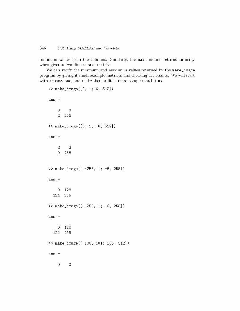
346 DSP Using MATLAB and Wavelets
minimum values from the columns. Similarly, the max function returns an arraywhen given a two-dimensional matrix.
We can verify the minimum and maximum values returned by the make_image
program by giving it small example matrices and checking the results. We will startwith an easy one, and make them a little more complex each time.
>> make_image([0, 1; 6, 512])
ans =
0 0
2 255
>> make_image([0, 1; -6, 512])
ans =
2 3
0 255
>> make_image([ -255, 1; -6, 255])
ans =
0 128
124 255
>> make_image([ -255, 1; -6, 255])
ans =
0 128
124 255
>> make_image([ 100, 101; 106, 512])
ans =
0 0

Applications 347
3 255
As an exercise, generate a random array and verify that the make_image programalways returns results between 0 and 255. Also, try it with floating-point values.What if complex values were passed to this program? How could it be fixed toreturn real integers only?
10.3.1 2D DWT of a Grayscale Image
Now we have our program to show the effects of the 2D DWT on an image. First,we will load the image and show it to the screen.
% load the image
x = imread('dog256x256.gif');
% show the original
figure(1);
imshow(x); title('original image');
Next, we will perform the 2D discrete wavelet transform on the image. Here weuse the Daubechies’ db16 wavelet, though we could use any discrete wavelet thatwe like.
[A, B, C, D] = dwt2(double(x), 'db16');
To make the different subimages viewable, we need to map their values tograyscale pixel values. We use the make_image program from the previous section.
imA = make_image(A);
imB = make_image(B);
imC = make_image(C);
imD = make_image(D);
We need to know how large the subimages are. We can assume that they are thesame size, and create a large image matrix (superx) based on the size of subimageimA. The zeros function simply returns a matrix filled with zeros, with the givendimensions. In this case, the matrix values are all of type uint8.
[MAXA_row, MAXA_col] = size(imA);
% The dimensions should all be the same.
%[MAXB_row, MAXB_col] = size(imB);
%[MAXC_row, MAXC_col] = size(imC);
%[MAXD_row, MAXD_col] = size(imD);
superx = zeros(MAXA_row*2, MAXA_col*2, 'uint8');

348 DSP Using MATLAB and Wavelets
Now we can place the subimages in the four corners of the superx matrix.
% put A in top left
superx(1:MAXA_row, 1:MAXA_col) = imA;
% put B in top right
superx(1:MAXA_row, MAXA_col+1:MAXA_col*2) = imB;
% put C in bottom left
superx(MAXA_row+1:MAXA_row*2, 1:MAXA_col) = imC;
% put D in bottom right
superx(MAXA_row+1:MAXA_row*2, MAXA_col+1:MAXA_col*2) = imD;
Finally, we show the superx matrix as an image.
figure(2);
imshow(superx);
title('After one octave of the DWT');
When we execute this code, we will see an image just like Figure 10.1. Thisworks fine for grayscale images, and we expand this program for color images in thenext section.
10.3.2 2D DWT of a Color Image
We can also perform the 2D DWT of a color image. One way to handle this is totreat the three color components (red, green, blue) as separate signals. We take thisapproach with the code below.
% Perform the DWT of a color image
% first, load and show the image
x = imread('colorimage.jpg');
figure(1);
imshow(x); title('original image');
% Do the 2D DWT on the red component
[Ar, Br, Cr, Dr] = dwt2(double(x(:,:,1)), 'db16');
% Do the 2D DWT on the green component
[Ag, Bg, Cg, Dg] = dwt2(double(x(:,:,2)), 'db16');
% Do the 2D DWT on the blue component
[Ab, Bb, Cb, Db] = dwt2(double(x(:,:,3)), 'db16');

Applications 349
In order to show the results, we must first map the values to the range 0 to 255.We do this for each color component separately.
% Make images from the red DWT results
imAr = make_image(Ar);
imBr = make_image(Br);
imCr = make_image(Cr);
imDr = make_image(Dr);
% Make images from the green DWT results
imAg = make_image(Ag);
imBg = make_image(Bg);
imCg = make_image(Cg);
imDg = make_image(Dg);
% Make images from the blue DWT results
imAb = make_image(Ab);
imBb = make_image(Bb);
imCb = make_image(Cb);
imDb = make_image(Db);
Next, we make a matrix large enough to fit all four subimages. The dimensionsfor the subimages should all be the same, so we base our large matrix’s size on theapproximation. We do not use the original image’s dimensions for this, since the dwtcommand may return extra values according to the boundary. This matrix mustbe three-dimensional, with the third dimension allowing us to differentiate betweenred, green, and blue color components.
% Find the dimensions (which are the same for all subimages).
[MAXA_row, MAXA_col] = size(imAr);
% create a large matrix to put the subimages
superx = zeros(MAXA_row*2, MAXA_col*2, 3, 'uint8');
Now we combine the three color components for the approximation A, and storethem in the large matrix superx.
% put A in top left
superx(1:MAXA_row, 1:MAXA_col,1) = imAr;
superx(1:MAXA_row, 1:MAXA_col,2) = imAg;
superx(1:MAXA_row, 1:MAXA_col,3) = imAb;

350 DSP Using MATLAB and Wavelets
Likewise, we combine the color components for each of the details, and put themin their respective corners.
% put B in top right
superx(1:MAXA_row, MAXA_col+1:MAXA_col*2,1) = imBr;
superx(1:MAXA_row, MAXA_col+1:MAXA_col*2,2) = imBg;
superx(1:MAXA_row, MAXA_col+1:MAXA_col*2,3) = imBb;
% put C in bottom left
superx(MAXA_row+1:MAXA_row*2, 1:MAXA_col,1) = imCr;
superx(MAXA_row+1:MAXA_row*2, 1:MAXA_col,2) = imCg;
superx(MAXA_row+1:MAXA_row*2, 1:MAXA_col,3) = imCb;
% put D in bottom right
superx(MAXA_row+1:MAXA_row*2, MAXA_col+1:MAXA_col*2,1) = imDr;
superx(MAXA_row+1:MAXA_row*2, MAXA_col+1:MAXA_col*2,2) = imDg;
superx(MAXA_row+1:MAXA_row*2, MAXA_col+1:MAXA_col*2,3) = imDb;
Now we show the resulting image.
imshow(superx);
You can find an example image, colorimage.jpg, on the accompanying CD-ROM.From running this program, we see that the approximation retains colors, but thethree details are shades of gray.
10.4 The Plus/Minus Transform
The plus/minus transform is a simple one, used to explain key concepts of thewavelet transform.
Suppose we have the following example signal: 4, 7, 1, 8. We will take everypair of numbers, add them together, and subtract the second one from the first.For the additions/pluses, we have 4+7, and 1+8, resulting in the numbers 11, 9.For the subtractions/minuses, we find 4 − 7 and 1 − 8. The order is important; wealways subtract the second number from the first of every pair. The numbers −3,−7 result from the subtractions. Thus, our transformation gives us two signals:11, 9, and −3, −7.
How can we undo the transform? Suppose we forgot the original numbers, butremember how we got them. We will label the original sequence x1, x2, x3, x4.From the transform, we know:
x1 + x2 = 11

Applications 351
x1 − x2 = −3.
Adding these two equations together gives us:
2(x1) + (x2 − x2) = 11 + (−3) thus,
x1 = (11 − 3)/2 = 4.
We can plug this number into either equation above that has both x1 and x2. Let’suse the first one:
4 + x2 = 11
x2 = 11 − 4 = 7.
So we conclude that the first two original numbers are 4, 7. To find the rest of theoriginal numbers, we repeat the above logic on the next numbers from our signals.This is left as an exercise for the reader.
We saw how the example signal 4, 7, 1, 8 maps to the two signals 11, 9 and−3, −7. Suppose we find the plus/minus transform on each of these resultingsignals:
11 + 9 = 20
11 − 9 = 2 and
−3 + (−7) = −10
−3 − (−7) = 4.
This results in four signals, 20, 2, −10, and 4. We cannot go further, or atleast there is no point in going further due to our data size.
In our plus/minus transform, we add the inputs in pairs then skip to the nextinput pairs. Think of this as shifting the transform over the data. First we find 4+7,then shift over to find 1+8, etc. We could have a transform that involves a largergroup of numbers, but still shift over by two for each calculation. Each level affectsmore of the signal (scaling). For example, level-1 computes 4+7 = 11, involving thefirst two numbers. Level-2 computes (4+7)+(1+8) = 20, where we used the wholesignal. Even if we had a longer signal, we would eventually arrive at a level wherewe use the whole signal. This simple transform shows the shifting and scaling (ofthe index) that exists in the wavelet transform.
To summarize, we have an approximation of 20, and an average of 20/4. Wehave 2 details, level-1: −3, −7 and level-2: 2. Note the similarity to the discretewavelet transform; it has 1 approximation signal, and J detail signals, where J isbased on the input length. If we gave the DWT a signal of four values, we wouldexpect only two possible octaves of resolution, since 22 = 4. This leads us to

352 DSP Using MATLAB and Wavelets
a natural question, “Why should we care about the plus/minus transform?” Toanswer this, first notice that we could multiply through by 1/
√2, to eliminate the
need to divide at the end (i.e., 20/4). If we do this, our plus/minus transformbecomes the Haar transform (from 1910). The plus operation corresponds to thescaling function φ, while the minus operation performs the wavelet function ψ. Witha slight change to our plus/minus transform, we see that it uses coefficients 1/
√2,
1/√
2 and 1/√
2, −1/√
2. A wavelet is a small wave, shifted and scaled, and usedto represent a signal as large, medium, and small waves. The plus/minus transformalso does this.
10.5 Doing and Undoing the Discrete Wavelet
Transform
For signal analysis using the wavelet transform, it makes sense to examine the resultsof the DWT after the transform, but before the signal is completely reconstructed.That is, we can view the signal as a set of subsignals which, when added together,combine to reconstitute the original data. These subsignals are what the wavelettransform removed from the original signal at different levels of resolution.
There are two programs (included on the CD-ROM) specifically for this sort ofanalysis: “DWT undo.m” and “DWT undo2.m,” for the 1D and 2D cases, respec-tively. Both allow the input signal to be analyzed for up to 8 octaves. Keep inmind that the input size limits the number of octaves. If J represents the numberof octaves, then the input signal must be at least 2J samples long (or in the case ofa 2D signal, it must be at least 2J × 2J samples). For both of these programs, thedetails and approximation subsignals are the same size as the original. Comparethese to the normal DWT functions dwt and dwt2, where the size of the subsignalsdepends directly on the octave number. These two programs give the subsignalsas the same size, so that adding all subsignals together recreates the original. Thiswould not be appropriate for a compression application, but extra data is fine foranalysis.
The code below shows how these programs work. First, we will examine the 1Dcase.
x = floor(rand(1,100)*100);
[A, D] = DWT_undo(x, 'db4', 3);
input_recon = A + D(1,:) + D(2,:) + D(3,:);
error = sum(abs(x - input_recon))
The code generates a random signal for x, then finds the DWT and InverseDiscrete Wavelet Transform (IDWT) on x using the db4 wavelet, for three octaves.

Applications 353
The results are returned in a one-dimensional, third-octave approximation A, andthree detail signals D (D(1,:), D(2,:), and D(3,:)). The variable input recon willbe a one-dimensional reconstruction of the original signal x. It should be an exactcopy of x, which we verify in the final statement. Aside from some precision error,the difference between the two signals is zero. The actual output follows.
error =
4.3289e-09
The random signal used above works well to test out the code, but we will runit again with a real signal for x. As the code below shows, we make x a sum ofsinusoids, then apply the “DWT undo” function. When we do, we see that we getthe results as shown in Figures 10.2 and 10.3.
t = 0:0.001:0.1;
x = cos(2*pi*100*t) + 1.5*cos(2*pi*110*t + pi/6);
[A, D] = DWT_undo(x, 'db4', 3);
Figure 10.2 plots the original signal in the top, and the “undone” third-level ap-proximation in the bottom. We see that the signals are the same size, which comesfrom the “DWT undo” function. The approximation signal is not the compact,one-eighth size approximation, but instead the contribution from the approxima-tion channel, ready to be added to the detail contributions sample by sample toreconstruct the original. Keep in mind that we are not after compactness here, butwe want to see how the original signal breaks down into subsignals. Looking at thethree “undone” detail signals in Figure 10.3, we may notice the scale of the detailsgrows according to the octave. The first octave’s detail signal contains many smallvariations, while the second octave’s detail signal has larger variations but fewer ofthem. The second octave’s details would be half the number of the first octave’s,resulting in fewer variations. The larger magnitudes show that the approximationat octave 1 becomes the detail at octave 2. In other words, our idea of “detail”varies (gets larger) with each succeeding octave.
As the details get larger in magnitude from octave 1 to octave 2, so they dobetween octaves 2 and 3. The details at octave 3 contain an interesting feature; wesee the magnitudes get smaller around sample 40 and larger afterwards, just like inthe original signal. In fact, examining the third-octave approximation (bottom plotof Figure 10.2) reveals that before sample 85, the approximation could very easilybe 0. The three detail signals actually contain the salient signal information, atleast before the last few samples.

354 DSP Using MATLAB and Wavelets
10 20 30 40 50 60 70 80 90 100
−2
−1
0
1
2
Original signal
10 20 30 40 50 60 70 80 90 100
−0.5
0
0.5
1
1.5
Approximation at octave 3, undone
Figure 10.2: Results of “DWT undo” for a 1D signal: original and approximation.

Applications 355
10 20 30 40 50 60 70 80 90 100
−0.2
−0.1
0
0.1
0.2
Detail at octave 1, undone
10 20 30 40 50 60 70 80 90 100
−1
0
1
Detail at octave 2, undone
10 20 30 40 50 60 70 80 90 100
−2
0
2
Detail at octave 3, undone
Figure 10.3: Results of “DWT undo” for a 1D signal: details for octaves 1–3.

356 DSP Using MATLAB and Wavelets
Again, we reconstruct the input signal, and compute the error only to find it tobe very small.
>> input_recon = A + D(1,:) + D(2,:) + D(3,:);
>> error = sum(abs(x - input_recon))
error =
3.3799e-10
For the 2D case, let’s start with an image. Any relatively large image will do.We will store it (using double precision) in variable x. Next, we call “DWT undo2”to perform the 2D DWT and IDWT using wavelet db4, for eight octaves. After this,we reconstruct the signal and find the error.
tic
x = double(imread('dog256x256.gif'));
[A, B, C, D] = DWT_undo2(x, 'db4', 8);
y = A;
for k=1:8
tempB(:,:) = B(:,:,k);
tempC(:,:) = C(:,:,k);
tempD(:,:) = D(:,:,k);
y = y + tempB + tempC + tempD;
end
error= sum(sum(abs(x-round(y))))
toc
The output appears below. The commands tic and toc allow us to specify thestart and stop of a virtual stopwatch to know how long the code takes. Note thatthis includes not only the time for “DWT undo2,” but also the time taken by thereconstruction. The total time is just under 17 seconds.
error =
0
Elapsed time is 4.191529 seconds.
Exactly zero error? This comes from the round function, essentially convertingthe reconstructed signal to integer values. As a grayscale image, the original signal’svalues are all integers between 0 and 255, so it makes sense to round the result.

Applications 357
The matrices B, C, andD above store the image details for the number of octavesgiven. That is, B not only contains the detail matrix corresponding to octave 1,it also stores the detail matrix for octaves 2, 3, etc. The differences between B,C, and D are the filters we use to generate each (low-high, high-low, or high-high).These matrices hold the details, and can be used to see edges within the image. Infact, B, C, and D are commonly referred to as the horizontal, vertical, and diagonalcomponents of an image. This is why MATLAB’s documentation (help dwt2) liststhe outputs as “CA, CH, CV, and CD,” for approximate, horizontal, and so forth.
10.6 Wavelet Transform with Matrices
This section will show how the DWT can be computed with matrices. We willconsider only one channel, since the second channel will work the same way andmatrix addition is easy to do. For the second channel, we could either create aseparate matrix or reuse the same one by interlacing the channels or appending oneto the bottom of the other.
First, consider the channel without filter banks. We have two filters along thechannel, an analysis filter h followed by a synthesis filter f . Our transformed dataw will be the input x convolved with h.
w = h ∗ x
Then, we convolve w with f to create our channel output.
output = f ∗ w
So the whole idea here boils down to performing convolution with a matrix operation.Consider a single value, wn from the first convolution. To make things simple, wewill assume that h has four values. Thus,
wn = h3xn−3 + h2xn−2 + h1xn−1 + h0xn.
Notice that this could be accomplished with a 1 × 4 matrix multiplied by a 4 × 1matrix.
wn = [h3 h2 h1 h0]
xn−3
xn−2
xn−1
xn
All we need to do is generalize the h matrix for all n.

358 DSP Using MATLAB and Wavelets
wn
wn+1
wn+2
wn+3...
=
h3 h2 h1 h0 0 0 · · · 00 h3 h2 h1 h0 0 · · · 0
0 0 h3 h2 h1 h0 0...
.... . .
. . .. . .
. . . 00 · · · 0 0 h3 h2 h1 h0
xn−3
xn−2
xn−1
xn
xn+1
xn+2
xn+3...
We can create a similar matrix with f to convolve with w for the other filter.But how do we deal with down-sampling? Surely we do not want to throw away
half of our calculations! The key here is to notice that we only have w values foreven indices n. (Remember that we are considering only the analysis filter for themoment.) In other words, assuming n is even, we want to generate wn, wn+2, wn+4,etc. We can accomplish this by eliminating every other row in the h matrix above.For the matrix as a whole, this appears that we are shifting the h values over bytwo positions every time we go down a row.
wn
wn+2
wn+4
wn+6...
=
h3 h2 h1 h0 0 0 0 0 · · · 00 0 h3 h2 h1 h0 0 0 · · · 0
0 0 0 0 h3 h2 h1 h0 0...
.... . .
. . .. . .
. . . 00 · · · 0 0 0 0 h3 h2 h1 h0
xn−3
xn−2
xn−1
xn
xn+1
xn+2
xn+3...
Now for the up-sampling and reconstruction. Every other input (wn, when n isodd) should be zero.
outputn = f30 + f2wn−2 + f10 + f0wn, n even
outputn = f3wn−3 + f20 + f1wn−1 + f00, n odd
Instead of putting zeros in between w values, we prefer to alter the matrix f . Thisleads us to the following f matrix. Rather than shifting the f values over twicebetween rows, we write them shifted down by two rows between columns. Lookingat the patterns for f and h values, we see the similarity between them and a knight’s

Applications 359
move in a chess game.
outputnoutputn+1
outputn+2
outputn+3...
=
f3 f1 0 0 · · · 00 f2 f0 0 · · · 0
0 f3 f1 0...
0 0 f2 f0 0 00 0 f3 f1 0 0... 0 f2 f0 0
0 · · · 0 f3 f1. . .
wn−6
wn−4
wn−2
wn
wn+2
wn+4
wn+6...
Taking the two matrices, H and G, some interesting properties of these matricesare [3]:
% Daubechies_coeffs.m
%
% Daubechies wavelet coeffs.
%
% Highpass (wavelet) coefficients
d0 = (1-sqrt(3))/(4*sqrt(2));
d1 = -(3-sqrt(3))/(4*sqrt(2));
d2 = (3+sqrt(3))/(4*sqrt(2));
d3 = -(1+sqrt(3))/(4*sqrt(2));
% Lowpass (scaling) coefficients
c0 = -d3;
c1 = d2;
c2 = -d1;
c3 = d0;
H = [c3 c2 c1 c0 0 0 0 0 0 0; ...
0 0 c3 c2 c1 c0 0 0 0 0; ...
0 0 0 0 c3 c2 c1 c0 0 0; ...
0 0 0 0 0 0 c3 c2 c1 c0];
G = [d3 d2 d1 d0 0 0 0 0 0 0; ...
0 0 d3 d2 d1 d0 0 0 0 0; ...
0 0 0 0 d3 d2 d1 d0 0 0; ...
0 0 0 0 0 0 d3 d2 d1 d0];

360 DSP Using MATLAB and Wavelets
disp('multiplying Scaling coeffs by their transpose = I');
H*H.'
disp('multiplying Wavelet coeffs by their transpose = I');
G*G.'
disp('multiplying Scaling coeffs by Wavelet coeffs = 0 matrix');
H*G.'
When we run the above program, we get the following output:
multiplying Scaling coeffs by their transpose = I
ans =
1.0000 0.0000 0 0
0.0000 1.0000 0.0000 0
0 0.0000 1.0000 0.0000
0 0 0.0000 1.0000
multiplying Wavelet coeffs by their transpose = I
ans =
1.0000 0.0000 0 0
0.0000 1.0000 0.0000 0
0 0.0000 1.0000 0.0000
0 0 0.0000 1.0000
multiplying Scaling coeffs by Wavelet coeffs = 0 matrix
ans =
1.0e-17 *
0.3648 -0.1637 0 0
-0.1306 0.3648 -0.1637 0
0 -0.1306 0.3648 -0.1637
0 0 -0.1306 0.3648

Applications 361
From the above run, we see that multiplying a matrix of coefficients by its transposeresults in the identity matrix, i.e., HHT = I, and GGT = I. Also, when we multiplythe two matrices together, we get a zero matrix: HGT = 0. (Do not forget thateach value from the final output above is multiplied by a very tiny exponent. Thesenonzero values can be attributed to precision error.)
This covers only one octave of the wavelet transform. We can extend this to sev-eral octaves, as well as several dimensions. Above, we used the coefficient matricesto define the transform. We can use them recursively to compute further octaves.That is, w = Hx (with H representing the matrix of h values). The other channel’sanalysis would be v = Gx (where G is just like H, except generated from a differentfilter). We will let G represent the matrix made from highpass (wavelet) coefficientsand H represent a similar matrix made from the lowpass (scaling) coefficients. Referto the top of Figure 10.4 for the analysis of x for three octaves.
First, we will find the first level approximation. We will not keep this, but weuse it to compute the other octaves.
approximation1 = Hx
To get the next octave’s approximation, we use the previous result.
approximation2 = Happroximation1
approximation2 = H(Hx)
So the outputs of three octaves of the DWT would be:
detail1 = Gx
detail2 = G(Hx)
detail3 = G(H(Hx))
approximation3 = H(H(Hx)).
We can calculate these values recursively, as above, or we can create transformmatrices that have the same result.
10.7 Recursively Solving a Su Doku Puzzle
Su Doku is a puzzle where digits 1 through 9 appear exactly once in every row,column, and 3 × 3 submatrix. The puzzle comes with some of the numbers alreadyfilled in, and the object is to fill in the rest. For example, imagine a row with the

362 DSP Using MATLAB and Wavelets
Detail 2
LPF 2LPF 2
HPF 2
HPF 2LPF 2
HPF 2Input
X[n]
IHPF2
ILPF2ILPF2
IHPF2ILPF2
2 IHPF
Y[n]
OutputDetail 1
Detail 2
Detail 3
Approximate
Analysis (Forward Transform)
Synthesis (Inverse Transform)
The wavelet transform shown for 3 octaves (resolution levels)
Detail 1
Detail 3
Approximate
Figure 10.4: Three octaves of the one-dimensional discrete wavelet transform.

Applications 363
Table 10.1: An example Su Doku puzzle.
0 2 3 4 0 6 7 8 04 0 6 7 0 9 1 0 37 8 0 1 0 3 0 5 6
3 1 2 0 0 0 9 7 80 0 0 0 0 0 0 0 06 9 8 0 0 0 5 1 4
2 7 0 3 0 8 0 9 19 0 1 6 0 2 8 0 50 6 4 9 0 5 2 3 0
first eight numbers given as 3, 1, 5, 9, 7, 6, 8, 4 followed by a blank. We knowthat the number that goes in the blank cannot be a repeat of any of the numbersalready in the row, and by the process of elimination we arrive at the conclusionthat 2 must go in the blank spot. With similar logic, we should be able to completethe puzzle. A well-constructed Su Doku puzzle has only one solution. But how dowe know if this is the case?
We can treat the puzzle as a matrix, and use MATLAB to solve it for us. Sure,this takes the fun out of it, but we will go one step further: we will have MATLABfind all possible solutions.
To solve this problem, we will use recursion. We start with the puzzle in anincomplete form, with 0s for the blanks. Next, we will find the first blank (zero),and put a guess in its place. We then check to see if our guess causes a problem;if this number already exists in the row, column, or 3 × 3 submatrix. If a conflictexists, we repeat the process with a new guess. To keep it simple, our guesses willalways start with 1, then increment to 2, then increment to 3, and so forth until wereach 9.
Table 10.1 shows an example Su Doku puzzle with 0s in the place of blanks.Table 10.2 gives the answer. If you have not seen this puzzle before, see if you cansolve it on your own.
To solve the problem, we will use three MATLAB files: a program to give the in-complete puzzle and start things off, a function to check to see if the puzzle is valid,and a function to look for blanks and fill them in with guesses. We will call the start-ing program sudoku.m, then the function that checks the puzzle sudoku_check.m,and the search and guess function sudoku_search.m.
First, let’s look at the starting program. We define the puzzle as a matrix, with

364 DSP Using MATLAB and Wavelets
Table 10.2: The example Su Doku puzzle’s solution.
1 2 3 4 5 6 7 8 94 5 6 7 8 9 1 2 37 8 9 1 2 3 4 5 6
3 1 2 5 6 4 9 7 85 4 7 8 9 1 3 6 26 9 8 2 3 7 5 1 4
2 7 5 3 4 8 6 9 19 3 1 6 7 2 8 4 58 6 4 9 1 5 2 3 7
zeros in place of the blanks. We next check out the puzzle, to make sure it is valid,using the sudoku_check function. If it is not, the search function will never find asolution, so we look for this up front. Then we call our sudoku_search function.
puzzle = [ 0, 2, 3, 4, 0, 6, 7, 8, 0;
4, 0, 6, 7, 0, 9, 1, 0, 3;
7, 8, 0, 1, 0, 3, 0, 5, 6;
3, 1, 2, 0, 0, 0, 9, 7, 8;
0, 0, 0, 0, 0, 0, 0, 0, 0;
6, 9, 8, 0, 0, 0, 5, 1, 4;
2, 7, 0, 3, 0, 8, 0, 9, 1;
9, 0, 1, 6, 0, 2, 8, 0, 5;
0, 6, 4, 9, 0, 5, 2, 3, 0]
if (sudoku_check(puzzle))
sudoku_search(puzzle);
end
The function that checks the puzzle appears below. It works simply by isolatingeach row, and counting the occurrence of each of the numbers 1 through 9. If itfinds more than one occurrence of a number, then it sets the OK flag to false
to indicate that the puzzle has an invalid entry. Next, we check each column in asimilar way. Finally, we check every submatrix. Once the function completes, itreturns the OK flag. The calling program hands sudoku_check.m a puzzle, and itgives back a simple true or false value. Rather than show the whole function, we

Applications 365
will show just the first part that checks each row. See the function listing on theCD-ROM for the checks on the columns and submatrices.
% sudoku_check.m
%
% Check a Su Doku puzzle -
% make sure each number appears in only one row,
% column, and 3x3 submatrix.
%
function OK = sudoku_check(puzzle)
% assume the puzzle is OK, until we find otherwise
OK = true;
% Check to see if the puzzle matrix is good
% First, check along the rows. r = row number
for r = 1:9
% Isolate one row of the puzzle
row = puzzle(r, 1:9);
% let n be the number (1..9)
for n = 1:9
% initialize count for this number
num_count = 0;
% examine each column
for c = 1:9
% if the puzzle entry matches the number
% we are looking for, add one to the count.
if (row(c) == n)
num_count = num_count + 1;
end
end
% make sure every number 1..9 appears <= 1 time
if (num_count > 1)
% we found a duplicate in this row
OK = false;
end
end
end
% See sudoku_check.m for the column check
% and the 3x3 submatrix check

366 DSP Using MATLAB and Wavelets
Our goal is to show all possible solutions. Since we do not need to keep thesolutions that we find, we will simply print them to the screen. The sudoku_searchfunction finds the blanks, and if it does not find a blank, it prints the puzzle.
This search function receives a puzzle matrix which may or may not be complete.It sets up a variable called blank that we use to indicate the presence of one or moreblanks in the puzzle. Actually, we do not care how many blanks there are, we justwant to know if there is one. So we assume there are no blanks, then look throughthe matrix. If we find one, we update our blank variable to indicate this, and goon to the next part. If we find a blank in the first spot that we look, why shouldwe bother looking through the rest of the puzzle? This explains why we use while
loops instead of for loops; we might want to exit the loops early.In the next part, there are two possibilities. Either we found a blank and exited
the loops early, or we looked through the whole puzzle and did not find one. Weassume that all puzzles passed to the search function are valid, so if there are noblanks, then we must have a solution. In this case, we print the matrix and exit thefunction. If we found a blank, then we want to try a guess in that position. Oncewe have a guess in place, we check to make sure the guess is valid. Just because itis valid does not mean that it will be part of the solution; we may find that it leadsto a contradiction later. For example, looking at the puzzle in Table 10.1, we seethe upper-left corner has a blank, and that both 1 and 5 are valid possibilities here.But only one of these possibilities is the correct answer.
When we have a valid guess in our puzzle, we need a way to search for moreblanks, and fill them in. (Doesn’t this sound familiar?) This is where recursioncomes in; the search function calls itself with the updated puzzle! The computerkeeps track of the functions that we call, and allows us to call a function from withinitself. Of course, we have to be careful here—done carelessly, the function could callitself over and over again indefinitely, possibly crashing the computer as a result.Our solution will work because we take a step in the right direction every time wecall our search function. There are many possible calls we could make, but they arefinite. We can even start with a matrix of zeros, and the computer will print everypossible Su Doku solution.
Our solution also rests on the fact that the search function has a function
keyword in its definition. The computer will keep a copy of its data separate fromother functions. It allocates variables as needed, then gets rid of these variables whenthe function quits. Instead of there being one matrix called puzzle, there are actuallymany of them depending on how many calls we have made to sudoku_search. Allthese different versions of the puzzle work to our advantage, since they allow back-tracking by the computer. That is, if the search function inserts a bad (but valid)guess, it will call itself with that guess in place. If the next call of the search

Applications 367
function cannot make the puzzle work, control will come back to the previous call ofthe function, and it can try a new guess. The code for the search function appearsbelow.
%
% sudoku_search
%
% Try to recursively fill out a Su Doku puzzle.
%
function blank = sudoku_search(puzzle)
% assume that there are no blanks,
% until we find one
blank = false;
% Part I:
% look through the puzzle, until we find a blank
% or get to the last puzzle position
row = 1;
% examine the rows
while ((row <= 9) && (~blank))
% examine every column
col = 1;
while ((col <= 9) && (~blank))
% Does the puzzle have a blank?
if (puzzle(row,col) == 0)
blank = true;
else
% Go to next column
col = col + 1;
end
end
% Go to next row, unless we are done.
if (~blank)
row = row + 1;
end
end
% Part II:
% Did we find a blank?

368 DSP Using MATLAB and Wavelets
if (blank)
% found a blank to fill in,
% so try all values 1..9
for value=1:9
% Try the current value there
puzzle(row,col) = value;
% maybe this value is already in this row,
% or in this column, or 3x3 submatrix ?
if (sudoku_check(puzzle))
% the value does not cause a problem
% so try to fill in any remaining blanks
sudoku_search(puzzle);
end
end
else
% Show the puzzle if no blanks were found.
% That is, we know the puzzle checks out
% (or this function would not have been called),
% so if no blanks are left, then we have a
% solution!
puzzle
end
Recursion allows the programmer to solve a complex problem by writing a rel-atively small function. First, a recursive function checks to see if it is done. If not,it takes the problem one step closer to the solution and calls itself. We could havewritten the search function in a way that does not use recursion, but then we wouldhave to keep track of what changes we made to the puzzle and implement our ownmechanism to undo changes as needed.
Now that we have seen how the puzzle should work, let’s see an example thatdoes not work so well. In the example puzzle above, we have 4 as the first entry onthe second row. But what if we replace this with a blank? We will test it out withthe program.
>> puzzle = [ 0, 2, 3, 4, 0, 6, 7, 8, 0;
0, 0, 6, 7, 0, 9, 1, 0, 3;
7, 8, 0, 1, 0, 3, 0, 5, 6;
3, 1, 2, 0, 0, 0, 9, 7, 8;
0, 0, 0, 0, 0, 0, 0, 0, 0;
6, 9, 8, 0, 0, 0, 5, 1, 4;

Applications 369
2, 7, 0, 3, 0, 8, 0, 9, 1;
9, 0, 1, 6, 0, 2, 8, 0, 5;
0, 6, 4, 9, 0, 5, 2, 3, 0]
>> sudoku_search(puzzle);
Shortly afterwards, MATLAB responds with the following output.
puzzle =
1 2 3 4 5 6 7 8 9
4 5 6 7 8 9 1 2 3
7 8 9 1 2 3 4 5 6
3 1 2 5 6 4 9 7 8
5 4 7 8 9 1 3 6 2
6 9 8 2 3 7 5 1 4
2 7 5 3 4 8 6 9 1
9 3 1 6 7 2 8 4 5
8 6 4 9 1 5 2 3 7
puzzle =
1 2 3 4 5 6 7 8 9
5 4 6 7 8 9 1 2 3
7 8 9 1 2 3 4 5 6
3 1 2 5 6 4 9 7 8
4 5 7 8 9 1 3 6 2
6 9 8 2 3 7 5 1 4
2 7 5 3 4 8 6 9 1
9 3 1 6 7 2 8 4 5
8 6 4 9 1 5 2 3 7
As we see from the output, the puzzle now has two solutions. Examining the twosolutions shows that the columns 1 and 2 in rows 2 and 5 are the only differences.
10.8 Converting Decimal to Binary
To convert a decimal number to binary, most people are familiar with a divide-by-two algorithm. We start with the decimal number and divide by 2, keeping track of

370 DSP Using MATLAB and Wavelets
Table 10.3: Converting from decimal to binary.
number number / 2 remainder
38 19 0
19 9 1
9 4 1
4 2 0
2 1 0
1 0 1
the remainders (which must be either 0 or 1). Repeat this until we get zero for theresult. Then we write these remainders from the bottom to the top.
For example, suppose we want to convert the number 38 to binary. As we cansee from Table 10.3, the remainders (in reverse order) are 100110. Since we havenot established how many bits we use in storing the fixed-point binary number,and because the left-most bit typically indicates sign, we append a zero to the leftto avoid confusion. This gives us 0100110 as our answer. We can check this byconverting it back to decimal: 32 + 4 + 2 = 38.
This assumes that the decimal number is positive. When it is negative, use theabsolute value instead. At the end, convert all 0s to 1s and all 1s to 0s, then add 1.Keep in mind that 1 + 1 = 10 in binary. This final step (called two’s complement)returns the correct bit pattern for negative numbers. We will not worry aboutnegative numbers below, since the floating-point standard uses a sign bit instead ofusing two’s complement.
But what if we wanted to convert 38.1 to a fixed-point binary representation? Wealready know the bits to the left of the radix point, and we use a similar algorithmto find the fractional part.
We will start with the fractional number, multiply by 2 (or, if you prefer to thinkof it this way, divide by 2−1), and keep track of the whole part. We repeat this withthe fractional part of the previous number until we get a zero for the fractional part.
Notice that in Table 10.4 the last fractional number, 0.4, was already seen in thetable. This fractional part does not have a compact binary representation. Instead,like the number 1/3 in decimal, it repeats forever. The best we can do is store anapproximation of .00011.
Using these two decimal-to-binary techniques together, we conclude that 38.1

Applications 371
Table 10.4: Converting from a decimal fraction to fixed-point binary.
fractionalnumber number × 2 whole part
0.1 0.2 0
0.2 0.4 0
0.4 0.8 0
0.8 1.6 1
0.6 1.2 1
0.2 0.4 0
converted to fixed-point binary is:
0100110.00011.
What if we want to store this value as a floating-point number? The Instituteof Electrical and Electronics Engineers has a standard for floating-point storage in32 or 64 bits, commonly called the IEEE 754 standard [38]. We break the binaryrepresentation into three fields: the sign bit, the significand, and the exponent.(The significand may also be called by the older name of mantissa.) In other words,the number appears as ±significand×2±exponent. Of course, the size of the storageword directly affects precision; in the IEEE 754 standard, we label the precisionthe number of bits used to represent the significand. As the example above shows,the significand that we store depends upon the precision. With 32 bits for theentire floating-point representation (called single precision), we use 23 bits for thesignificand. When we have a 64-bit word (double precision), we use 52 bits for it.One bit stores the sign, and the remaining bits store the exponent. Therefore, theexponent will consist of 8 or 11 bits, according to the precision.
You may also see the precision given as 24 bits and 53 bits, respectively. Theone bit difference comes from the “hidden” bit, which is not explicitly stored [38].Remember that the significand consists only of 0s and 1s, and the magnitude of eachbit depends on the exponent. For example, 0.1×20 has the same value as 1.0×2−1.We can always make the first bit a 1 by altering the exponent, so why not requireit? This way, we do not need to store that bit. The IEEE 754 standard uses thisstrategy.
One final note about the IEEE 754 standard is that the exponent ranges from−126 to +127 (for an 8-bit exponent), or −1022 to +1023 (for 11-bit exponents).

372 DSP Using MATLAB and Wavelets
The computer stores these exponents with a bias of 127 and 1023, respectively. Tofind the actual exponent value to use, we subtract the bias value from the valuestored. For example, suppose the stored exponent value for a 32-bit floating-pointvalue is 10000011 in binary, or 131 in decimal. The actual exponent would be131 − 127 = 4, so the number in the significand is multiplied by 24.
With 126 possible negative exponent numbers, 127 positive numbers for theexponent, and 1 number for a zero exponent, we have 254 possible values. Theother two possibilities allow for special meanings, such as a zero significand whenall exponent bits are 0. Otherwise, the bits stored in the significand would beinterpreted as starting with a hidden 1.
Let’s create a double value and print it to the screen in hexadecimal. Theformatting string in the sprintf command may be a bit daunting. The percentsign indicates that a variable should be printed, as in the programming language C.The x and \n are standard C-like formatting, meaning hexadecimal and new-line,respectively. We could do without the \n, but it gives us a nice space before thenext MATLAB prompt. The final formatting parameter b tells MATLAB to use adouble type. Thus, we see the double values as hexadecimal strings that can easilybe converted to binary with a lookup chart.
>> disp(sprintf('%bx \n',0.0))
0000000000000000
>> disp(sprintf('%bx \n',-0.0))
8000000000000000
>> disp(sprintf('%bx',38.1))
40430ccccccccccd
We see from the above MATLAB output that zero and negative zero are actuallystored in two different ways! MATLAB takes care of this for us, as the followingcode shows.
if (-0.0 == 0.0)
disp('equal');
else
disp('not equal');
end
When we run it, we see that MATLAB behaves as we expect.
equal

Applications 373
In other words, though zero and negative zero have different internal represen-tations, MATLAB will treat them as equal.
Let’s do one more example of a number stored in the IEEE 754 standard. Noticethe t parameter that says to treat the number as a 32-bit floating-point value.
>> disp(sprintf('%tx',16.875))
41870000
We can use the chart in Table 10.5. (As a side note, you may see hexadecimalvalues in either uppercase or lowercase. For example, 1a3f is the same as 1A3F.)Writing out the binary values, we have:
hex: 4 1 8 7 0 0 0 0binary: 0100 0001 1000 0111 0000 0000 0000 0000 .
Now we rewrite the binary string, according to the floating-point standard.
sign exponent significand0 10000011 00001110000000000000000
The interpretation is positive for the sign. For the exponent we have 100000112 =13110, subtracting the bias we get 131−127 = 4. With the hidden bit, the significandbecomes 1.0000111. The result is +1.0000111 × 24, or simply 10000.111. If weconvert the left half to decimal, we find it is 24 = 16. The right half converts to2−1 + 2−2 + 2−3 = .875, so the original number must be 16.875, just like in theprevious sprintf statement.
10.9 Frequency Magnitude Response of Sound
The following program plots the frequency magnitude response of sound. Since itrepeats itself in a loop, the graph appears to change in (almost) real time.
The first few lines set up the variables to save time later. This includes an arraythat we will use to show only the first half of the frequency information, as wellas another array for the x-axis, to show it in terms of actual frequencies instead ofsample number.
% show_sound.m
%
% Get the FMR of a sound
%

374 DSP Using MATLAB and Wavelets
Table 10.5: Hexadecimal to binary chart.
hexadecimal decimaldigit binary equivalent
0 0000 0
1 0001 1
2 0010 2
3 0011 3
4 0100 4
5 0101 5
6 0110 6
7 0111 7
8 1000 8
9 1001 9
a 1010 10
b 1011 11
c 1100 12
d 1101 13
e 1110 14
f 1111 15

Applications 375
figure(1); % bring figure 1 to the front
fs = 44100;
N = 4410*1;
half = 1:ceil(N/2);
MaxFreq = ceil(max(half)*fs/N);
xaxis = half*fs/N;
Next, we try to use the audiorecorder feature of MATLAB. Either it will besupported, or the program will later try to use the wavrecord instead. The code isnot perfect, though, since some computers with an older version of MATLAB willnot be able to use the wavrecord function either.
% detect if we should use audiorecorder
try
audiorec = 1;
x_object = audiorecorder(44100, 16, 1);
catch
audiorec = 0;
disp('No audiorecorder support.');
end
The heart of the program is a for loop that records sound then displays it onscreen. The pause command must be in place to give the system a chance to updatethe screen. The other commands simply make the plot look nice and consistent.
for i=1:10
% record some sound
if (audiorec)
recordblocking(x_object, 0.5);
% find FFT's magnitudes
X = abs(fft(getaudiodata(x_object, 'double')));
else
x = wavrecord(N, fs, 1);
% find FFT's magnitudes
X = abs(fft(x));
end
% plot the FMR
plot(xaxis, X(half));
% make the plot look good

376 DSP Using MATLAB and Wavelets
axis([0 MaxFreq 0 100]);
xlabel('Frequency (Hz)');
ylabel('Amplitude');
title('Frequency Magnitude Response for sound');
% Give the system time to show the graph
pause(0.01);
end
When running, the program records sound and shows its frequency magnituderesponse (FMR) as quickly as possible. To make it run longer, simply adjust thenumbers in the for line. Also, users with both wavrecord support and a laterversion of MATLAB may want to try both recording functions. The wavrecord
function allows a smaller interval of recording time to make the program seem torun in real time.
Figure 10.5 contains an example of the program’s output, where the microphone’sinput is a whistle sound. As the program runs, the graph changes according to theinput signal. With this program, we can see how simple sounds (like the whistle)appear in the frequency-domain, or look at more complex signals, such as speech.If a musical instrument is played nearby, the harmonics from the notes will show upas spikes in the frequency-domain.
10.10 Filter Design
We saw how various filters affect a signal. But how does one determine the filtercoefficients to use, to achieve a certain effect? We examine FIR filter design in thissection.
10.10.1 Windowing Methods
MATLAB provides the fir1 function to design FIR filters in the Signal Processingtoolbox. As its documentation points out, this function uses the windowing method.This means that the filter coefficients have a gradual rise based on the window given,to minimize the ill-effects cause by sudden transitions. For example, consider thecode below. We have an impulse function x, filtered by two different filters. Thefirst step is to make the impulse function.
imp = zeros(1, 1000);
imp(50) = 1;
Now we will filter this with filter coefficients 1, 1, 1, 1, 1. Once filtered, weshow the frequency magnitude response.

Applications 377
0 0.5 1 1.5 2
x 104
0
10
20
30
40
50
60
70
80
90
100
Frequency (Hz)
Am
plitu
de
Frequency Magnitude Response for sound
Figure 10.5: Example of the “show sound” program.

378 DSP Using MATLAB and Wavelets
myfilt = [1, 1, 1, 1, 1];
y = conv(imp, myfilt);
Y = fft(y);
maxY = max(abs(Y));
half = 1:ceil(length(y)/2);
subplot(2,1,1);
plot(half, abs(Y(half))/maxY, 'b');
title('FMR for filter coeffs [1, 1, 1, 1, 1]');
axis tight;
We can compare this to the effect of another filter, one where the filter coefficientsmore gradually approach 1, then gradually fall.
myfilt2 = [1/3, 2/3, 1, 2/3, 1/3];
y2 = conv(imp, myfilt2);
Y2 = fft(y2);
maxY2 = max(abs(Y2));
subplot(2,1,2);
plot(half, abs(Y2(half))/maxY2, 'b');
title('FMR for filter coeffs [1/3, 2/3, 1, 2/3, 1/3]');
axis tight;
From the graph, shown in Figure 10.6, we see that both sets of filter coefficientsproduce a lowpass filter. However, the top graph shows a sizeable side lobe where thefrequency response becomes larger and then smaller. While the frequency responseis very small around index 200, we see that it becomes much larger after this point.On the other graph, we see the frequency response approach zero a bit more slowly(we say it has a wider main lobe). We also see that it has a much smaller sidelobe. These graphs demonstrate the effect of a window; in fact, the second filter’scoefficients were chosen from the simple “triangle” window. In other words, the firstset of filter coefficients were “windowed” to make the second set.
The command below returns the 5-value “triangle” window function. Note thatthe window function is part of the optional Signal Processing toolbox in MATLAB.
>> w = window(@triang, 5)
w =
0.3333
0.6667

Applications 379
50 100 150 200 250 300 350 400 450 500
0.2
0.4
0.6
0.8
1FMR for filter coeffs [1, 1, 1, 1, 1]
50 100 150 200 250 300 350 400 450 500
0.2
0.4
0.6
0.8
1FMR for filter coeffs [1/3, 2/3, 1, 2/3, 1/3]
Figure 10.6: Two similar filters, with and without a gradual transition.

380 DSP Using MATLAB and Wavelets
1.0000
0.6667
0.3333
Now that we have an idea about how windows apply to filter coefficients, wereturn to the topic of FIR filter design. If we have an impulse function in the time-domain, we need an infinite number of frequency-domain values to represent it. Thereverse is also true; a frequency-domain impulse requires an infinite number of time-domain points. To make a time-domain filter, we decide how its frequency-domainresponse should look. We can control the cutoff frequency, that frequency abovewhich a lowpass filter starts zeroing out frequency content. Ideally, this would be abinary function where all frequency content below the cutoff would remain the samewhile content above the cutoff would be zero. In practice, the best we can hope foris a steep slope. We can also control how many filter coefficients we have, called thetaps or order. (The order equals number of taps minus 1.) So, to make a reasonablecompromise, we window the filter coefficients to the number of taps given. Morecoefficients give a frequency response that better approximates the ideal, but at theexpense of more processing (be it more software processing or more hardware areaneeded to implement the filters).
10.10.2 Designing an FIR Filter
Let’s try to design an FIR filter. We will start with the frequency response thatwe want, and work from there. For simplicity, we will have a lowpass filter with acutoff frequency at 30%. We need an impulse function to work with, so we defineand use imp. We will use the length MAXLEN a few more times, so we might aswell define it now.
% create an impulse function
MAXLEN = 1000;
imp = zeros(1, MAXLEN);
imp(50) = 1;
Next, we need to define our cutoff frequency in terms of how many frequency-domain values to use; 150 out of 500 corresponds to 30%, so we will use this. (The500 comes from half the spectrum size of MAXLEN.) Also, we will define the numberof coefficients to use.
low_pass_end = 150;
taps = 51;

Applications 381
We simulate the response we want in the frequency-domain as an ideal function,fx. Most of the response should be zero, with the lower end including ones. Thatis, the filter should allow the bottom 30% of frequencies to pass through. Also, weset the top half of the ideal function fx as a mirror image of the bottom half, as wewould expect for a frequency magnitude response of a real-valued function. (Thiscorresponds to the top half of the frequency magnitude response that we do notplot.)
fx = zeros(1, MAXLEN);
fx(1:low_pass_end) = 1; % lowpass
% include mirror image of lowpass
fx((MAXLEN-low_pass_end):MAXLEN) = 1;
Once we have our ideal frequency response specified, we convert it to the time-domain. We shift it to move the center around the midpoint, instead of around zero.We can do this since the magnitudes of the frequency-domain data would remainthe same, only the phases would change (see the material on DFT shifting theory,section 6.5).
% convert to time-domain
x = ifft(fx);
% shift frequency data
mid_point = floor(MAXLEN/2);
x2 = [x(mid_point+1:MAXLEN), x(1:mid_point)];
We get the requested number of filter coefficients by taking an equal number frombefore the midpoint and after the midpoint. Including the midpoint, we have anodd number of filter coefficients (which explains why we selected 51 for the numberof taps above).
half_taps = floor((taps-1)/2);
b2 = x2(mid_point - half_taps : mid_point + half_taps);
The variable b2 stores the filter coefficients that we want to use. However, wecannot use them directly, since they are complex values. We may be tempted touse the abs function to convert them to real values, but then they would all bepositive. To preserve the signs, we can examine each value and store its sign as wellas magnitude. In the process, we create a new variable c2 to hold these values.
for k=1:length(b2)

382 DSP Using MATLAB and Wavelets
if (sign(b2(k)) < 0)
c2(k) = -abs(b2(k));
else
c2(k) = abs(b2(k));
end
end
Finally, we have filter coefficients that we can use. Here we omit the details forplotting these coefficients and the resulting frequency magnitude response, but theprogram filter_test2.m contains the commands. Figure 10.7 shows the results.
5 10 15 20 25 30 35 40 45 50
0
0.1
0.2
0.3filter coeffs (nonwindowed)
10 20 30 40 50 60 70 80 90 100
0.2
0.4
0.6
0.8
1FMR for filter, using ifft to generate filter coeffs
Figure 10.7: Using nonwindowed filter coefficients.
As we see from Figure 10.7, the frequency magnitude response contains ripples.We saw that windowing can reduce these ripples, so we will next improve our filtercoefficients with a window. Here we use a Hamming window, one of many possiblechoices. With the window w, we multiply each value in c2 to create a new set offilter coefficients, d2. You may notice the transpose on the window w; this simply

Applications 383
changes it from a column vector to a row vector so that the .* operation does nothave a problem with a mismatch of matrix dimensions.
w = window(@hamming, taps);
d2 = w.' .* c2;
Figure 10.8 shows the new filter coefficients and an improved frequency magni-tude response. At first glance, the filter coefficients shown in this figure look justlike the ones in Figure 10.7. The differences are best seen in the first 10 and last 10filter coefficients. The frequency magnitude response looks much better in Figure10.8 since the ripples have been smoothed out. (The ripples are still there, justgreatly reduced, as a logarithmic plot would show.)
5 10 15 20 25 30 35 40 45 50−0.05
0
0.05
0.1
0.15
0.2
0.25
filter coeffs with window
10 20 30 40 50 60 70 80 90 100
0.2
0.4
0.6
0.8
1FMR for filter, using ifft + window to generate filter coeffs
Figure 10.8: Using windowed filter coefficients.
Now let’s see what the fir1 command will do for us. Here we ask for the samenumber of filter coefficients, with the same cutoff frequency (30%). We requesttaps − 1 coefficients, since the function expects the order. That is, starting the

384 DSP Using MATLAB and Wavelets
count from 0, the order is the highest index value. So the fir1 will return one morecoefficient than we specify.
b1 = fir1(taps-1, 0.3);
Figure 10.9 shows the two sets of filter coefficients and their respective frequencymagnitude responses. The filter coefficients look very similar (and are very similar invalue), even though they are not lined up. For the frequency magnitude responses,we see the plots are on top of one another. To really see a difference, we would needa logarithmic plot.
5 10 15 20 25 30 35 40 45 50
0
0.1
0.2
0.3filter coeffs
10 20 30 40 50 60 70 80 90 100
0.2
0.4
0.6
0.8
1FMR for filters, ifft + window vs fir1
Figure 10.9: Windowed filter coefficients and those generated by fir1.
Our example FIR filter coefficients closely match the ones generated by thefir1 function in MATLAB. From this discussion, you should be able to generatecoefficients for any lowpass filters you want simply by changing the parameters(number of taps and cutoff frequency). But what if you do not want a lowpassfilter? Multiplying the filter coefficients by a sinusoid has the effect of moving thefrequency magnitude response in the frequency-domain.

Applications 385
A high-frequency sinusoid would jump from −1 to +1, which we simulate. Afinal modification of the filter coefficients will be to apply an alternating flip to thesign of the values.
f2 = d2;
flip = 1;
% flip every other sign
for k=1:length(f2)
if (flip == 1)
f2(k) = -f2(k);
flip = 0;
else
flip = 1;
end
end
When we run this code, our filter coefficients will appear as in Figure 10.10. Asthe frequency magnitude response shows, the filter now attenuates low frequenciesand passes the high frequencies. Thus, we have created a highpass filter. We canalso have MATLAB give us a highpass filter, again with the fir1 command. Noticehow we use 0.7 instead of 0.3 for the cutoff. What would be the result if we left itas 0.3?
b3 = fir1(taps-1, 0.7, 'high');
This section gives an overview of windowing functions, and shows why they areuseful. Also, we explored making our own FIR filters both with a MATLAB SignalProcessing toolkit command, as well as our own program. Though this programuses the window command, also part of the Signal Processing toolkit, it should beclear to the reader how this could be done without that toolkit.
10.11 Compression
Compression programs take the redundancy out of data to store it in a compact form.There are lossy compression algorithms, that tolerate some loss of information. Forexample, the popular JPEG and MP3 compression standards (files with extensionsof .jpg and .mp3, respectively) do not return an exact copy of the original to theuser, but a version close enough to the original that the user should not noticethe difference after uncompressing it. Another possibility is a lossless compressionalgorithm. Programs such as gzip and winzip store data compactly, but do not lose

386 DSP Using MATLAB and Wavelets
5 10 15 20 25 30 35 40 45 50
−0.2
−0.1
0
0.1
0.2
filter coeffs (every other sign changed)
10 20 30 40 50 60 70 80 90 100
0.2
0.4
0.6
0.8
1FMR for filter, using ifft + window + alt. flip for filter coeffs
Figure 10.10: Alternating flip for the windowed filter coefficients.

Applications 387
any information in the process. Obviously, there are times when a lossy compressionworks well, such as with images for a Web page, and other times when a losslesscompression program should be used instead, like when storing a program or word-processing document.
JPEG stands for Joint Photographic Experts Group. This group has set a coupleof standards for images, namely the “basic” JPEG standard and JPEG 2000 (withextension .jp2).
There are three steps to compression algorithms, namely transformation, quan-tization, and entropy coding. Applying a transform should remove some of theredundancy in the data. Quantization maps the data to a set number of values,such as rounding the transformed data to the nearest integer. Of course, data maybe lost in this step. The final compression step, entropy coding, represents thequantized data in a compact way. This is much like the way people communicatewith instant messenger applications; why spell out “how are you doing today” when“hw RU 2day” gets the idea across in less than half the number of characters?
10.11.1 Experimenting with Compression
Let’s experiment with an image to see how JPEG compression affects an image.First, we need a suitable noncompressed image. The code below uses a file calledPIA02187.tif, an image from the planet Mars. (This image was obtained fromNASA’s Jet Propulsion Laboratory,http://photojournal.jpl.nasa.gov/targetFamily/Mars, posted on February 17, 2006.)The .tif extension means that the image follows the TIFF (Tagged Image FileFormat) standard. TIFF files may be compressed, or may be stored as “raw” data.The command below reads the image and stores it in the uint8 array original. Thefilename comes first, followed by the file type.
original = imread('PIA02187.tif', 'TIFF');
If you are not able to locate this image, any suitable, uncompressed, grayscaleimage should work.
Next, we save the image as several different files. The imwrite command takesthe variable storing the image data as the first parameter, followed by the name ofthe file to create, then the type of image format to use. The last two parametersspecify that the optional parameter “Quality” should be set to the number given,up to 100. We will use the term “image of quality 25” to refer to the image storedin the last line below. The number does not really indicate quality, but refers onlyto the parameter passed to the imwrite function.
imwrite(original, 'PIA_100.jpg', 'JPEG', 'Quality', 100);

388 DSP Using MATLAB and Wavelets
imwrite(original, 'PIA_75.jpg', 'JPEG', 'Quality', 75);
imwrite(original, 'PIA_50.jpg', 'JPEG', 'Quality', 50);
imwrite(original, 'PIA_25.jpg', 'JPEG', 'Quality', 25);
We will momentarily use the file sizes to tell us about the compression. But weshould not compare the JPEG images to the TIFF image, since these two differentformats vary. Our purpose is not to compare the two different formats, but toinvestigate the compression and quality of one image. Therefore, we need to storethe image in a lossless fashion. Note that the image may still be compressed (storedin a compact way), but without losing information. Fortunately, storing the imageas a lossless JPEG is easy, as the command below demonstrates.
imwrite(original, 'PIA_noloss.jpg', 'JPEG', 'Mode', 'lossless');
We can check on the files from the MATLAB prompt. The ls command (anddir command) work like they do from a command-line interface (such as a terminalwindow under Linux, Unix, and OS X, or the command.exe program under MicrosoftDOS or Windows). Related commands like cd (change directory), pwd (printworking directory), and mkdir (make directory) are also supported.
>> ls -l PIA*
-rw-r--r-- 1 mweeks staff 1446095 Feb 17 18:41 PIA02187.tif
-rw-r--r-- 1 mweeks staff 1074473 Feb 17 18:45 PIA_100.jpg
-rw-r--r-- 1 mweeks staff 142951 Feb 17 18:45 PIA_25.jpg
-rw-r--r-- 1 mweeks staff 209001 Feb 17 18:45 PIA_50.jpg
-rw-r--r-- 1 mweeks staff 298521 Feb 17 18:45 PIA_75.jpg
-rw-r--r-- 1 mweeks staff 978460 Feb 17 18:45 PIA_noloss.jpg
As we see from the output, the file sizes are 1.4 megabytes for the original, 140kilobytes for the compressed one with a quality of 25, 204 kilobytes and 291 kilobytesfor the compressed files with qualities 50 and 75, respectively. It should be obviousthat the quality numbers do not indicate percentage of the file size, otherwise wewould expect the file PIA 25.jpg to be half the size of PIA 50.jpg.
The lossless version occupies 956 kilobytes of space. Oddly, we see that thecompressed image with quality of 100 is actually 94 kilobytes larger than the losslessimage! To properly explain this requires a detailed examination of the underlyingJPEG algorithm, which is outside the scope of this text. Suffice it to say that thereare times when the extra steps in a compression algorithm produce more overheadthan savings.
Now that we have the same image stored as several different compressed files,we compare them. To do this, we need to know the files’ contents, so we read theminto separate matrices.

Applications 389
compress_no_loss = imread('PIA_noloss.jpg', 'JPEG');
compress100 = imread('PIA_100.jpg', 'JPEG');
compress75 = imread('PIA_75.jpg', 'JPEG');
compress50 = imread('PIA_50.jpg', 'JPEG');
compress25 = imread('PIA_25.jpg', 'JPEG');
Plotting the images with the imshow command will show that they all look thesame. A careful observer may be able to pick out a few differences, but a quickglance cannot distinguish between the compressed versions and the original. To findthe differences, we will use the computer.
diff25 = original - compress25;
disp(sprintf('difference 25 = %d', ...
sum(sum(abs(diff25)))));
The code segment shows how we compute the difference between the originaland the compressed version of quality 25. We simply subtract the compress25 ma-trix from the original, find the absolute value of the result, then sum along thecolumns, and finally sum along the rows. We can (and should) easily find the sumof differences between the original and each of the other matrices that store theimage. The raw differences follow, as reported by MATLAB. As expected, there iszero difference between the compress no loss image and the original. If there werea difference, then it would not be lossless!
difference no_loss = 0
difference 100 = 60011
difference 75 = 2174508
difference 50 = 2944901
difference 25 = 3962384
One way to define the compression ratio is to divide the size of the originalsignal by the size of the compressed signal. Using this definition, we can find thecompression ratio by comparing the file sizes to the original file size.
>> disp(sprintf('compress ratio q25 = %6.4f:1', 978460/142951 ));
compress ratio q25 = 6.8447:1
We see that the compression ratio is 6.8:1 for the image of quality 25, that is, thecompressed file has only 1 byte for every 6.8 bytes of the original. We have 4.7:1 forquality 50, and 3.3:1 for quality 75. As expected, the compression ratios get smalleras the quality goes up.

390 DSP Using MATLAB and Wavelets
How good are the resulting images? We turn to two common measures of imagequality. By quality, we mean here the faithfulness of the image compared to theoriginal. One measure is the root mean square error, (RMSE). To compute it, wetake the sum of the square differences and divide by the number of pixels. Here wewill compute this for the image compressed at quality 25.
[rows, cols] = size(original);
num_pixels = rows * cols;
diff25 = original - compress25;
mse = sum(sum(diff25.*diff25)) / num_pixels;
rmse25 = sqrt(mse)
We find num pixels to be the number of rows times the number of columns. Forthis image, num pixels = 1444256. Since each matrix location stores the grayscalevalue for one pixel, this variable stores the total number of pixels. Next, we findthe difference between the original and the compressed version. Actually, we havealready done this earlier, but want to emphasize how we arrived at diff25. The nextline finds the square of the differences, then calculates the sum, and finally dividesby the number of pixels. We call it mse since it is the Mean Square Error. The finalstep takes the square root of the mean square error to generate the RMSE. Belowwe have the RMSE values output by MATLAB.
RMSE
with compress_no_loss = 0.0000
with compress100 = 0.2038
with compress75 = 2.9732
with compress50 = 3.9321
with compress25 = 4.9551
We expect the lossless image to have a zero root mean square error (RMSE). Asthe compressions save more and more space, we see the trend for the RMSE to rise.
A related quality measure is the Peak Signal to Noise Ratio (PSNR). Once weknow the RMSE, we can easily find the PSNR.
psnr25 = 20 * log10(255/rmse25);
The constant 255 comes from the maximum possible value of our signal (in thiscase, a pixel). Since we have a grayscale image, the pixels range in value from 0 to255. The output from MATLAB as we calculate the PSNR values appears below.

Applications 391
PSNR
with compress_no_loss = Inf
with compress100 = 61.9449
with compress75 = 38.6664
with compress50 = 36.2383
with compress25 = 34.2297
The computer was nice enough to print “Inf” instead of an error message for thelossless PSNR. Of course, since the corresponding RMSE equals zero, we dividedby zero to get the answer of infinity. For the other peak signal to noise ratios, wehave more typical values ranging from 34 to 39. The PSNR of 62 is quite high,but then again the amount of error in the compress100 signal is very low. To putthis in perspective, let’s examine how many pixels were actually changed in thecompress100 image.
>> sum(sum(round(diff100 ./ (diff100 + 1))))
ans =
60011
The above code needs a bit of explanation. The ./ division works on eachelement individually. So each element of diff100 is divided with its value plus 1.You may be thinking, “won’t this always give a result of 1?”, especially since weround the result. But one notable exception occurs when the value equals zero.Therefore, we generate a matrix of zeros and ones, where each one represents anumber that does not match the original image. So the summation of this matrixreveals to us how many pixels were different between the original image and the onestored with 100 quality. Earlier, we saw that the sum of differences for that imagewas the same number as above (60011). This means that the largest difference wasonly 1. Next, we verify this statement.
>> max(max(diff100))
ans =
1

392 DSP Using MATLAB and Wavelets
We know that many pixels (60011) in the reconstruction are different from theoriginal. How significant is this number? We can find out by comparing it to thetotal number of pixels.
>> sum(sum(round(diff100 ./ (diff100 + 1)))) / num_pixels
ans =
0.0416
Only 4.16% of the pixels have a different value compared to the original, and thenthe maximum difference is only 1. Compare this to the image stored at quality 25,where 43% of pixels have a different value than the original, with a large maximumdifference. For grayscale, a difference of 81 in a pixel value is quite significant. Nextwe use MATLAB to check out the image at quality 25. Of the pixels changed fromthe original, the average change is 6.
>> % number of changed pixels
>> sum(sum(round(diff25 ./ (diff25 + 1))))
ans =
619209
>> % average difference
>> sum(sum(diff25)) / 619209
ans =
6.3991
>> % maximum difference
>> max(max(diff25))
ans =
81
>> % number of changed pixels, percent

Applications 393
>> 100 * sum(sum(round(diff25 ./ (diff25 + 1)))) / num_pixels
ans =
42.8739
But how do these images look? Are they “good enough”? Of course, thisis subjective and will vary from person to person. Often, we must strike a balancebetween image size and perceived quality. For more information about compression,see S.W. Wu’s book, Additive Vector Decoding of Transform Coded Images [39].Another source, especially for compressing degraded images, is Lossy Compressionof Noisy Images by O. K. Al-Shaykh and R. M. Mersereau [40].
10.11.2 Compressing an Image Ourselves
Let’s try to compress an image ourselves. As stated earlier, we have three steps:transform, quantization, and entropy coding. First, we need a test image. We readit from the file, and call it original.
original = imread('dog256x256.gif', 'GIF');
We will use the DWT for our transform, specifically the 2D DWT with the db4
coefficients, for three octaves. In the code below, we find the three octaves one ata time. The capital letters mark the DWT output, while the number denotes theoctave. For example, B2 contains the data from detail B on octave 2. Since we donot need A1 and A2 when we are done, we will get rid of these variables.
wavelet = 'db4';
[A1, B1, C1, D1] = dwt2(double(original), wavelet);
% octave 2
[A2, B2, C2, D2] = dwt2(A1, wavelet);
% octave 3
[A3, B3, C3, D3] = dwt2(A2, wavelet);
clear A1 A2
Now we proceed to the quantization step, where we will use a simple quantizationfunction. In fact, the function has only one line! It takes the input matrix, divideseach element by a factor, then rounds the result and multiplies this by the factor.This may appear to do nothing at first glance, but it actually reduces the data’sprecision. For example, suppose we pass a scalar value of 31.3, with a factor of 2.

394 DSP Using MATLAB and Wavelets
Dividing the value by the factor results in 15.65, which we then round to 16. Finally,we multiply 16 by the factor, to find the number 32. Not only does this eliminatethe fractional part, it also always returns an even number for the factor 2. Higherfactor values mean that the function finds a rougher approximation to the inputvalues.
function out = simple_quantize(in, factor)
out = factor*round(in/factor);
For each of the subsignals B1, B2, and so forth, we use this simple quantizationfunction to find approximations. Here we will use a rather conservative factor valueof 8, which will result in low compression but a high PSNR. Next we have anexample showing the simple quantization function used on B1 to generate B1 q, thequantized version of B1.
factor = 8;
B1_q = simple_quantize(B1, factor);
The third step is entropy coding. To keep things simple, we will convert thedata from 2D matrices to 1D arrays. The “flatten” function does this by puttingthe number of rows and columns in the first two array positions, and appendingthe matrix row by row. We will later use the corresponding “unflatten” function toreverse it (both are included on the CD-ROM). As the code below shows, we useflat to keep track of this version of B1. Of course, we repeat this for each of the
flattened subsignals.
b1_flat = flatten(B1_q);
Now to do the actual entropy coding. Included on the CD-ROM are functions“huffman” and “undo huffman” that perform the entropy coding and unencoding,respectively. Huffman coding is a famous entropy coding algorithm named for itsinventor. From input data, it creates a list of unique values, then counts how manytimes these values appear in the data. From this popularity list, it makes a binarytree with the unique values as its leaves. The ones that appear frequently get a spotclose to the root. Encoding a value is then simply a matter of finding it in the tree.Suppose the value that we want to encode occupies a leaf node two left branchesfrom the root, then a right branch. We encode 0s for left branches and 1s for rightones, so the encoding would be 001. The more frequently a number appears in thedata, the fewer bits will be used to represent it. Numbers that appear infrequentlyare stored with longer bit strings.
Again, we will use the modified B1 subsignal in a code example:

Applications 395
b1_huff = huffman(b1_flat);
Notice that the entropy coding needs some overhead to work; if we use informationto create the codes, we need to store that information so that we can recreate thecodes later. The array b1 huff contains this overhead data as well as the encodeddata. We expect that this entropy encoded result (b1 huff) will be smaller than thenonentropy coded version (b1 flat), otherwise there would be no point in doing it.However, a signal with no repeating values would generate a larger entropy-codedresult. We show an extreme example of this next, where we need nine times as muchspace:
>> r = 1:1000;
>> q = huffman(r);
>> length(q)
ans =
9254
This explains how a “compressed” signal may take up more space than the uncom-pressed version. Realistically, our signals will have much redundancy that we canuse to our advantage. Now the quantization step should be clearer; we use that toreduce the number of values that we need to store. Next, we see how the entropy-encoded version of B1 (after) needs only one-quarter the space compared to thenonencoded version (before). This is a much more typical example.
>> length(b1_flat) % before
ans =
17163
>> length(b1_huff) % after
ans =
4334
All that we need to do now is store our subsignals in a file. The function“writeAfile” (included on the CD-ROM) was made for this purpose. The compressedfile only takes 23,687 bytes. Compare that to the original size of 65,536 bytes, or

396 DSP Using MATLAB and Wavelets
one byte for 2562 pixels. This is only 36% of the original size. Note that we donot consider the size of the original image’s file, since it is stored as a GIF encodedimage. The RMSE for the compressed image is 1.6, with a PSNR of 44 dB. Visually,the resulting image compares favorably to the original.
In this section, we have seen the fundamentals of compression, and how thetransform, quantization, and entropy encoding steps allow us to store data in anapproximate, but efficient, manner. See the final project files “compress test.m” and“uncompress test.m,” available on the CD-ROM. The former program encompasseswhat we have covered above, while the latter reverses the operations at each step.Together, they show that the lossy compression algorithm that we explored heredoes a good job of storing the image efficiently. The reader is encouraged to trythese programs and alter the wavelet and factor parameters to see their effects onthe compression.
10.12 Summary
This chapter presents several diverse applications of digital signal processing andMATLAB. We started with the basics of sound manipulation, including recording,reading and writing to disk, and playing back. Next, we saw how images can becreated, saved, and loaded. After that, we took images as input to the DWT, anddisplayed the results of this transform as an image. Continuing with the wavelettransform, the plus/minus transform presents a new way of thinking about it. Wethen looked at a couple of programs from the CD-ROM that perform the DWT, thenundo the transform but preserve each channels’ contributions. These programs aregood for analysis, such as locating edges within an image. We also saw how thewavelet transform can be performed with matrix operations. We demonstrated re-cursive programming with the Su Doku puzzle, and found that a poorly constructedpuzzle could have multiple solutions. Precision and data storage are important as-pects of digital signal processing, and we looked at conversion to and from the IEEE754 floating-point standard. Next, we had a sound-sampling program that respondswith a frequency plot to any nearby sound. We looked into filter design, and showedhow we could specify the filter coefficients ourselves. Finally, this chapter includesa brief introduction to compression.
10.13 Review Questions
1. Suppose variable x contains sound information, stored as double values. Whateffect does the command sound(x*.7) have? What effect does the command

Applications 397
sound(x*1.1) have?
2. Given a short sound file, show how you can play it back 10 times with adifferent sampling rate each time.
3. How can you concatenate two sound arrays to play back as one after the other?What if they have two channels each?
4. Given a sound file, write MATLAB code to play it backwards.
5. Convert a sound signal to the frequency-domain, shift the signal by copying thefrequency-domain data to new indices, and convert back. Can you accomplishthis by changing the sampling frequency? What if you reverse the order of theindices before converting back?
6. Create a program to reverse a grayscale image. For example, reversing animage of a white box on a black background would result in a black box on awhite background. What would happen if the image were color?
7. Earlier we saw code that rotates an image clockwise. Modify it to rotate theimage counterclockwise.
8. When the Su Doku solver runs, the puzzle has different states as guesses replaceblanks. These states are stored on the “stack,” an internal computer datastructure. What is the value of puzzle after the program runs? How could westore the puzzle states in a way that we could access them later?
9. What would happen if the Su Doku solver’s search function did not includethe function keyword in its definition?
10. Examine the Su Doku solver code to find the number of comparison operationsinvolved. If we had a hexadecimal version of the Su Doku puzzle, how wouldthe number of operations change?
11. We saw how to convert the IEEE 754 floating-point standard’s internal repre-sentation of 4187000 (hexadecimal) back to the original value of 16.875. Whatvalue does 41118000 (hexadecimal) represent? What value does 411570a4 rep-resent?
12. Write a program to convert a double number to its binary representation.(Hint, if you show the number in hexadecimal as well as binary, it will be easyto check it.)

398 DSP Using MATLAB and Wavelets
13. When using the window function to design filter coefficients, many windows aresupported. Experimenting with the windows gausswin, hamming, rectwin,and triang, determine which window gives the best results for a lowpass FIRfilter.
14. We saw that flipping every other sign for a lowpass filter’s coefficients has theeffect of making it a highpass filter. The alternating flip mimics multiplyingeach value with a high-frequency sinusoid. Write code to change a set of filtercoefficients by multiplying them with a slower sinusoid. What effect do youobserve?
15. Finding the number of distinct values is basically counting. One way to do itas an algorithm is to sort the values, then eliminate any duplicates, and thenumber of values left is the number of distinct values. For example, in theseries 7, 3, 5, 1, 3, 3, 5, 4, 1, 7, 4, 5, there are only 5 distinct values 1, 3,4, 5, 7. The nearest power of 2 greater than (or equal to) this is 8, or 23.Thus we can assign each value a different code of 3 bits. What we want to dois store a signal in less space. That is, we could represent these values with3 bits each. This is not the most efficient way to store these values, but it ismeant to give you an idea of how compression works. (Huffman encoding ismore efficient.)
Suppose we have the following example signal:
x[n] = 0,−1, 9,−1, 9, 9, 0, 3,−1, 3, 0, 0.Storing these in binary as integers, we would probably use 16 bits to storeeach value, for a total of 192 bits, but this is wasteful in terms of the amountof space.
a. How many distinct values are there in the example signal x[n] above?b. Decide what bit patterns should represent each distinct value (forming alookup table).c. Show what the entire example signal above (x[n]) would look like encoded.Remember that we want to be able to undo this as well—given the bit patternand lookup table, we should be able to get x[n] back.d. How many bits does the encoded signal take up? What if you included theencoding table?

Appendix A
Constants and Variables Usedin This Book
A.1 Constants
The Greek letter pi is π ≈ 3.14159
Euler’s constante ≈ 2.71828
j =√−1
A.2 Variables
φ is a variable used to represent some angle. Often, we use it to represent the phaseangle in a time-varying sinusoid. This is typically given in radians, e.g., φ = π/6.
θ is a variable used to represent some angle. It is often used as the argumentof a sine or cosine function, e.g., cos(θ).
σ is used with statistics, for example, σ2 is the variance.
ω is another variable used to represent some angle. Also, it is used as a frequency,or more precisely, a radian frequency. In this sense, ω = 2πf . It has units of radi-
399

400 DSP Using MATLAB and Wavelets
ans/seconds.
a stands for amplitude, used with a sinusoid.
f represents a frequency, given in Hertz.
g represents an FIR filter coefficients, appearing with wavelets since h is alreadyused. Typically, g corresponds to the highpass filter of a filter pair.
h represents the unit impulse response. For FIR filters, h will be the same thing asthe filter coefficients. With a filter pair, h corresponds to the lowpass filter.
j typically means√−1, except when it comes to wavelets, where it is used as an
index.
J is the upper limit for j when talking about wavelets.
k is an integer.
m is used as an index. It is always an integer. Usually, m is used when n isalready being used for something else.
n is used as an index. It is always an integer, and sometimes it can even be negative.
K is used as a limit, with the index k.
N is used as a limit, usually for the size of an array. It commonly is used withn, such as n = 1 to N , or n = 0..N − 1.
t represents time. It is a continuous variable.
w usually refers to a signal, often used when x and y are already defined. Donot confuse this with ω (the lowercase Greek letter omega) since they have differentmeanings.
W and Wh refer to the lowpass and highpass outputs of the wavelet transform,respectively.
x is used throughout to mean a signal, often an input. It may be continuous,

Constants and Variables Used in This Book 401
such as x(t), or it may be discrete as x[n].
X means either the z-transform or Fourier transform of x.
y is used throughout to mean a signal, usually an output. It may be continu-ous, such as y(t), or it may be discrete as y[n].
z usually stands for a complex variable, such as in the z-transform. It is also usedas the name for a signal, if x and y are already used.
Anytime there is a lowercase letter, the same letter in uppercase means the upperlimit, or the frequency-domain information, depending on whether the lowercaseletter is an index or a signal. For example, Y [m] would be considered the Fouriertransform (or z-transform) of signal y[n], where m and n are integer indices, likelyranging from 0 to N − 1.
A.3 Symbols Common in DSP Literature
∈ is used to indicate “element of.” For example, “b ∈ 0, 1” means that b’s valuemust be in the set, that b is either 0 or 1.
N is the set of all natural numbers, starting with 1. That is, 1, 2, 3, ....
Z is the set of all natural numbers, with 0 also included. Saying i ∈ Z is likedefining “unsigned int i;” in a C/C++ program (except that some integers aretoo big for the range defined by the programming language).
R is the set of all real numbers. For example, a ∈ R means that a is a real number.This is like saying float a; in C/C++, except that floats have some limitationsthat abstract mathematical variables do not, such as limits on precision.
Rn is the set of all vectors of real numbers of length n. This is similar to all
possible arrays of real values. A way to think about “c ∈ Rn” is to think of c as if it
were defined as a real array, e.g., float c[n];. (Note the limits mentioned above.)

402 DSP Using MATLAB and Wavelets
Table A.1: Greek alphabet.Name capital lowercase equivalent
alpha A α a
beta B β b
gamma Γ γ g
delta ∆ δ d
epsilon E ε, ε e
zeta Z ζ z
eta H η e
theta Θ θ, ϑ th
iota I ι i
kappa K κ k
lambda Λ λ l
mu M µ m
nu N ν n
xi Ξ ξ x
omicron O o o
pi Π π,$ p
rho P ρ, % r
sigma Σ σ s
tau T τ t
upsilon Y, Υ υ u
phi Φ φ, ϕ ph
chi X χ ch
psi Ψ ψ ps
omega Ω ω o

Appendix B
Equations
B.1 Euler’s Formula
Euler’s equatione−jφ = cos(φ) − j sin(φ)
Euler’s equation also works for a positive exponent, i.e.,
ejφ = cos(φ) + j sin(φ)
When the angle in question happens to be π,
ejπ = cos(π) + j sin(π) = −1 + j0
ejπ = −1
Euler’s inverse formula
cos(φ) =ejφ + e−jφ
2
403

404 DSP Using MATLAB and Wavelets
B.2 Trigonometric Identities and Other Math Notes
sin(−φ) = − sin(φ)
cos(−φ) = cos(φ)
sin(θ) = cos(θ − π/2)
if k is an integer, cos(θ + 2πk) = cos(θ).
cos2(θ) + sin2(θ) = 1
From Elements of Calculus with Analytic Geometry by E. W. Swokowski [26] :
cos(φ+ θ) = cos(φ) cos(θ) − sin(φ) sin(θ)
sin(φ+ θ) = cos(φ) sin(θ) + sin(φ) cos(θ)
cos(φ− θ) = cos(φ) cos(θ) + sin(φ) sin(θ)
sin(φ− θ) = cos(φ) sin(θ) − sin(φ) cos(θ)
From Exploring Numerical Methods: An Introduction to Scientific ComputingUsing MATLAB by P. Linz and R. L. C. Wang [10] :
cos(mx) cos(nx) =1
2[cos((m+ n)x) + cos((m− n)x)]
sin(mx) cos(nx) =1
2[sin((m+ n)x) + sin((m− n)x)]
sin(mx) sin(nx) =1
2[cos((m− n)x) − cos((m+ n)x)]
Cartesian to polar:r =
√
x2 + y2
θ = arctan(y/x)
If x and y are both negative, then add π to θ.If x is negative but y is positive, subtract π from θ.If x is zero, and y is negative, then θ = −π/2.If x is zero, and y is positive, then θ = π/2.
Polar to Cartesian:x = r cos(θ)

Equations 405
y = r sin(θ)
Quadratic formula:
−b±√b2 − 4ac
2a
Note:√αβ =
√α√β, but ONLY when both α and β are positive integers. This
is a common mistake that comes up in some DSP problems.
B.3 Sampling
Nyquist criterion:fs ≥ 2B
ts = 1/fs
sampling: x(t) becomes x(nTs) = x[n]
Bandpass sampling from Understanding Digital Signal Processing by R. Lyons [11]:
2fc −B
m≥ fs ≥
2fc +B
m+ 1
B.4 Fourier Transform (FT)
Continuous Fourier transform:
F (ω) =
∫ ∞
−∞f(t)e−jωtdt
Inverse continuous Fourier transform:
f(t) =
∫ ∞
−∞F (ω)ejωtdt
Discrete Fourier Transform (DFT)

406 DSP Using MATLAB and Wavelets
X[m] =
N−1∑
n=0
x[n]e−j2πnm/N
Alternate form:
X[m] =
N−1∑
n=0
x[n](cos(2πnm/N) − j sin(2πnm/N))
where m = 0..N − 1.
Inverse Discrete Fourier Transform (IDFT)
x[n] =1
N
N−1∑
m=0
X[m]ej2πnm/N
Alternate form:
x[n] =1
N
N−1∑
m=0
X[m](cos(2πnm/N) + j sin(2πnm/N))
where n = 0..N − 1.
Magnitude of DFT outputs:
Xmagnitude[m] =√
Xreal[m]2 +Ximaginary [m]2.
Phase of DFT outputs:
If Xreal[m] > 0,
Xphase[m] = tan−1(Ximaginary [m]/Xreal[m])

Equations 407
elseXphase[m] = tan−1(Ximaginary [m]/Xreal[m]) + π.
Analysis frequencies are given in Understanding Digital Signal Processing by R.Lyons [11]:
fanalysis[m] =mfsampling
N.
B.5 Convolution
Convolution:
y[n] =M−1∑
k=0
h[k]x[n− k].
Convolution has the following properties [12], it is:commutative: a ∗ b = b ∗ a;associative: a ∗ (b ∗ c) = (a ∗ b) ∗ c;distributive: a ∗ (b+ c) = a ∗ b+ a ∗ c.
B.6 Statistics
σ2 =
N∑
k=1
(input[k] − result[k])2
Variance of a random variable from R. E. Walpole and R. H. Myers, Probability andStatistics for Engineers and Scientists, Third Edition [13]:
σ2 =N∑
k=1
(x− µ)2p(x)

408 DSP Using MATLAB and Wavelets
where µ is the mean.Sample variance (also from Walpole and Myers) [13]:
S2 =
∑Nk=1(input[k] − result[k])2
N − 1
The Mean Square Error (MSE) between an image and its reconstruction (perhapsafter compression) is:
MSE =
∑Mm=1
∑Nn=1(original[m,n] − reconstruction[m,n])2
MN.
The Root Mean Square Error (RMSE) is given by the following formulas.
RMSE =
√
∑Nk=1(input[k] − result[k])2
length(input)=
√
σ2
N
For 2D data such as images:
RMSE =
√
∑Mm=1
∑Nn=1(original[m,n] − reconstruction[m,n])2
MN=
√
MSE
M ×N
where MSE stands for Mean Square Error.
The Signal to Noise Ratio (SNR) equation follows.
SNR = 10 log10
(
σx2
σ2
)
where σx is the mean square of the input signal [41]. A related formula commonlyused in image processing is the Peak Signal to Noise Ratio (PSNR).
PSNR = 20 log10
(
MaxPossibleV alue
RMSE
)
where Max Possible Value comes from the encoding, e.g., 255 for grayscale [42].

Equations 409
B.7 Wavelet Transform
DWT Scaling function
φ(t) =√
2∑
k
h[k]φ(2t − k)
or
W [j, n] =
N−1∑
m=0
W [j − 1,m]h[2n −m]
DWT Wavelet function
ψ(t) =√
2∑
k
g[k]φ(2t − k)
or
Wh[j, n] =
N−1∑
m=0
W [j − 1,m]g[2n −m]
B.8 z-Transform
Laplace transform
F (s) =
∫ ∞
0f(t)e−stdt,
where s = σ + jωNotice how this integral starts at 0, instead of −infinity. Here we assume that
the signal starts at t = 0.
z-Transform of a discrete signal x[n] is
X(z) =∞∑
n=−∞x[n]z−n

410 DSP Using MATLAB and Wavelets
Y (z) = X(z)
N∑
k=0
b[k]z−k + Y (z)
M∑
k=1
a[k]z−k,
wherez = rejω.
Transfer function:
H(z) =Y (z)
X(z).

Appendix C
DSP Project Ideas
Below are some ideas for semester projects in digital signal processing. Some ofthe projects are more complex than others and will take more time. Also, theseprojects can be made more interesting by applying advanced techniques such asneural networks, hidden Markov modeling, adaptive filtering, and other tools beyondthe scope of this book.
Over the span of a couple of months, projects are not going to be industrial-strength. Shortcuts should be included in the original project proposal, and ac-knowledged in a final report. For example, the number of test signals may be verysmall, and the effect on the project’s results should be discussed.
1. Image watermarkerDevise a way to put a simple watermark in an image that is invisible to ahuman observer.
2. Noise filteringCreate a program to filter a noisy signal, such as cleaning up a speech signalrecorded in a room full of other conversations.
3. CompressionGiven a music signal, store the information of both channels as efficiently aspossible. What if your program subtracts one channel from the other? Whatif you use the previous sample as the expected value for the next sample, andonly store the difference?
4. Music distinguisherStudy songs representative of different music types, and write a program thatdistinguishes between them. For example, one might expect rap music to havemore energy in the low frequency range (bass) compared to country music.
411

412 DSP Using MATLAB and Wavelets
5. Color changerUsing a color image, write a program to automatically map all the colorsto different values. For example, the program could make all the colors likepastels. Or, the program could change all colors to gray except for one, e.g.,highlighting green.
6. Red-eye removalOften pictures show people with red eyes, due to the flash. An interestingproject would be to automatically detect and remove red-eye. To make theproblem easier, assume that the eye areas are given by the user.
7. Tank finderDevise a way to find a specific object in an image, such as a military tank.Your program should return a flag indicating whether or not a tank is present,and if so, the position of the tank in the image. This can be a very complexproject, so you may want to simplify things by assuming that the tank is ablack outline on a white background. Your program should be able to findthe tank regardless of its place in the image, called translation. Variationson this idea (each of which would be a project on its own) include: detectingthe object regardless of rotation, detecting the object regardless of obstruction(such as being partially obscured by another object), and detecting the objectregardless of scale (smaller or larger).
8. Cat identification systemMany cat owners can recognize their cat from its meow. Develop a systemthat attempts to correctly identify a particular cat from many different catrecordings.
9. Dog translatorDog owners often know what their dog wants by the way it barks and whines.Develop a system to discern between the noises your dog makes when it seesanother dog, it is hungry, someone knocks at the door, it wants to go out, etc.
10. Object separationMake a program to separate an image into a foreground and background image.For example, take a picture of a person’s face and store it as a grayscale image.Your program should be able to create a new image from this with only theperson’s face on a white background.
11. Music finderUsing MATLAB and a microphone, record a fraction of a second of sound,

DSP Project Ideas 413
and analyze it to determine if the signal is music, speech, or silence. You canplay a radio near the microphone and see how well it functions.
12. Whistling as a form of remote controlUsing MATLAB and a microphone, have the computer record a sound signaland analyze it, looking for a whistling sound, then repeat in a loop. If a whistleis detected, give an output indicating so. An advanced system should be ableto detect different whistles by the same user and respond accordingly. Forexample, one whistle could cause the computer to announce the time, whileanother would trigger a day announcement.
13. Weather forecasterUsing the Fourier transform of the past month’s temperatures, try to predictwhat the temperature will be for the next few days. Can you use the error ofthe past predictions to do a better job?
Besides temperature, a more complex task is to use barometric pressure read-ings, temperature, and wind speed/direction to predict other weather patterns,like storms.
14. Basketball trackerGiven a video clip of a basketball game, try to automatically track the ball.This could work with any type of game.
15. Image compressionDevelop your own lossy image compression program and evaluate how well itworks.


Appendix D
About the CD-ROM
The CD-ROM should be readable by any operating system. It contains the MAT-LAB examples found in this text.
Included on the CD-ROM are also figures from the text.For each chapter, there is an example project. See the “README” files for a
quick introduction to each, i.e., “chapter1.README” for the first chapter.
415


Appendix E
Answers to Selected ReviewQuestions
Chapter 1
1.1 A measurable, variable phenomenon, often a physical quantity that varies withtime.
1.3 The operation that the system performs.
1.5 Signal “x” is indexed by t. Signal “x” is continuous. Index “t” is also contin-uous. x(t) represents an analog signal.
1.7 01001011.101 in binary. Since we did not specify how many bits this numberoccupies, we will leave it as is, without appending 0s (or truncating it).
1.9 r = 5.3852Since this point is in the first quadrant, no correction is needed.
θ = 1.1903 radians (68.1986 degrees)
1.11 When a continuous (analog) signal is sampled, or converted to a discrete time-domain signal, we have limited precision on both its time and its amplitude.It is quantized in time in the sense that we will have samples correspondingto measurements at various times, but we do not have samples in between.We then have samples of the signal at x[n], or x[0], x[1], x[2], etc. But we doNOT have data at x[1.5].
417

418 DSP Using MATLAB and Wavelets
The signal is quantized in amplitude in that we impose our precision on thesamples that we collect. Each sample will be subjected to the limited rangethat we allow. Any number that is “too large” or has a part that is “toosmall” will not be stored correctly.
1.13 The argument to the arctan function will either be positive or negative. If botha and b are negative, the negative signs cancel and the argument is positive.Thus, the conversion gives the same result as when both a and b are positive,though the angle is clearly in a different quadrant when the point is plotted.Similarly, positive a and negative b give the same result as negative a andpositive b. Therefore, we need to correct the angle based on the quadrant.(See the chapter for more detail.)
Chapter 2
2.1 % mysort.m
%
% Function to sort array of numbers in descending order
% (highest to lowest)
%
% example:
% x = round(100*(0.5 - rand(1,100)));
% y = mysort(x);
% plot(y)
function sorted = mysort(in)
% Yes, we could use the built in "sort" function.
% We could also use the "min" and "max" functions.
% But instead, we will just use comparisons and loops.
% This is based on bubble-sort.
% There are more efficient ways, but this is simple.
% copy our data
sorted = in;
% make sure we do the loop at least once
swap = true;
while (swap)
swap = false; % default

Answers to Selected Review Questions 419
% If we look through the whole array,
% and do not swap values,
% then we know we are done.
for k=2:length(sorted)
% Compare current value to its neighbor
if (sorted(k-1) < sorted(k))
% swap values
temp = sorted(k-1);
sorted(k-1) = sorted(k);
sorted(k) = temp;
swap = true;
end
end
end
2.3 No, sum(3x−4) is not the same value as 3sum(x)−4. In the first computation,we take each value of x and multiply each one by 3, then subtract 4 beforewe find the sum. In the second computation, we find the sum first, then dothe multiplication and subtraction. As a result, the −4 is effectively appliedonce per value of x in the first computation, while it is applied only once inthe second one.
>> x = [121, 145, 167, 192, 206];
>> y = 3*x - 4
y =
359 431 497 572 614
>> sum(y)
ans =
2473
>> 3*sum(x) -4
ans =
2489

420 DSP Using MATLAB and Wavelets
2.5 >> t = 0:0.00001:0.002;
>> x = 2 * cos(2*pi*1500*t + pi /2);
>> plot(t, x, 'k')
2.7 a. The following MATLAB code will find the smallest number we can repre-sent.
n=0;
my_value = 1/(2^n);
while (my_value > 0)
n = n + 1;
my_value = 1/(2^n);
end
n = n - 1;
sprintf('n = %d, 1/(2^n) = %f', n, 1/(2^n) )
n = 1023.
b.
n=0;
my_value = 2^n;
while (my_value < Inf)
n = n + 1;
my_value = 2^n;
end
n = n - 1;
sprintf('n = %d, 2^n = %f', n, 2^n )
n = 1023. When the value is too large, it is stored as “Inf,” or infinite. Itis not surprising that the answer here is the same as in part a. In both ofthese problems, we are storing the number +1× 2n, where n is either positive(as in part b) or negative (as in part a). That is, the exponent changes as ngets larger or smaller. The difference between parts a and b is the sign of theexponent.
c.
n=0;
my_value = 1+1/(2^n);
while (my_value ~= 1)

Answers to Selected Review Questions 421
n = n + 1;
my_value = 1+1/(2^n);
end
n = n - 1;
sprintf('n = %d, 1+1/(2^n) = %f', n, 1+1/(2^n) )
Here, n = 52. As n gets larger, the number 1 + 1/(2n) gets closer and closerto 1. When it is stored as 1, we know we have reached our limit. This answeris different from part a, since the number to be stored is 1.0[0..0]1, meaningthat the exponent stays the same. In part a, the significand may remain thesame as the exponent becomes smaller.
Chapter 3
3.1 Finite impulse response filter. It means that if you give it some nonzero input,then zeros, you will eventually get zeros at the output.
3.3 Linear is a property of some systems (like an FIR or IIR filter) where theoutput relation has a sum of inputs multiplied by constants.
3.5 An easy (and lazy) answer is to use MATLAB’s built-in conv function, asfollows.
b = [ 0.1, 0.2, 0.3, 0.2, 0.1];
x = 1:100;
y = conv(x, b);
A better solution would use loops to mimic the operations carried out inconvolution, as in the function below.
%
% myconv2.m A solution to the question,
% how do we implement the difference
% equation in Matlab.
% This should be equivalent to Matlab’s "conv" function
% This function is NOT the most efficient way to do this,
% but it is the direct way.
% Usage:
% Y = myconv2(A, X);
%

422 DSP Using MATLAB and Wavelets
function [Y]= myconv2(A, X)
% number of inputs - 1 (because we count from 0..N)
N = length(X)-1;
% number of filter coefficients - 1
M = length(A)-1;
% number of outputs = N + M
% since we would normally count 0..M+N,
% in Matlab we have to add 1 to this
% when used as an array index, e.g., count from 1..M+N+1
for n=0:M+N,
% initialize our output to zero
Y(n+1)=0;
% perform the summation
for k=0:M,
x_index = n-k;
% X(n) = 0 whenever n < 0 or n > length(X)
if (and(x_index >= 0, x_index <= N))
Y(n+1) = A(k+1)*X(x_index+1) + Y(n+1);
end
end
end
Using it, we get the same results as before.
>> y2 = myconv2(x, b);
>> sum(abs(y2-y))
ans =
1.8385e-13
3.7 Convolution
3.9 We call h[n] the impulse response. It shows the way a filter behaves when itgets a single nonzero input. For FIR filters, this shows us what effect the filterhas on an input signal’s frequencies.
3.11 System1 is linear, causal, and time-invariant. System2 is not linear, but it iscausal and time-invariant.

Answers to Selected Review Questions 423
3.13 a. Examining the indices of the inputs versus the output, we see that theoutput’s index is as large (or larger) than all the indices used for the inputs.Therefore, we conclude that this system is causal.
b. This system is linear.
c. This system is time-invariant.
Chapter 4
4.1 The cos function has a maximum of +1 and a minimum of −1. Therefore, theminimum and maximum values for x(t) are 3 and −3, respectively.
4.3 a.
>> t = 0:0.000001:0.001;
>> x1 = 3*cos(2*pi*2000*t + pi/4);
>> x2 = 2*cos(2*pi*5000*t);
>> x3 = cos(2*pi*11000*t - pi/7);
>> subplot(3,1,1); plot(t, x1);
>> title('3cos(2\pi 2000 t + \pi/4)')
>> subplot(3,1,2); plot(t, x2);
>> title('2cos(2\pi 5000 t)')
>> subplot(3,1,3); plot(t, x3);
>> title('cos(2\pi 11000 t - \pi/7)')
b.
>> t = 0:0.000001:0.001;
>> x = 3*cos(2*pi*2000*t + pi/4) + 2*cos(2*pi*5000*t) ...
+ cos(2*pi*11000*t - pi/7);
>> plot(t, x)
c. The greatest common value between 2000, 5000, and 11,000 is 1000, thusf0 = 1000 Hz. So we can represent x as:
x(t) = 3 cos(2π2(f0)t+ π/4) + 2 cos(2π5(f0)t) + cos(2π11(f0)t− π/7)
For amplitudes, we know that a2 = 3, a5 = 2, and a11 = 1. All otheramplitudes are 0. For the phase angles, we see that φ2 = π/4, φ5 = 0, andφ11 = −π/7. All other phase angles are 0.

424 DSP Using MATLAB and Wavelets
4.5 Amplitude is a quantity without units, could be positive or negative. Magni-tude is a quantity without units, always positive. When we have a functionbetween vertical bars, it means to find the magnitude. It is implemented inMATLAB as the abs function; the absolute value.
4.7 Spectrum
4.9 Technically, amplitudes can be positive or negative. Practically, a negativeamplitude does not change the signal, except to shift it in time. We canchange the phase angle to get the same effect. Thus, we do not need negativeamplitudes.
Chapter 5
5.1 1/0.008 = 125 Hz
5.3 Undersampling occurs when we do not take samples often enough. We do notwant to do this, since we will not be able to faithfully recreate the sampledsignal.
5.5 Converting a digital signal to an analog one, so named because the signal wastypically analog to begin with.
5.7 Ideally, yes, the output should exactly match the input. But there are practicalthings to consider that would make the two signals different. The circuitrymaking up the ADC and DAC may not be fast enough to handle all possibleanalog signal values.
5.9 The frequency 800 Hz is clearly greater than fs (500 samples/sec), so it willhave an alias at (800 - fs) = 300 Hz.
Note that the 300 Hz frequency component will have a replica at −300 Hz,which has a replica at fs + (−300) = 200 Hz.
5.11 B (bandwidth) is between 18 and 24 kHz. B = 24-18 = 6 kHz.fc (center frequency) = (18+24)/2 = 21 kHz.m = number of replicas = 2.2B = 12 kHz (Nyquist), so fs in the range of 16.67 to 18 kHz is OK.
5.13 2B = 10 MHz (Nyquist), so fs in the range of 15 to 20 MHz is OK. Also, fs
= 10 MHz is OK. Anything beyond m = 2 will not work.

Answers to Selected Review Questions 425
5.15 a.x[n] = 3 cos(2πn0.2 + π/4) + 2 cos(2πn0.5) + cos(2πn1.1 − π/7)
b. This can be done in MATLAB.
n = 1:100;
x = 3*cos(2*pi*n*0.2 + pi/4) + 2*cos(2*pi*n*0.5) ...
+ cos(2*pi*n*1.1 - pi/7);
plot(n, x)
c. The 5 kHz frequency has aliases every ±10 kHz, i.e., at -20 kHz, -10 kHz,-5 kHz, 15 kHz, 25 kHz, etc. Each of these also appears mirrored around 0Hz, i.e., +20 kHz, +10 kHz, +5 kHz, -15 kHz, -25 kHz, etc.
d. This is 2 times the bandwidth. Bandwidth = 11, 000 − 2000 = 9000 Hz,so the critical Nyquist frequency is 18,000 Hz. The sampling rate must be atleast 18 kHz.
e. Bandpass sampling uses a sampling frequency at least 2B, and locatesa replica between the original frequency content and 0 Hz. The problem hereis that a replica cannot fit; there is no way a 9 kHz band will fit between 0and 2 kHz. Since there will be overlap between the original frequency contentand the replica, we should not use bandpass sampling here.
5.17 a.
t = 0:0.00001:0.001;
x1 = 6*cos(2*pi*7000*t + pi/2);
x2 = 4*cos(2*pi*8000*t);
x3 = 2*cos(2*pi*6000*t);
x1_n = 6*cos(-2*pi*7000*t - pi/2);
x2_n = 4*cos(-2*pi*8000*t);
x3_n = 2*cos(-2*pi*6000*t);
subplot(3,1,1);
plot(t, x1, 'b', t, x1_n, 'r')
subplot(3,1,2);
plot(t, x2, 'b', t, x2_n, 'r')
subplot(3,1,3);
plot(t, x3, 'b', t, x3_n, 'r')

426 DSP Using MATLAB and Wavelets
b. The signals x1 and x1_n are the same, as are x2 and x2_n, and x3 andx3_n. Therefore, the cosine function returns the same value whether or notthe argument is negated.
c. No, the sine function does not return the same value for a negated ar-gument. Actually, it returns a negated value for a negated argument, i.e.,sin(−θ) = − sin(θ). This comes from the definitions of sin and cos, i.e., on agraph, x is positive whether the angle is 0..π/2 radians or −π/2..0 radians.
5.19 Xsize = 10;
Ts = 1/8000;
% Make our X signal
n=0:Xsize-1;
x(n+1) = cos(2*pi*1000*n*Ts)/2 + cos(2*pi*2000*n*Ts + pi/4);
sprintf('The first %d samples are : ',Xsize)
x
5.21 a. Yes, it does. The 100 kHz noise will have a replica at 100 − 44 − 44 = 22kHz. The 102 kHz noise will have a replica at 102 − 44 − 44 − 44 = −30 kHz,which will also appear at −30 + 44 = 14 kHz.
b. The sampling rate must be at least twice the Bandwidth. This samplingrate violates the Nyquist criterion.
Chapter 6
6.1 We have a DC component (0 Hz) of 10 units, and at analysis frequencies:f(3) = 3*5000/250 = 60 Hzf(5) = 5*5000/250 = 100 Hzf(9) = 9*5000/250 = 180 Hzwe have sinusoids of magnitudes 4.47, 1, and 4.47, respectively (there are nounits for these numbers). These sinusoids have phases of 1.107 radians (63.4degrees), 0, and −1.107 radians (−63.4 degrees), respectively.
6.3 a. There are 10 samples total. We have a DC component (0 Hz) of 3 units.
b. At analysis frequencies:f(1) = 1*100/10 = 10 Hz Amount: sqrt(20) units = 4.5 unitsf(2) = 2*100/10 = 20 Hz Amount: 1 unitsf(3) = 3*100/10 = 30 Hz Amount: sqrt(34) units = 5.8 units

Answers to Selected Review Questions 427
f(4) = 4*100/10 = 40 Hz Amount: 0 unitsf(5) = 5*100/10 = 50 Hz Amount: 0 units(We will stop here.)The frequency components rank in this order (largest to smallest):30 Hz, 10 Hz, and 20 Hz.
c.
>> X = [3, 2+4j, 1, 5-3j, 0, 0, 0, 5+3j, 1, 2-4j];
>> x = ifft(X);
>> disp(x(1:5))
1.9000 0.4768 -1.6607 -0.2899 0.4476
>> disp(x(6:10))
-0.9000 0.2468 1.9371 0.5663 0.2760
6.5 x = round(rand(1, 20)*100);
h1 = [0.5, 0.5, 0.5, 0.5, 0.5];
h2 = [0.1, 0.3, 0.5, 0.3, 0.1];
h3 = [0.9, 0.7, 0.5, 0.7, 0.9];
out1 = conv(x, h1);
out2 = conv(x, h2);
out3 = conv(x, h3);
subplot(3,1,1); plot(out1);
title('output 1');
subplot(3,1,2); plot(out2);
title('output 2');
subplot(3,1,3); plot(out3);
xlabel('filter outputs');
title('output 3');
figure(2);
Out1 = fft(out1);
Out2 = fft(out2);
Out3 = fft(out3);
subplot(3,1,1); plot(abs(Out1));
title('FMR of output 1');
subplot(3,1,2); plot(abs(Out2));
title('FMR of output 2');
subplot(3,1,3); plot(abs(Out3));

428 DSP Using MATLAB and Wavelets
title('FMR of output 3');
The second filter produces a smoother version of the original, while still re-taining the original’s characteristics. The coefficients h2[k] have the smoothesttransition (with 0.1 at each end). The filter coefficients in h3[k] have the mosttransition (first and last values), and are visibly the worst of the three.
6.7
3e−j2π0.2 = 0.9270 − j2.8533
Chapter 7
7.1 3.6055 e0.9828j
7.3
6ejφ = 6(cos(2π) + j sin(2π))
6ejφ = 6(1 + j0) = 6
Since the complex part is zero, this vector reduces to a real number.
7.5
2 cos(2π100t + 3π/8) + j2 sin(2π100t + 3π/8)
7.7 ω tells us the speed of rotation, and direction. If ω is positive, it rotates coun-terclockwise. If is it negative, then it rotates clockwise. Yes, we CAN have apositive frequency or a negative frequency.
φ gives the initial position, i.e., where the vector is at time 0.
7.9 e−jφ
7.11 We observe that the vector is rotated counterclockwise by 90 degrees each timewe multiply by j. The four vectors are:
4 + 5j
4j + 5(−1) = −5 + 4j
−5j + 4(−1) = −4 − 5j
−4j − 5(−1) = 5 − 4j

Answers to Selected Review Questions 429
The angles (in degrees) are:
>> v = [4 + 5j, -5 + 4j, -4 - 5j, 5 - 4j];
>> disp(angle(v)*360/(2*pi))
51.3402 141.3402 -128.6598 -38.6598
If we add 360 degrees to the last two angles, we get 231.3402 and 321.3402.Clearly, each angle is 90 degrees plus the previous angle.
7.13 We can do this in MATLAB, to check the hand-drawn plot. We put the point(0,0) between the zn values so there is a line going to the origin.
z_1 = exp(-j*pi/5);
z_2 = 2*exp(j*pi/6);
z_3 = z_1*z_2;
x = real([z_1, 0, z_2, 0, z_3]);
y = imag([z_1, 0, z_2, 0, z_3]);
plot(x,y,'b')
7.15 There are a couple of different ways that we could plot these rotating vectors.Below, we plot the real values on the x-axis, and the imaginary ones on they-axis.
t = 0:0.01:1;
z_1 = 4*exp(j*(2*pi*25*t - 5*pi/4));
z_2 = 5*exp(j*(2*pi*33*t + pi/6));
z_3 = z_1 + z_2;
% put 0 between each value
z0_1(1:length(z_1)*2) = 0;
z0_2(1:length(z_2)*2) = 0;
z0_3(1:length(z_3)*2) = 0;
for k = 1:length(z_1)
z0_1(k*2 -1) = z_1(k);
z0_2(k*2 -1) = z_2(k);
z0_3(k*2 -1) = z_3(k);
end
% do the plots
figure(1);
plot(real(z0_1), imag(z0_1), 'b');

430 DSP Using MATLAB and Wavelets
figure(2);
plot(real(z0_2), imag(z0_2), 'b');
figure(3);
plot(real(z0_3), imag(z0_3), 'b');
% Now plot them as frequencies
figure(4);
plot(1:length(z_1), abs(fft(z_1)), 'r', ...
1:length(z_2), abs(fft(z_2)), 'g', ...
1:length(z_3), abs(fft(z_3)), 'b');
We see from the plots that adding the two together produces a new signal thatcontains both frequencies, just like when we add 2 sinusoids (but without themirror image on the frequency plot).
Chapter 8
8.1
X(z) = 3z0 + 2z−1 + 4z−2
8.3 First we find the frequency response.
h = [1, 1];
% simulate impulse function
imp = zeros(1,1000);
imp(10) = 1;
% get frequency response
H = fft(conv(h, imp));
half = 1:ceil(length(H)/2);
plot(abs(H(half)))
We see that it is a lowpass filter. Now we find the zeros.
H(z) = 1 + z−1
z(1 + z−1) = z + 1
Set z + 1 = 0
We see that it has a zero at z = −1. Finally, we simulate a sampled signal forthe input to this filter.

Answers to Selected Review Questions 431
n = 1:1000;
x = cos(2*pi*100*n/200);
% Now put through filter
y = conv(x, h);
plot(y)
We see that y is zero, except for the beginning and end. The frequency of 100Hz is very high (fs/2) when the sampling rate is 200 samples/second. Sincethis is lowpass filtered, we expect the signal to be attenuated.
8.5 a.H(z) = −17 + 29z−1 + 107z−2 + 62z−3
b.
H(z) =−17 + 29z−1 + 107z−2 + 62z−3
1 − (4z−1 − 7z−2 − 26z−3 − 15z−4)
8.7
H(2ejπ/6) = 1 − (2ejπ/6)−1 + (2ejπ/6)−2
= 1 − (1.7321 − j)
(1.7321 + j)(1.7321 − j)+
(2 − 3.4641j)
(2 + 3.4641j)(2 − 3.4641j)
= 0.6920 + 0.0335j
>> z = 2*exp(j*pi/6);
>> H = 1 - z^(-1) + z^(-2)
H =
0.6920 + 0.0335i
Chapter 9
9.1 Down-sampling removes every other value, to give zd[n] = 4, -2, -1.5, -2,-4.5. Down-sampling removes every other value, to give wd[n] = 4, 2, 4.5,4, 4.5.
9.3 Multiresolution is the recursive repetition of a transform (and later repeatingthe inverse transform accordingly). See the multiresolution figures in the textfor an example.

432 DSP Using MATLAB and Wavelets
9.5 First, we will use the conv function to do the convolution. Then we simulatedown-sampling. Next, we simulate up-sampling, and do the inverse transform.Finally, we add the results of the two channels to find y. Notice how we makesure that x and y have the same length (since filtering makes the outputlonger).
% find forward transform
channel1 = conv(x, [1, 1]);
channel2 = conv(x, [-1, 1]);
% down-sample
ch1_out = channel1(2:2:length(channel1));
ch2_out = channel2(2:2:length(channel2));
clear channel1 channel2
% now undo the transform
% up-sample
channel1(1:length(ch1_out)*2) = 0;
channel2(1:length(ch2_out)*2) = 0;
for k = 1:length(ch1_out)
channel1(k*2 -1) = ch1_out(k);
channel2(k*2 -1) = ch2_out(k);
end
% find inverse transform
y1 = conv(channel1, [-1, -1]);
y2 = conv(channel2, [-1, 1]);
% Add result. Trim extra size.
y = y1(1:length(x)) + y2(1:length(x));
plot(1:length(x), x, 'b', 1:length(y), y, 'g')
When we examine the relationship of y to x, we find that y[n] = −2x[n].
9.7 No, this does not work in general. Not only is the pattern important, but thefilter values are carefully chosen. We cannot use just any values for the filtercoefficients.
9.9 We need to convolve the Daubechies coefficients with the input, then down-sample the results. In the code below, ch1_out is the lowpass output, whilech2_out is the highpass output.
% get coefficients
d0 = (1-sqrt(3))/(4*sqrt(2));

Answers to Selected Review Questions 433
d1 = -(3-sqrt(3))/(4*sqrt(2));
d2 = (3+sqrt(3))/(4*sqrt(2));
d3 = -(1+sqrt(3))/(4*sqrt(2));
LPF = [ d0, -d1, d2, -d3 ];
HPF = [ d3, d2, d1, d0 ];
% find forward transform
channel1 = conv(x, LPF);
channel2 = conv(x, HPF);
% down-sample
ch1_out = channel1(2:2:length(channel1));
ch2_out = channel2(2:2:length(channel2));
9.11 x = [6, 1, 3, 7, 2, 5, 8, 10];
z = conv(x, [0.5, -0.5]);
w = conv(x, [0.5, 0.5]);
y1 = conv(z, [-0.5, 0.5]);
y2 = conv(w, [0.5, 0.5]);
y = y1 + y2;
We see that y is the same signal as x, except that it has an extra zero at eachend.
9.13 The actual length of the outputs depends on the filter size, that is, the db4
filter adds a few more outputs than the db2 does. We will instead answerin terms of the general pattern. With the down-samplers, each octave has(approximately) half the detail outputs as the octave before it. Therefore, wewould have:
octave 1 ≈ 512 outputs
octave 2 ≈ 256 outputs
octave 3 ≈ 128 outputs
octave 4 ≈ 64 outputs.
The approximate outputs would be the same size as the details. But we donot need to keep the approximations from the first 3 octaves. Therefore, thetotal number of outputs is ≈ 64 + 64 + 128 + 256 + 512, or 1024 outputs.
If up/down-sampling is not used, then each channel would output the samenumber of inputs. The total number of outputs would be ≈ 1024 + 1024 +1024 + 1024 + 1024, or 5120 outputs.
9.15 We will not consider up/down-samplers as part of this answer, since their

434 DSP Using MATLAB and Wavelets
effect will only scale our results. To find the top channel’s effect on the input,we convolve h0 with g0, and find the z-transform of the result. Our result isaa, 2ab, 2ac+ bb, 2(ad+ bc), 2bd+ cc, 2cd, dd. The z-transform is:
aa+2abz−1 +(2ac+ bb)z−2 +2(ad+ bc)z−3 +(2bd+ cc)z−4 +2cdz−5 +ddz−6.
Now we find the bottom channel’s effect on the input, we convolve h1 with g1,and find the z-transform of the result. The z-transform of the result is:
−aa+2abz−1−(2ac+bb)z−2 +2(ad+bc)z−3 −(2bd+cc)z−4 +2cdz−5−ddz−6.
When we add the two z-transforms together, to get Y (z), we get:
2(2ab)z−1 + 2(2(ad + bc))z−3 + 2(2cd)z−5.
Every other term cancelled out. Our goal is to have Y (z) with exactly oneterm. To satisfy this requirement, two of the three terms must be zero, i.e.,ab = 0, and cd = 0. The only way we can have ab = 0 is for a or b to be zero.Thus, we conclude that this will not work, except for the trivial case wheretwo of the four coefficients are zero. That would not be different from a filterwith 2 taps.
Chapter 10
10.1 Multiplying the vector x with a fraction will reduce every value in it. Theresulting sound will be of a lower volume. Using 1.1 as a multiplying factorboosts the sound. It will sound louder, but the sound values could exceed +1,and therefore be clipped.
10.3 Assume that we have 2 sound arrays already in memory, x1 and x2. The codebelow will find the concatenation of two sound arrays, assuming they bothhave 2 channels.
[r1, c1] = size(x1);
[r2, c2] = size(x2);
y = x1;
y(r1+1:r1+r2, 1:c2) = x2;
sound(y, fs)
The sound should be stored as column vectors. If they are stored as rowvectors, then we need to alter the line before the sound command.

Answers to Selected Review Questions 435
10.5 We will read a sound file, and store it in variable x. Assuming that x has 2channels, with sound in column vectors, we will only use the first channel, andmake the result a row vector.
[x, fs, b] = wavread('test_file.wav');
x = x(:,1).';
X = fft(x);
% Shift indices by 50
Xshifted = [X(50:length(X)), X(1:49)];
% convert to time-domain
xshifted = ifft(Xshifted);
% play result
sound(real(xshifted), fs)
The code above plays the sound with a “beating”-like noise. This shifts thewhole spectrum, instead of just the first half. Since the halves would besymmetrical, it makes sense to work on the first half only, then mirror theresults.
% Shift indices in first half only
Xhalf = X(1:ceil(length(X)/2));
firstHalf = [Xhalf(50:length(Xhalf)), Xhalf(1:49)];
% now mirror this half onto the second half
secondHalf = firstHalf(length(Xhalf):-1:1);
Xshifted = [firstHalf, secondHalf];
xshifted = ifft(Xshifted);
sound(real(xshifted), fs)
This still sounds strange. The beating noise is gone, but the sound has anodd timing issue. No, we will not be able to replicate this by simply changingthe sampling frequency. (Though this might work if the signal is a singlefrequency.) Now let’s reverse the spectrum:
% Shift indices in first half only
midpoint = ceil(length(X)/2);
firstHalf = X(midpoint:-1:1);
% now mirror this half onto the second half
secondHalf = firstHalf(midpoint:-1:1);
Xreversed = [firstHalf, secondHalf];
xreversed = ifft(Xreversed);
sound(real(xreversed), fs)

436 DSP Using MATLAB and Wavelets
The sounds are barely audible, and at very high frequencies.
10.7 To find the answer to a problem like this, first try it yourself with a smallmatrix (say 4 by 4). Once you see the desired outcome, try to isolate a row(or column) of the solution, then replicate it for the other rows (or columns).
x = imread('dog256x256.gif');
% Rotate the image and show it
% This should work for any image, regardless of dimensions
[MAX_ROWS, MAX_COLS] = size(x);
for r=1:MAX_COLS
cclockwise(:,r) = x(r, MAX_ROWS:-1:1);
end
imshow(cclockwise);
10.9 The program would not work. We get an error message from MATLAB,since we must change each call to only the name, without parameters, i.e.,sudoku_search instead of sudoku_search(puzzle). Assuming that we takecare of this, the program still will not work.
The function keyword means that the computer will create its own copiesof the parameters, and get rid of them after the function finishes. Removingthis keyword means that there will be only one copy of the puzzle. Once thepuzzle has a guess added to it, the programs will not be able to “undo” theguess later.
10.11 >> disp(sprintf('%tx',9.0938))
41118034
>> disp(sprintf('%tx',9.34))
411570a4
10.13 We can modify the filter_test2.m program from the CD-ROM, to get ridof the things we do not need, and to add in several windows.
% get different window values
w1 = window(@gausswin, taps);
w2 = window(@hamming, taps);
w3 = window(@rectwin, taps);

Answers to Selected Review Questions 437
w4 = window(@triang, taps);
% now combine window with filter coeffs
coeffs1 = w1.' .* c2;
coeffs2 = w2.' .* c2;
coeffs3 = w3.' .* c2;
coeffs4 = w4.' .* c2;
From plotting the frequency magnitude responses, we can tell right away thatthe plots corresponding to the rectangle and triangle windows are not verygood. The other two are both good, and we see a classic filter design trade-off.While the Gaussian window has smaller side-lobes, the Hamming window hasa narrower main lobe. The Gaussian window’s frequency response appears tobe just a little bit better than the Hamming window’s response.
10.15 a. There are 4 (22) distinct values 0, −1, 3, 9, so we would need 2 bits tostore each. Thus, we need 12 × 2 = 24 bits to store the above sequence, plusa table to let us know how to decode the bits.
b. Let 0 = 00, −1 = 01, 3=10, 9=11 (this is not the same as storing them inbinary!). Also, there are several other ways of making this table; the mappinghere is somewhat arbitrary.
c. The above signal would be stored as: 00 01 11 01 11 11 00 10 01 10 00 00
d. The encoded signal takes 24 bits. We would also need to store the decodingtable. We need a table length, say 16 bits for this. We could use 16 bits pervalue, then a byte to encode the bit pattern and count (i.e., 0010 0000 for thefirst value). Total: 16 bits + 4 (16 + 8) + 24 = 136 bits. This is a smallexample where the encoding table takes up a large amount of space, but weare able to save it in 70% of the space.


Appendix F
Glossary
ADC : analog-to-digital converter, a device that samples continuous values and out-puts them as discrete values.
Aliasing : replications, caused by sampling, that interfere with signal.
Amplitude : a quantity without units, could be positive or negative.
Array : a one-dimensional list of numbers, such as 1, 2, 3. This is also calleda vector.
Attenuate : greatly reduce certain frequencies.
Bandpass sampling : sampling at less than twice the maximum frequency, but atleast twice the bandwidth.
Bandwidth : range of signal’s frequencies.
Causal : a system that uses only current or previous inputs.
Continuous Fourier Transform (CFT) : a version of the Fourier transform for contin-uous signals. Here we use it as a mathematical abstraction, useful for understandingtheory.
Complex conjugate : a number identical to a complex one, except with a differ-ent sign for the complex part. For example, 1+2j and 1−2j are complex conjugates.
439

440 DSP Using MATLAB and Wavelets
Complex number : an extension of a number, a complex number has a real andan imaginary part, e.g., 3 − 4j.
Critical sampling : sampling at exactly twice the bandwidth, just fast enough.
DAC : digital-to-analog converter, a device that “fills in the blanks” between digitalsamples and outputs them as continuous values.
DC component : from Direct Current, this term means the amplitude at 0 Hzin a frequency-domain representation of a signal.
DFT leakage : a resolution problem of the DFT where frequency information isspread out over several frequencies.
Discrete Fourier Transform (DFT) : a way to convert discrete time-domain datato discrete frequency-domain data. The Fast Fourier Transform (FFT) is more effi-cient, and gives the same results.
Fast Fourier Transform (FFT) : an efficient way to convert discrete time-domaindata to discrete frequency-domain data. It gives the same results as the DiscreteFourier Transform. MATLAB provides this function.
Filter bank : a pair of filters used with the discrete wavelet transform, one low-pass, one highpass.
Finite Impulse Response (FIR) : this type of filter gives a finite number of nonzerooutputs (response) to an impulse function input. It does not use feed-back.
Fixed point : a binary representation where a set number of bits hold the wholeand fractional parts, with an understood radix point.
Folding : a type of aliasing where the sampling frequency is between the band-width and twice the bandwidth.
Fourier Transform (FT) : a way to convert time-domain data to the frequency-domain.
Frequency component : one (of many) sinusoids that make up a signal.

Glossary 441
Frequency Magnitude Response (FMR) : the relative magnitudes of frequencies in afrequency-domain plot of a signal.
Harmonic signal : several sinusoids added together, each with an integer multi-ple of a fundamental frequency.
Highpass : A highpass filter lets the high frequencies through.
Impulse response also h[n] : shows the way a filter behaves when it gets a sin-gle nonzero input. For FIR filters, this shows us what effect the filter has on aninput signal’s frequencies.
Infinite Impulse Response (IIR) : this type of filter uses feed-back, so it could havean infinite number of nonzero outputs (response) to an impulse function input.
Linear : A property of some systems (like an FIR or IIR filter) where the out-put relation has a sum of inputs multiplied by constants.
Lowpass : A lowpass filter lets the low frequencies through.
Lowpass sampling : assumes the bandwidth starts at 0 and goes to the maximumfrequency.
LTI : Linear and Time-Invariant.
MAC : Multiply Accumulate Cell. It is a regular structure that can be used toimplement filters in hardware.
Magnitude : a quantity without units, always positive.
Matrix (plural Matrices) : a multidimensional group of values. An image is a 2Dgroup of pixel values, and can be considered a matrix.
Multiresolution : If the transform/inverse transform works once, we can do thetransform again and again. Later, we do the inverse transform once for every timewe did the forward transform.
Noise : any unwanted frequency content.

442 DSP Using MATLAB and Wavelets
Normalized : scaling done on filter coefficients, so no scaling is needed at end. Thatis, a filter and inverse filter should output the same values that were input. If thefilter coefficients are not normalized, then the output would be the input multipliedby a constant.
Octave : a level of resolution in the discrete wavelet transform. Details at oc-tave n are coarser than those at octave n− 1.
Orthogonal : at right angles (in 2D). More formally (and for higher dimensions),orthogonality is the property that the inner product of the coordinate bases equalszero.
Orthonormal : orthogonal and normalized.
Oversampling : taking samples more frequently than needed.
Period : the length of time before a (periodic) signal repeats itself.
Pixel : Short for picture element, this refers to the tiniest dots that make up adisplay, such as in a television. This term also means the color (or number corre-sponding to the color) for a pixel, as in pixel value.
Phasor : A vector, typically one that rotates. Imagine a directed arrow from theorigin.
Pole : where the denominator becomes 0 in a transfer function (the frequencyresponse of a filter).
Reconstruction : converts a digital signal back to analog (also used to mean ap-plication of an inverse transform).
Region of Convergence (RoC) : area where the z-transform converges, typicallyinside the unit circle.
Sampling : the process that converts analog to a digital representation.
Scalar : a single number by itself, such as 3.1. Compare to vector.
Signal : a measurable, variable phenomenon, often a physical quantity that varies

Glossary 443
with time.
Sinusoid : a general term to mean a sine or cosine function.
Spectrum : frequency plot of a signal.
Subband coding : the type of operation produced by a filter bank in the wavelettransform, where complementary filters divide the signal into a subsignal of low-frequency components, and one of high-frequency components.
System : something that performs an operation on a signal.
Time-Invariant : A property of some systems where a shift in input produces acorresponding shift in the output.
Transform : the operation that the system performs.
Transfer function (H(z)) : an output/input function that describes the behaviorof a filter. It is based on the z-transform of the filter coefficients.
Two-channel filter bank : General term for combination of analysis and synthe-sis filters.
Undersampling : occurs when we do not take samples often enough.
Vector : a one-dimensional list of numbers, such as 1, 2, 3. This is also called anarray. Vector is also used to mean a directed arrow in 2D (or greater) space.
Word size : the number of bits that a microprocessor accesses in a single opera-tion.
Zero : where the numerator becomes 0 in a transfer function (the frequency re-sponse of a filter).
Zero padding : appending zeros to time-domain signal.
z-transform : transforms data from time-domain to frequency-domain. Under cer-tain conditions, it reduces to the Fourier transform.


Bibliography
[1] S. Mallat, “A Theory for Multiresolution Signal Decomposition: The WaveletRepresentation,” IEEE Pattern Analysis and Machine Intelligence, vol. 11,no. 7, pp. 674–693, 1989.
[2] I. Daubechies, Ten Lectures on Wavelets. Montpelier, Vermont: Capital CityPress, 1992.
[3] G. Strang and T. Nguyen, Wavelets and Filter Banks. Wellesley-CambridgePress, 1997.
[4] R. R. Coifman and M. V. Wickerhauser, “Wavelets and Adapted WaveformAnalysis,” in Proceedings of Symposia in Applied Mathematics (I. Daubechies,ed.), pp. 119–153, Providence, Rhode Island: American Mathematics Society,November 6–9, 1993. Volume 47.
[5] The Learning Company, Inc., Compton’s Interactive Encyclopedia. Cambridge,Massachusetts: Simon and Schuster, 1995.
[6] J. H. McClellan, R. W. Schafer, and M. A. Yoder, DSP First: A MultimediaApproach. Prentice Hall, 1998.
[7] B. B. Hubbard, The World According to Wavelets. Wellesley, Massachusetts:A. K. Peters, 1996.
[8] R. Nave, http://hyperphysics.phy-astr.gsu.edu/HBASE/hph.html, Hyper-Physics. Department of Physics and Astronomy, Georgia State University,2005.
[9] T. Bose, Digital Signal and Image Processing. John Wiley & Sons, 2004.
[10] P. Linz and R. L. C. Wang, Exploring Numerical Methods: An Introduction toScientific Computing Using MATLAB. Jones and Bartlett Mathematics, 2003.
445

446 DSP Using MATLAB and Wavelets
[11] R. Lyons, Understanding Digital Signal Processing. Addison-Wesley, 1997.
[12] S. W. Smith, Digital Signal Processing A Practical Guide for Engineers andScientists. Newnes, 2003.
[13] R. E. Walpole and R. H. Myers, Probability and Statistics for Engineers andScientists, Third Edition. New York: MacMillan Publishing Company, 1985.
[14] E. C. Ifeachor and B. W. Jervis, Digital Signal Processing A Practical Approach,Second Edition. Harlow, England: Prentice-Hall, 2002.
[15] C. B. Boyer, The History of the Calculus and Its Conceptual Development. NewYork: Dover Publications, Inc., 1959.
[16] C. J. Richard, Twelve Greeks and Romans Who Changed The World. Rowman& Littlefield, 2003.
[17] L. Gonick, The Cartoon History of the World, Volumes 1–7. New York: Dou-bleday, 1990.
[18] M. N. Geselowitz, “Hall of Fame: Heinrich Hertz,” IEEE-USA News & Views,November 2002.
[19] D. D. Andrew Bruce and H.-Y. Gao, “Wavelet Analysis,” IEEE Spectrum,pp. 26–35, October 1996.
[20] E. A. Lee and P. Varaiya, Structure and Interpretation of Signals and Systems.Addison-Wesley, 2003.
[21] R. W. Hamming, Digital Filters, Third Edition. Mineola, New York: DoverPublications, 1998.
[22] D. Sheffield, “Equalizers,” Stereo Review, pp. 72–77, April 1980.
[23] G. Kaiser, A Friendly Guide to Wavelets. Boston: Birkhauser, 1994.
[24] P. J. Nahin, An Imaginary Tale: The Story of√−1. Princeton University
Press, 1998.
[25] S. P. Thompson and M. Gardner, Calculus Made Easy. New York: St. Martin’sPress, 1998.
[26] E. W. Swokowski, Elements of Calculus with Analytic Geometry. Boston, Mas-sachusetts: Prindle, Weber and Schmidt, 1980.

Bibliography 447
[27] W. K. Chen, ed., The Electrical Engineering Handbook. Burlington, MA: Else-vier Academic Press, 2005.
[28] J. Ozer, “New Compression Codec Promises Rates Close to MPEG,” CD-ROMProfessional, September 1995.
[29] A. Hickman, J. Morris, C. L. S. Rupley, and D. Willmott, “Web Acceleration,”PC Magazine, June 10, 1997.
[30] W. W. Boles and Q. M. Tieng, “Recognition of 2D Objects from the WaveletTransform Zero-crossing Representations,” in Proceedings SPIE, MathematicalImaging, (San Diego, California), pp. 104–114, July 11–16, 1993. Volume 2034.
[31] M. Vishwanath and C. Chakrabarti, “A VLSI Architecture for Real-time Hier-archical Encoding/decoding of Video Using the Wavelet Transform,” in IEEEInternational Conference on Acoustics, Speech and Signal Processing (ICASSP’94), (Adelaide, Australia), pp. 401–404, April 19–22, 1994. Volume 2.
[32] M. Weeks and M. Bayoumi, “Discrete Wavelet Transform: Architectures, De-sign and Performance Issues,” Journal of VLSI Signal Processing, vol. 35,pp. 155–178, September 2003.
[33] A. Haar, “Zur theorie der orthogonalen funktionensysteme,” MathematischeAnnalen, vol. 69, pp. 331–371, 1910.
[34] M. J. T. Smith and T. P. Barnwell III, “Exact Reconstruction Techniques forTree-structured Subband Coders,” IEEE Transactions on Acoustics, Speech,and Signal Processing, pp. 434–441, June 1986.
[35] S. Jaffard, Y. Meyer, and R. D. Ryan, Wavelets Tools for Science & Technology.Philadelphia: Society for Industrial and Applied Mathematics (SIAM), 2001.
[36] H. Anton, Elementary Linear Algebra, 6th Edition. New York: John Wiley &Sons, Inc., 1991.
[37] C. Chakrabarti and M. Vishwanath, “Efficient Realizations of the Discrete andContinuous Wavelet Transforms: From Single Chip Implementations to Map-pings on SIMD Array Computers,” IEEE Transactions on Signal Processing,vol. 43, pp. 759–771, March 1995.
[38] D. Goldberg, “What Every Computer Scientist Should Know About Floating-point Arithmetic,” Computing Surveys, pp. 171–264, March 1991.

448 DSP Using MATLAB and Wavelets
[39] S.-W. Wu, “Additive Vector Decoding of Transform Coded Images,” IEEETransactions on Image Processing, vol. 7, pp. 794–803, June 1998.
[40] O. K. Al-Shaykh and R. M. Mersereau, “Lossy Compression of Noisy Images,”IEEE Transactions on Image Processing, vol. 7, pp. 1641–1652, December 1998.
[41] E.-B. Fgee, W. J. Phillips, and W. Robertson, “Comparing Audio Compres-sion Using Wavelets with Other Audio Compression Schemes,” IEEE CanadianConference on Electrical and Computer Engineering, vol. 2, pp. 698–701, 1999.
[42] T. Rabie, “Robust Estimation Approach for Blind Denoising,” IEEE Transac-tions on Image Processing, vol. 14, pp. 1755–1765, November 2005.

Index
.jpg format, 385
.mp3 format, 385
.tif format, 387
&& operator, 38z-transform, 254, 409
abs, 66, 68aliasing, 164
amplitude, 135analysis, 277
associative, 103attenuated, 106
autocorrelation, 117
Bach, 187bandpass, 104
bandpass sampling, 176bandstop, 104, 108
bandwidth, 160basis, 280, 281
bias, 372
catch, 313
causal, 99cd, 388
center frequency, 180clc, 32
clear, 32, 216commutative, 103
complex conjugate, 204, 236complex number, 6
complex numbers, 5
conditionally stable, 113conjugate quadrature filter, 279converting binary to decimal, 4
convolution, 96, 407associative property, 103, 407commutative property, 103, 407distributive property, 103, 407
correlation coefficient, 115
CQF, 279critical sampling, 160cross-correlation, 117cyclic frequency, 135
DC component, 141DFT, 109, 191DFT leakage, 212
DFT shifting theory, 203discrete Fourier transform, 191discrete wavelet transform, 275disp, 36distributive, 103
down-sampling, 288DTFT, 189DWT, 275dwt command, 336
e, 399edge effects, 144else, 38
else if, 38elseif, 38end, 38, 39
449

450 DSP Using MATLAB and Wavelets
Euler, 399
Euler’s equation, 403Euler’s formula, 403
Euler’s inverse formula, 403
feed-forward, 91
filter coefficients, 91finite impulse response, 87, 88
FIR, 87, 88floating-point representation, 371
folding, 168folding frequency, 168
for, 39
forward transform, 277Fourier series, 189
Fourier transform, 5, 109, 405frequency, 135
frequency responsepole, 264
zero, 264fundamental frequency, 140
Gibbs’ phenomenon, 144
h[n], 96Haar transform, 279
harmonic, 140harmonics, 214
Heisenberg’s uncertainty principle, 219help command, 31
Hertz, 135
highpass, 104Huffman coding, 394
IDFT, 204
idwt command, 336IEEE 754 standard, 371
if, 36IIR, 111, 112
imaginary numbers, 5
impulse function, 88
impulse response, 96infinite impulse response, 111, 112inner product, 311
interpolation, 162inverse DFT, 204inverse discrete Fourier transform, 204
inverse transform, 21, 277
j, 5JPEG, 387
Laplace transform, 409linear, 99
lowpass, 104lowpass sampling, 176
MAC, 103magnitude, 135
main lobe, 378mantissa, 371MATLAB
assignment statement (=), 33MATLAB commands
..., 39
abs, 63, 66, 135, 192and, 37, 38angle, 192
assignment, 37atan, 282audiorecorder, 341, 375auread, 341
auwrite, 341axis, 56catch, 71, 314
cd, 388ceil, 69, 199clc, 32
clear, 32, 216dir, 388

Index 451
disp, 36
dwt, 336, 349, 352
dwt2, 276, 352
else, 38
elseif, 38
end, 29, 38
fft, 190
figure, 343
fir1, 110, 376, 384
fix, 69
floor, 69
for, 39, 366
getaudiodata, 342
help, 31, 32, 52
idwt, 336
idwt2, 276
if, 29, 36
ifft, 190
imread, 343, 387
imshow, 389
imwrite, 342, 387
inv, 51
length, 24
ls, 388
max, 73, 346
mean, 73
median, 73
min, 73, 345
mkdir, 388
pause, 60, 216, 341
play, 341
plot, 23, 55, 308
pwd, 388
rand, 76
record, 341
recordblocking, 341
round, 69, 199, 356
size, 41
sort, 73
sound, 340sprintf, 35, 372sum, 43, 118tic, 356toc, 356transpose, 42try, 71, 314wavplay, 340wavrecord, 340, 375wavwrite, 341wfilters, 71while, 29, 39, 366who, 33whos, 33window, 378zeros, 347zplane, 266
MATLAB keywordsdb16, 347db2, 286, 297db4, 352, 356, 393double, 340false, 364function, 29, 366true, 364uint8, 340, 345, 347
mean square error, 408mkdir, 388MSE, 408multiply accumulate cell, 103multiresolution, 314
norm, 314normal, 311notch, 104Nyquist rate, 175
octave, 275, 320, 336octaves, 315order, 93

452 DSP Using MATLAB and Wavelets
orthogonal, 311, 320
orthogonality, 311orthonormal, 311, 320
oversampling, 160
PE, 104
peak signal to noise ratio, 390, 408perfect reconstruction, 278
period, 60, 160periodic, 144
phase shiftprincipal value of, 138
phasor, 39
plot, 216pole, 264
processing elements, 104PSNR, 390, 408
pwd, 388
QMF, 279quadrature mirror filter, 279
quantization, 16
radian frequency, 135
radians, 136Reconstruction, 162
recursion, 366region of convergence, 254
RMSE, 64, 390, 408RoC, 254
root mean square error, 64, 390, 408
sampling, 14, 159
sampling frequency, 160sampling period, 160
separability, 276side lobe, 378
signal, 10signal to noise ratio, 408
significand, 371
sinc, 85SNR, 408spectrum, 152sprintf, 35, 36stable, 113subband coder, 279subband coding, 277support, 92synthesis, 277system, 19
taps, 93TIFF standard, 387time-invariant, 101transfer function, 253, 264, 271transform, 20trigonometric identities, 404try, 313two-channel filter bank, 277
undersampling, 160unit impulse, 96unit impulse response, 96unstable, 113up-sampling, 288
vector, 39
wavelet packets, 315wavelets, 275wfilters, 313while, 39who, 33whos, 33window, 213windowing, 376windows, 85word size, 3
zero-padding, 191zeros, 264

DIGITAL SIGNAL PROCESSING
DIGITAL SIGNAL PROCESSINGUsing MATLAB®
and Wavelets
Michael Weeks
Shelving: Engineering / Computer Science ISBN: 0-9778582-0-0Level: Intermediate to Advanced U.S. $69.95 / Canada $85.50
All trademarks and service marks are the property of their respective owners.Cover design: Tyler Creative
INFINITY SCIENCE PRESS11 Leavitt StreetHingham, MA 02043(781) 740-4487(781) 740-1677 FAXinfo@infi nitysciencepress.comwww.infi nitysciencepress.com
Using MATLAB
® and W
avelets
E L E C T R I C A L E N G I N E E R I N G S E R I E S
DIGITAL SIGNAL PROCESSINGUsing MATLAB® and Wavelets
Michael Weeks
Although DSP has long been considered an EE topic, recent developments have also generated sig-nifi cant interest from the computer science community. DSP applications in the consumer market, such as bioinformatics, the MP3 audio format, and MPEG-based cable/satellite television have fueled a desire to understand this technology outside of hardware circles.
Designed for upper division engineering and computer science students as well as practicing engineers, Digital Signal Processing Using MATLAB and Wavelets emphasizes the practical applications of signal processing. Over 100 MATLAB examples and wavelet techniques provide the latest applications of DSP, including image processing, games, fi lters, transforms, networking, parallel processing, and sound.
The book also provides the mathematical processes and techniques needed to ensure an understand-ing of DSP theory. Designed to be incremental in diffi culty, the book will benefi t readers who are unfamiliar with complex mathematical topics or those limited in programming experience. Beginning with an introduction to MATLAB programming, it moves through fi lters, sinusoids, sampling, the Fou-rier transform, the z-transform and other key topics. An entire chapter is dedicated to the discussion of wavelets and their applications. A CD-ROM (platform independent) accompanies the book and contains source code, projects for each chapter, and the fi gures contained in the book.
FEATURES: Contains over 100 short examples in MATLAB used
throughout the book Includes an entire chapter on the wavelet transform Designed for the reader who does not have extensive
math and programming experience Accompanied by a CD-ROM containing MATLAB
examples, source code, projects, and fi gures from the book
Contains modern applications of DSP and MATLAB project ideas
ABOUT THE AUTHOR:Michael Weeks is an associate professor at Georgia State University where he teaches courses in Digital Signal Processing. He holds a PhD in computer engineering from the University of Louisiana at Lafayette and has authored or co-authored numerous journal and conference papers.
WEEKS
BRIEF TABLE OF CONTENTS:1. Introduction. 2. MATLAB. 3. Filters. 4. Sinusoids. 5. Sampling. 6. The Fourier Transform. 7. The Number e. 8. The z-Transform. 9. The Wavelet Transform 10. Applications. Appendix A. Constants and Variables. B. Equations. C. DSP Project Ideas. D. About the CD. Answers. Glossary. Index.
weeks_DSP.indd 1weeks_DSP.indd 1 8/11/06 1:15:29 PM8/11/06 1:15:29 PM