digital signal processing using matlab for students and researchers (leis/signal processing) ||...
TRANSCRIPT

CHAPTER 7
FREQUENCY ANALYSIS OF SIGNALS
7.1 CHAPTER OBJECTIVES
On completion of this chapter, the reader should be able to:
1. defi ne the Fourier series and derive equations for a given time series.
2. defi ne the Fourier transform and the relationship between its input and output.
3. scale and interpret a Fourier transform output.
4. explain the use of frequency window functions .
5. explain the derivation of the fast Fourier transform (FFT) , and its computa-tional advantages.
6. defi ne the discrete cosine transform (DCT) and explain its suitability for data compression applications.
7.2 INTRODUCTION
This chapter introduces techniques for determining the frequency content of signals. This is done primarily via the Fourier transform , a fundamental tool in digital signal processing. We also introduce the related but distinct DCT) , which fi nds a great many applications in audio and image processing.
7.3 FOURIER SERIES
The Fourier series 1 is an important technique for analyzing the frequency content of a signal. An understanding of the Fourier series is crucial to understanding a number of closely related “ transform ” techniques. Used in reverse, it may also
203
1 Named after the French mathematician, Jean Baptiste Joseph Fourier.
Digital Signal Processing Using MATLAB for Students and Researchers, First Edition. John W. Leis.© 2011 John Wiley & Sons, Inc. Published 2011 by John Wiley & Sons, Inc.
c07.indd 203c07.indd 203 4/13/2011 5:24:01 PM4/13/2011 5:24:01 PM

204 CHAPTER 7 FREQUENCY ANALYSIS OF SIGNALS
be used to synthesize arbitrary periodic waveforms — those that repeat themselves over time.
A periodic waveform is one which repeats itself over time, as illustrated in Figure 7.1 . Many signals contain not one, but multiple periodicities. Figure 7.2 shows some naturally occurring data: the monthly number of sunspots for the years 1749 – 2010 (SIDC - team 1749 – 2010). An algorithm ought to be able to determine the underlying periodic frequency component(s) of any such signal.
The sunspot observation signal appears to have some periodicity, but determin-ing the time range of this periodicity is diffi cult. Furthermore, there may in fact be more than one underlying periodic component. This is diffi cult, if not impossible, to spot by eye.
Mathematically, a waveform which repeats over some interval τ may be described as x ( t ) = x ( t + τ ). The period of the waveform is τ . For a fundamental frequency of Ω o radians/second or f o Hz,
FIGURE 7.1 A simple periodic waveform. In this simple case, it is easy to visually determine the time over which the waveform repeats itself. However, there may be multiple underlying periodic signals present.
FIGURE 7.2 Historical sunspot count data from SIDC - team (1749 – 2010). The signal appears to have some underlying periodicity, but it is diffi cult to be certain using direct observation of the waveform alone.
1750 1800 1850 1900 1950 20000
50
100
150
200
250
300
Year
Sunspots
Historical sunspot data 1749–2010
http://sidc.oma.be/sunspot−data/
c07.indd 204c07.indd 204 4/13/2011 5:24:02 PM4/13/2011 5:24:02 PM

7.3 FOURIER SERIES 205
Ωo = 2πτ
(7.1)
τ = 1
fo
(7.2)
Fourier ’ s theorem states that any periodic function x ( t ) may be decomposed into an infi nite series of sine and cosine functions:
x t a
a t a t a t
b t b t bo o o
o o
( )
cos cos cos
sin sin
= ++ + ++ +
0
1 2 3
1 2
2 3
2
Ω Ω ΩΩ Ω
�
33
0 0 0
1
3sin
cos sin .
Ω
Ω Ω
o
k k
k
t
a a k t b k t
+
= + +( )=
∞
∑� (7.3)
The coeffi cients a k and b k are determined by solving the following integral equations, evaluated over one period of the input waveform.
a x t dt00
1= ∫τ
τ( ) (7.4)
a x t k t dtk o= ∫20τ
τ( )cos Ω (7.5)
b x t k t dtk o= ∫20τ
τ( )sin .Ω (7.6)
The integration limits could equally be − τ2
to + τ2
. This would still be over one period
of the waveform, but with a different starting point. Using complex numbers, it is also possible to represent the Fourier series expansion more concisely as the series:
x t c ekk t
k
k
o( ) ==−∞
=+∞
∑ j Ω (7.7)
c x t e dtkk to= −∫1
0τ
τ( ) j Ω . (7.8)
7.3.1 Fourier Series Example
To illustrate the application of the Fourier series, consider a square wave with period τ = 1 second and peak amplitude ± 1 ( A = 1) as shown in Figure 7.3 . The waveform is composed of a value of + A for t = 0 to t = τ 2, followed by a value of − A for t = τ 2 to t = τ .
c07.indd 205c07.indd 205 4/13/2011 5:24:02 PM4/13/2011 5:24:02 PM

206 CHAPTER 7 FREQUENCY ANALYSIS OF SIGNALS
The coeffi cient a 0 is found from Equation 7.4 as:
a x t dt
Adt A dt
At
At
t
t
t
00
0
2
0
2
2
1
1 12
=
= + −
= + −
∫
∫∫
=
=
=
τ
τ τ
τ τ
τ
ττ
τ
τ
τ
τ
( )
( )
== −⎛⎝⎜
⎞⎠⎟ − −⎛
⎝⎜⎞⎠⎟
=
A A
ττ
ττ τ
20
2
0.
(7.9)
The coeffi cients a k are found from Equation 7.5 :
a x t k t dt
A k t dt A k t dt
k o
o o
=
= + −
∫
∫∫
2
2
0
2
0
2
2
τ
τ
τ
τ
ττ
τ
( )cos
cos ( )cos
Ω
Ω Ω
== −
=
=
=
=
=2 1 2 1
2 1
2
0
2
2
A
kk t
A
kk t
A
kk
oo
t
t
oo
t
t
τ τ
ττπ
τ
τ
τ
ΩΩ
ΩΩsin sin
sin22
20
2 1
2
2 2
2
πτ
τ
ττπ
πτ
τ πτ
τ
π
−⎛⎝⎜
⎞⎠⎟
− −⎛⎝⎜
⎞⎠⎟
=
sin
sin sin
sin
A
kk k
A
kkππ
ππ π− −( )
=
A
kk ksin sin
.
2
0
(7.10)
FIGURE 7.3 Approximating a square waveform with a Fourier series. The Fourier series approximation to the true waveform is shown. The Fourier series has a limited number of components, hence is not a perfect approximation.
0 0.2 0.4 0.6 0.8 1 1.2 1.4 1.6 1.8 2−2
−1
0
1
2
Time
Am
plitu
de
c07.indd 206c07.indd 206 4/13/2011 5:24:02 PM4/13/2011 5:24:02 PM

7.3 FOURIER SERIES 207
In a similar way, the coeffi cients b k are found from Equation 7.6 :
b x t k t dtk o= ∫20τ
τ( )sin ,Ω
and may be shown to equal
bA
kkk = −2
1π
π( cos ). (7.11)
When the integer k is an odd number (1, 3, 5, … ). the value cos k π = − 1, and hence this reduces to:
bA
kkk = =4
1 3 5π
, , , ,… (7.12)
when k is an even number (2, 4, 6, … ), the value cos k π = 1, and hence the equation for b k reduces to 0. The completed Fourier series representation obtained by substi-tuting the specifi c coeffi cients for this waveform (Equation 7.11 ) into the generic Fourier series Equation 7.3 , giving
x tA
t t
k k
( ) sin sin= + +⎛
⎝
⎜⎜⎜
⎞
⎠
⎟⎟⎟
= =
41 1
2 1
33
21 3
ππτ
πτ
� �� �� � �� ��
… . (7.13)
The components of the Fourier series in this case are shown in Figure 7.4 . These are the sine and cosine waveforms of each harmonic frequency, weighted by the coeffi cients as determined mathematically. Added together, these form the Fourier series approximation. The magnitudes of these components are identical to the coeffi cients of the sin( · ) and cos( · ) components derived mathematically. Figure 7.4 shows that the cos( · ) components are all zero in this case. Note that this will not happen for all waveforms; it depends on the symmetry of the waveform, as will be demonstrated in the next section.
FIGURE 7.4 Approximating a square waveform with a Fourier series. The original waveform and its approximation was shown in Figure 7.3 . The component sine and cosine waves are shown at the left, and their respective magnitudes are shown on the right.
0 0.2 0.4 0.6 0.8 1 1.2 1.4 1.6 1.8 2−1.5
−1
−0.5
0
0.5
1
1.5
Time
Am
plit
ude
Components
0 1 2 3 4 5 6 7 8 9−2
−1
0
1
2
Coefficient number
a(k) (cosine) coefficients
0 1 2 3 4 5 6 7 8 9−2
−1
0
1
2
Coefficient number
b(k) (sine) coefficients
c07.indd 207c07.indd 207 4/13/2011 5:24:02 PM4/13/2011 5:24:02 PM

208 CHAPTER 7 FREQUENCY ANALYSIS OF SIGNALS
7.3.2 Another Fourier Series Example
To investigate the general applicability of the technique, consider a second example waveform as shown in Figure 7.5 . This is a so - called sawtooth waveform, in this case with a phase shift. To see that it has a phase shift, imagine extrapolating the waveform backwards for negative time. The extrapolated waveform would not be symmetrical about the t = 0 axis. Again, it is seen that the sine plus cosine approxi-mation is valid, as the approximation in Figure 7.5 shows. The components which make up this particular waveform are shown in Figure 7.6 . Furthermore, as Figure 7.6 shows, we need both sine and cosine components in varying proportions to make up the approximation.
The code shown in Listing 7.1 implements the equations to determine the Fourier series coeffi cients, and plots the resulting Fourier approximation for 10 terms
FIGURE 7.5 Approximating a shifted sawtooth waveform with a Fourier series. The Fourier series approximation to the true waveform is shown. The Fourier series only has a limited number of components, hence is not a perfect approximation. The components are shown in Figure 7.6 .
0 0.2 0.4 0.6 0.8 1.0 1.2 1.4 1.6 1.8 2.0−2
−1
0
1
2
Time
Am
plit
ude
FIGURE 7.6 Approximating a shifted sawtooth waveform with a Fourier series. The component sine and cosine waves are shown at the left, and their respective magnitudes are shown on the right.
0 0.2 0.4 0.6 0.8 1 1.2 1.4 1.6 1.8 2−1
−0.8
−0.6
−0.4
−0.2
0
0.2
0.4
0.6
0.8
1
Time
Am
plit
ude
Components
0 1 2 3 4 5 6 7 8 9−1
−0.5
0
0.5
1
Coefficient number
a(k) (cosine) coefficients
0 1 2 3 4 5 6 7 8 9−1
−0.5
0
0.5
1
Coefficient number
b(k) (sine) coefficients
c07.indd 208c07.indd 208 4/13/2011 5:24:03 PM4/13/2011 5:24:03 PM

7.4 HOW DO THE FOURIER SERIES COEFFICIENT EQUATIONS COME ABOUT? 209
Listing 7.1 Generating a Fourier Series Approximation
dt = 0.01; T = 1; t = [0:dt:T] ’ ; omega0 = 2 * pi /T; N = length (t); N2 = round (N/2); x = ones(N, 1); x (N2 + 1:N) = − 1 * ones(N − N2, 1); a(1) = 1/T * ( sum (x) * dt); xfs = a(1) * ones( size (x)); for k = 1:10 ck = cos (k * omega0 * t); % cosine component a(k + 1) = 2/T * ( sum (x. * ck) * dt); sk = sin (k * omega0 * t); % sine component b(k + 1) = 2/T * ( sum (x. * sk) * dt); % Fourier series approximation
xfs = xfs + a(k + 1) * cos (k * omega0 * t) + b(k + 1) * sin (k * omega0 * t); plot (t, x, ’ − ’ , t, xfs, ’ : ’ ); legend ( ’ desired ’ , ’ approximated ’ );
drawnow ; pause (1);
end
in the expansion. A square waveform is shown, but other types of waveform can be set up by changing the preamble where the sample values in the x vector are initial-ized. The Fourier series calculation component need not be changed in order to experiment with different wave types.
7.4 HOW DO THE FOURIER SERIES COEFFICIENT EQUATIONS COME ABOUT?
We have so far applied the Fourier series equations to determine the coeffi cients for a given waveform. These equations were stated earlier without proof. It is instruc-tive, however, to see how these equations are derived.
For convenience, we restate the basic Fourier waveform approximation, which is
x t a a k t b k tk k
k
( ) cos sin= + +( )=
∞
∑0 0 0
1
Ω Ω
c07.indd 209c07.indd 209 4/13/2011 5:24:03 PM4/13/2011 5:24:03 PM

210 CHAPTER 7 FREQUENCY ANALYSIS OF SIGNALS
with coeffi cients a k and b k , for k = 1, 2, . . . . To derive the coeffi cients, we take the integral of both sides over one period of the waveform.
x t dt a dt a k t dt b k t dtk
k
k
k
( ) cos cos .0
00
00
1
00
1
τ τ τ τ
∫ ∫ ∫∑ ∫∑= = +=
∞
=
∞
Ω Ω (7.14)
The sine and cosine integrals over one period are zero, hence:
x t dt a
a x t dt
( )
( ) .
00
00
0 0
1
τ
τ
τ
τ
∫∫
= + +
∴ = (7.15)
This yields a method of computing a 0 . Next, multiply both sides by cos n Ω o t (where n is an integer) and integrate from 0 to τ ,
x t n t dt a n t dt
a k t n t dt
o o
k o o
k
( )cos cos
cos cos
Ω Ω
Ω Ω
00
0
01
τ τ
τ
∫ ∫∫∑
=
+=
∞
++
= + +
∴ =
∫∑
∫=
∞
b k t n t dt
x t n t dt a
a
k o o
k
o n
n
sin cos
( )cos
Ω Ω
Ω
01
00
20
2
τ
τ τ
ττ
τx t n t dto( )cos .Ω
0∫
(7.16)
Note that several intermediate steps have been omitted for clarity — terms such as ∫0 0 0
τ a k t n t dtk cos cosΩ Ω end up canceling out for n ≠ k . The algebra is straightfor-ward, although a little tedious.
Similarly, by multiplying both sides by sin n Ω o t and integrating from 0 to τ , we obtain
x t n t dt a n t dt
a k t n t dt
o o
k
k o o
( )sin sin
cos sin
Ω Ω
Ω Ω
00
01
0
τ τ
τ
∫ ∫∑
∫
=
+
=
∞
kk
k o o
k
o n
b k t n t dt
x t n t dt b
=
∞
=
∞
∑
∫∑
∫
+
= + +
1
01
00 0
2
sin sin
( )sin
Ω Ω
Ω
τ
τ τ
∴∴ = ∫b x t n t dto00
2
τ
τ( )sin .Ω
(7.17)
Replacing n with k in the above equations completes the derivation.
c07.indd 210c07.indd 210 4/13/2011 5:24:03 PM4/13/2011 5:24:03 PM
7.5 PHASE-SHIFTED WAVEFORMS 211
7.5 PHASE - SHIFTED WAVEFORMS
The sine and cosine terms in the Fourier series may be combined into a single sinusoid with a phase shift using the relation:
a k t b k t A k tk o k o ocos sin sin( ).Ω Ω Ω+ = + ϕ (7.18)
To prove this and fi nd expressions for A and φ , let
a b Acos sin sin( ).θ θ θ ϕ+ = +
Expanding the right - hand side:
a b A A
A A
cos sin sin cos cos sin
cos sin sin cos .
θ θ θ ϕ θ ϕϕ θ ϕ θ
+ = += +
Equating the coeffi cients of cos θ and sin θ in turn,
a A= sinϕ
b A= cos .ϕ
Dividing, we get an expression for the phase shift:
a
b
A
A
a
b
=
=
∴ = −
sin
cos
tan
tan .
ϕϕ
ϕ
ϕ 1
The magnitude is found by squaring and adding terms,
a b A A
A
A
A a b
2 2 2 2 2 2
2 2 2
2
2 2
+ = += +( )=
∴ = +
sin cos
sin cos
.
ϕ ϕϕ ϕ
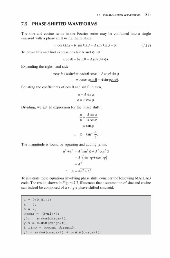
To illustrate these equations involving phase shift, consider the following MATLAB code. The result, shown in Figure 7.7 , illustrates that a summation of sine and cosine can indeed be composed of a single phase - shifted sinusoid.
t = 0:0.01:1; a = 3; b = 2; omega = (2 * pi ) * 4; y1c = a * cos (omega * t); y1s = b * sin (omega * t); % sine + cosine directly y1 = a * cos (omega * t) + b * sin (omega * t);
c07.indd 211c07.indd 211 4/13/2011 5:24:03 PM4/13/2011 5:24:03 PM

212 CHAPTER 7 FREQUENCY ANALYSIS OF SIGNALS
FIGURE 7.7 Converting a sine plus cosine waveform to a sine with phase shift.
Direct—sum of sine and cosine
Indirect—phase–shifted sine
Time
Am
plit
ude
Am
plit
ude
0
0
0
0
0.1
0.1
0.2
0.2
0.3
0.3
0.4
0.4
0.5
0.5
0.6
0.6
0.7
0.7
0.8
0.8
0.9
0.9
1
1
2
2
4
4
–2
–2
–4
–4
7.6 THE FOURIER TRANSFORM
The Fourier transform is closely related to the Fourier series described in the previ-ous section. The fundamental difference is that the requirement to have a periodic signal is now relaxed. The Fourier transform is one of the most fundamental algorithms — if not the fundamental algorithm — in digital signal processing.
7.6.1 Continuous Fourier Transform
The continuous - time Fourier transform allows us to convert a signal x ( t ) in the time domain into its frequency domain counterpart X ( Ω ), where Ω is the true frequency in radians per second. Note that both signals are continuous. The Fourier transform, or (more correctly) the continuous - time/continuous - frequency Fourier transform, is defi ned as
fi gure (1);
plot (t, y1);
% sine with phase shift
phi = atan2 (a, b); A = sqrt (a * a + b * b); y2 = A * sin (omega * t + phi); fi gure (2);
plot (t, y2);
c07.indd 212c07.indd 212 4/13/2011 5:24:03 PM4/13/2011 5:24:03 PM

7.6 THE FOURIER TRANSFORM 213
X x t e dtt( ) ( ) .Ω Ω= −
−∞
∞
∫ j (7.19)
The signal x ( t ) is multiplied by a complex exponential e t−jΩ . This is really just a concise way of representing sine and cosine, since Euler ’ s formula for the complex exponential gives us e t tt− = −j jΩ Ω Ωcos sin .
The functions represented by the e t−jΩ term are sometimes called the basis functions , as depicted in Figure 7.8 . In effect, for a given frequency Ω , the signal x ( t ) is multiplied by the basis functions at that frequency, with the result integrated ( “ added up ” ) to yield an effective “ weighting ” of that frequency component. This is repeated for all frequencies (all values of Ω ) — or at least, all frequencies of inter-est. The result is the spectrum of the time signal. As will be seen later with some examples, the basis functions may be interpreted on the complex plane as shown in Figure 7.9 .
The inverse operation — to go from frequency X ( Ω ) to time x ( t ) — is:
x t X e dt( ) ( ) .=−∞
∞
∫1
2πΩ ΩΩj (7.20)
Note that the difference is in the exponent of the basis function, and the division by 2 π . The latter is related to the use of radian frequency, rather than Hertz (cycles per second).
These two operations — Fourier transform and inverse Fourier transform — are completely reversible. That is, taking any x ( t ), computing its Fourier transform, and then computing the inverse Fourier transform of the result, returns the original signal.
FIGURE 7.8 Sinusoidal basis functions for Fourier analysis: cosine and negative sine.
cosine
–sine
0
0
0
0
π/2
π/2
π
π
3π/2
3π/2
2π
2π
0.5
0.5
1
1
–0.5
–0.5
–1
–1
c07.indd 213c07.indd 213 4/13/2011 5:24:03 PM4/13/2011 5:24:03 PM

214 CHAPTER 7 FREQUENCY ANALYSIS OF SIGNALS
7.6.2 Discrete - Time Fourier Transform
The next stage is to consider a sampled signal. When a signal x ( t ) is sampled at time instants t = nT , resulting in the discrete sampled x ( n ), what happens to the spectrum of the signal? The Fourier transform of a continuous signal is:
X x t e dtt( ) ( ) .Ω Ω= −
−∞
+∞
∫ j
The sampling impulses are impulse or “ delta ” functions δ ( t ) spaced at intervals of T :
r t t nTn
( ) ( ).= −=−∞
+∞
∑δ
The sampled function is the product of the signal at the sampling instants, and the sampling impulses:
x t x t r t
x t t nT
s
n
( ) ( ) ( )
( ) ( ).
=
= −=−∞
+∞
∑ δ (7.21)
FIGURE 7.9 The sine/cosine basis functions may be viewed as a vector on the complex plane.
−
Point on thecomplex plane
sine ( )
cosine
Fourier Transform: Continuous time → Continuous frequency
To summarize the fundamental result from this section, we have:
c07.indd 214c07.indd 214 4/13/2011 5:24:03 PM4/13/2011 5:24:03 PM

7.6 THE FOURIER TRANSFORM 215
Since at the sample instants t = nT , this becomes:
x t x nT t nTs
n
( ) ( ) ( ).= −=−∞
+∞
∑ δ
The Fourier transform of the sampled signal is thus:
X x t e dt
x nT t nT e dt
x n
st
t
n
( ) ( )
( ) ( )
(
Ω Ω
Ω
=
= −
=
−
−∞
+∞
−
=−∞
+∞
−∞
+∞
∫∑∫
j
jδ
TT t nT e dt
x nT e
t
n
n T
n
) ( )
( ) .
δ −
=
−
−∞
+∞
=−∞
+∞
−
=−∞
+∞
∫∑
∑
j
j
Ω
Ω
(7.22)
Note that the delta function has been used here, and the property that:
δ t f t dt f tk k( ) ( ) = ( )−∞
+∞
∫ . (7.23)
Since t = nT (time) and ω = Ω T (frequency), this yields the Fourier transform of a sampled signal as
X x n e n
n
( ) ( ) .ω ω= −
=−∞
+∞
∑ j (7.24)
with
t n Tseconds samplesseconds
sample= × (7.25)
and
ωradians
sample
radians
second
seconds
sample= ×Ω T (7.26)
The (continuous) Fourier transform of a sampled signal as derived above shows that since the complex exponential function is periodic, the spectrum will be periodic — it repeats cyclically, about intervals centered on the sample frequency. Furthermore, the frequency range fs 2 to f s is a mirror image of the range 0 to fs 2. The discrete time Fourier transform (DTFT) may be visualized directly as the multiplication by basis function as illustrated in Figure 7.10 . The difference is that the basis functions of sine and cosine are multiplied by the sample values x ( n ). The frequency ω is, however, free to take on any value (it is not sampled).
Since the frequency spectrum is still continuous, the inverse of the DTFT above is
x n X e dn( ) ( )=−∫
1
2πω ωω
π
πj (7.27)
c07.indd 215c07.indd 215 4/13/2011 5:24:04 PM4/13/2011 5:24:04 PM

216 CHAPTER 7 FREQUENCY ANALYSIS OF SIGNALS
7.6.3 The Discrete Fourier Transform (DFT)
The discrete - time/discrete - frequency Fourier transform — usually known as just the discrete Fourier transform or DFT — is the fi nal stage in the conversion to an all - sampled system. As well as sampling the time waveform, only discrete frequency points are calculated. The DFT equation is:
X k x n e n
n
N
k( ) ( ) ,= −
=
−
∑ j ω
0
1
(7.28)
where
ω π
kk
N
k
=
=
2
frequency of the sinusoidth . (7.29)
FIGURE 7.10 Basis functions for the DFT.
1 cycle
1.5 cycles
2 cycles
10 cycles
0 π/2 π 3π/2 2π
0 π/2 π 3π/2 2π
0 π/2 π 3π/2 2π
0 π/2 π 3π/2 2π
Discrete Time Fourier Transform: Sampled time → Continuous frequency
To summarize the fundamental result from this section, we have
c07.indd 216c07.indd 216 4/13/2011 5:24:04 PM4/13/2011 5:24:04 PM

7.6 THE FOURIER TRANSFORM 217
The discrete basis functions are now at points on the complex plane, or 1⋅ −e n kj ω , as illustrated in Figure 7.11 . This gives rise to the result that the DFT is now cyclic, and in effect, only the frequencies up to ω = π are of interest. A consequence of the frequency points going all the way around the unit circle is that when we take the DFT, the upper half of the resulting components are a mirror image of the lower half. This will be illustrated later using some examples.
Recall that the z transform was defi ned in Section 5.4 as the expansion:
F z f z f z f z
f n z n
n
( )
( ) .
= ( ) + ( ) + ( ) +
=
− −
−
=
∞
∑0 1 20 1 2
0
�
(7.30)
Comparing this with the defi nition of the DFT in Equation 7.28 , it may be seen that the DFT is really a special case of the z transform with the substitution
z e k= jω . (7.31)
That is, the DFT is the z transform evaluated at the discrete points around the unit circle defi ned by the frequency ω . Understanding this result is crucial to understand-ing the applicability and use of Fourier transforms in sampled - data systems.
As in previous cases, there is an inverse operation to convert from the fre-quency domain back to the time domain samples. In this case, it is the inverse DFT to convert frequency samples X ( k ) back to time samples x ( n ), and is given by:
x nN
X k e n
k
N
k( ) ( ) .==
−
∑1
0
1j ω (7.32)
FIGURE 7.11 DFT basis functions as points on the unit circle. This is described by a complex exponential e kjω .
ωk = 2πkN
c07.indd 217c07.indd 217 4/13/2011 5:24:04 PM4/13/2011 5:24:04 PM

218 CHAPTER 7 FREQUENCY ANALYSIS OF SIGNALS
Note that the forward and inverse operations are quite similar: the difference is in the sign of the exponent and the division by N .
To summarize the fundamental result from this section, we have:
Discrete Fourier Transform: Sampled time → Sampled frequency
7.6.4 The Fourier Series and the DFT
Clearly, the Fourier series and Fourier transform are related, and we now wish to explore this idea. Recall that the Fourier series for a continuous function x ( t ) was shown in Section 7.3 to be:
x t a
a t a t a t
b t b t bo o o
o o
( )
cos cos cos
sin sin
= ++ + ++ +
0
1 2 3
1 2
2 3
2
Ω Ω ΩΩ Ω
�
33
0 0 0
1
3sin
cos sin
Ω
Ω Ω
o
k k
k
t
a a k t b k t
+
= + +( )=
∞
∑� (7.33)
with coeffi cients a k and b k :
a x t dt00
1= ∫ττ
( ) (7.34)
a x t k t dtk o= ∫20τ
τ( )cos Ω (7.35)
b x t k t dtk o= ∫20τ
τ( )sin Ω . (7.36)
As before, the integration limits could equally be −τ 2 to + τ 2. Also, the complex form is:
x t c ekk t
k
k
o( ) .==−∞
=+∞
∑ j Ω (7.37)
with coeffi cients:
c x t e dtkk to= −∫1
0τ
τ( ) .j Ω (7.38)
The discrete Fourier transform was shown to be
c07.indd 218c07.indd 218 4/13/2011 5:24:04 PM4/13/2011 5:24:04 PM

7.6 THE FOURIER TRANSFORM 219
X k x n e n
n
N
k( ) ( ) ,= −
=
−
∑ j ω
0
1
(7.39)
with ωπ
kk
N= 2
, which is just the frequency of the k th sinusoid.
Comparing the c k terms in the Fourier series equation with the X ( k ) terms in the DFT equation, it may be seen that they are essentially the same except for divi-sion by the total time in the Fourier series. The DFT is really a discretized version of the Fourier series, with N samples spaced dt apart. In the limit as T → 0, the DFT becomes a continuous Fourier transform.
By expanding the sine - cosine Fourier series equations and the complex - number form, it may be observed that there is a correspondence between the terms:
a c
a e c
b m ck k
k k
0 0
2
2
== + { }= − { }R
I .
The division by τ (total waveform period) in the Fourier series equations becomes division by N in the Fourier transform equations. So, the Fourier transform outputs may be interpreted as scaled Fourier series coeffi cients:
aN
X
aN
e X k
bN
m X k
k
k
01
0
2
2
=
= + { }
= − { }
( )
( )
( ) .
R
I
Another way to see the reason for the factor of two is to consider the “ folding ” from 0 to N 2 1− and N 2 to N − 1. Half the “ energy ” of the terms is in the lower half of the output, the other half is in the upper half of the output. An easy solution is to take the fi rst half of the transform coeffi cients and to double them. The fi rst coef-fi cient X (0) is not doubled, as its counterpart is the very fi rst coeffi cient after the output sequence, or the N th coeffi cient. This will be illustrated shortly with some examples.
Note that it is important not to misunderstand the relationship between the Fourier series and the DFT. The Fourier series builds upon harmonics (integer mul-tiples) of a fundamental frequency. The DFT dispenses with the integer harmonic constraint, and the limit of frequency resolution is dictated by the number of sample points.
7.6.5 Coding the DFT Equations
Some examples will now be given on the use and behavior of the DFT. First, we need a MATLAB implementation of the DFT equations:
c07.indd 219c07.indd 219 4/13/2011 5:24:04 PM4/13/2011 5:24:04 PM

220 CHAPTER 7 FREQUENCY ANALYSIS OF SIGNALS
For the sake of effi ciency, the loops may also be coded in MATLAB using vectorized operations as follows (vectorizing code was covered in Chapter 2 — the numerical result does not change, but the calculation time is reduced).
% MATLAB vectorized version
function [XX] = dftv(x) x = x(:); N = length (x); XX = zeros (N, 1); n = [0:N − 1] ’ ; for k = 0:N − 1 wk = 2 * pi * k/N; XX(k + 1) = sum (x. * exp ( − j * n * wk)); end
7.6.6 DFT Implementation and Use: Examples in MATLAB
So, what about the relationship between the DFT component index and the actual frequency? The DFT spans the relative frequency range from 0 to 2 π radians per sample, which is equivalent to a real frequency range of 0 – f s . There are N + 1 components in this range, hence the spacing in frequency of each is f Ns . The “ zeroth ” component is the zero - frequency or “ average ” value. The fi rst component is one N th of the way to f s . This is reasonable, since a waveform of exactly one sinusoidal cycle over N components has a frequency of one N th of f s .
The scaling in time and frequency of the DFT components will now be illus-trated by way of some MATLAB examples. The following examples use the built - in MATLAB function fft (), or fast Fourier transform. The details of this algorithm will be explained in Section 7.12 , but for now it is suffi cient to know that it is identi-cal to the DFT, provided the number of input samples is a power of 2 .
% function [ XX ] = dft ( x ) %
% compute the DFT directly
% x = column vector of time samples (real) % XX = column vector of complex – valued % frequency – domain samples
function [XX] = dft(x) N = length (x); XX = zeros (N, 1); for k = 0:N − 1 wk = 2 * pi * k/N; for n = 0:N − 1 XX(k + 1) = XX(k + 1) + x(n + 1) * exp ( − j * n * wk); end
end
c07.indd 220c07.indd 220 4/13/2011 5:24:04 PM4/13/2011 5:24:04 PM

7.6 THE FOURIER TRANSFORM 221
To begin with, recall some basic sampling terminology and equations from Chapter 5 . A sinusoidal waveform was mathematically described as:
x t A t( ) sin .= Ω
Sampled at t = nT , this became the samples x ( n ) at instant n :
x n A nT
A n T
( ) sin
sin .
==
ΩΩ
Defi ning ω as
ω = ΩT ,
we have:
x n A n( ) sin ,= ω (7.40)
where ω is measured in radians per sample. For one complete cycle of the waveform in N samples, the corresponding angle
ω swept out in one sample period will be just ω π= 2 N .
7.6.6.1 DFT Example 1: Sine Waveform To begin with a simple signal, we use MATLAB to generate one cycle of a sinusoidal waveform, and analyze it using the DFT. Since there is only one sinusoidal component, the resulting DFT array X ( k ) should have only one component. Sixty - four samples are used for this example:
N = 64; n = 0:N − 1; w = 2 * pi /N; x = sin (n * w); stem (x);
XX = fft (x);
The zero - frequency or DC coeffi cient is zero as expected. The value is not precisely zero, because normal rounding errors apply:
XX(1)/N
ans = 8.8524e − 018
c07.indd 221c07.indd 221 4/13/2011 5:24:04 PM4/13/2011 5:24:04 PM

222 CHAPTER 7 FREQUENCY ANALYSIS OF SIGNALS
Note 2 that coeffi cient number 1 (at index 2) is −1j. This may be interpreted in terms of the basis functions, since real numbers correspond to cosine components, and imaginary correspond to negative sine. So a positive sine coeffi cient equates to a negative imaginary value. Coeffi cients 64, 63, 62 are the complex conjugates of the samples at indexes 2, 3, and 4.
m = abs (XX); p = angle (XX); iz = fi nd ( abs (m < 1)); p(iz) = zeros ( size (iz)); subplot (2, 1, 1); stem (m);
subplot (2, 1, 2); stem (p);
XX(N − 2:N)/N * 2 ans = 0.0 + 0.0i 0.0 + 0.0i 0.0 + 1.0i
This is due to the fact that the frequency ω k goes all the way around the unit circle, as shown previously. The range from 0 to π corresponds to frequencies 0 to fs 2 (half the sampling rate). The range from π to 2 π is a “ mirror image ” of the lower frequency components. Plotting the DFT magnitudes and phases is accom-plished with:
Note that the phase angle of components with a small magnitude was set to zero for clarity in lines 3 and 4.
7.6.6.2 DFT Example 2: Waveform with a Constant Offset Again, we generate a 64 - sample sine waveform, but this time with a zero - frequency or DC component. The code to test this is shown below, along with the results for the zero - frequency (DC) component, and the fi rst frequency component. These have values of 5 and −1j, as expected.
2 Remember that MATLAB uses i rather than j to denote the complex quantity j = −1.
XX(2:4)/N * 2
ans = 0.0 − 1.0i 0.0 − 0.0i 0.0 − 0.0i
The scaled coeffi cients 1, 2, 3 are:
c07.indd 222c07.indd 222 4/13/2011 5:24:04 PM4/13/2011 5:24:04 PM

7.6 THE FOURIER TRANSFORM 223
Note that, as always, index 1 in the vector is the subscripted component X (0). This result is as we would expect — we have a zero - frequency or DC component, together with a −1j for the sinusoidal component.
7.6.6.3 DFT Example 3: Cosine Waveform The previous example used a sine component. In this example, we generate a 64 - sample cosine waveform with a DC component:
N = 64; n = 0:N − 1; w = 2 * pi /N; x = cos (n * w) + 5; stem (x);
XX = fft (x); XX(1)/N
ans = 5
XX(2:4)/N * 2
ans = 1.0 − 0.0i 0 0.0 + 0.0i
N = 64; n = 0:N − 1; w = 2 * pi /N; x = sin (n * w) + 5; stem (x);
XX = fft (x); % DC component
XX(1)/N
ans = 5
% fi rst two frequency components
XX(2:4)/N * 2
ans = 0.0 − 1.0i 0 0.0 − 0.0i
As with the earlier discussion on basis functions, the value of 1 0+ j indicates the presence of a cosine component. The magnitude of the value also tells us the magnitude of this component.
7.6.6.4 DFT Example 4: Waveform with Two Components This example illustrates the process of resolving the underlying components of a waveform. We take a 256 - sample waveform with two additive components, and examine the DFT:
c07.indd 223c07.indd 223 4/13/2011 5:24:04 PM4/13/2011 5:24:04 PM

224 CHAPTER 7 FREQUENCY ANALYSIS OF SIGNALS
N = 256; x = zeros (N, 1); x(1) = 1; for n = 2:N x(n) = − 1 * x(n − 1); end
f = fft (x); stem ( abs (f));
[v i] = max ( abs (f)) v = 256
i = 129
N = 256; n = 0:N − 1; w = 2 * pi /N; x = 7 * cos (3 * n * w) + 13 * sin (6 * n * w); plot (x);
XX = fft (x); XX(1)/N
ans = − 2.47e − 016 XX(2:10)/N * 2
ans = Columns 1 through 4
0.0 + 0.0i 0.0 + 0.0i 7.0 − 0.0i 0.0 + 0.0i Columns 5 through 8
0.0 + 0.0i 0.0 − 13.0i 0.0 − 0.0i 0.0 − 0.0i Column 9
0.0 − 0.0i
Note that the DFT is able to resolve the frequency components present. The frequency resolution may be seen from the fact that there are N points spanning up to f s , and so the resolution of each component is f Ns .
7.6.6.5 DFT Example 5: Limits in Frequency To look more closely at the frequency scaling of the DFT, we generate an alternating sequence of samples having values + 1, − 1, + 1, − 1, . . . . This is effectively a waveform at half the sampling frequency.
c07.indd 224c07.indd 224 4/13/2011 5:24:04 PM4/13/2011 5:24:04 PM

7.6 THE FOURIER TRANSFORM 225
In MATLAB, vector indices for a 256 - point vector are numbered from 1 to 256, as illustrated in Figure 7.12 . Starting at 0, this corresponds to the range 0 – 255. Component number 129 contains the only frequency component. Now, the fi rst half of the frequency components are numbered 1 – 128, so component 129 is the fi rst component in the second half — and this corresponds to the input frequency, namely f fs= 2. The frequency f = f s is, in fact, the fi rst component after the last, or the 257th component (not generated here). Thus the frequency interval is f Ns . The fi rst component, number 1, is actually the zero - frequency or “ DC ” component. Hence, it is easier to imagine the indices from 0 to N − 1. Using the MATLAB indices of k = 1, … , N , we have:
The “ true ” frequency of component 1 is 0 0× =f
Ns .
The true frequency of component 2 is 1× f
Ns .
The true frequency of component 3 is 2 × f
Ns .
The true frequency of component k is ( )kf
Ns− ×1 .
In the example,
The true frequency of component 257 (not generated) is 256256
× =ffss.
The true frequency of component 129 is 128256 2
× =f fs s .
Figure 7.12 illustrates these concepts.
FIGURE 7.12 Illustrating DFT components for an N = 256 transform. MATLAB indices start at 1, whereas the DFT equations assume zero - based indexing. The set of upper half returned values is a mirror image of the lower half, with the “ pivot point ” being the fs 2sample.
1 2
0 1
Δ
Δ = f s
N
0
128 129
Lower half Upper half
127 128
f s
2 f s
256 257
255 256
c07.indd 225c07.indd 225 4/13/2011 5:24:04 PM4/13/2011 5:24:04 PM

226 CHAPTER 7 FREQUENCY ANALYSIS OF SIGNALS
7.6.6.6 DFT Example 6: Amplitude and Frequency If we now alter both the amplitude and frequency of the input signal, the DFT result ought to refl ect this. The waveform with fi ve cycles of a simple sinusoidal waveform of amplitude 4 is cal-culated as:
N
n N
Nx n n
== … −
=
=
64
0 1 1
2
4 5
, , ,
( ) sin( ).
ω π
ω
(7.41)
The waveform and its DFT are shown in Figure 7.13 . Note in particular:
1. The index of the lower frequency peak and its corresponding frequency.
2. The location of the higher frequency peak (the mirror image).
3. The height of the frequency peaks.
7.6.6.7 DFT Example 7: Resolving Additive Waveforms Extending the pre-vious example, we now take the DFT of two additive sinusoidal waveforms, each with a different amplitude and frequency:
FIGURE 7.13 DFT example: 5 cycles of amplitude 4 in the time and frequency domains.
0 8 16 24 32 40 48 56 63−10
−6
−2
2
6
10
Sampled waveform 4sin(5nω)
0 8 16 24 32 40 48 56 630
32
64
96
128
FFT of sampled waveform
c07.indd 226c07.indd 226 4/13/2011 5:24:05 PM4/13/2011 5:24:05 PM
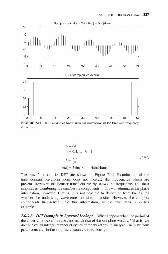
7.6 THE FOURIER TRANSFORM 227
N
n N
Nx n n n
== −
=
= +
64
0 1 1
2
2 1 4 4
, , ,
( ) sin( ) sin( ).
…
ω π
ω ω
(7.42)
The waveform and its DFT are shown in Figure 7.14 . Examination of the time domain waveform alone does not indicate the frequencies which are present. However, the Fourier transform clearly shows the frequencies and their amplitudes. Combining the sine/cosine components in this way eliminates the phase information, however. That is, it is not possible to determine from the fi gures whether the underlying waveforms are sine or cosine. However, the complex components themselves yield this information, as we have seen in earlier examples.
7.6.6.8 DFT Example 8: Spectral Leakage What happens when the period of the underlying waveform does not match that of the sampling window? That is, we do not have an integral number of cycles of the waveform to analyze. The waveform parameters are similar to those encountered previously:
FIGURE 7.14 DFT example: two sinusoidal waveforms in the time and frequency domains.
0 8 16 24 32 40 48 56 63−10
−6
−2
2
6
10
Sampled waveform 2sin(1nω) + 4sin(4nω)
0 8 16 24 32 40 48 56 630
32
64
96
128
FFT of sampled waveform
c07.indd 227c07.indd 227 4/13/2011 5:24:05 PM4/13/2011 5:24:05 PM

228 CHAPTER 7 FREQUENCY ANALYSIS OF SIGNALS
N
n N
wN
x n n
== … −
=
( ) = ( )
64
0 1 1
2
4 2 5
, , ,
sin . .
π
ω
(7.43)
The sampled waveform is shown in Figure 7.15 — note that there are 2 12 cycles in
the analysis window, as expected. The product of some of the basis - vector wave-forms and the input waveform will be nonzero, resulting in some nonzero sine and cosine components around the frequency of the input.
The DFT of this waveform is shown in Figure 7.15 . Note the “ spillover ” in the frequency components, due to the fact that a noninteger number of cycles was taken for analysis. This is a fundamental problem in applying the DFT, and motivates the question: if we do not know in advance the expected frequencies contained in the waveform, how long do we need to sample for, in order for this problem not to occur? We have already determined that the resolution in the DFT is governed by the number of samples in the time domain, but now we have the further problem as illustrated in this example. To answer this question fully requires some further
FIGURE 7.15 DFT example: a nonintegral number of cycles of a sinusoidal waveform. In this case, the DFT does not resolve the waveform into a single component as might be expected.
0 8 16 24 32 40 48 56 63−10
−6
−2
2
6
10
Sampled waveform 4sin(2.5nω)
0 8 16 24 32 40 48 56 630
32
64
96
128
FFT of sampled waveform
c07.indd 228c07.indd 228 4/13/2011 5:24:05 PM4/13/2011 5:24:05 PM

7.6 THE FOURIER TRANSFORM 229
analysis and consideration of the “ sampling window ” in Section 7.9 . But clearly, we must be careful in interpreting the results produced by the DFT.
7.6.6.9 DFT Example 9: Additive Noise Now consider the case of nonperi-odic noise added to sinusoidal components. This type of scenario is typical of com-munications and speech processing systems, where one or more periodic signals have noise superimposed.
N
n N
wN
x n n n v n
== −
=
( ) = ( ) + ( ) + ( )
64
0 1 1
2
2 1 4 4
, , ,
sin sin .
…π
ω ω α
(7.44)
Here, v ( n ) represents the additive noise signal, with the amount controlled by param-eter α . The waveform and its DFT are shown in Figure 7.16 . From these plots, it is evident that the periodic components still feature strongly in the frequency domain. The DFT step makes the underlying components clearer than in the time domain waveform.
FIGURE 7.16 DFT example: a complex sinusoidal waveform with additive noise in the time and frequency domains.
0 8 16 24 32 40 48 56 63−10
−6
−2
2
6
10
Sampled waveform 2sin(1nω) + 4sin(4nω) + α v(n)
0 8 16 24 32 40 48 56 630
32
64
96
128
FFT of sampled waveform
c07.indd 229c07.indd 229 4/13/2011 5:24:05 PM4/13/2011 5:24:05 PM

230 CHAPTER 7 FREQUENCY ANALYSIS OF SIGNALS
7.6.6.10 DFT Example 10: Noisy Waveform Restoration This example con-siders a waveform with additive noise. Thresholding is done in the frequency domain (note the MATLAB vectorized method of doing this). The real part of the inverse FFT, ifft (), is taken, because although the imaginary part should be zero in the time domain, it may have a very small imaginary component due to rounding and the effects of fi nite numerical precision.
The result, shown in Figure 7.17 , shows that the operation of taking the fre-quency components, thresholding, and taking the inverse DFT is able to restore the signal. In practice, however, taking an arbitrary threshold may not be desirable, since the actual signal as presented may vary from the test signal shown. Thus, a more advanced approach may be warranted — for example, if more than one frame of data signal is available, we may be able to average over multiple frames of signal rather than base the results on one single frame.
FIGURE 7.17 DFT and noise removal.
0 8 16 24 32 40 48 56 63−10
−6
−2
2
6
10
Sampled waveform 2sin(1nω) + 4sin(4nω) + α v(n)
0 8 16 24 32 40 48 56 63−10
−6
−2
2
6
10IFFT of thresholded FFT
N = 64; n = 0:N − 1; w = 2 * pi /N; x = 2 * sin (1 * n * w) + 4 * sin (4 * n * w) + 1 * randn (1,N);
c07.indd 230c07.indd 230 4/13/2011 5:24:06 PM4/13/2011 5:24:06 PM

7.7 ALIASING IN DISCRETE-TIME SAMPLING 231
7.7 ALIASING IN DISCRETE - TIME SAMPLING
The problem of choosing the sampling rate for a given signal was discussed in Section 3.8 . The Fourier transform now provides us with a more analytical way to look this problem, and the related problem of aliasing when we sample a signal.
In Section 3.5 , sampling was introduced as a multiplication of the continuous - time analog signal with the sampling pulses (the “ railing ” function). The Fourier series expansion of the sampling impulses of frequency Ω s can be shown to be:
r t
T Tt
Tt
Tt
Tt t
s s s
s s
( ) = + + + +
= + +
1 2 22
23
2 1
22
cos cos cos
cos cos
Ω Ω Ω
Ω Ω
�
++ +⎛⎝⎜
⎞⎠⎟cos .3Ωst �
(7.45)
We know that sampling is equivalent to multiplying the signal x ( t ) by the railing function r ( t ) to obtain the sampled signal x s ( t ). To simplify notation, we replace the cosine function with its complex exponential equivalent:
r tT
t t t
Tt
s s s
s
( ) = + + + +⎛⎝⎜
⎞⎠⎟
= + +
2 1
22 3
11 2 2 2
cos cos cos
cos cos
Ω Ω Ω
Ω
�
ΩΩ Ω
Ω Ω Ω Ω
s s
t t t t
t t
Te e e e e es s s s
+ +( )
= + +( ) + +( ) +− −
2 3
1 0 2 2 3
cos �
j j j j j jj j
j
Ω Ω
Ω
s s
s
t t
k t
k
e
Te
+( ) +( )
=
−
=−∞
+∞
∑
3
1
�
.
(7.46)
The sampled signal is x s ( t ) = x ( t ) r ( t ), and we need to determine the effect of the sampling in the frequency domain. As before, the Fourier transform of the continu-ous signal is:
X x t e dttΩ Ω( ) = ( ) −
−∞
+∞
∫ j .
Using these results, we can derive the Fourier transform of the sampled signal as follows.
subplot (2,1,1);
plot (n,x);
f = fft (x); i = fi nd ( abs (f) < 40); f(i) = zeros ( size (i)); xr = ifft (f); subplot (2,1,2);
plot (n,xr);
c07.indd 231c07.indd 231 4/13/2011 5:24:06 PM4/13/2011 5:24:06 PM

232 CHAPTER 7 FREQUENCY ANALYSIS OF SIGNALS
X x t e dt
x t r t e dt
x tT
e
s st
t
k ts
Ω Ω
Ω
Ω
( ) = ( )
= ( ) ( )
= ( )
−
−∞
+∞
−
−∞
+∞
−∞
∫∫
j
j
1++∞
( )
−
−∞
+∞
−
−∞
+∞
∑∫
∫
⎛⎝⎜
⎞⎠⎟
= ( )
r t
t
k t t
e dt
Tx t e e dts
� ��� ���
j
j j
Ω
Ω Ω1 ⎛⎛⎝
⎞⎠
= ( )⎛⎝
⎞⎠
= ( )
=−∞
+∞
− −( )−∞
+∞
=−∞
+∞
−
∑
∫∑k
k t
kT
x t e dt
Tx t e
s1
1
j
j
Ω Ω
ΩΩ Ω+( )−∞
+∞
=
+∞
∫∑⎛⎝
⎞⎠
k t
k
s dt0
.
(7.47)
The integral (in brackets) is X ( Ω ± k Ω s ), which is the spectrum X ( Ω ) shifted by ± k Ω s . So the spectrum of the sampled waveform is:
XT
X ks s
k
Ω Ω Ω( ) = ±( )=
∞
∑1
0
(7.48)
The above equation demonstrates why aliasing occurs, and may be expressed in words as follows:
The spectrum of the signal X ( Ω ) is “ mirrored ” at ± ± ±Ω Ω Ωs s s, , ,2 3 …
We can understand this further by returning to the fi rst introduction of aliasing in Chapter 3 . Figure 7.18 shows the problem in the time domain, and now we are able to interpret this in terms of frequency. Referring to Figure 7.18 , we fi rst sample below the input frequency. Clearly, we cannot expect to capture the information about the waveform if we sample at a frequency lower than the waveform itself, so this is just a hypothetical case. The waveform appears to have a frequency of | f − f s | = |4 − 3| = 1 Hz. Next, we sample at 5 Hz, which is a little above the wave-form frequency. This is still inadequate, as shown. The frequency is effectively “ folded ” down to | f − f s | = |4 − 5| = 1 Hz. Finally, we sample at greater than twice the frequency ( f s > 2 f , or 10 Hz > 2 × 4 Hz). The sampled waveform does not produce a lower “ folded - down ” frequency.
Figure 7.19 illustrates this approach, from the frequency domain perspective. It shows that as the sampling frequency is reduced relative to the frequency spectrum of the signal being sampled, a point will be reached where the baseband spectrum and the “ ghost ” spectrum overlap. Once this occurs, the signal cannot be inverted back into the time domain without aliasing occurring.
c07.indd 232c07.indd 232 4/13/2011 5:24:06 PM4/13/2011 5:24:06 PM

7.8 THE FFT AS A SAMPLE INTERPOLATOR 233
FIGURE 7.18 How aliasing arises in the time domain. A 4 - Hz sinewave is sampled, so the Nyquist rate is 8 Hz, and we should sample above that rate.
0 0.2 0.4 0.6 0.8 1 1.2 1.4 1.6 1.8 2
Aliasing in sampling: f = 4 Hz, fs = 3 Hz
Time (s)
0 0.2 0.4 0.6 0.8 1 1.2 1.4 1.6 1.8 2
Aliasing in sampling: f = 4 Hz, fs = 5 Hz
Time (s)
0 0.2 0.4 0.6 0.8 1 1.2 1.4 1.6 1.8 2
No aliasing in sampling: f = 4 Hz, f s = 10 Hz
Time (s)
7.8 THE FFT AS A SAMPLE INTERPOLATOR
As an interesting insight, consider the generation of missing samples in a sequence. This is related to the problem of interpolating the signal value between known samples, as introduced in Section 3.9.1 .
c07.indd 233c07.indd 233 4/13/2011 5:24:06 PM4/13/2011 5:24:06 PM

234 CHAPTER 7 FREQUENCY ANALYSIS OF SIGNALS
To begin with, consider Figure 7.20 . This fi gure shows zeros inserted into the sample sequence between every known sample, so as to generate a new sample sequence. This is about as simple an operation as we could imagine, and effectively doubles the sample rate (even though the new zero - valued samples obviously bear no relation to the true samples).
But what is the effect in the frequency domain? If we take the zero - inserted sequence and examine its FFT, we see, as in Figure 7.21 , that spurious components have been introduced. Considering the frequency - domain interpretation, we may say that these correspond to the high - frequency components introduced by the zero values at every second sample.
If we then remove these high - frequency components and take the inverse FFT, we see that the original signal has been “ smoothed ” out, or interpolated, as shown in Figure 7.22 . The following MATLAB code shows how to use the reshape () function to perform zero - sample interpolation:
FIGURE 7.19 Sampling rate and “ folding frequency ” . The true spectrum is that shown over the range 0 to fs 2. The secondary spectral images are artifacts of the sampling process. If the spectra overlap, aliasing occurs.
Adequate sample rate compared with bandwidth
Marginal sample rate compared with bandwidth
Inadequate sample rate compared with bandwidth
0
0
+ f s / 2
+ f s / 2
− f s / 2
− f s / 2
+ f s
+ f s
− f s
− f s
c07.indd 234c07.indd 234 4/13/2011 5:24:06 PM4/13/2011 5:24:06 PM
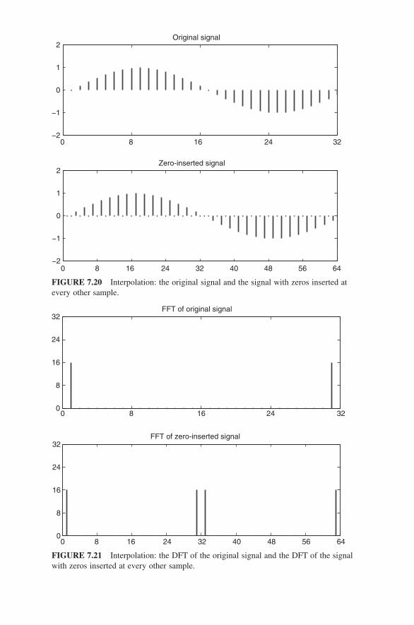
FIGURE 7.20 Interpolation: the original signal and the signal with zeros inserted at every other sample.
0 8 16 24 32−2
−1
0
1
2Original signal
0 8 16 24 32 40 48 56 64−2
−1
0
1
2Zero-inserted signal
FIGURE 7.21 Interpolation: the DFT of the original signal and the DFT of the signal with zeros inserted at every other sample.
0 8 16 24 320
8
16
24
32FFT of original signal
0 8 16 24 32 40 48 56 640
8
16
24
32FFT of zero-inserted signal
c07.indd 235c07.indd 235 4/13/2011 5:24:06 PM4/13/2011 5:24:06 PM

236 CHAPTER 7 FREQUENCY ANALYSIS OF SIGNALS
FIGURE 7.22 Interpolation after removing the high - frequency components in the zero - inserted sequence.
0 8 16 24 32−2
−1
0
1
2Original signal
0 8 16 24 32 40 48 56 64−2
−1
0
1
2Interpolated signal
7.9 SAMPLING A SIGNAL OVER A FINITE TIME WINDOW
Considering the preceding discussion, two problems are apparent with discrete - data spectrum estimation:
1. The sampling rate limits the maximum frequency we can observe, and may introduce aliasing if proper fi ltering is not present at the input.
N = 32; n = 0:N − 1; w = 2 * pi /N; x = sin (n * w); f = fft (x); xi = [x; zeros (1, N)]; xi = reshape (xi, 2 * N, 1); fi = fft (xi); fi(32) = 0; fi(34) = 0; xr = 2 * real ( ifft (fi));
c07.indd 236c07.indd 236 4/13/2011 5:24:06 PM4/13/2011 5:24:06 PM

7.9 SAMPLING A SIGNAL OVER A FINITE TIME WINDOW 237
2. We can only sample data over a fi nite time record. The continuous - time Fourier equations used infi nite time limits, which is of course impractical.
Furthermore, what happens if the frequency content of the signal changes over the sampling time? We will examine this related issue in Section 7.10 . So the question we must examine theoretically is this: since we can only sample for a fi nite amount of time, what is the effect on the spectrum? As we have seen, the Fourier Transform of a continuous signal is
X x t e dttΩ Ω( ) = ( ) −
−∞
+∞
∫ j .
If this is truncated to a fi nite length (because we sample the waveform for a fi nite time), say ± τ , then the transform becomes
X x t e dttΩ Ω( ) = ( ) −
−
+
∫ j
τ
τ. (7.49)
Suppose x ( t ) is a sine wave of frequency Ω o radians/second:
x t to( ) = sin .Ω (7.50)
In exponential form,
x t e eo ot t( ) = −( )−1
2jj jΩ Ω . (7.51)
The windowed spectrum becomes:
X e e e dto ot t tΩ Ω Ω Ω( ) = −( )− −
−
+
∫ 1
2jj j j
τ
τ. (7.52)
Performing the integration, the magnitude becomes a pair of sinc functions centered at ± Ω o ,
X o oΩ Ω Ω Ω Ω( ) = −( ) + +( )τ τ τ τsinc sinc , (7.53)
where the “ sinc ” function is as previously defi ned, of the form 3
sinc .θ θθ
= sin (7.54)
Noting that the sinc function is a sin θ component multiplied by a 1/ θ component, we can deduce that the shape is sinusoidal in form, multiplied by an envelope that decays as 1/ θ . Here, the θ is actually Ω τ , with Ω offset by the fi xed frequency Ω o . Thus, the resulting spectrum is a pair of sinc functions, centered at ± Ω o . The sinc function sinθ θ( ) has zero crossings at ± π , ± 2 π , … , and thus the zero crossings Ω c of the sinc function are at:
Ω Ωo c k±( ) = ±τ π (7.55)
∴ = ± ±Ω Ωc okπτ
(7.56)
3 Some texts defi ne sinc t t t= ( )sinπ π .
c07.indd 237c07.indd 237 4/13/2011 5:24:06 PM4/13/2011 5:24:06 PM

238 CHAPTER 7 FREQUENCY ANALYSIS OF SIGNALS
That is, as the length of the window increases and τ → ∞ , the zero crossings tend to be closer and closer to the “ true ” frequency. In other words, the sinc function tends to an impulse at the frequency of the input sine wave. A rectangular window over the time interval − 2 ≤ t ≤ 2 is shown in Figure 7.23 . Note that the window is “ implicit, ” in that we are taking only a fi xed number of samples.
The type of spectral estimate resulting from a rectangular window is shown in the successive plots in Figures 7.24 and 7.25 . Each point in the lower panel is one point on the spectrum. This is derived by multiplying the input waveform by each of the sine and cosine basis functions, adding or integrating over the entire time period, and taking the magnitude of the resulting complex number. Figure 7.24 shows the situation when the analysis frequency is relatively low, and Figure 7.25 shows the situation when the analysis frequency is just higher than the input frequency.
This may also be understood by the fundamental theorem of convolution: multiplication in the time domain equals convolution in the frequency domain. Thus, multiplication of a signal which is infi nite in extent, by a fi nite rectangular window in the time domain, results in a spectrum which is the convolution of the true spec-trum (an impulse in the case of a sine wave) with the frequency response of the rectangular window. The latter was shown to be a sinc function. Thus, the true fre-quency estimates are “ smeared ” by the sinc function.
FIGURE 7.23 Windowing: an infi nite sine wave (upper) is multiplied by a rectangular window, to yield the windowed waveform (bottom). Note that if we do sample over a fi nite time limit, we have effectively windowed the waveform. Ambiguity arises because our window (and hence the sampling) is not synchronized to the underlying signal.
0
0
0
1
1
1
–1
–1
–1
0
0
0
1
1
1
2
2
2
3
3
3
4
4
4
–1
–1
–1
–2
–2
–2
–3
–3
–3
–4
–4
–4
c07.indd 238c07.indd 238 4/13/2011 5:24:06 PM4/13/2011 5:24:06 PM

FIGURE 7.24 The effect of a window on the spectrum. The upper panel shows the signal to be analyzed using the sine and cosine basis functions (middle). The resulting spectrum is built up in the lower plot; at this time instant, there is little correlation and so the amplitude is small.
Original signal to analyze over finite time window
Time
Complex exponential = sine & cosine waves
Time
Resulting sum-of-product (spectrum)
Frequency
Current frequency point
FIGURE 7.25 As the analysis frequency is increased, the signals align to a greater degree and so the spectral magnitude is larger. Clearly, the resultant spectrum is not a single value at the input frequency, as might be expected, but is spread over nearby frequencies. This gives rise to ambiguity in determining the true frequency content of the input signal.
Original signal to analyze over finite time window
Time
Complex exponential = sine & cosine waves
Time
Resulting sum-of-product (spectrum)
Frequency
Current frequency point
c07.indd 239c07.indd 239 4/13/2011 5:24:06 PM4/13/2011 5:24:06 PM

240 CHAPTER 7 FREQUENCY ANALYSIS OF SIGNALS
FIGURE 7.26 The evolution of a “ chirp ” signal, whose frequency increases over time. The darker sections correspond to greater energy in the signal at a particular time and frequency. On the left is a portion of the time domain waveform. On the right is the time - frequency plot.
0 0.05 0.1 0.15 0.2 0.25
−0.8
−0.6
−0.4
−0.2
0
0.2
0.4
0.6
0.8
Chirp waveform
Time (s)
Am
plit
ude
Fre
quency H
z
Time (s)
Chirp time-frequency
0 0.2 0.4 0.6 0.8 1
1,000
900
800
700
600
500
400
300
200
100
Fs = 8000; dt = 1/Fs; N = 2 ̂ 13; % ensure a power of 2 for FFT t = 0:dt:(N − 1) * dt; f = 400; fi = (1: length (t))/ length (t) * f; y = sin (2 * pi * t. * fi ); plot (y(1:2000));
sound (y, Fs);
7.10 TIME - FREQUENCY DISTRIBUTIONS
In many applications, we are interested in not simply the spectral content of a signal, but how that spectral content evolves over time. Probably the best example is the speech signal — the frequency content of speech obviously changes over time. For a simpler real - world example, think of a vehicle with a siren moving toward an observer. Because of the Doppler effect, the frequency increases as the vehicle moves toward the observer, and decreases as it moves away.
An obvious way to approach this problem is to segment the samples into smaller frames or blocks. The Fourier analysis techniques can then be applied to each frame in turn. This is termed a spectrogram .
The following generates a “ chirp ” signal, which is one whose frequency increases over time:
Plotting the FFT magnitude shows only the average power in the signal over all time. Using the spectrogram, we obtain a time - frequency plot as shown in Figure 7.26 . This shows higher energy with a darker color.
c07.indd 240c07.indd 240 4/13/2011 5:24:06 PM4/13/2011 5:24:06 PM

7.11 BUFFERING AND WINDOWING 241
As an illustration of a more complicated signal, Figure 7.27 shows the spec-trograms of a speech utterance, the sentence “ today is Tuesday. ” To attain greater accuracy in the frequency domain, a longer sample record is required. However, this means less accuracy in the time domain, because the frequency content of the signal changes relatively quickly.
7.11 BUFFERING AND WINDOWING
The buffering required to implement a spectrogram is shown in Figure 7.28 . The samples are split into consecutive frames, and the DFT of each frame is taken. Ideally, a longer frame for the Fourier analysis gives better frequency resolution, since (as seen earlier) the resolution is f Ns . There is, however, a trade - off required in determining the buffer length: a longer buffer gives better frequency resolution, but since there are fewer buffers, this gives poorer resolution in time. Conversely, smaller buffers give better time resolution, but poorer frequency resolution.
Because we are often trying to capture a “ quasi - stationary ” signal such as the human voice, the direct buffering method can be improved upon in some situations. Figure 7.29 shows the use of overlapped frames, with a 25% overlap. Each new frame incorporates a percentage of samples from the previous frame. Typical overlap may be from 10 to 25% or more.
To smooth the overlap, a number of so - called “ window functions ” have been developed. As described above, we have until now been using a rectangular window of the form:
wn M
n =≤ ≤⎧
⎨⎩
1 0 0
0
. :
:.
otherwise (7.57)
FIGURE 7.27 Spectrogram of voice waveform signal. The time domain plot (left) shows us the source waveform itself, but the time - frequency plot shows the frequency energy distribution over time.
0 0.2 0.4 0.6 0.8 1 1.2 1.4 1.6 1.8 2−1
−0.8
−0.6
−0.4
−0.2
0
0.2
0.4
0.6
0.8
1Speech waveform
Time (s)
Am
plit
ude
Fre
quency H
z
Time (s)
Speech time-frequency
0 0.2 0.4 0.6 0.8 1 1.2 1.4 1.6 1.8 2
1,000
900
800
700
600
500
400
300
200
100
0
c07.indd 241c07.indd 241 4/13/2011 5:24:06 PM4/13/2011 5:24:06 PM

242 CHAPTER 7 FREQUENCY ANALYSIS OF SIGNALS
To improve upon this, we need to taper the edges of the blocks so that there is a smoother transition from one block to another. That is, the portions where the blocks overlap ought to have a contribution from the previous block, together with a con-tribution from the next block. The conventional approach is to use a “ window ” function to perform this tapering. A straightforward window function is a triangular - shaped window:
w
n
Mn
M
n
M
Mn Mn =
≤ ≤
− ≤ ≤
⎧
⎨
⎪⎪
⎩
⎪⎪
20
2
22
20
:
:
:
.
otherwise
(7.58)
FIGURE 7.29 A signal record split into overlapping frames.
Sample record
Frames
FIGURE 7.28 A signal record split into nonoverlapping frames.
Sample record
Frames
c07.indd 242c07.indd 242 4/13/2011 5:24:06 PM4/13/2011 5:24:06 PM

7.12 THE FFT 243
Two other types having a smoother shape are the Hanning window — for even - valued M , defi ned as
wn
Mn M
n =− ≤ ≤⎧
⎨⎪
⎩⎪
0 5 0 52
0
0
. . cos :
:,
π
otherwise (7.59)
and the Hamming window — for even - valued M , defi ned as:
wn
Mn M
n =− ≤ ≤⎧
⎨⎪
⎩⎪
0 54 0 462
0
0
. . cos :
:.
π
otherwise (7.60)
The Hamming window is often used, and it is easily implemented in MATLAB, as follows.
M = 32; n = 0:M; w = 0.54 − 0.46 * cos (2 * pi * n/M); stem (w);
A comparison of these window shapes is shown in Figure 7.30 . Different window shapes produce differing frequency component overfl ows (termed “ side-lobes ” ) in the frequency domain when applied to a rectangular window of sampled data. Windows will be encountered again in Chapter 8 , where the Hamming window is again applied, but in the context of designing a digital fi lter, in order to adjust its frequency response.
7.12 THE FFT
The direct DFT calculation is computationally quite “ expensive ” — meaning that the time taken to compute the result is signifi cant when compared with the sample period. Not only is a faster method desirable, in real - time applications, it is essential. This section describes the so - called FFT, which substantially reduces the computa-tion required to produce exactly the same result as the DFT.
The FFT is a key algorithm in many signal processing areas today. This is because its use extends far beyond simple frequency analysis — it may be used in a number of “ fast ” algorithms for fi ltering and other transformations. As such, a solid understanding of the FFT is well worth the intellectual effort.
c07.indd 243c07.indd 243 4/13/2011 5:24:07 PM4/13/2011 5:24:07 PM

244 CHAPTER 7 FREQUENCY ANALYSIS OF SIGNALS
7.12.1 Manual Fourier Transform Calculations
To recap, the discrete - time Fourier transform (DFT) is defi ned by:
X k x n e n
n
N
k( ) = ( ) −
=
−
∑ j ω
0
1
ω πk
k
Nk N= = −2
0 1 1, , ,… .
To grasp the basic idea of the number of arithmetic operations required, consider a four - point ( N = 4) DFT calculation:
X k n n n n
X x e x e x e
( ) = = = =
( ) = ( ) + ( ) + ( )− − −
0 1 2 3
0 0 1 20
2
40 1
2
40 2
2
4j j j
π π π00 3
2
40
02
41 1
2
41 2
2
41
3
1 0 1 2
+ ( )
( ) = ( ) + ( ) + ( )
−
− − −
x e
X x e x e x e
j
j j j
π
π π π
++ ( )
( ) = ( ) + ( ) + ( ) +
−
− − −
x e
X x e x e x e
3
2 0 1 2
32
41
02
42 1
2
42 2
2
42
j
j j j
π
π π π
xx e
X x e x e x e x
3
3 0 1 2
32
42
02
43 1
2
43 2
2
43
( )
( ) = ( ) + ( ) + ( ) +
−
− − −
j
j j j
π
π π π
333
2
43( ) −
ej
π
.
FIGURE 7.30 Window functions for smoothing frames. Top to bottom are Rectangular, Triangular, Hanning, and Hamming. The right - hand side shows the effect on a sine wave block.
0
1
−1
1
0
1
−1
1
0
1
−1
1
0
1
Signal window functions
−1
1
c07.indd 244c07.indd 244 4/13/2011 5:24:07 PM4/13/2011 5:24:07 PM

7.12 THE FFT 245
This is a small example, at about the limit for manual calculation. In practice, typically N = 256 to 1024 samples are required for reasonable resolution (depending on the application, and of course the sampling rate), and it is not unusual to require many more than this. From the above manual calculation, we can infer:
1. The number of complex additions = 4 × 3 ≈ N 2 .
2. The number of complex multiplications = 4 × 4 = N 2 .
Note that complex numbers are comprised of real and imaginary components, so there are in fact more operations — a complex number multiplication really requires four simple multiplications and two arithmetic additions:
a b c d ac ad bc bd
ac bd ad bc
+( ) +( ) = + + −= −( ) + +( )
j j j j
j .
If N ≈ 1000, and each multiply/add takes T calc = 1 μ s, the Fourier transform calcula-tion would take of the order of N 2 · T calc = 1000 2 × 10 − 6 = 1 second.
Referring to Figure 7.31 , we see that the exponents are cyclical, and this leads to the simplifi cation:
p p⋅ → ⎛⎝⎜
⎞⎠⎟ ( )2
4
2
44
π πmod ,
where N = 4 and “ mod ” is the modulo remainder after division:
FIGURE 7.31 The DFT exponent as it moves around the unit circle. Clearly, the point at angle 2 nk π / N will be recalculated many times, depending on the values which n and k take on with respect to a given N .
0
4 × 2π4
1 × 2π4 , 5 × 2π
4 , · · ·
2 × 2π4
3 × 2π4
ω
c07.indd 245c07.indd 245 4/13/2011 5:24:07 PM4/13/2011 5:24:07 PM

246 CHAPTER 7 FREQUENCY ANALYSIS OF SIGNALS
0 4 0
1 4 1
2 4 2
3 4 3
4 4 0
5 4 1
mod
mod
mod
mod
mod
mod
.
→→→→→→
Now, grouping the even - numbered and odd - numbered terms, we have:
X k( ) ( )
Events 0 2,� ������ ����� � �
Odds 1 3,( )����� �����
X x e x e x e x0 0 2 1 30
2
40 2
2
40 1
2
40( ) = ( ) + ( ) + ( ) + ( )− − −j j j
π π π
ee
X x e x e x e x e
−
− − −( ) = ( ) + ( ) + ( ) + ( )
j
j j j
32
40
02
41 2
2
41 1
2
41
1 0 2 1 3
π
π π π −−
− − − −( ) = ( ) + ( ) + ( ) + ( )
j
j j j
32
41
02
42 2
2
42 1
2
42
2 0 2 1 3
π
π π π
X x e x e x e x ejj
j j j j
32
42
02
43 2
2
43 1
2
43
3 0 2 1 3
π
π π π
X x e x e x e x e( ) = ( ) + ( ) + ( ) + ( )− − − − 332
43
π
.
Note that there are common terms like ( x [0] + x [2]) in the k = 0 and k = 2 calcula-tions. Now, a two - point ( N = 2) DFT is:
k X x e
n
x e
n
= ( ) = ( )=
+ ( )=
− −0 0 0
0
1
10
2
20 1
2
20
:j j
π π
k X x e x e= ( ) = ( ) + ( )− −1 1 0 1
02
21 1
2
21
: .j j
π π
Comparing with the four - point DFT, some terms are seen to be the same if we renumber the four - point algorithm terms x (0) and x (2) to become x (0) and x (1) for the two - point transform. This is shown in Figure 7.32 — the four - point DFT can be calculated by combining two two - point DFTs. This suggests a “ divide - and - conquer ” approach, as will be outlined in the following section.
7.12.2 FFT Derivation via Decimation in Time
The goal of the FFT is to reduce the time required to compute the frequency com-ponents of a signal. As the reduction in the amount of computation time is quite signifi cant (several orders of magnitude), many “ real - time ” applications in signal processing (such as speech analysis) have been developed. 4
If we write the discrete - time Fourier transform (DFT) as usual:
X k x n e n
n
N
k( ) = ( ) −
=
−
∑ j ω
0
1
,
4 The FFT decimation approach is generally attributed to J. W. Cooley and J. W. Tukey, although there are many variations. Surprisingly, although Cooley and Tukey ’ s work was published in 1965, it is thought that Gauss described the technique as long ago as 1805 (Heideman et al. 1984).
c07.indd 246c07.indd 246 4/13/2011 5:24:07 PM4/13/2011 5:24:07 PM

7.12 THE FFT 247
ω πk
k
Nk N= = −2
0 1 1, , , ,…
and let W e N=−j2π
, the DFT becomes
X k x n W nk
n
N
( ) = ( )=
−
∑0
1
. (7.61)
We can split the x ( n ) terms into odd - numbered ones ( n = 1, 3, 5, … ) and even - numbered ones ( n = 0, 2, 4, … ). If N is an integer, then 2 N is an even integer, and 2 N + 1 is an odd integer. This results in:
X k x n W x nn k
n
N
( ) = ( ) + +( )( )
=
−
∑ 2 2 12
0
21
Even-numbered terms� ��� ���
WW
x n W
n k
n
N
nk
n
N
2 1
0
21
2
0
2
+( )
=
−
=
∑
= ( )
Odd-numbered terms� ���� ����
221
2
0
21
2
0
21
2
2 1
2 2 1
−
=
−
=
−
∑ ∑
∑
+ +( )
= ( ) + +( )
x n W W
x n W W x n W
nk k
n
N
nk
n
N
k nkk
n
N
nk
n
N
k nk
n
N
x n W W x n W
=
−
=
−
=
−
∑
∑ ∑= ( )( ) + +( )( )
0
21
2
0
21
2
0
21
2 2 1 .
FIGURE 7.32 A four - point FFT decomposition. This idea is used as the basis for the subsequent development of the FFT algorithm.
x 0
x 1
x 2
x 3
X 0
X 1
X 2
X 3
x 0 + x 2
x 0 + x 2e− π
x 1 + x 3
x 1 + x 3e− π
Combine
Two-pointDFT
Two-pointDFT
c07.indd 247c07.indd 247 4/13/2011 5:24:07 PM4/13/2011 5:24:07 PM

248 CHAPTER 7 FREQUENCY ANALYSIS OF SIGNALS
Inspecting the above equation, it seems that we need a value for W 2 , which can be found as follows:
W e N=−j2π
∴ =
⎛⎝⎜
⎞⎠⎟
=
−
−( )
W e
e
N
N
22 2
2
2
j
j
π
π
.
The last term is just W for N 2 instead of N . So we have:
X k x n Wnk
n
N
N
( ) = ( )( )=
−
∑ 2 2
0
21
2DFT of even-indexed sequence
� ��� ���
� ��
+
+( )( )=
−
∑W x n Wk nk
n
N
N
2 1 2
0
21
2DFT of odd-indexed sequence
��� ���
∴ ( ) = ( ) + ( )X k E k W F kk .
Now if k N≥ 2, then the equation for X ( k ) can be simplifi ed by replacing
k kN→ +⎛
⎝⎜⎞⎠⎟2
. (7.62)
Then,
X kN
x n W
W x n W
n kN
n
N
kN
+⎛⎝⎜
⎞⎠⎟ = ( ) +
+( )
+⎛⎝⎜
⎞⎠⎟
=
−
+⎛⎝⎜
⎞⎠⎟
∑22
2 1
22
0
21
222
2
0
21
2
0
21
2 2
2
2 1
n kN
n
N
nk nN
n
N
kN
n
x n W W
W W x n W
+⎛⎝⎜
⎞⎠⎟
=
−
=
−
∑
∑= ( ) +
+( ) kk nN
n
N
W .=
−
∑0
21
As before, W e N=−j2π
and hence,
c07.indd 248c07.indd 248 4/13/2011 5:24:07 PM4/13/2011 5:24:07 PM

7.12 THE FFT 249
W e
e
n N
nN NnN
n
===
−
−
j
j
2
2
1
π
π
for all ,
,
and
W e
e
N
N
N
N
2
2
2
1
=== −
−
−
j
j
π
π
for all .
We previously defi ned
X k E k W F kk( ) = ( ) + ( ). (7.63)
Hence,
X kN
E k W F kk+⎛⎝⎜
⎞⎠⎟ = ( ) − ( )
2. (7.64)
Together, these show how the DFT of the original sequence can be calculated via DFTs of half - length sequences. To express this graphically, the “ butterfl y ” diagram of Figure 7.33 is used. This indicates that for inputs p and q , the q value is multiplied by a constant α , and the result summed, to give outputs p ± α q . A 4 - to - 8 DFT can then be shown as in Figure 7.34 .
The complete diagram for an eight - point FFT decomposition is shown in Figure 7.35 . The transform calculation begins with eight inputs, and computes four, two - point transforms. Then these are combined into two, four - point transforms, with the fi nal stage resulting in the eight output points. Thus there are three stages for eight input points. In general, for N input points the number of stages will be
S N= log .2 (7.65)
This is where the reduction in complexity comes about: one large computation is reduced to several sequential, smaller computations.
FIGURE 7.33 The fl ow diagram convention used in the DFT decomposition. The input is the pair of points on the left, and the two outputs are on the right.
p + αq
p − αq
p
qα
c07.indd 249c07.indd 249 4/13/2011 5:24:08 PM4/13/2011 5:24:08 PM

250 CHAPTER 7 FREQUENCY ANALYSIS OF SIGNALS
FIGURE 7.34 The calculation of an eight - point DFT from two, 4 - point DFTs.
E (0)
E (1)
E (2)
E (3)
F (0)
F (1)
F (2)
F (3)
X (0)
X (1)
X (2)
X (3)
X (4)
X (5)
X (6)
X (7)
W0
W1
W2
W3
FIGURE 7.35 An eight - point DFT decimation. Although it looks more complicated and employs multiple stages, each stage is recursively computed from the previous stage. Note also that the output is in the correct order (0, 1, 2, · · · ) for the given input order.
W0
W1
W0
W1
x (0)
x (4)
x (2)
x (6)
x (1)
x (5)
x (3)
x (7)
X (0)
X (1)
X (2)
X (3)
X (4)
X (5)
X (6)
X (7)
Stage 1 Stage 2 Stage 3
x (n) X (k)
Four, two-pointtransforms
Four, four-pointtransforms
One, eight-pointtransforms
c07.indd 250c07.indd 250 4/13/2011 5:24:08 PM4/13/2011 5:24:08 PM

7.12 THE FFT 251
To summarize, the steps for computing the DFT via decimation are:
1. Shuffl e the input order (discussed shortly).
2. Compute N 2, two - sample DFTs.
3. Compute N 4, four - sample DFTs.
4. Continue until one, N - sample DFT is computed.
Consider stepping through an N = 8 point DFT.
X k E k W F kk( ) = ( ) + ( )
X kN
E k W F kk+⎛⎝⎜
⎞⎠⎟ = ( ) − ( )
2
W e N=−j2π
Stage 1 : Four, two - point transforms:
X E W F0 0 00( ) = ( ) + ( )
X E W F1 0 00( ) = ( ) − ( )
Stage 2 : Two, four - point transforms:
X E W F0 0 00( ) = ( ) + ( )
X E W F1 1 11( ) = ( ) + ( )
X E W F2 0 00( ) = ( ) − ( )
X E W F3 1 11( ) = ( ) − ( )
Stage 3 : One, eight - point transform:
X E W F0 0 00( ) = ( ) + ( )
X E W F1 1 11( ) = ( ) + ( )
X E W F2 2 22( ) = ( ) + ( )
X E W F3 3 33( ) = ( ) + ( )
X E W F4 0 00( ) = ( ) − ( )
X E W F5 1 11( ) = ( ) − ( )
X E W F6 2 22( ) = ( ) − ( )
X E W F7 3 33( ) = ( ) − ( )
There are log 2 N stages, with each stage having N 2 complex multiply operations. The complexity is then of the order of N N2 2( )( )log . This may be compared with a straightforward DFT complexity, which is of the order of N 2 .
For example, if N = 1024 input samples, a DFT requires approximately 10 6 operations, whereas an FFT requires approximately 500 × log 2 1024 or 5000 operations, which is a 200 - fold reduction. To put this in perspective, if a complex arithmetic operation takes (for example) one microsecond, this is equivalent to reducing the total time taken to compute the DFT from from 1 second down to 5 milliseconds, which is quite a substantial reduction.
c07.indd 251c07.indd 251 4/13/2011 5:24:08 PM4/13/2011 5:24:08 PM

252 CHAPTER 7 FREQUENCY ANALYSIS OF SIGNALS
The only remaining complication is that of the “ reordered ” input sequence. The original inputs were
x x x x x x x x0 1 2 3 4 5 6 7( ) ( ) ( ) ( ) ( ) ( ) ( ) ( )
Since each stage involves splitting the sequence into even - numbered and odd - numbered subsequences, it is really equivalent to examining the least - signifi cant bit of the indexes (0 = even, 1 = odd). This is shown in Figure 7.36 .
Comparing the bit values of the indexes in the upper row and the lower row of the fi gure, they are seen to be in reversed bit order:
x x000 000( )→ ( )
x x001 100( )→ ( )
x x010 010( )→ ( )
x x011 110( )→ ( )
x x100 001( )→ ( )
x x101 101( )→ ( )
x x110 011( )→ ( )
x x111 111( )→ ( )
For obvious reasons, this is usually termed “ bit - reversed ” addressing. As a conse-quence of the successive partitioning of the input sequences by a factor of two, the number of input samples must be a power of two — typically 256, 512, 1024, 2048, 4096, or larger.
7.13 THE DCT
The discrete Fourier transform plays a very important — some would say essential — role in digital signal processing. A distinct but related transform, the DCT, has emerged as the method of choice for many digital compression systems. In particu-
FIGURE 7.36 DFT decimation indices. At each stage, the lowest - order bit is used to partition the sequence into two.
c07.indd 252c07.indd 252 4/13/2011 5:24:08 PM4/13/2011 5:24:08 PM

7.13 THE DCT 253
lar, high defi nition TV and JPEG still image compression are based on the DCT, as well as important audio coding standards such as MP3. This section introduces the concept of transform - domain coding with a focus on the DCT, and examines the concept of an optimal transform.
7.13.1 Transform Approach to Data Compression
In the preceding sections, we demonstrated that the Fourier transform provides a means to convert a time - sampled waveform into its constituent frequency compo-nents. Importantly, the transform is invertible — that is, we can convert back from the frequency components in order to reconstruct a time domain waveform. In the fi eld of data compression, the objective is to minimize the number of bits needed to encode a given source. The key link is that given humans ’ perception of audio and images, not all frequency components are necessarily important in encoding the source. In the Fourier domain, a simplistic view of this would be to discard the higher - frequency components, and encode only those in the lower bands, which are deemed necessary according to human perceptual criteria. So the system fl ow is broadly as follows:
Data
Source
Forward
TransformQuantize Compressed Data
Inver
→ → � �
sse
Transform
Recovered
Data→
The question then becomes how to determine the best type of transformation to be applied to the source data. Many researchers have investigated the use of the Fourier transform; however, the most widely used transform for image and picture coding/compression is the DCT. In the case of image encoding, a greater degree of redun-dancy may be removed by processing the image in blocks, rather that as a linear sequence. That is, we process the image in matrix blocks rather than vectors. For computational and practical reasons, a block size of 8 × 8 is commonly chosen.
7.13.2 Defi ning the Discrete Cosine Transform
As one might expect, the DCT is not unlike the DFT, in that it is based on trigono-metric functions (Ahmed et al. 1974). However, where the DFT utilizes paired sine and cosine functions (condensed into one complex exponential), the DCT uses only cosine components. We will initially investigate the one - dimensional DCT in order to introduce the concepts.
Let the input vector x defi ne the input samples, taken as a block at some point in time. The output vector y resulting from the transformation contains the transform coeffi cients. As will be seen, the process can be written as a matrix multiplication
y Ax= , (7.66)
where the transformation is represented as a transform matrix A . The transformation matrix stores the coeffi cients, which are normally fi xed.
c07.indd 253c07.indd 253 4/13/2011 5:24:09 PM4/13/2011 5:24:09 PM

254 CHAPTER 7 FREQUENCY ANALYSIS OF SIGNALS
Given this terminology, the DCT in one dimension for a block of N samples is defi ned as
y xk
Nc n
n k
N
k N
k
n
N
( ) = ( ) +( )⎛⎝⎜
⎞⎠⎟
= −=
−
∑2 2 1
2
0 1 10
1
cos
, , , .
π
�
(7.67)
The constant c k is defi ned as
ck
kk =
=
≠
⎧⎨⎪
⎩⎪
1
20
1 0
:
:
. (7.68)
In order to understand the operation of the DCT, and in particular its application in data compression, consider a simple one - dimensional transform where the block size is two. The transformation matrix is
A2 21
2
1 1
1 1× =
−⎛⎝⎜
⎞⎠⎟
. (7.69)
If we apply this transform to two adjacent data points, we see that the transformed output will be the sum and difference of the data points. In effect, we have a low - pass or average output as the fi rst transform coeffi cient, and a difference or high - pass output as the second transform coeffi cient. The fi rst coeffi cient, in effect, provides the broad approximation, and the second coeffi cient provides the detail. Furthermore, we can defi ne the basis vectors as being formed by the rows of the transform matrix.
The inverse DCT (IDCT) is defi ned as
x yn
Nc k
n k
N
n N
k
k
N
( ) = ( ) +( )⎛⎝⎜
⎞⎠⎟
= −=
−
∑2 2 1
2
0 1 10
1
cos
, , , .
π
�
(7.70)
The DCT is completely invertible. That is, performing the inverse DCT on the DCT of a vector gets back the original vector. This is equivalent to fi nding the inverse of the transformation matrix A .
As with the DFT, the concept of basis vectors helps our understanding of the DCT. Whereas the basis vectors for the DFT were sine and cosine waveforms, the basis vectors for the DCT are
bk kN
cn k
N
n N
k N
= +( )⎛⎝⎜
⎞⎠⎟
= −= −
2 2 1
2
0 1 1
0 1 1
cos
, , ,
, , , .
π
��
(7.71)
The DCT is employed extensively in image encoding. For images, a more natural structure to employ is in two dimensions, since not only are images inherently two - dimensional, there is redundancy in both the vertical and horizontal directions. Thus,
c07.indd 254c07.indd 254 4/13/2011 5:24:09 PM4/13/2011 5:24:09 PM

7.13 THE DCT 255
we need a two - dimensional DCT. This is an extension in both directions of the one - dimensional DCT. Formally, the two - dimensional DCT is defi ned as
Y Xk l
Nc c m n
m k
N
n l
Nk l
n
, , cos cos( ) = ( ) +( )⎛⎝⎜
⎞⎠⎟
+( )⎛⎝⎜
⎞⎠⎟
2 2 1
2
2 1
2
π π
==
−
=
−
∑∑= −
0
1
0
1
0 1 1
N
m
N
k l N, , , , .�
(7.72)
Again, we have an inverse, which is defi ned as
X Ym n
Nc c k l
m k
N
n l
Nk l
l
, , cos cos( ) = ( ) +( )⎛⎝⎜
⎞⎠⎟
+( )⎛⎝⎜
⎞⎠⎟
2 2 1
2
2 1
2
π π
==
−
=
−
∑∑= −
0
1
0
1
0 1 1
N
k
N
m n N, , , , .�
(7.73)
So let us look at the interpretation of the two - dimensional transform. Extracting the basis vectors, a pictorial representation is shown in Figure 7.37 . This gives us an intuitive insight into the DCT as a 2D data compressor: the transformed coeffi cients are, in effect, a linear combination of the basis vectors. As will be observed from the fi gure, the basis vectors form various patterns according to the cosine functions in each direction. The lower - order coeffi cients are those in the upper left of the picture, and it may be observed that these map to lower frequency image character-istics. Conversely, the lower - right side of the images shows the higher - frequency basis vectors (or, more correctly, basis matrices).
Since the reconstructed subblock is effectively a linear combination of the basis images, higher frequency components, which correspond to greater perceptual detail, may be omitted by simply not encoding the higher coeffi cients (those on the
FIGURE 7.37 The DCT basis images for an 8 × 8 transform. Each block represents an 8 × 8 block of source pixels, and each block produces exactly one DCT coeffi cient. This coeffi cient represents the “ weighting ” of the corresponding basis block.
c07.indd 255c07.indd 255 4/13/2011 5:24:09 PM4/13/2011 5:24:09 PM

256 CHAPTER 7 FREQUENCY ANALYSIS OF SIGNALS
lower - right side of the output matrix). We will see how this is done, and how well it works in practice, in the next section.
7.13.3 Using the Discrete Cosine Transform
We now examine the operation of the DCT as a data compression transform. Figure 7.38 shows a source image to be encoded. The DCT is applied to each 8 × 8 sub-block in the image in turn, and the statistics of the coeffi cients are examined. The transform coeffi cients form an array of 8 × 8 coeffi cient matrices, one per image subblock.
As discussed, the coeffi cients in the upper - left of the transformed matrix form the lower - level approximation to the subblock, and the lower - right coeffi cients add additional detail. Note that coeffi cient Y (0, 0) is in effect the average (sometimes called “ DC ” ) value of the source subblock, and this is easily seen by putting k = l = 0 in the 2D DCT transform specifi ed by Equation 7.72 .
The histograms of the fi rst nine coeffi cients, corresponding to the 3 × 3 coef-fi cients in the upper left of the transform, are shown in Figure 7.39 . Apart from the average coeffi cient, all others exhibit a highly peaked Laplacian - like distribution, and may be quantized accordingly. Furthermore, since the distribution of the coef-fi cients tends to zero, we reach an important conclusion: that the higher - frequency coeffi cients require fewer bits, and may in fact require no bits at all. This corresponds to setting that coeffi cient value to zero at the decompression stage.
So how well does this work in practice? The best way to gage is to examine some test cases; Figure 7.40 shows an image which has been compressed and decompressed using the DCT with the retention of only lower - order DCT transform coeffi cients. It is obvious that only a limited number of coeffi cients need to be retained for good quality image reconstruction. The compression attained is
FIGURE 7.38 A test image for DCT compression experiments. The image contains both contours of approximately the same luminance, and background areas of more detail. This allows us to see the effect of bitrate compression on the various aspects of a typical image.
c07.indd 256c07.indd 256 4/13/2011 5:24:09 PM4/13/2011 5:24:09 PM

7.13 THE DCT 257
substantial: for example, retaining only 4 coeffi cients out of 64 is a 16:1 compression ratio, equivalent to 0.5 bits per pixel.
Care should be taken in extrapolating this result: the quality of the recon-structed image depends on many factors, including the image resolution to begin with, the reproduction media, and the image itself. In addition, we have made no effort to quantize the transformed coeffi cients. The methods discussed in Section 3.6 may be applied, and in practice (in JPEG, for example), more complex bit - assignment codes are employed. However, from this simple example, the potential is clearly demonstrated.
7.13.4 Vectorspace Interpretation of Forward and Inverse Transforms
Let us now look at the transformation and inverse transformation operations them-selves, and see how they can be written in terms of vector and matrix operations. The forward transform is a matrix - vector multiplication
y Ax= , (7.74)
FIGURE 7.39 Histogram of DCT coeffi cients for a typical image. The upper - left histogram is the average value of the blocks. Each of the other histograms represents detail in each direction, at successively higher frequencies. The scale on the higher - frequency coeffi cients is identical, and it is seen that the distribution tends towards a value of zero for higher coeffi cients.
Distribution of DCT coefficients
c07.indd 257c07.indd 257 4/13/2011 5:24:09 PM4/13/2011 5:24:09 PM

258 CHAPTER 7 FREQUENCY ANALYSIS OF SIGNALS
which takes an input block x and yields another (transformed) vector y . If we write the transform matrix as row vectors, then we can visualize this product as
y
a
a x0
1=− −− −
⎛
⎝
⎜⎜
⎞
⎠
⎟⎟
⎛
⎝
⎜⎜
⎞
⎠
⎟⎟
|
|
. (7.75)
In this case, we can see that the basis vectors are the rows of the matrix. Each output coeffi cient in y is nothing more than a vector dot product,
y0 =⎛
⎝
⎜⎜
⎞
⎠
⎟⎟⋅⎛
⎝
⎜⎜
⎞
⎠
⎟⎟
|
|
|
|
.a x0 (7.76)
The next output term is y 1 = a 1 · x , and so forth. In effect, we are multiplying each basis vector by the input vector, to give each output coeffi cient in turn.
The inverse transform is a multiplication:
x By= . (7.77)
FIGURE 7.40 DCT compression — upper left, original image, 8 × 8 sub - blocks. Upper right, 1 × 1 coeffi cient retained; Lower left, 2 × 2 coeffi cients retained; Lower right, 3 × 3 coeffi cients retained.
Original 1 × 1 Coefficient retained
2 × 2 Coefficients retained 3 × 3 Coefficients retained
c07.indd 258c07.indd 258 4/13/2011 5:24:09 PM4/13/2011 5:24:09 PM

7.13 THE DCT 259
Let us write the matrix as column vectors, and the vector y in terms of its components
x b b=⎛
⎝
⎜⎜
⎞
⎠
⎟⎟
⎛
⎝
⎜⎜
⎞
⎠
⎟⎟
| | |
| | |
.0 1
0
1�
y
y (7.78)
We have the basis vectors as columns . The output may then be written a little dif-ferently, as
x b b0 1=⎛
⎝
⎜⎜
⎞
⎠
⎟⎟+
⎛
⎝
⎜⎜
⎞
⎠
⎟⎟+y y0 1
|
|
|
|
.� (7.79)
Thus, the output sum x is a weighted sum of scalar - vector products. Each scalar weighting is the value taken from the input vector, which is actually a transformed component value. We weight the basis vector by this value, which represents its relative importance in determining the output. Importantly, the weights may be arranged in decreasing order, so as to successively approximate the output vector. This is where the application in transform data compression comes in: less important basis vectors are given less weight, if we have to economize on bandwidth.
7.13.5 Basis Vectors and Orthogonality
To further explore the transform approach, it is necessary to understand the decor-relation properties of the transform.
For the purpose of example, let us return back to the simpler situation of a one - dimensional transform. The transformation is equivalent to multiplying the transform matrix by the data vector. The coeffi cients that comprise the matrix are what determines the transform (DCT, DFT, or another). Such a matrix - vector product can be visualized as a rotation of a point in space. Consider Figure 7.41 , which shows a point defi ned by vector x rotated to y using a rotation matrix A .
What is the matrix A in this case? For the two - dimensional rotation, the result is well known: it is the rotation matrix. To derive this, let the starting point be the vector x at angle α :
x = ⎛⎝⎜
⎞⎠⎟
x
x0
1
(7.80)
= ⎛⎝⎜
⎞⎠⎟
x
x
cos
sin.
αα
(7.81)
Similarly, we can write for the rotated point y
y = ⎛⎝⎜
⎞⎠⎟
y
y0
1
(7.82)
c07.indd 259c07.indd 259 4/13/2011 5:24:10 PM4/13/2011 5:24:10 PM

260 CHAPTER 7 FREQUENCY ANALYSIS OF SIGNALS
=+( )+( )
⎛⎝⎜
⎞⎠⎟
x
x
cos
sin.
α θα θ
(7.83)
We can expand this using standard identities
yx
x=
−( )+( )
⎛⎝⎜
⎞⎠⎟
cos cos sin sin
sin cos cos sin
α θ α θα θ α θ
. (7.84)
Using the components from Equation 7.81 , we have:
y
y
x x
x x0
1
0 1
0 1
⎛⎝⎜
⎞⎠⎟=
−+
⎛⎝⎜
⎞⎠⎟
cos sin
sin cos.
θ θθ θ
(7.85)
This can now be written in matrix form as:
y
y
x
x0
1
0
1
⎛⎝⎜
⎞⎠⎟=
−⎛⎝⎜
⎞⎠⎟⎛⎝⎜
⎞⎠⎟
cos sin
sin cos.
θ θθ θ
(7.86)
So the matrix A is in effect:
A =−⎛
⎝⎜⎞⎠⎟
cos sin
sin cos.
θ θθ θ
(7.87)
The rows of this transformation matrix form the basis vectors , which defi ne the axes for the new vector y . Let us denote the rows of A by:
b0 =−
⎛⎝⎜
⎞⎠⎟
cos
sin
θθ
b1 = ⎛⎝⎜
⎞⎠⎟
sin
cos.
θθ
FIGURE 7.41 Transformation as a rotation in two dimensions. Vector x at angle α is rotated to vector y at angle ( α + θ ).
x
y
α
θ
x 0
x 1
c07.indd 260c07.indd 260 4/13/2011 5:24:10 PM4/13/2011 5:24:10 PM

7.13 THE DCT 261
These basis vectors are orthogonal , which means that the inner or vector dot product is zero
b bk j
k j⋅ =
=⎧⎨⎩
constant
otherwise
:
:.
0 (7.88)
Equivalently, since the basis vectors form the columns of the inverse transformation matrix B , the product of the transpose and the matrix itself equals the identity matrix (possibly scaled by a constant c ),
B B IT c= . (7.89)
To place this on a practical footing, consider Figure 7.42 . Suppose we plot pairs of pixels in an image as a dot, with the horizontal and vertical ( x 0 and x 1 ) axes being the value of the fi rst and second pixel in any given pair. Because of the strong cor-relation between pixels, we would expect the scatter plot to contain points mostly within the ellipse as shown. To encode a pair of pixels, we need the values along the x 0 and x 1 axes. However, if we use a set of rotated axes b 0 and b 1 as shown, we can encode the relative position of a point in a different way. The distance along the b 0 axis might be relatively large, but the distance along the b 1 axis would be com-paratively smaller. Thus, the smaller average value requires less accuracy in encod-ing its value. The encoded data is formed using the rotated axes, and at the decoder, it is a simple matter to revert to the original axes, since the axes are simply rotated through a certain angle. Note that the b axes are still perpendicular to each other, and their directions could be changed by 180 ° and still be perpendicular.
FIGURE 7.42 Hypothetical case of pairs of pixels in an image. If plotted against the x 0 , x 1 axes, we expect a concentration as shown by the ellipse. The points are better represented by the rotated axes b , and will have a larger component on the b 0 axis and much smaller component on the b 1 axis.
b 0
b1
x0
x1
c07.indd 261c07.indd 261 4/13/2011 5:24:11 PM4/13/2011 5:24:11 PM

262 CHAPTER 7 FREQUENCY ANALYSIS OF SIGNALS
Understanding the orthogonality of the basis vectors helps in understanding the operation of transformation in general, and in particular why an optimal trans-formation exists. This is the subject of the next section.
7.13.6 Optimal Transform for Data Compression
In practice, the DCT works extremely well, and this is no doubt why it has found its way into many useful applications. A natural question then arises — what is the optimal transform? Investigating this question gives a great deal of insight into the transformation process. Unfortunately, the optimal transform in a mathematical sense is also of little practical use in real applications.
The interdependency of the samples may be examined by means of the correla-tion matrix, which can be written as:
R =
{ } { } { }{ } { } { }
−
−
−
E x x E x x R x x
E x x E x x E x x
E x
D
D
D
0 0 0 1 0 1
1 0 1 1 1 1
��
� �
11 0 1 1 1 1x E x x E x xD D D{ } { } { }
⎛
⎝
⎜⎜⎜⎜
⎞
⎠
⎟⎟⎟⎟
− − −�
. (7.90)
If we take the samples as being of dimension D (e.g., D = 2 considers two pixels at a time), and create a concatenation of N such vectors, we form a matrix X of dimen-sion D × N . Then we can easily form the D × D correlation matrix using
R XX= 1
NT. (7.91)
So what should the optimal transform do, and how could we derive such a transform? Recall that the eigenvectors e and eigenvalues λ of some matrix M satisfy
Me e= λ (7.92)
M I− =λ 0. (7.93)
An important property of the eigenvectors is that they are orthogonal,
e ej k
j k
j k⋅ =
=≠
⎧⎨⎩
1
0
:
:. (7.94)
Let the new data set { y } be formed from a linear transformation of the original data set { x }. If the transformation matrix (as yet unknown) is A , then we transform each vector using
y Ax= (7.95)
as before. The correlation matrix of x may be formed using
R xxxTE= { }. (7.96)
Similarly, the correlation matrix of y is
R yyyTE= { }. (7.97)
c07.indd 262c07.indd 262 4/13/2011 5:24:11 PM4/13/2011 5:24:11 PM

7.13 THE DCT 263
So looking at the components of the correlation matrix and how it is formed in Equation 7.90 , we can say that we want the correlation matrix R y to be a diagonal matrix. That is, the correlation of every component with every other component ought to be zero (or at least, as close to zero as possible). In this case, the (trans-formed) data is said to be uncorrelated. Of course, the correlation of a component with itself cannot be zero, and these two facts together mean that the correlation matrix of the transformed data must form a diagonal matrix. So the correlation matrix of the new data is
R yy
Ax Ax
Axx A
A xx A
AR A
yT
T
T T
T T
xT
E
E
E
E
= { }= ( ){ }= { }= { }= .
(7.98)
In deriving this, we have used the general identity ( AB ) T = B T A T , and also the fact that A is a constant and is thus independent of the expectation operator.
The key to the transformation operation lies in the properties of the eigenval-ues and eigenvectors of the autocorrelation matrix R x . So applying Equation 7.92 to the autocorrelation matrix, and then premultiplying by the eigenvector,
R e ex k k k= λ (7.99)
∴ =e R e e ejT
x k jT
k kλ (7.100)
= λk jT
ke e . (7.101)
Since the eigenvectors are orthogonal, the right - hand side reduces to λ k if j = k , and zero otherwise. This is what we want: the correlation of the transformed data to be zero. If we compare Equation 7.98 with 7.101, we can see that the transform matrix A would have each row being an eigenvector. So we have a way of defi ning the optimal transformation matrix A — it ought to have its rows equal to the eigenvectors of the correlation matrix.
|
|
|
|
.y x⎛
⎝
⎜⎜
⎞
⎠
⎟⎟=
− −− −
− −
⎛
⎝
⎜⎜⎜⎜
⎞
⎠
⎟⎟⎟⎟
⎛
⎝
⎜⎜
⎞
⎠
⎟⎟
−
e
e
eD
0
1
1
(7.102)
This may be interpreted as a projection of the input vector onto each eigenvector in turn. So we now use the transformed data and calculate the correlation matrix as derived earlier in Equation 7.98
R AR Ay xT= , (7.103)
with A composed of the eigenvectors along its rows, and R x being a constant, the previous result yields
c07.indd 263c07.indd 263 4/13/2011 5:24:12 PM4/13/2011 5:24:12 PM

264 CHAPTER 7 FREQUENCY ANALYSIS OF SIGNALS
Ry
D
=
⎡
⎣
⎢⎢⎢⎢
⎤
⎦
⎥⎥⎥⎥
−
λλ
λ
0
1
1
0 0 0
0 0 0
0 0 0
0 0 0
�. (7.104)
So we can see that the transformed data has an autocorrelation matrix which is diagonal, and thus the transformed data is uncorrelated.
Finally, if the eigenvalues are ordered in decreasing order, the transformed data may be approximated using a weighted combination of the corresponding eigenvectors. The example below illustrates these calculations. We generate random data vectors x , in which the fi rst component is random with a Gaussian distribution, and the second component is correlated with the fi rst. Thus the matrix X is 2 × 400.
N = 400; x1 = randn (N, 1); x2 = randn (N, 1); X = [(x1) (0.8 * x1 + 0.4 * x2)] ’ ; % each column is an observation vector C = (X * X ’ )/ length (X); [V D] = eig (C); % sort according to eigenvalue order
EigVals = diag (D); [EigVals, EigIdx] = sort (EigVals); EigVals = fl ipud (EigVals); EigIdx = fl ipud (EigIdx); % transform matrix
T = V(:, EigIdx) ’ fprintf (1, ’ Transform matrix:\n ’ );
disp (T);
for k = 1:N v = X(:, k); vt = T * v; XT(:, k) = vt; end
We calculate the eigenvectors and eigenvalues of the correlation matrix using the eig (); function. We then transform each observation vector in a loop, to yield the XT vector.
Figure 7.43 illustrates these concepts. The scatter plot shows the x 1 , x 2 data, with the ellipse showing the concentration of the data. What we require is a set of two new axes as indicated. Using the untransformed data, the variance along both axes is large.
c07.indd 264c07.indd 264 4/13/2011 5:24:12 PM4/13/2011 5:24:12 PM

7.13 THE DCT 265
FIGURE 7.43 Orthogonal axes for correlated data are formed by the eigenvectors of the correlation matrix. The rotated coordinate system thus has a larger variance on one axis and smaller variance on the other, corresponding to the major and minor axes of the ellipse in this two - dimensional example.
−6 −4 −2 0 2 4 6−6
−4
−2
0
2
4
6
x1
x 2Orthogonal axes
x1’
x2’
However, using the rotated axis coordinate system, the variance is large along one axis but small along the other axis. This is the essence of the compression func-tion: we can utilize a smaller number of high - variance components, and coarsely quantize or even not use the low - variance components. The variance corresponds to the major and minor axes of the ellipse, and the axes are determined by the eigen-values of the correlation matrix.
The above implementation yields a correlation matrix of the raw data of
1 0766 0 8308
0 8308 0 7956
. .
. .⎛⎝⎜
⎞⎠⎟
.
The eigenvector matrix is:
0 6455 0 7638
0 7638 0 6455
. .
. .
−− −
⎛⎝⎜
⎞⎠⎟
.
The transform axes comprise each column vector of this matrix. The transform matrix is formed from the eigenvectors as rows:
A =− −
−⎛⎝⎜
⎞⎠⎟
0 7638 0 6455
0 6455 0 7638
. .
. ..
c07.indd 265c07.indd 265 4/13/2011 5:24:12 PM4/13/2011 5:24:12 PM

266 CHAPTER 7 FREQUENCY ANALYSIS OF SIGNALS
The eigenvalues of the transformed data are:
0 0935
1 7787
.
.⎛⎝⎜
⎞⎠⎟
,
which indicates a high correlation on one axis, and a much smaller correlation on the other.
The scalar dot product of the eigenvectors is zero, as we hoped for. After transformation, the correlation matrix of the transformed data is
1 7787 0 0000
0 0000 0 0935
. .
. .⎛⎝⎜
⎞⎠⎟
.
This is a diagonal matrix, and shows that one component has signifi cantly higher variance than the other.
So we have derived the optimal transformation to apply to given data in order to compact the input data representation into as few output values as possible. Since the transformation is invertible, we can reconstruct the original data. However, in practice, the eigenvectors are diffi cult to compute, and of course this computation depends on knowing the autocorrelation matrix, as shown above. The autocorrelation matrix itself is time - consuming to calculate, and requires a large sample of data. In the data compression/transmission problem, the decoder (receiver) also needs to know the transformation matrix to effect the reconstruction of the data. So even if we compute the optimal transform, it must be given somehow to the decoder, and this works against what we are trying to achieve (compressing the data into fewer bits). For these reasons, suboptimal transforms such as the DCT are normally used in practice, since they can approximate the optimal transform for typical sources. Although the compression is not optimum in a mathematical sense, it solves the problem of informing the decoder of the transform coeffi cients to use, since they are known in advance and determined by the DCT equations.
7.14 CHAPTER SUMMARY
The following are the key elements covered in this chapter:
• the Fourier series and Fourier transform .
• the interpretation of the Fourier transform.
• the development of the FFT algorithm.
• the DCT algorithm, its use in data compression, and relationship to the optimal decorrelating transform.
PROBLEMS 7.1. Using the MATLAB code shown in Listing 7.1 , change the input signal to each of
the following signals and examine the a k and b k coeffi cients.
c07.indd 266c07.indd 266 4/13/2011 5:24:12 PM4/13/2011 5:24:12 PM

7.14 CHAPTER SUMMARY 267
(a) A two - component sine wave: x ( t ) = sin 2 π t + sin(4 × 2 π t )
(b) A sine plus cosine waveform: x ( t ) = cos 2 π t + 2 sin 2 π t
Are they equal to the signal equation amplitudes/frequencies?
7.2. It was stated in Section 7.4 that terms of the form ∫0 0τ a k t n t dtk ocos cosΩ Ω equate to
zero for n ≠ k . Prove this statement mathematically by expanding the integration and noting that τ π= 2 0Ω .
7.3. Use MATLAB to generate an input signal as described below, and use the Fourier series code as given in Listing 7.1 to determine the resulting Fourier series expansion. Examine the a k and b k coeffi cients, and calculate the corresponding A and φ . Does the Fourier series give the expected result in each case?
(a) A phase - shifted sinusoidal wave (positive — shift to left)
x t t( ) = +⎛⎝⎜
⎞⎠⎟sin 2
3π π
(b) A phase - shifted sinusoidal wave (negative — shift to right)
x t t( ) = −⎛⎝⎜
⎞⎠⎟sin 2
3π π
(c) A square wave with a phase shift of −π 2 radians.
(d) A square wave with a phase shift of +π 2 radians.
(e) A random (nonperiodic) signal.
(f) A triangular waveform.
(g) A square wave with 10% duty cycle ( + for fi rst 10%, − otherwise).
7.4. Write a MATLAB function to perform the inverse DFT. Check that for any given time waveform, the DFT and IDFT are inverses of one another.
7.5. Section 7.6.5 showed how to implement the DFT equation directly with two nested loops, and subsequently how to perform a conversion to a vectorized version with only one loop and one vector dot product within the loop. It is possible to code the DFT using only one matrix - vector multiplication, where the matrix is com-posed of fi xed coeffi cient values and the vector is the time - sampled input vector. Show how to implement the DFT in this way, and check your results using the DFT code given.
7.6. Explain the following in terms of frequency:
x = [1 − 1 1 − 1 1 − 1 1 − 1]; XX = fft (x) XX = 0 0 0 0 8 0 0 0
c07.indd 267c07.indd 267 4/13/2011 5:24:12 PM4/13/2011 5:24:12 PM

268 CHAPTER 7 FREQUENCY ANALYSIS OF SIGNALS
7.7. Explain the following:
x = [3 5 7 9] sum (x)
ans = 24 fft (x)
ans = 24.0 − 4.0 + 4.0i − 4.0 − 4.0 − 4.0i
7.8. An ECG is sampled at 500 Hz, and a data record of length 256 is used for an FFT analysis. What is the frequency resolution of the FFT components? If a resolution of 1 Hz is required, what would the minimum data length be for analysis?
7.9. We wish to investigate the following relationship:
x nN
X kn
N
k
N
( ) = ( )=
−
=
−
∑ ∑2
0
12
0
11.
This shows that the sum of the energy in a sampled signal (left - hand side) is propor-tional to the sum of the energy in the frequency domain (Fourier transformed).
(a) Test this relationship using some data:
N = 32; x = randn (N, 1); sum ( abs (x). ̂ 2)
X = fft (x); sum ( abs (X). ̂ 2)/N
Verify that this code implements the equations specifi ed. Try for differing N .
(b) Write the energy summation term ∑ ( )n x n 2 as ∑ ( ) ( )n x n x n* , where the *
denotes the complex conjugate.
(c) Substitute the inverse DFT for x * ( n ). Reverse the order of the summation and simplify, to give the right - hand side 1 2N X kk( )∑ ( ) . This shows that the original relationship holds for all sets of samples x ( n ). This relationship is a form of what is known as Parseval ’ s theorem. Energy is conserved in going from the time domain to the frequency domain, as we would expect.
7.10. Determine the bits per pixel (bpp) rate for each of the DCT compressed images in Figure 7.40 .
7.11. Given a transform matrix A whose rows are orthogonal vectors, what is the product AA T ? Given the vectorspace interpretation of transform and inverse trans-form, is the relationship between forward transform matrix A and its corresponding inverse B ?
7.12. Given a sequence in vector x which has zero mean and unit variance, and correlation coeffi cient ρ ,
(a) What is the correlation matrix R x ?
(b) Show that the eigenvalues are 1 ± ρ .
(c) Show that the eigenvectors are:
c07.indd 268c07.indd 268 4/13/2011 5:24:12 PM4/13/2011 5:24:12 PM

7.14 CHAPTER SUMMARY 269
c c1
1
1
1⎛⎝⎜
⎞⎠⎟ −
⎛⎝⎜
⎞⎠⎟
and .
(d) What is the value of c to make these vectors orthonormal (that is, both orthogo-nal and having unit magnitude)?
(e) What would be the optimal transform in that case? The inverse transform?
7.13. Using the method explained in Section 7.13.2 , implement and test a DCT function in MATLAB as follows.
(a) Implement an N = 8 - point DCT to compute the DCT directly.
(b) For an input of x ( n ) = 1 for all n , verify mathematically that the DCT output y ( k ) should equal N for k = 0.
(c) Verify that your implementation gives y 0 8( ) = for the case of N = 8 and x ( n ) = 1.
7.14. Fast algorithms have been put forward for computing the DCT. This question is based on using an N - point FFT to compute an N - point DCT (see Narashima and Peterson 1978).
(a) If not done already, implement a DCT in MATLAB as in the previous question.
(b) For an N - point input sequence x ( n ), create a new sequence y ( n ), such that y ( n ) = x (2 n ) and y ( N − 1 − n ) = x (2 n + 1) for n = 0, · · · , N 2. Using the input sequence x ( n ) = [0, 1, 2, 3, 4, 5, 6, 7], verify by hand that y ( n ) = [0, 2, 4, 6, 7, 5, 3, 1]. Note that the fi rst half of y ( n ) is made up of the even - indexed values from x ( n ), and that the second half of y ( n ) comprises the odd - indexed values from x ( n ) in reversed order.
(c) Implement the above reordering in MATLAB, and verify against the same test case.
(d) Compute the transform values F ( k ) using
F kN
c e e y nkk N( ) = ( )( ){ }− ( )2 2R j π FFT ,
where ck = 1
2 for k = 0, and R e means take the real value (ignoring the
imaginary component if present). Be sure to use the new sequence y ( n ) in computing F ( k ), and the original sequence x ( n ) in computing the DCT itself. Verify against the output of the previous question that F ( k ) produces the same DCT result for x ( n ) for a random 8 - sample input case.
(e) Considering that the above Fast DCT (FDCT) is based on an FFT and a complex - number multiplication for each term, what is the approximate speedup over the direct DCT calculation?
c07.indd 269c07.indd 269 4/13/2011 5:24:12 PM4/13/2011 5:24:12 PM