ni.com

Digital Signal Processing for Every Application

ni.com

Digital Filter Design Wavelets Spectral Analysis

Image Processing Sound and Vibration WiMAX, WLAN, GPS

Avionics Applications Space Exploration Large Physics Applications

High-Volume Production Test Structural Health Monitoring RF and Microwave Test

Digital Signal Processing is Everywhere

ni.com

Case Study in Real-Time Signal Processing Structural Health Monitoring for Donghai Bridge in China

• Connects Shanghai and the Yangshan deep-water port

• One of the world’s longest cross-sea bridges.

ni.com

Applying mRSSI to Donghai Bridge

14 PXI systems for data acquisition and control

• Over 500 sensors including accelerometers, Fiber Bragg grating sensors, and anemoscopes

• GPS for system synchronization and time-stamping

LabVIEW for mRSSI algorithm implementation

ni.com

Tools for Domain-Specific Analysis

• Sound & Vibration Toolkit

• Vision Development Module

• Robotics Module

• Biomedical Toolkit

• Automotive Diagnostic Command Set

• ECU Measurement and Calibration Toolkit

• NI Modulation Toolkit

• Measurement Suite for Fixed WiMAX

• WLAN Measurement Suite

• GPS Simulation Toolkit

ni.com

Sensor Output

ADC Signal Conditioning Bus

What is Digital Signal Processing (DSP)?

Digital Signal Processing:

The mathematical manipulation of signals after they’ve been converted to a digital form

1. Ensure signals are correctly digitized

2. Build the right signal processing algorithm

• Choose the right FFT • Select the best window

3. Put your analysis in the right place

• Offline • Software • Inline

ni.com

Sampling Your Signal

1. Ensure your sampled (digital) signal sufficiently represents the analog signal

2. Only take the parts of your signal that you need 1. Prevent buffer overflow

2. Reduce burden on on-board memory

ni.com

Correctly Sampling Your Signal

1. Ensure your sampled (digital) signal is a true representation of your original analog signal

Major components of the analog front end on a high-speed digitizer

ni.com

Bandwidth

Frequency at which the amplitude of the input signal, passed through the analog front end, is attenuated to 70.7% of its original amplitude

Also known as the -3 dB bandwidth or 3dB point

ni.com

Typical Bandwidth of an Oscilloscope

ni.com

Limited Bandwidth Impacts Measurement

Digitizer bandwidth should be 3x to 5x the signal-bandwidth when looking at non sine-wave signals

ni.com

Sampling Rate

The rate at which a digitizer’s ADC converts the input signal to digital data, after the signal has passed through the analog input path

ni.com

Aliasing

Alias A false lower frequency component that appears in sampled data acquired at too low a sampling rate

ni.com

Shannon-Nyquist theorem

A signal must be sampled at a rate greater than twice the highest frequency component of the signal to accurately reconstruct the waveform

This is a special case of the theorem that applies to signals from 0 Hz - Fs/2 Hz

Fs Fs/2

Signal of interest in spectrum view

Sampling Frequency

Nyquist Frequency (Fs/2)

ni.com

More generic version of Shannon-Nyquist

A signal must be sampled as least twice as fast as the signal bandwidth

Signal must be band limited. If not, use a bandpass filter

Fs Fs/2

Aliasing

Sample twice as fast as this bandwidth requires

“Undersampling”

ni.com

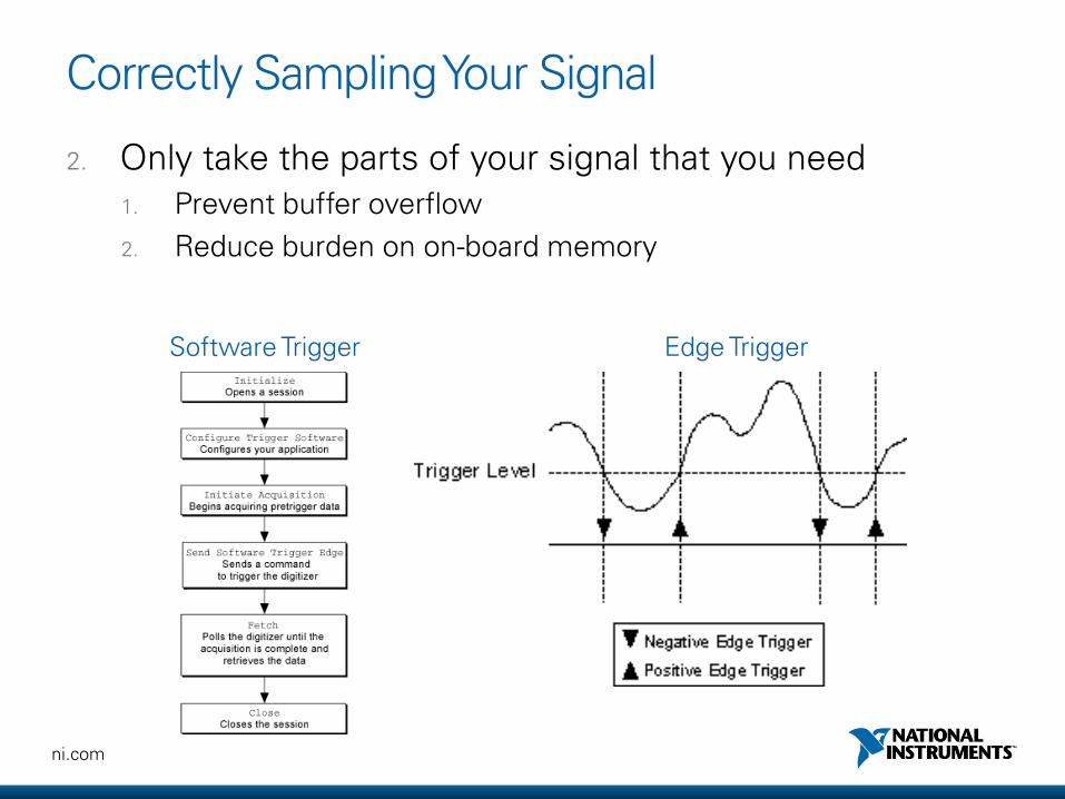
Correctly Sampling Your Signal

2. Only take the parts of your signal that you need 1. Prevent buffer overflow

2. Reduce burden on on-board memory

Software Trigger Edge Trigger

ni.com

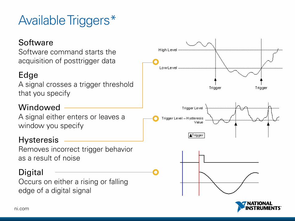
Available Triggers*

Software Software command starts the acquisition of posttrigger data

Edge A signal crosses a trigger threshold that you specify

Windowed A signal either enters or leaves a window you specify

Hysteresis Removes incorrect trigger behavior as a result of noise

Digital Occurs on either a rising or falling edge of a digital signal

ni.com

ADC Conditioning Bus

What is Digital Signal Processing (DSP)?

1. Ensure signals are correctly digitized

2. Build the right signal processing algorithm

• Choose the right FFT • Select the best window

3. Put your analysis in the right place

• Offline • Software • Inline

ni.com

Frequency Domain Analysis

Fourier’s Theorem Any waveform in the time domain can be represented by the weighted sum of sines and cosines

ni.com

Frequency Spacing and Symmetry of the FFT

1D FFT is defined as:

Frequency spacing:

where x=input sequence, N=number of elements of x, Y=transform result

where Fs=sampling rate

ni.com

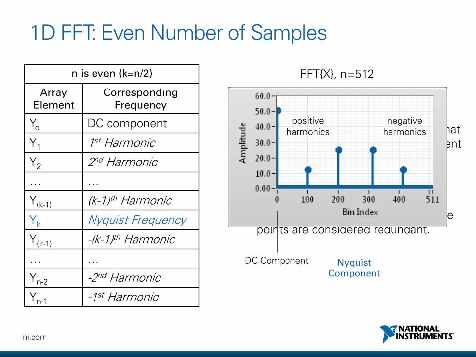
Most real-world signals have no imaginary components, and these purely real signals produce an FFT that is symmetric about the DC component at 0 Hz. This means that values at negative frequencies are exactly the same as their positive counterparts, and those points are considered redundant.

1D FFT: Even Number of Samples

n is even (k=n/2)

Array Element

Corresponding Frequency

Yo DC component

Y1 1st Harmonic

Y2 2nd Harmonic

… …

Y(k-1) (k-1)th Harmonic

Yk Nyquist Frequency

Y-(k-1) -(k-1)th Harmonic

… …

Yn-2 -2nd Harmonic

Yn-1 -1st Harmonic

FFT{X}, n=512

DC Component Nyquist Component

positive harmonics

negative harmonics

ni.com

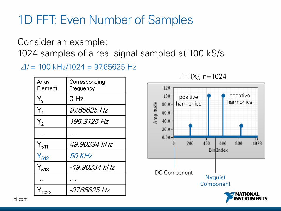
1D FFT: Even Number of Samples

Consider an example: 1024 samples of a real signal sampled at 100 kS/s

Δf = 100 kHz/1024 = 97.65625 Hz

Array Element

Corresponding Frequency

Yo

Y1

Y2

…

Y511

Y512

Y513

…

Y1023

Array Element

Corresponding Frequency

Yo 0 Hz

Y1 97.65625 Hz

Y2 195.3125 Hz

… …

Y511 49.90234 kHz

Y512 50 KHz

Y513 -49.90234 kHz

… …

Y1023 -97.65625 Hz

Array Element

Corresponding Frequency

Yo 0 Hz

Y1

Y2

…

Y511

Y512

Y513

…

Y1023

Array Element

Corresponding Frequency

Yo 0 Hz

Y1 97.65625 Hz

Y2 195.3125 Hz

… …

Y511

Y512

Y513

…

Y1023

Array Element

Corresponding Frequency

Yo 0 Hz

Y1 97.65625 Hz

Y2 195.3125 Hz

… …

Y511 49.90234 kHz

Y512 50 KHz

Y513 -49.90234 kHz

… …

Y1023

FFT{X}, n=1024

DC Component Nyquist

Component

positive harmonics

negative harmonics

ni.com

FFT{X}

DC Component kth Harmonic

positive harmonics

negative harmonics

1D FFT: Odd Number of Samples

n is odd (k=(n-1)/2)

Array Element

Corresponding Frequency

Yo DC component

Y1 1st Harmonic

Y2 2nd Harmonic

… …

Y(k-1) (k-1)th Harmonic

Yk kth Harmonic

Y-(k-1) -(k-1)th Harmonic

… …

Yn-2 -2nd Harmonic

Yn-1 -1st Harmonic

ni.com

The Power Spectrum

The power at a particular frequency component is the square of the magnitude at that component

Power is always real, and all phase information is lost

For even n (k=n/2)

Array Element Interpretation

Sxx[0] Power in DC component

Sxx[1] = Sxx[N-1] Power at 1st harmonic

Sxx[2] = Sxx[N-2] Power at 2nd harmonic

… …

Sxx[k-2] = Sxx[N-(k-2)] Power at (k-2)th harmonic

Sxx[k-1] = Sxx[N-(k-1)] Power at (k-1)th harmonic

Sxx[k] Power at (k)th harmonic

ni.com

Array-based Analysis vs Point-by-Point Analysis

Point-by-point analysis A subset of inline analysis where results are calculated after every individual sample rather than on a group of samples.

ni.com

Array-based Analysis vs Point-by-Point Analysis

Characteristics

• Limited compatibility with real-time systems

• Specify a buffer

• “Delayed” processing

• Asynchronous work style

Characteristics

• Compatible with real-time systems

• No explicit buffers

• Immediate processing

• Synchronous work style

• Must initialize

Such analysis is essential when dealing with control processes featuring high-speed, deterministic, single-point data acquisition. Latency between acquisition and decision is minimized.

Array-based Pt-by-Pt

ni.com

Spectral Leakage

Practical signals are finite, but the FFT assumes this time record repeats.

If you have an integral number of cycles in your time record, the repetition is smooth at the boundaries. If not, you get discontinuities.

ni.com

Effects of Spectral Leakage on an FFT

Power Spectrum

Power Spectrum

Non-integer number of periods

Integer number of periods

ni.com

Windowing

Windowing can be used to smooth these boundaries, reducing the size of the discontinuity and thus spectral leakage.

Power Spectrum

ni.com

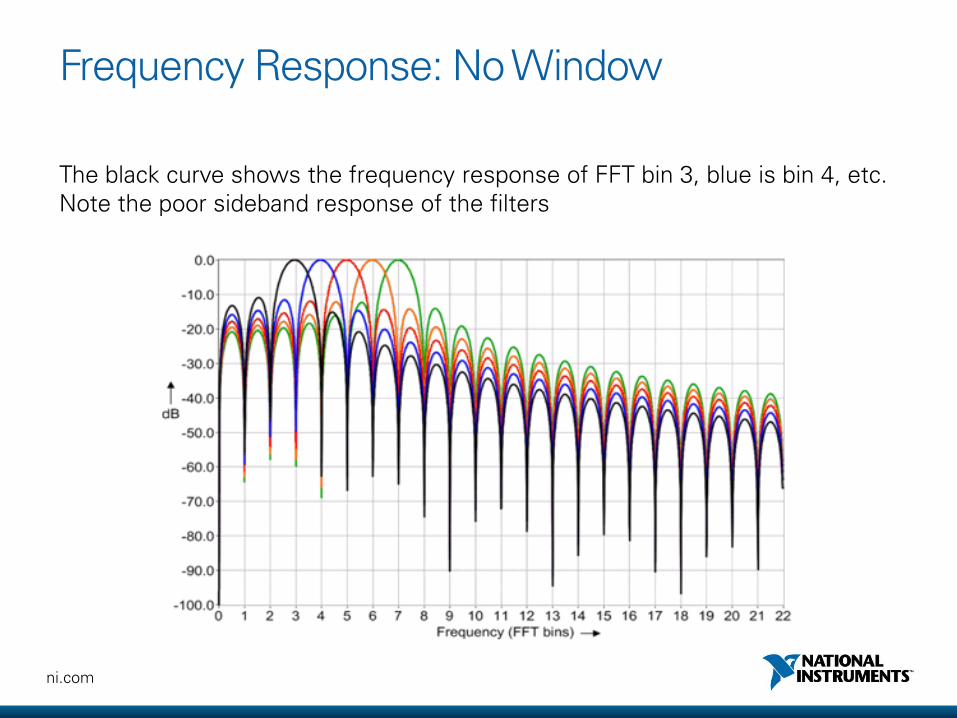
Frequency Response: No Window

The black curve shows the frequency response of FFT bin 3, blue is bin 4, etc. Note the poor sideband response of the filters

ni.com

Frequency Response: 4-term Blackman Harris

Using a 4-term Blackman Harris window before the FFT minimizes side lobes

Tradeoff: the main lobe’s -3 dB bandwidth increased from 1 bin to 2 bins

ni.com

Choosing a Filter

Signal Characteristic Window Characteristic

Strong frequency components far from your frequency of interest

Window with a high side lobe roll-off rate

Strong frequency components near your frequency of interest

Low maximum side lobe level

Area of interest is 2+ nearby frequencies Narrow main lobe to maximize spectral resolution

Amplitude accuracy of a single frequency of interest is important

Window with a wide main lobe

Flat signal, or broadband in frequency content

Uniform window or no window

Not sure? A Hanning window will do the job most of the time, and is a good starting point

ni.com

Learn More Windowing Techniques

Find a handy guide online – search “windowing fft”

Windowing: Optimizing FFTs Using Window Functions

ni.com

ADC Conditioning Bus

What is Digital Signal Processing (DSP)?

1. Ensure signals are correctly digitized

2. Build the right signal processing algorithm

• Choose the right FFT • Select the best window

3. Put your analysis in the right place

• Offline • Software • Inline

ni.com

Analysis in a Generic System Architecture

Processor FPGA

I/O

I/O

I/O

I/O

Offline

On processor during acquisition

Inline with acquisition hardware

ni.com

When Should Analysis be Offline?

Offline Analysis | Analysis performed after data acquisition

Benefits

• Not limited by timing and memory constraints of data acquisition

• Greater data interactivity. You have the ability to freely explore raw data and results of analysis

• Doesn’t bottleneck your acquisition. Offline analysis might be necessary for intensive algorithms operating on large data sets

Typical Use Cases

• Only useful when you do not need to make decisions as a result of this analysis as you acquire data

• Often used to identify the cause and effect of variables by correlating multiple data sets

• Histograms, trending, and curve-fitting are common offline analysis tasks

ni.com

Performing Analysis in Software During Acquisition

Processor FPGA

I/O

I/O

I/O

I/O

General Purpose OS Real-Time OS

• Precise timing • Higher level of determinism • Typically run one program at a time • Usually no user interface

• Can run many tasks at a time • Familiar environment • “General Purpose”

ni.com

Analyze Inline with Acquisition Hardware

Processor FPGA

I/O

I/O

I/O

I/O

Put analysis algorithms directly onto an FPGA

• True parallelism • High reliability as designs become a custom circuit • Runs algorithms at deterministic rates on the order of nanoseconds • Reconfigurable

ni.com

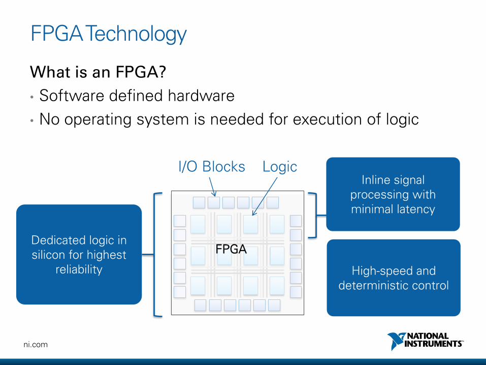
Dedicated logic in silicon for highest

reliability

FPGA Technology

What is an FPGA?

• Software defined hardware

• No operating system is needed for execution of logic

I/O Blocks Logic

High-speed and deterministic control

Inline signal processing with minimal latency

FPGA

ni.com

Mapping LabVIEW to an FPGA

W

X

Y Z

A

B

C

D

F

ni.com

FPGA Enables Data Reduction & In-line DSP

Filtering

Peak-detect

FFTs

Custom triggering

Algorithmic pattern generation

Co-processing

Modulation/demodulation

Image Sensor

LCD Display NI 6581 Adapter

Acquire Process Display

Virtex-5 LX85 FPGA Modules

ni.com

High Performance Application: Real-Time OCT Imaging

Goal: Create a medical instrument to detect cancer without the patient undergoing a stressful biopsy

A 3D optical coherence tomography (OCT) imaging system is a non-invasive solution with better resolution than traditional MRI or PET scans.

ni.com

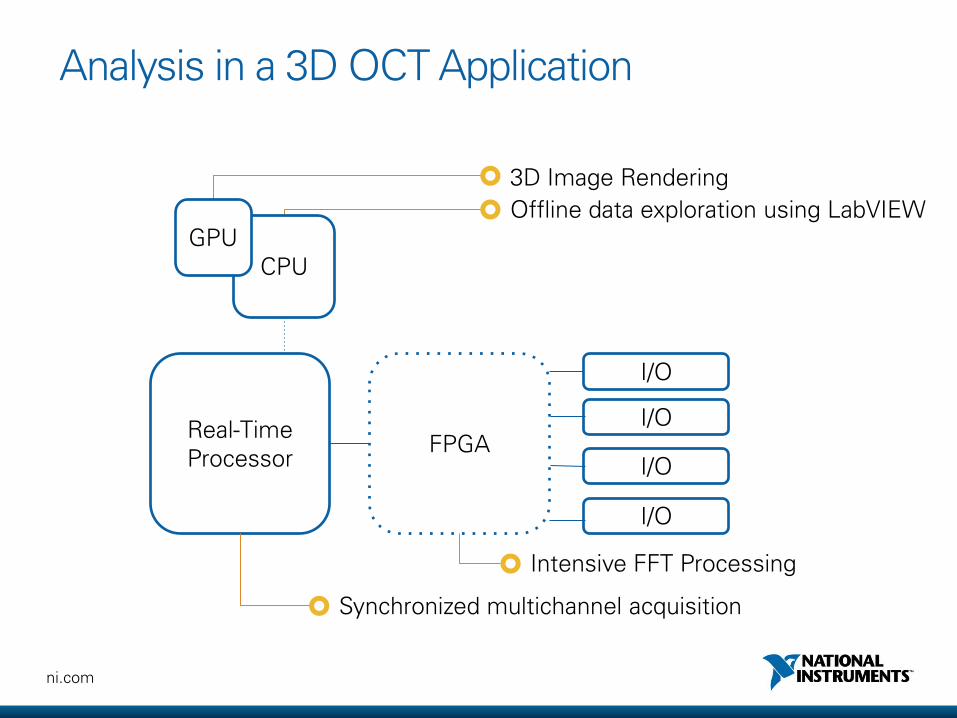
High Performance Application: Real-Time OCT Imaging

Researchers used LabVIEW to perform analysis on highly parallel computing architectures. These technologies enabled them to achieve the fast processing necessary for 3D imaging.

Used LabVIEW with NI FlexRIO to compute over 700,000 512-point FFTs every second

Real-time 3D image rendering and display was performed using a high performance NVIDIA Quadro GPU

ni.com

Analysis in a 3D OCT Application

Real-Time Processor

FPGA

I/O

I/O

I/O

I/O

Offline data exploration using LabVIEW

Synchronized multichannel acquisition

Intensive FFT Processing

3D Image Rendering

CPU GPU

ni.com

Already CLAD Certified?

You’re immediately eligible to take the Certified LabVIEW Developer exam. Start preparing now! • Join a local user group • Prepare using resources on Developer Zone

ni.com/training/certification_prep • Time yourself during practice exams

Note: CLAD certification must be current to take the CLD exam

Email certification@ni.com to register for an exam near you.

ni.com