Digital Servo Control of a Hard-Disk Drive

Open this Example

This example shows how to use Control System Toolbox™ to design a digital servo controller for a disk

drive read/write head.

For details about the system and model, see Chapter 14 of "Digital Control of Dynamic Systems," by

Franklin, Powell, and Workman.

On this page…

Disk Drive Model

Servo Controller

Discretization of Model

Controller Design

Robustness Analysis

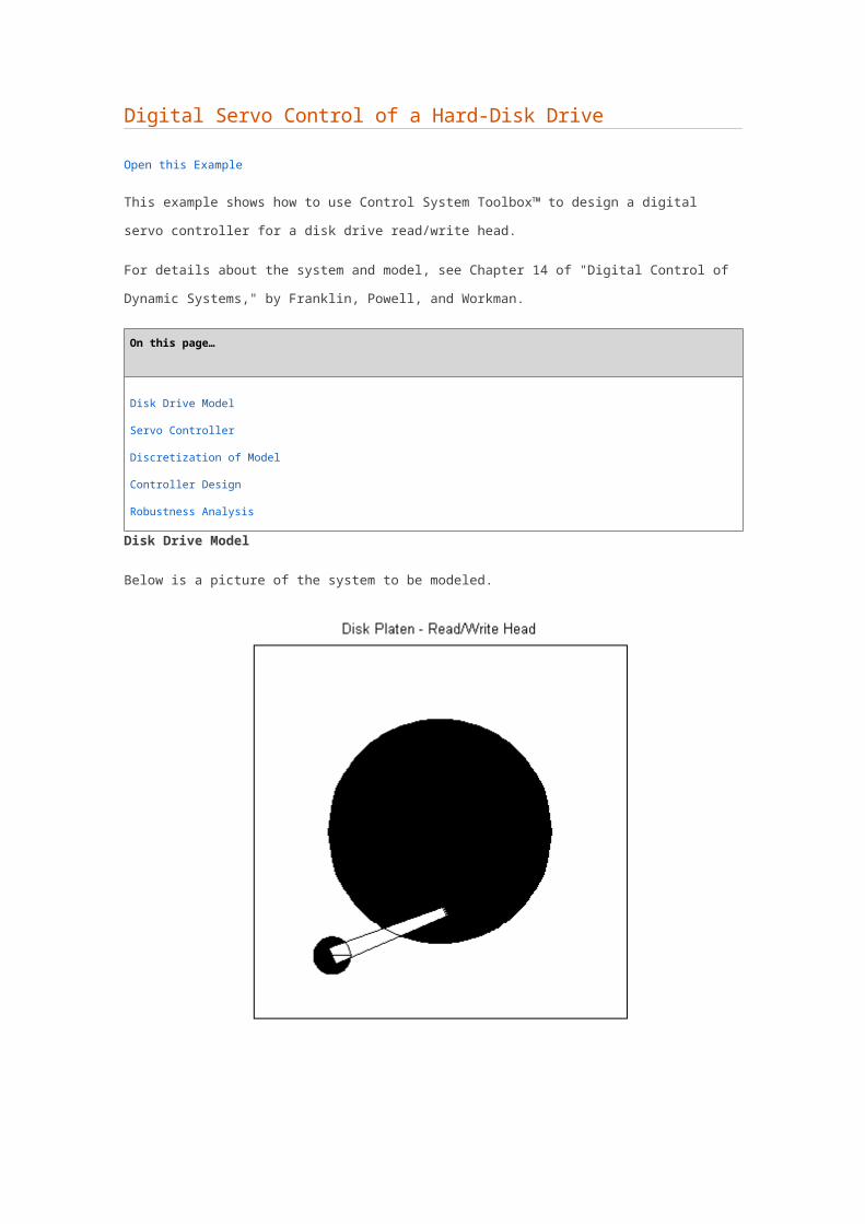
Disk Drive Model

Below is a picture of the system to be modeled.

The head-disk assembly (HDA) and actuators are modeled by a 10th-order transfer function including two

rigid-body modes and the first four resonances.

The model input is the current ic driving the voice coil motor, and the output is the position error signal

(PES, in % of track width). The model also includes a small delay.

Disk Drive Model:

The coupling coefficients, damping, and natural frequencies (in Hz) for the dominant flexible modes are

listed below.

Model Data:

Given this data, construct a nominal model of the head assembly:

load diskdemo

Gr = tf(1e6,[1 12.5 0],'outputdelay',1e-5);

Gf1 = tf(w1*[a1 b1*w1],[1 2*z1*w1 w1^2]); % first resonance

Gf2 = tf(w2*[a2 b2*w2],[1 2*z2*w2 w2^2]); % second resonance

Gf3 = tf(w3*[a3 b3*w3],[1 2*z3*w3 w3^2]); % third resonance

Gf4 = tf(w4*[a4 b4*w4],[1 2*z4*w4 w4^2]); % fourth resonance

G = Gr * (ss(Gf1) + Gf2 + Gf3 + Gf4); % convert to state

space for accuracy

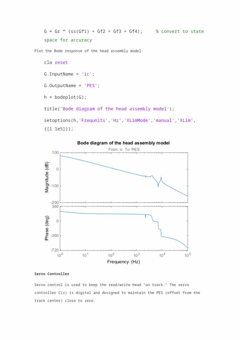
Plot the Bode response of the head assembly model:

cla reset

G.InputName = 'ic';

G.OutputName = 'PES';

h = bodeplot(G);

title('Bode diagram of the head assembly model');

setoptions(h,'Frequnits','Hz','XLimMode','manual','XLim',

{[1 1e5]});

Servo Controller

Servo control is used to keep the read/write head "on track." The servo controller C(z) is digital and

designed to maintain the PES (offset from the track center) close to zero.

The disturbance considered here is a step variation d in the input current ic. Your task is to design a digital

compensator C(z) with adequate disturbance rejection performance.

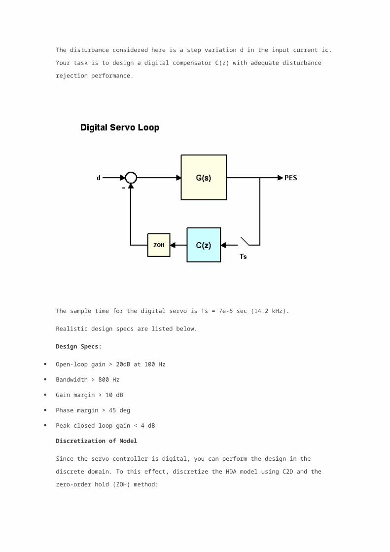
The sample time for the digital servo is Ts = 7e-5 sec (14.2 kHz).

Realistic design specs are listed below.

Design Specs:

Open-loop gain > 20dB at 100 Hz

Bandwidth > 800 Hz

Gain margin > 10 dB

Phase margin > 45 deg

Peak closed-loop gain < 4 dB

Discretization of Model

Since the servo controller is digital, you can perform the design in the discrete domain. To this effect,

discretize the HDA model using C2D and the zero-order hold (ZOH) method:

cla reset

Ts = 7e-5;

Gd = c2d(G,Ts);

h = bodeplot(G,'b',Gd,'r'); % compare with the continuous-

time model

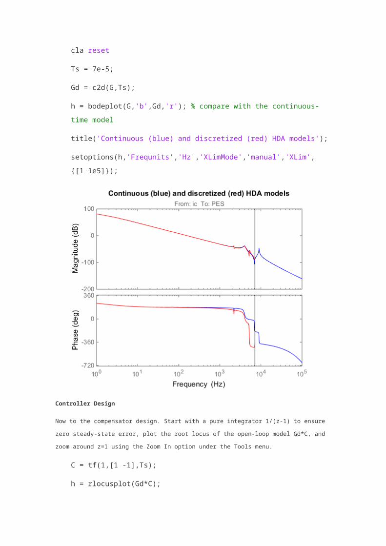
title('Continuous (blue) and discretized (red) HDA models');

setoptions(h,'Frequnits','Hz','XLimMode','manual','XLim',

{[1 1e5]});

Controller Design

Now to the compensator design. Start with a pure integrator 1/(z-1) to ensure zero steady-state error, plot

the root locus of the open-loop model Gd*C, and zoom around z=1 using the Zoom In option under the

Tools menu.

C = tf(1,[1 -1],Ts);

h = rlocusplot(Gd*C);

setoptions(h,'Grid','on','XLimMode','Manual','XLim',{[-

1.5,1.5]},...

'YLimMode','Manual','YLim',{[-1,1]});

Because of the two poles at z=1, the servo loop is unstable for all positive gains. To stabilize the feedback

loop, first add a pair of zeros near z=1.

C = C * zpk([.963,.963],-0.706,1,Ts);

h = rlocusplot(Gd*C);

setoptions(h,'Grid','on','XLimMode','Manual','XLim',{[-

1.25,1.25]},...

'YLimMode','Manual','YLim',{[-1.2,1.2]});

Next adjust the loop gain by clicking on the locus and dragging the black square inside the unit circle. The

loop gain is displayed in the data marker. A gain of approximately 50 stabilizes the loop (set C1 = 50*C).

C1 = 50 * C;

Now simulate the closed-loop response to a step disturbance in current. The disturbance is smoothly

rejected, but the PES is too large (head deviates from track center by 45% of track width).

cl_step = feedback(Gd,C1);

h = stepplot(cl_step);

title('Rejection of a step disturbance (PES = position

error)')

setoptions(h

,'Xlimmode','auto','Ylimmode','auto','Grid','off');

Next look at the open-loop Bode response and the stability margins. The gain at 100 Hz is only 15 dB (vs.

spec of 20 dB) and the gain margin is only 7dB, so increasing the loop gain is not an option.

margin(Gd*C1)

diskdemo_aux1(1);

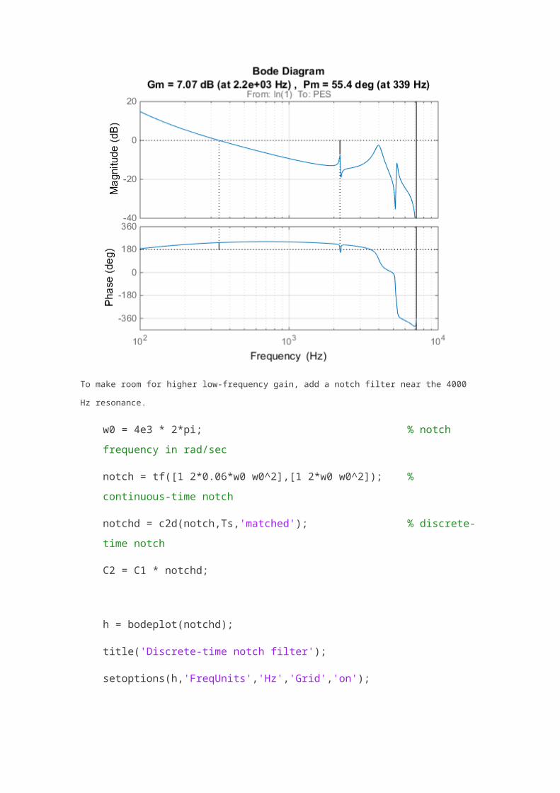
To make room for higher low-frequency gain, add a notch filter near the 4000 Hz resonance.

w0 = 4e3 * 2*pi; % notch

frequency in rad/sec

notch = tf([1 2*0.06*w0 w0^2],[1 2*w0 w0^2]); %

continuous-time notch

notchd = c2d(notch,Ts,'matched'); % discrete-

time notch

C2 = C1 * notchd;

h = bodeplot(notchd);

title('Discrete-time notch filter');

setoptions(h,'FreqUnits','Hz','Grid','on');

You can now safely double the loop gain. The resulting stability margins and gain at 100 Hz are within

specs.

C2 = 2 * C2;

margin(Gd * C2)

diskdemo_aux1(2);

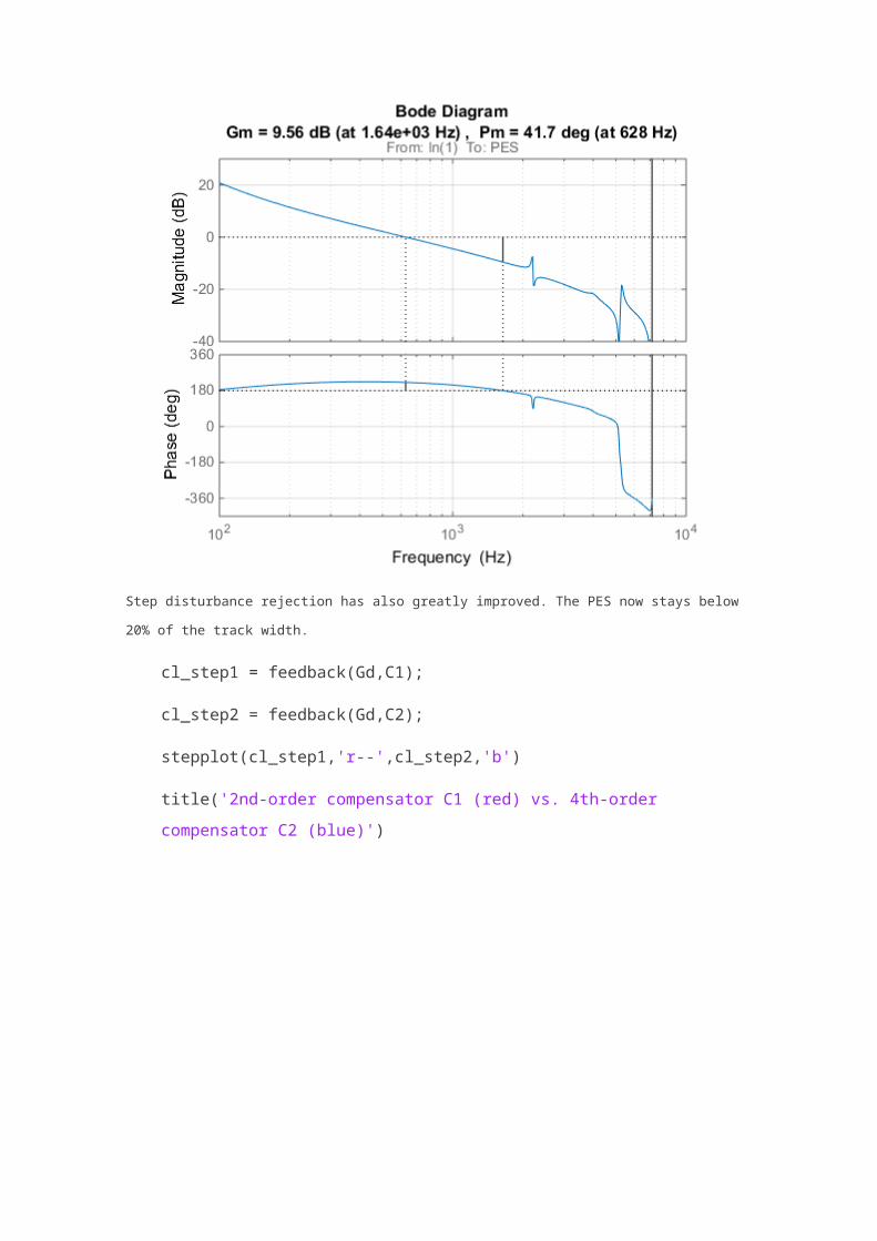
Step disturbance rejection has also greatly improved. The PES now stays below 20% of the track width.

cl_step1 = feedback(Gd,C1);

cl_step2 = feedback(Gd,C2);

stepplot(cl_step1,'r--',cl_step2,'b')

title('2nd-order compensator C1 (red) vs. 4th-order

compensator C2 (blue)')

Check if the 3dB peak gain spec on T = Gd*C/(1+Gd*C) (closed-loop sensitivity) is met:

Gd = c2d(G,Ts);

Ts = 7e-5;

T = feedback(Gd*C2,1);

h = bodeplot(T);

title('Peak response of closed-loop sensitivity T(s)')

setoptions(h

,'PhaseVisible','off','FreqUnits','Hz','Grid','on', ...

'XLimMode','Manual','XLim',{[1e2 1e4]});

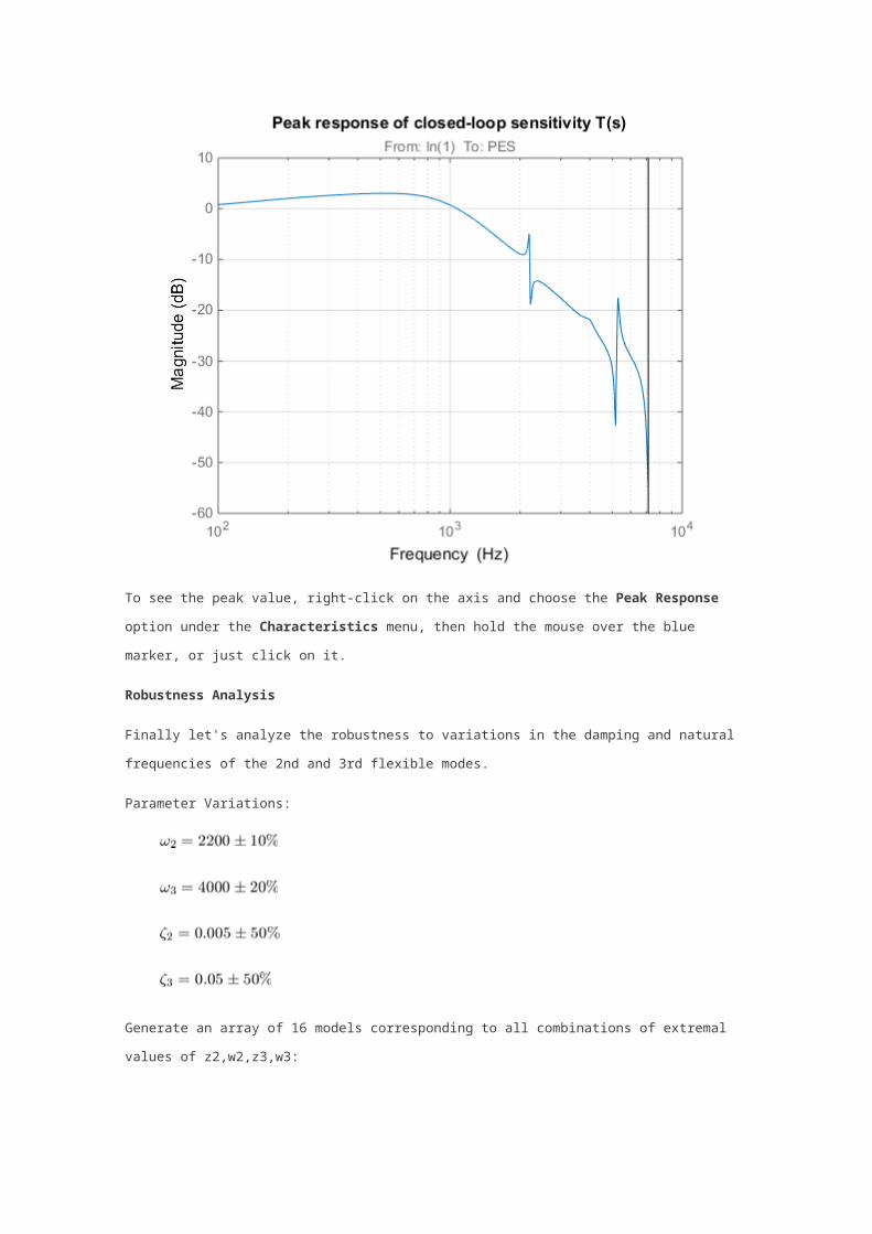
To see the peak value, right-click on the axis and choose the Peak Response option under the

Characteristics menu, then hold the mouse over the blue marker, or just click on it.

Robustness Analysis

Finally let's analyze the robustness to variations in the damping and natural frequencies of the 2nd and 3rd

flexible modes.

Parameter Variations:

Generate an array of 16 models corresponding to all combinations of extremal values of z2,w2,z3,w3:

[z2,w2,z3,w3] = ndgrid([.5*z2,1.5*z2],[.9*w2,1.1*w2],

[.5*z3,1.5*z3],[.8*w3,1.2*w3]);

for j = 1:16,

Gf21(:,:,j) = tf(w2(j)*[a2 b2*w2(j)] , [1 2*z2(j)*w2(j)

w2(j)^2]);

Gf31(:,:,j) = tf(w3(j)*[a3 b3*w3(j)] , [1 2*z3(j)*w3(j)

w3(j)^2]);

end

G1 = Gr * (ss(Gf1) + Gf21 + Gf31 + Gf4);

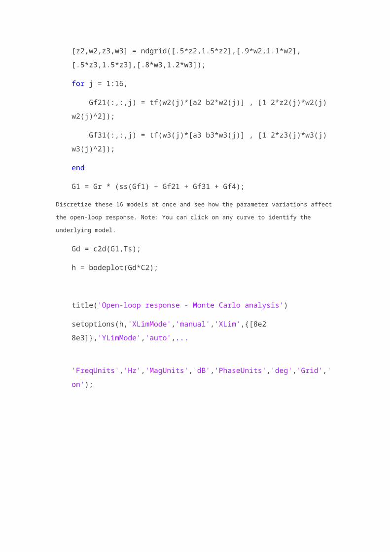
Discretize these 16 models at once and see how the parameter variations affect the open-loop response.

Note: You can click on any curve to identify the underlying model.

Gd = c2d(G1,Ts);

h = bodeplot(Gd*C2);

title('Open-loop response - Monte Carlo analysis')

setoptions(h,'XLimMode','manual','XLim',{[8e2

8e3]},'YLimMode','auto',...

'FreqUnits

','Hz','MagUnits','dB','PhaseUnits','deg','Grid','on');

Plot the step disturbance rejection performance for these 16 models:

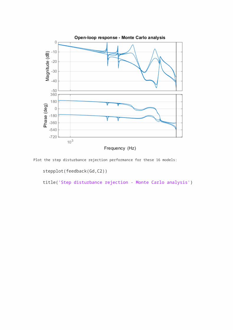
stepplot(feedback(Gd,C2))

title('Step disturbance rejection - Monte Carlo analysis')

Tuning of a Digital Motion Control System

This example shows how to use Robust Control Toolbox™ to tune a digital motion control system.

On this page…

Motion Control System

Compensator Tuning

Design Validation

Tuning an Additional Notch Filter

Discretizing the Notch Filter

Discrete-Time Tuning

Motion Control System

The motion system under consideration is shown below.

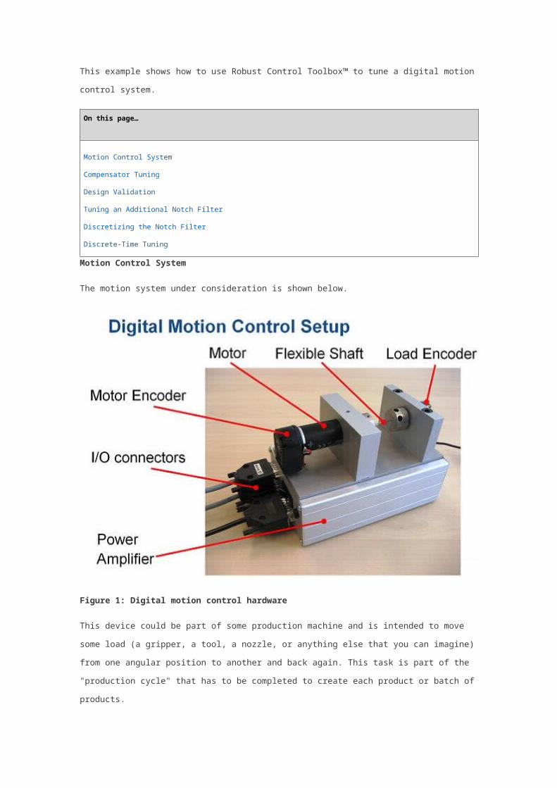
Figure 1: Digital motion control hardware

This device could be part of some production machine and is intended to move some load (a gripper, a

tool, a nozzle, or anything else that you can imagine) from one angular position to another and back again.

This task is part of the "production cycle" that has to be completed to create each product or batch of

products.

The digital controller must be tuned to maximize the production speed of the machine without

compromising accuracy and product quality. To do this, we first model the control system in Simulink using

a 4th-order model of the inertia and flexible shaft:

open_system('rct_dmc')

The "Tunable Digital Controller" consists of a gain in series with a lead/lag controller.

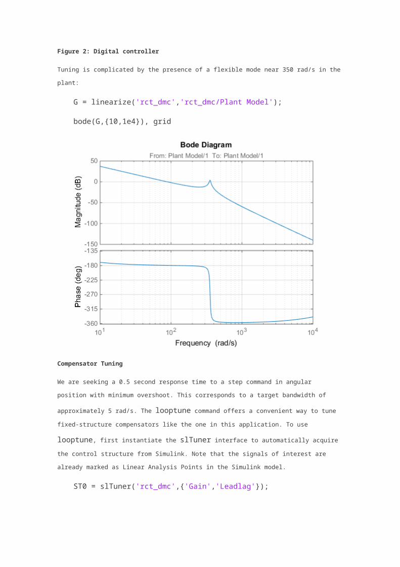
Figure 2: Digital controller

Tuning is complicated by the presence of a flexible mode near 350 rad/s in the plant:

G = linearize('rct_dmc','rct_dmc/Plant Model');

bode(G,{10,1e4}), grid

Compensator Tuning

We are seeking a 0.5 second response time to a step command in angular position with minimum

overshoot. This corresponds to a target bandwidth of approximately 5 rad/s. The looptune command

offers a convenient way to tune fixed-structure compensators like the one in this application. To use

looptune, first instantiate the slTuner interface to automatically acquire the control structure from

Simulink. Note that the signals of interest are already marked as Linear Analysis Points in the Simulink

model.

ST0 = slTuner('rct_dmc',{'Gain','Leadlag'});

Next use looptune to tune the compensator parameters for the target gain crossover frequency of 5

rad/s:

Measurement = 'Measured Position'; % controller input

Control = 'Leadlag'; % controller output

ST1 = looptune(ST0,Control,Measurement,5);

Final: Peak gain = 0.975, Iterations = 21

Achieved target gain value TargetGain=1.

A final value below or near 1 indicates success. Inspect the tuned values of the gain and lead/lag filter:

showBlockValue(ST1)

AnalysisPoints_ =

d =

u1 u2 u3 u4 u5

y1 1 0 0 0 0

y2 0 1 0 0 0

y3 0 0 1 0 0

y4 0 0 0 1 0

y5 0 0 0 0 1

Name: AnalysisPoints_

Static gain.

-----------------------------------

Gain =

d =

u1

y1 2.753e-06

Name: Gain

Static gain.

-----------------------------------

Leadlag =

30.54 s + 59.01

---------------

s + 18.94

Name: Leadlag

Continuous-time transfer function.

Design Validation

To validate the design, use the slTuner interface to quickly access the closed-loop transfer functions of

interest and compare the responses before and after tuning.

T0 = getIOTransfer(ST0,'Reference','Measured Position');

T1 = getIOTransfer(ST1,'Reference','Measured Position');

step(T0,T1), grid

legend('Original','Tuned')

The tuned response has significantly less overshoot and satisfies the response time requirement. However

these simulations are obtained using a continuous-time lead/lag compensator (looptune operates in

continuous time) so we need to further validate the design in Simulink using a digital implementation of the

lead/lag compensator. Use writeBlockValue to apply the tuned values to the Simulink model and

automatically discretize the lead/lag compensator to the rate specified in Simulink.

writeBlockValue(ST1)

You can now simulate the response of the continuous-time plant with the digital controller:

sim('rct_dmc'); % angular position logged in "yout"

variable

t = yout.time;

y = yout.signals.values;

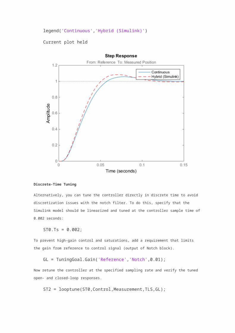
step(T1), hold, plot(t,y,'r--')

legend('Continuous','Hybrid (Simulink)')

Current plot held

The simulations closely match and the coefficients of the digital lead/lag can be read from the "Leadlag"

block in Simulink.

Tuning an Additional Notch Filter

Next try to increase the control bandwidth from 5 to 50 rad/s. Because of the plant resonance near 350

rad/s, the lead/lag compensator is no longer sufficient to get adequate stability margins and small

overshoot. One remedy is to add a notch filter as shown in Figure 3.

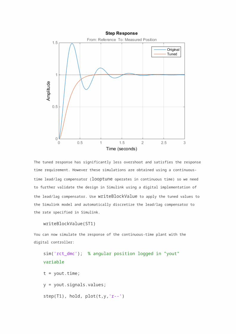
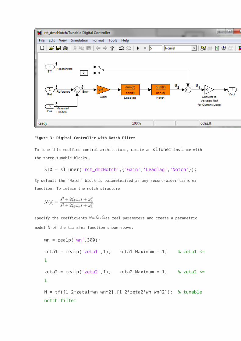
Figure 3: Digital Controller with Notch Filter

To tune this modified control architecture, create an slTuner instance with the three tunable blocks.

ST0 = slTuner('rct_dmcNotch',{'Gain','Leadlag','Notch'});

By default the "Notch" block is parameterized as any second-order transfer function. To retain the notch

structure

specify the coefficients as real parameters and create a parametric model N of the transfer

function shown above:

wn = realp('wn',300);

zeta1 = realp('zeta1',1); zeta1.Maximum = 1; % zeta1 <=

1

zeta2 = realp('zeta2',1); zeta2.Maximum = 1; % zeta2 <=

1

N = tf([1 2*zeta1*wn wn^2],[1 2*zeta2*wn wn^2]); % tunable

notch filter

Then associate this parametric notch model with the "Notch" block in the Simulink model. Because the

control system is tuned in the continuous time, you can use a continuous-time parameterization of the

notch filter even though the "Notch" block itself is discrete.

setBlockParam(ST0,'Notch',N);

Next use looptune to jointly tune the "Gain", "Leadlag", and "Notch" blocks with a 50 rad/s target

crossover frequency. To eliminate residual oscillations from the plant resonance, specify a target loop

shape with a -40 dB/decade roll-off past 50 rad/s.

% Specify target loop shape with a few frequency points

Freqs = [5 50 500];

Gains = [10 1 0.01];

TLS = TuningGoal.LoopShape('Notch',frd(Gains,Freqs));

Measurement = 'Measured Position'; % controller input

Control = 'Notch'; % controller output

ST2 = looptune(ST0,Control,Measurement,TLS);

Final: Peak gain = 1.05, Iterations = 69

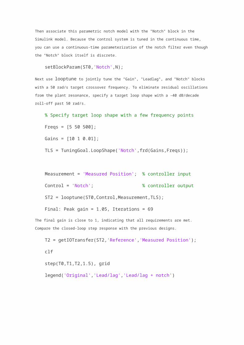
The final gain is close to 1, indicating that all requirements are met. Compare the closed-loop step

response with the previous designs.

T2 = getIOTransfer(ST2,'Reference','Measured Position');

clf

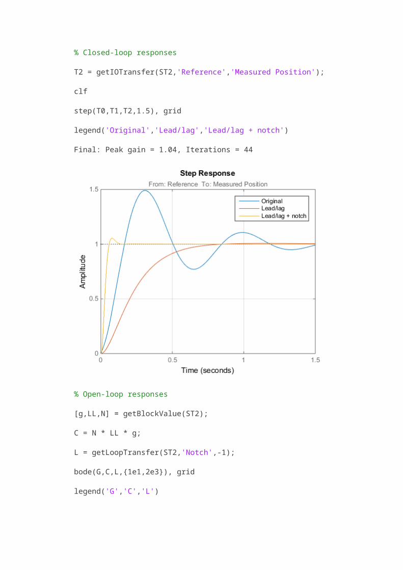
step(T0,T1,T2,1.5), grid

legend('Original','Lead/lag','Lead/lag + notch')

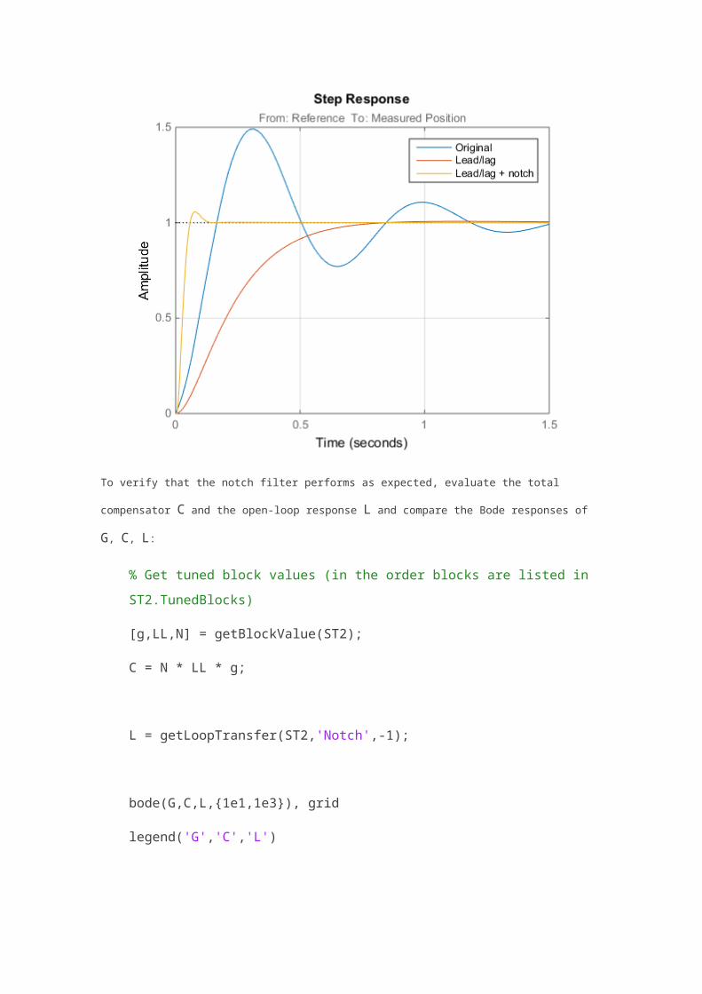
To verify that the notch filter performs as expected, evaluate the total compensator C and the open-loop

response L and compare the Bode responses of G, C, L:

% Get tuned block values (in the order blocks are listed in

ST2.TunedBlocks)

[g,LL,N] = getBlockValue(ST2);

C = N * LL * g;

L = getLoopTransfer(ST2,'Notch',-1);

bode(G,C,L,{1e1,1e3}), grid

legend('G','C','L')

This Bode plot confirms that the plant resonance has been correctly "notched out."

Discretizing the Notch Filter

Again use writeBlockValue to discretize the tuned lead/lag and notch filters and write their values

back to Simulink. Compare the MATLAB and Simulink responses:

writeBlockValue(ST2)

sim('rct_dmcNotch');

t = yout.time;

y = yout.signals.values;

step(T2), hold, plot(t,y,'r--')

legend('Continuous','Hybrid (Simulink)')

Current plot held

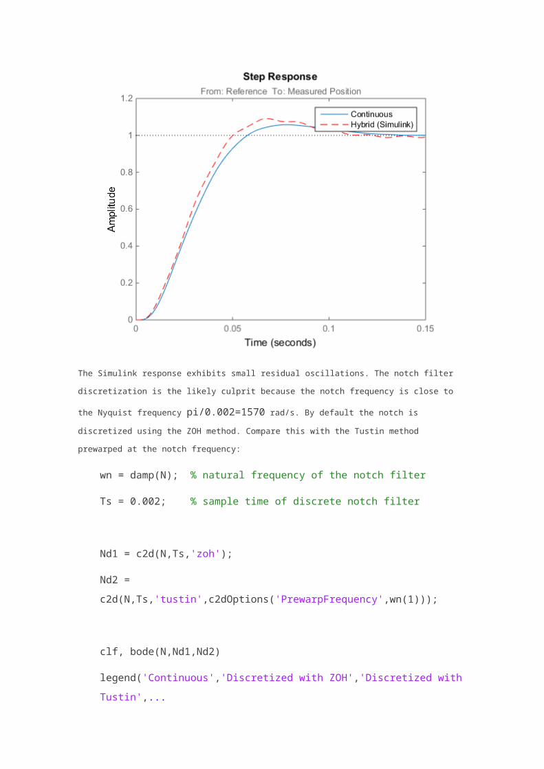
The Simulink response exhibits small residual oscillations. The notch filter discretization is the likely culprit

because the notch frequency is close to the Nyquist frequency pi/0.002=1570 rad/s. By default the

notch is discretized using the ZOH method. Compare this with the Tustin method prewarped at the notch

frequency:

wn = damp(N); % natural frequency of the notch filter

Ts = 0.002; % sample time of discrete notch filter

Nd1 = c2d(N,Ts,'zoh');

Nd2 =

c2d(N,Ts,'tustin',c2dOptions('PrewarpFrequency',wn(1)));

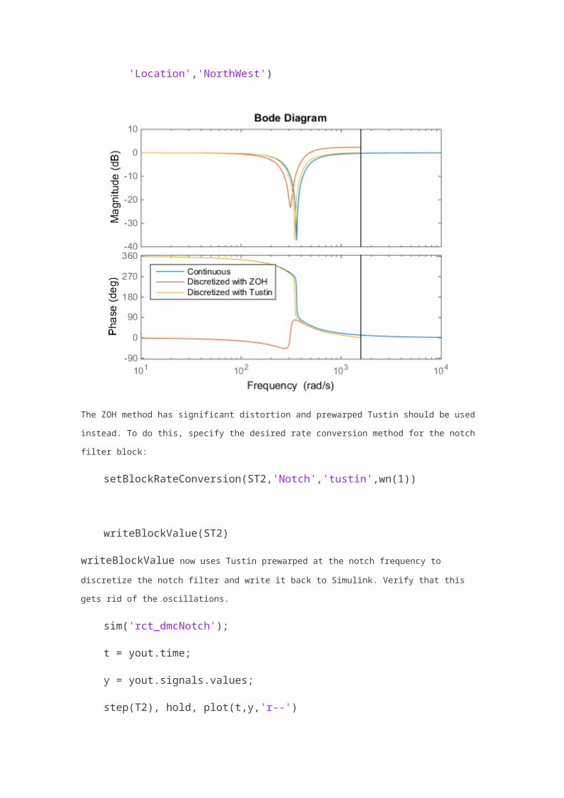
clf, bode(N,Nd1,Nd2)

legend('Continuous','Discretized with ZOH','Discretized with

Tustin',...

'Location','NorthWest')

The ZOH method has significant distortion and prewarped Tustin should be used instead. To do this,

specify the desired rate conversion method for the notch filter block:

setBlockRateConversion(ST2,'Notch','tustin',wn(1))

writeBlockValue(ST2)

writeBlockValue now uses Tustin prewarped at the notch frequency to discretize the notch filter

and write it back to Simulink. Verify that this gets rid of the oscillations.

sim('rct_dmcNotch');

t = yout.time;

y = yout.signals.values;

step(T2), hold, plot(t,y,'r--')

legend('Continuous','Hybrid (Simulink)')

Current plot held

Discrete-Time Tuning

Alternatively, you can tune the controller directly in discrete time to avoid discretization issues with the

notch filter. To do this, specify that the Simulink model should be linearized and tuned at the controller

sample time of 0.002 seconds:

ST0.Ts = 0.002;

To prevent high-gain control and saturations, add a requirement that limits the gain from reference to

control signal (output of Notch block).

GL = TuningGoal.Gain('Reference','Notch',0.01);

Now retune the controller at the specified sampling rate and verify the tuned open- and closed-loop

responses.

ST2 = looptune(ST0,Control,Measurement,TLS,GL);

% Closed-loop responses

T2 = getIOTransfer(ST2,'Reference','Measured Position');

clf

step(T0,T1,T2,1.5), grid

legend('Original','Lead/lag','Lead/lag + notch')

Final: Peak gain = 1.04, Iterations = 44

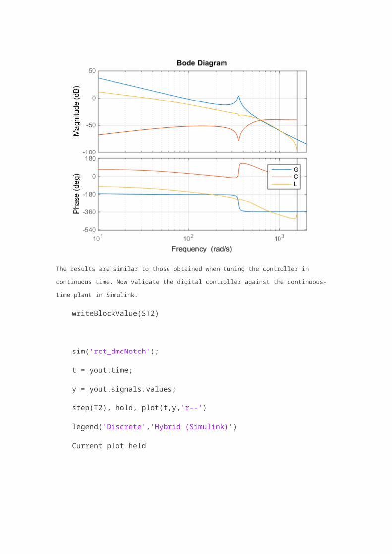
% Open-loop responses

[g,LL,N] = getBlockValue(ST2);

C = N * LL * g;

L = getLoopTransfer(ST2,'Notch',-1);

bode(G,C,L,{1e1,2e3}), grid

legend('G','C','L')

The results are similar to those obtained when tuning the controller in continuous time. Now validate the

digital controller against the continuous-time plant in Simulink.

writeBlockValue(ST2)

sim('rct_dmcNotch');

t = yout.time;

y = yout.signals.values;

step(T2), hold, plot(t,y,'r--')

legend('Discrete','Hybrid (Simulink)')

Current plot held

This time, the hybrid response closely matches its discrete-time approximation and no further adjustment

of the notch filter is required.

Multi-Loop PID Control of a Robot Arm

This example shows how to use looptune to tune a multi-loop controller for a 4-DOF robotic arm

manipulator.

On this page…

Robotic Arm Model and Controller

Linearizing the Plant

Tuning the PID Controllers with LOOPTUNE

Exploiting the Second Degree of Freedom

Validating the Tuned Controller

Refining The Design

Robotic Arm Model and Controller

This example uses the four degree-of-freedom robotic arm shown below. This arm consists of four joints

labeled from base to tip: "Turntable", "Bicep", "Forearm", and "Wrist". Each joint is actuated by a DC motor

except for the Bicep joint which uses two DC motors in tandem.

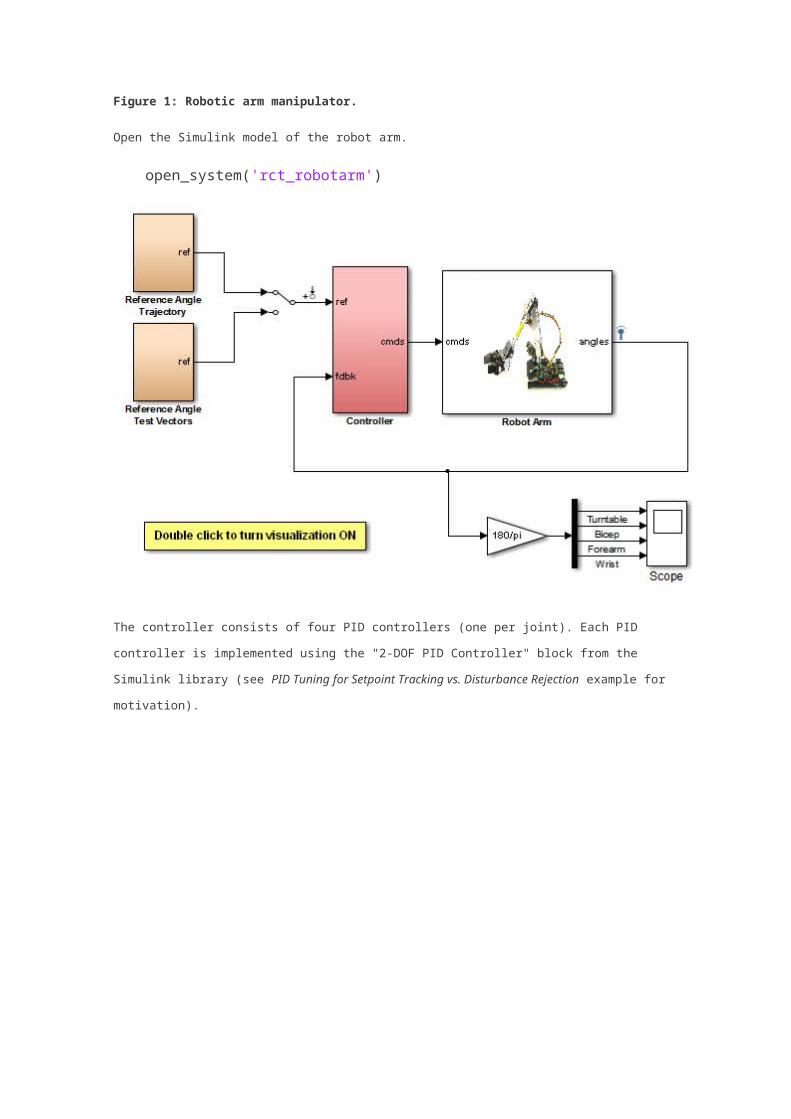
Figure 1: Robotic arm manipulator.

Open the Simulink model of the robot arm.

open_system('rct_robotarm')

The controller consists of four PID controllers (one per joint). Each PID controller is implemented using the

"2-DOF PID Controller" block from the Simulink library (see PID Tuning for Setpoint Tracking vs.

Disturbance Rejection example for motivation).

Figure 2: Controller structure.

Typically, such multi-loop controllers are tuned sequentially by tuning one PID loop at a time and cycling

through the loops until the overall behavior is satisfactory. This process can be time consuming and is not

guaranteed to converge to the best overall tuning. Alternatively, you can use systune or looptune

to jointly tune all four PID loops subject to system-level requirements such as response time and minimum

cross-coupling.

In this example, the arm must move to a particular configuration in about 1 second with smooth angular

motion at each joint. The arm starts in a fully extended vertical position with all joint angles at zero. The

end configuration is specified by the angular positions: Turntable = 60 deg, Bicep = -10 deg, Forearm = 60

deg, Wrist = 90 deg. The angular trajectories for the original PID settings are shown below. Clearly the

response is too sluggish and the forearm is wobbling.

Figure 3: Untuned angular response.

Linearizing the Plant

The robot arm dynamics are nonlinear. To understand whether the arm can be controlled with one set of

PID gains, linearize the plant at various points (snapshot times) along the trajectory of interest. Here

"plant" refers to the dynamics between the control signals (outputs of PID blocks) and the measurement

signals (output of "Robot Arm" block).

SnapshotTimes = 0:1:5;

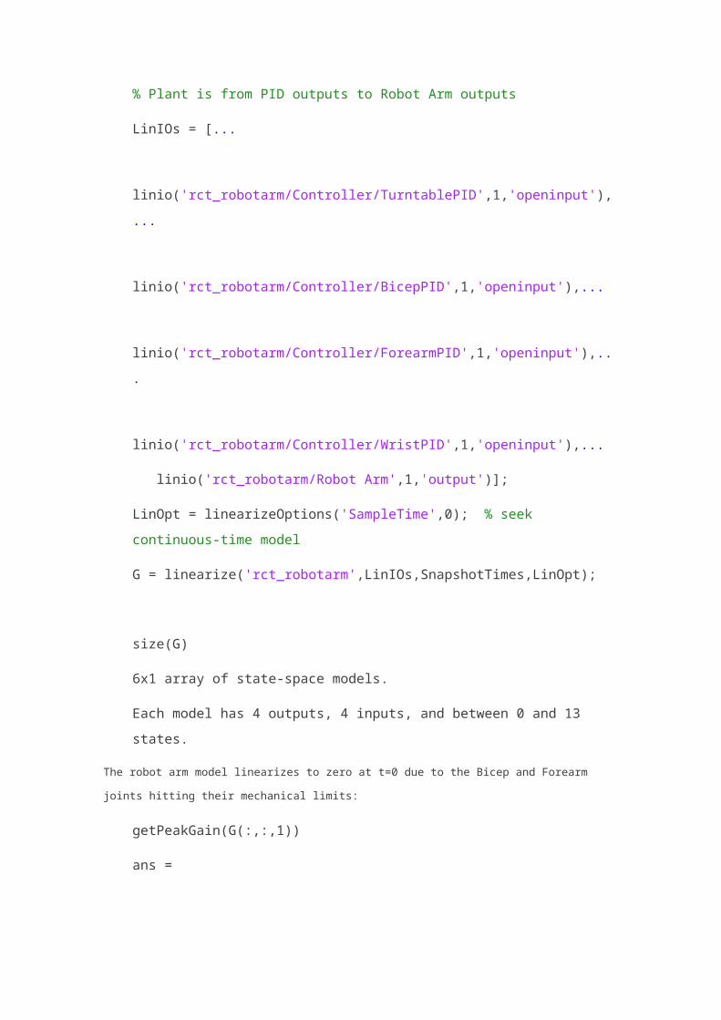
% Plant is from PID outputs to Robot Arm outputs

LinIOs = [...

linio

('rct_robotarm/Controller/TurntablePID',1,'openinput'),...

linio('rct_robotarm/Controller/BicepPID',1,'openinput'),...

linio

('rct_robotarm/Controller/ForearmPID',1,'openinput'),...

linio('rct_robotarm/Controller/WristPID',1,'openinput'),...

linio('rct_robotarm/Robot Arm',1,'output')];

LinOpt = linearizeOptions('SampleTime',0); % seek

continuous-time model

G = linearize('rct_robotarm',LinIOs,SnapshotTimes,LinOpt);

size(G)

6x1 array of state-space models.

Each model has 4 outputs, 4 inputs, and between 0 and 13

states.

The robot arm model linearizes to zero at t=0 due to the Bicep and Forearm joints hitting their mechanical

limits:

getPeakGain(G(:,:,1))

ans =

0

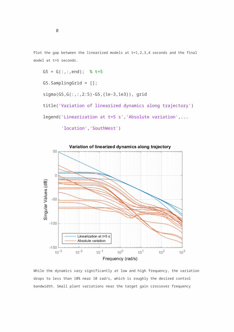
Plot the gap between the linearized models at t=1,2,3,4 seconds and the final model at t=5 seconds.

G5 = G(:,:,end); % t=5

G5.SamplingGrid = [];

sigma(G5,G(:,:,2:5)-G5,{1e-3,1e3}), grid

title('Variation of linearized dynamics along trajectory')

legend('Linearization at t=5 s','Absolute variation',...

'location','SouthWest')

While the dynamics vary significantly at low and high frequency, the variation drops to less than 10% near

10 rad/s, which is roughly the desired control bandwidth. Small plant variations near the target gain

crossover frequency suggest that we can control the arm with a single set of PID gains and need not resort

to gain scheduling.

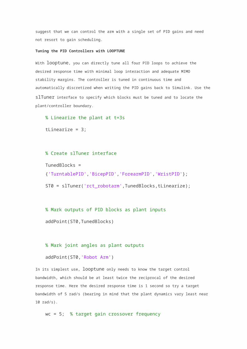
Tuning the PID Controllers with LOOPTUNE

With looptune, you can directly tune all four PID loops to achieve the desired response time with

minimal loop interaction and adequate MIMO stability margins. The controller is tuned in continuous time

and automatically discretized when writing the PID gains back to Simulink. Use the slTuner interface to

specify which blocks must be tuned and to locate the plant/controller boundary.

% Linearize the plant at t=3s

tLinearize = 3;

% Create slTuner interface

TunedBlocks =

{'TurntablePID','BicepPID','ForearmPID','WristPID'};

ST0 = slTuner('rct_robotarm',TunedBlocks,tLinearize);

% Mark outputs of PID blocks as plant inputs

addPoint(ST0,TunedBlocks)

% Mark joint angles as plant outputs

addPoint(ST0,'Robot Arm')

In its simplest use, looptune only needs to know the target control bandwidth, which should be at least

twice the reciprocal of the desired response time. Here the desired response time is 1 second so try a

target bandwidth of 5 rad/s (bearing in mind that the plant dynamics vary least near 10 rad/s).

wc = 5; % target gain crossover frequency

Controls = TunedBlocks; % actuator commands

Measurements = 'Robot Arm'; % joint angle measurements

ST1 = looptune(ST0,Controls,Measurements,wc);

Final: Peak gain = 1, Iterations = 57

Achieved target gain value TargetGain=1.

A final value near or below 1 indicates that looptune achieved the requested bandwidth. Compare the

responses to a step command in angular position for the initial and tuned controllers.

RefSignals = {'tREF','bREF','fREF','wREF'};

T0 = getIOTransfer(ST0,RefSignals,'Robot Arm');

T1 = getIOTransfer(ST1,RefSignals,'Robot Arm');

opt = timeoptions; opt.IOGrouping = 'all'; opt.Grid = 'on';

stepplot(T0,'b--',T1,'r',4,opt)

legend('Initial','Tuned','location','SouthEast')

The four curves settling near y=1 represent the step responses of each joint, and the curves settling near

y=0 represent the cross-coupling terms. The tuned controller is a clear improvement but should ideally

settle faster with less overshoot.

Exploiting the Second Degree of Freedom

The 2-DOF PID controllers have a feedforward and a feedback component.

Figure 4: Two degree-of-freedom PID controllers.

By default, looptune only tunes the feedback loop and does not "see" the feedforward component.

This can be confirmed by verifying that the and parameters of the PID controllers remain set to their

initial value (use showTunable for this purpose). To take advantage of the feedforward

action and reduce overshoot, replace the bandwidth target by an explicit tracking requirement from

reference angles to joint angles.

TR = TuningGoal.Tracking(RefSignals,'Robot Arm',0.5);

ST2 = looptune(ST0,Controls,Measurements,TR);

Final: Peak gain = 1.06, Iterations = 65

T2 = getIOTransfer(ST2,RefSignals,'Robot Arm');

stepplot(T1,'r--',T2,'g',4,opt)

legend('1-DOF tuning','2-DOF tuning','location','SouthEast')

The 2-DOF tuning reduces overshoot and takes advantage of the and parameters as confirmed by

inspecting the tuned PID gains:

showTunable(ST2)

Block 1: rct_robotarm/Controller/TurntablePID =

1 s

u = Kp (b*r-y) + Ki --- (r-y) + Kd -------- (c*r-y)

s Tf*s+1

with Kp = 13.5017, Ki = 12.9021, Kd = 0.54464, Tf =

0.030154, b = 0.85779, c = 2.0038.

Continuous-time 2-DOF PID controller.

-----------------------------------

Block 2: rct_robotarm/Controller/BicepPID =

1 s

u = Kp (b*r-y) + Ki --- (r-y) + Kd -------- (c*r-y)

s Tf*s+1

with Kp = 13.2708, Ki = 6.8389, Kd = 1.5882, Tf = 0.61258,

b = 0.72416, c = 1.5889.

Continuous-time 2-DOF PID controller.

-----------------------------------

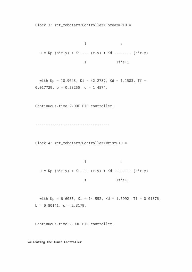
Block 3: rct_robotarm/Controller/ForearmPID =

1 s

u = Kp (b*r-y) + Ki --- (r-y) + Kd -------- (c*r-y)

s Tf*s+1

with Kp = 18.9643, Ki = 42.2787, Kd = 1.1583, Tf =

0.017729, b = 0.58255, c = 1.4574.

Continuous-time 2-DOF PID controller.

-----------------------------------

Block 4: rct_robotarm/Controller/WristPID =

1 s

u = Kp (b*r-y) + Ki --- (r-y) + Kd -------- (c*r-y)

s Tf*s+1

with Kp = 6.6085, Ki = 14.552, Kd = 1.6992, Tf = 0.01376,

b = 0.80141, c = 2.3179.

Continuous-time 2-DOF PID controller.

Validating the Tuned Controller

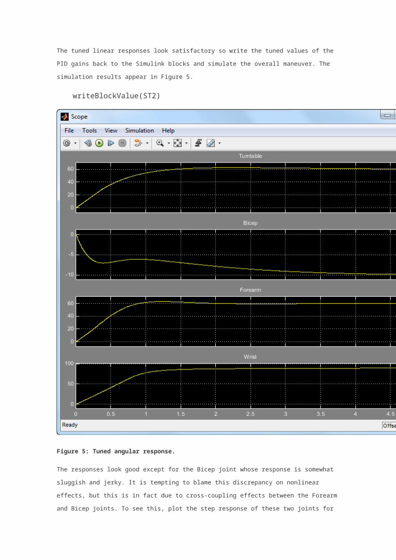
The tuned linear responses look satisfactory so write the tuned values of the PID gains back to the

Simulink blocks and simulate the overall maneuver. The simulation results appear in Figure 5.

writeBlockValue(ST2)

Figure 5: Tuned angular response.

The responses look good except for the Bicep joint whose response is somewhat sluggish and jerky. It is

tempting to blame this discrepancy on nonlinear effects, but this is in fact due to cross-coupling effects

between the Forearm and Bicep joints. To see this, plot the step response of these two joints for the

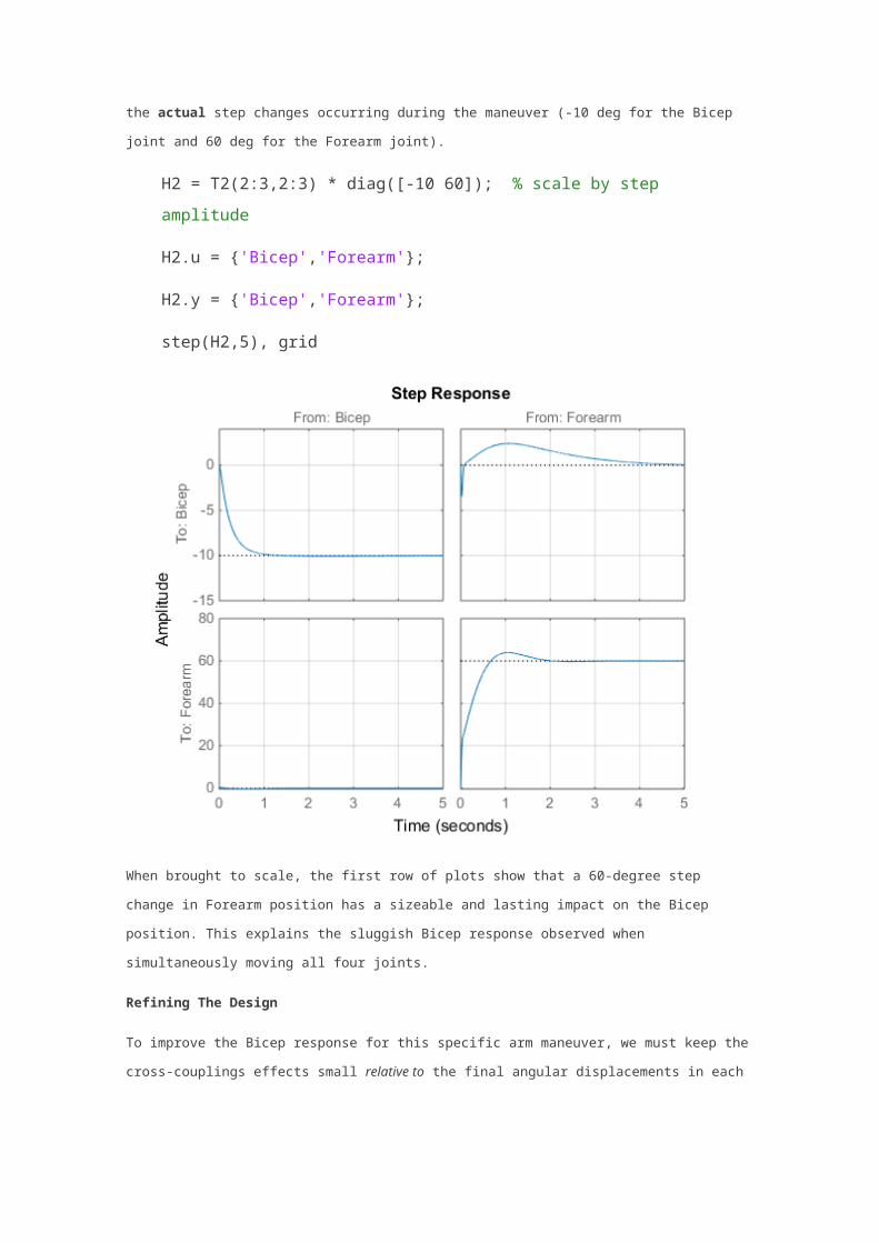
actual step changes occurring during the maneuver (-10 deg for the Bicep joint and 60 deg for the

Forearm joint).

H2 = T2(2:3,2:3) * diag([-10 60]); % scale by step

amplitude

H2.u = {'Bicep','Forearm'};

H2.y = {'Bicep','Forearm'};

step(H2,5), grid

When brought to scale, the first row of plots show that a 60-degree step change in Forearm position has a

sizeable and lasting impact on the Bicep position. This explains the sluggish Bicep response observed

when simultaneously moving all four joints.

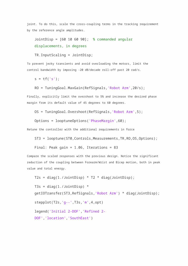
Refining The Design

To improve the Bicep response for this specific arm maneuver, we must keep the cross-couplings effects

small relative to the final angular displacements in each joint. To do this, scale the cross-coupling terms in

the tracking requirement by the reference angle amplitudes.

JointDisp = [60 10 60 90]; % commanded angular

displacements, in degrees

TR.InputScaling = JointDisp;

To prevent jerky transients and avoid overloading the motors, limit the control bandwidth by imposing -20

dB/decade roll-off past 20 rad/s.

s = tf('s');

RO = TuningGoal.MaxGain(RefSignals,'Robot Arm',20/s);

Finally, explicitly limit the overshoot to 5% and increase the desired phase margin from its default value of

45 degrees to 60 degrees.

OS = TuningGoal.Overshoot(RefSignals,'Robot Arm',5);

Options = looptuneOptions('PhaseMargin',60);

Retune the controller with the additional requirements in force

ST3 = looptune(ST0,Controls,Measurements,TR,RO,OS,Options);

Final: Peak gain = 1.06, Iterations = 83

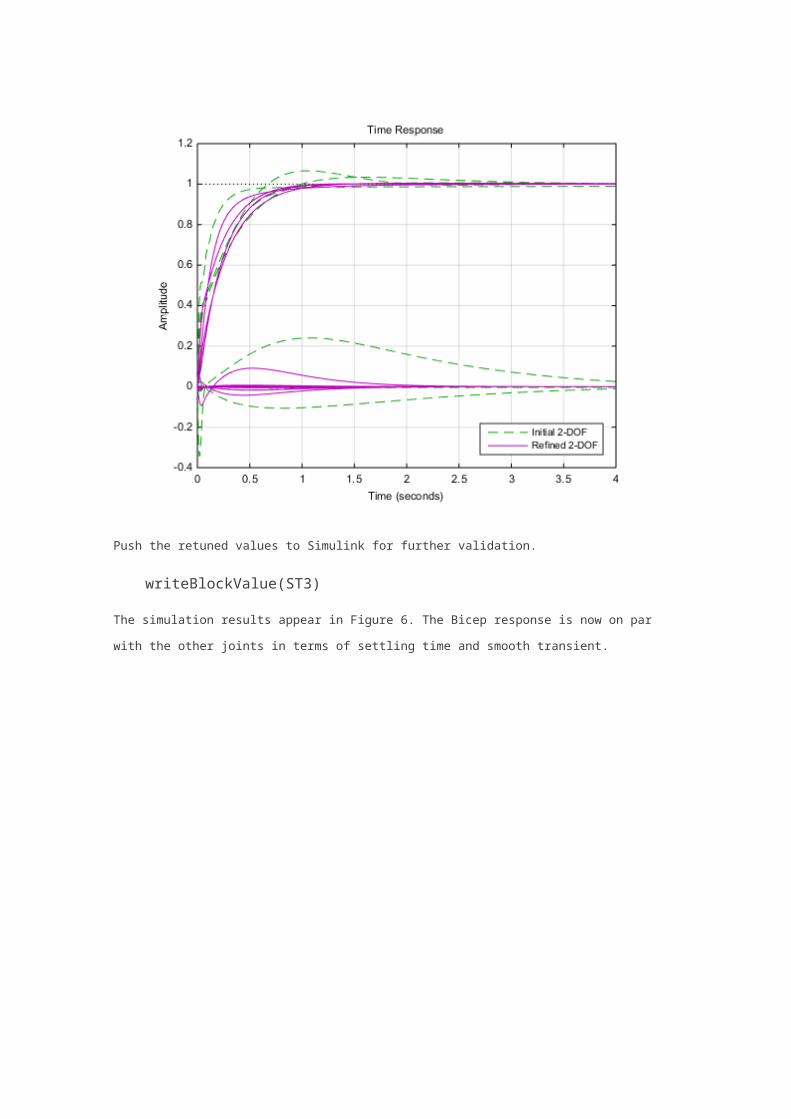
Compare the scaled responses with the previous design. Notice the significant reduction of the coupling

between Forearm/Wrist and Bicep motion, both in peak value and total energy.

T2s = diag(1./JointDisp) * T2 * diag(JointDisp);

T3s = diag(1./JointDisp) *

getIOTransfer(ST3,RefSignals,'Robot Arm') * diag(JointDisp);

stepplot(T2s,'g--',T3s,'m',4,opt)

legend('Initial 2-DOF','Refined 2-

DOF','location','SouthEast')

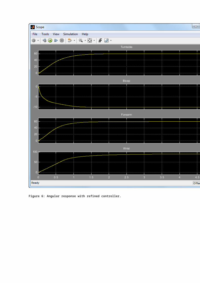
Push the retuned values to Simulink for further validation.

writeBlockValue(ST3)

The simulation results appear in Figure 6. The Bicep response is now on par with the other joints in terms

of settling time and smooth transient.

Figure 6: Angular response with refined controller.

Arduino + Matlab/Simulink: controlador PIDJorge García Tíscar

Jueves, 21 de julio de 2011

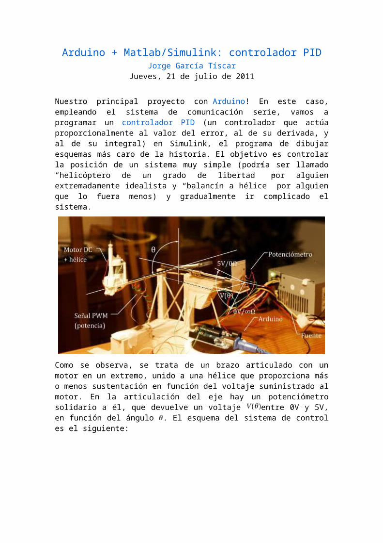
Nuestro principal proyecto con Arduino! En este caso, empleando el sistema de comunicación serie, vamos a programar un controlador PID (un controlador que actúa proporcionalmente al valor del error, al de su derivada, y al de su integral) en Simulink, el programa de dibujar esquemas más caro de la historia. El objetivo es controlar la posición de un sistema muy simple (podría ser llamado “helicóptero de un grado de libertad” por alguien extremadamente idealista y “balancín a hélice” por alguien que lo fuera menos) y gradualmente ir complicado el sistema.

Como se observa, se trata de un brazo articulado con un motor en un extremo, unido a una hélice que proporciona más o menos sustentación en función del voltaje suministrado al motor. En la articulación del eje hay un potenciómetro solidario a él, que devuelve un voltaje entre 0V y 5V, en función del ángulo . El esquema del sistema de control es el siguiente:

De esta manera tenemos definida la variable de salida (posición del eje: voltaje transmitido por el potenciómetro) y la variable de control (sustentación de la hélice: voltaje proporcionado al motor). Nos falta pues un bucle de control (que programaremos en Simulink), una variable de entrada y una interfaz física.

Interfaz física: Arduino + circuito de potencia PWM

Tal y como se explica en una entrada anterior, el Arduino es incapaz por sí mismo de aportar el amperaje que necesita el motor, por lo que emplearemos un circuito de potencia consistente en un transistor MOSFET.

El microcontrolador enviará a la puerta del transistor una señal PWM, y por tanto esta misma señal PWM pero de potencia será la que reciba el motor. La representación de este montaje será la siguente:

Esta es toda la parte física del problema: la planta que vamos a controlar, la variable de salida (ángulo del eje), la variable de control (potencia al motor) y el montaje que hemos realizado con el Arduino. A continuación la parte de código, tanto de Arduino como de Simulink/Matlab.

Arduino: lectura y escritura de variables físicas

En primer lugar, el código del Arduino debe ser capaz  de (1) leer del potenciómetro, (2) enviarlo como dato a través del puerto serie, (3) recibir el dato de potencia necesaria al motor y (4) escribir dicho dato en la salida analógica como señal PWM. Hay que tener en cuenta que el conversor devuelve un valor entre 0 y 1024, que mapeamos a 0 y 255 para poder enviarlo como un solo bit unsigned.

1

2

3

int out = 0;

byte in = 0;

byte pinOut = 10;

4

5

6

7

8

9

10

11

12

13

14

15

16

17

18

19

20

21

22

23

24

25

26

27

void setup() {

  // inicializar puerto serie

  Serial.begin(9600);

  // preparar output

  pinMode(pinOut, OUTPUT);

}

void loop() {

  // leer del pin A0 como

  out = analogRead(A0);

  // escalar para obtener formato uint8

  out = map(out, 0, 1023, 0, 255);

  // enviar en base 10 en ASCII

  Serial.write(out);

  // leer del serie si hay datos

  if(Serial.available()){

    in = Serial.read();

    // escribir en el pin 10

    analogWrite(pinOut, in);

  }

  // esperar para estabilizar el conversor

  delay(20);

}

Simulink: referencia y bucle de control

Por otra parte, nuestro programa de Simulink debe recibir este dato de a través del puerto serie, compararlo con una referencia que controlaremos nosotros con un slider en la propia interfaz gráfica de Simulink, y, mediante un controlador PID, determinar la señal de control (potencia al motor) necesaria. Después debe enviarla a través del puerto serie en formato uint8, unsigned integer de 8 bits, que toma valores entre 0 y 255, ideales para la función analogWrite() de Arduino (click para ampliar):

Dentro del bloque PID, se pueden editar los parámetros P, I y D, siendo los últimos que hemos empleado P = 0.26 , I = 0.9, D = 0.04 y una discretización de 10 ms. Otro dato a tener en cuenta es que la transmisión serie se hace en formato uint8, pero las operaciones se hacen en formato double, de ahí los conversores. Las ganancias son de valor 5/1024 para pasar la señal a voltios reales.

A continuación, un vídeo de todo el sistema en funcionamiento (esta es una de las primeras pruebas, con otros parámetros del PID sin optimizar todavía):

Se puede observar cómo mediante el slider ajustamos la referencia (señal lila). El sistema, ajustando la señal de potencia entregada al motor (señal azul) va ajustando el ángulo del eje hasta conseguir que el voltaje del potenciómetro (señal amarilla) coincida con la referencia que le hemos indicado. Incluso, a pesar de estar en una primera fase de pruebas, se observa que es capaz de resistir a Salva perturbaciones.

Matlab: postproceso de los datos recogidos

Si nos fijamos en el programa de Simulink anterior, se puede observar que no sólo se presentan en el visor las tres señales, sino que además se guardan en el espacio de trabajo de Matlab. Esto nos permite, a posteriori, procesar los resultados del proceso de control como queramos: identificación de sistemas, exportación a Excel… en este caso, nos contentamos con emplear la genial función externa savefigure() para obtener un gráfico vectorial PDF:

1

2

3

4

5

6

7

8

9

10

11

12

%% Preparar la figura

f = figure('Name','Captura');

axis([0 length(ref_out) 0 5.1])

grid on

xlabel('Medida (-)')

ylabel('Voltaje (V)')

title('Captura de voltaje en tiempo real con Arduino')

hold all

%% Tratamiento

pos_out = pos_out(:);

pid_out = pid_out(:);

x = linspace(0,length(ref_out),length(ref_out));

13

14

15

16

17

18

19

20

21

22

%% Limpiar figura y dibujar

cla

plot(x,pid_out,'Color',[0.6,0.6,0.6],'LineWidth',2)

plot(x,ref_out,x,pos_out,'LineWidth',2)

legend('Control','Referencia','Posición','Location','Best');

%% Salvar el gráfico

savefigure('resultado','s',[4.5 3],'po','-dpdf')

Ejecutando este código tras haber realizado una prueba del sistema, hemos obtenido el siguiente gráfico, que a pesar de ser originalmente un gráfico vectorial PDF, hemos rasterizado como PNG para poder representarlo aquí:

Se observa en este caso que el motor requiere mucho menos voltaje (en gris) debido a que se trata de uno más potente que el inicial y que el sistema presenta todavía una sobreoscilación (overshoot) en la señal de salida (en rojo) cuando la señal de referencia (en verde) presenta una subida escalón, cosa que esperamos corregir en futuras versiones. El siguiente desarrollo programado es realizar un control con dos grados de libertad en lugar de uno… not because it’s easy, but because it’s hard!