digital outcrop models: applications of terrestrial ... · digital outcrop models: applications of...

JOURNAL OF SEDIMENTARY RESEARCH, VOL. 75, NO. 2, MARCH, 2005, P. 166–176Copyright q 2005, SEPM (Society for Sedimentary Geology) 1527-1404/05/075-166/$03.00 DOI 10.2110/jsr.2005.013

DIGITAL OUTCROP MODELS: APPLICATIONS OF TERRESTRIAL SCANNING LIDAR TECHNOLOGY INSTRATIGRAPHIC MODELING

J.A. BELLIAN, C. KERANS, AND D.C. JENNETTEBureau of Economic Geology, John A. and Katherine G. Jackson School of Geosciences, The University of Texas at Austin, Austin, Texas, U.S.A.

ABSTRACT: Laser ranging is extremely accurate and efficient. Terres-trial scanning lidar (light detection and ranging) applied to outcropstratigraphic mapping enables researchers to capture laser range dataat a rate of thousands of individual X, Y, Z and laser-intensity pointsper second. These data, in conjunction with complementary remotelyand directly sampled data, are used to conduct high-precision faciescharacterization and to construct 3D geological computer models. Out-crop data are presented here to explain our workflow and to discussthe construction of rock-based 3D Digital Outcrop Models (DOMs).Reproducibility and quantification are the drivers of this methodology.High-resolution terrestrial lidar acquisition, processing, interpretation,and visualization are discussed and applied to mapping of geologicalsurfaces in three dimensions. Laser-generated models offer scientistsan unprecedented visualization medium in a quantitative 3D arena.Applications of this technology include constructing and visualizingcomplex 3D Earth models from outcrops for improved reservoir mod-eling, flow simulation in hydrocarbon and aquifer systems, and prop-erty modeling to constrain forward seismic modeling.

INTRODUCTION

Laser ranging has been used extensively by a variety of remote sensinggroups. For decades the National Aeronautics and Space Administration(NASA), for instance, has used laser ranging to track satellites. The termlidar (light detection and ranging) first appeared in geoscience literature inthe 1960s (Schuster 1970 and references therein) in relation to atmosphericaerosol studies. Lidar (also known as ladar, optical radar, or laser radar)has grown in popularity since the 1960s and is now used in a variety ofscientific, law enforcement, surveying, and construction applications. Re-gardless of the application, all lidar instruments operate on the same pre-mise. A laser pulse leaves the gun, travels to a remote target, bounces offthe target, and returns to a detector. This two-way travel time is dividedin half and multiplied by the speed of light to calculate an accurate Zdistance. Position in X and Y positions are calculated on the basis of theposition of the gun (or laser-deflecting mirrors) when the laser pulse leavesthe instrument. The precision of these lidar instruments has increased fromseveral meters to a few millimeters since its initial application in the early1960s (Noll 2003).

Lidar is like sonar or radar except laser light, instead of sound waves orradio waves, is used to measure distance with extreme precision. Manymodern scanners use ‘‘time of flight’’ to measure distance on the basis ofthe average speed of light in air. This measurement varies with air density,but because the speed of light is so great, these perturbations are very smallfor distances less than several kilometers. Other instruments use phase rec-ognition to augment this technique for increased precision; however, thismethod is associated with an increase in data volume, which is undesirablewhen constructing models on the scale of several to hundreds of kilometers(and several hundred million points). Commercially available scanning li-dar instruments are capable of surveying many thousands to hundreds ofthousands of X, Y, Z points per second; some also have the capability ofrecording laser intensity (I) at each X, Y position. Faster and longer-rangeinstruments (. 1,000 m) are available but have large power requirementsand are not portable enough for a single user to backpack into remote fieldsettings. Small battery-operated units initially targeted for civil engineeringand facilities operations applications are publicly available and are ideal

for remote field settings. For this study, a compact terrestrial scanner ca-pable of collecting 2000 X, Y, Z, and I points per second was used on thebasis of instrument portability and 1 km range capability (Fig. 1). This unituses a 1500 nm infrared Class One laser that is eye safe in all operatingconditions.

We have applied recent developments in scanning lidar technology tooutcrop stratigraphic modeling and developed a method to produce high-accuracy DOMs. These DOMs serve as the 3D template or backbone forreservoir characterization geocellular models. A discussion of techniquesused in acquisition, processing, interpretation, and, most importantly, in-tegration is presented, along with examples of contributions lidar has madeto outcrop studies thus far.

Traditional digital elevation models, or DEMs, differ from DOMs in thatoutcrop models require frequent use of multiple-Z values for accurate rep-resentation of outcrop faces, especially in highly rugose outcrop settings.Rugosity complicates processing because traditional, regularly spaced gridfiles, the kind most, if not all, DEMs are constructed from, do not containfull 3D coordinate information. The structure of a grid file has a start andend point defined, then a long list of attributes (in this case Z is the attri-bute) assumed to be at regularly spaced intervals throughout the file withno single position having more than one attribute associated with it. Inother words a sphere could not be accurately represented using a regulargrid file like that mentioned above. DOMs are generated from triangulatedirregular networks of points (TIN) or commonly known as triangular meshfiles. These files have explicit points defined in 3D space (X, Y, and Z)with the option to add attributes such as color, laser intensity, processedpixels, etc. to each random point or node.

To create an accurate 3D representation of outcrop strata having complexreentrants and overhangs, high-resolution laser data must be acquired frommultiple perspectives and combined with traditional stratigraphic field mea-surements. This process allows the observer to track stratigraphic horizonsin 3D and extract more precise 3D shape information from the outcrop.Through digital manipulation of the model, the viewer can scrutinize theoutcrop from virtually any perspective. Obstructions can be digitally re-moved (vegetation, buildings, etc.), previously inaccessible vertical wallscan be inspected with high-resolution 3D photographic texture, correlationthrough mountains and across valleys can be made, and these observationscan all be combined on a three-dimensional interactive display (immersive3D visualization environment or even a laptop). Since the data are all in3D, behind the outcrop cores, ground penetrating radar, seismic and/or coreplug information can be readily imported to improve the quantitative geo-logical model.

With the many benefits high-resolution lidar offers, there are challeng-es as well. Scanning lidar can generate multigigabyte data sets in a fewhours. These large data sets become difficult to manipulate interactivelyand interpret. We offer some solutions to this problem, as well as visu-alization techniques, textural mapping of laser intensity and photographsusing VRML (virtual reality modeling language), geological interpreta-tion techniques, and multicomponent classification of data. Digitizinggeological features on a DOM or 3D point cloud preserves the data di-rectly in the digital realm (from the outcrop), reducing potential manualor mechanical transfer errors, and directly preserves three-dimensionalityof the actual rocks. Any lidar data can be registered to GPS coordinates,but careful attention must be paid to the level of accuracy of the GPSbeing recorded. High-resolution lidar (, 1cm point spacing) is far more

167DIGITAL OUTCROP MODELS

FIG. 1.—A typical field setup in Patagonia inearly 2002. All equipment was transported in abackpack by a single person (picture courtesy ofJeremy Willson, Shell Oil). Lithium Ion batterieshave helped reduce battery weight to 1,540grams (3.4 pounds) per approximately 2 hours ofcontinuous scan time.

FIG. 2.—Point-cloud image from the mouth ofVictorio Canyon, Texas. Note the region ofblack not captured from a single vantage-pointscan. The image has been rotated down slightlyto show these data shadows (arrows). The grayscale assigned to each pixel is laser intensityresponse.

accurate in three dimensions than nearly all GPS currently available tothe public. Lidar has also been proven to be valuable for other forms ofspatial information, such as capturing and archiving national monumentsand historic sites (Louden 2002), as well as mining, urban planning, andcivil engineering. Later we will illustrate a workflow for integrating moretraditional geological field data with high-resolution lidar to produce aDOM at the reservoir scale.

PREVIOUS WORK

Lidar is by no means the first method that has been used to gatherquantitative stratigraphic data—measuring stratigraphic columns is themost obvious example. These classic data are critical to understanding one-dimensional (Kerans and Tinker 1997; Read et al. 1995) stacking patterns,but they are also used in concert to compare lateral continuities to quantify

168 J.A. BELLIAN ET AL.

FIG. 3.—Workflow diagram from upper left to lower right. Black arrows indicate flow direction, red arrows indicate feedback, like the subtask of converting measuredstratigraphic sections into directional pseudo-wells in GOCAD. Steps 2, 3B, and 4 are conducted in Polyworks. Lower-left image (Step 3A a) shows optimized surfacemodel, with full-resolution (Step 3A b) laser intensity image below it. Step 3A a is completed using optimization code (freeware ‘‘Qslim’’) and ER Mapper. Step 3A cillustrates a perspective view of photographic texture blended with laser intensity (50% opacity-blend). Upper-right image (Step 4) illustrates the subtask loop used totransfer measured stratigraphic sections into pseudo-well objects in GOCAD for vertical and horizontal facies distribution. The final objective is a composite of all thevarious parts in modeling software such as GOCAD (Step 5) to construct a rock-driven geocellular 3D DOM. There are multiple software packages to perform all of thesefunctions; the names listed here are for reference to the text.

stratigraphy along 2D/3D outcrops. Photographs have helped in correlationfrom measured sections, as well as in other uses of technology, such asGPS. Several research groups have been involved in taking outcrop datadirectly into the digital realm since the late 1990s. Various techniques havebeen explored, such as the use of (1) photogrammetry to build outcrop-based seismic models (Stafleu et al. 1996), (2) real-time kinematic globalpositioning systems or RTK GPS to trace bedding surfaces manually inconjunction with nonscanning (single-shot) laser surveying instruments(McCormick and Grotzinger 2001; McCormick et al. 2000), (3) single-shotlaser surveying of outcrop erosion profiles as a proxy for seismic imped-ance (Bracco Gartner and Schlager 1997a, 1997b, 1999; Bracco Gartner2000), (4) ground-penetrating radar (McMechan et al. 1998; Loucks et al.2001; Hammon et al. 2002; McMechan et al. 2002; Dunn et al. 2003), (5)photogrammetry and ground-penetrating radar combined (Pringle et al.2001), (6) ‘‘photorealistic mapping’’ (Xu et al. 1999; Xu 2000; Xu et al.

2000), or (7) lidar in conjunction with ground penetrating radar (Wizevichet al. 1999; Bhattacharya et al. 2000; Bellian et al. 2004). Each of thesetechniques has its strengths and weaknesses for fast, accurate capture ofstratal geometries and relationships. The fundamental difference in ourmethod is improved edge detection and model optimization (Bellian et al.2002; Bellian et al. 2003a; Bellian et al. 2003b; Jennette and Bellian 2003;Kerans et al. 2003; Bellian et al. 2004; Janson et al. 2004). Previous meth-ods have focused on taking low-resolution models and draping or texturinghigh-resolution images on these data to fill in detail of a low-resolutionsurface model. Our method from inception has focused on gathering high-resolution lidar data and generating geological models directly from thesedata. Photo-drape or other image-attribute data are then later applied to theoptimized version of this data set, preserving only the critical data requiredto accurately represent edges and curves while reducing unnecessary pointsin less rugose regions.


FIG. 4.—A) Digital elevation model (DEM) of the Franklin Mountains, Texas, with B) an orthorectified air photo C) draped over the DEM. Note inset image highlightingimage distortion in steeply dipping regions. Also note red and white radio tower plastered to the side of the mountain. These data were downloaded from the USGSNational Map seamless-data distribution service (http://seamless.usgs.gov).

INSTRUMENTATION

An Optech Laser Imaging ILRIS 3D terrestrial (ground-based) scanninglidar instrument was chosen for its 1 km range, palm-type interface, andlight weight. All data from the ground-based lidar surveys were processed

on a standard laptop computer with at least a gigahertz processor speed, 1gigabyte of RAM and Innovmetric Incorporated’s Polyworks CAD (Com-puter Aided Design) software. There are several manufacturers of lidarinstrumentation similar to ILRIS and other CAD software options publicly


TABLE 1.—Vertices and texture coordinates for Figure 6.

X Y Z

Figure 6A:Vertex

12345

0.000.001.001.000.50

0.001.000.001.000.50

1.001.001.001.001.50

Texture coordinate (Figure 6B with above vertices)

12345

0.000.001.001.000.50

0.001.000.001.000.50

Figure 6C:Vertex

12345

0.000.001.001.000.50

0.001.000.001.000.50

1.001.001.001.001.50

Texture coordinate

12345

0.000.001.001.000.75

0.001.000.001.000.75

Figure 6A is the shape model constructed from the vertices only from this table. Figure 6B has the texturecoordinates added to the vertices, allowing the flat-image Figure 6A (2D Original image file) to drape correctlyover the pyramid shape. Figure 6C vertices and texture coordinates are shifted off of center (see vertex andtexture coordinate 5). Note vertices in image 6A, B, and C are identical, only the texture coordinates areshifted (from X 5 0.5, Y 5 0.5 to X 5 0.75, and Y 5 0.75 for vertex 5).

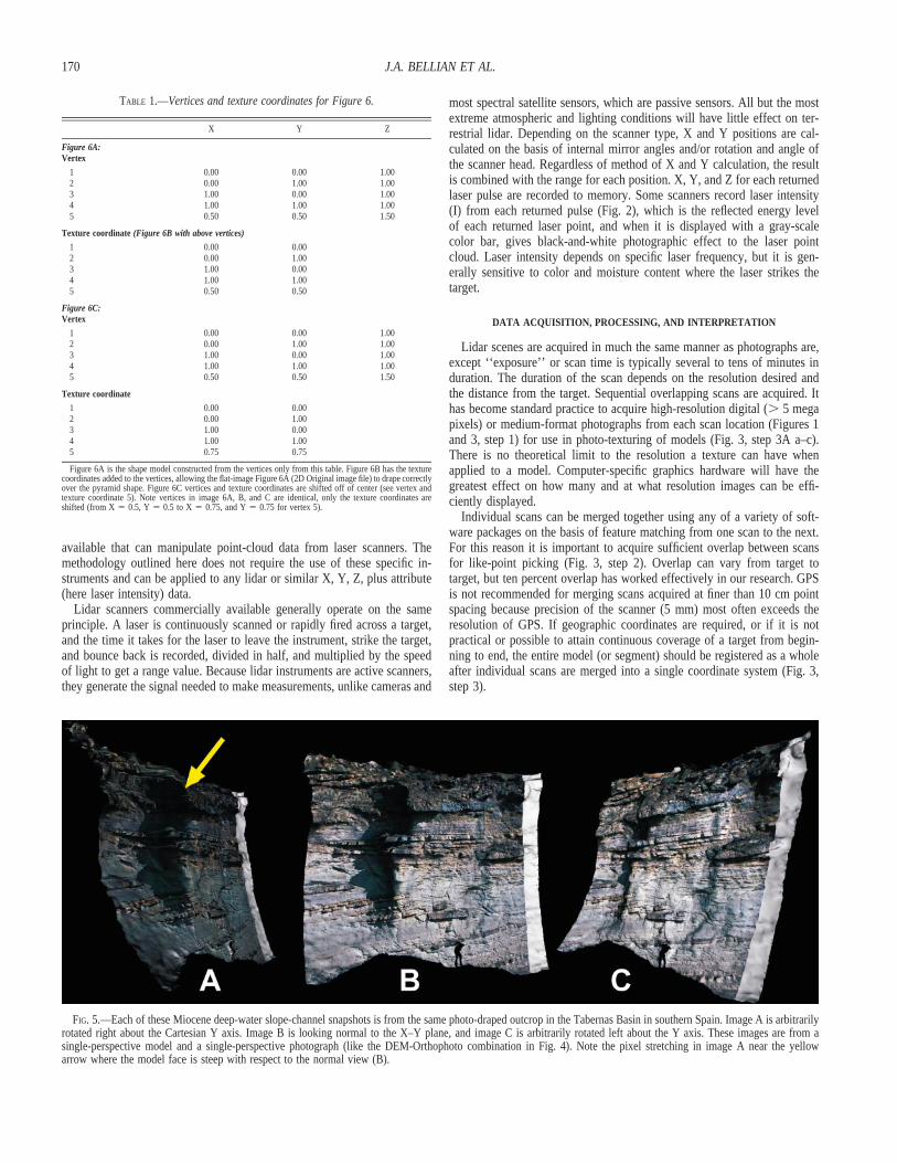
FIG. 5.—Each of these Miocene deep-water slope-channel snapshots is from the same photo-draped outcrop in the Tabernas Basin in southern Spain. Image A is arbitrarilyrotated right about the Cartesian Y axis. Image B is looking normal to the X–Y plane, and image C is arbitrarily rotated left about the Y axis. These images are from asingle-perspective model and a single-perspective photograph (like the DEM-Orthophoto combination in Fig. 4). Note the pixel stretching in image A near the yellowarrow where the model face is steep with respect to the normal view (B).

available that can manipulate point-cloud data from laser scanners. Themethodology outlined here does not require the use of these specific in-struments and can be applied to any lidar or similar X, Y, Z, plus attribute(here laser intensity) data.

Lidar scanners commercially available generally operate on the sameprinciple. A laser is continuously scanned or rapidly fired across a target,and the time it takes for the laser to leave the instrument, strike the target,and bounce back is recorded, divided in half, and multiplied by the speedof light to get a range value. Because lidar instruments are active scanners,they generate the signal needed to make measurements, unlike cameras and

most spectral satellite sensors, which are passive sensors. All but the mostextreme atmospheric and lighting conditions will have little effect on ter-restrial lidar. Depending on the scanner type, X and Y positions are cal-culated on the basis of internal mirror angles and/or rotation and angle ofthe scanner head. Regardless of method of X and Y calculation, the resultis combined with the range for each position. X, Y, and Z for each returnedlaser pulse are recorded to memory. Some scanners record laser intensity(I) from each returned pulse (Fig. 2), which is the reflected energy levelof each returned laser point, and when it is displayed with a gray-scalecolor bar, gives black-and-white photographic effect to the laser pointcloud. Laser intensity depends on specific laser frequency, but it is gen-erally sensitive to color and moisture content where the laser strikes thetarget.

DATA ACQUISITION, PROCESSING, AND INTERPRETATION

Lidar scenes are acquired in much the same manner as photographs are,except ‘‘exposure’’ or scan time is typically several to tens of minutes induration. The duration of the scan depends on the resolution desired andthe distance from the target. Sequential overlapping scans are acquired. Ithas become standard practice to acquire high-resolution digital (. 5 megapixels) or medium-format photographs from each scan location (Figures 1and 3, step 1) for use in photo-texturing of models (Fig. 3, step 3A a–c).There is no theoretical limit to the resolution a texture can have whenapplied to a model. Computer-specific graphics hardware will have thegreatest effect on how many and at what resolution images can be effi-ciently displayed.

Individual scans can be merged together using any of a variety of soft-ware packages on the basis of feature matching from one scan to the next.For this reason it is important to acquire sufficient overlap between scansfor like-point picking (Fig. 3, step 2). Overlap can vary from target totarget, but ten percent overlap has worked effectively in our research. GPSis not recommended for merging scans acquired at finer than 10 cm pointspacing because precision of the scanner (5 mm) most often exceeds theresolution of GPS. If geographic coordinates are required, or if it is notpractical or possible to attain continuous coverage of a target from begin-ning to end, the entire model (or segment) should be registered as a wholeafter individual scans are merged into a single coordinate system (Fig. 3,step 3).


FIG. 6.—VRML-rendered images in this figureare in pairs. Pair A shows original 3Dnontextured object in plan view (left) andperspective view (right). Pair B shows quadrantmatching texture plan view (left) and perspectiveview (right). Pair C shows a shift of the centertexture coordinate (texture coordinate 5 for 6Cin Table 1) in plan view (left) and perspectiveview (right). Note poor registration of centerpoint in Pair C causes stretch distortion inquadrants 1 and 2 in C and smashing of circlesin quadrants 3 and 4. Even in Pair B where theregistration is correct, there is still noticeablepixel stretch.

Each time the instrument is moved, including rotation about the sta-tionary tripod, the scanner is automatically reset to a new Cartesian co-ordinate origin in 3D space. Thus even two consecutive scans, althoughseemingly from the same location, will have coordinate origins differentfrom one another. If the two files were opened simultaneously in oneimage window, each would plot on top of the other with X, Y, Z coor-dinates equal to 0, 0, 0, typically in the lower-left corner of the imagewindow, just as two photographs from a photo pan would open if notstitched together first. In order to merge multiple scans in 3D, a trans-formation matrix is solved by repositioning one scan with reference toanother. Software such as Polyworks will perform this transformationsemiautomatically on the basis of a few user-defined control points fromoverlap regions of the scans being merged (Fig. 3, red spheres in step 2).The point cloud is then reprojected using the matrix solution into thenewly transformed coordinate space. This process is repeated for allscans; quality of the final merge depends on the method used and theoriginal data resolution. Depending on the software used, methods mayvary, although it is important to understand to what level of precision thesoftware is capable of merging scans. Cumulative merge error can be-

come significant if the scans are not merged to a sufficient level of cer-tainty (in Polyworks the iteration is set to an error tolerance of 1027).Unwanted points are deleted after the final merge and quality check arecomplete.

After data are satisfactorily merged, the workflow bifurcates into twobranches (Fig. 3, step 3)—the first is a stratigraphic interpretation and mea-sured section positioning (performed in Polyworks), and the second is thebuilding of a virtual outcrop model of optimized surfaces that can be dis-played in geocellular modeling packages such as GOCAD.

Measured sections and other relevant data (sample locations, faults, geo-graphic markers, etc.) are added to the merged 3D point cloud manuallyby matching features on the point cloud to those known from fieldwork orthat are georeferenced with GPS. These data can be used to calibrate geo-logical interpretation between the model and the outcrop. Stratigraphic ho-rizons are digitized directly on the 3D point cloud in a manner similar tothat used when mapping seismic horizons along a random slice through aseismic volume and exported to modeling software as ASCII or DXF for-mat 3D line files. The measured sections are converted to directional wellsposted along this random slice and likewise exported to modeling software.


FIG. 7.—Miocene deep-water slope-channelarchitecture digitized directly on the DOM anddisplayed as a VRML model. This file can beinteractively interrogated and compared with un-interpreted models, as well as interactively viewhand-sample images and photomicrographs forpetrographic studies or even import and overlayseismic snapshots to inspect viability ofinterpretation based on this model.

Interpretations and sections are converted into GOCAD objects, from whichhorizons and facies distributions are constructed (outlined later).

Although commercial software has recently become available for someof these processes, computer code was developed in house to give us great-er control over the data (John Andrews, Bureau of Economic Geology,personal communication, 2003). This code incorporates an excellent pre-existing, quadric-based, surface-reduction program (Garland 1999) to op-timize TINs while preserving original shape. Our first step extracts the full-resolution intensity point cloud (X, Y, I) and converts it into a tagged imagefile format (TIFF) file to be applied later as a texture to the correspondingoptimized surface model. The range data (X, Y, Z) are also extracted andassembled into a triangulated mesh (Fig. 3, step 3A a). This mesh uses theTIN optimization code ‘‘Qslim 2.0’’ (Garland 1999) to reduce the numberof triangles generated from each laser point cloud. Texture coordinates(explained below) are calculated for each point cloud run through this pro-cessing routine and exported to any of a number of output formats. Forconstruction of the DOM, we export optimized TINs and correspondingtexture coordinates in GOCAD ‘‘Tsurf’’ format (Fig. 3A, step 5) and asvirtual reality modeling language (VRML) object files. VRML files areextremely versatile multiplatform, interactive objects that can be viewed inactive or passive stereo and combined with other VRML files and variousother data types for versatile visualization format (Thurmond et al. 2004).VRML viewing applications are web-browser-type plug-in files or stand-alone software for cross-platform 3D model viewing. Many viewers areavailable for free (http://www.ca.com/cosmo/) and are gaining popularitywithin the geoscience community.

PHOTO-TEXTURED MODEL

Digital photo-draping of ‘‘3D’’ surfaces has been performed for nearlya decade. The United States Geological Survey is one organization that has

posted free DEMs (Fig. 4A) and orthophotographs (Fig. 4B) of nearly theentire United States and several other parts of the world (http://seamless.usgs.gov) at various resolutions. The DEMs downloaded from the Internetcan be co-rendered or textured in x, y space with corresponding orthopho-tographs (or any other imagery) to produce a color, photo-textured topo-graphic model (Fig. 4C). DEMs are typically digitized from topographicmaps or acquired from airborne or orbital sources (e.g., airborne radar,airborne lidar, and/or satellite). These methods preclude the option of gath-ering multiple z values at any single x, y position, as can be done with aground-based scanner. For this reason, most DEM grid files are a digitallist of z values (because they are unique at each x, y) with a startingcoordinate, number of columns and rows, and unit spacing and do not needto explicitly specify every point as an X, Y, Z location. The list helps limitthe number of bits required to store and process these data. Thus ‘‘3D’’models generated from these single-perspective data are actually more like‘‘2½D’’ because they do not contain information from multiple perspec-tives. For instance, overhanging objects such as bridges or steep rock out-crops are not visible or they become severely distorted with a single-per-spective data set. Likewise, being able to see inside a cave or building isnot an option because there is no way to account for this information in aregularly spaced grid file. Areas not imaged are called data shadows andare often represented as holes in the model, or they are covered over withan interpolated surface, like a window being shut or a cloth draped over achair limiting the level of detail that can be studied. This situation makesthe use of DEMs limited in detailed outcrop analysis, especially when res-olutions are commonly two orders of magnitude too coarse for detailedfacies mapping (0.5 to 3 m point spacing) and steeply dipping outcropfaces are obscured by perspective-driven data shadows (inset in Fig. 4C).The red-and-white radio tower in Figure 4C appears to have been deflatedand draped over the outcrop, and a smeared texture of the photograph can


FIG. 8.—DOM of the Permian VictorioCanyon toe-of-slope carbonate-fan complex.Pseudo-wells can be seen along 3D tan-coloredcanyon walls, with vertical pseudo-well colorscorresponding to specific facies. The horizonprojected across the canyon is an oolitic fan-complex isocore map, with depositional directionto the lower right (northeast). Red is zerothickness, with yellow through light-purplerepresenting 1 to 5 m. The scale of this model is1.5 3 2.5 km.

be observed because of the flat photograph being deformed to fit the steeptopography of the Franklin Mountains DEM. The radio tower was not largeenough or lucky enough to be recognized by the regularly spaced DEMgrid samples (10 m point spacing). When a photograph and a DEM ac-quired from a single perspective are used, pixel-stretch artifacts like thoseof the inset in Figure 4C are unavoidable. The x and y coordinates of theflat photograph are digitally matched to the x, y coordinates of the DEMand, thus, the z value (elevation in this case) of the DEM is pushed throughthe image to cover the entire DEM shape. In steep regions of the DEMonly a few photograph pixels are available to fill an area larger than thephotograph pixels can physically cover; the pixels are thus smeared orstretched to fill the available space. The amount of pixel stretch dependson the variability of the model surface and how similar the angle of ac-quisition of the DEM is to the angle of acquisition of the image beingdraped (here an aerial photograph).

In order to assemble a ‘‘3D’’ DOM, a series of ‘‘2½-D’’ textured scansare merged together and rendered simultaneously as a single shape object.This can be done in many modeling software packages, but most operatesimilarly, in this aspect, to VRML objects. That is, objects are constructedfrom a series of points and connected together as a triangulated mesh. Eachvertex of the mesh has an associated texture coordinate that maps eachtriangle vertex to a specific pixel on the texture image. The pyramids inFigure 6 were constructed from the vertices and texture coordinates in

Table 1. Each triangle of the model may have an unlimited number ofimage pixels within it. Shape models generated from optimized large datasets (many millions of points) are more likely to accurately represent theobject being modeled than models created from more coarsely spaced ran-dom laser points.

Texture coordinates are values assigned to each vertex as a percentageof the texture image in X and Y directions. For example, if there are fivenodes defining four corners and one in the center that outlines four triangles(Fig. 6A), each node is assigned a texture coordinate between 0 and 1.00(or 0 to 100%). Beginning in the upper-left corner, X and Y are definedas 0, 0. The lower-right corner texture coordinates are X 5 1.00 (or 100%)and Y 5 1.00 (or 100%). Likewise, the lower-left corner and upper-rightcorner coordinates are X 5 0 and Y 5 1.00 and X 5 1 and Y 5 0,respectively. The texture coordinates for the center node are X 5 0.50, Y5 0.50. In this way, regardless of the pixel density of the image file (orimage dpi), the corresponding percentage of the image will be displayedbetween the correct nodes of each triangle (Fig. 6B). To illustrate this point,we changed the central texture coordinate in Figure 6C from the correctlocation, 0.50, 0.50, to an offset, incorrect location, 0.75, 0.75 (Table 1);the number of pixels on the left side of center node would thus be com-pressed, with the remaining pixels stretched out on the right side of thecenter node (Fig. 6C) to fill triangles one and two. This distortion in Figure6C was induced by poor image registration to the model.


FIG. 9.—DOM facies interpolation projected on Victorio Canyon walls. Quality of the facies distribution function for the entire model can be examined and checkedagainst the outcrop and calibrated if needed.

FIG. 10.—ER Mapper UnsupervisedClassification analyzing slope and laser intensitydata from Victorio Canyon. The combination ofthese two attributes for this Permian toe-of-slopedebrite and turbidite complex enhances thinwackestone beds cut out or plowed by debrisflows in the green (yellow arrows). This exampleshows one utility of being able to combinemultiple data types in n-dimensional space.


Even with near-perfect image registration to the model (well-matchedtexture coordinates to image pixels), distortion will always be present ontilted surfaces. The closer to each triangle normal (vector perpendicular tothe triangle face) the texture image acquisition angle is, the less distortionthere will be within that triangle (Fig. 9B). Upon close inspection of Figure6B, the circles in each quadrant are stretched slightly from the original 2Dimage file in Figure 6. In order to eliminate this effect, four separate pic-tures would be required for Figure 6B, one from each normal to eachnumbered face. The same concept holds true for any textured model (Fig.5). It is not reasonable to expect to acquire a photograph from every pos-sible model normal, especially if the model has many millions of faces. Itis critical to understand this concept if interpreting high-resolution strati-graphic models from textured surface models. It is proposed here that geo-logical interpretation should be performed on the original point cloud dataand not the resultant textured model whenever possible to reduce inherentpixel-stretch errors affecting geological interpretation.

Images used as texture do not have to be photographs. Any image canbe a texture—for example, interpreted photographs from previous work ora sample-location grid over a photograph (Fig. 7). The use of texture co-ordinates is an excellent way to display interpreted results in 3D at variousresolutions. Images can be readily exchanged by changing the link to theimage file, as long as the new image has the exact same field of view.

CONSTRUCTION OF A 3D GEOCELLULAR MODEL

Up to this point we have focused on gathering data, interpreting stratig-raphy, creating surfaces, and adding textures for visualization. These makeup the skeleton from which a spatially correct 3D geocellular model isconstructed. The stratigraphic line files digitized along the outcrop facefrom the merged, unfiltered laser data are used to create 3D horizons de-fining top and base of each stratal unit. These horizons become the bound-ing surfaces for the grid cells of the model. Outcrop selection can thereforeinfluence the outcome of the model. The more three-dimensional the out-crop, the better the model will be able to represent the actual geology.Victorio Canyon, in the Permian Basin of West Texas, is a good exampleof outcrop three-dimensionality. Both sides of the canyon and side canyonswere laser scanned and interpreted, and then stratal surfaces were projectedacross the canyons (Fig. 8). Interpretations can be projected onto any ran-dom plane to extrapolate true-strike and true-dip perspectives of any out-crop.

Pseudo-wells derived from measured stratigraphic sections are used todistribute facies vertically and horizontally within the stratal units (Fig. 9).This facies realization can be compared to field observations and adjust thedistribution function used for the facies model. This stochastic methodincreases realistic property distribution in 3D. Once a facies model is built,velocity values can be distributed throughout the model using the faciesmodel as proxy for velocity distribution. From the velocity model, syntheticseismic sections are calculated for the DOM (Janson et al. 2004).

MULTICOMPONENT CLASSIFICATION

Multicomponent image classification has been applied to satellite-imageanalysis and, to a lesser extent, seismic-attribute processing to extract spe-cific attributes on multiple data sets simultaneously. A summary of mul-ticomponent data processing can be found in Vincent (1997). The classi-fication in Figure 10 was performed using ER Mapper image-processingsoftware. This technique compares various image types with one another,assuming co-registration of the sample nodes. Each node is assigned nattributes based on n textures to be compared. Mathematical trends areextracted from these data in n-dimensional space, where n is the numberof attributes or textures in this case. A new attribute (classification) isgenerated from the processed textures. Trends not visually apparent to theobserver in either of the two input textures individually can be enhanced

in the new classification. This direction in outcrop research can lead to newunderstanding of depositional systems and advance quantitative outcropgeology.

An example of this type of data visualization in outcrop compares twoattributes, laser intensity and outcrop slope. These two components werecombined to make a new classified image texture. The data were classifiedusing the ER Mapper unsupervised classification function, choosing sevenarbitrary bins with which to categorize the data (Fig. 10). Note the bluehighlighted areas, which correspond to thin-bedded carbonate wackestonesthat were incised/plowed by thick-bedded carbonate debris flows. This isa simplistic example of what can be done with a more robust suite of datasuch as multispectral or even hyperspectral data for deterministic remotemapping. Research in this area is ongoing.

DISCUSSION

Terrestrial scanning lidar provides us with the ability to make rapid,quantitative measurements of a study area with modest topographic relief(vertical cliffs , 1 km high) down to centimeter resolution. The ability ofthe user to digitally inspect in 3D stratigraphic correlations, trace faultplanes, and project geology across canyons and through mountains, as wellas to combine multiple images for multidimensional analysis, makes lidara unique and extremely valuable tool for outcrop geologists. Lidar is fastbecoming a critical tool for offering a step change in current field methods.Digital outcrop models, or DOM’s, offer the following advances:

● With the aid of lidar we can now gather essential three-dimensional pointclouds and make geological interpretations directly on them.

● Oblique outcrop geometries can now be projected onto a specific planeefficiently enough to offer true strike or true dip perspectives, preservingscale and geometry.

● Data extracted from these quantitative geological DOMs can be readilyincorporated into reservoir models with tools available to both the ge-ologist and the engineer.

● Field trips can now begin at the office to prepare participants for whatthey are going to see, highlight key observations to note, and previewpotential safety hazards.

● Field geologists can use these data to more accurately estimate budgetsfor field expeditions.

● Areas traditionally inaccessible can be brought back into the office,classroom, or visualization laboratory.

● Integration of multiple data types into a single model will not only helpgeologists preview, study, and document field observations, but also re-tain and understand information captured visible and invisible to thehuman eye.

Finally, it is important to recognize that lidar is a tool with which wecan improve our current field methods and quantify the observations ge-ologists make. This tool is in no way meant to take the place of first-handobservation of geology. For this there is no substitute.

ACKNOWLEDGMENTS

We would like to thank the sponsors of the Bureau of Economic Geology Res-ervoir Characterization Research Laboratory (RCRL) Industrial Associates program(please refer to http://www.beg.utexas.edu/indassoc/rcrl/index.htm for a complete listof current sponsors) at the Jackson School of Geosciences at The University of Texasat Austin who supplied the critical funding for this project and the ongoing questto advance rock-based geological modeling. Publication authorized by the Director,Bureau of Economic Geology. A special thanks goes to the University of Texas atAustin Geology Foundation at the Jackson School of Geosciences for assistance inprint charges for this manuscript.

REFERENCES

BELLIAN, J.A., JENNETTE, D.C., KERANS, C., GIBEAUT, J., ANDREWS, J., YSSLDYK, B., AND LARUE,D., 2002, 3-Dimensional digital outcrop data collection and analysis using eye-safe laser


(LIDAR) technology (abstract): American Association of Petroleum Geologists, AnnualMeeting, Programs with Abstracts, Houston, March 10–13.

BELLIAN, J.A., KERANS, C., AND PLAYTON, T., 2003a, Textural mapping with lidar and real-timekinematic GPS on the flow-unit scale: an example from the Pipe Creek Early Albian rudistbuildup, Central Texas (abstract): American Association of Petroleum Geologists, AnnualMeeting, Programs with Abstracts, Salt Lake City, May 11–14.

BELLIAN, J.A., JENNETTE, D.C., AND GUTIERREZ, R., 2003b, Dual-purpose geologic analysis usingairborne and ground-based lidar, coastal Southern California: quantitative 3-D characteriza-tion of modern coastal erosion and ancient reservoir architecture (abstract): American As-sociation of Petroleum Geologists, Annual Meeting, Programs with Abstracts, Salt LakeCity, May 11–14.

BELLIAN, J.A., KERANS, C., JANSON, X., AND PLAYTON, T., 2004, Digital Outcrop Models: Amer-ican Association of Petroleum Geologists, Annual Meeting, Extended Abstracts, El Paso,March 15–18.

BHATTACHARYA, J.P., XU, X., AIKEN, L.V.C., AND WILLIS, B.J., 2000, Using GPS and lasers tomap subtle tectonic structures that control positions of reservoir sandstones in foreland basins(abstract): American Association of Petroleum Geologists, Annual Meeting, New Orleans,April 16–19.

BRACCO GARTNER, G.L., 2000, High resolution impedance models of outcrops and their appli-cations in seismic interpretation: Amsterdam, Vrije Universiteit, Sedimentology and MarineGeology Section, 144 p.

BRACCO GARTNER, G.L., AND SCHLAGER, W., 1997a, Topographic slope as an estimator of acous-tic impedance: Sedimentary Geology, v. 112, p. 1–6.

BRACCO GARTNER, G.L., AND SCHLAGER, W., 1997b, Quantification of topography using a laser-transit system: Journal of Sedimentary Research, v. 67, p. 987–989.

BRACCO GARTNER, G.L., AND SCHLAGER, W., 1999, Discriminating between onlap and lithologicinterfingering in seismic models of outcrops: American Association of Petroleum Geologists,Bulletin, v. 83, no. 6, p. 952–971.

DUNN, P., VAN WAGONER, J.C., AND DEFFENBAUGH, M., 2003, Hierarchical, self-affine fluvialsand body shapes from ancient and modern settings: American Association of PetroleumGeologists, Annual Meeting, Extended Abstracts, Salt Lake City, May 11–14.

GARLAND, M., 1999, Quadric-based polygonal surface simplification [unpublished Ph.D. dis-sertation]: Pittsburgh, Carnegie Mellon University, 210 p.

HAMMON, W.S., ZENG, X., CORBEANU, R.M., AND MCMECHAN, G.A., 2002, Estimation of thespatial distribution of fluid permeability from surface and tomographic GPR data and core,with a 2-D example from the Ferron Sandstone, Utah: Geophysics, v. 67, no. 5, p. 1505–1515.

JANSON, X., KERANS, C., BELLIAN, J.A., PLAYTON, T., AND FITCHEN, W.M., 2004, Outcrop-based3-D synthetic seismic of Early Permian deep water carbonate deposits, Victorio Canyon,West Texas (abstract): American Association of Petroleum Geologists, Annual Meeting,Programs with Abstracts, Dallas, April 18–21.

JENNETTE, D., AND BELLIAN, J.A., 2003, 3-D digital characterization and visualization of thesolitary channel complex, Tabernas Basin, southern Spain (abstract): American Associationof Petroleum Geologists, International Meeting, Programs with Abstracts, Barcelona, Spain,September 21–23.

KERANS, C., AND TINKER, S., 1997, Sequence Stratigraphy and Characterization of CarbonateReservoirs: SEPM, Short Course, no. 40, 130 p.

KERANS, C., BELLIAN, J.A., AND PLAYTON, T., 2003, 3-D modeling of deepwater carbonate out-crops using laser technology (lidar) (abstract): American Association of Petroleum Geolo-gists, Annual Meeting, Programs with Abstracts, Salt Lake City, May 11–14.

LOUCKS, R.G., MESCHNER, P., AND MCMECHAN, G., 2001, Characterizing the three-dimensionalarchitecture of a coalesced, collapsed-paleocave system in the Lower Ordovician, Ellenbur-

ger Group by integrating ground-penetrating radar, shallow-core, and outcrop data (abstract):American Association of Petroleum Geologists, Annual Meeting, Denver, Colorado, June3–6, p. 121.

LOUDEN, E.I., 2002, Mapping Miss Liberty: Geospatial Solutions, September, p. 38–41.MCCORMICK, D.S., AND GROTZINGER, J.P., 2001, Digital mapping of Neoproterozoic thrombolite-

grainstone facies architecture in Namibia; analog for intrasalt reservoirs in South Oman saltbasin: American Association of Petroleum Geologists, Annual Meeting, Expanded Abstracts,June 3–6.

MCCORMICK, D.S. THURMOND., J.B., GROTZINGER, J.P., AND FLEMING, R.J., 2000, Creating a three-dimensional model of clinoforms in the upper San Andres Formation, Last Chance Canyon,New Mexico (abstract): American Association of Petroleum Geologists, Annual Meeting,New Orleans, April 16–19.

MCMECHAN, G.A., LOUCKS, R.G., ZENG, X., AND MESCHER, P., 1998, Ground penetrating radarimaging of a collapsed paleocave system in the Ellenburger Dolomite, central Texas: Journalof Applied Geophysics, v. 39, no. 1, p. 1–10.

MCMECHAN, G.A., LOUCKS, R.G., MESCHER, P., AND ZENG, X., 2002, Characterization of a co-alesced, collapsed paleocave reservoir analog using GPR and well-core data: Geophysics,v. 67, p. 1148–1158.

NOLL, C., web site digital publication accessed April 2003, http://ilrs.gsfc.nasa.gov/docs/slrover.pdf NASA Goddard Space Flight Center (http://www.gsfc.nasa.gov), Greenbelt,Maryland.

PRINGLE, J.K., CLARK, J.D., WESTERMAN, A.R., STANBROOK, D.A., GARDINER, A.R., AND MORGAN,B.E., 2001, Animations in geology: visualising the Earth: Journal of the Virtual ExplorerOnline, v. 3, p. 51–55.

READ, J.F., KERANS, C., WEBER, L.J., SARG, R., AND WRIGHT, F.M., 1995, Milankovitch Sea-Level Changes, Cycles, and Reservoirs on Carbonate Platforms in Greenhouse and Ice-houseWorlds: SEPM, Short Course no. 35, 147 p.

SCHUSTER, B.G., 1970, Detection of tropospheric and stratospheric aerosol layers by opticalradar (lidar): Journal of Geophysical Research, v. 75, p. 3123–3132.

STAFLEU, J., SCHLAGER, W., EVERTS, A.J.W., KENTER, J.A.M., BLOMMERS, G., AND VAN-VOORDEN,A., 1996, Outcrop topography as a proxy of acoustic impedance in synthetic seismograms:Geophysics, v. 61, p. 1779–1788.

THURMOND, J.B., DRZEWIECKI, P.A., AND XU, X., 2004, Building simple multiscale visualizationsof outcrop geology using Virtual Reality Modeling Language (VRML): Unpublished work.

VINCENT, R.K., 1997, Fundamentals of Geological and Environmental Remote Sensing: NewJersey, Prentice Hall, 366 p.

WIZEVICH, M., MCMECHAN, G., AIKEN, C., CORBEANU, R., ZENG, X., BALDE, M., XU, X., FORSTER,C., AND SNELGROVE, S., 1999, A multi-disciplinary approach to reservoir (and aquifer) char-acterization and flow simulation; integration of a 3-D GPR, GPS/laser rangefinder survey,outcrop, and borehole data (abstract): Geological Society of America, Northeastern Section,34th Annual Meeting, Providence, Rhode Island.

XU, X., 2000, Three-dimensional virtual geology; photorealistic outcrops, and their acquisition,visualization and analysis [unpublished Ph.D. dissertation]: The University of Texas at Dal-las, 170 p.

XU, X., AIKEN, C.L., AND NIELSEN, K.C., 1999, Real time and the virtual outcrop improvegeological field mapping: Eos, Transactions, American Geophysical Union, v. 80, no. 29,p. 317–322.

XU, X., AIKEN, C.L., BHATTACHARYA, J.P., CORBEANU, R.,M., NIELSEN, K.C., MCMECHAN, G.A.,AND ABDELSALAM, M.G., 2000, Creating virtual 3-D outcrop: The Leading Edge, v.19, no. 2,p. 197–202.

Received 17 June 2004; accepted 19 October 2004.

digital outcrop models: applications of terrestrial ... · digital outcrop models: applications of...

Documents