digital image processing (cs/ece 545) lecture filters...
TRANSCRIPT

Digital Image Processing (CS/ECE 545) Lecture 4: Filters (Part 2)
& Edges and Contours
Prof Emmanuel Agu
Computer Science Dept.Worcester Polytechnic Institute (WPI)

Recall: Applying Linear Filters: Convolution
1. Move filter matrix H overimage such that H(0,0) coincides with current imageposition (u,v)
For each image position I(u,v): 2. Multiply all filter coefficients H(i,j)with corresponding pixelI(u + i, v + j)
3. Sum up results and store sum in corresponding positionin new image I’(u, v)
Stated formally:
RH is set of all pixels Covered by filter.For 3x3 filter, this is:
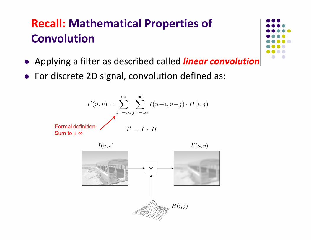
Recall: Mathematical Properties of Convolution
Applying a filter as described called linear convolution For discrete 2D signal, convolution defined as:

Recall: Properties of Convolution
Commutativity
Linearity
(notice)
Associativity
Same result if we convolve image with filter or vice versa
If image multiplied by scalarResult multiplied by same scalar
If 2 images added and convolveresult with a kernel H, Same result if we each imageis convolved individually + added
Order of filter application irrelevantAny order, same result

Properties of Convolution
Separability
If a kernel H can be separated into multiple smaller kernels Applying smaller kernels H1 H2 … HN H one by one
computationally cheaper than apply 1 large kernel H
ComputationallyMore expensive
ComputationallyCheaper

Separability in x and y
Sometimes we can separate a kernel into “vertical” and “horizontal” components
Consider the kernels

Complexity of x/y Separable Kernels
What is the number of operations for 3 x 5 kernel HAns: 15wh
What is the number of operations for Hx followed by Hy?Ans: 3wh + 5wh = 8wh

Complexity of x/y Separable Kernels
What is the number of operations for 3 x 5 kernel HAns: 15wh
What is the number of operations for Hx followed by Hy?Ans: 3wh + 5wh = 8wh
What about M x M kernel?O(M2) – no separability (M2wh operations, grows quadratically!)O(M2) – with separability (2Mwh operations, grows linearly!)

Gaussian Kernel
1D
2D

Separability of 2D Gaussian
2D gaussian is just product of 1D gaussians:
Separable!

Separability of 2D Gaussian
Consequently, convolution with a gaussian is separable
Where G is the 2D discrete gaussian kernel; Gx is “horizontal” and Gy is “vertical” 1D discrete Gaussian kernels

Impulse (or Dirac) Function
In discrete 2D case, impulse function defined as:
Impulse function on image? A white pixel at origin, on black background

Impulse (or Dirac) Function
Impulse function neutral under convolution (no effect) Convolving an image using impulse function as filter = image

Impulse (or Dirac) Function
Reverse case? Apply filter H to impulse function Using fact that convolution is commutative
Result is the filter H

Noise While taking picture (during capture), noise may occur Noise? Errors, degradations in pixel values Examples of causes: Focus blurring Blurring due to camera motion
Additive model for noise:
Removing noise called Image Restoration Image restoration can be done in: Spatial domain, or Frequency domain

Types of Noise
Type of noise determines best types of filters for removing it!! Salt and pepper noise: Randomly scattered black + white pixels Also called impulse noise, shot noise or binary noise Caused by sudden sharp disturbance
Courtesy Allasdair McAndrews

Types of Noise Gaussian Noise: idealized form of white noise added to
image, normally distributed Speckle Noise: pixel values multiplied by random noise
Courtesy Allasdair McAndrews

Types of Noise
Periodic Noise: caused by disturbances of a periodic nature
Salt and pepper, gaussian and speckle noise can be cleaned using spatial filters
Periodic noise can be cleaned using frequency domain filtering (later) Courtesy
Allasdair McAndrews

Non‐Linear Filters Linear filters blurs all image structures points, edges and
lines, reduction of image quality (bad!) Linear filters thus not used a lot for removing noise
Sharpedge
SharpThinLine
BlurredEdgeResults
BlurredThinLineResults
Apply LinearFilter

Using Linear Filter to Remove Noise?
Example: Using linear filter to clean salt and pepper noise just causes smearing (not clean removal)
Try non‐linear filters? Courtesy Allasdair McAndrews

Non‐Linear Filters Pixels in filter range combined by some non‐linear function Simplest examples of nonlinear filters: Min and Max filters
Beforefiltering
Afterfiltering
Step Edge(shifted to right)
NarrowPulse(removed)
Linear Ramp(shifted to right)
Effect ofMinimum filter

Non‐Linear Filters
Original Image withSalt-and-pepper noise
Minimum filter removesbright spots (maxima) andwidens dark image structures
Maximum filter (opposite effect):Removes dark spots (minima) andwidens bright image structures

Median Filter
Much better at removing noise and keeping the structures
Sort pixel values within filter region Replace filter “hot spot” pixel
with median of sorted values

Illustration: Effects of Median Filter
Isolated pixels are eliminated
A step edge isunchanged
A corner is rounded off
Thin lines are eliminated

Effects of Median Filter
Original Image withSalt-and-pepper noise
Linear filter removes some ofthe noise, but not completely.Smears noise
Median filter salt-and-pepper noiseand keeps image structures largelyintact. But also creates small spotsof flat intensity, that affect sharpness
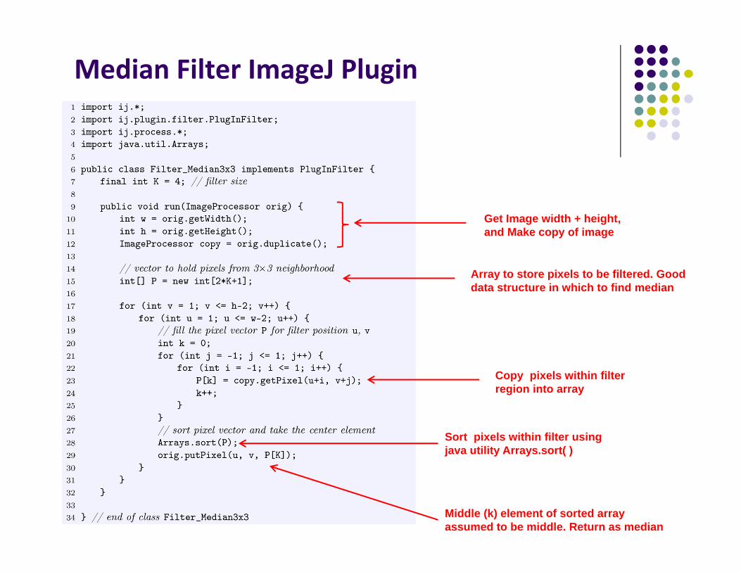
Median Filter ImageJ Plugin
Get Image width + height,and Make copy of image
Array to store pixels to be filtered. Gooddata structure in which to find median
Copy pixels within filter region into array
Sort pixels within filter usingjava utility Arrays.sort( )
Middle (k) element of sorted array assumed to be middle. Return as median

Weighted Median Filter
Color assigned by median filter determined by colors of “the majority” of pixels within the filter region
Considered robust since single high or low value cannot influence result (unlike linear average)
Median filter assigns weights (number of “votes”) to filter positions
To compute result, each pixel value within filter region is inserted W(i,j) times to create extended pixel vector
Extended pixel vector then sorted and median returned

Weighted Median Filter
Weight matrix
Pixels within filter region
Insert each pixel within filter region W(I,j) times into extended pixel vector
Sort extended pixel vector and return median
Note: assigning weight to center pixel larger than sum of all other pixel weights inhibits any filter effect (center pixel always carries majority)!!

Weighted Median Filter More formally, extended pixel vector defined as
For example, following weight matrix yields extended pixel vector of length 15 (sum of weights)
Weighting can be applied to non‐rectangular filters Example: cross‐shaped median filter may have weights

An Outlier Method of Filtering
Algorithm by Pratt, Ref: Alasdair McAndrew, Page 116 Median filter does sorting per pixel (computationally expensive) Alternate method for removing salt‐and‐pepper noise
Define noisy pixels as outliers (different from neighboring pixels by an amount > D)
Algorithm: Choose threshold value D For given pixel, compare its value p to mean m of 8 neighboring pixels If |p –m| > D, classifiy pixel as noise, otherwise not If pixel is noise, replace its value with m; Otherwise leave its value
unchanged
Method not automatic. Generate multiple images with different values of D, choose the best looking one

Outlier Method Example Effects of choosing different values of D
D value of 0.3 performs best Overall outlier method not as good as median filter
D value too small: removes noise from dark regions
D value too large: removes noise from light regions
Courtesy Allasdair McAndrews

Other Non‐Linear Filters
Any filter operation that is not linear (summation), is considered linear
Min, max and median are simple examples More examples later: Morphological filters (Chapter 10) Corner detection filters (Chapter 8)
Also, filtering shall be discussed in frequency domain
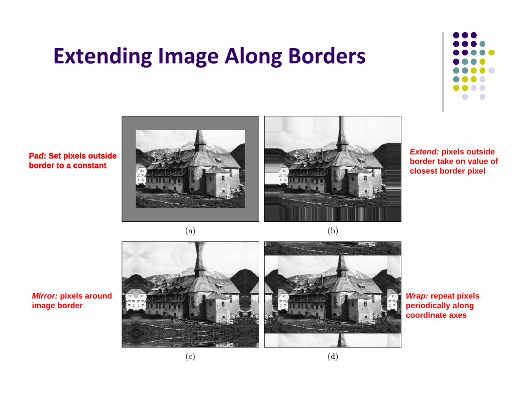
Extending Image Along Borders
Pad: Set pixels outsideborder to a constant
Mirror: pixels aroundimage border
Pad: Set pixels outsideborder to a constant
Wrap: repeat pixels periodically along coordinate axes
Extend: pixels outsideborder take on value ofclosest border pixel

Filter Operations in ImageJ
Linear filters implemented by ImageJ plugin class ij.plugin.filter.Convolver
Has several methods in addition to run( )
Define filter matrix
Create new instance ofConvolver class
Apply filter (Modifies Image I destructively)

Gaussian Filters
ij.plugin.filter.GaussianBlur implements gaussian filter with radius (σ)
Uses separable 1d gaussians
Create new instance ofGaussianBlur class
Blur image ip with gaussian filter of radius r

Non‐Linear Filters
A few non‐linear filters (minimum, maximum and median filters implemented in ij.plugin.filter.RankFilters
Filter region is approximately circular with variable radius
Example usage:

Recall: Linear Filters: Convolution
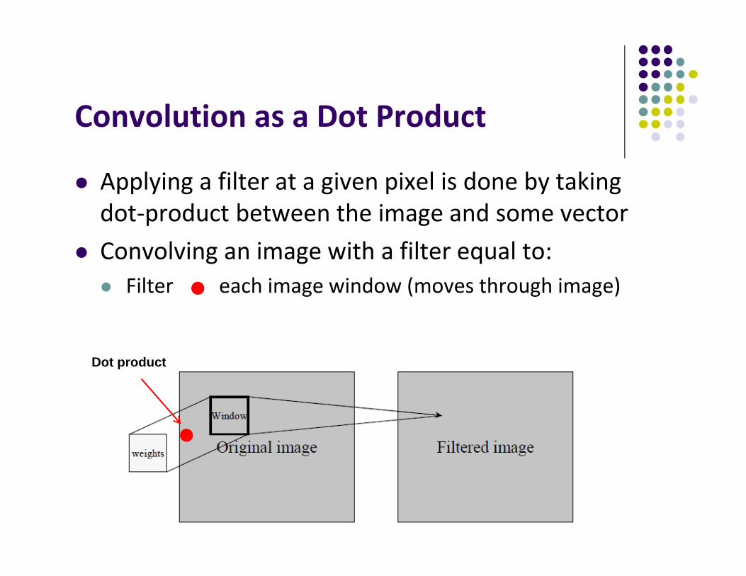
Convolution as a Dot Product
Applying a filter at a given pixel is done by taking dot‐product between the image and some vector
Convolving an image with a filter equal to: Filter each image window (moves through image)
Dot product
Digital Image Processing (CS/ECE 545) Lecture 4: Filters (Part 2)
& Edges and Contours
Prof Emmanuel Agu
Computer Science Dept.Worcester Polytechnic Institute (WPI)

What is an Edge?
Edge? sharp change in brightness (discontinuities) Where do edges occur? Actual edges: Boundaries between objects Sharp change in brightness can also occur within object
Reflectance changes Change in surface orientation Illumination changes. E.g. Cast shadow boundary

Edge Detection Image processing task that finds edges and contours in
images Edges so important that human vision can reconstruct
edge lines

Characteristics of an Edge
Edge: A sharp change in brightness Ideal edge is a step function in some direction

Characteristics of an Edge Real (non‐ideal) edge is a slightly blurred step function Edges can be characterized by high value first derivative
Rising slope causes positive + high value first derivative Falling slope causes negative
+ high value first derivative

Characteristics of an Edge Ideal edge is a step function in certain direction. First derivative of I(x) has a peak at the edge Second derivative of I(x) has a zero crossing at edge
Ideal edge
Real edge
First derivativeshows peak
Second derivativeshows zero crossing

Slopes of Discrete Functions
Left and right slope may not be same Solution? Take average of left and right slope
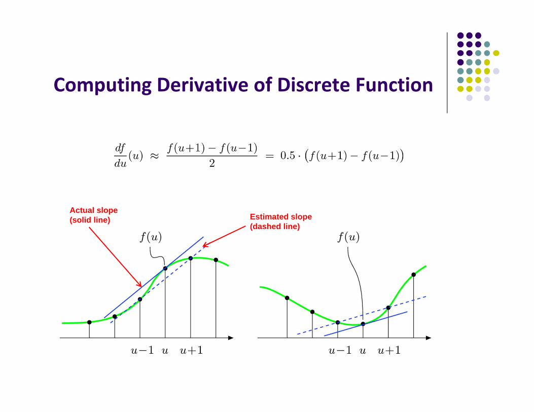
Computing Derivative of Discrete Function
Actual slope (solid line) Estimated slope
(dashed line)

Finite Differences
Forward difference (right slope)
Backward difference (left slope)
Central Difference (average slope)

Definition: Function Gradient
Let f(x,y) be a 2D function Gradient: Vector whose direction is in direction of maximum
rate of change of f and whose magnitude is maximum rate of change of f
Gradient is perpendicular to edge contour

Image Gradient Image is 2D discrete function Image derivatives in horizontal and vertical directions
Image gradient at location (u,v)
Gradient magnitude
Magnitude is invariant under imagerotation, used in edge detection

Derivative Filters
Recall that we can compute derivative of discrete function as
Can we make linear filter that computes central differences
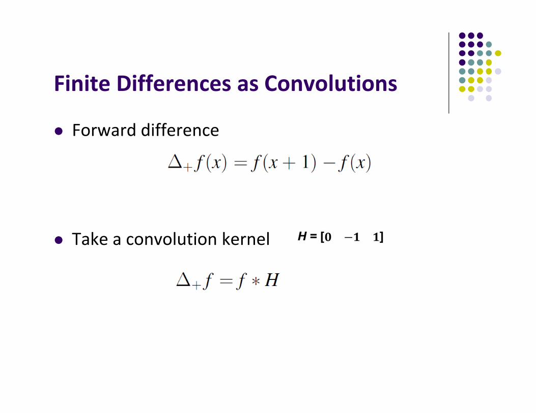
Finite Differences as Convolutions
Forward difference
Take a convolution kernel

Finite Differences as Convolutions
Central difference
Convolution kernel is:
Notice: Derivative kernels sum to zero

x‐Derivative of Image using Central Difference
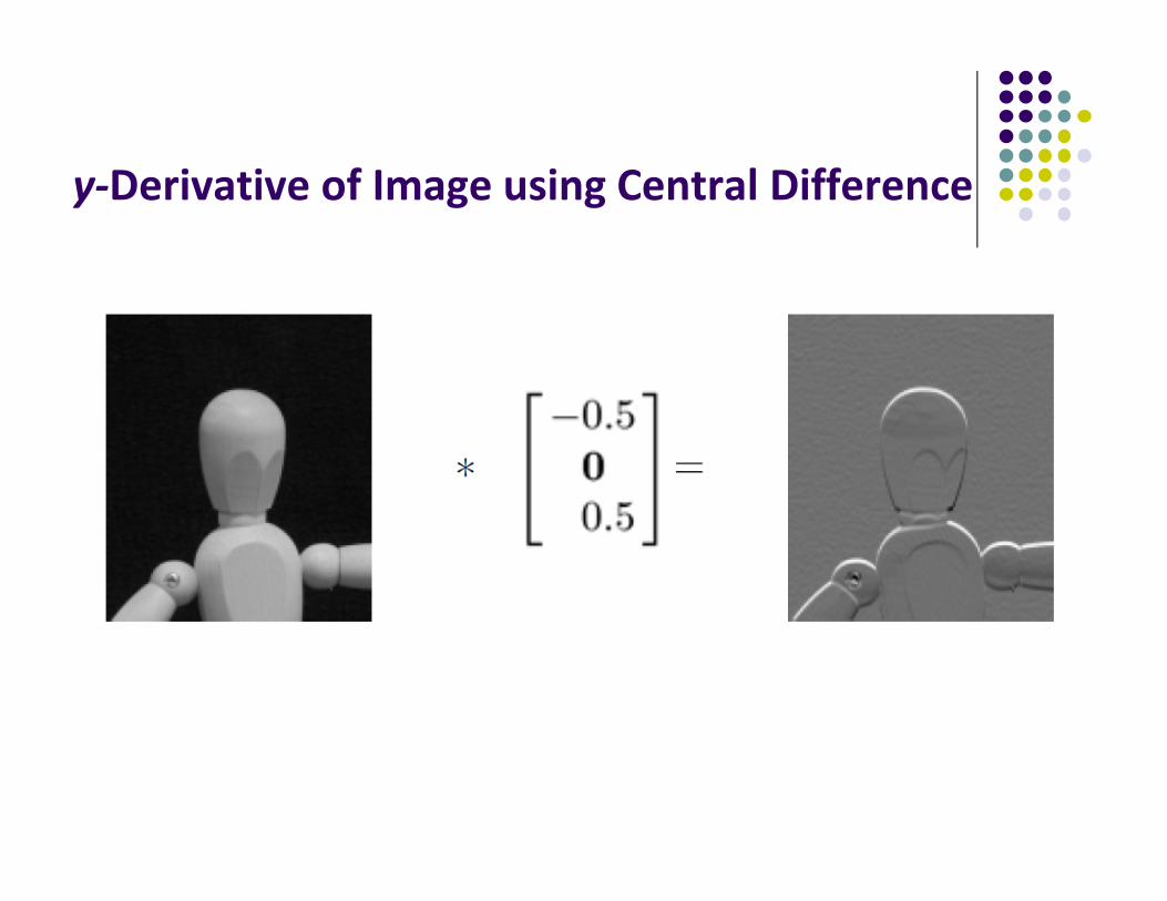
y‐Derivative of Image using Central Difference

Derivative Filters
A syntheticimage
Magnitude ofgradient
Gradient slope in vertical direction
Gradient slope in horizontal direction

Edge Operators
Approximating local gradients in image is basis of many classical edge‐detection operators
Main differences? Type of filter used to estimate gradient components How gradient components are combined
We are typically interested in Local edge direction Local edge magnitude
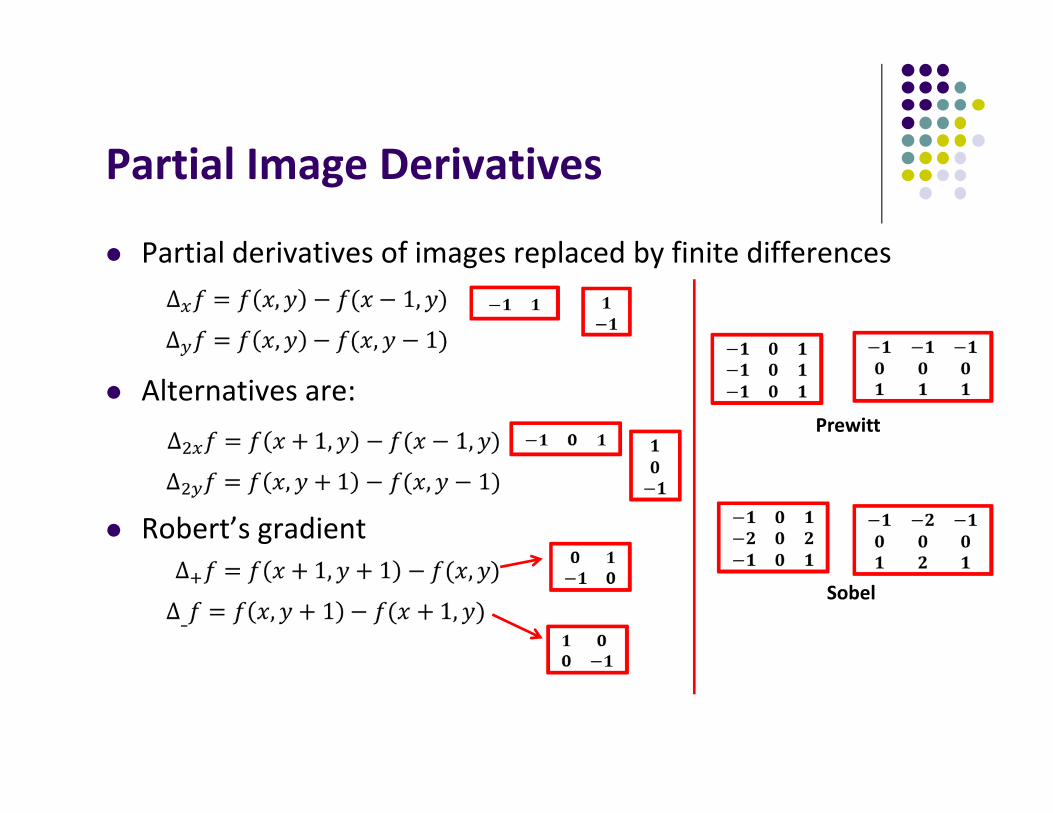
Partial Image Derivatives
Partial derivatives of images replaced by finite differences
Alternatives are:
Robert’s gradient
Prewitt
Sobel

Using Averaging with Derivatives
Finite difference operator is sensitive to noise Derivates more robust if derivative computations are
averaged in a neighborhood Prewitt operator: derivative in x, then average in y
y‐derivative kernel, defined similarly
Average in y direction
Derivative in x direction
Note: Filter kernel is flipped in convolution

Sobel Operator
Similar to Prewitt, but averaging kernel is higher in middle
Average in x direction
Derivative in y directionNote: Filter kernel is flipped in convolution

Prewitt and Sobel Edge Operators
Prewitt Operator
Sobel Operator
Written in separable form

Improved Sobel Filter
Original Sobel filter relatively inaccurate Improved versions proposed by Jahne

Prewitt and Sobel Edge Operators

Scaling Edge Components
Estimates of local gradient components obtained from filter results by appropriate scaling
Scaling factor forPrewitt operator
Scaling factor forSobel operator

Gradient‐Based Edge Detection
Compute image derivatives by convolution
Compute edge gradient magnitude
Compute edge gradient direction
Scaled Filter results
Typical process ofGradient based edge detection

Gradient‐Based Edge Detection
After computing gradient magnitude and orientation then what?
Mark points where gradient magnitude is large wrt neighbors

Non‐Maxima Suppression
Retain a point as an edge point if: Its gradient magnitude is higher than a threshold Its gradient magnitude is a local maxima in gradient direction
Simple thresholding willcompute thick edges

Non‐Maxima Suppression
A maxima occurs at q, if its magnitude is larger than those at p and r

Roberts Edge Operators Estimates directional gradient along 2 image diagonals Edge strength E(u,v): length of vector obtained by adding 2
orthogonal gradient components D1(u,v) and D2(u,v)
Filters for edge components

Roberts Edge Operators Diagonal gradient components produced by 2 Robert filters

Compass Operators
Linear edge filters involve trade‐off
Example: Prewitt and Sobel operators detect edge magnitudes but use only 2 directions (insensitive to orientation)
Solution? Use many filters, each sensitive to narrow range of orientations (compass operators)
Sensitivity to Edge magnitude
Sensitivity toorientation

Compass Operators Edge operators proposed by Kirsh uses 8 filters with
orientations spaced at 45 degrees
Need only to compute 4 filtersSince H4 = - H0, etc

Compass Operators
Edge strength EK at position(u,v) is max of the 8 filters
Strongest‐responding filter also determines edge orientation at a position(u,v)

Edge operators in ImageJ
ImageJ implements Sobel operator Can be invoked via menu Process ‐> Find Edges Also available through method void findEdges( ) for objects of type ImageProcessor

References Wilhelm Burger and Mark J. Burge, Digital Image Processing, Springer, 2008
University of Utah, CS 4640: Image Processing Basics, Spring 2012
Rutgers University, CS 334, Introduction to Imaging and Multimedia, Fall 2012