digital hologram synthesis - zcu.cz · university of west bohemia department of computer science...
TRANSCRIPT
University of West Bohemia
Department of Computer Science and Engineering
Univerzitnı 8
CZ 306 14 Plzen
Czech Republic
Digital Hologram SynthesisState of the art and a concept of doctoral thesis
Ing. Martin Janda
Technical Report No. DCSE/TR-2007-02April, 2007Distribution: public


To my Father

Abstract
The first part of this work summarises the basic knowledge about holography princi-
ples including wave optics and diffraction. The summarised knowledge is consequently
exploited in the second part of this work that regards the methods of digital hologram
synthesis. The synthesis methods were evaluated and compared and the perspective
ones were announced. The perspective synthesis methods served as a starting point
of the further research and the first output of the research is included in the third
part of this work. It is a novel approach to synthesis based on ray casting. The last
part of this work regards the roadmap for the future work.
Prvnı cast prace obsahuje prehled principu holografie a to vcetne zakladu vlnove
optiky a difrakce. Principy jsou nasledne vyuzity v druhe casti prace, ktera obsahuje
prehled znamych postupu pro syntezu digitalnıch hologramu. Syntetizacnı metody
byly vyhodnoceny a porovnany a byly vyhlaseny perspektivnı metody. Ty potom
slouzily jako pocatecnı bod dalsıho vyzkumu jehoz prvnı vysledky jsou uvedeny v
tretı casti prace. Jedna se o novou syntetizacnı metodu zalozenou na metode vrhanı
paprsku. Poslednı cast prace obsahuje popis cılu a smeru dalsıho vyzkumu.


Contents
1 Introduction 3
2 Holography 72.1 Holography physics . . . . . . . . . . . . . . . . . . . . . . . . . . . 7
2.1.1 Wave optics . . . . . . . . . . . . . . . . . . . . . . . . . . . 82.1.2 Interference . . . . . . . . . . . . . . . . . . . . . . . . . . . 102.1.3 Coherence . . . . . . . . . . . . . . . . . . . . . . . . . . . . 122.1.4 Elementary waves . . . . . . . . . . . . . . . . . . . . . . . 152.1.5 Diffraction . . . . . . . . . . . . . . . . . . . . . . . . . . . 162.1.6 Wave propagation . . . . . . . . . . . . . . . . . . . . . . . 21
Huygens-Fresnel principle . . . . . . . . . . . . . . . . . . . 21Fresnel and Fraunhofer approximation . . . . . . . . . . . . 22Diffraction condition and diffraction orders . . . . . . . . . 26Propagation in Angular Spectrum . . . . . . . . . . . . . . 28
2.2 Optical holography . . . . . . . . . . . . . . . . . . . . . . . . . . . 302.2.1 Holography principle . . . . . . . . . . . . . . . . . . . . . . 302.2.2 Inline hologram . . . . . . . . . . . . . . . . . . . . . . . . . 322.2.3 Off axis hologram . . . . . . . . . . . . . . . . . . . . . . . 342.2.4 Additional hologram types . . . . . . . . . . . . . . . . . . 36
Fourier hologram . . . . . . . . . . . . . . . . . . . . . . . . 36Image holograms . . . . . . . . . . . . . . . . . . . . . . . . 37Fraunhofer hologram . . . . . . . . . . . . . . . . . . . . . . 38
2.2.5 Final notes on optical holography . . . . . . . . . . . . . . . 382.3 Digital Holography . . . . . . . . . . . . . . . . . . . . . . . . . . . 38
2.3.1 Digital recording . . . . . . . . . . . . . . . . . . . . . . . . 382.3.2 Digital reproduction . . . . . . . . . . . . . . . . . . . . . . 392.3.3 Hologram synthesis . . . . . . . . . . . . . . . . . . . . . . . 392.3.4 Final notes on digital holography . . . . . . . . . . . . . . . 40
3 Hologram Synthesis Methods 43
i

ii CONTENTS
3.1 Synthesis methods overview . . . . . . . . . . . . . . . . . . . . . . 443.1.1 Diffraction integral evaluation . . . . . . . . . . . . . . . . . 453.1.2 Ray casting . . . . . . . . . . . . . . . . . . . . . . . . . . . 473.1.3 Diffraction between two coplanar planes . . . . . . . . . . . 50
Fresnel approximation . . . . . . . . . . . . . . . . . . . . . 50Angular spectrum propagation . . . . . . . . . . . . . . . . 52
3.1.4 Fourier hologram synthesis . . . . . . . . . . . . . . . . . . 553.1.5 Basis diffraction footprint combination . . . . . . . . . . . . 603.1.6 HPO holograms synthesis methods . . . . . . . . . . . . . . 64
MIT Holovideo Display System . . . . . . . . . . . . . . . . 65Occlusion and shading support . . . . . . . . . . . . . . . . 69Conclusion . . . . . . . . . . . . . . . . . . . . . . . . . . . 70
3.2 Summarisation and evaluation of the methods . . . . . . . . . . . . 70
4 Proposed ray casting synthesis method 734.1 Basic principle . . . . . . . . . . . . . . . . . . . . . . . . . . . . . 73
4.1.1 Summary . . . . . . . . . . . . . . . . . . . . . . . . . . . . 80
5 Summary and Conclusion 815.1 Holography Overview . . . . . . . . . . . . . . . . . . . . . . . . . 815.2 Synthesis methods . . . . . . . . . . . . . . . . . . . . . . . . . . . 82
5.2.1 Diffraction integral evaluation . . . . . . . . . . . . . . . . . 835.2.2 Ray casting . . . . . . . . . . . . . . . . . . . . . . . . . . . 835.2.3 Diffraction between two coplanar planes . . . . . . . . . . . 835.2.4 Fourier hologram specific synthesis . . . . . . . . . . . . . . 845.2.5 Basis diffraction footprint combination . . . . . . . . . . . . 845.2.6 MIT holovideo specific synthesis . . . . . . . . . . . . . . . 855.2.7 Final statement . . . . . . . . . . . . . . . . . . . . . . . . . 85
5.3 Future direction of work . . . . . . . . . . . . . . . . . . . . . . . . 855.3.1 Road Map . . . . . . . . . . . . . . . . . . . . . . . . . . . . 86
Bibliography 89
A Synthesis methods comparison 95
B Research Road Map 97
List of Symbols and Abbreviations 99
List of Figures 100
List of Tables 102
Index 105

Acknowledgements
Work has been supported by these projects:
• 3DTV NoE, grant No. 511568
• LC CPG, MSMT CR project No.LC 06008
1


Chapter 1
Introduction
Display devices are widely used for presenting visual information. For examplepaper made very good service for a very long time until it was replaced with moreuniversal electronic displays quite some time ago. The technology of the electronicdisplays evolved ever since until it reached contemporary quite advanced level.The problem of the paper and inherently the electronic, e.g. LCD liquid crystaldisplay - LCD, cathode ray tube - CRT etc., display is their planarity, whichrestricts the kind of information possible to display without degradation.
The degradation of information is most significant if three dimensional in-formation is displayed on two dimensional display, which is usually managed bysome kind of projection operation, e.g. perspective projection. This projection isunfortunately done in many areas for instance computer aided design - CAD ormultimedia, e.g. games. As a consequence, it is not surprising that many peopleare trying to develop a genuine three dimensional display, which would presentthree dimensional content without degradation.
The genuine three dimensional display would provide three dimensional re-production of arbitrarily complex objects. Such reproduction is more naturalto a human viewer who accordingly understands the displayed data faster andmore reliably. In addition, a true three dimensional display device supports morethan one viewer because each viewer perceives a correct image according to herlocation.
The research on three dimensional display is not a new thing. Some stere-oscopy based techniques have been invented many years ago. The three dimen-sional perception originates form the fact that humans have two eyes slightlyshifted in horizontal direction and therefore they deliver slightly different imagesto the brain which translates the difference into the depth perception. However,the images are again showing the object from one point of view and cannot beobserved from other angles unless some head tracking is involved.
3
4 CHAPTER 1. INTRODUCTION
Another way is a direct extension of the two dimensional display. Instead oflighting up a point of a 2D grid a point of 3D grid is lit up instead. Such displaysare usually referred as volumetric displays. There are many methods of lightingup a point in a space. For instance, there are methods relying on the persistenceof view of a human eye and use fast moving projection screen. Other methodsuses special materials which emits light at the intersection of two laser beamsor a pulsed laser is used to create points of glowing plasma in air. To conclude,the volumetric displays have larger viewing angles but on the contrary the activevolume itself is a constraint and the volumetric displays are incapable of handlingocclusion.
Speaking generally, various three dimensional displays addresses some subset,usually mutually disjunctive, of the aspects of 3D vision but fails to provideothers. Hence, a flawless genuine three dimensional display was not yet developed.There is however one promising technology, which could have remedy for all thementioned problems. This technology is, as one might expect, holography.
Holography is the ultimate displaying technology since it is capable of repro-ducing the whole light field at the microscopic level. The visual perception froma hologram is therefore undistinguishable from a perception of a real object. Thedigital version of holography is especially useful because it allows creating holo-grams of artificial scenes without the quite strict restrictions imposed on opticalholography.
This is maybe a good place to state that not everything called holography isactually holography! Especially the science fiction genre have introduced quitesevere misconceptions about holography. The real holography is actually an anal-ogy of photography. It even uses the same materials for recording as photographydoes. The detailed description of holography can be found in the Chapter 2.
Now one might rightfully ask what is so great about holography. The an-swer is in the word holography itself. It is derivation from two latin words holosand graf which mean approximately the whole recording. Hologram is recordingof both amplitude and phase of a light field emerging from the recorded scene.For this reason holography is so convenient technology for displaying purposes.Holography is able to provide all depth cues, e.g. motion parallax, binocular par-allax, accommodation, occlusion. In this aspect it surpasses all other displayingtechnologies.
Since hologram contains the full description of light field it can be thereforeeasily used as data source for other technologies. An image corresponding to somefixed viewing point can be extracted and displayed on a standard two dimensionaldisplay. Two images from two mutually shifted viewpoints can be extracted andused at the stereoscopic device. In a case of the volumetric displays the situationis more complicated. The intensity of a point in a space, which is the informationthe volumetric display requires, can be only estimated from a hologram because
5
light from other points interferes with the one in focus.It is apparent that holography has a lot of advantages unfortunately there
are also several major disadvantages that makes digital holography hard to applydirectly. The first disadvantage and the second one is computational and storagerequirements respectively. In other words, digital hologram is hard to computeand hard to store. The third problem is replaying the content of a hologram.From the three mentioned problems the first one is the most serious one and alsoit is the topic of this thesis.
The advertised advantages of holography are simultaneously the reason forthe difficulties one encounters during hologram synthesis. Holography standson principles of optical physics which operates are very small scales, usuallyin hundreds of nanometres. This fact implies utilisation of very high samplingfrequencies and inherently high computation demands because each sample needssome non-trivial evaluation.
The main goal of this work is to design a compact and complete synthesispipeline architecture similar to the one used for image synthesis where mathe-matical description of a scene serves as an input and 2D image is produced asan output. Analogically the holographic pipeline should have the same mathe-matical description as an input but hologram should be produced as an outputinstead.
The main area of research is the simulation of light propagation in a sceneto obtain appropriate light field sufficiently accurate, from which an arbitraryhologram can be computed. The light propagation is the most problematic areabecause exact simulation is impossible to compute in a reasonable time. Drasticsimplifications have to be applied to obtain the required speedup while ensuringthat the impact of those simplification on the visual quality will be minimal.
Another area of research is implementing advanced rendering features knownfrom classical computer graphics image synthesis like non-trivial illuminationmodels, shading capabilities, reflections and refraction or global illumination.Unfortunately each one of the presented feature only adds complexity to thelight field computation and therefore only increase stress on the simplificationlevel.The content of this document is organised in this manner:
• Chapter 2 Contains necessary introduction into holography principles
• Chapter 3 Contains overview of digital hologram synthesis methods
• Chapter 4 Contains a description of experimental synthesis method
• Chapter 5 Contains summary and conclusion


Chapter 2
Holography
Holography is quite old scientific field. As an inventor of holography could beclaimed prof. D. Gabor [Gab49]. He proposed holographic imaging when workingon enhancing resolution of electron microscopy. However, the first hologramsprovided images of poor quality and further development of holography stagnatedfor a while. The technology was greatly improved after introduction of the off-axisholograms and invention of the LASER in sixties. Since then, holography foundmany applications including 3D imaging and interferometry. Optical holographyis introduced in the Sec. 2.2.
The efforts for bringing holography to the digital world of computers are notnew either. The first attempts were already done in 1967, however, the first usefulresults had to wait for sufficient computational power which has been achievednot until nineties of the 20th century. For example, the first digital hologramscomputed at interactive rates were described in 1994 in [Luc94]. Digital hologra-phy is introduced in the Sec. 2.3.
Holography is built on quite complex physical laws of optics. These laws arereferenced many times in the text of this work and therefore basics of the waveoptics are provided in the Sec. 2.1 of this chapter to avoid confusion when methodsof digital hologram synthesis are described in the Chapter 3. The described topicsare wave equation, interference, coherence and diffraction. Large portions of thischapter were taken from [JHS06b].
2.1 Holography physics
The whole holography relies heavily on quite complex rules and laws of waveoptics. Wave optics considers light as an electromagnetic wave of an arbitrarywavelength in general. However, the most interesting, in the context of this
7

8 CHAPTER 2. HOLOGRAPHY
thesis, is the interval ranging from 300 to 700 nm because this interval constitutesthe visible light. Visible light, referred as light from now on, interacts withits surroundings and with itself at microscopic levels and in a quite complexmanner. This interaction is referred as interference. Moderate introduction intothe interference phenomenon and related topics is included in this thesis becausethe methods of digital hologram synthesis refer to this phenomenon quite often.The interference in particular is described in the Sec. 2.1.2.
The principle of the interference phenomenon is based on the wave nature oflight and therefore a short introduction into the mathematics of waves is providedin the Sec. 2.1.1. The relation of the wave calculus to the physics of light is alsopresented there.
From interference a more complex phenomenon of diffraction is derived. Thediffraction is responsible for forming the object beam on a photographic plate,see Sec. 2.2 for reference. The exact and general mathematical model of thediffraction was not found yet. However, there are some approximated models but,though approximated, they provide sufficiently accurate results. The diffractionmodels are introduced in the Sec. 2.1.5.
2.1.1 Wave optics
The light is, in general, an electromagnetic wave of some wavelength spectrum.The visible light is on the interval ranging from 300 nm to 700 nm. The lightwith wavelength longer than 700 nm is called infrared and light with wavelengthshorter than 300 nm is called ultraviolet. The visible band is, of course, the mostinteresting one since it is visible by a human observer.
The electromagnetic wave consists of the time varying electric and magneticfields which are tightly coupled as it is evident from Maxwell’s equations. Thesesimplified Maxwell’s equations [Goo05] applies in vacuum:
∇ ·E = 0 (2.1)
∇ ·H = 0 (2.2)
∇×E = −µ0∂H∂t
(2.3)
∇×H = ε0∂E∂t
(2.4)
The notation in the Maxwell’s equations is following: the E denotes electricfield, H denotes magnetic field, µ0 denotes permeability of vacuum, ε0 denotespermittivity of vacuum, ∇· denotes divergence operator and ∇× denotes curloperator. The solution of those Maxwell equations are two sinusoidal plane waves,with the electric and magnetic field directions orthogonal to one other and thedirection of travel, and with two fields in phase, travelling at the speed of lightin vacuum.

2.1. HOLOGRAPHY PHYSICS 9
By rewriting the Maxwell’s simplified equations, one obtains the equations:
∇2E = µ0ε0∂2
∂t2E (2.5)
∇2B = µ0ε0∂2
∂t2B (2.6)
The Eq. 2.5 and Eq. 2.6 are vector equations, but under certain circumstances, allcomponents of each vector behaves exactly the same and a single scalar equationcan be used to describe the behavior of the electromagnetic disturbance. Thescalar equation can be written in this form:
∇2u(p, t)− n2
c2
∂2u(p, t)∂t2
= 0, (2.7)
where u(p, t) represents a scalar field component at the given position p andtime t examined in a material of refractive index n. The light travels throughthis material at a speed of c/n, where c is a speed of light.
The Eq. 2.7 describes the behavior of a wave in a linear, uniform, isotropic,homogeneous, and non-dispersive material and it constitutes the core for thescalar wave theory that serves as base upon which all assumptions in this thesisare build on. Even though the scalar wave theory is an approximation ratherthan an exact description it is satisfactory as it describes the behavior of lightwave in concordance with physical experiments. The error introduced by the ap-proximation is small and it is recognisable only at the distance of few wavelengthsfrom the aperture’s boundary.
A time-varying scalar field for a monochromatic wave in the scalar wave theoryat position P is:
u(p, t) = A(p) cos[2πνt− ϕ(p)], (2.8)
where ν is an optical frequency of the wave in [Hz], A(p) and ϕ(p) defines ampli-tude and phase respectively of the wave at the position p. The Eq. 2.8 describesthe wave properly yet the more convenient notation is:
u(p, t) = <{u(p) exp(−i2πνt)} = <{u(p) exp(−iωt)} ,
u(p, t) = u(p) exp(−i2πνt), (2.9)
where ω is an angular speed and u(p) is a complex amplitude defined as:
u(p) = A(p) exp[iϕ(p)]. (2.10)
The function u(p, t) is known as the wavefunction. The term diffractionpattern refers to an array of complex notations for a wavefunction u(p, t) definedby the Eq. 2.9. The wavelength of light is defined as λ = c/nν = λ0/n, whereλ0 is a wavelength in a vacuum. The following text assumes the propagation isdone in vacuum, if not noted otherwise.

10 CHAPTER 2. HOLOGRAPHY
A wave defined by the Eq. 2.9 has to satisfy the scalar wave theory, i.e. Eq. 2.7.If the Eq. 2.9 is substituted into the scalar wave theory a relation known as theHelmholtz equation is obtained:
(∇2 + k2)u(p) = 0, (2.11)
where k = 2π/λ is known as a wavenumber. A solution to the Helmholtz equationdefines waves of various forms including basic ones such as planar wave andspherical wave that are described further in the text. Note that the Helmholtzequation describes only a spatial part of the complete solution because u(p, t) isseparable, i.e. u(p, t) = u(p)t(t). The temporal part of the solution is a linearcombination of sine and cosine function and thus it is not considered in followingsections.
The relation between the ray optics and the wave optics is straightforward.The relation is clearly visible from the specification of a wavefront. Wavefront isan iso-surface that consists of wave function points having the same phase, i.e.ϕ(p) = 2πq, q ∈ 〈0; 1〉. A gradient of the phase ϕ is a normal of the wavefront’ssurface at the given point p. The normal also constitutes the direction of wavelocal propagation and thus it also constitutes the direction of a ray in a ray optics[Kra04].
Another important property of light is its optical power. This is importantwhen hologram is captured because optical power determines the amount of en-ergy delivered to a photographic material and/or sensor. Optical intensity isdefined as the time average of an amount of energy that crosses an unit areaperpendicular to the energy flow during a unit of time. If the time period isshort enough the intensity of wave u(p) is equal to |u|2, i.e. it is a complexmultiplication of u with its complex conjugateu∗ [Har96]:
I = u(p)u∗(p) = |u(p)|2. (2.12)
The optical intensity is the final product of digital hologram synthesis. One hasto compute the diffraction pattern at the hologram’s plane first and then theoptical intensity is evaluated to create the actual interference pattern or fringepattern.
2.1.2 Interference
In the Sec. 2.1.1 light was described as a wave. However, there is rarely just onewave present in a space. There are usually many waves and each one can interactwith the other. This interaction is called interference.
The simplest situation is if two waves travel in the same direction. Accord-ing to the phase of each wave the resulting electrical intensity will increase ordecrease. If phases at some point in space are the same or near the same, the

2.1. HOLOGRAPHY PHYSICS 11
constructive interference occurs at that point and intensity increases. If thephases are opposite or almost opposite the destructive interference occurs andintensity decreases, see Fig. 2.1.
Figure 2.1: Two results of two waves interference (green and blue). Constructiveinterference in upper and destructive interference in the lower.
As a result of interference the optical intensity due to two interfering wavesis increased in the case of constructive interference and decreased in the case ofdestructive interference. This is quite surprising result that by adding two lightsone can obtain less light or none at all. However this is true only for the coherentlight only.
The coherence is described in the Sec. 2.1.3 but basically it determines thestability of the interference effect in time. The coherent light produces stableinterference pattern, i.e. just constructive or just destructive, on the contrarythe incoherent light creates instable interference pattern, i.e. constructive inter-ference changes quickly into the destructive interference and vice versa. Thisflickering is so fast that the human eye or any other integrating sensor is inca-pable of registering it because the human eye integrates the incoming intensityand the average value is obtained.
The coherence is also essential for the holography because during the processof creating an optical hologram a photosensitive material is exposed to the in-terference pattern formed by interference. Such pattern has to be stable for theexposition time to be successfully recorded. This is the reason why coherent lightis necessary for holography purposes and why lasers are usually used since theyare sources of very coherent light.
The interference can be described mathematically by exploiting the complexalgebra. The advantage of the complex notation of the wave equation now paysoff. The Eq. 2.13 demonstrates that interference can be written as a summationof the complex amplitudes of each interfering wave assuming that waves aremonochromatic or in other words coherent.

12 CHAPTER 2. HOLOGRAPHY
u = u1 + u2 + · · ·+ un (2.13)
The optical intensity due to the interference of two waves is therefore com-puted according to the Eq. 2.12 as:
I = |u1 + u2|2 ,
= |u1|2 + |u2|2 + u1u∗2 + u∗1u2,
= I1 + I2 + 2√
I1I2 cos (φ1 − φ2) .
(2.14)
The Eq. 2.14 is very important in holography. It rules the computation ofintensity due to two interfering waves with complex amplitudes u1 and u2 con-stituting the scene wave and the reference wave respectively, see Sec. 2.2.1. Theintensity is a result of adding the intensities of both waves and the variation termcos (φ1 − φ2), which constitutes the interference phenomenon. The angles φ1 andφ2 are starting phases of the waves. The optical intensity therefore dependsonly on the phase difference. Sometimes the cosine term is called the bi-polarintensity [Luc94].
2.1.3 Coherence
The coherence is quite important property light should exhibit to be useful forholography purposes. It is very important in relation to the interference whichis described in the previous section. It is therefore appropriate to explain whatcoherence is.
In general, coherence quantifies the ability of the light to form a visible diffrac-tion pattern. It directly influences the quality and the visibility of the interferencepattern which consists of areas with different degree of constructive or destructiveinterference. The areas are usually referenced as fringes.
The fringes are more visible if two interfering waves are more coherent andthey are less visible if waves are less coherent. This visibility is quantified bythe degree of coherence. In other words, coherence determines the ability of twointerfering waves to create total destructive interference. While perfectly coherentwaves create clearly visible interference pattern the incoherent ones won’t createvisible interference fringe at all.
Figure 2.2: A configuration for exploring the coherence [Har96].

2.1. HOLOGRAPHY PHYSICS 13
To formalise the coherence the optical setup in the Fig. 2.2 can be used. Theideal point source s emits a monochromatic wave for an infinite time period. Thewave propagates through two slits p1 and p2 which became secondary sources.The coherence is examined according to the point q. In this theoretical example,the light from the secondary sources will be always perfectly coherent.
In the reality light source is not ideal because it will be never strictly monochro-matic and it won’t be point either. The real source will be of finite size and willbe only quasi-monochromatic. The time varying field from such source can berepresented by an analytic signal [Har96]:
v(p, t) =∫ ∞
0uω(p, t) dω, (2.15)
where uω(p, t) describes a wave of angular frequency ω.A complex coherence γ12 of waves generated by two secondary light sources
p1 and p2 positioned according to the Fig. 2.2 is defined as an normalised cross-correlation of the respective analytic signals v1 and v2. The cross-correlation R
of two stationary time-dependent functions g(t) and h(t) is defined as Eq. 2.16and normalised cross-correlation RN is defined as Eq. 2.17, see [Har96].
R(τ) =1
2T
∫ T
−Tg∗(t)h(t + τ) dt = 〈g∗(t)h(t + τ)〉. (2.16)
RN (τ) =〈g∗(t)h(t + τ)〉
[〈g∗(t)g(t)〉〈h∗(t)h(t)〉] (2.17)
The complex coherence is a function of time delay τ . In the Fig. 2.2 the timedelay represents a difference between transit times for paths p1q and p2q. Basedon the Eq. 2.15 and Eq. 2.17, the complex coherence, also known as the complexdegree of coherence, of two light waves is computed as:
γ12(τ) =〈v1(t + τ)v∗2(t)〉
[〈v1(t)v∗1(t)〉〈v2(t)v∗2(t)〉]1/2=〈v1(t + τ)v∗2(t)〉
(I1I2)1/2(2.18)
The amplitude |γ12(τ)| of complex coherence describes light in terms of coherency.If |γ12(τ)| = 1 then light is coherent, if |γ12(τ)| = 0 then the light is incoherent.For other values between these two extremes, the light is said to be partiallycoherent.
According to the configuration of the secondary point sources p1 and p2 andtheir distance the source s and the Eq. 2.14 it is possible to express the intensityat the point q as:
I = I1 + I2 + 〈v1(t + τ)v∗2(t) + v1(t + τ)v∗2(t)〉,= I1 + I2 + 2<[〈v1(t + τ)v∗2(t)〉]
(2.19)
14 CHAPTER 2. HOLOGRAPHY
where I1 and I2 are the intensities at q when p1 and p2 acts separately. FromEq. 2.18 and Eq. 2.19 one obtains:
I = I1 + I2 + 2(I1I2)1/2<[γ12(τ)]
= I1 + I2 + 2(I1I2)1/2|γ12(τ)| cosφ12(τ)(2.20)
where φ12(τ) is the phase of γ12(τ).Interference fringes are produced by the variation of the φ12(τ) across screen.
If two ideal and coherent light sources of intensities I1 and I2 forms an interferencepatterns of intensity I then the visibility V of such pattern is [Har96]:
V =2(I1I2)1/2
I1 + I2cos(ψ), (2.21)
where ψ is an angle between electrical vectors of both light waves and thus repre-sents polarisation. Note that the visibility drops to zero if ψ = π/2, i.e. waves ofpolarised light do not create a visible interference pattern if polarisation directionsare perpendicular to each other.
For partially coherent light sources of the same intensity, i.e. I1 = I2, thevisibility of the interference pattern is [Har96]:
V = |γ12(τ)|. (2.22)
The coherence of the field produced by any light source can be studied fromtwo aspects. First, the temporal coherence refers to the monochromacity ofthe light source. Providing the light source is very small but radiates over arange of wavelengths, the complex coherence depends only on τ and differencein transit times between each of secondary sources p1 and p2 and the primarysource s. Thus, the complex coherence is actually a normalised autocorrelationof the function v(t).
If requirements for the Eq. 2.22 are fulfilled, the degree of coherence can bedetermined from the visibility V of fringes. According to [Har96], for a radiationwith a mean frequency ν0 and bandwidth ∆ν the visibility V drops to zero ifdifference in transit times ∆τ fulfils the following condition:
∆τ∆ν ≈ 1, (2.23)
where ω = 2πν. The time ∆τ denotes the coherence time of the given radia-tion. From this quantity the coherence length is derived. If the optical pathdifference is smaller than the coherence length the interference pattern is visible.The coherence length ∆l for a radiation of mean wavelength λ0 and wavelengthbandwidth ∆λ is:
∆l ≈ c∆τ ≈ c/∆ν ≈ λ20/∆λ. (2.24)
Second, the spatial coherence refers to the spatial extend of the source. Pro-viding the difference of optical paths sp1 and sp2 is small enough for the time

2.1. HOLOGRAPHY PHYSICS 15
difference to be τ ≈ 0 the spatial coherence relates the range between two pointsand the visibility of the interference pattern. If two slits p1 and p2 are sepa-rated by a distance greater than the diameter of the coherence area then wavesgenerated by these two slit do not form visible interference pattern.
Any light source can provide coherent light. It is managed by the means offiltering. The spatial coherence is achieved by the spatial filter - pinhole and thetemporal coherence is achieved by the wavelength filter - color filter. Both filtersrepresents significant reduction of optical intensity therefore the light source hasto be very powerful. This was a great problem before invention of laser, whichprovides highly monochromatic and collimated light of high intensity.
An important side effect of the coherence is that if light is coherent bothspatially and temporally it is possible to neglect the temporal component −iωt
in the wavefunction Eq. 2.9 and leave only the wave distribution to be examinedor computed. This can be interpreted as an exploration of the wave distributionfor an infinitely short time period. And since the intensity I that serves asthe physically measurable property of the light depends only on the complexamplitude u(p) for the monochromatic light, no unacceptable approximation isapplied by neglecting the temporal term. Thus, in the following text the complexamplitude constitutes a full description of the monochromatic wave distribution,if not noted otherwise.
2.1.4 Elementary waves
Elementary waves represents the simplest solution of the Helmholtz equation.There are distinguished two simplest waves: a planar wave and a spherical wave.
The planar wave is a wave where wavefront is an infinite plane. The complexamplitude of such wave is [Kra04]:
u(r) = a exp(ik · r)= a exp[i(kxx + kyy + kzz)], (2.25)
where k = (kx, ky, kz) denotes wavevector and a is a complex amplitude thatdefines the phase and the amplitude at the origin of the wave. The vector r =(x, y, z) denotes radius vector. The length of the wavevector |k| is referred aswavenumber. Intensity I of the planar awave is constant and equals to I = |a|2.The wavefunction governing the planar wave is then following:
u(r, t) = |a| cos(ϕa + k · r− ωt). (2.26)
The spherical wave is a wave where wavefronts have a form of concentricspherical surfaces centred at the point source. The complex amplitude of suchspherical wave is:
u(r) =a
rexp(ikr), (2.27)

16 CHAPTER 2. HOLOGRAPHY
where r = |r|, i.e. distance from the source. The fraction a/r reflects the factthat the surface of the propagating spherical surface grows quadratically whileenergy radiated by the source is constant. Therefore the intensity has to decreasequadratically with distance from source, i.e |a|2/|r|2 = a/r
Figure 2.3: Relation between spherical and planar wave [Kra04].
Both spherical and planar waves are related to each other. This relationis illustrated in the Fig. 2.3. If an observation is done along the propagationdirection the spherical wavefronts becomes gradually a planar wavefronts. Thismeans that if the distance is large enough in comparison to extents in X-axisand Y-axis it is possible to approximate the spherical wave with the paraboloidalwave. This is a mechanism exploited by the Fresnel approximation, see Sec. 2.1.6.If the distance increases even further it is possible to approximate the sphericalwave with the planar one. This is a mechanism exploited by the Fraunhoferapproximation, see Sec. 2.1.6.
2.1.5 Diffraction
The Diffraction is basically the same phenomenon as the interference. The differ-ence is that the interference is referenced in a case of superposition of several lightsources and diffraction is referenced in a case of superposition of many sources.In the case of holography, the interference is usually addressed when interferenceof the scene light field and the reference beam is evaluated and the diffraction isaddressed when light field of a scene is evaluated.
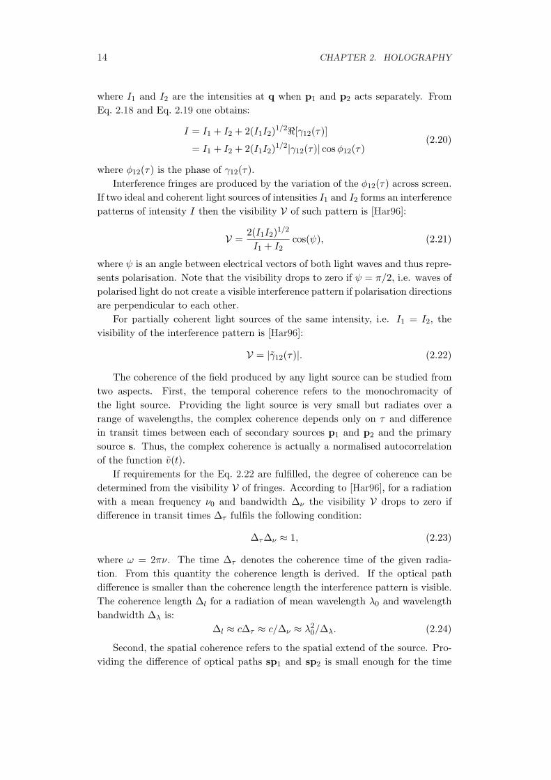
The nature of the diffraction can be illustrated on the well known Huygensprinciple proposed by C. Huygens. This principle states [Goo05] that the wave-front of a disturbance in a time t+∆t is an envelope of wavefronts of a secondarysources emanating from each point of the wavefront in a time t, see Fig. 2.4 forreference. This principle was modified by A. Fresnel who stated [Goo05] that thesecondary sources interfere with each other and the amplitude at each point ofthe wavefront is obtained as superposition of the amplitudes of all the secondarywavelets. This Huygens-Fresnel principle matches many optical phenomena and itwas also shown by G. Kirchhoff how this principle can be deduced from Maxwell’sequations.
Although this principle works in many cases its validity is in question [Goo05].
2.1. HOLOGRAPHY PHYSICS 17
t
t
t−∆t
t−∆tt+∆t
t+∆t
Direction of
propagation
Direction of
propagation
Figure 2.4: Huygens principle demonstrated on spherical (left) and planar (right)waves.
For example, it does not determine the direction of the wavefront propagation.It is only an intuitive choice that the wavefront diverges from the source and notconverges back to the source depending on the chosen orientation of the envelopeof the secondary wavelets. In this work, as in many others, this principle isaccepted as an appropriate description of the wave behavior of the light and itsinadequacies are neglected. Some of the synthesis methods are based on thisprinciple.
The intuitive way of the diffraction understanding is covered by the Huygensprinciple but more formal descriptions also exist. Some of them are presented inthe following material.
The mathematical description of the diffraction is quite difficult. It’s due tothe vectorial nature of the problem and many propagation medium propertieslike linearity, isotropy, homogeneity or dispersiveness that increase dimension ofthe problem. The basic diffraction model assumes an ideal material that is linear,isotropic, homogeneous, nondispersive and nonmagnetic. Under these conditions,the electromagnetic wave behavior can be described using only one scalar equationthat governs the behavior of both magnetic and electric field.
There is one other condition that further simplifies the diffraction model:considered diffraction structures are assumed to be large compared to the wave-length of the diffracted wave. All those simplifications and constraints turn thediffraction model into an approximation but even though the simplifications aresignificant ones they cause only small loss of accuracy and thus they are morethen appropriate in many situations.
There are two fundamental descriptions of the diffraction: the Kirchhoff for-mulation and the Rayleigh-Sommerfeld formulation [Goo05, LBL02]. Both for-mulations describe the light field in front of a screen or an aperture properly andaccurately. Nevertheless, the Kirchhoff formulation has a certain limitation as itfails to provide correct result if the examined point is closer to the screen than

18 CHAPTER 2. HOLOGRAPHY
the distance of several wavelengths. Also, it assumes that the field just behindthe aperture is zero and this is in contradiction with the physical experiments.Despite its limitations, the Kirchhoff formulation is widely used in practice.
The Kirchhoff formulation of diffraction is based on the integral theorem ofHelmholtz and Kirchhoff. The Helmholtz and Kirchhoff theorem states that thefield at any point can be expressed in terms of wave values on any closed surfacesurrounding that point [Goo05]. The theorem is an application of the Green’stheorem and the Helmholtz equation Eq. 2.11.
While the Helmholtz equation describes behavior of waves, the Green’s theo-rem defines a relation between two complex functions u(p) and g(p) of positionp. Let S be a closed surface surrounding a volume V . If u, v and their first andsecond partial derivatives in the inward normal direction are single-valued andcontinuous within and on S then:
−∫∫
S
∂u
∂ng − u
∂g
∂nds =
∫∫∫
Vg∇2u− u∇2g dv. (2.28)
The functions u(p) and g(p) provide twice continuously differentiable scalar fieldsmappings between V and S. If both functions satisfy the Helmholtz equationEq. 2.11 then [LBL02]:
−∫∫
S
∂u
∂ng − u
∂g
∂nds = 0 (2.29)
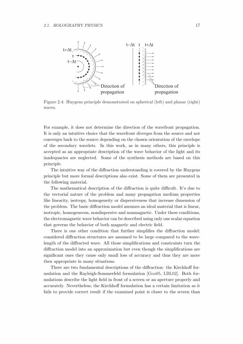
The goal of the diffraction formulation is do find a field at a point p0, seeFig. 2.5. For such purpose Kirchhoff formulation uses a boundary surface on oneside of the aperture. This boundary surface consists of two parts: a plane Sp closeto the aperture including its transparent portion Σ and a spherical surface Sε.Next, a couple of boundary condition known as Kirchhoff boundary conditionsare introduced in order to simplify the result. The boundary conditions describebehavior of field u in close neighbourhood to the screen.
The first condition is that the distribution of the field u across the surface Σincluding its derivate along normal n is no different from the same configurationwithout the screen. The second condition is that a portion of the surface close tothe screen Sp − Σ lies in a geometrical shadow an thus the function u as well asits derivate along the normal is zero. Both assumption are not physically validas they are never fulfilled completely but they simplify the equation by replacingone part of the enclosing surface just with the surface Σ. Refer to [Goo05] formore details.
The influence of the spherical surface vanishes as the radius of the sphericalsurface increases towards infinity [BW05]. By applying the boundary conditionsthe expression Eq. 2.29 is simplified to:
u(p0) =14π
∫∫
Σ
(∂u
∂ng − u
∂g
∂n
)ds, (2.30)
2.1. HOLOGRAPHY PHYSICS 19
p1
p2p0
Σ
Sp
Sε
R
r01r21
n
Figure 2.5: Kirchhoff formulation of diffraction by a plane screen. [Goo05]
where Σ is a transparent portion of the screen/aperture, u is a complex functiondescribing the wave distribution and g is a complex function, see below.
A further simplification of Eq. 2.30 is based on exploiting a proper Green’sfunction instead of the function g in the expression Eq. 2.29. One such functionthat satisfies the Helmholtz equation is:
g(p1) =exp(ikr01)
r01,
where r01 = p0 − p1 and r01 = |r01|. The derivation along normal can beapproximated according to an assumption on distances between observation pointp0 in enclosed volume and point p1 on the surface Σ. If r01 À λ then:
∂g
∂n=
exp(ikr01)r01
(ik − 1
r01
)cos(n, r01)
≈ ikexp(ikr01)
r01cos(n, r01).
Also, it is assumed that the screen or the aperture is illuminated by a sphericalwave emerging from the point p2. Hence, the field u at the point p1 is:
u(p1) =a exp(ikr21)
r21,
where r21 is distance between p1 and p2.Application of assumptions and substitutions described above leads to a form
known as the Fresnel-Kirchhoff diffraction formula:
u(p0) =a
iλ
∫∫
Σ
exp[ik(r21 + r01)]r21r01
[cos(n, r01)− cos(n, r21)
2
]ds, (2.31)

20 CHAPTER 2. HOLOGRAPHY
where a is a complex amplitude of the spherical wave, n is a normal of transparentportion Σ of the planar screen, and cos(a,b) is a cosine of angle between vectorsa and b. The vectors r01 and r21 are vectors of lengths r01 and r21 between anobservation point p0, point p1 on surface Σ, and source of the spherical wave p2.
More common formulation of the Fresnel-Kirchhoff formula can be obtainedby reorganising and substituting to Eq. 2.31 accordingly:
u(p0) =a
iλ
∫∫
Σu′(p1)
exp(ikr01)r01
ds. (2.32)
The interpretation of this equation is that the field at the point p0 is a super-position of infinite number of point sources on the surface Σ with a given complexamplitude u′. This is a consequence of the wave nature of light and this interpre-tation plays an important role in numerical reconstruction of the hologram, seebelow. Refer to [Goo05] for more details on the Kirchhoff formulation.
The Sommerfeld-Rayleigh formulation is a further enhancement of the Kirch-hoff formulation that removes inconsistent boundary conditions mentioned ear-lier. It removes the boundary condition from the function u by assuming thateither g or ∂g/∂n in Eq. 2.30 vanishes on a portion of the boundary surface closeto the aperture according to a proper definition of alternate Green’s function, seebelow. Alike the Kirchhoff solution, it assumes that the screen is planar.
In order to fulfil this assumption the formulation uses a second point p0′ that
is mirror image of the point p0. At this mirrored location a point source of thesame wavelength as the original one is positioned. Both wave sources oscillatewith π phase difference. For the π phase difference, a formula that describes thefield commonly known as the first Rayleigh-Sommerfeld solution is:
u(p0) =−14π
∫∫
Σu
∂g−∂n
ds, (2.33)
where g− = [exp(ijkr01)/r01] − [exp(ijkr′01)/r′01], i.e. it is a field constructed asa difference of fields generated by source at p0 and its mirror at p0
′. Note thatfunction g− vanishes on the transparent portion of planar screen, i.e. surface Σ.If |p0−p′0| À λ is assumed then it is possible to approximate normal derivate ofthe function g by:
∂g
∂n=
exp(ik|p0 − p′0|)|p0 − p′0|
(ik − 1
|p0 − p′0|)
α(n,p0 − p′0)
≈ ikexp(ik|p0 − p′0|)
|p0 − p′0|α(n,p0 − p′0),
where α(a,b) = (a · b)/(|a||b|) is a cosine of angle between vectors a and b. Byapplying this approximation to the alternate Green’s function g− and by the factthat g− vanishes on the transparent portion Σ of planar screen it is possible toobtain two formulae known as the Rayleigh-Sommerfeld diffraction formula. For
2.1. HOLOGRAPHY PHYSICS 21
more details on derivation of these formulae refer to [Goo05, LBL02, Mie02]. Thefirst configuration that has a π phase difference in phases is:
uI(p0) =a
iλ
∫∫
Σ
exp[ik(r21 + r01)]r21r01
cos(n, r01) ds. (2.34)
The second configuration that has zero phase difference in phases is:
uII(p0) = − a
iλ
∫∫
Σ
exp[ik(r21 + r01)]r21r01
cos(n, r21) ds. (2.35)
Note that both first and the second Rayleigh-Sommerfeld formulation resem-bles the Kirchhoff-Fresnel diffraction formula with the difference in sign and thelast cosine-based component. It can also be shown that the Kirchhoff solutionis an average of both first and the second Rayleigh-Sommerfeld solution. Kirch-hoff and Rayleigh-Sommerfeld solutions are almost identical for small angles andlarger distance but they differ at distances closer to the aperture. For more detailon comparison and discussion on consequences beyond scope of this work referto [Goo05].
2.1.6 Wave propagation
The propagation of the wave in a free space plays an important role in the holo-gram reconstruction and synthesis. Propagation determines the final configu-ration of a light field at a hologram frame due to a given scene radiation. Theconsequent propagation in a reversed direction can reconstruct the recorded sceneform a hologram. The propagation is driven by the diffraction formulae describedin the Sec. 2.1.5.
The propagation of a wave is carried out by a change of phase. At this pointis important to specify whetter the propagation is done by adding or subtractinga value from the phase. Since the time dependent component exp(−iωt) of thewavefunction Eq. 2.9 rotates in a clockwise direction the waves emitted earlier intime have phase greater than waves emitted later. The later the wave is emittedthe closer it is to its source. Thus, if waves are to be propagated from the sourcethen the phase has to be increased.
In order to minimise the confusion from signs of phases, it is assumed thatthe propagation of the wave is examined in a direction of a positive Z-axis. Thisalso simplifies equation for propagation in a direction parallel to the Z-axis. Ifother configurations are required then it is always possible to transform them sothat eventually the propagation is done in a direction parallel to the Z-axis.
Huygens-Fresnel principle
The Huygens-Fresnel principle states that the wavefront of a disturbance in a timet+∆t is an envelope of wavefronts of secondary sources emanating from each point

22 CHAPTER 2. HOLOGRAPHY
of the wavefront in a time t. The secondary sources interfere with each other andthe amplitude at each point of the wavefront is obtained as superposition of theamplitudes of all the secondary wavelets [Goo05]. This Huygens-Fresnel principleis supported by both Kirchhoff and Rayleigh-Sommerfeld diffraction formulae.Using the first Rayleigh-Sommerfeld solution from Eq. 2.34, the Huygens-Fresnelprinciple is [LBL02]:
uI(p0) =1iλ
∫∫
Σu(p1)
exp(ikr01)r01
cos θ ds, (2.36)
where u(p1) represents a secondary point source positioned at the point p1 withinthe aperture Σ. The complex amplitudes of the secondary sources are propor-tional to the amplitude at the point p1 of the original wave and the phases areπ/2 before the phase of the original wave due to the factor 1/i. Note that dueto the Rayleigh-Sommerfeld solution, the aperture Σ is expected to be a planeor its portion and thus all following solutions for the wave propagation solve theproblem of propagating between two parallel planes, if not noted otherwise.
The important aspect of Eq. 2.36 is that it is basically a convolution integraland it can be expressed as:
u(p0) =∫∫
Σh(p0,p1)u(p1) ds, (2.37)
where h(p0,p1) is the impulse response function that is given explicitly by:
h(p0,p1) =1iλ
exp(ikr01)r01
cos θ.
Fresnel and Fraunhofer approximation
As noted in the previous section, it is possible to express the Huygens-Fresnelprinciple in terms of the first Rayleigh-Sommerfeld solution. The angle θ issubtended by the outward normal n and the vector r01. The cosine of this anglecan be also expressed as following:
cos θ =z
r01,
and assuming the situation depicted in the Fig. 2.6 it is possible to express theHuygens-Fresnel principle Eq. 2.36 as following:
u(x, y) =z
iλ
∫∫
Σu(ξ, η)
exp(ikr01)r201
dξ dη, (2.38)
where r01 = [z2 + (x − ξ)2 + (y − η)2]1/2. All following approximations simplifythe expression for r01 because it contains square root function that does not allowexploiting the Fourier transform that greatly reduces the computation complexityof the expression.
2.1. HOLOGRAPHY PHYSICS 23
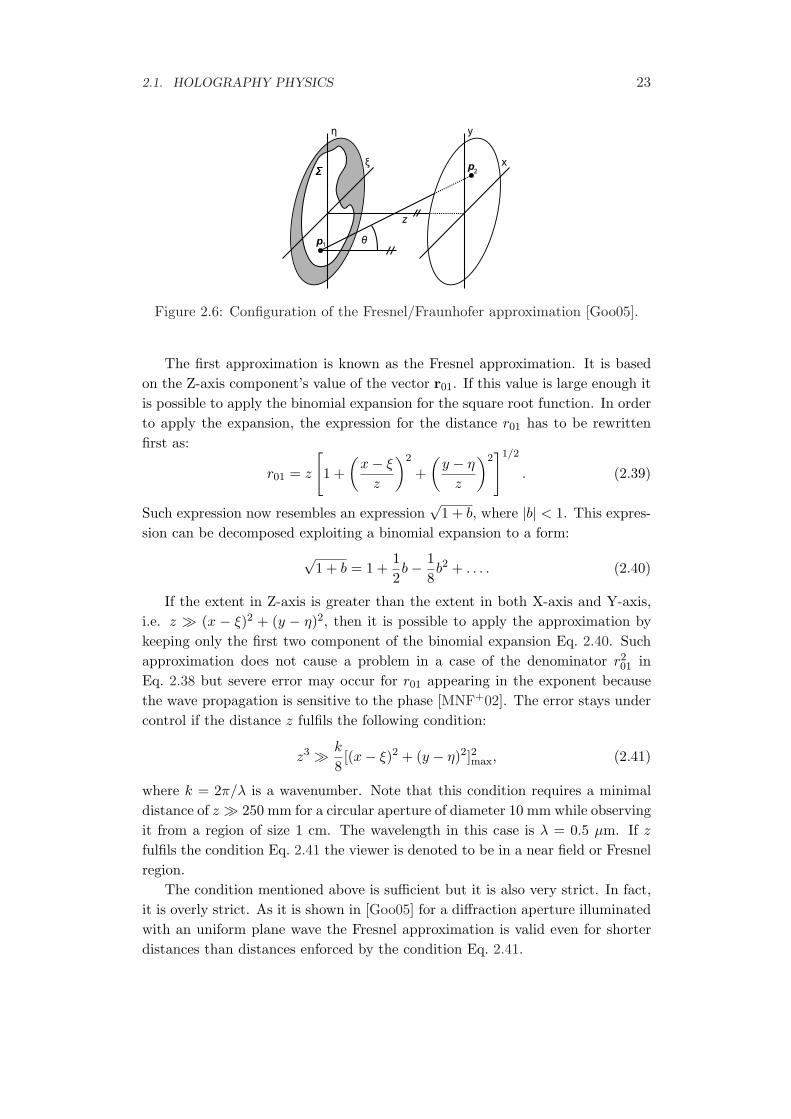
Figure 2.6: Configuration of the Fresnel/Fraunhofer approximation [Goo05].
The first approximation is known as the Fresnel approximation. It is basedon the Z-axis component’s value of the vector r01. If this value is large enough itis possible to apply the binomial expansion for the square root function. In orderto apply the expansion, the expression for the distance r01 has to be rewrittenfirst as:
r01 = z
[1 +
(x− ξ
z
)2
+(
y − η
z
)2]1/2
. (2.39)
Such expression now resembles an expression√
1 + b, where |b| < 1. This expres-sion can be decomposed exploiting a binomial expansion to a form:
√1 + b = 1 +
12b− 1
8b2 + . . . . (2.40)
If the extent in Z-axis is greater than the extent in both X-axis and Y-axis,i.e. z À (x − ξ)2 + (y − η)2, then it is possible to apply the approximation bykeeping only the first two component of the binomial expansion Eq. 2.40. Suchapproximation does not cause a problem in a case of the denominator r2
01 inEq. 2.38 but severe error may occur for r01 appearing in the exponent becausethe wave propagation is sensitive to the phase [MNF+02]. The error stays undercontrol if the distance z fulfils the following condition:
z3 À k
8[(x− ξ)2 + (y − η)2]2max, (2.41)
where k = 2π/λ is a wavenumber. Note that this condition requires a minimaldistance of z À 250 mm for a circular aperture of diameter 10 mm while observingit from a region of size 1 cm. The wavelength in this case is λ = 0.5 µm. If z
fulfils the condition Eq. 2.41 the viewer is denoted to be in a near field or Fresnelregion.
The condition mentioned above is sufficient but it is also very strict. In fact,it is overly strict. As it is shown in [Goo05] for a diffraction aperture illuminatedwith an uniform plane wave the Fresnel approximation is valid even for shorterdistances than distances enforced by the condition Eq. 2.41.
24 CHAPTER 2. HOLOGRAPHY
Nevertheless, by fulfilling the condition it is possible to substitute the Eq. 2.39to the first two components of the binomial expansion Eq. 2.40 thus obtaining:
r01 ≈ z +(x− ξ)2 + (y − η)2
2z.. (2.42)
Putting Eq. 2.42 and Eq. 2.38 together one obtains this resulting expressionknown as the Fresnel diffraction integral:
uz(x, y) =exp(ikz)
iλz
∫∫ ∞
−∞u0(ξ, η) exp
[ik
(x− ξ)2 + (y − η)2
2z
]dξ dη, (2.43)
where u0(ξ, η) is a diffraction pattern at the aperture. This expression can berewritten into a form that resembles the Fourier transform. The fast Fouriertransform – FFT can be exploited for evaluating thus reducing the computationalcomplexity significantly:
uz(x, y) =exp(ikz)
iλzexp
(ik
x2 + y2
2z
)
×∫∫ ∞
−∞
{u0(ξ, η) exp
(ik
ξ2 + η2
2z
)}exp
(−ik
xξ + yη
z
)dξ dη.
(2.44)
If the distance z is increased even more it is possible to apply another ap-proximation that consist in neglecting another components of the integral. Suchapproximation is known as the Fraunhofer approximation and it is applicableonly if:
z À k(ξ2 + η2)max
2. (2.45)
This condition has even higher demands on the distance z than the conditionEq. 2.41 has. For a circular aperture with a diameter of 10mm and for a wave withwavelength 0.5µm the distance z has to be z À 300m. If z fulfils the conditionEq. 2.45 the viewer at that distance is denoted to be in far field or Fraunhoferregion. By satisfying the condition of the Fraunhofer region the Eq. 2.44 isreduced to the following:
uz(x, y) =exp(ikz)
iλzexp
(ik
x2 + y2
2z
)
×∫∫ ∞
−∞u0(ξ, η) exp
(−j2π
xξ + yη
λz
)dξ dη. (2.46)
The integral in the Eq. 2.46 resembles a Fourier transformation of the aperturedistribution u0. If a normalised intensity is the final product of a propagationthen the Fraunhofer approximation constitutes only Fourier transform of u0. Themultiplicative phase factors are not applied as they have no influence on theintensity, see Eq. 2.12. The Fourier transform is evaluated at frequencies:
fX = x/λz,
fY = y/λz.

2.1. HOLOGRAPHY PHYSICS 25
So far, the Fresnel approximation assumed a propagation of diffraction patternbetween two planes along the Z-axis where both planes are parallel and theirorigins lie on the Z-axis. Yet, it is possible to enhance the Fresnel approximationformula so it is capable of handling tilted planes such as that depicted in theFig. 2.7 as well [YAC02].
Figure 2.7: Tilted plane configuration for application of Fresnel approxima-tion [YAC02].
The approach is based on simplifying the expression for the distance. Ifthe target diffraction pattern uz,θ(x, y) is examined on a plane that is tilted asdepicted in the Fig. 2.7 then the expression for the distance required for theRayleigh-Sommerfeld integral is:
r =[(y0 sin θ − z)2 + (x0 − x)2 + (y0 cos θ − y)2
]1/2. (2.47)
By introducing the r′ = (x2+y2+z2)1/2 to the Eq. 2.47 the binomial expansioncan be applied. After the expansion, it is possible to neglect all terms but the firsttwo as it is done in a case of the Fresnel approximation. The resulting expressionis substituted to this modified Rayleigh-Sommerfeld integral:
uz,θ(x, y) = − a
iλ
∫∫
Σu0(x0, y0)
exp(ikr)r
χ(x0, y0, x, y) dx0 dy0,
where u0(x0, y0) is a source of the diffraction pattern and χ(x0, y0, x, y) is aninclination factor that is close to 1 if condition for the Fresnel approximation isfulfilled. By reorganising and further substitution the Eq. 2.48 is obtained thatresembles the Fourier transform:
uz,θ(ξ, η) = exp(ikr′)∫∫
Σu0(x0, y0) exp
(ik
x20 + y2
0
2z
)
exp [−i2π(ξx0 + ηy0)] dx0 dy0,
(2.48)
where ξ = x/(λr′) and η = (y cos θ + z sin θ)/(λr′). Note that the result isrespective to a plane deformed by coordinates ξ and η and result is valid only ifthe condition for the Fresnel approximation is fulfilled.
26 CHAPTER 2. HOLOGRAPHY
Diffraction condition and diffraction orders
A term diffraction condition regards to a planar wave diffracted on a thin cosinegrating [Goo05, Kra04]. The cosine grating is a thin planar cosine amplitudegrating with a amplitude transmittance function:
tA(ξ, η) = exp[12
+m
2cos
(2π
ξ
Λξ
)]rect
(ξ
2w
)rect
( η
2w
), (2.49)
where ξ and η are coordinates on a grating, 2w is the width/height of the rect-angular aperture, m represents a difference between maximum and minimum ofthe tA, and Λξ is the grating’s period.
If such grating is illuminated by a unit amplitude planar wave then diffrac-tion occurs. By applying the convolution theorem to tA it is possible to obtainthe Fourier transform of tA that can be utilised to get the grating’s Fraunhoferdiffraction pattern, i.e. a diffraction pattern in the far field:
u(x, y) =a
i2λzexp
[ikz + i
k
2z(x2 + y2)
]sinc
(2wy
λz
)
×{
sinc(
2wx
λz
)+
m
2sinc
[2w
λz
(x +
λz
Λξ
)]+
m
2sinc
[2w
λz
(x− λz
Λξ
)]}
(2.50)
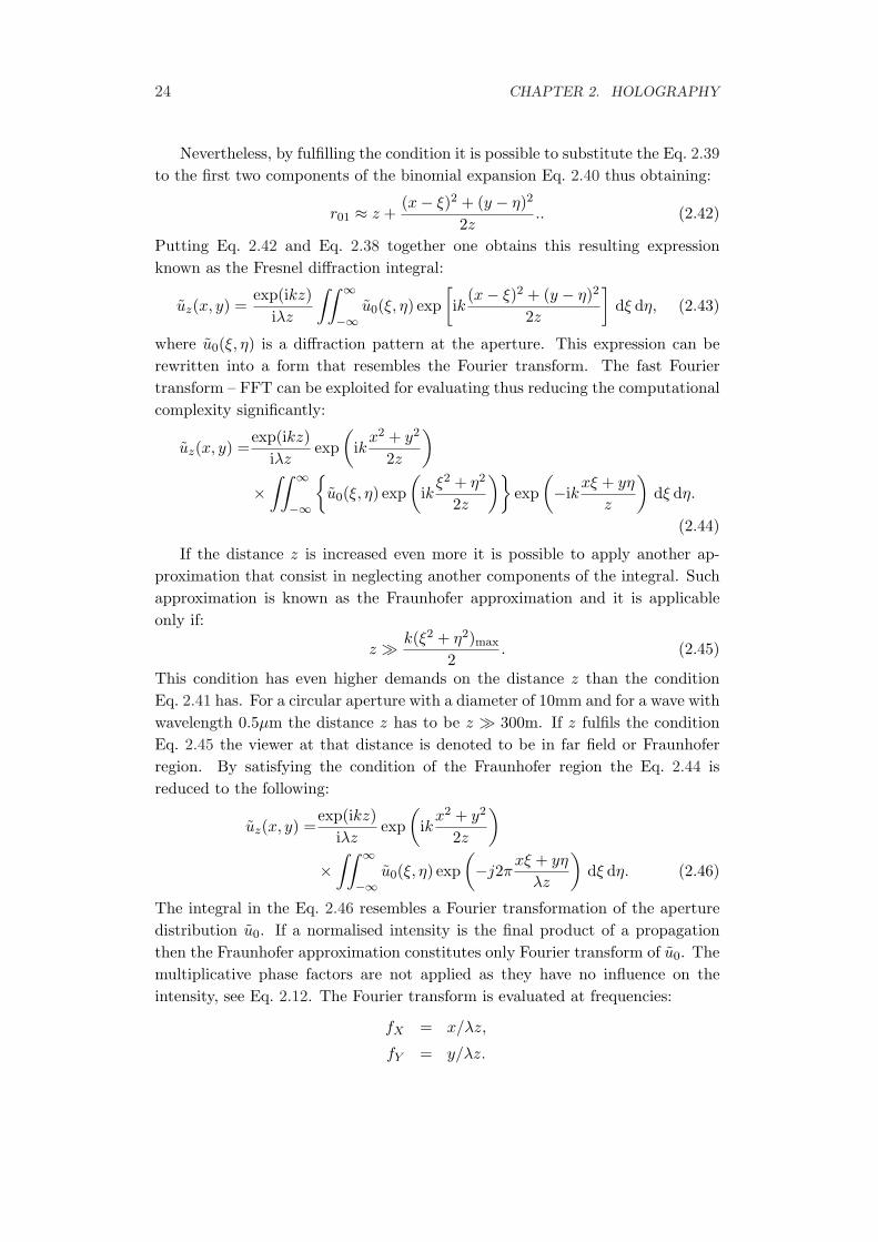
The intensity of the diffraction pattern u is its magnitude squared. Thismeans that the intensity of the Eq. 2.50 is a sum of squared sinc functions. Theintensity is depicted in the Fig. 2.8.
Figure 2.8: Intensity of a Fraunhofer diffraction pattern due to a thin amplitudecosine grating [Goo05].
Peaks in the Fig. 2.8 constitute so called diffraction orders and they representenergy deflected by the aperture. The largest central peak is called the zero orderand represents the undiffracted wave, i.e. a wave having the same direction asthe incident one. Zero order also contains the greatest amount of energy of theoriginal incident planar wave. The two second largest peaks on sides are called

2.1. HOLOGRAPHY PHYSICS 27
the first orders and represent planar waves diffracted according to the diffractioncondition, see below.
The incident energy is divided into individual diffraction orders. The fractionfor each order is determined as the squared coefficient of the delta function thatappear in the Fourier transform of the expression Eq. 2.49. Note that while thesinc functions in the Fourier transform of Eq. 2.49 spreads the energy, the deltafunction determine the power in each order. The zero order obtains 1/4 = 25.0%of the incident wave power, the maximum portion for the first order is 1/16 =6.25% of the incident power; the rest is absorbed by the grating or reflected. Thepercentage of the energy diffracted as the first order is known as the diffractionefficiency of the grating.
A better diffraction efficiency of up to 33.8% has the thin sinusoidal phasegrating that employs complex amplitude transmittance instead of the real onein the Eq. 2.49. This kind of grating also produces higher orders then the firsts.The approach for deriving the respective diffraction order’s energy is similar tothe amplitude grating so it will not be included here. Refer to [Goo05] for moredetails.
Basically, each diffraction order is the original incident planar wave that ispropagated to a different direction and is carrying different amount of energy.The direction of the propagation for a given diffraction order is determined fromthe optical path difference of individual ”rays” [Goo05]. The difference for agiven order has to be an integer multiple of λ because only in such case a planarwavefront is formed. Thus, for a transmission grating, the incoming plane waveis diffracted according to:
sin θξ2 = sin θξ1 + qλ
Λ, (2.51)
where θξ1 is an angle of the incident wave, θξ2 is an angle of the diffracted wavefor given order q, and Λ is the period of the grating, see Fig. 2.9.
Figure 2.9: Diffraction grating and diffraction condition.

28 CHAPTER 2. HOLOGRAPHY
Propagation in Angular Spectrum
The Fresnel approximation allows computing a propagation of a diffraction pat-tern but it has restrictions on distance according to the condition Eq. 2.41. Eventhough this condition is unnecessarily strict and it is possible to apply the Fresnelapproximation even for shorter distances, still, it is not applicable for a regioncloser to a diffracting plane with known diffraction pattern distribution u0 unlessthe third or higher components of the binomial expansion are taken into account.
For shorter distances the Rayleigh-Sommerfeld diffraction integral, see Eq. 2.34,has to be employed. Unfortunately, an implementation of this integral has an un-pleasantly high computation complexity and thus rendering this approach almostuseless. However, a slightly different approach can be formulated using a Fouriertransform of the diffraction pattern. The frequencies obtained from the Fouriertransform are called the angular spectrum [EO06, Goo05, TB93].
If an angular spectrum F (kx, ky) of a diffraction pattern is known then it ispossible to determine a field u at a given point p as:
u(p) =∫∫
F (kx, ky) exp(−ik · p) dkx dky, (2.52)
where kz = (k2−k2x−k2
y)1/2. It is assumed that k2
z ≥ 0. If in any case k2z becomes
negative then kz becomes a complex number. A wave with kz ∈ C is known asan evanescent wave [BW05]. Such wave is propagated as well but its amplitudedecays exponentially with increasing |z|. The exponential nature of attenuationis apparent from substitution of complex-valued kz to the Eq. 2.52.
For a plane % : z = 0, the field is determined according to the following:
u0(x, y) =∫∫
F (kx, ky) exp[−i(kxx + kyy)] dkx dky. (2.53)
From Eq. 2.53 is apparent that the angular spectrum F is proportional to theFourier transform of the diffraction pattern u0 on the plane %. More precisely,that F = F {u0} /(2π)2.
From a knowledge of some diffraction pattern’s angular spectrum it is possibleto predict the diffraction pattern at an arbitrary distance along the Z-axis. Wavesare propagated according to the Eq. 2.52. If the phase shift term exp(−ik · p) isexpanded properly then it is possible to obtain an expression that resembles theFourier transform as well. Note that individual wavevector components contains2π/λ since the length of a wavevector is the wavenumber.:
u(p) =∫∫ {
F (kx, ky) exp(−ikzz)}
exp[−i(kxx + kyy)] dkx dky. (2.54)
According to the Eq. 2.54 the diffraction pattern u on a plane that is parallel tothe source plane and is located at the distance z along positive Z-axis is computed
2.1. HOLOGRAPHY PHYSICS 29
by employing this expression:
u = F−1 {F {u0} exp(−ikzz)} , (2.55)
where u is a diffraction pattern on a target plane while u0 is diffraction patternon a source plane.
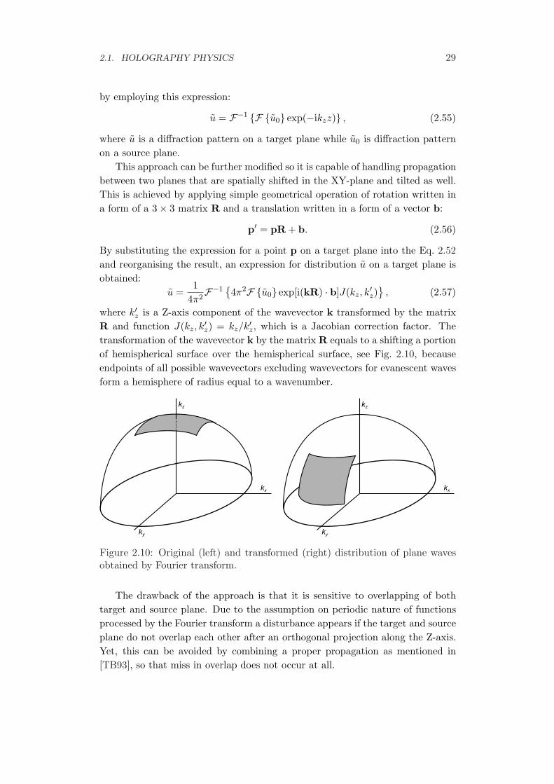
This approach can be further modified so it is capable of handling propagationbetween two planes that are spatially shifted in the XY-plane and tilted as well.This is achieved by applying simple geometrical operation of rotation written ina form of a 3× 3 matrix R and a translation written in a form of a vector b:
p′ = pR + b. (2.56)
By substituting the expression for a point p on a target plane into the Eq. 2.52and reorganising the result, an expression for distribution u on a target plane isobtained:
u =1
4π2F−1
{4π2F {u0} exp[i(kR) · b]J(kz, k
′z)
}, (2.57)
where k′z is a Z-axis component of the wavevector k transformed by the matrixR and function J(kz, k
′z) = kz/k′z, which is a Jacobian correction factor. The
transformation of the wavevector k by the matrix R equals to a shifting a portionof hemispherical surface over the hemispherical surface, see Fig. 2.10, becauseendpoints of all possible wavevectors excluding wavevectors for evanescent wavesform a hemisphere of radius equal to a wavenumber.
Figure 2.10: Original (left) and transformed (right) distribution of plane wavesobtained by Fourier transform.
The drawback of the approach is that it is sensitive to overlapping of bothtarget and source plane. Due to the assumption on periodic nature of functionsprocessed by the Fourier transform a disturbance appears if the target and sourceplane do not overlap each other after an orthogonal projection along the Z-axis.Yet, this can be avoided by combining a proper propagation as mentioned in[TB93], so that miss in overlap does not occur at all.
30 CHAPTER 2. HOLOGRAPHY
2.2 Optical holography
The holography in general is quite wide scientific area. It can be divided intoseveral groups. Each group have a different goal according to the primary appli-cation. For this work the relevant branch of holography is the one dealing withrealistic image recording and reproduction. This branch can be further dividedinto two sub branches – optical holography and digital holography.
The optical holography is a real thing that needs actual lasers and photo-graphic materials for recording and reproducing holographic images. Opticalholography stands on the physical phenomenon of diffraction described in theSec. 2.1.5. On the other hand, the digital holography is a numerical alternationof the optical holography. It replaces the real diffraction with a numerical simu-lation of the diffraction to obtain holograms. It also replaces static photographicmaterial with computer driven electronic spatial light modulators for reproducingthe holographic images.
This section describes the principle of the optical holography. Digital holog-raphy is described later on in the Sec. 2.3.
2.2.1 Holography principle
Holography is about recording and reproducing a light field. A light field is ateach point determined by an amplitude and phase. In a case of classical photog-raphy the light field is focused onto a photographic material and incident energyis integrated over some time. The photographic material reacts accordingly andexposed places become dark. This process therefore records the intensity infor-mation but omits the direction information. That is the reason, why reproducedimage looks flat, without depth.
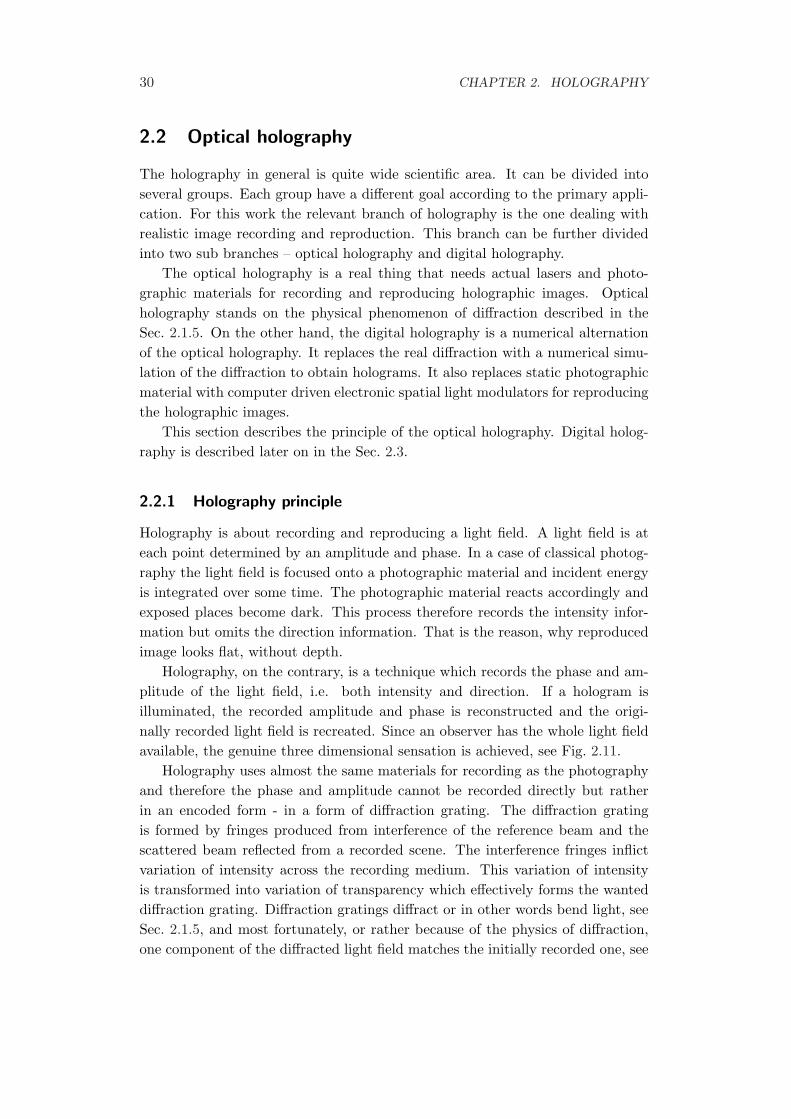
Holography, on the contrary, is a technique which records the phase and am-plitude of the light field, i.e. both intensity and direction. If a hologram isilluminated, the recorded amplitude and phase is reconstructed and the origi-nally recorded light field is recreated. Since an observer has the whole light fieldavailable, the genuine three dimensional sensation is achieved, see Fig. 2.11.
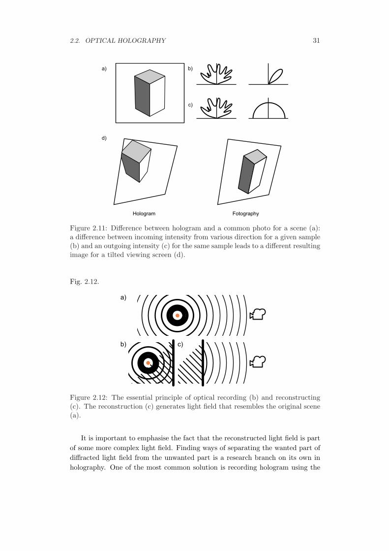
Holography uses almost the same materials for recording as the photographyand therefore the phase and amplitude cannot be recorded directly but ratherin an encoded form - in a form of diffraction grating. The diffraction gratingis formed by fringes produced from interference of the reference beam and thescattered beam reflected from a recorded scene. The interference fringes inflictvariation of intensity across the recording medium. This variation of intensityis transformed into variation of transparency which effectively forms the wanteddiffraction grating. Diffraction gratings diffract or in other words bend light, seeSec. 2.1.5, and most fortunately, or rather because of the physics of diffraction,one component of the diffracted light field matches the initially recorded one, see
2.2. OPTICAL HOLOGRAPHY 31
b)
c)
Hologram Fotography
a)
d)
Figure 2.11: Difference between hologram and a common photo for a scene (a):a difference between incoming intensity from various direction for a given sample(b) and an outgoing intensity (c) for the same sample leads to a different resultingimage for a tilted viewing screen (d).
Fig. 2.12.
a)
b) c)
Figure 2.12: The essential principle of optical recording (b) and reconstructing(c). The reconstruction (c) generates light field that resembles the original scene(a).
It is important to emphasise the fact that the reconstructed light field is partof some more complex light field. Finding ways of separating the wanted part ofdiffracted light field from the unwanted part is a research branch on its own inholography. One of the most common solution is recording hologram using the
32 CHAPTER 2. HOLOGRAPHY
off-axis configuration, see Sec. 2.2.3 for more details.The following material contains description of different hologram recording
principles. Advantages and disadvantages of each of them are discussed.
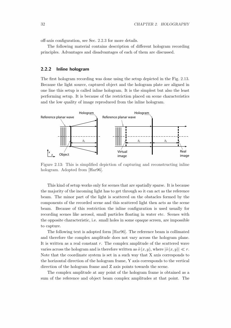
2.2.2 Inline hologram
The first hologram recording was done using the setup depicted in the Fig. 2.13.Because the light source, captured object and the hologram plate are aligned inone line this setup is called inline hologram. It is the simplest but also the leastperforming setup. It is because of the restriction placed on scene characteristicsand the low quality of image reproduced from the inline hologram.
Hologram Hologram
Reference planar wave Reference planar wave
ObjectVirtual
image
Real
image
Figure 2.13: This is simplified depiction of capturing and reconstructing inlinehologram. Adopted from [Har96].
This kind of setup works only for scenes that are spatially sparse. It is becausethe majority of the incoming light has to get through so it can act as the referencebeam. The minor part of the light is scattered on the obstacles formed by thecomponents of the recorded scene and this scattered light then acts as the scenebeam. Because of this restriction the inline configuration is used usually forrecording scenes like aerosol, small particles floating in water etc. Scenes withthe opposite characteristic, i.e. small holes in some opaque screen, are impossibleto capture.
The following text is adopted form [Har96]. The reference beam is collimatedand therefore the complex amplitude does not vary across the hologram plane.It is written as a real constant r. The complex amplitude of the scattered wavevaries across the hologram and is therefore written as o (x, y), where |o (x, y)| ¿ r.Note that the coordinate system is set in a such way that X axis corresponds tothe horizontal direction of the hologram frame, Y axis corresponds to the verticaldirection of the hologram frame and Z axis points towards the scene.
The complex amplitude at any point of the hologram frame is obtained as asum of the reference and object beam complex amplitudes at that point. The
2.2. OPTICAL HOLOGRAPHY 33
resultant optical intensity is then obtained using Eq. 2.14 as
I (x, y) = |r + o (x, y)|2 ,
= r2 + |o (x, y)|2 + ro (x, y) + ro∗ (x, y) ,(2.58)
where o∗ (x, y) is the complex conjugate of o (x, y).The optical intensity is recorded on a transparency. If it is assumed that
amplitude transmittance is a linear function of the intensity then it can be writtenas
t = t0 + βTI, (2.59)
where t0 is a constant background transmittance, T is the exposure time, and β isa parameter determined by the photographic material. When 2.58 is substitutedinto 2.59 the amplitude of this transparency is
t (x, y) = t0 + βT[r2 + |o (x, y)|2 + ro (x, y) + ro∗ (x, y)
]. (2.60)
To reconstruct the recorded scene, the hologram is placed on the same positionas during recording and illuminated by the very same reference beam and thetransmitted complex amplitude by the hologram can be then written as
u (x, y) = rt
= r(t0 + βTr2
)+ βTr |o (x, y)|2
+ βTr2o (x, y) + βTr2o∗ (x, y) .
(2.61)
The expression Eq. 2.61 consists of four terms. The frist term r(t0 + βTr2
)
constitutes the directly transmitted beam. The second term βTr |o (x, y)|2 is ex-tremely small in comparison with the others since it has been assumed initiallythat |o (x, y)| ¿ r and can be therefore neglected. The third term βTr2o (x, y)is, except for a constant factor, identical with the object beam. This light fieldconstitutes the reconstructed image. Since this image is located behind the trans-parency and the reconstructed light field appears to diverge from it, it is calledthe virtual image . The fourth term also represents the originally captured lightfield except it is complex conjugate of the field. This field converges to form socalled real image, which is inverted by the Z axis.
The low quality of images reproduced from inline holograms is caused by thefact that the reconstructed virtual image superposes with the directly transmittedreference beam and with the blurred real image. This fact was the reason forlow interest about holography at the beginning. The efficient way of separatingthe virtual image from its real counterpart and from the zero order beam wasdeveloped by Leith and Upatnieks in 60’ and it is introduced in the followingsection.
34 CHAPTER 2. HOLOGRAPHY
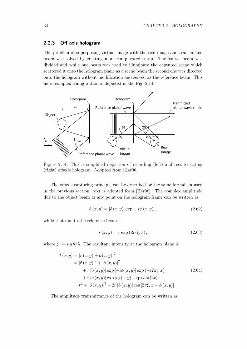
2.2.3 Off axis hologram
The problem of superposing virtual image with the real image and transmittedbeam was solved by creating more complicated setup. The source beam wasdivided and while one beam was used to illuminate the captured scene whichscattered it onto the hologram plane as a scene beam the second one was directedonto the hologram without modification and served as the reference beam. Thismore complex configuration is depicted in the Fig. 2.14.
Hologram
Object
Reference planar wave
Reference planar wave
Hologram
Virtual
image
Real
image
Tranmitted
planar wave + halo
Figure 2.14: This is simplified depiction of recording (left) and reconstructing(right) offaxis hologram. Adopted from [Har96].
The offaxis capturing principle can be described by the same formalism usedin the previous section, text is adopted form [Har96]. The complex amplitudedue to the object beam at any point on the hologram frame can be written as
o (x, y) = |o (x, y)| exp [−iφ (x, y)] , (2.62)
while that due to the reference beam is
r (x, y) = r exp (i2πξrx) , (2.63)
where ξr = sin θ/λ. The resultant intensity at the hologram plane is
I (x, y) = |r (x, y) + o (x, y)|2= |r (x, y)|2 + |o (x, y)|2
+ r |o (x, y)| exp [−iφ (x, y)] exp (−i2πξrx)
+ r |o (x, y)| exp [iφ (x, y)] exp (i2πξrx)
= r2 + |o (x, y)|2 + 2r |o (x, y)| cos [2πξrx + φ (x, y)].
(2.64)
The amplitude transmittance of the hologram can be written as

2.2. OPTICAL HOLOGRAPHY 35
t (x, y) = t0 + βT{|o (x, y)|2+ r |o (x, y)| exp [−iφ (x, y)] exp (−i2πξrx)
+ r |o (x, y)| exp [iφ (x, y)] exp (i2πξrx)}(2.65)
To reconstruct the image, the hologram is illuminated by the very same refer-ence beam used for recording. The complex amplitude u (x, y) of the transmittedwave can be written as:
u (x, y) = r (x, y) t (x, y) ,
= u1 (x, y) + u2 (x, y) + u3 (x, y) + u4 (x, y)(2.66)
where
u1 (x, y) = t0 exp (i2πξrx) (2.67)
u2 (x, y) = βTr |o (x, y)|2 exp (i2πξrx) (2.68)
u3 (x, y) = βTr2o (x, y) (2.69)
u4 (x, y) = βTr2o∗ (x, y) exp (i4πξrx) (2.70)
The first term u1 (x, y) constitutes the directly transmitted reference beamattenuated by the constant factor. The second term u2 (x, y) is responsible forsome sort of halo surrounding the reference beam. The angular spread of thehalo depends on the extend of the object. The third term u3 (x, y) is identicalwith the original object wave so it is the virtual image. And finally the fourthterm u4 (x, y) is the conjugate of the original object wave so it is the real image.However, in a case of the off axis hologram, there is additional term exp (i4πξrx)which indicates that the conjugate wave is deflected from the Z axis at an angleapproximately twice that which the reference wave makes with it.
For this reason, the real and virtual image are reconstructed at different anglesfrom the directly transmitted beam and from each other. If the offset angle θ islarge enough the three will not overlap. This method therefore eliminates all thedrawbacks of the Gabor’s inline hologram.
The minimum value of the offset angle θ required to ensure that each of theimages can be observed without any interference from its twin image, as well asfrom the directly transmitted beam and the halo of scattered light surroundingit, is determined by the minimum spatial carrier frequency ξr for which there isno overlap between the angular spectra of the third na fourth terms, and thoseof the first and second terms. According to the [Har96] they will not overlap ifthe offset angle θ is chosen so that the spatial carrier frequency ξr satisfies thecondition
ξr ≥ 3ξmax, (2.71)
36 CHAPTER 2. HOLOGRAPHY
where ξmax is the highest frequency in the spatial frequency spectrum of theobject beam.
The restriction on scene characteristic found in the inline hologram does notapply in a case of the offaxis hologram. More complex and interesting scenes canbe recorded and consequently reconstructed. However, the off axis configurationis more sensitive to the coherence length of the light source. The difference ofpath lengths of the reference and the scene beam must not exceed the coherencelength of the light source used.
2.2.4 Additional hologram types
Apart from the configurations described in Sec. 2.2.2 and Sec. 2.2.3, there are sev-eral other hologram recording configurations. In this section these configurationsare described:
• Fourier hologram
• Image hologram
• Fraunhofer hologram
Fourier hologram
Setup for capturing Fourier hologram is similar to the setup used for recordinginline hologram. Additionally, a lens is introduced between hologram plane andrecorded object. Lens is placed such that the hologram plane is in the back focalplane of the lens and the recorded object and reference light source is in the frontfocal plane of the lens.
The lens works in such way that the back focal plane contains Fourier trans-form of the light field in the front focal plane. The Fourier hologram is thereforeformed from interference of Fourier transforms of recorded object and referencebeam.
Utilising the same formalism used in the cases of inline and off axis holograms,the complex amplitude leaving the object plane is o (x, y), its complex amplitudeat the hologram plate located in the back focal plane of the lens is
O (ξ, η) = F {o (x, y)} . (2.72)
The reference beam is derived from the point source also located in the frontfocal plane of the lens. If δ (x + b, y) is the complex amplitude of the light fieldleaving this pint source, the complex amplitude of the reference light field at thehologram plane can be written as
R (ξ, η) = e−i2πξb. (2.73)

2.2. OPTICAL HOLOGRAPHY 37
The intensity of the interference pattern produced by those two waves istherefore
I (ξ, η) =1 +∣∣∣O (ξ, η)
∣∣∣2+ O (ξ, η) exp (i2πξb) +
O∗ (ξ, η) exp (−i2πξb) .(2.74)
To reconstruct the image, the processed hologram is placed in the front focalplane of the lens and illuminated with a collimated beam of monochromatic light.If it is assumed that this wave has unit amplitude and that the amplitude trans-mittance of the processed hologram is a linear function of I (ξ, η), the complexamplitude of the wave transmitted by the hologram is
U (ξ, η) = t0 + βTI (ξ, η) . (2.75)
The complex amplitude in the back focal plane of the lens is then the Fouriertransform of U (ξ, η),
u (x, y) = F {U (ξ, η)} ,
= (t0 + βT ) δ (x, y) + βT o (x, y) ? o (x, y)
+ βT o (x− b, y) + βT o∗ (−x + b,−y) .
(2.76)
The wave corresponding to the first term on the right-hand side of Eq. 2.76comes to a focus on the axis, while that corresponding to the second term formsa halo around it. The third term produces an image of the original object, shifteddownwards by a distance b, while the fourth term gives rise to a conjugate image,inverted and shifted upwards by the same distance b. Both images are real andcan be recorded on a photographic film placed in the back focal plane of the lens.Since the film records the intensity distribution in the image, the conjugate imagecan be identified only by the fact that it is inverted. More details can be foundin [Har96].
Image holograms
Image holograms are not recordings of object but recording of the real image ofthe object. The lens is used to project the real image of the object. With sucharrangement it is possible to position the hologram plate in such manner that theimage of the object straddles the plate. The reconstructed image is then formedin the same position with respect to the hologram, so that part of the imageappears to be in front of the hologram and the remainder is behind it.
Image can be reproduced from an image hologram using a source of apprecia-ble size and spectral bandwidth and will still produce an acceptably sharp image.They have also increased luminosity. However, the viewing angles are limited bythe aperture of the imaging lens. More details about image holograms can befound in [Har96].

38 CHAPTER 2. HOLOGRAPHY
Fraunhofer hologram
Fraunhofer holograms are special case of the inline holograms. This class ofholograms impose further constraint onto the scene configuration. In this case,the captured scene has to be small enough for its Fraunhofer diffraction pattern,see Sec. 2.1.6, to form on the photographic plate. The object is small enough ifits distance z0 and lateral dimensions x0 and y0 satisfies the far-field condition:
z0 À(x2
0 + y20
)/λ. (2.77)
When such Fraunhofer hologram is illuminated the light contributing to theconjugate image is spread over such large area in the plane of the primary imagethat it produces only weak uniform background. As a result, the primary imagecan be viewed without significant interference from its conjugate. More detailscan be found in [Har96].
2.2.5 Final notes on optical holography
The optical holography is widely used in many areas. In regard to this work, themost interesting area is object recording and reconstructing for display purposes.In this area, optical holography has many advantages and also many limitations.Among the advantages belongs the speed of recording. Among disadvantagesbelongs unnatural illumination produced by the coherent monochromatic light.
2.3 Digital Holography
Holography is widely used in many areas for various purposes. It is not thereforesurprising that efforts to digitalise optical holography appeared quite early. Thedigitalisation brought the possibility of computer processing but also broughtthe sampling based nuisances like aliasing. There can be identified three majorareas of holography that are usually addressed in a context of digital holography.They are the recording, the reproduction and digital hologram synthesis. In thefollowing material, all three areas of the digital holography are described in moredetail.
2.3.1 Digital recording
Electronic devices for capturing light intensity are known for some time. Theadvent of digital cameras that begun in 90’ helped to evolve this area into cut-ting edge technology. The optical sensor arrays have as much as tens millions ofsensor elements. But although the resolution is important, the density is evenmore important to digital holography. The pitch between two sensors directly in-fluences the frequencies that can be recorded and with larger frequencies recordedthe reconstructed image has consequently a better quality.
2.3. DIGITAL HOLOGRAPHY 39
2.3.2 Digital reproduction
The reproduction is more interesting but less completed area. The diffractionpattern of the incident reference beam has to be modulated according to thehologram recording. This is done by the spatial light modulator or SLM. SLM’sare capable of changing phase of the light complex amplitude. If a digital holo-gram is used as the input for SLM, the recorded scene is reconstructed. Thereare numerous technologies that are exploited to make SLM’s work. The most im-portant property of each SLM is again spatial density of the individual elements.For holography purposes the appropriate size of such element is measured in onesof micrometres (10−6 m) which is quite technological challenge.
2.3.3 Hologram synthesis
Digital hologram synthesis is the main theme of this work. The synthetised holo-gram is not recording of an actual physical wave but rather it is a result of anumerical simulation of the diffraction and interference phenomenon. Digitalhologram synthesis is an essential technology for the 3D holographic display de-velopment. The numerical nature of the synthesis process makes some parts ofthe hologram synthesis easier then recording the hologram by the optical means.However, there are disadvantages as well. The diffraction phenomenon in partic-ular is very hard to simulate in a sense of computation time.
The synthesis of a hologram by a computer is vital for holographic displaytechnology. It is also clear that such synthesis should be performed in a real timeso that interactive work would be possible. Waiting even for several seconds forcursor position update is unbearable. This requirement is in contradiction withthe computational requirements of the diffraction phenomenon simulation. Thiscontradiction can be resolved either by employing massive computational powerwhich is perfectly reasonable as proved by the contemporary graphical processingunits - GPU’s, or by reducing the complexity significantly which is a preferredway in computer science.
The complexity of the synthesis could be illustrated by the following exam-ple. Let the targeted holographic display is a planar display similar to the 17”LCD. Usual resolution of 17” LCD is 1280 × 1024 so the pitch between pixelsis 0.25 mm. A computer has to compute 1.3 × 10⁶ samples if whole image isrefreshed. The holographic display with 1.0 µm pitch between elements has reso-lution 320000×256000 so a computer has to compute 8.2×10¹⁰ samples if wholeimage is refreshed. That is 62500 times more samples in comparison to the LCD.It should be also noted that the minimal frame rate for interactive work is 15 fpsso the hologram has to be computed under 60 ms and finally, the data streamfor such frame rate is 1.2 TB per second.
The specifications in the previous paragraph are, of course, the final goal spec-
40 CHAPTER 2. HOLOGRAPHY
ifications. For the practical experiments more coarse parameters suffice. More-over, there is no such holographic device in the world, that has such parameters.The holograms computed for this work have sizes measured in centimetres andusual pitch between samples is 10 µm.
The most straightforward method of the hologram synthesis is to computelight field due to the intended scene content and then the hologram is computedby adding the reference beam. The light field could be computed by numeri-cal simulation of the diffraction phenomenon according to one of the diffractionmodels introduced in the Sec. 2.1.5. It is fairly easy to do if the scene consists ofplanar object parallel to the hologram plane. The light field due to this object iscomputed using the Fourier transform. The complications arise if scene containsthree dimensional object.
The simplest hologram is a hologram of a single point source of uniformspherical waves. Spherical waves are governed by the Eq. 2.27. For each pointat the hologram, distance r to the point source is computed and the Eq. 2.27 isevaluated. If scene contains more points, then the complex amplitude obtainedfrom the Eq. 2.27 for each point is accumulated and the final value constitutes thefinal complex amplitude. This point source based hologram computation gave abirth to the ray casting methods introduced in Chap. 3 and Chap. 4.
The basis for the ray casting method is casting of rays from each sample pointon a hologram frame in a uniform way into the scene. Rays that intersects theobjects of a scene are evaluated as a contribution from a point source and theresult is accumulated so after evaluating all rays, the final value is obtained. Thisis sort of reversal of the method described in the previous paragraph.
The next possible solution is to decompose the scene contents onto simpleprimitives. The diffraction pattern of the primitives can be computed analyt-ically and the final light field is obtained by combining the contributions fromall primitives. This method has several unsolved problems that restrains the fullexploitation of this methods.
The last known approach to the hologram synthesis is frequency based. Undersome convenient conditions, the light field can be obtained from Fourier trans-form. These methods are fastest but they suffer from similar drawbacks as thepattern based methods. The most significant problem is occlusion.
Detailed description of the approaches mentioned above plus several othercan be found in the next Chap. 3.
2.3.4 Final notes on digital holography
For practical displaying purpose, the digital medium is more suitable. It hasagain many advantages and many disadvantages. Among the advantages belongsthe universality of the digital medium. Also the synthesis process can neglectsome restriction imposed on the recorded scene inherent from the physical matter

2.3. DIGITAL HOLOGRAPHY 41
of the problem. The disadvantages are immaturity of the hardware and highcomputation demands of the synthesis process. This work address the formerdisadvantage.

Chapter 3
Hologram Synthesis Methods
In this chapter, the existing hologram synthesis methods are summarised andevaluated. The hologram synthesis is an important part of the digital hologra-phy. Ability of synthesising a hologram of an arbitrary objects and scenes is animportant feature required for the holographic display to work. Hologram syn-thesis has the same importance for holographic displays as the computer graphicsimaging - CGI has nowadays for the conventional two dimensional displays. Thefundamental goal of a digital hologram synthesis is to compute such fringe patternon a hologram surface that, once illuminated by an appropriate light source, pro-vides a visually appealing virtual image of a virtual scene that originally served asa model and existed only as a mathematical description in a computer’s memory.
In the whole chapter it is assumed that the input of all presented methodsconsists of a geometry, i.e triangular mesh, surface characteristics, i.e. color,texture, illumination model, and lighting specification, i.e. number, color andtype of light sources. In addition, it is assumed that the output of all presentedmethods is two dimensional array of complex numbers that constitutes the stateof a light field at the hologram frame due to the scene radiation only, i.e. noreference beam is added into the result. The array is referenced as diffractionpattern.
Although the final display device requires the fringe pattern as an input, thediffraction pattern is the output required from synthesis methods. The diffractionpattern is more general in the sense of the device independency. The variousdevices may work on a slightly different optical principles. Feeding them withthe diffraction pattern instead of a hologram allow them to create the hologramaccording to their parameters. This is in most cases an easy operation consistingof simple addition of the reference beam. Some special hologram types need abit more complicated treatment but it still represents a minor nuisance comparedwith the gain of device independency.
43
44 CHAPTER 3. HOLOGRAM SYNTHESIS METHODS
3.1 Synthesis methods overview
The computation of the diffraction pattern at the hologram plane is rather com-plicated for non-trivial scene content. The exact solution requires the evaluationof the diffraction formula Eq. 2.34 at every sampled point of the hologram plane.The principial complexity of such evaluation is, in general, O(N5) where N rep-resents number of samples in one direction of the recorded cubical volume. Forthis reason, a lot of efforts have been put into finding out such approximationof the diffraction phenomenon that would reduce the complexity of the problemand at the same time wouldn’t degrade the quality of the reconstructed image.Various methods achieved various degree of success in this problem.
What should be emphasised here is that the space for approximation is nar-rowed by the primary application of the synthetic holograms. In the context ofthis thesis, the primary application is three dimensional extension of the highquality imaging as it is known from the contemporary television or computer dis-plays. Because of this application, the approximations that, for instance, neglectopacity or assumes only diffuse surfaces are not acceptable and methods that usesuch approximations are not considered as perspective since they are uncapableof delivering holograms that provides photorealistic images.
Another usual area for applying approximations is found in the issue of objectssurface representation. Some methods approximate surfaces by such primitivesthat increase the efficiency of synthesis but restrict the possible shapes of theobjects that can be represented accurately. Such methods are also unsuitablefor the purposes of high quality imaging unless there is a possibility of theirevolvement towards an exploitation of more flexible and universal primitive, e.g.triangle.
Quite large set of approaches for digital hologram synthesis were found inliterature. The approaches exploit various techniques of synthesis but severalgeneralised methodologies were extracted and they are presented in this section.The principle of each methodology is described along with the mathematicalbackground if required. And finally, the advantages and disadvantages of themethodology are discussed and the suitability of each methodology are measuredagainst these evaluation criteria sorted descending by their priority:
1. Photorealistic output,
2. Speed of evaluation,
3. Scalability of the algorithm,
4. Hardware implementation,
5. Scene description.

3.1. SYNTHESIS METHODS OVERVIEW 45
3.1.1 Diffraction integral evaluation
This methodology is inspired by the optical holography and it tries to simulatethe process of diffraction of light from objects and interference of the diffractedbeam and the reference beam as closely as possible. Such efforts are quite rea-sonable because if this principle works for optical holography then the numericalsimulation should work as well.
However, an accurate simulation is not an easy task in general because thelight field propagated from spatially rich objects is quite complex and analyticalsolution of the diffraction integral is not possible. Therefore, all approaches of thismethodology, in some way, exploits the spherical wave equation Eq. 2.27. Thisequation describes behavior of a spherical monochromatic electromagnetic waveemitted by an infinitesimally small point source. Identically behaves light whendiffracted by an infinitesimally small circular aperture. In the following text,the term point source will cover also the circular aperture. This approximationconstitutes numerical evaluation of the diffraction integral.
Light field due to a point source can be computed directly in an analytic way.Point source can be therefore used as basic primitive because light field of morethan one point sources is obtained according to the interference principle Eq. 2.13which states that the final complex amplitude is obtained as a sum of complexamplitudes of the individual sources.
This is advantageous for scenes consisting of particles. Each particle is consid-ered as a point source of the given intensity and its contribution to the final lightfield at the hologram plane is computed according to the spherical wave equation.Then appropriate reference wave is added and the intensity is computed to obtainthe fringe pattern. The algorithm is summarised in Alg. 3.1.
foreach u(x, y) ∈ U dou(x, y) ← 0 + 0i;foreach pS ∈ S do
u(x, y) ← u(x, y)+ SphericalWave(pS, x, y);end
endAlgorithm 3.1: Spherical waves based hologram synthesis method.
At each sampled point u(x, y) of the hologram frame U the contribution fromall point sources pS is evaluated and accumulated. It is a very simple algorithm.The obstacle in its wider exploitation is the number of point sources in S andsamples in U . For very simple scenes consisting of several points the computationtime is acceptable but such scenes have no use in the imaging applications.
Necessity of having the scene consisting of points only quite restricts theexploitation of this approach for scene consisting of a continuous geometry, i.e.triangular mesh. However, there is a whole area of classical CGI, called point

46 CHAPTER 3. HOLOGRAM SYNTHESIS METHODS
Figure 3.1: Inline holograms of a single point radiator on the left and severalpoints (42) source radiators on the right.
rendering [GD98], which deals with this problem. The continuous surface can bedensely populated with points and as the density of points increases and spacesbetween them decreases, the particle nature of the geometry disappears and theperception of a continuous surface is achieved.
Direct application of this approach is very inefficient in regard to the com-putation time. For example, the case where scene consists of 10000 points andhologram frame has resolution 1000 × 1000 requires 1010 evaluations of the spher-ical wave equation which involves square root and complex exponential function.This could take several hours to evaluate and 10000 points can accurately rep-resent only the simplest geometry. Furthermore, the computation requirementscould be much more demanding if illumination model evaluation and occlusiontest are incorporated. Those two features are absolutely necessary for achievingrealistic images.
To conclude, this approach is very simple in principle but at the cost of hugecomputational requirements. This is the reason, why it is addressed in litera-ture so rarely and usually as an educative explanation of the synthesis process.However, the characteristics of the approach - a lot of simple operations donein parallel - fits to the scheme required for a successful implementation on spe-cialised hardware so it may not be completely wrong approach especially whenparallelised evaluation is easy to achieve in this case.
With regard to the evaluation criteria, this methodology has limited optionsin achieving photorealism. The occlusion solving and illumination model supportis not straightforward to incorporate in the process. The speed of evaluation isnot great compared to other methodologies and finally the scene has to be ap-proximated by the point cloud which impose restriction on the scene descriptioncriterion. The evaluation criteria discussed until now were not fulfilled satis-

3.1. SYNTHESIS METHODS OVERVIEW 47
factorily. On the other hand, the methodology performs better in the last twoevaluation criteria of scalability and hardware implementation. Methodology canbe implemented as a parallel process which fits the hardware design.
3.1.2 Ray casting
In the previous section a quite simple principle of a hologram synthesis wasintroduced, however it is directly applicable only on scenes consisting of cloudsof single points. This is due to the nature of the infinitesimal point source. Itis omnidirectional with uniform intensity so the intensity is independent on adirection and it is infinitesimally small so it cannot be blocked by another sourcenor can block other sources so the occlusion is not considered. However, if morevisually appealing images should be created, the lack of occlusion effect anduniform intensity distribution are no longer feasible.
However, the pitfalls related with the implementation of the occlusion effectand nonuniform intensity point sources are significant. It is because both occlu-sion and illumination models are view dependant and, as well known, each pointon a hologram constitutes one viewpoint. This means that both occlusion andillumination must be reevaluated for each sampled point on a hologram frame.And that constitutes additional non-trivial processing for each point source radi-ator.
The more important feature from the advertised ones is occlusion. It is be-cause the image containing only diffuse materials is more believable than theone without occlusion, which constitutes one of the major depth cues. Withoutocclusion a viewer can be completely confused. Solution for the problem of occlu-sion is well known from the field of CGI and there are several solutions available.However, not all of them suits the needs of the hologram synthesis.
One way of dealing with occlusion is the ray casting. The information aboutocclusion between two points is found out by casting a ray between those twopoints into the scene and if intersection is found between the ray and existinggeometry the points do not see each other. This occlusion test has to be performedfor all [s,u] pair where s ∈ S is a point of a scene and u ∈ U is the point at thehologram plane. Occlusion test, which is quite complex operation, is thereforeperformed S × U times.
There is one problem related with the point nature of the scene. It is improb-able that the infinitesimally small point will be intersected by any of the castedray. The original geometry which served as a template for generating the pointsources has to be therefore preserved and instead of computing the intersectionsof the ray with all the other point sources the intersection of the ray with thegeometry is computed. The whole process is described in Alg. 3.2.
The ray casting method can be implemented in two different modes, seeFig. 3.2. The first mode iterates through all points constituting the scene and

48 CHAPTER 3. HOLOGRAM SYNTHESIS METHODS
foreach u ∈ U doforeach s ∈ S do
Is,u = Cast(Ray(s,u))if Is,u == null then
u ← u+ SphericalWave(s)end
endendAlgorithm 3.2: Ray casting method for synthesis with occlusion test.
casts rays from each of them towards each sample point of the hologram frame.This is the equivalent of the point based method and Alg. 3.2, however there areseveral pitfalls that comes with this methods. The first one is that the numberof point samples influences the number of rays needed to cast. It is not so badthing if there are several of them present but it becomes a bad thing if a lot ofpoints are present. The second problem is the spatial uniformity of the pointsources. If point sources are not distributed evenly across the surface, they needa weight coefficient which indicates how large surface they represent. Moreoverthe weight coefficient has to be corrected according to the projected area of thepatch. This is not necessary if the second mode of ray casting approach is used.
Figure 3.2: Two modes of ray the casting based approach operation.
The second mode of the ray casting method, see Fig. 3.2 does not have astatic set of the point sources. Instead it generates point sources at the places ofthe intersections between the cone of rays originating at the currently computedsample point of the hologram frame and the geometry of the scene. In thismode, the number of rays is constant per sample point. The number of rays isindependent on the geometry complexity, which is advantageous. The number ofrays is rather dependant on the angle subtended by the scene’s bounding box. Therays are distributed uniformly in the cone and therefore no weighting is necessary.If only the closest intersections are processed it also solves the occlusion problem.The algorithm for this mode is summarised in Alg. 3.3.
The other advertised feature which is hard to implement into the point based
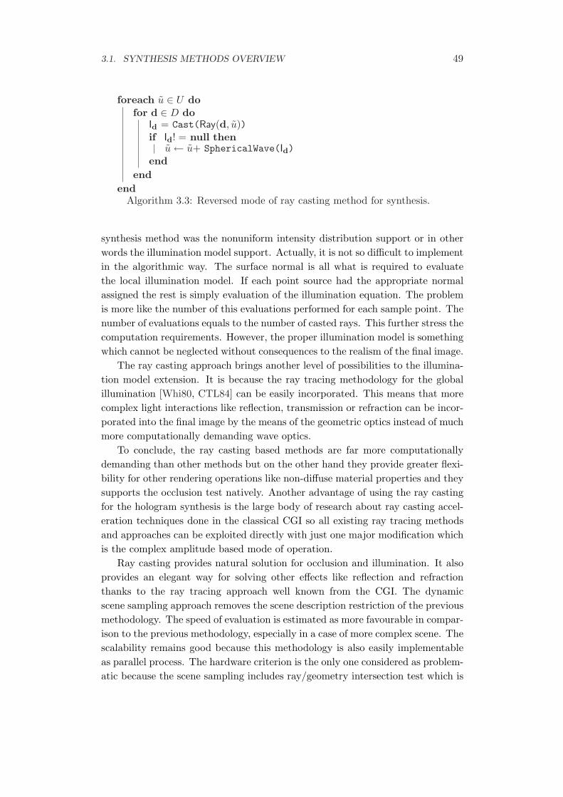
3.1. SYNTHESIS METHODS OVERVIEW 49
foreach u ∈ U dofor d ∈ D do
Id = Cast(Ray(d, u))if Id! = null then
u ← u+ SphericalWave(Id)end
endend
Algorithm 3.3: Reversed mode of ray casting method for synthesis.
synthesis method was the nonuniform intensity distribution support or in otherwords the illumination model support. Actually, it is not so difficult to implementin the algorithmic way. The surface normal is all what is required to evaluatethe local illumination model. If each point source had the appropriate normalassigned the rest is simply evaluation of the illumination equation. The problemis more like the number of this evaluations performed for each sample point. Thenumber of evaluations equals to the number of casted rays. This further stress thecomputation requirements. However, the proper illumination model is somethingwhich cannot be neglected without consequences to the realism of the final image.
The ray casting approach brings another level of possibilities to the illumina-tion model extension. It is because the ray tracing methodology for the globalillumination [Whi80, CTL84] can be easily incorporated. This means that morecomplex light interactions like reflection, transmission or refraction can be incor-porated into the final image by the means of the geometric optics instead of muchmore computationally demanding wave optics.
To conclude, the ray casting based methods are far more computationallydemanding than other methods but on the other hand they provide greater flexi-bility for other rendering operations like non-diffuse material properties and theysupports the occlusion test natively. Another advantage of using the ray castingfor the hologram synthesis is the large body of research about ray casting accel-eration techniques done in the classical CGI so all existing ray tracing methodsand approaches can be exploited directly with just one major modification whichis the complex amplitude based mode of operation.
Ray casting provides natural solution for occlusion and illumination. It alsoprovides an elegant way for solving other effects like reflection and refractionthanks to the ray tracing approach well known from the CGI. The dynamicscene sampling approach removes the scene description restriction of the previousmethodology. The speed of evaluation is estimated as more favourable in compar-ison to the previous methodology, especially in a case of more complex scene. Thescalability remains good because this methodology is also easily implementableas parallel process. The hardware criterion is the only one considered as problem-atic because the scene sampling includes ray/geometry intersection test which is
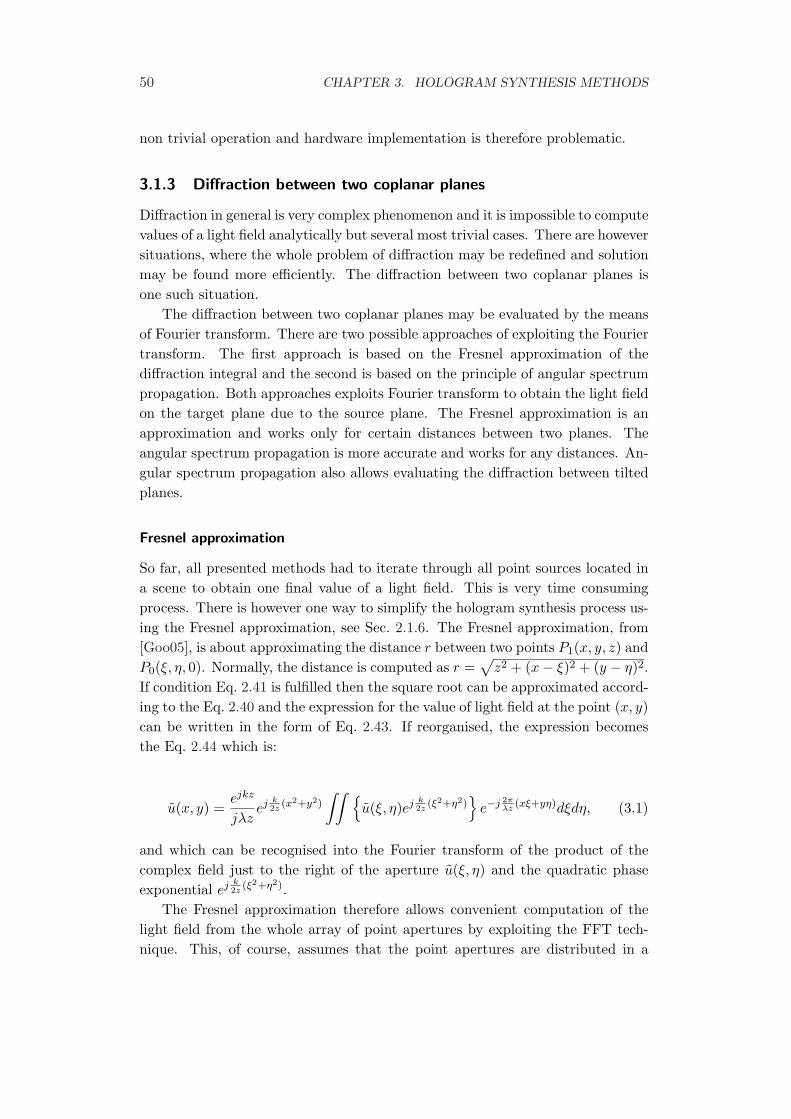
50 CHAPTER 3. HOLOGRAM SYNTHESIS METHODS
non trivial operation and hardware implementation is therefore problematic.
3.1.3 Diffraction between two coplanar planes
Diffraction in general is very complex phenomenon and it is impossible to computevalues of a light field analytically but several most trivial cases. There are howeversituations, where the whole problem of diffraction may be redefined and solutionmay be found more efficiently. The diffraction between two coplanar planes isone such situation.
The diffraction between two coplanar planes may be evaluated by the meansof Fourier transform. There are two possible approaches of exploiting the Fouriertransform. The first approach is based on the Fresnel approximation of thediffraction integral and the second is based on the principle of angular spectrumpropagation. Both approaches exploits Fourier transform to obtain the light fieldon the target plane due to the source plane. The Fresnel approximation is anapproximation and works only for certain distances between two planes. Theangular spectrum propagation is more accurate and works for any distances. An-gular spectrum propagation also allows evaluating the diffraction between tiltedplanes.
Fresnel approximation
So far, all presented methods had to iterate through all point sources located ina scene to obtain one final value of a light field. This is very time consumingprocess. There is however one way to simplify the hologram synthesis process us-ing the Fresnel approximation, see Sec. 2.1.6. The Fresnel approximation, from[Goo05], is about approximating the distance r between two points P1(x, y, z) andP0(ξ, η, 0). Normally, the distance is computed as r =
√z2 + (x− ξ)2 + (y − η)2.
If condition Eq. 2.41 is fulfilled then the square root can be approximated accord-ing to the Eq. 2.40 and the expression for the value of light field at the point (x, y)can be written in the form of Eq. 2.43. If reorganised, the expression becomesthe Eq. 2.44 which is:
u(x, y) =ejkz
jλzej k
2z(x2+y2)
∫∫ {u(ξ, η)ej k
2z(ξ2+η2)
}e−j 2π
λz(xξ+yη)dξdη, (3.1)
and which can be recognised into the Fourier transform of the product of thecomplex field just to the right of the aperture u(ξ, η) and the quadratic phaseexponential ej k
2z(ξ2+η2).
The Fresnel approximation therefore allows convenient computation of thelight field from the whole array of point apertures by exploiting the FFT tech-nique. This, of course, assumes that the point apertures are distributed in a

3.1. SYNTHESIS METHODS OVERVIEW 51
regular orthogonal grid. A method that utilise this Fresnel approximation forcomputing a hologram was published in [LHJ68].
The scene has to consist of point sources placed in three dimensional regulargrid. Each point has an intensity assigned. The scene can be therefore describedusing a set of grayscale images of the same size. The black color represents zeroamplitude and white color represents the largest amplitude allowed, see Fig. 3.1.3.Each image is then transformed into an array of complex amplitudes.
Figure 3.3: The scene consists of planar regular arrays of point apertures. Thedistance of the last array to the hologram is not in scale.
The following processing is based on the Eq. 3.1. Which means that eachtwo dimensional stack of points having the same z coordinate is multiplied bythe quadratic phase exponential ej k
2z(ξ2+η2) and FFT of the product is evaluated.
This operation constitutes the inner part of the Eq. 3.1.The result of FFT is then multiplied by the last exponential located in front
of the integral in Eq. 3.1 and the product is accumulated into the resulting lightfield of the hologram frame. The process is repeated for all images of the scenegrid. The particular hologram is then obtained as usual by adding the referencebeam and computing the intensity. The whole process may be therefore expressedas the Alg. 3.4.
To conclude, this approach is very fast in comparison with the point wiseor ray casting evaluation, the speed of evaluation criterion is therefore fulfilledsatisfactorily. On the other hand, the photorealism criterion is not fulfilled. Themost serious reason for the failure is the neglection of the occlusion. Each XYstack of the scene grid is processed absolutely independently on all others. Thepoint sources at the stacks farther from the hologram plane are always visible,even though they shouldn’t be. Another reason of the failure is the lack ofillumination model support. The point sources emit their energy uniformly to all
52 CHAPTER 3. HOLOGRAM SYNTHESIS METHODS
// QuadExp represents ej k2z
(ξ2+η2)
// Operator ⊗ represents element wise matrix multiplicationforeach Iz ∈ S do
I ′z ← QuadExp(z) ⊗ Iz
I ′′z ← FFT(I ′z)u ← u+QuadExp(z) ⊗ I ′′z
endAlgorithm 3.4: Fresnel approximation based synthesis method.
directions. This is enforced by the mathematics of the methodology and there isno resort to this issue.
Problematic is also the scene description since it is limited onto planar rect-angular elements coplanar with the hologram plane. The quality of hardwareimplementation is as good as is the quality of FFT implementation, which isnot as efficient as it is needed for the purposes of digital hologram synthesis.The scalability criterion is fulfilled satisfactorily because this methodology canbe implemented as parallel process.
Angular spectrum propagation
The synthesis methods based on the angular spectrum propagation, see Sec. 2.1.6are very similar to the methods described in the previous Sec. 3.1.3. The differ-ence between the Fresnel approximation and angular spectrum propagation isthe approximation part. The angular spectrum propagation is not approxima-tion and therefore it does not impose any limitations on the spatial extend of thesource and the distance of propagation. Although the angular spectrum propa-gation provides exact solution it is only a little bit more complicated comparedwith the Fresnel approximation since the only additional principal step is theinverse Fourier transform at the end of the process, see Sec. 2.1.6 for details. Theapproaches based on the Fresnel approximation can be therefore enhanced by re-placing the Fresnel approximation based propagation with the angular spectrumpropagation. The algorithm for this method is listed as Alg. 3.5:
// PropagExp represents the propagation exponential// Operator ⊗ represents element wise matrix multiplicationforeach Iz ∈ S do
I ′z ← FFT(Iz)I ′′z ← PropagExp(z) ⊗ Iz
u ← u+ IFFT(I ′′z )endAlgorithm 3.5: Angular spectrum propagation based synthesis method.
An interesting application of the angular spectrum propagation was published

3.1. SYNTHESIS METHODS OVERVIEW 53
in [TB93]. Authors proposed a method for synthesising a hologram of a scenecomposed of not regular 3D grid but of an arbitrarily tilted planes. The core ofthe approach is the propagation between two tilted planes. The first one is someof the plane of the scene, and the other one is the hologram frame.
The angular spectrum decomposes the light field into individual frequencycomponents, each constituting a direction of propagation of a single planar wave.If those directions are rotated, the light field on a plane rotated to the originalone. This transformation therefore allows obtaining a light field due to the planeA on a plane B which is rotated and transformed by the means of the angularspectrum propagation.
I
H
B
A
z
z’
y
w
u
0
0’
θ
θ’
Figure 3.4: Geometry for the determination of the light diffracted by plane I ontohologram plane H. The angular spectra of virtual planes A and B are consideredfor this calculation [TB93].
According to the [TB93] two reference frames (0;x, y, z) and (0; ξ, η, ζ) areassumed. The angular spectrum A2(fξ, fη, 0) on the plane 2(ξ, η, 0) is calculatedfrom the knowledge of A1(fx, fy, 0) which is the spectrum on the plane 1(x, y, 0).Let M be the rotation matrix relating (x, y, z) to (ξ, η, ζ) and the frequencies(fx, fy, fz) to (fξ, fη, fζ):
54 CHAPTER 3. HOLOGRAM SYNTHESIS METHODS
(x, y, z)T = M (ξ, η, ζ)T (3.2)
(fξ, fη, fζ)T = MT (fx, fy, fz)
T (3.3)
where fz =(1/λ2 − f2
x − f2y
)1/2.The angular spectrum propagation states that:
A2(fξ, fη, fζ) =
{0
A1(fx, fy, 0)fz/fζ(3.4)
The propagation is valid only if fz > 0 ∧ fζ > 0.The model of evaluating the diffraction pattern on any plane rotated and
translated with respect to the source plane is illustrated in the Fig. 3.4 whereonly rotations about x axes are shown. The plane I with a transmittance T (x, y)is illuminated by a monochromatic plane wave propagating in the direction u.The goal is to compute the diffraction pattern on the hologram plane H. It isdone in the following approach.
The diffraction pattern u(x, y) immediately behind the plane I is obtainedfrom the expression:
u(x, y) = T (x, y) exp(i2πy cos θ/λ), (3.5)
where θ is the angle between the y axis and the direction u. The Fourier trans-form of u(x, y) follows and the angular spectrum of I is obtained. The planeA is considered perpendicular to the auxiliary optical axis z′, which links thebarycenters 0 and 0′ of planes I and H respectively. A rotation transformationbetween the spectra of the planes I and A is done by exploiting the Eq. 3.3. Thetranslation is accomplished by the angular spectrum propagation and the spec-trum of the plane B is obtained. Another rotation transformation is executedbetween planes B and H thus the angular spectrum of the H is obtained. Thisis followed by the inverse Fourier transform of the angular spectrum which yieldthe diffraction pattern at the hologram plane H.
The process just described is repeated for all planes constituting the sceneand their contribution is accumulated to the final diffraction pattern. The par-ticular hologram is then obtained by adding the reference beam and evaluatingthe intensity. The algorithm for this method is listed as Alg. 3.6.
To conclude, although the angular spectrum based propagation is fast toevaluate and provides exact solution, it suffers by the same drawbacks describedin the previous section. It is unable to handle occlusion and more advancedillumination models. This greatly reduces it’s value as a hologram synthesisapproach. It is however a great tool for numerical reconstructions from light fielddue to the accuracy of propagation between two coplanar planes.

3.1. SYNTHESIS METHODS OVERVIEW 55
// PropagExp represents the propagation exponential// Operator ⊗ represents element wise matrix multiplicationforeach Iz ∈ S do
I ′z ← FFT(Iz)Rz ← RotateSpectrum(I ′z)R′
z ← PropagExp(z) ⊗ Rz
I ′′z ← RotateSpectrum(R′z)
u ← u+ IFFT(I ′′z )end
Algorithm 3.6: Light field of arbitrarily tilted planes computation exploitingangular spectrum rotation and propagation.
Less problematic is the scene description since it is not limited to coplanarrectangular elements only. Elements can be arbitrarily tilted. This allows align-ing each such plane with a triangle or planar polygon of the triangular mesh.The quality of hardware implementation is as good as is the quality of FFT im-plementation, which is not as efficient as it is needed for the purposes of digitalhologram synthesis. The scalability criterion is fulfilled satisfactorily because thismethodology can be implemented as parallel process.
3.1.4 Fourier hologram synthesis
Fourier holograms are a special kind of holograms, see Sec. 2.2.4 for details. Theyare special in the principle of recording. Both the reference and object beamsare projected by a lens first before they hit the hologram frame. The lens issituated such that the reference point light source and object lies in one focalplane and the hologram plane incidents with the second focal plane of the lens.This is the optical equivalent of making the Fourier transform of the referenceand object beam first and the hologram is then obtained from the interference ofthose transforms. The lens is also required for reconstructing the image.
The Fourier holograms have a very convenient mathematical description whichallows using the signal processing approaches for their faster synthesis. One ofthe approaches was published in [LAR01, AR03]. Authors combines a set of sceneprojections by a special process, which is shown to be equivalent to the recordingof the Fourier hologram.
The input of their approach is a set of scene’s projections from various viewingangles. The viewing angles are not arbitrary but they are chosen in such way asit is illustrated in the Fig. 3.5. The viewpoint direction is parameterized by theangles φm and θm.
Each of the computed projections pmn(xp, yp) is multiplied by the exponentialterm exp[−i2πb(xp sinφm + yp sin θn)]. This product is then summed to get a
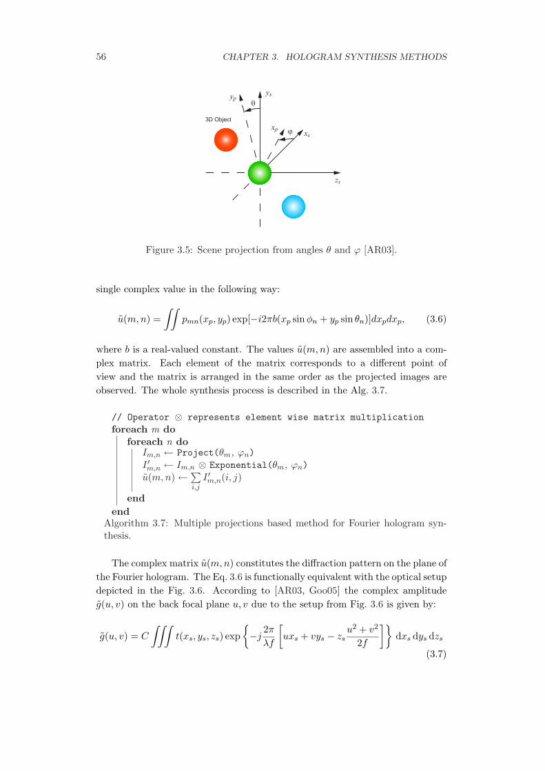
56 CHAPTER 3. HOLOGRAM SYNTHESIS METHODS
xp
ysyp
xs
zs
θ
ϕ
3D Object
Figure 3.5: Scene projection from angles θ and ϕ [AR03].
single complex value in the following way:
u(m,n) =∫∫
pmn(xp, yp) exp[−i2πb(xp sinφn + yp sin θn)]dxpdxp, (3.6)
where b is a real-valued constant. The values u(m,n) are assembled into a com-plex matrix. Each element of the matrix corresponds to a different point ofview and the matrix is arranged in the same order as the projected images areobserved. The whole synthesis process is described in the Alg. 3.7.
// Operator ⊗ represents element wise matrix multiplicationforeach m do
foreach n doIm,n ← Project(θm, ϕn)I ′m,n ← Im,n ⊗ Exponential(θm, ϕn)u(m,n) ← ∑
i,jI ′m,n(i, j)
endend
Algorithm 3.7: Multiple projections based method for Fourier hologram syn-thesis.
The complex matrix u(m,n) constitutes the diffraction pattern on the plane ofthe Fourier hologram. The Eq. 3.6 is functionally equivalent with the optical setupdepicted in the Fig. 3.6. According to [AR03, Goo05] the complex amplitudeg(u, v) on the back focal plane u, v due to the setup from Fig. 3.6 is given by:
g(u, v) = C
∫∫∫t(xs, ys, zs) exp
{−j
2π
λf
[uxs + vys − zs
u2 + v2
2f
]}dxs dys dzs
(3.7)
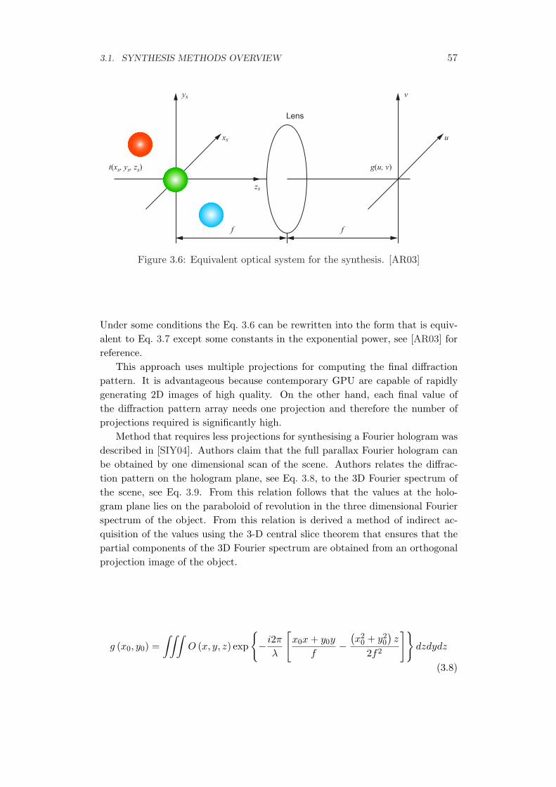
3.1. SYNTHESIS METHODS OVERVIEW 57
t(xs, ys, zs) g(u, v)
f f
Lens
ys
xs
zs
v
u
Figure 3.6: Equivalent optical system for the synthesis. [AR03]
Under some conditions the Eq. 3.6 can be rewritten into the form that is equiv-alent to Eq. 3.7 except some constants in the exponential power, see [AR03] forreference.
This approach uses multiple projections for computing the final diffractionpattern. It is advantageous because contemporary GPU are capable of rapidlygenerating 2D images of high quality. On the other hand, each final value ofthe diffraction pattern array needs one projection and therefore the number ofprojections required is significantly high.
Method that requires less projections for synthesising a Fourier hologram wasdescribed in [SIY04]. Authors claim that the full parallax Fourier hologram canbe obtained by one dimensional scan of the scene. Authors relates the diffrac-tion pattern on the hologram plane, see Eq. 3.8, to the 3D Fourier spectrum ofthe scene, see Eq. 3.9. From this relation follows that the values at the holo-gram plane lies on the paraboloid of revolution in the three dimensional Fourierspectrum of the object. From this relation is derived a method of indirect ac-quisition of the values using the 3-D central slice theorem that ensures that thepartial components of the 3D Fourier spectrum are obtained from an orthogonalprojection image of the object.
g (x0, y0) =∫∫∫
O (x, y, z) exp
{− i2π
λ
[x0x + y0y
f−
(x2
0 + y20
)z
2f2
]}dzdydz
(3.8)

58 CHAPTER 3. HOLOGRAM SYNTHESIS METHODS
g (u, v) =∫∫∫
O (x, y, z) exp{−i2π
[ux + vy − λ
2(u2 + v2
)z
]}dxdydz
={∫∫∫
O (x, y, z) exp [−i2π (ux + vy + wz)] dxdyd
}∣∣∣∣w=−λ(u2+v2)/2
= F [O (x, y, z)]|w=−λ(u2+v2)/2
(3.9)
At first, the object is projected onto a plane whose normal vector is inclinedby θ to the Z axis. Subsequently, the projected image is 2D Fourier transformed.The 2-D Fourier transform corresponds with a sectional Fourier plane whosenormal vector is also inclined by θ to the W axis in the 3-D Fourier space of theobject. Therefore, it is possible to obtain partial components on the paraboloidof revolution in Eq. 3.9 from one projection image using this principle.
x
y
z
u
v
w
(a) (b)
θθ
Figure 3.7: (a) Orthogonal projection in the real space and (b) a sectional planein the 3-D Fourier space obtained from a projection image. [SIY04]
However, only the intersection between the sectional Fourier plane and theparaboloid of revolution can be extracted from the sectional Fourier plane, seeFig. 3.8. The intersections are calculated from the equation of the sectional planeand the equation of the paraboloid of revolution, see Fig. 3.8. The solution ofthese equation is an ellipse, see Eq. 3.10. When projected onto the u-v plane,the ellipse becomes a circle with radius tan θ/λ. The position of the centre of thecircle depends on the direction of projection.
(u− tan θ
λ
)2
+ v2 =(
tan θ
λ
)2
, w = −u tan θ (3.10)
To obtain all coefficients on the u-v plane many circles has to be extracted insuch way that they fill the whole plane. The authors proposed a circular scanning
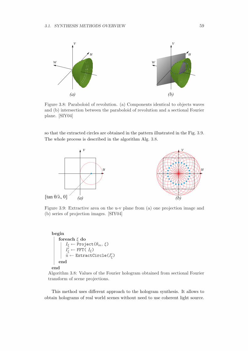
3.1. SYNTHESIS METHODS OVERVIEW 59
u
v
w
u
v
w
(a) (b)
Figure 3.8: Paraboloid of revolution. (a) Components identical to objects wavesand (b) intersection between the paraboloid of revolution and a sectional Fourierplane. [SIY04]
so that the extracted circles are obtained in the pattern illustrated in the Fig. 3.9.The whole process is described in the algorithm Alg. 3.8.
u
v
u
v
(a) (b)[tan θ/λ, 0]
Figure 3.9: Extractive area on the u-v plane from (a) one projection image and(b) series of projection images. [SIY04]
beginforeach ξ do
Iξ ← Project(θm, ξ)I ′ξ ← FFT( Iξ)u ← ExtractCircle(I ′ξ)
endend
Algorithm 3.8: Values of the Fourier hologram obtained from sectional Fouriertransform of scene projections.
This method uses different approach to the hologram synthesis. It allows toobtain holograms of real world scenes without need to use coherent light source.
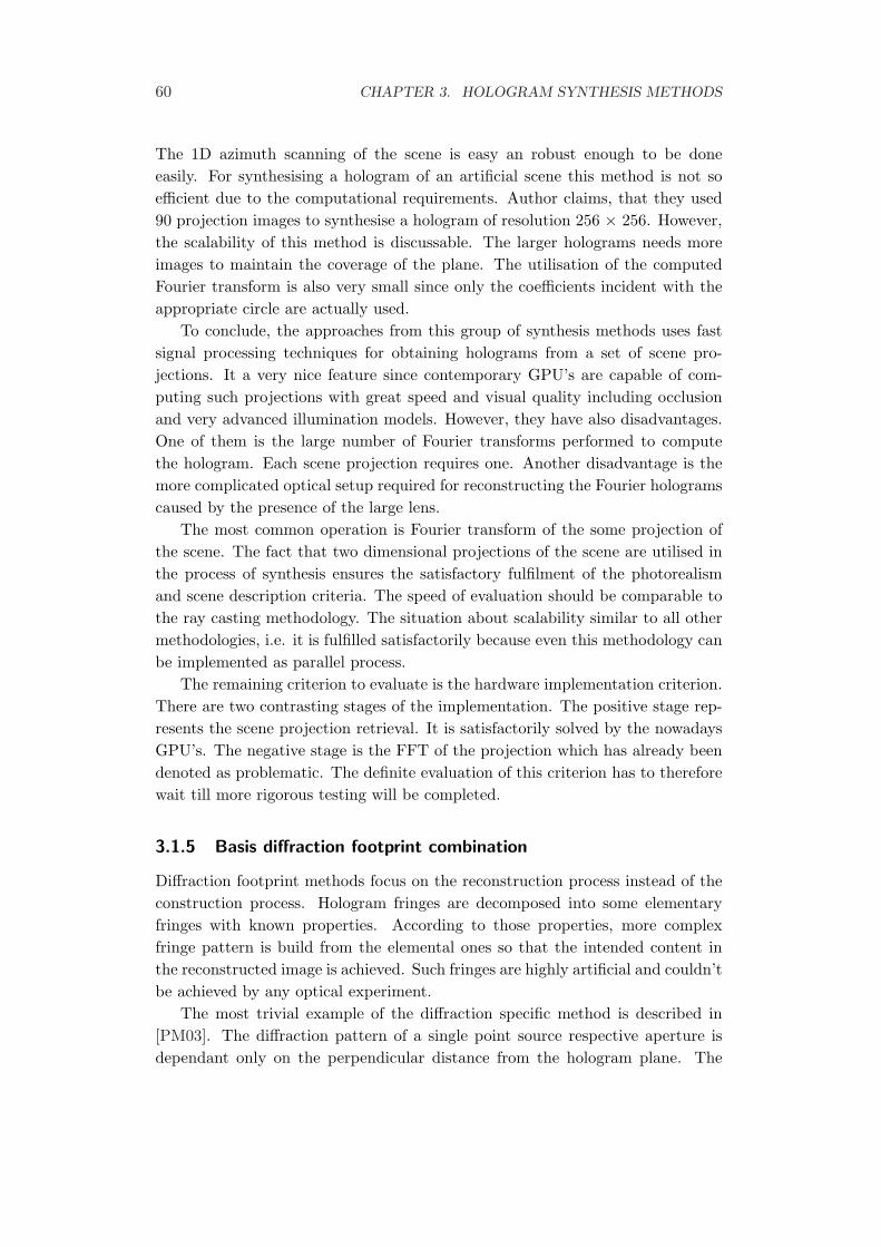
60 CHAPTER 3. HOLOGRAM SYNTHESIS METHODS
The 1D azimuth scanning of the scene is easy an robust enough to be doneeasily. For synthesising a hologram of an artificial scene this method is not soefficient due to the computational requirements. Author claims, that they used90 projection images to synthesise a hologram of resolution 256 × 256. However,the scalability of this method is discussable. The larger holograms needs moreimages to maintain the coverage of the plane. The utilisation of the computedFourier transform is also very small since only the coefficients incident with theappropriate circle are actually used.
To conclude, the approaches from this group of synthesis methods uses fastsignal processing techniques for obtaining holograms from a set of scene pro-jections. It a very nice feature since contemporary GPU’s are capable of com-puting such projections with great speed and visual quality including occlusionand very advanced illumination models. However, they have also disadvantages.One of them is the large number of Fourier transforms performed to computethe hologram. Each scene projection requires one. Another disadvantage is themore complicated optical setup required for reconstructing the Fourier hologramscaused by the presence of the large lens.
The most common operation is Fourier transform of the some projection ofthe scene. The fact that two dimensional projections of the scene are utilised inthe process of synthesis ensures the satisfactory fulfilment of the photorealismand scene description criteria. The speed of evaluation should be comparable tothe ray casting methodology. The situation about scalability similar to all othermethodologies, i.e. it is fulfilled satisfactorily because even this methodology canbe implemented as parallel process.
The remaining criterion to evaluate is the hardware implementation criterion.There are two contrasting stages of the implementation. The positive stage rep-resents the scene projection retrieval. It is satisfactorily solved by the nowadaysGPU’s. The negative stage is the FFT of the projection which has already beendenoted as problematic. The definite evaluation of this criterion has to thereforewait till more rigorous testing will be completed.
3.1.5 Basis diffraction footprint combination
Diffraction footprint methods focus on the reconstruction process instead of theconstruction process. Hologram fringes are decomposed into some elementaryfringes with known properties. According to those properties, more complexfringe pattern is build from the elemental ones so that the intended content inthe reconstructed image is achieved. Such fringes are highly artificial and couldn’tbe achieved by any optical experiment.
The most trivial example of the diffraction specific method is described in[PM03]. The diffraction pattern of a single point source respective aperture isdependant only on the perpendicular distance from the hologram plane. The

3.1. SYNTHESIS METHODS OVERVIEW 61
change of the diffraction pattern due to this distance manifests as a scale of thepattern. The diffraction pattern of a point can be therefore precomputed intoa complex texture once, see Fig. 3.10 and the diffraction patterns of any otherpoint within a scene can be obtained as a translation and a scale operation of thebasis texture which is easily done on a modern GPU’s.
Figure 3.10: Two components of a complex texture representing diffraction foot-print of a single point radiator. Imaginary component on the right and realcomponent on the left.
The scale operation that simulates shift in the perpendicular distance isnon-linear. If Dd represents the precomputed diffraction pattern at the dis-tance d then the scale factor s for diffraction pattern at the distance d′ will bes =
√(d′ + 0.5λ)/(d + 0.5λ). The λ is very small compared to the distances and
can be therefore neglected and the scale factor becomes s =√
d′/d. The approx-imation is sufficiently accurate for some range of distance from the precomputeddistance. The precomputed distance should be therefore chosen according tothe spatial extend of a scene. The best distance to choose is the centre of thebounding box of the scene.
The translation operation changes the position of a point radiator accordingto the X and Y axes. The parameters of the translation operation are chosensuch that the centre of the basis diffraction texture coincides with the positionof the point radiator. It is obvious that the basis textures has to be sufficientlylarge to cover the whole target frame for all combinations of translation and scalethat may occur for a given scene. The whole process of synthesis is simple andit is listed in the Alg 3.9.
This approach can be extended into more complex primitives. Diffractionpatterns of a finite line has been used in [RBD+99] and [FLB86]. The sameprinciple of transforming texture of an elemental diffraction pattern accordingto the spatial attributes of a primitive is used there. The diffraction pattern of
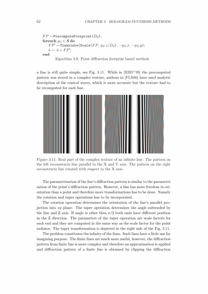
62 CHAPTER 3. HOLOGRAM SYNTHESIS METHODS
FP ←PrecomputeFootprint(Dd);foreach pS ∈ S do
FP ′ ←Translate(Scale(FP , pS .z/Dd), −pS .x, −pS .y);u ← u + FP ′;
endAlgorithm 3.9: Point diffraction footprint based method.
a line is still quite simple, see Fig. 3.11. While in [RBD+99] the precomputedpattern was stored in a complex texture, authors in [FLB86] have used analyticdescription of the conical waves, which is more accurate but the texture had tobe recomputed for each line.
Figure 3.11: Real part of the complex texture of an infinite line. The pattern onthe left reconstructs line parallel to the X and Y axis. The pattern on the rightreconstructs line rotated with respect to the X axis.
The parametrisation of the line’s diffraction pattern is similar to the parametri-sation of the point’s diffraction pattern. However, a line has more freedom in ori-entation than a point and therefore more transformations has to be done. Namelythe rotation and taper operations has to be incorporated.
The rotation operation determines the orientation of the line’s parallel pro-jection into xy plane. The taper operation determines the angle subtended bythe line and Z axis. If angle is other then π/2 both ends have different positionin the Z direction. The parameters of the taper operation are scale factors foreach end and they are computed in the same way as the scale factor for the pointradiator. The taper transformation is depicted in the right side of the Fig. 3.11.
The problem constitutes the infinity of the lines. Such lines have a little use forimagining purpose. The finite lines are much more useful, however, the diffractionpattern from finite line is more complex and therefore an approximation is appliedand diffraction pattern of a finite line is obtained by clipping the diffraction

3.1. SYNTHESIS METHODS OVERVIEW 63
pattern of an infinite line to the length of the line. This approximation causesblurring of the ends of a reconstructed line but tests proved this blurring feasibleunder certain conditions.
There is another problem with the clipping of the diffraction pattern. If lineis short, the diffraction pattern will be inherently short as well. This means thatthe diffraction pattern will not cover the whole hologram frame. This has twounpleasant consequences. First, the intensity of the reconstructed line is propor-tional to the relative area covered by the corresponding diffraction pattern. Theshorter the line is then less intense its reconstruction will be. And second, by notcovering the whole hologram plane with the diffraction pattern, the correspond-ing reconstructed line will be visible only from certain viewpoints. Therefore,also the viewing area of a single line is directly influenced by the relative area acorresponding diffraction pattern covers.
All the problems noted above constitute significant drawback in exploitingline primitive as basic building block. More useful primitive would be a triangle.Most common description of a geometry is by a triangular mesh. Thus havinga method for combining parametrised diffraction pattern texture of a trianglewould be most convenient. An attempt for employing diffraction pattern of atriangle as the basic diffractive primitives is presented in [KDS01].
The diffraction pattern of a triangle is not universal, i.e. the diffraction pat-tern of an arbitrary triangle is not obtained as a simple transformation of theprecomputed one. Therefore authors decided to precompute patterns for a tri-angle at different depths and different rotation angles. The synthesis algorithmtherefore requires a huge lookup table parameterized by the depth and rotation ofthe triangle. Diffraction pattern texture for a triangle is depicted in the Fig. 3.12and algorithm is summarised in Alg. 3.10.
Figure 3.12: Complex texture for a triangle. The real part is on the left andimaginary part is on the right.

64 CHAPTER 3. HOLOGRAM SYNTHESIS METHODS
// d - depth// ξ and η - rotation anglesTd,ξ,η ←PrecomputeFootprints();foreach Tri ∈ S do
P ← Td,ξ,η(Trid, T riξ, T riη);u ← u + P ;
endAlgorithm 3.10: Triangle diffraction footprint based method.
To conclude, the diffraction specific approaches try to reduce the complexityof the synthesis problem by focusing on the reconstruction output. If output con-forms with the correct image, then the synthesised hologram is all right althoughthe fringes are not physically correct according to the physics of the diffractionprocess. The approaches also exploits similar operations done by GPU’s whosesupport is often incorporated into the implementation. But the diffraction foot-print methods also have some serious drawbacks. One of them is the omnipresentproblem of occlusion. The elemental patterns are precomputed as completely vis-ible. Therefore, superposition of such element cannot yield an occluded surface.Another drawback is closely connected to the previous one. The basis elementsare precomputed from a surface having a uniform intensity. As a result, no varia-tion on the surface can be simulated. This makes the reconstructed image ratherbland. Both problems haven’t got straightforward solution which somewhat nul-lify the advertised speedup.
The basis diffraction footprint combination is very unbalanced methodology.It performs excellently in the speed of evaluation criterion, have a straightfor-ward hardware implementation, is scalable and have no problem with the scenedescription criterion but on the other hand it performs terribly in the photore-alism criterion. The methodology has difficulties in incorporating the occlusionsolution and illumination into the process of hologram synthesis.
Although, the most important criterion of photorealism is completely failed itis still a subject of continuous research. If a solution for photorealism support isfound without disrupting the outcome of the remaining criteria, this methodologybecomes the one with the most potential.
3.1.6 HPO holograms synthesis methods
A hologram is very redundant. It is useful for the quality of the image but itburdens the synthesis with massive calculation requirements. One way of speed-ing up the synthesis process is therefore omitting some significant part of theredundancy and horizontal parallax only holograms do exactly that. The HPOhologram exhibit only the horizontal parallax and lacks the vertical one com-pletely. This reduces the complexity of the synthesis by one order of magnitude.
3.1. SYNTHESIS METHODS OVERVIEW 65
The lack of vertical parallax is not so important as the horizontal one. It isbecause the human eyes are organised horizontally, thus the viewer does expe-rience the binocular disparity in the HPO hologram, hence she does sense thedepth. The drawback of HPO holograms is the necessity of a special reconstruc-tion setup composed of cylindrical lenses [LAR01], otherwise the reconstructedimage is heavily vertically blurred.
One of the greatest progress in the area of HPO hologram synthesis was doneat Massachusetts institute of technology - MIT Media Lab, where the SpatialImaging Group created a holographic system called Holovideo Display System.There are several approaches to digital HPO hologram synthesis that were tai-lored for this holographic device. They are summarised in the following sections.
MIT Holovideo Display System
The fundamental work about hologram synthesis for the MIT Holovideo deviceis described in [Luc94]. The fundamental contribution of this method is its ca-pability of achieving interactive rate of synthesis. The interactivity was achievedby significant reduction of hologram redundancy, which is generally too high tobe meaningfully utilised by human visual system. The complexity reduction isachieved by several factors.
First of all, the vertical parallax was sacrificed for reducing the dimension ofthe problem. Holograms without vertical parallax are commonly called horizontalparallax only or HPO holograms. HPO holograms are actually a vertical stackof one dimensional holograms which are much easier to synthesise. Also, verticalresolution of an HPO hologram can be much smaller than the horizontal one.
The disadvantage of HPO hologram is the need of special reconstruction setup[LAR01]. In a case of Holovideo system, this special reconstruction setup wasreplaced by the scanning process, where HPO hologram rows are processed se-quentially. The final image is then perceived as a whole because of the persistenceof vision.
Having the HPO hologram to synthesise instead of a full parallax one is notenough to achieve interactive frame rates. Further simplification is achieved bydiscretising the continuous signal of the hologram’s fringe pattern. This dicreti-sation is motivated by the limited capabilities of the human visual system – HVS.Hologram in general provides more information then HVS is capable to processand therefore the hologram signal can be discretised without apparent degrada-tion of the visual plausibility.
Let S (x, f) represents the spatial spectrum of a single line of a hologram.This spectrum is continuous for a real hologram, but it is not necessary fromthe HVS point of view. According to the sampling theorem, the signal has tobe sampled at least with two times higher frequency than the highest frequencycontained in signal. In this case the sampling frequency should be two times
66 CHAPTER 3. HOLOGRAM SYNTHESIS METHODS
higher then the highest frequency usable by the HVS. This highest frequencyshould be found for both x and f .
First, for a given spatial frequency f0, the spatial sampling spacing wh in x
must be small enough so that the most rapid amplitude variations in S (x, f0)can be reconstructed. Let the smallest variation in an image the HVS can see isset to 1 minute of an arc which is approximately 290 microradians. Consideringa typical viewing distance 60 cm then the wh is simply 0.000290×0.6 = 0.000174m.
Second, for a given fringe region wh centred at position x0 the spatial fre-quency sample spacing ∆f must be sufficiently small to reconstruct the mostrapid variations in S (x0, f) as a function of f . The ability of the human eyeto detect view-dependent variations is limited by the size of the pupil which istypically 3 mm. The angle subtended by the human pupil therefore determinesthe maximum allowable ∆f . It can be computed from the diffraction gratingequation Eq. 2.51 which can also be written as:
sin θq (λ)− sin θi = qλf, (3.11)
where f denotes the spatial frequency of the grating, λ denotes wavelength, q
denotes diffracted order (can be negative), θq denotes the diffracted angle in theorder q and θi denotes the incident angle.
Let q = 1, which is the order of interest in holography, and θi = 0 then takingthe derivative of both sides with respect to θ1 one obtains:
df
dθ1=
cos θ1
λ. (3.12)
For a viewing distance of 600 mm and a λ = 0.633 µm the calculation of ∆f
becomes∆f =
(3mm) / (600mm)0.633µm
= 8mm−1. (3.13)
In a case of [Luc94], the fringe had width 1024 samples and each sample isspaced by 0.6 µm, the spatial frequencies therefore range from 0 to 850 mm−1
with spacing 0.8 mm−1, which ten times exceeds the computed ∆f . The fringecan be therefore encoded so that the bandwidth is compressed while useful imageinformation is preserved.
Having the discretisation specified the term hogel can be introduced. Hogelis a small region of a fringe pattern. In a case of HPO hologram, it constitutesa small line segment of width wh. Hogel is small enough to appear as a singlepoint to the viewer and represents sampling of S (x, f) at intervals of wh and ∆f
which means that the hogel is completely described by its spectrum.It was shown that diffracted light can be decomposed into a spectrum of
planar waves, see Sec. 3.1.3. For each direction exists a spatial frequency thatdiffracts light into that direction. The range of direction is divided into small
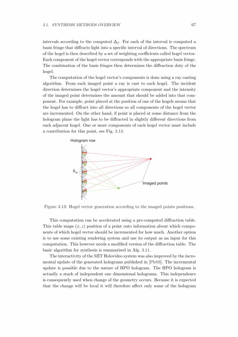
3.1. SYNTHESIS METHODS OVERVIEW 67
intervals according to the computed ∆f . For each of the interval is computed abasis fringe that diffracts light into a specific interval of directions. The spectrumof the hogel is then described by a set of weighting coefficients called hogel vector.Each component of the hogel vector corresponds with the appropriate basis fringe.The combination of the basis fringes then determines the diffraction duty of thehogel.
The computation of the hogel vector’s components is done using a ray castingalgorithm. From each imaged point a ray is cast to each hogel. The incidentdirection determines the hogel vector’s appropriate component and the intensityof the imaged point determines the amount that should be added into that com-ponent. For example, point placed at the position of one of the hogels means thatthe hogel has to diffract into all directions so all components of the hogel vectorare incremented. On the other hand, if point is placed at some distance from thehologram plane the light has to be diffracted in slightly different directions fromeach adjacent hogel. One or more components of each hogel vector must includea contribution for this point, see Fig. 3.13.
hw
Hologram row
Imaged points
Figure 3.13: Hogel vector generation according to the imaged points positions.
This computation can be accelerated using a pre-computed diffraction table.This table maps (x, z) position of a point onto information about which compo-nents of which hogel vector should be incremented for how much. Another optionis to use some existing rendering system and use its output as an input for thiscomputation. This however needs a modified version of the diffraction table. Thebasic algorithm for synthesis is summarised in Alg. 3.11.
The interactivity of the MIT Holovideo system was also improved by the incre-mental update of the generated holograms published in [Ple03]. The incrementalupdate is possible due to the nature of HPO hologram. The HPO hologram isactually a stack of independent one dimensional holograms. This independenceis consequently used when change of the geometry occurs. Because it is expectedthat the change will be local it will therefore affect only some of the hologram
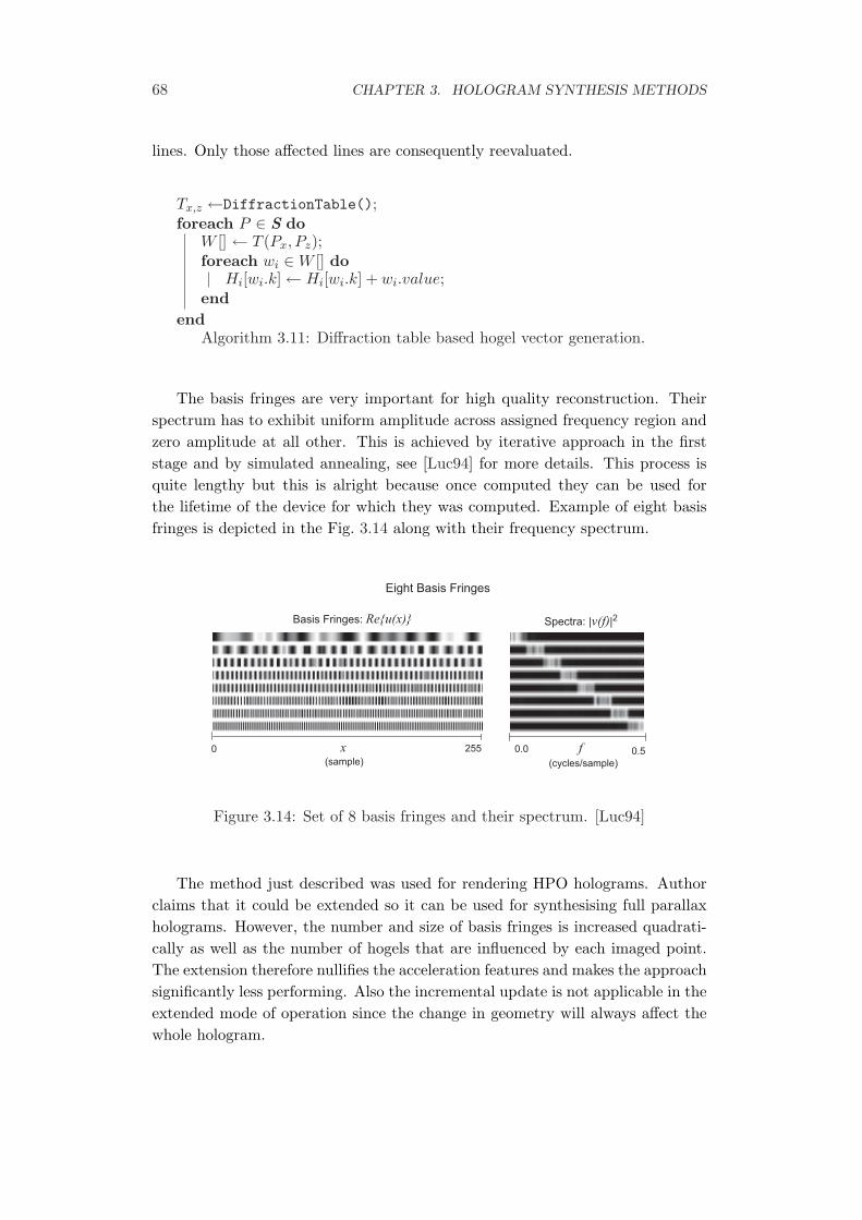
68 CHAPTER 3. HOLOGRAM SYNTHESIS METHODS
lines. Only those affected lines are consequently reevaluated.
Tx,z ←DiffractionTable();foreach P ∈ S do
W [] ← T (Px, Pz);foreach wi ∈ W [] do
Hi[wi.k] ← Hi[wi.k] + wi.value;end
endAlgorithm 3.11: Diffraction table based hogel vector generation.
The basis fringes are very important for high quality reconstruction. Theirspectrum has to exhibit uniform amplitude across assigned frequency region andzero amplitude at all other. This is achieved by iterative approach in the firststage and by simulated annealing, see [Luc94] for more details. This process isquite lengthy but this is alright because once computed they can be used forthe lifetime of the device for which they was computed. Example of eight basisfringes is depicted in the Fig. 3.14 along with their frequency spectrum.
0.0 0.5fx0 255
Basis Fringes: Re{u(x)} Spectra: |v(f)|2
(cycles/sample)(sample)
Eight Basis Fringes
Figure 3.14: Set of 8 basis fringes and their spectrum. [Luc94]
The method just described was used for rendering HPO holograms. Authorclaims that it could be extended so it can be used for synthesising full parallaxholograms. However, the number and size of basis fringes is increased quadrati-cally as well as the number of hogels that are influenced by each imaged point.The extension therefore nullifies the acceleration features and makes the approachsignificantly less performing. Also the incremental update is not applicable in theextended mode of operation since the change in geometry will always affect thewhole hologram.

3.1. SYNTHESIS METHODS OVERVIEW 69
Occlusion and shading support
The approach of M. Lucente was extended in [Und97]. The author augmented anocclusion solver into the Holovideo system and smooth shading was also incor-porated. The situation is much more simpler in a case of HPO hologram whenocclusion is discussed. The HPO hologram is a stack of horizontally orientedone dimensional holograms that do not interact with each other. The occlusionproblem is therefore reduced from three dimensions into two dimensions only.
The occlusion solver has to decide, if the currently processed point is capableof contributing to any of the hogels. If point does not contribute to any of thehogels because it is fully occluded, then it is completely rejected. The oppositecase where completely visible point contributes to all hogels is also easy since itis processed as described in the previous section. The more complicated case iswhen point contributes only to a subset of hogels. The information about hogelsthat are affected by the partially occluded point must be passed into next stageof the system, so that unaffected hogels are not processed.
To evaluate the occlusion, an auxiliary information is needed since Holovideoworks pointwise and point is too small to occlude anything. The auxiliary infor-mation is extracted from the original geometry that was used for populating theinput points. For each plane corresponding to the currently processed hologramline an intersection with the geometry is computed. This intersection produces aset of polygons respective line segments. Those segments constitutes the so calledobstructor mask against which input points from the same plane are tested.
Each point has to be tested against each part of the obstructor mask. Thisis rather complicated so two simpler tests are performed first. The first testchecks, if the processed point lies on the tested obstructor mask segment. If yes,then the segment is rejected from the following testing. The second test rejectsall obstructor mask’s line segments that have both endpoints farther from thehologram line then the precessed point and therefore cannot never occlude thepoint.
The further processing consists of computing the geometric shadow of eachsegment against the z = 0 plane. If any part of the projection lies within thehorizontal extend of the hologram then the projection added into the point sourcesoccluded interval, see Fig. 3.15. The final interval is kept as simple as possible soeach new interval is added logically.
In the end, each point has its occluded interval and can be passed into the nextstage of processing. Those points having occlusion interval which completely cov-ers the whole hologram line can be rejected right away. Other points contributeonly to those hogels, that do not fall into the occluded part of the occlusioninterval. The contributions are normally processed according to the diffractiontable as described in the previous section.
The last extension of the Holovide system authors of [Und97] described was

70 CHAPTER 3. HOLOGRAM SYNTHESIS METHODS
Hologram line
Processed point source
Obstructor mask
Occlusion interval
Figure 3.15: Occlusion interval determination [Und97].
shading and illumination. Both shading and illumination support is rather simpleone. The intensity is computed according to the illumination model, Phong’smodel in this case, and assigned into each point source as its amplitude. Thisis done also for the specular component, which is view dependant and should betherefore recomputed for each hogel influenced by the processed point. However,authors evaluated this approach as too computationally demanding and decidedto evaluate the specular component from one viewpoint and use that value forall hogels. The specular highlight is therefore static even though it should movealong the surface according to the viewer’s positon.
Conclusion
All synthesis methods dedicated to the MIT Holovideo system depend on thespecial features of the HPO hologram synthesis. Those special features, which areresponsible for the phenomenal efficiency of the whole system, would not persistif the Holovideo system was transformed to support the full parallax hologramsynthesis and reproduction. Therefore the significance of the methods describedin the Section 3.1.6 for the purposes of this work is reduced. However, some of theconcepts utilised in the HPO hologram synthesis are worth of incorporating intoother methodologies, e.g. the basis diffraction footprint combination methodologymay benefit from those concepts.
3.2 Summarisation and evaluation of the methods
The variation of the approaches for digital hologram synthesis is large. Thecommon characteristic is the tradeoff between the quality of the output and thecomputational demands. The fastest approaches are the least flexible ones andvice versa. When evaluating the eligibility of the methodology, the application ofthe synthesised holograms plays a great role in the process. Since the main goal ofthis work is high quality imaging then the most important feature is the supportfor photorealistic rendering and the secondary feature is of course the speed ofevaluation. However high quality and fast evaluation are in obvious contradiction.The advertised methods are therefore compared with respect to their ability to

3.2. SUMMARISATION AND EVALUATION OF THE METHODS 71
produce photorealistic output or their potential extensibility in this direction andtheir speed of evaluation. The overview of the synthesis methods’ parameters ispresented in the table A.1.
According to the results of evaluation, as the most eligible methods for thepurposes of this work were chosen these methods ordered by their eligibility:
1. Ray casting method of synthesis,
2. Fourier hologram synthesis,
3. Basis Diffraction footprint combination.
Ray casting was chosen as the best because it is capable of providing photore-alistic output. Although the core speed of evaluation is not so good the scalabilityof this method compensates that issue. And finally, the scene content descriptiondoes not require any additional information and standard description as usednowadays suffices. Successful hardware implementation also supports the choiceof this methodology.
Fourier hologram synthesis was chosen for its ability to produce photoreal-istic output. The most interesting feature of the Fourier hologram synthesis isits input which consists of a set of two dimensional projections of the synthe-sised scene. This even allows synthesising holograms from the images providedby charge-coupled device - CCD camera. The reason for being chosen as secondis necessity of more complex optical setup for reconstruction. Also the scalabil-ity and hardware implementation are more problematic than in the case of raycasting.
The basis diffraction footprint combination excels with the speed of evaluationand hardware support, however the realism of the output is in the current stateunsufficient. If the issue of realism is sufficiently solved then this approach willbecome very well performing and might compete with the previous two method-ologies. This approach was therefore also chosen to be included in the futureresearch.
From the evaluation is apparent that the MIT Holovide also performs su-perbly. However, its specialisation to HPO holograms may become unfeasiblein the future. The extension of the system into a full parallax supporting holo-graphic system will probably spoil all advantages and interactivity implied by theHPO hologram synthesis specifics. This is a reason, why this methodology wasnot chosen as perspective one.

Chapter 4
Proposed ray casting synthesis
method
Some work has already been done in the area of ray casting methodology forholograms synthesis. The ray casting was chosen as the core technology becauseit is closely related to the area of computer graphics and has a large body ofresearch at disposal. The problem of synthesis was restricted to HPO hologramsynthesis because of the computation complexity reduction. The reduced com-putation complexity implies shorter computation time and shorter computationtime allows more rapid development. The ray casting method is also flexibleenough to be extended to synthesise the full parallax holograms too.
Among the advantages of the proposed method belongs automatic processing,which doesn’t require any special input. The input of the method is the commonscene description including the triangular meshes together with material andlight specifications. The light type is restricted to directional light but only dueto the efficiency reasons. Any other light types, e.g. omnidirectional, spot, aresupported but for the cost of increased computation complexity. This supportfor common scene description is a very useful feature because it allows seamlessintegration of the synthesis method into the existing 3D content authoring toolslike 3D Studio Max.
The rest of the chapter deals with the description of the method, which hasalready been published in [JHS06c] and [JHS06a].
4.1 Basic principle
This section describes the proposed method for synthesising a hologram of atriangular mesh objects. This method is capable of evaluating an occlusion, i.e.a point is not considered if it is occluded by some other point and visibility,
73
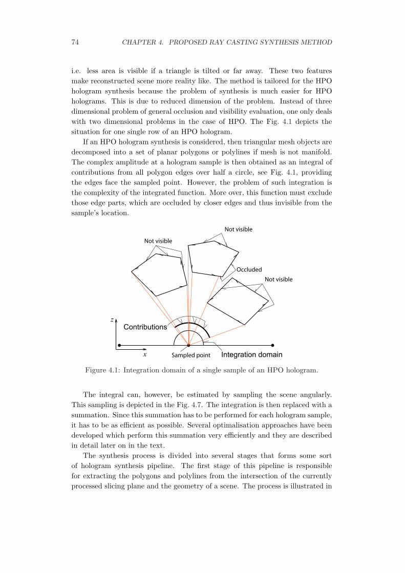
74 CHAPTER 4. PROPOSED RAY CASTING SYNTHESIS METHOD
i.e. less area is visible if a triangle is tilted or far away. These two featuresmake reconstructed scene more reality like. The method is tailored for the HPOhologram synthesis because the problem of synthesis is much easier for HPOholograms. This is due to reduced dimension of the problem. Instead of threedimensional problem of general occlusion and visibility evaluation, one only dealswith two dimensional problems in the case of HPO. The Fig. 4.1 depicts thesituation for one single row of an HPO hologram.
If an HPO hologram synthesis is considered, then triangular mesh objects aredecomposed into a set of planar polygons or polylines if mesh is not manifold.The complex amplitude at a hologram sample is then obtained as an integral ofcontributions from all polygon edges over half a circle, see Fig. 4.1, providingthe edges face the sampled point. However, the problem of such integration isthe complexity of the integrated function. More over, this function must excludethose edge parts, which are occluded by closer edges and thus invisible from thesample’s location.
Figure 4.1: Integration domain of a single sample of an HPO hologram.
The integral can, however, be estimated by sampling the scene angularly.This sampling is depicted in the Fig. 4.7. The integration is then replaced with asummation. Since this summation has to be performed for each hologram sample,it has to be as efficient as possible. Several optimalisation approaches have beendeveloped which perform this summation very efficiently and they are describedin detail later on in the text.
The synthesis process is divided into several stages that forms some sortof hologram synthesis pipeline. The first stage of this pipeline is responsiblefor extracting the polygons and polylines from the intersection of the currentlyprocessed slicing plane and the geometry of a scene. The process is illustrated in
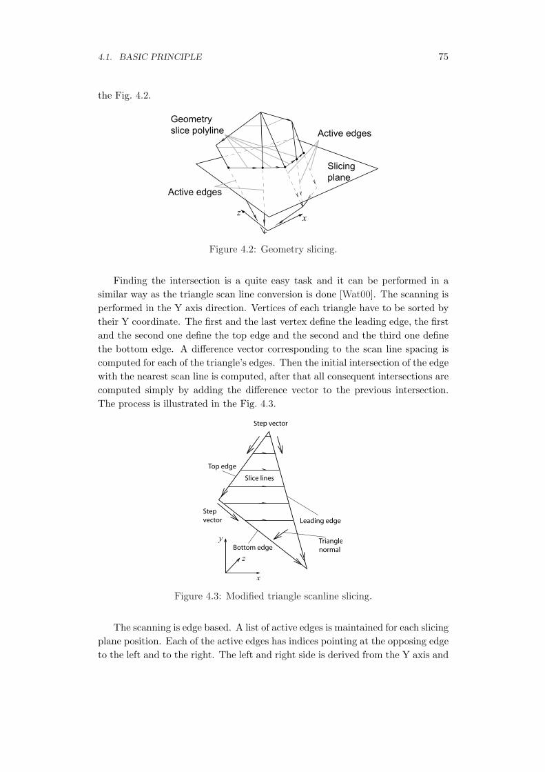
4.1. BASIC PRINCIPLE 75
the Fig. 4.2.
Active edges
Active edges
Slicing
plane
Geometry
slice polyline
xz
Figure 4.2: Geometry slicing.
Finding the intersection is a quite easy task and it can be performed in asimilar way as the triangle scan line conversion is done [Wat00]. The scanning isperformed in the Y axis direction. Vertices of each triangle have to be sorted bytheir Y coordinate. The first and the last vertex define the leading edge, the firstand the second one define the top edge and the second and the third one definethe bottom edge. A difference vector corresponding to the scan line spacing iscomputed for each of the triangle’s edges. Then the initial intersection of the edgewith the nearest scan line is computed, after that all consequent intersections arecomputed simply by adding the difference vector to the previous intersection.The process is illustrated in the Fig. 4.3.
Figure 4.3: Modified triangle scanline slicing.
The scanning is edge based. A list of active edges is maintained for each slicingplane position. Each of the active edges has indices pointing at the opposing edgeto the left and to the right. The left and right side is derived from the Y axis and

76 CHAPTER 4. PROPOSED RAY CASTING SYNTHESIS METHOD
the triangle’s normal. Singular triangles having the normal linearly dependentwith the Y axis do not contribute to the hologram at all and can be thereforeomitted.
When new edge is added into the list of active edges the integrity of theopposing edge indices must be checked. If the edge indexed by the new edge doesnot index the new edge back then the swap between the upper and lower edgehas occurred and the index in the opposing leading edge has to be corrected.
The slice of a triangle, which is a line, is determined from the intersectionpoints of the current scan line with the leading edge and the currently activeopposing edge. The acquired line is required to be oriented in such way thatits first vertex is on the left side and the second one on the right side. The leftrespective right side is derived from the triangle’s normal.
An easy way to find out if the leading edge determines the first or the secondvertex of a slice line is using some vector algebra. One has to compute a dotproduct of a triangle’s normal and a vector product of the leading edge and thetop edge considered as vectors. The sign of the dot product determines if thevertex obtained from the leading edge is the first one or the second one. Thismethod of course requires uniform orientation of all triangles.
For each scanline and each active edge a corresponding slice vertex is created.Then slice edges are generated using the opposing edge information. Since tri-angles are aware of their orientation the slice edges are all oriented from left toright. This orientation is exploited when visibility is evaluated, see below. Thevertices and edges from all objects are joined into a single list and passed into anext stage of the pipeline.
The complication at this stage constitutes the data structures required forstoring the data required for shading purposes like normals or texture coordinates.The data need to be interpolated form values stored in vertices. The first phaseof interpolation is performed during the geometry slicing stage. Each scannededge has a data record associated and the interpolated values are obtained in asame fashion as the computation of intersections described above. The differencecorresponding to the change in the Y component is computed in the initializationstep and the actual value of datum is obtained from the previous one simply byadding the difference. This process constitutes a linear interpolation.
Once the slice edges are obtained, the interpolated data values d are obtainedas d(l) = A + l(B −A) where A are data at the first vertex of a slice edge, B aredata at the second vertex of a slice edge, l is the interpolation parameter acquiredas l = LS/L, see Fig. 4.8. Difference (A−B) is stored in the slice edge.
The texture coordinates were mentioned as an example of interpolated data,but any other attributes can be added such as vertex colours. Normals are alsousually interpolated but the normals have to be renormalised, which is quitecostly operation. As an alternative, the normals can be taken from a normal

4.1. BASIC PRINCIPLE 77
map providing a texture fetch is faster than the normal normalisation.The result of the slicing is a set of oriented lines. The situation is depicted in
the Fig. 4.1. It is obvious that some of the lines are invisible from every samplepoint of the current row. The question is how to detect invisibility from a givenpoint. This is the part where line orientation comes into play.
The angles subtended by the join of the examined x sample at the hologramline and the respective endpoints of the line and the X axis are computed. Thevisibility of the line is then determined by simple comparison of the computedangles. See Fig. 4.4 for reference. If α angle is smaller than the β angle then theline is not visible from the point x.
Figure 4.4: Principle of visibility check.
The line is a potential contributor if it is visible from at least one of thehologram extremes. See Fig. 4.5 for reference. The lines that are invisible fromboth hologram extremes are removed because they never contribute. Everythingis set for the next, most computationally demanding phase, which is the angularsampling.
Figure 4.5: Candidate lines are those visible from at least one hologram rowextreme.
One more preprocessing task, which is the lines length computation, has tobe done. The direct distance computation, exploiting the square root operation,
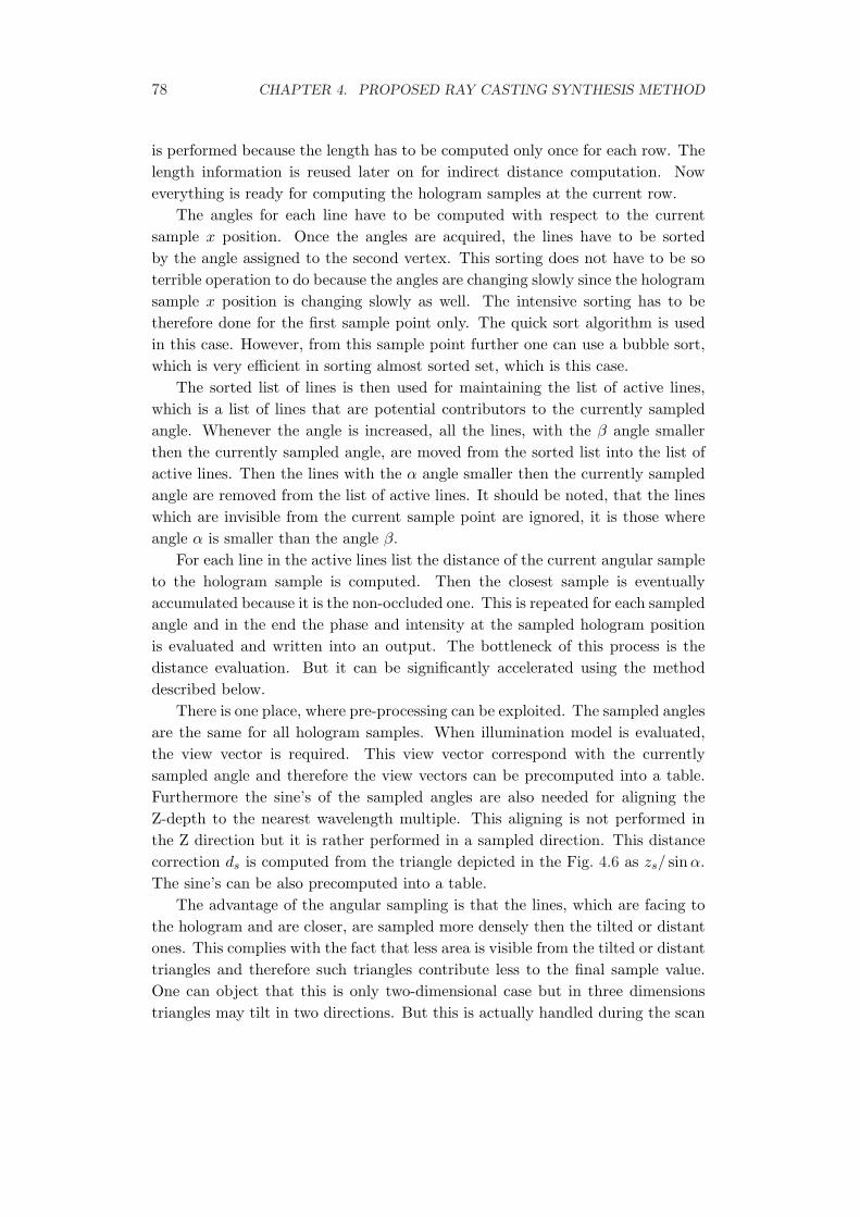
78 CHAPTER 4. PROPOSED RAY CASTING SYNTHESIS METHOD
is performed because the length has to be computed only once for each row. Thelength information is reused later on for indirect distance computation. Noweverything is ready for computing the hologram samples at the current row.
The angles for each line have to be computed with respect to the currentsample x position. Once the angles are acquired, the lines have to be sortedby the angle assigned to the second vertex. This sorting does not have to be soterrible operation to do because the angles are changing slowly since the hologramsample x position is changing slowly as well. The intensive sorting has to betherefore done for the first sample point only. The quick sort algorithm is usedin this case. However, from this sample point further one can use a bubble sort,which is very efficient in sorting almost sorted set, which is this case.
The sorted list of lines is then used for maintaining the list of active lines,which is a list of lines that are potential contributors to the currently sampledangle. Whenever the angle is increased, all the lines, with the β angle smallerthen the currently sampled angle, are moved from the sorted list into the list ofactive lines. Then the lines with the α angle smaller then the currently sampledangle are removed from the list of active lines. It should be noted, that the lineswhich are invisible from the current sample point are ignored, it is those whereangle α is smaller than the angle β.
For each line in the active lines list the distance of the current angular sampleto the hologram sample is computed. Then the closest sample is eventuallyaccumulated because it is the non-occluded one. This is repeated for each sampledangle and in the end the phase and intensity at the sampled hologram positionis evaluated and written into an output. The bottleneck of this process is thedistance evaluation. But it can be significantly accelerated using the methoddescribed below.
There is one place, where pre-processing can be exploited. The sampled anglesare the same for all hologram samples. When illumination model is evaluated,the view vector is required. This view vector correspond with the currentlysampled angle and therefore the view vectors can be precomputed into a table.Furthermore the sine’s of the sampled angles are also needed for aligning theZ-depth to the nearest wavelength multiple. This aligning is not performed inthe Z direction but it is rather performed in a sampled direction. This distancecorrection ds is computed from the triangle depicted in the Fig. 4.6 as zs/ sinα.The sine’s can be also precomputed into a table.
The advantage of the angular sampling is that the lines, which are facing tothe hologram and are closer, are sampled more densely then the tilted or distantones. This complies with the fact that less area is visible from the tilted or distanttriangles and therefore such triangles contribute less to the final sample value.One can object that this is only two-dimensional case but in three dimensionstriangles may tilt in two directions. But this is actually handled during the scan

4.1. BASIC PRINCIPLE 79
α
Closest multiple of λ
Sampled edge
Computed distance
zs
ds
Figure 4.6: Aligning of the Z-depth.
line conversion. Tilted triangles end up with less scan lines then those facing thehologram plane more directly.
This angular sampling also provides uniform sampling for the whole scene.As a result, one can use radiance values obtained from illumination model asthe amplitude value. And because the hologram is normalised at the end, theintensity distribution of a scene is maintained and it is independent on the angularsampling step. The angular sampling process is depicted in the Fig. 4.7
Angular step
Sampled point
z
x
Figure 4.7: Angular sampling of the slice geometry.
Edges in a slice are sampled using the sine law in a triangle. The triangleis depicted in the Fig. 4.8. The β angle is gradually decreased and the α angleis gradually increased as the sampled angle advances counter clock wise. Theα angle is used for recalculation of the triangle ratio. The γ angle is used forevaluation of the distance d and the β angle is used for evaluating the length LS
exploited for computing the parameter of a data record’s linear interpolation.The uniform change of the sampling angle is an advantage because the dif-
ferential equation for cosine evaluation can be used. This differential equation isbased on the well known reflection vector evaluation R = 2N (cosα) − L. Thecosine corresponds to the X coordinate of the reflection vector. The new cosinevalue is obtained from the two previous values as it is apparent form the Eq. 4.1[Has06]. The sine function can be computed similarly only a value of π/2 issubtracted from the initial angle.
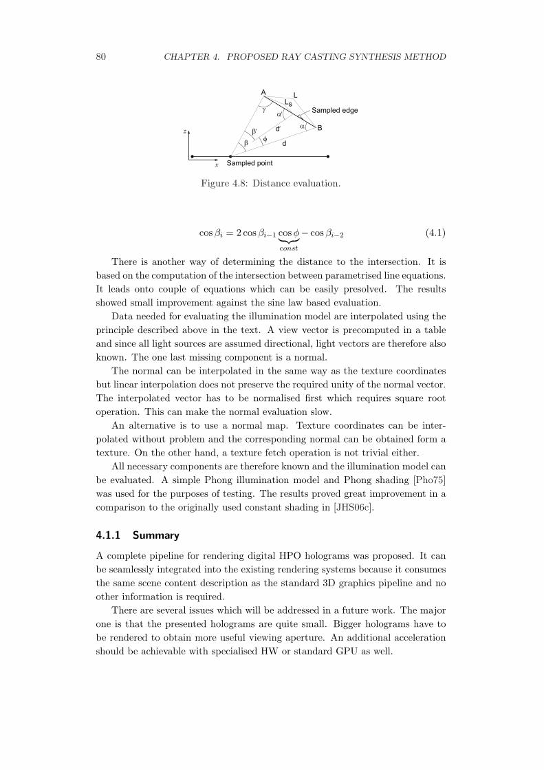
80 CHAPTER 4. PROPOSED RAY CASTING SYNTHESIS METHOD
φβ
β
LLs
α
α
γ
A
B
d
d
Sampled point
Sampled edge
Figure 4.8: Distance evaluation.
cosβi = 2 cosβi−1 cosφ︸ ︷︷ ︸const
− cosβi−2 (4.1)
There is another way of determining the distance to the intersection. It isbased on the computation of the intersection between parametrised line equations.It leads onto couple of equations which can be easily presolved. The resultsshowed small improvement against the sine law based evaluation.
Data needed for evaluating the illumination model are interpolated using theprinciple described above in the text. A view vector is precomputed in a tableand since all light sources are assumed directional, light vectors are therefore alsoknown. The one last missing component is a normal.
The normal can be interpolated in the same way as the texture coordinatesbut linear interpolation does not preserve the required unity of the normal vector.The interpolated vector has to be normalised first which requires square rootoperation. This can make the normal evaluation slow.
An alternative is to use a normal map. Texture coordinates can be inter-polated without problem and the corresponding normal can be obtained form atexture. On the other hand, a texture fetch operation is not trivial either.
All necessary components are therefore known and the illumination model canbe evaluated. A simple Phong illumination model and Phong shading [Pho75]was used for the purposes of testing. The results proved great improvement in acomparison to the originally used constant shading in [JHS06c].
4.1.1 Summary
A complete pipeline for rendering digital HPO holograms was proposed. It canbe seamlessly integrated into the existing rendering systems because it consumesthe same scene content description as the standard 3D graphics pipeline and noother information is required.
There are several issues which will be addressed in a future work. The majorone is that the presented holograms are quite small. Bigger holograms have tobe rendered to obtain more useful viewing aperture. An additional accelerationshould be achievable with specialised HW or standard GPU as well.
Chapter 5
Summary and Conclusion
The purpose of this STAR document was the following. First, present a compi-lation of pieces of knowledge regarding the holography science in general. Thiscompilation constitutes a supporting material for the synthesis method’s overviewand evaluation and furthermore, it may serve as a minimal knowledge pack usefulfor anyone, who wants to deal with holography.
Second, the overview and evaluation of the digital hologram synthesis meth-ods. This overview constitutes the starting point for the next work and devel-opment. It reflects the actual state in the area of digital hologram synthesis.The evaluation of the method’s features directly determines the direction of thefollowing direction of research. The first results of this research is included in theChapter 4.
And finally, the proposal of the forthcoming research plan. This proposalcontains the intended research plan, that will eventually lead to the ultimategoal. The plane includes the near future and also includes the far future that isbeyond the time scope of this work. This is caused by the dependence of thiswork on the technological advance of the holographic displays. The followingsection contains detailed description of those three purposes stated above.
5.1 Holography Overview
The Chap. 2 of this document contains a minimal bulk of knowledge about holog-raphy required for understanding the hologram synthesis principles. It is writtenin an educative spirit so that it may serve as an introductory reading for the po-tential holography adepts. The main purpose is however to support the overviewof the digital hologram synthesis. This section of the work references the holog-raphy overview many times.
81
82 CHAPTER 5. SUMMARY AND CONCLUSION
The overview consists of several areas of knowledge. The first area concernsto the mathematical background of the wave nature of light. This is a brief intro-duction of the notation and terms. The next area concerns to the mathematicsand principles of the diffraction phenomenon. The diffraction constitutes thebackbone of the whole holography science so it is quite comprehensive. The lastarea covered in the Chap. 2 concerns to the principles of the actual holography.That includes the recording and reconstruction, optical configurations descrip-tion and the brief introduction into the issues of the digital holography, wherealso falls the issue of digital hologram synthesis.
5.2 Synthesis methods
The Chap. 3 contains quite detailed description of the most common methods ofdigital hologram synthesis known up to date. The purpose of this overview is toprovide a good starting point for the following development in the area of thedigital hologram synthesis. The overview is aimed to identify the strong and weakpoints of the existing methods so that the most adequate one could be chosen asthe central philosophy of the following research.
There is a large variety of approaches addressing the issue of digital hologramsynthesis in the literature. From this variety, several basic methodologies hasbeen extracted in the evaluation process. They are:
• Diffraction integral evaluation,
• Ray casting,
• Diffraction between two coplanar planes,
• Fourier hologram specific synthesis,
• Basis diffraction footprint combination,
• MIT holovideo specific synthesis.
Each section describing a method includes method’s mathematical/physicalbackground and a discussion about the method’s suitability for the purposesof this work. The suitability of each method has been measured against theseevaluation criteria sorted descending by their priority:
1. Photorealistic output,
2. Speed of evaluation,
3. Scalability of the algorithm,
4. Hardware implementation,

5.2. SYNTHESIS METHODS 83
5. Scene description.
5.2.1 Diffraction integral evaluation
The diffraction integral evaluation methodology evaluates the diffraction integraland thus is close to the actual physical process. This fact more or less guar-antees the validity of this methodology. The drawback of this methodology isthe complexity of the diffraction integral. The solution is impossible to calcu-late analytically and therefore numerical approaches are used. The numericalapproach introduces problems with the integration domain sampling, i.e. sceneis decomposed into point cloud.
With regard to the evaluation criteria, this methodology has limited optionsin achieving photorealism. The occlusion solving and illumination model supportis not straightforward to incorporate in the process. The speed of evaluation isnot great compared to other methodologies and finally the scene has to be ap-proximated by the point cloud which impose restriction on the scene descriptioncriterion. The evaluation criteria discussed until now were not fulfilled satis-factorily. On the other hand, the methodology performs better in the last twoevaluation criteria of scalability and hardware implementation. Methodology canbe implemented as a parallel process which fits the hardware design.
5.2.2 Ray casting
The ray casting methodology is akin to the diffraction integral evaluation method-ology. Ray casting removes the weak point of the integral evaluation. Ray castingprovides natural solution for occlusion and illumination. It also provides an el-egant way for solving other effects like reflection and refraction thanks to theray tracing approach well known from the CGI. The dynamic scene samplingapproach removes the scene description restriction of the previous methodology.The speed of evaluation is estimated as more favourable in comparison to the pre-vious methodology, especially in a case of more complex scene. The scalabilityremains good because this methodology is also easily implementable as parallelprocess. The hardware criterion is the only one considered as problematic be-cause the scene sampling includes ray/geometry intersection test which is nontrivial operation and hardware implementation is therefore problematic.
5.2.3 Diffraction between two coplanar planes
The diffraction between two planes is done by the means of FFT and there-fore methodology exploiting this feature is considered as the fastest ones. Thismethodology therefore best fulfils the speed of evaluation criterion. However,this methodology suffers in the other criteria. Most importantly the photoreal-ism criterion is greatly limited due to the diffuse surface restriction imposed by

84 CHAPTER 5. SUMMARY AND CONCLUSION
the principle of evaluation. More seriously, the occlusion is completely ignoredin this methodology. This constitutes serious degradation of the reconstructedimage quality.
Problematic is also the scene description since it is limited to planar rect-angular elements in better cases arbitrarily tilted. The quality of hardware im-plementation is as good as is the quality of FFT implementation, which is notas efficient as it is needed for the purposes of digital hologram synthesis. Thescalability criterion is fulfilled satisfactorily because even this methodology canbe implemented as parallel process.
5.2.4 Fourier hologram specific synthesis
The Fourier hologram synthesis is specific by the massive exploitation of theFFT in the process. The most common operation is Fourier transform of thesome projection of the scene. The fact that two dimensional projections of thescene are utilised in the process of synthesis ensures the satisfactory fulfilment ofthe photorealism and scene description criteria. The speed of evaluation shouldbe comparable to the ray casting methodology. The situation about scalabilityis similar to all other methodologies, i.e. it is fulfilled satisfactorily because eventhis methodology can be implemented as parallel process.
The remaining criterion to evaluate is the hardware implementation criterion.There are two contrasting stages of the implementation. The positive stage rep-resents the scene projection retrieval. It is satisfactorily solved by the nowadaysGPU’s. The negative stage is the FFT of the projection which has already beendenoted as problematic. The definite evaluation of this criterion has to thereforewait till more rigorous testing will be completed.
5.2.5 Basis diffraction footprint combination
The basis diffraction footprint combination is very unbalanced methodology. Itperforms excellently in the speed of evaluation criterion, have a straightforwardhardware implementation, is scalable and have no problem with the scene de-scription criterion but on the other hand it performs terribly in the photorealismcriterion. The methodology has difficulties in incorporating the occlusion solutionand illumination into the process of hologram synthesis.
Although, the most important criterion photorealism is completely failed itis still a subject of continuos research. If a solution for photorealism support isfound without disrupting the outcome of the remaining criteria, this methodologybecomes one with the most potential.

5.3. FUTURE DIRECTION OF WORK 85
5.2.6 MIT holovideo specific synthesis
The MIT Holovideo system is probably the first working holographic display. Theconcept of synthesis developed for this device is efficient and capable of deliveringreasonable images. The original concept was further developed and support forillumination and occlusion was gradually incorporated into the system. Thesolution at its current state fulfils all evaluation criteria satisfactorily.
This fact rises a question why invest more efforts into finding other method-ologies for digital hologram synthesis when MIT Holovideo is a working solution.The answer to this question is simple. MIT Holovideo supports only synthesis ofthe HPO holograms only. The HPO holograms have the range of valid viewingangles quite restricted and therefore HPO hologram synthesis can be consideredas only half solution to the whole holographic display problem.
All synthesis methods dedicated to the MIT Holovideo system depends on thespecial features of the HPO hologram synthesis. Those special features, which areresponsible for the phenomenal efficiency of the whole system, would not persistif the Holovideo system was transformed to support the full parallax hologramsynthesis and reproduction. Therefore the significance of the methods describedin the Sec. 3.1.6 for the purposes of this work is reduced. However, some of theconcepts utilised in the HPO hologram synthesis are worth of incorporating intoother methodologies, e.g. the basis diffraction footprint combination methodologymay benefit from those concepts.
5.2.7 Final statement
According to the results gathered in the evaluation, the ray casting methodologyand the Fourier hologram specific synthesis constitutes the most promising direc-tions of the following research. Additional research path should follow the basisdiffraction pattern combination methodology providing the serious drawbacks ofthe methodology are removed satisfactorily.
5.3 Future direction of work
In the previous section the ray casting methodology, and Fourier hologram specificsynthesis were evaluated as the most suitable for further development. Regardingthe ray casting methods the first working algorithms were already developed andpublished in [JHS06c] and [JHS06a] and overview of this work can be found in theChap. 4. Further exploration of the ray casting approach showed quite potentialin application for synthesising full parallax holograms. The GPU based solutionswere successfully tested which indicates that HW supported solution is possibleproviding that the increase of computational power will be further improved.
86 CHAPTER 5. SUMMARY AND CONCLUSION
The Fourier hologram specific synthesis will be thoroughly tested if it is ableto compete with the ray casting methods in efficiency and the quality of the recon-structed images. The different optical setup required for physical reconstructionhas to be included into the survey.
The last direction of research considered as secondary deals with the basisdiffraction pattern combination methodology. The speed and simplicity of thisapproach which is suitable for hardware implementation is very tempting. Thisis however conditioned by the finding of solution for incorporating the occlusionand illumination into the process.
The roadmap of the research is summarised in the next section where detailedplan of the research is presented.
5.3.1 Road Map
This section presents the roadmap for the future work in the area of digitalhologram synthesis. The final goal of this work was advertised several timesalready. It is a proposal of a complete holographic pipeline, that would replacethe contemporary CGI one. There are however some assumptions that need to befulfilled first. It is the existence of a genuine holographic display with sufficientsize and resolution. There are prognosis that such display could be available in10 years. This is reasonably near future and the proposed synthesis technologywill be sufficiently mature to be promptly employed at that time.
The road map is visualised in Appendix B and should be used for reference.There are several milestones in the roadmap. The milestone M-01 constitutesthe identification of the final synthesis methodology. This is the most importantmilestone, since all the following actions will be derived from it, like data struc-tures and data formats, transfer protocols, HW interfaces etc. At the moment,there are several methodologies that has been chosen from the research done forthis thesis and they are summarised above.
The next important milestone is the milestone M-02 that constitutes the tech-nology major advancement. It means that the chosen synthesis methodology hasbeen extended and modified to suit the needs of the final goal. This milestonealso represents validation and verification of the technology of digital hologramsynthesis. Several experiments were already done using contemporary SLM withpositive results. Additional thorough verification need to be done for larger holo-grams. If adequate electronic devices won’t be available then classic photographicmaterial could be used for verification. The problem of transferring the digitalhologram onto photographic material is being currently addressed.
The technology will be then formalised and summarised into a technologyspecification represented by the milestone M-03. This specification should in-clude the plan for the development of the underlying approaches, i.e. speedimprovement, hardware implementation design etc. This specification will rule
5.3. FUTURE DIRECTION OF WORK 87
the next development which should end up with final and complete solution forthe digital hologram synthesis ready for application. The milestone M-03 alsorepresents the final doctoral thesis.
The following milestones represents rough estimation of the following work.The Milestone M-04 constitutes the prototype of a hardware holographic pro-cessor HPU - the fruit of the efforts to create hardware implementation of thehologram synthesis. This processor represents an analogy to the contemporaryGPU’s. The first prototypes of holographic display should appear after that andthis event is represented by the milestone M-05.
The following work should involve merging of both synthesis and display tech-nologies into one working monolithic solution. This merge involves synchronisa-tion of the data structures and interfaces. Other technologies like holographicstream compression and transfer are also applied at this point. The success-ful merging constitutes the last milestone M-07 of this work and it is the pointwhere commercial application should be started searched and this is the spotwhere science stops and industry comes into play.


Bibliography
[AR03] D. Abookasis and J. Rosen. Computer-generated holograms of three-dimensional objects synthesized from their multiple angular viewpoints. J.Opt. Soc. Am. A, 20(8):1537–1545, 2003. [cited at p. 55, 56, 57, 100]
[BW05] M. Born and E. Wolf. Principles of Optics. Cambridge University Press, 7thedition, 2005. [cited at p. 18, 28]
[CTL84] R. L. Cook, Porter T., and Carpenter L. Distributer ray tracing. ComputerGraphics, 18(3):137–145, July 1984. [cited at p. 49]
[EO06] G.B. Esmer and L. Onural. Computation of holographic patterns betweentilted planes. In Y. Denisyuk, V. Sainov, and E. Stoykova, editors, Holography2005: International Conference on Holography, Optical Recording, and Pro-cessing of Information, volume 6252, page 62521K. SPIE, 2006. [cited at p. 28]
[FLB86] Ch. Frere, D. Leseberg, and O. Bryngdahl. Computer-generated hologramsof three-dimensional objects composed of line segments. Optical Society ofAmerica, 3(5):726–730, May 1986. [cited at p. 61, 62]
[Gab49] D. Gabor. Microscopy by reconstructed wavefronts. In Proc. Roy. Soc., 1949.[cited at p. 7]
[GD98] J. P. Grossman and William J. Dally. Point sample rendering. In 9th Euro-graphics Workshop on Rendering, pages 181–192, 1998. [cited at p. 46]
[Goo05] J.W Goodman. Introduction to Fourier Optics. Roberts & Company Pub-lishers, 4950 S. Yosemite Street, F2 #197, Greenwood Village, CO 80111,United States, third edition, 2005. [cited at p. 8, 16, 17, 18, 19, 20, 21, 22, 23, 26,
27, 28, 50, 56, 100]
[Har96] P. Hariharan. Optical Holography: Principles, techniques and applications.Cambridge University Press, second edition, 1996. [cited at p. 10, 12, 13, 14, 32,
34, 35, 37, 38, 100]
[Has06] A. Hast. Fast cosine function evaluation. Personal communication, 2006.[cited at p. 79]
[JHS06a] M. Janda, I. Hanak, and V. Skala. Digital HPO hologram rendering pipeline.In EG2006 short papers conf. proc., pages 81–84, 2006. [cited at p. 73, 85]
89
90 BIBLIOGRAPHY
[JHS06b] M. Janda, I. Hanak, and V. Skala. Holography principles. TechnicalReport DCSE/TR-2006-08, University of West Bohemia, December 2006.[cited at p. 7]
[JHS06c] Martin Janda, Ivo Hanak, and Vaclav Skala. Scanline rendering of digital hpoholograms and numerical reconstruction. In Proc. SCCG, volume 1, pages66–73, 2006. [cited at p. 73, 80, 85]
[KDS01] M. Koenig, O. Deussen, and T. Strothotte. Texture-based hologram gener-ation using triangles. In S. A. Benton, S. H. Stevenson, and T. J. Trout,editors, Proc. SPIE Vol. 4296, p. 1-8, Practical Holography XV and Holo-graphic Materials VII, Stephen A. Benton; Sylvia H. Stevenson; T. JohnTrout; Eds., pages 1–8, 2001. [cited at p. 63]
[Kra04] F. Krausz. Photonics: Lecture notes, 2004. [cited at p. 10, 15, 16, 26, 100]
[LAR01] Y. Li, D. Abookasis, and J. Rosen. Computer-generated holograms of three-dimensional realistic objects recorded without wave interference. Appl. Opt.,40(17):2864–2870, 2001. [cited at p. 55, 65]
[LBL02] D.R. Luke, J.V. Burke, and R.G. Lyon. Optical Wavefront Reconstruc-tion: Theory and Numerical Methods’. SIAM Review, 44:169–224, 2002.[cited at p. 17, 18, 21, 22]
[LHJ68] L.B. Lesem, P.M. Hirsch, and J.A. Jordan. Computer synthesis of hologramsfor 3-d display. Communications of the ACM, 11(10):661–673, October 1968.[cited at p. 51]
[Luc94] M. Lucente. Diffraction-Specific Fringe Computation for Electro-Holography.PhD thesis, MIT, 1994. [cited at p. 7, 12, 65, 66, 68, 100]
[Mie02] K.D. Mielenz. Optical diffraction in close proximity to plane apertures. i.boundary-value solutions for circular apertures and slits. J. res. Natl. Inst.Stand. Technol., 107(4):335–362, 2002. [cited at p. 21]
[MNF+02] O. Matoba, T. J. Naughton, Y. Frauel, N. Bertaux, and B. Javidi. Three-dimensional object reconstruction using phase-only information from a digitalhologram. In B. Javidi and F. Okano, editors, Three-Dimensional TV, Video,and Display. Edited by Javidi, Bahram; Okano, Fumio. Proceedings of theSPIE, Volume 4864, pp. 122-128 (2002)., pages 122–128, 2002. [cited at p. 23]
[Pho75] Bui Tuong Phong. Illumination for computer generated pictures. In Commu-nications of the ACM, volume 18, pages 311–317, June 1975. [cited at p. 80]
[Ple03] W.J. Plesniak. Incremental update of computer-generated holograms. OpticalEngineering, 42:1560–1571, June 2003. [cited at p. 67]
[PM03] Christoph Petz and Marcus Magnor. Fast hologram synthesis for 3d geometrymodels using graphics hardware. In SPIE. SPIE, 2003. [cited at p. 60]
[RBD+99] A. Ritter, J. Bottger, O. Deussen, M. Konig, and T. Strothotte. Hardware-based Rendering of Full-parallax Synthetic Holograms. Appl. Opt., 38:1364–1369, March 1999. [cited at p. 61, 62]

91
[SIY04] Y. Sando, M. Itoh, and T. Yatagai. Full-color computer-generated hologramsusing 3-D Fourier spectra. Optics Express, 12:6246–+, 2004. [cited at p. 57, 58,
59]
[TB93] T. Tommasi and B. Bianco. Computer-generated holograms of tilted planesby a spatial frequency approach. Journal of the Optical Society of AmericaA, 10:299–305, February 1993. [cited at p. 28, 29, 53]
[Und97] J. S. Underkoffler. Occlusion processing and smooth surface shading for fullycomputed synthetic holography. In S. A. Benton and T. J. Trout, editors,Proc. SPIE Vol. 3011, p. 19-30, Practical Holography XI and HolographicMaterials III, Stephen A. Benton; T. John Trout; Eds., pages 19–30, 1997.[cited at p. 69, 70, 101]
[Wat00] Alan H. Watt. 3D Computer Graphics. Addisn-Wesley, third edition, 2000.[cited at p. 75]
[Whi80] T. Whitted. An improved illumination model for shaded display. Communi-cations of the ACM, 23(6):–348, June 1980. [cited at p. 49]
[YAC02] L. Yu, Y. An, and L. Cai. Numerical reconstruction of digital holograms withvariable viewing angles. Optics Express, 10:1250–+, 2002. [cited at p. 25]

Appendices
93


Appendix A
Synthesis methods comparison
95

96 APPENDIX A. SYNTHESIS METHODS COMPARISON
Ph
oto
rea
lism
Sp
eed
of
eva
lua
tio
nS
cala
bil
ity
HW
im
ple
men
tati
on
Sce
ne
des
crip
tio
n
Dif
fract
ion
in
teg
ral
eva
lua
tio
n
Ray
ca
stin
g
Dif
fract
ion
bet
wee
n t
wo
co
pla
na
r p
lan
es
Fou
rier
ho
log
ram
sy
nth
esis
Basi
s d
iffr
act
ion
fo
otp
rin
t co
mb
ian
tio
n
MIT
Ho
lov
ideo
Tab
leA
.1:
Synt
hesi
sm
etho
dsev
alua
tion

Appendix B
Research Road Map
97
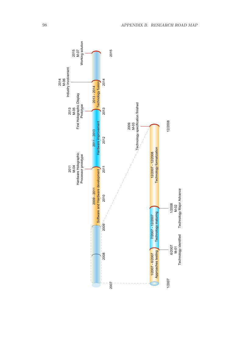
98 APPENDIX B. RESEARCH ROAD MAP
20
07
20
15
20
08
20
09
20
10
20
11
20
12
20
13
20
14
1/2
00
71
2/2
00
8
20
15
M-0
7
Wo
rkin
g s
olu
tio
n
1/2
00
7-
6/2
00
7
Ap
pro
ach
es t
estin
g
20
13
-2
01
4
Te
ch
no
log
y fu
sio
n
7/2
00
7-
12
/20
07
Te
ch
no
log
y m
atu
rin
g
6/2
00
7
M-0
1
Te
ch
no
log
y ide
ntifie
d
20
11
-2
01
3
Ha
rdw
are
im
pro
ve
me
nt
12
/20
07
-1
2/2
00
8
Te
ch
no
log
y fo
rma
liza
tio
n
1/2
00
8
M-0
2
Te
ch
no
log
y M
ajo
r A
dva
nce
20
14
M-0
6
Ind
ustr
y in
vo
lve
me
nt
20
13
M-0
5
Fir
st H
olo
gra
ph
ic D
isp
lay
Pro
toty
pe
20
11
M-0
4
Ha
rdw
are
Ho
log
rap
hic
Pro
ce
sso
r p
roto
typ
e
20
09
M-0
3
Te
ch
no
log
y s
pe
cific
atio
nfin
ish
ed
20
09
-2
01
1
So
ftw
are
an
d H
ard
wa
re d
eve
lop
me
nt

List of Symbols
and Abbreviations
Abbreviation Description Definition
HPO horizontal parallax only page 87SLM spatial light modulator page 39CCD coupled charge detector page 71FFT fast fourier transform page 24GPU graphics processing unit page 39STAR state of the art page 81MIT massachusetts institute of technology page 65CGI computer graphics imagery page 43LCD liquid crystal display page 3CRT cathode ray tube page 3CAD computer aided design page 3LASER light amplification by stimulated emission of radi-
ationpage 7
99

List of Figures
2.1 Illustration of interference . . . . . . . . . . . . . . . . . . . . . . . . . 112.2 A configuration for exploring the coherence [Har96]. . . . . . . . . . . 122.3 Relation between spherical and planar wave [Kra04]. . . . . . . . . . . 162.4 Huygens principle . . . . . . . . . . . . . . . . . . . . . . . . . . . . . 172.5 Kirchhoff formulation of diffraction by a plane screen. [Goo05] . . . . 192.6 Configuration of the Fresnel/Fraunhofer approximation [Goo05]. . . . 232.7 Fresnel approximation for tilted plane . . . . . . . . . . . . . . . . . . 252.8 Intensity of thin cosine amplitude grating. . . . . . . . . . . . . . . . . 262.9 Diffraction grating and diffraction condition. . . . . . . . . . . . . . . 272.10 Plane waves distribution obtained by Fourier transform. . . . . . . . . 292.11 Difference between hologram and photo . . . . . . . . . . . . . . . . . 312.12 Elemental principle of holography. . . . . . . . . . . . . . . . . . . . . 312.13 Inline hologram configuration . . . . . . . . . . . . . . . . . . . . . . . 322.14 Off-axis hologram setup . . . . . . . . . . . . . . . . . . . . . . . . . . 34
3.1 Inline holograms of point radiators . . . . . . . . . . . . . . . . . . . . 463.2 Two modes of ray the casting based approach operation. . . . . . . . . 483.3 Scene composition for FFT synthesis . . . . . . . . . . . . . . . . . . . 513.4 Situation for diffraction evaluation between tilted planes. . . . . . . . 533.5 Scene projection from angles θ and ϕ [AR03]. . . . . . . . . . . . . . . 563.6 Equivalent optical system for the synthesis. [AR03] . . . . . . . . . . . 573.7 Orthogonal projection and sectional plane. . . . . . . . . . . . . . . . 583.8 Paraboloid of revolution. . . . . . . . . . . . . . . . . . . . . . . . . . . 593.9 Sectional coefficients extraction. . . . . . . . . . . . . . . . . . . . . . 593.10 Point source complex texture . . . . . . . . . . . . . . . . . . . . . . . 613.11 Line source complex texture . . . . . . . . . . . . . . . . . . . . . . . . 623.12 Complex texture for a triangle . . . . . . . . . . . . . . . . . . . . . . 633.13 Hogel vector generation according to the imaged points positions. . . . 673.14 Set of 8 basis fringes and their spectrum. [Luc94] . . . . . . . . . . . . 68
100

101
3.15 Occlusion interval determination [Und97]. . . . . . . . . . . . . . . . . 70
4.1 Integration domain of a single sample of an HPO hologram. . . . . . . 744.2 Geometry slicing. . . . . . . . . . . . . . . . . . . . . . . . . . . . . . . 754.3 Modified triangle scanline slicing. . . . . . . . . . . . . . . . . . . . . . 754.4 Principle of visibility check. . . . . . . . . . . . . . . . . . . . . . . . . 774.5 Candidate lines determination. . . . . . . . . . . . . . . . . . . . . . . 774.6 Aligning of the Z-depth. . . . . . . . . . . . . . . . . . . . . . . . . . . 794.7 Angular sampling of the slice geometry. . . . . . . . . . . . . . . . . . 794.8 Distance evaluation. . . . . . . . . . . . . . . . . . . . . . . . . . . . . 80

List of Tables
A.1 Synthesis methods evaluation . . . . . . . . . . . . . . . . . . . . . . . 96
102

List of Algorithms
3.1 Spherical waves based hologram synthesis method. . . . . . . . . . . 453.2 Ray casting method for synthesis with occlusion test. . . . . . . . . 483.3 Reversed mode of ray casting method for synthesis. . . . . . . . . . 493.4 Fresnel approximation based synthesis method. . . . . . . . . . . . . 523.5 Angular spectrum propagation based synthesis method. . . . . . . . 523.6 Synthesis exploiting propagation between tilted planes. . . . . . . . 553.7 Multiple projections based method for Fourier hologram synthesis. . 563.8 Sectional planes based synthesis. . . . . . . . . . . . . . . . . . . . . 593.9 Point diffraction footprint based method. . . . . . . . . . . . . . . . 623.10 Triangle diffraction footprint based method. . . . . . . . . . . . . . 643.11 Diffraction table based hogel vector generation. . . . . . . . . . . . . 68
103

Index
amplitude, 9
angular spectrum, 28
angular speed, 9
approximation
Fraunhofer, 24
Fresnel, 23
bi-polar intensity, 12
coherence, 12
area, 15
length, 14
partial, 13
spatial, 14
temporal, 14
time, 14
complex amplitude, 9
condition
boundary, Kirchhoff, 18
cosine grating, 26
cross-correlation, 13
curl operator, 8
degree of coherence, 12
diffraction, 8, 16
Kirchhoff, 18
Sommerfeld-Rayleigh, 20
diffraction condition, 26
diffraction efficiency, 27
diffraction formula
Fresnel-Kirchhoff, 19
Rayleigh-Sommerfeld, 20
diffraction integral
Fresnel, 24
diffraction model, 8
diffraction order, 26
diffraction pattern, 9
disturbance
electromagnetic, 9
divergence operator, 8
electric field, 8
electromagnetic wave, 8
far field, 24
Fourier hologram, 36
Fraunhofer hologram, 38
Fraunhofer region, 24
Fresnel region, 23
fringe pattern, 10
fringes, 12
Helmholtz equation, 10
hogel, 66
hologram
inline, 32
off-axis, 7
offaxis, 34
holography, 7
digital, 7
optical, 7, 30
Huygens principle, 16
Huygens-Fresnel principle, 16
Image hologram, 37
interference, 8, 10
constructive, 11
destructive, 11
interference pattern, 10, 12
laser, 7
light, 8
coherent, 11
incoherent, 11
infrared, 8
ultraviolet, 8
visible, 8
105
106 INDEX
magnetic field, 8
Maxwell equations, 8
near field, 23
object beam, 8
optical intensity, 10
permeability, 8
permittivity, 8
phase, 9
ray optics, 10
real image, 33
scalar field, 9
scalar wave theory, 9
spatial light modulator, 39
theorem
Green’s, 18
integral, of Helmholtz and Kirchhoff,
18
virtual image, 33
Wave
evanescent, 28
wave
paraboloidal, 16
planar, 10, 15
spherical, 10, 15
wave optics, 7, 8
wave propagation, 21
wavefront, 10, 16, 21
wavefunction, 9
wavelength, 9
wavenumber, 10, 15
wavevector, 15
zero order, 26