diffusion processes in a migrating interface: the thick-interface model

Available online at www.sciencedirect.com

www.elsevier.com/locate/actamat

Acta Materialia 59 (2011) 4775–4786

Diffusion processes in a migrating interface: The thick-interface model

J. Svoboda a, E. Gamsjager b, F.D. Fischer b,⇑, Y. Liu b, E. Kozeschnik c

a Institute of Physics of Materials, Academy of Sciences of the Czech Republic, Zizkova 22, CZ-616 62 Brno, Czech Republicb Institute of Mechanics, Montanuniversitat Leoben, Franz-Josef-Str. 18, A-8700 Leoben, Austria

c Department of Material Science and Technology, ViennaUniversity of Technology, Favoritenstr. 9, A-1040 Vienna, Austria

Received 3 August 2010; received in revised form 4 April 2011; accepted 10 April 2011Available online 9 May 2011

Abstract

During a solid/solid diffusive phase transformation from a parent b-phase to a product a-phase, dissipative processes due to diffusionin the bulk phases as well as rearrangement of the crystal lattice and diffusion in the interfacial region occur. A model has been developedthat accounts for all the above-mentioned dissipative processes. By means of this thick-interface model it is possible to assign a finitethickness and a finite mobility to the interface. The evolution of the mole fraction profiles of the components in the bulk phases andin the interface can be simulated from a given initial state until a steady state or equilibrium is attained. Based on this theoretical frame-work the kinetics of the c/a phase transformation in the Fe-rich Fe–Cr–Ni system is simulated. Starting from a certain initial compo-sition the transformation kinetics exhibits the features of a massive or a bulk diffusion controlled transformation depending ontemperature.� 2011 Acta Materialia Inc. Published by Elsevier Ltd. All rights reserved.

Keywords: Modeling; Phase transformation; Diffusion; Interface migration; Thermodynamic extremal principle

1. Introduction and motivation

Rearrangement of atoms in the migrating interface, sol-ute drag, trans-interface diffusion and spike formation arephenomena occurring to a smaller or larger extent in theinterface and its nearest surroundings during diffusiveand massive transformations. Several models of the inter-face were developed and have been used to describe thetransformation kinetics. The task to model the kinetics ofdiffusive phase transformations becomes less complicated,if the dissipation of some of the above-mentioned processesis negligibly small compared to the remaining processesand can be neglected. Frequently it is assumed that thebulk phases are separated by an infinitely thin, i.e. sharp,interface. Diffusion processes in the interfacial region arethen automatically out of the scope of these sharp interfacemodels.

1359-6454/$36.00 � 2011 Acta Materialia Inc. Published by Elsevier Ltd. All

doi:10.1016/j.actamat.2011.04.020

⇑ Corresponding author.E-mail address: [email protected] (F.D. Fischer).

The simplest sharp interface model is used in the stan-dard package DICTRA [1]. It is assumed that the transfor-mation kinetics is controlled by diffusion processes in thebulk only and local equilibrium prevails at the interface.This implies that no Gibbs energy is dissipated due to lat-tice rearrangement. The simplifying assumption is equiva-lent to an infinite mobility of the interface. Such a modelis suitable to describe the kinetics of bulk diffusion con-trolled diffusive phase transformations.

A sharp interface model, which considers the dissipationdue to lattice rearrangement by a finite interface mobility,has been introduced by Svoboda et al. [2]. The evolutionequations for the transformation kinetics are obtained byusing the thermodynamic extremal principle (TEP), andthe transformation kinetics can be simulated by means ofthis model in the full range – from bulk diffusion controlledto massive growth. In the frame of this model jumps at theinterface of the chemical potentials of the interstitial com-ponents are zero and all of the substitutional componentsare equal [3]. It is evident that diffusion processes in theinterface result in different contact conditions at the

rights reserved.

http://dx.doi.org/10.1016/j.actamat.2011.04.020

mailto:[email protected]

http://dx.doi.org/10.1016/j.actamat.2011.04.020

4776 J. Svoboda et al. / Acta Materialia 59 (2011) 4775–4786

interface. As a consequence of these processes the jumps ofthe chemical potentials of the substitutional componentsneed not be equal. This fact has been discussed, e.g. in Hill-ert’s review paper [4] and by Hillert and Rettenmayr [5].

A completely different sharp interface model is pre-sented by Larsson et al. [6], who considered trans-interfacediffusion instead of atomic rearrangement and Kirkendallshift instead of the interface migration.

The trans-interface diffusion, solute drag as well as theatomic rearrangement in the migrating interface are alsoincorporated into the thick-interface model for the phasetransformation by Odqvist et al. [7]. All mentioned pro-cesses are also treated by the thick-interface model forthe phase transformation by Svoboda et al. [8]. This modelwas applied to the simulations of massive transformationin a ternary substitutional system yielding the steady statesolution of the evolution equations. Both models [7,8]seem, however, to be far too complicated for practicalapplications.

From the cited papers it is evident that a robust andeffective treatment of the coupled dissipative processes inthe migrating interface is required. The motivation andgoal of this paper are to present a thick-interface modelfor the phase transformation in substitutional alloysaccounting for the rearrangement of atoms in the migratinginterface, solute drag, trans-interface diffusion and spikeformation. The mole fraction profile in the migrating inter-face is approximated by a parabola and, thus, described bya limited number of variables. The evolution equations forall variables describing the system are derived from theTEP (see Ref. [9]). The model is used for the simulationof phase transformation in the Fe–Cr–Ni system, andresults of simulations are discussed.

2. Model

2.1. State and kinetic variables of the system

Let us assume a one-dimensional (1-D) system of a unitcross-section area composed of two phases (product phasea and parent phase b) separated by a thick interface. Bothphases are represented by substitutional alloys with s com-ponents. The site fraction profile of each component i isapproximated by a profile determined by a limited numberof variables as depicted in Fig. 1. The thick interface and itsnearest surroundings consist of two a-phase regions left tothe interface characterized by their thicknesses Dn�1 andDn, two b-phase regions Dn+1 and Dn+2 right to the inter-face, and the interfacial region of width h. The systemmoves from the right to the left with a velocity v. The cen-tre of the interface coincides with the origin of the spatiallyfixed coordinate system. Moreover we assume that the par-tial molar volumes X of all components are the same, andno sources and sinks for vacancies act in the system (noKirkendall effect). Then the total length of the systemPm

k¼1Dk þ h remains constant. Furthermore, we assumethat the regions, characterized by Dk (k = 1,. . ., n � 1,

n + 2, . . ., m), move with a velocity v from the right tothe left in the case that a transformation from the parentb-phase to the product a-phase occurs. The region Dn+1

shrinks ( _Dnþ1 ¼ �v) and the region Dn grows with the rate_Dn ¼ v. The values of Dk (k = 1, . . ., n � 1, n + 2, . . ., m)and the thickness h of the interface are kept constant aswell as the sum D as

D ¼ Dn þ Dnþ1: ð1ÞThe mole fractions xik, the fluxes jik and the chemical

potentials lik are defined by the two subscripts i

(i = 1, . . ., s) and k (k = 1, . . ., m), indicating the compo-nent and the location, respectively. The chemical composi-tion of the interface is given by the local mole fractions ofxiL � xin, xiC and xiR � xin+1, with a parabolic profile in theinterface. As a closed system is investigated, the fluxes atthe boundaries of the system are zero:

ji0 ¼ 0; jim ¼ 0: ð2ÞFor no sources and sinks for vacancies in the system, the

vacancy fluxes can be neglected at every point in the sys-tem, leading to the constraintXs

i¼1

jik ¼ 0: ð3Þ

2.2. Mass balances

The mole fractions xik are constrained byXs

i¼1

xik ¼ 1 ðk ¼ 1; . . . ;mÞ;Xs

i¼1

xiC ¼ 1; ð4Þ

and thus the total time derivatives are related by

Xs

i¼1

_xik ¼ 0 ðk ¼ 1; . . . ;mÞ;Xs

i¼1

_xiC ¼ 0: ð5Þ

The mass conservation relations hold in the individualregions characterized by Dk as

Dk _xik ¼Xðjik�1� jikÞ for k ¼ 1; . . . ;n� 1;nþ 2; . . . ;m;

Dn _xiL ¼Xðjin�1� jiLÞ; Dnþ1 _xiR ¼XðjiR� jinþ1Þð6Þ

with the total time derivatives _xiL � dxiLdt , _xiC � dxiC

dt and_xiR � dxiR

dt , since the variables xiL, xiC and xiR are consideredto be dependent only on time t (see Fig. 1 for introductionof the variables).

The parabolic mole fraction profile xi(z, t) in the inter-face is expressed as

xi ¼ xiC � xiL � xiRð Þ zhþ 2 xiL � 2xiC þ xiRð Þ z

h

� �2

: ð7Þ

The material time derivative, being the rate of a quantityin a material point fixed to the lattice and moving with thevelocity v from the right to the left, is given by

_xi ¼@xi

@t� v

@xi

@zð8Þ

Fig. 1. Schematic course of the mole fraction profile of component i in the interface and its surroundings, notation of thermodynamic and geometricquantities.

J. Svoboda et al. / Acta Materialia 59 (2011) 4775–4786 4777

and coincides with the total time derivative. The materialtime derivative _xi in the interface then follows with Eqs.(7) and (8) as

_xiðzÞ ¼ _xiL 2zh

� �2

� zh

� �þ _xiC 1� 4

zh

� �2� �

þ _xiR 2zh

� �2

þ zh

� �

þ v 4 �xiL þ 2xiC � xiRð Þ z

h2þ xiL � xiR

h

� �: ð9Þ

The flux in the interface is given by Eqs. (6) and (9) as

jiðzÞ ¼ jiL �1

X

Z z

�h2

_xiðz0Þdz0 ¼ jin�1 �Dn _xiL

X

� 1

X_xiL

5h24� z2

2hþ 2z3

3h2

� ��

þ _xiR �h

24þ z2

2hþ 2z3

3h2

� �þ _xiC

h3þ z� 4z3

3h2

� �

þ v 2 �xiL þ 2xiC � xiRð Þ z2

h2� 1

4

� ��

þ xiL � xiRð Þ zhþ 1

2

� ��: ð10Þ

Then the fluxes in the position z = 0 and z = h/2 (seeFig. 1) are given by

jiC ¼ jð0Þ ¼ jin�1 �Dn _xiL

X� 1

X_xiL

5h24þ _xiC

h3

�

� _xiRh

24þ vðxiL � xiCÞ

�; ð11Þ

jiR ¼ jh2

� �¼ jin�1 �

Dn _xiL

X� 1

X_xiL

h6þ _xiC

2h3þ _xiR

h6

�

þvðxiL � xiRÞ�: ð12Þ

The value of jin+1 is given by Eqs. (6)3 and (12).Thekinetics of the system can be described by the values ofindependent kinetic variables represented by the fluxes jik(i = 1, . . ., s � 1, k = 1, . . ., n � 1, n + 2, . . ., m � 1), by

the rates of the mole fractions _xiL, _xiC, _xiR

(i = 1, . . ., s � 1) and by the interface velocity v. The valuesof all other kinetic quantities can be obtained from Eqs.(2), (3), (5), and (6).

The TEP can be applied in a straightforward way toobtain the values of the kinetic variables. For the applica-tion of the principle it is necessary to express the rate _G ofthe total Gibbs energy G and the total dissipation Q in thesystem as functions of state variables and of independentkinetic variables and their rates, respectively. The actualvalues of state variables are given by initial conditions ofxik (k = 1, . . ., m) and xiC (i = 1, . . ., s) and by their integra-tion in time by using Eqs. (6). The chemical potentials lik

(k = 1, . . ., m), liL � lin, liC and liR � lin+1 (i = 1, . . ., s)are given functions of xik (k = 1, . . ., m), xiC

(i = 1, . . ., s - 1) and of the temperature T and are consid-ered to be known.

The part of the system containing the interface and itssurroundings is of special concern. The fluxes jin�1 in thea-phase, the rates of the mole fractions, _xiL; _xiC and _xiR,(i = 1, . . ., s � 1) and the interface velocity v can be chosenas the independent kinetic variables of this subsystem.Thus 4s � 3 kinetic variables describe the kinetics of theinterface and its nearest surroundings. The values of thesekinetic variables are provided by an interface moduledescribed later.

2.3. Rate of Gibbs energy

The Gibbs energy G of the system can be calculated as

G ¼ 1

X

Xs

i¼1

Z zR

zL

xili dz

¼ 1

X

Xs

i¼1

Xm

k¼1

Dkxiklik þXs

i¼1

Z h=2

�h=2

xili dz

!

¼ 1

X

Xs

i¼1

Xm

k¼1

Dkxiklik þh6

Xs

i¼1

xiLliL þ 4xiCliC þ xiRliRð Þ" #

;

ð13Þ


if Simpson’s rule is used for the calculation of the integralcorresponding to the interface. The rate _G of the Gibbs en-ergy can be calculated by

_G ¼ 1

X

Xs

i¼1

Xm

k¼1

_Dkxiklik þXs

i¼1

Xm

k¼1

Dk _xiklik

"

þ h6

Xs

i¼1

_xiLliL þ 4 _xiCliC þ _xiRliRð Þ#: ð14Þ

Terms with rates of the chemical potentials vanish dueto the Gibbs–Duhem equation, and only the thicknessesDn and Dn+1 change with time as described above. By usingEqs. (6) and (14) _G can be written as

_G ¼Xs

i¼1

vXðxiLliL � xiRliRÞ þ

Xs�1

i¼1

Xn�1

k¼1

ðjik�1 � jikÞðlik � lskÞ"

þ ðjin�1 � jiLÞðliL � lsLÞ� þXs�1

i¼1

ðjiR � jinþ1Þ linþ1 � lsnþ1

��

þXm

k¼nþ2

ðjik�1 � jikÞðlik � lskÞ#þ h

6X

Xs�1

i¼1

_xiLðliL � lsLÞ½

þ 4 _xiCðliC � lsCÞ þ _xiRðliR � lsR�: ð15Þ

Eq. (15) expresses _G as a linear form of the independentkinetic variables of the system.

2.4. Total Gibbs energy dissipation in the system

The Gibbs energy dissipation Qk in region k

(k = 1, . . ., n � 1, n + 2, . . ., m) is given by

Qk ¼Xs

i¼1

RTXDixik

ZDk

j2ðzÞdz �Xs

i¼1

RTXDk

2Dixikj2

ik�1 þ j2ik

�

¼Xs�1

i¼1

RTXDk

2Dixikj2

ik�1 þ j2ik

�

þ RT XDk

2Dsxsk

Xs�1

i¼1

jik�1

!2

þXs�1

i¼1

jik

!224

35; ð16Þ

if Eq. (2) and the trapezoidal integration rule are used. Thequantity Di denotes the bulk diffusion coefficient of compo-nent i in the a-phase, Da

i , for k = 1, . . ., n � 1, or in the b-phase, Db

i , for k = n + 2, . . ., m. The trapezoidal integra-tion rule works nearly exactly for not too different valuesof jik�1 and jik (which is usually the case). Some inaccuracycan be expected at the ends of the system due to the validityof conditions (2). The application of, in this case exact,Simpson’s rule would, however, lead to a much more com-plicated solution procedure for the fluxes jik (see later theanalytical solution given by Eqs. (27) and (28)).

Similarly one can write the Gibbs energy dissipation Qn

and Qn+1 in regions n and n + 1 following as

Qn�Xs�1

i¼1

RT XDn

2Dai xiL

j2in�1þ j2

iL

�þRT XDn

2Das xsL

Xs�1

i¼1

jin�1

!2

þXs�1

i¼1

jiL

!224

35;

ð17Þ

Qnþ1 �Xs�1

i¼1

RT XDnþ1

2Dbi xiR

j2inþ1 þ j2

iR

�

þ RTXDnþ1

2Dbs xiR

Xs�1

i¼1

jinþ1

!2

þXs�1

i¼1

jiR

!224

35: ð18Þ

If we assume that the diffusion coefficient changes grad-ually from the value Da

i at the left end of the interface overthe value DI

i in the centre of the interface to the value Dbi at

the right end of the interface, then the Gibbs energy dissi-pation Qif in the interface can be calculated by applyingSimpson’s rule as

Qif ¼RT Xh

6

Xs�1

i¼1

ðjiLÞ2

Dai xiLþ 4ðjiCÞ

2

DIi xiCþ ðjiRÞ

2

Dbi xiR

" #

þ RTXh6

Ps�1i¼1 jiL

� �2

Das xsL

þ4Ps�1

i¼1 jiC

� �2

DIsxsC

þPs�1

i¼1 jiR

� �2

Dbs xsR

264

375:ð19Þ

The total dissipation in the system is given by

Q ¼Xm

k¼1

Qk þ Qif þv2

Mð20Þ

with M being the interface mobility.The corresponding expressions for jiL, jiC and jiR, given

by Eqs. (6), (11), and (12), must be inserted into Eqs.(16)–(20). Then the total dissipation in the system Q

becomes a positive definite quadratic form of the indepen-dent kinetic variables.

3. Evolution equations and their solution

3.1. General evolution equations

Let us denote by _ql (l = 1, . . ., m(s � 1) + 1) all indepen-dent kinetic variables being the fluxes jik (i = 1, . . ., s � 1,k = 1, . . ., n � 1, n + 2, . . ., m � 1), the rates of the molefractions _xiL, _xiC, _xiR (i = 1, . . ., s � 1) and the interfacevelocity v. Then the rate _G of the total Gibbs energy repre-sents a linear form in _ql and the total Gibbs energy dissipa-tion Q a quadratic, positive definite form in _ql. The TEPprovides the evolution equations for the independentkinetic variables [9] as

1

2

@Q@ _ql¼ � @

_G@ _ql

; ðl ¼ 1; . . . ;mðs� 1Þ þ 1Þ ð21Þ

being a set of linear equations for _ql. The set of Eqs. (21)can be rewritten as

Xmðs�1Þþ1

k¼1

Akl _qk ¼ F l; ðl ¼ 1; . . . ;mðs� 1Þ þ 1Þ ð22Þ

with the coefficients

Akl ¼1

2

@2Q@ _qk@ _ql

ð23Þ


and the right side

F l ¼ �@ _G@ _ql

: ð24Þ

The quantities Akl and Fl are independent of _ql

(l = 1, . . ., m(s � 1) + 1) and can easily be produced bymathematics processors as MAPLE 8 (http://www.scien-tific.de/maple.html).

As the actual state of the system is given by the statevariables, represented by the values of xik, (i = 1, . . .,s � 1, k = 1, . . ., m), xiL, xiC, xiR (i = 1, . . ., s � 1) and bythe values of Dk, (k = 1, . . ., m), the rates of the state vari-ables coincide either with the kinetic variables _ql or they arerelated by Eqs. (6) and (12) and by

_Dn ¼ v; _Dnþ1 ¼ �v;_Dk ¼ 0 ðk ¼ 1; . . . ; n� 1; nþ 2; . . . ;mÞ: ð25Þ

It should be noted that the state variables evolve in such away that the total amount of moles Ni of all components i,(i = 1, . . ., s � 1) remains constant, i.e.

1

X

Xm

k¼1

Dkxik þh6

xiL þ 4xiC þ xiRð Þ !

¼ N i ¼ const:; ð26Þ

in accordance with the assumption of a closed system.

3.2. Solution of evolution equations

A subset of the kinetic variables, namely jik(i = 1, . . ., s � 1, k = 1, . . ., n � 2, n + 2, . . ., m � 1), canbe determined analytically in the same way as presentedin Ref. [2], resulting in

jik ¼ �Bik likþ1 � lik �Ps

l¼1Blk llkþ1 � llk

�Psl¼1Blk

� �ð27Þ

with

Bik ¼2

RT X Dkxik Dikþ Dkþ1

xikþ1Dikþ1

� � : ð28Þ

Then the set of Eqs. (22) reduces to a subset of linearequations of dimension 4s � 3 for jin�1, _xiL, _xiC, _xiR,(i = 1, . . ., s � 1) and v. The respective coefficients as sub-sets of Akl and Fl are calculated by applying MAPLE 8(http://www.scientific.de/maple.html) and exported into aFORTRAN code. The system of linear equations for thekinetic variables jin�1, _xiL, _xiC, _xiR, (i = 1, . . ., s � 1) and v

is solved numerically. This procedure represents the inter-face module mentioned at the end of Section 2.3. The mod-ule takes Dn�1, Dn, Dn+1, Dn+2, xin�1, xin+2, xiL, xiC and xiR

(i = 1, . . ., s � 1), the diffusion coefficientsDa

i ;DIi ;D

bi ; ði ¼ 1; . . . ; sÞ and the interface mobility M as

input quantities and provides the values of the kinetic vari-ables jin�1, _xiL, _xiC, _xiR, (i = 1, . . ., s � 1) and v as outputquantities.

To ensure a sufficient accuracy of simulations a densemesh near the interface must be chosen. As the interface

moves relatively to the nodal points, this fact provokes afrequent elimination or addition of nodes right and leftto the interface and may cause numerical instability. Thus,similarly as in Ref. [2], it is advantageous to keep the posi-tions of the nodal points fixed. Therefore, we switch frommoving nodal points to fixed nodal points and, thus, therates of quantities at these points are described by partialtime derivatives. The only exceptions are the nodal pointsat the ends of the system, which must remain moving. Thenit holds that

@Dk

@t¼ 0; ðk ¼ 2; . . . ;m� 1Þ; @D1

@t¼ v and

@Dm

@t¼ �v;

ð29Þand only the nodal points immediate to the ends must beadded or eliminated if D1 gets too large or Dm gets toosmall.

For a continuous profile of the mole fractions the partialtime derivatives can be calculated from the material timederivatives by means of formula (8) as

@xi

@t¼ _xi þ v

@xi

@z: ð30Þ

In a discrete description, using a net of non-equidistantnodal points, however, the partial derivatives must be cal-culated numerically. This doing may cause inaccuracies sothat the total amounts of moles Ni from Eq. (26) are notconserved. To guarantee the conservation, we recommendusing the following set of relations valid for a general dis-cretization, which turns into Eq. (30) for infinitesimally finediscretization:

v > 0 :@xik

@t¼ _xik þ v

xikþ1 � xik

Dk;

ði ¼ 1; . . . ; s; k ¼ 1; . . . ; n� 1; nþ 2; . . . ;m� 1Þ; ð31Þ@xin

@t¼ _xin; ði ¼ 1; . . . ; sÞ; ð32Þ

@xinþ1

@t¼ _xinþ1 þ v

xinþ2 � xinþ1

Dnþ1 þ h=6; ði ¼ 1; . . . ; sÞ; ð33Þ

@xim

@t¼ _xim; ði ¼ 1; . . . ; sÞ; ð34Þ

v < 0 :@xi1

@t¼ _xi1; ði ¼ 1; . . . ; sÞ; ð35Þ

@xik

@t¼ _xik þ v

xik � xik�1

Dk;

ði ¼ 1; . . . ; s; k ¼ 2; . . . ; n� 1; nþ 2; . . . ;mÞ; ð36Þ@xin

@t¼ _xin þ v

xin � xin�1

Dn þ h=6; ði ¼ 1; . . . ; sÞ; ð37Þ

@xinþ1

@t¼ _xinþ1; ði ¼ 1; . . . ; sÞ: ð38Þ

The h/6 term in Eqs. (33) and (37) stems from the applica-tion of Simpson’s rule in Eq. (26).

The following check can be performed. The materialtime derivative of Eq. (26) in the original net of movingnodal points is given by

http://www.scientific.de/maple.html



Fig. 2. Phase boundaries between the a-single phase region and the(a + c) region for certain temperatures. The initial composition is markedby a circle.


vðxin � xinþ1Þ þXn�1

k¼1

Dk _xik þXm�1

k¼nþ2

Dk _xik þ Dn _xin þ Dnþ1 _xinþ1

þ Dm _xm þh6ð _xin þ 4 _xiC þ _xinþ1Þ ¼ 0: ð39Þ

The partial time derivatives of Eq. (26) reads afterswitching to fixed nodal points as

vðxi1 � ximÞ þXn�1

k¼1

Dk@xik

@tþXm�1

k¼nþ2

Dk@xik

@tþ Dn

@xin

@t

þ Dnþ1

@xinþ1

@tþ Dm

@xm

@tþ h

6

@xin

@tþ 4

@xiC

@tþ @xinþ1

@t

� �¼ 0:

ð40Þ

Now one can easily show that the insertion of Eqs. (31)–(38) into Eq. (40) yields Eq. (39), which proves the massconservation for switching to fixed nodal points.

4. Results of simulations and their discussion

By means of the derived evolution equations the kineticsof the c to a transformation in the Fe-rich Fe–Cr–Ni sys-tem is simulated. The length of the system is set to0.5 lm. The thickness of the interface is generally consid-ered to be one or two interatomic distances and thush = 0.3 nm is chosen. The molar volume is given byX = 7.3 � 10�6 m3 mol�1 and assumed to be independentof chemical composition and phase. The initial chemicalcomposition is set to xCr = 0.01 and xNi = 0.015 in bothphases. Simulations are performed for temperatures,T = 1055 K, 1060 K, 1061 K, 1062 K, 1065 K and1080 K. The chemical potentials li are calculated accordingto the thermodynamic assessments [10–12]. Similar to thework presented in Ref. [8] we assume that the thermody-namic properties in the centre of the interface (see Fig. 1,z = 0) can be approximated by the thermodynamic proper-ties of the liquid phase, however, extrapolated to its valuecorresponding to the temperature used in the calculations.Usually incoherent interfaces at high temperature areassumed as thin layers of amorphous structure, and theundercooled liquid seems to be a good approximation ofsuch structure. The chemical potentials in the a-phaseand in the c-phases as well as in the interface are weightedby cubic Hermite interpolation splines [8]. The diffusioncoefficients in the interface are also interpolated by Hermitepolynomials as described in Ref. [8].

The relevant part of the phase diagram is the Fe-richcorner in the Fe–Cr–Ni system, where the c/a phase trans-formation occurs. The a/(a + c) phase boundaries are com-puted by minimizing the Gibbs energy of the system andare depicted in Fig. 2 for all chosen temperatures. The c/a transformation occurs for the temperatures 1055 K and1060 K in the a-single-phase region and for higher temper-atures the transformation occurs in the (a + c)-two phaseregion.

The values of the thermally activated diffusion coeffi-cients of the components in the product a-phase, in theinterface and in the parent c-phase and the value of thethermally activated interface mobility M, are specified inTable 1. For the interface mobility M the value of Krielaart[15] is chosen, which is approximately 500 times below thevalue estimated in pure Fe in Ref. [16].

As the solubility of Ni and Cr in the interface region isconsiderably higher than in the a and c bulk phases for alltemperatures investigated, Ni and Cr atoms segregate atthe interface and are dragged during the phase transfor-mation. The typical steady state mole fraction profiles inthe interface and its nearest surroundings, correspondingto a massive transformation [17], are observed atT = 1055 K. The mole fraction profiles of Ni at differenttimes are plotted in Fig. 3a, and it can be concluded thatthe interface migrates with a constant velocity. The molefraction peaks, indicating the position of the interface,move equal distances from the left to the right for equaltime periods. It is not possible to get an idea about thesegregation profiles in the interface from Fig. 3a as theinterface is thin compared to the shown spatial rangeand the maximum segregation level exceeds the plottedxNi range. However, a closer view to the evolution ofthe mole fractions in the interface and its nearest sur-roundings can be provided, if the profiles for differentinstants are shifted so that the centre of the interfacealways coincides.

The deviation from the initial composition around z = 0in Fig. 3a follows from the mass balance. The Ni spike andthe Cr spike evolve in the interface and thus Ni and Cr dif-fuse from the a-phase into the interface. During the trans-formation the deviation from the initial composition in thea-phase decreases gradually. By this deviation from the ini-tial composition during the initial stages of the phase trans-formation it is demonstrated that we do not start from asteady state profile, but we let the profile evolve until steadystate or equilibrium is attained.

Table 1Diffusion coefficients in the Fe–Cr–Ni system and grain boundarydiffusivity as an approximation for the diffusivity in the interface andthe interface mobility. QA is the activation energy.

Diffusion coefficient D0 (m2 s�1) QA (J mol�1) Ref.

Cr in a phase 3.2 � 10�4 2.4 � 105 [13]Ni in a phase 4.8 � 10�5 2.4 � 105 [13]Fe in a phase 1.6 � 10�4 2.4 � 105 [13]Cr in interface 2.2 � 10�4 1.55 � 105 [14]Ni in interface 0.22 � 10�4 1.55 � 105 [14]Fe in interphase 1.1 � 10�4 1.55 � 105 [14]Cr in c phase 3.5 � 10�4 2.86 � 105 [13]Ni in c phase 3.5 � 10�5 2.86 � 105 [13]Fe in c phase 7 � 10�5 2.86 � 105 [13]Interface mobility M0 (m2 s kg�1) QA (J mol�1)Interface 4.1 � 10�7 1.4 � 105 [15]

Fig. 3. Mole fraction profiles for different instants at T = 1055 K. Thinvertical lines indicate the position of the interface. Mole fraction spikes inthe parent phase in front of the migrating interface are highlighted in grey.(a) Profiles of the Ni-mole fraction in the whole system. (b) Profiles of theNi-mole fraction in the interface and its vicinity. (c) Profiles of the Cr-molefraction in the interface and its vicinity.


The Ni profiles are presented in Fig. 3b. The shape ofthe profile does not change with time, and an extremelythin spike (highlighted in grey) is observed in the parentphase. The Cr profiles are shown in Fig. 3c. Compared tothe Ni profiles, the Cr spike in the parent phase is lowerand its half width is larger due to a higher diffusivity ofCr in the c-phase. Of course, one could argue that it hasno sense to talk about spike thicknesses of the order ofmagnitude of 1/100 of an interatomic distance. However,if one assumes the 1-D case and makes a statistics from asufficiently large area of the interface, corresponding to asufficiently large number of atoms in the spike, then thereasoning makes sense.

A detailed analysis of the transformation was performedfor T = 1060 K, i.e. for a temperature for which the initialcomposition almost coincides with the a/(a + c) phaseboundary, as can be seen in Fig. 2. In this exceptional casethe total length of the system is increased to 2 lm, so thatthe interface velocity can be stabilized. In Fig. 4 the molefraction profiles of Ni are plotted in the same way as inFig. 3b. One can clearly observe that the profile approachesa steady state. However, the system requires a transitiontime period from the start of the transformation to thesteady state being orders of magnitude higher atT = 1060 K compared to T = 1055 K. The profiles att = 1000 s (solid circles) and at t = 2000 s (solid line) can-not be distinguished from each other, indicating that steadystate is reached.

In this context the difference between the seminal workby Cahn [18] and the present model should be expressed.Cahn assumes in his model that the profile of the chemicalpotential of the dragged component in the interface, thediffusion coefficient of the dragged component andthe velocity of migration are known. Then Cahn solvedthe steady-state diffusion equation in the migrating inter-face for zero diffusive flux at the contact of the productphase with the interface, obtained the concentration profileof the dragged component and calculated the total dragforce. The resulting interface velocity followed then fromthe balance equation of forces acting at the interface. This

equation is an implicit equation for the interface velocity,which can be resolved analytically only for special cases.

In our model we also assume that the chemical potentialof the dragged component in the interface and the diffusioncoefficient of the dragged component are known. We,however, expect a parabolic concentration profile in the

Fig. 4. Mole fraction profiles of Ni for different instants at T = 1060 K.The thin vertical lines indicate the position of the interface.

Fig. 5. Mole fraction profiles of Ni for different instants at T = 1061 K.Thin vertical lines indicate the position of the interface. (a) Profiles of theNi-mole fraction in the whole system. (b) Profiles of the Ni-mole fractionin the interface and its vicinity.


interface (the height of the parabola is given by its value inthe centre of the interface) and allow the diffusive interac-tion of the interface with both adjacent crystals (our solu-tion is not limited to zero diffusive flux at the contact of theproduct phase with the interface). We start with a certain

profile of the dragged component in the system. The rateof change of the profile and the actual interface velocityare determined from TEP. Thus, no implicit equation forthe interface velocity must be solved. Under steady-stateconditions, corresponding to the massive transformation,the concentration profile and the interface velocityapproach very quickly their stationary values.

The features of the transformation kinetics are alsostudied at T = 1061 K. The composition lies already inthe two-phase region at this temperature. The mole frac-tion profiles at different instants are plotted in Fig. 5a.The characteristics of the transformation seem to be thatof a massive transformation. However, the Ni-mole frac-tion in the product phase is slightly different to the Ni-molefraction in the parent phase far from the interface. This is aclear difference to the result observed at T = 1055 K (seeFig. 3a), where these mole fractions do not deviate fromeach other provided that the boundary of the system is suf-ficiently far away. A closer view at the profiles in the inter-face and its vicinity exhibits also some slight deviationsfrom the character of a massive transformation (seeFig. 5b) as the half thickness of the spike graduallyincreases.

At 1065 K the mentioned effects are further increasedcompared to 1061 K, see Fig. 6. Finally, it can be statedthat the transition from the massive transformation to adiffusion transformation occurs in a continuous mannerwith increasing transformation temperature.

Finally, the transformation kinetics is simulated for atemperature T = 1080 K, see Fig. 7. The kinetics is evi-dently controlled by bulk diffusion.

The evolution of the interface velocities for differenttemperatures T = 1055 K, 1060 K, 1061 K, 1062 K,1065 K and 1080 K is plotted in Fig. 8. For T = 1055 Kthe interface velocity quickly stabilizes at a certain value(Fig. 8a). A constant interface velocity indicates that thetransformation occurs in the massive mode characterizedby identical chemical compositions in the product a-phasenear the interface (described by xin) and in the parent c-phase (described by xim) far from the interface. The velocitystabilizes more slowly at temperature T = 1060 K (Fig. 8b)compared to 1055 K (Fig. 8a), but a steady state is finallyreached and the transformation can be considered as amassive one. For T = 1061 K, 1062 K and 1065 K theinterface velocity, depicted in Fig. 8c, decreases monoto-nously and eventually goes to zero when equilibrium isreached. This is the case for T = 1080 K – see Fig. 8d.The velocity plotted vs. t�1/2 demonstrates even clearerwhether a steady state or a constant velocity is attainedafter a certain period of transformation (small t�1/2 values)or if the equilibrium state will eventually be reached(Fig. 8d). Whereas the transformations at 1055 K and1060 K yield to a constant velocity, the interface velocitycorresponding to the transformation in the two-phaseregion (T P 1061K) gradually decreases (Fig. 8e).

Equivalent to the jump [[a]] of a quantity a at the sharpinterface – described by the difference ao � an with the

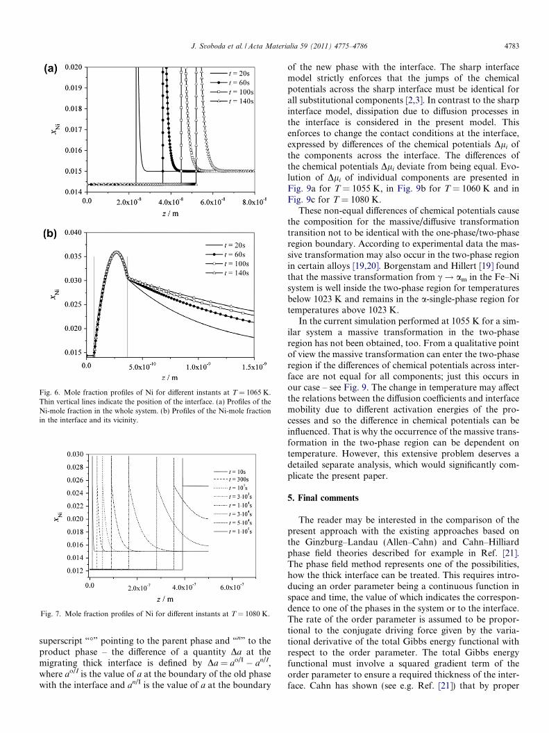
Fig. 6. Mole fraction profiles of Ni for different instants at T = 1065 K.Thin vertical lines indicate the position of the interface. (a) Profiles of theNi-mole fraction in the whole system. (b) Profiles of the Ni-mole fractionin the interface and its vicinity.

Fig. 7. Mole fraction profiles of Ni for different instants at T = 1080 K.


superscript “�” pointing to the parent phase and “n” to theproduct phase – the difference of a quantity Da at themigrating thick interface is defined by Da = ao/I � an/I,where ao/I is the value of a at the boundary of the old phasewith the interface and an/I is the value of a at the boundary

of the new phase with the interface. The sharp interfacemodel strictly enforces that the jumps of the chemicalpotentials across the sharp interface must be identical forall substitutional components [2,3]. In contrast to the sharpinterface model, dissipation due to diffusion processes inthe interface is considered in the present model. Thisenforces to change the contact conditions at the interface,expressed by differences of the chemical potentials Dli ofthe components across the interface. The differences ofthe chemical potentials Dli deviate from being equal. Evo-lution of Dli of individual components are presented inFig. 9a for T = 1055 K, in Fig. 9b for T = 1060 K and inFig. 9c for T = 1080 K.

These non-equal differences of chemical potentials causethe composition for the massive/diffusive transformationtransition not to be identical with the one-phase/two-phaseregion boundary. According to experimental data the mas-sive transformation may also occur in the two-phase regionin certain alloys [19,20]. Borgenstam and Hillert [19] foundthat the massive transformation from c! am in the Fe–Nisystem is well inside the two-phase region for temperaturesbelow 1023 K and remains in the a-single-phase region fortemperatures above 1023 K.

In the current simulation performed at 1055 K for a sim-ilar system a massive transformation in the two-phaseregion has not been obtained, too. From a qualitative pointof view the massive transformation can enter the two-phaseregion if the differences of chemical potentials across inter-face are not equal for all components; just this occurs inour case – see Fig. 9. The change in temperature may affectthe relations between the diffusion coefficients and interfacemobility due to different activation energies of the pro-cesses and so the difference in chemical potentials can beinfluenced. That is why the occurrence of the massive trans-formation in the two-phase region can be dependent ontemperature. However, this extensive problem deserves adetailed separate analysis, which would significantly com-plicate the present paper.

5. Final comments

The reader may be interested in the comparison of thepresent approach with the existing approaches based onthe Ginzburg–Landau (Allen–Cahn) and Cahn–Hilliardphase field theories described for example in Ref. [21].The phase field method represents one of the possibilities,how the thick interface can be treated. This requires intro-ducing an order parameter being a continuous function inspace and time, the value of which indicates the correspon-dence to one of the phases in the system or to the interface.The rate of the order parameter is assumed to be propor-tional to the conjugate driving force given by the varia-tional derivative of the total Gibbs energy functional withrespect to the order parameter. The total Gibbs energyfunctional must involve a squared gradient term of theorder parameter to ensure a required thickness of the inter-face. Cahn has shown (see e.g. Ref. [21]) that by proper

Fig. 8. (a–d): Interface velocity v vs. transformation time t for different temperatures, (e): Interface velocity v vs. 1/(transformation time t)1/2 for differenttemperatures.


choice of the Gibbs energy functional and by proper choiceof the inner product used in the variational derivative ofthe Gibbs energy functional, various already known evolu-tion equations for field variables can be obtained. Thismathematically motivated approach provides a deeperinsight into the understanding of the problem and raiseshopes in general principles for microstructure evolution.

Our approach is based on the application of the thermo-dynamic extremal principle (TEP) originally formulated byOnsager in 1931 [22]. From the view of physics the TEP

represents a strong formulation of the second law of ther-modynamics. The path of the evolution of the system isselected unambiguously as it corresponds to the con-strained maximum of the entropy production rate (dissipa-tion). A general formulation of the TEP was given byZiegler in his book [23], stating that the dissipation hasto be maximized with the constraint that the dissipationmust be identical to the negative rate of Gibbs energy. Thisformulation was adopted and reformulated for discreteparameters by Svoboda et al. in 1991, [24] and later on

Fig. 9. Difference of chemical potentials of Fe, Cr and Ni across theinterface for different temperatures as a function of transformation time.(a) T = 1055 K, (b) T = 1060 K, (c) T = 1080 K.


extended to a generalized tool [9] with applications inseveral areas of micromechanics. Specifically, we refer toa rigorous derivation of the diffusion equations for systemswith non-ideal sources and sinks for vacancies [25,26].

If a system is described by field variables (like concentra-tion profiles), TEP can be used in its variational form (as itwas originally formulated by Onsager) and reproduces theevolution equations for the field variables. Of course, oneof the field variables can be the order parameter (anaccording study is in preparation). Thus, both TEP as well

as the Cahn variational principle (see e.g. Ref. [21]) can beused for the description of system evolution by field vari-ables and provide the complete set of evolution equations.However, there exists at least one substantial differencebetween both principles: Cahn’s extremal principle per-forms variations with respect to state parameters andTEP performs variations with respect to rates of stateparameters or generalized fluxes related to the rates of stateparameters.

In our model of the thick interface an optimized set ofdiscrete parameters instead of field variables is selectedfor the description of the system. The derivation of the evo-lution equations can be performed in a straightforwardway by means of TEP formulated in terms of discreteparameters [9,24]. However, dealing with discrete parame-ters would make it necessary to modify the Cahn varia-tional principle. Our approach allows choosing theinterface thickness as a fixed quantity, and the interfaceitself can be considered as spatially weighted combinationof three phases. No order parameters need to be introducedand consequently its squared gradient term does not enterthe total Gibbs energy. Such an approach allows also char-acterizing the concentration profile in the interface, e.g. bya parabolic shape function, for which compared to thesharp interface approach only one additional parameteris necessary.

The reader might ask why such a complicated solutionprocedure must be followed, if only two processes areinvolved – diffusion of the components and migration ofthe interface with finite mobility – having in mind that thephase field method provides simple equations and a robustmethod for their solution on a fixed equidistant grid.

Let us check the possibility of application of the phasefield method for the problem at hand. We need to workwith a system of total length of at least 10�7 m and timesup to seconds. To obtain a sufficiently accurate concentra-tion spike in front of the migrating interface, the grid dis-tance must be of the order of 10�11 m. Thus, anextremely fine grid with at least 104 nodal points is neces-sary. Furthermore, one must take into account that the dif-fusion coefficient in the interface is several orders ofmagnitude higher than in the bulk. Both these facts causeextreme complications with respect to the stability of thenumerical solution of the diffusion equation for requiredtimes. In addition, the interface mobility must also betaken sufficiently high to ensure an interface migration con-trolled by the diffusion in the interface. Consequently, thekinetic coefficient in the evolution equation for the orderparameter must also be high. All these facts certainlyincrease the complications with stability of the numericalsolution on a very fine grid. To sum up, one cannot expectthat the present problem is solvable by means of the phasefield method with existing computers in reasonable compu-tational times.

The present TEP-based model avoids the problems withthe stability of the numerical solution by several subtlemeasures:


� Solving the diffusion equation in the interface by using aparabolic shape function with one evolving parameter(the height of the profile in the centre of the interface).The concept is open also for a more flexible shape func-tions, e.g. polynomials of fourth order, by introducingmore evolving parameters.� Using a non-equidistant grid with highest density of

nodal points in the location of the concentration spikein front of the migrating interface. There the diffusioncoefficients obtain small values corresponding to thebulk and cause no numerical difficulty.� A grid moving with the interface.� Incorporating the finite mobility of the interface by one

term in the total dissipation. This allows varying themobility within a wide range without loss of stabilityof the numerical solution.

6. Summary

A thick-interface model for solid/solid diffusive phasetransformation is presented. The model accounts for dissi-pative processes due to diffusion in the bulk phases and dueto rearrangement of the crystal lattice and diffusion in theinterfacial region. The mole fraction profiles of all compo-nents are assumed to be parabolic ones in the interface anddescribed by one parameter for each component, i.e. themole fraction in the centre of the interface. The actual stateof the system is described by a certain number of variableswhose evolution equations are derived by application ofthe thermodynamic extremal principle (TEP). The pro-cesses in the thick interface are treated by an interface mod-ule, which implicitly determines the contact conditions atthe migrating interface.

The model is used for extensive simulations of the diffu-sive and massive transformations in the Fe-rich Fe–Cr–Nisystem. Equal jumps of chemical potentials of all substitu-tional components are obtained by sharp interface modelsand, thus the massive transformation analysed in the sharpinterface approach can occur only in the one-phase region.By means of the current, thick-interface model, however,the differences of the chemical potentials of the componentsat the migrating interface can have different values. There-fore, massive transformation in the two-phase region couldbe predicted with this thick-interface model. The gradualchange from a massive to a bulk diffusion controlled phasetransformation depending on composition and tempera-ture is demonstrated.

Acknowledgements

The authors appreciate the funding by Austrian FWFunder the project “Massive Transformation – Experiments

and Simulations”, Project number P20709-N20. J.S.acknowledges also the funding by Ministry of Education,Youth and Sports of the Czech Republic within the COSTMP0701 Project Number OC 10029. Financial support bythe Austrian Federal Government (in particular from theBundesministerium fur Verkehr, Innovation und Technol-ogie and the Bundesministerium fur Wirtschaft und Arbeit)and the Styrian Provincial Government, represented by Os-terreichische Forschungsforderungsgesellschaft mbH andby Steirische Wirtschaftsforderungsgesellschaft mbH, with-in the research activities of the K2 Competence Centre on“Integrated Research in Materials, Processing and ProductEngineering”, operated by the Materials Center LeobenForschung GmbH in the framework of the Austrian CO-MET Competence Centre Programme, is gratefullyacknowledged.

References

[1] Borgenstam A, Engstrom A, Hoglund L, Agren J. J Phase Equilib2000;21:269.

[2] Svoboda J, Gamsjager E, Fischer FD, Fratzl P. Acta Mater 2004;52:959.

[3] Gamsjager E. Philos Mag Lett 2008;88:363.[4] Hillert M. Acta Mater 1999;47:4481.[5] Hillert M, Rettenmayr M. Acta Mater 2003;51:2803.[6] Larsson H, Strandlund H, Hillert M. Acta Mater 2006;54:945.[7] Odqvist J, Sundman B, Agren J. Acta Mater 2003;51:1035.[8] Svoboda J, Vala J, Gamsjager E, Fischer FD. Acta Mater 2006;54:

3953.[9] Svoboda J, Turek I, Fischer FD. Philos Mag 2005;85:3699.

[10] Dinsdale AT. CALPHAD 1991;15:317.[11] Hillert M, Qiu C. Metall Mater Trans A 1991;22A:2187.[12] Hillert M, Qiu C. Metall Mater Trans A 1992;23A:1593.[13] Lee BJ, Oh KH. Z Metallkd 1996;87:195.[14] Fridberg J, Torndahl L-E, Hillert M. Jernkont Ann 1969;153:

263.[15] Krielaart GP, Sietsma J, van der Zwaag S. Mater Sci Eng 1997;A237:

216.[16] Kozeschnik E, Gamsjager E. Metall Mater Trans 2006;37A:

1791.[17] Aaronson HI, Enomoto E, Lee JK. Mechanisms of diffusional phase

transformations in metals and alloys. Boca Raton, FL: CRC Press;2010.

[18] Cahn JW. Acta Mater 1962;10:117.[19] Borgenstam A, Hillert M. Acta Mater 2000;48:2765.[20] Veeraraghavan D, Wang P, Vasudevan VK. Acta Mater 1999;47:

3313.[21] Craig Carter W, Taylor JE, Cahn JW. JOM 1997:30.[22] Onsager L. Phys Rev 1931;37:405.[23] Ziegler H. An introduction to thermodynamics. Amsterdam: North

Holland; 1977 [Section 15.1].[24] Svoboda J, Turek I. Philos Mag 1991;B64:749.[25] Svoboda J, Fischer FD, Fratzl P. Acta Mater 2006;54:3043.[26] Fischer FD, Svoboda J. Acta Mater 2010;58:2698.

diffusion processes in a migrating interface: the thick-interface model

Documents