diffusion in heterogeneous systems studied by laser...
TRANSCRIPT

Diffusion in heterogeneous systems studied by
Laser Scanning Confocal Microscopy and
Fluorescence Correlation Spectroscopy
Dissertation
zur Erlangung des Grades
"Doktor der Naturwissenschaften"
am Fachbereich Chemie, Pharmazie und Geowissenschaften
der Johannes Gutenberg-Universität Mainz
Mikheil Doroshenko
geboren am 31.08.1987
in Tiflis (Georgien)
Mainz – 2013

- 2 -

- 3 -
Dekan: (is given in printed version) 1. Berichterstatter: (is given in printed version)
2. Berichterstatter: (is given in printed version)
Tag der mündlichen Prüfung: (is given in printed version)

- 4 -
Die vorliegende Arbeit wurde im Zeitraum von Oktober 2010 bis
Dezember 2013 am Max‐Planck‐Institut für Polymerforschung, unter der
Betreuung von (is given in printed version) angefertigt.

- 5 -
“Life is not a problem to be solved,
but a reality to be experienced.”
-Søren Kierkegaard

- 6 -

- 7 -
ABSTRACT
Understanding and controlling the mechanism of the diffusion of small
molecules, macromolecules and nanoparticles in heterogeneous environments is of
paramount fundamental and technological importance. The aim of the thesis is to
show, how by studying the tracer diffusion in complex systems, one can obtain
information about the tracer itself, and the system where the tracer is diffusing.
In the first part of my thesis I will introduce the Fluorescence Correlation
Spectroscopy (FCS) which is a powerful tool to investigate the diffusion of
fluorescent species in various environments. By using the main advantage of FCS
namely the very small probing volume (<1µm3) I was able to track the kinetics of
phase separation in polymer blends at late stages by looking on the molecular tracer
diffusion in individual domains of the heterogeneous structure of the blend. The
phase separation process at intermediate stages was monitored with laser scanning
confocal microscopy (LSCM) in real time providing images of droplet coalescence
and growth.
In a further project described in my thesis I will show that even when the
length scale of the heterogeneities becomes smaller than the FCS probing volume
one can still obtain important microscopic information by studying small tracer
diffusion. To do so, I will introduce a system of star shaped polymer solutions and
will demonstrate that the mobility of small molecular tracers on microscopic level is
nearly not affected by the transition of the polymer system to a “glassy” macroscopic
state.
In the last part of the thesis I will introduce and describe a new stimuli
responsive system which I have developed, that combines two levels of
nanoporosity. The system is based on poly-N-isopropylacrylamide (PNIPAM) and
silica inverse opals (iOpals), and allows controlling the diffusion of tracer molecules.

- 8 -
ZUSAMMENFASSUNG
Das Verständnis und die Kontrolle des Diffusionsmechanismus kleiner
Moleküle, Makromoleküle und Nanopartikel in heterogenen Umgebungen ist von
höchst fundamentaler und technologischer Bedeutung. Das Ziel dieser Arbeit ist es
zu zeigen, wie durch die Studie der Diffusion einer Markersubstanz in komplexen
Systemen Informationen über den Marker selbst und das System in dem er
diffundiert erhalten werden können.
Im ersten Teil meiner Arbeit werde ich in die Fluoreszenzkorrelations-
spektroskopie (FCS) einführen, die ein mächstiges Werkzeug zur Untersuchung der
Diffusion fluoreszenter Spezies in verschiedenen Umgebungen ist. Durch die
Ausnutzung des Hauptvorteils der FCS, nämlich dem sehr kleinen
Probenvolumen (<1µm3) war es mir möglich die Kinetik der Phasenseparation in
Polymermischungen in späten Stadien durch die Betrachtung der moleularen
Markerdiffusion in einzelnen Domänen der heterogenen Struktur der Mischung zu
verfolgen. Der Phasenseparataionsprozess in Zwischenstadien wurde mit konfokaler
Laserrastermikroskopie (LSCM) in Echtzeit betrachtet, aufgenommen wurden Bilder
von Tröpfchenkoaleszenz und -wachstum.
In einem weiteren Projekt, das in meiner Arbeit beschrieben wird, werde ich
zeigen dass sogar bei Heterogenitäten von Längenskalen kleiner als das FCS
Probenvolumen immer noch wichtige mikroskopische Informationen durch die
Betrachtung der Diffusion der kleinen Marker erkahlten werden kann. Dafür werde
ich das System eines sternförmigen Polymers einführen und werde zeigen dass die
Mobilität von kleinen molekularen Markern auf mikroskopischer Ebene nahezu nicht
vom Übergang des Polymersystems in einen "glasigen" makroskopischen Zustand
beeinflusst wird.
Im letzten Teil meiner Arbeit werde ich ein neues, stimulussensitives System
einführen und beschreiben, das ich entwickelt habe und das zwei Ebenen von
Nanoporosität vereint. Das System basiert auf Poly-N-isopropylacrylamid
(PNIPAM) und inversen Silicaopalen (iOpals) und erlaubt die Kontrolle der
Diffusion von Markermolekülen.

- 9 -
Table of content
Abstract/ Zusammenfassung…………………………………..………………….. 7
Table of contents ………………………………………….……………………. 9
1. Introduction ……………………………………………………13
1.1. Diffusion ………………………………………………………………..13
1.1.1. Theory of diffusion ………………………………………………14
1.1.1.1. Fick’s first law ………………………………………………14
1.1.1.2. Fick’s second law …………………………………………...17
1.1.2. Random walk theory ……………………………………………..18
1.1.2.1. Simplified model ……………………………………… ……19
1.2. Motivation ………………………………………………………………22
2. Methods …………………………………………………………25
2.1. Confocal Laser Scanning Microscopy …………….……………………25
2.1.1. Operational Principle ……………………………………………25
2.1.2. Resolution …………………………………………..……………28
2.1.3. Laser Illumination and Fluorescence ……………………………29
2.1.4. LSCM setup used in this work ….……………………………….30
2.2. Fluorescence correlation spectroscopy (FCS) ………………………….31
2.2.1. Introduction to FCS ……………………………………………..31
2.2.2. Principle of FCS …………………………………………………32
2.2.3. Autocorrelation function ………………………………………...34
2.2.3.1. Autocorrelation Function for single species ………………..34
2.2.3.2. Autocorrelation Function for multiple species ……………...35
2.2.4. Fluorescence excitation/emission spectra. Jablonski diagram …..36

- 10 -
2.2.5. Fluorescent Dyes ………………………………………………...39
2.2.6. FCS Setup Used in this work .…….……………………………42
2.3.Scanning electron microscopy (SEM) ………………………………….42
2.4. Vertical deposition (VD) method ……………………………………...43
2.5. Polymer grafting methods ……………………………………………..44
2.5.1. “Grafting-from” ………………………………………………….44
2.5.2. “Grafting-to” ……………………………………………………..45
2.5.3. Atom transfer radical polymerization (ATRP) ………………….46
3. Dynamics of phase separation in a polymer blend …………..51
3.1. Introduction and Motivation ……………………………………………51
3.2. Materials ………………………………………………………………..52
3.2.1. Sample preparation ………………………………………………52
3.2.2. Annealing process ……………………………………………….54
3.3. Phase Diagram and Phase separation by LSCM ……………………….54
3.4. Kinetics of the phase separation ………………………………………...59
3.5. Purity of domains ……………………………………………………….62
3.6. Conclusion ………………………………………………………………68
4. Dynamics in glassy star shaped polymer solutions ………….69
4.1. Introduction and motivation …..………………………………………..69
4.2. Materials and samples ………………………………………………….71
4.3. Tracer diffusion in colloidal star polymer solution …..………………..73
4.4. Conclusion ……………………………………………………………..79
5. Temperature controlled diffusion in PNIPAM
modified Silica Inverse Opals ………………………………..81
5.1. Introduction and motivation ……………………………………………81

- 11 -
5.2. Material and sample preparation ……………………………………….83
5.2.1. Silica inverse Opals …………………………………………….83
5.2.1.1. Preparation via Vertical Deposition method ……………….83
5.2.1.2. Modification via ATRP …………………………………….86
5.2.1.2.1. Materials …………………………………………….86
5.2.1.2.2. Initiator Immobilization …………………………….86
5.2.1.2.3. Surface-Initiated Polymerizations …………………..87
5.3. Tracer diffusion in Modified iOpals .……………………………………89
5.4. Temperature dependent diffusion .……………………………………..92
5.5. Conclusion ……………………………………………………………...94
6. Summery & conclusion ……………………………………….97
Acknowledgments ………………………………………………………….99
List of symbols ……………………………………………………………..101
List of abbreviations …………………………………………………….103
Publications ………………………………………………………………104
References ……………………………………………………………….105
Curriculum Vitae …………………………………..……………………112

- 12 -

- 13 -
CHAPTER 1
Introduction
1.1. Diffusion
Diffusion is a process which we meet in a daily life. As an example, if we put
a droplet of ink without stirring at the bottom of a bottle filled with water, the color
will slowly spread through the whole bottle. Firstly, it will be concentrated near the
bottom. After a few days, it will penetrate upwards a few centimeters. And after
several days, the solution will be colored homogeneously. The process responsible
for the movement of the colored material is diffusion. Diffusion is caused by the
Brownian motion of atoms or molecules that leads to complete mixing. In case of
gases, diffusion progresses at a rate of centimeters per second; in case of liquids, its
rate is typically fractions of millimeters per second, and in case of solids, diffusion is
a fairly slow process and the rate of diffusion decreases strongly with decreasing
temperature: near the melting temperature of a metal a typical rate is about one
micrometer per second; near half of the melting temperature it is only of the order of
nanometers per second.
The science of diffusion in solids had its beginnings in the 19th century,
although the blacksmiths and metal artisans of antiquity already used the
phenomenon to make such objects as swords of steel, gilded copper or bronze wares.
Diffusion science is based on several corner stones. The most important ones are: (i)
The continuum theory of diffusion originated from work of the German scientist
Adolf Fick, who was inspired by elegant experiments on diffusion in gases and of salt
in water performed by Thomas Graham in Scotland. (ii) The Brownian motion was
detected by the Scottish botanist Robert Brown. He observed small particles

- 14 -
suspended in water migrating in an erratic fashion. This phenomenon was interpreted
decades later by Albert Einstein. He realized that the ‘movement’ described by
Brown was a random walk driven by the collisions between particles and the water
molecules. His theory provided the statistical cornerstone of diffusion and bridged
the gap between mechanics and thermodynamics. It was verified in beautiful
experiments by the French Nobel laureate Jean Baptiste Perrin. Equally important
was the perception of the Russian and German scientists Jakov Frenkel and Walter
Schottky that point defects play an important role for properties of crystalline
substances, most notably for those controlling diffusion and the many properties that
stem from it.
1.1.1. Theory of diffusion
The equations describing diffusion processes are Fick’s laws. Firstly the work
of Adolf Fick appeared in 1855 [1] and described a salt-water system undergoing
diffusion. The concept of the diffusion coefficient was introduced, and in addition
Fick suggested a linear response between the concentration gradient and the mixing
of salt and water.
Fick’s laws describe the diffusive transport of matter as an empirical fact without
claiming that it derives from basic concepts. It is, however, indicative of the power of
Fick’s continuum description that all subsequent developments have in no way
affected the validity of his approach. A deeper physical understanding of diffusion in
solids is based on random walk theory which is treated later in this chapter.
1.1.1.1 Fick’s First Law
Let us first consider the flux of diffusing particles in one dimension (x-
direction) like shown in Figure 1.1. The particles can be atoms, molecules, or ions.
- 15 -
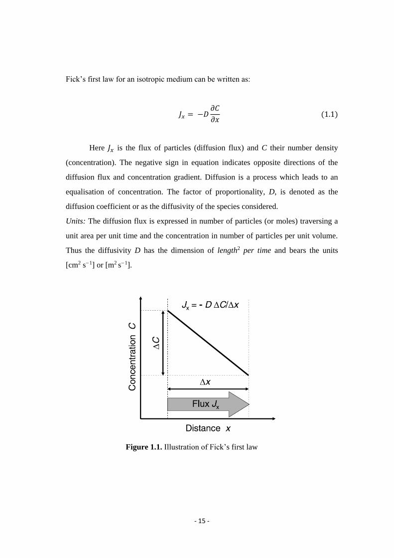
Fick’s first law for an isotropic medium can be written as:
𝐽𝑥 = −𝐷𝜕𝐶
𝜕𝑥 (1.1)
Here 𝐽𝑥 is the flux of particles (diffusion flux) and C their number density
(concentration). The negative sign in equation indicates opposite directions of the
diffusion flux and concentration gradient. Diffusion is a process which leads to an
equalisation of concentration. The factor of proportionality, D, is denoted as the
diffusion coefficient or as the diffusivity of the species considered.
Units: The diffusion flux is expressed in number of particles (or moles) traversing a
unit area per unit time and the concentration in number of particles per unit volume.
Thus the diffusivity D has the dimension of length2 per time and bears the units
[cm2 s−1] or [m2 s−1].
Figure 1.1. Illustration of Fick’s first law

- 16 -
Fick’s first law is easily generalized to three dimensions using a vector notation:
𝐽 = −𝐷 𝐶 (1.2)
The vector of the diffusion flux J is directed opposite in direction to the
concentration gradient vector 𝐶. The nabla symbol, , is used to express the vector
operation on the right-hand side. The nabla operator acts on the scalar concentration
field C(x, y, z, t) and produces the concentration-gradient field 𝐶. The
concentration-gradient vector always points in that direction for which the
concentration field undergoes the most rapid increase and its magnitude equals the
maximum rate of increase of concentration at the point. For an isotropic medium the
diffusion flux is antiparallel to the concentration gradient.
Usually, in diffusion processes the number of diffusing particles is conserved.
Let us choose an arbitrary point P located at (x, y, z) and a test volume of size Δx, Δy,
and Δz (Figure 1.2).
Figure 1.2. Infinitesimal test volume. The in- and outgoing y-components of the
diffusion flux are indicated by arrows.

- 17 -
The diffusion flux 𝐽 and its components 𝐽𝑥, 𝐽𝑦, 𝐽𝑧 vary across the test volume.
If the sum of the fluxes leaving and entering the test volume do not balance, a net
accumulation (or loss) must occur. This material balance can be expressed as
inflow - outflow = accumulation (or loss) rate.
The flux components can be substituted into this equation to yield
[𝐽𝑥(𝑃) − 𝐽𝑥(𝑃 + 𝑥)]𝑦𝑧 +
[𝐽𝑦(𝑃) − 𝐽𝑦(𝑃 + 𝑦)]𝑥𝑧 +
[𝐽𝑧(𝑃) − 𝐽𝑧(𝑃 + 𝑧)]𝑥𝑦 = accumulation (or loss) rate.
Using Taylor expansions of the flux components up to their linear terms, the
expressions in square brackets can be replaced by Δx∂Jx/∂x, Δy∂Jy/∂y, and Δz∂Jz/∂z,
respectively. This yields:
− [𝜕𝐽𝑥
𝜕𝑥+
𝜕𝐽𝑦
𝜕𝑦+
𝜕𝐽𝑧
𝜕𝑧]𝑥𝑦𝑧 =
𝜕𝐶
𝜕𝑥𝑥𝑦𝑧 (1.3)
where the accumulation (or loss) rate in the test volume is expressed in terms of the
partial time derivative of the concentration. For infinitesimal size of the test volume,
Equation (1.3) can be written in compact form by introducing the vector operation
divergence , which acts on the vector of the diffusion flux:
− 𝐽 =𝜕𝐶
𝜕𝑡 (1.4)
1.1.1.2 Fick’s Second Law
By combination of above mentioned equations, we can get the following:

- 18 -
𝜕𝐶
𝜕𝑡= (𝐷 𝐶) (1.5)
From the mathematical point of view Fick’s second law is a second-order partial
differential equation. It is non-linear if D depends on concentration, which is, for
example, the case when diffusion occurs in a chemical composition gradient. The
composition-dependent diffusivity is usually denoted as the interdiffusion coefficient.
If the diffusivity is independent of concentration, which is the case for tracer
diffusion in chemically homogenous systems or for diffusion in ideal solid solutions,
the equation above can be simplifies to:
𝜕𝐶
𝜕𝑡= 𝐷 𝐶 (1.6)
where Δ denotes the Laplace operator. This form of Fick’s second law is sometimes
also called the linear diffusion equation. It is a linear second-order partial differential
equation for the concentration field C(x, y, z, t). One can strive for solutions of this
equation, if boundary and initial conditions are formulated.
1.1.2. Random Walk Theory
From a microscopic point of view, diffusion occurs by the Brownian motion
of atoms or molecules. As already mentioned above, Albert Einstein in 1905 [2]
published a theory for the chaotic motion of small particles suspended in a liquid.
Einstein argued that the motion of these particles is due to the presence of molecules
in the fluid. He further pointed that molecules due to their Boltzmann distribution of
energy are always subject to thermal movements of a statistical nature. According to
Einstein stochastic motions occur in matter all the way down to the atomic scale. He
related the mean square displacement of particles to the diffusion coefficient. The

- 19 -
same relation was developed nearly the same time by the Polish scientist
Smoluchowski. [3, 4] Nowadays it is called the Einstein relation or the Einstein-
Smoluchowski relation.
In gases, diffusion occurs by free flights of atoms or molecules between their
collisions. The individual path lengths of these flights are distributed around some
well-defined mean free path. Diffusion in liquids exhibits more subtle atomic motion
than gases. Atomic motion in liquids can be described as randomly directed shuffles,
each much smaller than the average spacing of atoms in a liquid. Most solids are
crystalline and diffusion occurs by atomic hops in a lattice, due to many individual
displacements (jumps) of the diffusing particles. Diffusive jumps are usually single-
atom jumps of fixed lengths, the size of which is of the order of the lattice parameter.
Jump processes are promoted by thermal activation. Usually an Arrhenius law holds
for the jump rate Γ:
𝛤 = 𝜈0𝑒𝑥𝑝 (−𝐺
𝐾𝐵𝑇) (1.7)
The prefactor 𝜈0 denotes an attempt frequency of the order of the Debye frequency
of the lattice. 𝐺 is the Gibbs free energy of activation, 𝐾𝐵 the Boltzmann constant,
and T the absolute temperature. Details can be found in a review by Haenggi et al.
[5] and in the textbook of Flynn. [6]
1.1.2.1. Simplified model
Before going through more rigorous mathematical solutions of random walks,
it may be helpful to look at a simple situation: unidirectional diffusion of interstitials
in a simple cubic crystal. Let us assume that the diffusing atoms are dissolved in low
concentrations and that they move by jumping from an interstitial site to a

- 20 -
neighboring one with a jump length λ as demonstrated in Figure 1.3. We suppose a
concentration gradient along the x-direction and introduce the following definitions:
Γ: jump rate (number of jumps per unit time) from one plane to the neighboring one,
n1: number of interstitials per unit area in plane 1,
n2: number of interstitials per unit area in plane 2.
Without a driving force, forward and backward hops occur with the same jump rate
and the net flux J from plane 1 to 2 is
𝐽 = 𝛤𝑛1 − 𝛤𝑛2 (1.8)
The quantities n1 and n2 are related to the volume concentrations (number densities)
of diffusing atoms via
𝐶1 = 𝑛1
, 𝐶2 =
𝑛2
(1.9)
Usually in diffusion studies the concentration field, C(x, t), changes slowly as a
function of the distance variable x in terms of interatomic distances. From a Taylor
expansion of the concentration-distance function, keeping only the first term (Figure
1.3), we get
𝐶1 − 𝐶2 = −𝜕𝐶
𝜕𝑥 (1.10)

- 21 -
Inserting Equations (1.9) and (1.10) into Eq. (1.8) we get
𝐽 = −2𝛤𝜕𝐶
𝜕𝑥 (1.11)
By comparison with Fick’s first law we obtain for the diffusion coefficient
𝐷 = 𝛤2 (1.12)
Taking into account that in a simple cubic lattice the jump rate of an atom to one of
its six nearest-neighbor interstices is related to its total jump rate via Γtot = 6Γ, we
obtain:
Figure 1.3. Schematic representation of unidirectional diffusion of atoms in a
lattice

- 22 -
𝐷 =1
6𝛤𝑡𝑜𝑡
2 (1.13)
This equation shows that the diffusion coefficient is essentially determined by the
product of the jump rate and the jump distance squared.
1.2. Motivation
As we saw from previous subchapter, diffusion is not a simple process even
when relatively simple homogeneous systems are considered. On other hand,
understanding the mechanism of the diffusion of small molecules, macromolecules
and nanoparticles in complex, nanostructured environments is of paramount
fundamental and technological importance. Indeed, diffusion is often the dominant
mechanism for the transport of such species in e.g. solid nano-porous structures,
polymer solutions and gels or living cells. Thus, it is relevant for many processes and
applications including drug delivery, cell nutrition, porous chromatography, polymer
synthesis and separation, treatment of waste water, oil recovery, mineral processing,
drying of paints, production of personal care products, etc. Not surprisingly
therefore, studying the penetrant diffusion and correlating it to the chemical, physical
and topological characteristics of the nanostructured environment had become a
major research topic in various fields spanning from polymer physics to cell biology.
A number of theories, models and empirical relations have been introduced to
describe the diffusion of small species in polymer systems, in intercellular matrices
or in solid periodic nano-porous structures.
During last decades a lot of techniques have been developed to study
diffusion process. Mostly used ones are: pulse-field-gradient NMR (PFG-NMR),
forces Rayleigh scattering (FRS), dynamic light scattering (DLS), fluorescence

- 23 -
recovery after photobleaching (FRAP), etc. [7-9]. All the mentioned technics have
specific advantages but also some limitations. For example they may require
relatively high concentration of the tracer to enhance signal to noise ratio, however
the local properties might significantly change due to high amount of these tracers. In
addition the main disadvantage of these techniques is the large probing volume and
thus the lack of ability to address the local dynamics in heterogeneous systems,
which may be of crucial importance.
Recently Fluorescence Correlation Spectroscopy (FCS) has emerged as a
powerful tool to investigate the diffusion of fluorescent molecules, macromolecules
or nanoparticles in various environments. Detailed description on working principle
of FCS is given in chapter 2. For decades FCS has been limited mostly to biological
studies, i.e. aqueous environments. [10-15] Only recently FCS was successfully
applied to study the size and conformation of macromolecules in organic solvents
[16, 17] , in gels [18, 19], in polymer solutions and melts [20-25] and polymer blends
[26].
By studying the diffusion of the small molecules in different systems, first
one obtains information about the molecule itself: how it is diffusing in different
environment, does it have any interaction with the system, what forces drive this
molecule to diffuse and so on. Second, information about the properties of the system
in which the molecule is diffusing can be obtained: i.e. the viscosity, the length scale
of the possible heterogeneities, does system change it properties in time.
In my thesis I will describe both above mentioned phenomena. In the chapter
3 I will show, how by using FCS and studying the diffusion of small tracer molecules
one can obtain information about the local properties of the environment and thus
track the phase separation kinetics in polymer blend. Here the very small probing
volume of the FCS (<1µm3) allows looking in individual domains of a heterogeneous
structure. In chapter 4 I will demonstrate that even when the length scale of the
heterogeneities becomes smaller than the FCS probing volume one can still obtain
- 24 -
important microscopic information by studying small tracer diffusion. To this end I
will introduce a system of star shaped polymer solutions and show that the mobility
of small molecular tracers on microscopic level, is almost unaffected by the
transition of the polymer system to a “glassy” macroscopic state. Finally, in chapter
5, I go beyond simply monitoring the diffusion, and describe the design of a system
that combines two levels of nanoporosity and allows control of the diffusion of tracer
molecules.

- 25 -
CHAPTER 2
Methods
2.1. Confocal Laser Scanning Microscopy
The confocal microscope was invented by Marvin Minsky [27] in 1957 at
Harvard University. The lateral resolution it offers is only slightly improved in
comparison to conventional wide field fluorescence microscopy. However, what
really sets the confocal microscope apart from its wide field counterpart is its far
superior axial resolution, allowing thin sections through a sample to be imaged.
In addition the confocal microscope allows almost all out of focus fluorescence to be
omitted. This greatly improved image contrast and quality. Figure 2.1 (Images taken
from [28]) below shows a comparison of wide field and confocal images.
Combined with improvements in laser technology, the confocal microscope
has allowed imaging of living samples that could not have been imaged by
conventional optical microscopy or electron microscopy. It has been also utilized in
multi-disciplinary sciences to study photo-luminescence [29] in semi-conductor
films, bioluminescent interaction with nanoparticles. [30] In the pharmaceutical
industry, it was recommended to follow the manufacturing process of thin film
pharmaceutical forms, to control the quality and uniformity of the drug distribution.
[31]
2.1.1. Operational Principle
The improvements gained by the confocal microscope arise from its system
of illumination and detection of fluorescence. In comparison to wide field

- 26 -
fluorescence microscopy where the entire field of view is illuminated, excitation in
the confocal microscope is achieved by point illumination.
Typically a laser beam is tightly focused by a microscope objective to a diffraction
limited focal spot and this spot is raster scanned across the sample (Figure 2.2). [28]
Figure 2.2. Illustration of confocal excitation and widefield illumination of a
fluorescent sample.
Figure 2.1. Top: Images acquired in wide field mode. Bottom: A single section
acquired in confocal mode showing the increased image detail achievable when
the out of focus background is eliminated.
- 27 -
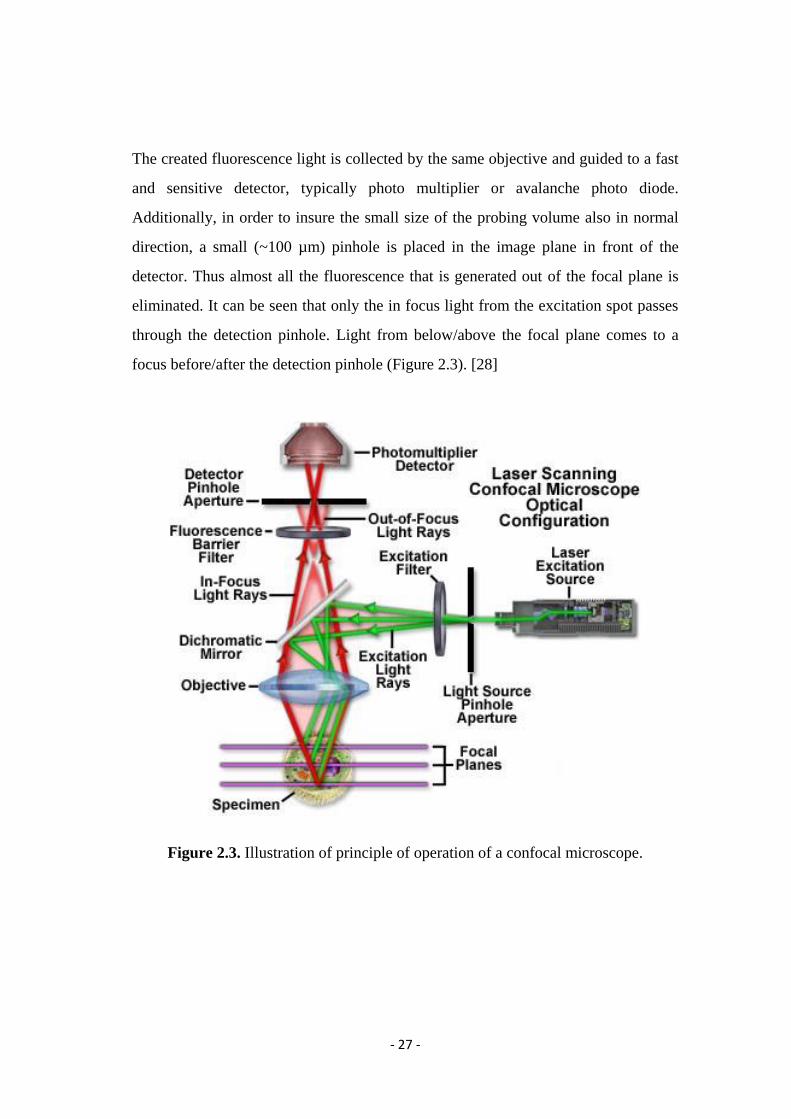
The created fluorescence light is collected by the same objective and guided to a fast
and sensitive detector, typically photo multiplier or avalanche photo diode.
Additionally, in order to insure the small size of the probing volume also in normal
direction, a small (~100 µm) pinhole is placed in the image plane in front of the
detector. Thus almost all the fluorescence that is generated out of the focal plane is
eliminated. It can be seen that only the in focus light from the excitation spot passes
through the detection pinhole. Light from below/above the focal plane comes to a
focus before/after the detection pinhole (Figure 2.3). [28]
Figure 2.3. Illustration of principle of operation of a confocal microscope.

- 28 -
2.1.2. Resolution
The confocal microscope is an optical microscope and therefore its resolution
is limited by diffraction. This means a point source is not imaged to a single point in
the image plane. There are many definitions of resolution in use in optical
microscopy. Qualitatively it is the minimum separation of two point sources which
can still be distinguished [30]. The size of the spot that is formed in the image plane
is governed by the wavelength of the light, , and the numerical aperture (NA) of the
lens. The NA is calculated from (2-1) and is governed by the semi-angle and the
refractive index of the medium, n.
𝑁𝐴 = 𝑛 ∙ sin 𝛼 (2.1)
Due to the diffraction of the light with conventional means one cannot achieve lateral
size of the observation volume smaller than roughly half of the wavelength of the
light used [32]
𝑟0 = 1.22
2𝑁𝐴𝑜𝑏𝑗 (2.2)
In addition, in axial direction resolution is much worse [32]
𝑧0 =1.5𝑛
𝑁𝐴𝑜𝑏𝑗2 (2.2)
where λ – wavelength of the light, NAobj – numerical aperture of the objective, n –
refractive index of the medium.

- 29 -
2.1.3. Laser Illumination and Fluorescence
The laser provides an intense source of light at a specific wavelength. Lasers
suitable for confocal microscopy are available in a wide range of wavelengths [29]
from near infrared to ultraviolet.
To obtain diffraction limited excitation spot the whole of the back focal
aperture of the objective must be uniformly illuminated. Practically this is achieved
by expanding the laser beam to completely fill the back focal aperture of the
objective. When the beam is the same size as the back focal aperture the objective it
is said to be fully filled. The laser beam will not have a uniform beam profile though;
it is more likely to be approximately Gaussian. [33] By further expanding the beam
and only using the central portion a more uniform beam profile is presented to the
objective lens, although this is at the expense reduced transmitted light. [30]
The most common and useful imaging mode used in confocal microscopy is
the fluorescence mode. Samples are stained or prepared to contain fluorescent tags or
molecules.
The major problem with fluorophores is that they fade (irreversibly) when
exposed to excitation light (Figure. 8). Although this process is not completely
understood, it is believed that it to occur when fluorophore molecules react with
oxygen or oxygen radicals and become nonfluorescent. [34-36] The reaction can take
place after a fluorophore molecule transitions from the singlet excited state to the
triplet excited state. Although the fraction of fluorophores that transitions to the
triplet state is small, its lifetime is typically much longer than that of the singlet state.
This can lead to a significant triplet state fluorophore population and thus to
significant photobleaching. [37] Some strategies have been developed to reduce the
rate of photobleaching. [36, 37] One of the approaches is to reduce the amount of
oxygen that would react with the triplet excited states. And this can be easily done by
displacing it using an inert gas. [37] Another approach is to use the free-radical

- 30 -
scavengers to reduce the oxygen radicals. Shortening the long lifetime of the triplet
excited state has also been shown to be effective. [38] Other ways include using a
high numerical aperture lens to collect more fluorescence light and thus use less
excitation light. [39] Also, keeping the magnification as low as is permissible spreads
the excitation light over a larger area, thereby reducing the local intensity. While
photobleaching makes fluorescence microscopy more difficult, it is not always
undesirable. One technique that takes advantage of it is fluorescence recovery after
photobleaching (FRAP). [9] It involves exposing a small region of the specimen to a
short and intense laser beam, which destroys the local fluorescence, and then
observing as the fluorescence is recovered by transport of other fluorophore
molecules from the surrounding region. Quantities such as the diffusion coefficient
of the dyed structures can then be determined. [40]
2.1.4. LSCM setup used in this work
Imaging of polymer blends was made with a commercial setup consisting of
an inverted microscope (IX70) and a confocal laser scanning unit, FluoView FV300
(Olympus, Japan). Either a PLAPON 60× oil immersion objective (1.45 NA, 100 µm
working distance) or a MPLAPO 50× dry objective (0.95 NA, 300 µm working
distance) were used, respectively, for the room temperature and elevated temperature
studies. The fluorescein dyes attached to the PS chains were excited with the 488 nm
line of a 20 mW Argon laser fiber coupled to the laser scanning unit. Fluorescence
images were recorded using a LP 505 long-pass emission filter. The microscope
cover glasses with the deposited polymer blend samples were mounted in an
Attofluor steel chamber (Invitrogen) with the polymer film pointing upwards for the
room temperature studies. For studies at elevated temperature the cover glasses were
mounted on a THMS 600 heating stage (Linkam) with the polymer film pointing
down i.e. towards the microscope objective. The obtained LSCM images were

- 31 -
analyzed using the “imageJ” software package, including the “LOCI” and “Radial
Profile” plugins. The same software with appropriate thresholds was used in
obtaining the number of grains, their average size and area as a function of time.
2.2. Fluorescence Correlation Spectroscopy (FCS)
2.2.1. Introduction to FCS
FCS was first described in the early 1970s in a series of classic papers. An
extensive description and its application can be found in recent publications. [10-19]
FCS is based on the analysis of time-dependent intensity fluctuations that are the
result of some dynamic process, typically translational diffusion into and out a small
observation volume, defined by a focused laser beam and a confocal aperture. When
the fluorophore diffuses into a focused light beam, there is a burst of emitted photons
due to multiple excitation-emission cycles from the same fluorophore. If the
fluorophore diffuses rapidly out of the volume photon burst is short lived. In case of
slow diffusion the photon burst displays a longer duration. By correlation analysis of
the time-dependent fluctuations of the emission signal, one can determine the
diffusion coefficient of the fluorophore.
In addition to translational diffusion, intensity fluctuations can occur due to
ligand-macromolecule binding, rotational diffusion, intersystem crossing and exited
state reactions. [41-43] Different equations are needed to describe each process, and
usually two or more processes affect the data at the same time. Also important is to
account for the size and shape of the observation volume. As a result, the theory and
equations for FCS are rather complex.

- 32 -
2.2.2. Principle of FCS
On Figure 2.4 schematic drawing of Fluorescence Correlation Spectroscopy
setup is presented. The scheme is very similar to that of a confocal microscopy
described above. Excitation is usually accomplished with a laser focus to a
diffraction-limited spot using high numerical aperture objective. When the
fluorescent species enter this spot, they are exited and the emitted fluorescence is
collected by the same objective, passing through the dichroic mirror and emission
filters. A confocal pinhole is used to reject out of focus signal.
Afterwards, the light is reaching a detector, usually avalanche photodiode
(APD) or photomultiplier (PMT) with single photon sensitivity.
Using these optical conditions, an ellipsoidal observation volume is created
that is elongated along the optical axis, with the main axis of r0 and z0 with the rough
size of 0.2 m and 1 m respectively, i.e. with total volume of less than a 1fl=10-15
liters. The average number of fluorophores in the volume is determined by their bulk
concentration and remains constant in a stationary experiment. If the fluorophore
concentration is 1nM (that is a typical value used in experiments), then the
observation volume contains less than 0.6 molecules in average. When the
Figure 2.4. Schematic drawing of Fluorescence Correlation Spectroscopy

- 33 -
fluorophores diffuse in and out of the observation volume, they cause fluorescence
intensity fluctuations. The intensity at a given time F(t) is compared with the
intensity at a given time F(t+). If the diffusion is slow F(t) and F(t+) are likely to
be similar. In case of fast diffusion, F(t) and F(t+) are likely to be different.
For obtaining quantitative information about the diffusion process, these
fluctuations can be analyzed in terms of fluorescence intensity autocorrelation
function (ACF). [44, 45]
The fluorescence intensity autocorrelation function G() can be expressed by
using the fluorescent light intensity fluctuations δF(t) as follows:
𝐺() = ⟨𝐹(𝑡) 𝐹(𝑡 + )⟩
⟨𝐹(𝑡)⟩2 2.3
On Figure 2.5 (taken from [46]) it is shown how the autocorrelation curve can
be schematically constructed. The brackets ⟨ ⟩ indicate the time average over the
fluorescence signal, t is the time at which the fluorescent intensity is recorded and
is the correlation lag time. The above formula is integrated and normalized: [47, 48]
𝐺() = ⟨[⟨𝐹(𝑡)⟩ + 𝐹(𝑡)] [⟨𝐹(𝑡)⟩ + 𝐹(𝑡 + )]⟩
⟨𝐹(𝑡)⟩2
= ⟨𝐹(𝑡)⟩2 ⟨𝐹(𝑡) 𝐹(𝑡 + )⟩
⟨𝐹(𝑡)2⟩ 2.4
= 1 + ⟨𝐹(𝑡) 𝐹(𝑡 + )⟩
⟨𝐹(𝑡)⟩2
Where F(t) = F(t) − F(t) , because F(t) gives the corresponding fluorescent fluctuations in
the fluorescent signal F(t) around the mean value ⟨𝐹(𝑡)⟩. And ⟨𝐹(𝑡) ⟨𝐹(𝑡)⟩⟩ =
⟨⟨𝐹(𝑡)⟩ 𝐹(𝑡)⟩ = 0, since ⟨𝐹(𝑡)⟩ = 0

- 34 -
2.2.3. Autocorrelation function
In order to extract information, such as concentration, diffusion coefficient,
reaction rate constant, from the measured autocorrelation functions one has to fit it
with a theoretical correlation function. There are several reviews concerning the
theories of the autocorrelation functions. [45, 49-51]
2.2.3.1 Autocorrelation function for single type of species
Autocorrelation function G() for single type of fluorescent species with
diffusion coefficient D and molar concentration c is: [49]
Figure 2.5. Schematic representation of autocorrelation curve formation in the lag
time, t. in Fluorescence Correlation Spectroscopy

- 35 -
𝐺() = 1 +1
𝑐 𝑉𝑒𝑓𝑓
1
(1 +4𝐷0
2 )
1
√1 +4𝐷𝑧0
2
2.5
where 𝑉𝑒𝑓𝑓 is the effective observation volume, which depends on the geometry of
the focus for excitation and emission. Commonly it is approximated with 3
dimensional Gaussian profile with 0 and 𝑧0
are the half-widths in x-y plane and in
the z direction, respectively. These parameters can be obtained from calibration
measurements with a solution of fluorophores having known diffusion coefficient.
By putting average particle number 𝑁 = 𝑐 𝑉𝑒𝑓𝑓, the effective diffusion time 𝐷 =
0 2 4𝐷⁄ , and the structure parameter 𝑘 = 0
𝑧0 ⁄ in the equation above, we will get:
𝐺() = 1 +1
𝑁
1
(1 +𝐷
)
1
√1 +
𝑘2𝐷
2.6
The diffusion coefficient D is related to the size of the fluorescent molecules via the
Stokes-Einstein equation:
𝐷 =𝑘𝑇
6𝑅 2.7
Where k is the Bolzmann constant, T is the absolute temperature, is the viscosity of
the medium and R is the hydrodynamic radius of the molecule.
2.2.3.2 Autocorrelation function for multiple types of species
In case of several types of noninteracting fluorescent species diffusing in the
observation volume with different diffusion coefficients, the fluorescence intensity

- 36 -
autocorrelation function is the sum of the contributions of the individual species. The
𝐺() for the mixture of m of different fluorescent species is given by:
𝐺() = 1 +1
𝑁∑ 𝑝
𝑖𝑔
𝑖()
𝑚
𝑖=1
2.9
Where 𝑔𝑖() =1
(1+
𝐷𝑖)
1
√1+
𝑘2𝐷𝑖
and 𝑝𝑖 =𝑖
2𝑐𝑖
∑ 𝑖2𝑐𝑖
𝑚𝑖=1
In the equation above, 𝑝𝑖 is the relative amplitude of the molecules with distinct
diffusion coefficients, 𝑐𝑖 is the concentration of these molecules and 𝑖 is the
fluorescent brightness of species i. [52]
2.2.4 Fluorescence excitation and emission spectra. Jablonski
diagram
Fluorescence is the emission of photons by atoms or molecules whose
electrons are transiently stimulated to a higher excitation state by radiant energy from
an outside source. When a fluorescent molecule absorbs a photon of the appropriate
wavelength, an electron is excited to a higher energy state and almost immediately
returns back to its initial ground state. In the process of energy collapse the molecule
can release the absorbed energy as a fluorescent photon. Since some energy is lost in
the process, the emitted fluorescent photon typically exhibits a lower frequency of
vibration and a longer wavelength than the excitatory photon that was absorbed. This
can be graphically illustrated in Figure 2.6., and is known as a Jablonski diagram.
Jablonski diagrams are often used as the starting point for discussion light absorption
and emission. To illustrate various molecular processes that can occur in exited
states. The diagrams are named after Professor Alexander Jablonski, who is regarded

- 37 -
as the father of fluorescence spectroscopy because of his many accomplishments,
including description of concentration depolarization and defining the term
“anisotropy” to describe the polarized emission from solutions.
There are two categories of excited states - the singlet excited state and the
triplet excited state. Most commonly, an excited electron occupies an excitation level
within the singlet excited state, and when it returns to the ground state, energy can be
given up as fluorescence emission. Alternatively, energy can be given up as heat
(internal conversion), in which case no photon is emitted. When excited above the
ground state, there is also a probability that an electron enters the triplet excited state.
Figure 2.6. Jablonski diagram showing energy levels occupied by an excited
electron

- 38 -
Molecules with electrons in this state are chemically reactive, which can lead to
photobleaching and the production of damaging free radicals.
In case of fluorescence, the absorption and re-emission events occur nearly
simultaneously, within the interval of 10-9–10-12 seconds; therefore, fluorescence
stops the moment there is no more exciting incident light. There is also possibility
that the period between excitation and emission lasts longer and can take from a
second to minutes; such emission process is called phosphorescence.
Molecules that are capable of fluorescing are called fluorescent molecules,
fluorescent dyes, or fluorochromes. Fluorochromes exhibit distinct excitation and
emission spectra that depend on their atomic structure and electron resonance
properties. Molecules absorb light and re-emit photons over a spectrum of
wavelengths (the excitation spectrum) and exhibit one or more characteristic
excitation maxima (Figure 2.7.)
Figure 2.7. Normalized absorption and fluorescence emission spectra of
fluorescent dye.

- 39 -
Absorption and excitation spectra are distinct but usually overlap, sometimes to the
extent that they are nearly indistinguishable. However, for many fluorescent dyes
like Fluorescein, Alexa, Rhodamine, the absorption and excitation spectra are clearly
distinct. The widths and locations of the spectral curves are important, particularly
when selecting two or more fluorochromes for labeling different molecules within
the same specimen.
Finally, the shapes of spectral curves and the peak wavelengths of absorption and
emission spectra vary, depending on factors contributing to the chemical
environment of the system, including pH, ionic strength, solvent polarity, O2
concentration, presence of quenching molecules, and others. This fact explains why
the fluorescence of a dye such as fluorescein varies depending on whether it is free in
solution or conjugated to a protein or other macromolecule.
2.2.5. Fluorescent Dyes
Initially FCS measurements were done by using fluorophores that are already
known from fluorescence spectroscopy and microscopy techniques. [53] As
described above FCS is a single molecule technique and the high quantum efficiency,
large absorption cross section and photostability are the key requirements of
fluorophores for such techniques. For aqueous systems Fluorescein and Alexa dye
family exhibits a large selection of different colors with absorption maxima ranging
from 350 nm to 750 nm, covering more than the visible spectrum. For the non-
aqueous systems, chromospheres which are dissolved in organic solvents are usually
used. Such are rylene family dyes. Because of the very good photostability and high
quantum yield [54, 55] they are suitable dyes for the FCS studies.
In this work I used in-house synthesized N, N´-bis(2,6-Diisopropylphenyl)-1,6,9,14-
tetraphenoxyterrylene-3,4:11,12-tetracarboxi-diimide, a terrylene (TDI) dye, to study
the dynamics of the phase separation process in polymer blends and also to study
mobility of the small tracer in glassy star-shaped polymer solutions. In one of the

- 40 -
projects I used the commercially available Alexa Fluor 488 and Alexa Fluor 647
(Invitrogen, Karlsruhe, Germany) to study the diffusion in PNIPAM modified Silica
Inverse Opals. The chemical structures of the dyes are given in Figure 2.8.
(b) Alexa Fluore 488
(a) Terrylene (TDI)
(c) Alexa Fluore 647
Figure 2.8. Molecular structure of the fluorescent dyes (a) Alexa Fluore 488, (b)
Terrylene (TDI), (c) Alexa Fluore 647
(d)
- 41 -
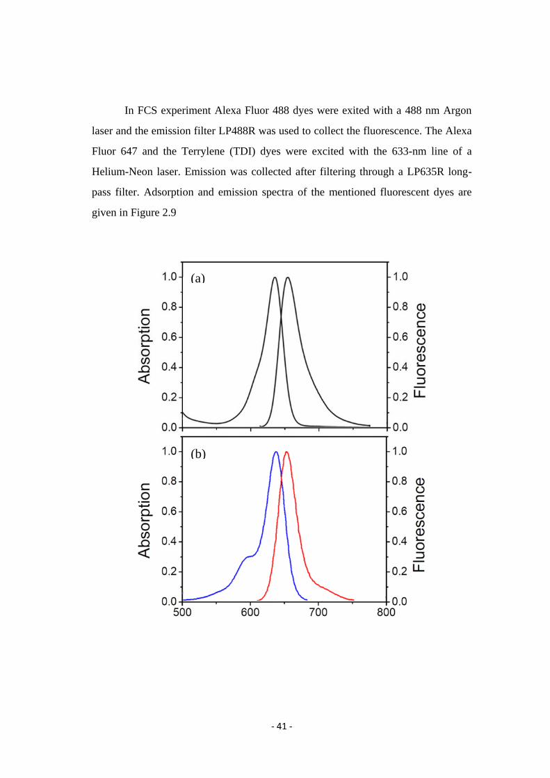
In FCS experiment Alexa Fluor 488 dyes were exited with a 488 nm Argon
laser and the emission filter LP488R was used to collect the fluorescence. The Alexa
Fluor 647 and the Terrylene (TDI) dyes were excited with the 633-nm line of a
Helium-Neon laser. Emission was collected after filtering through a LP635R long-
pass filter. Adsorption and emission spectra of the mentioned fluorescent dyes are
given in Figure 2.9
(a)
(b)

- 42 -
2.2.6. FCS Setup used in this work
The FCS measurements were performed on a commercial setup based on the
Olympus laser scanning confocal microscope described in (2.1.4) that was extended
with a fiber coupled FCS unit (Pico Quant, Germany). For the studies of the inverse
opals filled with aqueous solutions, a 60x water immersion objective with numerical
aperture of 1.2 and 200 μm working distance was used. Since the inverse opal layer
was a relatively thin film with some cracks and defects, a LSCM was performed
prior to the FCS measurement to identify appropriate position of the inverse opal
layer. At each position a series of 10 measurements with a total duration 5 min was
performed.
2.3. Scanning electron microscopy (SEM)
In scanning electron microscopy (SEM), an electron beam is used to map the
(c)
Figure 2.9. Absorption and fluorescent emission spectra of the following dyes (a)
Alexa Fluore 488, (b) Alexa Fluore 647, (c) Terrylene (TDI)
(e)

- 43 -
surface of a specimen. [56, 57] An electron beam with energy of few keV is emitted
by a cathode (gun) and focused by condenser lenses. The beam is used to scan a
rectangular area of the specimen line-by-line. The electrons interact with the atoms at
or near the sample surface depending on the acceleration voltage. Back-scattered or
secondary electrons are detected by specialized detectors. This signal is amplified
and yields a magnified black and white image of the sample surface with resolutions
in the nm range (and below). Different grey scale values in the SEM image arise
from differences in the electron densities of the materials. Elements of higher atomic
number appear brighter than those of lower atomic number.
2.4. Vertical deposition (VD) method
The assembly of colloids into well-defined structures occurs under the
influence of external fields, e.g., gravitational sedimentation, [58] electrophoretic
deposition, [59] or vertical deposition either by evaporation [60] or lifting the
substrate. [61] In the vertical lifting deposition method when a hydrophilic substrate
is immersion into a colloidal dispersion a meniscus is formed at substrate water
interface. At the three phases contact lines (air, dispersion, and substrate) evaporation
takes place and this causes a solvent flux towards the meniscus, as shown in Figure
2.10.
Thus, colloidal particles are constantly transported with the liquid to the
crystallization front. An interplay of long-range attractive and short-range repulsive
forces causes the self-assembly of the colloidal material into a face-centered cubic or
hexagonally close packed crystal. [62, 63]
In order to control the thickness of such a colloidal crystal, some parameters
should be optimized. The substrate is withdrawn from the dispersion at a certain
speed at given at curtain temperature and humidity.

- 44 -
Alongside with this research, also the counterpart to the highly ordered
crystals - colloidal glasses [64] - comprising of two distinct, monodisperse latex
particles have already been developed. [65] Doping of the colloidal crystal with
removable moieties (sacrificial templates) opens a pathway to the designed
introduction of defects, which are highly interesting with respect to their contribution
to phononic properties. At the same time, colloidal crystals and glasses serve as
templates for the fabrication of so-called inverse opals. [66] These materials exhibit a
highly ordered interconnected 3D network with high surface area, since the
constituent spheres of the colloidal crystals have been removed.
2.5. Polymer grafting methods
2.5.1. “Grafting-from”
In a “grafting‐from” approach a polymer brushes are obtained by “growing”
Figure 2.10. Schematic draw of the colloidal crystallization process in a vertical
lifting deposition apparatus.

- 45 -
the polymer away from the surface (Figure 2.11a). This is usually done using an
initiator functionalized surface and polymerization of the monomer on top of the
surface. There are numerous polymerization methods working in this way. [67, 68]
In recent years “grafting‐from”‐techniques using living radical polymerization,
especially ATRP (Chapter 2.4.3), have become popular. This is due to the ability to
obtain grafted polymers with narrow molecular weight distributions and
straightforward experimental procedures. [68-71]
The biggest advantage of the "grafting‐from" technique is the very high
grafting density of the obtained polymer brushes. During the polymerization the
already polymerized monomer is swollen by the monomer/solvent solution. This
allows the monomer to freely diffuse to the growing chain end and continue the
reaction. Only at high grafting densities and molecular weight distributions the
diffusion gets hindered and the polymerization is stopped.
2.5.2. “Grafting-to”
In a “grafting‐to” approach a polymer brushes are obtained by attaching an already
polymerized chain with curtain molecular weight to a surface (Figure 2.11b).
(a) (b)
Figure 2.11. Schematic representation of the “grafting-from”(a) and
“grafting-to”
(b) preparation methods for polymer brushes.

- 46 -
To do so, mostly a functionalized polymer is attached to a surface carrying a
complimentary functional group. The biggest advantages are the simple synthesis
and characterization of the used polymers.
Typically, the used polymers are obtained by living polymerization techniques by
using either a functionalized starter or stopping the polymerization with a specific
reactant, the end‐functionalization is achieved. The consecutive “grafting‐to” step
can be performed in solution or melt, where usually higher grafting densities are
obtained. Compared to the “grafting‐from” approach only polymer brushes with
lower grafting densities are achieved.
2.5.3. Atom transfer radical polymerization (ATRP)
The free radical polymerization is one of the most important polymerization
techniques used for production of high molecular weight polymers. [70, 71] A
variety of different monomers can be suited for this type of polymerization and
copolymerization under certain experimental conditions. Typically, the free radical
polymerization can be done in in a high temperature range between the room
temperature and 100 oC under ambient pressure. The polymerization can be carried
out in organic solution, aqueous media or in solvent mixuture. In contrast to the step-
growth polymerization, high molecular weight products are obtained already after
short reaction times and at low conversions. While the most kinds of alkenes
functionalized with hydroxy-, amino- and acid- groups can be used, nearly 50 % of
all commercial polymers are produced by the free radical polymerization. The most
known examples for commercially synthesized polymers via radical polymerization
are ethylene, styrene, vinyl chloride and (meth) acrylates.
One should also mention that the control over the molecular weight and the
polydispersity of the products is difficult as a result of chain transfer and termination
reactions between radicals. While the chain transfer reactions can be suppressed by
- 47 -
the proper choice of reaction conditions, the diffusion driven termination of the free
radicals, namely recombination and disproportionation, can hardly be avoided. In
order to minimize the termination reactions and to obtain the polymers with high
molecular weights, the concentration of radicals is minimized to some ppm. However
still the rate of initiation is much lower than the rate of propagation, thus, the number
of growing chains is very small during the polymerization (~0.1 %). And this leads
to a broad distribution of the chain lengths, and the preparation of polymers with
controlled architecture is not possible using the free radical polymerization.
Controlled living radical polymerization techniques such as atom transfer radical
polymerization (ATRP) [70, 72] allows the synthesis of high molecular weight
polymers of well-defined architecture in the absence of chain transfer or termination
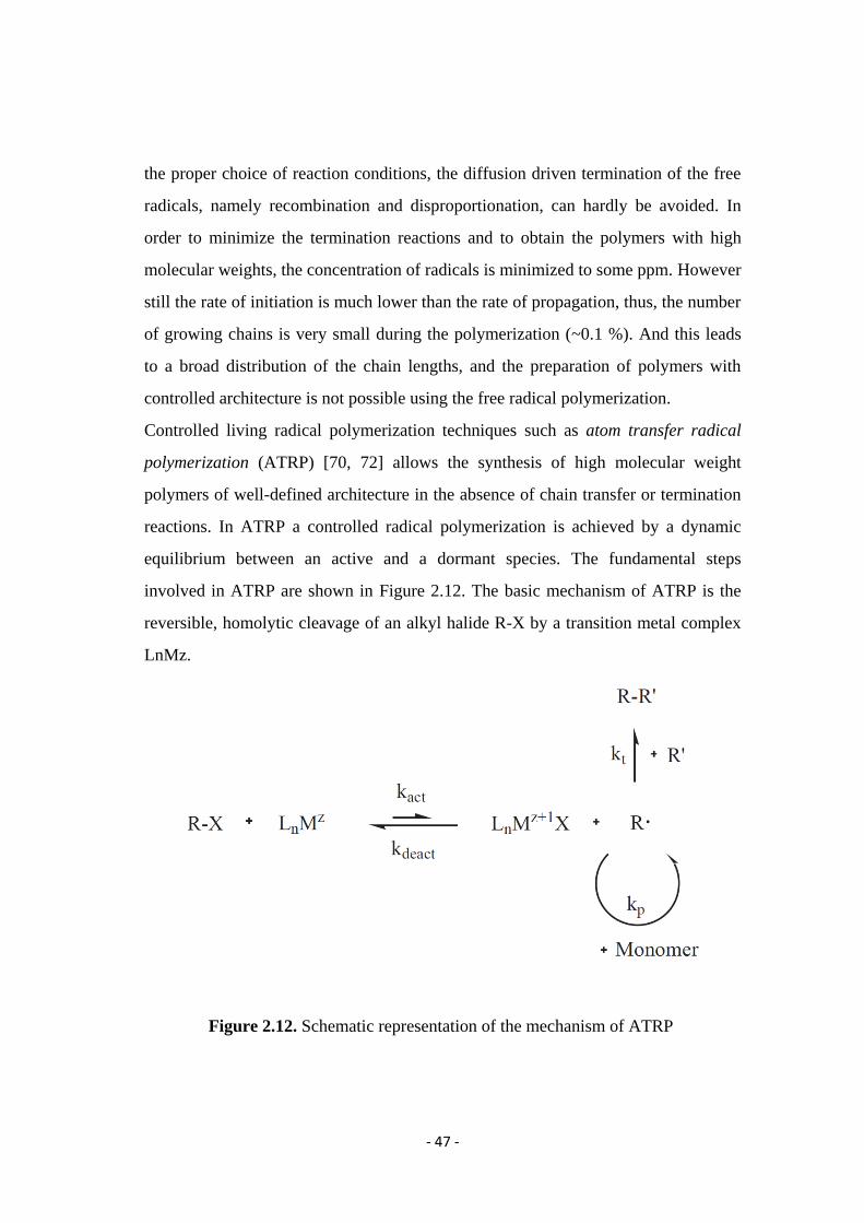
reactions. In ATRP a controlled radical polymerization is achieved by a dynamic
equilibrium between an active and a dormant species. The fundamental steps
involved in ATRP are shown in Figure 2.12. The basic mechanism of ATRP is the
reversible, homolytic cleavage of an alkyl halide R-X by a transition metal complex
LnMz.
Figure 2.12. Schematic representation of the mechanism of ATRP

- 48 -
The transition metal is oxidized, and an alkyl radical is generated. Similar to the free
radical polymerization, the generated radical can attach a monomer or undergo
radical-radical termination. However, in ATRP the rate constant of deactivation kdeact
is much higher than the rate constant of activation kact, favoring the dormant species
rather than the active radical. Thus, by trapping the radical in the dormant form,
which cannot undergo recombination, the radical concentration is reduced. Thus, the
rate constant of termination kt is significantly reduced compared to the rate constant
of propagation kp, and termination reactions are almost completely avoided. After a
certain time in the dormant state, the polymer chain is reactivated and more
monomer can be added. The active species reacts with only a few monomer units
before it is converted back into the dormant form. Thereby, each polymer chain is
active for only a few milliseconds and stays in the dormant state for several seconds.
Typically, in a polymerization this cycle is repeated 1000 times, and a total lifetime
of several hours is achieved. As a result the lifetime of a polymer chain is
significantly increased compared to the free radical polymerization where a growing
polymer chain adds monomer every 1 millisecond and has a lifetime of only 1
second. Additionally, in ATRP the initiation is much faster than in the free radical
polymerization, and all chains are essentially initiated at the same time. For this
reason all the chains grow to identical length, and the product with the low
polydispersity (1.0 < Mw/Mn < 1.5) is obtained. The degree of polymerization X can
be adjusted by the initial monomer to initiator ratio:
𝑋 = [𝑀]0
[𝐼]0
After the polymerization the chains remain active allowing their end-
functionalization and the synthesis of copolymers by sequential monomer addition.

- 49 -
ATRP can be conducted in a wide temperature range from sub-zero to > 100 ◦C. The
list of monomers suitable for ATRP includes styrenes, (meth) acrylates, (meth)
acrylamides, acrylonitrile, vinylpyridine and others. Transition metals like Fe, Ni, Co
are used to mediate the reaction. However, the best results are obtained using copper
catalysts which allows processing of various monomers in a number of different
solvents. Polydentate, N-containing ligands like alkylamines and pyridines are used
to mediate ATRP. [73-75] The ligands increase the solubility of the copper complex
in organic solvents and adjust the atom transfer equilibrium. Usually the chemical
structure of the initiator is similar to the one of the monomer.

- 50 -
- 51 -
CHAPTER 3
Dynamics of phase separation in a polymer blend
3.1. Introduction and Motivation
Spinodal decomposition (SD) [76-80] is widespread phenomenon occurring
in diverse systems: from metallic alloys, to glasses, ceramics, fluid mixtures,
surfactant micellar solutions and in polymer mixtures. The latter are considered as
model systems in studying phase separation kinetics. This is mainly due to their long
characteristic times that allow studying in situ their morphology.
Ideally, one would like to explore the details of the phase separation process
in situ monitoring grain nucleation, dissolution, approach of domains, coalescence,
and growth within the different regimes. In addition, microscopic information on the
interfacial width and of the local composition within the domains is essential.
Apart from different scattering techniques, laser scanning confocal
microscopy (LSCM) has emerged as a powerful tool in studying the morphology of
such heterogeneous systems. LCSM is a non-destructive method and has strong
depth discrimination that is achieved by proper use of a confocal pinhole in the
image plane. In such configuration only light coming from the focal point is detected
and out-of-focus light is rejected thus the images are practically optical sections. As a
result, image processing allows for a 3D visualization of the exact morphology. With
respect to the latter, earlier efforts provided 3D images of bicontinuous polymer
blends obtained via SD. [81-86] Subsequent studies tested the calculated structure
factor against the measured one via scattering experiments and found an excellent
agreement. [82, 83] Further LSCM studies in polymer blends include in situ
monitoring the shrinkage of the mixtures during the photo-polymerization process,

- 52 -
[87] the blend surface morphology [88] and the protein-polymer co-localization in a
phase separated polymer blend. [89]
The aim of the present investigation is twofold. First, to monitor the phase separation
process of a polymer blend in real time with LSCM, and second, to obtain
independent information on the purity of phases. For the latter, LSCM is coupled to
fluorescence correlation spectroscopy (FCS).
The chosen system is a polystyrene/poly(methyl phenyl siloxane) (PS/PMPS)
blend. The blend phase separates upon lowering the temperature, thus exhibits an
upper critical solution temperature or UCST. In addition it possesses large dynamic
asymmetry as revealed by the difference between the component glass temperatures,
ΔTg~ 113 K at P=0.1 MPa. The phase behavior has been investigated experimentally
and theoretically both at ambient pressure [90, 91] and more recently at elevated
pressures. [92] In addition, the glass temperature, Tg, of the hard phase (PS),
interferes with the demixing process thus giving rise to pinning of the domain
structure at a certain stage. Specific information on the degree of purity of phases
was provided by probing the dynamics at the segmental level by dielectric
spectroscopy (DS). [92]
3.2 Materials
3.2.1. Sample Preparation
Direct visualization of the phase separation in the PS/PMPS blends using
LSCM requires fluorescent labeling of one of the polymers. Fluorescein labeled
polystyrenes with different molecular weights, PS-12k (Mw=12.2 kg/mol) and PS-2k
(Mw=2.2 kg/mol) were purchased from Polymer Standards Service (PSS, Mainz,
Germany) and were further purified via precipitation in methanol in order to remove
any remaining not covalently attached fluorescein molecules. After purification the

- 53 -
samples were characterized by Gel Permeation Chromatography (PS was used as a
standard, THF as an eluent) that yielded molecular weights and polydispersities that
are shown in Table 3.1. Poly(methylphenyl siloxane) (PMPS) with molecular weight
Mw=2.27 kg/mol was synthesized in house following synthesis and purification
strategy described previously. [93]
Thin films of symmetric PS/PMPS blends (Table 2.2) on microscope cover
glasses were prepared as follows. First, the PS and PMPS were independently
dissolved in toluene and then mixed, e.g. 0.02g of PS in 1g of toluene + 0.02g of
PMPS in 1g toluene. The mixture was stirred for 7-8 h at room temperature. Films
were prepared by casting the blended solution on round microscope cover glasses
with diameter of 25 mm and thickness of 0.15 mm.
Blend NPS NPMPS wPS
PS116/PMPS16 116 16 0.50
PS21/PMPS16 21 16 0.50
Since the thickness of the film should be relatively high to minimize surface effects
on morphology, most of the toluene was evaporated prior casting, i.e. final amount of
mixture
Mw, PS
(g/mol)
NPS
Mw/Mn
(PS)
Mw, PMPS
(g/mol)
NPMPS
Mw/Mn
(PMPS)
12200 116 1.17 2270 16 1.67
2230 21 1.20
Table 2.1. Molecular Characteristics of the Homopolymers
Table 2.2. Molecular characteristics of the blends

- 54 -
≈ 0.1 - 0.2 g. The casted films were dried at ambient condition overnight and for
further 48 h in vacuum at 50°C.
3.2.2. Annealing Process
To follow the phase separation kinetics different specimens from the same
blend were annealed under vacuum at various temperatures (from 60 to 140°C) and
for various times (from 30 min up to 24 h) and then quenched to ambient temperature
and studied by LSCM.
For the FCS studies films containing a terylene dye, N,N’-bis(2,6-diiso-
propylphenyl)-1,6,9,14-tetraphenoxy-terrylene-3,4,11,12-tetra-carboxidiimide (TDI)
were prepared by adding an appropriate amount of a 10-8 M toluene solution of the
dye to the polymer mixture.
3.3. Phase Diagram and Phase separation by LSCM
The type of morphology in polymer blends (spherical or fibrilar dispersed
phase vs. co-continuous phases), depends not only on the volume fraction but also on
the viscosity and elasticity of the components as well as processing conditions. [76-
78, 94] The phase diagram of the studied PS116/PMPS16 blend is shown in Figure 3.1.

- 55 -
The diagram is based on model calculations using a lattice-based equation of state
that account for the effects of compressibility and nonrandom mixing (details in ref [95]).
The PS/PMPS theoretical phase diagram was successfully tested earlier
against experimental data for different symmetric PS/PMPS blends. [96] The type of
morphology in polymer blends (spherical or fibrilar dispersed phase vs. co-
continuous phases), depends not only on the volume fraction but also on the viscosity
and elasticity of the components as well as processing conditions. [87, 88, 90]
The symmetric PS116/PMPS16 blend shows clear signs of phase separation.
Figure 3.2. shows a series of LSCM images from different specimens of the blend
that were annealed at 120oC for different time intervals. In all images the green and
black domains correspond to PS- and PMPS-rich domains, respectively.
Figure 3.1. Model phase diagram corresponding to the experimental
PS116/PMPS16 blend. Both the bimodal (filled symbols) and the spinodal (open
symbols) curves are shown. The solid line is the theoretical Fox equation.

- 56 -
At 120oC the symmetric blend is located within the 2-phase region and is
well-above the glass temperature of a PS homopolymer with the same degree of
polymerization as the PS in the blend (TgPS = 92oC). Following this annealing
procedure all specimens were quenched to ambient temperature and imaged. At this
temperature the PS-domains are glassy thus restricting the domain growth. For the
shortest annealing time (t = 30 min) the morphology consists of a broad distribution
of dark spherical domains of the PMPS-rich phase embedded in a continuous PS-rich
matrix. With increasing annealing time the larger PMPS-rich domains grow at the
expense of smaller ones and the final distribution resembles more to a bimodal
Figure 3.2. Confocal fluorescence microscopy images showing the effect of
annealing time on phase separation of the PS116/PMPS16 blend. Annealing was
made at 120oC and the corresponding annealing time is given in left upper
corners. The green area corresponds to fluorescein labeled PS-rich regions, and
the dark regions to the unlabeled PMPS-rich regions.

- 57 -
Figure 3.3. Confocal fluorescence microscopic images showing the effect of
annealing temperature on the phase separation of the PS116/PMPS16 blend. All
specimens were annealed for 24 hours at temperatures indicated in the left upper
corners. Images were recorded at room temperature. A three-dimensional image
reconstruction corresponding to the specimen annealed at 100oC is also shown.
distribution. In addition, the final annealing temperature has a strong effect on the
domain growth. The PMPS-rich domains become larger with increasing annealing
temperature that indicates a diffusion controlled process (Figure 3.3)
The dark domains grow even when annealed at 90oC, i.e., few degrees below
the glass temperature of bulk PS. This suggests that the PS matrix includes some
fraction of PMPS (i.e. faster) chains. Indeed, earlier dielectric relaxation experiments
[21] on the symmetric blend PS48/PMPS17 revealed a PS-rich phase with PS

- 58 -
composition of volume fraction φPSPS-rich = 0.67. This indicates that the matrix phase
in the LSCM images is actually a mixture of slow PS with some faster PMPS chains
In addition the blend containing lower molecular weight PS, PS21/PMPS16
was also prepared and annealed according to the procedure mentioned above. In
Figure 3.4 LSCM images showing the effect of annealing temperature are given.
Blends are microscopically homogeneous at room temperature, independently of the
annealing temperature and time.
Figure 3.4. Confocal fluorescence microscopic images showing the effect of
annealing temperature on phase separation of the PS21/PMPS16 blend. All
specimens were annealed for 24 hours at temperatures indicated in the left upper
corners and measured at ambient temperature.

- 59 -
3.4. Kinetics of phase separation
More informative of the domain formation and growth is the in situ
observation of the phase separation dynamics at elevated temperatures. In this
experiment the PS116/PMPS16 blend is brought to 120oC and immediately started to
be imaged. Some representative images at selected times are shown in Figure 3.5.
First, it appears that the PMPS-rich phase is nucleated in rows (left corner at t=42
min). Subsequently, when the dark grains reach an appreciable size they coalesce.
Figure 3.5. Droplet approach (left), coalescence (middle) and subsequent growth
(right) obtained in situ for the PS116/PMPS16 blend. Images were recorded at 120oC
at different times as indicated. The arrows point towards the “interesting” droplets.
- 60 -
During this process the grains are deformed from their spherical shape due to the
acting elastic forces (Figure 3.5, middle). Eventually, the larger grains absorb the
smaller ones. At intermediate times not shown in Figure 3.5 some already grown
grains disappear completely. This reflects the coalescence of these grains with even
larger grains located above or below the focal plane.
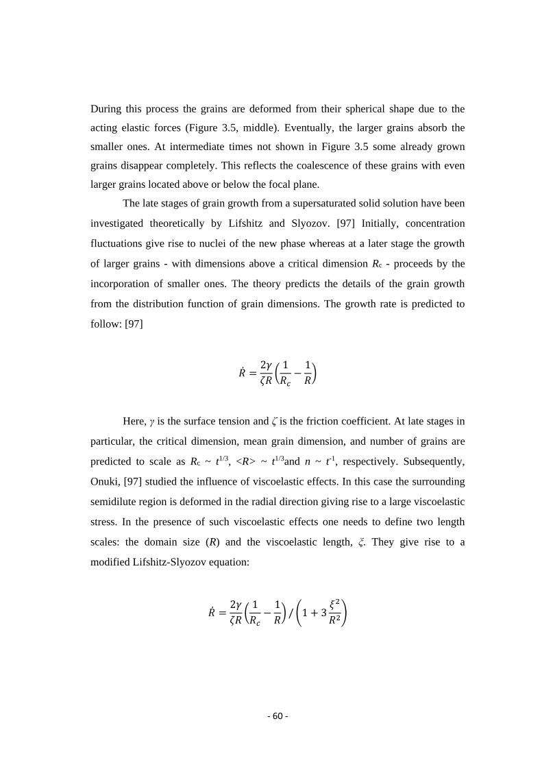
The late stages of grain growth from a supersaturated solid solution have been
investigated theoretically by Lifshitz and Slyozov. [97] Initially, concentration
fluctuations give rise to nuclei of the new phase whereas at a later stage the growth
of larger grains - with dimensions above a critical dimension Rc - proceeds by the
incorporation of smaller ones. The theory predicts the details of the grain growth
from the distribution function of grain dimensions. The growth rate is predicted to
follow: [97]
�̇� =2𝛾
𝜁𝑅(
1
𝑅𝑐−
1
𝑅)
Here, γ is the surface tension and ζ is the friction coefficient. At late stages in
particular, the critical dimension, mean grain dimension, and number of grains are
predicted to scale as Rc ~ t1/3, <R> ~ t1/3and n ~ t-1, respectively. Subsequently,
Onuki, [97] studied the influence of viscoelastic effects. In this case the surrounding
semidilute region is deformed in the radial direction giving rise to a large viscoelastic
stress. In the presence of such viscoelastic effects one needs to define two length
scales: the domain size (R) and the viscoelastic length, ξ. They give rise to a
modified Lifshitz-Slyozov equation:
�̇� =2𝛾
𝜁𝑅(
1
𝑅𝑐−
1
𝑅) / (1 + 3
𝜉2
𝑅2)

- 61 -
where ξ = (4η/3ζ)1/2 and η the zero shear viscosity. In polymer blends, ξ cannot
exceed the tube length, hence R >> ξ and eq. 1 is valid for large droplets.
Herein using the results of the in situ monitoring we plot the mean grain
dimension (<2R>) and number of grains (n) for the PS116/PMPS16 blend during
annealing at 120oC in Figure 3.6. For the shorter times, both n(t) and <R>(t) deviate
from the predictions for late stage SD. This suggests that at t <103 s, the blend is in
the elastic regime where the domain shape is determined by a balance between the
elastic forces and the interfacial tension. [98] Within this regime the composition of
each phase changes with time by the diffusion of PS from the PMPS-rich phase to
the PS-rich phase. Furthermore the area fraction of the less viscoelastic phase
(PMPS-rich) is about 0.3, i.e. much below the PMPS blend composition. The low
fraction is in agreement with the results from the earlier DS investigation that
identified a substantial PMPS fraction within the PS-rich phase. [81]
Figure 3.6. Evolution of the number of grains (top) and mean grain dimensions
(bottom) for the PS116/PMPS16 blend at 120oC. The vertical arrows indicate the
times where grains move out of the focal plane and coalesce with larger grains.
This affects both their number and average grain dimension. Lines with slopes of
1 (top) and 0.33 (bottom) are shown.

- 62 -
3.5. Purity of domains
The LSCM images shown above do not have enough contrast to account for
small amounts of fluorescently labeled PS that may be present within the PMPS
phase. Bellow we will show that the technique of FCS when coupled with LSCM can
provide additional information on the purity of phases in individual domains with
sub-micrometer special resolution.
As discussed in details in Chapter 2, FCS is based on monitoring and
recording the fluorescent intensity fluctuations caused by the diffusion of single
fluorescent species through the focus of a confocal microscope. Autocorrelation
analysis of these fluctuations yields the diffusion coefficient of the species. To enable
FCS, small amount of the fluorescent dye TDI was introduced as tracers in the
PS116/PMPS16 blend. It should be stressed that the absorption maximum of TDI is
around 630 nm i.e. far away from that of fluorescein (~480 nm) used for labeling the
PS phase. Thus, the two dyes can be excited individually by different lasers and their
fluorescence can be detected also individually. The procedure was as follows: prior
to the FCS measurement, LSCM images were recorded using excitation at 488 nm
(for fluorescein labeled PS) and then the laser focus was pointed in the center of a
chosen PMPS domain and the excitation wavelength changed to 633 nm (for the
TDI). (Figure 3.7)

- 63 -
The time-dependent fluctuations of the fluorescent intensity caused by the
diffusion of the TDI tracers through the focus were recorded and the corresponding
autocorrelation curves yield the tracer diffusion time and diffusion coefficient.
Subsequently, a new position was chosen within the PMPS-rich domain by moving
the focus by 1 μm away from the center and the auto-correlation curve was obtained
(Figure 3.8b)
This procedure was repeated at 1 μm increments from the center of the
domain up to the domain boundaries. Measurements were performed in domains
with different sizes from 3 to 20 microns.
Laser
Objective
Detector
Figure 3.7. Sketch illustrating the performance of FCS measurements in PMPS
domain of the phase separated polymer blend.

- 64 -
Typical results of the FCS measurements for the PS116/PMPS16 blend first
annealed at 120oC for 24 h and subsequently quenched at ambient temperature and
measured after a period of ~2 h are shown in Figure 3.8a.
Figure 3.8. (a) Normalized autocorrelation curves of terylene dye diffusing in
bulk PMPS () and within the PMPS domain (▲) of the PS116/PMPS16 blend. (b)
Diffusion times of terylene dye as a function of measuring position within the
PMPS-rich domain of the LSCM image (). The diffusion time of the same dye
in bulk PMPS () at the same temperature is also shown for comparison. The line
is a guide to the eye.
(a)
(b)

- 65 -
The Figure depicts normalized autocorrelation curves of TDI corresponding
at position 2 of the LSCM image.
For comparison, the autocorrelation curve for the diffusion of the same dye in
a PMPS homopolymer at ambient temperature is also shown. The figure further
compares the diffusion times as a function of the measuring position within the
PMPS grain. We can deduce that the TDI tracer is diffusing freely (according to the
Fick’s law) with nearly identical diffusion times in all cases.
Thus, the results shown in Figure 3.8 indicate that the large dark domains are
composed nearly exclusively by PMPS chains. This finding may sound paradoxical
since it is the experience with polymer blends that one of the coexisting phase
contain at least some amounts of the counter component. However, a closer
inspection of the PS/PMPS phase diagram (Figure 3.1) reveals that at ambient
temperature the PMPS phase is exclusively composed from PMPS chains.
To explore further this point a strongly asymmetric PS116/PMPS16 blend was
prepared (2/98) with the outlined procedure and imaged with LSCM. In Even at this
composition phase separated PS domains were clearly observed (Figure 3.9) in
accord with the phase diagram. In addition, the result is in excellent agreement with
the local segmental relaxation of PMPS in the PS48/PMPS17 symmetric blend
investigated earlier with dielectric spectroscopy. [21]
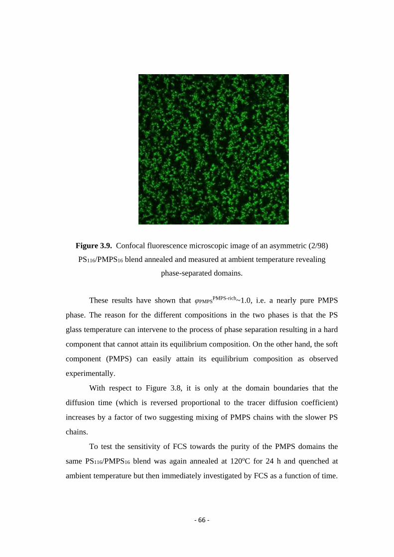
- 66 -
These results have shown that φPMPSPMPS-rich~1.0, i.e. a nearly pure PMPS
phase. The reason for the different compositions in the two phases is that the PS
glass temperature can intervene to the process of phase separation resulting in a hard
component that cannot attain its equilibrium composition. On the other hand, the soft
component (PMPS) can easily attain its equilibrium composition as observed
experimentally.
With respect to Figure 3.8, it is only at the domain boundaries that the
diffusion time (which is reversed proportional to the tracer diffusion coefficient)
increases by a factor of two suggesting mixing of PMPS chains with the slower PS
chains.
To test the sensitivity of FCS towards the purity of the PMPS domains the
same PS116/PMPS16 blend was again annealed at 120oC for 24 h and quenched at
ambient temperature but then immediately investigated by FCS as a function of time.
Figure 3.9. Confocal fluorescence microscopic image of an asymmetric (2/98)
PS116/PMPS16 blend annealed and measured at ambient temperature revealing
phase-separated domains.

- 67 -
Under such conditions the PMPS-rich phase may contain some slower PS chains. All
measurements were made at the center of the domain and the result is shown in
Figure 3.10, which depicts the diffusion time of TDI in the center of the PMPS reach
domain as a function of the time after quenching from 120°C to room temperature. In
the beginning the dye diffuses much slower than in pure bulk PMPS, indicating the
presence of remaining PS chains.
Figure 3.10. (Top) Normalized autocorrelation curves of TDT diffusing within
the PMPS domain directly after quenching from 120oC to room temperature
(filled circles) and in the same PMPS domain after 3 hours (filled squares) of the
PS116/PMPS16 blend. Measurements were made in the center of the domain.
(Bottom) Diffusion times of TDI as a function of measuring time within the
center of the PMPS-rich domain of the LSCM image.

- 68 -
Later these chains leave the domain and the diffusion time of TDI reaches a constant
value similar to that measured in pure PMPS. Thus, FCS is able to track in a unique
way the late stages of the phase separation inside micron-sized domains.
3.6. Conclusion
The in situ investigation of the phase separation by LSCM was coupled with
ex situ FCS measurements that provided both the dynamics of phase demixing and
the purity of phases in a symmetric polymer blend. This combination demonstrated
the possibility to obtain independent microscopic information on the local
concentration within the phase-separated domains and further allowed estimating the
interfacial width of a phase-separated blend by dynamic means. It would be of
interest to explore the purity of phases for other blend compositions or in other blend
systems that how bicontinuous phases instead.

- 69 -
CHAPTER 4
Dynamics in glassy
solutions of star shaped polymers
4.1. Introduction and motivation
In the past twenty years soft matter has become a field of growing interest.
[99] First reason is that soft matter is in our everyday life (blood, clay, plastics,
DNA, proteins, etc.). Another one is soft matter has by now reached even
technological relevance, for example in biotechnological or pharmaceutical
applications. [100] Among the systems comprised in soft matter (liquids, gels, foams,
polymers, granular materials, etc.), colloidal suspensions represent a large and
prominent field.
Since years it’s known that by increasing the volume fraction, colloidal
suspensions reach a frozen state. In a hard sphere suspensions, when the volume
fraction exceeds the value of 0.58 any of the given particles is surrounded with up to
12 neighboring particles and this restrict macroscopic motion, and thus the whole
suspension undergoes transition to a dynamically arrested state, which is glass. [101]
The glass formation is discussed in the context of caging (Figure 4.1), [102] particles
remain trapped in cages and there is only in-cage motion present, which constitute
the -relaxation process. After some time particle escapes from the cage, which leads
to terminal relaxation; this process is called -relaxation. In order to describe glassy
dynamics in hard spheres, especially in the linear response regime, various versions
of the mode-coupling theory (MCT) were provided. [103, 104]

- 70 -
Another attractive system is soft colloidal suspensions; such are for example
multiarm star shaped polymers, which consist of f chains chemically anchored on a
common center. By variation of functionality f one can control the softness of the
colloids. (Figure 4.2 image taken from [105]) The glass formation of soft star
polymers can also be formulated in context of caging. However in comparison to
hard spheres there interaction is softer, and being deformable, stars can interpenetrate
at higher concentrations. The polymeric nature of stars adds some interesting
features. Due to their partial interpenetration, the outer blobs of the neighboring
caged particles form effective entanglements, and therefore -relaxation proceeds
through both factors: disengagement of the stars from neighbors and cage opening
like in case of hard sphere colloidal glasses.
Although these materials macroscopically behave like a glass, even at
relatively low polymer concentration, at nanoscopic level the mobility is still present.
[105, 106]
The aim of this project was to investigate the dynamics in these soft colloidal
systems. By probing the tracer diffusion at microscopic level using FCS we can
study, whether tracer and solvent molecules mobility in present system is affected by
Figure 4.1. Cartoon representing caging for hard spheres.

- 71 -
this macroscopical “glass transition”. Additional information how the tracer
dynamics can be affected by the glass transition is given in this paper. [24]
4.2. Materials and sample.
In order to study the dynamic in soft colloidal systems we used the specific
star shaped polymers provided by the group of Dimitris Vlassopoulos. [105] They
consist of a hard dendritic core and a soft polybutadiene outer shell. Each carbosilane
dendritic core comprises 128 Si–Cl functional groups, which were first coupled to
1,2-poly(butadienyl)lithium chains with numberand weight-average molar masses
Mn = 1.20 kg mol-1 and Mw = 1.32 kg mol-1, respectively. The hydrodynamic radius
of the colloidal stars in very dilute solutions was measured by DLS: Rh = 40 nm at T
= 20 0C. The corresponding overlapp concentration was calculated and found to be
Ch* = 57 mg ml-1. The detailed information of the syntheses of these colloidal stars
can be found in following paper. [105]
Figure 4.2. Cartoon illustration of interpenetrating stars in
solution.
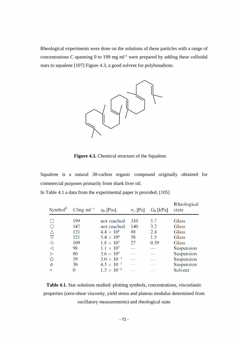
- 72 -
Rheological experiments were done on the solutions of these particles with a range of
concentrations C spanning 0 to 199 mg ml-1 were prepared by adding these colloidal
stars to squalene [107] Figure 4.3, a good solvent for polybutadiene.
Squalene is a natural 30-carbon organic compound originally obtained for
commercial purposes primarily from shark liver oil.
In Table 4.1 a data from the experimental paper is provided. [105]
Figure 4.3. Chemical structure of the Squalene
Table 4.1. Star solutions studied: plotting symbols, concentrations, viscoelastic
properties (zero-shear viscosity, yield stress and plateau modulus determined from
oscillatory measurements) and rheological state

- 73 -
In order to prepare the concentrated solutions for FCS measurements,
tetrahydrofuran (THF) was added in excess as a co-solvent in order to promote
dispersion and mixing of the stars. Under continuous mixing the THF was
evaporated away with vacuum applied as a finishing step to assist in the full removal
of the co-solvent. In addition TDI was added with concentration 10-9 g mol-1
4.3. Tracer diffusion in star shaped polymer solutions
Star shaped polymer solutions in squalene were prepared with concentrations
ranging from 10-50 weight %. Solution was putted on the microscope glass slide,
was fixed in attofluor chamber (Figure 4.4), and mounted on the microscope.
The FCS measurement was performed in the middle of the “glassy” polymer above
the glass surface. The example of autocorrelation curves of TDI dye in the “glassy”
polymers at different concentration is given in Figure 4.5.
Figure 4.4. Cartoon illustrating how the sample was prepared for FCS
measurements

- 74 -
0.01 0.1 1 10 100 1000
0.0
0.2
0.4
0.6
0.8
1.0
1.2(G
(t)
-1)/
(G (
0)-
1)
Time (ms)
TDI in Toluene
TDI in Squalene
First TDI was measured in pure squalene, and after that the concentration of
the polymer was set to 10 weight%, next step the concentration of the polymer was
further increased till 20% and so by step of 10% till 50%. Curve of TDI diffusing in
bulk toluene is given for a comparison. To be sure in the reproducibility of the
results, measurements were performed several times at different position through the
thickness of the glassy polymer film. All the autocorrelation curves were fitted with
the single component diffusion model.
From Table 4.1 we can see that the that the rheological state of the polymer solution
changes from “suspension” to glass when we go from concentration 98 g ml-1 to 109
g ml-1. If we recalculate the concentration, in our case this jump should appear at
C o n c e n t r a t i o n
Figure 4.5. Normalized autocorrelation functions obtained for TDI diffusing in
bulk toluene, bulk squalene and in “glassy” polymer solutions, by increasing the
weight % of the polymer by 10% each step.

- 75 -
concentration about 30%. However as can be seen from the Figure 4.6, the TDI
diffusion time increases monotonically with the increase of the star polymer
concentration over the entire studied range and nothing peculiar happens and the
concentration of “glass transition”. Thus, we see that the small molecule still “freely”
diffuses in the polymer solution, even though macroscopically the solution is in
glassy state.
0 10 20 30 40 50
0.0
0.5
1.0
1.5
2.0
2.5
3.0
3.5
4.0
Diffu
sio
n t
ime [
ms]
~ 1
/diffu
sio
n c
oef.
concentration w.%
glasssuspension
This can be explained by the formation of the channels between the polymeric
“stars”, which due to their size cannot come close to each other. There is some space
Figure 4.6. Striking difference between macroscopic an microscopic properties:
the macroviscosity increase strongly with concentration and above~30% glassy
behavior and in contrast the small tracer diffusion decrease only slightly and
continuously with concentration

- 76 -
left in between the “stars”, which is more than enough for the small molecule like
TDI to diffuse without restriction.
In Figure 4.7 we have plotted the normalized TDI diffusion coefficient (on
the value measured in pure squalene) vs. the star shape polymer concentration in
order to compare our results with existing data for the diffusion of various small
tracers in solutions of linear polymers that have been shown to fall on a single
“master curve”. The plotted master curve presents reported diffusion coefficients for
polymer systems obtained by measuring by different experimental techniques [108]
Meerwall et al. [109] studied the diffusion of hexafluorobenzene in PS (10k to
1000k)/THF solutions by pulsed field gradient spin-echo NMR. Chekal and
Torkelson [110] reported behavior of a styrene monomer diffusing in polystyrene
solutions down to a matrix PS molecular weight Mw of 1300 g/mol. More recently
diffusion of a small PMI dye in polymer solution studied by FCS was reported. [23]
All the presented data from the literature indicate that the polymeric nature of the
matrix expressed by its molecular weight or that is the same by its crossover
concentration does not affect the small probe behavior. Instead it is only the
crowding effect of the environment molecules that reduces the diffusion rate of the
small probes in such solution.

- 77 -
Figure 4.7. Normalized diffusion coefficients of various small tracers. Green
rhombs represent the data for the TDI in star polymer/squalene solutions.
From my studies which, correspond to green rhombs on the plot Figure 4.7
we can see that tracer slowdown is even smaller in the present system of star shaped
polymers as compared to the linear polymer solutions. This can be considered as
afurther evidence that the channel can form between the polymeric stars and
facilitate the diffusion.
In order to address the size dependent diffusion in “glassy” polymer solution,
I decided to study the diffusion of the bigger fluorescent tracers. Qdots which have
size in radius of about 5nm and the excitation maximum 633nm were used. Before
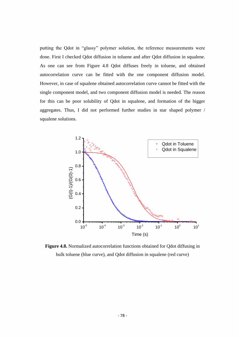
- 78 -
putting the Qdot in “glassy” polymer solution, the reference measurements were
done. First I checked Qdot diffusion in toluene and after Qdot diffusion in squalene.
As one can see from Figure 4.8 Qdot diffuses freely in toluene, and obtained
autocorrelation curve can be fitted with the one component diffusion model.
However, in case of squalene obtained autocorrelation curve cannot be fitted with the
single component model, and two component diffusion model is needed. The reason
for this can be poor solubility of Qdot in squalene, and formation of the bigger
aggregates. Thus, I did not performed further studies in star shaped polymer /
squalene solutions.
10-5
10-4
10-3
10-2
10-1
100
101
0.0
0.2
0.4
0.6
0.8
1.0
1.2
(G(t
)-1)/
(G(0
)-1)
Time (s)
Qdot in Toluene
Qdot in Squalene
Figure 4.8. Normalized autocorrelation functions obtained for Qdot diffusing in
bulk toluene (blue curve), and Qdot diffusion in squalene (red curve)

- 79 -
4.4. Conclusion
Diffusion of the small fluorescent dye TDI was studied using Fluorescence
Correlation Spectroscopy in star shaped polymer solutions, at different dilutions.
FCS measurements showed that even though the polymer solution above the
concentration of 30 weight % macroscopically has properties of “glass” the
microscopically the tracer mobility is still present and not affected by the transition
to the glassy state. The small dye can “freely” diffuse in a “glassy” polymer solution
through the microscopic channels that form between the dendritic stars. In order to
address the size dependent diffusion, a bigger fluorescent dye namely Qdot with the
radius of 5.5 nm was also studied in the system, however due to the aggregate
formation in the solvent squalene could not give reliable results. Further studies with
other tracers and with fluorescently labeled stars are currently underway.

- 80 -

- 81 -
CHAPTER 5
Temperature controlled diffusion in
PNIPAM modified Silica Inverse Opals
5.1. Introduction and motivation
Understanding and controlling the diffusion of small molecules,
macromolecules and nanoparticles in complex, nanostructured environments is of
paramount fundamental and technological importance. A number of theories and
models have been introduced to describe the diffusion of small species in polymer
systems, in intercellular matrices or in solid periodic nano-porous structures.
From applications point of view, the possibility for on demand control of the
diffusion of small penetrants in nanoporous structures is even more important.
Indeed, such possibility gives various opportunities as to e.g. control the drug release
rate or to select the relevant sizes in a separation process. Traditionally, control over
the penetrant diffusion is achieved by changing the size and/or density of the
nanopores. However, in a solid nanoporous structure, such as, an anodized aluminum
membrane, a porous glass or a silica inverse opal, the pore size is determined during
the fabrication process and typically cannot be changed e.g. by applying an external
stimulus. This is unfortunate, because on the other hand the solid nanoporous
structures offer the mechanical strength and stability that is required for most
applications. Alternatively, in some polymer based nanoporous systems such as e.g.
hydrogels, the pore size and thus the penetrant diffusivity can be controlled by tuning
the temperature or the pH value. Hydrogels, however, lack mechanical stability that
often makes their application problematic.

- 82 -
In this project, I will describe a new system combining the mechanical
stability of a solid nanoporous structure with the possibility for fine tuning offered by
a thermo responsive polymer. As a solid support I used a silica inverse opal (iOpal),
which is a highly order porous structure, consisting of regular arrangements of
spherical voids surrounded by solid silica walls with interconnecting circular
pores.[111-114] Due to their well-defined nanoporous structure iOpals have been
often used as model systems to study the diffusion of small molecules [24],
nanoparticles or DNA. [115] Here, I modified the iOpal interior surface with grafted
Poly(N-isopropylacrylamide) (PNIPAM) brushes. The PNIPAM is one of the most
popular thermo responsive polymers and exhibits a lower critical solution
temperature (LCST) of around 32oC [116] i.e. close to the humans body temperature.
In aqueous solutions, below the LCST the PNIPAM chains are hydrated and adopt an
extended coil conformation, while above the LCST they are dehydrated and collapse
to a globular conformation. Correspondingly, the PNIPAM brushes grafted to the
iOpal interior surface will swell under the LCST decreasing the overall porosity of
the system and shrink above the LCST increasing the porosity (Figure 1). This offers
the possibility for a temperature control over the diffusivity of small penetrants
inside the iOpal.
PNIPAM, grafted on porous silica nanoparticles [117] or porous silicon
films[118] was used previously for temperature controlled entrapping and release of
model drug molecules. Here, I go a step further and focus on direct monitoring of the
penetrants mobility inside the PNIPAM modified iOpals. For this purpose I used
fluorescence correlation spectroscopy (FCS) (Detailed description of FCS Chapter 1)
as it has very small probing volume (< 1 µm3) that can be easily positioned on
various places in the studied nanoporous structure and thus provide local information
on the penetrant mobility.

- 83 -
5.2. Materials and sample preparation
5.2.1. Silica Inverse Opals
5.2.1.1. Preparation via Vertical Deposition method
Initially Silica inverse opals (iOpals) were fabricated using Vertical
Deposition (VD) method (Detailed description in Chapter 1) Monodisperse PS
colloids of 100-1000 nm and 7nm silica nanoparticles were co-deposited from
aqueous suspension on round microscope glass slides (Menzel, Germany) with
diameter and thickness of 25 mm and 0.17 mm respectively. Procedure is illustrated
in Figure 5.1.
Figure 5.1. Preparation of colloidal crystal in humidity chamber via VD
deposition method. White Teflon vessel is filled with the mixture of Polystyrene
and SiO2 nanoparticles. The microscope cover glasses are covered from one side
with the blue polyethylene films to avoid the crystal formation on this side.

- 84 -
Prior deposition, glass slides were cleaned by a 2% Hellmanex solution
(Hellma, Germany) and hydrophilized by a plasma treatment. In addition in order to
have a formation of the opal only on the one side of the glass, the other side was
covered with the commercially available polyethylene film.
VD was performed in a temperature range 20-25oC and humidity 30-80%, in
a special humidity chamber with the lifting speed from 200 nm/s to 800 nm/s.
Concentration range of PS colloids was 0.5 – 4 wt%, whereas SiO2 particle
concentration was kept constant 0.3 wt%.
Inversed SiO2 opals were obtained after removal of the PS spheres by
calcination at 500 °C for 5 h. (Figure 5.2.)
The quality and size of the dry inverse opals were characterized by scanning electron
microscope (SEM) Figure 5.3. From the SEM images we can see, that opals have
voids with the size comparable to the PS particle size from which they were
fabricated. And these voids are connected to each other with the holes.
Figure 5.2. Removing polystyrene template via calcination at 500oC, after 5 hours
the well order structure of SiO2 is left.

- 85 -
(d)
Figure 5.3. Scanning electron microscopy images of inverse opals made from (a)
100nm, (b) 200 nm, (c) 300 nm and (d) 1000 nm polystyrene particles.
(c)
(d)
(b)
(a)

- 86 -
5.2.1.2. Modification via ATRP
Silica Inverse Opals with a void diameter 300 nm (Figure 5.4c) were
modified with thermoresponsive polymer brushes via Atom transfer radical
polymerization (ATRP) method (Detailed description in Chapter 1). Gel Permeation
Chromatography (GPC) method was used to determine molecular weight of the
polymer obtained from bulk polymerization.
5.2.1.2.1 Materials
N-Isopropylacrylamide (NIPAM), CuBr, Ethyl 2-bromoisobutyrate were
purchased from Aldrich. 1,1,4,7,7-Pentamethyldiethylenetriamine (PMDETA) was
purchased from Acros. The starter 3-(2-bromoisobutyryl)propyl)dimethyl
chlorosilane was synthesized following the procedure described in the literature.
[119] NIPAM monomer was recrystallized from hexane. CuBr was purified by
boiling in mixture of 1:1 (by volume) Millipore water/ acid acetic and subsequently
filtered off. The precipitate was rinsed with water, ethanol, and finally with diethyl
ether and dried in a vacuum oven for 24 h. (2-EiBBr) (Aldrich, 98%) was used
without further cleaning. Toluene was distilled from sodium under Argon
atmosphere. Triethylamine was distilled from CaH2 and stored under Argon
atmosphere. All aqueous solutions were prepared with ultrapure water purified with a
Milli-Q UV-Plus water purification system (Millipore, Bedford, MA). The water had
a resistivity of >18Mcm-1.
5.2.1.2.2 Initiator Immobilization
In order to prepare the silicon surface for the starter immobilization and to
assure controlled hydration state of the silicon oxide layer on top, a base cleaning
was performed. Silica inverse opal was immersed in a mixture of NH3 (4 mL, 25%),
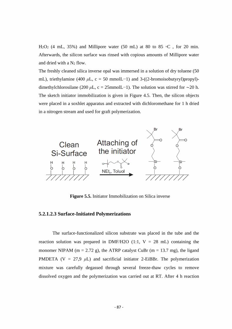
- 87 -
H2O2 (4 mL, 35%) and Millipore water (50 mL) at 80 to 85 ◦C , for 20 min.
Afterwards, the silicon surface was rinsed with copious amounts of Millipore water
and dried with a N2 flow.
The freshly cleaned silica inverse opal was immersed in a solution of dry toluene (50
mL), triethylamine (400 μL, c = 50 mmolL−1) and 3-((2-bromoisobutyryl)propyl)-
dimethylchlorosilane (200 μL, c = 25mmolL−1). The solution was stirred for ∼20 h.
The sketch initiator immobilization is given in Figure 4.5. Then, the silicon objects
were placed in a soxhlet apparatus and extracted with dichloromethane for 1 h dried
in a nitrogen stream and used for graft polymerization.
5.2.1.2.3 Surface-Initiated Polymerizations
The surface-functionalized silicon substrate was placed in the tube and the
reaction solution was prepared in DMF/H2O (1:1, V = 28 mL) containing the
monomer NIPAM (m = 2.72 g), the ATRP catalyst CuBr (m = 13.7 mg), the ligand
PMDETA (V = 27,9 μL) and sacrificial initiator 2-EiBBr. The polymerization
mixture was carefully degassed through several freeze-thaw cycles to remove
dissolved oxygen and the polymerization was carried out at RT. After 4 h reaction
Figure 5.5. Initiator Immobilization on Silica inverse
opals

- 88 -
time the silica inverse opal was removed from the polymerization mixture rinsed
with dichloromethane and dried.
Subsequently, they were placed in a Soxhlet apparatus, continuously extracted with
toluene for 18 h, and dried. The polymer generated in solution with the initiator
added sacrificially was recovered by precipitating the reaction mixture into methanol,
filtering and drying in vacuum. For gel-permeation chromatography (GPC) analysis
(Figure 4.6) solutions of the polymers were briefly filtered over alumina to remove
residual copper complex.
From GPC analyses polymer has a molecular weight of 25K and
polydispersity D=1.37 Modified Silica Inverse Opals were also analyses with SEM
and compared to not modified one (Figure 4.7). From the images one can see the
presence of the polymer layer grafted from voids of the Silica Inverse Opal modified
with PNIPAM brushes.
Figure 5.6. Gel-permeation chromatography of the polymer generated in the
solution.

- 89 -
5.3. Tracer diffusion in PNIPAM modified iOpals
We used FCS to study the effect of the grafted PNIPAM brushes on the
diffusion of the small molecular dye Alexa Fluor 647 in the modified iOpals. Figure
5.8 shows a typical FCS autocorrelation curve measured in the middle of an iOpal
modified with PNIPAM with Mw=25224. For comparison the autocorrelation curve
measured in an iOpal modified only with very short PNIPAM chains (Mw=4981) is
also shown. This sample was used as a reference instead of a completely unmodified
opal in order to account for the different surface chemistry of the later that may
induce adsorption of the tracers on the bare silica surface. [120] From Figure 5.8 it is
obvious that the autocorrelation curve measured in the iOpal modified with long
PNIPAM chains is strongly shifted to the longer lag times, reflecting significantly
slower diffusion. Both curves can be nicely fitted using single component diffusion
model (details Chapter 1) yielding diffusion times of d=1200 s and d =140 s in
the iOpals modified with long and short PNIPAM brushes respectively. For
comparison the diffusion of the same tracer in pure water is even faster (Figure 5.8)
with diffusion time d=42 s. In our experiment, the objective’s immersion medium
Figure 5.7. Scanning electron microscopy images of Silica inverse opal (a,b,c)
and Silica inverse opal modified with PNIPAM Brushes (d).
(f)

- 90 -
was water with refractive index n ≈ 1.33. For the water-filled PNIPAM modified
inverse opal with silica (n ≈ 1.45) and filling volume fraction of about 20%, the
effective refractive index was n ≈ 1.36. Due to this small refractive index mismatch,
the estimated error of the diffusion coefficient in the inverse opals was less than
10%.[121-123] Thus the strong shift of the autocorrelation curves for the inverse
opals toward to longer times (Figure 5.8) was caused by the confinement, as
discussed and theoretically rationalized before.[123]
1E-5 1E-4 1E-3 0.01 0.1
0.0
0.2
0.4
0.6
0.8
1.0
1.2
In Bulk water
In iOpal (short PNIPAM)
In PNIPAM modified iOpal
(G (
t)-1
)/G
(0)-
1)
Time (s)
In order to verify the reproducibility of these results, FCS measurements were
performed at various lateral positions in the studied iOpals. These measurements
Figure 5.8. Normalized autocorrelation functions obtained for Alexa Fluor 647
diffusing in bulk
and in PNIPAM modified Silica Inverse opal (O). The solid lines represent the
corresponding fits.
(g)

- 91 -
yielded very similar results. The situation changes qualitatively, however, when the
FCS measurements were performed at different axial positions through the thickness
of the iOpals. As shown in Figure 5.9, Alexa Fluor 647 molecules diffuse faster in
bottom layers of the inverse opal (d =590 μs) in comparison to upper layers of the
inverse opals (d=590-1200 μs). This indicates that the molecular weight of the
grafted PNIPAM is different in different layers. Such finding is not surprising
tacking into account that the iOpal film is formed on a glass substrate (Figure 5.3c)
and thus opened to the environment only from its upper side. During the ATRP
process monomers have to diffuse through the entire iOpal film thickness in order to
reach the bottom layer.
10-5
10-4
10-3
10-2
10-1
100
0.0
0.2
0.4
0.6
0.8
1.0
1.2
(G (
t)-1
)/G
(0)-
1)
Time (s)
3 microns from surface
5 microns from surface
8 microns from surface
Figure 5.9. Cartoon representing the tracer diffusion in PNIPAM modified
inverse opal at different distance from glass slide.

- 92 -
Thus the PNIPAM brushes grow faster in the upper than in the lower layers
of the iOpal forming a gradient of the final brush length in the axial direction. It is
important to emphasize that due to the extremely small probing volume of the FCS
(~1 µm in axial direction) the small fluorescent tracer diffusion studies can nicely
capture this gradient in film as thin as few micrometers only.
5.4. Temperature dependent diffusion
Now I focus on the possibility to tune the diffusivity in the PNIPAM
modified iOpals by controlling the temperature and thus the PNIPAM brushes
conformation and in turn the overall nano-porosity of the systems. In order to
demonstrate this possibility I used FCS to study the diffusion of Alexa 647 molecules
in water filled PNIPAM modified iOpal at various temperatures in the range 20°C –
35°C i.e. below and above the lower critical solution temperature of PNIPAM. For
each measurement the system was kept at a constant temperature using a heating
stage. The autocorrelation curves were recorded in the upper layer of the PNIPAM
modified iOpal film (8 microns above the glass surface) where the length of the
grafted PNIPAM brushes was maximal. Typical autocorrelation curves measured at
temperatures of 20°C and 35°C are shown in Figure 5.10.
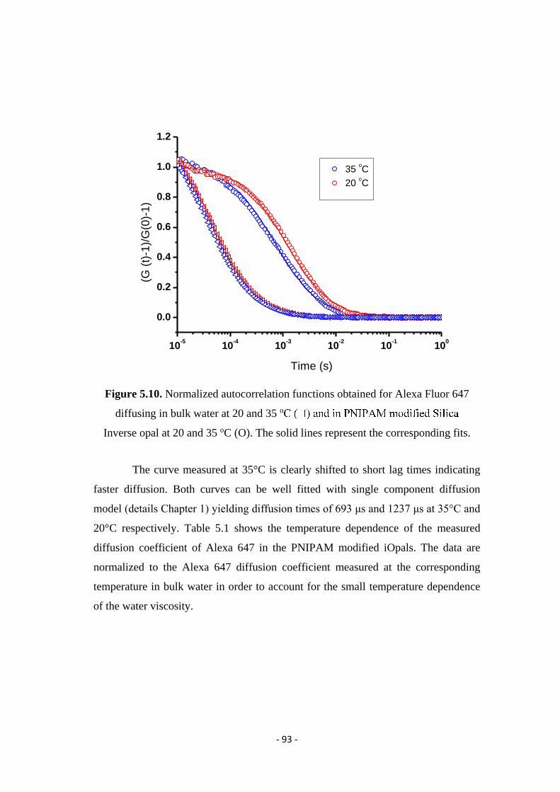
- 93 -
10-5
10-4
10-3
10-2
10-1
100
0.0
0.2
0.4
0.6
0.8
1.0
1.2(G
(t)
-1)/
G(0
)-1)
Time (s)
35 oC
20 oC
The curve measured at 35°C is clearly shifted to short lag times indicating
faster diffusion. Both curves can be well fitted with single component diffusion
model (details Chapter 1) yielding diffusion times of 693 μs and 1237 μs at 35°C and
20°C respectively. Table 5.1 shows the temperature dependence of the measured
diffusion coefficient of Alexa 647 in the PNIPAM modified iOpals. The data are
normalized to the Alexa 647 diffusion coefficient measured at the corresponding
temperature in bulk water in order to account for the small temperature dependence
of the water viscosity.
Figure 5.10. Normalized autocorrelation functions obtained for Alexa Fluor 647
diffusing in bulk water at 20 and 35 o
Inverse opal at 20 and 35 oC (O). The solid lines represent the corresponding fits.

- 94 -
Temperature (oC) Alexa 647 in bulk water Alexa 647 in PNIPAM iOpal
20 44 1237
25 42 1170
30 40 1012
35 38 693
The data clearly demonstrate a temperature induced speed-up of the penetrant
mobility in PNIPAM modified silica inverse opal caused by the stretching and
collapsing of polymer brushed inside the iOpal as shown in Figure 5.11. Moreover
this change in mobility is fully reversible as confirmed by repeating the
measurements after several heating and cooling cycles.
Figure 5.11. Cartoon representing the opening and closing mechanism in
PNIPAM modified inverse opal at different temperatures.
Table 5.1. Diffusion time versus temperature of Alexa Flour 647 in bulk water
and in PNIPAM modified Silica Inverse Opal.

- 95 -
5.5. Conclusion
Silica inverse Opals were modified with the termoresponsive polymer brushes
via Atom transfer radical polymerization (ATRP) method and the effect of molecular
crowding was investigated by Fluorescence correlation Spectroscopy. The presented
results demonstrated that the dynamics in Silica Inverse Opals grafted with
temperature responsive polymers brushed is becoming significantly slower. And by
opening and closing interconnecting holes of the silica inverse opals, via stretching
and collapsing polymer brushes the dynamics of the molecular and macromolecular
tracers can be controlled.

- 96 -

- 97 -
CHAPTER 6
Summary and conclusions
Fluorescence correlation spectroscopy (FCS) is a prominent technique to
investigate the diffusion of fluorescence species in various surroundings. The method
is based on the measurement of the fluorescence intensity fluctuations caused by
fluorescence species diffusing through a small observation volume (V < 1μm3) of a
confocal microscope. This allows FCS to address the diffusion of fluorescence
species at extremely low concentration (nM), and provides a great potential to locally
access systems that require high spatial resolution. Until very recently, however, FCS
has been applied mainly to biological, i.e. aqueous environments.
In this thesis I used FCS to study tracer diffusion in heterogeneous systems of
synthetic nature. In the first part of my thesis using the combination of the laser
scanning confocal microscopy (LSCM) and fluorescence correlation spectroscopy
(FCS) I studied in situ the dynamics of phase separation in the polymer blend
polystyrene/poly(methyl phenyl siloxane) (PS/PMPS) at the macroscopic and
microscopic length scales, respectively. LSCM was used to monitor the process of
phase separation in real time providing images of droplet coalescence and growth
during the intermediate and late stages. Measuring the small tracer (terrylene dye)
diffusion in the PMPS phase of the phase separated blend and by comparing the
diffusion of the same tracers in pure bulk PMPS, additional information on the purity
of phases was obtained using FCS.
In the second part of my thesis, FCS was utilized to investigate the diffusion
behavior of small fluorescent tracers in “glassy” polymer solutions. The polymers
used in these studies were colloidal stars consisting of a hard dendritic core and a soft
polybutadien outer shell. These polymers were dissolved in a solvent squalene and

- 98 -
above the concentration of ~30 weight % macroscopically has properties of a
“glass”, however by probing the tracer diffusion at microscopic level using FCS I
could show that the tracer and solvent molecules mobility in present system is not
affected by this macroscopical “glass transition”.
In the last part of my thesis I demonstrated a new stimuli responsive system
based on poly-N-isopropylacrylamide (PNIPAM) and silica inverse opals (iOpals),
which are known as a model of porous periodic nanostructures. The interior of the
iOpals was modified with PNIPAM brushes via grafting “from” approach using atom
transfer radical polymerization (ATRP) method. FCS in this case was applied to
study the effect of the temperature on the diffusion of molecular and macromolecular
tracers in the iOpal-PNIPAM system. The results, clearly demonstrate that the phase
transition of the temperature-responsive polymer can be used to control opening and
closing of the grafted iOpal pores and by that we can speed-up or slow-down the
mobility of the tracers.

- 99 -
Acknowledgements (are given in printed version)

- 100 -

- 101 -
List of symbols
C Concentration
c* Overlapping concentration
cp* Overlapping concentration of probe
D or Di Diffusion coefficient of species i
D0 Diffusion coefficient in pure solvent (at c = 0)
Ds Self diffusion coefficient
F(t’) Fluorescence intensity (kHz) at time t’
fi Fraction of species i
G(t) Autocorrelation function
G Gibbs free energy
λ Wavelength of light
λex Wavelength of excitation light
λem Wavelength of emission light
KB Bolzmann constant
Mn Number average molecular weight
Mw Weight average molecular weight
n Refractive index
N Number of monomers in polymer chain
NA Avogadro’s number
Np number of particles in the observation volume
<Δr²(t)> Mean square displacement
Rh Hydrodynamic radius
Rg Radius of gyration
r0 Radial axis of confocal volume
S Structure of parameter (= z0/r0)
t Experimental lag time
τD Lateral diffusion time

- 102 -
T Temperature
T0 Ideal glass transition temperature
Tg Glass transition temperature
V Observation volume
z0 Vertical axis of confocal volume
η Viscosity
ξ Polymer mesh size

- 103 -
List of abbreviations
ATRP Atom transfer radical polymerization
BP Band pass transmission filter
DLS dynamic light scattering
DS Dielectric spectroscopy
FCS Fluorescence correlation spectroscopy
FRAP Fluorescence recovery after photobleaching
FRS Forced Rayleigh scattering
GPC Gel Permeation Chromatography
iOpal Inverse Opal
LP Long pass transmission filter
LSCM Laser scanning confocal microscope
MSD Mean square displacement
NA Numerical aperture
NMR Nuclear magnetic resonance
PDI Perylene-diimide
PDMS Polydimethylsiloxane
PFG-NMR Pulsed-field-gradient NMR
PMI Perylene monoimide
PMT Photomultiplier
PMPS Poly(methyl phenyl siloxane)
PNIPAAm Poly (N-isopropylacrylamide)
PS Polystyrene
PSF Point Spread Function
Qdot Quantum dot
Rh6G Rhodamine 6G
SE Stokes-Einstein equation
SEM Scanning electron microscope
TDI Terrylene-diimide
THF Tetrahydrofuran
VD Vertical depostion

- 104 -
Publications (are given in printed version)
- 105 -
References
1. Fick, A., Annalen der Physik und Chemie, 94, 59 (1855). Uber Diffusion. 2. Einstein, A., Ist die Trägheit eines Körpers von seinem Energieinhalt abhängig?
Annalen der Physik, 1905. 323(13): p. 639-641. 3. Chandrasekhar, S. and M. Kac, Marian Smoluchowski: his life and scientific
work2000: Polish Scientific Publishers PWN Warsaw. 4. Von Smoluchowski, M., Zur kinetischen theorie der brownschen
molekularbewegung und der suspensionen. Annalen der Physik, 1906. 326(14): p. 756-780.
5. Hänggi, P., P. Talkner, and M. Borkovec, Reaction-rate theory: fifty years after Kramers. Reviews of Modern Physics, 1990. 62(2): p. 251.
6. Flynn, C.P. and J.J. Burton, Point defects and diffusion. Physics Today, 1973. 26: p. 61.
7. Berne, B.J., Dynamic light scattering: with applications to chemistry, biology and physics1976: DoverPublications. com.
8. Andrasko, J., Water diffusion permeability of human erythrocytes studied by a pulsed gradient NMR technique. Biochimica et Biophysica Acta (BBA)-General Subjects, 1976. 428(2): p. 304-311.
9. Déléze, J., et al., Fluorescence recovery after photobleaching, in Connexin Methods and Protocols2001, Springer. p. 313-327.
10. Lumma, D., et al., Dynamics of large semiflexible chains probed by fluorescence correlation spectroscopy. Physical Review Letters, 2003. 90(21): p. 218301.
11. DETECTION, S.M., Fluorescence Correlation Spectroscopy. Phys. Rev. Lett, 1972. 29: p. 705-708.
12. Rarbach, M., et al., Dual-color fluorescence cross-correlation spectroscopy for monitoring the kinetics of enzyme-catalyzed reactions. Methods, 2001. 24(2): p. 104-116.
13. Schwille, P., F. Oehlenschläger, and N.G. Walter, Quantitative hybridization kinetics of DNA probes to RNA in solution followed by diffusional fluorescence correlation analysis. Biochemistry, 1996. 35(31): p. 10182-10193.
14. Haustein, E. and P. Schwille, Ultrasensitive investigations of biological systems by fluorescence correlation spectroscopy. Methods, 2003. 29(2): p. 153-166.
15. Cluzel, P., M. Surette, and S. Leibler, An ultrasensitive bacterial motor revealed by monitoring signaling proteins in single cells. Science, 2000. 287(5458): p. 1652-1655.
16. Kim, B.-S., et al., Effect of organic solvent on the permeability and stiffness of polyelectrolyte multilayer microcapsules. Macromolecules, 2005. 38(12): p. 5214-5222.
17. Zhang, R., et al., Swelling of cross-linked polystyrene beads in toluene. Microelectronic Engineering, 2008. 85(5): p. 1261-1264.
18. Vagias, A., et al., Complex Tracer Diffusion Dynamics in Polymer Solutions. Physical Review Letters, 2013. 111(8): p. 088301.

- 106 -
19. Raccis, R., et al., Probing mobility and structural inhomogeneities in grafted hydrogel films by fluorescence correlation spectroscopy. Soft Matter, 2011. 7(15): p. 7042-7053.
20. Casoli, A. and M. Schönhoff, Fluorescence correlation spectroscopy as a tool to investigate single molecule probe dynamics in thin polymer films. Biological Chemistry, 2001. 382(3): p. 363-369.
21. Zettl, H., et al., Fluorescence correlation spectroscopy of single dye-labeled polymers in organic solvents. Macromolecules, 2004. 37(5): p. 1917-1920.
22. Grabowski, C.A. and A. Mukhopadhyay, Diffusion of polystyrene chains and fluorescent dye molecules in semidilute and concentrated polymer solutions. Macromolecules, 2008. 41(16): p. 6191-6194.
23. Cherdhirankorn, T., et al., Diffusion in polymer solutions studied by fluorescence correlation spectroscopy. The Journal of Physical Chemistry B, 2009. 113(11): p. 3355-3359.
24. Cherdhirankorn, T., et al., Fluorescence correlation spectroscopy study of molecular probe diffusion in polymer melts. Macromolecules, 2009. 42(13): p. 4858-4866.
25. Cherdhirankorn, T., et al., Effects of Chain Topology on the Tracer Diffusion in Star Polyisoprenes. Macromolecules, 2009. 42(22): p. 9183-9189.
26. Doroshenko, M., et al., Monitoring the Dynamics of Phase Separation in a Polymer Blend by Confocal Imaging and Fluorescence Correlation Spectroscopy. Macromolecular rapid communications, 2012. 33(18): p. 1568-1573.
27. Minsky, M., Memoir on inventing the confocal scanning microscope. Scanning, 1988. 10(4): p. 128-138.
28. Claxton, N.S., T.J. Fellers, and M.W. Davidson, Laser scanning confocal microscopy. Olympus. Available online at http://www. olympusconfocal. com/theory/LSCMIntro. pdf, 2006.
29. Melet, R., et al. Resonant emission of a single InAs/GaAs quantum dot in a waveguiding configuration. in AIP Conference Proceedings. 2007.
30. Pawley, J.B., Handbook of biological confocal microscopy1995: Springer. 31. Takeuchi, O., et al., Development of time-resolved scanning tunneling microscopy in
femtosecond range. Japanese journal of applied physics, 2002. 41(part 1): p. 4994-4997.
32. Webb, R.H., Confocal optical microscopy. Reports on Progress in Physics, 1996. 59(3): p. 427.
33. Lei, M. and B. Yao, Characteristics of beam profile of Gaussian beam passing through an axicon. Optics communications, 2004. 239(4): p. 367-372.
34. Pawley, J.B., Fundamental limits in confocal microscopy, in Handbook of biological confocal microscopy2006, Springer. p. 20-42.
35. Gordon, G.W., et al., Quantitative fluorescence resonance energy transfer measurements using fluorescence microscopy. Biophysical Journal, 1998. 74(5): p. 2702-2713.
36. Chen, H., et al., The collection, processing, and display of digital three-dimensional images of biological specimens, in Handbook of biological confocal microscopy1995, Springer. p. 197-210.
37. Atkins, P. and J. De Paula, Atkins’ physical chemistry. Eight Ed, 2006.

- 107 -
38. Song, L., et al., Influence of the triplet excited state on the photobleaching kinetics of fluorescein in microscopy. Biophysical Journal, 1996. 70(6): p. 2959-2968.
39. Wang, X.F., et al., Fluorescence lifetime imaging microscopy (FLIM): instrumentation and applications. Critical Reviews in Analytical Chemistry, 1992. 23(5): p. 369-395.
40. Axelrod, D., et al., Mobility measurement by analysis of fluorescence photobleaching recovery kinetics. Biophysical Journal, 1976. 16(9): p. 1055-1069.
41. Brumbaugh, E.E. and G.K. Ackers, Molecular sieve studies of interacting protein systems: VII. Direct optical scanning method for ligand-macromolecule binding studies. Analytical biochemistry, 1971. 41(2): p. 543-559.
42. Lamola, A.A. and G.S. Hammond, Mechanisms of photochemical reactions in solution. XXXIII. Intersystem crossing efficiencies. The Journal of Chemical Physics, 1965. 43: p. 2129.
43. Lakowicz, J.R., Excited-State reactions, in Principles of Fluorescence Spectroscopy1999, Springer. p. 515-530.
44. Elson, E.L. and D. Magde, Fluorescence correlation spectroscopy. I. Conceptual basis and theory. Biopolymers, 1974. 13(1): p. 1-27.
45. Thompson, N.L., Fluorescence correlation spectroscopy, in Topics in fluorescence spectroscopy2002, Springer. p. 337-378.
46. Cherdhirankorn, T., Diffusion in polymer systems studied by Fluorescence Correlation Spectroscopy, 2009, Mainz, Univ., Diss., 2009.
47. Rigler, R., Fluorescence correlations, single molecule detection and large number screening applications in biotechnology. Journal of biotechnology, 1995. 41(2): p. 177-186.
48. Schwille, P., Fluorescence correlation spectroscopy and its potential for intracellular applications. Cell biochemistry and biophysics, 2001. 34(3): p. 383-408.
49. Rigler, R. and E.S. Elson, Fluorescence correlation spectroscopy2001: Springer. 50. Maiti, S., U. Haupts, and W.W. Webb, Fluorescence correlation spectroscopy:
diagnostics for sparse molecules. Proceedings of the National Academy of Sciences, 1997. 94(22): p. 11753-11757.
51. Aragon, S. and R. Pecora, Fluorescence correlation spectroscopy and Brownian rotational diffusion. Biopolymers, 1975. 14(1): p. 119-137.
52. Meseth, U., et al., Resolution of fluorescence correlation measurements. Biophysical Journal, 1999. 76(3): p. 1619-1631.
53. White, J., W. Amos, and M. Fordham, An evaluation of confocal versus conventional imaging of biological structures by fluorescence light microscopy. The Journal of cell biology, 1987. 105(1): p. 41-48.
54. Herrmann, A. and K. Müllen, From industrial colorants to single photon sources and biolabels: The fascination and function of rylene dyes. Chemistry Letters, 2006. 35(9): p. 978.
55. Jung, C., et al., A new photostable terrylene diimide dye for applications in single molecule studies and membrane labeling. Journal of the American Chemical Society, 2006. 128(15): p. 5283-5291.
56. Itakura, M., et al., Variations in contrast of scanning electron microscope images for microstructure analysis of Si-based semiconductor materials. Journal of electron microscopy, 2010. 59(S1): p. S165-S173.

- 108 -
57. Michler, G.H., Electron microscopy of polymers2008: Springer. 58. Davis, K., W. Russel, and W. Glantschnig, Disorder-to-order transition in settling
suspensions of colloidal silica: X-ray measurements. Science, 1989. 245(4917): p. 507-510.
59. Trau, M., D. Saville, and I. Aksay, Field-induced layering of colloidal crystals. Science, 1996. 272(5262): p. 706-709.
60. Jiang, P., et al., Single-crystal colloidal multilayers of controlled thickness. Chemistry of Materials, 1999. 11(8): p. 2132-2140.
61. Gu, Z.-Z., A. Fujishima, and O. Sato, Fabrication of high-quality opal films with controllable thickness. Chemistry of Materials, 2002. 14(2): p. 760-765.
62. Denkov, N., et al., Mechanism of formation of two-dimensional crystals from latex particles on substrates. Langmuir, 1992. 8(12): p. 3183-3190.
63. Fustin, C.-A., et al., Parameters influencing the templated growth of colloidal crystals on chemically patterned surfaces. Langmuir, 2004. 20(21): p. 9114-9123.
64. García, P.D., et al., Photonic glass: a novel random material for light. Advanced Materials, 2007. 19(18): p. 2597-2602.
65. Still, T., et al., Simultaneous occurrence of structure-directed and particle-resonance-induced phononic gaps in colloidal films. Physical Review Letters, 2008. 100(19): p. 194301.
66. Zakhidov, A.A., et al., Carbon structures with three-dimensional periodicity at optical wavelengths. Science, 1998. 282(5390): p. 897-901.
67. Milner, S., T. Witten, and M. Cates, Theory of the grafted polymer brush. Macromolecules, 1988. 21(8): p. 2610-2619.
68. Advincula, R.C., et al., Polymer brushes2004: Wiley Online Library. 69. Beers, K.L., et al., The synthesis of densely grafted copolymers by atom transfer
radical polymerization. Macromolecules, 1998. 31(26): p. 9413-9415. 70. Matyjaszewski, K. and J. Xia, Atom transfer radical polymerization. Chemical
Reviews, 2001. 101(9): p. 2921-2990. 71. Wang, J.-S. and K. Matyjaszewski, Controlled/" living" radical polymerization. Atom
transfer radical polymerization in the presence of transition-metal complexes. Journal of the American Chemical Society, 1995. 117(20): p. 5614-5615.
72. Grubbs, R.B., Nitroxide-mediated radical polymerization: limitations and versatility. Polymer Reviews, 2011. 51(2): p. 104-137.
73. Tsarevsky, N.V., et al., Copper-based ATRP catalysts of very high activity derived from dimethyl cross-bridged cyclam. Journal of Molecular Catalysis A: Chemical, 2006. 257(1): p. 132-140.
74. Patten, T.E. and K. Matyjaszewski, Copper (I)-catalyzed atom transfer radical polymerization. Accounts of chemical research, 1999. 32(10): p. 895-903.
75. Queffelec, J., S.G. Gaynor, and K. Matyjaszewski, Optimization of atom transfer radical polymerization using Cu (I)/tris (2-(dimethylamino) ethyl) amine as a catalyst. Macromolecules, 2000. 33(23): p. 8629-8639.
76. Kostorz, G., Phase transformations in materials. Phase Transformations in Materials, by Gernot Kostorz (Editor), pp. 724. ISBN 3-527-30256-5. Wiley-VCH, October 2001., 2001. 1.

- 109 -
77. Koga, T., et al., Late stage spinodal decomposition in binary fluids: comparison between computer simulation and experimental results. Physica A: Statistical Mechanics and its Applications, 1993. 198(3): p. 473-492.
78. Shinozaki, A. and Y. Oono, Spinodal decomposition in a Hele-Shaw cell. Physical Review A, 1992. 45(4): p. R2161.
79. Xie, X.-M., M. Matsuoka, and K. Takemura, Formation of gradient phase structure during annealing of a polymer blend. Polymer, 1992. 33(9): p. 1996-1998.
80. Cahn, J.W., Phase separation by spinodal decomposition in isotropic systems. The Journal of Chemical Physics, 1965. 42: p. 93.
81. Verhoogt, H., et al., Confocal laser scanning microscopy: a new method for determination of the morphology of polymer blends. Polymer, 1993. 34(6): p. 1325-1329.
82. Jinnai, H., et al., Direct observation of three-dimensional bicontinuous structure developed via spinodal decomposition. Macromolecules, 1995. 28(13): p. 4782-4784.
83. Jinnai, H., et al., Morphological characterization of bicontinuous phase-separated polymer blends and one-phase microemulsions. Macromolecules, 1997. 30(1): p. 130-136.
84. López-Barrón, C.R., et al., Sponge-to-Lamellar Transition in a Double-Tail Cationic Surfactant/Protic Ionic Liquid System: Structural and Rheological Analysis. The Journal of Physical Chemistry B, 2011. 116(2): p. 813-822.
85. Crisenza, T., et al., Direct 3D Visualization of the Phase‐Separated Morphology in Chlorinated Polyethylene/Nylon Terpolyamide Based Thermoplastic Elastomers. Macromolecular rapid communications, 2012. 33(2): p. 114-119.
86. Bell, J.R., et al., Annealing of cocontinuous polymer blends: effect of block copolymer molecular weight and architecture. Macromolecules, 2010. 43(11): p. 5024-5032.
87. Tran-Cong-Miyata, Q., et al., Phase separation of polymer mixtures driven by photochemical reactions: Complexity and fascination. Current Opinion in Solid State and Materials Science, 2011. 15(6): p. 254-261.
88. Li, L., et al., Surface morphology of a polymer blend examined by laser confocal fluorescence microscopy. Langmuir, 1994. 10(8): p. 2495-2497.
89. Liu, K.L., et al., A new insight for an old system: protein-PEG colocalization in relation to protein release from PCL/PEG blends. Molecular pharmaceutics, 2011. 8(6): p. 2173-2182.
90. Karatasos, K., et al., Segmental dynamics and incompatibility in hard/soft polymer blends. The Journal of Chemical Physics, 1998. 108: p. 5997.
91. Vlassopoulos, D., et al., Rheology and phase separation in a model upper critical solution temperature polymer blend. Journal of Rheology, 1997. 41: p. 739.
92. Gitsas, A., et al., Effect of Pressure on the Phase Behavior and Segmental Dynamics in Blends of Polystyrene with Poly (methylphenyl siloxane). Macromolecules, 2009. 42(15): p. 5709-5716.
93. Gerharz, B., et al., Synthesis and characterization of narrowly distributed block copolymers from polystyrene and polymethylphenylsiloxane. Polymer, 1992. 33(16): p. 3531-3535.

- 110 -
94. Yamamoto, R. and A. Onuki, Heterogeneous diffusion in highly supercooled liquids. Physical Review Letters, 1998. 81(22): p. 4915.
95. Lipson, J.E., Studies on fluids and their mixtures using the Born‐Green‐Yvon integral equation technique. Macromolecular theory and simulations, 1998. 7(2): p. 263-282.
96. Wagner, C., Theory of precipitate change by redissolution. Z. Electrochem, 1961. 65(7-8): p. 581-591.
97. Lifshitz, I.M. and V.V. Slyozov, The kinetics of precipitation from supersaturated solid solutions. Journal of Physics and Chemistry of Solids, 1961. 19(1): p. 35-50.
98. White, N.S. and R.J. Errington, Fluorescence techniques for drug delivery research: theory and practice. Advanced Drug Delivery Reviews, 2005. 57(1): p. 17-42.
99. de Gennes, P., call it “complex fluids,” and this does indeed bring in two of the major features:(1) Complexity. We may, in a certain primitive sense. Reviews of Modern Physics, 1992. 64(3).
100. Kléman, M. and O.D. Laverntovich, Soft matter physics: an introduction2003: Springer.
101. Pusey, P. and W. Van Megen, Phase behaviour of concentrated suspensions of nearly hard colloidal spheres. Nature, 1986. 320(6060): p. 340-342.
102. Cohen, E. and I. De Schepper, Note on transport processes in dense colloidal suspensions. Journal of statistical physics, 1991. 63(1-2): p. 241-248.
103. Brader, J., M. Cates, and M. Fuchs, First-principles constitutive equation for suspension rheology. Physical Review Letters, 2008. 101(13): p. 138301.
104. Siebenbürger, M., et al., Viscoelasticity and shear flow of concentrated, noncrystallizing colloidal suspensions: Comparison with mode-coupling theory. Journal of Rheology, 2009. 53: p. 707.
105. Erwin, B.M., et al., Dynamics and rheology of colloidal star polymers. Soft Matter, 2010. 6(12): p. 2825-2833.
106. Mayer, C., et al., Asymmetric caging in soft colloidal mixtures. Nature Materials, 2008. 7(10): p. 780-784.
107. Rubinstein, M. and A.N. Semenov, Dynamics of entangled solutions of associating polymers. Macromolecules, 2001. 34(4): p. 1058-1068.
108. Gianneli, M., et al., Local and global dynamics of transient polymer networks and swollen gels anchored on solid surfaces. The Journal of Physical Chemistry C, 2007. 111(35): p. 13205-13211.
109. Von Meerwall, E.D., E.J. Amis, and J.D. Ferry, Self-diffusion in solutions of polystyrene in tetrahydrofuran: Comparison of concentration dependences of the diffusion coefficients of polymer, solvent, and a ternary probe component. Macromolecules, 1985. 18(2): p. 260-266.
110. Chekal, B.P. and J.M. Torkelson, Relationship between chain length and the concentration dependence of polymer and oligomer self-diffusion in solution. Macromolecules, 2002. 35(21): p. 8126-8138.
111. Gu, Z.Z., et al., Infiltration of colloidal crystal with nanoparticles using capillary forces: a simple technique for the fabrication of films with an ordered porous structure. Applied Physics a-Materials Science & Processing, 2002. 74(1): p. 127-129.

- 111 -
112. Li, Q., et al., Porous Networks Through Colloidal Templates, in Templates in Chemistry III, P. Broekmann, K.H. Dotz, and C.A. Schalley, Editors. 2009, Springer-Verlag Berlin: Berlin. p. 135-180.
113. Wang, J., et al., Structural and optical characterization of 3D binary colloidal crystal and inverse opal films prepared by direct co-deposition. Journal of Materials Chemistry, 2008. 18(9): p. 981-988.
114. Wang, J.J., et al., Preparation of multilayered trimodal colloid crystals and binary inverse opals. Journal of the American Chemical Society, 2006. 128(49): p. 15606-15607.
115. Nykypanchuk, D., H.H. Strey, and D.A. Hoagland, Brownian motion of DNA confined within a two-dimensional array. Science, 2002. 297(5583): p. 987-990.
116. Heskins, M. and J.E. Guillet, Solution properties of poly (N-isopropylacrylamide). Journal of Macromolecular Science—Chemistry, 1968. 2(8): p. 1441-1455.
117. You, Y.Z., et al., Temperature-controlled uptake and release in PNIPAM-modified porous silica nanoparticles. Chemistry of Materials, 2008. 20(10): p. 3354-3359.
118. Vasani, R.B., et al., Stimulus-Responsiveness and Drug Release from Porous Silicon Films ATRP-Grafted with Poly(N-isopropylacrylamide). Langmuir, 2011. 27(12): p. 7843-7853.
119. Ramakrishnan, A., R. Dhamodharan, and J. Rühe, Controlled growth of PMMA brushes on silicon surfaces at room temperature. Macromolecular rapid communications, 2002. 23(10‐11): p. 612-616.
120. Cherdhirankorn, T., et al., Tracer diffusion in silica inverse opals. Langmuir, 2010. 26(12): p. 10141-10146.
121. Enderlein, J., et al., Art and artefacts of fluorescence correlation spectroscopy. Current pharmaceutical biotechnology, 2004. 5(2): p. 155-161.
122. Wang, J., et al., Preparation of multilayered trimodal colloid crystals and binary inverse opals. Journal of the American Chemical Society, 2006. 128(49): p. 15606-15607.
123. Raccis, R., et al., Confined Diffusion in Periodic Porous Nanostructures. Acs Nano, 2011. 5(6): p. 4607-4616.

- 112 -
Curriculum Vitae (is given in printed version)

- 113 -