diffusion flame stuides of solid fuels with nitrous …

The Pennsylvania State University

The Graduate School

College of Engineering

DIFFUSION FLAME STUIDES OF SOLID FUELS WITH NITROUS OXIDE

A Thesis in

Mechanical Engineering

by

Paige K. Nardozzo

© 2016 Paige K. Nardozzo

Submitted in Partial Fulfillment

of the Requirements

for the Degree of

Master of Science

May 2016

ii

The thesis of Paige K. Nardozzo was reviewed and approved* by the following:

Richard A. Yetter

Professor of Mechanical Engineering

Thesis Advisor

Jacqueline O’Connor

Assistant Professor of Mechanical Engineering

Karen A. Thole

Professor of Mechanical Engineering

Department Head of Mechanical and Nuclear Engineering

*Signatures are on file in the Graduate School.

iii

ABSTRACT

Fundamental counterflow combustion studies and static-fired rocket motor experiments

were conducted to investigate baseline solid fuel (hydroxyl-terminated polybutadiene, HTPB)

and aluminized solid fuel combustion under varied pressure environments using gaseous oxygen

(GOx) and nitrous oxide (N2O). Combustion experiments were coupled with a detailed model

developed to understand GOx and N2O combustion with pyrolyzing HTPB under pressurized

environments.

The pressure influence on N2O decomposition is studied in detail describing the flame

structure, and solid fuel combustion. Counterflow combustion experiments and model results

show solid fuel regression rate increases with pressure for a fixed momentum flux. The flame

structure thins, due to the faster kinetics, and shifts towards the regressing fuel surface with

increasing pressure. Flame temperature increases with pressure as well, due to decreasing radical

formation, increasing the surface temperature gradient, resulting in enhancement of solid fuel

pyrolysis. Heat release from N2O decomposition and pyrolyzed fuel oxidation occurs in two

distinct stages under atmospheric conditions, while at elevated pressure (1.827 MPa) the

exothermic peak associated with oxidation becomes distributed over a wide spatial domain

containing many reactions with large exothermicities. The flame structure with N2O exhibits the

same trends as O2 following decomposition. Leakage of O2 and NO into the fuel pyrolysis zone

also decreases with increasing pressure, indicating faster reaction rates. Over the range of

pressures investigated, the diffusion flame produced by combustion of HTPB pyrolysis and N2O

decomposition products was always positioned on the oxidizer side of the stagnation plane,

which also shifted toward the fuel surface with increasing pressure.

iv

Aluminized solid fuel combustion experiments coupled with spectroscopic analysis of the

flame zone detected AlO emission only when combusted with gaseous oxygen, indicating

ignition of the aluminum was not achieved using N2O, and/or significant amounts of aluminum

were not leaving the fuel surface. With both oxidizers, aluminum was observed to collect in the

melt layer formed on the solid fuel surface.

Motor combustion experiments were conducted to evaluate the propulsive performance

of N2O/HTPB and N2O/aluminized HTPB system having a 6.5 and 26 µm Al particle size, with

loading up to 10% by weight. Average linear regression rates were observed to increase by 15%

over the HTPB baseline for an average N2O momentum flux of 60 kg/m2s.

v

TABLE OF CONTENTS

LIST OF FIGURES ...................................................................................................................... vii

LIST OF TABLES ....................................................................................................................... xiii

NOMENCLATURE .................................................................................................................... xiv

ACKNOWLEDGEMENTS ......................................................................................................... xvi

DEDICATION ............................................................................................................................ xvii

CHAPTER 1: Introduction ............................................................................................................. 1

1.1 Background ............................................................................................................... 1

1.1.1 Hybrid Rockets ................................................................................................... 1

1.1.2 Metal Particle Combustion ................................................................................. 4

1.1.3 Aluminum Combustion ...................................................................................... 6

1.2 Nitrous Oxide as an Oxidizer .................................................................................... 9

1.3 Research Goals ........................................................................................................ 10

CHAPTER 2: Background and Motivation .................................................................................. 11

2.1 Combustion Process for a Hybrid Rocket Motor and Counterflow Burner ............ 11

CHAPTER 3: Experimental Method of Approach ....................................................................... 19

3.1 Solid Fuel Formulations and Test Sample Preparation ........................................... 19

3.2 Experimental Setup ................................................................................................. 21

3.2.1 Counterflow Burners ........................................................................................ 22

3.2.2 Hybrid Rocket Motors ...................................................................................... 28

CHAPTER 4: Experimental Results and Discussion.................................................................... 34

4.1 Counterflow Burners ............................................................................................... 34

4.2 Hybrid Rocket Motors ............................................................................................. 49

4.2.1 Lab Scale Hybrid Rocket Motor ....................................................................... 51

CHAPTER 5: Theoretical Method of Approach .......................................................................... 60

vi

5.1 Model Development ................................................................................................ 60

5.1.1 Condensed-Phase Model .................................................................................. 61

5.1.2 Gas-Phase Solver .............................................................................................. 66

5.1.3 Solution Coupling and Code Structure ............................................................. 69

5.2 Model Inputs ........................................................................................................... 72

5.2.1 Gas-Phase Model Inputs ................................................................................... 72

5.2.2 Condensed-Phase Model Inputs ....................................................................... 73

5.2.3 Initialization and Inputs .................................................................................... 74

CHAPTER 6: Theoretical Results and Discussion ....................................................................... 76

6.1 Burning Rate ........................................................................................................... 76

6.2 N2O and HTPB Flame structure .............................................................................. 79

CHAPTER 7: Summary and Conclusions .................................................................................. 100

7.1 Future Work Recommendations............................................................................ 103

References ................................................................................................................................... 105

Appendix A: Sample of NASA CEA Code Input and Output Files ........................................... 109

Appendix B: LGCP O2 Test Data Sheet ..................................................................................... 111

Appendix C: LGCP Checklist for Motor Firing ......................................................................... 113

Appendix D: O2 LGCP Motor Setup Walkthrough .................................................................... 118

Appendix E: LGCP Firings of Aluminized Fuel Grains ............................................................. 144

Appendix F: Octave Wrapper Code ............................................................................................ 152

Appendix G: Transport Input Data ............................................................................................. 163

Appendix H: Calibrations ........................................................................................................... 168

vii

LIST OF FIGURES

Figure 1.1: Classical hybrid rocket configuration compared to liquid and solid rockets [2]. ......... 2

Figure 1.2: Classical hybrid combustion schematic [6]. ................................................................. 3

Figure 1.3: Comparison of heats of combustion with oxygen of several fuels [4]. ........................ 5

Figure 1.4: Traditional aluminum ignition and combustion [10]. .................................................. 7

Figure 2.1: Diagram of opposed-flow non-premixed flame [19]. ................................................ 15

Figure 2.2: Structure of a non-premixed flame: (a) physical configuration of a one-dimensional,

purely diffusive system; (b) temperature and concentration profiles with finite flame thickness

and reactant leakage; (c) temperature and concentration profiles with reaction-sheet assumption

[23]. ............................................................................................................................................... 17

Figure 3.1: Image of one pour-cast HTPB solid fuel grain containing an aluminum loading of

10% H12 used for the current study. The grain has an OD 31.75 mm of (1.25 in) defined by the

phenolic casing and a center-port diameter of 9.5 mm (0.375 in) obtained using a mandrel. ...... 20

Figure 3.2: Schematic diagram of the counterflow burner without co-flow capabilities [26]. ..... 23

Figure 3.3: Block diagram of pressurized counterflow burner used in this current study [6]. ..... 25

Figure 3.4: Images of pellet holder base for pressurized counterflow burner [6]. ........................ 25

Figure 3.5: LVDT trace obtained from one GOx and HTPB PCBE experiment. ........................ 27

Figure 3.6: Schematic diagram of the Lab Scale Hybrid Rocket (LSHR), and an image of the

assembled static-fired motor and feed system [26]....................................................................... 30

Figure 3.7: Schematic of the Long Grain Center Perforated Rocket Motor (LGCP) [4]. ............ 31

Figure 3.8: Schematic of LGCP’s Oxidizer Feed System [28]. .................................................... 32

Figure 4.1: Measured regression rates for solid fuels containing up to 30 wt% H2, H12 aluminum

and nanoaluminum with N2O at atmospheric pressure. ................................................................ 35

viii


and nanoaluminum with GOx tested in both counterflow burners at atmospheric pressure. ....... 36

Figure 4.3: Linear regression rate as a function of strain rate for HTPB solid fuels in the PCBE at

atmospheric pressure. .................................................................................................................... 37

Figure 4.4: Emission spectra for HTPB fuel containing 20 wt % H12 aluminum combusted with

GOx. .............................................................................................................................................. 39


N2O. .............................................................................................................................................. 40

Figure 4.6: Regression rate of HTPB with GOx at various momentum flow rates, compared to

published data at atmospheric pressure [4] [6]. ............................................................................ 41

Figure 4.7: Average linear regression rate as a function of pressure for GOx in the PCBE at a

constant momentum flux of 2.52± 0.14 kg/m-s2 compared to Johansson [6]. .............................. 42

Figure 4.8: Average linear regression rate as a function of pressure for HTPB and N2O in the

PCBE at a constant momentum flux of 2.42± 0.31 kg/m-s2. ........................................................ 43

Figure 4.9: Characteristic variation of a unimolecular reaction rate constant with pressure [23]. 44

Figure 4.10: Pressure-time trace for a typical LSHR firing. Pressure time trace provided is for a

10 wt% H2 aluminized fuel grain with N2O at an average chamber pressure of 1.17 MPa (170

psi)................................................................................................................................................. 50

Figure 4.11: Photograph of a typical LSHR test firing for a 10 wt% H2 aluminized fuel grain

with N2O at an average chamber pressure of 1.17 MPa (170 psi) and constant oxidizer mass flow

rate................................................................................................................................................. 52

ix

Figure 4.12: Regression rate as a function of aluminum particle sizing at 10 wt% loading in the

LSHR with N2O at an average chamber pressure between 1.17-1.37 MPa (170-200 psi) and a

constant oxidizer mass flow rate. .................................................................................................. 54

Figure 4.13: Empirical regression rate correlation for 10 wt% H12 HTPB fuel grain in the LSHR

with N2O. ...................................................................................................................................... 56

Figure 4.14: Thrust and chamber pressure as a function of aluminum particle sizing at 10 wt%

loading in the LSHR with N2O. .................................................................................................... 57

Figure 4.15: Average combustion efficiency for fuel grains fired in the LSHR as a function of

aluminum particle sizing at 10wt% loading in the LSHR with N2O. ........................................... 58

Figure 5.1: Temperature distribution zone of a hybrid fuel grain [37]. ........................................ 62

Figure 5.2: Control volume used for Octave modeling. ............................................................... 63

Figure 5.3: OppDiff program for computing opposed-flow diffusion flames [43]. ..................... 68

Figure 5.4: Flow chart of coupling in CHEMKIN with Octave. .................................................. 71

Figure 6.1: HTPB linear regression rate as a function of pressure for both experimental

combustion experiments as well as CHEMKIN model results with N2O. ................................... 77

Figure 6.2: HTPB linear regression rate as a function of pressure calculated using the

CHEMKIN/Octave model for N2O and O2. .................................................................................. 78

Figure 6.3: Equilibrium mole fractions and temperature as a function of pressure for the

C2H4/C2H2-N2O flame. ................................................................................................................. 79

Figure 6.4: Calculated temperature and heat release rate for a C2H4/C2H2 N2O flame at

atmospheric pressure. The distance corresponds to the separation distance between fuel (0mm)

and oxidizer (5mm) in the counterflow burner. The point of highest temperature sits in the near-

fuel surface region on the oxidizer side of the stagnation plane. .................................................. 81

x

Figure 6.5: Calculated species profiles for a C2H4/C2H2 N2O flame at atmospheric pressure. The

distance corresponds to the separation distance between fuel (0mm) and oxidizer (5mm) in the

counterflow burner. ....................................................................................................................... 82

Figure 6.6: Calculated temperature and heat release rate for a C2H4/C2H2 N2O flame at 1.827

MPa. The distance corresponds to the separation distance between fuel (0mm) and oxidizer

(5mm) in the counterflow burner. The point of highest temperature sits in the near-fuel surface

region on the oxidizer side of the stagnation plane....................................................................... 84

Figure 6.7: Calculated species profiles for a C2H4/C2H2 N2O flame at 1.827 MPa. The distance

corresponds to the separation distance between fuel (0mm) and oxidizer (5mm) in the


Figure 6.8: Calculated temperature for a C2H4/C2H2 N2O flame at the given range of pressures.

The distance corresponds to the separation distance between fuel (0mm) and oxidizer (5mm) in

the counterflow burner. ................................................................................................................. 86

Figure 6.9: Axial velocity of the C2H2/C2H4 N2O flame at the given range of pressures. The



Figure 6.10: Velocity and momentum flux of the gaseous fuel and momentum flux of N2O as a

function of pressure....................................................................................................................... 88

Figure 6.11: Reaction pathway of N2O decomposition at 2.21 mm. ............................................ 89

Figure 6.12: Calculated temperature and heat release rate for a C2H4/C2H2 O2 flame at



fuel surface region on the oxidizer side of the stagnation plane. .................................................. 91

xi

Figure 6.13: Calculated species profiles for a C2H4/C2H2 O2 flame at atmospheric pressure. The



Figure 6.14: Reaction pathway at the endothermic heat release for the O2 flame at atmospheric

pressure located at 0.518 mm........................................................................................................ 93

Figure 6.15: Reaction pathway of C2H2 near the endothermic event for O2 at atmospheric

pressure. ........................................................................................................................................ 94

Figure 6.16: Reaction pathway at a location of 0.808mm for HCCO proceeding to the methylene

radical for oxidizer O2 at atmospheric pressure. ........................................................................... 95

Figure 6.17: Temperature as a function of mixture fraction and increasing pressure for N2O. .... 96

Figure 6.18: OppDiff flame calculation for fixed momentum flux for C2H4/C2H2 N2O flame. The



Figure E.1: HTPB aluminized fuel grains Isp as a function of O/F. ............................................ 145

Figure E.2: Uneven and even post-burn of 18% aluminized fuel grains. ................................... 146

Figure E.3: X-ray image of detaching fuel grain away from phenolic tubing. ........................... 146

Figure E.4: Sectioned fuel grain that was X-rayed and found to be detaching away from the

phenolic casing............................................................................................................................ 147

Figure E.5: X-ray image of fuel grain with radial flaws. ............................................................ 147

Figure E.6: X-rayed fuel grain in Figure E.5 taken and sectioned to display radial flaws. ........ 148

Figure E.7: Averaged linear regression rate for aluminized hybrid fuel grains with respect to the

average oxidizer mass flux compared to Risha et al................................................................... 149

xii

Figure E.8: Averaged mass regression rate for aluminized hybrid fuel grains with respect to the

average oxidizer mass flux in comparison to Risha et al............................................................ 150

Figure E.9: Averaged linear regression rate determined from the mass regression rate for

aluminized hybrid fuel grains with respect to the average oxidizer mass flux. .......................... 151

Figure H.1: Empirical fits for normalized N2O mass flow rates. ................................................ 169

xiii

LIST OF TABLES

Table 3.1: Table of solid fuel pellet composition, manufactured for counterflow burner analysis.

....................................................................................................................................................... 20

Table 3.2: Table of solid fuel grain composition, manufactured for the hybrid rocket motor

experiments. .................................................................................................................................. 21

Table 5.1: Pyrolysis behavior of hybrid rocket solid fuels (HTPB) under rapid heating conditions

[36]. ............................................................................................................................................... 63

Table 5.2: Coefficients from DIPPR for specific heat [47] .......................................................... 74

Table E.1: Aluminized fuel grain test results.............................................................................. 149

xiv

NOMENCLATURE

a Fuel Specific Regression Rate Coefficient

Al Aluminum

Al2O3 Aluminum Oxide

A* Nozzle Throat Area

Ao Average Initial Cross-Sectional Area of the Gage Section

Ap Initial Port Area

c* Characteristic Velocity

c*ideal Ideal Characteristic Velocity

GOx Gaseous Oxygen

𝐺𝑂𝑥 Time Averaged Oxidizer Mass Flux

HAN Hydroxylammonium Nitrate

HPCL High Pressure Combustion Laboratory

HTPB Hydroxyl-terminated Polybutadiene

Isp Specific Impulse

Isp,vac Vacuum Specific Impulse

I.D. Inner Diameter

LGCP Long-Grain Center-Perforated Hybrid Rocket Motor

LSHR Lab Scale Hybrid Rocket Motor

�̅̅̅̇�𝑓 Time Averaged Fuel Mass Flow Rate

𝑀𝑖 Initial Fuel Grain Mass

�̅̅̅̇�𝑜𝑥 Time Averaged Oxidizer Mass Flow Rate

xv

MW Molecular Weight

n Fuel Specific Regression Rate Power Law Exponent

𝜂𝑐∗ c* Combustion Efficiency

NASA CEA2 NASA Chemical Equilibrium with Applications Version 2

O.D. Outer Diameter

O/F Ratio Oxidizer to Fuel Ratio

𝑃�̅� Time Averaged Chamber Pressure

PCBE Pressurized Counterflow Burner Experiment

PSU Pennsylvania State University

�̇� Regression Rate

�̅̇� Time Averaged Regression Rate

𝑟𝑓 Final Port Radius

𝑟𝑖 Initial Port Radius

SP Straight Port

𝑡𝑏 Burn Duration

Tf Flame Temperature

wt% Percentage by Weight

xvi

ACKNOWLEDGEMENTS

First, I would like to thank my thesis advisor Dr. Richard Yetter for his dedicated support

and guidance throughout my master’s thesis. I would also like to thank Dr. Eric Boyer for his

role as a mentor and for providing extensive technical knowledge that made completing this

work possible and always being there when I needed help. And Mr. Terry Connell for his help

for not only teaching me about the opposed flow burner, but for helping me run countless tests

for my thesis. Dr. Gregory Young for teaching me the basics about hybrid testing and preparing

and making more fuel samples for us when needed. As well as Dr. Andrew Cortopassi for

helping me with CEA calculations and programming, and being an extra set of hands when I

needed him.

In addition I would also like to thank undergraduate student Evan Kerr for his assistance

in conducting hybrid rocket motor tests for this work, and Evan Fisher for making graphite

nozzles and Christopher Burger for doing countless tasks whenever asked.

Special thanks to the Jacobs NASA for supplying the aluminized fuel grains for testing in

the hybrid rocket motor. Part of this work was performed under NASA Jacobs with subcontract

to Pennsylvania State University. I would like to thank Ashley Penton for serving as the

technical monitor for this work. This work was partially supported by the US Airforce Office of

Scientific Research (AFOSR) under grant AFOSR FA9550-13-1-0004.

xvii

DEDICATION

This thesis is dedicated to my parents, Daniel and Catherine and to my boyfriend

Christopher for all of their patience and support throughout the last two years. Thank you for all

of your help. I could not have done it without you!

1

CHAPTER 1: Introduction

1.1 Background

1.1.1 Hybrid Rockets

There are two different types of rocket propulsion systems readily used today: electric

and chemical propulsion systems. Chemical propulsion, however, is the predominate system

used in launch applications due to the high thrust-to-weight ratio. There are three types of

chemical rockets: solid, liquid, and hybrid rockets. A solid rocket contains both the fuel and

oxidizer intimately combined in solid form, being either homogenous (molecular mix, such as

double base propellant) or heterogeneous (particle/binder matrix, such as composite propellants).

A system is considered to be a liquid rocket when both the fuel and oxidizer, stored separately,

are in liquid form. A hybrid rocket is a combination of a liquid and solid rocket. Classical hybrid

rockets employ an inert solid fuel and liquid or gaseous oxidizer separately stored, with the solid

fuel being stored in the combustion chamber [1]. Diagrams of the three types of chemical

propulsion rockets including liquid, solid, and hybrids are shown in Figure 1.1.

2

Figure 1.1: Classical hybrid rocket configuration compared to liquid and solid rockets [2].

Hybrid rocket propulsion systems have many advantages over the conventional liquid

and solid propellant rockets. One major advantage is the inherent safety over the solid rocket

since the fuel and oxidizer are physically separated, and can therefore not react except when the

rocket is being fired [3]. This characteristic allows for on-off operational capabilities as well as

the ease of being throttled. Thus, the hybrid rocket mission can be aborted non-destructively at

any point, whereas a solid rocket, once ignited, will burn until the solid propellant is depleted.

Also, unlike liquid propellant rockets, hybrid rockets require less plumbing (only for the

oxidizer) resulting in reduced complexity [1].

3

Overall, hybrid rockets have higher specific impulse compared to solid propellant rockets

and higher density-specific impulse compared to liquid rockets [1] [3]. One of the main

disadvantages of hybrid propulsion is the low regression rates associated with the solid fuel

combustion causing relatively low thrust values (i.e, a large burn-surface area is required to

achieve a given level of thrust) [3]. The low mass regression rates are due to the low densities of

the fuels, and the diffusion-controlled combustion process. Once ignited, the pyrolyzed fuel

mixes and combusts with the oxidizer that is injected and forms a diffusion flame depicted in

Figure 1.2. Not only do hybrids suffer from low regression rates but the O/F ratio changes during

a motor firing due to the increasing fuel surface area with time [4]. Hybrid rocket propulsion

system development is premature compared to that of liquid and solid propulsion systems

resulting in a lack of understanding of combustion behavior in hybrid rocket motors [5] .

Figure 1.2: Classical hybrid combustion schematic [6].

To enhance the performance of hybrid rockets, several techniques have been investigated

including: addition of energetic particles into the solid-fuel grain; replacement of the inert

hydroxyl-terminated polybutadiene (HTPB) binder with energetic polymers [e.g., glycidyl azide

4

polymer (GAP)]; and the substitution of the oxidizer with a more dense liquid oxidizer such as

hydroxyl ammonium nitrate (HAN) [4]. Although replacing an inert binder with an energetic

polymer may increase the overall performance, it will diminish the overall safety of the hybrid

rocket system. Therefore, a desirable way to improve the performance of a hybrid rocket is to

employ energetic particles in the inert solid fuel to increase the energy density.

1.1.2 Metal Particle Combustion

Metal particle addition to the solid fuel can enhance the performance of hybrid

propulsion systems by providing a high heat of combustion (a desirable combustion property) as

well as a high fuel density. High density is desirable since it increases performance for the same

volumetric capacity [7]. Rockets are volume-limited systems; therefore the more energy input for

the same amount of volume is desirable. Metal particles also increase the flame temperature

which may, as shown in Eq. 1.1, increase specific impulse, Isp. Even though metal particles can

increase the flame temperature (Tf), the increase in molecular weight (MW) of the products with

the addition of metal particles may diminish the effect of a higher Isp. Metal particles, however,

have the potential to improve performance for many hybrid systems, as well as dampen internal

pressure oscillations due to the drag created by the condensed-phase products [8].

MW

T

sp

fI

(1.1)

Although the Isp may not increase significantly with metal particles, the density Isp will

have a significant increase. The density Isp is provided in Eq. 1.2.

𝐼𝑠𝑝,𝑑𝑒𝑛𝑠𝑖𝑡𝑦 = 𝜌𝐼𝑠𝑝 (1.2)

where ρ is the aggregate density of the fuel and oxidizer.

5

Many metal particles have been considered by researchers for applications in propellants

(aluminum, boron, magnesium, etc.). The heat of oxidation of several common fuels, both

gravimetrically and volumetrically, are given in Figure 1.3.

Figure 1.3: Comparison of heats of combustion with oxygen of several fuels [4].

Boron initially seems to be the best viable option having the highest volumetric heat of

oxidation, however; there have been difficulties with ignition, and complete conversion to liquid

boron oxide. The subsequent candidate, beryllium, generates a highly toxic byproduct, beryllium

oxide. Therefore, aluminum is the best viable option [8].

The greater energy release from the oxidation of the metal particles shows a substantial

increase in regression rate compared to non-metalized solid fuels. However, like all metals, an

oxide layer on the outer particle surface serves to passivate the pure metal under ambient

conditions, and must be removed before full combustion with the metal can occur at an

6

appreciable rate. Removal of this thin layer, either by melting or vaporization, increases the

ignition time delay. As the particle size is reduced, the thickness of the passivating oxide layer

remains nearly constant resulting in an increase of the oxide weight percentage to over 50% for

nanoscale additives (~50 nm diameter). Furthermore, as the particles become smaller, the wetted

surface area increases for a given particle mass loading and thus the fuel mixture viscosity

increases making solid fuel processing more difficult. These are some of the drawbacks of

having particle additives, which will be discussed later.

1.1.3 Aluminum Combustion

To understand why regression rate increases with metal particle addition, the combustion

behavior of aluminum must be understood. Aluminum particles have an aluminum oxide (Al2O3)

shell passivating the solid aluminum core. Once this oxide layer is ruptured or cracked, exposing

the aluminum to the oxidizing atmosphere, rapid oxidation, ignition, and combustion occur. This

rupture can be caused by two different events. The aluminum oxide melting temperature of

2327 K is much higher than the melting of aluminum at 930 K. Therefore, the aluminum oxide

must reach high enough temperature to melt on its own. Otherwise, stresses created from the

expansion of aluminum upon melting inside the oxide shell could fracture the oxide shell,

exposing the pure aluminum to surrounding oxidizer and allowing ignition [9]. The various

stages of aluminum particle ignition are shown in Figure 1.4.

7

Figure 1.4: Traditional aluminum ignition and combustion [10].

As the aluminum is heated, the aluminum inside the solid metal core starts to deform and

liquefy, becoming egg-like, with the oxide shell preventing the molten aluminum from reacting

with the environment. The lower density of the molten aluminum stresses the oxide shell forcing

the shell to fracture, exposing the liquid aluminum core.

As the temperature exceeds the oxide melting temperature, tension draws the oxide into a

lobe on the droplet surface, allowing the now exposed aluminum to react with the surrounding

environment. The heat release from surface oxidation continues to raise the particle temperature

to temperatures close to the aluminum boiling point temperature, thus enabling vigorous

vaporization. Dreizin determines aluminum ignition may initiate due to phase transition of

Al2O3, producing a higher density oxide phase which forms cracks, allowing oxidizer to diffuse

into and react with the neat particle core [11].

8

With nano technology on the rise, researchers are interested in investigating nanoparticle

additives. These nanoparticles have some advantages over micron-sized additives. The smaller

the particle, the faster it reaches the vaporization temperature. Other advantages include:

1) Shortened burning times

2) Higher surface area enhancing heat transfer and reaction rate

3) Reduced ignition delay

Enhancement of solid fuel regression rate due to metallic particle additives was

experimentally investigated by Risha at the High Pressure Combustion Lab (HPCL) using the

Long Grain Center Perforated Hybrid Rocket Motor (LGCP). The test matrix contained a total of

19 different aluminized HTPB fuels. Out of all the formulations, the two that showed the largest

increase in regression rate were HTPB containing 13% micrometer-sized Al particles and 13%

Alex®, a nanosize aluminum particle made by the exploding wire process [12]. The Alex®

containing fuel demonstrated an increase of 123% in linear regression rate over the baseline

HTPB [8]. The addition of aluminum also increases the mass regression rate, where the addition

of 20% Alex® powder to HTPB solid fuel increased the mass burning rate by 70% [4]. From

such studies, the enhancement in solid fuel regression rate due to the introduction of aluminum

particles, as well as particle size effects, is evident.

Despite the overall benefits of nanoparticle additives they also possess undesirable

characteristics. As mentioned previously, all metals have an inert oxide layer encasing the neat

metal core. The weight percent (wt%) of this oxide layer increases as particle diameter is

reduced. With such a high surface area to volume ratio, this can significantly increase the

viscosity of the fuels making processing fairly difficult. Therefore, when considering metal

particle addition to a solid fuel grain, the size of the particle becomes an important decision in

9

the process. Along with deciding the metal particle sizing, the actual fuel and oxidizer become

important parameters to focus on when designing a hybrid rocket motor.

1.2 Nitrous Oxide as an Oxidizer

Hybrid rocket motors can be used for a variety of different mission scenarios. With the

chosen mission scenario comes determining the correct fuel and oxidizer combination. For

example, liquid oxygen (LOx) oxidizer and HTPB fuel are used for large hybrid booster

applications; while HTPB and hydrogen peroxide are used for lower energy upper stage rockets

[13].

Two of the most popular oxidizers currently in use today for hybrid propulsive systems

are LOx and nitrous oxide (N2O), due to their safety (low toxicity), cost, and availability. N2O

has become a new-found favorite oxidizer used in hybrid rocket motors due to its self-

pressurizing capability [14].

N2O, when stored at room temperature (20°C), has a vapor pressure of approximately 5

MPa (730psia). With such a high vapor pressure, the self-pressurizing N2O eliminates the need

for helium as a pressurant. Therefore, N2O is normally used in small rocket systems. Lox has the

advantage of yielding a high specific impulse compared to N2O.

The disadvantage of LOx is the cryogenic storage temperature requirement, of a

temperature below 90.15 K, whereas N2O has reduced Isp performance, compared to LOx since

2/3 of N2O is nitrogen, which is an inert gas. N2O can also become a hazard due to its

exothermic decomposition reaction [15] [16]. This exothermic behavior creates benefits in terms

of the motor stability and efficiency characteristics, but can present an explosion hazard [17].

10

1.3 Research Goals

N2O is currently being considered for use in a wide range of sounding rockets for hybrid

rocket motor applications. Considerably less fundamental research is available on N2O as an

oxidizer in hybrid motors. Of particular interest is the behavior of N2O as a function of pressure

and the resulting effect on the diffusion flame structure with solid fuels such as HTPB.

Furthermore, the addition of metal particles embedded in the solid fuels using N2O as the

oxidizer has had even less study. For example, it is still not known if metal additives will

accelerate the burning of the solid fuel, as had previously been demonstrated with pure oxygen.

To improve the overall performance for future (small scale) motors, a better understanding of the

combustion process with N2O as an oxidizer is required. The goal of the present research is to

understand the diffusion flame behavior of N2O, with HTPB fuel along with the addition of

aluminum particles, utilizing counterflow burners, hybrid rocket motors, and numerical

modeling. The specific tasks for this project included:

Perform experiments in a counterflow burner under atmospheric conditions with

HTPB and aluminized HTPB using N2O to determine whether there is an

improvement in linear regression rate.

Perform experiments in a pressurized counterflow burner to evaluate pressure

effects on regression rates, applicable to that of a hybrid rocket motor.

Perform static-fired hybrid rocket motor experiments with N2O as the oxidizer,

using both HTPB and aluminized HTPB fuels.

Perform modeling studies of the counterflow burner for pure HTPB to understand

the N2O flame structure at relevant experimental conditions and compare these

results to those with O2 as the oxidizer.

11

CHAPTER 2: Background and Motivation

2.1 Combustion Process for a Hybrid Rocket Motor and Counterflow Burner

As mentioned previously and as shown in Figure 1.2, the combustion process of a hybrid

fuel grain is fundamentally a diffusion flame problem with crossflow. The hybrid rocket is

complex due to the interactions between physical phenomena. The interactions include solid fuel

pyrolysis, gas phase diffusion, mixing and combustion, heat transfer through convection,

conduction, and radiation, as well as turbulent and laminar flow with varying flow channel

configuration.

In a hybrid rocket, the oxidizer is sprayed or injected into the fuel grain port where a thin

flame sheet forms inside of the gaseous flow boundary layer, with the flame height above the

surface located around 10 to 20% of the boundary layer thickness. The flame sits close to

stoichiometric conditions and is fed from below by the vaporization/decomposition of the fuel

and above from the convective flow of the oxidizer. The two important factors to take into

consideration are the flame location in the boundary layer and the heat of gasification, since the

regression rate is controlled by heat transfer from the flame to the fuel. The regression rate is

proportional to this heat transfer to the wall:

𝜌𝑓�̇� = �̇�𝑤/∆𝐻 (2.1)

where 𝜌𝑓 is the density of the fuel, �̇� is the linear regression rate, �̇�𝑤 is heat transfer per unit area

to the wall and ∆𝐻 is the effective heat of gasification of the solid fuel. The fuel is continuously

being gasified from the heat generated by the diffusion flame, by both convective and conductive

heat transfer. Fuel vaporization resulting from the heat flux is independent of any transport

mechanism and reaction rate when the Lewis number (Le) is one, when the boundary layer is

laminar, and turbulent. Therefore, the regression of the fuel is through conduction:

12

�̇� = −𝑘𝑑𝑇

𝑑𝑦 (2.2)

where �̇� is the heat flux per unit area, 𝑘 is the thermal conductivity of the fuel, and y is the

direction normal to the fuel surface into the gas phase. This equation holds true for either

turbulent or laminar flow, 𝑘 being changed for the appropriate flow. The constant vaporization of

the fuel surface at a relatively high velocity creates a so-called “blowing” effect, which limits the

burning rate, reducing the heat transfer to the surface. This modification in heat transfer to the

surface can be appropriately defined by a Stanton number ratio. The Stanton number, CH, is a

measure of heat transferred into a fluid relative to the thermal capacity of that fluid. The Stanton

number ratio (CH/CHo) is the Stanton number (h/ρVcp) divided by the Stanton number without

the blowing effect, CHo. The Stanton number is defined in terms of the mass flux and enthalpy at

the flame, which leads to a separate parameter, ue/uc, which relates the regression rate to the

flame position. Therefore, the wall heat flux in terms of the Stanton number ratio is defined by:

�̇�𝑤 = 𝐶𝐻𝑜

𝐶𝐻

𝐶𝐻𝑜𝜌𝑐𝑢𝑐(ℎ𝑐,𝑠 − ℎ𝑤,𝑔)

(2.3)

where 𝜌𝑐𝑢𝑐 is the axial mass flux at the combustion layer, ℎ𝑐,𝑠 is the stagnation enthalpy at the

flame, and ℎ𝑤,𝑔 is the enthalpy at the wall in gas phase. The Stanton number ratio, 𝐶𝐻

𝐶𝐻𝑜 accounts

for the reduction in heat transfer due to blowing. The blowing effect also causes the critical

Reynolds number for transition to turbulent flow to decrease, making the flow in the hybrid

motor boundary layer turbulent over most of the fuel grain length [18].

A relation can be made between the Stanton number and the friction coefficient

consistent with hybrid combustion, where the Stanton number becomes:

𝐶𝐻 =1

2𝐶𝑓(

𝜌𝑒𝑢𝑒2

𝜌𝑐𝑢𝑐2)

(2.4)

13

where Cf is the local skin coefficient. The friction coefficient is approximately the same as that

with an ordinary boundary layer with or without blowing therefore CHo becomes:

𝐶𝐻𝑜 = 𝐶𝑅𝑒𝑥−0.2(

𝜌𝑒

𝜌𝑐)(

𝑢𝑒

𝑢𝑐)2

(2.5)

where C≈0.03 and Rex is the Reynolds number, (𝜌𝑒𝑢𝑒𝑥

µ). Equations 2.2 and 2.5 describe the heat

transfer from the flame to the fuel surface; according to Eq. 2.1, the regression rate can then be

expressed as:

�̇� =𝐶𝐺𝑅𝑒𝑥

−0.2

𝜌𝑓(

𝐶𝐻

𝐶𝐻𝑜)

𝑢𝑒

𝑢𝑐

(ℎ𝑐,𝑠 − ℎ𝑤,𝑔)

∆𝐻

(2.6)

with the primary mechanism being heat transfer to the fuel surface from the diffusion flame, the

classical hybrid motor fuel regression rate analysis by Marxman is given by:

�̇� =1

𝜌𝑓

𝐶𝑓

2𝐺𝐵 (2.7)

where 𝐶𝑓 is the blowing friction coefficient, 𝐺 is the mass flux, and 𝐵 is the blowing coefficient

[19].

Therefore, the actual combustion process of a hybrid motor can be itemized to describe

the overall process with many of the processes occurring simultaneously:

Thermal heating and pyrolysis of the solid fuel

Decomposition and breakdown of the fuel

Diffusion of fuel species to the flame zone, creating a diffusion flame

Formation of boundary layer due to turbulent mixing near solid fuel grain

Diffusion of oxidizer to fuel surface creating heterogeneous reactions

Fuel grain continuing to regress due to heating from the turbulent diffusion flame

Changing surface area and mass flux of fuel due to fuel regressing

14

If metal particles are in the fuel, potential ejection of unburnt residue [20]

The list shows many of the physical and chemical processes of combustion in a hybrid

rocket motor. That being said, the reaction of the gas is often considered, theoretically, to occur

infinitely fast causing the Damkohler number (a ratio of the fluid dynamic time scale to chemical

reaction time scale) to be much greater than one implying that combustion is diffusion-

controlled. However, when metal particles are added to the solid fuel, the combustion time of the

particles takes longer, decreasing the Damkohler number, potentially requiring a post-

combustion chamber to be inserted downstream of the fuel grain to increase the residence time

available to fully burn the particles within the chamber.

Although a hybrid rocket motor exhibits a counterflow flame in cross flow, it is different

than a pure counterflow flame. Counterflow combustion experiments have been used in

numerous studies of non-premixed flames to determine extinction limits with its one-

dimensional diffusion flame structure. It is a flame where a uniform oxidizer jet impinges against

a uniform fuel jet [21]; or in the case of this study, a solid fuel that is vaporizing and

decomposing as shown in Figure 2.1.

15

Figure 2.1: Diagram of opposed-flow non-premixed flame [19].

The stagnation surface, also known as the stagnation plane, is located between the fuel

and oxidizer, where the two velocities go to zero. The oxidizer and fuel density and velocity are

usually different, causing the stagnation line to shift in the appropriate direction. The diffusion

flame is located near the stoichiometric mixture fraction. For example, the stoichiometric

mixture fraction of an H2-air flame being 0.028, positions the flame on the oxidizer side of the

stagnation plane due to a lower mixture fraction. The mixture fraction is defined as the total

amount of mass stuff from the fuel stream divided by the total mass of stuff, with the mixture

fraction in terms of mass fraction of fuel and products given by Eq. 2.8, where Yf is the mass

fraction of the fuel and Ypr is the mass fraction of the products.

𝑓 = 𝑌𝑓 + (1

1 +𝐴𝐹

) 𝑌𝑝𝑟 (2.8)

16

The mixture fraction can then be re-arranged to be put in terms of the stoichiometric air-

fuel ratio, shown in Eq. 2.9.

𝑓𝑠𝑡𝑜𝑖𝑐ℎ =1

𝐴𝐹𝑠𝑡𝑜𝑖𝑐ℎ

+ 1 (2.9)

The flame sits near the stoichiometric mixture fraction because it is where the flame

temperature is the highest and consequently the reaction rate is the highest. In a purely gaseous

system, the fuel and oxidizer are transported to the flame location via diffusion and not

convection or buoyancy forces [22]. However, convection forces play an important role when

utilizing solid fuels instead of gaseous fuels since it is the convective and conductive heat

transfer that degrades the fuel to gas.

The structure of a non-premixed flame consists of three zones, with a reaction zone

separating a fuel-rich zone and an oxidizer-rich zone. Figure 2.2 shows a typical configuration

for a counterflow opposed flow flame.

17

Figure 2.2: Structure of a non-premixed flame: (a) physical configuration of a one-dimensional,

purely diffusive system; (b) temperature and concentration profiles with finite flame thickness

and reactant leakage; (c) temperature and concentration profiles with reaction-sheet assumption

[23].

As the fuel and oxidizer move towards each other by diffusion, they become heated and

eventually meet and mix within the reaction zone. The reaction takes place rapidly, and the

combustion products are then transported away from the reaction zone in both directions. Since

the reaction occurs at a finite rate and the thickness of the flame is finite, a complete reaction

does not occur, leaving small amounts of oxidizer and fuel, which leak through the reaction

zones as seen in Figure 2.2(b).

If the diffusion and convection times are less than reaction times, the reaction may be

assumed to occur infinitely fast which confines it to a reaction sheet as shown in Figure 2.2(c).

The fuel and oxidizer are confined to their respective regions of supply and vanish at the reaction

sheet, where no leakage occurs. The reaction sheet then acts as a sink for the reactants and a

source of combustion heat and products [23].

18

An important parameter associated with counterflow flames is the strain rate as defined in

Eq. 2.10.

𝐾𝑜 =(𝑢𝑜)

𝐿[1 + (

𝑢𝑓

𝑢𝑜)(

𝜌𝑓

𝜌𝑜)1/2] (2.10)

This equation applies when the flame is on the oxygen side of the stagnation plane, which

in the current study is where the flame forms, given the stoichiometric mixture fraction, which

will be discussed in section 6.2. In the equation above the strain rate, K, is in units of inverse

time, ρ is the density, u represents the velocity at the exit plane of each reactant, the subscripts o

and f refer to the oxidizer and fuel, respectively, and L is the separation distance between the fuel

and oxidizer exit planes. With increasing strain rate, the flame becomes thinner decreasing the

flame temperature and eventually reaching a state of extinction [21]. The strain rate is not as

dominant when used in correlation with hybrid rocket motors; however, it plays an important

factor when conducting counterflow combustion experiments.

19

CHAPTER 3: Experimental Method of Approach

3.1 Solid Fuel Formulations and Test Sample Preparation

A total of seven solid fuels were formulated using HTPB binder with up to 30 wt% of

aluminum particles added for combustion experiments in two counterflow burners and two

hybrid rocket motors. Table 3.1 provides a summary of the fuels evaluated using the counterflow

burners, and Table 3.2 displays the fuel grain composition, manufactured for hybrid motor

experiments.

The solid fuels that were made for the two counterflow burners were made from a

percentage of aluminum consisting of three different particle size distributions: Valimet H2

(6.58µm average) and H12 (26.34µm average) and Novacentrix nanoaluminum (70nm average).

Fifty-gram batches of the HTPB were produced, comprising 90% R-45M and 9% isophorone

diisocyanate (IPDI) with 1% triphenyl bismuth (TPB) as a curing catalyst. The batches were

hand mixed and vacuum degassed to remove air entrapped during mixing. The mixture was then

cured under an elevated temperature environment for two days prior to use.

The fuel grains were manufactured separately and cast into phenolic tubing; Table 3.2

displays the test matrix for the fuel grains that were used for hybrid motor experiments. The

mixes, 650 g in weight, produced up to five fuel grains having a particle loading ranging from 0

to 10%. Large fuel batches were mixed using a vertical mixer for approximately fifteen minutes.

The viscous mixture was then separated and vacuum degassed for ten minutes to remove air

entrapped from mixing, after which the fuel grains were allowed to cure at elevated temperature

for two to three days before use. An example of one cured aluminum fuel grain is provided in

Figure 3.1. The dimensions of the fuel grain were 152.4 mm in length with a 9.5 mm port

diameter, obtained through use of a mandrel.

20

Figure 3.1: Image of one pour-cast HTPB solid fuel grain containing an aluminum loading of

10% H12 used for the current study. The grain has an OD 31.75 mm of (1.25 in) defined by the

phenolic casing and a center-port diameter of 9.5 mm (0.375 in) obtained using a mandrel.

Table 3.1: Table of solid fuel pellet composition, manufactured for counterflow burner analysis.

Fuel Designation HTPB wt% Additive wt%

SF1 100 N/A

SF2 95 5% H2 Al

SF3 95 5% H12 Al

SF2 90 10% H2 Al

SF3 90 10% H12 Al

SF4 90 10% nano Al

SF5 80 20% H2 Al

SF6 80 20% H12 Al

SF7 70 30% H2 Al

Phenolic Tubing

Fuel Grain

Center Port

21

Table 3.2: Table of solid fuel grain composition, manufactured for the hybrid rocket motor

experiments.

Fuel Designation HTPB wt% Additive wt%

FG1 100 N/A

FG2 90 10% H2 Al

FG3 90 10% H12 Al

FG4 90 10% nano Al

3.2 Experimental Setup

Counterflow burner and static-fired rocket motor experiments were conducted to

characterize solid fuel burning rates using GOx and N2O. Two counterflow burner configurations

were utilized, permitting spectral analysis of the flame zone at ambient pressure, as well as

combustion under elevated pressure environments. Motor experiments were conducted to

characterize propulsive performance of HTPB based solid fuel, having an aluminum particle

loading range from 0 to 30 wt%. Two static-fired motors were used depending on firing location

(i.e. Naval Surface Warfare Center, Indian Head Explosive Ordnance Disposal Technology

Division (Indian Head NSWC), and the HPCL at Pennsylvania State University (PSU)). In the

following chapter, each system is described in detail.

22

3.2.1 Counterflow Burners

Counterflow burner combustion experiments conducted at Indian Head NSWC and PSU

were used as a screening method for determining the regression rates of various solid fuel

compositions under GOx and N2O flows. Such experiments were used to simulate the hybrid

motor environment with a one-dimensional analysis, as depicted in Figure 2.1. The counterflow

burners used in the current study has solid fuel with gaseous oxidizer flowed from opposing,

axially aligned, tubes, to observe and characterize the flame structure occurring near the

stagnation plane. The counterflow systems often employ a co-flow of inert gas surrounding the

fuel and oxidizer to quench the flame and prevent shear-induced mixing, although the

counterflow burner at Indian Head NSWC did not have co-flow capabilities. Variation of

oxidizer velocity causes the resulting diffusion flame to shift farther or closer to the solid fuel

surface, changing the surface temperature gradient and resulting in an enhanced or reduced rate

of solid fuel pyrolysis. Flame strain rates may then be varied by altering the oxidizer velocity or

the separation distance between the oxidizer flow tube exit and solid fuel surface. A counterflow

burner experiment is not an exact one-to-one comparison to a hybrid rocket motor because of the

different operating conditions than what is found in a rocket motor, but it allows for the study of

fundamental combustion behavior of solid fuels [24]. The counterflow burner configuration

allows observation and characterization of the diffusion flame structure occurring near the

stagnation plane [25]. A schematic diagram of the counterflow burner without co-flow

capability is provided in Figure 3.2.

23

Figure 3.2: Schematic diagram of the counterflow burner without co-flow capabilities [26].

The solid fuel sample was placed onto a pedestal on top of a linear guide, which was in

direct contact with a linear variable displacement transducer (LVDT). An axially aligned

oxidizer tube was set 5 mm away from the solid fuel surface where the gaseous oxidizer (GOx or

gaseous N2O) flowed. During combustion, the surface of the regressing solid fuel pellet is fixed

at the specified separation distance (formation of a surface melt layer can result in a slight

reduction of separation distance) by a fine-wire placed across the pellet surface, and by using the

compression force of the LVDT spring to keep the surface location constant and track the

instantaneous regression rate.

Data was recorded at 1000 Hz using a data acquisition system which tracked the output

voltage of the LVDT, which had been calibrated to correlate output voltage to distance. The data

was then input into a custom MATLAB program to determine the regression rate. Not only was

the axial location of the solid fuel sample monitored, but also a high-precision flow controller

was used to set the oxidizer flow rate. An Ocean Optics USB 4000 spectrometer was used to

analyze the emission spectra from the flame during the counterflow experiments to determine the

24

difference in the combustion behavior between the two oxidizers. The spectrometer covered a

wavelength range of ~198 nm to 532 nm. Light emission was collected using a one-inch

diameter collection lens focused directly on the flame zone.

The pressurized counterflow burner (PCBE) was used to examine the effect higher

pressures have on the decomposition and regression rates of HTPB fuels with and without metal

additives using N2O and GOx oxidizers. The PCBE utilized an LVDT to measure the regression

of the solid fuel, with a nichrome wire to hold the fuel in place. The separation distance between

the fuel surface and oxidizer exit was held constant at 5 mm, although following ignition a thin

melt layer formed on the fuel pellet surface causing a slight reduction in separation distance. This

reduction in separation distance increases the strain rate as shown in the equation below, thus the

ignition and subsequent combustion process is recorded and the actual separation distance is

determined for each run by post-processing video analysis. Strain rate was calculated using the

following equation [27]:

𝐾 =2(𝑢𝑜)

𝐿[1 + (

𝑢𝑓

𝑢𝑜)(

𝜌𝑓

𝜌𝑜)1/2] (3.1)

this equation relates the strain rate to the oxidizer side of the flow field since the flame sits on the

oxidizer side of the stagnation plane, which will be discussed in section 6.2. The above equation

differs from the other strain rate equation, displayed in section 2.1, by a factor of 2 due to the

plug flow conditions which correlates more closely to experiments [27]. Figure 3.3 and Figure

3.4 show a block diagram of the PCBE and photographs of the pellet holder base for the PCBE,

respectively.

25

Figure 3.3: Block diagram of pressurized counterflow burner used in this current study [6].

Figure 3.4: Images of pellet holder base for pressurized counterflow burner [6].

Electro-pneumatic solenoid valves and choked flow orifices controlled the flows. To

achieve the desired flow rate, required for a given experiment, the pressure upstream of each

flow valve was set using remote operated motorized pressure regulators. These pressures were

calculated based on a target oxidizer exit velocity, for a specific orifice size and discharge

26

coefficient, gas type, and exit area. Each orifice was chosen to obtain choked flow, and the co-

flows were set to match half of the velocity of the fuel and oxidizer. Calibrated Setra 206

pressure transducers were placed upstream of each orifice as well as connected to porting in the

chamber wall to permit determination of gas flow rates into the chamber using choked flow

relations with the individual orifice discharge coefficient calibrations, as well as the chamber

pressure. The pressure transducer and LVDT signals were recorded using a data acquisition

system having a sampling rate of 500 Hz. Figure 3.5 displays an example of a recorded LVDT

signal trace obtained from one PCBE experiment. The solenoid valves and ignitor were

controlled using a custom LabVIEW control sequencing program to initiate and shut off the flow

of gases before and after conducting each experiment.

27

Figure 3.5: LVDT trace obtained from one GOx and HTPB PCBE experiment.

The pellet was held down using a thin nichrome wire which could also be resistively

heated to ignite the sample. However, to minimize the possibility of the hold-down wire

breaking, a separate nichrome wire was introduced and resistively heated to achieve ignition.

Before conducting an experiment, the chamber was purged with nitrogen to remove any

entrapped air in the chamber. Once this was accomplished, the chamber was pressurized with

nitrogen and allowed to equilibrate at the desired chamber pressure with the oxidizer flow

initiated. The nichrome wire was then resistively heated by applying between 8 and 10 vdc

across the ignition terminals. By metering the flow through the chamber, the pressure during the

rb=dy/dt

5mm Separation Distance

28

run is held nearly constant. The separation distance and flame structure were recorded using a

standard digital video camera located at one of the windows in the pressure vessel.

Post video analysis of the ignition and combustion process indicated the separation

distance typically decreased from the initial 5 mm to 3.5 to 4.5 mm once the melt layer formed

on the fuel pellet surface. The regression rate of the pellet was determined using the slope of the

LVDT profile during the steady state portion of the burn as indicated in Figure 3.5. Using the

calculated oxidizer exit velocity and measured regression rate of the fuel, the effect of oxidizer

type and pressure may be investigated.

3.2.2 Hybrid Rocket Motors

A Lab Scale Hybrid Rocket (LSHR), designed and constructed at Indian Head NSWC,

was employed for conducting fast, accurate motor experiments repeatability in a small-scale

package. The main advantage of the LSHR is the ability to investigate various fuels and

oxidizers in a modular system which permits a wide experimental matrix to be evaluated with

short setup time, allowing multiple firings to be conducted in a short period of time. The LSHR

consists of a stainless steel chamber that is 33 cm (13in) long with an 88.9 mm (3.5 in) outer

diameter (OD) and 38.1 mm (1.5 in) inner diameter (ID). The internal volume of the combustion

chamber is comprised of a pre and post-combustion chamber, both lined with graphite liners as

well as a solid fuel grain cast in paper phenolic which permits cartridge loading. The fuel grains

exhibit a center-perforated geometry, having a 9.5 mm ID port. Pressure transducers permit

measurement and recording of pre and post combustion chamber pressures, as well as monitor

the oxygen and nitrogen purge line pressures upstream of the critical orifices. A pressure

transducer was also inserted upstream of the valve in the N2O line to measure the pressure. The

system was sled-mounted on linear guide bearings to permit instantaneous thrust measurement

29

using a 220 N load cell located at the head end of the sled. The chamber allowed for an

operational pressure limit of 13.8 MPa (2,000 psig).

Pneumatic ball valves were used to control oxygen and nitrogen purge flow during motor

operation. Ignition was achieved using an electric match placed within the grain port, fired once

oxidizer flow reached steady state conditions. A ten pound Nitrous Oxide Systems (NOS)

cylinder was used to feed N2O to the head end of the motor via stainless steel flex lines, with a

solenoid valve to control the on and off capabilities of the N2O. Since the equation for choked

flow of an ideal gas could not be used for the N2O, each orifice used was calibrated to give the

mass flow rate of the oxidizer. A custom LabVIEW program was used for data acquisition and

motor control. Data was recorded with the LabVIEW program at 1000 Hz. Oxygen flow was

initiated three seconds prior to ignition to ensure steady-state conditions were achieved. Once

ignited, oxygen was permitted to continue to flow for 1.1 seconds while the N2O flow was

initiated and allowed to overlap for 0.1s to ensure an oxygen rich environment, mitigating

potential N2O hard start complications. Firing with N2O flow was permitted to continue for a

predetermined duration, followed by a nitrogen purge, which quenched combustion, concluding

the test run.

The oxidizer flow system was designed to permit interchanging of critical flow orifices to

obtain different mass flow rates of N2O. For the experimental matrix considered for the current

work, the average oxidizer mass flux ranged from 60 to 145 kg/m2-s. Not only could the orifices

be changed for different flow rates, but also the fuel grain itself could be varied in length to

obtain different oxidizer-to-fuel ratios. For the testing conducted, the fuel grain lengths were set

at a length of 15.24 cm (6 in). A photograph and a schematic diagram of the LSHR are presented

in Figure 3.6.

30

Figure 3.6: Schematic diagram of the Lab Scale Hybrid Rocket (LSHR), and an image of the

assembled static-fired motor and feed system [26].

The LSHR was located in a test cell with a separate remote control area where the

LabVIEW program to operate the motor was controlled. There was a Standard Operating

Procedure (SOP) established for conducting motor setup and firings based on hazard analysis

and experience, with an abbreviated checklist used for regular motor operations to ensure all

SOP steps were followed correctly.

Penn State’s HPCL utilizes a rocket motor similar to the LSHR used for hybrid fuel

firings at Indian Head NSWC, called the Long Grain Center Perforated Hybrid Rocket Motor

(LGCP). This system preceded the LSHR and provided guidance for the LSHR design. Risha

developed the LGCP to investigate burning rates of solid fuel compositions and characterize

propulsive performance, conducting experiments with GOx and HTPB-based solid fuels [4] [28]

[29].

The LGCP has a 53 cm (21in) long chamber with a 38.1 mm (1.5in) ID, allowing fuel

grains up to 40.64 cm (16in) in length in addition to pre and post-combustion chamber sections.

Any remaining free-chamber volume is filled with graphite to reduce pressure rise time and

protect the chamber wall from hot combustion products. The solid fuel grains were cast in

Chamber

Sled

Pressure

Transducers

31

phenolic tubing with an OD of 38.1 mm (1.5 in) and an ID of 31.75 mm (1.25 in) with a port

diameter of 6.35 mm (0.25 in).

At each end of the rocket motor, there is a piston O-ring sealed stainless steel cap. The

fore-end cap houses an interchangeable injector connected to the oxidizer feed system. The cap

that attaches to the aft end holds a replaceable nozzle made from graphite. Pressure taps in the

pre and post combustion chamber permit chamber pressure measurement. Pressure transducers

were also used upstream and downstream of flow control orifices to measure oxidizer flow rate.

A schematic of the LGCP is shown below in Figure 3.7.

Figure 3.7: Schematic of the Long Grain Center Perforated Rocket Motor (LGCP) [4].

The LGCP stainless steel chamber was pressure tested to a pressure of 12.1 MPa

(1,750psig). The firings were conducted at 4.1-5.5 MPa (600-800psig) for the tests with

aluminized fuels specified by NASA. The chamber pressure was easily varied by changing the

nozzle utilizing a different throat diameter; although the actual pressure achieved during a test

depends on the performance of the fuel grain.

32

Chemical equilibrium calculations using the Chemical Equilibrium with Applications

code by NASA (CEA) [30] were performed on each fuel and oxidizer combination to determine

the correct O/F value to maximize the Isp. Some tests were run at a lower O/F value due to the

request of NASA. These CEA calculations can be seen in Appendix A along with the Excel

planning spreadsheet to determine test conditions for each test. This spreadsheet took into

consideration the fuel properties and assumed linear regression rate data, to determine test

duration and optimum length of the fuel grain.

The oxidizer system was quite similar to that used for the LSHR where pneumatic ball

valves were used to control the start and stop capabilities of the oxidizer. A pictured walkthrough

of the oxidizer system for the LGCP can be seen in Appendix D. Below is a diagram of the GOx

setup seen in Figure 3.8. The LGCP was also designed to be used with a storable liquid oxidizer

such as N2O.

Figure 3.8: Schematic of LGCP’s Oxidizer Feed System [28].

33

As with the LSHR, the LGCP was located in a separate test cell with an SOP along with

the abbreviated checklist for regular test operations to ensure all SOP steps are followed

correctly, which can be seen in Appendix C.

34

CHAPTER 4: Experimental Results and Discussion

4.1 Counterflow Burners

The counterflow burner developed at Indian Head NSWC was used to obtain regression

rates of the solid fuel pellets using gaseous N2O and GOx. The oxidizer tube exit velocities were

kept constant during each test (~ 75.59 cm/s) for both oxidizers. Aluminized HTPB solid fuels

were also tested with GOx at a velocity of 75.59 cm/s at atmospheric pressure in the PCBE to

observe the difference between the two systems. Summaries of the regression rate data for both

oxidizers with pure HTPB as well as aluminized compositions are presented in Figure 4.1 and

Figure 4.2.

As can be seen in Figure 4.1 and Figure 4.2, it is apparent that the HTPB regression rate

shows a slight linear decrease with increasing aluminum for N2O as the oxidizer, while the

regression rate increases slightly with aluminum loading for the GOx. Young et al. and Shark et

al. observed HTPB loaded with 10 wt% of nanoaluminum did not increase solid fuel regression

rate, consistent with the results presented in Figure 4.1 which shows a decrease [19] [24]. The

PCBE burn rates were much lower, although the trend was the same. The PCBE results with

aluminum addition will be discussed in detail later. In general, the changes are not significant

when compared to the uncertainties in the data for the H2 and H12 aluminized solid fuels up to

20 wt%.

35


and nanoaluminum with N2O at atmospheric pressure.

36


and nanoaluminum with GOx tested in both counterflow burners at atmospheric pressure.

As discussed in section 1.1.3, as the aluminum particle size decreases (as seen with

nanoaluminum compared to micron-scale aluminum), there is an increase in the regression rate.

However, the nanoaluminum solid fuel regression rate shown in Figure 4.1 and Figure 4.2 is

lower than all other solid fuels tested. It is unclear why this is occurring. The decrease in

regression rate with nanoaluminum seemed to be counterintuitive and may be an artifact of the

experiment. The same trend was seen with Young et al. and Shark et al. when they noticed that

the regression rate decreased with the addition of 10% nanoaluminum compared to the baseline

HTPB. The aluminum particles were observed being ejected away from the fuel surface for

Shark et al. [19]. However, in the current study, the aluminum was observed to be collecting in

37

the surface melt layer, and therefore not participating in the combustion reactions above the

surface.

In Figure 4.2, the regression rates obtained with the PCBE were 60% lower than the

Indian Head NSWC counterflow burner. As previously discussed in sections 2.1 and 3.2.1, the

strain rate has an effect on the linear regression rate; this is displayed in Figure 4.3. The strain

rate was evaluated at atmospheric pressure in the PCBE, to demonstrate the effect that strain rate

has on the linear regression rate.

Figure 4.3: Linear regression rate as a function of strain rate for HTPB solid fuels in the PCBE at

atmospheric pressure.

As the strain rate is increased, either due to a change in velocity or separation distance the

regression rate increases. Since the velocity was held constant in the counterflow burner

38

experiments to understand the difference between the two data points obtained from the two

burners, the separation distance was examined. As expected, the separation distance and the

strain rate was 56% lower for the experiments conducted in the PCBE, overall causing the 60%

decrease in linear regression rate. This can also be observed in Figure 4.3. At the lower strain

rate, the results of the PCBE show that the larger H12 aluminum particles had essentially no

effect on the solid fuel regression rate, indicating that with the H12 aluminum, it is likely that

less aluminum left the surface at the lower strain rate versus the higher strain rates, due to the

lower gasification velocity.

To better understand the combustion/regression rate behavior of the fuels, emission

spectroscopy was conducted during the opposed flow tests at Indian Head NSWC. Spectra were

collected from ~198 to 532 nm using an Ocean Optics USB 4000 spectrometer coupled to a one-

inch diameter collection lens. Figure 4.4 and Figure 4.5 display the emission spectra for the 20%

aluminized H12 samples for both N2O and GOx. Emission captured at a wavelength of 431 nm,

is attributed to CH produced by HTPB combustion. During this study, AlO was detected (460

and 484 nm) in all of the experiments with GOx as the oxidizer; however, no AlO emission was

observed when using N2O. Aluminum emission was also observed (394 and 396 nm) with GOx.

None of the aluminized fuels combusted with N2O therefore there was no emission

corresponding to AlO or Al. Lack of AlO emission during N2O combustion suggests the

aluminum particles were not burning effectively, behaving as inert mass, absorbing energy

released by solid fuel/oxidizer combustion, or not leaving the fuel surface; in any case, not

contributing to the overall heat release and therefore decreasing the regression rate as seen in

Figure 4.1. Thus particles, indicating AlO emission during GOx combustion, results in increased

39

flame temperature, which in turn increases heat feedback to the regressing fuel surface resulting

in an accelerated regression rate.


GOx.

0

0.2

0.4

0.6

0.8

1

360 400 440 480 520

Inte

nsity (

A/U

)

Wavelength (nm)

AlO

Al

40


N2O.

Even with the slight increase in regression rate for the GOx and decrease with the N2O, it

is hard to tell if the regression rate was increasing and decreasing respectively, due to the scatter

in the data. Although not statistically significant, there are opposite trends occurring with the two

oxidizers; using N2O the fuel regression rate with 20 wt% H12 decreased by 6% from the

baseline HTPB, while with GOx the regression rate increases 20% between pure HTPB and 20

wt% H12.

To obtain regression rates at elevated pressures closer to those used in hybrid rocket

motors, the PCBE was used. To characterize the PCBE, fuel pellets of HTPB samples were

examined with GOx under varied pressure environments, and oxidizer momentum fluxes, and

compared to the HTPB/GOx data of both Risha et al [4] and Johansson (obtained previously

using the PCBE) [6]. Each of these studies were performed with inert co-flows around both the

oxidizer flow and pellet sample. Comparison of the results in the current study to previous data

0

0.2

0.4

0.6

0.8

1

360 400 440 480 520

Inte

nsity (

A/U

)

Wavelength (nm)

CN

CN, CH, NO

41

provides confidence in the experimental setup and ability to obtain correct results with N2O.

Measured regression rate data as well as data obtained from Risha et al. and Johansson are

presented in Figure 4.6 as a function of momentum flux. The momentum flux, β, is simply:

𝛽 = 𝜌𝑉2 (4.1)

where ρ is the density, and V is the oxidizer velocity at the exit. As the oxidizer flow rate

increases, the stagnation plane and therefore flame move closer to the solid fuel surface

increasing heat feedback and resulting in an increase in regression rate. Figure 4.6 shows the

current data matches well with published data, providing confidence in the experimental setup

and operation.

Figure 4.6: Regression rate of HTPB with GOx at various momentum flow rates, compared to

published data at atmospheric pressure [4] [6].

42

Solid fuel regression rates are typically correlated with respect to the oxidizer mass flux

or velocity, and this works fine for comparisons at a constant pressure. However, when

comparing different pressures, the effect of changes in density and the resulting decrease in

velocity must be taken into consideration. Therefore, for experiments at various pressures, the

momentum flux of the oxidizer was kept constant to take into account the density effect as seen

in Eq. 4.1. Figure 4.7 displays the results where the plotted linear regression rate for each

respective pressure is an average of rates obtained from four experiments at the same condition.

The uncertainty and error bars in the linear regression rate were found from the mean and

standard deviation of the repeated experiments at each pressure. Again, the data in the current

study showed reasonable agreement with previous data, providing confidence in the system.

Figure 4.7: Average linear regression rate as a function of pressure for GOx in the PCBE at a

constant momentum flux of 2.52± 0.14 kg/m-s2 compared to Johansson [6].

43

Figure 4.8 shows averaged linear regression rate data for pure HTPB over a range of

pressures, using N2O with a fixed momentum flux of 2.42± 0.31 kg/m-s2 at increasing pressure.

Figure 4.8: Average linear regression rate as a function of pressure for HTPB and N2O in the

PCBE at a constant momentum flux of 2.42± 0.31 kg/m-s2.

The linear regression rate appears to increase with increasing pressure until a plateau is

observed starting at approximately 1.1 MPa (150psig). Pressure dependence of the N2O

exothermic decomposition behavior might explain the plateau behavior, therefore the N2O

decomposition is looked at in closer detail.

N2O decomposes to form N2 and O2 as seen in the reaction below:

𝑁2𝑂 ↔ 𝑁2 +1

2𝑂2 (4.2)

44

this is considered to be a unimolecular reaction. A unimolecular reaction is a chemical process

under which a reactant (in this case N2O) undergoes an isomerization or decomposition process.

A unimolecular reaction must acquire significant energy before the actual reaction can occur (i.e,

intermolecular energy transfer through collision) demonstrated by the equation below [23].

𝑁2𝑂 + 𝑀 ↔ 𝑁2 + 𝑂 + 𝑀 (4.3)

Where M is the third body. A unimolecular decomposition reaction in reverse is a

radical-radical or radical-molecular recombination. The recombination reactions tend to slow

down the reaction process playing an important role in combustion. It is interesting to note that

the specific rate constant of a unimolecular reaction is both temperature and pressure dependent.

This can be seen in Figure 4.9 (after a figure from Law) [23].

Figure 4.9: Characteristic variation of a unimolecular reaction rate constant with pressure [23].

As shown in Figure 4.9, the rate constant, k, increases with pressure for low pressures,

becoming constant above a certain pressure. In going to low pressures, the reaction transitions

from first to second order. The rate constant at the higher pressure region is the high-pressure

45

limit, 𝑘∞, whereas at lower pressures, the limiting rate constant is the low-pressure limit, 𝑘𝑜. In

between the two limiting pressures, the effective rate constant is in the “fall-off” regime. To

determine where this transition occurs for N2O, the Lindemann Theory was used [23].

The Lindemann Theory states, “since stable molecules cannot spontaneously break up

into products, the reactant must attain sufficient energy to undergo reaction.” [23]. Typically

such decomposition reactions do not occur in a single step but in a series of steps, in which the

first step is usually unimolecular decomposition. At higher pressures, the reaction is considered

to be first order, yet as pressure decreases the rate of reaction is dependent on the rate of

energization, and is proportional to the square of the concentration of reacting molecules,

resulting in a second order reaction. The Lindemann Theory mechanism is shown below:

𝐴 + 𝐴 𝐴∗ + 𝐴 (4.4)

𝐴 + 𝐴∗ 𝐴 + 𝐴 (4.5)

𝐴∗ 𝐵 (4.6)

where A represents the reacting molecule, in this case, N2O, A* is the energized molecule, and B

is the product. Applying the steady-state approximation, the three different rate constants can be

found. Using the steady state analysis on A* gives:

𝑑[𝐴∗]

𝑑𝑡= 𝑘1[𝐴]2 − 𝑘−1[𝐴∗][𝐴] − 𝑘2[𝐴∗] = 0 (4.7)

the rate of reaction for the formation of product B is:

𝑟𝐴 = 𝑘2[𝐴∗] (4.8)

this equation can be re-written in terms of [A],

46

𝑟𝐴 =𝑘1𝑘2[𝐴]2

𝑘2 + 𝑘−1[𝐴]

(4.9)

where at high pressures 𝑘−1[A]>> 𝑘2 , therefore the rate expression can be expressed in terms of

the high pressure rate constant

𝑟𝐴 +𝑘1𝑘2

𝑘−1

[𝐴] = 𝑘∞[𝐴] (4.10)

which is a first order term. However, at low pressures, 𝑘−1[A]<< 𝑘2, and therefore; 𝑘−1 may be

neglected, showing that the low pressure rate constant is a second-order rate constant:

𝑟𝐴 +𝑘1𝑘2

𝑘−1

[𝐴] = 𝑘∞[𝐴] (4.11)

𝑟𝐴 = 𝑘𝑜[𝐴]2 (4.12)

so that the reaction goes from second order to first order as the pressure is increased [31].

All of the rate constants have been determined experimentally through Arrhenius rate

parameters. Using Arrhenius expressions from literature, the high and low pressure rate constants

can be determined.

𝑘𝑜 = 𝐴𝑜𝑇𝛽𝑜𝑒−𝐸𝑜𝑅𝑇 (4.13)

𝑘∞ = 𝐴∞𝑇𝛽∞𝑒−𝐸∞𝑅𝑇 (4.14)

The rate constant at any pressure is given by:

𝑘 = 𝑘∞ (𝑃𝑟

1 + 𝑃𝑟) 𝐹 (4.15)

where 𝑃𝑟 is the reduced pressure:

𝑃𝑟 =𝑘𝑜[𝑀]

𝑘∞ (4.16)

47

In Eq. 4.16 [M] is the concentration of the mixture, including any enhanced third body

efficiencies. These equations are used in CHEMKIN for unimolecular reactions [32].

From the literature, the Arrhenius expressions for N2O were found and the third body

considered was N2. Using the Arrhenius expressions, the pressure that corresponds to the center

of the fall-off is, 0.778 MPa (114 psi). This pressure appears to correspond with the pressure at

which the regression rate becomes independent of pressure (approximately 1.1 MPa) in the

PCBE. Using the Lindemann Theory, however, is limiting since it does not take into account two

major factors:

1. Energy dependence of activation for the bimolecular step.

2. The unimolecular step does not take into account that a unimolecular reaction

involves one particular form of molecular motion [33].

Considerable research has been conducted on low pressure decomposition of N2O, with

only a couple references for pressures above 1 atm. Kalback determined that the fall-off pressure

at a temperature of 605 ºC was found to be around 0.896 MPa (130 psi) [31]. Therefore, it is

evident that when HTPB reacts with N2O, a pressure dependence on the regression rate may

occur, due to the behavior of the unimolecular reaction of N2O. Consistent with the results of

Kalback, above the observed fall-off region near 0.896 MPa the regression rate became

independent of pressure.

It should also be noted that as the pressure is increased from 0.101 MPa to 1.827 MPa,

the Reynolds number changes from 1000 to 5000 in the oxidizer tube. With the oxidizer tube

length being 10 times the diameter, there is sufficient amount of length for the flow to transition

to turbulent. Consequently, as the pressure is increased, there may also be an effect of turbulence

in the reaction rate. However, although the flow may be turbulent at the exit of the oxidizer

48

nozzle at higher pressures, the decay of the turbulence as the flow exits the nozzle and enters the

reaction zone may be considerably less due to the decrease in velocity and increase in

temperature, increasing viscosity. Therefore, the flow effects were not taken into consideration.

The results from the counterflow burner experiments indicate some important

observations.

1. The regression rate with N2O as an oxidizer appears to be 50% lower than the

regression rate with O2 as the oxidizer.

2. The regression rate, or equivalently the rate at which gas evolves from the

surface, is important to the entrainment of the aluminum particles. At the lowest

regression rates, which were mostly associated with N2O as the oxidizer or low

strain rate experiments, the gas evolution rate was not sufficient to overcome the

surface forces holding the aluminum, and consequently, it was difficult to entrain

the aluminum.

3. Some pressure dependence may be observed in the regression rate of HTPB when

N2O is the oxidizer, which may be related to the fall-off behavior of the N2O

decomposition reaction.

49

4.2 Hybrid Rocket Motors

Two hybrid rocket motors, the LSHR and LGCP, were used to conduct static-fired

experiments to study the baseline HTPB and aluminized HTPB fuel grains. The primary focus of

the motor experiments was to determine regression rates and combustion efficiencies of the

aluminized fuel compositions with N2O and GOx under realistic rocket motor pressure and flow

operating conditions. N2O motor firings were conducted using the LSHR, while LGCP firings

were conducted with GOx.

Analysis of the fuel grains was done using averaging techniques that are commonly

performed when determining the performance of a rocket motor. The initial and final fuel grain

mass and port diameter were recorded for each experiment, and used in calculating the

performance parameters. The average regression rate, �̇�, was determined from the difference in

initial and final port radius, 𝑟𝑖 and 𝑟𝑓, respectively, divided by the burn duration, 𝑡𝑏 . This is

shown below:

�̇� =𝑟𝑓 − 𝑟𝑖

𝑡𝑏

(4.17)

the burn duration was determined from the pressure-time trace recorded during a motor firing, an

example is provided in Figure 4.10.

50

Figure 4.10: Pressure-time trace for a typical LSHR firing. Pressure time trace provided is for

a 10 wt% H2 aluminized fuel grain with N2O at an average chamber pressure of 1.17 MPa

(170 psi).

As discussed in the literature review, the regression rate is normally correlated to an

average oxidizer mass flux, 𝐺𝑜𝑥, which is the average mass flow rate of the oxidizer, �̇�𝑜𝑥,

divided by the average port area during the test.

𝐺𝑜𝑥 =�̇�𝑜𝑥

𝜋(𝑟𝑓 − 𝑟𝑖)2

(4.18)

The combustion efficiency, 𝜂, is found by comparing the experimental characteristic

velocity, 𝑐∗, to the theoretical value, 𝑐∗𝑖𝑑𝑒𝑎𝑙, found from NASA CEA2 code. The experimental

51

characteristic velocity as shown in Eq. 4.19, is determined from the combustion chamber

pressure, 𝑃𝑐, which is the average value measured from the experiment at steady state

conditions, 𝐴∗is the nozzle throat area and �̇�𝑓 the average fuel flow rate. The combustion

efficiency is given by Eq. 4.20.

𝑐∗ =𝑃𝑐𝐴∗

𝑚𝑓̇ + 𝑚𝑜𝑥̇

(4.19)

𝜂 =𝑐∗

𝑐∗𝑖𝑑𝑒𝑎𝑙

(4.20)

The average fuel flow rate is determined by taking the difference in the initial and final

mass of the fuel grain, Mi and Mf, respectively, and dividing it by the test duration, as shown

below.

𝑚𝑓̇ =𝑀𝑖 − 𝑀𝑓

𝑡𝑏

(4.21)

Using these equations, the average regression rate and average combustion efficiency

were found for each rocket motor firing.

4.2.1 Lab Scale Hybrid Rocket Motor

The LSHR was used to obtain regression rate data for HTPB fuels with N2O. The before

and after measurements of the fuel grains along with the pressure time trace allowed the

regression rates and combustion efficiencies to be calculated. Figure 4.11 shows a typical LSHR

motor firing. A set of pressure-time traces for each experiment allowed for the determination of

the run duration, pressure in the lines corresponding to an oxidizer flow rate, and chamber

pressure. A typical LSHR pressure time trace, shown previously, is provided in Figure 4.10. In

Figure 4.10, GOx flow was initiated prior to ignition to achieve a rich oxygen environment for

1.1 s, with a 0.1 s overlap between the GOx and N2O flows to ensure ignition. The N2O was

52

flowed for seven seconds, after which the valve is then shut. A flow of nitrogen was then

introduced to quench any reactions and to purge the system for a duration of 20 s. The test

duration consisted of seven seconds of N2O flow to ensure that web thickness remained for post-

test measurements, targeting an average oxidizer mass flux of 60 kg/m2s over this duration using

a 0.736 mm (0.029 in) choked flow orifice.

Figure 4.11: Photograph of a typical LSHR test firing for a 10 wt% H2 aluminized fuel grain

with N2O at an average chamber pressure of 1.17 MPa (170 psi) and constant oxidizer mass

flow rate.

Three fuel grains of each HTPB based fuel grain composition, (as given in Table 3.2)

were evaluated. Multiple firings for each HTPB solid fuel composition were run at identical

conditions (same oxidizer mass flow), the results were then averaged for each HTPB solid fuel

composition and are shown in Figure 4.12. Regression rates of pure HTPB grains fired with N2O

are in reasonably good agreement with values obtained from literature (0.78 mm/s for an

oxidizer mass flux of 60 kg/m2s) [34]. The effect of additives can be observed in the same figure

in which regression rates of HTPB grains containing aluminum powders are compared to pure

HTPB, all burned with N2O. The average regression rate is reported as a function of the size of

53

the aluminum particles. Tests carried out with the addition of particle loaded HTPB grains prove

positive influence of the additives on regression rate. The average regression rate increased by

15% with the addition of 10 wt% H2 and H12 aluminum to HTPB solid fuel. However, there is

very little effect seen with the different size aluminum particles (H2 and H12). This may be

because the difference in particle sizing is too small to have a significant change in the regression

rate. The increase in regression rate is in good agreement with the literature (average oxidizer

mass flux of 65 kg/m2s resulting in a regression rate of around 0.91mm/s for micro sized

aluminum) [34].

Nanoaluminum fuel grains were manufactured to investigate particle size effects on the

regression rate, however upon making the nanoaluminum fuel grains, production issues were

encountered and they could not be fired. The high viscosity of the binder/nanoaluminum

mixture, resulting from the high surface area of the nano particles, presented issues when the

nanoaluminum fuel grains were cast. Upon inspection, the fuel grains had air entrapped after

curing, causing air pockets to remain in the solid fuel grains, which rendered them unsuitable for

motor firings.

54

Figure 4.12: Regression rate as a function of aluminum particle sizing at 10 wt% loading in

the LSHR with N2O at an average chamber pressure between 1.17-1.37 MPa (170-200 psi)

and a constant oxidizer mass flow rate.

In Figure 4.12 the regression rate improved with H12 aluminum, therefore this

formulation (FG3) was further investigated using different oxidizer mass fluxes to obtain an

empirical regression rate correlation. The empirical equation is governed by

�̇� = 𝑎𝐺𝑜𝑥

𝑛 (4.22)

where the regression rate is in mm/s, 𝐺𝑜𝑥, is the average oxidizer mass flux in g/cm2s, and a and

n are empirical coefficients. As seen in Figure 4.13, where the regression rate and oxidizer mass

flux were plotted on a logarithmic scale, the FG3 containing 10 wt% H12 particles follows the

empirical power law formula, displayed in Eq. 4.23:

55

�̇� = 0.5049𝐺𝑜𝑥0.349

(4.23)

Doran et al studied HTPB combusted with N2O providing an empirical correlation shown in Eq.

4.24 [35].

�̇� = 0.417𝐺𝑜𝑥0.347

(4.24)

Using the empirical correlation of Doran et al. with an average oxidizer mass flux used in

the rocket motor firings (6 g/cm2s) corresponds to a 0.78 mm/s linear regression rate for pure

HTPB. With an average linear regression rate for pure HTBP in the LSHR of 0.81 mm/s, shows

that the correlation corresponds well to the experimental firings in the LSHR, therefore can be

used as a comparison to the FG3 correlation. There was an increase seen with the exponent a,

for the aluminized grains with the same slope, n, showing an increase in the regression rate and

regression rate empirical correlation compared to that of pure HTPB.

56

Figure 4.13: Empirical regression rate correlation for 10 wt% H12 HTPB fuel grain in the LSHR

with N2O.

Risha focused on HTPB and aluminized fuel with GOx using the LGCP at the HPCL and

found an empirical correlation with pure HTPB and GOx, shown in Eq. 4.25 [4]. Aluminized

HTPB was also tested in the LGCP at a loading of 13 wt% using NTECH-50, this correlation is

shown in Eq. 4.26.

�̇� = 0.241𝐺𝑜𝑥0.647

(4.25)

�̇� = 0.244𝐺𝑜𝑥0.710

(4.26)

It is evident that the exponent for GOx is 59% higher than that of pure HTPB with N2O.

Although the slope may be higher with GOx, the pre-exponential factor is 50% lower compared

57

to N2O. This increase in the pre-exponential factor causes a slight increase in regression rate over

GOx systems below an oxidizer mass flux of 14 g/cm2s.

Although the regression rate increased with particle size at the 10 wt% loading, the

average thrust and average chamber pressure stayed relatively constant as shown in Figure 4.14.

This could be occurring due to either low combustion efficiency or nozzle erosion. However,

upon looking at Figure 4.15, the calculated combustion efficiency was not low, nor did it change

drastically between the pure HTPB and aluminized grains. The average nozzle throat area pre

and post-test was used to determine the combustion efficiency. Using an average nozzle throat

area reduces the error associated with the nozzle erosion, therefore, it is unclear why the chamber

pressure or combustion efficiencies for the three fuel grain compositions are alike.

Figure 4.14: Thrust and chamber pressure as a function of aluminum particle sizing at 10 wt%

loading in the LSHR with N2O.

58

Figure 4.15: Average combustion efficiency for fuel grains fired in the LSHR as a function of

aluminum particle sizing at 10wt% loading in the LSHR with N2O.

The results from the hybrid rocket motor experiments indicate some important

observations.

1. The regression rates with the aluminized HTPB fuel grains proved to be 15%

higher than pure HTPB at an average oxidizer (N2O) flux of 60 kg/m2s. The 10

wt% H12 (FG3) aluminized fuel grain obtained a similar exponent to pure HTPB

with N2O, but a higher pre-exponential factor compared to Doran et al.

2. There was no significant difference between the performance of the H2 and H12

aluminized fuel grains, indicating that the difference in size of the H2 and H12

aluminum particles were insignificant.

59

3. The thrust, chamber pressure, and combustion efficiency of the three fuel grain

compositions were similar. This can be attributed to the nozzle erosion during the

firings.

To obtain a comparative baseline between GOx and N2O using aluminized HTPB, NASA

supplied 18 and 40% aluminized HTPB grains to conduct static fired experiments at the HPCL

using GOx. These grains were provided for analysis using the LGCP to determine the behavior

of high aluminum content HTPB grains with GOx. However, the grains provided during the

period of this overall study all had considerable internal flaws that resulted in non-uniform

burning behavior, and therefore did not generate useful data for comparison with N2O

performance with similar highly loaded fuel formulations. The overall experimental approach

and inspection of the high aluminum content fuel grains is discussed in Appendix E.

60

CHAPTER 5: Theoretical Method of Approach

A computational model was developed to attain an understanding of the flame structure

and in particular, the effect of pressure on the HTPB regression rate. To create this model

CHEMKIN 10141, CHEMKIN PRO and Octave 4.0, an open source alternative to MATLAB,

were used. Model input data was obtained from the opposed flow experiments and from the

literature, in particular for development of the reaction mechanism. With all the input data, the

species and energy equations for describing the counterflow geometry were solved to determine

the burning rate, as well as the species, temperature, and heat release profiles along the

stagnation streamline. The trends of the model were then compared with the experimental

results.

5.1 Model Development

The regression rate for the opposed flow flame in the counterflow burner was measured

using a spring-loaded LVDT which maintained the location of the fuel surface in the same

position. Therefore, it can be treated as a stationary surface with steady flow of gas reacting at

the surface corresponding to the burning rate. This burning of the solid fuel can be broken into

different regions of interest mainly above the fuel surface.

The solid fuel is at ambient temperature prior to ignition, where at the time of ignition,

heat feedback from the flame starts to increase the surface temperature to the decomposition

temperature of HTPB. A melt layer begins to form, and once the temperature reaches

approximately 500 K, the surface starts to degrade and pyrolyze over a limited range of

temperatures [36]. This solid fuel pyrolysis creates a gas-phase region above the molten fuel

surface that combines with the oxidizer, forming a diffusion flame where chemical reactions

generate heat and a visible flame, as depicted in Figure 2.1.

61

To capture important phenomena while simplifying the calculations as much as possible

to aid in implementation, the model was divided into two parts. The first part was the condensed

phase model, modeled in Octave, which considered the pyrolysis of the solid HTPB. The second

part was the gas-phase model, analyzed with CHEMKIN OppDiff, which took into account the

combustion kinetics and the gas-phase flow field.

The system modeled in this study is the regression of HTPB held in a stainless steel pellet

holder with an axially impinging oxidizer flow. The assumptions made while developing this

model were that the oxidizer velocity profile was uniform and the heat loss through the walls of

the pellet holder was small and therefore neglected. To start the model development, physical

and thermal properties need to be known. These properties were either measured, calculated, or

determined from the literature. Utilizing these properties a condensed-phase model, in Octave,

was coupled with CHEMKIN’s OppDiff gas-phase solver.

5.1.1 Condensed-Phase Model

To implement the CHEMKIN and Octave codes, the actual decomposition process of the

HTPB fuel must be understood. The energy required for HTPB decomposition and pyrolysis

results from heat transfer from the gas-phase. The heat feedback from the flame to the fuel

surface raises the fuel surface temperature to the depolymerization temperature. Pyrolysis

reactions occur in the pyrolysis (melt) layer forming gas-phase products which continue to

undergo oxidative pyrolysis as they are transported to the diffusion flame. Figure 5.1 below

shows a temperature distribution zone of a hybrid fuel grain.

62

Figure 5.1: Temperature distribution zone of a hybrid fuel grain [37].

In the gas-phase reaction zone, the pyrolysis products heat up to the flame temperature

mainly by heat transfer from the combustion zone [37]. The pyrolysis of HTPB has been studied

by Chiaverini et al. in lab scale experiments using a constant temperature flash pyrolyzer furnace

coupled to a gas chromatograph-mass spectrometer for species identification and quantification

[36]. These experiments have provided data on pyrolysis rates as a function of temperature as

well as the major decomposition products, given by Table 5.1.

63

Table 5.1: Pyrolysis behavior of hybrid rocket solid fuels (HTPB) under rapid heating conditions

[36].

Major pyrolysis product species (Mi)

chemical formula 500 °C 600 °C 700 °C 800 °C

Ethene, C2H4

5.59 3.05 6.58

Propene, C3H6

4.9 10.99

1,3-Butadiene, C4H6 77.4 89.06 66.1 41.07

3-Pentene-1-yne, C5H6

9.2 10.28

Benzene, C6H6

10.3 22.02

Toluene, C7H8

6.41 9.06

4- Vinyl-cyclohexene, C8H12 22.6 5.35

In the present model, the condensed-phase reaction was assumed to occur only at the

interface (solid surface) separating the gas and condensed phases. The control volume (CV) in

this case is then taken from below the thermal wave in the HTPB to directly above the surface as

shown in Figure 5.2.

Figure 5.2: Control volume used for Octave modeling.

64

This treatment allows the burning surface to be considered as stationary with unreacted

HTPB entering the bottom of the CV at a velocity equal to the burning rate. This model

resembles that of earlier research by Boyer on liquid nitromethane, which only involved a phase

change at the interface [38]. The governing equations used are as follows:

For steady state, one-dimensional flow the mass balance is

�̇� = 𝜌𝑠𝑈𝑠𝐴𝑠 = 𝜌𝑔𝑈𝑔𝐴𝑔 (5.1)

for the HTPB pellet combusted using the counterflow burner experiment, the regressing surface

area is constant. CHEMKIN uses an input of either mass flow or velocity, which is equivalent to

the velocity at which the gas-phase pyrolysis species leave the CV, also known as surface

“blowing”. Therefore the continuity equation can be reduced to

�̇�

𝐴= 𝜌𝑠�̇� = 𝑈𝑔𝜌𝑔 (5.2)

momentum in this region is neglected, assuming inviscid, isobaric flow with no body forces. The

energy balance, therefore, can be written as:

�̇�ℎ𝑖 − �̇�ℎ𝑔 + �̇�𝑐𝑜𝑛𝑑 + �̇�𝑟𝑎𝑑 + �̇�𝑟𝑒𝑎𝑐 = 0 (5.3)

�̇�𝑐𝑜𝑛𝑑 is the heat conducted into the solid fuel at the surface (control volume), �̇�𝑟𝑎𝑑 is the heat

transfer caused by radiation, and �̇�𝑟𝑒𝑎𝑐 is the energy released, or consumed, by chemical

reactions taking place to pyrolyze the HTPB. �̇�𝑟𝑎𝑑 however, is neglected since there are no metal

particles in the fuel, and it has been found in the literature that �̇�𝑟𝑎𝑑 for non-metalized fuels

amounts to 5 to 10% of the total heat transfer [39] [40]. Chiaverini concluded that radiation in

HTPB GOx systems could play a role in the regression rate and pyrolysis of the HTPB, however

this was due to soot formation [41]. In the counterflow burner, there was not a significant amount

of soot present to cause this radiation to factor into the energy equation. Radiant heat transfer

65

also tends to act as a self-regulating phenomenon. It increases solid-fuel pyrolysis, but this

reduces convective or conductive heat flux by causing additional surface blowing pushing the

diffusion flame further from the surface, overall diminishing the increase in blowing [41].

Using the assumptions provided, the energy balance can be simplified to:

�̇�𝑐𝑜𝑛𝑑 = �̇�ℎ𝑔 − �̇�ℎ𝑖 − �̇�𝑟𝑒𝑎𝑐 (5.4)

This equation was solved by determining the enthalpy change between a point well below the

surface where the temperature remained at the initial temperature and a point just above the

surface where the fuel is now in the gas phase at the assumed surface temperature. The enthalpy

at the initial and final phase was determined by the integral of the specific heat as a function of

temperature. The heat of reaction was determined from a stoichiometric balance for the overall

pyrolysis reaction for the HTPB-C2H4/C2H2 system. In Table 5.1, 1,3-butadiene is the major

product from the pyrolysis of HTPB at the respective temperatures. Chambreau et al claimed that

1,3-butadiene decomposes to ethene (C2H4) and acetylene (C2H2), as described in the equation

below [42].

1,3-𝐶4𝐻6 → 𝐶2𝐻2 + 𝐶2𝐻4

(5.5)

With the majority of the pyrolysis of HTPB comprising of 1,3-butadiene, the

decomposition products ethene and acetylene were chosen as the products of the overall

decomposition reaction. Ethene and acetylene were utilized and not 1,3-butadiene because of the

size and limitations of the reaction mechanism, which will be discussed later. Since HTPB only

has 0.058 moles of O2 per mole of HTPB, oxygen was omitted from the product side. Thus the

overall reaction was assumed as:

66

𝐶7.337𝐻10.982𝑂0.058 → 1.83425𝐶2𝐻4 + 1.83425𝐶2𝐻2 (5.6)

and with a simple atom balance, the number of moles was determined as shown above.

From the stoichiometric coefficients and the heat of reaction, the heat of pyrolysis was

determined and shown in Eq. 5.7.

𝑄𝑟𝑒𝑎𝑐 = ∆𝐻𝑝𝑟𝑜𝑑𝑢𝑐𝑡𝑠 − ∆𝐻𝑟𝑒𝑎𝑐𝑡𝑎𝑛𝑡𝑠 (5.7)

where ∆𝐻𝑝𝑟𝑜𝑑𝑢𝑐𝑡𝑠 is found from the standard enthalpy of formation, ∆𝐻�̇�(𝑝𝑟𝑜𝑑𝑢𝑐𝑡𝑠), and the

stoichiometric coefficients, ∆𝑣𝑝, from the products determined using the balanced equation given

below:

∆𝐻𝑝𝑟𝑜𝑑𝑢𝑐𝑡𝑠 = ∑ ∆𝑣𝑝∆𝐻�̇�(𝑝𝑟𝑜𝑑𝑢𝑐𝑡𝑠) (5.8)

the same equation is then used to determine the ∆𝐻𝑟𝑒𝑎𝑐𝑡𝑎𝑛𝑡𝑠 for the reactants.

5.1.2 Gas-Phase Solver

The gas phase region above the surface of the solid HTPB was modeled as one-

dimensional, steady state, axisymmetric, isobaric flow due to the conditions of an opposed flow

flame. The equations that govern the gas-phase region are shown below:

Conservation of Mass:

𝑑

𝑑𝑥(𝜌𝑢) +

1

𝑟

𝑑

𝑑𝑟(𝜌𝑣𝑟) = 0

(5.9)

where 𝑢 and 𝑣 are the axial and radial velocity components and 𝜌 is the mass density.

Conservation of Species:

𝜌𝑢𝑑𝑌𝑖

𝑑𝑥+

𝑑

𝑑𝑥(𝜌𝑌𝑖𝑉𝑖) = 𝜔𝑖̇ (5.10)

where 𝑌𝑖 is the species mass fraction and 𝜔𝑖̇ is the species production rate.

67

Conservation of Energy:

𝜌𝑐𝑝𝑢𝑑𝑇

𝑑𝑥=

𝑑

𝑑𝑥(𝜆

𝑑𝑇

𝑑𝑥) − ∑ (𝜌𝑌𝑖𝑉𝑖𝑐𝑝𝑖

𝑑𝑇

𝑑𝑥) − ∑ 𝜔𝑖̇ ℎ𝑖

𝑁

𝑖=1

𝑁

𝑖=1

(5.11)

where 𝑐𝑝 is the specific heat and 𝜆 is the thermal conductivity. The specific enthalpy, hi, is a

combination of sensible enthalpy and heat of formation of that particular species. This is shown

below:

ℎ𝑖 = ℎ𝑓𝑖𝑜 + ∫ 𝑐𝑝𝑖𝑑𝑇

𝑇

𝑇𝑖𝑛𝑡

(5.12)

with the diffusion velocities given by either the multicomponent formulation

𝑉𝑁 =1

𝑋𝑁�̅�∑ 𝑊𝑗𝐷𝑁𝑗

𝑑𝑋𝑗

𝑑𝑥−

𝐷𝑁𝑇

𝜌𝑌𝑘

1

𝑇

𝑑𝑇

𝑑𝑥

𝑁

𝑗=1

(5.13)

or the diffusion velocity can be mixture-averaged, shown below

𝑉𝑁 = −1

𝑋𝑁𝐷𝑁𝑚

𝑑𝑋𝑁

𝑑𝑥−

𝐷𝑁𝑇

𝜌𝑌𝑘

1

𝑇

𝑑𝑇

𝑑𝑥 where 𝐷𝑁𝑚 =

1−𝑌𝑁

∑ 𝑋𝑗/𝐷𝑗𝑁𝑁𝑗=𝑁

(5.14)

where 𝐷𝑗𝑁, 𝐷𝑁𝑚 and 𝐷𝑁𝑇 are the multicomponent, mixture averaged, and thermal diffusion

coefficients, respectively. The mixture averaged diffusion velocity was used in the current study.

All of these equations have already been implemented into the OppDiff driver code for

CHEMKIN [43]. The flow diagram for the OppDiff driver code for CHEMKIN is shown in

Figure 5.3.

68

Figure 5.3: OppDiff program for computing opposed-flow diffusion flames [43].

To use CHEMKIN, the user must specify certain parameters for the given OppDiff code

such as: reaction mechanism, thermodynamic properties, and transport properties, which are

preprocessed for OppDiff (Chemkin, transport, and Twopnt). OppDiff then reads an input, which

specifies a particular problem written in a keyword format, and then outputs the solution either in

a text or binary file which then can be saved and used for post-processing.

69

5.1.3 Solution Coupling and Code Structure

To determine the HTPB burning rate, the condensed phase model was loosely coupled to

the gas-phase model, and the solutions iterated until the coupling conditions matched within a

specified tolerance. Convergence was achieved by setting the mass, species, and energy fluxes at

the boundary equal. The surface temperature was a priori chosen and kept constant. The energy

from the heat flow due to conduction into the condensed phase was determined from the

temperature gradient just above the surface. This is shown below.

𝑇𝑠 = 𝑇𝑔 (5.15)

�̇�𝑐𝑜𝑛𝑑

𝐴= 𝑘𝑔

𝑑𝑇

𝑑𝑥 (5.16)

Using this set of equations for the gas and condensed phase and setting them equal to

each other yielded input conditions, such as the axial velocity of the fuel, needed for the inputs to

the OppDiff code. Solutions for each phase were determined independently and then linked

together, where the OppDiff code (used in CHEMKIN) solved the gas-phase equations while the

Octave code solved the condensed phase equations.

The gas-phase and condensed-phase solutions were coupled together as mentioned

previously by matching the gas velocity at the interface. This was done through an iterative loop

in Octave. Figure 5.4 shows a flow chart of the iterative process coupling the Octave code with

CHEMKIN’s gas-phase solver, implemented through the code provided in Appendix F. The

initial estimate for the velocity of the fuel was determined from experimental burning rates found

using the PCBE (section 4.1). This burning rate was then used to determine the velocity of the

gases leaving the fuel surface. Using conservation of mass, the velocity of the gaseous species

pyrolyzing off of the HTPB surface was calculated. This calculated gaseous velocity and

70

assumed fixed surface temperature of HTPB were used as input conditions for the gas-phase

solver, OppDiff.

After CHEMKIN’s OppDiff had run through the gas-phase calculations, a heat flux to the

surface in Octave was calculated from the gas-phase temperature gradient and the thermal

conductivity of the gas mixture at the inlet to the gas-phase CV. This calculated heat flux then

was used to re-calculate the burning rate using the condensed-phase code in Octave. Given the

new burning rate, a corresponding velocity could be calculated. If the new regression rate

differed from the previous value determined from the gas-phase code, a regression rate for the

next iteration was obtained based on the difference between the two. This regression rate was

then updated to a new velocity, which was used to update the input conditions for the next run of

the OppDiff program until a tolerance level was reached. The tolerance specified for the

difference in burning rates was set to 1E-7 with a scaling factor, a multiplier on the error when

determining how much to modify the burn rate for the next iteration, of 0.02 .

71

Figure 5.4: Flow chart of coupling in CHEMKIN with Octave.

72

5.2 Model Inputs

As shown in the flow diagram, input data are needed both for the gas- and condensed-

phase codes. For the gas-phase case using CHEMKIN’s OppDiff program, a chemical kinetics

mechanism, and thermal and transport properties of all the species were required to initiate the

gas-phase solver. While the gas-phase inputs are based on known literature reactions and species

data, the condensed-phase solver utilized an overall reaction coupled with empirical correlations.

5.2.1 Gas-Phase Model Inputs

The primary inputs required by CHEMKIN’s OppDiff code were the detailed chemical

kinetics mechanism as well as the transport and thermal properties. The chemical mechanism

that was considered was from Glarborg’s kinetic mechanism involving hydrocarbon oxidation

and hydrocarbon/nitrogen interactions that simulate Natural Gas Reburning. This mechanism

was chosen because it included interactions between hydrocarbon oxidation species and nitrogen

containing species (including N2O). The mechanism was initially developed for understanding

and characterizing natural gas re-burn technologies as well as NOx emission control strategies

[44].

From Table 5.1, the product species produced by pyrolyzing HTPB were ethene and

acetylene. The choice of ethene and acetylene as the decomposition products kept the size of the

mechanism to one that permitted parametric studies minimizing computational time.

As for the thermal and transport properties, CHEMKIN’s included files from GRI-Mech

3.0 were used; although there were some missing properties which had to be added; the resulting

modified thermal and transport data are provided in Appendix G.

73

5.2.2 Condensed-Phase Model Inputs

The only condensed-phase species is HTPB and the condensed-phase model considered

HTPB pyrolysis at the fuel surface producing gaseous products. The properties necessary to

determine the heat feedback from the flame to the control volume were density and specific heat,

as well as the heat of pyrolysis to calculate the velocity of the gases coming off the surface of the

solid fuel (out of the control volume).

The density of the pyrolysis product gases as a function of temperature was calculated

using the ideal gas law. It was assumed that ethene and acetylene would behave as ideal gases

since the critical conditions of ethene are: 282.35 K and 5.04 MPa [45] and the critical conditions

of acetylene are: 308.9 K and 6.138 MPa [46]. The temperatures observed in this study are

higher than the pyrolysis of HTPB at 500 K; well above the critical temperature, but below the

critical pressure. The ideal gas equation is given by Eq. 5.17.

𝑃 = 𝜌𝑅𝑇 (5.17)

The specific heat as a function of temperature was required to account for the specific

enthalpy change through the control volume. This specific heat value was obtained from the

DIPPR (Design Institute for Physical Properties) database for C2H4. The empirical correlation

was a second-order polynomial valid over a wide range of temperatures (60<T<1500K). The

correlation used is shown below in Eq. 5.18.

𝐶𝑝 = 𝐴 + 𝐵 ∗

𝐶𝑇

sinh (𝐶𝑇)

2

+ 𝐷 ∗

𝐸𝑇

cosh (𝐸𝑇)

2

(5.18)

74

The coefficients are provided in Table 5.2.

Table 5.2: Coefficients from DIPPR for specific heat [47]

A B C D E

3.3338E4 9.479E4 1.596E3 5.51E4 7.408E2

The change in enthalpy was obtained from Eq. 5.19.

𝛥ℎ = ∫ 𝐶𝑝𝑑𝑇𝑇2

𝑇1

(5.19)

The equation of Cp was integrated as an indefinite integral to obtain the change in enthalpy with

the temperatures substituted after the gas-phase analysis in CHEMKIN.

To determine the thermal conductivity into the control volume, the mixture thermal

conductivity was taken from CHEMKIN. This mixture thermal conductivity was then averaged

between the two nearest grid point temperatures to get the most accurate value for the thermal

conductivity.

5.2.3 Initialization and Inputs

Regression rate data from the counterflow burner worked well as an initial guess for the

velocity of the fuel (ethene and acetylene). Using conservation of mass, the velocity of the gas

evolving from the pyrolyzing surface could be determined. This velocity was then used as an

initial guess input to the gas phase solver. HTPB pyrolyzes over a range of temperatures. The

initial surface fuel temperature of 590 K was chosen due to an empirical correlation utilized for

the thermal conductivity for ethene that was bound to a maximum temperature of 590 K. This

temperature was set as the initial inlet temperature of the C2H4/C2H2 gas leaving the surface,

while ambient temperature (298 K) was chosen as the inlet temperature of the oxidizer. To make

certain a fixed inlet temperature of the fuel was an appropriate boundary condition, the

temperature of the surface was varied and the sensitivity of the regression rate was determined

75

for this variation. The solid fuel pyrolysis law that relates regression rate to the surface

temperature is through an Arrhenius equation as shown below:

𝜌𝑓𝑟 = 𝐴𝑒𝑥𝑝−𝐸𝑎

2𝑅𝑢𝑇 (5.20)

where 𝐸𝑎is the activation energy (11.5 kcal/mole), 𝐴 is the pre-exponential constant (1.59

g/cm2s), and 𝑅𝑢 is the universal gas constant. These values for the Arrhenius rate equation were

determined from HTPB high heating rate pyrolysis data for a surface temperature range of 500 K

to 1000 K [36]. A change in surface temperature from 520 to 547 K results in a change of

regression rate on the order of 5%, showing that the assumption of a constant temperature is

reasonable.

The initial grid was 100 points, but refined when proven necessary, in the event there was

no convergence. Curvature and gradient limits were set to 0.25 and 0.09, respectively. These

values were changed based upon the location of the flame, with a grid being setup for each

pressure based on the grid structure from the previous solution, producing a refined grid near the

position where the flame relocated with the change in pressure. Once a solution was found, the

grid was refined to assess and make sure the solution did not change, providing confidence in the

results.

76

CHAPTER 6: Theoretical Results and Discussion

From the experimental results a pressure dependence was observed for N2O and HTPB in

the PCBE. The model described in Chapter 5, was developed to study the N2O and HTPB flame

structure at many different pressure conditions ranging from atmospheric to 1.827 MPa (250

psi). The predicted burning rates were compared with those measured over this pressure range

and the analysis of the flame structure is used to better understand the combustion process.

6.1 Burning Rate

Predicted burning rates for the HTPB fuel with N2O were calculated over the range of

0.101 MPa to 1.827 MPa. Comparison of the calculated and measured linear regression rates are

shown in Figure 6.1. Agreement between the calculated rates and experimental data is within a

factor of two, with the overall trend being the same.

77

Figure 6.1: HTPB linear regression rate as a function of pressure for both experimental

combustion experiments as well as CHEMKIN model results with N2O.

The same trend is observed with increasing pressure for both the experimental and

modeling results using N2O. The regression rate is observed to increase with pressure and

asymptotes to a nearly constant value. Burning rates for the experimental results were lower than

the calculated values. This is believed to be due to uncertainties in the condensed-phase

mechanism as well as heat loss through the pellet holder in the counterflow burner, which is not

considered by the numerical model. Ethene and acetylene were the only fuels included in the

mechanism, while Table 5.1 displays the amount of different gases evolving from the pyrolyzing

HTPB surface. Figure 6.2 displays the CHEMKIN modeling linear regression rates for both N2O

and O2. The model shows that with increasing pressure there is an increase in regression rate,

78

with oxygen reaching regression rates higher in magnitude than the N2O, which was observed in

experimental testing as well. As will be shown later, the higher regression achieved with O2 is

due to the N2 diluent produced by decomposing N2O reducing the maximum flame temperature

and temperature gradient at the surface, resulting in a lower linear regression rate. Lehman et al.

performed both a computational and experimental study on non-premixed combustion of ethene,

methane, and O2 with mixed percentages of N2 and N2O, observing extinction limits. It was

found that the addition of N2O into the oxidizer stream decreased the extinction strain rate.

Therefore, the flame was inhibited by the addition of N2O [48]. The cause of N2O inhibiting the

reactions within the flame could be another reason for the reduced regression rates with N2O.

Figure 6.2: HTPB linear regression rate as a function of pressure calculated using the

CHEMKIN/Octave model for N2O and O2.

79

Since the fuel input temperature was chosen as a fixed condition, the regression rates

obtained from the model were used to calculate the corresponding temperature with an Arrhenius

expression. The temperature decreased to 540K from 590K depending on the regression rates

shown in Figure 6.1 (which was discussed in section 5.2.3). This temperature was then input into

the CHEMKIN gas solver to determine what percentage the regression rate would change. The

regression rate percentage difference for all pressures was under 3% showing that a fixed fuel

inlet temperature was a valid assumption.

6.2 N2O and HTPB Flame structure

By doing an analysis of the species and temperature in the N2O and C2H4/C2H2 flame, a

better understanding of the overall flame structure and regression rate can be reached. To

understand the most fundamental behavior with the C2H4/C2H2 and N2O reaction, equilibrium

values were calculated in CHEMKIN. Equilibrium flame temperature and species concentrations

were found over the pressure range of interest and are shown in Figure 6.3.

Figure 6.3: Equilibrium mole fractions and temperature as a function of pressure for the

C2H4/C2H2-N2O flame.

80

Temperature increased approximately 359K, from 3122.7 to 3482.2K, approximately a

11% increase. With an increase in pressure and a corresponding increase in flame temperature,

the major species of (CO2 and H2O) are also observed to increase by approximately 20%, with

the minor species, such as CO and H2 and OH, decreasing. As the pressure increases, less

dissociation occurs, and therefore the adiabatic flame temperature is shown to increase [23].

Understanding the chemical equilibrium allows for a foundation of the driving force for chemical

kinetics. In diffusion flames, the fuel and oxidizer diffuse toward each other at rates that are in

stoichiometric proportion. Independent of overall mixture strength, since fuel and oxidizer

diffuse together in stoichiometric proportions, the flame temperature approaches the adiabatic

flame temperature [49]. The increase in temperature with pressure is also consistent with the

increase in regression rate with pressure.

Detailed species and temperature profiles for the C2H4/C2H2 and N2O flame were

obtained as part of the gas-phase solution from CHEMKIN’s OppDiff when the burning rate was

determined. Calculated results of temperature, heat release, and species profiles, from 0.101 MPa

and 1.827 MPa are shown in Figure 6.4 and Figure 6.7, respectively. The trends that occur in

both plots are fairly similar, with the reactions occurring over a shorter distance, decreasing the

flame thickness, at the higher pressures, as well as moving the flame’s location closer to the fuel

surface (on the plot axis, 0 mm=fuel side, 5 mm=oxidizer side).

81

Figure 6.4: Calculated temperature and heat release rate for a C2H4/C2H2 N2O flame at



fuel surface region on the oxidizer side of the stagnation plane.

82

Figure 6.5: Calculated species profiles for a C2H4/C2H2 N2O flame at atmospheric pressure. The


counterflow burner.

For the 0.101 MPa case, the flame temperature increased to a temperature of 3115 K

close to the equilibrium value. In the limit of infinite kinetics a diffusion flame is confined to a

thin reaction sheet. When finite rate kinetics are considered, complete combustion does not

occur, allowing the products and reactants to diffuse through the reaction zone causing a slightly

lower temperature than the equilibrium value.

Major species included the fuel (C2H4 and C2H2), product species such as H2, H2O, CO,

CO2, and N2, and the oxidizer N2O. The peak product species N2, H2O, and CO2 were close to

83

the equilibrium values. The higher CO concentration relative to CO2 was observed from both the

equilibrium, and diffusion solver. This increase in CO is produced by the CO2 dissociation

(which dissociates at 3100K) [50]. Figure 6.4 indicates that there are three distinct zones, one

endothermic zone and two exothermic zones. One exothermic zone is associated with the N2O

decomposition to N2 and O2 while the second is the oxidation process. The endothermic event is

associated with the ethene and acetylene undergoing oxidative pyrolysis, which will be discussed

later. To get a better understanding of the regression rate dependence with increasing pressure

the flame structure at a higher pressure was also considered.

At 1.827 MPa, the temperature gradient at the fuel surface is observed to increase, with

the overall flame thickness decreasing. The peak flame temperature is 3363 K, which is close to

the equilibrium value and higher than that of the atmospheric case. With an increasing pressure,

the overall reaction rate increases, decreasing the flame thickness and increasing the temperature.

Along with the reduction in the size of the flame thickness, the flame’s location is also shown to

shift closer to the fuel side. The increase in regression rate and shift in flame location is

contradictory to the expected behavior of an ideal diffusion flame, where the effects of pressure

should be negligible. This change in the flame’s location will be discussed later. The two distinct

exothermic zones have changed under higher pressure conditions as shown in Figure 6.6. The

exothermic peak for N2O decomposition still exits, however, the exothermic peak associated

with the oxidation reaction is now distributed over a wider spatial domain containing many

reaction zones with larger exothermicities. In Figure 6.7 the O2/NO ratio is much larger at the

higher pressure and there is no leakage of O2 and NO into the fuel pyrolysis zone indicating

faster reaction rates. The overall species fractions of H2, H2O, CO, CO2 and N2 were nearly

identical to that of the atmospheric case.

84

Figure 6.6: Calculated temperature and heat release rate for a C2H4/C2H2 N2O flame at 1.827

MPa. The distance corresponds to the separation distance between fuel (0mm) and oxidizer

(5mm) in the counterflow burner. The point of highest temperature sits in the near-fuel surface

region on the oxidizer side of the stagnation plane.

85

Figure 6.7: Calculated species profiles for a C2H4/C2H2 N2O flame at 1.827 MPa. The distance

corresponds to the separation distance between fuel (0mm) and oxidizer (5mm) in the

counterflow burner.

Although no distinct stages are observed in the temperature profile, examination of the

heat release rate (HRR) and species profiles shows regions and reactions based on the chemical

composition trends. The description given here is based upon the atmospheric case (Figure 6.4),

as the 1.827 MPa case shows similar trends, except the decrease in flame thickness and the

movement of the flame closer to the solid fuel surface. This is shown in better detail in Figure

6.8, where it is evident that the flame is becoming confined to a thinner region as pressure is

increased. The flame is also shown to shift toward the fuel side with increasing pressure. Specific

effects of the pressure in the structure will be discussed later.

86

Figure 6.8: Calculated temperature for a C2H4/C2H2 N2O flame at the given range of pressures.

The distance corresponds to the separation distance between fuel (0mm) and oxidizer (5mm) in

the counterflow burner.

87

A diffusion flame’s stagnation plane sits at the region where the momentum fluxes,

between the oxidizer and fuel streams, are equal, and where the velocities go to zero as

mentioned in section 2.1, this can be observed in Figure 6.9.

Figure 6.9: Axial velocity of the C2H2/C2H4 N2O flame at the given range of pressures. The


counterflow burner.

The velocity goes to zero at 0.7mm, while the flame is located at 1.12mm at atmospheric

pressure. This shows that the flame sits on the oxidizer side of the stagnation plane. Figure 6.9

also displays that the stagnation plane and, therefore flame moves closer to the fuel surface with

increasing pressure. Even though the mass regression rate is shown to increase with increasing

pressure, the blowing velocity of the pyrolysis products evolving from the fuel surface decreases

88

with pressure. As shown in Eq. 5.2 the velocity and density are linear. Between 0.101 MPa and

0.448 MPa the density magnitude triples while the velocity magnitude decreases by a factor of

two. Therefore, the mass regression rate is going to increase, but the momentum flux will

decrease. Both the momentum flux and velocity of the gas (C2H4/C2H2) as well as the constant

momentum flux of N2O, can be seen in Figure 6.10.

Figure 6.10: Velocity and momentum flux of the gaseous fuel and momentum flux of N2O as a

function of pressure.

In the momentum equation, the velocity is a squared function, while the density is linear

as shown in Eq. 4.1. Since the stagnation plane sits in between the spatial domain of the fuel

surface and oxidizer tube exit, this will move the flame closer to the fuel surface with increasing

89

pressure, due to the constant momentum flux of the oxidizer and decreasing momentum flux of

the fuel.

The flame’s location typically exists at the highest level of heat release (i.e, highest

temperature). In the C2H4/C2H2 N2O flame this is not the case. As shown in Figure 6.4, the

highest heat release rate is at 2.21mm. This is not the position of the flame’s location, but rather

heat release from N2O decomposition, which is a highly exothermic event. Utilizing CHEMKIN

PRO’s reaction path analyzer, the reactions occurring at that particular location can be analyzed.

As shown in Figure 6.11 one of the reaction pathways occurring at the highest level of HRR is

the decomposition of N2O, with the highest HRR coming from Reaction (6.1).

𝑁2𝑂 + 𝐻 ↔ 𝑁2 + 𝑂𝐻 (6.1)

Figure 6.11: Reaction pathway of N2O decomposition at 2.21 mm.

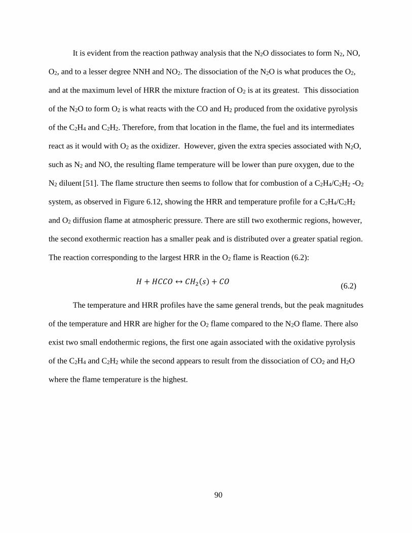
90

It is evident from the reaction pathway analysis that the N2O dissociates to form N2, NO,

O2, and to a lesser degree NNH and NO2. The dissociation of the N2O is what produces the O2,

and at the maximum level of HRR the mixture fraction of O2 is at its greatest. This dissociation

of the N2O to form O2 is what reacts with the CO and H2 produced from the oxidative pyrolysis

of the C2H4 and C2H2. Therefore, from that location in the flame, the fuel and its intermediates

react as it would with O2 as the oxidizer. However, given the extra species associated with N2O,

such as N2 and NO, the resulting flame temperature will be lower than pure oxygen, due to the

N2 diluent [51]. The flame structure then seems to follow that for combustion of a C2H4/C2H2 -O2

system, as observed in Figure 6.12, showing the HRR and temperature profile for a C2H4/C2H2

and O2 diffusion flame at atmospheric pressure. There are still two exothermic regions, however,

the second exothermic reaction has a smaller peak and is distributed over a greater spatial region.

The reaction corresponding to the largest HRR in the O2 flame is Reaction (6.2):

𝐻 + 𝐻𝐶𝐶𝑂 ↔ 𝐶𝐻2(𝑠) + 𝐶𝑂 (6.2)

The temperature and HRR profiles have the same general trends, but the peak magnitudes

of the temperature and HRR are higher for the O2 flame compared to the N2O flame. There also

exist two small endothermic regions, the first one again associated with the oxidative pyrolysis

of the C2H4 and C2H2 while the second appears to result from the dissociation of CO2 and H2O

where the flame temperature is the highest.

91

Figure 6.12: Calculated temperature and heat release rate for a C2H4/C2H2 O2 flame at



fuel surface region on the oxidizer side of the stagnation plane.

92

Figure 6.13: Calculated species profiles for a C2H4/C2H2 O2 flame at atmospheric pressure. The


counterflow burner.

Understanding the reaction and chain branching of the C2H4-O2 mechanism will shed

light as to the endothermic and exothermic events occurring in the HRR profile. Since the N2O

dissociates to form O2, which is the oxidant that reacts with the fuel, the oxidation of C2H4 was

looked at in closer depth with the O2 flame at atmospheric pressure. For ethene the major

initiation steps are

𝐶2𝐻4 + 𝑀 → 𝐶2𝐻2 + 𝐻2 + 𝑀 (6.3)

93

𝐶2𝐻4 + 𝑀 → 𝐶2𝐻3 + 𝐻 + 𝑀 (6.4)

Reaction (6.3) is the fastest however Reaction (6.4) is the chain initiator. The H

abstraction plays a major step in producing the vinyl radical (C2H3). This is shown in the reaction

pathways diagram for the pure oxygen case, where the main reaction for formation of C2H3 is

Reaction (6.4).

Figure 6.14: Reaction pathway at the endothermic heat release for the O2 flame at atmospheric

pressure located at 0.518 mm.

The majority of the vinyl is consumed by C-H bond scission to form acetylene via:

𝐶2𝐻3 + 𝑀 → 𝐶2𝐻2 + 𝐻 + 𝑀 (6.5)

94

and to a lesser extent by H-atom radical attack and the bimolecular reaction with itself.

Acetylene can be a major product of incomplete fuel rich combustion. This reaction is also

shown in the reaction pathway, which is located at the point of endothermic heat release.

Reaction (6.5) is the main contributor to this endothermic event, between, 0.5mm and 0.7mm,

seen in Figure 6.12.

The reaction between acetylene (C2H2) and O is rapid and forms the ketenyl radical

(HCCO) shown in Figure 6.15 which then proceeds to form the methylene radical (CH2) as

shown in Figure 6.16.

Figure 6.15: Reaction pathway of C2H2 near the endothermic event for O2 at atmospheric

pressure.

95

Figure 6.16: Reaction pathway at a location of 0.808mm for HCCO proceeding to the methylene

radical for oxidizer O2 at atmospheric pressure.

Since the mechanism was analyzed in closer detail, the diffusion flame structure must

also be examined. Considering the N2O flame, the stoichiometric mixture fraction is 0.1004,

located at 1.46 mm at atmospheric pressure, which is where the flame should sit. Because the

location of a diffusion flame is located at the maximum temperature, to understand the location

of the flame with respect to mixture fraction, a plot of temperature versus mixture fraction is

shown in Figure 6.17. It is clear that the flame at atmospheric pressure is not at stoichiometric

conditions. As the pressure increases the maximum temperature moves closer to the

stoichiometric mixture fraction, while also shifting slightly closer to the oxidizer side of the

96

stagnation plane of 0.7mm, 0.429 in mixture fraction space for atmospheric pressure (in

CHEMKIN a mixture fraction of zero is the oxidizer, while one corresponds to the fuel).

Figure 6.17: Temperature as a function of mixture fraction and increasing pressure for N2O.

Between 0.101 MPa and 0.448 MPa there is a shift in the maximum temperature, moving

closer to the oxidizer side of the stagnation plane. From 0.448 to 0.792 MPa the maximum

temperature occurs close to the same mixture fraction. Once the pressure reaches 1.827 MPa it is

the closest to stoichiometric conditions.

Also observed with increasing pressure is a decrease in reactant leakage, indicating a

closer approximation to reaction-sheet behavior. With increasing pressure and a decrease in

reactant leakage, more complete combustion will occur. This is understandable, as the pressure

increases the flame shifts towards the stoichiometric mixture fraction, as previously mentioned.

97

However, the flame is shown to be shifting toward the fuel side as the pressure increases. From

simple theory, a diffusion flame’s structure should be independent of pressure. Therefore, to see

if the flame’s location was moving due to the diffusion flame or the surface model coupling

implemented by the Octave wrapper, the N2O case was analyzed at a fixed momentum flux for

both the oxidizer and fuel. To obtain data for a fixed momentum case, the fuel and oxidizer

velocity was specified in CHEMKIN bypassing the wrapper. Figure 6.18 demonstrates that it is

not the diffusion flame causing the pressure dependence, but rather the physical surface model

coupling with experimental parameter inputs.

Figure 6.18: OppDiff flame calculation for fixed momentum flux for C2H4/C2H2 N2O flame. The


counterflow burner.

98

The gasification of the fuel is determined by conductive heat feedback from the gas

phase, therefore the slope of the temperature profile just above the control surface of the fuel is

what controls the burning rate. As the pressure increases, the flame becomes confined to a

thinner region with a higher flame temperature creating an increase in slope. Regression is

controlled by heat feedback, primarily conduction, at the surface, which by Fourier’s Law is

proportional to the temperature gradient, observed with rising pressures. Therefore, the increase

in regression rate due to pressure is through the slope of the temperature gradient at the surface.

The results from the modeling indicate some important observations.

1. There was an increase in linear regression rate with an increase in pressure for

C2H4/C2H2 N2O and O2 flame. The increase in regression rate with increasing

pressure is due to the slope of the temperature gradient and the increasing heat

feedback to the solid fuel surface.

2. The flame was observed to become thinner with less leakage of NO and O2

indicating faster reactions as pressure was increased.

3. The stagnation plane moved closer to the fuel side from the changing fuel

momentum flux relative to the constant momentum flux of the oxidizer with

increasing pressure. This also attributed to the larger gradient increasing heat

feedback at the fuel surface, enhancing the regression rate.

4. The flame structure of N2O exhibits the same trends as O2 following

decomposition. While the heat release from N2O decomposition and pyrolyzed

fuel oxidation occurs in two distinct regions under atmospheric conditions, but as

higher pressures are reached the exothermic heat release due to oxidation

becomes distributed over a wider spatial domain reaching larger exothermicities.

99

5. GOx was observed to have lower regression rates than N2O, due to the N2 diluent.

100

CHAPTER 7: Summary and Conclusions

Counterflow burner and static fired rocket motor experiments were conducted to

investigate HTPB and aluminized HTPB solid fuels with the oxidizers N2O and GOx at pressures

ranging from 0.101 MPa to 1.827 MPa. A detailed model using CHEMKIN and Octave was

developed to understand the flame structure and pressure dependence observed in the PCBE with

N2O. Aluminized fuel compositions were studied as well to observe any effect of the metallic

additives on solid fuel regression rates when combusted with N2O. Rocket motor experiments

were conducted to investigate propulsive performance of such fuels with N2O as the oxidizer.

PCBE experiments were conducted with HTPB and N2O, from 0.101 MPa to 1.87 MPa

and a pressure dependence on the linear regression rate was observed. The linear regression rate

increased from 0.152 to 0.21 mm/s over a pressure range of 0.101MPa to 1.1 MPa where it then

plateaued to a relatively constant value. Although the N2O decomposition process is pressure

dependent, the observed pressure dependence was found mainly to be due to heat transfer to the

pyrolyzing surface from the reaction of O2 with the fuel components, versus N2O reaction with

the fuel components. As the pressure increased, the flame shifted toward the molten fuel surface

increasing heat feedback, resulting in an increased rate of solid fuel pyrolysis. Although there

was an increase in regression rate with higher pressures, the velocity of the gasses coming off of

the solid fuel surface decreased, therefore decreasing the momentum of the fuel. The fixed

oxidizer momentum and decrease in fuel momentum caused the C2H4/C2H2 N2O flame to move

closer to the fuel surface with increasing pressure. The flame structure was also observed to

become thinner, due to faster kinetics with increasing pressure. Heat release from N2O

decomposition and pyrolyzed fuel oxidation occurs in two distinct stages under atmospheric

conditions, while at elevated pressure (1.827 MPa) the exothermic peak associated with

101

oxidation becomes distributed over a wide spatial domain containing many reactions with large

exothermicities. Following decomposition, the flame structure of N2O exhibits the same trends as

that of O2. The model results predicted experimentally measured solid fuel regression rates

within a factor of two. Furthermore, the model indicated similar trends with increasing pressure

for both the O2 and N2O, and predicted a higher regression rate for O2 as an oxidizer compared to

N2O.

Spectroscopic data obtained from aluminized counterflow burner experiments showed no

indication of AlO or Al with N2O. AlO emission was captured for experiments conducted using

GOx. This can be attributed to the lower regression rates observed with N2O not reaching

sufficient velocities to drag the particles from the molten surface to reach the flame and react.

The aluminum was not observed to ignite near the fuel surface in either counterflow burner with

N2O, overall showing a decrease in regression rate with the addition of aluminum particles to the

HTPB.

Rocket motor firings were conducted using a static-fired rocket motor to determine the

effect of the aluminum addition to HTPB fuel grains when combusted with N2O. Three solid fuel

compositions were investigated: pure HTPB and HTPB containing 10 wt% of Valimet H2 and

H12 aluminum particles. Over the baseline HTPB, the linear regression rate increased 15% for

both aluminized fuel grains. The empirical regression rate correlation was utilized for the

HTPB/H12 aluminum grains to determine a pre-exponential factor of 0.5049 compared to pure

HTPB values of 0.417 [35]. The combustion efficiency and chamber pressure for each rocket

motor experiment were similar with an average combustion efficiency of 96% achieved for the

aluminized grains. The aluminum enhanced the solid fuel regression rate in the hybrid rocket

motor, but did not show any improvement in regression rate in the counterflow burner. The

102

higher shear forces across the surface in the motor may also drag the particles along the surface

to the post combustion regime. The lack of AlO emission and observed accumulation of

aluminum particles in the surface melt in the counterflow burners suggests the velocity of the

gaseous pyrolysis products evolving from the fuel surface was insufficient to drag the particles

from the viscous surface melt. Slower regression rates would also indicate a thicker melt layer,

where more particles could accumulate. Future experiments should be considered employing

higher oxidizer velocities to determine whether aluminum particle entrainment can be achieved,

and enhanced regression rate result using the counterflow configuration.

103

7.1 Future Work Recommendations

1) Extend the experiments in the PCBE with N2O to higher pressures and higher

oxidizer flow rates. This will shed light onto whether or not the linear regression rate

will continue to plateau. By obtaining higher oxidizer velocities this will increase the

linear regression rate, in turn increasing the velocity of the gaseous pyrolysis products

evolving from the fuel surface, to determine what velocity is needed to entrain the

aluminum in the flame.

2) To obtain regression rates in the model the surface temperature was held constant.

Given the Arrhenius kinetics provided, the regression rate only varied 3% with a 5%

change in surface temperature. However, the products from the pyrolysis reaction are

known to shift significantly with temperature. Therefore, it would be valuable to

modify the condensed phase model to include the change in surface products, with

varying surface temperature. The code can be altered to calculate the temperature

from the Arrhenius expression for a given regression rate. Given the surface

temperature the species evolving from the HTPB surface can be inputted into the

model. A micro-thermocouple embedded into the pellet to measure the temperature

profile as the surface regresses will allow for a more accurate understanding of the

experimental condition to be observed.

3) Compare the C2H4/C2H2 N2O flame to a C2H4/C2H2 N2/O2 flame to understand the

effect of oxidizer exothermic decomposition, and N2 dilution on the regression rates

and flame structure.

4) Modify the condensed phase and gas-phase models to consider metal particles in the

solid fuel, this will help understand the effect condensed phase particles have on the

104

regression rate, through radiation and the added heat of combustion. This can be

accomplished using Data Parallel Line Relaxation CFD code (DLPR) to couple the

condensed phase particles to the gas-phase model.

105

References

[1] G. P. Sutton, Rocket Propulsion Elements, New York: John Wiley and Sons, 2001.

[2] M. Chiaverini, "Regression Rate and Pyrolysis Behavior of HTPB-Based Solid Fuels in a

Hybrid Rocket Motor," The Pennsylvania State University, 1997.

[3] D. Pastrone, "Approaches to Low Fuel Regression Rate in Hybrid Rocket Engines,"

International Journal of Aerospace Engineering, vol. 2012, p. 13, 2012.

[4] G. Risha, "Enhancement of Hybrid Rocket Combustion Performance Using Nano-Sized

Energetic Particles," Ph. D. Dissertation, Pennsylvania State University, 2003.

[5] H. S. Committee, "Hybrid Rocket Propulsion: Report of an AIAA Workshop,"

Washington, D.C., 1995.

[6] R. H. Johansson, "Investigation of Solid Oxidizer and Gaseous Fuel Combustion

Performance Using an Elevated Pressure Counterflow Experiment and Reverse Hybrid

Rocket Engine," Pennsylvania State University, 2012.

[7] E. Price and R. K. Sigman, "Combustion of Aluminized Solid Propellants," AIAA, vol. 185,

no. Solid Propellant Chemistry, Combustion, and Motor Interior Ballistics, pp. 663-687,

2000.

[8] G. A. Risha, B. J. Evans, E. Boyer and K. K. Kuo, "Metals, Energetic Additives, and

Special Binders Used in Solid Fuels for Hybrid Rockets," AIAA, vol. Chapter 10, pp. 430-

167.

[9] E. Price, "Combustion of Metallized Propellants," Progress in Astronautics and

Aeronautics, vol. 90, pp. 479-513, 1983.

[10] M. Beckstead, "Lectures on Metal Combustion," China Lake, CA, 1999.

[11] E. L. Dreizin, M. Schoenitz and A. Mikhaylo, "Ignition of Aluminum Powders Under

Different Experimental Conditions," Propellants, Explosives, Pyrotechnics, vol. 1, no. 30,

2005.

[12] J. Katz, "Metastable nanosized aluminum powder as a reactant in energetic formulations,"

JANNAF Propulsion Meeting, Cleveland, OH, 1998.

[13] G. P. Sutton and O. Biblarz, "Rocket Propulsion Elements," in Rocket Propulsion

Elements, Wiley, 2000, p. 581.

[14] "Penn Hybrid Rocket," University of Pennsylvania, [Online]. Available:

https://sites.google.com/site/pennhybridrocket/how-do-hybrid-rocket-motors-work .

[Accessed 12 December 2015].

[15] "Liquid Oxygen," Air Products, November 2015. [Online]. Available:

http://www.airproducts.com/~/media/files/pdf/company/safetygram-6.pdf. [Accessed 13

January 2016].

[16] "Space Safety Magazine," 1 November 2014. [Online]. Available:

http://www.spacesafetymagazine.com/aerospace-engineering/rocketry/hybrid-rocket-

overview-part-2/. [Accessed 25 December 2015].

[17] "Nitrous Oxide Safety," Space Propulsion Group, 2012. [Online]. Available:

http://www.spg-corp.com/nitrous-oxide-safety.html. [Accessed 25 December 2015].

[18] G. Marxman and M. Gilbert, "Turbulent Boundary Layer Combustion in the Hybrid

106

Rocket," Symposium (International) on Combustion, vol. 9, pp. 371-383, 1963.

[19] S. Shark, "Solid-Fuel Regression Rates and Flame Characterstics in an Opposed Flow

Burner," Journal of Propulsion and Power, pp. 1-10, 2014.

[20] M. Khattab, "Innovative Solid Fuels for Hybrid Rocket Propulsion," 2010.

[21] C. Law, "Counterflow Flame," in Combustion Physics, New York, Cambridge, 2006, pp.

224-229.

[22] "Lecture8," Institut fur Technische Verbrennung, [Online]. Available:

https://www.princeton.edu/cefrc/Files/2010%20Lecture%20Notes/Norbert%20Peters/Lectu

re8.pdf. [Accessed 12 December 2015].

[23] C. Law, Combustion Physics, New York: Cambridge University Press, 2006.

[24] G. Young, "Combustion of Alane-Based Solid Fuels," International Journal of Energetic

Materials and Chemical Propulsion, vol. 9, pp. 249-266, 2010.

[25] I. K. Puri and K. Seshadri, "Extinction of Diffusion Flames Burning Diluted Methane and

Diluted Propane in Diluted Air," Combustion and Flame, vol. 65, pp. 137-150, 1986.

[26] Courtesy of Dr.Young, Indian Head , 2015.

[27] H. K. Chelliah, C. K. Law, T. Ueda, M. D. Smooke and F. A. Williams, "An Experimental

and Theoretical Investigation of the Dilution, Pressure and Flow Field Effects on the

Extinction Condition of Methane-Air-Nitrogen Difusion Flames," 23rd Symposium

(International) on Combustion. vol. 23, no. 1, pp. 503-511, 1990.

[28] D. Armold, "Formulation and Characterization of Paraffin Based Solid Fuels Containing

Swirl Inducing Grain Geometryand/or Energetic Additives," Pennsylvania State University,

2014.

[29] D. Armold, E. Boyer, B. McKnight, K. Kuo, J. DeSain, J. Fuller , B. Brady and T. Curtiss,

"Performance Chracterization of Hybrid Rocket Fuel Grains with Complex Port

Geometries Fabricated Using Rapid Prototyping Technology," International Journal of

Energetic Materials and Chemical Propulsion, vol. 13, pp. 287-387, 2014.

[30] McBride, G. Sanford and J. Bonnie, "Computer Program for Calculation of Complex

Chemical Equilibrium Compositions and Applications I. Analysis," Cleveland, OH, 1994.

[31] W. Kalback, "The Thermal Decomposition of Nitrous Oxide on Gold at Elevated

Pressures," University of Oklahoma, Oklahoma, 1973.

[32] R. J. Kee, F. M. Rupley, J. A. Miller, M. E. Coltrin, J. F. Grcar, H. K. Meeks, A. E. Moffat,

G. Lutz, M. D. Dixon-Lewis, J. Smooke, G. H. Warnatz, G. H. Evans, R. S. Larson, R. E.

Mitchell, L. R. Petzold, W. C. Reynolds, M. Caracotsios, W. E. Stewart, P. Glarborg, C.

Wang, O. Adigun, W. G. Houf, Chou, S. F. Miller, P. Ho and D. F. Young, "Chapter 3: Gas

Phase Chemical Rate Expressions," in Reaction Design Theory Manual, San Diego,

CHEMKIN Release 4.0, Reaction Design, Inc, 2004.

[33] "Theories of Unimolecular Reaction Rates," [Online]. Available:

http://vallance.chem.ox.ac.uk/pdfs/UnimolecularReactionNotes.pdf. [Accessed 9 January

2016].

[34] C. Carmicino, F. Scaramuzzino and S. A. Russo, "Trade-off between paraffin-based and

aluminum loaded HTPB fuels to improve performance of hybrid rocket fed with N2O,"

Aerospace Science and Technology, vol. 37, pp. 81-92, 2014.

[35] E. Doran, J. Dyer, K. Lohner, Z. Dunn, B. Cantwell and G. Zilliac, "Nitrous Oxide Hybrid

107

Rocket Motor Fuel Regression Rate Characterization," 43rd AIAA/ASME/SAE/ASEE Joint

Propulsion Conference & Exhibit, 2007.

[36] M. Chiaverini, G. C. Harting, Yeu-Cherng Liu, K. K. Kuo and A. Peretz, "Pyrolysis

Behavior of Hybrid-Rocket Solid Fuels Under Rapid Heating Conditions," Journal of

Propulsion and Power, vol. 15, no. 6, 1999.

[37] Y. K, "Thermal Decomposition Study of HPTB Solid Fuel in the Presence of Activated

Charcoal and Paraffin," Journal of Thermal Analysis and Calorimetry, vol. 119, no. 1, pp.

557-565, 2015.

[38] J. Boyer, "Combustion Characteristics and Flame Structure of Nitromethane Liquid

Monopropellant," Pennsylvania State University, 2005.

[39] G. A. Marxman, C. E. Wooldridge and R. J. Muzzy, "Fundementals of Hybrid Boundary

Layer Combustion," Heterogeneous Combustion, Progress in Astronautics and

Aeronautics, vol. 15, pp. 485-521, 1964.

[40] L. Galfetti, "Innovative Solid Fuels," [Online]. Available:

https://www.politesi.polimi.it/bitstream/10589/28081/1/KHATTAB.pdf . [Accessed 24

December 2015].

[41] M. Chiaverini, "Regression Rate and Pyrolysis Behavior of HTPB-Based Solid Fuels in a

Hybrid Rocket Motor," Pennsylvania State University, 1997.

[42] S. D. Chambreau, J. Lemieux, L. Wang and J. Zhang, "Mechanistic Studies of the Pyrolysis

of 1,3-Butadiene-1,1,4,4,-d4 1,2-Butdadiene, and 2-Butyne by Supersonic

Jet/Photoionization Mass Spectrometry," J. Phys. Chem., pp. 2190-2196, 2005.

[43] A. Lutz, R. J. Kee, J. F. Grcar and F. M. Rupley, "OPPDIFF: A Fortran program for

computing opposed-flow diffusion flames," May 1997. [Online]. Available:

http://www.osti.gov/scitech/servlets/purl/568983/. [Accessed 24 December 2015].

[44] P. Glarborg, "Chemistry and Mixing Effects in Reburning," 1999. [Online]. Available:

http://www.dgc.eu/sites/default/files/filarkiv/documents/R0011_chemistry_mixing_effects.

pdf. [Accessed 12 December 2015].

[45] "Gas Encyclopedia," [Online]. Available:

http://encyclopedia.airliquide.com/encyclopedia.asp?GasID=29&CountryID=18&Languag

eID=11. [Accessed 1 Febrauary 2016].

[46] "Gas Encyclopedia," [Online]. Available:

http://encyclopedia.airliquide.com/encyclopedia.asp?GasID=29&CountryID=18&Languag

eID=11. [Accessed 19 February 2016].

[47] "DIPPR," AIChE, 2001. [Online]. Available:

http://dippr.byu.edu/public/chemsearch.asp?Mode=Printout2&ChemID=201. [Accessed 18

October 2015].

[48] T. N. Lehman, R. Grana, K. Seshadri and F. Williams, "The structure and extinction of

nonpremixed methane/nitrous oxide and ethane/nitrous oxide flames," Proceedings of the

Combustion Institute, pp. 2147-2153, 2013.

[49] I. Glassman, R. Yetter and N. Glumac, Combustion, Elsevier Science , 2014.

[50] "Deomposition of Carbon Dioxide," 2012. [Online]. Available:

http://carbon.atomistry.com/decomposition_carbon_dioxide.html. [Accessed 2 December

2015].

108

[51] C. Lee, Environmental Engineering Dictionary, Lanham: Scarecrow Press, 2005.

109

Appendix A: Sample of NASA CEA Code Input and Output Files

Input File: problem

o/f=1.11

rocket equilibrium

tcest,k=3000

p,psia=400

sup,ae/at=20

react

oxid=O2 wt=1 t,k=298

fuel=HTPB wt=0.8200 t,k=298 h,kj/mol=-12.43 C 7.337 H 10.981 O 0.058

fuel=AL(cr) wt=0.1764 t,k=298

fuel=AL2O3(a) wt=0.0036 t,k=298

output

siunits

plot p t isp ivac m mw

end

Output File: Pin = 400.0 PSIA

CASE =

REACTANT WT FRACTION ENERGY TEMP

(SEE NOTE) KJ/KG-MOL K

OXIDANT O2 1.0000000 -4.407 298.000

FUEL HTPB 0.8200000 -12430.000 298.000

FUEL AL(cr) 0.1764000 -3.630 298.000

FUEL AL2O3(a) 0.0036000 -1675711.854 298.000

O/F= 1.11000 %FUEL= 47.393365 R,EQ.RATIO= 2.502418 PHI,EQ.RATIO= 2.514999

CHAMBER THROAT EXIT

Pinf/P 1.0000 1.7671 229.82

P, BAR 27.579 15.607 0.12000

T, K 2977.80 2745.16 1090.71

RHO, KG/CU M 2.2046 0 1.3619 0 2.6794-2

H, KJ/KG -76.373 -758.65 -4483.28

U, KJ/KG -1327.35 -1904.57 -4931.15

G, KJ/KG -35115.7 -33060.6 -17317.5

S, KJ/(KG)(K) 11.7669 11.7669 11.7669

M, (1/n) 19.792 19.918 20.249

MW, MOL WT 19.290 19.362 19.503

(dLV/dLP)t -1.00642 -1.00373 -1.00757

(dLV/dLT)p 1.1426 1.0870 1.1235

Cp, KJ/(KG)(K) 3.5401 3.0086 2.6611

GAMMAs 1.1744 1.1908 1.2303

SON VEL,M/SEC 1212.1 1168.1 742.3

MACH NUMBER 0.000 1.000 3.999

PERFORMANCE PARAMETERS

Ae/At 1.0000 20.000

CSTAR, M/SEC 1733.5 1733.5

CF 0.6739 1.7126

Ivac, M/SEC 2149.1 3119.7

Isp, M/SEC 1168.1 2968.8

110

MOLE FRACTIONS

*AL 0.00109 0.00058 0.00000

ALH 0.00037 0.00020 0.00000

*ALO 0.00006 0.00002 0.00000

ALOH 0.00513 0.00244 0.00000

AL(OH)2 0.00001 0.00000 0.00000

AL2O 0.00152 0.00076 0.00000

AL2O2 0.00002 0.00000 0.00000

CH4 0.00000 0.00000 0.00083

*CO 0.54818 0.55081 0.54455

*CO2 0.00117 0.00058 0.00382

*H 0.01741 0.01067 0.00000

HCO 0.00002 0.00001 0.00000

*H2 0.39342 0.40303 0.41117

H2O 0.00616 0.00292 0.00284

*OH 0.00010 0.00002 0.00000

AL2O3(a) 0.00000 0.00000 0.03054

AL2O3(L) 0.02534 0.02793 0.00000

C(gr) 0.00000 0.00000 0.00626

* THERMODYNAMIC PROPERTIES FITTED TO 20000.K

PRODUCTS WHICH WERE CONSIDERED BUT WHOSE MOLE FRACTIONS

WERE LESS THAN 5.000000E-06 FOR ALL ASSIGNED CONDITIONS

ALC ALC2 ALH2 ALH3 ALO2

AL(OH)3 AL2 AL2C2 AL2O3 *C

*CH CH2 CH3 CH2OH CH3O

CH3OH CH3OOH COOH *C2 C2H

C2H2,acetylene C2H2,vinylidene CH2CO,ketene O(CH)2O HO(CO)2OH

C2H3,vinyl CH3CO,acetyl C2H4 C2H4O,ethylen-o CH3CHO,ethanal

CH3COOH OHCH2COOH C2H5 C2H6 C2H5OH

CH3OCH3 CH3O2CH3 C2O *C3 C3H3,1-propynl

C3H3,2-propynl C3H4,allene C3H4,propyne C3H4,cyclo- C3H5,allyl

C3H6,propylene C3H6,cyclo- C3H6O,propylox C3H6O,acetone C3H6O,propanal

C3H7,n-propyl C3H7,i-propyl C3H8 C3H8O,1propanol C3H8O,2propanol

C3O2 *C4 C4H2,butadiyne C4H4,1,3-cyclo- C4H6,butadiene

C4H6,1butyne C4H6,2butyne C4H6,cyclo- C4H8,1-butene C4H8,cis2-buten

C4H8,tr2-butene C4H8,isobutene C4H8,cyclo- (CH3COOH)2 C4H9,n-butyl

C4H9,i-butyl C4H9,s-butyl C4H9,t-butyl C4H10,n-butane C4H10,isobutane

*C5 C5H6,1,3cyclo- C5H8,cyclo- C5H10,1-pentene C5H10,cyclo-

C5H11,pentyl C5H11,t-pentyl C5H12,n-pentane C5H12,i-pentane CH3C(CH3)2CH3

C6H2 C6H5,phenyl C6H5O,phenoxy C6H6 C6H5OH,phenol

C6H10,cyclo- C6H12,1-hexene C6H12,cyclo- C6H13,n-hexyl C6H14,n-hexane

C7H7,benzyl C7H8 C7H8O,cresol-mx C7H14,1-heptene C7H15,n-heptyl

C7H16,n-heptane C7H16,2-methylh C8H8,styrene C8H10,ethylbenz C8H16,1-octene

C8H17,n-octyl C8H18,n-octane C8H18,isooctane C9H19,n-nonyl C10H8,naphthale

C10H21,n-decyl C12H9,o-bipheny C12H10,biphenyl HALO HALO2

HCCO HO2 HCHO,formaldehy HCOOH H2O2

(HCOOH)2 *O *O2 O3 AL(cr)

AL(L) ALH3(a) AL(OH)3(a) AL4C3(cr) H2O(cr)

H2O(L)

NOTE. WEIGHT FRACTION OF FUEL IN TOTAL FUELS AND OF OXIDANT IN TOTAL OXIDANTS

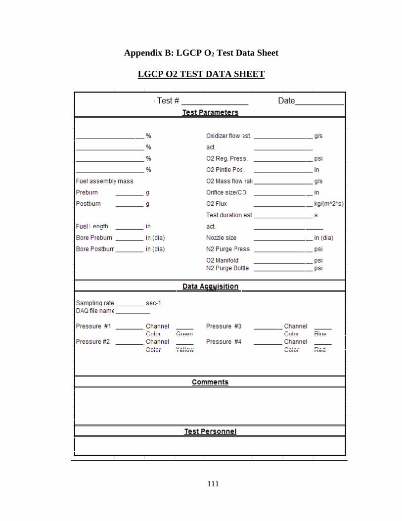
111

Appendix B: LGCP O2 Test Data Sheet

LGCP O2 TEST DATA SHEET

11.5

11.5

112

O2 Manifold Open

O2 Manifold Shut

O2 Run Open

O2 Run Shut

N2 Purge Open

N2 Purge Shut

Igniter Energize

Igniter Deenergize

113

Appendix C: LGCP Checklist for Motor Firing

CHECKLIST FOR O2 LGCP MOTOR FIRING

Oxygen LGCP Hybrid Rocket Motor Test Setup Procedure:

Turn on the overhead fan and place a box fan near the run tank.

Verify sufficient reserves of nitrogen and oxygen in bottles.

Mount the outdoor test camera, install A/V lines.

Setup a video camera and TV with a DVD recorder to record the motor firing.

Title the DVD video display and set DVD to a new recording.

Ensure proper size burst disk is installed.

Verify the shop air is connected to all remotely operated valves and greater than 90 psig in

room 127 (___________ psig).

Plug in and turn on the power supply to patch panel. This is located beneath the mounting

platform for the motor.

Ensure all signal cables are connected and turn on the data acquisition system (Nicolet

Vision).

Verify sampling rate is 1 ks/s.

Ensure all pressure transducers show appropriate baseline values on the data acquisition

system (around 0psig +/-5).

Ensure oxygen pintle on venturi is set to 2” (or full open).

Ensure nitrogen purge line hand ball valve is aligned to LGCP.

With the control board off, open the control program, “Hybrid Slab Motor Control V10.vi”.

Verify that program is in “Automatic” mode

114

Start the program (upper left corner).

Turn on the control board and ensure all valve indication and fuse lights are lit

Ensure Oxygen run valve (light off) and nitrogen purge (light on) are shut.

Testing Procedure:

Ensure all non-testing personnel are clear from the test cell and fenced-in area.

Remove block from load cell.

Open nitrogen purge bottle and set regulator to amount specified on test data sheet (~300psi

greater than O2 regulator).

Open reference pressure nitrogen bottle attached to oxygen regulator.

Verify oxygen line hand valve and cluster hand valves with bottles are open (and hand valves

leading to other systems are shut).

Power on reference pressure digital readout.

Slowly open oxygen bottle valves.

Set oxygen regulator to value written on test data sheet (slightly lower)

Insert the fuel grain, post-combustion chamber, and nozzle plug into the chamber.

Insert the graphite filler pieces, electric match, and injector plug into the chamber.

Make an announcement for starting the test firing: “We will be conducting a motor firing in

room 127. Please stand clear of the test cell and the fenced-in area.”

Connect igniter lines to electric match leads.

Slid motor back so it is resting on load cell.

Check ALL timing parameters.

Re-check all regulators.

Press “Record” on the DVD and start timer on title screen.

115

Press “Record” on the data acquisition system.

Press “Record” on Hybrid Slab Motor Control V.10.vi.

Ensure all lights necessary for LGCP test are illuminated.

Use the control program to initiate the test.

**************************TEST INITIATED******************************

If misfire occurs, stop using this portion of checklist and move onto the Misfire Procedure

section.

*************************TEST CONCLUDED*****************************

Press “Stop” on DVD recorder and data acquisition systems.

Check that all valves have shut.

Replace block for load cell.

Disassemble motor, remove fuel grain, and secure injector plug to motor chamber.

If additional tests are to be completed, move to the New Test section.

Announce “We will now be venting gases in room 127, all personnel stay clear”.

Secure the injector plug to the LGCP chamber.

Close oxygen bottles at the cluster.

With the igniter, fuel grain, and graphite pieces removed, using the manual mode of operation

of the control program, open the oxygen run valve, wait a few seconds then allow manifold valve

to vent.

Close the oxygen run valve.

Close nitrogen bottle purge bottle.

Using the manual mode of operation of the control program, open the nitrogen purge valve to

allow nitrogen lines to vent.

116

Announce “Test completed in room 127”

Close and vent the nitrogen regulator being used for O2 pressure regulation.

Check to ensure no back pressure in O2 manifold.

Turn off the patch panel power supply.

Turn off O2 reference pressure digital readout.

Quit the Hybrid Slab Motor Control V10.vi control program.

Turn off the control board.

Close shop air ball valve in the machine shop.

Replace block for load cell.

Misfire Procedure:

Immediately turn off hybrid control board by turning key; this will start nitrogen flow and

interrupt oxygen flow.

Announce “Misfire has occurred in room 127, stay clear of the test cell and fenced in area

until directed otherwise”.

Continue nitrogen flow for at least 15 seconds.

Continue recording event on outdoor camera.

On the control program; restart and turn on manual mode and ensure all relays are in the shut

position.

Turn on control panel. Verify all flows have stopped and no smoldering is observed. If

smoldering is observed, continue to purge the system using the manual control.

Isolate oxygen by closing oxygen bottles at the cluster.

Press “Stop” on the data acquisition system.

117

Record time of misfire.

Verify combustion has subsided via outdoor camera.

After 10 minutes personnel may enter test chamber.

Announce “Test completed in room 127”.

Gather evidence and determine cause of problem.

New Test:

Close oxygen hand valve.

Close N2 Purge Bottle.

Reload motor

If next test is at a lower pressure vent O2 and N2 lines manually.

Reopen O2 hand valve.

Follow testing procedure for next test.

118

Appendix D: O2 LGCP Motor Setup Walkthrough

Oxygen Tubing (in order):

Oxygen Manifold (RM 128)

119

Oxygen Pressure Regulator (RM 128)

Oxygen Hand Valve (RM 128)

To

RM 127

120

Nitrogen Reference for Oxygen Pressure Regulator (RM 128)

Oxygen Manifold Valve (RM 127)

121

Oxygen Line (RM 127)

122


Oxygen Venturi Pintle (RM 127)

123

Oxygen Run Valve (RM 127)


124


125


Oxygen into Orifice Setup (RM 127)

126

Oxygen into Motor (RM 127)

Nitrogen Tubing (in order):

127

Nitrogen Purge Bottle and Regulator (RM 128)

Nitrogen Line (RM 128)

128

Nitrogen Purge Valve (RM 128)

To

RM 127

129



130



131

Nitrogen Ball Valve (RM 127)

132



133


Nitrogen into Orifice Setup (RM 127)

134

Nitrogen into Motor (RM 127)

Electrical:

135

Panel for BNC Cables (RM 127)

BNC Wires (RM 127)

136

BNC and Igniter Wires (RM 127)

137

BNC and Igniter Wires (RM 127)

BNC and Igniter Wire Feedthrough to Control Room (RM 127)

138

BNC and Igniter Wire Feedthrough to Control Room (Control Room)

Relays (Control Room)

139

Relay Wires (Control Room)

140

Relay Wire Feedthrough Box (Control Room)

Relay Wire Feedthrough Box (RM 127)

141

Relay Wires (RM 127)

Relay Wires (RM 127)

142

Relay Wire Box to Valves (RM 127)

143

Relay Wires to Valve (RM 127)

Relay Wires to Valve (RM 128)

144

Appendix E: LGCP Firings of Aluminized Fuel Grains

The main focus of conducting experiments with the aluminized fuel grains with GOx was

to obtain regression rates and combustion efficiencies for 18 and 40 wt% aluminum HTPB fuel

grains. Two different aluminums were used for manufacturing the fuel grains: H30 from Valimet

and X-85 from Toyal, both being 61.27µm in diameter. This gave the ability to see if there were

any changes in regression rates and combustion efficiency between the two manufacturers. For

the motor firings, an initial GOx value of 780 kg/m2s was required (one of the requirements for

testing from NASA Jacobs) as well as a chamber pressure between 2.75-4.14 MPa (400-600

psia). The fuel length, oxidizer flow rate were all picked based upon the optimum O/F that

corresponded to the highest Isp. Figure E.1 below displays HTPB with aluminum loading up to

40% for a range of O/F values.

145

Figure E.1: HTPB aluminized fuel grains Isp as a function of O/F.

Shown in Figure E.1 the optimum O/F for pure HTPB is 2, while it is 1.6 and 1.2 for 18

and 40 wt%, respectively. Given an initial GOx value and the optimum O/F, the fuel grain length

can be calculated. The planning Excel sheet was used to calculate all the requirements for the

rocket motor firings. After completion of each firing, the fuel grain was removed and inspected

for even regression. After firing the first three fuel grains it was noticed that they were burning

unevenly, with pockets of fuel gouging out of the center. This can be observed in Figure E.2

along with one actual rocket motor test that burned evenly.

146

Figure E.2: Uneven and even post-burn of 18% aluminized fuel grains.

Due to this uneven regression, the fuel grains that were not tested were taken and X-

rayed. Upon completion of X-raying the fuel grains it was found that the fuel grains had

detachment issues as well as flaws. Below in Figure E.3 is an example of an X-ray image where

the fuel grain appeared to be detached from the phenolic casing. To see if this was actually the

case, that specific fuel grain was sectioned in half. Figure E.4 displays the sectioned fuel grain,

where it is visible that the fuel grain was detaching away from the phenolic casing.

Figure E.3: X-ray image of detaching fuel grain away from phenolic tubing.

147

Figure E.4: Sectioned fuel grain that was X-rayed and found to be detaching away from the

phenolic casing.

Not only were some of the fuel grains detaching, but there were radial flaws along the

center port of the grain in Figure E.5. Again this fuel grain was sectioned, displaying the radial

flaws that were discovered in the X-ray image in Figure E.6.

Figure E.5: X-ray image of fuel grain with radial flaws.

148

Figure E.6: X-rayed fuel grain in Figure E.5 taken and sectioned to display radial flaws.

To ascertain if the uneven burning rate was due to the flaws and detachment issues found

from the X-ray imaging, two fuel grains were chosen to conduct a firing; one with no observed

flaws in the X-ray images and one with flaws. It was hypothesized that the issues that were

showing up with the uneven burning were due to the flaws from casting.

As hypothesized, the grain without any flaws seen in the X-ray images burned evenly

while the one with flaws did not. Out of the eighteen grains sent to the HPCL, only seven were

tested due to the issues found with the casting. The data were reduced and analyzed as described

in section 4.2. With all of the uneven burning, however, it was hard to get accurate

149

measurements for the linear regression rate. This caused a significant amount of scatter in the

data. A summary of the test results is provided in Table E.1. The resulting linear and mass

regression rate data for the aluminized grains are plotted in Figure E.7 and Figure E.8.

Table E.1: Aluminized fuel grain test results.

Figure E.7: Averaged linear regression rate for aluminized hybrid fuel grains with respect to the

average oxidizer mass flux compared to Risha et al.

Fuel Length (in)Avg. Chamber

Pressure (psig)Avg. O/F

Initial GOx

(kg/m^2-s)

Avg. GOx

(kg/m^2-s)

Avg. Regression

Rate (mm/s)

Avg. Mass

Regression (kg/s)

c* Combustion

Efficiency

18% Al HTPB [627B-1] 5 340 2.745 744 68.2 1.43 0.008582 1.008

18% Al HTPB [627A-1] 5 289 2.42 737 96 1.36 0.009631 0.892

18% Al HTPB [627A-2] 6 265 2.54 743 121 1.195 0.009263 0.8334

18% AL HTPB [627B-2] 6 256 2.43 744 115 1.23 0.009683 0.7389

18% Al HTPB [627B-1] 12 584 1.11 745 123 1.119 0.02127 0.9578

18% Al HTPB [627A-1] 12 632 1.1 744.9 112 1.244 0.024122 0.9954

18% Al HTPB [627A-2] 12 539 1.17 739.01 112 1.14 0.0199 0.996

18% Al HTPB [627B-2] 12 514 1.52 750 110 1.08 0.02015 0.9617

18% Al HTPB [627B-3] 12 629 1.03 738 133 1.077 0.02263 1.01

40% AL HTPB [627C-2] 10.5 480 1.14 740 110 1.229 0.0205 0.88

40% Al HTPB [627D-1] 7 523 1.67 742 106 1.283 0.014 1.1

NASA_SFT Test Results Summary

150

Figure E.8: Averaged mass regression rate for aluminized hybrid fuel grains with respect to the

average oxidizer mass flux in comparison to Risha et al.

Although there was scatter in both the linear and mass regression rates, it comes close to

the data collected from Dr. Risha who got the aluminum from a different manufacturer in a

slightly smaller size, NTECH-50 nm at 20 wt% [4]. However, the data are inconclusive. The

linear regression rate decreases as the oxidizer mass flux is increased. The linear regression rate

should be increasing with increasing oxidizer flux, as seen with Risha. The mass regression rate

seems to be a more viable option given the fact that the mass was measured for pre and post-test,

however, there is too much scatter in the data to make any conclusions and comparisons.

Therefore, since the fuel grains mass was measured pre- and post-testing the mass

average burning rate was converted to a linear burn rate. This still proved to be unreliable due to

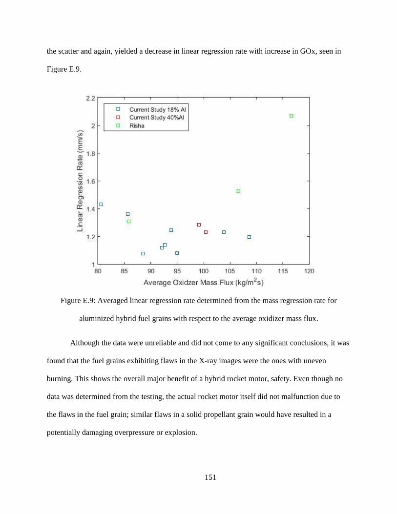
151

the scatter and again, yielded a decrease in linear regression rate with increase in GOx, seen in

Figure E.9.

Figure E.9: Averaged linear regression rate determined from the mass regression rate for

aluminized hybrid fuel grains with respect to the average oxidizer mass flux.

Although the data were unreliable and did not come to any significant conclusions, it was

found that the fuel grains exhibiting flaws in the X-ray images were the ones with uneven

burning. This shows the overall major benefit of a hybrid rocket motor, safety. Even though no

data was determined from the testing, the actual rocket motor itself did not malfunction due to

the flaws in the fuel grain; similar flaws in a solid propellant grain would have resulted in a

potentially damaging overpressure or explosion.

152

Appendix F: Octave Wrapper Code

%Paige Nardozzo

%Start Datae: 11/30/2105

%End Date: 2/28/2016

%PROGRAM: CHEMKIN_opposed_flow

%PURPOSE: Entry point for the console application

clear

clc

more off %since Octave doesn't display stuff within the while loop until it is finished

%use more off to make sure it goes straight to the screen and displays everything

%while it is running.

%Execution parameters and other user settings

maxloops = 5;

%Ti = 298 ;%initial temperature (k)

%Set filenames to use

%therm_data_file = 'therm.dat' ;%Therm file name

%therm_output_file = 'therm_output_file' ;%Therm output filename

%trans_data_file = 'trans.dat' ;%Trans data file

%trans_input_file = 'trans_input_file' ;% transport data file

%trans_output_file = 'trans_output_file' ;%trans output file

%chem_input_file = 'chem_input_file' ;%chem input file

%chem_output_file = 'chem_output_file' ;%Chem output file

%oppdiff_input_file = 'OppDiff_HTPB_N2O.inp' ;%premix input file

%***Start body of program****

%*Initialize shell environment

[N, R, Q, F] = Set_CHEMKIN_env () % Function for setting up the environment variables for CHEMKIN

%*Initialize variables

delta_rb = 1e0; %Initialize to some huge value so convergence loop runs...

rb_tol = 1e-6;

loopcount = 0 ;

error_message = ''

%* Preprocess chemistry meachansim, therm, and transport data files

% Preprocess chem.inp mechanism file and therm.dat data file (this is explained

% in "Getting Started 4.3")

% status = system('%REACTION_DIR%\chemkin15141_win64\bin\chem -i chem.inp -o chem.out

% & -d %REACTION_DIR%\chemkin15141_win64\data\therm.dat')

% [status,cmdout] = system('%REACTION_DIR%\chemkin15141_win64\bin\chem -i Glarborg_hc_no_reburn.inp

-o Glarborg_hc_no_reburn.out -d %REACTION_DIR%\chemkin15141_win64\data\therm.dat')

[status,cmdout] = system('%REACTION_DIR%\chemkin15151_win64\bin\chem -i Glarborg_hc_no_reburn.inp -o

Glarborg_hc_no_reburn.out -d %REACTION_DIR%\chemkin15151_win64\data\therm.dat')

disp('Preprocessed chemistry and therm data files....')

153

%Preprocess tran.dat file

%[status,cmdout] = system('%REACTION_DIR%\chemkin15141_win64\bin\tran -o tran.out -d tran2.dat')

[status,cmdout] = system('%REACTION_DIR%\chemkin15151_win64\bin\tran -o tran.out -d tran2.dat')

disp('Preprocesssed transport data file')

%**Main loop - checks rb match for convergence between assumed value and calculated

%value from gas phase heat transfer

%Put in a do loop/while loop to make sure that it keeps on iterating if delta_rb>rb_tol

while abs(delta_rb>rb_tol)

%Check to see if maximum number of loops reached loopcount is acting

%strange and i set it to start at 0 but autamtically jumps to 1 but it used

%the case to run the opposed flow burner of loopcount=0 is this a problem?

if (loopcount==maxloops)

X = ['Loopcount=', num2str(loopcount)];

disp(X) %other parameters of interest for problem-solving

eror_message='Maximum loopcount reached with no convergence.'

break

endif

% ** Run opposed flow burner diffusion CHEMKIN program

if (loopcount==0)

%run PREMIX to find new solution

[status,cmdout2] = system('%CHEMKIN_BIN%\CKReactorOpposedFlow -i OppDiff_HTPB_N2O22.inp -o

OppDiff_HTPB_N2O22.out')

disp('CKReactorOpposedFlow executed')

elseif %if loopcount>0 run PREMIX with restart file and new input file

[status,cmdout3] = system('%CHEMKIN_BIN%\CKReactorOpposedFlow -i OppDiff_HTPB_N2O22.inp -o

OppDiff_HTPB_N2O22.out')

disp('CKReactorOpposedFlow with restart executed')

endif

%Check for succesful execution

%Check for existence of XMLDate.zip file

C = exist('XMLData.zip', 'file')

if (C == 0)

disp('No XMLData.zip file exists...please check input files and output')

disp('logs for possible errors, then restart')

error_message = 'Missing XMLData.zip'

break

endif

%Check for existence of executuable output logfile and look for signs of success

D = exist('OppDiff_HTPB_N2O22.out','file')

if (D == 0)

disp('No oppdiff.out file exists please check input files and output')

disp('logs for possible errors, then restart')

error_message = 'Missing output logfile'

break

endif

%Check for indication of successful convergence in CHEMKIn app output file:

154

%'TWOPNT: SUCCESS. PROVLEM SOLVED.' seen at end of output for good run,

%so search for substring with this line.

%*be careful with this--look at some output files to make sure it doesn't

%converge, refine the grid, then *not* converge for final case. May need to

%go to end of output file, rewind a few lines, and scan them to make sure

%only final status of TWOPNT is caputred

%Pattern = 'TWOPNT: SUCCESS'

%A = fileread('OppDiff_HTPB_N2O.out')

%B = strfind(A,Pattern)

%empty = [] %what B will spit out an empty matrix if the pattern is not

%found in the file

%if isequal(size(empty), size(B))

%disp('No TWOPNT success found...may be a convergence problem')

%error_message = 'No TWOPNT: SUCCESS found'

%break

%else %if the B matrix is not empty

%disp('TWOPNT appears to have been successful! Conitnuing...')

%endif

%*Extract solution data from XMLData.zip output file

%By default, GetSolution writes to comma-delimented row based file

%CKSoln. csv (see "Getting Started" 4.4) also run CKSolnTranspose

%to createcolumnar data to simplify reading. Unless full paths suplied,

%XMLData.zip and CKSolnList.txt preferences must be in working directory

%Hand modify CKSolnList.txt to produce only data needed for coupling the

%the interface

disp('Checking Solution...')

%Check for CKSolnList.txt prefs file--if doesn't exist, generate a "new"

%one based on solution and stop for modification

%% Check to see if it works without rerunning entire license and everyithg

%FIX THIS SO IT WORKS!!!!

%Added 12/3/15

E = exist('CKSolnList.txt','file')

if (E == 0)

disp('Cannot find CKSolnList.txt file')

disp('Please edit a txt file to include relevant parameters and species')

disp('to match those read in the OppDiff code')

%shell_cmd = 'GetSolution -listonly XMLData.zip' %Generate generic prefs file

%[cmdout4] = Run_shell (shell_cmd)

disp('Please modify file and re-run program')

disp('Hit <Enter> to exit')

error_message='Generic CkSolnList.txt created'

break

endif

%Process output data in XML_zipfile using prefs file

%[status,cmdout] = system('%REACTION_DIR%\chemkin15141_win64\bin\tran -o tran.out -d tran2.dat')

[shell_cmd, cmdout5] = system('%REACTION_DIR%\chemkin15151_win64\bin\GetSolution

Z:\users\Paige\CHEMKIN_Burn_Rate\XMLData.zip') %-listonly messed up and only produces the CKSolnList File

155

%[shell_cmd, cmdout5] = system('%REACTION_DIR%\chemkin15141_win64\bin\GetSolution -p

CKSolnList_Thermal_Conductivity.txt Z:\users\Paige\CHEMKIN_Burn_Rate\XMLData.zip') %-listonly messed

up and only produces the CKSolnList File

%[cmdout4] = Run_shell(shell_cmd)

%Transpose row lists in CKsoln.csv into columns

%By default, creates a set of column-based *.csv files

%(see "Getting Started" 4.4). Unless full paths supplied, CKSoln.csv

%must be in working direcotry

[shell_cmd, cmdout6] = system('%REACTION_DIR%\chemkin15151_win64\bin\CKSolnTranspose')

%[cmdout4] = Run_shell(shell_cmd)

%Get data out of excel spreadsheet

%Added 12/4/15

%Make sure these variables and order match those in CKSolnList.txt

%Use csvread to obtain the values in CKSoln_solution_no_1_1

Temp_1 = csvread('CKSoln_solution_no_1.csv', 'C2..C2') %K

Temp_2 = csvread('CKSoln_solution_no_1.csv', 'C3..C3') %K

dist_1 = csvread('CKSoln_solution_no_1.csv', 'A2..A2') %cm

dist_2 = csvread('CKSoln_solution_no_1.csv', 'A3..A3') %cm

Z = ['Distance 1(cm):',num2str(dist_1)]

T = ['Temperature 1 (K):', num2str(Temp_1)]

W = ['Distance 2(cm):',num2str(dist_2)]

V = ['Temperature 2 (K):', num2str(Temp_2)]

%Set surface temperature to gas phase initial temperature from

%CHEMKIN output file

Ts = Temp_1

%Find heat flux to liquid from gas phase (for interface energy balance)

%Make sure units are ok in energy and mass calcs

dTdx = (Temp_2-Temp_1)/(dist_2-dist_1) %K/cm

dTdx = dTdx*100 %K/m

T_ave = (Temp_2+Temp_1)/2

[k] = Find_k (T_ave)

q_flux = k*dTdx %W/m^2

Y = ['Heat flux from gas phase (W/m^2):', num2str(q_flux)];

disp(Y)

%Added 12/7/15

%Calculate regression rate based on Ti, Ts, and heat of vaporization (Ts)

%call with necesary paratmeters to calculate condensed phase gasification

%i.e. Ts (or P, then find Ts for generality?), dTdx_plus

Ti = Temp_1

Tf = Temp_2

[rb] = Find_rb(dTdx, Ts, Ti, T_ave, Tf)

%**Compare calculated regression rate to assumed value (for gas phase input)

density_rho_chemkin = csvread('CKSoln_solution_no_1.csv','B2..B2') %g/cm^3

density_rho_chemkin = density_rho_chemkin/0.001 %kg/m^3 CHEMKIN writes out g/cm^3 and need to

change it

velocity_chemkin = csvread('CKSoln_solution_no_1.csv','D2..D2') %[cm/s]

velocity_chemkin = velocity_chemkin/100

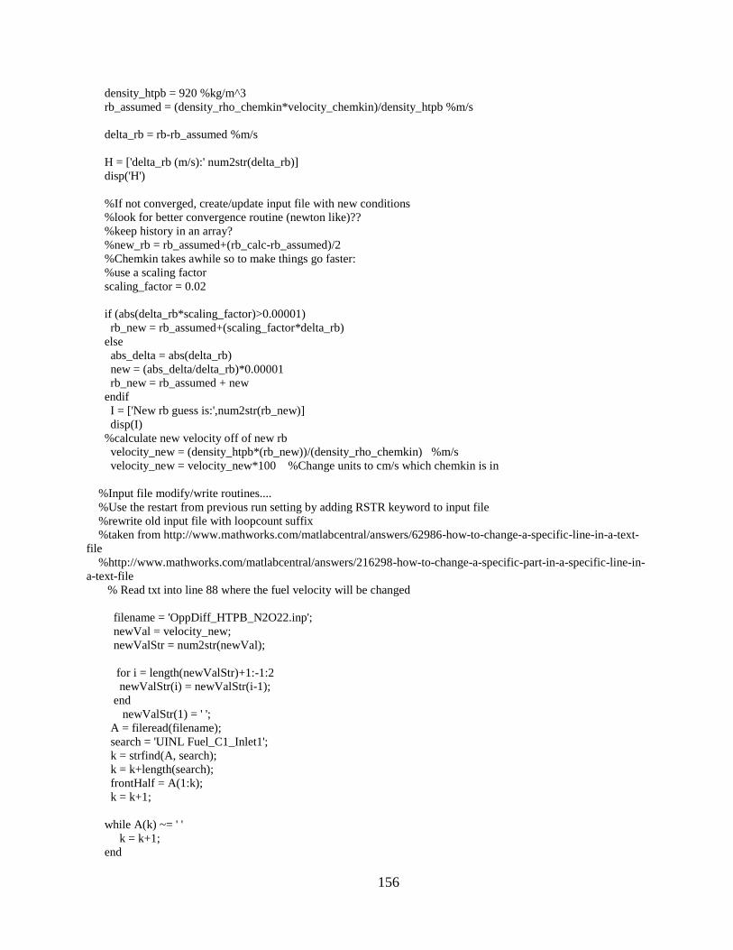
156

density_htpb = 920 %kg/m^3

rb_assumed = (density_rho_chemkin*velocity_chemkin)/density_htpb %m/s

delta_rb = rb-rb_assumed %m/s

H = ['delta_rb (m/s):' num2str(delta_rb)]

disp('H')

%If not converged, create/update input file with new conditions

%look for better convergence routine (newton like)??

%keep history in an array?

%new_rb = rb_assumed+(rb_calc-rb_assumed)/2

%Chemkin takes awhile so to make things go faster:

%use a scaling factor

scaling_factor = 0.02

if (abs(delta_rb*scaling_factor)>0.00001)

rb_new = rb_assumed+(scaling_factor*delta_rb)

else

abs_delta = abs(delta_rb)

new = (abs_delta/delta_rb)*0.00001

rb_new = rb_assumed + new

endif

I = ['New rb guess is:',num2str(rb_new)]

disp(I)

%calculate new velocity off of new rb

velocity_new = (density_htpb*(rb_new))/(density_rho_chemkin) %m/s

velocity_new = velocity_new*100 %Change units to cm/s which chemkin is in

%Input file modify/write routines....

%Use the restart from previous run setting by adding RSTR keyword to input file

%rewrite old input file with loopcount suffix

%taken from http://www.mathworks.com/matlabcentral/answers/62986-how-to-change-a-specific-line-in-a-text-

file

%http://www.mathworks.com/matlabcentral/answers/216298-how-to-change-a-specific-part-in-a-specific-line-in-

a-text-file

% Read txt into line 88 where the fuel velocity will be changed

filename = 'OppDiff_HTPB_N2O22.inp';

newVal = velocity_new;

newValStr = num2str(newVal);

for i = length(newValStr)+1:-1:2

newValStr(i) = newValStr(i-1);

end

newValStr(1) = ' ';

A = fileread(filename);

search = 'UINL Fuel_C1_Inlet1';

k = strfind(A, search);

k = k+length(search);

frontHalf = A(1:k);

k = k+1;

while A(k) ~= ' '

k = k+1;

end

157

backHalf = A(k:end);

A = strcat(frontHalf, newValStr, backHalf)

fileID = fopen(filename, 'w');

fwrite(fileID, A);

fclose(fileID);

%Determine situation and write out final status/results

disp('convergence satisfied')

Pressure = csvread('CKSoln_solution_no_1_1.csv','C2..C2') %dyne/cm^2

Pressure = Pressure*0.1 %Convert dyne/cm^2 to pa 1dyne/cm^2 = 1Pa

Pressure2 = Pressure*1e-6 %convert to megapascals

P = ['Pressure (Pa):', num2str(Pressure)]

A = ['Pressure (MPa):', num2str(Pressure2)]

R = ['Regression rate:' num2str(rb_new)]

Z = ['Delta_Rb:' num2str(delta_rb)]

disp(P)

disp(A)

disp(R)

disp('see chemkin output for details')

disp('hit <enter> to end')

loopcount= loopcount+1 %add this at the end so it actually iterates on the

%on the loopcount and doesn't do it before the

%actual for loop

endwhile

%Now to plot all the solutions!

%First obtain all the information and data using csvread

Temp = csvread('CKSoln_solution_no_1_1.csv', 'K2..K333'); %K

dist = csvread('CKSoln_solution_no_1_1.csv', 'A2..A333'); %cm

heat_release = csvread('CKSoln_solution_no_1_1.csv', 'B2..B333'); %erg/cm^3*sec

heat_release = heat_release*0.1; %convert to J/m^3*s

velocity = csvread('CKSoln_solution_no_1_1.csv', 'M2..M333'); %cm/sec

%mole fractions of species

CO = csvread('CKSoln_solution_no_1_1.csv', 'O2..O333');

CO2 = csvread('CKSoln_solution_no_1_1.csv', 'P2..P333');

NO = csvread('CKSoln_solution_no_1_1.csv', 'Q2..Q333');

H = csvread('CKSoln_solution_no_1_1.csv', 'S2..S333');

H2 = csvread('CKSoln_solution_no_1_1.csv', 'X2..X333');

O = csvread('CKSoln_solution_no_1_1.csv', 'T2..T333');

OH = csvread('CKSoln_solution_no_1_1.csv', 'U2..U333');

O2 = csvread('CKSoln_solution_no_1_1.csv', 'W2..W333');

H2O = csvread('CKSoln_solution_no_1_1.csv', 'Z2..Z333');

C = csvread('CKSoln_solution_no_1_1.csv', 'AH2..AH333');

C2H4 = csvread('CKSoln_solution_no_1_1.csv', 'AN2..AN333');

N = csvread('CKSoln_solution_no_1_1.csv', 'BL2..BL333');

N2O = csvread('CKSoln_solution_no_1_1.csv', 'BO2..BO333');

CN = csvread('CKSoln_solution_no_1_1.csv', 'BP2..BP333');

%Now plot results using plot

158

figure(1);

plot(dist,C2H4, dist,O2, dist, CO, dist, H2O, dist, H2, dist, CO2, dist, N2O, dist, NO);

title(['Mole fractions for ',num2str(Pressure2), 'MPa']);

xlabel('Distance (cm)');

ylabel('Mole Fractions ()');

axis([0,0.5,0,1])

legend('C2H4','O2','CO','H2O','H2','CO2','N2O','NO');

figure(2);

plot(dist,Temp*1e6, dist, heat_release);

title(['Temperature and Heat Release Rate for ',num2str(Pressure2),'MPa']);

xlabel('Distance (cm)');

ylabel('Temperature (K) and Heat Release Rate (erg/cm^3*sec)');

axis([0,0.5,-1e+10,2e+10])

legend('Temperature X 1E6', 'Heat Release Rate');

Subroutines to Follow:

## Author: PKN5018 <PKN5018@MNE-HPCL21>

## Created: 2015-12-04

function [delta_h] = Find_delta_sensible_enthalpy (Ti, Tf)

%Find sensible enthalpy difference in gas C2H4 between two temps by using

%finding integral of CpdT of gas C2H4

MW = 28.05 %g/mol

MW2 = MW*1000 %g/kmol

%DIPPR Coefficients for ideal gas heat capacity

A = 3.338e4

B = 9.479e4

C = 1.596e3

D = 5.51e4

E = 7.408e2

%DIPPRR coefficients for liquid heat capacity

%A = 2.4739e560<

%B = -4.428e3

%C = 4.0936e1

%D = -1.697e-1

%E = 2.6816e-4

%DIPRR Cp values good for 60<T<1500 for ideal gas

if Ti>1500 %K

disp('Warning initial temperature for liquid sensible enthalpy (Cp_fit) out of range')

endif

if Tf>1500 %K

disp('Warning final temperature for liquid sensible enthalpy (Cp_fit) out of range')

endif

%DIPRR Cp values good for 104<T<252.7 for liquid

%if Ti>252.7 %K

%disp('Warning initial temperature for liquid sensible enthalpy (Cp_fit) out of range')

%endif

%if Tf>252.7 %K

%disp('Warning final temperature for liquid sensible enthalpy (Cp_fit) out of range')

%endif

159

%DIPRR Cp curve fit: Equation 100 for ideal gas

%A+B*[(C/T)/sinh(C/T)]^2+D*[(E/T)/cosh(E/T)]^2

%Integrate polynomial to get A*T + B*C*coth(C/T)-D*E*tanh(E/T) used wolframalpha to get integral

h_final = A*Tf+B*C*coth(C/Tf)-D*E*tanh(E/Tf)

h_initial = A*Ti+B*C*coth(C/Ti)-D*E*tanh(E/Ti)

%DIPRR Cp curve fit: Equation 100 for liquid

%A+(B*T) + (C*T^2)+(D*T^3)+(E*T^4)

%Integrate polynomial to get A*T+ 1/2(B*T^2) + (C/3)*T^3 + (D/4)*T^4 + (E/5)*T^5

%h_final = A*Tf+(B/2)*Tf^2+(C/3)*Tf^3+(D/4)*Tf^4+(E/5)*Tf^5

%h_initial = A*Tf+(B/2)*Tf^2+(C/3)*Tf^3+(D/4)*Ti^4+(E/5)*Ti^5

molar_delta_h = h_final-h_initial

%integrated DIRPR Cp yields J/kmol so convert to J/g

delta_h = (molar_delta_h/MW2) %J/g

U = ['delta_h', num2str(delta_h)]

Endfunction

function [qr] = Find_Heat_of_Reaction (Ts)

%Find heat of vapoization of liquid C2H4 at given surface temperautre in..

%Calculate liquid Cp for C2H4 as a function of T based on DIPRR fit

%C2H4 critical properties

MW = 28.05 %kg/kmol for C2H4

MW2 = 26.03728 %kg/kmol for C2H2

MW3 = (MW2+MW)/2

Tcrit = 282.34 %K http://encyclopedia.airliquide.com/encyclopedia.asp?GasID=29#MajorApplications

%DIPRR is down and connot find coefficients so use Dr. Boyers for right now

%DIPRR values good for 102 to 282.34 K

%if Ts > 282.34

%disp('Warning: Temperature for heat of vaporization out of range')

%endif

%DIPRR coefficients

%A = 2.0639e7

%B = 8.0135e-1

%C = -8.128e-1

%D = 4.179e-1

%DIPRR says there is an E in the equation but not in the coefficients.....

%Calculate reduced temperature

%Tr = Ts/Tcrit

%DIPRR curve fit eqn 106

%e = B+C*Tr+D*Tr^2

%molar_Lvap = A*(1-Tr)^e %J/kmol

%DIPRR proerty given in J/KMOL, so divide by molecular weight of C2H4 and

%convert to J/g to get in energy/mass units

%Lvap = (molar_Lvap/MW)/1000 %J/g

%L = ['Lvap:', num2str(Lvap)]

%disp(L)

%Determine Heat of Reaction since it goes from solid to gas due to qr

160

%C7.337+H10.982 <--> XC2H4+j*C2H2

%Do a stiochiometric eqn and solve it

x = 1.83425

j = 1.83425 %Added C2H2 instead to conserve C

%Now that the stiochiometric coefficients are solved for solve for the qr

%qr = Hproducts-Hreactants

%Products at Ts of 600K may have to change depending on the temperature you need

deltaH_C2H2 = 15.771 %KJ/mol

Hf_C2H2 = 216.993 %KJ/mol

deltaH_C2H4 = 17.335 %KJ/mol

Hf_C2H4 = 44.294 %KJ/mol

%deltaH_O2 = 9.244 %KJ/mol

%deltaH_N2 = 8.894 %KJ/mol

%Hf_CO = 8.942 %added in to see if it changed anything based upon a non balance of values for HTPB to C2H4

%deltaH_CO = -110.15 %added in to see if it changed anythign

%Reactants at Tr of 298K

%Hf_N2O = 82.05 %KJ/mol http://webbook.nist.gov/cgi/cbook.cgi?ID=C10024972&Mask=1

Hf_HTPB = -51.8 %KJ/mol http://www.lr.tudelft.nl/en/organisation/departments/space-engineering/space-systems-

engineering/expertise-areas/space-propulsion/design-of-elements/rocket-propellants/solids/physical-properties/

Hproducts = (x*(deltaH_C2H4+Hf_C2H4)+j*(deltaH_C2H2+Hf_C2H2))

Hreactants = Hf_HTPB

qr_molar = Hproducts-Hreactants %in KJ/mol

MW_HTPB = 138 %g/mol

%Should I use MW_HTPB or MW of C2H4??

qr = (qr_molar/MW_HTPB)*1000 %J/g

Q = ['Heat of reaction: J/g', num2str(qr)]

disp(Q)

%heat of formation for HTPB and N2O is in the Rocket Propulsion elements book on page 583!!!!!!

Endfunction

function [k] = Find_k (T_ave)

%Find thermal conductivity of gas at given temperature in W/m-K

%DIPPR coefficients from http://dippr.byu.edu/public/chemsearch.asp?Mode=Printout2&ChemID=201

%DIPRR coefficients for C2H4 right now since that is the gasous fuel

%A = 8.6806e-6

%B = 1.4559

%C = 2.9972E2

%D = -2.9403e4

%for testing, use an approximate constant value ***fixme***

%k = 2e-2 %W/m-K

%Once working calculate k for C2H4 as a function of T based on DIPPR fit

%DIPPR values good for 170K to 590K

%if T_ave>590

%disp('Warning temperature for thermal conductivity (k) fit out of range')

%endif

161

%DIPRR curve fit: http://dippr.byu.edu/public/calculator.asp?ChemID=201&PropertyID=VTC&SetOrder=A

%k = (A*T_ave^B)/((1+(C/T_ave)+(D/T_ave^2))) %W/m*K

%DIPRR properties in W/m*K

f1 = csvread('CKSoln_solution_no_1.csv', 'E2..E2') %Erg/cm*K*s

f2 = csvread('CKSoln_solution_no_1.csv', 'E3..E3') %Erg/cm*K*s

f = (f1+f2)/2

k = f*1E-7 %W/m*K

K = ['thermal conductivity K=(W/m*K)',num2str(k)]

disp(K)

endfunction

function [rb] = Find_rb (dTdx, Ts, Ti, T_ave, Tf)

[k] = Find_k (T_ave)

[qr] = Find_Heat_of_Reaction (Ts)

[rho_gas] = Find_rho_gas(Ti)

[delta_h] = Find_delta_sensible_enthalpy(Ti,Tf)

q = k*dTdx %J/s*m^2

%Find Evaporation flux based on heat flux (vaporization)

m_flux_gassification = q/(delta_h-qr) %Check units g/s*m^2

%for CHEMKIN, need mass flux in g/cm^2*s

%check units on preperty lookup subroutines

%---> use modot times desnity (DIPPR lookup at initial

rb = abs(m_flux_gassification/rho_gas) %Check units should be m/s

endfunction

function [rho_gas] = Find_rho_gas (Ts)

%Find density of liquid of C2H4 at given surface temperature in g/cm^3

MW = 28.05 %g/mol for C2H4

MW2 = 26.04 %g/mol for C2H2

MW3 = (MW+MW2)/2

%calculate liquid density for C2H4 as a function of T based on DIPRR fit

%DIPRR coefficients

%A = 2.0961

%B = 2.7657e-1

%C = 2.8234e2

%D = 2.9147e-1

%Temperature range for eqn 104K<T<282.34K

%Liquid density DIPRR eqn from eqn 105

%e2 = 1+(1-Ts/C)^D

%rho_liquid = A/ (B^e2)

%for testing, use an approximate constant value

Pressure = csvread('CKSoln_solution_no_1_1.csv','C2..C2') %dyne/cm^2

Pressure = Pressure*0.1 %Convert dyne/cm^2 to pa 1dyne/cm^2 = 1Pa

Ru = 8314 %J/kmol*K

R = Ru/MW3 %J/kg*K

rho_gas = Pressure/(R*Ts) %kg/m^3

rho_gas = rho_gas*1000 %g/m^3

162

%Find rho_gas based upon Ideal Gas Law

Endfunction

function [N, R, Q, F] = Set_CHEMKIN_env ()

% Establish the CHEMKIN environment (see section 4.1.2 in "Getting Started")

% Open a DOS window and type set in the DOS window

% Use setenv to set environment values and getenv retreives the value specfied in

% the setenv

%Set REACTION_DIR = C:\Program Files\Reaction

%Set CHEMKIN_VERS=10141

%Set CHEMKIN_BIN = C:\Program Files\Reaction\chemkin15141_win64\bin

%Set CHEMKIN_RELEASE_NUMBER = 10141 <x64> (08 Jul 2015)

%Set shell environment variables

setenv('REACTION_DIR','"C:\Program Files\Reaction"');

N = getenv('REACTION_DIR');

setenv('CHEMKIN_VERS=15151');

R = getenv('CHEMKIN_VERS');

setenv('CHEMKIN_BIN','"C:\Program Files\Reaction\chemkin15151_win64\bin"');

Q = getenv('CHEMKIN_BIN');

setenv('CHEMKIN_RELEASE_NUMBER=Release_15151 <x64> (18 Jan 2016)');

F = getenv('CHEMKIN_RELEASE_NUMBER');

%Set PATH to include CHEMKIN binary directory

S = 'CHEMKIN environment set.'

disp(S)

endfunction

function [cmdout4] = Run_shell (shell_cmd)

[shell_result, cmdout4] = system(shell_cmd)

%if (shell_result==1)

%shell_err = ierrno( )

%disp('Error')

%disp('Error trying to execute the following shell command.')

%endif

endfunction

163

Appendix G: Transport Input Data

!***********************************************************************BEGIN-HDR

!

! Copyright (c) 1997-2006 Reaction Design. All rights reserved.

!

! $Header: /chemkin/4.2/prebuild/data/tran.dat 8 12/21/06 9:20a Frupley $

!

! $NoKeywords: $

!***********************************************************************END-HDR

AR 0 136.500 3.330 0.000 0.000 0.000

AR* 0 136.500 3.330 0.000 0.000 0.000

C 0 71.400 3.298 0.000 0.000 0.000 !(*)

C2 1 97.530 3.621 0.000 1.760 4.000

C2O 1 232.400 3.828 0.000 0.000 1.000 ! *

CN2 1 232.400 3.828 0.000 0.000 1.000 ! OIS

C2H 1 209.000 4.100 0.000 0.000 2.500

C2H2 1 209.000 4.100 0.000 0.000 2.500

C2H2OH 2 224.700 4.162 0.000 0.000 1.000 !(*)

CH2OH 2 417.000 3.690 1.700 0.000 2.000

C2H3 2 209.000 4.100 0.000 0.000 1.000 !(*)

C2H4 2 280.800 3.971 0.000 0.000 1.500

C2H5 2 252.300 4.302 0.000 0.000 1.500

C2H6 2 252.300 4.302 0.000 0.000 1.500

C2N 1 232.400 3.828 0.000 0.000 1.000 ! OIS

C2N2 1 349.000 4.361 0.000 0.000 1.000 !(OIS)

C3H2 2 209.000 4.100 0.000 0.000 1.000 !(*)

C3H3 1 252.000 4.760 0.000 0.000 1.000

C3H4 1 252.000 4.760 0.000 0.000 1.000

C3H4P 1 252.000 4.760 0.000 0.000 1.000 ! JAM

C3H6 2 266.800 4.982 0.000 0.000 1.000

C3H7 2 266.800 4.982 0.000 0.000 1.000

C4H6 2 357.000 5.180 0.000 0.000 1.000

I*C3H7 2 266.800 4.982 0.000 0.000 1.000

N*C3H7 2 266.800 4.982 0.000 0.000 1.000

C3H8 2 266.800 4.982 0.000 0.000 1.000

C4H 1 357.000 5.180 0.000 0.000 1.000

C4H2 1 357.000 5.180 0.000 0.000 1.000

C4H2OH 2 224.700 4.162 0.000 0.000 1.000 !(*)

C4H3 1 357.000 5.180 0.000 0.000 1.000

C4H4 1 357.000 5.180 0.000 0.000 1.000

C4H8 2 357.000 5.176 0.000 0.000 1.000

C4H9 2 357.000 5.176 0.000 0.000 1.000

S*C4H9 2 357.000 5.176 0.000 0.000 1.000

C4H9 2 357.000 5.176 0.000 0.000 1.000

I*C4H9 2 357.000 5.176 0.000 0.000 1.000

C5H2 1 357.000 5.180 0.000 0.000 1.000

C5H3 1 357.000 5.180 0.000 0.000 1.000

C6H2 1 357.000 5.180 0.000 0.000 1.000

C6H5 2 412.300 5.349 0.000 0.000 1.000 ! JAM

C6H5(L) 2 412.300 5.349 0.000 0.000 1.000 ! JAM

C6H5O 2 450.000 5.500 0.000 0.000 1.000 ! JAM

C5H5OH 2 450.000 5.500 0.000 0.000 1.000 ! JAM

C6H6 2 412.300 5.349 0.000 0.000 1.000 ! SVE

C6H7 2 412.300 5.349 0.000 0.000 1.000 ! JAM

CH 1 80.000 2.750 0.000 0.000 0.000

CH2 1 144.000 3.800 0.000 0.000 0.000

CH2(S) 1 144.000 3.800 0.000 0.000 0.000

CH2(SING) 1 144.000 3.800 0.000 0.000 0.000

CH2CHCCH 2 357.000 5.180 0.000 0.000 1.000 ! JAM

CH2CHCCH2 2 357.000 5.180 0.000 0.000 1.000 ! JAM

CH2CHCH2 2 260.000 4.850 0.000 0.000 1.000 ! JAM

164

CH2CHCHCH 2 357.000 5.180 0.000 0.000 1.000 ! JAM

CH2CHCHCH2 2 357.000 5.180 0.000 0.000 1.000 ! JAM

CH2CO 2 436.000 3.970 0.000 0.000 2.000

CH2O 2 498.000 3.590 0.000 0.000 2.000

CH3 1 144.000 3.800 0.000 0.000 0.000

CH3CC 2 252.000 4.760 0.000 0.000 1.000 ! JAM

CH3CCCH2 2 357.000 5.180 0.000 0.000 1.000 ! JAM

CH3CCCH3 2 357.000 5.180 0.000 0.000 1.000 ! JAM

CH3CCH2 2 260.000 4.850 0.000 0.000 1.000 ! JAM

CH3CHCH 2 260.000 4.850 0.000 0.000 1.000 ! JAM

CH3CH2CCH 2 357.000 5.180 0.000 0.000 1.000 ! JAM

CH3CHO 2 436.000 3.970 0.000 0.000 2.000

CH3CO 2 436.000 3.970 0.000 0.000 2.000

CH3O 2 417.000 3.690 1.700 0.000 2.000

CH3OH 2 481.800 3.626 0.000 0.000 1.000 ! SVE

CH3HCO 2 436.000 3.970 0.000 0.000 2.000 ! Added myself for

transport data needed for program

OCHCHO 2 406.937 4.823 0.000 0.000 2.000 ! Added myself for

transport data needed for program

C2H5CHO 2 435.200 4.662 2.700 0.000 1.000 ! Added myself for

transport data needed for progrm

C2H5CO 2 424.600 4.820 0.000 0.000 1.000 ! Added myself for


NO3 2 200.000 3.500 0.000 0.000 1.000 ! Added myself for


HONO 2 232.400 3.828 0.000 0.000 1.000 ! Added myself for


CH3CN 2 436.000 3.970 0.000 0.000 2.000 ! Added myself for


CH2CN 2 436.000 3.970 0.000 0.000 2.000 ! Added myself for


CH4 2 141.400 3.746 0.000 2.600 13.000

CH4O 2 417.000 3.690 1.700 0.000 2.000

CN 1 75.000 3.856 0.000 0.000 1.000 !(OIS)

CNC 1 232.400 3.828 0.000 0.000 1.000 ! OIS

CNN 1 232.400 3.828 0.000 0.000 1.000 ! OIS

CO 1 98.100 3.650 0.000 1.950 1.800

CO2 1 244.000 3.763 0.000 2.650 2.100

CL 0 130.8 3.613 0.000 0.000 1.000 !(singh)

CL- 0 130.8 3.613 0.000 0.000 1.000 !(singh)

E 0 850. 425. 0.000 0.000 1.000 !(singh)

F 0 80.000 2.750 0.000 0.000 0.000

F2 1 125.700 3.301 0.000 1.600 3.800

H 0 145.000 2.050 0.000 0.000 0.000

H2C4O 2 357.000 5.180 0.000 0.000 1.000 ! JAM

H2 1 38.000 2.920 0.000 0.790 280.000

H2CCCCH 2 357.000 5.180 0.000 0.000 1.000 ! JAM

H2CCCCH2 2 357.000 5.180 0.000 0.000 1.000 ! JAM

H2CCCH 2 252.000 4.760 0.000 0.000 1.000 ! JAM

H2CN 1 569.000 3.630 0.000 0.000 1.000 ! os/jm

H2NO 2 116.700 3.492 0.000 0.000 1.000 ! JAM

H2O 2 572.400 2.605 1.844 0.000 4.000

H2O2 2 107.400 3.458 0.000 0.000 3.800

H2S 2 301.000 3.600 0.000 0.000 1.000 !(OIS)

HC2N2 1 349.000 4.361 0.000 0.000 1.000 ! OIS

HCCHCCH 2 357.000 5.180 0.000 0.000 1.000 ! JAM

HCCO 2 150.000 2.500 0.000 0.000 1.000 !(*)

HCCOH 2 436.000 3.970 0.000 0.000 2.000

HCN 1 569.000 3.630 0.000 0.000 1.000 !(OIS)

HCNO 2 232.400 3.828 0.000 0.000 1.000 ! JAM

HCO 2 498.000 3.590 0.000 0.000 0.000

HCO+ 1 498.000 3.590 0.000 0.000 0.000

HCL 1 344.7 3.339 0.000 0.000 1.000 !(singh)

165

HF 1 330.000 3.148 1.920 2.460 1.000 ! sv/mec

HF0 1 352.000 2.490 1.730 0.000 5.000

HF1 1 352.000 2.490 1.730 0.000 5.000

HF2 1 352.000 2.490 1.730 0.000 5.000

HF3 1 352.000 2.490 1.730 0.000 5.000

HF4 1 352.000 2.490 1.730 0.000 5.000

HF5 1 352.000 2.490 1.730 0.000 5.000

HF6 1 352.000 2.490 1.730 0.000 5.000

HF7 1 352.000 2.490 1.730 0.000 5.000

HF8 1 352.000 2.490 1.730 0.000 5.000

CH2HCO 2 436.000 3.970 0.000 0.000 2.000

HOCN 2 232.400 3.828 0.000 0.000 1.000 !(JAM)

HNCO 2 232.400 3.828 0.000 0.000 1.000 !(OIS)

HNNO 2 232.400 3.828 0.000 0.000 1.000 !(*)

HNO 2 116.700 3.492 0.000 0.000 1.000 !(*)

HNOH 2 116.700 3.492 0.000 0.000 1.000 ! JAM

HO2 2 107.400 3.458 0.000 0.000 1.000 !(*)

HSO2 2 252.000 4.290 0.000 0.000 1.000 !(OIS)

HE 0 10.200 2.576 0.000 0.000 0.000 !(*)

K 0 850. 4.25 0.000 0.000 1.000 !(singh)

KCL 1 1989. 4.186 0.000 0.000 1.000 !(singh)

KO 1 383.0 3.812 0.000 0.000 1.000 !(singh)

KOH 2 1213. 4.52 0.000 0.000 1.000 !(singh)

KO2 2 1213. 4.69 0.000 0.000 1.000 !(singh)

KH 1 93.3 3.542 0.000 0.000 1.000 !(singh)

K+ 0 850. 4.25 0.000 0.000 1.000 !(singh)

N 0 71.400 3.298 0.000 0.000 0.000 !(*)

N2 1 97.530 3.621 0.000 1.760 4.000

N2H2 2 71.400 3.798 0.000 0.000 1.000 !(*)

N2H3 2 200.000 3.900 0.000 0.000 1.000 !(*)

N2H4 2 205.000 4.230 0.000 4.260 1.500

N2O 1 232.400 3.828 0.000 0.000 1.000 !(*)

NCN 1 232.400 3.828 0.000 0.000 1.000 ! OIS

NCO 1 232.400 3.828 0.000 0.000 1.000 !(OIS)

NH 1 80.000 2.650 0.000 0.000 4.000

NH2 2 80.000 2.650 0.000 2.260 4.000

NH3 2 481.000 2.920 1.470 0.000 10.000

NNH 2 71.400 3.798 0.000 0.000 1.000 !(*)

NO 1 97.530 3.621 0.000 1.760 4.000

NCNO 2 232.400 3.828 0.000 0.000 1.000 ! OIS

NO2 2 200.000 3.500 0.000 0.000 1.000 !(*)

O 0 80.000 2.750 0.000 0.000 0.000

O2 1 107.400 3.458 0.000 1.600 3.800

O3 2 180.000 4.100 0.000 0.000 2.000

OH 1 80.000 2.750 0.000 0.000 0.000

S 0 847.000 3.839 0.000 0.000 0.000 !(OIS)

S2 1 847.000 3.900 0.000 0.000 1.000 !(OIS)

SH 1 847.000 3.900 0.000 0.000 1.000 !(OIS)

SO 1 301.000 3.993 0.000 0.000 1.000 !(OIS)

SO2 2 252.000 4.290 0.000 0.000 1.000 !(OIS)

SO3 2 378.400 4.175 0.000 0.000 1.000 !(OIS)

!

! Local Additions for Silicon CVD

!

H2SISIH2 2 312.6 4.601 0.000 0.000 1.000 !(mec)

H3SISIH 2 312.6 4.601 0.000 0.000 1.000 !(mec)

SI 0 3036. 2.910 0.000 0.000 0.000 !(mec)

SIH 1 95.8 3.662 0.000 0.000 1.000 !(mec)

SIH2 2 133.1 3.803 0.000 0.000 1.000 !(mec)

SIH2(3) 2 133.1 3.803 0.000 0.000 1.000 !(mec)

SIH3 2 170.3 3.943 0.000 0.000 1.000 !(mec)

SIH4 2 207.6 4.084 0.000 0.000 1.000 !(mec)

SI2 1 3036. 3.280 0.000 0.000 1.000 !(mec)

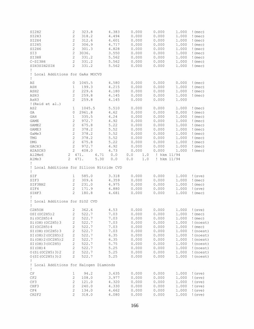
166

SI2H2 2 323.8 4.383 0.000 0.000 1.000 !(mec)

SI2H3 2 318.2 4.494 0.000 0.000 1.000 !(mec)

SI2H4 2 312.6 4.601 0.000 0.000 1.000 !(mec)

SI2H5 2 306.9 4.717 0.000 0.000 1.000 !(mec)

SI2H6 2 301.3 4.828 0.000 0.000 1.000 !(mec)

SI3 2 3036. 3.550 0.000 0.000 1.000 !(mec)

SI3H8 2 331.2 5.562 0.000 0.000 1.000 !(mec)

C-SI3H6 2 331.2 5.562 0.000 0.000 1.000 !(mec)

SIH3SIH2SIH 2 331.2 5.562 0.000 0.000 1.000 !(mec)

!

! Local Additions for GaAs MOCVD

!

AS 0 1045.5 4.580 0.000 0.000 0.000 !(mec)

ASH 1 199.3 4.215 0.000 0.000 1.000 !(mec)

ASH2 2 229.6 4.180 0.000 0.000 1.000 !(mec)

ASH3 2 259.8 4.145 0.000 0.000 1.000 !(mec)

AsH3 2 259.8 4.145 0.000 0.000 1.000

!(Reid et al.)

AS2 1 1045.5 5.510 0.000 0.000 1.000 !(mec)

GA 0 2961.8 4.62 0.000 0.000 0.000 !(mec)

GAH 1 335.5 4.24 0.000 0.000 1.000 !(mec)

GAME 2 972.7 4.92 0.000 0.000 1.000 !(mec)

GAME2 2 675.8 5.22 0.000 0.000 1.000 !(mec)

GAME3 2 378.2 5.52 0.000 0.000 1.000 !(mec)

GaMe3 2 378.2 5.52 0.000 0.000 1.000 !(mec)

TMG 2 378.2 5.52 0.000 0.000 1.000 !(mec)

DMG 2 675.8 5.22 0.000 0.000 1.000 !(mec)

GACH3 2 972.7 4.92 0.000 0.000 1.000 !(mec)

H2ASCH3 2 408.0 4.73 0.000 0.000 1.000 !(mec)

Al2Me6 2 471. 6.71 0.0 0.0 1.0 ! hkm 11/94

AlMe3 2 471. 5.30 0.0 0.0 1.0 ! hkm 11/94

!

! Local Additions for Silicon Nitride CVD

!

SIF 1 585.0 3.318 0.000 0.000 1.000 !(sve)

SIF3 2 309.6 4.359 0.000 0.000 1.000 !(mec)

SIF3NH2 2 231.0 4.975 0.000 0.000 1.000 !(mec)

SIF4 2 171.9 4.880 0.000 0.000 1.000 !(sve)

SIHF3 2 180.8 4.681 0.000 0.000 1.000 !(mec)

!

! Local Additions for SiO2 CVD

!

C2H5OH 2 362.6 4.53 0.000 0.000 1.000 !(sve)

OSI(OC2H5)2 2 522.7 7.03 0.000 0.000 1.000 !(mec)

Si(OC2H5)4 2 522.7 7.03 0.000 0.000 1.000 !(mec)

Si(OH)(OC2H5)3 2 522.7 7.03 0.000 0.000 1.000 !(noest)

SI(OC2H5)4 2 522.7 7.03 0.000 0.000 1.000 !(mec)

SI(OH)(OC2H5)3 2 522.7 7.03 0.000 0.000 1.000 !(noest)

SI(OH)2(OC2H5)2 2 522.7 6.35 0.000 0.000 1.000 !(noest)

Si(OH)2(OC2H5)2 2 522.7 6.35 0.000 0.000 1.000 !(noest)

SI(OH)3(OC2H5) 2 522.7 5.75 0.000 0.000 1.000 !(noest)

SI(OH)4 2 522.7 5.25 0.000 0.000 1.000 !(noest)

O(Si(OC2H5)3)2 2 522.7 5.25 0.000 0.000 1.000 !(noest)

O(SI(OC2H5)3)2 2 522.7 5.25 0.000 0.000 1.000 !(noest)

!

! Local Additions for Halogen Diamonds

!

CF 1 94.2 3.635 0.000 0.000 1.000 !(sve)

CF2 2 108.0 3.977 0.000 0.000 1.000 !(sve)

CF3 2 121.0 4.320 0.000 0.000 1.000 !(sve)

CHF3 2 240.0 4.330 0.000 0.000 1.000 !(sve)

CF4 2 134.0 4.662 0.000 0.000 1.000 !(sve)

CH2F2 2 318.0 4.080 0.000 0.000 1.000 !(sve)

167

C2F4 2 202.6 5.164 0.000 0.000 1.000 !(mec)

C2F6 2 194.5 5.512 0.000 0.000 1.000 !(mec)

! New entries for In, InMe3, PH3, InAsMe

PH3 2 251.5 3.981 0.000 0.000 1.000

!(Reid et al.)

BCL3 2 337.7 5.127 0.000 0.000 1.000 !svehla

CL2BNH2 2 337.7 5.127 0.000 0.000 1.000

!mec guess

168

Appendix H: Calibrations

Pressure Transducer

The pressure transducers that were used in the motor and opposed flow burner studies

were Setra Model 206 (Industrial Pressure Transducer) transducers. These were chosen based

upon the high performance, reliability, versatility and ability to record 1000 Hz for a longer time

span. The pressure ranges of the transducers used was 0-1000 psig to 0-3000 psig. To calibrate

the transducer, a gauge calibration box was used. Inert gas was supplied to the gauge box with

the pressure transducer connected to it as well. An excitation voltage was supplied while a BNC

cable obtained the voltage output of the transducer. Pressure was supplied with increments of 50

psig up to a level given the range of the Setra. Afterwards a linear fit was applied to get an

equation correlating voltage to a given pressure.

Choked Flow of Fuel and Ideal Gas

When conducting experiments with the opposed flow burner using N2O oxidizer, the

apparatus enters supercritical conditions. Unfortunately these conditions that were seen when

using the counterflow burner are above the critical temperature and most likely pressure, where

N2O begins to deviate from the ideal gas law (becoming non-linear with the dependence of

density on pressure). Therefore, the choked flow equations used to obtain a mass flow rate can

no longer be used, so an empirical equation was generated as a function of upstream pressure and

orifice diameter. This was accomplished by recording the upstream pressure and mass flow rate

downstream with a bubble meter. This was done for two different orifice sizes, generating a

polynomial fit to the normalized flow rate. A polynomial was then generated for mass flow rate

as a function of upstream pressure for each orifice. The results are shown in Figure H.1 and the

empirical equation provided in Eq. H.1.

169

�̇� = 17.98𝑃2 + 276.17𝑃 + 16.188 (H.1)

where the mass flow is in g/s and P is in MPa.

Figure H.1: Empirical fits for normalized N2O mass flow rates.

diffusion flame stuides of solid fuels with nitrous …

Documents