RESEARCH ARTICLE Open Access

Difficulty in inferring microbial communitystructure based on co-occurrence networkapproachesHokuto Hirano and Kazuhiro Takemoto*

Abstract

Background: Co-occurrence networks—ecological associations between sampled populations of microbialcommunities inferred from taxonomic composition data obtained from high-throughput sequencing techniques—are widely used in microbial ecology. Several co-occurrence network methods have been proposed. Co-occurrencenetwork methods only infer ecological associations and are often used to discuss species interactions. However,validity of this application of co-occurrence network methods is currently debated. In particular, they simplyevaluate using parametric statistical models, even though microbial compositions are determined throughpopulation dynamics.

Results: We comprehensively evaluated the validity of common methods for inferring microbial ecologicalnetworks through realistic simulations. We evaluated how correctly nine widely used methods describe interactionpatterns in ecological communities. Contrary to previous studies, the performance of the co-occurrence networkmethods on compositional data was almost equal to or less than that of classical methods (e.g., Pearson’scorrelation). The methods described the interaction patterns in dense and/or heterogeneous networks ratherinadequately. Co-occurrence network performance also depended upon interaction types; specifically, theinteraction patterns in competitive communities were relatively accurately predicted while those in predator–prey(parasitic) communities were relatively inadequately predicted.

Conclusions: Our findings indicated that co-occurrence network approaches may be insufficient in interpretingspecies interactions in microbiome studies. However, the results do not diminish the importance of theseapproaches. Rather, they highlight the need for further careful evaluation of the validity of these much-usedmethods and the development of more suitable methods for inferring microbial ecological networks.

Keywords: Microbiome, Correlation network analysis, Microbial ecology, Complex networks

BackgroundMany microbes engage with one another through inter-specific interactions (e.g., mutualistic and competitive in-teractions) to compose ecological communities andinterrelate with their surrounding environments (e.g., theirhosts) [1]. Investigating such communities is importantnot only in the context of basic scientific research [2, 3],but also in applied biological research fields, such as inmedical [4] and environmental sciences [5]. Remarkabledevelopment of high-throughput sequencing techniques—

e.g., 16S ribosomal RNA gene sequencing and metage-nomics as well as computational pipelines—have providedsnapshots of taxonomic compositions in microbial com-munities across diverse ecosystems [6] and revealed thatmicrobial compositions are associated with human healthand ecological environments. For example, microbialcomposition in the human gut is interrelated with by nu-merous diseases—such as diabetes and cardiovascular dis-ease—age, diet, and antibiotic use [7, 8]. The compositionof soil microbial communities is related to climate, aridity,pH, and plant productivity [9]. However, previous studieshave been limited to the context of species composition,and the effect of the structure of microbial communities(microbial ecological networks) on such associations is

© The Author(s). 2019 Open Access This article is distributed under the terms of the Creative Commons Attribution 4.0International License (http://creativecommons.org/licenses/by/4.0/), which permits unrestricted use, distribution, andreproduction in any medium, provided you give appropriate credit to the original author(s) and the source, provide a link tothe Creative Commons license, and indicate if changes were made. The Creative Commons Public Domain Dedication waiver(http://creativecommons.org/publicdomain/zero/1.0/) applies to the data made available in this article, unless otherwise stated.

* Correspondence: takemoto@bio.kyutech.ac.jpDepartment of Bioscience and Bioinformatics, Kyushu Institute ofTechnology, Iizuka, Fukuoka 820-8502, Japan

Hirano and Takemoto BMC Bioinformatics (2019) 20:329 https://doi.org/10.1186/s12859-019-2915-1

unclear due to a lack of reliable methods through whichreal interaction networks can be captured. Thus, co-occurrence networks, which infer ecological associationsbetween sampled populations of microbial communitiesobtained from high-throughput sequencing techniques,have been attracting attention [10]. Co-occurrence net-work approaches are also related to weighted correlationnetwork analyses [11–13] for inferring molecular net-works from high-throughput experimental data, such asgene expression data. A number of methods for inferringmicrobial association have been proposed.As a simple metric, Pearson’s correlation coefficient is

considered. Additionally, Spearman’s correlation coeffi-cient and maximal information coefficient (MIC) [14]are useful for accurately detecting non-linear associa-tions. However, these metrics may not be applicable tocompositional data because the assumption of independ-ent variables may not be satisfied due to the constant sumconstraint [15]. Particularly, spurious correlations may beobserved when directly applying these metrics to compos-itional data. To avoid this limitation, Sparse Correlationsfor Compositional data (SparCC) [16] has been developed.SparCC is an iterative approximation approach and esti-mates the correlations between the underlying absoluteabundances using the log-ratio transformation of compos-itional data under the assumptions that real-world micro-bial networks are large-scale and sparse. However, SparCCis not efficient due to its high computational complexity.Thus, regularized estimation of the basis covariance basedon compositional data (REBACCA) [17] and correlation in-ference for compositional data through Lasso (CCLasso)[18] have been proposed. These methods are considerablyfaster than SparCC by using the l1-norm shrinkage method(i.e., least absolute shrinkage and selection operator; Lasso).SparCC has further limitations, as it does not consider errorsin compositional data and the inferred covariance matrixmay be not positive definite. To avoid these limitations,CCLasso considers a loss function inspired by the lasso pe-nalized D-trace loss.However, correlation-based approaches such as those men-

tioned above may detect indirect associations. To differentiatedirect and indirect interactions in correlation inference, othermethods have been developed. In this context, inverse covari-ance matrix-based approaches are often used because they es-timate an underlying graphical model, employing the conceptof conditional independence. Typically, Pearson’s and Spear-man’s partial correlation coefficients are used [19]; however,they may be not applicable to compositional data because stat-istical artifacts may occur due to the constant sum constraint.Thus, SParse InversE Covariance Estimation for EcologicalASsociation Inference (SPIEC-EASI) was proposed [20]. It in-fers an ecological network (inverse covariance matrix) fromcompositional data using the log-ratio transformation andsparse neighborhood selection.

These inference methods have been implementedas software packages and applied in several micro-bial ecology studies, such as investigations of hu-man [21–24] and soil microbiomes [25–27]. Whilethese methods only infer ecological associations,they are often used for discussing biological insightsinto interspecies interactions (i.e., microbial eco-logical networks [28]).Nevertheless, further careful examination may be re-

quired to determine the importance of co-occurrencenetwork approaches. The validity of these inferencemethods is still debatable [29] because they simplyemploy parametric statistical models, although micro-bial abundances are determined through populationdynamics [2, 3]. Berry and Widder [30] used a math-ematical model to determine population dynamics,generating (relative) abundance data based on popula-tion dynamics on an interaction pattern (networkstructure), and evaluated how correctly correlation-based methods reproduce the original interaction pat-tern. In particular, detecting interactions was harderfor larger and/or more heterogeneous networks. How-ever, they only compared earlier methods (e.g., Pear-son’s correlation and SparCC) and not later methods(e.g., CCLasso) and the graphical model-basedmethods. In addition, whether further examinationand comparison of performance is required remainsdebatable, since arbitrary thresholds were used to cal-culate sensitivity and specificity. Moreover, the effectsof interaction type, such as mutualism or competition,on co-occurrence network performance were poorlyconsidered, even though pairs of species exhibit well-defined interactions in natural systems [31]. Weiss etal. [10] considered interaction types and evaluatedcorrelation-based methods using a population dynam-ics model; however, they only examined small-scale(up to six species) networks due to system complexity,although compositional-data methods (e.g., SparCC)assume large-scale networks. Furthermore, graphicalmodel-based methods were not evaluated.We comprehensively evaluated the validity of

both correlation-based and graphical model-basedmethods for inferring microbial ecological networks.In particular, we focused on nine widely usedmethods. Following previous studies [10, 30], wegenerated relative abundance (compositional) datausing a dynamical model with network structureand evaluated how accurately these methods recap-itulate the network structure. We show that theperformance of later methods was almost equal toor less than that of classical methods, contrary toprevious studies. Moreover, we also demonstratethat co-occurrence network performance dependsupon interaction types.

Hirano and Takemoto BMC Bioinformatics (2019) 20:329 Page 2 of 14

MethodsGeneration of relative abundance data using a dynamicalmodelFollowing [30], we used the n-species generalizedLotka–Volterra (GLV) equation to generate abundancedata:

ddt

Ni tð Þ ¼ Ni tð Þ ri þXn

j¼1

MijN j tð Þ !

;

where Ni(t) and ri correspond to the abundance of spe-cies i at time t and the growth rate of species i, respect-ively. Mij is an interaction matrix and indicates thecontribution of species j to the growth of species i. Inparticular, Mij was determined by considering networkstructure and interaction types; the diagonal elements Mii

in the interaction matrices, representing self-regulation,were set to − 1. Unlike a similar model used in a previousstudy [30], the carrying capacity of each species is set tobe equivalent to its growth rate for simplicity.To generate Mij, we first produce undirected networks

with n nodes and average degree ⟨k⟩ = 2m/n, where n in-dicate the number of species and m is the number ofedges. This is done by generating adjacency matrices Aij

using models for generating networks. Following Laye-ghifard et al. [28], three types of network structure wereconsidered: random networks, small-world networks,and scale-free networks. In all cases Aij = 1 if node (spe-cies) i interacts with node (species) j and Aij = 0, other-wise, and Aij =Aji to have undirected networks.The Erdős–Rényi model [32] was used to generate ran-

dom networks in which the node degree follows a Poissondistribution where the mean is ⟨k⟩. The model networksare generated by drawing edges between m (=n⟨k⟩/2) nodepairs that were randomly selected from the set of all pos-sible node pairs. Specifically, we used erdos.renyi.game inthe igraph package (version 1.2.2) of R (version 3.5.1;www.r-project.org), with the argument type = “gnm”.However, real-world networks, including microbial eco-

logical networks, are not random; instead, they are clustered(compartmentalized) and heterogeneous [28, 32–34].The Watts–Strogatz model [35] was used to generate

small-world networks whose clustering coefficients arehigher than expected and random. The model networksare generated by randomly rewiring ⌊pWSm + 0.5⌋ edgesin a one-dimensional lattice where pWS corresponds tothe rewiring probability (ratio) ranging within [0,1]. Spe-cifically, we used the sample_smallworld function in theigraph package; pWS was set to 0.05.The Chung–Lu model [36] was used to generate scale-

free networks in which the degree distributions are het-erogeneous. In the model, m (=n⟨k⟩/2) edges are drawnbetween randomly selected nodes according to nodeweight (i + i0 − 1)ξ where ξ ∈ [0, 1] and i denotes the node

index (i.e., i = 1, …, n) and the constant i0 is consideredto eliminate the finite-size effects [37]. A generated net-work shows that P(k) ∝ k−γ, where γ = 1 + 1/ξ [36, 37]and P(k) is the degree distribution. Specifically, we usedthe static.power.law.game function in the igraph packagewith the argument finite.size.correction = TRUE. In thisstudy, we avoided the emergence of self-loops and mul-tiple edges. γ was set to 2.2 because γ in many real-world networks is between 2 and 2.5 [38].Following the work of Allesina and Tang [31], we con-

sidered five types of interaction matrices: random, mu-tualistic, competitive, predator–prey (parasitic), and amixture of competition and mutualism interactionmatrices. Following simulation-based studies using GLVequations [39–41], the (absolute) weights of interactions(i.e., the elements in interaction matrices Mij) weredrawn from uniform distributions.In the random interaction matrices, Mij was drawn from

a uniform distribution of [−smax, smax] if Aij = 1, and Mij =0 otherwise, where smax is the upper (lower) limit for inter-action strength. Given the definitions of mutualistic, com-petitive, and predator–prey (parasitic) interactions (seebelow for details), the random interaction matrices gener-ated contain a mixture of these interaction types. For largen, in particular, mutualistic, competitive, and predator–prey interactions occur in the ratio of 1:1:2.A mutualistic interaction between species i and j indi-

cates that Mij > 0 and Mji > 0 because the species posi-tively affect each other’s growth. In mutualisticinteraction matrices, Mij was drawn from a uniform dis-tribution of (0, smax] if Aij = 1, and Mij = 0 otherwise. Itshould be noted that Mji is also positive if Aij = 1 becauseAij =Aji, but Aij is independent from Mij.A competitive interaction between species i and j indi-

cates that Mij < 0 and Mji < 0 because the species nega-tively affect each other’s growth. In competitiveinteraction matrices, Mij was drawn from a uniform dis-tribution of [−smax, 0) if Aij = 1, and Mij = 0 otherwise. Itshould be noted that Mji is also negative if Aij = 1 be-cause Aij =Aji, but Aij is independent from Mij.Following a previous study [31], we generated inter-

action matrices consisting of a mixture of mutualistic andcompetitive interactions. For each species pair (i, j)i < j, weobtained a random value p1 from a uniform distributionof [0, 1] if Aij = 1. After, Mij and Mji were independentlydrawn from a uniform distribution of (0, smax] if p1 ≤ pCfrom a uniform distribution of [−smax, 0) otherwise wherepC corresponds to the ratio of competitive interactions toall interactions. It should be noted that Mij = 0 if Aij = 0.A predator–prey (parasitic) interaction between spe-

cies i and j indicates that Mij and Mji have opposite signs(e.g., whenever Mij > 0, then Mji < 0) because species i (j)positively contributes to the growth of species j (i), butthe growth of species i (j) is negatively affected by

Hirano and Takemoto BMC Bioinformatics (2019) 20:329 Page 3 of 14

species j (i). The predator–prey interaction matriceswere generated as follows: for each species pair (i, j)i < j,we obtained a random value p2 from a uniform distribu-tion of [0, 1] if Aij = 1. If p2 ≤ 0.5, Mij was drawn from auniform distribution of [−smax, 0) and Mji was drawnfrom a uniform distribution of (0, smax], while if p2 > 0.5we did the opposite: Mij and Mji were independentlydrawn from uniform distributions (0, smax] and [−smax,0), respectively. It should be noted that Mij = 0 if Aij = 0.To investigate the effect of predator–prey interactions

on co-occurrence network performance, we also consid-ered interaction matrices consisting of a mixture of com-petitive and predator–prey interactions. For each speciespair (i, j)i < j, we obtained a random value p3 from a uni-form distribution of [0, 1] if Aij = 1; then, Mij and Mji weredetermined based on to the above definition of competi-tive interactions if p3 ≤ pC, otherwise they were deter-mined based on the above definition of predator–preyinteractions. It should be noted that Mij = 0 if Aij = 0.To obtain species abundances using the n-species

GLV equations, we used the generateDataSet func-tion in the R package seqtime (version 0.1.1) [40];environmental perturbance was excluded for simpli-city. Following Faust et al. [40], the GLV equationswere numerically solved with initial species abun-dances that were independently drawn from a Pois-son distribution with mean of 100 (i.e., the totalnumber of individuals is 100n). Following previousstudies [40, 41], the growth rates of species (ri) wereindependently drawn from a uniform distribution of(0,1]. Following the default options of the generate-DataSet function, species abundances were obtainedat the 1000-time step. We empirically confirmed thatspecies abundances reached a steady state before the1000-time step (Additional file 1: Figure S1). The ab-solute abundances were converted into relativevalues. The relative abundance Pi of species i wascalculated as Ni=

Pnj¼1N j where Ni is the absolute

abundance of species i at the time step. The result-ing absolute and relative abundances were recorded.This process was repeated until the desired numberof samples was obtained. The source codes for data-set generation are available in Additional file 2.

Co-occurrence network methodsWe evaluated the extent to which the nine co-occurrence network methods decipher original inter-action patterns (i.e., adjacency matrix Aij) from the gen-erated relative abundance (compositional) dataset basedon associations between species abundances (see Add-itional file 1: Figure S2). In particular, six correlation-based methods were investigated: Pearson’s correlation(PEA), Spearman’s correlation (SPE), MIC [14], SparCC

[16], REBACCA [17], and CCLasso [18]. Moreover, threegraphical model-based methods were also investigated:Pearson’s partial correlation (PPEA), Spearman’s partialcorrelation (PSPE), and SPIEC-EASI [20].The pair-wise Pearson’s and Spearman’s correlation

matrices were calculated using the cor function in R withthe arguments method = “pearson” and method = “spear-man”, respectively. The pair-wise MICs were determinedusing the mine function in the R package minerva (ver-sion 1.5). We also estimated the ecological microbialnetworks using the SparCC, REBACCA, and CCLassoalgorithms. The SparCC program was downloaded frombitbucket.org/yonatanf/sparcc on November 11, 2018, and itran under the Python environment (version 2.7.15; www.py-thon.org). The REBACCA program was obtained from fac-ulty.wcas.northwestern.edu/~hji403/REBACCA.htm onNovember 16, 2018. The CCLasso program was obtainedfrom github.com/huayingfang/CCLasso on November 13,2018. REBACCA and CCLasso ran under the R environ-ment. We used SparCC, REBACCA, and CCLasso with thedefault options, but we provided the option pseudo = 1 whenusing CCLasso for convergence.The Pearson’s and Spearman’s partial correlation coef-

ficients were calculated using the pcor function in the Rpackage ppcor (version 1.1) with the argumentsmethod = “pearson” and method = “spearman”, respect-ively. We also obtained the co-occurrence networksusing the SPIEC-EASI algorithm with neighborhood se-lection. The SPIEC-EASI program was downloaded fromgithub.com/zdk123/SpiecEasi on November 13, 2018.We used SPIEC-EASI in the R environment with the de-fault options.

Evaluating co-occurrence network performanceFollowing previous studies [20], to evaluate co-occurrence network performance (i.e., how well the esti-mated co-occurrence network describes the originalinteraction pattern Aij), we obtained the precision–recall(PR) curve based on confidence scores of interactionsfor each inference result, comparing the lower triangularparts of confidence score matrices and Aij because thematrices were symmetric. It should be noted that thelower triangular parts were vectorized after excludingthe diagonal terms. The precision and recall were calcu-lated by binarizing the confidence scores at a threshold.The PR curve was obtained as the relationship betweenprecision and recall for different threshold. We used theabsolute correlation coefficients for the Pearson’s correl-ation, Spearman’s correlation, MIC, Pearson’s partial cor-relation, Spearman’s partial correlation, SparCC, andCCLasso for the confidence scores. Following previousstudies [17, 20], edge-wise stability scores were used forREBACCA and SPIEC-EASI. Furthermore, we summa-rized the PR curve with the area under the PR curve

Hirano and Takemoto BMC Bioinformatics (2019) 20:329 Page 4 of 14

(AUPR). The AUPR values were averaged over 50 itera-tions of dataset generation and performance evaluationwith randomly assigned parameters for each iteration.The PR curves and AUPR values were obtained usingthe pr.curve function in the R package PRROC (version1.3.1). We also computed the baseline-corrected AUPRvalues because positive and negative ratios affect PRcurves. The baseline-corrected AUPR value was definedas (AUPRobs – AUPRrand) / (1 – AUPRrand), whereAUPRobs and AUPRrand correspond to the observedAUPR value and the AUPR value obtained from randomprediction (i.e., 2m/[n(n − 1)] = ⟨k⟩/(n − 1)), respectively.The source codes for evaluating co-occurrence networkperformance are available in Additional file 2.It is important to mention that the problem of false-

negative interactions may occur when we do perform-ance analysis based on adjacency matrices Aij: negligibleinteractions (i.e., when both |Mij| and |Mji| have verysmall values) have negligible effects on population dy-namics and act as no interaction. It may happen even ifthe corresponding nodes are connected (i.e., Aij =Aji = 1). However, this problem hardly affects co-occurrence net-work performance. Supposing such false-negative interac-tions occur if |Mij| < sc and |Mji| < sc when Aij =Aji = 1where sc is a small value, the expected ratio of false-negative interactions to all interacting pairs (edges) is de-scribed as (sc / smax)

2 because |Mij| and |Mji| are inde-pendently drawn from the uniform distribution of (0,smax]. Assuming that smax = 0.5 and sc = 0.01, for example,0.04% of m edges indicate false-negative interactions.

ResultsCompositional-data co-occurrence network methodsperformance did not exceed that of classical methodsWe generated relative abundance datasets through popu-lation dynamics. In particular, we used the GLV equationswith an interaction matrix Mij constructed from an inter-action pattern Aij (random, small-world, or scale-free net-work structure) by considering types of interactionmatrices (random, mutualistic, competitive, predator–prey(parasitic), or mixture of competition and mutualisminteraction matrices). We investigated how well co-occurrence network methods decipher interaction pat-terns from relative abundance data by evaluating theconsistency between the confidence score matrices ob-tained from the methods and Aij based on the (baseline-corrected) AUPR values.We investigated the case of random interaction matri-

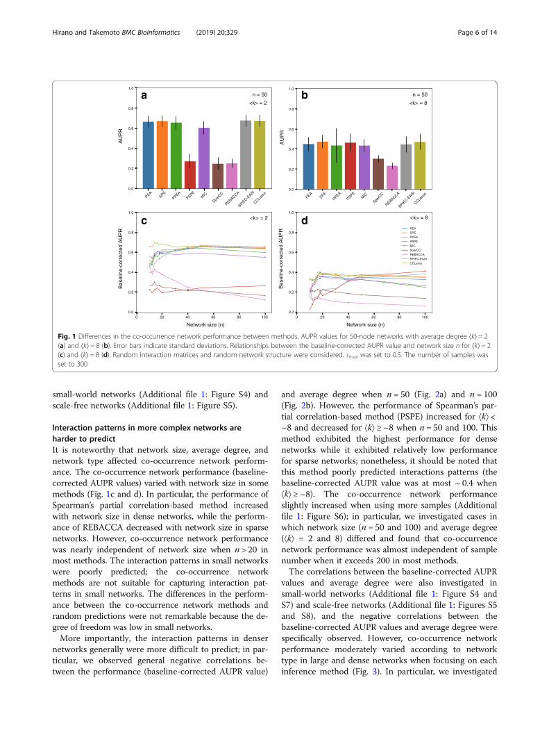
ces constructed based on random network structures(Fig. 1). We found that co-occurrence network perform-ance (AUPR value) was moderate. For example, theAUPR value was at most ~ 0.65 when network size (thenumber of species) n = 50 and average degree ⟨k⟩ = 2(Fig. 1a), and it was at most ~ 0.45 when n = 50 and

⟨k⟩ = 8 (Fig. 1b). As expected from limitations due to theconstant sum constraint, the performance of the clas-sical co-occurrence network methods (e.g., Pearson’scorrelation) generally decreased when using compos-itional data (Additional file 1: Figure S3), and the per-formance of the partial correlation-based methodsdeclined largely.More importantly, we found that the performance of

the compositional-data co-occurrence network methodswere almost equal to or less than that of classical methods,excluding Spearman’s partial correlation-based method; inparticular, the performance of some compositional-datamethods was lower than that of the classical methods.Specifically, the AUPR values of SparCC, an earliercompositional-data method, were lower than those ofPearson’s correlation [p < 2.2e–16 using t-test when n = 50and ⟨k⟩ = 2 (Fig. 1a) and p < 2.2e–16 using t-test when n =50 and ⟨k⟩ = 8 (Fig. 1b)]. Moreover, The AUPR values ofREBACCA, a later compositional-data method, were alsolower than those of Pearson’s correlation [p < 2.2e–16using t-test when n = 50 and ⟨k⟩ = 2 (Fig. 1a) and p < 2.2e–16 using t-test when n = 50 and ⟨k⟩ = 8 (Fig. 1b)]. For 50-node networks, the performance of CCLasso and SPIEC-EASI was similar to that of classical methods when ⟨k⟩ = 2(Fig. 1a) and ⟨k⟩ = 8 (Fig. 1b). However, the performance oflater compositional-data methods (e.g., CCLasso) washigher than that of the earlier compositional-data method(i.e., SparCC). Specifically, the AUPR values of CCLassowere lower than those of SparCC [p < 2.2e–16 using t-testwhen n = 50 and ⟨k⟩ = 2 (Fig. 1a) and p = 3.2e–7 using t-test when n = 50 and ⟨k⟩ = 8 (Fig. 1b)].The graphical model-based methods were not more effi-

cient than the correlation-based methods. Spearman’s partialcorrelation-based method was inferior to Pearson’s correl-ation-based method (p < 2.2e–16 using t-test) and Spear-man’s correlation-based method (p < 2.2e–16 using t-test)when n= 50 and ⟨k⟩= 2 (Fig. 1a); however, the AUPR valueof Spearman’s partial correlation-based method was similarto that of Pearson’s and Spearman’s correlation-basedmethods when n= 50 and ⟨k⟩ = 8 (Fig. 1b). Both Pearson’spartial correlation-based method and Pearson’s correlation-based method exhibited similar performance. The perform-ance of the graphical model-based method for compositionaldata (SPIEC-EASI) was similar to that of other correlation-based methods (e.g., Pearson’s correlation), although it washigher than that of the correlation-based methods for com-positional data. Specifically, the AUPR values of SPIEC-EASIwere higher than those of SparCC [p < 2.2e–16 using t-testwhen n= 50 and ⟨k⟩= 2 (Fig. 1a) and p < 2.2e–16 using t-testwhen n= 50 and ⟨k⟩= 8 (Fig. 1b)].Co-occurrence network performance was evaluated

when the average degree (Fig. 1a and b) and number ofnodes (network size; Fig. 1c and d) varied; moreover, itwas also examined for other types of network structure:

Hirano and Takemoto BMC Bioinformatics (2019) 20:329 Page 5 of 14

small-world networks (Additional file 1: Figure S4) andscale-free networks (Additional file 1: Figure S5).

Interaction patterns in more complex networks areharder to predictIt is noteworthy that network size, average degree, andnetwork type affected co-occurrence network perform-ance. The co-occurrence network performance (baseline-corrected AUPR values) varied with network size in somemethods (Fig. 1c and d). In particular, the performance ofSpearman’s partial correlation-based method increasedwith network size in dense networks, while the perform-ance of REBACCA decreased with network size in sparsenetworks. However, co-occurrence network performancewas nearly independent of network size when n > 20 inmost methods. The interaction patterns in small networkswere poorly predicted; the co-occurrence networkmethods are not suitable for capturing interaction pat-terns in small networks. The differences in the perform-ance between the co-occurrence network methods andrandom predictions were not remarkable because the de-gree of freedom was low in small networks.More importantly, the interaction patterns in denser

networks generally were more difficult to predict; in par-ticular, we observed general negative correlations be-tween the performance (baseline-corrected AUPR value)

and average degree when n = 50 (Fig. 2a) and n = 100(Fig. 2b). However, the performance of Spearman’s par-tial correlation-based method (PSPE) increased for ⟨k⟩ <~8 and decreased for ⟨k⟩ ≥ ~8 when n = 50 and 100. Thismethod exhibited the highest performance for densenetworks while it exhibited relatively low performancefor sparse networks; nonetheless, it should be noted thatthis method poorly predicted interactions patterns (thebaseline-corrected AUPR value was at most ~ 0.4 when⟨k⟩ ≥ ~8). The co-occurrence network performanceslightly increased when using more samples (Additionalfile 1: Figure S6); in particular, we investigated cases inwhich network size (n = 50 and 100) and average degree(⟨k⟩ = 2 and 8) differed and found that co-occurrencenetwork performance was almost independent of samplenumber when it exceeds 200 in most methods.The correlations between the baseline-corrected AUPR

values and average degree were also investigated insmall-world networks (Additional file 1: Figure S4 andS7) and scale-free networks (Additional file 1: Figures S5and S8), and the negative correlations between thebaseline-corrected AUPR values and average degree werespecifically observed. However, co-occurrence networkperformance moderately varied according to networktype in large and dense networks when focusing on eachinference method (Fig. 3). In particular, we investigated

PEASPE

PPEAPSPE

MIC

SparC

C

REBACCA

SPIEC-E

ASI

CCLass

o0.0

0.2

0.4

0.6

0.8

1.0

PEASPE

PPEAPSPE

MIC

SparC

C

REBACCA

SPIEC-E

ASI

CCLass

o0.0

0.2

0.4

0.6

0.8

1.0

0 20 40 60 80 1000.0

0.2

0.4

0.6

0.8

1.0

RP

UA

RP

UA detcerroc-enilesa

B

AU

PR

Bas

elin

e-co

rrec

ted

AU

PR

0 20 40 60 80 100

Network size (n)Network size (n)

0.0

0.2

0.4

0.6

0.8

1.0

n = 50

<k> = 2

n = 50

<k> = 8

<k> = 2 <k> = 8

a

c

b

dPEASPEPPEAPSPEMICSparCCREBACCASPIEC-EASICCLasso

Fig. 1 Differences in the co-occurrence network performance between methods. AUPR values for 50-node networks with average degree ⟨k⟩ = 2(a) and ⟨k⟩ = 8 (b). Error bars indicate standard deviations. Relationships between the baseline-corrected AUPR value and network size n for ⟨k⟩ = 2(c) and ⟨k⟩ = 8 (d). Random interaction matrices and random network structure were considered. smax was set to 0.5. The number of samples wasset to 300

Hirano and Takemoto BMC Bioinformatics (2019) 20:329 Page 6 of 14

Pearson’s correlation-based method (a classical correl-ation-based method; Fig. 3a and b), Pearson’s partial cor-relation-based method (a classical graphical model-basedmethod; Fig. 3c and d), CCLasso (a correlation-basedmethod for compositional data; Fig. 3e and f), andSPEIC-EASI (a graphical model-based method for com-positional data; Fig. 3g and h). In general, the lowest per-formance was observed for scale-free networks, whilethe highest performance was observed for small-worldnetworks (Fig. 3). Specifically, the baseline-corrected AUPRvalues for scale-free networks were lower than those forsmall world networks when n= 100 and ⟨k⟩= 8 (p < 2.2e–16using t-test for Pearson’s correlation-based method; p=7.7e–5 using t-test for Pearson’s partial correlation-based

method; p= 0.027 using t-test for CCLasso; p= 1.9e–13using t-test for SPEIC-EASI). Moreover, the baseline-corrected AUPR values for scale-free networks were lowerthan those for random networks when n= 100 and ⟨k⟩= 8for Pearson’s correlation-based method (p= 2.9e–3 using t-test) and SPEIC-EASI (p= 7.4e–3 using t-test).The results indicating that compositional-data co-

occurrence network methods were not more efficientthan classical methods and that interaction patterns inmore complex networks are more difficult to predict(Figs. 1, 2 and 3) were also generally confirmed in theother types of interactions matrices: competitive (Add-itional file 1: Figures S9–S11), mutualistic (Additionalfile 1: Figures S12 and S13), predator–prey (Additional

0.0 2.5 5.0 7.5 10.0 12.5 15.0 17.5 20.00.0

0.2

0.4

0.6

0.8

1.0

0.0 2.5 5.0 7.5 10.0 12.5 15.0 17.5 20.00.0

0.2

0.4

0.6

0.8

1.0

Bas

elin

e-co

rrec

ted

AU

PR

Bas

elin

e-co

rrec

ted

AU

PR

>k< eerged egarevA>k< eerged egarevA

001 = n05 = n baPEASPEPPEAPSPEMICSparCCREBACCASPIEC-EASICCLasso

(r = –0.92, p < 2.2e–16)s

(r = –0.92, p < 2.2e–16)s

(r = –0.79, p < 2.2e–16)s

(r = –0.93, p < 2.2e–16)s

(r = –0.65, p < 2.2e–16)(r = –0.65, p < 2.2e–16)s

(r = –0.86, p < 2.2e–16)s

(r = –0.93, p < 2.2e–16)s

(r = –0.87, p < 2.2e–16)s

(r = 0.28, p = 1.1e–6)s

PEASPEPPEAPSPEMICSparCCREBACCASPIEC-EASICCLasso

(r = –0.93, p < 2.2e–16)s

(r = –0.92, p < 2.2e–16)s

(r = –0.87, p < 2.2e–16)s

(r = –0.92, p < 2.2e–16)s

(r = –0.65, p < 2.2e–16)(r = –0.56, p < 2.2e–16)s

(r = –0.85, p < 2.2e–16)s

(r = –0.93, p < 2.2e–16)s

(r = –0.86, p < 2.2e–16)s

(r = 0.20, p = 1.1e–3)s

Fig. 2 Relationships between co-occurrence network performance (baseline-corrected AUPR value) and average degree when network size n = 50(a) and n = 100 (b). Random interaction matrices and random network structure were considered. smax was set to 0.5. The number of sampleswas set to 300. The baseline-corrected AUPR values of CCLasso were not calculated when ⟨k⟩ > 10 in 100-node networks because of highcomputational costs. rs and p indicate the Spearman’s rank correlation coefficient and the associated p-value. The raw values (i.e., the valuesbefore averaging) were used for calculating rs

a

b

c

d

e

f

g

h

Fig. 3 Relationships between co-occurrence network performance (AUPR value) and network size n according to the network types: randomnetworks (random), scale-free networks (sf), and small-world networks (sw). Random interaction matrices were considered. The cases of sparsenetworks (⟨k⟩ = 2; top panels) and dense networks (⟨k⟩ = 8; bottom panels) are shown. As representative examples, Pearson’s correlation-basedmethod (a classical correlation-based method; a and b), Pearson’s partial correlation-based method (a classical graphical model-based method; cand d), CCLasso (a correlation-based method for compositional data; e and f), and SPEIC-EASI (a graphical model-based method forcompositional data; g and h) are shown. smax was set to 0.5. The number of samples was set to 300

Hirano and Takemoto BMC Bioinformatics (2019) 20:329 Page 7 of 14

file 1: Figures S14–S16), and mutualism-competitionmixture interaction matrices (Additional file 1: FiguresS17–S19).

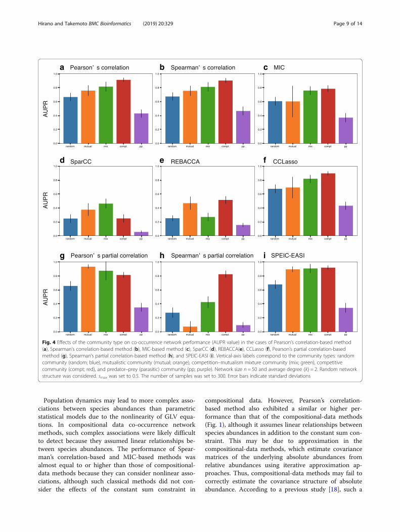
Predator-prey (parasitic) interactions decrease co-occurrence network performanceThe types of interaction matrices notably affected co-occurrence network performance (Fig. 4). Specifically, inmost methods, the interaction patterns in predator–prey(parasitic) communities (interaction matrices) were themost difficult to predict, while those in competitivecommunities were the easiest to predict. Specifically, theAUPR values for predator–prey communities were sig-nificantly lower than those for competitive communitiesfor Pearson’s correlation-based method (p < 2.2e–16using t-test; Fig. 4a), Spearman’s correlation-basedmethod (p < 2.2e–16 using t-test; Fig. 4b), MIC-basedmethod (p < 2.2e–16 using t-test; Fig. 4c), SparCC (p <2.2e–16 using t-test; Fig. 4d), REBACCA (p < 2.2e–16using t-test; Fig. 4e), CCLasso (p < 2.2e–16 using t-test;Fig. 4f ), Pearson’s partial correlation-based method (p <2.2e–16 using t-test; Fig. 4g), Spearman’s partialcorrelation-based method (p < 2.2e–16 using t-test; Fig.4h), and SPEIC-EASI (p < 2.2e–16 using t-test; Fig. 4i).Additionally, co-occurrence network methods relativelyaccurately predicted interactions patterns in mutualcommunities and competition–mutualism mixture com-munities; however, they described the interaction pat-terns in random communities poorly. Specifically, theAUPR values for random communities also were signifi-cantly lower than those for competitive communities forPearson’s correlation-based method (p < 2.2e–16 using t-test; Fig. 4a), Spearman’s correlation-based method (p <2.2e–16 using t-test; Fig. 4b), MIC-based method (p <2.2e–16 using t-test; Fig. 4c), REBACCA (p < 2.2e–16using t-test; Fig. 4e), CCLasso (p < 2.2e–16 using t-test;Fig. 4f ), Pearson’s partial correlation-based method (p <2.2e–16 using t-test; Fig. 4g), Spearman’s partialcorrelation-based method (p < 2.2e–16 using t-test; Fig.4h), and SPEIC-EASI (p < 2.2e–16 using t-test; Fig. 4i).Similar tendencies of the effect of interaction types onco-occurrence network performance were observed invarying network sizes (i.e., n = 20 and 100; Additional file1: Figure S20), average degrees (i.e., ⟨k⟩ = 4 and 8; Add-itional file 1: Figure S21), and network structures (i.e.,small-world and scale-free network structures; Add-itional file 1: Figure S22).We hypothesized that co-occurrence network per-

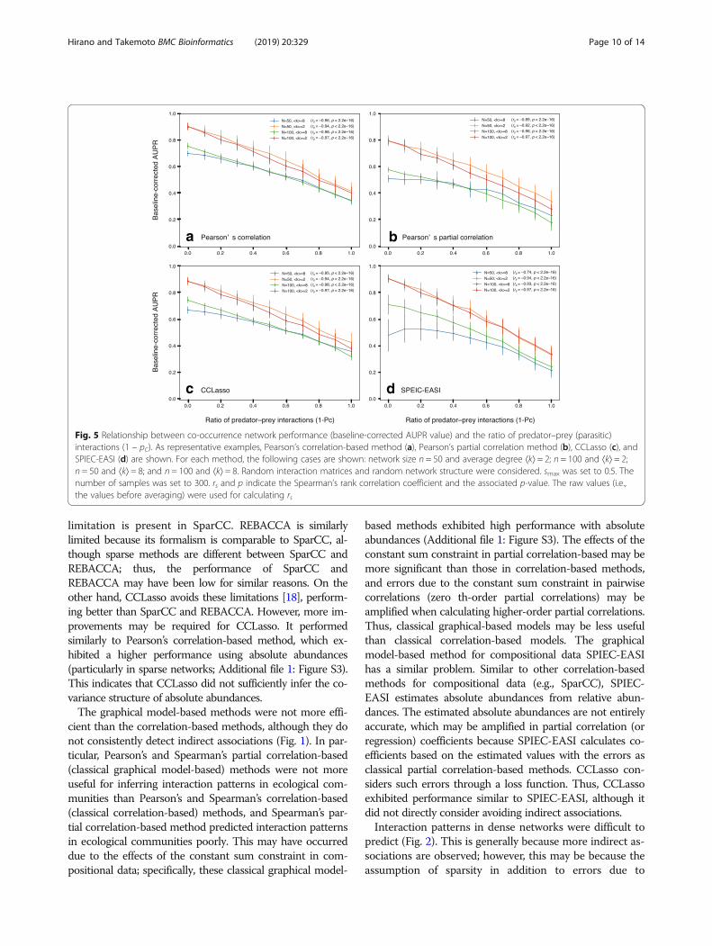
formance decreases as the ratio of predator–prey (para-sitic) interactions increases because the worstperformance and second worst performance were ob-served for predator–prey and random communities, re-spectively. Note that almost half of the interactions arespontaneously set to predator–prey interactions in

random communities (see “Generation of relative abun-dance data using a dynamical model” section). To testthis hypothesis, we considered interaction matrices con-sisting of a mixture of competitive and predator–preyinteractions because co-occurrence network perform-ance was best and worst in competitive and predator–prey (parasitic) communities, respectively. In particular,we considered competition–parasitism mixture commu-nities with the ratio pC of competitive interactions to allinteractions and investigated the relationship betweenthe ratio of predator–prey interactions (i.e., 1 − pC) andAUPR values. As representative examples, we investigatedPearson’s correlation-based method (a classical correlation-based method; Fig. 5a), Pearson’s partial correlation method(a classical graphical model-based method; Fig. 5b), CCLasso(a correlation-based method for compositional data; Fig. 5c),and SPIEC-EASI (a graphical model-based for compositionaldata; Fig. 5d). As expected, we found negative correlationsbetween co-occurrence network performance (AUPR value)and the ratio of predator–prey interactions (Fig. 5). Suchnegative correlations were also observed in cases with differ-ent network sizes (n= 50 and 100) and average degrees(⟨k⟩= 2 and 8).

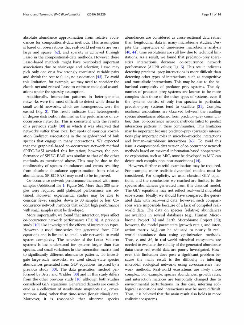
DiscussionInspired by previous studies [30], we evaluated how wellco-occurrence network methods recapitulate microbialecological networks using a population dynamics model;co-occurrence network methods are often used for dis-cussing species interactions although they only infer eco-logical associations. We compared wide-rangingmethods using realistic simulations. Our results provideadditional and complementary insights into co-occurrence network approaches in microbiome studies.The results indicate that compositional-data methods,

such as SparCC and SPIEC-EASI, are less useful in infer-ring microbial ecological networks than previouslythought. As shown in Fig. 1, the performance (AUPRvalues) of the compositional-data methods was moder-ate; furthermore, these compositional-data methodswere not more efficient than the classical methods, suchas Pearson’s correlation-based method. This result is in-consistent with previous studies [17, 18, 20]. This dis-crepancy was mainly due to differences in co-occurrencenetwork method validation between this and previousstudies. Specifically, previous studies generated abun-dance data from a multivariable distribution with a givenmean and covariance matrix and examined how accur-ately co-occurrence network methods describe the ori-ginal covariance matrix structure. However, this studyconsidered species abundances determined throughpopulation dynamics (GLV equations) and examinedhow accurately the methods reproduced interaction pat-terns in ecological communities [30].

Hirano and Takemoto BMC Bioinformatics (2019) 20:329 Page 8 of 14

Population dynamics may lead to more complex asso-ciations between species abundances than parametricstatistical models due to the nonlinearity of GLV equa-tions. In compositional data co-occurrence networkmethods, such complex associations were likely difficultto detect because they assumed linear relationships be-tween species abundances. The performance of Spear-man’s correlation-based and MIC-based methods wasalmost equal to or higher than those of compositional-data methods because they can consider nonlinear asso-ciations, although such classical methods did not con-sider the effects of the constant sum constraint in

compositional data. However, Pearson’s correlation-based method also exhibited a similar or higher per-formance than that of the compositional-data methods(Fig. 1), although it assumes linear relationships betweenspecies abundances in addition to the constant sum con-straint. This may be due to approximation in thecompositional-data methods, which estimate covariancematrices of the underlying absolute abundances fromrelative abundances using iterative approximation ap-proaches. Thus, compositional-data methods may fail tocorrectly estimate the covariance structure of absoluteabundance. According to a previous study [18], such a

a b c

d e f

g h i

Fig. 4 Effects of the community type on co-occurrence network performance (AUPR value) in the cases of Pearson’s correlation-based method(a), Spearman’s correlation-based method (b), MIC-based method (c), SparCC (d), REBACCA(e), CCLasso (f), Pearson’s partial correlation-basedmethod (g), Spearman’s partial correlation-based method (h), and SPEIC-EASI (i). Vertical-axis labels correspond to the community types: randomcommunity (random; blue), mutualistic community (mutual; orange), competition–mutualism mixture community (mix; green), competitivecommunity (compt; red), and predator–prey (parasitic) community (pp; purple). Network size n = 50 and average degree ⟨k⟩ = 2. Random networkstructure was considered. smax was set to 0.5. The number of samples was set to 300. Error bars indicate standard deviations

Hirano and Takemoto BMC Bioinformatics (2019) 20:329 Page 9 of 14

limitation is present in SparCC. REBACCA is similarlylimited because its formalism is comparable to SparCC, al-though sparse methods are different between SparCC andREBACCA; thus, the performance of SparCC andREBACCA may have been low for similar reasons. On theother hand, CCLasso avoids these limitations [18], perform-ing better than SparCC and REBACCA. However, more im-provements may be required for CCLasso. It performedsimilarly to Pearson’s correlation-based method, which ex-hibited a higher performance using absolute abundances(particularly in sparse networks; Additional file 1: Figure S3).This indicates that CCLasso did not sufficiently infer the co-variance structure of absolute abundances.The graphical model-based methods were not more effi-

cient than the correlation-based methods, although they donot consistently detect indirect associations (Fig. 1). In par-ticular, Pearson’s and Spearman’s partial correlation-based(classical graphical model-based) methods were not moreuseful for inferring interaction patterns in ecological com-munities than Pearson’s and Spearman’s correlation-based(classical correlation-based) methods, and Spearman’s par-tial correlation-based method predicted interaction patternsin ecological communities poorly. This may have occurreddue to the effects of the constant sum constraint in com-positional data; specifically, these classical graphical model-

based methods exhibited high performance with absoluteabundances (Additional file 1: Figure S3). The effects of theconstant sum constraint in partial correlation-based may bemore significant than those in correlation-based methods,and errors due to the constant sum constraint in pairwisecorrelations (zero th-order partial correlations) may beamplified when calculating higher-order partial correlations.Thus, classical graphical-based models may be less usefulthan classical correlation-based models. The graphicalmodel-based method for compositional data SPIEC-EASIhas a similar problem. Similar to other correlation-basedmethods for compositional data (e.g., SparCC), SPIEC-EASI estimates absolute abundances from relative abun-dances. The estimated absolute abundances are not entirelyaccurate, which may be amplified in partial correlation (orregression) coefficients because SPIEC-EASI calculates co-efficients based on the estimated values with the errors asclassical partial correlation-based methods. CCLasso con-siders such errors through a loss function. Thus, CCLassoexhibited performance similar to SPIEC-EASI, although itdid not directly consider avoiding indirect associations.Interaction patterns in dense networks were difficult to

predict (Fig. 2). This is generally because more indirect as-sociations are observed; however, this may be because theassumption of sparsity in addition to errors due to

a b

c d

Fig. 5 Relationship between co-occurrence network performance (baseline-corrected AUPR value) and the ratio of predator–prey (parasitic)interactions (1 – pC). As representative examples, Pearson’s correlation-based method (a), Pearson’s partial correlation method (b), CCLasso (c), andSPIEC-EASI (d) are shown. For each method, the following cases are shown: network size n = 50 and average degree ⟨k⟩ = 2; n = 100 and ⟨k⟩ = 2;n = 50 and ⟨k⟩ = 8; and n = 100 and ⟨k⟩ = 8. Random interaction matrices and random network structure were considered. smax was set to 0.5. Thenumber of samples was set to 300. rs and p indicate the Spearman’s rank correlation coefficient and the associated p-value. The raw values (i.e.,the values before averaging) were used for calculating rs

Hirano and Takemoto BMC Bioinformatics (2019) 20:329 Page 10 of 14

absolute abundance approximation from relative abun-dances for compositional-data methods. This assumptionis based on observations that real-world networks are verylarge and sparse [42], and sparsity is achieved throughLasso in the compositional-data methods. However, theseLasso-based methods might have overlooked importantassociations due to shrinkage and selection; Lasso maypick only one or a few strongly correlated variable pairsand shrink the rest to 0, i.e., no association [43]. To avoidthis limitation, for example, we may need to consider theelastic-net and relaxed Lasso to estimate ecological associ-ations under the sparsity assumption.Additionally, interaction patterns in heterogeneous

networks were the most difficult to detect while those insmall-world networks, which are homogenous, were theeasiest (Fig. 3). This result indicates that heterogeneityin degree distribution diminishes the performance of co-occurrence networks. This is consistent with the resultsof a previous study [30] in which it was observed thatnetworks suffer from local hot spots of spurious correl-ation (indirect association) in the neighborhood of hubspecies that engage in many interactions. We expectedthat the graphical-based co-occurrence network methodSPIEC-EASI avoided this limitation; however, the per-formance of SPIEC-EASI was similar to that of the othermethods, as mentioned above. This may be due to thenonlinearity of species abundances and errors resultingfrom absolute abundance approximation from relativeabundances. SPIEC-EASI may need to be improved.Co-occurrence network performance increased with more

samples (Additional file 1: Figure S6). More than 200 sam-ples were required until plateaued performance was ob-tained. However, experimental studies may be able toconsider fewer samples, down to 30 samples or less. Co-occurrence network methods that exhibit high performancewith small samples must be developed.More importantly, we found that interaction types affect

co-occurrence network performance (Fig. 4). A previousstudy [10] also investigated the effects of interaction types.However, it used time-series data generated from GLVequations and is limited to small-scale networks to avoidsystem complexity. The behavior of the Lotka–Volterrasystems is less understood for systems larger than twospecies, and small variations in the interaction matrix leadto significantly different abundance patterns. To investi-gate large-scale networks, we used steady-state speciesabundances generated from GLV equations, inspired by aprevious study [30]. The data generation method per-formed by Berry and Widder [30] and in this study differsfrom the other previous study [10] although both studiesconsidered GLV equations. Generated datasets are consid-ered as a collection of steady-state snapshots (i.e., cross-sectional data) rather than time-series (longitudinal) data.Moreover, it is reasonable that observed species

abundances are considered as cross-sectional data ratherthan longitudinal data in many microbiome studies. Des-pite the importance of time-series microbiome analysis[40, 44], time resolutions are still low due to technical lim-itations. As a result, we found that predator–prey (para-sitic) interactions decrease co-occurrence networkperformance (AUPR values; Fig. 5). This result indicatesdetecting predator–prey interactions is more difficult thandetecting other types of interactions, such as competitiveand mutualistic interactions. This may be due to the be-havioral complexity of predator–prey systems. The dy-namics of predator–prey systems are known to be morecomplex than those of the other types of systems, even ifthe systems consist of only two species; in particular,predator–prey systems tend to oscillate [31]. Complexnonlinear associations are observed between the resultingspecies abundances obtained from predator–prey communi-ties; thus, co-occurrence network methods failed to predictinteraction patterns in these communities. This limitationmay be important because predator–prey (parasitic) interac-tions play important roles in microbe–microbe interactionsand human–microbiome interactions [45]. To avoid thisissue, a compositional-data version of co-occurrence networkmethods based on maximal information-based nonparamet-ric exploration, such as MIC, must be developed as MIC candetect such complex nonlinear associations [14].However, further careful examination may be required.

For example, more realistic dynamical models must beconsidered. For simplicity, we used classical GLV equa-tions, and the conclusions we reached are limited to thespecies abundances generated from this classical model.The GLV equations may not reflect real-world microbialecosystems. Ideally, we should have compared the gener-ated data with real-world data; however, such compari-sons were impossible because of a lack of compiled real-world data. The data on species (relative) abundancesare available in several databases (e.g., Human Micro-biome Project [4] and Earth Microbiome Project [5]);however, the model parameters (growth rate ri and inter-action matrix Mij) can be adjusted to nearly fit real-world abundance data using optimization methods.Thus, ri and Mij in real-world microbial ecosystems areneeded to evaluate the validity of the generated abundancedata; these real-world data are poorly investigated. How-ever, this limitation does pose a significant problem be-cause the main result is the difficulty in inferringmicrobial ecological networks using co-occurrence net-work methods. Real-world ecosystems are likely morecomplex. For example, species abundances, growth rates,and interaction matrices are temporally changed due toenvironmental perturbations. In this case, inferring eco-logical associations and interactions may be more difficult.Thus, it is believed that the main result also holds in morerealistic ecosystems.

Hirano and Takemoto BMC Bioinformatics (2019) 20:329 Page 11 of 14

To more accurately detect ecological associationsand directly detect species–species interactions, how-ever, alternative methods are also needed. For ex-ample, a method grounded in maximum entropymodels of statistical physics has been proposed to dif-ferentiate direct and indirect associations [46]. Thedifficulty of interpreting species–species interactionsfrom co-occurrence data has been pointed out incommunity ecology [47]. To overcome this difficulty,Markov networks (Markov random fields) have been usedfor inferring species–species interactions from co-occurrencedata in community ecology [48]. Dynamics (time series)-based methods are also useful. For example, convergentcross mapping [49] may be useful. This method is based onnonlinear state-space reconstruction and can distinguishcausality in complex systems from correlation. The sparse S-map method [50] is a data-oriented equation-free modelingapproach for multispecies ecological dynamics whose inter-action topology is unknown, and it generates a sparse inter-action network from a multivariate ecological time serieswithout presuming any mathematical formulation for theunderlying microbial processes. Another method, proposedby Xiao et al. [51], is based on Jacobian (community) matri-ces and can infer network topology and inter-taxa interactiontypes without assuming any particular population dynamicsmodel from steady-state abundance data. Randomly distrib-uted embedding [52] is a model-free framework thatachieves accurate future-state prediction based on short-term high-dimensional data. However, these methods arenot applicable to compositional data and must be improved.Thus, we did not consider these methods in this study.

ConclusionsOur findings indicate that co-occurrence networkmethods are not efficient in interpreting interspe-cies interactions in microbiome studies becausethese methods only infer ecological associations.However, these results do not diminish the import-ance of co-occurrence network approaches. Co-occurrence network approaches remain a challen-ging research topic in the post-genomic era due tothe importance of human [4] and ecological micro-biomes [5]. Our findings highlight the need for fur-ther careful investigation of the validity of thesewidely used methods and development of moresuitable approaches for inferring microbial eco-logical networks.

Additional files

Additional file 1: Supplementary figures. (PDF 3162 kb)

Additional file 2: R source codes for generating datasets and forevaluating co-occurrence network performance. (ZIP 5 kb)

AbbreviationsAUPR: area under the precision–recall curve; CCLasso: correlation inferencefor compositional data through Lasso; GLV: generalized Lotka–Volterra;Lasso: least absolute shrinkage and selection operator; MIC: maximalinformation coefficient; PEA: Pearson’s correlation; PPEA: Pearson’s partialcorrelation; PR: precision–recall; PSPE: Spearman’s partial correlation;REBACCA: regularized estimation of the basis covariance based oncompositional data; SparCC: sparse correlations for compositional data;SPE: Spearman’s correlation; SPIEC-EASI: sparse inverse covariance estimationfor ecological association inference

AcknowledgmentsWe would like to thank Editage (www.editage.jp) for English languageediting.

Authors’ contributionsHH and KT conceived and designed the study. HH and KT prepared thesource codes for numerical simulations. HH performed numerical simulations.HH and KT interpreted the results. HH and KT drafted the manuscript. Allauthors read and approved the final manuscript.

FundingThis study was supported by JSPS KAKENHI Grant Number JP17H04703. Thefunding body had no role in the design, collection, analysis, or interpretationof this study.

Availability of data and materialsAll data generated and analyzed during this study are included in thispublished article and its supplementary information files.

Ethics approval and consent to participateNot applicable.

Consent for publicationNot applicable.

Competing interestsThe authors declare that they have no competing interests.

Received: 15 March 2019 Accepted: 27 May 2019

References1. Faust K, Sathirapongsasuti JF, Izard J, Segata N, Gevers D, Raes J, et al.

Microbial co-occurrence relationships in the human microbiome. OuzounisCA, editor. PLoS Comput Biol [Internet] 2012;8:e1002606. Available from:http://dx.plos.org/10.1371/journal.pcbi.1002606

2. Butler S, O’Dwyer JP. Stability criteria for complex microbial communities.Nat Commun [Internet] Springer US; 2018;9:2970. Available from: http://www.nature.com/articles/s41467-018-05308-z

3. Coyte KZ, Schluter J, Foster KR. The ecology of the microbiome: networks,competition, and stability. Science [Internet]. 2015;350:663–6. Available from:http://www.sciencemag.org/cgi/doi/10.1126/science.aad2602

4. Cho I, Blaser MJ. The human microbiome: at the interface of health anddisease. Nat Rev Genet [Internet]. 2012;13:260–70. Available from: http://www.nature.com/doifinder/10.1038/nrg3182

5. Gilbert JA, Jansson JK, Knight R. The earth microbiome project: successesand aspirations. BMC Biol [Internet] 2014;12:69. Available from: http://bmcbiol.biomedcentral.com/articles/10.1186/s12915-014-0069-1

6. Quince C, Walker AW, Simpson JT, Loman NJ, Segata N. Shotgunmetagenomics, from sampling to analysis. Nat Biotechnol [Internet]. 2017;35:833–44. Available from: http://www.nature.com/doifinder/10.1038/nbt.3935

7. Gentile CL, Weir TL. The gut microbiota at the intersection of diet andhuman health. Science [Internet]. 2018;362:776–80. Available from:http://science.sciencemag.org/cgi/content/short/362/6416/776

8. Duvallet C, Gibbons SM, Gurry T, Irizarry RA, Alm EJ. Meta-analysis of gutmicrobiome studies identifies disease-specific and shared responses. NatCommun [Internet]. 2017;8:1784. Available from: https://www.nature.com/articles/s41467-017-01973-8.pdf

9. Delgado-Baquerizo M, Oliverio AM, Brewer TE, Benavent-González A,Eldridge DJ, Bardgett RD, et al. A global atlas of the dominant bacteria

Hirano and Takemoto BMC Bioinformatics (2019) 20:329 Page 12 of 14

found in soil. Science [Internet]. 2018;359:320–5. Available from: http://www.sciencemag.org/lookup/doi/10.1126/science.aap9516

10. Weiss S, Van Treuren W, Lozupone C, Faust K, Friedman J, Deng Y, et al.Correlation detection strategies in microbial data sets vary widely insensitivity and precision. ISME J. [Internet]. Nat Publ Group; 2016;10:1669–81.Available from: https://doi.org/10.1038/ismej.2015.235

11. Langfelder P, Horvath S. WGCNA: an R package for weighted correlation networkanalysis. BMC Bioinformatics [Internet] 2008;9: 559. Available from: https://bmcbioinformatics.biomedcentral.com/articles/10.1186/1471-2105-9-559

12. Zhou J, Deng Y, Luo F, He Z, Tu Q, Zhi X. Functional molecular ecologicalnetworks. MBio [Internet]. 2010 [cited 2013 May 29];1. Available from: http://www.pubmedcentral.nih.gov/articlerender.fcgi?artid=2953006&tool=pmcentrez&rendertype=abstract

13. Obayashi T, Aoki Y, Tadaka S, Kagaya Y, Kinoshita K. ATTED-II in 2018: a plantCoexpression database based on investigation of the statistical property ofthe mutual rank index. Plant Cell Physiol [Internet]. 2018;59:e3–e3. Availablefrom: https://academic.oup.com/pcp/article/59/1/e3/4690683

14. Reshef DN, Reshef YA, Finucane HK, Grossman SR, Mc Vean G, Turnbaugh PJ, etal. Detecting novel associations in large data sets. Science [Internet]. 2011 [cited2013 Feb 27]; 334:1518–24. Available from: http://www.pubmedcentral.nih.gov/articlerender.fcgi?artid=3325791&tool=pmcentrez&rendertype=abstract

15. Aitchison J. A new approach to null correlations of proportions. J Int AssocMath Geol [Internet] 1981;13:175–89. Available from: http://link.springer.com/10.1007/BF01031393

16. Friedman J, Alm EJ. Inferring Correlation Networks from Genomic Survey Data.von Mering C, editor. PLoS Comput. Biol. [Internet]. 2012 [cited 2012 Sep 21];8:e1002687. Available from: http://dx.plos.org/10.1371/journal.pcbi.1002687

17. Ban Y, An L, Jiang H. Investigating microbial co-occurrence patterns basedon metagenomic compositional data. Bioinformatics. 2015;31:3322–9.

18. Fang H, Huang C, Zhao H, Deng M. CCLasso: correlation inference forcompositional data through lasso. Bioinformatics. 2015;31:3172–80.

19. Johansson Å, Løset M, Mundal SB, Johnson MP, Freed KA, Fenstad MH, et al.Partial correlation network analyses to detect altered gene interactions inhuman disease: using preeclampsia as a model. Hum Genet [Internet] 2011;129:25–34. Available from: http://link.springer.com/10.1007/s00439-010-0893-5

20. Kurtz ZD, Mueller CL, Miraldi ER, Littman DR, Blaser MJ, Bonneau RA, et al.Sparse and compositionally robust inference of microbial ecologicalnetworks. von Mering C, editor. PLOS Comput. Biol. [Internet]. 2014;11:e1004226. Available from: http://dx.plos.org/10.1371/journal.pcbi.1004226

21. Ramanan D, Bowcutt R, Lee SC, Tang MS, Kurtz ZD, Ding Y, et al. Helminthinfection promotes colonization resistance via type 2 immunity. Science[Internet]. 2016;352:608–12. Available from: http://www.sciencemag.org/lookup/doi/10.1126/science.aaf3229

22. Coelho LP, Kultima JR, Costea PI, Fournier C, Pan Y, Czarnecki-Maulden G, et al.Similarity of the dog and human gut microbiomes in gene content andresponse to diet. Microbiome [Internet]. 2018;6:72. Available from: https://microbiomejournal.biomedcentral.com/articles/10.1186/s40168-018-0450-3.

23. Flemer B, Warren RD, Barrett MP, Cisek K, Das A, Jeffery IB, et al. The oral microbiotain colorectal cancer is distinctive and predictive. Gut [Internet]. 2018;67:1454–63.Available from: http://gut.bmj.com/lookup/doi/10.1136/gutjnl-2017-314814

24. Burns MB, Montassier E, Abrahante J, Priya S, Niccum DE, Khoruts A, et al. Colorectalcancer mutational profiles correlate with defined microbial communities in thetumor microenvironment. Fearon ER, editor. PLOS Genet [Internet] 2018;14:e1007376. Available from: https://dx.plos.org/10.1371/journal.pgen.1007376

25. Toju H, Yamamoto S, Tanabe AS, Hayakawa T, Ishii HS. Network modules and hubsin plant-root fungal biomes. J R Soc Interface [Internet]. 2016;13:20151097. Availablefrom: http://rsif.royalsocietypublishing.org/lookup/doi/10.1098/rsif.2015.1097

26. Shen C, Shi Y, Fan K, He J-S, Adams JM, Ge Y, et al. Soil pH dominateselevational diversity pattern for bacteria in high elevation alkaline soils on theTibetan plateau. FEMS Microbiol Ecol [Internet]. 2019;95. Available from: https://academic.oup.com/femsec/article/doi/10.1093/femsec/fiz003/5281419

27. Goss-Souza D, Mendes LW, Borges CD, Baretta D, Tsai SM, Rodrigues JLM. Soilmicrobial community dynamics and assembly under long-term land usechange. FEMS Microbiol Ecol [Internet]. 2017;93. Available from: https://academic.oup.com/femsec/article/doi/10.1093/femsec/fix109/4102335

28. Layeghifard M, Hwang DM, Guttman DS. Disentangling interactions in themicrobiome: a network perspective. Trends Microbiol. [internet]. Elsevier Ltd;2017;25:217–28. Available from: https://doi.org/10.1016/j.tim.2016.11.008

29. Faust K, Raes J. Microbial interactions: from networks to models. Nat RevMicrobiol [Internet]. 2012;10:538–50. Available from: http://www.nature.com/articles/nrmicro2832

30. Berry D, Widder S. Deciphering microbial interactions and detectingkeystone species with co-occurrence networks. Front Microbiol[Internet] 2014 [cited 2014 Jul 9];5:219. Available from: http://www.pubmedcentral.nih.gov/articlerender.fcgi?artid=4033041&tool=pmcentrez&rendertype=abstract

31. Allesina S, Tang S. Stability criteria for complex ecosystems. Nature[Internet]. Nature Publishing Group; 2012 [cited 2014 Jan 20];483:205–8.Available from: http://www.ncbi.nlm.nih.gov/pubmed/22343894

32. Takemoto K, Oosawa C. Introduction to complex networks: measures,statistical properties, and models. Stat Mach Learn Approaches NetwAnal. 2012:45–75.

33. Takemoto K, Iida M. Ecological networks. Encycl. Bioinforma. Comput. Biol.[internet]. Elsevier; 2019. p. 1131–41. Available from: https://linkinghub.elsevier.com/retrieve/pii/B9780128096338202033

34. Takemoto K, Kajihara K. Human impacts and climate change influencenestedness and modularity in food-web and mutualistic networks. PLoSOne [Internet]. 2016;11:e0157929. Available from: http://dx.plos.org/10.1371/journal.pone.0157929

35. Watts DJ, Strogatz SH. Collective dynamics of “small-world” networks.Nature [Internet]. 1998;393:440–2. Available from: http://www.ncbi.nlm.nih.gov/pubmed/9623998

36. Chung F, Lu L. Connected components in random graphs with givenexpected degree sequences. Ann Comb. 2002:125–45.

37. Cho YS, Kim JS, Park J, Kahng B, Kim D. Percolation transitions in scale-freenetworks under the achlioptas process. Phys. Rev. Lett. [Internet]. 2009[cited 2011 Nov 17];103:135702. Available from: http://link.aps.org/doi/10.1103/PhysRevLett.103.135702

38. Albert R, Barabási A-L. Statistical mechanics of complex networks. Rev ModPhys [Internet]. 2002 [cited 2012 Mar 7];74:47–97. Available from: http://link.aps.org/doi/10.1103/RevModPhys.74.47

39. Venturelli OS, Carr AC, Fisher G, Hsu RH, Lau R, Bowen BP, et al. Decipheringmicrobial interactions in synthetic human gut microbiome communities.Mol Syst Biol [Internet]. 2018;14:e8157. Available from: http://msb.embopress.org/lookup/doi/10.15252/msb.20178157

40. Faust K, Bauchinger F, Laroche B, de Buyl S, Lahti L, Washburne AD, et al.Signatures of ecological processes in microbial community time series.Microbiome [Internet] 2018;6:120. Available from: https://microbiomejournal.biomedcentral.com/articles/10.1186/s40168-018-0496-2

41. Mougi A, Kondoh M. Diversity of interaction types and ecologicalcommunity stability. Science [Internet]. 2012 [cited 2013 Nov 7];337:349–51. Available from: http://www.ncbi.nlm.nih.gov/pubmed/22822151

42. Cimini G, Squartini T, Saracco F, Garlaschelli D, Gabrielli A, Caldarelli G. Thestatistical physics of real-world networks. Nat. Rev. Phys. [internet]. SpringerUS; 2018;1. Available from: http://arxiv.org/abs/1810.05095%0A, https://doi.org/10.1038/s42254-018-0002-6

43. Wang S, Nan B, Rosset S, Zhu J. Random lasso. Ann Appl Stat [Internet].2011;5:468–85. Available from: http://projecteuclid.org/euclid.aoas/1300715199

44. Faust K, Lahti L, Gonze D, de Vos WM, Raes J. Metagenomics meetstime series analysis: unraveling microbial community dynamics. Curr.Opin. Microbiol. [internet]. Elsevier Ltd; 2015;25:56–66. Available from:https://doi.org/10.1016/j.mib.2015.04.004

45. Feichtmayer J, Deng L, Griebler C. Antagonistic microbial interactions:contributions and potential applications for controlling pathogens in theaquatic systems. Front Microbiol [Internet]. 2017;8:2192. Available from:http://journal.frontiersin.org/article/10.3389/fmicb.2017.02192/full

46. Menon R, Ramanan V, Korolev KS. Interactions between species introducespurious associations in microbiome studies. Allesina S, editor. PLOSComput Biol [Internet] 2018;14:e1005939. Available from: https://dx.plos.org/10.1371/journal.pcbi.1005939

47. Cazelles K, Araújo MB, Mouquet N, Gravel D. A theory for species co-occurrence in interaction networks. Theor Ecol. 2016;9:39–48.

48. Harris DJ. Inferring species interactions from co-occurrence data withMarkov networks. Ecology [Internet] 2016;97:3308–14. Available from:http://doi.wiley.com/10.1002/ecy.1605

49. Sugihara G, May R, Ye H, Hsieh C, Deyle E, Fogarty M, et al. Detectingcausality in complex ecosystems. Science [Internet]. 2012;338:496–500.Available from: http://www.ncbi.nlm.nih.gov/pubmed/22997134

50. Suzuki K, Yoshida K, Nakanishi Y, Fukuda S. An equation-free method revealsthe ecological interaction networks within complex microbial ecosystems.Methods Ecol Evol. 2017;2017:1–12.

Hirano and Takemoto BMC Bioinformatics (2019) 20:329 Page 13 of 14

51. Xiao Y, Angulo MT, Friedman J, Waldor MK, Weiss ST, Liu YY. Mapping theecological networks of microbial communities. Nat. Commun. [Internet]. SpringerUS; 2017;8:2042. Available from: https://doi.org/10.1038/s41467-017-02090-2

52. Ma H, Leng S, Aihara K, Lin W, Chen L. Randomly distributedembedding making short-term high-dimensional data predictable.Proc. Natl. Acad. Sci. [Internet]. 2018;201802987. Available from:http://www.pnas.org/lookup/doi/10.1073/pnas.1802987115

Publisher’s NoteSpringer Nature remains neutral with regard to jurisdictional claims inpublished maps and institutional affiliations.

Hirano and Takemoto BMC Bioinformatics (2019) 20:329 Page 14 of 14