differential representations for mesh processingcis610/sorkine-cgf2006.pdf · differential...
TRANSCRIPT
Volume 25 (2006), number 4 pp. 789–807 COMPUTER GRAPHICS forum
Differential Representations for Mesh Processing
Olga Sorkine
School of Computer Science, Tel Aviv University, [email protected]
Abstract
Surface representation and processing is one of the key topics in computer graphics and geometric modeling,since it greatly affects the range of possible applications. In this paper we will present recent advances in geometryprocessing that are related to the Laplacian processing framework and differential representations. This frameworkis based on linear operators defined on polygonal meshes, and furnishes a variety of processing applications, suchas shape approximation and compact representation, mesh editing, watermarking and morphing. The core of theframework is the definition of differential coordinates and new bases for efficient mesh geometry representation,based on the mesh Laplacian operator.
Keywords: discrete Laplacian, surface representation, detail preservation, geometry compression, mesh editing
ACM CCS: I.3.5 Computer Graphics: Computational Geometry and Object Modeling — Boundary representa-tions
1. Introduction
Surface representation and processing is one of the key top-
ics in computer graphics, geometric modeling and computer-
aided design. To put it simply, the way a 3D object is defined
greatly affects the range of things one can do with it. Different
object representations may reveal different geometric, com-
binatorial or even perceptive properties of the shape at hand.
For instance, the very popular piecewise-linear surface rep-
resentation (triangular meshes) provides immediate means
to display the surface, learn about its topological properties
(through Euler’s characteristic) and, with some effort, differ-
ential properties of the smooth surface it approximates. On
the other hand, many modeling tasks are difficult to perform
on meshes. Moreover, nowadays the common scanned sur-
faces usually come as very detailed, complex and at times
noisy meshes that require geometry processing, such as fil-
tering, resampling and compression for efficient storage and
streaming.
In this paper, we describe recent work on mesh process-
ing and modeling that is based on the Laplacian framework
and differential representations. In this framework, surface
meshes are studied through their differential properties, de-
rived from certain linear operators defined on the mesh. These
operators are usually different variants of the mesh Laplacian,
and they provide means to represent a surface by new bases
that benefit various processing applications. In contrast to the
traditional global Cartesian coordinates, which can only tell
the spatial location of each point, a differential surface rep-
resentation carries information about the local shape of the
surface, the size and orientation of local details. Therefore,
defining operations on surfaces that strive to preserve such
a differential representation, results in detail-preserving op-
erations. The linearity of the processing framework makes it
very efficient, and it has become an attractive and promising
research direction, as is evident from the amount of recent
publications on the subject.
In the following section we will closely look into the
Laplacian operator, the differential representations and the
associated surface reconstruction problems. We will then re-
view some results and applications that benefit from this
framework, such as shape approximation, geometry com-
pression and watermarking (Section 3) and interactive mesh
editing and interpolation(Section 4).
c© 2006 The AuthorJournal compilation c© 2006 The Eurographics Association andBlackwell Publishing Ltd. Published by Blackwell Publishing,9600 Garsington Road, Oxford 2DQ, UK and 350 Main Street,Malden, MA 02148, USA.
789
Submitted September 2005Revised April 2006
Accepted May 2006
790 O. Sorkine / Differential Representations for Mesh Processing
2. Laplacian Operator and Differential Surface
Representation
In the following, we review the definition of differential coor-
dinates (δ-coordinates), the associated mesh Laplacian oper-
ator, describe the surface reconstruction framework and dis-
cuss various properties of the Laplacian operator.
2.1. Basic definitions
Let M = (V , E, F) be a given triangular mesh with n ver-
tices. V denotes the set of vertices, E denotes the set of edges
and F denotes the set of faces. Each vertex i ∈ M is con-
ventionally represented using absolute Cartesian coordinates,
denoted by vi = (xi, yi, zi). We first define the differential or
δ-coordinates of vi to be the difference between the absolute
coordinates of vi and the center of mass of its immediate
neighbors in the mesh,
δi =(δ
(x)i , δ
(y)i , δ
(z)i
)= vi − 1
di
∑j∈N (i)
v j
where N (i) = { j |(i , j) ∈ E} and di = |N (i)| is the number
of immediate neighbors of i (the degree or valence of i).
The transformation of the vector of absolute Cartesian co-
ordinates to the vector of δ-coordinates can be represented in
a matrix form. Let A be the adjacency (connectivity) matrix
of the mesh
Ai j ={
1 (i, j) ∈ E
0 otherwise
and let D be the diagonal matrix such that Dii = di. Then
the matrix transforming the absolute coordinates to relative
coordinates is
L = I − D−1 A.
It is often more convenient to consider the symmetric version
of the L matrix, defined by Ls = DL = D − A,
(Ls)i j =
⎧⎪⎨⎪⎩di i = j
−1 (i, j) ∈ E
0 otherwise
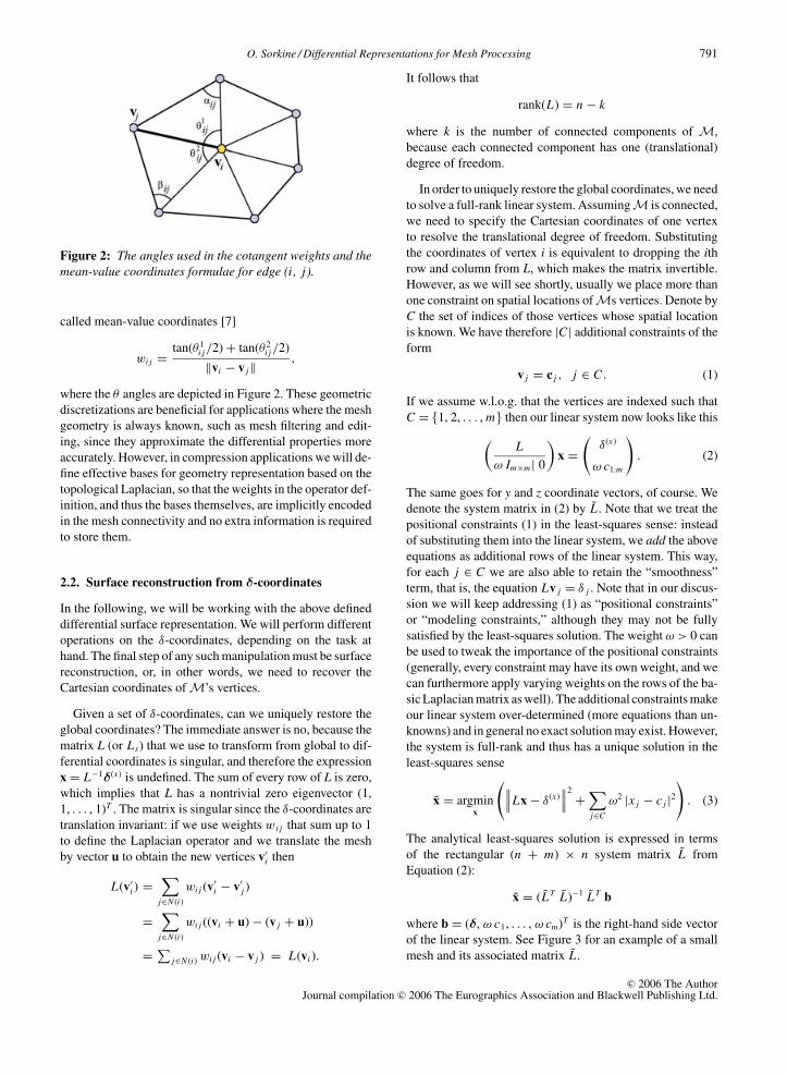
That is, Lsx = Dδ(x), Ls y = Dδ(y) and Lsz = Dδ(z), where
x is an n-vector containing the x absolute coordinates of all
the vertices and so on. See Figure 3 for an example of a mesh
and its associated matrices.
The matrix Ls (or L) is called the topological (or graph)
Laplacian of the mesh [1]. Graph Laplacians have been ex-
tensively studied in algebra and graph theory [2], primarily
because their algebraic properties are related to the combi-
natorial properties of the graphs they represent. We will look
into some of these properties later on, in Sections 2.2 and 3.
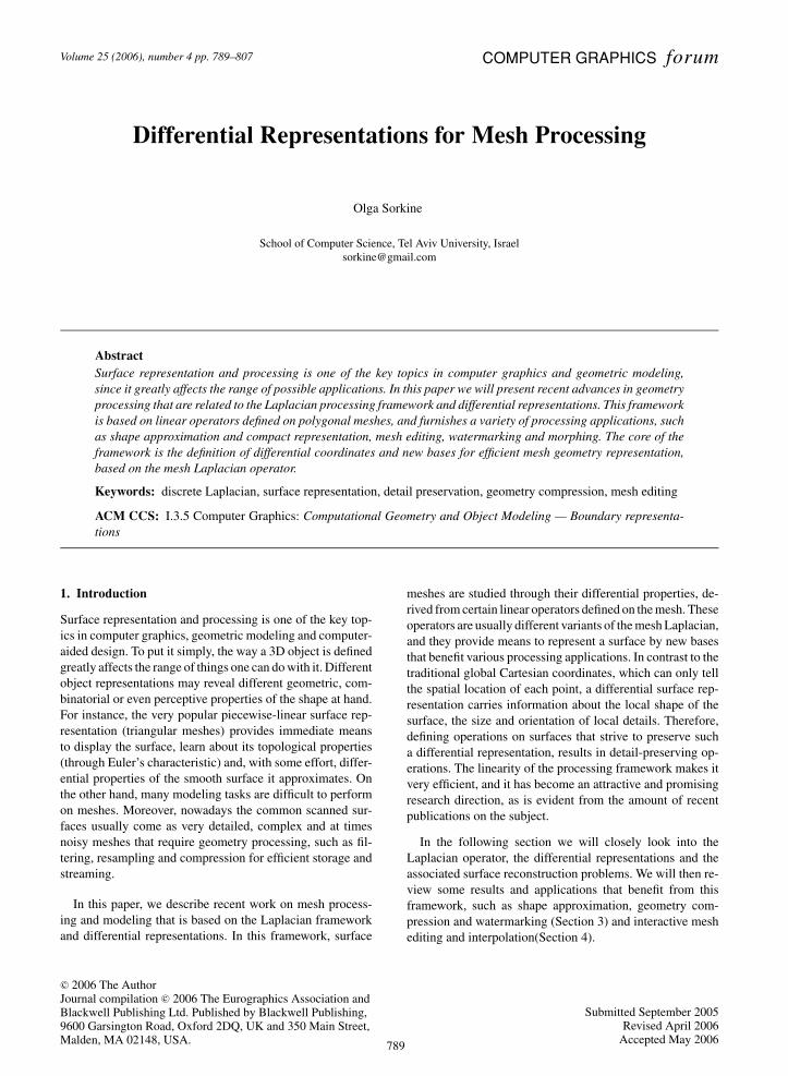
Figure 1: The vector of the differential coordinates at a ver-tex approximates the local shape characteristics of the sur-face: the normal direction and the mean curvature.
From a differential geometry perspective, the δ-
coordinates can be viewed as a discretization of the con-
tinuous Laplace–Beltrami operator [3], if we assume that our
mesh M is a piecewise-linear approximation of a smooth
surface. We can write the differential coordinate vector at
vertex vi as
δi = 1
di
∑j∈N (i)
(vi − v j ).
The sum above is a discretization of the following curvilinear
integral: 1|γ |
∫v∈γ
(vi − v) dl(v), where γ is a closed simple
surface curve around vi and |γ | is the length of γ . It is known
from differential geometry that
lim|γ |→0
1
|γ |∫
v∈γ
(vi − v) dl(v) = −H (vi ) ni
where H (vi ) is the mean curvature at vi and ni is the surface
normal. Therefore, the direction of the differential coordinate
vector approximates the local normal direction and the mag-
nitude approximates a quantity proportional to the local mean
curvature [4] (the normal scaled by the mean curvature is
termed mean-curvature normal). Intuitively, this means that
the δ-coordinates encapsulate the local surface shape (see
Figure 1).
It should be noted that geometric discretizations of the
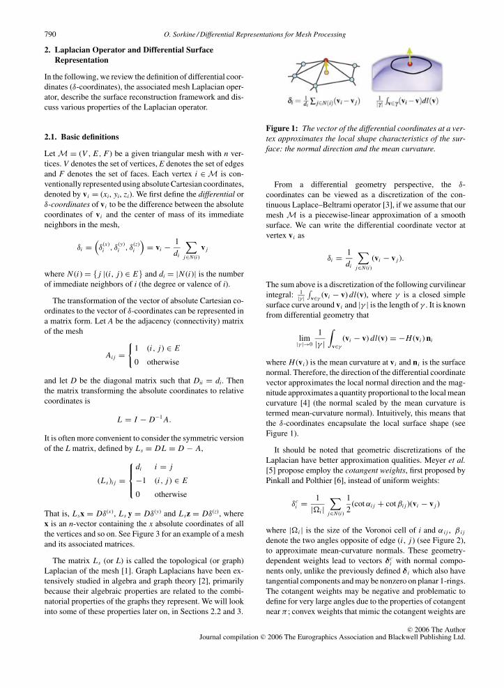
Laplacian have better approximation qualities. Meyer et al.[5] propose employ the cotangent weights, first proposed by
Pinkall and Polthier [6], instead of uniform weights:
δci = 1
|�i |∑
j∈N (i)
1
2(cot αi j + cot βi j )(vi − v j )
where |�i | is the size of the Voronoi cell of i and α i j , β i j
denote the two angles opposite of edge (i , j) (see Figure 2),
to approximate mean-curvature normals. These geometry-
dependent weights lead to vectors δci with normal compo-
nents only, unlike the previously defined δ i which also have
tangential components and may be nonzero on planar 1-rings.
The cotangent weights may be negative and problematic to
define for very large angles due to the properties of cotangent
near π ; convex weights that mimic the cotangent weights are
c© 2006 The AuthorJournal compilation c© 2006 The Eurographics Association and Blackwell Publishing Ltd.
O. Sorkine / Differential Representations for Mesh Processing 791
Figure 2: The angles used in the cotangent weights and themean-value coordinates formulae for edge (i , j ).
called mean-value coordinates [7]
wi j = tan(θ 1i j/2) + tan(θ 2
i j/2)
‖vi − v j‖ ,
where the θ angles are depicted in Figure 2. These geometric
discretizations are beneficial for applications where the mesh
geometry is always known, such as mesh filtering and edit-
ing, since they approximate the differential properties more
accurately. However, in compression applications we will de-
fine effective bases for geometry representation based on the
topological Laplacian, so that the weights in the operator def-
inition, and thus the bases themselves, are implicitly encoded
in the mesh connectivity and no extra information is required
to store them.
2.2. Surface reconstruction from δ-coordinates
In the following, we will be working with the above defined
differential surface representation. We will perform different
operations on the δ-coordinates, depending on the task at
hand. The final step of any such manipulation must be surface
reconstruction, or, in other words, we need to recover the
Cartesian coordinates of M’s vertices.
Given a set of δ-coordinates, can we uniquely restore the
global coordinates? The immediate answer is no, because the
matrix L (or Ls) that we use to transform from global to dif-
ferential coordinates is singular, and therefore the expression
x = L−1δ(x) is undefined. The sum of every row of L is zero,
which implies that L has a nontrivial zero eigenvector (1,
1, . . . , 1)T . The matrix is singular since the δ-coordinates are
translation invariant: if we use weights w i j that sum up to 1
to define the Laplacian operator and we translate the mesh
by vector u to obtain the new vertices v′i then
L(v′i ) =
∑j∈N (i)
wi j (v′i − v′
j )
=∑
j∈N (i)
wi j ((vi + u) − (v j + u))
= ∑j∈N (i) wi j (vi − v j ) = L(vi ).
It follows that
rank(L) = n − k
where k is the number of connected components of M,
because each connected component has one (translational)
degree of freedom.
In order to uniquely restore the global coordinates, we need
to solve a full-rank linear system. AssumingM is connected,
we need to specify the Cartesian coordinates of one vertex
to resolve the translational degree of freedom. Substituting
the coordinates of vertex i is equivalent to dropping the ithrow and column from L, which makes the matrix invertible.
However, as we will see shortly, usually we place more than
one constraint on spatial locations of Ms vertices. Denote by
C the set of indices of those vertices whose spatial location
is known. We have therefore |C | additional constraints of the
form
v j = c j , j ∈ C . (1)
If we assume w.l.o.g. that the vertices are indexed such that
C = {1, 2, . . . , m} then our linear system now looks like this(L
ω Im×m | 0
)x =
(δ(x)
ω c1:m
). (2)
The same goes for y and z coordinate vectors, of course. We
denote the system matrix in (2) by L . Note that we treat the
positional constraints (1) in the least-squares sense: instead
of substituting them into the linear system, we add the above
equations as additional rows of the linear system. This way,
for each j ∈ C we are also able to retain the “smoothness”
term, that is, the equation Lv j = δ j . Note that in our discus-
sion we will keep addressing (1) as “positional constraints”
or “modeling constraints,” although they may not be fully
satisfied by the least-squares solution. The weight ω > 0 can
be used to tweak the importance of the positional constraints
(generally, every constraint may have its own weight, and we
can furthermore apply varying weights on the rows of the ba-
sic Laplacian matrix as well). The additional constraints make
our linear system over-determined (more equations than un-
knowns) and in general no exact solution may exist. However,
the system is full-rank and thus has a unique solution in the
least-squares sense
x = argminx
(∥∥∥Lx − δ(x)∥∥∥2
+∑j∈C
ω2 |x j − c j |2)
. (3)
The analytical least-squares solution is expressed in terms
of the rectangular (n + m) × n system matrix L from
Equation (2):
x = (LT L)−1 LT b
where b = (δ, ω c1, . . . , ω cm)T is the right-hand side vector
of the linear system. See Figure 3 for an example of a small
mesh and its associated matrix L .
c© 2006 The AuthorJournal compilation c© 2006 The Eurographics Association and Blackwell Publishing Ltd.
792 O. Sorkine / Differential Representations for Mesh Processing
Figure 3: A small example of a triangular mesh and its as-sociated Ls matrix (top right). Second row: a 2-anchor in-vertible Laplacian and a 2-anchor L matrix. The anchors aredenoted in the mesh by red.
An important practical aspect of surface reconstruction
from δ-coordinates is the availability of efficient and accurate
numerical methods for solving the least-squares problem (3).
A recent comparative study [8] shows that direct methods
prove to be superior for these types of problems on mod-
erately sized meshes (up to a few hundreds of thousands of
vertices). The system (3) can be solved by applying Cholesky
factorization to the associated normal equations
(LT L) x = LT δ.
The matrix L is sparse, and M = LT L is also sparse (al-
though not as sparse as L) and positive definite. By using
fill-reducing reordering, it is possible to compute a sparseCholesky factorization of M
M = RT R
where R is an upper-triangular sparse matrix. The factoriza-
tion is computed once, and we can solve for several mesh
functions (x, y and z) by back substitution
RT ξ = LT δ(x)
R x = ξ.
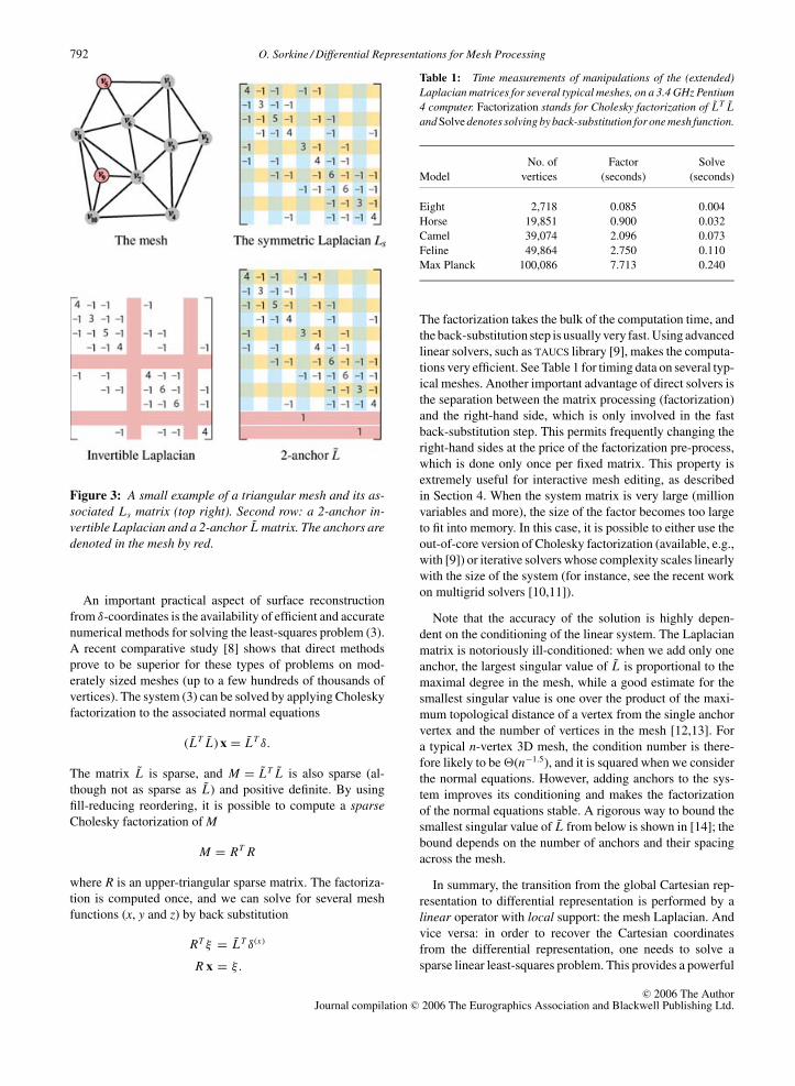
Table 1: Time measurements of manipulations of the (extended)Laplacian matrices for several typical meshes, on a 3.4 GHz Pentium4 computer. Factorization stands for Cholesky factorization of LT Land Solve denotes solving by back-substitution for one mesh function.
No. of Factor Solve
Model vertices (seconds) (seconds)
Eight 2,718 0.085 0.004
Horse 19,851 0.900 0.032
Camel 39,074 2.096 0.073
Feline 49,864 2.750 0.110
Max Planck 100,086 7.713 0.240
The factorization takes the bulk of the computation time, and
the back-substitution step is usually very fast. Using advanced
linear solvers, such as TAUCS library [9], makes the computa-
tions very efficient. See Table 1 for timing data on several typ-
ical meshes. Another important advantage of direct solvers is
the separation between the matrix processing (factorization)
and the right-hand side, which is only involved in the fast
back-substitution step. This permits frequently changing the
right-hand sides at the price of the factorization pre-process,
which is done only once per fixed matrix. This property is
extremely useful for interactive mesh editing, as described
in Section 4. When the system matrix is very large (million
variables and more), the size of the factor becomes too large
to fit into memory. In this case, it is possible to either use the
out-of-core version of Cholesky factorization (available, e.g.,
with [9]) or iterative solvers whose complexity scales linearly
with the size of the system (for instance, see the recent work
on multigrid solvers [10,11]).
Note that the accuracy of the solution is highly depen-
dent on the conditioning of the linear system. The Laplacian
matrix is notoriously ill-conditioned: when we add only one
anchor, the largest singular value of L is proportional to the
maximal degree in the mesh, while a good estimate for the
smallest singular value is one over the product of the maxi-
mum topological distance of a vertex from the single anchor
vertex and the number of vertices in the mesh [12,13]. For
a typical n-vertex 3D mesh, the condition number is there-
fore likely to be �(n−1.5), and it is squared when we consider
the normal equations. However, adding anchors to the sys-
tem improves its conditioning and makes the factorization
of the normal equations stable. A rigorous way to bound the
smallest singular value of L from below is shown in [14]; the
bound depends on the number of anchors and their spacing
across the mesh.
In summary, the transition from the global Cartesian rep-
resentation to differential representation is performed by a
linear operator with local support: the mesh Laplacian. And
vice versa: in order to recover the Cartesian coordinates
from the differential representation, one needs to solve a
sparse linear least-squares problem. This provides a powerful
c© 2006 The AuthorJournal compilation c© 2006 The Eurographics Association and Blackwell Publishing Ltd.
O. Sorkine / Differential Representations for Mesh Processing 793
framework for surface manipulation: we will apply different
modifications to the differential coordinates (such as quan-
tization for compression purposes) and/or pose additional
modeling constraints, and then reconstruct the surface by
solving the least-squares problem. The advantages of this
framework can be summarized as follows:� It strives to preserve local surface detail as much as pos-
sible under the constraints.� The least-squares solution smoothly distributes the error
across the entire domain, providing a graceful reconstruc-
tion.� Sparse linear systems can be solved very efficiently.
2.3. Spectral properties
Let us consider the Ls matrix, since it is symmetric and thus
simpler to analyze. The matrix Ls is symmetric positive semi-
definite and thus has an orthonormal eigenbasis
E = {e1, e2, . . . , en}.Denote the eigenvalues by λi ,
0 = λ1 < λ2 ≤ λ3 ≤ · · · ≤ λn .
It is known that the first nonzero λi are very small, and the
largest eigenvalue λn is bounded by the largest vertex va-
lence in M times 2. The first eigenvectors (corresponding
to small eigenvalues) are smooth, slowly varying functions
on the mesh, and the last eigenvectors have high frequency
(rapid oscillations). For example, the first eigenvector e1 is
the constant vector, that is, the “smoothest” mesh function
that does not vary at all. In fact, the Laplacian eigenbasis is
an extension of the discrete Fourier basis to irregular domains
[4]. The eigenvalues are considered as mesh-frequencies. We
will see in the following how this fact is exploited for sig-
nal processing on meshes, compact geometry representation,
watermarking and more. See also [16] for an earlier state-of-
the-art report on this subject.
3. Efficient Shape Representation
In this section we review several methods for efficient and
compact geometry representation that benefit from the mesh
Laplacian operator and the framework presented in Section 2.
For an extensive recent survey on general compression meth-
ods, we refer the reader to [17].
3.1. Efficient bases for geometry representation
Finding a good basis for compact shape representation means
that one can use only a fraction of the basis functions to ap-
proximate a given geometry well. This idea is extensively
used in signal processing and in the image domain, by defin-
ing Fourier or wavelet bases. The regular 1D and 2D settings
are well studied in both continuous and discrete settings, and
the sampling theorem tells us the number of basis functions
we need to use for perfect signal reconstruction. Things are
more involved for the irregular setting of arbitrary triangu-
lar meshes. One possible approach of direct application of
the signal processing theory on meshes is to first perform
semi-regular remeshing by parameterizing the mesh over a
simple base complex, and then apply variations of 2D signal
processing methods [18,19,20,21,22]. Another possibility is,
instead of altering the mesh, to work directly on the irreg-
ular mesh and develop generalizations of the methods from
regular settings.
Karni and Gotsman [15] introduce a spectral method where
the mesh is approximated by reconstructing its geometry us-
ing a linear combination of a number of basis vectors. The
basis is the spectral basis E of the Ls matrix, which can be
regarded as a generalization of the discrete Fourier basis (see
Section 2.3). Similarly to JPEG compression of images, the
mesh geometry functions x, y, z are decomposed in the basis
E:
x = α1 e1 + α2 e2 + · · · + αn en (4)
and the high-frequency components (coefficients of the last
eigenvectors) are truncated. The coefficients α i are quantized
and subsequently entropy coded. It is assumed that the mesh
connectivity is known to the decoder prior to receiving the
geometry coefficients, so that the decoder first computes the
spectral basis and then reconstructs the geometry by combin-
ing the coefficients. Note that this method is readily made for
progressive streaming, since if one sends the α i coefficients in
ascending order of i, the decoder can first reconstruct a coarse
(very smooth) approximation of the geometry, and then grad-
ually add high-frequency detail, as more coefficients become
available.
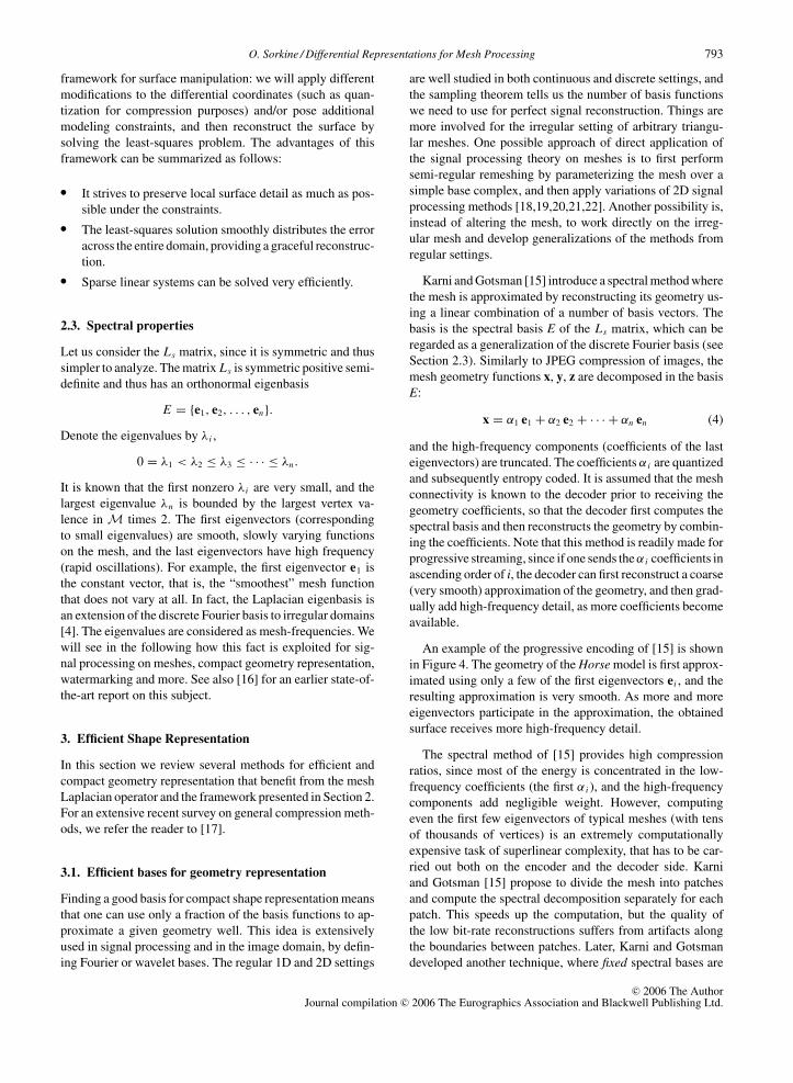
An example of the progressive encoding of [15] is shown
in Figure 4. The geometry of the Horse model is first approx-
imated using only a few of the first eigenvectors ei , and the
resulting approximation is very smooth. As more and more
eigenvectors participate in the approximation, the obtained
surface receives more high-frequency detail.
The spectral method of [15] provides high compression
ratios, since most of the energy is concentrated in the low-
frequency coefficients (the first α i ), and the high-frequency
components add negligible weight. However, computing
even the first few eigenvectors of typical meshes (with tens
of thousands of vertices) is an extremely computationally
expensive task of superlinear complexity, that has to be car-
ried out both on the encoder and the decoder side. Karni
and Gotsman [15] propose to divide the mesh into patches
and compute the spectral decomposition separately for each
patch. This speeds up the computation, but the quality of
the low bit-rate reconstructions suffers from artifacts along
the boundaries between patches. Later, Karni and Gotsman
developed another technique, where fixed spectral bases are
c© 2006 The AuthorJournal compilation c© 2006 The Eurographics Association and Blackwell Publishing Ltd.
794 O. Sorkine / Differential Representations for Mesh Processing
Figure 4: Progressive approximations of the Horse geometry using the eigenvectors of the topological Laplacian [15]. The leftfigure shows an approximation using only a small number of the first eigenvectors (those that correspond to small eigenvalues).When more eigenvectors are added to the approximation, the surface attains more high-frequency detail (middle and right).Data courtesy of Zachi Karni.
employed [23]. The spectral basis of a regular mesh with
n vertices is used to approximate the Laplacian eigenbasis,
and the computational cost of spectral analysis is avoided on
the decoder side altogether. Of course, this technique works
better for meshes that are close to being regular.
In [24,25], a different class of shape approximation tech-
niques for irregular triangular meshes was introduced. The
method approximates the geometry of the mesh using a lin-
ear combination of a small number of basis vectors that are
functions of the mesh connectivity and of the mesh indices
of a number of anchor vertices. The initial motivation was
to improve the shortcomings of the spectral basis [15]. One
must bear in mind that, together with their appealing proper-
ties, the spectral bases are geometry-oblivious, since the basis
vectors are functions of the connectivity alone. In contrast, the
new geometry-aware method derives the basis both from the
mesh connectivity and geometry. The basis vectors in [25] are
centered around selected “geometrically important” anchor
vertices. This allows a terse capturing of important features of
the surface and leads to compact and efficient representation
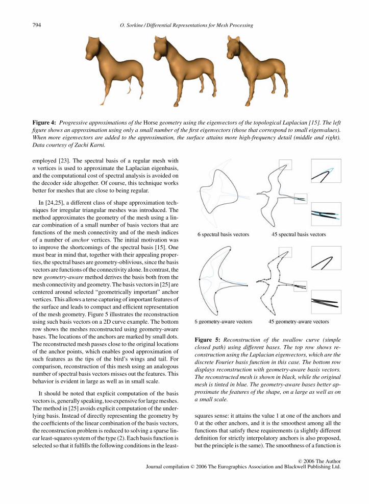
of the mesh geometry. Figure 5 illustrates the reconstruction
using such basis vectors on a 2D curve example. The bottom
row shows the meshes reconstructed using geometry-aware
bases. The locations of the anchors are marked by small dots.
The reconstructed mesh passes close to the original locations
of the anchor points, which enables good approximation of
such features as the tips of the bird’s wings and tail. For
comparison, reconstruction of this mesh using an analogous
number of spectral basis vectors misses out the features. This
behavior is evident in large as well as in small scale.
It should be noted that explicit computation of the basis
vectors is, generally speaking, too expensive for large meshes.
The method in [25] avoids explicit computation of the under-
lying basis. Instead of directly representing the geometry by
the coefficients of the linear combination of the basis vectors,
the reconstruction problem is reduced to solving a sparse lin-
ear least-squares system of the type (2). Each basis function is
selected so that it fulfills the following conditions in the least-
Figure 5: Reconstruction of the swallow curve (simpleclosed path) using different bases. The top row shows re-construction using the Laplacian eigenvectors, which are thediscrete Fourier basis function in this case. The bottom rowdisplays reconstruction with geometry-aware basis vectors.The reconstructed mesh is shown in black, while the originalmesh is tinted in blue. The geometry-aware bases better ap-proximate the features of the shape, on a large as well as ona small scale.
squares sense: it attains the value 1 at one of the anchors and
0 at the other anchors, and it is the smoothest among all the
functions that satisfy these requirements (a slightly different
definition for strictly interpolatory anchors is also proposed,
but the principle is the same). The smoothness of a function is
c© 2006 The AuthorJournal compilation c© 2006 The Eurographics Association and Blackwell Publishing Ltd.
O. Sorkine / Differential Representations for Mesh Processing 795
0 50 100 150 200 250 300−0.6
−0.4
−0.2
0
0.2
0.4
0.6
0.8
1
1.25 first vectors out of 5 anchor vectors
0 50 100 150 200 250 300−0.4
−0.2
0
0.2
0.4
0.6
0.8
1
1.25 first vectors out of 20 anchor vectors
(a) (b)
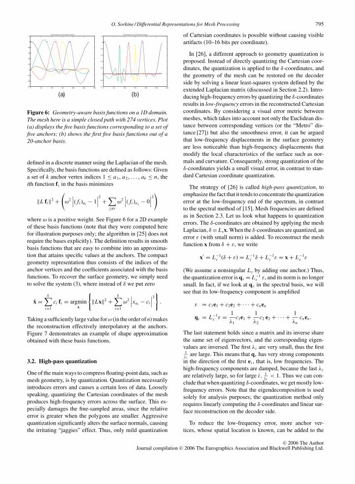
Figure 6: Geometry-aware basis functions on a 1D domain.The mesh here is a simple closed path with 274 vertices. Plot(a) displays the five basis functions corresponding to a set offive anchors; (b) shows the first five basis functions out of a20-anchor basis.
defined in a discrete manner using the Laplacian of the mesh.
Specifically, the basis functions are defined as follows: Given
a set of k anchor vertex indices 1 ≤ a1, a2, . . . , ak ≤ n, the
ith function fi in the basis minimizes
‖L fi‖2 +(
ω2∣∣∣( fi )ai − 1
∣∣∣2
+∑j �=i
ω2∣∣∣( fi )a j − 0
∣∣∣2
)
where ω is a positive weight. See Figure 6 for a 2D example
of these basis functions (note that they were computed here
for illustration purposes only; the algorithm in [25] does not
require the bases explicitly). The definition results in smooth
basis functions that are easy to combine into an approxima-
tion that attains specific values at the anchors. The compact
geometry representation thus consists of the indices of the
anchor vertices and the coefficients associated with the basis
functions. To recover the surface geometry, we simply need
to solve the system (3), where instead of δ we put zero
x =k∑
i=1
ci fi = argminx
{‖Lx‖2 +
k∑i=1
ω2∣∣∣xai − ci
∣∣∣2
}.
Taking a sufficiently large value forω (in the order of n) makes
the reconstruction effectively interpolatory at the anchors.
Figure 7 demonstrates an example of shape approximation
obtained with these basis functions.
3.2. High-pass quantization
One of the main ways to compress floating-point data, such as
mesh geometry, is by quantization. Quantization necessarily
introduces errors and causes a certain loss of data. Loosely
speaking, quantizing the Cartesian coordinates of the mesh
produces high-frequency errors across the surface. This es-
pecially damages the fine-sampled areas, since the relative
error is greater when the polygons are smaller. Aggressive
quantization significantly alters the surface normals, causing
the irritating “jaggies” effect. Thus, only mild quantization
of Cartesian coordinates is possible without causing visible
artifacts (10–16 bits per coordinate).
In [26], a different approach to geometry quantization is
proposed. Instead of directly quantizing the Cartesian coor-
dinates, the quantization is applied to the δ-coordinates, and
the geometry of the mesh can be restored on the decoder
side by solving a linear least-squares system defined by the
extended Laplacian matrix (discussed in Section 2.2). Intro-
ducing high-frequency errors by quantizing the δ-coordinates
results in low-frequency errors in the reconstructed Cartesian
coordinates. By considering a visual error metric between
meshes, which takes into account not only the Euclidean dis-
tance between corresponding vertices (or the “Metro” dis-
tance [27]) but also the smoothness error, it can be argued
that low-frequency displacements in the surface geometry
are less noticeable than high-frequency displacements that
modify the local characteristics of the surface such as nor-
mals and curvature. Consequently, strong quantization of the
δ-coordinates yields a small visual error, in contrast to stan-
dard Cartesian coordinate quantization.
The strategy of [26] is called high-pass quantization, to
emphasize the fact that it tends to concentrate the quantization
error at the low-frequency end of the spectrum, in contrast
to the spectral method of [15]. Mesh frequencies are defined
as in Section 2.3. Let us look what happens to quantization
errors. The δ-coordinates are obtained by applying the mesh
Laplacian, δ = Lsx. When the δ-coordinates are quantized, an
error ε (with small norm) is added. To reconstruct the mesh
function x from δ + ε, we write
x′ = L−1s (δ + ε) = L−1
s δ + L−1s ε = x + L−1
s ε
(We assume a nonsingular Ls by adding one anchor.) Thus,
the quantization error is qε = L−1s ε, and its norm is no longer
small. In fact, if we look at qε in the spectral basis, we will
see that its low-frequency component is amplified
ε = c1e1 + c2e2 + · · · + cnen
qε = L−1s ε = 1
λ1
c1e1 + 1
λ2
c2 e2 + · · · + 1
λncnen .
The last statement holds since a matrix and its inverse share
the same set of eigenvectors, and the corresponding eigen-
values are inversed. The first λi are very small, thus the first1λi
are large. This means that qε has very strong components
in the direction of the first ei , that is, low frequencies. The
high-frequency components are damped, because the last λi
are relatively large, so for large i, 1λi
< 1. Thus we can con-
clude that when quantizing δ-coordinates, we get mostly low-
frequency errors. Note that the eigendecomposition is used
solely for analysis purposes; the quantization method only
requires linearly computing the δ-coordinates and linear sur-
face reconstruction on the decoder side.
To reduce the low-frequency error, more anchor ver-
tices, whose spatial location is known, can be added to the
c© 2006 The AuthorJournal compilation c© 2006 The Eurographics Association and Blackwell Publishing Ltd.
796 O. Sorkine / Differential Representations for Mesh Processing
Figure 7: Reconstruction of the Feline model using an increasing number of geometry-aware basis vectors. The sizes of theencoded geometry files are displayed below the models. The letter e denotes the L2 error value, given in units of 10−4.
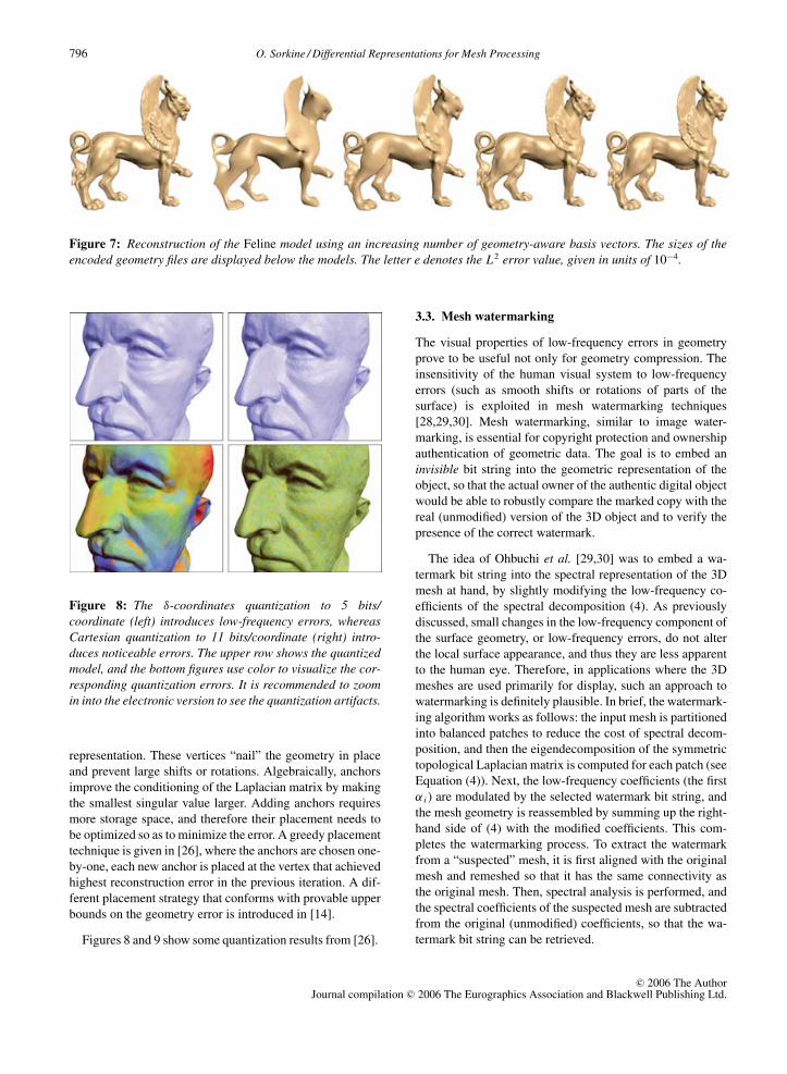
Figure 8: The δ-coordinates quantization to 5 bits/coordinate (left) introduces low-frequency errors, whereasCartesian quantization to 11 bits/coordinate (right) intro-duces noticeable errors. The upper row shows the quantizedmodel, and the bottom figures use color to visualize the cor-responding quantization errors. It is recommended to zoomin into the electronic version to see the quantization artifacts.
representation. These vertices “nail” the geometry in place
and prevent large shifts or rotations. Algebraically, anchors
improve the conditioning of the Laplacian matrix by making
the smallest singular value larger. Adding anchors requires
more storage space, and therefore their placement needs to
be optimized so as to minimize the error. A greedy placement
technique is given in [26], where the anchors are chosen one-
by-one, each new anchor is placed at the vertex that achieved
highest reconstruction error in the previous iteration. A dif-
ferent placement strategy that conforms with provable upper
bounds on the geometry error is introduced in [14].
Figures 8 and 9 show some quantization results from [26].
3.3. Mesh watermarking
The visual properties of low-frequency errors in geometry
prove to be useful not only for geometry compression. The
insensitivity of the human visual system to low-frequency
errors (such as smooth shifts or rotations of parts of the
surface) is exploited in mesh watermarking techniques
[28,29,30]. Mesh watermarking, similar to image water-
marking, is essential for copyright protection and ownership
authentication of geometric data. The goal is to embed an
invisible bit string into the geometric representation of the
object, so that the actual owner of the authentic digital object
would be able to robustly compare the marked copy with the
real (unmodified) version of the 3D object and to verify the
presence of the correct watermark.
The idea of Ohbuchi et al. [29,30] was to embed a wa-
termark bit string into the spectral representation of the 3D
mesh at hand, by slightly modifying the low-frequency co-
efficients of the spectral decomposition (4). As previously
discussed, small changes in the low-frequency component of
the surface geometry, or low-frequency errors, do not alter
the local surface appearance, and thus they are less apparent
to the human eye. Therefore, in applications where the 3D
meshes are used primarily for display, such an approach to
watermarking is definitely plausible. In brief, the watermark-
ing algorithm works as follows: the input mesh is partitioned
into balanced patches to reduce the cost of spectral decom-
position, and then the eigendecomposition of the symmetric
topological Laplacian matrix is computed for each patch (see
Equation (4)). Next, the low-frequency coefficients (the first
α i ) are modulated by the selected watermark bit string, and
the mesh geometry is reassembled by summing up the right-
hand side of (4) with the modified coefficients. This com-
pletes the watermarking process. To extract the watermark
from a “suspected” mesh, it is first aligned with the original
mesh and remeshed so that it has the same connectivity as
the original mesh. Then, spectral analysis is performed, and
the spectral coefficients of the suspected mesh are subtracted
from the original (unmodified) coefficients, so that the wa-
termark bit string can be retrieved.
c© 2006 The AuthorJournal compilation c© 2006 The Eurographics Association and Blackwell Publishing Ltd.
O. Sorkine / Differential Representations for Mesh Processing 797
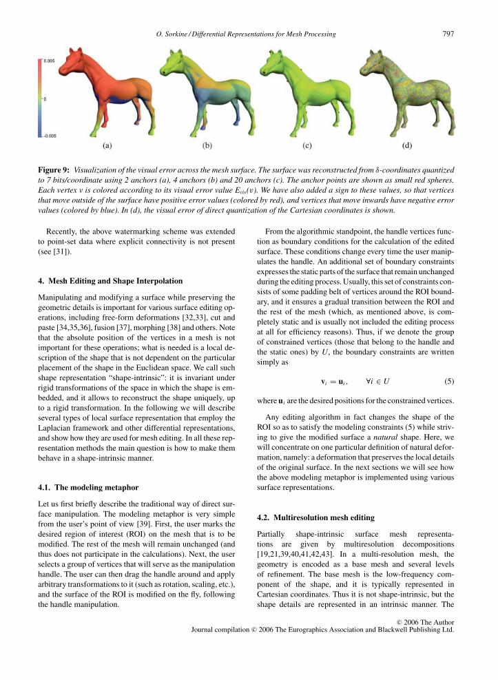
Figure 9: Visualization of the visual error across the mesh surface. The surface was reconstructed from δ-coordinates quantizedto 7 bits/coordinate using 2 anchors (a), 4 anchors (b) and 20 anchors (c). The anchor points are shown as small red spheres.Each vertex v is colored according to its visual error value Evis(v). We have also added a sign to these values, so that verticesthat move outside of the surface have positive error values (colored by red), and vertices that move inwards have negative errorvalues (colored by blue). In (d), the visual error of direct quantization of the Cartesian coordinates is shown.
Recently, the above watermarking scheme was extended
to point-set data where explicit connectivity is not present
(see [31]).
4. Mesh Editing and Shape Interpolation
Manipulating and modifying a surface while preserving the
geometric details is important for various surface editing op-
erations, including free-form deformations [32,33], cut and
paste [34,35,36], fusion [37], morphing [38] and others. Note
that the absolute position of the vertices in a mesh is not
important for these operations; what is needed is a local de-
scription of the shape that is not dependent on the particular
placement of the shape in the Euclidean space. We call such
shape representation “shape-intrinsic”: it is invariant under
rigid transformations of the space in which the shape is em-
bedded, and it allows to reconstruct the shape uniquely, up
to a rigid transformation. In the following we will describe
several types of local surface representation that employ the
Laplacian framework and other differential representations,
and show how they are used for mesh editing. In all these rep-
resentation methods the main question is how to make them
behave in a shape-intrinsic manner.
4.1. The modeling metaphor
Let us first briefly describe the traditional way of direct sur-
face manipulation. The modeling metaphor is very simple
from the user’s point of view [39]. First, the user marks the
desired region of interest (ROI) on the mesh that is to be
modified. The rest of the mesh will remain unchanged (and
thus does not participate in the calculations). Next, the user
selects a group of vertices that will serve as the manipulation
handle. The user can then drag the handle around and apply
arbitrary transformations to it (such as rotation, scaling, etc.),
and the surface of the ROI is modified on the fly, following
the handle manipulation.
From the algorithmic standpoint, the handle vertices func-
tion as boundary conditions for the calculation of the edited
surface. These conditions change every time the user manip-
ulates the handle. An additional set of boundary constraints
expresses the static parts of the surface that remain unchanged
during the editing process. Usually, this set of constraints con-
sists of some padding belt of vertices around the ROI bound-
ary, and it ensures a gradual transition between the ROI and
the rest of the mesh (which, as mentioned above, is com-
pletely static and is usually not included the editing process
at all for efficiency reasons). Thus, if we denote the group
of constrained vertices (those that belong to the handle and
the static ones) by U, the boundary constraints are written
simply as
vi = ui , ∀i ∈ U (5)
where ui are the desired positions for the constrained vertices.
Any editing algorithm in fact changes the shape of the
ROI so as to satisfy the modeling constraints (5) while striv-
ing to give the modified surface a natural shape. Here, we
will concentrate on one particular definition of natural defor-
mation, namely: a deformation that preserves the local details
of the original surface. In the next sections we will see how
the above modeling metaphor is implemented using various
surface representations.
4.2. Multiresolution mesh editing
Partially shape-intrinsic surface mesh representa-
tions are given by multiresolution decompositions
[19,21,39,40,41,42,43]. In a multi-resolution mesh, the
geometry is encoded as a base mesh and several levels
of refinement. The base mesh is the low-frequency com-
ponent of the shape, and it is typically represented in
Cartesian coordinates. Thus it is not shape-intrinsic, but the
shape details are represented in an intrinsic manner. The
c© 2006 The AuthorJournal compilation c© 2006 The Eurographics Association and Blackwell Publishing Ltd.
798 O. Sorkine / Differential Representations for Mesh Processing
refinements are described locally, so that the geometric
details are mostly captured in a discrete set of translation-
and rotation-invariant coordinates. Using this representation,
modeling operations can be performed on an appropriate
user-specified level-of-detail. The multiresolution hierarchy
can be constructed for both the connectivity and the
geometry (as in, e.g., [19,21]), or the only geometry (as
in, e.g., [39,42,43]), where the connectivity of the mesh
remains full and unchanged in all the levels-of-detail in the
hierarchy. Different levels of refinement are usually obtained
by gradual smoothing of the mesh.
We will outline the editing mechanism of the multireso-
lution framework of Kobbelt and colleagues [39,41,43] as
an exemplary multiresolution technique that also uses the
Laplacian framework. For simplicity, let us assume that the
mesh hierarchy consists of two levels only, sharing the same
connectivity: the smooth base mesh and the detailed mesh.
The detailed level is encoded with respect to the base level
by computing the offset of each vertex and representing this
offset in the local frame of the corresponding vertex in the
base mesh. The choice of the local frames is rotation- and
translation-invariant, and therefore the representation of the
offsets (which are, in fact, the surface details in this case)
is independent of the location of the mesh in space. Mesh
editing is performed as follows: first, the smooth base mesh
is deformed according to the constraints (5); then the local
frames are recomputed on the deformed base mesh, and fi-
nally, the original detail offsets (in their local frame represen-
tation) are added to the base mesh. This way, the local details
are reproduced correctly in the deformed mesh: for example,
if the surface was bent, the local frames of the smooth base
mesh rotate, and thus so do the offsets. This key concept of
invariance in local representation is illustrated in Figure 10.
How is the base mesh deformed? It is assumed that the base
mesh is smooth enough and does not contain local details that
need to be preserved. Therefore, the base mesh is deformed
by solving an optimization problem with two objectives:
(i) satisfying the user constraints (5) and (ii) keeping the
surface of the base mesh smooth. The latter goal is achieved
by describing smoothness in terms of the mesh Laplacian op-
erator, as we already saw in Section 3.1. Botsch and Kobbelt
[43] propose different orders of smoothness, obtained via dif-
ferent orders of the Laplacian operator. The optimization is
formulated as
Lkx = 0
leading to C k−1 smoothness of the resulting surface. Proba-
bly the most common value is k = 2, producing the so-called
“thin-plate” surface. The Equations (5) are incorporated as
hard constraints into the above system by substitution, secur-
ing its nontrivial solution. When k = 2, this optimization is
equivalent to solving the least-squares problem (3) where all
the δ-coordinates are set to zero and sufficiently large weight
is put on the positional constraints, to effectively make them
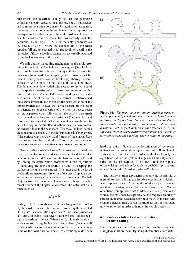
Figure 10: The importance of rotation-invariant represen-tation. (a) the original shape, where the base shape is drawnin brown. In (b), the base shape was bent, while the detailswere encoded in a rotation-invariant manner, and thus theirorientation with respect to the base was preserved. In (c), thesame deformation leads to distorted orientation of the details(stretch) because the encoding was not rotation-invariant.
hard constraints. Note that the factorization of the system
matrix can be computed once per choice of ROI and handle
vertices; each time the user transforms the handle, only the
right-hand side of the system changes and thus only a back-
substitution step is required. This allows interactive response
of the editing mechanism for fairly large ROIs (up to several
tens of thousands of vertices, refer to Table 1).
The multiresolution approach is probably the most intuitive
method for mesh editing, and its advantage is the straightfor-
ward representation of the details of the shape in a man-
ner that is invariant to the global coordinate system. On the
other hand, this approach defines details explicitly, or in other
words, one may need to explicitly set the required amount of
smoothing to create a satisfactory base mesh. In meshes with
complex details, many levels of multi-resolution hierarchy
may be required in order to handle the details correctly.
4.3. Single-resolution local representations
for mesh editing
Local details can be defined in a more implicit way with
a single-resolution mesh, by using differential coordinates.
c© 2006 The AuthorJournal compilation c© 2006 The Eurographics Association and Blackwell Publishing Ltd.
O. Sorkine / Differential Representations for Mesh Processing 799
Mesh editing using this representation was pioneered by
Alexa [44]. The basic idea is simply to add the positional
constraints (5) to the system that reconstructs the Cartesian
coordinates of the mesh from the differential coordinates (3).
Once again, note that the system matrix needs to be con-
structed and factored only once per choice of ROI and handle;
during user manipulation one only needs to solve the linear
system by back-substitution, which is very efficient.
The above idea for surface representation and reconstruc-
tion was further elaborated in [45,46,47]. Yu et al. [47] in-
troduce a technique called Poisson Editing, formulated by
manipulation of the gradients of the coordinate functions
(x , y, z) of the mesh. The surface is reconstructed by solv-
ing the least-squares system resulting from discretizing the
Poisson equation
∇2 f = � f = ∇ · w (6)
with Dirichlet boundary conditions. Here, f is the unknown
scalar function on the mesh, that is, one of the coordinate
functions x , y, z of the deformed mesh. The vector field w
is the gradient field of the corresponding original coordi-
nate function. The set of boundary constraints consists of
both positional constraints of the form (5) and constraints
on the gradients of the handle vertices, directly expressed by
the desired linear transformation on the handle. The spatial
Laplacian operator �, restricted to the mesh, is discretized
using the cotangent weights. By inspecting Equation (6), we
can see that it has a similar form to the Laplacian surface re-
construction system (3); the difference lies on the right-hand
side, that is expressed in terms of a vector field rather than a
scalar field, and the constraints are substituted into the system
(so that this is not a least-squares optimization).
In [45], the surface is reconstructed from the Laplacian
δ-coordinates of the mesh and spatial boundary conditions
by solving (3). Both Lipman et al. [45] and Yu et al. [47]
point out the main problem of the above approach: the need
to rotate the local frames that define the Laplacians, or the gra-
dients, to correctly handle the orientation of the local details.
If this issue is not properly addressed, the system in (3) (or in
(6)), tries to preserve the Laplacian vectors (or the gradients)
in their original orientation with respect to the global coor-
dinate system. Therefore a result in the spirit of the sketch in
Figure 10c would be obtained.
Yu et al. and Lipman et al. propose remedy to this prob-
lem by explicit assignment of the local rotations. Lipman
et al. [45] estimate the local rotations of the frames on the
underlying smooth surface by smoothing the “naive” solu-
tion of (3); then the original Laplacians are rotated by these
estimated rotations and the reconstruction system is solved
again. This heuristic achieves good results on meshes with
relatively small details; applying it to complex meshes where
the details are far from being height-fields above a smooth
base surface would require a lot of smoothing iterations. An
important feature of this approach is that it deduces the lo-
cal rotations based on translational, or positional constraints
alone; the user is not expected to provide rotational trans-
formations of the handle. So even in the simplest case of
grabbing one handle vertex and “pulling” it out of the sur-
face, the technique will produce rotation estimates for the
surface details and they will be transformed accordingly.
Yu et al. [47] propagate the rotation (or any other linear
transformation) of the editing handle, defined by the user, to
all the gradient vectors of the ROI. This is the major differ-
ence from [45], because here the user is expected to specify
compatible translation and rotation constraints on the han-
dle; translational constraints alone will result in no local
rotations (and thus the surface details may be significantly
distorted). The propagated transformations are interpolated
with the identity, where the interpolation weight for each tri-
angle is proportional to the geodesic distance of the triangle
from the handle. As pointed out in [48], this solution may also
produce unexpected results for meshes with complex features
protruding from the smooth base surface. This is because the
tip of a protruding feature is geodesically further from the
handle than the vertices around the feature’s base, and thus
the tip receives a smaller share of the deformation than the
base (whereas for a natural result, it should be roughly the
same amount of deformation).
A different interpolation scheme for deformation propa-
gation was recently proposed by Zayer et al. [49]: it avoids
geodesics computation, creating a harmonic scalar field on
the mesh instead. The harmonic field attains the value of 1
at the handle vertices and 0 at the boundary of the ROI, and
varies monotonically on the rest of the ROI, thus providing a
valid and smoother alternative to the geodesic weights. The
harmonic field is obtained by solving (2), only the 1 and 0
constraints are substituted into the system rather than added in
least-squares sense. An additional advantage of this approach
is that it uses the same system matrix both for the computation
of the weights and for the actual editing (only with different
right-hand sides), thus the factorization of the matrix serves
both tasks at once. As a side note, we mention that the mesh
Laplacian operator is tightly coupled with Hodge theory and
computation of globally conformal (harmonic) mesh param-
eterizations for arbitrary topology. This topic is outside of
the scope of this paper; the reader is kindly referred to recent
publications [6,50,51,52] for further information.
It is important to note that all the above-mentioned methods
[45,47,49] are fast: the size of the system matrices involved in
the reconstruction is n × n, where n is the number of vertices
in the ROI. This size will grow in the follow-up works, as we
will see shortly.
Subsequent research continued to look for truly shape-
intrinsic representation suitable for mesh editing. Sheffer and
Kraevoy [53] introduced the so-called pyramid coordinates:
at each vertex i of the mesh, the normal and the tangential
components of the local frame are stored, independently of
c© 2006 The AuthorJournal compilation c© 2006 The Eurographics Association and Blackwell Publishing Ltd.
800 O. Sorkine / Differential Representations for Mesh Processing
the global coordinate frame. To construct this representa-
tion, a local projection plane is fitted to the vertices of the
1-ring by averaging the face normals of the 1-ring. The nor-
mal component of the center vertex i is its distance to the
projection plane, whereas the tangential component is en-
coded as the edge lengths and the angles between the edges
of the 1-ring, projected onto the plane. Since this representa-
tion is evidently rotation-invariant, it allows performing nat-
ural and large deformations on meshes based on translational
(or other) constraints on the handle, as well as linear blend
between different shapes (given the correspondence between
them). However, the reconstruction of the Cartesian coor-
dinates from the pyramid coordinates is clearly a nonlinear
optimization (involving cross-product and norm computa-
tions to construct the projection planes), which makes it time
consuming.
In [46], the Laplacian editing method that implicitly trans-
forms the differential δ-coordinates is proposed, based on
finding an optimal transform for each vertex. The editing
paradigm implies positional constraints on some vertices,
and it deduces the local rotations based on translations of the
handle, similarly to [45]. The local transforms are defined
by comparing 1-rings in the original mesh and the unknown
deformed mesh, and are formulated as linear expressions in
the vertices of the unknown mesh. The reconstruction Equa-
tion (3) is thus altered to make the differential coordinates
similarity-invariant: we solve for the reconstructed geometry
V ′ = {v′1, . . . , v′
n} by minimizing
E(V ′) =n∑
i=1
∥∥Ti (V′)δi − L(v′
i )∥∥2 +
∑i∈U
‖v′i − ui‖2 (7)
where U is the set of constrained vertices. The transforma-
tions Ti are themselves unknowns that linearly depend on the
unknown vertices V ′. Each Ti is a transformation that takes
the original 1-ring of vertex i to the newly reconstructed one
Ti = argminTi
∑j∈{i} ⋃
N (i)
‖Ti v j − v′j‖2
In addition, the Ti’s are constrained to be translations, rota-
tions and scales only, in order to enforce local detail preserva-
tion and to disallow shears. In 2D, this is easy since similarity
transformations have linear form
Ti =
⎛⎜⎝ s −h tx
h s ty
0 0 1
⎞⎟⎠In 3D, however, a linearized version of rotation constraint is
needed, since true 3D rotation matrices cannot be expressed
linearly in 3D. If h represents the rotation axis and H is
the skew-symmetric matrix such that Hx = h × x, ∀x ∈ R3,
then the class of translations, rotations and scales has the form
s exp H = s(α I + β H + γ hT h).
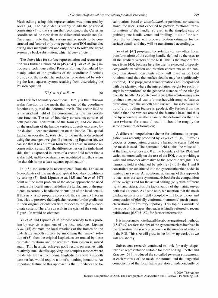
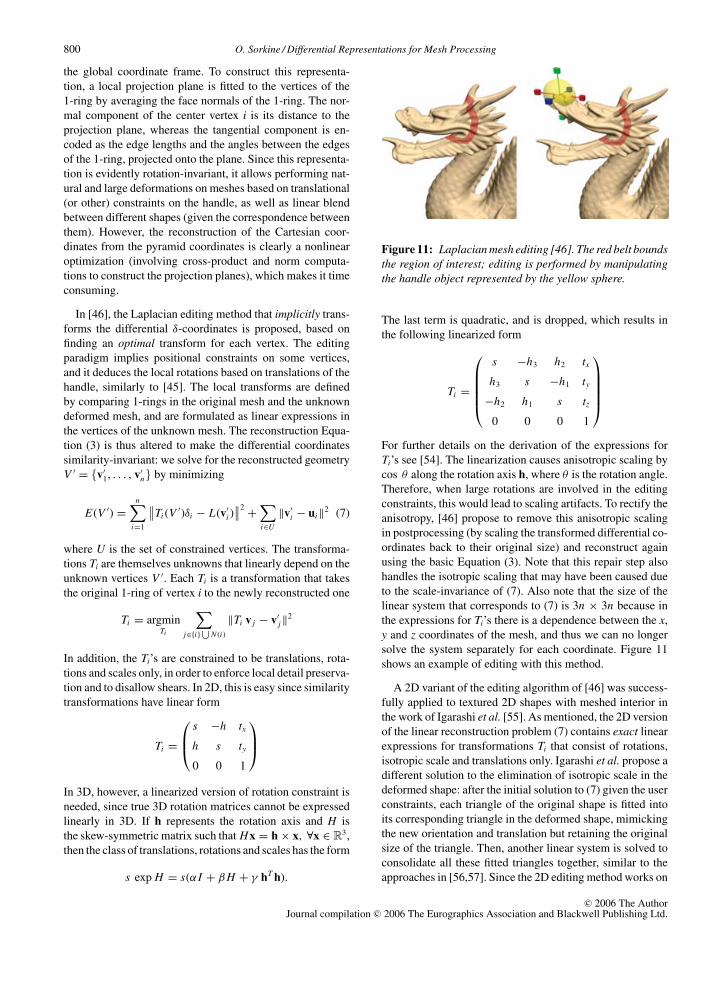
Figure 11: Laplacian mesh editing [46]. The red belt boundsthe region of interest; editing is performed by manipulatingthe handle object represented by the yellow sphere.
The last term is quadratic, and is dropped, which results in
the following linearized form
Ti =
⎛⎜⎜⎜⎜⎝s −h3 h2 tx
h3 s −h1 ty
−h2 h1 s tz
0 0 0 1
⎞⎟⎟⎟⎟⎠For further details on the derivation of the expressions for
Ti’s see [54]. The linearization causes anisotropic scaling by
cos θ along the rotation axis h, where θ is the rotation angle.
Therefore, when large rotations are involved in the editing
constraints, this would lead to scaling artifacts. To rectify the
anisotropy, [46] propose to remove this anisotropic scaling
in postprocessing (by scaling the transformed differential co-
ordinates back to their original size) and reconstruct again
using the basic Equation (3). Note that this repair step also
handles the isotropic scaling that may have been caused due
to the scale-invariance of (7). Also note that the size of the
linear system that corresponds to (7) is 3n × 3n because in
the expressions for Ti’s there is a dependence between the x,
y and z coordinates of the mesh, and thus we can no longer
solve the system separately for each coordinate. Figure 11
shows an example of editing with this method.
A 2D variant of the editing algorithm of [46] was success-
fully applied to textured 2D shapes with meshed interior in
the work of Igarashi et al. [55]. As mentioned, the 2D version
of the linear reconstruction problem (7) contains exact linear
expressions for transformations Ti that consist of rotations,
isotropic scale and translations only. Igarashi et al. propose a
different solution to the elimination of isotropic scale in the
deformed shape: after the initial solution to (7) given the user
constraints, each triangle of the original shape is fitted into
its corresponding triangle in the deformed shape, mimicking
the new orientation and translation but retaining the original
size of the triangle. Then, another linear system is solved to
consolidate all these fitted triangles together, similar to the
approaches in [56,57]. Since the 2D editing method works on
c© 2006 The AuthorJournal compilation c© 2006 The Eurographics Association and Blackwell Publishing Ltd.
O. Sorkine / Differential Representations for Mesh Processing 801
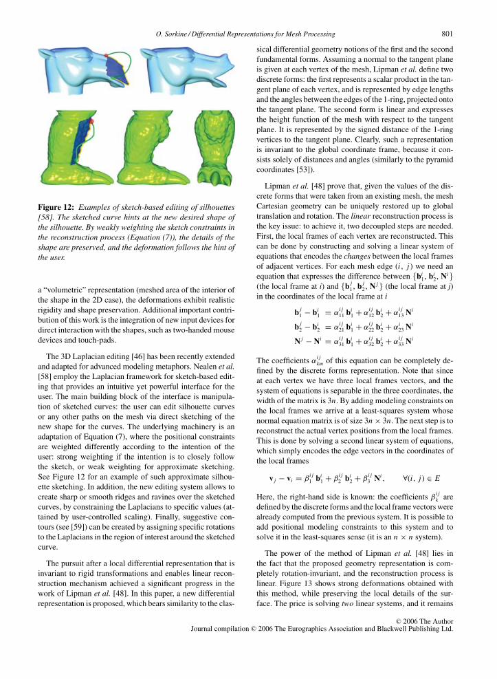
Figure 12: Examples of sketch-based editing of silhouettes[58]. The sketched curve hints at the new desired shape ofthe silhouette. By weakly weighting the sketch constraints inthe reconstruction process (Equation (7)), the details of theshape are preserved, and the deformation follows the hint ofthe user.
a “volumetric” representation (meshed area of the interior of
the shape in the 2D case), the deformations exhibit realistic
rigidity and shape preservation. Additional important contri-
bution of this work is the integration of new input devices for
direct interaction with the shapes, such as two-handed mouse
devices and touch-pads.
The 3D Laplacian editing [46] has been recently extended
and adapted for advanced modeling metaphors. Nealen et al.[58] employ the Laplacian framework for sketch-based edit-
ing that provides an intuitive yet powerful interface for the
user. The main building block of the interface is manipula-
tion of sketched curves: the user can edit silhouette curves
or any other paths on the mesh via direct sketching of the
new shape for the curves. The underlying machinery is an
adaptation of Equation (7), where the positional constraints
are weighted differently according to the intention of the
user: strong weighting if the intention is to closely follow
the sketch, or weak weighting for approximate sketching.
See Figure 12 for an example of such approximate silhou-
ette sketching. In addition, the new editing system allows to
create sharp or smooth ridges and ravines over the sketched
curves, by constraining the Laplacians to specific values (at-
tained by user-controlled scaling). Finally, suggestive con-
tours (see [59]) can be created by assigning specific rotations
to the Laplacians in the region of interest around the sketched
curve.
The pursuit after a local differential representation that is
invariant to rigid transformations and enables linear recon-
struction mechanism achieved a significant progress in the
work of Lipman et al. [48]. In this paper, a new differential
representation is proposed, which bears similarity to the clas-
sical differential geometry notions of the first and the second
fundamental forms. Assuming a normal to the tangent plane
is given at each vertex of the mesh, Lipman et al. define two
discrete forms: the first represents a scalar product in the tan-
gent plane of each vertex, and is represented by edge lengths
and the angles between the edges of the 1-ring, projected onto
the tangent plane. The second form is linear and expresses
the height function of the mesh with respect to the tangent
plane. It is represented by the signed distance of the 1-ring
vertices to the tangent plane. Clearly, such a representation
is invariant to the global coordinate frame, because it con-
sists solely of distances and angles (similarly to the pyramid
coordinates [53]).
Lipman et al. [48] prove that, given the values of the dis-
crete forms that were taken from an existing mesh, the mesh
Cartesian geometry can be uniquely restored up to global
translation and rotation. The linear reconstruction process is
the key issue: to achieve it, two decoupled steps are needed.
First, the local frames of each vertex are reconstructed. This
can be done by constructing and solving a linear system of
equations that encodes the changes between the local frames
of adjacent vertices. For each mesh edge (i , j) we need an
equation that expresses the difference between {bi1, bi
2, Ni}(the local frame at i) and {b
j1, b
j2, N j} (the local frame at j)
in the coordinates of the local frame at i
bj1 − bi
1 = αi j11 bi
1 + αi j12 bi
2 + αi j13 Ni
bj2 − bi
2 = αi j21 bi
1 + αi j22 bi
2 + αi23 Ni
N j − Ni = αi j31 bi
1 + αi j32 bi
2 + αi j33 Ni
The coefficients αi jkm of this equation can be completely de-
fined by the discrete forms representation. Note that since
at each vertex we have three local frames vectors, and the
system of equations is separable in the three coordinates, the
width of the matrix is 3n. By adding modeling constraints on
the local frames we arrive at a least-squares system whose
normal equation matrix is of size 3n × 3n. The next step is to
reconstruct the actual vertex positions from the local frames.
This is done by solving a second linear system of equations,
which simply encodes the edge vectors in the coordinates of
the local frames
v j − vi = βi j1 bi
1 + βi j2 bi
2 + βi j3 Ni , ∀(i, j) ∈ E
Here, the right-hand side is known: the coefficients βi jk are
defined by the discrete forms and the local frame vectors were
already computed from the previous system. It is possible to
add positional modeling constraints to this system and to
solve it in the least-squares sense (it is an n × n system).
The power of the method of Lipman et al. [48] lies in
the fact that the proposed geometry representation is com-
pletely rotation-invariant, and the reconstruction process is
linear. Figure 13 shows strong deformations obtained with
this method, while preserving the local details of the sur-
face. The price is solving two linear systems, and it remains
c© 2006 The AuthorJournal compilation c© 2006 The Eurographics Association and Blackwell Publishing Ltd.
802 O. Sorkine / Differential Representations for Mesh Processing
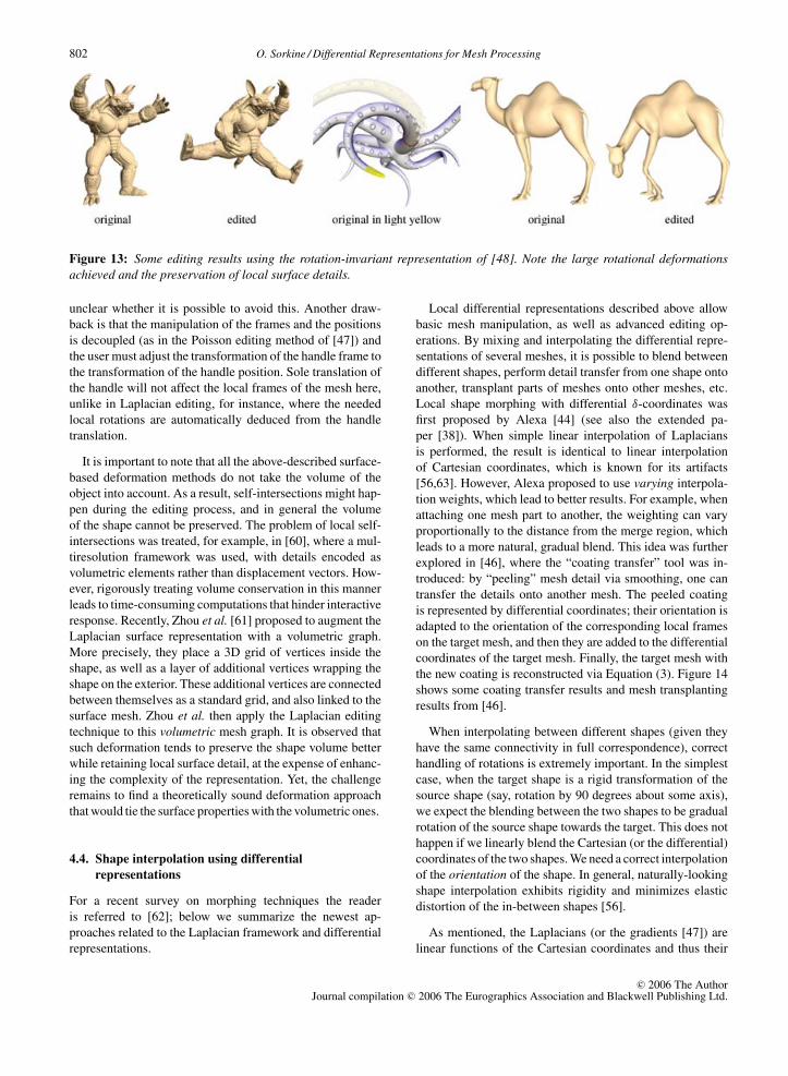
Figure 13: Some editing results using the rotation-invariant representation of [48]. Note the large rotational deformationsachieved and the preservation of local surface details.
unclear whether it is possible to avoid this. Another draw-
back is that the manipulation of the frames and the positions
is decoupled (as in the Poisson editing method of [47]) and
the user must adjust the transformation of the handle frame to
the transformation of the handle position. Sole translation of
the handle will not affect the local frames of the mesh here,
unlike in Laplacian editing, for instance, where the needed
local rotations are automatically deduced from the handle
translation.
It is important to note that all the above-described surface-
based deformation methods do not take the volume of the
object into account. As a result, self-intersections might hap-
pen during the editing process, and in general the volume
of the shape cannot be preserved. The problem of local self-
intersections was treated, for example, in [60], where a mul-
tiresolution framework was used, with details encoded as
volumetric elements rather than displacement vectors. How-
ever, rigorously treating volume conservation in this manner
leads to time-consuming computations that hinder interactive
response. Recently, Zhou et al. [61] proposed to augment the
Laplacian surface representation with a volumetric graph.
More precisely, they place a 3D grid of vertices inside the
shape, as well as a layer of additional vertices wrapping the
shape on the exterior. These additional vertices are connected
between themselves as a standard grid, and also linked to the
surface mesh. Zhou et al. then apply the Laplacian editing
technique to this volumetric mesh graph. It is observed that
such deformation tends to preserve the shape volume better
while retaining local surface detail, at the expense of enhanc-
ing the complexity of the representation. Yet, the challenge
remains to find a theoretically sound deformation approach
that would tie the surface properties with the volumetric ones.
4.4. Shape interpolation using differential
representations
For a recent survey on morphing techniques the reader
is referred to [62]; below we summarize the newest ap-
proaches related to the Laplacian framework and differential
representations.
Local differential representations described above allow
basic mesh manipulation, as well as advanced editing op-
erations. By mixing and interpolating the differential repre-
sentations of several meshes, it is possible to blend between
different shapes, perform detail transfer from one shape onto
another, transplant parts of meshes onto other meshes, etc.
Local shape morphing with differential δ-coordinates was
first proposed by Alexa [44] (see also the extended pa-
per [38]). When simple linear interpolation of Laplacians
is performed, the result is identical to linear interpolation
of Cartesian coordinates, which is known for its artifacts
[56,63]. However, Alexa proposed to use varying interpola-
tion weights, which lead to better results. For example, when
attaching one mesh part to another, the weighting can vary
proportionally to the distance from the merge region, which
leads to a more natural, gradual blend. This idea was further
explored in [46], where the “coating transfer” tool was in-
troduced: by “peeling” mesh detail via smoothing, one can
transfer the details onto another mesh. The peeled coating
is represented by differential coordinates; their orientation is
adapted to the orientation of the corresponding local frames
on the target mesh, and then they are added to the differential
coordinates of the target mesh. Finally, the target mesh with
the new coating is reconstructed via Equation (3). Figure 14
shows some coating transfer results and mesh transplanting
results from [46].
When interpolating between different shapes (given they
have the same connectivity in full correspondence), correct
handling of rotations is extremely important. In the simplest
case, when the target shape is a rigid transformation of the
source shape (say, rotation by 90 degrees about some axis),
we expect the blending between the two shapes to be gradual
rotation of the source shape towards the target. This does not
happen if we linearly blend the Cartesian (or the differential)
coordinates of the two shapes. We need a correct interpolation
of the orientation of the shape. In general, naturally-looking
shape interpolation exhibits rigidity and minimizes elastic
distortion of the in-between shapes [56].
As mentioned, the Laplacians (or the gradients [47]) are
linear functions of the Cartesian coordinates and thus their
c© 2006 The AuthorJournal compilation c© 2006 The Eurographics Association and Blackwell Publishing Ltd.
O. Sorkine / Differential Representations for Mesh Processing 803
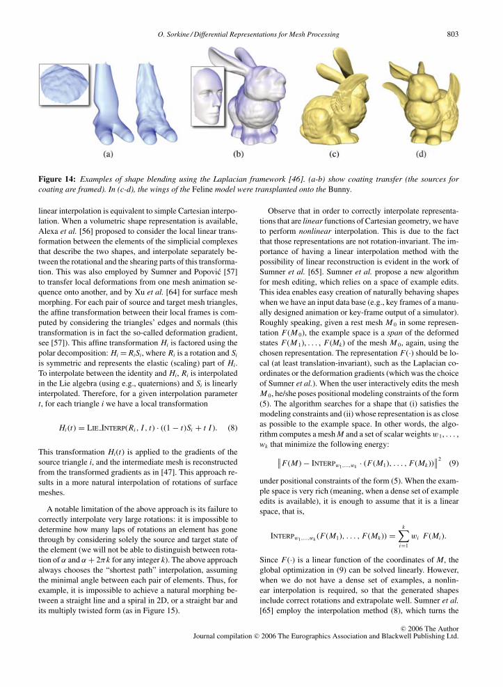
Figure 14: Examples of shape blending using the Laplacian framework [46]. (a-b) show coating transfer (the sources forcoating are framed). In (c-d), the wings of the Feline model were transplanted onto the Bunny.
linear interpolation is equivalent to simple Cartesian interpo-
lation. When a volumetric shape representation is available,
Alexa et al. [56] proposed to consider the local linear trans-
formation between the elements of the simplicial complexes
that describe the two shapes, and interpolate separately be-
tween the rotational and the shearing parts of this transforma-
tion. This was also employed by Sumner and Popovic [57]
to transfer local deformations from one mesh animation se-
quence onto another, and by Xu et al. [64] for surface mesh
morphing. For each pair of source and target mesh triangles,
the affine transformation between their local frames is com-
puted by considering the triangles’ edges and normals (this
transformation is in fact the so-called deformation gradient,
see [57]). This affine transformation Hi is factored using the
polar decomposition: Hi = RiSi, where Ri is a rotation and Si
is symmetric and represents the elastic (scaling) part of Hi.
To interpolate between the identity and Hi, Ri is interpolated
in the Lie algebra (using e.g., quaternions) and Si is linearly
interpolated. Therefore, for a given interpolation parameter
t, for each triangle i we have a local transformation
Hi (t) = LIE INTERP(Ri , I , t) · ((1 − t)Si + t I ). (8)
This transformation Hi(t) is applied to the gradients of the
source triangle i, and the intermediate mesh is reconstructed
from the transformed gradients as in [47]. This approach re-
sults in a more natural interpolation of rotations of surface
meshes.
A notable limitation of the above approach is its failure to
correctly interpolate very large rotations: it is impossible to
determine how many laps of rotations an element has gone
through by considering solely the source and target state of
the element (we will not be able to distinguish between rota-
tion of α and α + 2πk for any integer k). The above approach
always chooses the “shortest path” interpolation, assuming
the minimal angle between each pair of elements. Thus, for
example, it is impossible to achieve a natural morphing be-
tween a straight line and a spiral in 2D, or a straight bar and
its multiply twisted form (as in Figure 15).
Observe that in order to correctly interpolate representa-
tions that are linear functions of Cartesian geometry, we have
to perform nonlinear interpolation. This is due to the fact
that those representations are not rotation-invariant. The im-
portance of having a linear interpolation method with the
possibility of linear reconstruction is evident in the work of
Sumner et al. [65]. Sumner et al. propose a new algorithm
for mesh editing, which relies on a space of example edits.
This idea enables easy creation of naturally behaving shapes
when we have an input data base (e.g., key frames of a manu-
ally designed animation or key-frame output of a simulator).
Roughly speaking, given a rest mesh M 0 in some represen-
tation F(M 0), the example space is a span of the deformed
states F(M 1), . . . , F(Mk) of the mesh M 0, again, using the
chosen representation. The representation F(·) should be lo-
cal (at least translation-invariant), such as the Laplacian co-
ordinates or the deformation gradients (which was the choice
of Sumner et al.). When the user interactively edits the mesh
M 0, he/she poses positional modeling constraints of the form
(5). The algorithm searches for a shape that (i) satisfies the
modeling constraints and (ii) whose representation is as close
as possible to the example space. In other words, the algo-
rithm computes a mesh M and a set of scalar weights w1, . . . ,
wk that minimize the following energy:∥∥F(M) − INTERPw1,...,wk · (F(M1), . . . , F(Mk))∥∥2
(9)
under positional constraints of the form (5). When the exam-
ple space is very rich (meaning, when a dense set of example
edits is available), it is enough to assume that it is a linear
space, that is,
INTERPw1,...,wk (F(M1), . . . , F(Mk)) =k∑
i=1
wi F(Mi ).
Since F(·) is a linear function of the coordinates of M, the
global optimization in (9) can be solved linearly. However,
when we do not have a dense set of examples, a nonlin-
ear interpolation is required, so that the generated shapes
include correct rotations and extrapolate well. Sumner et al.[65] employ the interpolation method (8), which turns the
c© 2006 The AuthorJournal compilation c© 2006 The Eurographics Association and Blackwell Publishing Ltd.
804 O. Sorkine / Differential Representations for Mesh Processing
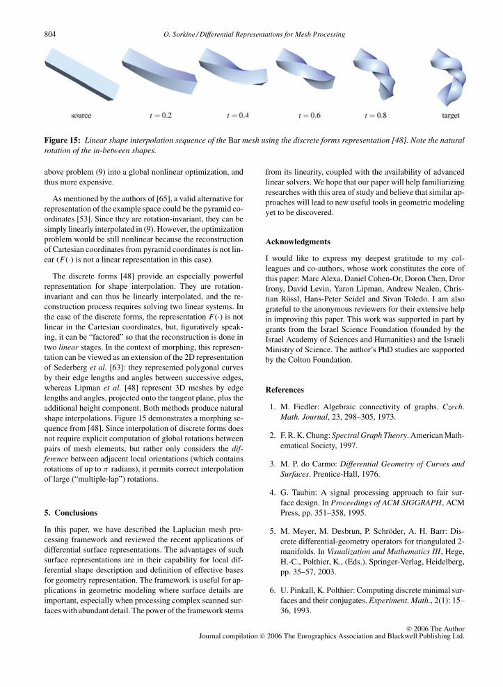
Figure 15: Linear shape interpolation sequence of the Bar mesh using the discrete forms representation [48]. Note the naturalrotation of the in-between shapes.
above problem (9) into a global nonlinear optimization, and
thus more expensive.
As mentioned by the authors of [65], a valid alternative for
representation of the example space could be the pyramid co-
ordinates [53]. Since they are rotation-invariant, they can be
simply linearly interpolated in (9). However, the optimization
problem would be still nonlinear because the reconstruction
of Cartesian coordinates from pyramid coordinates is not lin-
ear (F(·) is not a linear representation in this case).
The discrete forms [48] provide an especially powerful
representation for shape interpolation. They are rotation-
invariant and can thus be linearly interpolated, and the re-
construction process requires solving two linear systems. In
the case of the discrete forms, the representation F(·) is not
linear in the Cartesian coordinates, but, figuratively speak-
ing, it can be “factored” so that the reconstruction is done in
two linear stages. In the context of morphing, this represen-
tation can be viewed as an extension of the 2D representation
of Sederberg et al. [63]: they represented polygonal curves
by their edge lengths and angles between successive edges,
whereas Lipman et al. [48] represent 3D meshes by edge
lengths and angles, projected onto the tangent plane, plus the
additional height component. Both methods produce natural
shape interpolations. Figure 15 demonstrates a morphing se-
quence from [48]. Since interpolation of discrete forms does
not require explicit computation of global rotations between
pairs of mesh elements, but rather only considers the dif-ference between adjacent local orientations (which contains
rotations of up to π radians), it permits correct interpolation
of large (“multiple-lap”) rotations.
5. Conclusions
In this paper, we have described the Laplacian mesh pro-
cessing framework and reviewed the recent applications of
differential surface representations. The advantages of such
surface representations are in their capability for local dif-
ferential shape description and definition of effective bases
for geometry representation. The framework is useful for ap-
plications in geometric modeling where surface details are
important, especially when processing complex scanned sur-
faces with abundant detail. The power of the framework stems
from its linearity, coupled with the availability of advanced
linear solvers. We hope that our paper will help familiarizing
researches with this area of study and believe that similar ap-
proaches will lead to new useful tools in geometric modeling
yet to be discovered.
Acknowledgments
I would like to express my deepest gratitude to my col-
leagues and co-authors, whose work constitutes the core of
this paper: Marc Alexa, Daniel Cohen-Or, Doron Chen, Dror
Irony, David Levin, Yaron Lipman, Andrew Nealen, Chris-
tian Rossl, Hans-Peter Seidel and Sivan Toledo. I am also
grateful to the anonymous reviewers for their extensive help
in improving this paper. This work was supported in part by
grants from the Israel Science Foundation (founded by the
Israel Academy of Sciences and Humanities) and the Israeli
Ministry of Science. The author’s PhD studies are supported
by the Colton Foundation.
References
1. M. Fiedler: Algebraic connectivity of graphs. Czech.Math. Journal, 23, 298–305, 1973.
2. F. R. K. Chung: Spectral Graph Theory. American Math-
ematical Society, 1997.
3. M. P. do Carmo: Differential Geometry of Curves andSurfaces. Prentice-Hall, 1976.
4. G. Taubin: A signal processing approach to fair sur-
face design. In Proceedings of ACM SIGGRAPH, ACM
Press, pp. 351–358, 1995.
5. M. Meyer, M. Desbrun, P. Schroder, A. H. Barr: Dis-
crete differential-geometry operators for triangulated 2-
manifolds. In Visualization and Mathematics III, Hege,
H.-C., Polthier, K., (Eds.). Springer-Verlag, Heidelberg,
pp. 35–57, 2003.
6. U. Pinkall, K. Polthier: Computing discrete minimal sur-
faces and their conjugates. Experiment. Math., 2(1): 15–
36, 1993.
c© 2006 The AuthorJournal compilation c© 2006 The Eurographics Association and Blackwell Publishing Ltd.
O. Sorkine / Differential Representations for Mesh Processing 805
7. M. S. Floater: Mean value coordinates. CAGD, 20(1):
19–27, 2003.
8. M. Botsch, D. Bommes, L. Kobbelt: Efficient linear sys-
tem solvers for mesh processing. IMA Mathematics ofSurfaces XI, Lecture Notes in Computer Science, 3604:
62–83, 2005.
9. S. Toledo: Taucs: A Library of Sparse Linear Solvers,version 2.2. Tel-Aviv University, Available online at
http://www.tau.ac.il/∼stoledo/taucs/, Sept. 2003.
10. B. Aksoylu, A. Khodakovsky, P. Schroder: Multilevel
solvers for unstructured surface meshes. SISC, 26(4):
1146–1165, 2005.
11. L. Shi, Y. Yu, N. Bell, W.-W. Feng: A fast multigrid
algorithm for mesh deformation. In Proceedings of ACMSIGGRAPH, To appear, 2006.
12. E. G. Boman, B. Hendrickson: Support theory for pre-
conditioning. SIAM Journal on Matrix Analysis and Ap-plications, 25(3): 694–717, 2003.
13. S. Guattery, G. L. Miller: Graph embeddings and Lapla-
cian eigenvalues. SIAM Journal on Matrix Analysis andApplications, 21(3): 703–723, 2000.
14. D. Chen, D. Cohen-Or, O. Sorkine, S. Toledo: Algebraic
analysis of high-pass quantization. ACM Transactions onGraphics, 24(4): 1259–1282, 2005.
15. Z. Karni, C. Gotsman: Spectral compression of mesh
geometry. In Proceedings of ACM SIGGRAPH, pp. 279–
286, 2000.
16. G. Taubin: Geometric signal processing on polygonal
meshes. In Proceedings of Eurographics (STAR volume),State of the Art Report, 2000.
17. P. Alliez, C. Gotsman: Recent advances in compression
of 3D meshes. In Advances in Multiresolution for Geo-metric Modelling, Dodgson, N., Floater, M., Sabin, M.,
(Eds.), Springer-Verlag, pp. 3–26, 2005.
18. M. Eck, T. DeRose, T. Duchamp, H. Hoppe, M. Louns-
bery, W. Stuetzle: Multiresolution analysis of arbitrary
meshes. In Proceedings of ACM SIGGRAPH, pp. 173–
182, 1995.
19. D. Zorin, P. Schroder, W. Sweldens: Interactive mul-
tiresolution mesh editing. In Proceedings of ACM SIG-GRAPH, pp. 259–268, 1997.
20. A. W. F. Lee, W. Sweldens, P. Schroder, L. Cowsar, D.
Dobkin: MAPS: Multiresolution adaptive parameteriza-
tion of surfaces. In Proceedings of ACM SIGGRAPH,
ACM Press, pp. 95–104, 1998.
21. I. Guskov, W. Sweldens, P. Schroder: Multiresolution
signal processing for meshes. In Proceedings of ACMSIGGRAPH, ACM Press, pp. 325–334, 1999.
22. A. Khodakovsky, P. Schroder, W. Sweldens: Progres-
sive geometry compression. In Proceedings of ACM SIG-GRAPH, pp. 271–278, 2000.
23. Z. Karni, C. Gotsman: 3D mesh compression using fixed
spectral bases. In Proceedings of Graphics Interface,
Canadian Information Processing Society, pp. 1–8, 2001.
24. O. Sorkine, D. Cohen-Or: Least-squares meshes. In Pro-ceedings of Shape Modeling International, IEEE Com-
puter Society Press, pp. 191–199, 2004.
25. O. Sorkine, D. Cohen-Or, D. Irony, S. Toledo:
Geometry-aware bases for shape approximation. IEEETransactions on Visualization and Computer Graphics,
11(2): 171–180, 2005.
26. O. Sorkine, D. Cohen-Or, S. Toledo: High-pass quan-
tization for mesh encoding. In Proceedings of the Eu-rographics/ACM SIGGRAPH Symposium on Geometryprocessing, Eurographics Association, pp. 42–51, 2003.
27. P. Cignoni, C. Rocchini, R. Scopigno: Metro: Measuring
error on simplified surfaces. Computer Graphics Forum,
17(2): 167–174, 1998.
28. E. Praun, H. Hoppe, A. Finkelstein: Robust mesh water-
marking. In Proceedings of ACM SIGGRAPH, pp. 49–
56, 1999.
29. R. Ohbuchi, S. Takahashi, T. Miyazawa, A. Mukaiyama:
Watermarking 3D polygonal meshes in the mesh spectral
domain. In Proceedings of Graphics Interface, Morgan
Kaufmann Publishers, pp. 9–17, (June 2001).
30. R. Ohbuchi, A. Mukaiyama, S. Takahashi: A frequency-
domain approach to watermarking 3D shapes. ComputerGraphics Forum (Proceedings of Eurographics), 21(3):
373–382, 2002.
31. D. Cotting, T. Weyrich, M. Pauly, M. Gross: Robust wa-
termarking of point-sampled geometry. In Proceedingsof Shape Modeling International, pp. 233–242, 2004.
32. T. W. Sederberg, S. R. Parry: Free-form deformation of
solid geometric models. In Proceedings of ACM SIG-GRAPH, pp. 151–160, 1986.
33. S. Coquillart: Extended free-form deformation: A sculp-
turing tool for 3D geometric modeling. In Proceedingsof ACM SIGGRAPH, 90, pp. 187–196, 1990.
34. M. Ranta, M. Inui, F. Kimura, M. Mantyla: Cut and paste
based modeling with boundary features. In SMA ’93:
c© 2006 The AuthorJournal compilation c© 2006 The Eurographics Association and Blackwell Publishing Ltd.
806 O. Sorkine / Differential Representations for Mesh Processing
Proceedings of the Second Symposium on Solid Model-ing and Applications (May 1993), pp. 303–312.
35. S. Kuriyama, T. Kaneko: Discrete parametrization for
deforming arbitrary meshes. In Proceedings of GraphicsInterface, pp. 132–139, 1999.
36. H. Biermann, I. Martin, F. Bernardini, D. Zorin: Cut-and-
paste editing of multiresolution surfaces. In Proceedingsof ACM SIGGRAPH, pp. 312–321, 2002.
37. T. Kanai, H. Suzuki, J. Mitani, F. Kimura: Interac-
tive mesh fusion based on local 3D metamorphosis. In
Proceedings of Graphics Interface, pp. 148–156, (June
1999.
38. M. Alexa: Differential coordinates for local mesh morph-
ing and deformation. The Visual Computer, 19(2): 105–
114, 2003.
39. L. Kobbelt, S. Campagna, J. Vorsatz, H.-P. Seidel: Inter-
active multi-resolution modeling on arbitrary meshes.
In Proceedings of ACM SIGGRAPH, ACM Press, pp.
105–114, 1998.
40. D. Forsey, R. Bartels: Hierarchical B-spline refinement.
In Proceedings of ACM SIGGRAPH, ACM Press, pp.
205–212, 1988.
41. L. Kobbelt, J. Vorsatz, H.-P. Seidel: Multiresolution hier-
archies on unstructured triangle meshes. ComputationalGeometry: Theory and Applications, 14: 5–24, 1999.
42. S. Lee: Interactive multiresolution editing of arbitrary
meshes. Computer Graphics Forum (Eurographics 99),18(3): 73–82, 1999.
43. M. Botsch, L. Kobbelt: An intuitive framework for real-
time freeform modeling. In Proceedings of ACM SIG-GRAPH, pp. 630–634, 2004.
44. M. Alexa: Local control for mesh morphing. In Proceed-ings of the International Conference on Shape Modelingand Applications (SMI-01) (Los Alamitos, CA, May 7–
11 2001), Werner, B. (Ed.), pp. 209–215.
45. Y. Lipman, O. Sorkine, D. Cohen-Or, D. Levin, C.
Rossl, H.-P. Seidel: Differential coordinates for inter-
active mesh editing. In Proceedings of Shape ModelingInternational, IEEE Computer Society Press, pp. 181–
190, 2004.
46. O. Sorkine, Y. Lipman, D. Cohen-Or, M. Alexa, C. Rossl,
H.-P. Seidel: Laplacian surface editing. In Proceedingsof the Eurographics/ACM SIGGRAPH Symposium onGeometry processing, ACM Press, pp. 179–188, 2004.
47. Y. Yu, K. Zhou, D. Xu, X. Shi, H. Bao, B. Guo, H.-Y.
Shum: Mesh editing with Poisson-based gradient field
manipulation. ACM Transactions on Graphics (Proceed-ings of ACM SIGGRAPH), 23(3): 644–651, 2004.
48. Y. Lipman, O. Sorkine, D. Levin, D. Cohen-Or: Linear
rotation-invariant coordinates for meshes. ACM Trans-actions on Graphics (Proceedings of ACM SIGGRAPH),24(3): 479–487, 2005.
49. R. Zayer, C. Rossl, Z. Karni, H.-P. Seidel: Harmonic
guidance for surface deformation. In Computer Graph-ics Forum (Proceedings of Eurographics), Eurographics,
Blackwell, pp. 601–609, 2005.
50. X. Gu, S.-T. Yau: Global conformal surface param-
eterization. In Proceedings of the Eurographics/ACMSIGGRAPH Symposium on Geometry processing, Eu-
rographics Association, pp. 127–137, 2003.
51. X. Ni, M. Garland, J. C. Hart: Fair morse functions for
extracting the topological structure of a surface mesh.
ACM Transactions on Graphics (Proceedings of ACMSIGGRAPH), 23(3): 613–622, 2004.
52. S. Dong, S. Kircher, M. Garland: Harmonic functions for
quadrilateral remeshing of arbitrary manifolds. CAGD,
22(5): 392–423, 2005.
53. A. Sheffer, V. Kraevoy: Pyramid coordinates for mor-
phing and deformation. In Proceedings of the SecondInternational Symposium on 3DPVT (3D Data Process-ing, Visualization, and Transmission), IEEE Computer
Society Press, pp. 68–75, 2004.
54. Y. Lipman, O. Sorkine, M. Alexa, D. Cohen-Or, D.
Levin, C. Rossl, H.-P. Seidel: Laplacian framework for
interactive mesh editing. International Journal of ShapeModeling, 11(1): 43–62, 2005.
55. T. Igarashi, T. Moscovich, J. F. Hughes: As-rigid-as-
possible shape manipulation. ACM Transactions onGraphics (Proceedings of ACM SIGGRAPH), 24(3):
1134–1141, 2005.
56. M. Alexa, D. Cohen-Or, D. Levin: As-rigid-as-possible
shape interpolation. In Proceedings of ACM SIG-GRAPH, pp. 157–164, 2000.
57. R. W. Sumner, J. Popovic: Deformation transfer for tri-
angle meshes. ACM Transactions on Graphics (Proceed-ings of ACM SIGGRAPH), 23(3): 399–405, 2004.
58. A. Nealen, O. Sorkine, M. Alexa, D. Cohen-Or: A
sketch-based interface for detail-preserving mesh edit-
ing. ACM Transactions on Graphics (Proceedings ofACM SIGGRAPH), 24(3): 1142–1147, 2005.
c© 2006 The AuthorJournal compilation c© 2006 The Eurographics Association and Blackwell Publishing Ltd.
O. Sorkine / Differential Representations for Mesh Processing 807
59. D. DeCarlo, A. Finkelstein, S. Rusinkiewicz, A. Santella:
Suggestive contours for conveying shape. ACM Trans-actions on Graphics (Proccedings of ACM SIGGRAPH),22(3): 848–855, 2003.
60. M. Botsch, L. Kobbelt: Multiresolution surface repre-
sentation based on displacement volumes. ComputerGraphics Forum, 22(3): 483–492, 2003.
61. K. Zhou, J. Huang, J. Snyder, X. Liu, H. Bao, B. Guo, H.-
Y. Shum: Large mesh deformation using the volumetric
graph Laplacian. ACM Transactions on Graphics (Pro-ceedings of ACM SIGGRAPH), 24(3): 496–503, 2005.
62. M. Alexa: Recent advances in mesh morphing. Com-puter Graphics Forum, 21(2): 173–196, 2002.
63. T. W. Sederberg, P. Gao, G. Wang, H. Mu: 2-D shape
blending: an intrinsic solution to the vertex path prob-
lem. In Proceedings of ACM SIGGRAPH, ACM Press,
pp. 15–18, 1993.
64. D. Xu, H. Zhang, Q. Wang, H. Bao: Poisson shape in-
terpolation. In Proceedings of the ACM Symposium onSolid and Physical Modeling, ACM Press, pp. 267–274,
2005.
65. R. W. Sumner, M. Zwicker, C. Gotsman, J. Popovic:
Mesh-based inverse kinematics. ACM Transactions onGraphics (Proceedings of ACM SIGGRAPH), 24(3):
488–495, 2005.
About the author
Olga Sorkine received the BSc degree in mathematics and
computer science from Tel Aviv University in 2000. Cur-
rently, she is a PhD student at the School of Computer Science
at Tel Aviv University. Her research interests are in computer
graphics and include shape modeling, mesh processing and
approximation. She has worked in the area of using Laplacian
transforms for mesh processing and will submit a PhD thesis
on this topic.
c© 2006 The AuthorJournal compilation c© 2006 The Eurographics Association and Blackwell Publishing Ltd.