Differential expression analysisfor sequencing count data

Simon Anders

RNA-Seq

Count data in HTS

• RNA-Seq• Tag-Seq

Gene       GliNS1  G144    G166    G179    CB541   CB66013CDNA73   4       0       6       1       0       5A2BP1      19      18      20      7       1       8A2M        2724    2209    13      49      193     548A4GALT     0       0       48      0       0       0AAAS       57      29      224     49      202     92AACS       1904    1294    5073    5365    3737    3511AADACL1    3       13      239     683     158     40[...]

• ChIP-Seq• Bar-Seq• ...

Challenges with count data from HTS

discrete, positive, skewed ➡ no (log-)normal model

small numbers of replicates ➡ no rank based or permutation

methods

sequencing depth (coverage) varies between samples ➡ ”normalisation”

large dynamic range (0 ... 105) between genes ➡ heteroskedasticity matters

Bioconductor packages

Bioconductor packages for testing for differential signal in sequencing count data:

• Based on negative-binomial distribution:• edgeR (Robinson, Mcarthy, Smyth)• DESeq (Anders, Huber)• BaySeq (Hardcastle, Kelly)

• Based on Poisson distribution:• DEGSeq (Wang et al.)

Normalisation for library size

• If sample A has been sampled deeper than sample B, we expect counts to be higher.

• Simply using the total number of reads per sample is not a good idea; genes that are strongly and differentially expressed may distort the ratio of total reads.

• By dividing, for each gene, the count from sample A by the count for sample B, we get one estimate per gene for the size ratio or sample A to sample B.

• We use the median of all these ratios.

Normalisation for library size

Normalisation for library size

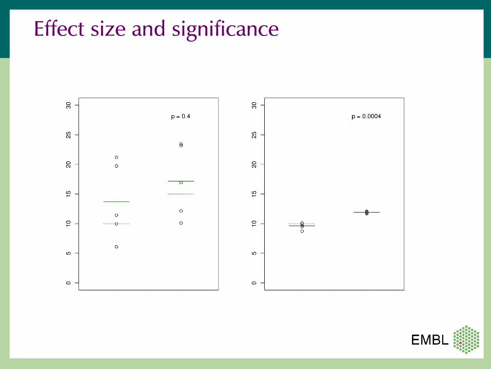
Effect size and significance

Variance calculated from comparing two replicates

Poisson v = μ Poisson + constant CV v = μ + α μ2

Poisson + local regression v = μ + f(μ2)

Variance depends strongly on the mean

Technical and biological replicates

RNA-Seq of yeast [Nagalakshmi et al, 2008]

biological replicatestechnical replicates

Poisson (I)

• The Poisson distribution turns up whenever things are counted

• Example: A short, light rain shower with r drops/m2. What is the probability to find k drops on a paving stone of size 1 m2?

Poisson (II)

For Poisson-distributed data, the variance is equal to the mean.

Hence, no need to estimate the variance according to several authors: Marioni et al. (2008), Wang et al. (2010), Bloom et al. (2009), Kasowski et al. (2010), Bullard et al. (2010)

• Really?Is HTS count data Poisson-distributed?

To sort this out, we have to distinguish two sources of noise.

Shot noise

• Consider this situation:• Several flow cell lanes are filled with aliquots of the same

prepared library. • The concentration of a certain transcript species is exactly the

same in each lane. • We get the same total number of reads from each lane.

• For each lane, count how often you see a read from the transcript. Will the count all be the same?

Shot noise

• Consider this situation:• Several flow cell lanes are filled with aliquots of the same

prepared library. • The concentration of a certain transcript species is exactly the

same in each lane. • We get the same total number of reads from each lane.

• For each lane, count how often you see a read from the transcript. Will the count all be the same?

• Of course not. Even for equal concentration, the counts will vary. This theoretically unavoidable noise is called shot noise.

Shot noise

• Shot noise: The variance in counts that persists even if everything is exactly equal. (Same as the evenly falling rain on the paving stones.)

• Stochastics tells us that shot noise follows a Poisson distribution.

• The standard deviation of shot noise can be calculated: it is equal to the square root of the average count.

Sample noise

Now consider• Several lanes contain samples from biological

replicates.• The concentration of a given transcript varies

around a mean value with a certain standard deviation.

• This standard deviation cannot be calculated, it has to be estimated from the data.

Technical and biological replicates

Nagalakshmi et al. (2008) have found that• counts for the same gene from different technical

replicates have a variance equal to the mean (Poisson).

• counts for the same gene from different biological replicates have a variance exceeding the mean (overdispersion).

Marioni et al. (2008) have looked confirmed the first fact (and confused everybody by ignoring the second fact).

Technical and biological replicates

RNA-Seq of yeast [Nagalakshmi et al, 2008]

biological replicatestechnical replicatesPoisson noise

Summary: Noise

We distinguish:• Shot noise

• unavoidable, appears even with perfect replication

• dominant noise for weakly expressed genes

• Technical noise • from sample preparation and sequencing• negligible (if all goes well)

• Biological noise• unaccounted-for differenced between samples• Dominant noise for strongly expressed genes

can becom

p utedneeds to be estim

atedfrom

t he da ta

Which null hypothesis?

In a statistical test, we attempt to reject a null hypothesis. Given two samples with different experimental conditions, which null hypothesis covers the question of biological interest?• The concentration of transcripts from gene i is

equal in the two samples.➔ shot noise is all we need to know

• The difference of the concentrations is of a magnitude as is expected between replicate samples.➔ Estimate of biological variability needed

The negative-binomial distribution

A commonly used generalization of the Poisson distribution with two parameters

The NB distribution from a hierarchical model

Biological sample with mean and µvariance v

Poisson distribution with mean q and variance q.

Negative binomial with mean µ andvariance q+v.

Testing: Null hypothesis

Model:The count for a given gene in sample j come from negative binomial distributions with the mean sj μρ and variance sj μρ + sj

2 v(μρ).

Null hypothesis:The experimental condition r has no influence on the expression of the gene under consideration:

μρ1 = μρ2

sj relative size of library jμρ mean value for condition ρv(μρ) fitted variance for mean μρ

Model fitting

• Estimate the variance from replicates• Fit a line to get the variance-mean dependence v(μ)

(local regression for a gamma-family generalized linear model, extra math needed to handle differing library sizes)

Testing for differential expression

• For each of two conditions, add the count from all replicates, and consider these sums KiA and KiB as NB-distributed with moments as estimated and fitted.

• Then, we calculate the probability of observing the actual sums or more extreme ones, conditioned on the sum being kiA+kiA, to get a p value.

(similar to the test used in Robinson and Smyth's edgeR)

Differential expression

RNA-Seq data: overexpression of two different genes in flies [data: Furlong group]

Type-I error control

Comparison of replicates:

no differential expression,

expect uniform p values

low high all

DES

eqed

geR

Pois

son

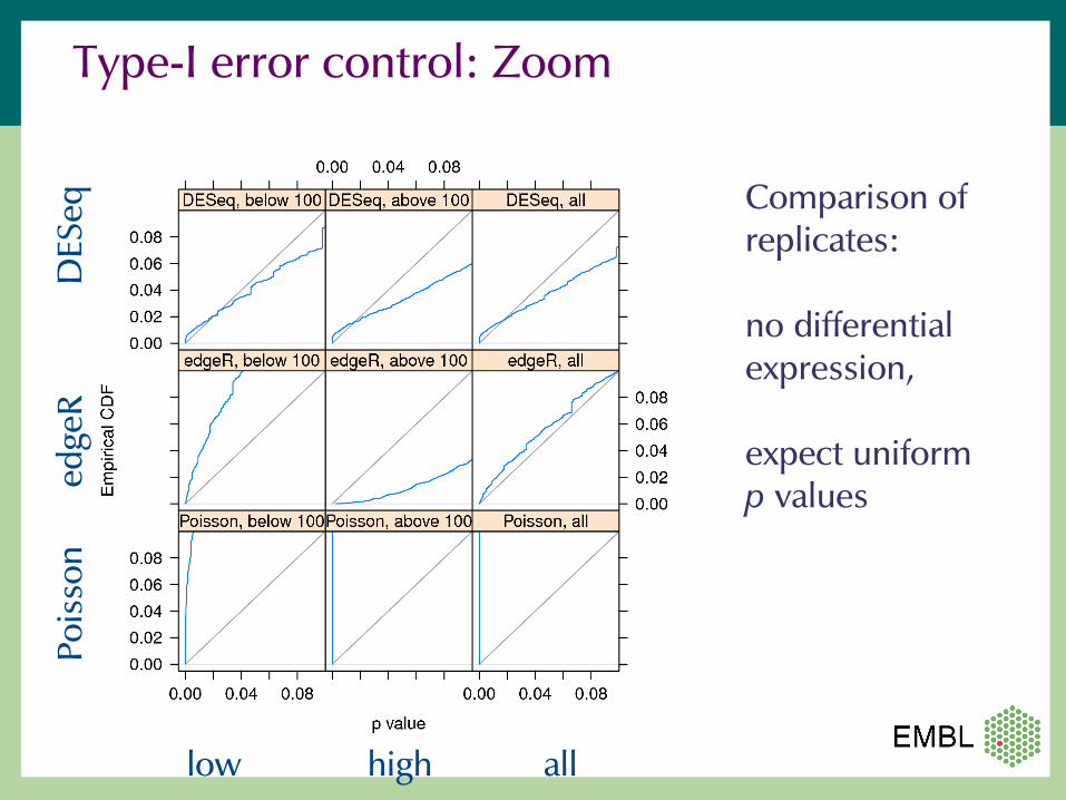
Type-I error control: Zoom

Comparison of replicates:

no differential expression,

expect uniform p values

low high all

DES

eqed

geR

Pois

son

Distribution of hits along the dynamic range

all genesdifferentially expressed according to DESeq differentially expressed according to edgeR

Two noise ranges

dominating noise How to improve power?shot noise (Poisson) deeper samplingbiological noise more biological replicates

Working without replicates

One can infer the variance from a comparison of different conditions.• The variance will be overestimated, maybe

drastically.• The power is smaller, maybe much smaller.

Still, this is the best one can do without replicates.

Variance-stabilizing transformation

The estimated variance-mean dependence allows to derive a transformation that renders the count data approximately homoskledastic.

This is useful, e.g., as input for the dist function.

[Tag-Seq of neural stem cell tissue cultures,Bertone Group]

Further use cases

Similar count data appears in• comparative ChiP-Seq• barcode sequencing• ...and can be analysed with DESeq as well.

Alternative splicing

• So far, we counted reads in genes.• To study alternative splicing, reads have to be

assigned to transcripts.• This introduces ambiguity, which adds uncertainty.• Current tools (e.g., cufflinks) allow to quantify this

uncertainty.• However: To assess the significance of differences

to isoform ratios between conditions, the assignment uncertainty has to be combined with the noise estimates.

• This is not yet possible with existing tools.

Coming soon: GLMs for DESeq

• Until now, DESeq only supported simple comparisons.

• There are many use cases requiring more general models.

• Implementation of generalized linear models (GLMs) for DESeq now ready for use.

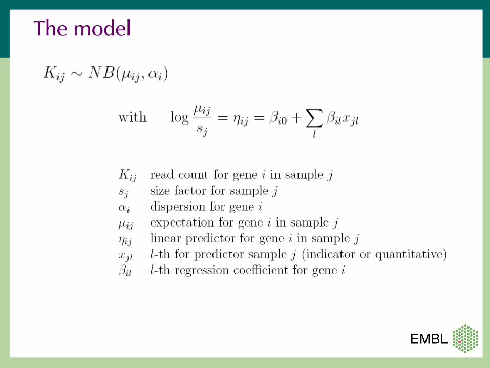
The model

The model

• This is a generalized linear model:• Link function: log link, with sample-dependent size factors• Family: negative binomial with known dispersion

• The dispersion is estimated from the fitted variance-mean relation, reading off at the sample average:

• The negative binomial is in the exponential family if the dispersion is given.

DESeq with GLMs: Applications

• Factorial designs with interactions• Paired samples• Regression of expression on genotype, etc.• Alternative splicing

• Count for each exon, then fit a model for each gene, and test the interaction between exon and experimental condition.

• Methylation (HELP)• ChIP-Seq: ChIP vs input crossed with condition

Conclusions

• Proper estimation of variance between biological replicates is vital. Using Poisson variance is incorrect.

• Estimating variance-mean dependence with local regression works well for this purpose.

• The negative-binomial model allows for a powerful test for differential expression

• Preprint on Nature Preecedings:“Differential expression analysis for sequence count data”

• Software (DESeq) available from Bioconductor and EMBL web site.

*

• Co-author: Wolfgang Huber

• Funding: European Union (Marie Curie Research and Training Network “Chromatin Plasticity”) and EMBL

Google forDESeq

Negative-binomial model (I)

• Suppose, we have m replicates of a given condition, and obtain counts for n genes.

• The concentration of gene i in replicate j is a random variable Qij, which is i.i.d. for j=1,...,m with mean qi0 and variance σi².

• Let Kij be the count value for gene i in replicate j. Its expectation value is sjμi with size factor sj.

• Given Qij=qij, the sequencing is a Poisson process

and hence: Kij Pois( sjqij ).

Negative-binomial model (II)

• If Qij has mean μi and variance σi², what is the the

marginal (“mixing”) distribution of Kij Pois( sjqij ) ?

• If one assumes Qij to be gamma-distributed, the answer is:

• Kij follows a negative binomial (NB) distribution with mean sjqi0 and variance sjqi0 + sjσi².

Model fitting

• Estimate relative library sizes sj.

• Within a set of replicates, calculate for each gene sample mean and sample variance of kij/sj.

• To get an unbiased estimate of σi², subtract an “average shot-noise” of

• Fit a line through the graph of mean and variance estimates (with a gamma-family local regression).

Model:Kij follows a negative binomial (NB) distribution with mean sjqi0 and variance sjqi0 + sjσi².

Diagnostic plot for variance fit

Variance residuals distribution

per-gene sample variance / fitted variance

dens

ity