differential calculus for functions from … bound... · differential calculus for functions from...

R 877 Philips Res. Repts 29, 560-586, 1974

DIFFERENTIAL CALCULUS FOR FUNCTIONSFROM (GF(p))1I INTO GF(p)

by A. THAYSE

Abstract

The differential calculus for functions mapping the field of integersmodulo p into itself encompasses and generalizes the concepts introducedby the author in several previous papers on Boolean differential calculus.In this paper the attempt is made to subsume a set of results in a singleconsistent theory very close to the classical differential calculus. It ispointed out that the use of appropriate computational formulas leads tofairly simple solutions for various kinds of problems such as, e.g., thetesting of p-ary networks whose realization is based on Taylor expan-sions and the computation of Stirling numbers.

1. Introduction

It is classical to say that the Boolean differential calculus has been introducedin a paper by Akers 12). Akers defined the concept of partial derivative of aBoolean function and showed it to be a measure of the invariance of thefunction on an edge of the 2n cube which is the domain of definition of thefunction. Further he proved that this concept is closely related to the conceptof partial derivative and he obtainedimportant theorems analogous to McLaurinand Taylor expansions, thus giving a basis to Boolean differential calculus. Thistheory has been extended in three papers by the present author 15-17) intro-ducing, among other things, the concepts of Boolean differential, of meet andof join derivatives, and deriving the relations between these concepts and theclassical notion of prime implicant of a Boolean function. A theory of finitedifferences for multivalued functions has been introduced in refs 1, 2 and 4,one of them showing that this theory reduces to Boolean differential calculusfor binary functions. The main purpose of this paper is to introduce and todevelop a differential calculus for functions, mapping the field of integersmodulo p into itself and then show that this theory again reduces to Booleandifferential calculus for binary functions. A first self-evident conclusion is thusthat the Boolean differential calculus coincides with the Boolean calculus ofdifferences. Consequently the Boolean derivative and the Boolean differenceconstitute the same concept, the Boolean differential and the Boolean incrementlikewise.In the present paper, discrete function will be a nomenclature applied exclu-

sively to functions from (GF(p»" into GF(p). The notion of partial derivativeof a discrete function, already briefly introduced in ref. 2, is recalled in sec. 2.2,

DIFFERENTIAL CALCULUS FOR FUNCTIONS FROM (GF(p»n INTO GF(p) 561

and its main properties are studied. The notion of total differential is introducedin sec. 2.3; important properties of this differential are also derived. Let us,among other things, point out that the differentials are related to the incrementsof a discrete function (defined in refs 2 and 4) through the intermediate of theStirling numbers evaluated in the field of integers modulo p. This generalizes tofinite fields some well-known relations between derivatives and differences innumerical analysis.In sec. 2.4 explicit formulas are derived for the computation of the derivatives

and ofthe differences from the function truth vector. More precisely, it is knownthat the Kronecker factorization of a transformation matrix is equivalent to theexistence of an order-lowering algorithm that replaces a problem in n variablesby two problems in n - I variables. This idea is then applied to the evalua-tion of the derivatives and of the differences.

Sections 2.5 and 2.6 study the usefulness of the representation of a discretefunction by means of easily constructed p-ary vectors having (p (p - I) + l)"components and called extended truth vectors. It is shown that, starting fromthe extended truth vectors, it is possible to compute the Taylor expansions andthe Newton expansions with a [cp (P-I) + 1)/p2]n saving in complexity com-pared with algorithms computing each of the derivatives and each of the dif-ferences in an extensive way. The contents of secs 2.5 and 2.6 are a straight-forward generalization of a computation method for Boolean functions due toBioul and Davio 10.16). Section 2.7 briefly considers some special features suchas, e.g., the derivatives of functions of functions and some related problems.Section 3 is devoted to some possible applications of the differential calculus

quoted above. First of all let us point out that several authors 8.18.19) haveindicated the advantages in terms of increased speed and capacity, together withdecreased cost and complexity, of employing multivalued switching devices inplace of conventional binary elements. These advantages seem to be especiallyrelevant to applications in digital computers and automatic control. Theauthoritative work of Green 18.20) on nonllnear ternary feedback shift registersdeserves special mention.

Our intention in sec. 3.1 is to present a new application related to multivaluedswitching devices. It is well known from Reddy's work 21) that any realizationfor an arbitrary Boolean function, using AND and exclusive-OR gates, basedon Taylor expansions, has many desirable properties so long as its tests areconsidered. More precisely, Reddy shows that if the primary leads are fault-free,then there is a realization for an arbitrary n-variable logic function that requiresa fault-detection test set with only n + 4 tests and this test set is independentof the function being realized. The first aim of sec. 3.1 is to show that therealization of a multivalued network based on one of its Taylor expansions,also presents attractive properties from a diagnostic point of view. First of all,the stuck-at-fault model is generalized for p-valued functions. It is then shown

562 A.THAYSE

that testing the network requires at most p + 1+ n (p - 1) tests.In sec. 3.2 we present an application which is closely connected to numerical

analysis. We show that the formulas, based on the discrete differential cal-culus developed here, allow us to obtain attractive closed expressions for com-puting the Stirling numbers in the field of integers modulo p. The Chineseremainder theorem is then used to evaluate the real value of these Stirlingnumbers.The notations in this paper are those used in refs 1 and 2. They will not be

recalled here.

2. Derivation operators and Taylor expansions for functions from (GF(p»n intoGF(p)

2.1. Functionsfrom (GF(p»n into GF(p)

Let us first recall the definition of a discrete function (see refs 1 and 2). Let5 be the direct product of n finite sets St:

S=Sn-1XSn_2X."XSO= X 5"t=n-1.0

and let L= {a, 1, ... , r - I}. We call discrete function any mapping

F:S-L.

The function F: S_ L may be denoted asf(xn_1"'" Xl' Xo), the variable XI

taking its value in the set SI'We shall now choose an enumeration order of the points of the domains 5;

let us first define (for each subscript i) a one-to-one mapping of SI into the setof integers {a, 1, ... , mi-I}. The lexicographical order is then chosen forthe enumeration of the points in the domain. With this convention we are ableto define any discrete function by the corresponding set of values {J;},j = {jn- h jn-2' ... , jo}, i.= 0, 1, ... , mi - 1, V i; J; EL Vj. We shall finallychoose an enumeration order of the points of the domain L by defining a one-to-one mapping of L on to the set of integers {a, 1, ... , r - I}.The set of discrete functions may be studied by assigning to it different

mathematical structures. Two previous parts of this work 1.2) were devotedto the study of the lattice and of the ring structures of discrete functions ..Thepurpose of this paper will be to study more thoroughly the important particularcase of discrete functions for which

So = 51 = ... = Sn-l = L= {a, 1, ... ,p-l},

p being a prime, i.e. functions from (GF(p»n into GF(p).It is well known that a field with l! elements, provided p is prime, can be

formed by taking the integers modulo p, so that the elements can be labelled

àkOf = àko

(~( ... (àkq-1f) ... ))

àxo àxo àXl àXq_l

with ko = {ko, kt> ... , kq-l} and Xo = {xo, Xl' ... , xq-d. Conventionallyit is assumed that ào_t;àxo = j.It can easily be shown that the operator à/àx, has the characteristics of a

classical derivation operator; the following properties apply (see ref. 1):

(3)


as consecutive integers 0, 1, ... , p - 1. The basic operations are called sum(in the field) written as Et> or :E, and product in (the field) symbolized by ITor simply by juxtaposition of the operands, The field exponentiation x" willbe used with its usual meaning, that is,

xe=x X X ... X~

e times

2.2. Derivatives and Tay/or expansions

Given a functionj(xn_l, Xn-2, ... , xo) =f(x) from (GF(p))n into GF(p),the derivatives of fex) were defined in ref. 2 as follows:

Definition 1

(a) Simple derivativesp-l

'Of =_(~f(X,E9j~-f(X)).'OX, ~ ]

)=1

(1)

(b) Multiple derivatives

'Ok'.!_ à (àkl-lf)--- ---,'Ox, 'Ox, 'Ox,

(2)

àc-=0,'Ox,

à(clfl E9c2f2) àfl 'öf2------ = cI-E9 C2-'

'Ox, 'Ox, 'Ox,

'ti CE GF(p), (4)

(5)

à ('Of) à ('Of)'Ox, 'Ox) = 'Ox) 'Ox,'àxm_=mxm-l'Ox '

(6)

m :::;;;p-1. (7)

Besides these computational properties, let us also point out that f (x) is de-generate with respect to x, if, and only if, àf/àx, = 0. Indeed, in view of(4)-(7) it is clear that the derivative of a function applying GF(p) into itself

(9)

564 A.THAYSE

is given by formal derivation of the polynomial which represents it. Moreover,it is well known (see e.g. ref. 3) that any function on GF(p) may be expandedaccording to the following polynomial expression:

p-1

:E aJx/,J=O

where the aJ are independent of Xl' Since there is a one-to-one correspondencebetween these polynomials and the set of functions on GF(p), a polynomialhaving its aJ 'tij > ° identically zero corresponds to a nul derivative uf/uxland consequently the primitive function reduces to ao, that is, a function inde-pendent of Xl' In view of the above properties it is clear that Uf/UXI shares mostof its properties with the classical notion of derivative.The two following theorems, proved in ref. 1, show the importance of the

concept of derivative as a theoretical tool by giving the relations of thesederivatives with the coefficients of the polynomial expansions of a functionf(x).

Theorem 1

Any function f (x) may be expanded asn-1

E(UCj(X)) [0X/I]f(x)= -- - ,'Ox x=o el!

(8)

e 1=0

Theorem 1 is called the McLaurin expansion of the function f (x), since itinvolves only the values of the derivatives at x = O. The theorem 2 will anal-ogously be called the Taylor expansion of the function.

Theorem 2

For any functionf(x)n-1

e 1=0

e = eo, el' , en-I,h= ho, hl, , hn-1>

°~ el ~p-1,hl E {a, 1, ... , p - I} 'ti i.

Theorem 2 applied to the function f(x $ h) leads to the following relation:n-l

E(UCj(X)) [OX/I]f(x EB h) = -- - .'Ox xee h el!

(10)

e 1=0

E è:>Cj(x) [0h{']f(xEBh)-/(x)= -- - ,öx et!

(11)


The last equation constitutes an alternative statement of theorem 2. Notefurther that an interchange of the roles played in (10) by x and h allows us towrite:

p-l

e t=O

e =1= 0, 0, ... , 0.

This last expansion will be used further on in this text.

2.3. The total difference

The increments t!..,! of a discrete function were defined in refs 2 and 4. Theincrements play a key role in the discrete difference calculus for two basicreasons. First of all they are a parametrical form of the set of difference opera-tors (namely the partial difference and the sensivitity) for discrete functions andconstitute a compact way of representing and of evaluating these operators. Onthe other hand they are useful tools for computing the difference operators ofdiscrete functions. In this section one will define and study the total differen-tials d'! of a function! It will be seen that the total differentials play the samerole with respect to the derivatives as the increments do with respect to thedifferences of!Let us first briefly recall some of the definitions and properties of the incre-

ments. The first increment Sf of f is the function:

t!..f =I(x EBLh) - I(x)n-l

(12)

e j=O

In view of relation (12), it appears that the increment Sf of a discrete func-tion f is a parametrie form of the set of all the sensitivities associated with f,that is,

n-l

e j=O

(13)

The qth increment was defined iteratively, that is,

(14)

566 A.THAYSE

From (13) and (14) one then deduces:

(15)

Let us also observe that tl.'Ijcannot lead to the computation of operators ofthe form

~: (~: (. .. (Sk~~!f) .. .)).

The total differentials d,! off (x) will now be defined through the intermediateof the increments Mf

Definition 2

(a) Simple differentialp-l

(~)df=- E htl.'J,

'.h=!

(16)

(b) Multiple differential

(17)

Let S,(k) and S,(k) be the Stirling numbers of the first and of the second kind,respectively. The following theorem relates in closed form the increments andthe total differentials.

Theorem 3

(a) k~p-l; (18)

(b)

'=k

p-l

£ S (k)k'

dkf = -'--' tl.'J,i! '

k ~p-1. (19)

I=k

Proof

From the theorems 3.11 and 3.12 of ref. 2, one immediately deduces:

1=1 h=O

p-1 p-1(h)

dkf= E[-k!(E ~k)~11 (21)


p-1 p-1

(20)

1=1 h=1

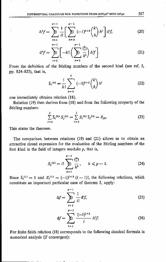
From the definition of the Stirling numbers of the second kind (see ref. 5,pp. 824-825), that is,

k

S,Ck) = ~!I (_1)1I+k (~) h'

1,=0

(22)

one immediately obtains relation (18).Relation (19) then derives from (18) and from the following property of the

Stirling numbers:J J" 5 (k) S (I) - " S (k) 5 (I) _ .s:L..., I J - L..., I J - uIk» (23)I=k I=k

This states the theorem.

The comparison between relations (19) and (21) allows us to obtain anattractive closed expression for the evaluation of the Stirling numbers of thefirst kind in the field of integers modulo p, that is,

p-1

(1)S(k)=i! ~ -I ~hk'

h=1

k~p-1. (24)

Since 5,(1) = 1 and S,(1) = (_1)'+1 (i- I)!, the following relations, whichconstitute an important particular case of theorem 3, apply:

p-1

~f= ~ 2_d~~i! '

(25)

1=1

p-1

~ (_1)'+1df= ~ ~'f. (26)

1=1

For finite fields relation (18) corresponds to the following classical formula innumerical analysis (if convergent):

568 A.THAYSB

0()

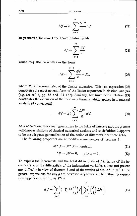
IS<k)D.y= k! -'_d1..,

I.(27)

I=k

In particular, for k = 1 the above relation yields0()

Id,!D.f= - .,

I.(28)

1=1

which mayalso be written in the formn-1

Id,!D.f= -+Rm.,

l.

, (29)

1=1

where R; is the remainder of the Taylor expansion. This last expression (29)constitutes the most general form of the Taylor expansion in classical analysis(e.g. see ref. 6, pp. 85 and 134-137). Similarly, for finite fields relation (19)constitutes the extension of the following formula which applies in numericalanalysis (if convergent):

0()

(30)

I=k

As a conclusion, theorem 3 generalizes to the fields of integers modulo p somewell-known relations of classical numerical analysis and so definition 2 appearsto be the adequate generalization of the notion of differential for these fields.

The following properties are immediate consequences of theorem 3:

D.P-1j= dP-1f= constant, (31)

(32)D.'Ij= dilj= 0, q>p-l.

To express the increments and the total differentials of f in terms of the in-crements or of the differentials of the independent variables x does not presentany difficulty in view of theorem 3 and of the results of sec. 2.5 in ref. 1; thegeneral expressions for any p are however very tedious. The following expres-sion applies (see ref. 1, eq. (22»:

J

(33)

J=O 1=0

(34)


In view of (19) and (33) one then obtains the expression of the kth differentialin terms of the differentials of its. independent variables, that is,

I,J r,l

where d'x = {drxo, drxt, ... , drxn_1}'.The above formulas yield for p = 2 and 3 respectively:

p=2:df = 6.f =f(x Ei:)Lh) Et> f(x)

=f(x Ei:)dx) Et>f(x);

p= 3:6.f = f (x Ei:) Lh) Ei:) 2f (x)

= f(x Ei:) dx Et> 2 d2x) Ei:) 2f(x),df=f(x Ei:) 21l.x Ei:)d2x) Et> 2f(x Ei:)dx)

= f(x Ei:) 2 dx Ei:)2 d2x) Et> 2f(x Ei:)dx Ei:) 2 d2x),d2f= 6.2f=f(x Ei:) 21l.x Ei:)d2x) Et>f(x Ei:)dx) Ei:)f(x)

= f(x Ei:) 2 dx Ei:)2 d2x) Et> f(x Ei:)dx Ei:) 2 d2x) Ei:)f(x).

From (21), one successively deduces:

1=1 11=1(in view of (21))

(in view of (15))

1=1 11=1

(in view of theorem 3.11 of ref. I).

The differentials are thus also, among other things, parametrical forms of thederivatives.

As a conclusion of this section, the concept of total differential (in the fieldGF(p)), which may be considered as an extension of the classical differential,is introduced. The purpose of the following sections will be to use the conceptsof derivatives and of differentials in order to derive various properties of func-tions from (GF(p))n into GF(p).

570 A.THAYSE

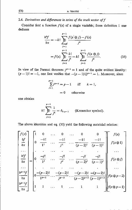
2.4. Derivatives and differences in terms of the truth vector off

Consider first a function f(x) of a single variable; from definition 1 onededuces

p-1'è)"f = -kl ~ f(x' $ j) - f(x)öx .l:..J jk

J=lp-1 p-1

k! Ef(X$j)=f(x) --kl .

f rJ= 1 J=1

(35)

In view of the Fermat theorem: jP-1 = 1 and of the quite evident identity:(p -I)! = -1, one first verifies that -cp _1)!/jP-1 = 1. Moreover, since

iff k= 1,J=1

= 0 otherwise

one obtainsp-1

k! ~ 2_ = t5kP-1.l:..Jjk(Kronecker symbol) .

J=1

The above identities and eq. (35) yield the following matricial relation:

f(x) 1 0 0 0 0 f(x)'è)f -l! -l! -l! -l!

0 f(x (f) 1)'è)x 11 F (p _ 2)1 (p _ 1)1

'è)1j'0

-j! -j! -j! -j!f(x (f)j)

'è)x IJ jJ (p-2)1 (p -1)J

'è)P-2f -(p-2)! -(P-2)! -(p-2)! -cP -2)!f(x(f)p-2)o ...

'è)x p-2 jP-2 (p - 2)p-2 (p _1)P-2

'è)P-1f1 1 1 1 1 f(x(f)p-l)

'è)x


which, written more concisely, gives

SflSx = B aflax (36)

with

SflSx = [f(x), 'öfl'öx, 'ö2f1'öx, ... , 'öP-1f1'öx]t,

oflax = [f(x),J(x E9 1),J(x E9 2), .•. ,J(x EBP _1)]t,

B = [bIJ]= [-(i-l)!fU-l)'-1] iff i,j ~ 2= ~1 J iff i = 1, j ~ 1= ~P I iff j = 0, i ~ 2.

The inverse transformation is written

ofiox = B-1 SflSx. (37)

The element bIJ-1 of B-1 immediately derives from the relation (11), that is

B-1 = [bIJ-1] = [(i-l)J-1f(j-l)!].

Consider the vector

AflAx = [f(x), /:ifl/:ix, /:i2f1/:ix, ... , /:ip-1f16.X]t.

Theorem 2.1 of ref. 1 allows us to write

AflAx = A ofiax,

ofkxx = A -1 AfI Ax,

(38)

(39)

with

A = [a,J = [(_I)I+J C=~)J.A-1 = [aIJ-1] = [c=~)1

Similarly, theorem 3 allows us to write

AflAx = S SflSx,

SflSx = S-1 AflAx,

(40)

(41)

with'

S= [sIJ] = [(i -I)! SJ_1(1-1)f(j -I)!],

S-1 = [S'J-1] = [(i-I)! SJ_1(1-1)f(j-I)!].

Relations (36)-(41) constitute a complete characterization of the transforma-tions between the systems of vectors aflax, SflSx and Affllx.

572 A.THAYSE

The extension of the above results to multivariable functions can now easilybe performed by use of the Kronecker product.The (l xpn) matrices af/ax, Sf/Sx and 1lf//1x (with x = Xo, Xl> ••• , xn-l)

are defined as follows:

°a/fax = [ ® afaxil f (x),

t=n-lo

Sf/Sx = [ ® SfSxt]f(x),t=n-l

°/1f//1x = [ ® /1f/1xt]f(x).

t=n-l

The nth Kronecker power of a matrix X is denoted by X".Thanks to the properties ofthe Kronecker product and to the results obtained

above we can now state the following theorem.

Theorem 4

(a) Sf/Sx = B" af/ax, (42)

(b) af/ax = (B-l)n Sf/Sx, (43)

(c) /1f//1x = An af/ax, (44)

(d) af/ax = (A-l)n /1f//1x, (45)

(e) /1/f/1x = S" Sf/Sx, (46)

(f) S/fSx = (S-l)n /1f//1x. (47)

The truth vector [f.,] of the discrete functionf(x) will be defined as

[f.] = [af/ax]x=o·

The truth vectors of the derivatives and of the differences may then easily bededuced from theorem 4.

Consider first a function of a single variable. From relation (36) one deduces

(oiJ) = [0 j!... 1!... -j! -j! ] [Ie]ox x=O IJ i' (p - 2)J (p - I)J

= bj+l[fc] (bJ+l is the (j + l)th row of B),

(oJf) = [-j! 0 j!... c: -j! ] [Ie]ox x= 1 (p - I)J 1J j1 (p - 2)1

= \l bJ+l [Ie],


where \l bHl clearly means a vector obtained by shifting from one columneach element of bJ+l to the right. The vector \lk bHl will be defined as

The jth derivative of f is then given by the matricial relation

'öJf/'öx = [bJ+l' \l bJ+l' ... , \lp-2 bJ+l, \lP-l bHl]t [f.]

= BJ Lt;,]·Let aHl be the (j+ l)th row of the matrix A; using similar arguments asabove one easily deduces that

t::..Jf/tu = [aJ+!> \l aJ+l' ... , \lp-2 aJ+l' \lp-l aHl]t [f.]

= AJ [Ic]·

Thanks to the properties of the Kronecker product and to the results obtainedabove we are able to deduce the following theorem:

Theorem 5

'ö1J 'öJoh ...Jn-lf 0

(a) e BJI [Ie], o <i. ~p-l; (48)'öx 'öXOXl ... Xn-l I=n-l

!lIJ !lJoh ...Jn-lf 0

(b) - e Ail [Ie], o ~jl ~p-l. (49)!lx !lXOXl ... Xn-l I=n-l

The result of theorem 5 constitutes a straightforward generalization of a prop-erty which was quoted for Boolean functions in ref. 9.It may be useful to note that polynomial expansions of functions from

(GF(p))n into GF(p) are well known, and their study goes back to Bernstein 11).Since this early paper several authors have used these expansions, so thatmatricial forms similar to B and B-1 may, e.g., be found in refs 3, 7 and 8.

2.5. Taylor expansions of discrete functions and of their derivatives

The existence of Taylor expansions of Boolean functions is known from thework of Akers 12). Since then several authors have raised the problem offindingan optimal Taylor expansion, i.e. an expansion having a minimum weight(number of summed terms). Generally, the available solutions all amount tothe generation of 4n coefficients since there are 2n derivatives which must becomputed at 2n vertices of the n-cube. In a recent paper 10), Bioul and Davioshowed that a closer observation of the Taylor expansions leads to the con-clusion that there are only 3n different coefficients instead of 4n• Their paperdescribes a direct way of generating these 3n coefficients and, from that point

574 A.THAYSE

on, computing the Taylor expansions with a corresponding (3/4)" saving incomplexity.

This section contains a straightforward generalization of the Bioul-Daviomethod to discrete functions from (GF(p))" into GF(p). Since for these func-tions there are p" derivatives which must be evaluated at p" vertices, the directcomputation leads to the generation of »" coefficients. It is shown in thissection (by using arguments similar to those developed by Bioul-Davio) thatthere are only (p2 - P + 1)" different coefficients instead of p2". This sectiondescribes a direct way of generating these coefficients and, from that point on,computing the' Taylor expansions with a corresponding (1 - lip + 1/p2)"saving in complexity.

Let [fe] be the truth vector ofI (x). The extended truth vector (with respectto the Taylor expansions) of I (x), denoted by <PT is defined by

(50)

where MT" is the nth Kronecker power of the [cp (p -1) + 1)X (P)] matrix:

BoBi

Bp_2

1, 1, ... , 1

Since the matrices BJ are p <» matrices, the extended truth vector <PT has thus(p (p -1) + I? components.The derivative

()p-l.p-l .... p-l.kmkm+ 1·.. kO-1f

with k, < p - 1 'V i depends only on the n - m variables Xm, Xm+ 10 ••• , X"-l'

There are

derivatives of this kind, each of which must be evaluated at (p _1)"-m dif-ferent vertices. Hence, there are

I"

m=O

vertices where the derivatives are to be evaluated, i.e. also (p (p - 1)+ 1)"Taylor expansions of derivatives of f As usual, a computation saving is

DIFFERENTIAL CALCULUS FOR FUNCTIONS FROM (GF(p))" INTO GF(p) 575

achieved by the choice of a suitable enumeration order of these expansions.For this purpose we introduce the following notations. First let I(x) be afunction of a single variable x. Then the symbol T/J denotes the Taylor ex-pansion at the vertex h of the jth derivative of J (0 ~ j ~ p - 1); the nota-tion [1//] will denote the matrix of operators:

Since ()il-1f/()X does not depend on X, the notation Thp-1 has been substitutedby Tp-1 in the above matrix. Next, for a function J(x) of n variables, thematrix [Tbl] is defined as the formal Kronecker product

where the product of two operators is achieved by concatenating the indices hland j.,

Consider the following matrix K, defined for p = 3:

1 0 0(XI- 0)1

0 0(XI-O)Z-

1! 2!

0 1 0 0(XI-I)1

0(XI -1)2

1! 2!

0 0 1 0 0(xl-2)1 (xl-2)Z

1! 2!

0 0 0 1 0 0(XI-O)1

1!

0 0 0 0 1 0(XI-1)1

1!

0 0 0 0 0 1(xl-2)1

1!

0 0 0 0 0 0 1

576 A.THAYSB

The expression of the matrix KI for any p easily derives from the above example.Theorem 6 relates the (p (p -1) + 1)"Taylor expansions of f and of itsderivatives to the extended truth vector.

Theorem 6

The (p (p - 1) + 1)" Taylor expansions of the derivatives of the functionf (x) are given by

[TH(x)] = C=~_!KI)q>T' .

The proof of theorem 6 is exactly the same as that of the corresponding propertyof Boolean functions given by Bioul-Davio !O) and need not be given here.Now consider the restrietion of (51) to O-derivatives; in this case the matrix KI

reduces to a matrix HI which is defined e.g. for p = 3 as follows:

(51)

1 0 0(XI-O)!

0 0(XI-O)2

1! 2!

0 1 0 0(xI-I)!

0(xl-l)2

1! 2!

(XI- 2)! (XI- 2)2

0 0 1 0 0 1! 2!

Corollary

The p" Taylor expansions of the functionf(x) are given by

[ThOf(x)] = (=~_!HI) q>T'

Let us now define the matrices KI*, HI* and q>T* which are nothing but thematrices Kb HI and q>Twhere the non-zero entries have respectively beensubstituted by 1. The weights of the Taylor expansions may then be evaluatedby means of the following theorem which is again a straightforward generall-zation of a theorem by Bioul-Davio for Boolean functions.

(52)

Theorem 7

The weights of the (p (p - 1)+ 1)" Taylor expansions of the derivatives ofthe function f(x) are given by

[WTblf(x)] = (=~_!KI*) X q>T* (53)

where X means the real matrix product.

DIFFERENTIAL CALCULUS FOR FUNCTIONS FROM (GF(p»" INTO GF(p) 577

Corollary

The weights of the p" Taylor expansions of the function f(x) are given by

(54)

It turns out from all the above theorems and corollaries that the extendedtruth vector CPT contains, in relatively condensed form, all the informationnecessary to arrive simply at the Taylor expansions of a discrete function andof its derivatives.

2.6. Newton expansions of discrete functions and their differences

It is clear that all that was said in sec. 2.5 concerning the Taylor expansionsof the derivatives of f could be transposed to the Newton expansions of thedifferences off Some results are briefly quoted in this section; the statementswould be the same as those of sec. 2.6.There are (p (p -1) + 1)"Newton expansions of differences of f If f(x)

is a function of a single variable x, the symbol NhlJ denotes the Newton ex-pansion at the vertex h of the jth difference off; the notation NhJ will denotethe matrix of operators:

N p-2p-1Np-1

For a function f(x) of n variables, the matrix [Nbl] is defined as the formalKronecker product

o

The extended truth vector (with respect to the Newton expansions) of f(x),denoted by CPN is defined by

CPN =MN" [fel

where MN" is the nth Kroneeket power of the [cp (p - 1) + 1)X (P)] matrix

578 A.THAYSE

AoAl

MN= (55)Ap_2

1, 1, ... , 1

Consider the following matrix El defined for p = 3:

1 o 0 (XI~O) 0 0 (XI~O)I

0 1 0 0 (XI~ 1) 0 (XI~ 1)o 0 1 0 0 (XI~2) (XI~2)

000 1 0 0 (XI~O)

000 0 1 0 (XI~ 1)

0 0 0 0 0 1 (XI~2)0 0 0 0 0 0 1

The formulation of the matrix El for any p easily derives from the aboveexample.

Theorem 8The (p (p - 1)+ 1)" Newton expansions of the differences of the func-

tion I (x) are given by

[Nb' I (x)] = C=~_IEI ) ({>N'

Now consider the restrietion of (56) to O-differences. In this case the matrix Elreduces to a matrix FI which is the matrix of the p first rows of E"

(56)

Corollary

The p" Newton expansions of the function I(x) are given by

[NbOI(x)] = C=~-/I) ({>N' (57)


Let us now define the matrices E,*, F,* and <{>N*as the matrices Eh F, and <{>Nwhere the non-zero entries have respectively been substituted by 1.

Theorem 9

The weights of the (p (p - 1) + l)" Newton expansions of the differencesof the functionf(x) are given by

[W Nbl f(x)] = C=~_lEI* )X<{>N*. (58)

Corollary

The weights of the pn Newton expansions of the functions f (x) are given by

[W Nbo f(x)] = C=~-/I* )X<{>.v*. (59)

2.7. Differential operators for functions of functions

In this section we shall consider discrete functions of the type

where YJ is a function from (GF(p))n into GF(p). Further on this kind of dis-crete function will be denoted f [x, y(x)].

The main purpose of this section will be to define total differential operatorsfor discrete functions of functions and to express these operators in terms ofpartial differential operators as defined above.

Definition 3

(a) Simple total derivatives

p-l

df = _ (~f[X' Efl j, y(xi tI3.j)] - f[x, y(x)]). (60)

dXI.l::..J ]}=l

(b) Multiple total derivatives

(61)

dkof = dko (dk1

( ... (dkq-1f) ••• )),

dx, dxo dx, dxowith Xo = {xo, Xl' ..• , Xq-l} and ko = {ko, kl> ... , kq-l}·

The total derivative dk1/dxl is related to the total differences D/f/!:lXI throughthe intermediate of the expression

(62)

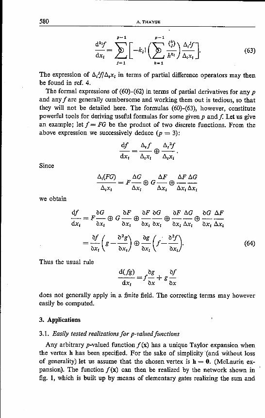
580 A.THAYSE

dk'.f = ~ [-k,! (~ (:») /),,/IJ.dx, L Lh' /)",x,

)=1 11=1

(63)

The expression of /),,/f/ /)",x, in terms of partial difference operators may thenbe found in ref. 4.The formal expressions of (60)-(62) in terms of partial derivatives for any p

and any f are generally cumbersome and working them out is tedious, so thatthey will not be detailed here. The formulas (60)-(63), however, constitutepowerful tools for deriving useful formulas for some givenp and! Let us givean example; let f = FG be the product of two discrete functions. From theabove expression we successively deduce (p = 3):

df /)"t! /)",2f-=-(B--.dx, /)",x, /)",x,

Since

/)",(FG) /)"G /)"F /)"F/)"G--=F-EElG-(B--/)",x, /)"x, Sx, Sx, /)"x,

we obtain

df 'öG 'öF 'öF 'öG 'öF /)"G 'öG!:iF-=F-EEl G-EEl--(B--(B--dx, öx, 'öx, öx, öx, öx, Sx, 'öx, /)"x,

'öf ( 'ö2g

) 'ög( . 'ö2f)=- g-- (B- f--'öx, ox, 'öx, öx,

(64)

Thus the usual ruled(fg) 'ög 'öf--=f-+g-dx, öx öx

does not generally apply in a finite field. The correcting terms may howevereasily be computed.

3. Applications

3.1. Easily tested realizationsfor p-valued functions

Any arbitrary p-valued function f(x) has a unique Taylor expansion whenthe vertex h has been specified. For the sake of simplicity '(and without lossof generality) let us assume that the chosen vertex is h = O. (McLaurin ex-pansion). The function f(x) can then be realized by the network shown infig. 1, which is built up by means of elementary gates realizing the sum and


the product modulo p respectively. Let us now define the fault model whichwill be considered further on in this section.

f(x)

Fig. 1. Network realizingf(x).

Definition 4 (generalized stuck-at-fault model)

Consider a p-valued connection which may carry the set of values

P = {O, 1, ... ,p-1}.

The faults that may occur on that connection are such that(a) only a subset Pa = (XO, (Xh ••• , (Xr-l of values of P may appear at the

output of the connection;(b) if a value (Xk E Pa is applied to the connection input, then the same value (Xk

appears at the connection output;(c) if a value {3k EP and rt Pa is applied to the connection input, then a value

(Xk E Pa appears at the connection output.Let us assume that the primary input terminals are fault-free, i.e. the input

buses are fault-free but faults can occur at the inputs of the individual gates.To detect a single faulty internal connection in a cascade of p-ary exclus-ive-OR gates, it is sufficient to apply the following set of p tests (see fig. 2):Inputs:

Xn Xo Xl Xn-l

tI = 0 0 0 0t2 = 1 0 0 0

Tl* = t3 = 2 0 0 0

tp =p-l 0 0 0

Fig. 2. Cascade of exclusive-OR gates.

oo1

oo1

582 A.THAYSE

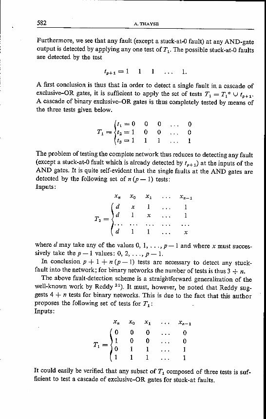
Furthermore, we see that any fault (except a stuck-at-Ofault) at any AND-gateoutput is detected by applying anyone test of Tl' The possible stuck-at-O faultsare detected by the test

1 1.

A first conclusion is thus that in order to detect a single fault in a cascade ofexclusive-OR gates, it is sufficient to apply the set of tests Tl = Tl* U tP+!'A cascade of binary exclusive-OR gates is thus completely tested by means ofthe three tests given below.

The problem of testing the complete network thus reduces to detecting any fault(except a stuck-at-O fault which is already detected by tp+ 1) at the inputs of theAND gates. It is quite self-evident that the single faults at the AND gates aredetected by the following set of n (p - 1) tests:Inputs:

Xn Xo Xl Xn-l

T, ~ )_;_

X 1 11 X 1

1 X

where d may take any of the values 0, 1, ... , p -1 and where X must succes-sively take the p - 1 values: 0, 2, ... , p - 1.In conclusion p + 1 + n (p - 1) tests are necessary to detect any stuck-

fault into the network; for binary networks the number of tests is thus 3 + n.The above fault-detection scheme is a straightforward generalization of the

well-known work by Reddy 21). It must, however, be noted that Reddy sug-gests 4 + n tests for binary networks. This is due to the fact that this authorproposes the following set of tests for Tl:Inputs:

Xn Xo Xl Xn-l

T,~)f 0 0 00 0 01 11 1 1

It could easily be verified that any subset of Tl composed of three tests is suf-ficient to test a cascade of exclusive-OR gates for stuck-at faults.

----------------------~ -- - -


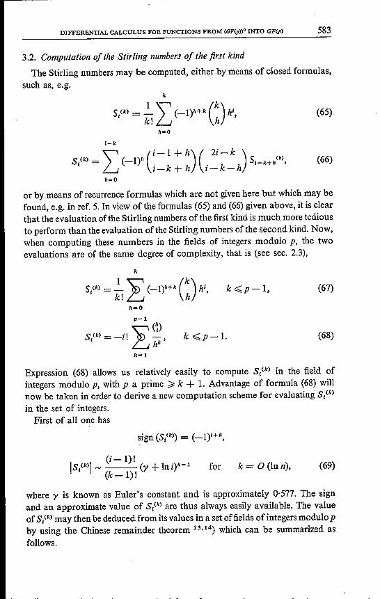
3.2. Computation of the Stirling numbers of the first kind

The Stirling numbers may be computed, either by means of closed formulas,such as, e.g.

k

SI(k) = ~!I (_I)h+k (~) hl,

h=O

(65)

I-k

SI(k) = I>-I)h C=~:~)C2i k~h) SI_k+h(h),

h=O

(66)

or by means of recurrence formulas which are not given here but which may befound, e.g. in ref. 5. In view of the formulas (65) and (66) given above, it is clearthat the evaluation of the Stirling numbers of the :first kind is much more tediousto perform than the evaluation ofthe Stirling numbers ofthe second kind. Now,when computing these numbers in the :fields of integers modulo p, the twoevaluations are of the same degree of complexity, that is (see sec. 2.3),

k

SI(k)= ~!£ (-Irk (~) hl,

h=O

p-1

(~)SI(k)=-i!~ -L...,; hk'

k~p-l, (67)

k~p-1. (68)

h=1

Expression (68) allows us relatively easily to compute SI(k) in the :field ofintegers modulo p, with p a prime ~ k + 1. Advantage of formula (68) willnow be taken in order to derive a new computation scheme for evaluating SI(k)in the set of integers.

First of all one has

(i-I)'Is (k)1'" . (r + Ini)k-1I (k-l)!

for k = 0 (Inn), (69)

where r is known as Euler's constant and is approximately 0·577. The signand an approximate value of S/k) are thus always easily available. The valueof SI(k)may then be deduced from its values in a set of:fields ofintegers modulo pby using the Chinese remainder theorem 13.14) which can be summarized asfollows.

x = bl (mod mI),x = b2 (mod m2),

(70)

584 A.THAYSE

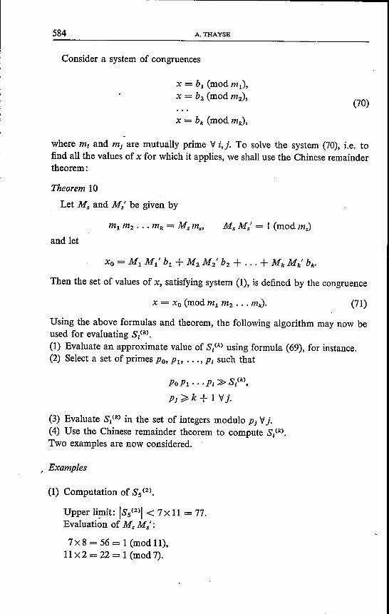
Consider a system of congruences

where mi and mi are mutually prime V i,j. To solve the system (70), i.e. tofind all the values of x for which it applies, we shall use the Chinese remaindertheorem:

Theorem 10

Let M, and Ms' be given by

and let

Then the set of values of x, satisfying system (1), is defined by the congruence

(71)

Using the above formulas and theorem, the following algorithm may now beused for evaluating S,(k).

(1) Evaluate an approximate value of S,(k) using formula (69), for instance.(2) Select a set of primes Po, Ph ... , p, such that

POP! •.. p, ~ S/k),

»,> k + 1 V j.

(3) Evaluate S/") in the set of integers modulo Pi Vj.(4) Use the Chinese remainder theorem to compute S/k).Two examples are now considered.

Examples

(1) Computation of S5(2).

Upper limit: IS5(2)1 < 7x 11 = 77.Evaluation of M; Ms' :7x8 = 56 = 1 (mod 11),11 X 2 = 22 = 1 (mod 7).


(SP» (mod 7) = -5! [(~) Ee (~)J= 6.52 62

(S (2» (mod 11)= -5! [(D Ee (~) Ee CD Et> (~) Et> (~) Ee (\O)J5 52 62 72 82 92 102

=5.x = 5x56 + 6x22 = 412.S5(2) = -(412) (mod 77)

=-50.

(2) Computation of S6(2)

Upper limit: IS6(2)1< 7 X 11X 13= 1001.Evaluation of Ms Ms':

(7X 11)X 12 = 924= 1 (mod 13),(7x 13)X 4 = 364= 1 (mod 11),(11X 13)x 5 = 715= 1 (mod 7).

(S6(2» (mod 7) = -6! [~~] = 6.

=1.

(S (2» (mod 11)= -6! [(~)Et> G) Ee (~) Et> (~) Et> cr~)J6 62 72 82 92 102

= 10.

(S6(2» (mod 13)= -6! [(~)Et> G) Ee (~) Et> (~) Et> e~)Ee el) Et> ei)J62 72 82 92 102 IF 122

=1.x = 924x 1+ 364x 10+ 715 x I= 5279.

S6(2) = (5279) (mod 1001)=274.

4. Conclusion

In this paper we have used the concepts of a partial derivative and of a totaldifferential to derive various properties of discrete functions from (GF(p»n intoGF(p). In this paper the aim has been to subsume a set of results in a singleconsistent theory very close to the classical differential calculus. However, it hasbeen pointed out that the use of appropriate computational formulas leads torather simple solutions for various kinds of problems. We have pointed out aproblem related to multivalued logic, namely the testing of p-ary Taylor ex-pansions and another problem related to numerical analysis, that is the com-

586 A.THAYSE

putation of the Stirling numbers. It seems, however, clear that the theory de-veloped in this text could be applied successfully to several other domains ofapplied mathematics such as switching theory, for instance. Further researchresults are expected in this domain.

Acknowledgement

The notion of partial derivative of a function mapping a finite field into itselfwas first introduced by my colleague Ph. Piret 22); I am much indebted to him.Thanks are also due to Dr M. Davio for constructive discussions and for sug-gesting some of the problems considered here.

MBLE Research Laboratory Brussels, October 1974

REFERENCES

1) J. P. Deschamps and A. Thayse, Philips Res. Repts 28, 397-423, 1973.2) A. Thayse and J. P. Deschamps, Philips Res. Repts 28, 424-465, 1973.3) M. Gazalé, Les structures de commutation à m valeurs et les calculatrices numériques,

Gauthier-Villars, Paris, 1959.4) A. Thayse, Philips Res. Repts, to appear.5) M. Abramowitz and I. Stegun, Handbook of mathematical functions, US National

Bureau of Standards, 1964.6) Ch. J. de la Vallée Poussin, Cours d'analyse infinitésimale, Gauthier-Villars, Paris,

1959, tome I.7) Z. Tosic, Analytical representations of m-valued logical functions over the ring of

integers modulo m, publications de la faculté d'électrotechnique de l'université à Belgrade,série: Mathématiques et Physique, no. 410-411,1972.

8) D. H. Green and I. S. T'ayl o r, Proc. lEE 121, 409-417, 1974.9) M. Davio, A. Thayse and G. Bioul, Philips Res. Repts 27,386-403,1972.

10) G. Bioul and M. Davio, Philips Res. Repts 27, 1-6, 1972.11) B. Bernstein, Modular representations offinite algebras, Proc. Intern. Math. Congress,

Toronto, University of Toronto Press, 1924, vol. 1, pp. 207-216.12) S. B. Akers, J. SIAM 7, 487-498, 1959.13) I. M. Vinogradov, An introduetion to the theory of numbers, Pergamon Press, 1961.14) L. E. Dickson, Introduetion to the theory of numbers, Dover Publication, 1957.15) A. Thayse, Philips Res. Repts 26, 229-246, 1971.16) A. T'h ays e and M. Davio, IEEE Trans. Comput. C-22, 409-420, 1973.17) M. Davio, Ring-sum expansions of Boolean functions, Symposium on Computers and

Automata at the Polytechnic institute of Brooklyn, 1971, pp. 411-418.18) D. Green and R. Kelsh, The Computer Journal16, 360-367, 1973.19) S. Lee and E. Lee, IEEE Trans. Comput. C-21, 312-319, 1972.20) D. H. Green and K. R. Dimond, Proc. lEE 117, 56-60, 1970.21) S. M. Reddy, IEEE Trans. Comput. C-21, 1183-1188, 1972.22) Ph. Piret, Derivatives of discrete functions, Private communication.

differential calculus for functions from … bound... · differential calculus for functions from...

Documents