diet quality and calories consumed: the impact of being hungrier, busier and eating out

Working Paper 04-02 The Food Industry Center

University of Minnesota Printed Copy $25.50

DIET QUALITY AND CALORIES CONSUMED: THE IMPACT OF BEING HUNGRIER,

BUSIER AND EATING OUT

Lisa Mancino and Jean Kinsey

March 2004

Lisa Mancino, Economic Research Service, USDA, 1800 M Street, Room N4083, Washington, DC 20036-5831 Jean Kinsey, Professor, Department of Applied Economics, and Co-Director, The Food Industry Center, University of Minnesota, St. Paul, MN 55108-6040, e-mail: [email protected]. The work was sponsored by The Food Industry Center, University of Minnesota, 317 Classroom Office Building, 1994 Buford Avenue, St. Paul, Minnesota 55108-6040, USA. The Food Industry Center is an Alfred P. Sloan Foundation Industry Study Center.




ABSTRACT

While Americans claim to be eating better and improving their understanding of diet and health,

they are getting heavier and increasing their risk of suffering from diet related illnesses. The

cause of this inconsistency is unclear. Using theoretical models of preference reversal and

econometric empirical analysis, this study finds that the number of calories eaten per meal

increases and the quality of the diet decreases as people wait more than six hours to eat their next

meal, work more than fifty hours a week, and consume a larger amount of food away from home.

These situational factors are important even for consumers who have considerable knowledge

about diet and health.

Regardless of one’s favored dietary prescription, this study shows how well an

individual’s intentions to eat healthfully changes with time pressures, hunger, and food source.

As people change their dietary goals based on prevailing nutritional lore, such situational factors

will continue to interfere with one’s long-term health objectives. This is especially relevant in an

era where obesity is a leading health issue for individuals and for the costs of health care. Any

advice and action that can improve diet quality and reduce caloric intake on a convenient basis is

valuable for individuals and the overall economy.

Working Paper 2004-02 The Food Industry Center University of Minnesota

DIET QUALITY AND CALORIES CONSUMED:

THE IMPACT OF BEING HUNGRIER, BUSIER AND EATING OUT


Copyright © 2004 by Lisa Mancino and Jean Kinsey. All rights reserved. Readers may make verbatim copies of this document for non-commercial purposes by any means, provided that this copyright notice appears on all such copies. The analyses and views reported in this paper are those of the authors. They are not necessarily endorsed by the Department of Applied Economics, by The Food Industry Center, or by the University of Minnesota. The University of Minnesota is committed to the policy that all persons shall have equal access to its programs, facilities, and employment without regard to race, color, creed, religion, national origin, sex, age, marital status, disability, public assistance status, veteran status, or sexual orientation. For information on other titles in this series, write The Food Industry Center, University of Minnesota, Department of Applied Economics, 1994 Buford Avenue, 317 Classroom Office Building, St. Paul, MN 55108-6040, USA; phone (612) 625-7019; or E-mail [email protected]. Also, for more information about the Center and for full text of working papers, check our World Wide Web site [http://foodindustrycenter.umn.edu].

TABLE OF CONTENTS

Introduction and Problem Statement ...........................................................................................4

Theoretical Model.......................................................................................................................7

Econometric Model...................................................................................................................17

Empirical Estimation ................................................................................................................24

Results ......................................................................................................................................25

Conclusion, Recommendations, and Future Research................................................................33

Appendix A ..............................................................................................................................36

Appendix B...............................................................................................................................37

Study Limitations and Further Research....................................................................................37

References ................................................................................................................................39

FIGURES

Figure 1: Effect of Increasing Hunger on Leisure Time........................................................ 14

Figure 2: Effect of Increasing Hunger on Food Preparation Time......................................... 15

Figure 3: Effect of Increasing Hunger on Food Consumption with mTf * =0.......................... 16

Figure 4: Interaction among Health Information, Hunger and HEI score.............................. 32

Figure 5: Interaction among Health Information, Food Source, and HEI score..................... 32

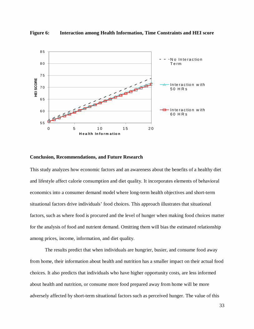
Figure 6: Interaction among Health Information, Time Constraints and HEI score............... 33

TABLES

Table 1: Variables and Definitions ..................................................................................... 20

Table. 2: Variables Used to Construct Information Index*Results ....................................... 22

Table 3: Determinants of Diet Quality (Healthy Eating Index)............................................ 26

Table 4: Determinants of Caloric Demand.......................................................................... 27

Table 5: Relative Difference of the Effect of Information on Diet Quality .......................... 31

4



Introduction and Problem Statement

Over the past twenty years, the standard public policy approach for convincing Americans’ to

adopt healthy lifestyles has centered on disseminating information about the benefits of eating

well. Numerous national campaigns have aimed at educating Americans on the importance of a

healthful diet: Consume “Five a Day” for fruits and vegetables; Follow the food guide pyramid;

Limit the percent of your daily calories from fat. The success of these campaigns has likely

contributed to the growing number of shoppers who admit their grocery purchases are affected

by health concerns and believe eating well is a better way to manage their health than medication

(FMI 2001).

Despite our increased understanding of the link between diet and health, our aggregate

diets do not seem to be leading to better health. Recently both academic journals and the popular

media have been filled with reports that describe the recent trends in obesity by using terms like

epidemic and crisis. To recap some of the key, often cited numbers as of 2003, 65 percent of all

Americans are overweight and over one-third are obese. Within the past ten years, the number of

individuals classified as obese has increased by 74 percent (CDC, 2004). 1 During this same time

span, there has been a parallel rise in the incidence of diseases highly correlated with poor

nutrition and over consumption: cancer, strokes, heart disease and diabetes. According to the

Surgeon General, obesity accounts for $117 billion a year in direct and indirect economic costs,

1 An individual is classified as obese if his or her Body Mass Index (BMI), or ratio of one’s weight in kilograms to one’s squared height in meters exceeds 30. An individual with a BMI between 25 and 30 is classified as overweight.

5

it is associated with 300,000 deaths each year, and will soon overtake tobacco as the main cause

of preventable deaths (Surgeon General, 2004).

While Americans claim to be eating better and improving their understanding of diet and

health, they are getting heavier and increasing their risk of suffering from diet related illnesses.

The cause of this inconsistency is unclear. It may be that Americans just eat too much of

everything. There may be a clear division between the people who eat poorly and the people who

eat healthfully. Alternatively, it may be that individuals try to incorporate their beliefs about

healthy eating into their food choices, but sometimes forego good intentions for more immediate

gratification because of time constraints, hunger, and a demand for convenience.

A rift between long-term objectives and short-term desires can lead to preference

reversals and time-inconsistent choices, where individuals make selections, perhaps under

pressure or in haste, which would not have been made with an objective perspective and longer

time horizon. They may drive over the speed limit when late for a meeting, drink too much wine

at a party, or opt to super-size at the drive-through window. If some food choices prove to be

time-inconsistent, then our understanding of the relationship between health knowledge and diet

quality can be improved by including factors that increase one’s demand for immediate

gratification.

Despite the mounting evidence that shorter time delays are correlated with inconsistent

choices, traditional economic studies of consumer behavior have relied primarily on prices,

income, and information to explain observed food choices. Advances in behavioral economic

theory suggest that incorporating factors, such as the delay between alternative activities and

one’s sensitivity to time-delay into consumer choice analysis will further clarify the link between

intentions and actual behavior (Hoch and Loewenstein; Frederick, Loewenstein, and

6

O’Donoghue; Loewenstein; Baumeister; Mullainathan and Thaler; Loewenstein and Elster;

Thaler). It may be that when an individual is hungry and pressed for time, one’s short-term

demand for convenience and relief from hunger may supercede long-term health objectives.

Since convenient foods are often high in calories, fat, simple carbohydrates, cholesterol, and

sodium, there is an ancillary increase in the consumption of these nutrients.

Not accounting for one’s level of hunger and demand for convenience may lead to a

misspecification of the roles of prices, income, and information on nutrient demand. In turn, this

can lead to misguided public intervention programs meant to improve nutrition, diet, and health.

A better understanding of how situational factors impact food choices will provide additional

avenues for public intervention programs aimed at improving food choices and ultimately

reducing the incidence of obesity. Knowing when individuals are apt to forego health concerns

can be used to suggest ways to avoid such situations. Alternatively, this knowledge can be used

to suggest effective commitment mechanisms that would compel individuals to make choices

that are more harmonious with their long-term health goals.

This study develops a theoretical consumer choice model that allows one’s demand for

convenience to change with time pressures and hunger. Using empirical evidence, the results

show that situational factors influence food choices and that the use of nutritional information

changes as one becomes hungrier, busier, and eats more foods away from home. The results of

this analysis can be used to inform policy recommendations on effective ways to improve diet

and nutrition.

Before proceeding, it should be noted that while many nutritionists continue to advocate a

low fat diet where the majority of calories are derived from complex carbohydrates such as

vegetables and whole grains, a high protein, higher fat diet has gained popularity as an effective

7

means for weight reduction. This debate shows that knowledge about what constitutes a healthful

diet is not static. Thus this study will utilize a flexible definition of health information to

determine how an individual’s attitudes, beliefs, perceptions, and knowledge about what

constitutes a healthful diet influence food choice. And because our impression of a healthful diet

is evolving, this study will analyze an individual’s consumption of total calories and overall diet

quality.

Finally, although the impetus for this study is to determine economic factors behind

obesity, the analysis will focus on individual food choices. The reason for this is twofold. First,

food choices play a large role in determining body weight. Second, although situational factors

are likely to affect both body weight and food choices, the effect will be more immediate on food

choices and thus, empirically more observable.

Theoretical Model

The theoretical model in this study begins with the Becker (1965) household production model,

where individuals are assumed to maximize utility, subject to their ability to produce goods and

services for personal use, their budget constraint, and the constraints on their time. To more

closely depict how individuals make their food choices, the model in this study also draws from

a growing literature on behavioral economics and allows individual’s choices to be effected by

time-delay, hunger, and other situational factors. Several behavioral-economic studies that have

incorporated sensitivity to delayed outcomes have employed a quasi-hyperbolic discount

function, similar to the one below.

(1) ∑=

+=+=T

tt

tt UUUMax

11δβ .

8

By allowing individuals to be more sensitive to time delays that occur sooner rather than later,

this relatively simple depiction captures a key feature of dynamic choice models and allows for

consumption choices to be inconsistent over time. However, as noted by Loewenstein (1996) a

limitation of this model is that hyperbolic discounters will always exhibit impulsive behavior

when time delays are short. An implication of this is that the hyperbolic model cannot account

for an individual who behaves impulsively in one situation and exercises more control in

another, even if the reward values and time delays are the same in both situations. For example, a

hyperbolic discounting model would predict that an individual would always choose the more

immediately available food alternative, regardless of his or her level of hunger. To address this

shortcoming, he advocates the inclusion of “visceral” influences, such as hunger, thirst, and pain,

into an individual’s instantaneous utility function.

The model in this study incorporates the idea of visceral influences to depict how

individuals’ food choices are affected by time delays and situational factors. Specifically, an

individual in this model makes consumption decisions on a per-meal basis (m) over some finite

planning period that ends at M. Utility is derived from food ( mF )2, a composite non-food item

(NFm), leisure time (TLm) and the individual’s perceived health status ( mH ) (Grossman). For

simplicity, the utility function is assumed to be separable in all arguments. It is assumed to be

strictly increasing and linear in health and the composite non-food item. With respect to food and

leisure consumption, the utility function is assumed to be continuous, twice continuously

differentiable, strictly increasing, strictly concave, and satisfy the Inada conditions.

2Fm is the total amount of food consumed at m, measured in grams.

9

A vector of relevant visceral factors ( mα ) experienced at the time the individual makes

his or her consumption decision influences the level of utility received. To isolate the effects of

situational factors on food consumption decisions, it is assumed that visceral factors only

influence the utility derived from food and leisure. Thus, increasing the level of hunger

experienced at time m will increase the utility garnered from food and leisure time, but will not

affect enjoyment derived from health or non-food. Individuals are assumed to be naïve and treat

these visceral factors )( mα as exogenous

(2) ( ) ( )∑=

++++++=M

mmmmmmmmmmm TLFHNFUTLFHNFUU1

);,(,,);,(,,τ

ττττττ αδα .

The utility received from health is assumed to be a strictly increasing, linear function of how

much an individual knows about health and nutrition (η ):

(3) mm H)H(U ⋅= η .

This allows people who know more about the links between diet, nutrition, and health to

perceive a greater health impact from a change in body weight than individuals who know little

about diet and health. An individual’s perceived health at time m is a function of how much that

individual weighs (wm). Weight is assumed to have a positive impact on health up to some point

W* and a negative impact thereafter. The change in weight at time m is a strictly increasing,

linear function of the difference between the number of calories (or nutrients) consumed (Km-1)

and the number of calories expended (Em-1)3. This leads to the following health production

function:

(4) )EK,w(hH 1m1m1mm −−− −= .

3 For simplicity, it is assumed that Em is exogenous. This prevents the model from allowing extreme exercising to balance caloric intake.

10

Individuals in this model transform the foods they eat, such as a hamburger and French fries, into

calories, fat and protein through a vector of coefficients ( mε ). It draws from the Lancaster (1966)

framework, where mjε can be interpreted as the amount of the jth nutrient contained in ( mF ). It

dictates an individual’s perception of how much of a specific characteristic flows from the foods

he or she consumes. Consequently, individuals in this model manage their health through the

amount of calories and nutrients that they think they have consumed, not the amount they have

truly consumed. Because individuals frequently underestimate the fat and caloric content of

foods prepared away from home (Kennedy et al), this model assumes that the accuracy of this

coefficient vector increases with the amount of time spent preparing food at home. As such, the

level of error in the vector of coefficients is assumed to be strictly decreasing and convex in the

amount of time an individual spends preparing food ( mTf ). This allows individuals to more

accurately assess the nutrient content of food they prepare than food prepared by someone else

so that the perception of calories consumed in period m are adjusted by the amount of time spent

preparing the food at time m.. In this framework then, the foods consumed are translated into

calories and nutrients in the following manner:

(5) )(ˆmmm TfFK ε⋅= .

Thus, the health production function, (4), to be rewritten as:

(4’) ( )1m1m1m1mm E)Tf(F,whH −−−− −⋅= ε ,

where health is a function of last periods body weight, perceived caloric intake and energy

expenditures.

11

Within each planning period, individuals decide how to divide their total available time4

( mTT ) between working (TYm), preparing food ( mTf ), and leisure (TLm). The amount of time

spent preparing food is assumed to increase as a function of the amount of food consumed ( )mF 5.

The per-period time constraint is:

(6) mmmmm TTTLFTfTY =+⋅+ .

Within each planning period, an individual decides whether to spend his or her income on food

or non-food. PNF is the price of non-food and PF is the price of food. With a wage rate of y,

individuals face the following per-period budget constraint:

(7) TYyFPNFP mFmNF ⋅≤+ .

Food prices typically increase with the level of pre-preparation. For example, the cost of a raw

egg is typically around $0.10, while the cost of a hard-boiled egg is around $0.75. To account for

this relationship, this model explicitly assumes that the monetary price of food decreases with the

amount of time spent in food preparation in the following way:

mFF bTfPP −= ~ .

FP~ is the monetary cost of a fully prepared, ready to eat food item. minP is the lower limit on

food prices and is the price of raw materials6. The price-savings from spending an additional unit

of time preparing food is b. Using the preceding egg example, if it took one unit of time to

prepare a hard boiled egg, then b would be equal to $0.65. Normalizing the price of non-food to

4 Total available time is the amount of time in a day, less time required for sleep. 5 For simplicity, it is assumed that food production technology exhibits constant returns to scale. 6To ensure that individuals do not sell food they produced, it is assumed that 0< mTf < ( FP~ -Pmin)/b.

12

one and making it the numeraire, the time, and budget constraint can be combined into the full-

income constraint:

(8) mmmmmmFm TLyFTfyTTyFbTfPNF ⋅−⋅⋅−⋅=⋅−+ )~( .

Rearranging (8), the composite non-food item can be expressed as a function of prices, wages,

and the amount of food consumed at time m:

(8’) mmFmmmmm FbTfPTLyFTfyTTyNF ⋅−−⋅−⋅⋅−⋅= )~( .

Substituting the health production function (4’) and the full-income constraint (8’) into (2), the

individual’s inter-temporal optimization problem becomes:

( )( )( ).),,(,)(,,(

));,(,)),)~(()9(

11111∑

=+++−+−+−+−++ −⋅+

⋅−−−⋅−=M

mmmmmmmm

mmmmmmFmmmmm

TLFETfFwhNFU

TLFHFbTfPyTLFyTfyTTUUMAX

τττττττττ

τ αεδ

α

Because the maximization problem is finite-dimensional and the constraint set is closed and

bounded, the Bolzano-Weierstrass theorem guarantees that a solution to the maximization

problem exists. Thus, the maximization problem is well defined. Furthermore, because the

constraint set is convex, the utility function is strictly concave and satisfies the Inada conditions,

the first order conditions are both necessary and sufficient to ensure that the maximization

problem yields a unique solution. Optimizing (9) with respect to the variables Fm, TLm, and mTf

13

yields the following first order conditions:

[ ]

[ ]

[ ]

.,00 (9c)

,,00);( (9b)

,,00)(

),()~( (9a)

*

1

**

*

*

1

***

MmFTf

wwh

bFFyTfU

andMmTLUyTLU

MmTfF

wwh

FUbTfPTfyFU

mm

mM

m

m

m

mmm

m

m

mmTLm

m

mm

mM

m

m

mmFmFmm

m

∈∀≤⋅∂∂

∂∂

∂∂

++⋅−=∂∂

∈∀=+−=∂∂

∈∀=⋅∂

∂∂∂

++−−⋅−=∂∂

∑

∑

=

+

+

+

+

= +

+

εε

ηδ

α

εηδ

α

τ

τ

τ

ττ

τ

τ τ

ττ

Solving for Food (Fm), Leisure Time (TLm), and Food Preparation Time ( mTf ) and substituting

the utility maximizing levels of F*m and mTf * into the (5) yields the reduced form demand

function for nutrients and/or calories:

).,,,,,,~(ˆ(10) 1−= mmmmFK

m wEybPDK ηα

Equation (10) implies that nutrient demand will be a function of prices, price savings, wages,

visceral factors (hunger), information, physical activity, and one’s body weight.

Equation (9b) shows that in equilibrium yTLU mmTL =);( * α . This implies that increasing the

level of hunger experienced at m will increase the optimal level of leisure time because

0),(2

>∂∂

∂αα

TLTLU and thus, increasing mα increases TLU . As shown in Figure 1, this suggests that

an increase in mα to mα̂ will lead to an increase in the optimal amount of mTL* to mTL ** .

14

Figure 1: Effect of Increasing Hunger on Leisure Time

Assuming 0* >mTf , equation (9c) shows that optimality implies that an individual will

equate the marginal benefits of time spent preparing food to the marginal cost. For someone

whose weight exceeds W*, (9c) can be rewritten as:

);*();( **

1mmmmTLmmTL

m

mM

m

m

m

m TfTyTTUTLUyTf

wwhb αα

εε

ηδτ

τ

τ

ττ −−===∂∂

∂∂

∂∂

+ ∑=

+

+

+ .

Thus, the marginal cost of an extra unit of food preparation time is the loss of time spent in

leisure. If hunger increases, the marginal cost of preparing food will also increase. As shown in

Figure 2, increasing hunger from mα to mα̂ will decrease the optimal amount of mTf * to mTf **

y

TLm* TLm

**

$

),( mmTL TLUMB α=

MCTL

)ˆ,( mmTL TLUMB α=

TLm

15

Figure 2: Effect of Increasing Hunger on Food Preparation Time

)ˆ,( mmTL TLUMC α=

Finally, (9a) illuminates how increasing hunger at meal m will influence overall food

consumption at that meal: In equilibrium, an individual will equate the marginal benefits of food

consumption to the marginal cost. For someone whose weight exceeds W*, (9a) can be rewritten

as:

(9a’) )()~(),( *

1

***m

m

mM

m

mmmFmmmF Tf

Fw

whbTfPyTfFU εηδα τ

τ τ

ττ ⋅∂

∂∂∂

+−+= +

= +

+∑ .

If mTf * =0, then increasing mα will lead to a higher value of ),( *mmF FU α and have no effect on

the right hand side of (9a’). Thus, to satisfy the first order conditions, an individual will increase

mF * until (9a’) holds with equality. As shown in Figure 3, increasing the level of hunger from

mα to mα̂ will increase the optimal level of food consumption from mF * to mF ** .This result is

important. If an individual decides that the optimal amount of food preparation time at meal m is

zero, then he or she will likely purchase food that is already prepared. This suggests that the

**m

Tf *m

Tf mTf

$

),( mmTL TLUMC α=

mTfmM

m

mw

mwmh

bMB∂

∂∑= ∂

+∂

+∂+∂

+=ε

τ ετ

τ

τητδ1

16

effect of hunger on the amount of food chosen will be greater for food prepared away from home

than food prepared at home.

Figure 3: Effect of Increasing Hunger on Food Consumption with mTf * =0

The effects of hunger on optimal food consumption is ambiguous when mTf * >0. From Figure 2,

increasing mα will decrease mTf * . Buying food that is more prepared may lead to a decrease in

future health and an increase in the current monetary cost. However, reducing mTf * will

decrease the marginal time cost of preparing food. As mα increases, the perceived opportunity

cost of preparing foods, ));(( *mmTL TLU α , increases as well. Thus, it is possible for the total

change in the marginal cost of increased consumption caused by an increase in mα to be

negative, zero, or positive. Nevertheless, as long as the positive change in the total marginal

benefit exceeds the total increase in marginal cost, the optimal level of food consumption will

increase with hunger. How much an individual knows about health and nutrition mη , the price

Fm* Fm

**

$

),( mmF FUMB α=

)0(1

~ ετ

τ

τ

τητδ ⋅∑= ∂

+∂

+∂+∂

+=M

mFmw

mwmh

FPMC

)ˆ,( mmF FUMB α=

Fm

17

savings from preparing one’s own food (b), and the opportunity cost of one’s time (y) all impact

the likelihood that increasing hunger mα will increase mF * . Overall, the equilibrium conditions

suggest that hunger will have a significant and positive impact on nutrient demand when:

1. An individual consumes food prepared away from home;

2. The price savings from food preparation are low;

3. The opportunity cost of time is high; and

4. An individual has less knowledge about health and nutrition.

Econometric Model

With observations on ‘i’ individuals who consumed m meals, the following functional form is

used to estimate per-meal nutrient and caloric demand:

eXK += ')12( β ,

where K is a J×1 7 vector of observations on actual per-meal nutrient consumption, β is a

n×1 vector of coefficients, X is an Jn× matrix of explanatory variables, and e is a J×1 error

vector. However, changing the unit of observation on nutrient and caloric consumption to a per-

meal basis transforms what would normally be a cross-sectional data set into a panel data set.

Using OLS to estimate nutrient demand with such data may yield inefficient parameter estimates

because individuals reporting more than two eating occasions on a single day would provide at

least two observations for estimation. Another econometric issue stems from the fact that hunger

can be influenced by the amount of food consumed at the previous eating occasion. Not

accounting for this relationship could also lead to inefficient parameter estimates because the

7 J is equal to the total number of observations, or the number of individuals, multiplied by their number of eating occasions.

18

disturbance term from the past eating occasion may be correlated with the error term from the

current eating occasion.

To circumvent these econometric issues, this study estimates the mean relationship

between the dependent and explanatory variables for a single individual. This allows (12) to be

rewritten as follows:

iii eXK += ')13( β ,

where ‘i’ denotes the individual, iK is the average per-meal level of consumption, iX is a the

per-meal average value of the n explanatory variables, and ie is the per-meal average error. With

this functional form, OLS estimation techniques should yield both consistent and efficient

estimates. Another benefit of averaging per-meal nutrient demand over the two days of intake is

that it provides a better idea of how a series of choices affects overall nutrient intake and how

people balance their caloric and nutrient consumption over an entire day. A third benefit of

averaging per-meal factors and outcomes is that it allows for the use of the Healthy Eating Index

(HEI) as a dependent variable. This index summarizes an individual’s diet quality over an entire

day. The components that comprise this index are an individual’s servings of fruits and

vegetables, carbohydrates, fat, protein, cholesterol, and overall variety in their diet (Bowman et

al).

Another econometric issue is that several of the right hand side variables, namely health

information, hunger, and food source, are arguably endogenous. As such, these variables will be

correlated with disturbances and may yield biased and inconsistent parameter estimates. The

standard econometric method of correcting for problems of measurement error and endogeneity

is to use some type of instrumental variables (IV) estimator. This requires that one find variables

that are highly correlated with the endogenous explanatory variables and not correlated with the

19

error term in the equation being estimated. However, the low correlation among variables means

that IV estimators may still be biased and inefficient (Park and Davis). For that reason, this study

employs both IV and OLS estimates. This study uses STATA 7.0 and specifies the survey’s

primary sampling unit, the level of stratification, and sampling weight to account for the data’s

complex survey design. The resulting parameter estimates will be more efficient than those that

would have resulted from simply using either OLS or IV estimators.

This study estimates the effects of information and situational factors on the demand for

overall calories and the demand for overall diet quality, measured by an individual’s HEI score.

When estimating the demand for calories, the dependent variable is the two day average of the

total calories an individual consumed at each eating occasion divided by that individual’s total

recommended daily allowance (RDA). When estimating overall diet quality, the dependent

variable is the individual’s average HEI score for the two days of intake. Summary statistics are

reported in Table 1.

The theoretical model developed in this study suggests that per-meal nutrient demand

will be a function of food prices, an individual’s wage rate, body weight, caloric expenditures,

information about health and nutrition, per-meal situational factors that affect one’s sensitivity to

time delay, and the amount of time spent preparing the meal. A limitation of this data set is a

lack of information on both food prices or food expenditures. However, when individuals’ intake

choices are made within a short time frame it is standard practice to assume that the modicum of

variation in prices across households can be captured by information on the household’s regional

location (Variyam et al, 1995, 1996). Thus, geographic location and whether or not an individual

lives in an urban, suburban, or rural area are included to represent minor fluctuations in food

20

Table 1: Variables and Definitions

Category Variable Definition Mean Std. Dev Dependent Variable

Dcals HEI

Calories at meal as a percent of RDA Individuals HEI score, 2 day intake average

0.288 62.91

0.115 11.77

Wage Rate:

Income Size School

Total household income in $1,000 Number of members in household Level of schooling: 1 if less than high school

2 if high school or GED 3 if some college

4 if at least four years of college

34.88 2.586 0.170 0.339 0.169 0.229

26.37 1.464 0.375 0.473 0.374 0.420

Food Prices and Expenditures

Midwest South West Northeast Urban Suburban Rural

1 if Midwest 1 if South 1 if West 1 if Northeast 1 if central city 1 if suburb 1 if rural

0.252 0.355 0.203 0.191 0.296 0.437 0.267

0.434 0.479 0.402 0.392 0.457 0.496 0.442

Body Weight and Caloric Expenditures

BMI Female Activity Active job BFPL TV Age

Body weight (kgs)/ height2 (meters 1 if individual is female; 0 otherwise Stated activity level:

1 if less than 3 times pre month 2 if 1-4 times per week 3 if at least 5 times per week

1 if individual has a job that is physically demanding; 0 otherwise 1 if pregnant, breast feeding or lactating Average hour of t.v. watching per day Age of meal-planner in years

28.09 0.496 0.442 0.290 0.265 0.224 0.009 2.667 50.88

11.82 0.500 0.497 0.451 0.441 0.417 0.095 2.176 17.19

Demand Shifters

Vegetarian Smoker White Black Hispanic

1 if vegetarian 1 if smoker 1 if White 1 if Black 1 if Hispanic

0.030 0.257 0.776 0.115 0.081

0.171 0.437 0.416 0.318 0.272

Situational Factors and Sensitivity to time delay

Interval Breakfatst0 Brekfast1 Breakfast2 Snack Meal

Time elapsed between meals 1 if no breakfast on day 1 or day 2 1 if only one day with breakfast 1 if breakfast on both day1 and day2 1 if previous eating occasion was a snack 1 if previous eating occasion was a meal.

4.104 0.058 0.156 0.786 0.336 0.677

1.422 0.234 0.363 0.410 0.179 0.182

Food Source: Free Captive Cheap Social Planned

1 if meal came from someone else 1 if meal came from cafeteria, dining center 1 if food came from fast food restaurant, pizza place, vending machine 1 if meal came from a sit down restaurant or bar 1 if meal came from a grocery store

0.076 0.022 0.083 0.064 0.713

0.137 0.079 0.133 0.120 0.098

Information Information Beliefs Perceptions Awareness

See Table 5.2 5.993 4.619 7.022 7.605

1.668 1.378 1.296 1.390

21

prices and expenditures. The household income for a given individual, the size of that household,

and an individual’s level of education are included to provide data on an individual’s wage rate.

An individual’s BMI and gender are included to provide information about an

individual’s body weight and caloric expenditures. The rationale for including these variables is

that BMI should be highly correlated with weight, and all else equal, women tend to weigh less

than men. An individual’s reported level of physical activity, whether or not the individual has a

physically demanding job (Kuchler and Lin), and whether or not an individual is pregnant,

lactating or breastfeeding are all factors that will increase ones caloric expenditures. Conversely,

the number of hours of TV watched per day and an individual’s age should be negatively related

to one’s caloric expenditures.

An individual’s ethnicity, whether or not an individual is a vegetarian, and whether or not

the individual currently smokes cigarettes are included as additional explanatory variables in the

per-meal nutrient and caloric demand functions. It is hypothesized that these variables may act as

demand shifters. Nicotine is reported to be an appetite suppressant, thus smokers will likely eat

less at each meal. Due to the nature of their diets, vegetarians are likely to consume less fat and

protein at each meal. Because individuals from different ethnic backgrounds may have very

diverse dietary habits, ethnic differences may also cause significant variation in per-meal caloric

and nutrient consumption.

Responses from the Diet Health Knowledge Survey (DHKS) (Appendix A) are used to

create an index to measure knowledge about health and nutrition for each individual. Typically,

such an index is constructed by summing the number of questions an individual answers

correctly about the links between diet and health. However, as the marketing axiom suggests,

perception is reality; what someone perceives to be true is likely to be a better predictor of

22

behavior than simply whether or not someone believes what experts maintain as true. Because of

this, health information is grouped into four general categories: information, beliefs, perceptions,

and importance (Table 2). Justification for this is based on a theory of human behavior developed

for marketing that links beliefs and attitudes to observed behavior (Fishbein and Manfredo).

Using this framework illuminates how different aspects of information are used when making

food choices. For example, although a consumer may be fully aware of the links between being

overweight and health problems, if she does not think it is important, she will be less likely to act

on this information.

Table. 2: Variables Used to Construct Information Index*

Objective Information Subjective InformationKnowledge Beliefs Perceptions Importance

5.993 4.622 7.022 7.6031.668 1.378 1.296 1.390

Number of correct answers on health questions

Agreement with 'some people are born to be fat..not much you can do..'

Perception of caloric intake Whether or not an individual is on any low calorie, low fat, low sodium, high fiber or diabetic diet.

Number of correct servings of grains, fruits, vegetables, etc. the individual is able to identify

Number of diseases associated with being overweight, eating excessive amounts of calories, fat, sodium and cholesterol.

Whether or not respondent is involved with some aspect of meal planning

Importance of maintaining a healthy weight, eating lots of fiber, eating lots of fruit and vegetables, and limiting intake of fat, sodium, and cholesterol.

Agreement with 'What you eat can make a difference in chance of getting a disease'

Perception of own body weight, health, diet quality and nutrient intake

Agreement with '.. so many recommendations.. it's hard to know what to believe'

Use of nutrition labels

*The variable's mean and standard deviation are reported below each variable's name.

23

Answers to questions that form the information index have definitive right and wrong

answers, whereas answers to belief questions are more subjective8. An example of a question

used to form the information index is whether an individual was able to identify the

recommended daily servings of vegetables. The total number of diseases a respondent attributed

to over consumption of fat, sodium, cholesterol, excessive calories, and obesity is used to

construct the beliefs index. The perceptions index is constructed by comparing how respondents

ranked their own diet quality to how their actual diet was ranked using the USDA’s Healthy

Eating Index (Bowman et al; Variyam et al, 2001, Mancino and Kinsey). Questions that asked

respondents to rank the importance they placed on maintaining a healthy weight, limiting

saturated fat, eating fiber, and limiting cholesterol are used to construct the importance index.

In order to isolate the effects of situational factors such as hunger and sensitivity to time

delay, this study analyzes nutrient intake at each eating occasion. Although the CSFII does not

explicitly ask individuals how hungry they were at each eating occasion, it does provide

information on the time elapsed between eating occasions, the individual’s classification of each

eating occasion as either a snack or a meal, and whether the individual reported eating breakfast

on either or both days of the recall. These variables are used to proxy an individual’s average

level of hunger at each meal.

Finally, the CSFII does not collect information on the amount of time an individual

spends preparing meals. Therefore, where the individual purchased or received the meal is used

to proxy the amount of time he or she spent preparing that meal. When an individual reported

more than one food source for a single meal, the food source that provided the most calories was

considered the source for that meal. There are five types of places the individual could have

8 A detailed description of the questions used to construct each component of the information index can be obtained

24

procured his or her meal, from someone else; a cafeteria, or day care center; a fast food

restaurant, pizza place or vending machine; a sit-down restaurant; or a food store, such a grocery

store, convenience store or supermarket.

Empirical Estimation

This study uses three different econometric models to estimate per meal caloric and nutrient

demand. The first model uses OLS to estimate the following average per-meal demand functions:

Model 1: OLS iiiiiiiioi

D eSFwpyK ++++++++= 7654321 ''' βαβηβεβββββ ,

where iDK is the average per-meal demand for calories, and overall diet quality (HEI)9. These

dependent variables are assumed to be linear functions of an individual’s income variables (yi),

variables that affect food prices and expenditures (pi), factors that affect an individual’s weight

and caloric expenditures (wi), other demographic characteristics (εi), an individual’s knowledge,

beliefs, perceptions, and attitudes about diet and health (η i), the average per-meal visceral

factors ( iα ), and the proportion of meals that came from a fast-food restaurant, a full-service

restaurant, a grocery store, a cafeteria, or someone else ( iFS ).

The theoretical model developed in this study suggests that the variable ‘Food Source’

should be considered endogenous. Thus, the second model in this study uses whether or not an

individual received food stamps or participated in the WIC program to instrument the portion of

food prepared at home. The rationale behind this is that these programs limit the amount of

money spent on foods prepared away from home. For example, food stamps can be used to buy

from the authors. 9 Observations are averaged over both days of intake.

25

ground-beef and hamburger buns, but they cannot be used to buy a hamburger at a restaurant,

deli, or fast-food place. Using these two variables as instruments requires a change in the

empirical model employed in Model 1 because there are insufficient instruments to partition food

sources beyond food at home and food away from home. For this reason, Model 2 has only one

variable for (FS*i). This variable measures the share of eating occasions that consisted of foods

prepared at home. This study uses two-staged least squares for the IV estimation. In the first

stage, the variable home is regressed on the instrumental variables plus all other exogenous

variables included in Model 1. Within Model 2, the demand functions are estimated twice, once

using an IV estimator and once using an OLS estimator. This is done to provide more

consistency between the models with and without instruments. Statistical tests suggest that there

is no systematic difference between the two estimators, and thus OLS estimates will be both

consistent and efficient. Subsequent description of the overall estimation results will focus on the

finding from the OLS regressions.

Results

Results from the OLS regressions are summarized in Tables 3 and 4.10 When interpreting the

results, it is helpful to know that the intercept term represents a white male who went to college,

lives in an urban area in the Northeastern United States, has a sedentary job, exercises

moderately (was not pregnant, breastfeeding or lactating) and ate breakfast on both days of the

dietary recall. The estimated OLS models explained about 30 percent of the total variation in an

individual’s two-day average HEI score (Table 3) and nearly 20 percent of the variation in the

average per-meal energy (Table 4).

10 Detailed results of the IV estimates can be found in Mancino, Lisa “Dissertation” or on request from the authors.

26

Table 3: Determinants of Diet Quality (Healthy Eating Index)

*Significant at the 5% level **Significant at the 10% level

Dependent Variable: HEIEstimated

BetaStandard

ErrorIntercept 58.193 1.978 **Income 0.0180 0.0070 **Hhsize -0.4569 0.1287 **Some High School -1.3869 0.8465High School -0.9632 0.5080 *4+ years of College 1.3097 0.5762 **Midwest 0.2540 0.5971South -1.1048 0.8266West 0.2178 0.6978Suburb -0.3501 0.4964Rural -2.3626 0.7329 **BMI -0.0377 0.0142 **Female 0.1549 0.3207Very Little Exercise -0.9276 0.4983 *Very Active -0.3094 0.3918Active Job -0.3841 0.4577BFPL 6.7365 2.1054 **TV -0.2095 0.0965 **Age 0.0738 0.0112 **Vegetarian 0.6716 1.4553Smoker -3.8763 0.4757 **Black -2.2166 0.8043 **Hispanic 2.1192 0.6910 **Information 0.4290 0.1281 **Beliefs 0.6075 0.1755 **Perceptions 0.7707 0.1800 **Importance 0.3878 0.1415 **Interval -1.7540 0.6236 **Interval2 0.0526 0.0538No Breakfast -4.7971 0.9757 **Breakfast on One Day -3.2197 0.4686 **Meal 1.0760 1.3825Other eo -1.2529 2.8519Home NA NAFree -2.2210 1.5190Captive -0.5162 2.7958Social -7.2076 1.1865 **Cheap -7.9262 1.4478 **Other -3.8103 1.8320 **

R-Squared 0.286F(37,7) 32.420

27

Table 4: Determinants of Caloric Demand

*Significant at the 5% level **Significant at the 10% level

Dependent Variable: Calories

Estim ated Beta

Standard Error

Intercept 0.2423 0.0233 **Incom e 0.0000 0.0001Hhsize -0.0031 0.0016 **Som e High School -0.0106 0.0080High School -0.0045 0.00704+ years of College -0.0134 0.0058 **Midwest 0.0103 0.0093South -0.0089 0.0094W est 0.0031 0.0068Suburb -0.0046 0.0057Rural 0.0005 0.0058BMI 0.0000 0.0002Fem ale -0.0270 0.0040 **Very Little Exercise 0.0018 0.0054Very Active 0.0117 0.0074Active Job 0.0022 0.0068BFPL -0.0066 0.0113TV 0.0053 0.0022 **Age -0.0006 0.0002 **Vegetarian -0.0107 0.0122Sm oker 0.0021 0.0065Black 0.0303 0.0138 **Hispanic 0.0019 0.0075Inform ation 0.0019 0.0014Beliefs -0.0006 0.0015Perceptions -0.0082 0.0023 **Im portance -0.0044 0.0017 **Interval 0.0254 0.0069 **Interval2 -0.0011 0.0006 **No Breakfast 0.0025 0.0113

Breakfast on One Day 0.0072 0.0079Meal 0.0929 0.0164 **Other eo 0.0239 0.0318Hom e NA NAFree 0.0805 0.0233 **Captive 0.0391 0.0248Social 0.0998 0.0172 **Cheap 0.0806 0.0378 **Other 0.0173 0.0184

R-Squared 0.207F( 37, 7) 11.860

28

Situational Factors: Analysis on variables that gauge an individuals’ level of hunger at each

eating occasion supports the hypothesis that such situational factors do have a significant impact

on actual food choices and diet quality. In all OLS estimates, increasing the interval between

eating occasions is associated with a significant decrease in HEI scores and caloric consumption.

The effect of hunger on food choices is estimated to increase caloric consumption up to some

point then significantly taper off. Evaluated at the sample means, a ten percent decrease in the

interval between meals is estimated to increase one’s HEI score by .94% and reduce per-meal

energy over 2.5%. Stated another way, decreasing the length of time between meals by 24

minutes is correlated with a 0.6 point increase in the HEI score and 15 point reduction in calories

consumed at each meal. Although this seems rather small, it should be noted that, for an

individual who consumes 3 meals a day, decreasing the interval between meals would reduce

caloric intake by 45 calories a day. Over a year, this would result in a about a five pound

reduction in total body weight, all else being equal.

Individuals who reported eating breakfast on both days of intake score significantly

higher on the HEI than individuals who skipped breakfast on at least one day of the recall. Eating

breakfast on both days is also estimated to significantly decrease the total number of calories

consumed at each eating occasion.

Health and Diet Information: Increasing the accuracy of an individual’s perceptions about

weight and diet quality significantly increases one’s HEI score and significantly decreases per-

meal caloric intake. The level of importance placed on maintaining a healthy diet also

significantly influences overall diet quality. Individuals who report placing more importance on

diet and health are estimated to have a significantly higher quality diet and consume significantly

fewer calories at each meal. Increasing the number of diseases an individual associates with

29

consuming nutrients like fat and cholesterol is estimated to significantly increase an individual’s

per HEI score. Increasing health information, measured as objective knowledge about health and

nutrition, significantly increases an individual’s HEI score.

Evaluated at the sample means, a ten percent increase in the accuracy of one’s perception

about diet quality increases the HEI score over 0.80% and decreases his average per-meal caloric

intake by over 1.8%. This translates to a little over a half point increase in his HEI score and

reduces the calories consumed at each meal by ten calories. Increasing overall health knowledge

by ten percent increases the HEI score by 1.62%, about one point, and decreases average per-

meal energy intake by 1.17%, roughly seven calories.

Food Source: Analysis on where an individual procured food for a specific eating

occasion supports the hypothesis that the source of food impacts one’s food choices and diet

quality. Increasing the share of meals obtained from fast food (cheap) or full service restaurants

(social) significantly decreases an individual’s HEI scores and significantly increases per-meal

consumption of calories compared to eating at home. Increasing the share of eating occasions

prepared by someone outside the home, such as a snack tray or a meal prepared by someone else

(free), is estimated to significantly increase per meal caloric intake.

Household Income and Household Size: There is a positive relationship between income

and diet quality. This is congruous with the theoretical assumption that diet quality is a normal

good. Individuals from larger households are significantly more likely to consume fewer calories

per meal and have a lower HEI score. Because income is often correlated with education, it is not

surprising that effect of schooling was estimated to be similar to the effect of income. Compared

to an individual who had some college, individuals with four or more years of college are

significantly more likely to have higher HEI scores and consume fewer calories at each meal.

30

Price/Geographic Location: Individuals who live in rural areas score significantly lower

on the HEI than individuals who lived in urban areas. There is no significant difference in

calories and HEI by region of the country.

Weight and Physical Activity: An individual’s reported BMI was estimated to be

negatively correlated with his or her HEI score. Females consume significantly fewer calories at

each meal. Individuals who reported very little physical activity have significantly lower HEI

scores than individuals who exercise more regularly. Women who were breastfeeding, lactating,

or pregnant (BFPL) score higher on the HEI. Increasing the amount of television watched per

day is found to have a significantly positive effect on per-meal calorie consumption and a

significantly negative effect on an individual’s dietary quality.

Additional Demand Shifters: Older individuals consume significantly fewer calories and

have a significantly higher quality diet. Smokers have lower HEI scores. Black individuals have

significantly lower HEI scores than whites, while Hispanic respondents are estimated to score

significantly higher than whites. Blacks also consume significantly more calories at each meal

than white respondents.

Interaction of Information and Situational Factors: Finally, this study tests the hypothesis

that the role of information on food choice changes as one becomes hungrier, busier, and

consumes more foods away from home. For simplicity, the four health knowledge variables are

aggregated into a single information index. From this, OLS estimates are used to gauge the joint

effect of the interval between meals and information, the portion of food consumed away from

home and information, and the number of hours worked in a week and information. Table 5

summarizes the results of this analysis by reporting each interaction term’s relative magnitude,

its estimated coefficient, and its estimated p-value in parentheses. The first row of the second

31

column of Table 5 should be interpreted to mean that the effect of information on overall diet

quality significantly decreases as an individual goes longer between meals. Overall, the results of

this analysis on the interaction term suggests that the strength of the relationship between health

information and overall diet quality wanes as an individual consumes more meals away from

home, goes longer between meals, and works more hours in a given week.

Table 5: Relative Difference of the Effect of Information on Diet Quality Relative Effect of Information on Overall

Diet Quality (HEI) when an individual

Goes Longer Between Meals Smaller** -.1468

(.006) Eats More Meals At Home Larger** .9005

(.005) Works More Hours in a Week Smaller** -.0030

(.000) **Estimated to be significant at a .05% level of significance

Figures 4 through 6 show these relationships graphically. The dashed line in Figure 4

represents how an individual’s HEI score will change with increasing levels of health

information with no interaction term. The other four lines represent how an HEI score will

respond to increasing levels of information when an individual goes two, four, six or eight hours

between meals, using the sample means in conjunction with the estimated coefficients from a

regression that includes an interaction term between health information and the interval between

meals. It shows that the HEI score rises with health information, but when the interval is six

hours or more, the HEI falls below the mean effect (dashed line). As people get hungrier, less

attention is given to healthy diets even at high levels of diet and health information. Similarly,

Figure 5 shows that an individual’s HEI score is lower when eating more meals away from

home. Working 50 and 60 hours in a given week also pushes the HEI below the mean (Figure 6).

32

Figure 4: Interaction among Health Information, Hunger and HEI score

55

60

65

70

75

80

85

0 5 10 15 20H ea lth In fo rm atio n

HEI S

core

N o In te rac tionT e rm

In te rac tion w /2 ho u rs b /wm ea lsIn te rac tion w /4 ho u rs b /wm ea lsIn te rac tion w /6 ho u rs b /wm ea lsIn te rac tion w /8 ho u rs b /wm ea ls

Figure 5: Interaction among Health Information, Food Source, and HEI score

5 0

5 5

6 0

6 5

7 0

7 5

8 0

8 5

0 5 1 0 1 5 2 0H e a lth In fo rm a tio n

HEI

Sco

re

N o In te ra c tio nT e rm

In te ra c tio n w /1 0 0 % o f F o o d A tH o m e

In te ra c tio n w / 5 0 %o f F o o d A t H o m e

In te ra c tio n w / 2 5 %o f F o o d A t H o m e

33

Figure 6: Interaction among Health Information, Time Constraints and HEI score

Conclusion, Recommendations, and Future Research

This study analyzes how economic factors and an awareness about the benefits of a healthy diet

and lifestyle affect calorie consumption and diet quality. It incorporates elements of behavioral

economics into a consumer demand model where long-term health objectives and short-term

situational factors drive individuals’ food choices. This approach illustrates that situational

factors, such as where food is procured and the level of hunger when making food choices matter

for the analysis of food and nutrient demand. Omitting them will bias the estimated relationship

among prices, income, information, and diet quality.

The results predict that when individuals are hungrier, busier, and consume food away

from home, their information about health and nutrition has a smaller impact on their actual food

choices. It also predicts that individuals who have higher opportunity costs, are less informed

about health and nutrition, or consume more food prepared away from home will be more

adversely affected by short-term situational factors such as perceived hunger. The value of this

5 5

6 0

6 5

7 0

7 5

8 0

8 5

0 5 1 0 1 5 2 0H e a lth In fo r m a t io n

HEI

SC

OR

E

N o In te ra c tio nT e rm

In te ra c tio n w ith5 0 H R s

In te ra c tio n w ith6 0 H R s

34

model is that it explicitly identifies elements that increase demand for immediate gratification

and induce behaviors contrary to one’s long run health objectives.

This research shows that although our knowledge about the importance of eating well

should increase our intentions to follow a healthy diet, our intentions can be thwarted by hunger,

a hectic schedule, and where we choose to obtain our food. Making specific reference to such

situations and suggesting ways to mitigate their effects should enhance the usefulness of

educational campaigns designed to improve diet quality. For example, disparities between one’s

intentions to eat well and his or her actual diet quality could be reduced by increasing the

convenience of foods with higher nutritional value, or by improving the nutrient content of foods

that are relatively more convenient. Another way to decrease this disparity would be to

encourage consumers to take control of the interval between meals. In turn, this will strengthen

the link between good intentions and observed behavior, while ultimately reducing the frequency

of time-inconsistent food choices.

Alternatively, planning ahead and increasing the portion of meals that are prepared with

foods from a grocery store or supermarket are also estimated to significantly decrease caloric

consumption, and improve overall diet quality. Thus, another recommendation to improve

overall diet quality would be to encourage individuals to plan ahead and make their food choices

before increasing their vulnerability to situational factors such as hunger and having the option to

super-size.

Another result of this study suggests that future nutrition campaigns should focus on

those aspects of information that have the most influence over observed behavior: importance

and perception. A more efficient way to induce change would be to help individuals become

better aware of their actual diet quality and convince them of its importance for healthy living.

35

Also, it would be beneficial to provide nutritional information on foods prepared away from

home. Although labeling laws have improved our understanding of the nutrient content of food

purchased at a grocery store, there is room to improve our understanding of foods prepared away

from home. The results of this study suggest that reducing the discrepancy between perceived

and actual diet quality would have the largest impact on improving diet quality.

Regardless of one’s favored dietary prescription, this study shows how well an individual

is able to match intentions to actually eating healthfully changes with time pressures, hunger, and

food source. As people change their dietary goals based on prevailing nutritional lore, such

situational factors will continue to interfere with one’s long-term health objectives. This is

especially relevant in an era where obesity is a leading health issue for individuals and for the

costs of health care. Any advice and action that can improve diet quality and reduce caloric

intake on a convenient basis is valuable for individuals and the overall economy.

36

Appendix A

The Data

The data used in this study comes from the United States Department of Agriculture’s (USDA) 1994-1996 Continuing Survey of Food Intake by Individuals (CSFII) 1994-1996 and the companion Diet and Health Knowledge Survey (DHKS). The purpose of the CSFII is to monitor food use and consumption patterns in the U.S. The DHKS provides information on peoples’ attitudes and knowledge about dietary guidelines and their actual ability to practice this knowledge. In each CSFII household, the DHKS was administered to one adult over 20 years old who reported at least one day of food intake. For the purposes of this study, only individuals who also answered the DHKS were included in the econometric analysis to maintain a clear link between one’s diet awareness and her nutrient intake.

37

Appendix B

Study Limitations and Further Research

There are some noteworthy limitations to this study, both in the theoretical models and the empirical application, that suggest productive avenues for future research. For one, relaxing some of the simplifying assumptions made about the theoretical model could lead to different predictions about the effects of situational factors on food choice and the use of information. For example, an individual in this model is assumed to get utility from leisure time and disutility from time spent in food preparation. However, there are certainly people who do enjoy cooking and view it as another form of leisure activity. Thus, the model could be extended to accommodate different views towards cooking. This extension could be used to predict how an individual’s views on cooking are correlated with his or her response to various situational factors, food choices, and use of health information.

Two other simplifying assumptions made in the theoretical model are that the food production technology exhibits constant returns to scale and food prepared in one period must be consumed within that period. Again, these are fairly unrealistic assumptions. Relaxing the first assumptions could provide insight into how culinary skills and household size impact an individual’s reaction to situational factors. Relaxing the assumption about food storability could be used to obtain both a theoretical and empirical measure of the value of producing more healthful meals at home, and utilizing these leftovers for future consumption.

Empirically, the most glaring limitation and promising area for future research would be to discover stronger instruments for the endogenous variables. This in turn requires more detailed data. For example, more precise information about an individual’s location could be used to get an indication of the number of fast-food restaurants, full-service restaurants, and grocery stores in the individual’s neighborhood. This would provide a better gauge of the full cost of each food alternative and relative convenience of each food source.

Also, it would be desirable to have variables that could be used to instruments for an individual’s health information. Admittedly, health information is also an endogenous variable. However, the data set lacks variables that are both highly correlated with information and theoretically exogenous. Thus, to improve future research in this area, it would be beneficial for surveys to provide additional information that could be used for instruments on health information. For example, providing more detailed information about an individual’s occupation could be used to partition individuals who worked in health care, nutrition, or medicine and those who did not. Presumably individuals who work in these areas would possess higher health knowledge. More detailed on the type of diabetes an individual had could also be used for better information instruments. Unlike Type II diabetes, Type I is genetic and not associated with bodyweight. Thus, it is theoretically exogenous. However, it still requires more detailed monitoring of diet and nutrition and should therefore be highly correlated with health information.

A third limitation of the data is that the accuracy of the food consumption information is completely dependent on the individual respondents. There are a few findings in this study that suggest there may be some shortcomings in this information. The first is that individuals who are classified as obese report consuming significantly fewer calories than individuals who are

38

considered to be overweight. This seems unlikely and suggests that respondents who were very overweight understated their true consumption.

Another anomalous finding is that Hispanic respondent’s were estimated to have significantly higher quality diets. However, in the overall population, Hispanic individuals are more likely to be overweight or obese than non-Hispanic white individuals. A plausible explanation for this incongruity is that the food tables used by nutritionists to translate foods consumed into nutrients may not accurately account for the fact that Hispanic foods tend to use more fat and lard than non-Hispanic renditions of the same food.

39

References

Baumeister, R.F., (2002) “Yielding to Tempatation: Self-Control Failure, Impulsive Purchasing, and Consumer Behavior.” Journal of Consumer Research (28) March: 670-676. Becker, G., (1965) “A Theory of the Allocation of Time,” The Economics Journal (75), September: 493-517. Bowman, S.A., M. Lino, S.A. Gerrior, and P. Bastiosis. (2002) The Healthy Eating Index:1999-2000. U.S. Department of Agriculture, Center for Nutrition Policy and Promotion. CNPP-12 http://www.usda.gov/cnpp/Pubs/HEI/HEI99-00report.pdf.

Centers for Disease Control (2003.) “1991–2001 Prevalence of Obesity Among U.S. Adults, by Characteristics.” http://www.cdc.gov/nccdphp/dnpa/obesity/trend/prev_char.htm Fishbein, M. and M.J. Manfredo (1992) “A Theory of Behavior Change.” In Influencing Human Behavior: Theory and Applications in Recreation, Tourism and Natural Resources Management. ed M.J. Manfredo. Sagamore, Champaign, IL. Food Marketing Institute, (2001a) “Reaching Out to the Whole Health Consumer.” in Prevention Magazine. Rodale Incorporated. Frederick, S., G. Loewenstein, and T. O’Donoghue, (2002) “Time Discounting and Time Preference: A Critical Review.” Journal of Economic Literature. June: 351-401. Grossman, Michael, (1972) “On the Concept of Health Capital and the Demand for Health.” The Journal of Political Economy (80), Mar-April: 223-225. Hoch, S.J and G.F. Loewestein, (1991) “Time-Inconsistent Preferences and Consumer Self Control.” The Journal of Consumer Research. (17:4) March: 492-507. Kennedy, E., S.A. Boman, M. Lino, S.A. Gerrior and P. Basiotis, (1999). “On the Road to Better Nutrition.”, in Americas Eating Habits Changes and Consequences, ed E. Frazao. Agriculture Information Bulletin Number 750, Economic Research Service, United States Department of Agriculture. Kuchler, F. and B-H Lin (2002) “The Influence of Individual Choices and Attitudes on Adiposity.” International Journal of Obesity. (26) 1017-1022. Loewenstein, G., (1996) “Out of Control: Visceral Influences on Behavior,” Organizational Behavior and Human Decision Processes. (65:3) March: 272-292. Loewenstein, G., and J. Elster Ed., (1992) Choice Over Time. New York: Russell Sage Foundation.

40

Mancino, Lisa (2003) “Americans’ Food Choices: The Interaction of Intentions, Impulses, and Convenience” Ph.D. Thesis, University of Minnesota Mancino, Lisa and Jean Kinsey (2002) “The Road to Not-So-Wellville: Paved with Good Intentions, Misperceptions, and Time Constraints.” Choices, Fall. Mullainathan, S. and R. Thaler (2000) “Behavioral Economics.” NBER Working Paper #7984. Park, J and G.C. Davis, (2001a) “The Theory and Econometrics of Health Information in Cross-Sectional Nutrient Demand Analysis.” American Journal of Agricultural Economics. (83:4) November: 840-851. Park, J and G.C. Davis, (2001b) “The Theory and Econometrics of Health Information in Cross-Sectional Nutrient Demand Analysis.” Faculty Paper Series FP 01-02, Department of Agricultural Economics, Texas A&M University, January. http://agecon.tamu.edu/publications/fp01-02.pdf The Surgeon General's Call To Action To Prevent and Decrease Overweight and Obesity http://www.surgeongeneral.gov/news/pressreleases/pr_obesity.PDF) Thaler, R.H., (1981) “Some Empirical Evidence on Dynamic Inconsistency.” Economic Letters (8):201-207. Variyam, J.N., Y. Shim, and J. Blaylock (2001). “Consumer Misperceptions of Diet Quality.” Journal of Nutrition Education. (33:6) November/December: 314-321. Variyam, J.N., J. Blaylock, and D. Smallwood (1995) “Modeling Nutrient Intake: The Role of Dietary Information.” Food and Consumer Economics Division, Economic Research Service, U.S. Department of Agriculture. Technical Bulletin No. 1842. Variyam, J.N., J. Blaylock, and D. Smallwood (1996) “A Probit Latent Variable Model of Nutrition Information and Dietary Fiber Intake. American Journal of Agricultural Economics. (78) August: 628-639.

diet quality and calories consumed: the impact of being hungrier, busier and eating out

Documents