“DIELECTRIC SPECTROSCOPY

&

Comparison With Other Techniques”

DIELECTRIC SPECTROSCOPY

• measures the dielectric and electric properties of a medium as a function of frequency (time)

• is based on the interaction of an external electric field with the electric dipole moment and charges of the medium

Dielectric properties

Complex dielectric permittivity relative to vacuum

ε*(ω)=ε’(ω)-iε’’(ω)

Complex conductivity

σ*(ω)=σ’(ω)+iσ’’(ω)

Complex electric modulus

Μ*(ω)=Μ’(ω)+iΜ’’(ω)

as a function of temperature

Medium in an external electric field

� � � �� � � � �

� � � � �Electric

Field

D=ε0εsE

•D=ε0E+P•P=ε0χsE•εs= χs+1

Medium in an external electric field

Relation between macroscopic and microscopic quantities

∑=i

ipV

P1

Dipole moments can have an induced or a permanent character

Permanent dipole moments, µInduced polarization, P

∞

∞∞ +=+= ∑ PV

NP

VP

i

i µµ1

µ Is determined by:•The interaction between the dipoles•The local electric field at the location of the dipole

Medium in an external electric field

EkT3

2µµ =

•No interaction between dipoles and local electric field equal to the outer applied fieldthermal energy �� interaction energy between the dipole and the electric field

V

N

kTs

2

03

1 µε

εε =− ∞

•Interactions between molecules, effect of polarization of environment

V

N

kTFgs

2

03

1 µε

εε =− ∞

( )( )∞

∞

++

=εε

εε

s

sF23

22

“Internal field” Onsager factor

ψµµ

cos12

2

int zg +== “Dipole interactions” Kirkwood-Froehlich factor

Onsager-Kirkwood-Froehlich equation

Langevin equation

Relation between macroscopic and microscopic quantities

Dielectric dispersion in time domain

Perturbation

Electric Field

E(t)

ε(t)

Response

Electric Displacement

D(t)

E0

0

E(t)

t

εεεεoo

εεεε0E0

0

D(t)

t

εεεε0εεεεsE0( ) ( ) 00 EttD εε=

( ) ( ) ( )tt s ϕεεεε ∞∞ −+=

( ) 00 =ϕ ( ) 1=∞ϕ

( ) ( )tt ϕ−=Φ 1

Dielectric dispersion in frequency domain

Perturbation

Electric Field

E(ω)

ε*(ω)

Response

Electric Displacement

D*(ω)

D(t)=D0sin(ϖϖϖϖt-δδδδ)

ϖϖϖϖt

E(t)=E0sin(ϖϖϖϖt)

δδδδ

( ) ( ) ( )ωωω DiDD ′′+′=*

( ) ( )ωδω cos0DD =′

( ) ( )ωδω sin0DD =′′

( ) ( )ωδε

ωε cos00

0

E

D=′

( ) ( )ωδε

ωε sin00

0

E

D=′′

Time-frequency domain

( ) [ ]dttidt

tdω

εεωε −−= ∫

∞

∞ exp)(0

*( )( ) [ ] ωωεωεπ

εdti

dt

tdexp

2

1)(

0

*∫∞

∞−=

( ) ( )[ ]tt s Φ−−=− ∞∞ 1)( εεεε

( ) ( ) [ ]dttidt

tds ωεεεωε −

Φ−−=− ∫

∞

∞∞ exp)(0

*

0)( =∞→Φ t

( ) ( ) ( ) ( )2

020

)(

+

=Φ

∑

∑ ∑∑<

i

i

i i ji

jiii tt

t

µ

µµµµ

1)0( =Φ

Time dependent dielectric functionε(t)

Complex dielectric functionε*(ω)

Relation between dielectric function and correlation function

Dielectric dispersion in frequency domain

Debye relaxation

−=Φ

D

tt

τexp)(

Diωτε

εωε+∆

+= ∞1

)(*

10-1

100

101

102

103

104

105

106

0

1

2

3

4

ε''

f(Hz)

ε'

−−∆=− ∞

D

tt

τεεε exp1)(

Dielectric dispersion in frequency domain

Kolhrauch-Williams-Watts KWW relaxation

−=Φ KWW

KWW

tt

β

τexp)(

( )[ ]γαωτ

εεωε

HNi+

∆+= ∞

1)(*

−−∆=− ∞

KWW

KWW

tt

β

τεεε exp1)(

10-1

100

101

102

103

104

105

106

0

1

2

3

4

ε''

f(Hz)

ε'

( )[ ]γαωτω

HN

HN

i+=Φ

1

1)(

*

αγβ ≈23.1

KWW( ) 387.01812.01 αγ −−=

Havrilliak-Negami relaxation

Dielectric dispersion in frequency domain

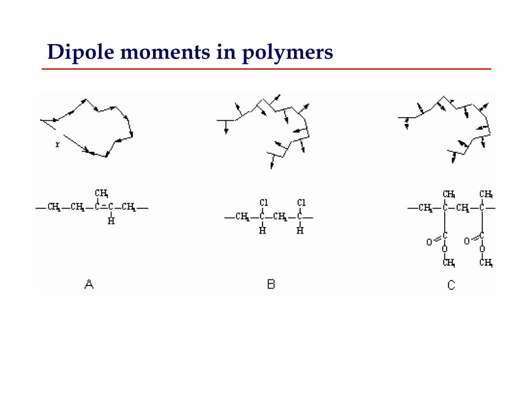
Dipole moments in polymers

Molecular motions accommodate dipole reorientation in polymers

Decreasing frequency of external field

Dielectric dispersion in frequency domain

10-1

100

101

102

103

104

105

10-1

100

d

iele

ctr

ic lo

ss

, εε εε'

'

frequency [Hz]

- 60°C - 40°C

- 120°C

- 90°C

10-1

2x10-1

3x10-1

�, � relaxations

Depends on chemical structure and local molecular environment

• Motion of groups present in side chain around

the main chain or bonds of the side chain

• Motion of groups in the main chain

• The � relaxation of Johari-Goldstein type

Glassy state (localized motions) I

Thermally activated motion

between two potential wells

separated by a potential barrier

• Temperature dependence of relaxation rate (time) is Arrhenius

• Dielectric strength, ��, increases with increasing T, more dipoles contribute

• Broad (4-6 decades) symmetric dielectric dispersion, becomes narrower with increasing T as a result of molecular environment homogenization

Glassy state (localized motions) II

Characteristics of dielectric dispersion

−= ∞kT

Eff actexpββ

V

N

kTgFOnsager

2µε ∝∆

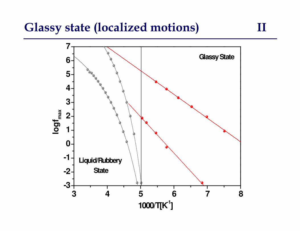
Glassy state (localized motions) II

3 4 5 6 7 8-3

-2

-1

0

1

2

3

4

5

6

7

Liquid/Rubbery

State

log

f max

1000/T[K-1]

Glassy State

� relaxation (dynamic glass transition)

• relaxation time reflects the time involved in the structural rearrangement (glass transition) of the molecules

• ττττ changes by many orders of magnitude from the liquid to the glass

• The αααα-relaxation in polymers involves cooperative micro-Brownian

segmental motions of the chains

• Segmental motions are associated with conformational transitions

taking place about the skeletal bonds

Rubbery/liquid state (segmental motions) I

Rubbery/liquid state (segmental motions) II

• Temperature dependence of relaxation rate (time) described by VTF equation

• Dielectric strength, ��, decreases with increasing T more strongly than predicted by

• Asymmetric dielectric dispersion

• High f side slope, n: local chain dynamics (n increases as T increases)

• Low f side slope, m: cooperative dynamics of environment (m increases as T increases)

Characteristics of dielectric dispersion

−−= ∞

0

expTT

Bff αα

V

N

kTgFOnsager

2µε ∝∆

3 4 5 6 7 8-3

-2

-1

0

1

2

3

4

5

6

7

Liquid/Rubbery

State

log

f max

1000/T[K-1]

Glassy State

Rubbery/liquid state (global motions) I

• Observed in polymers containing dipoles type A and AB

• Motions of the whole chain

• Observed at frequencies lower than the αααα relaxation

• The relaxation time of the process is strongly

dependent of the molecular weight

Rubbery/liquid state (global motions) I

Normal mode relaxation (nm)

• T dependence of relaxation rate (time)

same as this of � relaxation

• Dielectric strength proportional to the

mean end-to-end vector of chain

• m=1 and n=0.7 predicted by theory, in practice n considerably smaller

Rubbery/liquid state (global motions) II

Characteristics of dielectric dispersion

2

2

3

4r

kTM

FN OnsagerpA

nm

µπε =∆

3 4 5 6 7 8-3

-2

-1

0

1

2

3

4

5

6

7

Liquid/Rubbery

State

log

f max

1000/T[K-1]

Glassy State

• Motion of charge carriers

• �’ is not affected

• �’’ increases with decreasing f (slope of log�’’vs logf equal to -1)

• �’ independent of f equal to dc conductivity, �dc

• T dependence of �dcArrhenius, VTF or other gives information on the conductivity mechanism

Rubbery/liquid state (charge motions)

Conductivity

( ) ( ) ( ) ( )( )1*

0

* −=′′+′= ωεωεωσωσωσ ii

( ) ( )ωεωεωσ ′′=′0

( ) ( )( )10 −′=′′ ωεωεωσ

• Blocking of charges at interfaces inside inhomogeneous materials

• Existence of regions with different characteristics (�, �)• Relaxation rate (time) depends on:

volume fraction, shape, � and � values of regions

Separation of charges at interfaces

Maxwell-Wagner-Sillars relaxation (MWS)

Electrode Polarization

• Blocking of charges at sample/electrode interfaces

• Observed as a steep increase of �’• Magnitude and frequency position of the process depend on the conductivity of

the sample (high values of � shift polarization to high f)• Time of the process depends on the sample thickness (increase of thickness

results in an increase of time of process)

Comparison with other techniques

• Understanding the correlation between parameters of the molecular and supermolecular structures and macroscopic properties.

• Contribution to open questions regarding the � relaxation bycovering the widest possible time/frequency scale range by different experimental techniques

Material testing method & tool for studying dynamics in polymers

• Material in an external mechanical field

• insulator�elastic solid, conductor�viscous liquid

• Viscoelastic response is analogous to dielectric dispersion

• Modulus representation is used

• In order dielectric dispersion be compared to mechanical one electric modulus has to be used for data representation

Comparison with Mechanical measurements

( )( )ωε

ω*

* 1=M

Comparison with Mechanical measurements

Extension in broad f range by constructing master plots

Comparison with Mechanical measurements

Comparison of relaxation time temperature dependence

Comparison with Mechanical measurements

Selectivity of dielectric spectroscopy (block copolymers)

• Observation of the dynamics on a microscopic length and time scale

(10-7-10-11s)

• S(Q, �) contains not only temporal information but also spatial information of the particle correlation function

Comparison with Quasielastic Neutron Scattering

Comparison with Quasielastic Neutron Scattering

Different T Different T

Comparison with Quasielastic Neutron Scattering

( ) ( ) ( )QTTQ τατ =,

( )TAQ ,11−°=τ

( )Tdielτ

Comparable to

( ) ( )( )ωω

ω *Im1

, Φ−=QS

References

A. Broadband dielectric spectroscopy, F. Kremer and A. Schoenhals eds.Chapter 1Theory of Dielectric Relaxation A. Schoenhals and F. KremerChapter 7Molecular dynamics in polymer model systems, A. SchoenhalsChapter 16Dielectric and Mechanical Spectroscopy a Comparison, T. PakulaChapter 18Polymer dynamics by dielectric spectroscopy and neutron scattering-a comparison,A. Arbe, J. Colmenero and D. Richter

B. Electrical Properties of Polymers, E. Riande and R. Diaz-Calleja

C. Dielectric Spectroscopy of Polymeric materials, J. Runt and J. Fitzgerald