dielectric constant of the polarizable dipolar hard sphere

Condensed Matter Physics, 2005, Vol. 8, No. 2(42), pp. 357–376

Dielectric constant of the polarizabledipolar hard sphere fluid studied byMonte Carlo simulation and theories

M.Valisko, D.Boda

Department of Physical Chemistry,University of Veszprem,H–8201 Veszprem, PO Box 158, Hungary

Received October 29, 2004

A systematic Monte Carlo (MC) simulation and perturbation theoretical(PT) study is reported for the dielectric constant of the polarizable dipo-lar hard sphere (PDHS) fluid. We take the polarizability of the moleculesinto account in two different ways. In a continuum approach we place thepermanent dipole of the molecule into a sphere of dielectric constant ε∞

in the spirit of Onsager. The high frequency dielectric constant ε∞ is cal-culated from the Clausius-Mosotti relation, while the dielectric constant ofthe polarizable fluid is obtained from the Kirkwood-Frohlich equation. In themolecular approach, the polarizability is built into the model on the molec-ular level, which makes the interactions non- pairwise additive. Here weuse Wertheim’s renormalized PT method to calculate the induced dipolemoment, while the dielectric constant is calculated from our recently in-troduced formula [22]. We also apply a series expansion for the dielectricconstant both in the continuum and the molecular approach. These seriesexpansions ensure a better agreement with simulation results. The agree-ment between our MC data and the PT results in the molecular approachis excellent for low to moderate dipole moments and polarizabilities. Atstronger dipolar interactions ergodicity problems and anizotropic behaviourappear where simulation results become uncertain and the theoretical ap-proach becomes invalid.

Key words: dielectric constant, Monte Carlo, polarizable fluids

PACS: 61.20.Gy, 61.20.Ja, 61.20.Ne

1. Introduction

The classical theories of the dielectric constant founded by Kirkwood [1], On-sager [2], and Debye [3] use a continuum approach: they place the molecule in acavity surrounded by the material treated as a continuum. The Clausius-Mosotti(CM) equation is valid for apolar molecules, while the Debye equation [3] holds

c© M.Valisko, D.Boda 357

M.Valisko, D.Boda

good approximately to gases and dilute solutions of molecules carrying a permanentdipole. The Debye equation for a spherical shaped sample is:

ε − 1

ε + 2=

4π

3αρ + y0 , (1)

where α is the polarizability of the molecule, ρ = N/V is the number density, andy0 is the dimensionless dipole strength function, y0 = 4πρµ2

0/9kT , where µ0 is thepermanent dipole moment, k is the Boltzmann factor and T is the temperature (forµ0 = 0, equation (1) yields the CM equation). Onsager [2] placed a point dipolein the centre of a cavity of dielectric constant ε∞ and the effect of the surroundingdielectric is measured by the dielectric response of the polarization charges inducedon the wall of the cavity. The resulting equation is

(ε − ε∞) (2ε + ε∞)

ε (ε∞ + 2)2= y0, (2)

where ε∞ is the high frequency dielectric constant, which is related to the molecularpolarizability via the CM equation

ε∞ − 1

ε∞ + 2=

4π

3αρ . (3)

The Onsager equation works quite well for liquids when the dipole moment is nottoo high.

When the molecules have a large permanent dipole moment, the correlationbetween a central dipole and the surrounding dipoles cannot be replaced by theresponse of a continuum dielectric. Kirkwood has introduced the so-called Kirkwoodg-factor to take into account these short range correlations. The g-factor is obtainedfrom the fluctuation of the total dipole moment of the system M,

gK =〈M2〉

Nµ20

, (4)

where 〈· · ·〉 denotes ensemble average. For a liquid consisting of non-polarizablemolecules, the Kirkwood-equation reads as

(ε − 1)(2ε + 1)

9ε= y0gK . (5)

To take into account the molecular polarizability, we can choose the continuum ap-

proach used by Onsager. In this case we obtain the Kirkwood-Frohlich (KF) equa-tion [4]

(ε − ε∞)(2ε + ε∞)

ε(ε∞ + 2)2= y0gK . (6)

It is seen that the difference between this equation and the Osager equation, (2), isthat the Kirkwood factor is present on the right hand side representing the corre-lation between the permanent dipoles of the molecules. Nevertheless, this is still a

358

Dielectric constant of the PDHS fluid

continuum theory regarding polarizability, and y0 is calculated by using the perma-nent dipole moment µ0 (that is why the subscript 0 is used).

When a molecular polarizability is added to the permanent dipole of a dipolarmolecule, we take into account the polarizability on the molecular level: we call thisthe molecular approach. The equation that applies for this case is

(ε − 1)(2ε + 1)

9ε=

4π

3αρ + ygK. (7)

In this equation y is calculated by using the total (permanent plus induced) dipolemoment of the molecules (subsript 0 is absent) and gK contains the correlationbetween permanent and induced dipoles too.

To calculate gK, a molecular model and a statistical mechanical method areneeded to study it. In the case of the Kirkwood, (5) and the KF, (6), equations, thecalculation of gK is relatively simple because the pair-wise additive dipole-dipole in-teraction is considered and the calculation of pair correlation functions is sufficient.Nevertheless, when the molecular polarizability is included in the model, the inter-molecular potential is no longer pairwise additive and many-body correlations haveto be taken into account. This is the characteristic problem that greatly complicatesthe statistical mechanical treatment of the systems containing strongly interactingpolarizable dipoles.

Most theories rather avoid the treatment of these many-body correlations bymimicing the polarizable fluid with a system characterized by a pairwise addi-tive interaction applying an effective permanent dipole moment. This approach wasused by the graph-theoretical treatment of Wertheim [5], its extension to dipolar-quadrupolar fluids and mixtures [6–8], and a self consistent mean field (SCMF)approach of Carnie and Patey [9]. In these approaches, a theory is needed to cal-culate the properties of the system defined by the effective pair potential. For thispurpose, one can use the hypernetted chain theories [9,10] or the thermodynamicperturbation theory (PT) which was developed by many authors during the sec-ond half of the twentieth century [11–21]. A major breakthrough was the theory ofBarker and Henderson [13–17] which was the first useful PT. The PT was used inour previous paper [22] where we proposed an equation for the dielectric constantof polarizable polar fluids. We use this equation to study the dielectric constant ofthe polarizable dipolar hard sphere (PDHS) fluid in this work.

In computer simulations, the treatment of non-additive potentials is straightfor-ward since the pioneering works by Vesely [23,24]. The problem here lies in the timeconsuming iteration procedure calculating the induced dipoles in every simulationstep. After a few early works [10,23–27], more and more computer simulation studi-es of polarizable fluids have been appearing in the literature due to the continouslyincreasing speed of computers [28–35]. While the earlier works dealt with simplermodels such as PDHS or polarizable Stockmayer (PSTM) fluids, the latter worksconcentrated on more complex molecular liquid models aimed at representing realsubstances, first of all, water. Lately, the authors seem to have lost interest in sim-ple potential models. This is probably due to the increasing power of computers.

359

M.Valisko, D.Boda

Thus computer simulation became an everyday tool and investigators are capableof studying more and more sophisticated models for a specific material. Neverthe-less, this specification results in a loss of generality meaning that simple models cancapture a few important, characteristic features of a whole class of systems, whiledetailed models are restricted to the molecule for which they have been designed.

Notable exceptions in this trend of specification are the works of Kriebel andWinkelmann [36,37] who gave a systematic study of the thermodynamic propertiesof the PSTM [36] and the polarizable dipolar two-centred Lennard-Jones (LJ) fluid[37]. Nevertheless, they did not have interest in the dielectric properties of thesesystems. In an earlier work [38], we studied the dielectric constant of this systemusing Monte Carlo (MC) simulaton and our renormalized PT equation proposedpreviously [22].

The PDHS model, which we consider in this work, is probably the simplestmolecular model for a polarizable dipolar fluid. The core is a hard sphere (HS)which gives the molecules finite size, so contributions from excluded volume effectscan be studied. Using this simple model for the core, we can concentrate on theeffect of electrostatic interactions. In this study, we use both the continuum ap-

proach (equation (6)) and the molecular approach (equation (7)) to calculate thedielectric constant of the PDHS fluid over a wide range of density, dipole moment,and polarizability. The results obtained from the theories are compared to our ownMC simulation data that are obtained using the pair approximation of polarizationinteraction (PAPI) method of Predota et al. [35] in order to accelerate calculations.

It is known since the work of Tani et al. [39] for the dipolar hard sphere (DHS)fluid that equation (5) gives poor results in the liquid phase for the dielectric constantof the DHS fluid using PT to calculate gK compared to simulation data. Nevertheless,if we expand ε(y0) into a Taylor series as a function of the dipole strength functiony0, we obtain much more reasonable results. We detail the nature and importance ofthis series expansion in subsequent sections and we develop such series expanions forthe case of polarizable fluids using both the continuum and the molecular approach.We will show that these series expansions give results in better agreement with MCdata than the original equations, (6) and (7) do.

2. Models

First, we introduce the PDHS model, of which the DHS fluid is a special case withα = 0. Since the potential in the PDHS system is not pair-wise additive, we have todefine the total energy of the system for a complete definition of the Hamiltonian.In the case of the DHS fluid, of course, the system can be defined merely by givingthe pair potential; the total energy is the sum of the pair potentials.

The total energy of the N -particle system of the PDHS fluid can be divided intothree parts:

U = Uref + Uel + Uind . (8)

The first part, the non-electrostatic spherical reference potential is a sum of pair-wise

360


additive potentials which is the HS potential in this study:

uHS(rij) =

{

∞ if rij < σ0 if rij > σ

, (9)

where σ is the hard sphere diameter and rij is the magnitude of the vector rij =ri − rj . This term merely forbids the overlapping of the spheres. The electrostaticterms of the energy consist of the interaction between the permanent dipoles

Uel = −1

2

∑

i

(µ0)i (E0)i (10)

and the induction energy [31]

Uind = −1

2

∑

i

(µind)i (E0)i , (11)

where (µ0)i and (µind)i are the permanent and the induced dipole moments on thei-th molecule, respectively, and (E0)i is the electric field raised at the place of thei-th molecule by the permanent dipoles of all other molecules:

(E0)i = −∑

j 6=i

Tij (µ0)j (12)

with

Tij =

(

δij

r3ij

−3rijrij

r5ij

)

(13)

being the electrostatic tensor. Introducing the electric field raised at the place ofmolecule i by the induced dipoles of all other molecules

(Eind)i = −∑

j 6=i

Tij (µind)j , (14)

the induced dipole moment of the i-th molecule can be written as

(µind)i = α [(E0)i+ (Eind)i

] . (15)

In general, α is a tensor, but in this study, we restrict ourselves to a scalar polar-izability. For the non-polarizable case Uind = 0, and Uel reduces to the sum of thedipole-dipole pair potentials

uDD(ij) = −µ20

(

3(nirij)(njrij)

r5ij

−ninj

r3ij

)

, (16)

where (ij) is a notation for (rij,ni,nj) and ni = µi/µ0 is the unit vector in thedirection of the i-th dipole.

361

M.Valisko, D.Boda

3. Monte Carlo simulations

Computer simulations provide an efficient method to study many-particle ther-modynamic systems. For a well defined system, the results of simulations are accept-ed as a gold standard to which the results of various theories, which usually containsome approximation, can be compared. By well defined system we mean that theinteraction potential acting between the particles together with a few thermodynam-ic parameters that define the thermodynamic state are given. The details of bothMC and molecular dynamics simulations are given in excellent books [40–42], herewe only describe some aspects regarding the calculation of induced dipoles and thedielectric constant.

Normally, in an MC step only one molecule is displaced. In the case of the non-additive polarizable dipole potential a self consistent iteration procedure based onequations (14) and (15) is needed to calculate (µind)i for a given configuration. Thevalues of the induced dipoles are needed to calculate the energy from equations (10)and (11). The computer time cost of the iteration procedure is proportional to N2.Therefore, MC simulation seems to be a less economic method for non-additivepotentials if single particle moves and full iteration are used.

To decrease computational burden of MC simulations, Predota et al. [35] havesuggested a procedure called “pair approximation for polarization interaction” (PA-PI). The basis of their idea is that after a small displacement of a single particle, afull update of the induced dipoles is necessary only in the close neighbourhood ofthe displaced molecule i, namely, close to the source of the disturbance that causesthe reordering of the induced dipoles. The neighbourhood for which full iteration isperformed is defined as two spheres around the old and the new position of moleculei with a radius Riter. The change of the induced dipole moment in an iteration iscalculated from

∆(µind)j = α [∆(Eind)j + ∆(E0)j] , (17)

where the change of the induced electric field in the iteration is given by

∆(E ind)j =

∆(Eind)ij +∑

j′ ∆(E ind)ij′ , if j ∈ Riter ,

j′ 6=i,j; j′∈Riter

∆(Eind)ij , otherwise.(18)

This means that the interactions between the displaced molecule i and an arbitrarymolecule j are always taken into account in the calculation of ∆(Eind)j . Furthermore,all interactions between pairs of molecules j, j′ that are within the cutoff spheresare also taken into account, while interactions between pairs where one of the twomolecules is outside the spheres are ignored. The change of the electric field producedby the permanent dipoles, ∆(E0)j , is nonzero only in the first iteration.

The dielectric constant can be determined from the following formula [26,31]

(ε − 1)(2εRF + 1)

3(2εRF + ε)=

(ε∞ − 1)(2εRF + 1)

3(2εRF + ε∞)+

4πρ

9kT

⟨

M 2⟩

N. (19)

362


This equation assumes that a spherical sample of polar molecules is surrounded by auniform dielectric of dielectric constant εRF. The notation RF refers to the reactionfield produced by the polarization charges induced on the boundary of the sampleand the surrounding dielectric. The high frequency dielectric constant, ε∞, can becalculated from the CM relationship (equation (3)). Nevertheless, replacing the firstterm on the right hand side by 4παρ/3 practically yields the same result for ε. Theabove formulation for the dielectric constant has to be consistent with the energycalculation in the simulations, namely, the term

−2(εRF − 1)

2εRF + 1

δij

R3c

(20)

has to be added to the dielectric tensor in equation (13), where Rc is the cutoff radiusof the dipolar interactions (taken to be equal to the half of the width of the simulationbox, L/2). Without using any summation technique to estimate contributions ofperiodic images to the potential (such as the Ewald technique), this procedure isthe so-called reaction field method to treat long range corrections [43]. In this work,the tin-foil or conducting boundary condition (εRF → ∞) was used.

The number of particles was 256 for most cases, 108 particles were used in a fewcases for low density (ρ∗ = ρσ3 = 0.2), and a few simulations have been performedwith 512 and 1000 particles for comparison. The lengths of the simulations variedbetween 100 and 500 thousand MC cycles depending on the dipolar strengths anddensity (longer runs were used for higher densities and higher dipole moments). Inan MC cycle N attempts were made to move a particle. In an MC movement, themolecule was attempted to be displaced and rotated randomly with respect to itsold coordinates. The maximum displacements had to be kept at low values in orderto maintain a fast convergence in the calculation of the induced dipoles in the PAPIprocedure. The radius Riter of the PAPI technique was set to 2.5σ for higher densities(ρ∗ = 0.6 and 0.8) and 3σ for lower densities (ρ∗ = 0.2 and 0.4). A full iteration wasmade in every tenth MC cycle. The statistical errors were estimated from the blockaverage method.

4. Theories

There are two basic problems that we expect from our theories to provide solutionfor. The first problem is the calculation of the Kirkwood factor for a dipolar fluid.The thermodynamic PT that determines it for the non-polarizable DHS fluid isdescribed in the next subsection. The other problem is the consideration of themolecular polarizability. A continuum and a molecular approach, already looselydesribed in the Introduction, are presented in the subsequent subsections.

4.1. Non-polarizable case

To calculate the dielectric constant of the DHS fluid, the starting point is theKirkwood equation, (5). The Kirkwood g-factor (equation (4)) takes care of the short

363

M.Valisko, D.Boda

range correlations between the dipoles. It can be related to the ensemble average ofthe function ∆(1j) = n1 · nj by

gK = 1 +

⟨

N∑

j=2

∆(1j)

⟩

= 1 +

∫

〈g(12)∆(12)〉ω1ω2dr12 , (21)

where 〈· · ·〉 denotes ensemble average which can be determined using the pair-correlation function g(12). The notation 〈· · ·〉ω1ω2

means averaging over orientations.Perturbation theories [11–21] divide the intermolecular potential into an isotropicreference state and a perturbation part (uHS is the reference potential and uDD isthe perturbation term). For the pair correlation function of the DHS system theperturbation series expansion read as

g(12) = g0(12) − βuDD(12)g0(12) + β2ρ

∫

〈uDD(13)uDD(23)〉ω3g0(123)dr3 , (22)

where g0(12) and g0(123) are the two- and the three-particle correlation functionsof the reference (HS) system, respectively, and β = 1/kT . The three-particle distri-bution function has been calculated by the Kirkwood superposition approximation:g0(123) = g0(12)g0(23)g0(13) as suggested by Barker et al. [15–17]. Performing theangular integrals and using orthogonality relations the Kirkwood factor can be ex-pressed as [39,44–47]

gK = 1 + y20

9Idd∆

16π2, (23)

where Idd∆ denotes a triple integral that can be given as

Idd∆ =

∫

3 cos2 θ3 − 1

(r13r23)3g0(123)dr2dr3 , (24)

where θ3 is the interior angle of the (123) triangle. For the DHS fluid, the valuesof the integral depend only on the dimensionless reduced density ρ∗ = ρσ3 throughg0(123). The ρ∗-dependence can be given by the following polynomial:

Idd∆(ρ∗) = 18.6426−0.0352ρ∗+2.2950ρ∗2+2.9831ρ∗3−0.0665ρ∗4+2.3666ρ∗5 . (25)

This expansion was obtained by a fit to values that we calculated with the Fouriertransform convolution theorem [47] and it provides results that are virtually identicalto those given by the Pade type expression reported by Tani et al. (equation (17) in[39]). Substituting equation (23) into equation (5), the Kirkwood equation can berewritten as

(ε − 1)(2ε + 1)

9ε= y0

(

1 + y20

9Idd∆

16π2

)

. (DHS1) (26)

The results calculated from equation (26) are not in good agreement with the sim-ulation data, so Tani et al. [39] expanded ε(y0) as a Taylor series on the basis of theabove equation and obtained that

ε(y0) = 1 + 3y0 + 3y20 + 3y3

0

(

9Idd∆

16π2− 1

)

+ · · · (DHS2) (27)

364


Tani et al. have shown that the results from the above series expansion of the Kirk-wood equation is in better agreement with the simulation data than those calculatedfrom the Kirkwood equation itself, (26). Goldman [47] has found the same for theStockmayer fluid. These series expansions, apart from the fact that they give betteragreement with simulation results, have a strong theoretical basis. Jepsen [48,49]and Rushbrook [45,50] have shown for the DHS fluid that the next exact term inthe y0-expansion of the Debye equation is

ε − 1

ε + 2= y0 −

15

16y2

0 (28)

from which the following series can be derived for the dielectric constant:

ε = 1 + 3y0 + 3y20 +

3

16y3

0 + · · · (29)

This equation is exact in the limit of low densities. The Onsager [2] and the vanVleck [51] theories are valid up to the second order in y0. The y0-expansion of thedielectric constant given by Wertheim’s MSA method [52] yields this equation too.Note that in the low density limit Idd∆ = 17π2/9 and equation (27) becomes identicalto equation (29).

These considerations support that such a series expansion is not merely a com-putational trick but it is an equation that is independent of the boundary conditionsand the shape of the sample. Equations written in a form of the Kirkwood, the On-sager, or the CM equations explicitly include the information about the boundaryconditions (left hand side of the equations). Accordingly, the Kirkwood factor onthe right hand side of the equations will also depend on the boundary conditions be-cause the resulting dielectric constant should be independent of them. Nevertheless,in theory the bulk system is considered as infinite and the Idd∆ integral includesinformation only on the short range correlations of a central dipole and its localenvironment and knows nothing about boundary condition of the macroscopic sam-ple. Therefore, it is reasonable to express the dielectric constant in a form that isindependent of boundary conditions.

It is important to note that equation (27) can be obtained using a different route.Szalai et al. [53] studied the DHS fluid in the presence of an external electric field.Assuming that the shape of the sample is an infinitely prolate ellipsoid (which meansthe field inside the dielectric equals the external field), they have expressed the fielddependent Helmholtz free energy of the system, F (E0). The relation between thepolarization and the free energy is

P = −1

V

(

∂F (E0)

∂E0

)

NV T

, (30)

from which the dielectric constant follows. The resulting equation for ε is the sameas equation (27). The approach based on the response to an external field can beapplied within the framework of the MSA [54,55] and for the calculation of themagnetic susceptibility of magnetic fluids using simulations [56–59].

365

M.Valisko, D.Boda

4.2. The continuum approach

In the above section the polarizability α of the molecules was not taken into ac-count. In our previous works [60,61] we have proposed a simple continuum approach

based on the KF equation, (6). If we express the Kirkwood factor using the aboveoutlined PT approach, we obtain the following equation

(ε − ε∞)(2ε + ε∞)

ε(ε∞ + 2)2= y0

(

1 + y20

9Idd∆

16π2

)

. (KF1) (31)

The high frequency dielectric constant can be obtained from the CM equation (3).Following the reasoning given in the previous section, we can assume that the seriesexpansion of the above equation might also give a more general equation for thedielectric constant. Performing the same series expansion for the KF equation asTani et al. [39] did for the Kirkwood equation, we obtain [60] that

ε(y0) = ε∞ +ε∞(ε∞ + 2)2

2ε∞ + 1y0 +

ε∞(ε∞ + 2)4

(2ε∞ + 1)3y2

0

+ε∞(ε∞ + 2)2

2ε∞ + 1

[

9Idd∆

16π2−

(2ε∞ − 1)(ε∞ + 2)4

(2ε∞ + 1)4

]

y30 . (KF2) (32)

Note that with ε∞ = 1 equation (32) yields equation (27).

4.3. The molecular approach

If we want to treat the molecular polarizability in a self consistent way on themolecular level, we have to use a theory that is capable of treating the non-additivemany-body interactions. Wertheim [5] developed a graph-theory in which a renor-malized effective dipole moment µ is defined as a sum of the permanent dipolemoment µ0 and the induced dipole moment resulting from the mean electric field Eacting on the molecules:

µ = µ0 + αE . (33)

Gray et al. [6–8] showed that the mean electric field can be given as:

E = −

(

∂f

∂µ

)

αV T

, (34)

where f is the one-particle Helmholtz free energy of the system. The above twoequations provide a self consistent iteration route that can be solved for the effec-tive dipole moment. For the free energy, a Pade approximant can be given with freeenergy perturbation terms that can be calculated if one knows the g0 radial distri-bution function of the reference HS system. The exact forms of these perturbationintegrals can be found elsewhere [21,36].

After the renormalization iteration procedure we obtain the effective dipole mo-ment as a function of α and µ0. Equation (7) is used as a starting point for the

366


calculation of the dielectric constant. In our previous work [22], we have given anexpression for ygK:

ygK =4πµ2

9kTρ +

4π

3Idd∆

[

(

µ2

3kT+ α

)3

− α3

]

ρ3 . (35)

Introducing the parameters

a =4π

3

(

µ2

3kT+ α

)

(36)

and

b =4π

3Idd∆

[

(

µ2

3kT+ α

)3

− α3

]

, (37)

equation (7) can be expressed as

(ε − 1)(2ε + 1)

9ε= aρ + bρ3. (PDHS1) (38)

0

10

20

30

40

50

ε

MCPDHS1KF1DHS1PDHS2KF2DHS2

0

30

60

90

120

150

ε

0 0.2 0.4 0.6 0.8ρ*

0

15

30

45

60

ε

0.2 0.4 0.6 0.8ρ*

0

5

10

15

20

ε

α∗=0.02, (µ0*)

2=3.0

α∗=0.06, (µ0*)

2=1.0α∗=0.04, (µ

0*)

2=2.0

α∗=0.02, (µ0*)

2=2.0

(a) (b)

(d)(c)

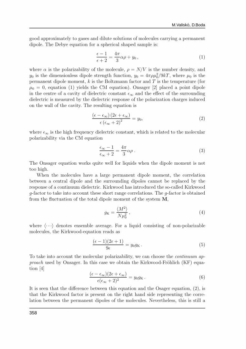
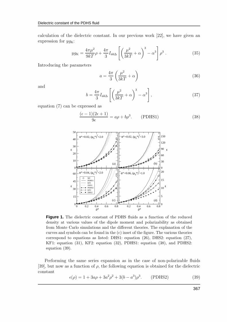
Figure 1. The dielectric constant of PDHS fluids as a function of the reduceddensity at various values of the dipole moment and polarizability as obtainedfrom Monte Carlo simulations and the different theories. The explanation of thecurves and symbols can be found in the (c) inset of the figure. The various theoriescorrespond to equations as listed: DHS1: equation (26), DHS2: equation (27),KF1: equation (31), KF2: equation (32), PDHS1: equation (38), and PDHS2:equation (39).

Performing the same series expansion as in the case of non-polarizable fluids[39], but now as a function of ρ, the following equation is obtained for the dielectricconstant

ε(ρ) = 1 + 3aρ + 3a2ρ2 + 3(b − a3)ρ3. (PDHS2) (39)

367

M.Valisko, D.Boda

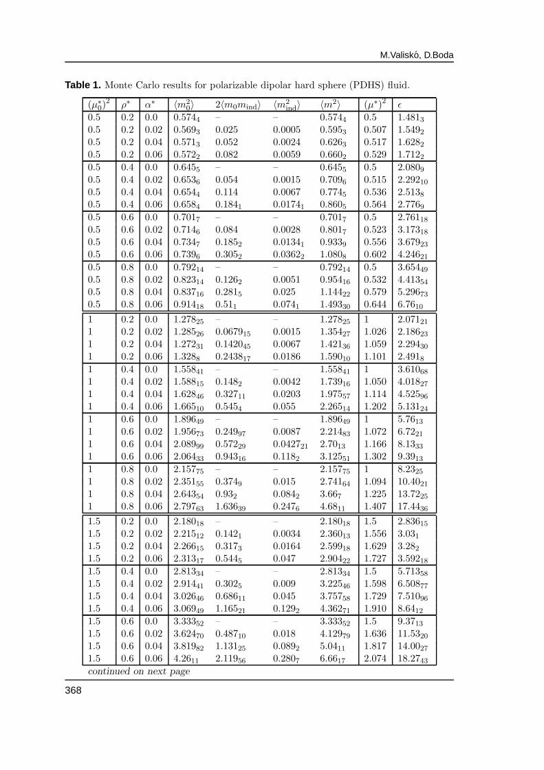
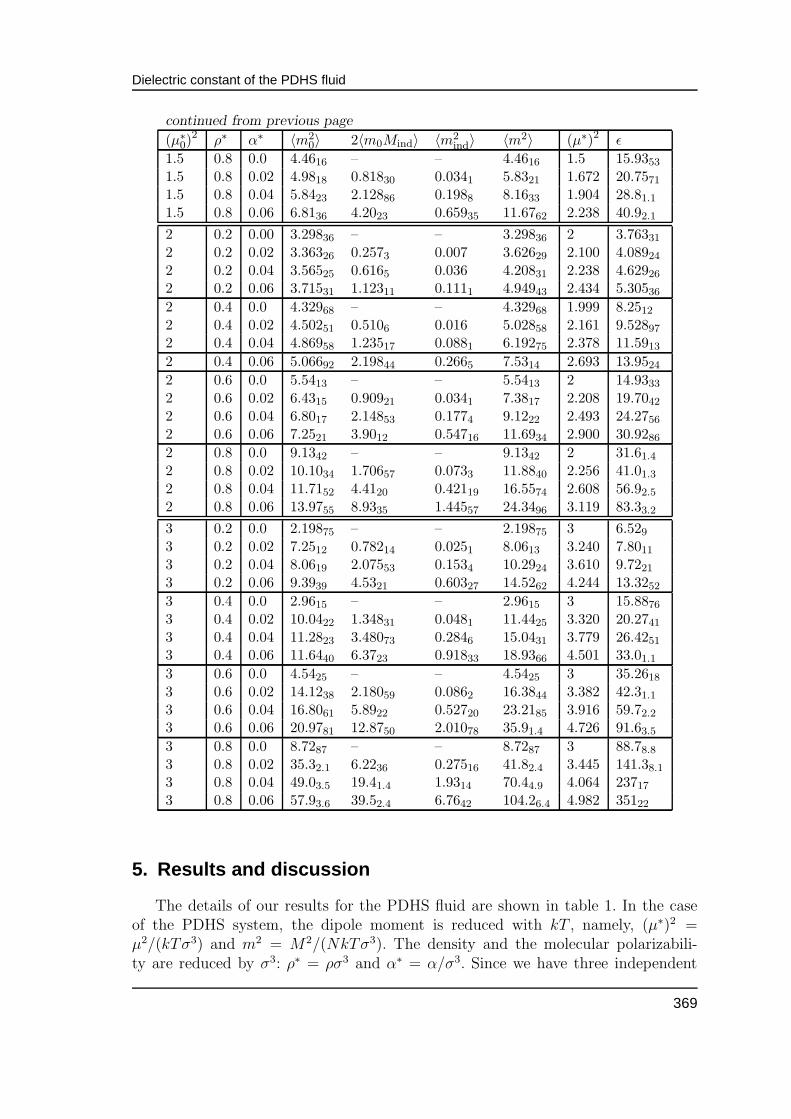
Table 1. Monte Carlo results for polarizable dipolar hard sphere (PDHS) fluid.

(µ∗0)

2ρ∗ α∗ 〈m2

0〉 2〈m0mind〉〈m2ind〉〈m2〉 (µ∗)2 ε

0.5 0.2 0.0 0.5744 – – 0.5744 0.5 1.4813

0.5 0.2 0.02 0.5693 0.025 0.0005 0.5953 0.507 1.5492

0.5 0.2 0.04 0.5713 0.052 0.0024 0.6263 0.517 1.6282

0.5 0.2 0.06 0.5722 0.082 0.0059 0.6602 0.529 1.7122

0.5 0.4 0.0 0.6455 – – 0.6455 0.5 2.0809

0.5 0.4 0.02 0.6536 0.054 0.0015 0.7096 0.515 2.29210

0.5 0.4 0.04 0.6544 0.114 0.0067 0.7745 0.536 2.5138

0.5 0.4 0.06 0.6584 0.1841 0.01741 0.8605 0.564 2.7769

0.5 0.6 0.0 0.7017 – – 0.7017 0.5 2.76118

0.5 0.6 0.02 0.7146 0.084 0.0028 0.8017 0.523 3.17318

0.5 0.6 0.04 0.7347 0.1852 0.01341 0.9339 0.556 3.67923

0.5 0.6 0.06 0.7396 0.3052 0.03622 1.0808 0.602 4.24621

0.5 0.8 0.0 0.79214 – – 0.79214 0.5 3.65449

0.5 0.8 0.02 0.82314 0.1262 0.0051 0.95416 0.532 4.41354

0.5 0.8 0.04 0.83716 0.2815 0.025 1.14422 0.579 5.29673

0.5 0.8 0.06 0.91418 0.511 0.0741 1.49330 0.644 6.7610

1 0.2 0.0 1.27825 – – 1.27825 1 2.07121

1 0.2 0.02 1.28526 0.067915 0.0015 1.35427 1.026 2.18623

1 0.2 0.04 1.27231 0.142045 0.0067 1.42136 1.059 2.29430

1 0.2 0.06 1.3288 0.243817 0.0186 1.59010 1.101 2.4918

1 0.4 0.0 1.55841 – – 1.55841 1 3.61068

1 0.4 0.02 1.58815 0.1482 0.0042 1.73916 1.050 4.01827

1 0.4 0.04 1.62846 0.32711 0.0203 1.97557 1.114 4.52596

1 0.4 0.06 1.66510 0.5454 0.055 2.26514 1.202 5.13124

1 0.6 0.0 1.89649 – – 1.89649 1 5.7613

1 0.6 0.02 1.95673 0.24997 0.0087 2.21483 1.072 6.7221

1 0.6 0.04 2.08999 0.57229 0.042721 2.7013 1.166 8.1333

1 0.6 0.06 2.06433 0.94316 0.1182 3.12551 1.302 9.3913

1 0.8 0.0 2.15775 – – 2.15775 1 8.2325

1 0.8 0.02 2.35155 0.3749 0.015 2.74164 1.094 10.4021

1 0.8 0.04 2.64354 0.932 0.0842 3.667 1.225 13.7225

1 0.8 0.06 2.79763 1.63639 0.2476 4.6811 1.407 17.4436

1.5 0.2 0.0 2.18018 – – 2.18018 1.5 2.83615

1.5 0.2 0.02 2.21512 0.1421 0.0034 2.36013 1.556 3.031

1.5 0.2 0.04 2.26615 0.3173 0.0164 2.59918 1.629 3.282

1.5 0.2 0.06 2.31317 0.5445 0.047 2.90422 1.727 3.59218

1.5 0.4 0.0 2.81334 – – 2.81334 1.5 5.71358

1.5 0.4 0.02 2.91441 0.3025 0.009 3.22546 1.598 6.50877

1.5 0.4 0.04 3.02646 0.68611 0.045 3.75758 1.729 7.51096

1.5 0.4 0.06 3.06949 1.16521 0.1292 4.36271 1.910 8.6412

1.5 0.6 0.0 3.33352 – – 3.33352 1.5 9.3713

1.5 0.6 0.02 3.62470 0.48710 0.018 4.12979 1.636 11.5320

1.5 0.6 0.04 3.81982 1.13125 0.0892 5.0411 1.817 14.0027

1.5 0.6 0.06 4.2611 2.11956 0.2807 6.6617 2.074 18.2743

continued on next page

368


continued from previous page

(µ∗0)

2ρ∗ α∗ 〈m2

0〉 2〈m0Mind〉〈m2ind〉〈m2〉 (µ∗)2 ε

1.5 0.8 0.0 4.4616 – – 4.4616 1.5 15.9353

1.5 0.8 0.02 4.9818 0.81830 0.0341 5.8321 1.672 20.7571

1.5 0.8 0.04 5.8423 2.12886 0.1988 8.1633 1.904 28.81.1

1.5 0.8 0.06 6.8136 4.2023 0.65935 11.6762 2.238 40.92.1

2 0.2 0.00 3.29836 – – 3.29836 2 3.76331

2 0.2 0.02 3.36326 0.2573 0.007 3.62629 2.100 4.08924

2 0.2 0.04 3.56525 0.6165 0.036 4.20831 2.238 4.62926

2 0.2 0.06 3.71531 1.12311 0.1111 4.94943 2.434 5.30536

2 0.4 0.0 4.32968 – – 4.32968 1.999 8.2512

2 0.4 0.02 4.50251 0.5106 0.016 5.02858 2.161 9.52897

2 0.4 0.04 4.86958 1.23517 0.0881 6.19275 2.378 11.5913

2 0.4 0.06 5.06692 2.19844 0.2665 7.5314 2.693 13.9524

2 0.6 0.0 5.5413 – – 5.5413 2 14.9333

2 0.6 0.02 6.4315 0.90921 0.0341 7.3817 2.208 19.7042

2 0.6 0.04 6.8017 2.14853 0.1774 9.1222 2.493 24.2756

2 0.6 0.06 7.2521 3.9012 0.54716 11.6934 2.900 30.9286

2 0.8 0.0 9.1342 – – 9.1342 2 31.61.4

2 0.8 0.02 10.1034 1.70657 0.0733 11.8840 2.256 41.01.3

2 0.8 0.04 11.7152 4.4120 0.42119 16.5574 2.608 56.92.5

2 0.8 0.06 13.9755 8.9335 1.44557 24.3496 3.119 83.33.2

3 0.2 0.0 2.19875 – – 2.19875 3 6.529

3 0.2 0.02 7.2512 0.78214 0.0251 8.0613 3.240 7.8011

3 0.2 0.04 8.0619 2.07553 0.1534 10.2924 3.610 9.7221

3 0.2 0.06 9.3939 4.5321 0.60327 14.5262 4.244 13.3252

3 0.4 0.0 2.9615 – – 2.9615 3 15.8876

3 0.4 0.02 10.0422 1.34831 0.0481 11.4425 3.320 20.2741

3 0.4 0.04 11.2823 3.48073 0.2846 15.0431 3.779 26.4251

3 0.4 0.06 11.6440 6.3723 0.91833 18.9366 4.501 33.01.1

3 0.6 0.0 4.5425 – – 4.5425 3 35.2618

3 0.6 0.02 14.1238 2.18059 0.0862 16.3844 3.382 42.31.1

3 0.6 0.04 16.8061 5.8922 0.52720 23.2185 3.916 59.72.2

3 0.6 0.06 20.9781 12.8750 2.01078 35.91.4 4.726 91.63.5

3 0.8 0.0 8.7287 – – 8.7287 3 88.78.8

3 0.8 0.02 35.32.1 6.2236 0.27516 41.82.4 3.445 141.38.1

3 0.8 0.04 49.03.5 19.41.4 1.9314 70.44.9 4.064 23717

3 0.8 0.06 57.93.6 39.52.4 6.7642 104.26.4 4.982 35122

5. Results and discussion

The details of our results for the PDHS fluid are shown in table 1. In the caseof the PDHS system, the dipole moment is reduced with kT , namely, (µ∗)2 =µ2/(kTσ3) and m2 = M2/(NkTσ3). The density and the molecular polarizabili-ty are reduced by σ3: ρ∗ = ρσ3 and α∗ = α/σ3. Since we have three independent

369

M.Valisko, D.Boda

parameters, ρ∗, (µ∗0)

2, and α∗, we can give a graphical interpretation (and a com-parison with the theories) in various ways.

First, we show the results as a function of density for various fixed values ofα∗ and (µ∗

0)2 in figure 1. Figures 1a and 1b show the data for a low polarizability

α∗ = 0.02. For the moderate dipole moment (µ∗0)

2 = 2 (figure 1a), the agreementwith the PDHS2 theory is very good even for the high density ρ∗ = 0.8. For thehigher dipole moment (µ∗

0)2 = 3 (figure 1b), deviations appear at high density but

the agreement is still good for intermediate densities ρ∗ 6 0.6. The same can besaid about higher polarizability α∗ = 0.04 and moderate dipole moment (µ∗

0)2 = 2

(figure 1c). For a high polarizability α∗ = 0.06 and small dipole moment (µ∗0)

2 = 1(figure 1d), the agreement with the expanded version of the molecular approach

(PDHS2) is excellent.

0

2

4

6

8

ε

0

2

4

6

8

10

ε

0 1 2 3

(µ0*)

2

0

10

20

30

40

ε

0 1 2 3

(µ0*)

2

0

25

50

ε

(b)

ρ*=0.6, α*=0.02 ρ*=0.6, α*=0.04

ρ*=0.2, α*=0.02

(a)

ρ*=0.2, α*=0.04

(d)(c)

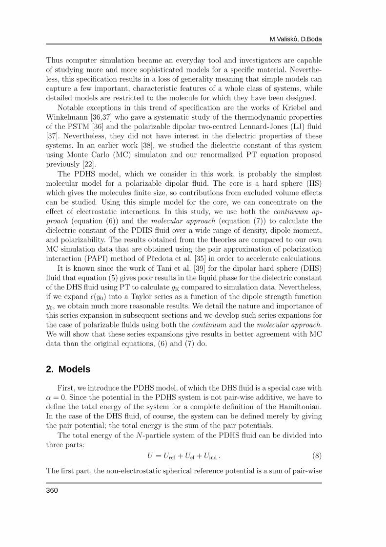
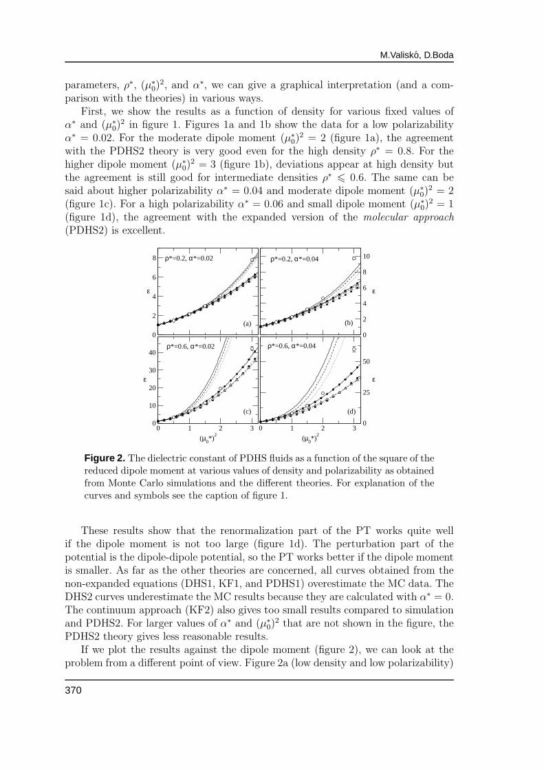
Figure 2. The dielectric constant of PDHS fluids as a function of the square of thereduced dipole moment at various values of density and polarizability as obtainedfrom Monte Carlo simulations and the different theories. For explanation of thecurves and symbols see the caption of figure 1.

These results show that the renormalization part of the PT works quite wellif the dipole moment is not too large (figure 1d). The perturbation part of thepotential is the dipole-dipole potential, so the PT works better if the dipole momentis smaller. As far as the other theories are concerned, all curves obtained from thenon-expanded equations (DHS1, KF1, and PDHS1) overestimate the MC data. TheDHS2 curves underestimate the MC results because they are calculated with α∗ = 0.The continuum approach (KF2) also gives too small results compared to simulationand PDHS2. For larger values of α∗ and (µ∗

0)2 that are not shown in the figure, the

PDHS2 theory gives less reasonable results.If we plot the results against the dipole moment (figure 2), we can look at the

problem from a different point of view. Figure 2a (low density and low polarizability)

370


shows that the theories using series expansion (DHS2, KF2, and PDHS2) fail at highdipole moments, while the equations that do not use series expansion (DHS1, KF1,and PDHS1) seem to work better. From this we might draw the probably wrongconclusion that the PDHS1 theory works better for low density than the PDHS2theory. It is more probable that at high dipole moments (near (µ∗

0)2 = 3) the whole

PT approach fails. Indeed, if we increase the polarizability to α∗ = 0.04 (figure 2b),even the PDHS1 theory underestimates the MC data. Nevertheless, at this lowdensity (ρ∗ 6 0.2), the values of the dielectric constant are quite small, and there isno big difference between the continuum and the molecular approach.

1.5

1.6

1.7

ε

2

2.25

2.5

2.75

3

ε

6

8

10

ε

10

15

20

ε

0 0.02 0.04 0.06α∗

9

12

15

ε

0 0.02 0.04 0.06α∗

20

30

40

ε

(b) ρ*=0.4, (µ0*)

2=0.5

(c) ρ*=0.6, (µ0*)

2=1 (d) ρ*=0.8, (µ

0*)

2=1

(a) ρ*=0.2, (µ0*)

2=0.5

(e) ρ*=0.4, (µ0*)

2=2 (f) ρ*=0.6, (µ

0*)

2=2

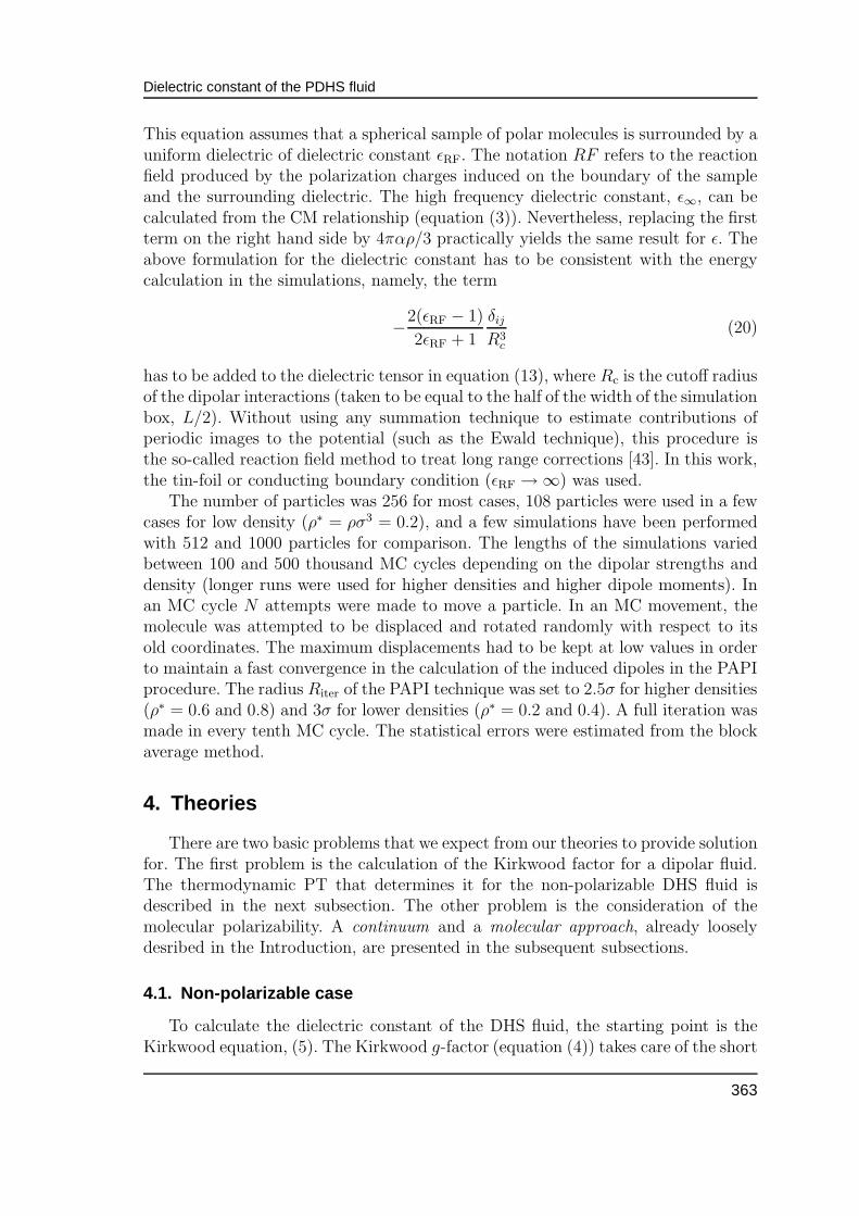
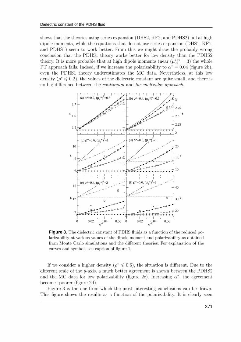
Figure 3. The dielectric constant of PDHS fluids as a function of the reduced po-larizability at various values of the dipole moment and polarizability as obtainedfrom Monte Carlo simulations and the different theories. For explanation of thecurves and symbols see caption of figure 1.

If we consider a higher density (ρ∗ 6 0.6), the situation is different. Due to thedifferent scale of the y-axis, a much better agreement is shown between the PDHS2and the MC data for low polarizability (figure 2c). Increasing α∗, the agreementbecomes poorer (figure 2d).

Figure 3 is the one from which the most interesting conclusions can be drawn.This figure shows the results as a function of the polarizability. It is clearly seen

371

M.Valisko, D.Boda

that the DHS1 and DHS2 theories fail to account for the increase in the dielectricconstant due to the increase of the polarizability of the molecules. At α∗ = 0, thethree theories become equivalent.

Figures 3a and 3b shows results for a very small dipole moment ((µ∗0)

2 = 0.5).Surprisingly, especially for the low density case (ρ∗ 6 0.2), the continuum approach(KF2) gives better results than the molecular approach (PDHS2). The question ari-ses whether it is a coincidence or it has a theoretical basis. We argue that the latteris the case. Since the density and the dipolar strength are low, the dielectric con-stant has small values: the molecules are weakly polar. In this regime, it would notbe surprising if the continuum approach gave reasonable results. However, since thePDHS2 approach uses a renormalization procedure, it is possible that it overesti-mates the effective dipole moment which results in an overestimation of the dielectricconstant. Increasing the density, the molecular approach becomes better (figure 3b).

If we increase the dipole moment to the higher, but still low, value of (µ∗0)

2 = 1,we can see that PDHS2 theory is superior over the others even for high densities(figures 3c–d). Figures 3c–d show that the theories that do not use series expansion(DHS1, PDHS1, and KF1) overestimate the relative permittivity even if α∗ = 0.They describe the α∗-dependence of the dielectric constant similarly as their seriesexpanded counterparts. Increasing the dipole moment even further ((µ∗

0)2 = 2), the

failure of the DHS1, PDHS1,and KF1 theories becomes more apparent as seen infigures 3e–f. At this higher dipole moment, the PDHS2 theory becomes less accurateas the polarizability and the density is increased.

From the figures and the data of table 1 it can be concluded that the dielectricconstant is very sensitive to the polarizability. Both simulations and theory predictthat ε is about 2-3 times larger for α∗ = 0.06 than for the non-polarizable fluid. Thisis a property of the model as was pointed out by other authors before. An insightinto this behaviour can be gained by examining the contributions of the permanentdipoles, the induced dipoles, and the cross term between them to the mean squarepolarization (〈m2

0〉, 〈m2ind〉, and 2〈m0mind〉) as functions of α∗ (see table 1). The

increase of 〈m20〉 with α∗ is moderate, the increase of 〈m2

ind〉 is steep but the absolutevalue remains small. On the contrary, the cross term increases steeply with α, and itseems to bear the main responsibility for the strong α-dependence of the dielectric

Table 2. Monte Carlo results at various N and Riter for the point ρ∗ = 0.8,(µ∗

0)2 = 2, and α∗ = 0.06.

N Riter/σ 〈m20〉 2〈m0mind〉〈m2

ind〉〈m2〉 ε (µ∗0)

2

256 2.00 15.1068 9.6544 1.55872 26.31.2 89.94.0 3.114256 2.50 13.9755 8.9336 1.44558 24.31.0 83.33.2 3.117256 3.00 12.7161 8.1239 1.31463 22.11.1 76.03.6 3.119256 3.42 15.2681 9.7853 1.58585 26.61.4 90.94.8 3.120512 2.50 14.0379 9.0251 1.46582 24.51.4 83.94.6 3.1191000 2.50 14.7461 9.5340 1.55972 25.81.1 88.33.6 3.121

372


constant. This behaviour implies a very strong correlation between the permanentand induced dipoles. For real matters, the α-dependence seems not to be so strongas was found for this model. Moreover, in most cases, α is not a scalar, but a tensor,the effect of which we intend to study in future works.

Table 2 shows the data of an analysis on the dependence of the dielectric prop-erties on the system size and the parameter Riter. We have chosen a PDHS point forthis purpose with a relatively large dipole moment and polarizability at the highestreduced density. The results obtained for the various values of N and Riter fluctuatewithin an error bar that roughly corresponds to that obtained from the block averagemethod. This implies that the N - and Riter-dependence of the dielectric constant isnot too strong at this state point.

0 10 20 30 40 50N

STEP/10000

60

80

100

120

140

ε

N=1000, Riter

=2.5σN=512, R

iter=2.5σ

N=256, Riter

=3.42σN=256, R

iter=3.0σ

N=256, Riter

=2.5σN=256, R

iter=2.0σ

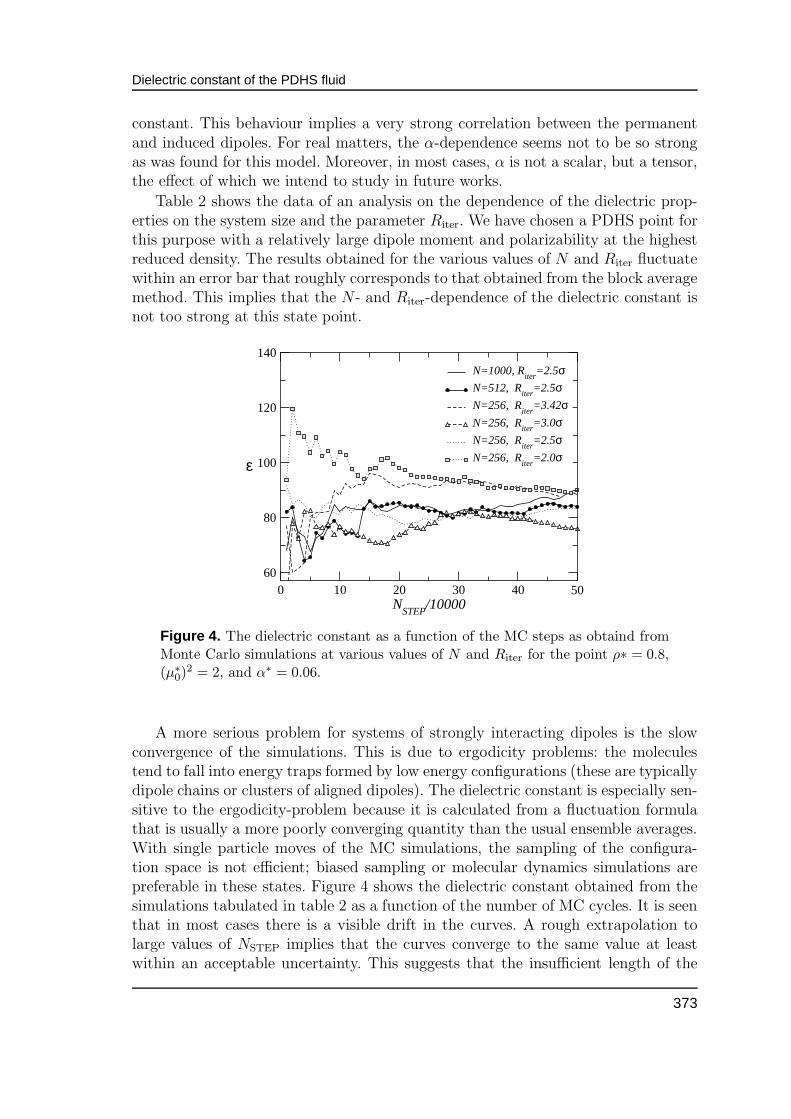
Figure 4. The dielectric constant as a function of the MC steps as obtaind fromMonte Carlo simulations at various values of N and Riter for the point ρ∗ = 0.8,(µ∗

0)2 = 2, and α∗ = 0.06.

A more serious problem for systems of strongly interacting dipoles is the slowconvergence of the simulations. This is due to ergodicity problems: the moleculestend to fall into energy traps formed by low energy configurations (these are typicallydipole chains or clusters of aligned dipoles). The dielectric constant is especially sen-sitive to the ergodicity-problem because it is calculated from a fluctuation formulathat is usually a more poorly converging quantity than the usual ensemble averages.With single particle moves of the MC simulations, the sampling of the configura-tion space is not efficient; biased sampling or molecular dynamics simulations arepreferable in these states. Figure 4 shows the dielectric constant obtained from thesimulations tabulated in table 2 as a function of the number of MC cycles. It is seenthat in most cases there is a visible drift in the curves. A rough extrapolation tolarge values of NSTEP implies that the curves converge to the same value at leastwithin an acceptable uncertainty. This suggests that the insufficient length of the

373

M.Valisko, D.Boda

simulations (arising from nonergodicity) is more crucial in these simulations thanthe value of N or Riter.

Apart from considering tensorial polarizability, another interesting continuationof this study is to calculate the dielectric constant of mixtures of polar molecules.This issue was considered in our earlier paper [60], where we extended our continuumapproach to mixtures and showed that it correctly reproduces the mole fractiondependence of the relative permittivity as obtained from experiments [62]. With areasonable equation for the ε(x) function, we can determine the composition of polarmixtures from simple dielectric measurements.

References

1. Kirkwood J.G., J. Chem. Phys., 1939, 7, 911.2. Onsager L., J. Am. Chem. Soc., 1936, 58, 1486.3. Debye P. Polar molecules. New York, The Chemical Catalouge Company, Dover, 1929.4. Frohlich H. Theory of Dielectrics. 2nd edition, Calderon Press, 1958.5. Wertheim M.S., Molec. Phys., 1973, 25, 211; 1973, 26, 1425; 1977, 33, 95; 1977, 34,

1109; 1978, 36, 1217; 1979, 37, 83.6. Venkatasubramanian V., Gubbins K.E., Gray C.G., Joslin C.G., Molec. Phys., 1984,

52, 1411.7. Joslin C.G., Gray C.G., Gubbins K.E., Molec. Phys., 1985, 54, 1117.8. Gray C.G., Joslin C.G., Venkatasubramanian V., Gubbins K.E., Molec. Phys., 1985,

54, 1129.9. Carnie S.L., Patey G.N., Molec. Phys., 1982, 47, 1129.

10. Caillol J.M., Levesque D., Weis J.J., Kusalik P.G., Patey G.N., Molec. Phys., 1985,55, 65.

11. Zwanzig R.W., J. Chem. Phys., 1954, 22, 1420.12. Pople J.A., Proc. R. Soc. Lond., 1954, A221, 498.13. Barker J.A., Henderson D., J. Chem. Phys., 1967, 47, 2856.14. Barker J.A., Henderson D., J. Chem. Phys., 1967, 47, 4714.15. Barker J.A., Henderson D. – In Proc. of the Fourth Symposium on the Thermodynamic

Properties, edited by Moszynski J.R. 30, ASME, New York, 1968.16. Barker J.A., Henderson D., Smith W.R., Phys. Rev. Lett., 1968, 21, 134.17. Barker J.A., Henderson D., Smith W.R., Molec. Phys., 1969, 17, 579.18. Gubbins K.E, Gray C.G., Molec. Phys., 1972, 23, 187.19. Rushbrooke G.S, Stell G., Høoye J.S., Molec. Phys., 1973, 26, 1199.20. Barker J.A., Henderson D., Rev. Mod. Phys., 1976, 48, 587.21. Gray C.G., Gubbins K.E. Theory of Molecular Fluids. Clarendon Press, Oxford, 1984.22. Valisko M., Boda D., Liszi J., Szalai, I., Molec. Phys., 2002, 100, 3239.23. Vesely F.J., J. Comput. Phys., 1976, 24, 361.24. Vesely F.J., Chem. Phys. Lett., 1976, 56, 390.25. Patey G.N., Torrie G.M., Valleau J.P., J. Chem. Phys., 1979, 71, 96.26. Pollock E.L., Alder B.J., Patey G.N., Physica A, 1981, 108, 14.27. Mooij G.C.A.M., de Leeuw S.W., Williams C.P., Smit B., Molec. Phys., 1990, 71, 909.28. Jedlovszky P., Palinkas G., Molec. Phys., 1995, 84, 217.29. Kiyohara K., Gubbins K.E., Panagiotopoulos A.Z., J. Chem. Phys., 1997, 106, 3338.

374


30. Medeiros M., Costas M.E., J. Chem. Phys., 1997, 107, 2012.31. Millot C., Soetens J.-C., Martins Costa M.T.C., Molec. Sim., 1997, 18, 367.32. Kiyohara K., Gubbins K.E., Panagiotopoulos A.Z., Molec. Phys., 1998, 94, 803.33. Jedlovszky P., Richardi J., J. Chem. Phys., 1999, 110, 8019.34. Jedlovszky P., Mezei, M., Vallauri R., J. Chem. Phys., 2001, 115, 9883.35. Predota M., Cummings P.T., Chialvo A.A., Molec. Phys., 2001, 99, 349; 2002, Ibid.,

100, 2703.36. Kriebel C., Winkelmann J., Molec. Phys., 1996, 88, 559.37. Kriebel C., Winkelmann J., J. Chem. Phys., 1996, 105, 9316.38. Valisko M., Boda D., Liszi J., Szalai I., Molec. Phys., 2003, 101, 2309.39. Tani A., Henderson D., Barker J.A., Hecht C.E., Molec. Phys., 1983, 48, 863.40. Allen M.P., Tildesley D.J. Computer Simulation of Liquids. Oxford, New York, 1987.41. Frenkel D., Smit B. Understanding Molecular Simulations. Academic Press, San Diego,

1996.42. Sadus R.J. Molecular Simulation of Fluids: Theory, Algorithms, and Object-

orientation. Elsevier, Amsterdam, 1999.43. Barker J.A., Watts R.O., Chem. Phys. Lett., 1973, 26, 789.44. Gray C.G., Gubbins K.E., Mol. Phys., 1975, 30, 1481.45. Rushbrooke G.S., Mol. Phys., 1979, 37, 761.46. Murad S., Gubbins K.E., Gray C.G., Chem. Phys., 1983, 81, 87.47. Goldman S., Mol. Phys., 1990, 71, 491.48. Jepsen D.W., J. Chem. Phys., 1966, 44, 774.49. Jepsen D.W., J. Chem. Phys., 1966, 45, 709.50. Rushbrooke G.S., Mol. Phys., 1981, 43, 975.51. Van Vleck J.H., J. Chem. Phys., 1937, 5, 556.52. Wertheim M.S., J. Chem. Phys., 1971, 55, 4291.53. Szalai I., Chan K.Y., Henderson D., Phys. Rev. E, 2000, 62, 8846.54. Kronome G., Szalai I., Liszi J., J. Chem. Phys., 2002, 116, 2067.55. Szalai I., Chan K.Y., Tang Y.W., Mol. Phys., 2003, 101, 1819.56. Steven M.J., Grest G.S., Phys. Rev. Lett., 1994, 72, 3686.57. Boda D., Winkelmann J., Liszi J., Szalai I., Mol. Phys., 2003, 101, 1819.58. Kristof T., Szalai I., Phys. Rev. E, 2003, 68, art.no. 041109.59. Kristof T., Liszi J., Szalai I., Phys. Rev. E, 2004, 69, art. no. 062106.60. Valisko M., Boda D., Liszi J., Szalai I., Phys. Chem. Chem. Phys., 2001, 3, 2995.61. Valisko M., Boda D., J. Phys. Chem. B, 2005, 109, 6355.62. Szalai I., Laszlo-Paragi M., Ratkovics, F., Monats. Chem., 1989, 120, 413.

375

M.Valisko, D.Boda

Монте Карло та теоретичне вивчення діелектричної

сталої рідини поляризаційних дипольних твердих

сфер

М.Валізко, Д.Бода

Університет Вешпрем, Угорщина

Отримано 29 жовтня 2004 р.

Приведено результати систематичного вивчення методом Монте

Карло (МК) та теорії збурень (ТЗ) діелектричної сталої рідини пол-яризаційних дипольних твердих сфер. Поляризація молекул врахов-ується двома способами. У підході неперервного середовища пост-ійний диполь молекули поміщається у сферу з діелектричною

сталою ε∞, так як це робиться Онзагером. Високочастотна діелек-трична стала ε∞ рахується зі співвідношення Клаузіса-Мозотті,тоді як діелектрична стала поляризаційної рідини отримується з

рівняння Кірквуда-Фройліха. У молекулярному підході поляризац-ія враховується на молекулярному рівні, внаслідок чого взаємодії

не є парно адитивними. Для розрахунку індикованого дипол-ьного моменту використовується ренормалізаційний метод ТЗ Вер-тхайма, а для діелектричної сталої використовується оригінальна

формула [22]. Ми також застосовуємо групові розклади для діелек-тричної сталої в обох підходах. Групові розклади забезпечують

кращу узгодженість з комп’ютерними результатами. Узгодженість

між МК даними і результатами ТЗ є дуже доброю у діапазоні

низьких та середніх дипольних моментів та поляризації. Для сил-ьних дипольних взаємодій проявляються проблеми ергодичності

та анізотропної поведінки і комп’ютерні дані стають сумнівними, а

теоретичні результати – необгрунтованими.

Ключові слова: діелектрична константа, Монте Карло,полімеризований флюїд

PACS: 61.20.Gy, 61.20.Ja, 61.20.Ne

376

dielectric constant of the polarizable dipolar hard sphere

Documents