Did Quantitative Easing only inflate stock prices? Macroeconomic

evidence from the US and UK∗

Mirco Balatti†, Chris Brooks‡, Michael P. Clements§ and Konstantina Kappou¶

This version: January 2017

ABSTRACT

This paper considers the impact of US and UK Quantitative Easing (QE) on their respective

economies with a particular focus on the stock market, production and price levels. We conduct an

empirical quantitative exercise based on a novel six-variable VAR model, which combines macroeco-

nomic and forward-looking financial variables and uses a ‘pure’ measure of QE. The results suggest

a positive response of equity prices and bid-ask spreads and an inverted ‘V’ shaped reaction of

volatility to the monetary stimulus. Output and inflation, in contrast with some previous studies,

show an insignificant impact providing evidence of the limitations of the central bank’s programmes.

We attribute the variation to this difference in our modelling approach, which includes stock market

variables, and we conclude that its presence is of critical importance in the assessment of unconven-

tional monetary policy. Economically, we argue that the reason for the negligible economic stimulus

of QE is that the money injected funded financial asset price growth more than consumption and

investments.

JEL classification: C32, C54, E51, E58, G1.

Keywords: Quantitative Easing, Monetary Policy, Stock Market, Vector Autoregression.

∗First version: September 2016. Mirco Balatti, Chris Brooks, Michael P. Clements and Konstantina Kappou areat the ICMA Centre, Henley Business School. Address: ICMA Centre, Henley Business School, Whiteknights Park,P.O. Box 242, Reading RG6 6BA, United Kingdom.Acknowledgements: We thank Torben Andersen, Lawrence Christiano, Giorgio Primiceri, Matt Roberts-Sklar andViktor Todorov as well as Quantitative Finance seminar participants at Kellogg School of Management, NorthwesternUniversity for helpful comments and suggestions. The first author acknowledges financial support from the Economicand Social Research Council [grant number ES/J500148/1]†Email: mirco.balatti@pgr.icmacentre.ac.uk.‡Email: c.brooks@icmacentre.ac.uk.§Email: m.p.clements@icmacentre.ac.uk. Michael P. Clements is also at the Institute for New Economic Thinking,

Oxford Martin School, University of Oxford.¶Email: k.kappou@icmacentre.ac.uk.

“Some of the optimism in the financial markets, [...] may not be consistent with the speed at

which the underlying data are likely to change” - Lord King, Former BoE Governor (February 2013)

I. Introduction

In the aftermath of the 2008 financial crisis, central banks around the world adopted both

conventional and non-conventional measures in the hope of alleviating the deepest recession since

1929 and taking the economy back to pre-crisis levels. Initially, central banks acted as lenders of

last resort, providing liquidity, accepting more risky and less liquid collateral, thereby effectively

implementing a Qualitative Easing (not to be confused with Quantitative Easing) and cutting

short term nominal interest rates (Lenza, Pill, and Reichlin, 2010; Gagnon et al., 2010). The zero

lower bound (ZLB)1 was rapidly reached, yet the economic outlook still worsened and issues in the

financial sector (e.g. credit (un)availability) persisted. The lending market was still frozen, the

unemployment level too high, GDP growth and inflation too low (Dudley, 2010). After the collapse

of Lehman Brothers, major central banks therefore decided to embark on additional unconventional

monetary policy, in order to revitalize the real economy. The actions taken after September 2008

included both changes to the central bank balance sheet composition (Qualitative Easing) and size

(Quantitative Easing). Lenza, Pill, and Reichlin (2010) argue that there are similarities in the

evolution of the balance sheets of the Federal Reserve Bank (FED), the Bank of England (BoE)

and the European Central Bank (ECB), namely an expansion in the proportion of unconventional

to conventional assets and the nature of liabilities. The Federal Open Market Committee (FOMC),

an organ of the US central bank, pioneered large scale direct market interventions by buying

mortgage backed securities (MBS), agency debt and treasury debt to the value of hundreds of

billions of US dollars.2 Other central banks such as the BoE, the ECB, the Bank of Japan, the

Swiss National Bank and the Swedish National Bank also undertook open market operations,

thereby vastly enlarging their balance sheets.

By early 2015, the equity market indices of major economies such as the S&P 500, the FTSE

100 and the DAX 30 not only regained their crisis losses, but also touched new historical nominal

highs.3 On the other hand, however, macroeconomic fundamentals, and inflation in particular, were

still sluggish at the end of 2015.4 In fact, base interest rates around the world are still found at the

ZLB (or even lower), although some people express concerns of economic overheating,5 whilst the

ECB is still implementing its QE policy and the BoE has initiated a third QE round, after having

1. By ZLB we refer to that condition where a central bank intends to stimulate the economy by lowering short-terminterest rates but faces a constraint when nominal rates reach zero. See, for example, McCallum (2000).

2. The Bank of Japan had implemented alternative monetary measures like QE to address domestic deflation inthe late 1990s. Yet, the Japanese QE unlike the US, UK and Eurozone QEs, entailed an expansion of the liabilityside of the central bank balance sheet rather than the asset side Bernanke (2009).

3. The S&P 500 also touched new levels in real (inflation-adjusted) terms.4. September 2015 inflation figures: US 0.00%; UK -0.10%; Germany 0.00%. (Source: US Bureau of Labor

Statistics, Office for National Statistics, Federal Statistics Office)5. See, for instance, Yellen (2015) speech and ‘Goldman warns of risk of US economic overheating’ Financial Times

(2015, November 9).

2

cut the base rate again in August 2016 to 0.25%.

There is widespread interest in Quantitative Easing in the media. Whilst some articles refrain

from speculating over its effectiveness since “it is hard to separate the effects of QE from other

factors”,6 others take a stand against QE implementation and warn that “stock market bubbles of

historic proportions are developing in the US and UK markets”.7 Even Mervyn King, former Bank

of England Governor, said that he was “concerned that some of the optimism of financial markets,

[...] may not be consistent with the speed at which the underlying data are likely to change”.

In the academic world, the hypothesized effects of such a novel monetary policy began to be

studied before the US QE took place and divide economists into three factions. One strand follows

new Keynesian models and is sceptical about the macroeconomic effects of Quantitative Easing.

Such is true of Eggertsson and Woodford (2003), who put forward an ‘irrelevance proposition’ of

open market operations. They argue that at the ZLB, non-interest-bearing money is a perfect sub-

stitute for interest-bearing assets (e.g. ‘bullet’ bonds). The second strand allows for market frictions

and claims that QE can indeed have economic implications (e.g. Mankiw and Reis, 2002). Finally, a

third perspective emphasises the ineffectiveness of the unconventional monetary policy employed in

Japan, by introducing credit in standard macroeconomic models. Indeed, Werner (2012) proposes a

‘Quantity Theory of Credit’ empirically supported by Lyonnet and Werner (2012). Krishnamurthy

and Vissing-Jorgensen (2011) conduct a detailed empirical analysis of the means through which US

QE1 and QE2 have worked, namely: signalling, safety, inflation, duration, liquidity, prepayment

and default. They conclude that different channels are altered by non-conventional monetary policy

and assets are affected heterogeneously. More recently, Williams (2016), the president of the San

Francisco Fed, has called for a critical reassessment of the effectiveness of central banks’ monetary

policy. The issue of the efficacy of unconventional monetary policy is clearly of much interest among

the general public, practitioners, policy makers and academics.

Scholarly papers have tried to evaluate empirically the impact and effectiveness of QE policies on

interest rates such as bond yields and mortgage rates, mainly in the US – QE1 and QE2 – (D’Amico

and King, 2013; Hamilton and Wu, 2012; Gagnon et al., 2010; Hancock and Passmore, 2011) and the

UK (Breedon, Chadha, and Waters, 2012; Bridges and Thomas, 2012; Joyce et al., 2011). Following

Voutsinas and Werner (2010), the above literature can be grouped under the umbrella term ‘input

performance’, i.e. the central bank policy impact on interest rates. Though informative and useful,

this strand of literature has shifted the definition of monetary policy effectiveness from the final

target, the macroeconomic impact, to an intermediate target, yields. The ‘output performance’

literature, instead, looks at the ultimate goal of the policy such as price stability and/or output

growth. By contrast, only a few studies have been devoted to the analysis of the output and

price levels effects.8 Lastly, other researchers (Neely, 2010; Fratzscher, Lo Duca, and Straub, 2013;

Bhattarai, Chatterjee, and Park, 2015) have also looked at spillover effects from the US to other

6. Claire, Jones. (2013, October 18). Did QE only boost the price of Warhols? Financial Times.7. Chang, Ha-Joon. (2014, February 24). This is no recovery, this is a bubble - and it will burst. The Guardian.8. Examples of this second strand of literature include Kapetanios et al. (2012), Bridges and Thomas (2012), and

Gambacorta, Hofmann, and Peersman (2014).

3

countries.

A number of methodological approaches, such as event study analysis and time series regressions,

have been applied to disentangle the effects of QE from other exogenous innovations. The isolation

of the policy repercussion in event studies is achieved in a temporal manner. By employing high

frequency data, spikes in trading volumes or returns are detected and attributed to QE events, and

the causal effect of the monetary policy is assumed. The computed price/yield changes around

the announcement day or time are summed and the cumulative differences are taken to represent

the influence of the policy. This approach is used in studies such as D’Amico and King (2013)

and Fratzscher, Lo Duca, and Straub (2013), who have also shown that both the announcement

and the implementation of QE can alter prices and yields. Rogers, Scotti, and Wright (2014) also

found evidence of asymmetries in the effects of expansionary and contractionary unconvnetional

monetary policy. Event study analysis around announcement dates is perhaps the most popular in

this strand of literature (Gagnon et al., 2010; Krishnamurthy and Vissing-Jorgensen, 2011; Joyce

et al., 2011; Rogers, Scotti, and Wright, 2014) given its simplicity. Yet, it suffers from a number

of drawbacks. First, the arbitrary length of the event window might be too small to capture all

the impact of the announcement or too long and include other news. There might also be news

on the same day as the QE that affects prices, which can lead to under- or over-estimation of the

effect of the monetary policy. Second, event study analysis is based on the strong assumption that

markets efficiently and rapidly adjust to the news. This may not be the case in a tumultuous

environment as in the wake of the 2008 financial crisis, where the market was suffering from a

lack of liquidity. Thirdly, price/yield changes around QE news would only capture the difference

between the average market expectation and the actual update. If, as was the case for the latest

US QE announcements, the market estimates already priced in were close to the actual news, an

event study approach would wrongly reveal little, if any, impact. Lastly, the application of event

study analysis may be valid on daily (or intra-day) time series, such as financial data, but may be

more problematic with monthly or quarterly macroeconomic statistics.

Another technique to disentangle those price innovations caused by the monetary policy from

those due to other factors (e.g. changes in the macroeconomic fundamentals and market envi-

ronment) involves estimating vector autoregression (VAR) models to capture complex economic

dynamics, and includes the analysis of counterfactual scenarios to estimate the influence. This is

the approach used for instance in Lenza, Pill, and Reichlin (2010), Kapetanios et al. (2012), and

Gambacorta, Hofmann, and Peersman (2014), and is also our methodology. In general, time series

approaches may alleviate concerns about the window length to be employed in an event study,

and they may also counter the scepticism regarding the time it takes distressed markets to ‘digest’

policy news. Lastly, low frequency (e.g. monthly and quarterly) macroeconomic time series can be

included in the analysis.

Overall, notwithstanding the variety of methodologies employed, there is a general agreement

that QE measures in the US and UK have had a positive impact on their respective economies,

although the magnitudes of the effects vary across the literature. Lyonnet and Werner (2012),

4

Werner (2012), and Engen, Laubach, and Reifschneider (2015) are perhaps the discordant voices

since they argue that the BoE and FED QEs had limited effect on the British and US economies,

respectively.

Thus, so far, scholarly papers have focused on assessing empirically whether Quantitative Easing

has been a successful policy instrument in lowering Treasury, agency and corporate bond and MBS

yields and to a lesser extent in promoting GDP growth, employment and inflation. To the best of

our knowledge, very few papers (Joyce et al., 2011; Fratzscher, Lo Duca, and Straub, 2013; Bridges

and Thomas, 2012), have touched upon the effects of QE on equity markets. Their estimates are,

de facto, not the core results of the respective analyses and their samples do not include all rounds

of QE.

The main contributions of this paper lay in the fact that we combine an ‘input’ and ‘output’

performance analysis by including (lower frequency, monthly) macroeconomic variables with (higher

frequency, daily) financial ones in a single VAR framework. Regarding the latter, this allows us to

study the impact of QE on the stock market in a holistic and multi-faceted fashion as we study

prices, volatility and liquidity. With respect to the former, we find that the inclusion of financial

variables, which could be regarded as a channel of transmission of the policy, to be of key importance

for monetary policy assessment and suggesting that the models estimated in previous studies may

have suffered from omitted variable bias and would therefore have been mis-specified. Our findings

also show that this is the driver of the difference in results with some of the previous literature.

Further, unlike previous studies on unconventional monetary policy evaluation, we employ a

‘pure’ and direct measure of QE, namely the amount of securities held outright by the FED and

BoE, in a model that encompasses stock market metrics as well as macroeconomic variables. When

producing impulse responses, this allows a direct modelling of the unconventional monetary policy

shock rather than indirectly through a ‘channel’ variable, like the 100bp reduction in government

bonds used in Kapetanios et al. (2012), which relies on the Joyce et al. (2011) estimates.

We also fill a gap in the literature by assessing the impact of QE on a range of macroeconomic

and financial variables using a time series approach that covers all rounds of QE implemented in

the UK and US until 2015. The inclusion in our study of the UK in addition to the US allows a

comparison between two countries of very different size and weight in the world economy and the

different timing in the respective policy implementation.

Our assessment is carried out by vector autoregressive modelling to capture the linkages among

macroeconomic variables – production and inflation – and financial market variables – the stock

market level, volatility and liquidity. We argue that such a VAR enables a well-rounded assessment

of Quantitative Easing as implemented in the US and UK, from the equity market repercussions

to the ultimate targets of the policies, i.e. output and inflation. In a nutshell, we find that on the

one hand QE boosted equity prices significantly and reduced its volatility in the medium term (4-5

months). On the other hand, the unconventional stimulus struggled to propel the macroeconomy.

Interestingly, we also note that the US QE appears to have been more effective than its UK

counterpart.

5

The analysis conducted and our results are of the utmost importance for policy makers around

the world and in particular for the Bank of England given their stated intention to undertake

further rounds of monetary stimulus following the outcome of the ‘Brexit’ referendum.9

The rest of the paper is organised as follows. Section 2 describes the dataset used in the

analysis and the chosen QE variable. Section 3 outlines the econometric framework employed for

the estimation of the VAR models and the impulse response analysis. In Section 4, we present

the main findings on QE impact estimates. Section 5 explains the empirical results by analysis a

channel of transmission and provides a comparison with the previous literature. Section 6 contains

some robustness tests and Section 7 concludes.

II. Data

The dataset we employ in the exercise includes six variables with monthly observations for each

of the two countries. It comprises macroeconomic variables, namely the index of real industrial

production and inflation, stock market variables such as equity prices, market volatility and liquidity

and the Quantitative Easing variable. Such a dataset allows us to analyse the financial and economic

impacts, thereby also capturing any linkages between the two. The data sources are Datastream

and FRED. The time span of the dataset covers the period from June 1982 to November 2014 for

the UK and from January 1971 to November 2015 for the US. All variables are in log-levels except

volatility and liquidity, which we divide by 100.10

We follow Bernanke, Boivin, and Eliasz (2005), in using industrial production and the consumer

price index (CPI) to proxy for output and inflation respectively.11 In the spirit of Bhattarai,

Chatterjee, and Park (2015), we use the amount of securities held outright by the central banks.

Using the quantity of assets bought by the BoE and the FED allows us to capture QE directly,

rather than using other variables that were affected by the policy such as interest rates. This leads

us to extend the Quantitative Easing time series, in the first part of the sample where no data on

securities held is available, with M0, since it is a narrow money metric.12 For the stock market,

the FTSE All-Share and the S&P 500 represent the UK and the US respectively. Market volatility

is computed as a 30-day rolling standard deviation of log daily returns. Lastly, in the spirit of

Goyenko, Holden, and Trzcinka (2009), we calculate stock market liquidity using Roll (1984), again

from daily equity market data.13 Roll (1984) provides a bid-ask spread estimate, thus the higher

our measure the lower the market liquidity.

The ordering of the variables for identifying ‘structural’ shocks in the VAR analysis via a

Cholesky decomposition, is largely in line with the literature (see for example, Kapetanios et

9. See, for example, Andy, Bruce. (2016, July 13). Bank of England readies new blast of QE for post-BrexitBritain. Reuters.

10. Where possible, we use seasonally adjusted variables.11. We use UK RPI rather than CPI as the inflation proxy, because of data availability constraints.12. We show in Section VI and Appendix D that our results are not driven by our choice of augmenting the QE

time series with M0. Indeed, re-estimating the model over the period where there is data availability on QE amountsleads to similar conclusions.

13. As is customary in the literature, we substitute the Roll measure with zero when the autocovariance is positive.

6

al., 2012; Banbura, Giannone, and Reichlin, 2010; Lenza, Pill, and Reichlin, 2010), with slow

macroeconomic variables followed by the monetary policy instrument and fast financial variables

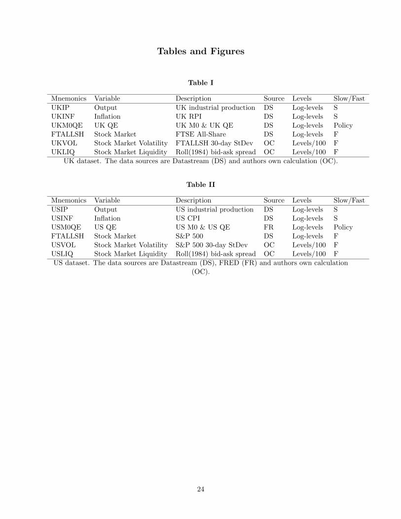
at the bottom. Tables I and II provide a detailed description of the datasets.

[Place Table I about here]

[Place Table II about here]

III. Methodology

Determining the impact of Quantitative Easing is a challenging task as it requires isolating

the effect of the monetary policy from the influence of other variables. Vector autoregressive

frameworks have been used widely by researchers to assess the effects of conventional monetary

policy (Christiano, Eichenbaum, and Evans, 1999) in the US as well as unconventional monetary

policy in the Euro area (Lenza, Pill, and Reichlin, 2010). In this paper, we adopt a VAR approach

to examine the repercussions of Quantitative Easing in the UK and the US on macroeconomic and

stock market variables. This allows us to exploit the time series dimension of our dataset of more

than 30 years of historical monthly data, thereby reducing model uncertainty. We conduct the

overall approach of this investigation in three steps:

1. Construct and estimate a VAR model with the aforementioned variables, in order to capture

the dynamics of the UK and US economies.

2. Identify Quantitative Easing shocks as exogenous orthogonal innovations of the QE variables.

3. Apply shocks to the QE variables and compute the impulse response functions (IRF) of the

variables in the model.

A. Vector autoregressive model

The reduced form VAR model we adopt is of the type:

Yt = C + β0t+ β1Yt−1 + β2Yt−2 + ...+ βpYt−p + εt

εt ∼ N(0,Σ)(1)

where Yt is an n× 1 vector of endogenous variables, C is an n× 1 vector of unknown constants, β0

is an n × 1 vector of time-trend parameters, β1, ..., βp are n × n matrices of unknown parameters,

and εt is an n × 1 vector of disturbances. εt is assumed to be uncorrelated over time, but Σ is

expected to be non-diagonal.14

14. We expect the variance-covariance matrix of the vector of disturbances in the standard VAR to be non-diagonalas our VAR is a reduced form and does not condition on contemporaneous information. Equally, the cross-correlationscannot be exploited in estimation to generate better estimates. Indeed, the OLS estimation equation by equationof the VAR is optimal. Thus, since reduced form VAR disturbances are a combination of structural shocks, thenon-diagonal elements of the variance-covariance matrix can take non-zero values.

7

As we focus on the domestic impact of Quantitative Easing, we estimate the model individually

for the two economies. Furthermore, the variables are entered in log-levels since they might be

characterised by unit roots; this approach implicitly admits possible cointegrated relationships

among the variables (Sims, Stock, and Watson, 1990).

Our rather long sample period allows a variable-rich specification, which enables us to better

capture the QE period dynamics. The aim is to model the macroeconomic features (industrial pro-

duction and inflation) jointly with the stock market variables (equity prices, liquidity and volatility).

The inclusion of stock market volatility serves a dual purpose. Not only can it offer further in-

sight into the capital market consequences of the unconventional monetary policy, but it is also

relevant in identifying the exogenous and autonomous innovations of the amount of securities held

by the central banks from the endogenous and automatic responses of central bank balance sheets

to market uncertainty and risk peaks as Gambacorta, Hofmann, and Peersman (2014) suggest.

B. Identification

Quantitative Easing shocks are identified as exogenous orthogonal innovations of the QE vari-

ables. For this purpose, we order the variables as in Tables I and II and distinguish between slow (S)

and fast (F) moving variables following (Christiano, Eichenbaum, and Evans, 1999). The former

group includes macro variables, whereas the latter comprises financial variables. We assume that

fast moving variables respond contemporaneously to monetary policy shocks, whilst slow moving

ones only respond with a one period lag. As suggested by Bjørnland and Leitemo (2009), it is im-

portant to jointly consider monetary policy and financial variables when analysing monetary policy

transmissions. A Cholesky ordering that puts financial variables before the monetary instruments,

thereby restricting the influence of a policy to lagged response, would be inadequate and could

potentially bias results.

Formally, we compute the lower triangular Cholesky decomposition of the variance-covariance

matrix of the VAR residuals. The identification strategy implies that each variable responds contem-

poraneously to the orthogonalized shock to variables ordered above it. Hence placing QE between

the slow macro and fast financial variables implies that the financial variables respond contempo-

raneously to a QE shock, whereas the macrovariables only respond the following period. Such an

identification scheme has been extensively used in the literature on conventional and unconventional

monetary policy. Examples include Christiano, Eichenbaum, and Evans (1999), Bernanke, Boivin,

and Eliasz (2005), and Banbura, Giannone, and Reichlin (2010). In general, a positive disturbance

to the QE variable can be interpreted as a loosening policy.

C. Model estimates and forecasting ability

This empirical exercise allows us to establish a baseline against which the results of different

specifications, proposed below, can be compared. We estimate VAR models in log-levels via OLS

separately for the UK and the US using the number of lags suggested by the Hannan-Quinn

8

information criterion, i.e. two lags for both countries.15

A forecast evaluation procedure is conducted in order to gauge whether the model is able to

produce competitive forecasts. The framework entails producing recursive forecasts for one and

three months (h = 1, 3) ahead and comparing the projections with actual observations. We analyse

the forecasting power out-of-sample. We reduce the dataset by the forecasting horizon, thereby

estimating the VAR model with fewer data points. More specifically, data until 2011 are used

as the initial sample, with an evaluation period of 2011:11-2015:11 (t =2011:11,...,2015:11). At

each step, the model is re-estimated and forecasts for different horizons are produced using data

from 1982:6 until t − h, for the UK, and from 1971:1 to t − h for the US. We also calculate

the forecasting errors for a random walk (RW) model and calculate Theil’s-U statistic between

the VAR framework and the RW. A value below one indicates greater forecasting power from our

model compared to the RW. The random walk is a challenging benchmark as numerous studies have

shown that many financial and some economic variables behave like a random walk. Should the

VAR model outperform the RW, we can conclude that the model is capable of capturing systematic

relationships between the variables and more generally, that these relationships can be exploited

for forecasting and policy analysis.16

Tables III and IV present the out-of-sample root-mean-square percentage errors (RMSPE) of

point forecasts from the UK and US models respectively.17 Starting with the ‘VAR’ column, it

shows the smallest forecast errors for the two macro variables and market liquidity. On the other

hand, stock market levels, volatility and QE amounts, unsurprisingly, produce larger RMSPEs.

This holds true for both countries and across forecasting horizons. RW forecasting errors also

display a similar pattern.

[Place Table III about here]

[Place Table IV about here]

Let us now turn to comparing the two models. The last column of Table III exhibits only

some Theil’s-U statistics below one, suggesting that the RW is marginally better at one-step ahead

prediction. The conclusion is reversed as we extend the forecasting horizon to three months.

Indeed, the VAR model produces RMSPEs smaller than the benchmark model in the vast majority

of instances. Unreported results at the 6- and 12-month horizons provide further evidence on the

ability of the VAR to produce better forecasts at longer horizons.

Overall, our VARs predict quite well, suggesting that we have constructed plausible models capa-

ble of extrapolating valuable information from the dataset used. More specifically, they outperform

the random walk benchmark on all financial variables (stock market, volatility and liquidity) and

15. Complete estimation results are available upon request.16. Unreported in-sample results show the vast majority of Theil’s-U statistics to be less than unity at 1-, 3-, 6-

and 12-month horizons.

17. RMSPE are calculated as follows. RMSPE =

√∑(yt+h−ft+h

yt+h

)2where ft+h is the expected value of the

variable h steps ahead, forecasted at time t and yt+h is the actual value.

9

most macroeconomic ones (UK output, US inflation and Quantitative Easing for both countries).

In sum, these findings provide support for our modelling choice for both economies.

D. Impulse response analysis

This analysis consists of calculating the impulse responses to a unitary monetary policy shock

in the baseline VAR model for a 24-month horizon. In Figures 1-5 below, we present the 16th

and 84th percentiles of the impulse responses distribution (dotted lines).18 We compute confidence

intervals by 1000 wild bootstrap draws in the spirit of Wu (1986).19

We normalise the size of the shock to match the peak three-fold increase (200%) of the Bank of

England and Federal Reserve balance sheets. Consequently, we give the system a 2-unit disturbance

(equivalent to 200%) in the amount of securities held by the BoE (UKM0QE), which gradually

declines but does not vanish completely over the 2-year horizon. In the case of the US, we apply

a 0.75 unit shock to the FED securities (USM0QE) which rises to a peak equivalent to the 200%

increase after about five months and progressively fades out in just less than two years.20 The results

of this procedure can be considered as an upper bound on the impact of Quantitative Easing since

we assume that the entire QE amount was exogenous, whereas in reality only a fraction of it might

have been unexpected.

A unit increase (decrease) in the response of a log-level variable can be interpreted as a 100%

rise (fall) in the levels. An increase (decrease) of one unit in the response of a variable expressed

as a growth rate should be interpreted in absolute terms (for example, a response of +0.01 in

unemployment is a 1% increase, say from 4% to 5%). The analysis of the magnitude allows us to

perform a cross-country comparison of the sizes of the responses.

IV. Findings

A. The financial market impact

The three plots in the bottom rows of Figures 1 and 2 suggest that Quantitative Easing had

a substantial impact on the domestic capital markets. Starting from the stock market level, both

UK and US equities fell contemporaneously with the QE shock but rose immediately afterwards,

suggesting a strong and significant impact of the monetary policy on stock prices.The immediate

negative response of equities is illustrated by the event study analysis of Joyce et al. (2011). On the

one hand, the signalling message of policy makers who decide to implement such an unconventional

measure might cause investors to revise their future macroeconomic forecasts downwards, thereby

18. The 16% and 84% quantiles are common in macroeconomic VAR models. See, for example, Giannone, Lenza,and Reichlin (2014), Giannone, Lenza, and Primiceri (2015), Gambacorta, Hofmann, and Peersman (2014), andWeale and Wieladek (2016)

19. More recently, the wild bootstrap procedure has been applied, for instance, in Cesa-Bianchi, Thwaites, andVicondoa (2016).

20. Due to the linearity of the model, the size of the shock is irrelevant to the shape and significance of the impulseresponses. Thus, the following analysis is valid and robust to different magnitudes of shocks.

10

decreasing dividend expectations and raising equity risk premia, ultimately causing stock prices

to fall in the short run, immediately after the QE shock. On the other hand, our results on the

positive impact of the monetary policy on the stock market in the longer run match the findings

of Bridges and Thomas (2012), in the UK case and of Fratzscher, Lo Duca, and Straub (2013) for

the US. We argue that the liquidity injected in the markets operated, via lower interest rates as

extensively reported in the literature, through the following mechanisms. First, the present value of

future expected dividends was driven up. Second, firms’ lower borrowing costs translated, ceteris

paribus, into higher profitability and a higher propensity to expand and invest. Third, the low

returns offered in the bond markets resulted in a shifting of investors away from it and towards

the equity market. Overall, the results are consistent with the presence, in the short term, of a

negative signalling channel that causes stock prices to drop and, in the longer run, the prevalence

of positive factors that contribute to higher equity market levels.

Our median estimates indicate a peak impact on equities, at the end of the 24-month horizon,

of around 30% for the FTSE All-Share and around 50% for the S&P 500.21 This implies that the

unconventional policy measures adopted caused increases in equity prices of at least 30%. If the

FTSE was trading at 1000 points, QE boosted it by 300 points over two years. Indeed, the UK and

US stock markets grew by around 44% and 36%, respectively, over the two years following the first

QE annoucement.22 Thus, QE acted on equity markets through time and promoted their growth

on an economically meaningful scale.

Turning to the response of volatility, the shapes of the British and American response functions

are again comparable. The initial impact is significantly positive but turns negative after four to

five months and reaches a peak at seven months in the UK, and at 12 in the US, before returning

to baseline, drawing an inverted ‘V’ shaped response. A quick calculation quantifies the maximum

influence to be between 0.14% and 1.26% in the UK and 0.13% to 2.32% in the US compared to their

respective average volatility levels.23 This result indicates a spike in market turmoil in the shorter

run after a Quantitative Easing shock, perhaps as the markets ‘digest’ the news. The extra volatility

could also simply be due to the higher volumes of trading generated as the excess liquidity finds

its way in the market (Shiller, 1981). In the longer run, instead, the impulse responses indicate a

calmer period (six months to two years), as the injected liquidity seems to settle marginally reducing

equity prices movements. Gambacorta, Hofmann, and Peersman (2014) structural identification

of the impact of QE, implemented by sign restrictions, fails to find the initial increase of market

volatility as the response is bounded to be negative by construction.

Lastly, when we compare the response of market liquidity, a difference between the two economies

21. Note that there were, obviously, other forces acting on equity prices, both positively and negatively, duringthe QE period. The reader should interpret our estimates as an upper bound effect on the growth of stock marketsattributable to the unconventional monetary policy.

22. In January 2009, when the BoE announced the first round of QE the FTSE All-Share was trading at around2150 points and in January 2011, it was trading at 3100 points, which implies an arithmetic growth of around 44%.In November 2008, when the FED announced the first round of QE the S&P 500 was trading at around 880 pointsand in November 2010, it was trading at 1200 points, which implies an arithmetic growth of around 36%.

23. 0.02/14.27 = 0.14% and 0.18/14.27 = 1.26%; 0.02/15.08 = 0.13% and 0.35/15.08 = 2.32%.

11

emerges. We find the UK spread measure to be influenced insignificantly, whilst the US one ap-

pears to increase, reaching a maximum around four months following the shock before the effect

fades away over the 2-year horizon. This indicates that QE, in contrast to what one might ex-

pect, actually has a negative effect on market liquidity. One potential explanation for this puzzle

could be that the monetary policy increases uncertainty. Quantitative Easing might provide fresh

liquidity to market participants, who are willing to rebalance their portfolios, but deters market

makers from building up large positions, thereby increasing the spreads of their two-way quotes.

Upon closer examination, in fact, we discover a timely positive relationship between the increase

in volatility and decrease in market liquidity, which might explain this otherwise puzzling result.

A different possible vindication is that the short run demand function of money/liquidity is convex

and becomes inelastic if a large quantity is supplied and therefore, fails to absorb the extra money

injected.

Overall, the smaller influence of the BoE policy on its domestic financial market is consistent

with the possibility that the UK QE was transmitted to its domestic market to a lesser extent, as

the lower impact on the FTSE, volatility and liquidity seem to suggest, due to larger leakages of

the monetary policy (see Butt et al., 2012; Bridges and Thomas, 2012).

[Place Figure 1 about here]

[Place Figure 2 about here]

B. The macroeconomic impact

The first two plots in the top row of Figures 1 and 2 present an indication of the ineffectiveness

of Quantitative Easing in boosting the economy. Starting with the UK, the responses of output and

inflation are, in fact, insignificant. Industrial production is found to have a marginally significant

positive peak one month after the shock. On the other hand, the impulse response function of prices

is monotonically increasing but reaches a plateau after about 24 months. The proportion of the

responses’ magnitude is about one-to-one and is in line with the existing literature on conventional

monetary policy shocks (Christiano, Eichenbaum, and Evans, 1999; Bernanke, Boivin, and Eliasz,

2005; Eickmeier and Hofmann, 2013).

Moving to the US figures, output shows a significant increase after about 12 months, whereas

the inflation response, similar to the UK, is insignificant. When comparing the two functions, their

shape is analogous but their size is not. In fact, the magnitude of the US output response is almost

three times as large compared to the inflation one. This proportion is consistent with more recent

studies of unconventional monetary policy transmissions (Kapetanios et al., 2012; Gambacorta,

Hofmann, and Peersman, 2014). Table V provides a summary of these findings.

When comparing individual country estimates, our results are in accordance with the previous

literature. Indeed, similar to Weale and Wieladek (2016), we too find evidence indicating that the

US QE was more successful than its UK counterpart. Since Lenza, Pill, and Reichlin (2010) argue

12

for the presence of many commonalities between the BoE and the FED balance sheet evolutions,

a possible explanation for the different efficacy might be the vast leakages of the British monetary

policy or differences in the effectiveness of transmission channels. Bridges and Thomas (2012)

estimate that only 61 per cent (£122 billion out of £200 billion) of the BoE QE contributed to

enlarging the broad money supply, which in turn only increased by eight per cent. This low growth

of UK M4, as we show in the next section, can help explain the small macroeconomic impact of

the unconventional monetary policy. Weale and Wieladek (2016) argue that different transmission

mechanisms operated in the two economies, with the ‘portfolio balance’ channel plays a role in US

and the ‘risk-taking’ channel is more prominent in UK.

[Place Table V about here]

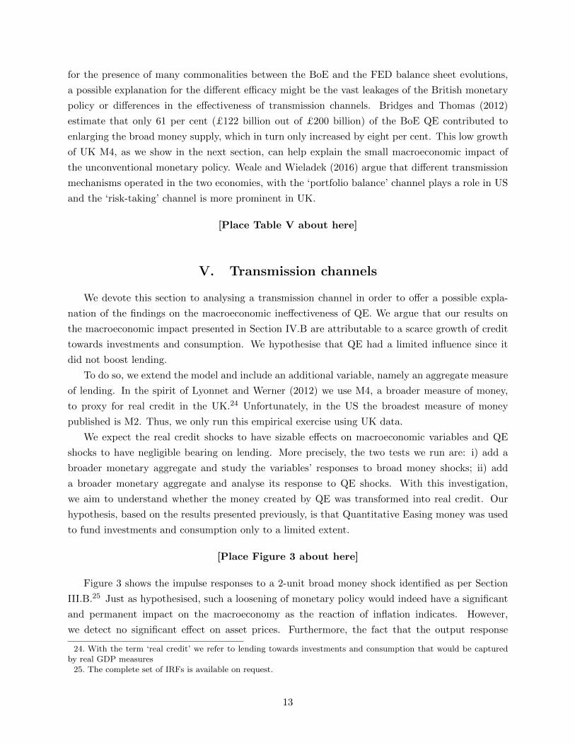
V. Transmission channels

We devote this section to analysing a transmission channel in order to offer a possible expla-

nation of the findings on the macroeconomic ineffectiveness of QE. We argue that our results on

the macroeconomic impact presented in Section IV.B are attributable to a scarce growth of credit

towards investments and consumption. We hypothesise that QE had a limited influence since it

did not boost lending.

To do so, we extend the model and include an additional variable, namely an aggregate measure

of lending. In the spirit of Lyonnet and Werner (2012) we use M4, a broader measure of money,

to proxy for real credit in the UK.24 Unfortunately, in the US the broadest measure of money

published is M2. Thus, we only run this empirical exercise using UK data.

We expect the real credit shocks to have sizable effects on macroeconomic variables and QE

shocks to have negligible bearing on lending. More precisely, the two tests we run are: i) add a

broader monetary aggregate and study the variables’ responses to broad money shocks; ii) add

a broader monetary aggregate and analyse its response to QE shocks. With this investigation,

we aim to understand whether the money created by QE was transformed into real credit. Our

hypothesis, based on the results presented previously, is that Quantitative Easing money was used

to fund investments and consumption only to a limited extent.

[Place Figure 3 about here]

Figure 3 shows the impulse responses to a 2-unit broad money shock identified as per Section

III.B.25 Just as hypothesised, such a loosening of monetary policy would indeed have a significant

and permanent impact on the macroeconomy as the reaction of inflation indicates. However,

we detect no significant effect on asset prices. Furthermore, the fact that the output response

24. With the term ‘real credit’ we refer to lending towards investments and consumption that would be capturedby real GDP measures

25. The complete set of IRFs is available on request.

13

is stable whilst price levels are boosted suggests that real credit creation in the UK supports

consumer spending more than production investment. When contrasting Figures 1 and 3 in terms

of magnitude, we note that the ratio between the size of a QE shock to the response of inflation is

around 50, whereas the proportion of the M4 shock to price levels is around 4. This means that

in order to achieve a certain inflation rate, a monetary policy aiming at increasing the size of M4

would be preferable as it would entail a much more modest enlargement of the central bank balance

sheet than a QE-like policy.

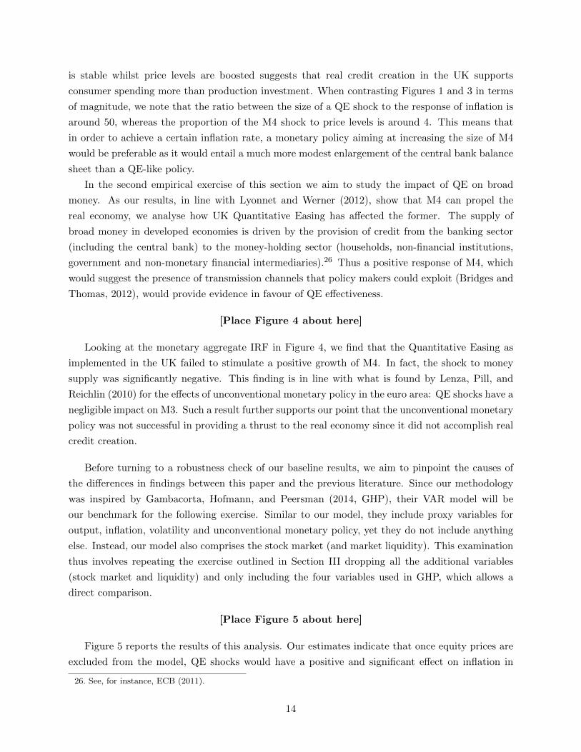
In the second empirical exercise of this section we aim to study the impact of QE on broad

money. As our results, in line with Lyonnet and Werner (2012), show that M4 can propel the

real economy, we analyse how UK Quantitative Easing has affected the former. The supply of

broad money in developed economies is driven by the provision of credit from the banking sector

(including the central bank) to the money-holding sector (households, non-financial institutions,

government and non-monetary financial intermediaries).26 Thus a positive response of M4, which

would suggest the presence of transmission channels that policy makers could exploit (Bridges and

Thomas, 2012), would provide evidence in favour of QE effectiveness.

[Place Figure 4 about here]

Looking at the monetary aggregate IRF in Figure 4, we find that the Quantitative Easing as

implemented in the UK failed to stimulate a positive growth of M4. In fact, the shock to money

supply was significantly negative. This finding is in line with what is found by Lenza, Pill, and

Reichlin (2010) for the effects of unconventional monetary policy in the euro area: QE shocks have a

negligible impact on M3. Such a result further supports our point that the unconventional monetary

policy was not successful in providing a thrust to the real economy since it did not accomplish real

credit creation.

Before turning to a robustness check of our baseline results, we aim to pinpoint the causes of

the differences in findings between this paper and the previous literature. Since our methodology

was inspired by Gambacorta, Hofmann, and Peersman (2014, GHP), their VAR model will be

our benchmark for the following exercise. Similar to our model, they include proxy variables for

output, inflation, volatility and unconventional monetary policy, yet they do not include anything

else. Instead, our model also comprises the stock market (and market liquidity). This examination

thus involves repeating the exercise outlined in Section III dropping all the additional variables

(stock market and liquidity) and only including the four variables used in GHP, which allows a

direct comparison.

[Place Figure 5 about here]

Figure 5 reports the results of this analysis. Our estimates indicate that once equity prices are

excluded from the model, QE shocks would have a positive and significant effect on inflation in

26. See, for instance, ECB (2011).

14

both countries examined. These results are qualitatively comparable to the broad money shocks

analysed in the previous section. The responses of output and volatility, instead, seem to be less

dependent on the inclusion of stocks. The omission of the stock market from the model would

lead us to similar conclusions to GHP as to the efficacy of unconventional monetary policy on the

macroeconomy.27 We thus argue that the inclusion of the stock market in assessing the impact

of unconventional monetary policy is of key importance and failing to do so can lead to biased

inferences.

Econometrically, the significance of the presence of equity prices as a link between the financial

markets and the macroeconomy in a vector autoregressive model to correctly evaluate the impact

of Quantitative Easing can be compared to the importance of: i) including indicators of financial

turmoil and uncertainty such as volatility in non-standard monetary policy VAR models to identify

an unconventional monetary policy shock (see GHP), and ii) including inflation predictors such as

commodities in standard momentary policy VAR framework to properly identify a conventional

monetary policy shock (see Christiano, Eichenbaum, and Evans, 1999).

From a theoretical view point, researchers (see for instance, Forni and Gambetti, 2014; Forni,

Gambetti, and Sala, 2014) have shown that numerous small-scale VAR models suffer from non-

fundamentalness, rendering them unable to recover true structural shocks and IRFs and unreliable

for monetary policy and business cycle analysis.28 Thus, it is plausible that small scale VARs

like the four-variable specification in GHP is non-fundamental. By adding informative and forward

looking variables such as the stock market, we may avoid the fundamentalness issue and thus better

recover structural shocks. This econometric caveat could therefore be the source of the difference

in findings and would reinforce the relevance of including the stock market in the framework.

Economically, omitting the stock market from the VAR model would be equal to disregarding

an important transmission channel, which would very possibly bias the conclusions.

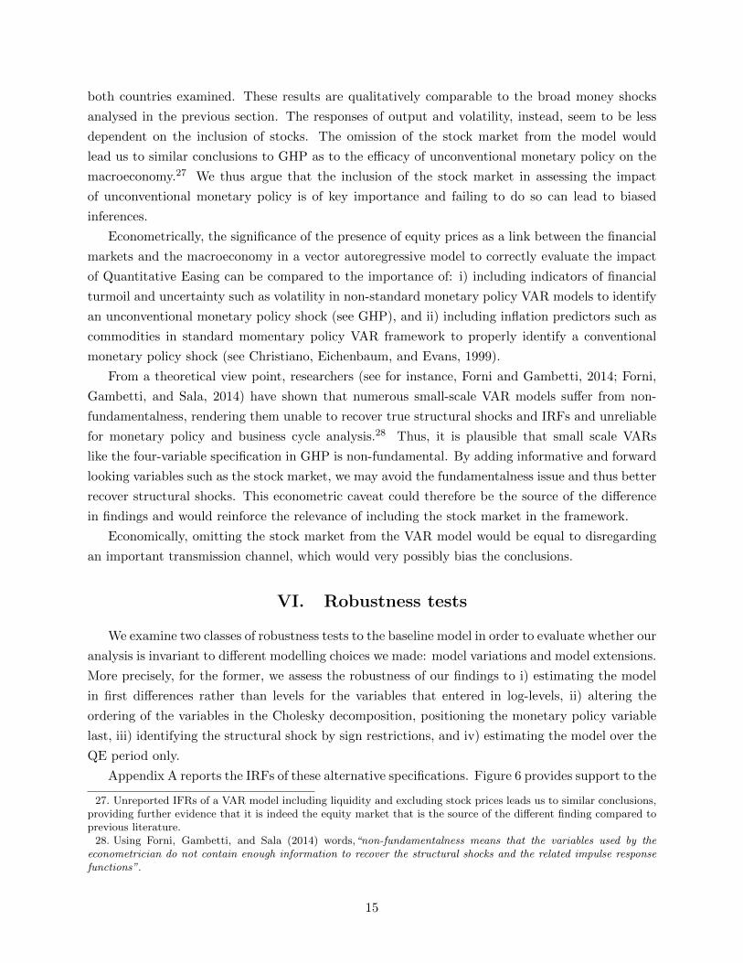
VI. Robustness tests

We examine two classes of robustness tests to the baseline model in order to evaluate whether our

analysis is invariant to different modelling choices we made: model variations and model extensions.

More precisely, for the former, we assess the robustness of our findings to i) estimating the model

in first differences rather than levels for the variables that entered in log-levels, ii) altering the

ordering of the variables in the Cholesky decomposition, positioning the monetary policy variable

last, iii) identifying the structural shock by sign restrictions, and iv) estimating the model over the

QE period only.

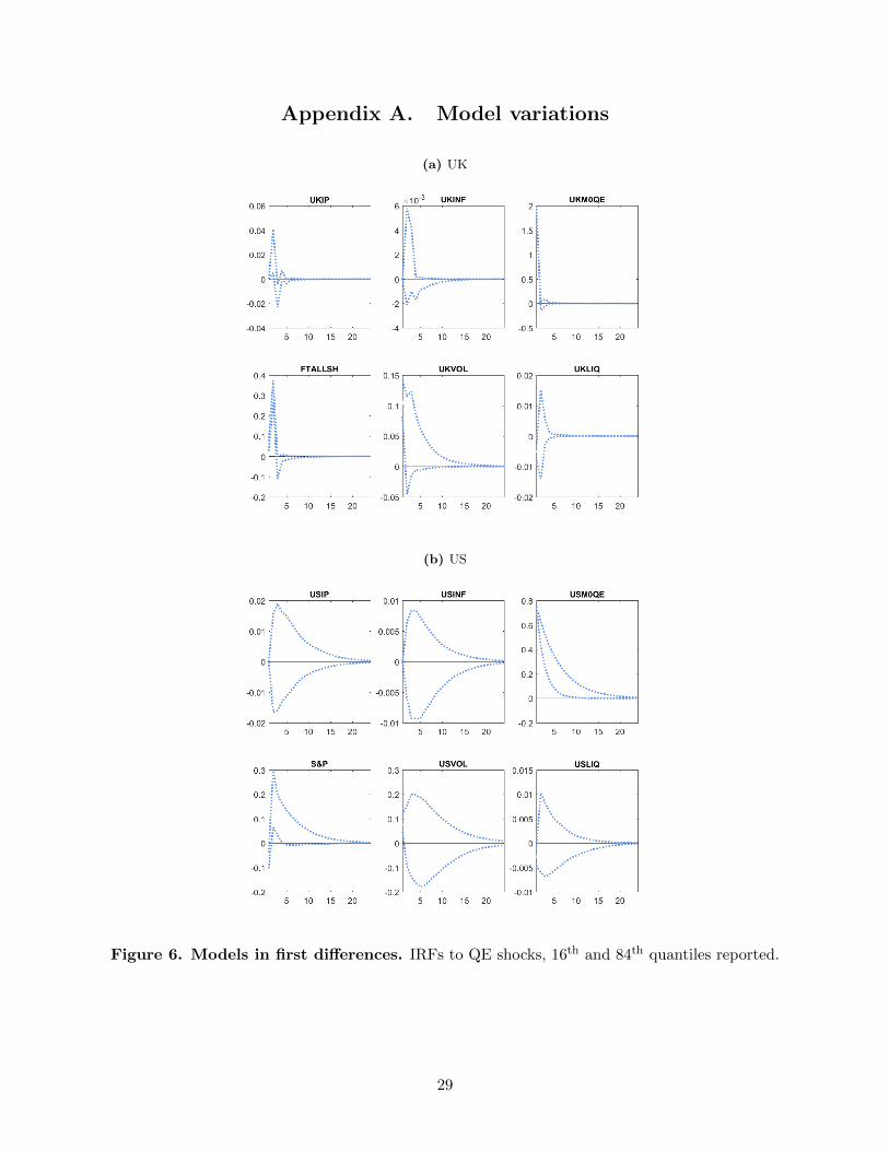
Appendix A reports the IRFs of these alternative specifications. Figure 6 provides support to the

27. Unreported IFRs of a VAR model including liquidity and excluding stock prices leads us to similar conclusions,providing further evidence that it is indeed the equity market that is the source of the different finding compared toprevious literature.

28. Using Forni, Gambetti, and Sala (2014) words,“non-fundamentalness means that the variables used by theeconometrician do not contain enough information to recover the structural shocks and the related impulse responsefunctions”.

15

qualitative robustness of our results both in direction and significance with regard to estimating the

model in (log) levels or first differences. The macroeconomic variables are not significantly affected

by the QE but the stock market level and volatility are. The effects based on the estimation in

first differences on the FTSE All-Share do not reflect the initial negative response of the baseline

model. This is perhaps the only slight difference.

Figure 7 displays the impulse responses of the alternative identification scheme. Here we restrict

all variables to respond to QE shocks with a one period delay, letting the new information carried

in the policy surprise sink into the economy and financial markets more slowly. As the main

qualitative conclusion is not altered, we find our results to be robust even to the different ‘reaction

time’ assumption.

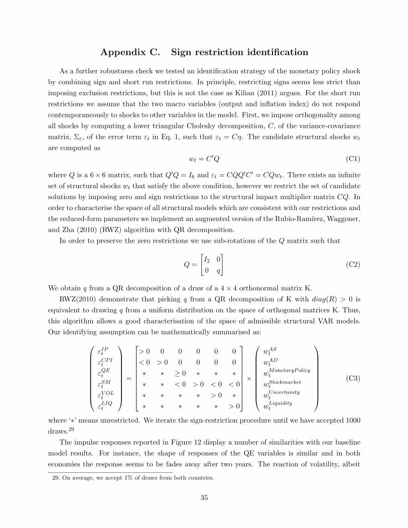
In Appendix C we describe a different approach to identifying the QE shock, achieved by sign

and zero restrictions. We constrain the contemporaneous response of macro variables to QE shocks

to zero and also allow the QE variable to respond with a one period delay, reflecting the fact that

Quantitative Easing policies were first announced and then implemented. In line with the event

study analysis of Fratzscher, Lo Duca, and Straub (2013) and Joyce et al. (2012), we restrict the

contemporaneous impact of equity prices to be negative. The response of volatility and liquidity is

left unrestricted. In order to augment the identification power of this methodology, we attempt to

identify other structural shocks. Figure 12 presents the effects of QE shocks, which are comparable

to our main findings. In both economies, output does not appear to be influenced, whereas price

levels show a modest increase in the medium term. The stock market shows a clear upward trend

after the instantaneous negative response, while volatility is reduced after about 7 to 10 months.

However, the consequences of QE for liquidity and volatility cannot be determined due to the large

standard error bands around zero.

As a final model variation we estimate a VAR model for each country over the QE period. On

the one hand, this allows us to drop M0 as a proxy to extend the QE variable time series. On

the other hand, this leaves us with around one hundred observations. We thus estimate the model

in a Bayesian fashion using the Minnesota and the sum of Coefficients priors. Estimation details

are included in Appendix D. What we find is that our baseline results are robust to this model

variation. The IRFs displayed in Figure 13 supply more evidence of little macro economic impact

of QE, and relevant positive effects on equity prices in the UK and US. Importantly, we argue that

this result jointly with low out-of-sample forecast errors over a post 2008 period, indicates that our

model is able to capture economic dynamics even at the ZLB and the results are not driven by

pre-QE observations.

We further augment the analysis of robustness by adding extra variables that might be relevant

in the analysis to our baseline model. In particular, we assess three alterations of the VAR presented

in Section III: i) an extension containing the unemployment rate, ii) an extension containing

the central bank base rate, iii) an extension containing commodity prices and, iv) an extension

containing long-term yields.

Generally, the charts presented in Appendix B, display virtually no meaningful differences

16

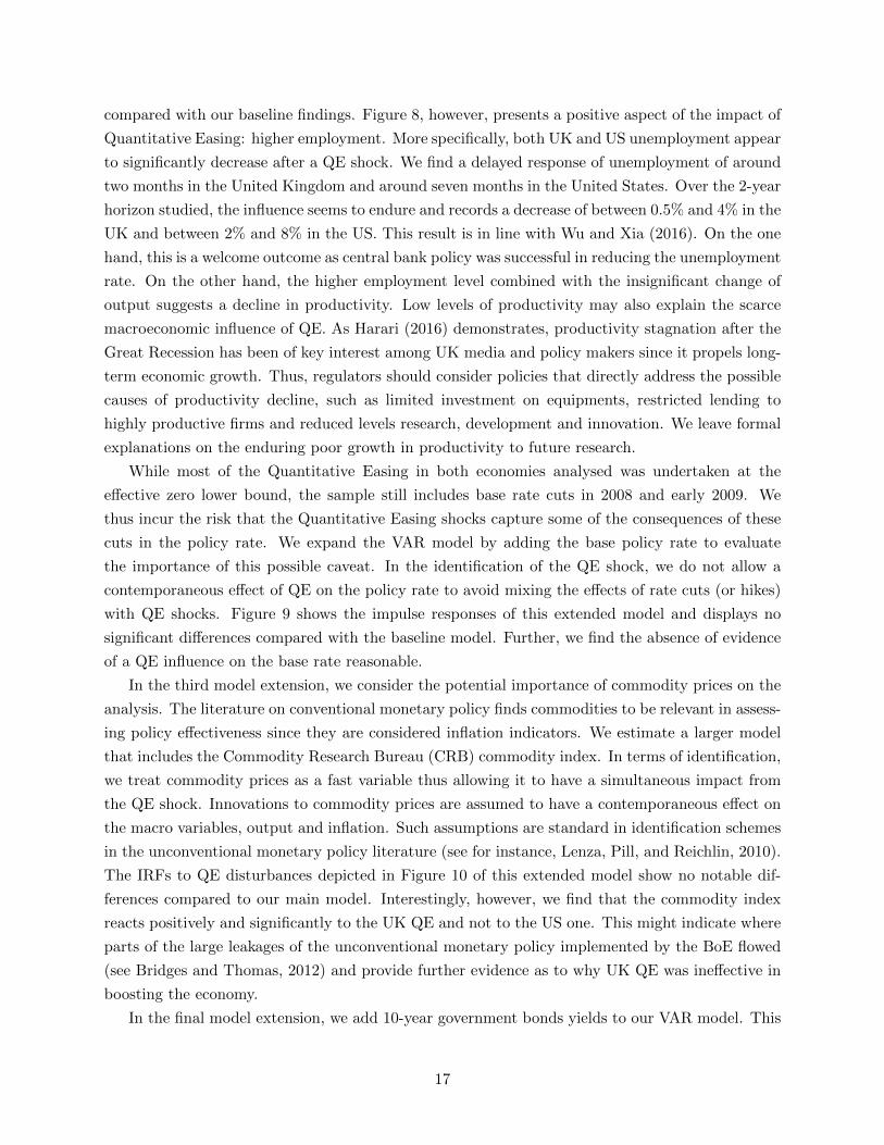
compared with our baseline findings. Figure 8, however, presents a positive aspect of the impact of

Quantitative Easing: higher employment. More specifically, both UK and US unemployment appear

to significantly decrease after a QE shock. We find a delayed response of unemployment of around

two months in the United Kingdom and around seven months in the United States. Over the 2-year

horizon studied, the influence seems to endure and records a decrease of between 0.5% and 4% in the

UK and between 2% and 8% in the US. This result is in line with Wu and Xia (2016). On the one

hand, this is a welcome outcome as central bank policy was successful in reducing the unemployment

rate. On the other hand, the higher employment level combined with the insignificant change of

output suggests a decline in productivity. Low levels of productivity may also explain the scarce

macroeconomic influence of QE. As Harari (2016) demonstrates, productivity stagnation after the

Great Recession has been of key interest among UK media and policy makers since it propels long-

term economic growth. Thus, regulators should consider policies that directly address the possible

causes of productivity decline, such as limited investment on equipments, restricted lending to

highly productive firms and reduced levels research, development and innovation. We leave formal

explanations on the enduring poor growth in productivity to future research.

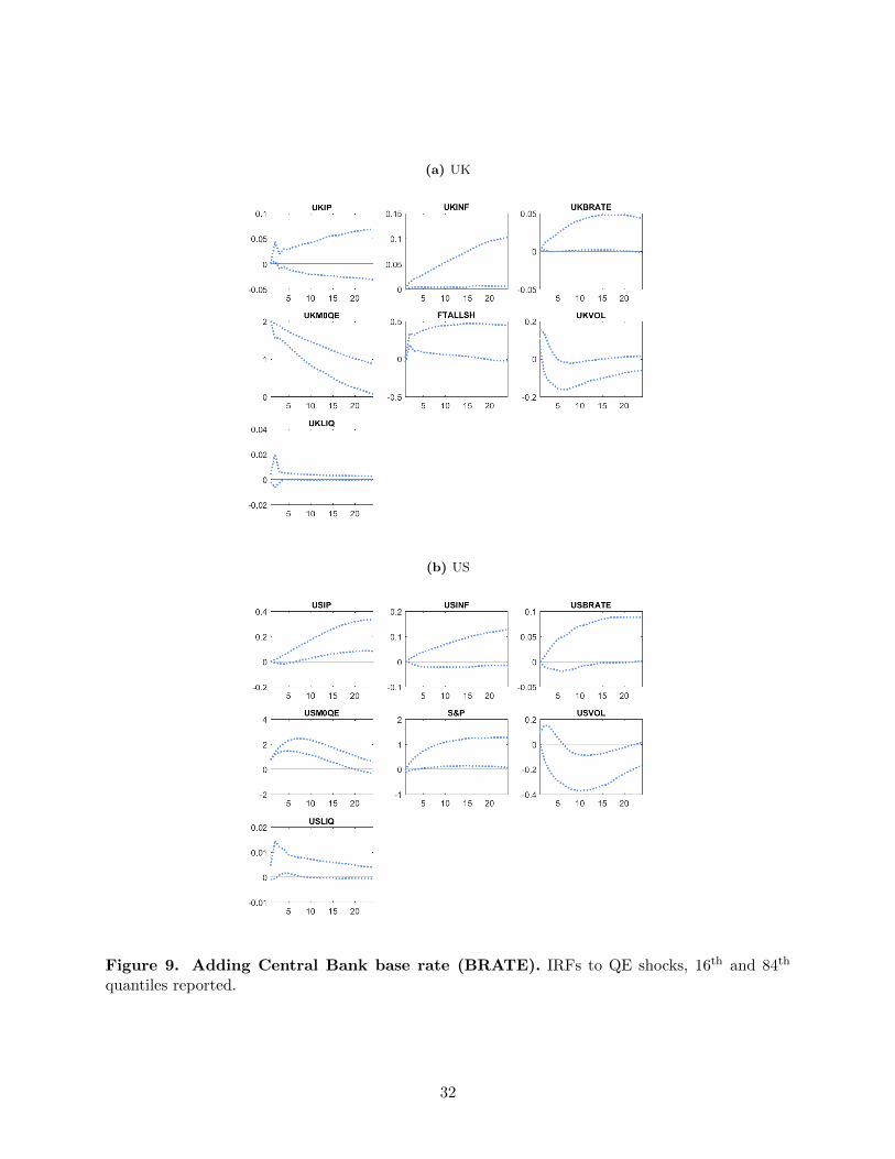
While most of the Quantitative Easing in both economies analysed was undertaken at the

effective zero lower bound, the sample still includes base rate cuts in 2008 and early 2009. We

thus incur the risk that the Quantitative Easing shocks capture some of the consequences of these

cuts in the policy rate. We expand the VAR model by adding the base policy rate to evaluate

the importance of this possible caveat. In the identification of the QE shock, we do not allow a

contemporaneous effect of QE on the policy rate to avoid mixing the effects of rate cuts (or hikes)

with QE shocks. Figure 9 shows the impulse responses of this extended model and displays no

significant differences compared with the baseline model. Further, we find the absence of evidence

of a QE influence on the base rate reasonable.

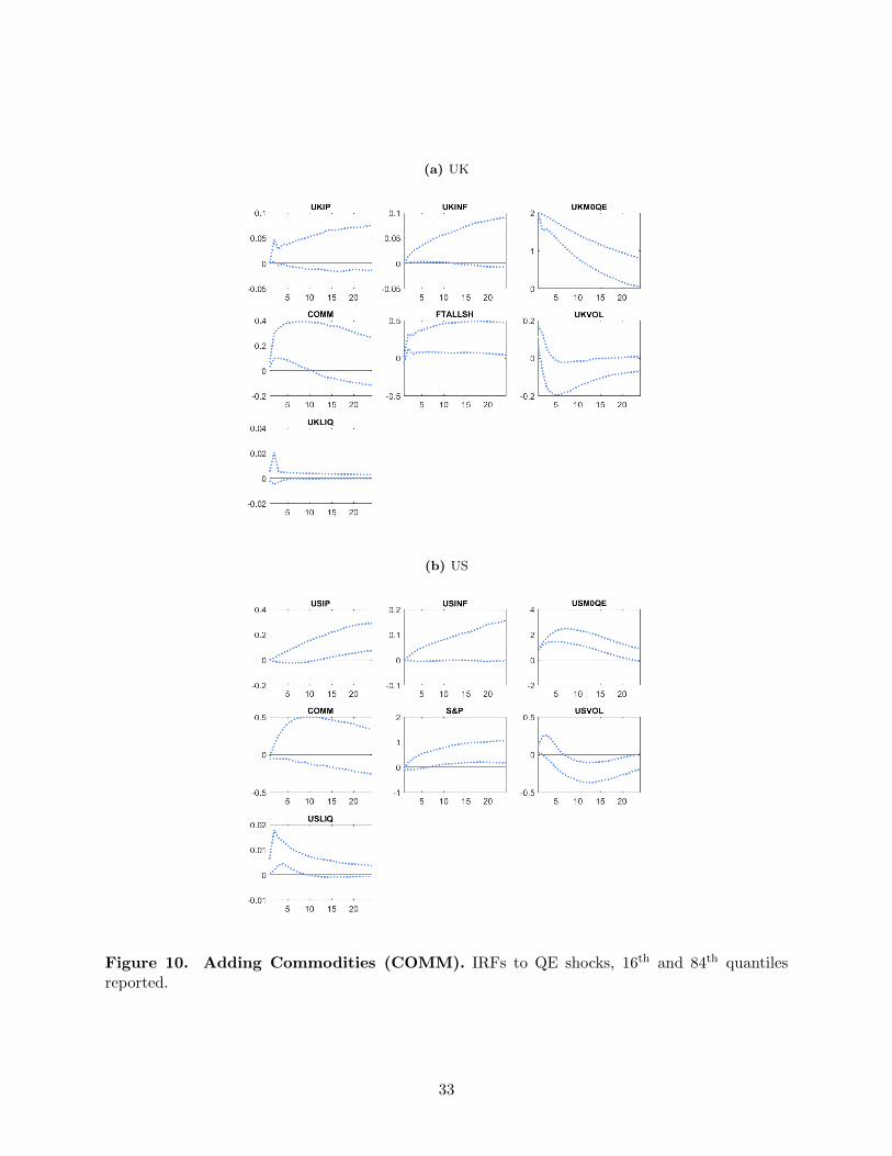
In the third model extension, we consider the potential importance of commodity prices on the

analysis. The literature on conventional monetary policy finds commodities to be relevant in assess-

ing policy effectiveness since they are considered inflation indicators. We estimate a larger model

that includes the Commodity Research Bureau (CRB) commodity index. In terms of identification,

we treat commodity prices as a fast variable thus allowing it to have a simultaneous impact from

the QE shock. Innovations to commodity prices are assumed to have a contemporaneous effect on

the macro variables, output and inflation. Such assumptions are standard in identification schemes

in the unconventional monetary policy literature (see for instance, Lenza, Pill, and Reichlin, 2010).

The IRFs to QE disturbances depicted in Figure 10 of this extended model show no notable dif-

ferences compared to our main model. Interestingly, however, we find that the commodity index

reacts positively and significantly to the UK QE and not to the US one. This might indicate where

parts of the large leakages of the unconventional monetary policy implemented by the BoE flowed

(see Bridges and Thomas, 2012) and provide further evidence as to why UK QE was ineffective in

boosting the economy.

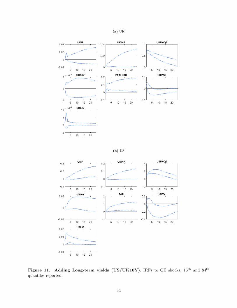
In the final model extension, we add 10-year government bonds yields to our VAR model. This

17

variable represents a key channel of transmission of the unconventional monetary policy since QE

is supposed to operate by lowering long-term interest rates. For this exercise, we use the short-run

identification scheme employed in the baseline model. In terms of Cholesky ordering, we place 10-

year yields among the fast moving variables, just below QE, in order to allow a contemporaneous

impact of a QE shock on bond prices. Turning to the results, for the US model, Figure 11 shows a

significant decrease in long-term interest rates contemporaneous to the QE shock, that fades away

thereafter. This is a common result the literature (see for instance, Krishnamurthy and Vissing-

Jorgensen, 2011; Gagnon et al., 2011; D’Amico and King, 2013). The responses of the other US

macro and financial variables is qualitatively similar to our findings in Section IV. For the UK, we

also find that our results are robust to the addition of long-term government bonds. However, there

exist a difference between the US and UK impulse responses depicted in Figure 11, since 10-year

UK yields show no significant decline after an unconventional monetary policy shock.

VII. Conclusions

This paper is an empirical study of the effectiveness of the Quantitative Easing programme

implemented by the Bank of England and the Federal Reserve Bank to tackle the Great Recession.

We conduct an econometric analysis based on a six-variable VAR model, which we develop for

each of the two countries. The models jointly include macro variables – output, inflation, QE

amounts – and financial markets variables – equity prices, stock market volatility and liquidity.

Thanks to this comprehensive framework, not only are we able to study various influences of the

monetary stimulus on stock markets, but also find the inclusion of financial measures relevant in

policy assessment studies. Unlike other studies (e.g. Kapetanios et al., 2012; Pesaran and Smith,

2012), our framework does not rely on the impact estimates of the yield curve and its linkages

with the stock markets. On the contrary, QE enters in our model directly as a variable on its

own, thereby allowing for other possible transmission channels. Before turning to estimating the

impact of unconventional monetary policy, we run a model validation analysis based on comparing

the forecasting power of our base line model with the random walk benchmark. The results of

this validation exercise jointly with the model estimates provide evidence that the model usefully

captures the dynamic relationships between variables, indicating the adequacy of the model for the

scope of our research.

In order to assess the effects of QE, we compute the impulse response functions of the variables

included in the models to QE shocks. We find that exogenous QE shocks only have a meaningful

impact on financial variables. More specifically, the estimates suggest no significant effects on UK

output and inflation and US price levels, whereas US output only increases significantly with a

12-month lag.

The analysis demonstrates some differences in the domestic effectiveness of the unconventional

policies undertaken in the US and UK. The FED actions appear to have had a greater influence

than those of the BoE, perhaps due to the large leakages of the money injected in Britain, which

18

is a small open economy.

The two economies’ stock market reactions are found to be ‘V’ shaped: markets respond ad-

versely in the few months following the announcement but subsequently regain the losses and

increase even further. Stock market volatility paints the opposite picture as it displays a positive

reaction following a QE shock before it becomes negative. Finally, our findings show a different

reaction between US and UK stock market liquidity since we find that the former is negatively

affected whereas the latter remains virtually unaltered. Our estimates formally lend support to the

widespread belief that Quantitative Easing in the United States and in the United Kingdom had a

considerable positive influence on equity prices.

These results are qualitatively similar to those in some of the previous literature (e.g. Lyonnet

and Werner, 2012) but contrast with other papers (e.g. Gambacorta, Hofmann, and Peersman,

2014), especially in terms of the macroeconomic impact. We conduct a further empirical exercise

which explores the source of the differences, and find that the inclusion of the stock market in VAR

models to assess the impact of unconventional monetary policy is of key importance. This result

provides econometric backing to the possible non-fundamentalness of the small scale VAR models

used in some of the previous literature. More precisely, we argue that the expansion of the central

bank balance sheet was not channelled into credit creation for investments and consumption. The

consequence of this was an evident increase in equity prices not followed by an improvement in the

macroeconomic outlook.

In summary, our findings supply evidence on the limitations of ‘unconstrained’ Quantitative

Easing, in addition to the massive central bank balance sheet expansion required in the process.

Should policy makers intend to undertake new QE rounds, we argue that such measures need to be

combined with ‘constraining’ policies aimed at channelling the monetary stimulus into lending that

boost consumption and investments, rather than into financial assets. In other words, monetary

policy targeting the size of larger monetary aggregates, such as M4, rather than the monetary base,

should be preferable.

19

References

Banbura, Marta, Domenico Giannone, and Lucrezia Reichlin. 2010. “Large Bayesian Vector Auto

Regressions.” Journal of Applied Econometrics 25, no. 1 (January): 71–92.

Bernanke, Ben. 2009. “The Federal Reserve’s Balance Sheet: An Update.” In Speech at the Federal

Reserve Board Conference on Key Developments in Monetary Policy, Washington, DC, vol. 8.

Bernanke, Ben, Jean Boivin, and Piotr Eliasz. 2005. “Measuring the Effects of Monetary Policy:

A Factor-Augmented Vector Autoregressive (FAVAR) Approach.” The Quarterly Journal of

Economics 120 (1): 387–422.

Bhattarai, Saroj, Arpita Chatterjee, and Woong Yong Park. 2015. Effects of US Quantitative Eas-

ing on Emerging Market Economies. Discussion Paper 2015-26. School of Economics, The

University of New South Wales.

Bjørnland, Hilde C., and Kai Leitemo. 2009. “Identifying the Interdependence between US Mone-

tary Policy and the Stock Market.” Journal of Monetary Economics 56 (2): 275–282.

Breedon, F., J. S. Chadha, and A. Waters. 2012. “The Financial Market Impact of UK Quantitative

Easing.” Oxford Review of Economic Policy 28, no. 4 (December): 702–728.

Bridges, Jonathan, and Ryland Thomas. 2012. The Impact of QE on the UK Economy–some Sup-

portive Monetarist Arithmetic. Bank of England working paper 442. Bank of England.

Butt, Nicholas, Silvia Domit, Michael McLeay, Ryland Thomas, and Lewis Kirkham. 2012. “What

Can the Money Data Tell Us about the Impact of QE?” Bank of England Quarterly Bulletin

52 (4): 321–331.

Cesa-Bianchi, Ambrogio, Gregory Thwaites, and Alejandro Vicondoa. 2016. Monetary Policy Trans-

mission in an Open Economy: New Data and Evidence from the United Kingdom. Discussion

Paper 1612. Centre for Macroeconomics (CFM).

Christiano, Lawrence J., Martin Eichenbaum, and Charles L. Evans. 1999. “Monetary Policy

Shocks: What Have We Learned and to What End?” In Handbook of Macroeconomics, 65–

148. Elsevier.

D’Amico, Stefania, and Thomas B. King. 2013. “Flow and Stock Effects of Large-Scale Treasury

Purchases: Evidence on the Importance of Local Supply.” Journal of Financial Economics 108

(2): 425–448.

Dudley, William. 2010. “The Outlook, Policy Choices and Our Mandate.” Remarks at the Society

of American Business Editors and Writers Fall Conference, City University of New York.

ECB. 2011. “The Supply of Money – Bank Behaviour and the Implications for Monetary Analysis.”

Monthly Bulletin (October).

20

Eggertsson, Gauti B., and Michael Woodford. 2003. “Zero Bound on Interest Rates and Optimal

Monetary Policy.” Brookings Papers on Economic Activity 2003 (1): 139–233.

Eickmeier, Sandra, and Boris Hofmann. 2013. “Monetary Policy, Housing Booms, and Financial

(Im)balances.” Macroeconomic Dynamics 17, no. 04 (June): 830–860.

Engen, Eric M., Thomas Laubach, and Dave Reifschneider. 2015. The Macroeconomic Effects of

the Federal Reserve’s Unconventional Monetary Policies. Technical report. Washington: Board

of Governors of the Federal Reserve System.

Forni, Mario, and Luca Gambetti. 2014. “Sufficient Information in Structural VARs.” Journal of

Monetary Economics 66:124–136.

Forni, Mario, Luca Gambetti, and Luca Sala. 2014. “No News in Business Cycles.” The Economic

Journal 124 (581): 1168–1191.

Fratzscher, Marcel, Marco Lo Duca, and Roland Straub. 2013. On the International Spillovers of

US Quantitative Easing. Discussion Papers of DIW Berlin 1304. DIW Berlin, German Institute

for Economic Research.

Gagnon, Joseph, Matthew Raskin, Julie Remache, Brian Sack, et al. 2011. “The Financial Market

Effects of the Federal Reserve’s Large-Scale Asset Purchases.” International Journal of Central

Banking 7 (1): 3–43.

Gagnon, Joseph, Matthew Raskin, Julie Remache, and Brian P. Sack. 2010. “Large-Scale Asset

Purchases by the Federal Reserve: Did They Work?” FRB of New York Staff Report, no. 441.

Gambacorta, Leonardo, Boris Hofmann, and Gert Peersman. 2014. “The Effectiveness of Uncon-

ventional Monetary Policy at the Zero Lower Bound: A Cross-Country Analysis.” Journal of

Money, Credit and Banking 46, no. 4 (June): 615–642.

Giannone, Domenico, Michele Lenza, and Giorgio E. Primiceri. 2015. “Prior Selection for Vector

Autoregressions.” Review of Economics and Statistics 97 (2): 436–451.

Giannone, Domenico, Michele Lenza, and Lucrezia Reichlin. 2014. Money, Credit, Monetary Policy

and the Business Cycle in the Euro Area: What Has Changed since the Crisis. Technical report.

ECB mimeo.

Goyenko, Ruslan Y., Craig W. Holden, and Charles A. Trzcinka. 2009. “Do Liquidity Measures

Measure Liquidity?” Journal of financial Economics 92 (2): 153–181.

Hamilton, James D., and Jing Cynthia Wu. 2012. “The Effectiveness of Alternative Monetary Policy

Tools in a Zero Lower Bound Environment.” Journal of Money, Credit and Banking 44 (s1):

3–46.

Hancock, Diana, and Wayne Passmore. 2011. “Did the Federal Reserve’s MBS Purchase Program

Lower Mortgage Rates?” Journal of Monetary Economics 58 (5): 498–514.

21

Harari, Daniel. 2016. “Productivity in the UK.” House of Commons Library Briefing Paper, no.

Number 06492 (November).

Joyce, Michael, Ana Lasaosa, Ibrahim Stevens, and Matthew Tong. 2011. “The Financial Mar-

ket Impact of Quantitative Easing in the United Kingdom.” International Journal of Central

Banking 7 (3): 113–161.

Joyce, Michael, David Miles, Andrew Scott, and Dimitri Vayanos. 2012. “Quantitative Easing and

Unconventional Monetary Policy–an Introduction*.” The Economic Journal 122 (564): F271–

F288.

Kapetanios, George, Haroon Mumtaz, Ibrahim Stevens, and Konstantinos Theodoridis. 2012. “As-

sessing the Economy-Wide Effects of Quantitative Easing*.” The Economic Journal 122 (564):

F316–F347.

Kilian, Lutz. 2011. Structural Vector Autoregressions. CEPR Discussion Paper 8515. C.E.P.R. Dis-

cussion Papers.

Krishnamurthy, Arvind, and Annette Vissing-Jorgensen. 2011. “The Effects of Quantitative Eas-

ing on Interest Rates: Channels and Implications for Policy.” Brookings Papers on Economic

Activity Fall:215–265.

Lenza, Michele, Huw Pill, and Lucrezia Reichlin. 2010. “Monetary Policy in Exceptional Times.”

Economic Policy 25 (62): 295–339.

Lyonnet, Victor, and Richard Werner. 2012. “Lessons from the Bank of England on ‘quantitative

Easing’ and Other ‘unconventional’ Monetary Policies.” International Review of Financial

Analysis, Banking and the Economy, 25 (December): 94–105.

Mankiw, N. Gregory, and Ricardo Reis. 2002. “Sticky Information versus Sticky Prices: A Proposal

to Replace the New Keynesian Phillips Curve.” The Quarterly Journal of Economics 117, no.

4 (January): 1295–1328.

McCallum, Bennett T. 2000. “Theoretical Analysis Regarding a Zero Lower Bound on Nominal

Interest Rates.” Journal of Money, Credit and Banking 32 (4): 870–904.

Neely, Christopher J. 2010. The Large Scale Asset Purchases Had Large International Effects.

Federal Reserve Bank of St. Louis, Research Division.

Pesaran, M. Hashem, and Ron Smith. 2012. Counterfactual Analysis in Macroeconometrics: An

Empirical Investigation into the Effects of Quantitative Easing. IZA Discussion Paper 6618.

Institute for the Study of Labor (IZA).

Rogers, John H., Chiara Scotti, and Jonathan H. Wright. 2014. “Evaluating Asset-Market Effects

of Unconventional Monetary Policy: A Multi-Country Review.” Economic Policy 29 (80): 749–

799.

22

Roll, Richard. 1984. “A Simple Implicit Measure of the Effective Bid-Ask Spread in an Efficient

Market.” The Journal of Finance 39, no. 4 (September): 1127–1139.

Rubio-Ramırez, Juan F., Daniel F. Waggoner, and Tao Zha. 2010. “Structural Vector Autoregres-

sions: Theory of Identification and Algorithms for Inference.” The Review of Economic Studies

77, no. 2 (January): 665–696.

Shiller, Robert J. 1981. “Do Stock Prices Move Too Much to Be Justified by Subsequent Changes

in Dividends?” The American Economic Review 71 (3): 421–436.

Sims, Christopher A., James H. Stock, and Mark W. Watson. 1990. “Inference in Linear Time

Series Models with Some Unit Roots.” Econometrica 58 (1): 113–144.

Voutsinas, Konstantinos, and Richard A. Werner. 2010. New Evidence on the Effectiveness of ‘quan-

titative Easing’ and the Accountability of the Central Bank in Japan. Technical report. Working

paper presented at the 15th Annual Meeting of the Annual International Conference on Macroe-

conomic Analysis and International Finance (ICMAIF 2011), University of Crete, Rethymnon,

27 May 2011.

Weale, Martin, and Tomasz Wieladek. 2016. “What Are the Macroeconomic Effects of Asset Pur-

chases?” Journal of Monetary Economics 79 (May): 81–93.

Werner, Richard A. 2012. “Towards a New Research Programme on ‘banking and the Economy’ —

Implications of the Quantity Theory of Credit for the Prevention and Resolution of Banking

and Debt Crises.” International Review of Financial Analysis, Banking and the Economy, 25

(December): 1–17.

Williams, John C. 2016. Monetary Policy in a Low R-Star World. Federal Reserve Bank of San

Francisco Economic Letters.

Wu, C. F. J. 1986. “Jackknife, Bootstrap and Other Resampling Methods in Regression Analysis.”

The Annals of Statistics 14 (4): 1261–1295.

Wu, Jing Cynthia, and Fan Dora Xia. 2016. “Measuring the Macroeconomic Impact of Monetary

Policy at the Zero Lower Bound.” Journal of Money, Credit and Banking 48, nos. 2-3 (March):

253–291.

Yellen, Janet. 2015. “The Outlook for the Economy.” Speech At the Providence Chamber of Com-

merce, Providence, Rhode Island (May).

23

Tables and Figures

Table I

Mnemonics Variable Description Source Levels Slow/Fast

UKIP Output UK industrial production DS Log-levels SUKINF Inflation UK RPI DS Log-levels SUKM0QE UK QE UK M0 & UK QE DS Log-levels PolicyFTALLSH Stock Market FTSE All-Share DS Log-levels FUKVOL Stock Market Volatility FTALLSH 30-day StDev OC Levels/100 FUKLIQ Stock Market Liquidity Roll(1984) bid-ask spread OC Levels/100 F

UK dataset. The data sources are Datastream (DS) and authors own calculation (OC).

Table II

Mnemonics Variable Description Source Levels Slow/Fast

USIP Output US industrial production DS Log-levels SUSINF Inflation US CPI DS Log-levels SUSM0QE US QE US M0 & US QE FR Log-levels PolicyFTALLSH Stock Market S&P 500 DS Log-levels FUSVOL Stock Market Volatility S&P 500 30-day StDev OC Levels/100 FUSLIQ Stock Market Liquidity Roll(1984) bid-ask spread OC Levels/100 F

US dataset. The data sources are Datastream (DS), FRED (FR) and authors own calculation(OC).

24

Table III

Horizon Variables VAR RW Theil’s-U

1M UKIP 0.007 0.010 0.77UKINF 0.007 0.004 1.72UKM0QE 0.053 0.043 1.23FTALLSH 0.042 0.034 1.24UKVOL 0.039 0.034 1.15UKLIQ 0.004 0.005 0.75

3M UKIP 0.010 0.012 0.86UKINF 0.009 0.008 1.18UKM0QE 0.077 0.078 0.98FTALLSH 0.035 0.049 0.71UKVOL 0.048 0.058 0.83UKLIQ 0.004 0.006 0.67

UK Out-of-sample forecasting errors.

Table IV

Horizon Variables VAR RW Theil’s-U

1M USIP 0.009 0.004 2.18USINF 0.004 0.002 1.74USM0QE 0.031 0.018 1.70S&P 0.050 0.040 1.24USVOL 0.043 0.039 1.10USLIQ 0.002 0.004 0.59

3M USIP 0.016 0.009 1.79USINF 0.005 0.005 0.92USM0QE 0.013 0.054 0.24S&P 0.054 0.063 0.85USVOL 0.030 0.066 0.46USLIQ 0.003 0.004 0.82

US Out-of-sample forecasting errors.

Table V

Short-run effect Long-run effect

UK Output Briefly positive Insignificant effectInflation Insignificant effect Insignificant effectStock market Negative on impact PositiveVolatility Positive NegativeLiquidity Negative Insignificant effect

US Output Insignificant effect PositiveInflation Insignificant effect Insignificant effectStock market Negative on impact PositiveVolatility Positive NegativeLiquidity Negative Insignificant effect

Summary of main findings. Short and long-run effects of QE shocks.

25

Figure 1. UK baseline model Impulse response functions. IRFs to QE shocks, 16th and84th quantiles reported.

Figure 2. US baseline model Impulse response functions. IRFs to QE shocks, 16th and84th quantiles reported.

26

Figure 3. UK extended model Impulse response functions. IRFs to broad money (M4)shocks, 16th and 84th quantiles reported.

Figure 4. UK extended model Impulse response functions. IRFs to QE shocks, 16th and84th quantiles reported.

27

(a) UK

(b) US

Figure 5. Reduced models Impulse response functions. IRFs to QE shocks, 16th and 84th

quantiles reported.

28

Appendix A. Model variations

(a) UK

(b) US

Figure 6. Models in first differences. IRFs to QE shocks, 16th and 84th quantiles reported.

29

(a) UK

(b) US

Figure 7. Altered cholesky ordering. IRFs to QE shocks, 16th and 84th quantiles reported.

30

Appendix B. Model extensions

(a) UK

(b) US

Figure 8. Adding unemployment. IRFs to QE shocks, 16th and 84th quantiles reported.

31

(a) UK

(b) US

Figure 9. Adding Central Bank base rate (BRATE). IRFs to QE shocks, 16th and 84th

quantiles reported.

32

(a) UK

(b) US

Figure 10. Adding Commodities (COMM). IRFs to QE shocks, 16th and 84th quantilesreported.

33

(a) UK

(b) US

Figure 11. Adding Long-term yields (US/UK10Y). IRFs to QE shocks, 16th and 84th

quantiles reported.

34

Appendix C. Sign restriction identification

As a further robustness check we tested an identification strategy of the monetary policy shock

by combining sign and short run restrictions. In principle, restricting signs seems less strict than

imposing exclusion restrictions, but this is not the case as Kilian (2011) argues. For the short run

restrictions we assume that the two macro variables (output and inflation index) do not respond

contemporaneously to shocks to other variables in the model. First, we impose orthogonality among

all shocks by computing a lower triangular Cholesky decomposition, C, of the variance-covariance

matrix, Σε, of the error term εt in Eq. 1, such that εt = Cη. The candidate structural shocks wt

are computed as

wt = C ′Q (C1)

where Q is a 6× 6 matrix, such that Q′Q = I6 and εt = CQQ′C ′ = CQwt. There exists an infinite

set of structural shocks wt that satisfy the above condition, however we restrict the set of candidate

solutions by imposing zero and sign restrictions to the structural impact multiplier matrix CQ. In

order to characterise the space of all structural models which are consistent with our restrictions and

the reduced-form parameters we implement an augmented version of the Rubio-Ramırez, Waggoner,

and Zha (2010) (RWZ) algorithm with QR decomposition.

In order to preserve the zero restrictions we use sub-rotations of the Q matrix such that

Q =

[I2 0

0 q

](C2)

We obtain q from a QR decomposition of a draw of a 4× 4 orthonormal matrix K.

RWZ(2010) demonstrate that picking q from a QR decomposition of K with diag(R) > 0 is

equivalent to drawing q from a uniform distribution on the space of orthogonal matrices K. Thus,

this algorithm allows a good characterisation of the space of admissible structural VAR models.

Our identifying assumption can be mathematically summarised as:

εIPt

εCPIt

εQEtεSMt

εV OLt

εLIQt

=

> 0 0 0 0 0 0

< 0 > 0 0 0 0 0

∗ ∗ ≥ 0 ∗ ∗ ∗∗ ∗ < 0 > 0 < 0 < 0

∗ ∗ ∗ ∗ > 0 ∗∗ ∗ ∗ ∗ ∗ > 0

×

wASt

wADt

wMonetaryPolicyt

wStockmarkett

wUncertaintyt

wLiquidityt

(C3)

where ‘∗’ means unrestricted. We iterate the sign-restriction procedure until we have accepted 1000

draws.29

The impulse responses reported in Figure 12 display a number of similarities with our baseline

model results. For instance, the shape of responses of the QE variables is similar and in both

economies the response seems to be fades away after two years. The reaction of volatility, albeit

29. On average, we accept 1% of draws from both countries.

35

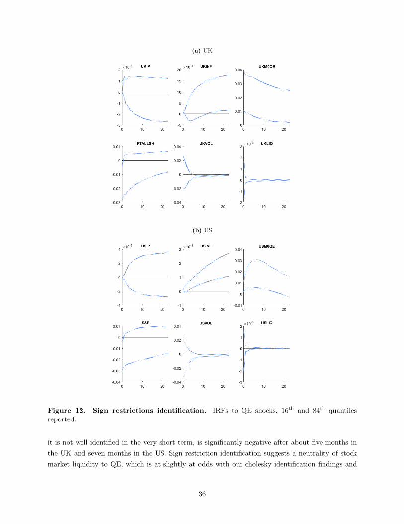
(a) UK

(b) US

Figure 12. Sign restrictions identification. IRFs to QE shocks, 16th and 84th quantilesreported.

it is not well identified in the very short term, is significantly negative after about five months in

the UK and seven months in the US. Sign restriction identification suggests a neutrality of stock

market liquidity to QE, which is at slightly at odds with our cholesky identification findings and

36

with the literature on bond market liquidity. Lastly, moving to the macroeconomic analysis, our

main conclusions on the neutrality of QE on output are strengthened as the error bands of the

responses of industrial production are centred around zero. However, Figure 12 presents some

evidence on a positive effect of inflation following a QE shock, starting in the very short term for

the US and after around one year in the UK.

37

Appendix D. Monetary aggregates and QE

Since we are extending the time series of securities held outright by the two central banks with

the respective measures of M0, we want to rule out the possibility that our findings are driven by

this proxy.

Firstly, we note that, for the US, the correlation between the variable QE and M0 for the

overlapping period (2006-2015) is 0.98. For the UK, the correlation between the QE amount and

M0 (over the 2009-2015 period) is 0.86. BoE total assets have a larger overlapping span since the

monthly data start in 2006 and their correlation with M0 is 0.97. These figures close to unity

indicate that the assets held at the central banks comove significantly with M0.

Secondly, we can re-estimate the VAR model only over the period for which we have data on

QE amounts available. Given the drastically lower number of observations in this scenario, we

estimate a BVAR model with Minnesota and sum of coefficients (SOC) prior.

We choose conjugate prior distributions of the VAR coefficients that belong to the following Normal-

Inverse-Wishart family:

β|Σ ∼ N(b,Σ⊗ Ω)

Σ ∼ IW (Ψ, d)(D1)

where b,Ω,Ψ and d are the prior parameters. The Minnesota prior has the following first and

second moments:

E[(Bs)ij |Σ] =

δi if i = j and s = 1

0 otherwise

cov[(Bs)ij , (Br)hm|Σ] =

λ2

s2Σih

ψ/(d−n−1) if m = j and r = s

0 otherwise

δi is set to 1 for variables believed to be highly persistent (the ones we express in log-levels) and

set to 0 for those believed to mean revert. The prior on the intercept is diffuse. The hyperparameter

λ dermines the overall tightness of the prior and is set equal to 0.2. For the SOC prior we construct

the following matrices of dummy observations:

Y +

n×n= diag

(Y0

µ

)X+

n×(1+np)=

[0n×1

, Y +, ..., Y +

]where Y0 is an n× 1 vector of averages of the first p observations and the hyperparameter µ is

set to 1.

For internal consistency, we plot the 16th and 84th percentiles of the impulse responses densities

38

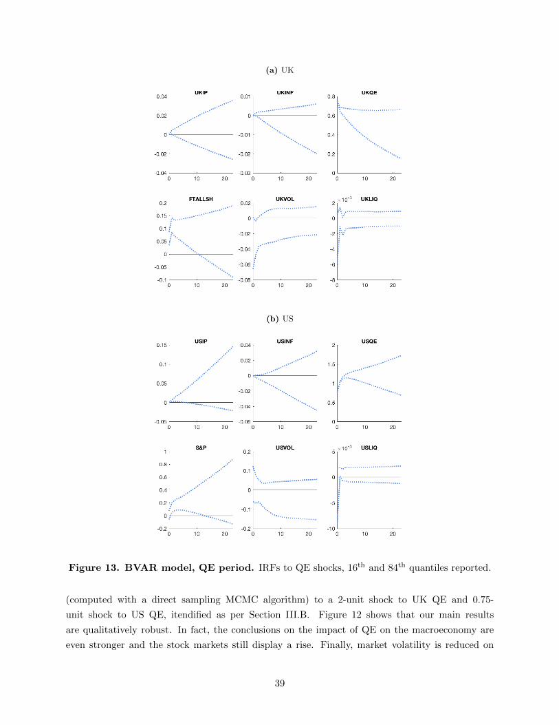
(a) UK

(b) US

Figure 13. BVAR model, QE period. IRFs to QE shocks, 16th and 84th quantiles reported.

(computed with a direct sampling MCMC algorithm) to a 2-unit shock to UK QE and 0.75-

unit shock to US QE, itendified as per Section III.B. Figure 12 shows that our main results

are qualitatively robust. In fact, the conclusions on the impact of QE on the macroeconomy are

even stronger and the stock markets still display a rise. Finally, market volatility is reduced on

39

impact in the UK and only after 3 to 4 months in the US whereas (il)liquidity shows a negative

contemporaneous response to the QE shock.

40