1

DICE 2013R: Introduction and User’s Manual

William Nordhaus

with

Paul Sztorc

Second edition

October 2013

Copyright William Nordhaus 2013

First edition: April 2013

Website: dicemodel.net

2

Table of Contents (New materials are with *)

I. Preface (*) ................................................................................................................... 3

II. DICE and RICE Models as Integrated Assessment Models ............................... 4

A. Introduction to the models ..................................................................................... 4

B. Objectives of Integrated Assessment Models (IAMs) ......................................... 5

III. Detailed Equations of the DICE-2013R Model ................................................... 6

A. Preferences and the Objective Function ............................................................... 6

B. Economic Variables .................................................................................................. 8

C. Geophysical sectors ............................................................................................... 15

D. The RICE-2010 Model ........................................................................................... 19

E. Interpretation of Positive and Normative Models (*) ....................................... 21

F. Consistency with the IPCC Fifth Assessment Report (*) .................................. 22

IV. Results from the DICE-2013R Model (*) .......................................................... 24

A. Scenarios ................................................................................................................. 24

B. Major Results (*) ..................................................................................................... 25

V. The Recommendation for a Cumulative Emissions Limit (*) ........................... 35

VI. Revisions from earlier vintages (*) ..................................................................... 36

A. Data and structural revisions (*) ......................................................................... 36

B. Revisions to the discount rate (*) ......................................................................... 37

VII. Impacts of the Revisions (*)................................................................................. 38

A. Last round of revisions (*) .................................................................................... 38

B. Revisions in the DICE model over the last two decades (*) ............................. 42

VIII. Computational and algorithmic aspects (*) .................................................. 48

A. Analytical background (*) .................................................................................... 48

B. Solution concepts (*) .............................................................................................. 49

C. Software architecture (*) ....................................................................................... 51

IX. Conclusion (*) ........................................................................................................ 54

X. References ................................................................................................................. 55

XI. Appendix A. Nuts and Bolts of Running the Models (*) ................................ 65

XII. Appendix B. GAMS Code for Different Vintages of the DICE Model ......... 83

A. 1992-1994 version of DICE model ....................................................................... 83

B. 1999 version of DICE model ................................................................................. 86

C. 2008 version of DICE model ................................................................................. 90

D. 2013R version of DICE model (*)......................................................................... 96

3

I. Preface (*) 1

The present manual combines a discussion of the subject of integrated

assessment models (IAMs) of climate-change economics, a detailed description of

the DICE model as an example of an IAM, and the results of the latest projections

and analysis using the DICE-2013R model.

The main focus here is an introduction to the DICE-2013R model (which is an

acronym for the Dynamic Integrated model of Climate and the Economy). The 2013

version is a major update from the last fully documented version, which was the

DICE-2007 model (Nordhaus 2008). The purpose of this manual is to explain in a

self-contained publication the structure, calculations, algorithmics, and results of

the current version. Some of the materials has been published in earlier documents,

but this manual attempts to combine the earlier materials in a convenient fashion.

The author would like to thank the many co-authors and collaborators who

have contributed to this project over the many decades of its development. More

than any single person, my colleague and co-author Tjalling Koopmans was an

intellectual and personal inspiration for this line of research. I will mention

particularly his emphatic recommendation for using mathematical programming

rather than econometric modeling for energy and environmental economics.

Other important contributors have been George Akerlof, Lint Barrage, Scott

Barrett, Joseph Boyer, William Brainard, William Cline, Jae Edmonds, Ken

Gillingham, Charles Kolstad, Tom Lovejoy, Alan Manne, Robert Mendelsohn, Nebojsa

Nakicenovic, David Popp, John Reilly, Richard Richels, John Roemer, Tom

Rutherford, Jeffrey Sachs, Leo Schrattenholzer, Herbert Scarf, Robert Stavins, Nick

Stern, Richard Tol, David Victor, Martin Weitzman, John Weyant, Zili Yang, Janet

Yellen, and Gary Yohe, as well as many anonymous referees and reviewers.

We have denoted sections or chapters that are largely new materials with

asterisks. This will be helpful for those familiar with earlier versions or writings

who would like to move quickly to the new material.

Those who would like access to the model and material can find it at

dicemodel.net.

1 William Nordhaus is Sterling Professor of Economics, Department of Economics and Cowles Foundation, Yale University and the National Bureau of Economic Research. Email: william.nordhaus@yale.edu; mailing address: 28 Hillhouse Avenue, New Haven, CT 06511. Paul Sztorc is Associate in Research, Yale University. Email: paul.sztorc@yale.edu.

Research underlying this work was supported by the National Science Foundation and the Department of Energy. Source file: DICE_Manual_1001413.docx.

4

II. DICE and RICE Models as Integrated Assessment Models

A. Introduction to the models

The DICE model (Dynamic Integrated model of Climate and the Economy) is a

simplified analytical and empirical model that represents the economics, policy, and

scientific aspects of climate change. Along with its more detailed regional version,

the RICE model (Regional Integrated model of Climate and the Economy), the

models have gone through several revisions since their first development around

1990.

The prior fully documented versions are the RICE-2010 and DICE-2007 model.

The present version is an update of those earlier models, with several changes in

structure and a full updating of the underlying data. This section draws heavily on

earlier expositions Nordhaus (1994, 2008, 2010, 2012), along with Nordhaus and

Yang (1996) and Nordhaus and Boyer (2000).

The DICE-2013R model is a globally aggregated model. The RICE-2010 model is

essentially the same except that output, population, emissions, damages, and

abatement have regional structures for 12 regions. The discussion in this manual

will focus on the DICE model, and the analysis applies equally to the RICE model for

most modules. The differences will be described later.

The DICE model views the economics of climate change from the perspective of

neoclassical economic growth theory (see particularly Solow 1970). In this

approach, economies make investments in capital, education, and technologies,

thereby reducing consumption today, in order to increase consumption in the

future. The DICE model extends this approach by including the “natural capital” of

the climate system. In other words, it views concentrations of GHGs as negative

natural capital, and emissions reductions as investments that raise the quantity of

natural capital (or reduce the negative capital). By devoting output to emissions

reductions, economies reduce consumption today but prevent economically harmful

climate change and thereby increase consumption possibilities in the future.

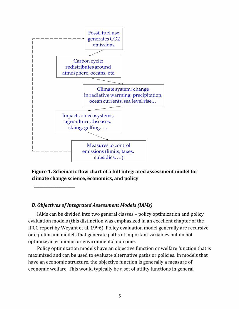
Figure 1 shows a schematic flow chart of the major modules and logical

structure of the DICE and RICE models.

5

Figure 1. Schematic flow chart of a full integrated assessment model for

climate change science, economics, and policy

______________________

B. Objectives of Integrated Assessment Models (IAMs)

IAMs can be divided into two general classes – policy optimization and policy

evaluation models (this distinction was emphasized in an excellent chapter of the

IPCC report by Weyant et al. 1996). Policy evaluation model generally are recursive

or equilibrium models that generate paths of important variables but do not

optimize an economic or environmental outcome.

Policy optimization models have an objective function or welfare function that is

maximized and can be used to evaluate alternative paths or policies. In models that

have an economic structure, the objective function is generally a measure of

economic welfare. This would typically be a set of utility functions in general

2

Fossil fuel usegenerates CO2

emissions

Carbon cycle: redistributes around

atmosphere, oceans, etc.

Climate system: change in radiative warming, precipitation,

ocean currents, sea level rise,…

Impacts on ecosystems,agriculture, diseases,

skiing, golfing, …

Measures to controlemissions (limits, taxes,

subsidies, …)

6

equilibrium models or consumer and producer surplus in partial equilibrium

models.

These two approaches are not as different as might be supposed, as policy

optimization models can be run in a non-policy mode, while policy evaluation

models can compare different policies. However, there are often differences in the

solution algorithms as recursive models are often much simpler to solve

computationally than are optimization models.

The DICE/RICE models are primarily designed as policy optimization models,

although they can be run as simple projection models as well. In both modes, the

approach is to maximize an economic objective function. The objective function

represents the goal implicit in the problem. For the DICE/RICE models, the objective

function refers to the economic well-being (or utility) associated with a path of

consumption.

As will be emphasized below, the use of optimization can be interpreted in two

ways: First, from a positive point of view, optimization is a means of simulating the

behavior of a system of competitive markets; and, second, from a normative point of

view, it is a possible approach to comparing the impact of alternative paths or

policies on economic welfare. The models are available at dicemodel.net.

III. Detailed Equations of the DICE-2013R Model

A. Preferences and the Objective Function

In the DICE and RICE models, the world or individual regions are assumed to

have well-defined preferences, represented by a social welfare function, which

ranks different paths of consumption. The social welfare function is increasing in the

number of people and in the per capita consumption of each generation, with

diminishing marginal utility of consumption.

The importance of a generation’s per capita consumption depends on the size of

the population. The relative importance of different generations is affected by two

central normative parameters, the pure rate of social time preference (“generational

discounting”) and the elasticity of the marginal utility of consumption (the

“consumption elasticity”). These two parameters interact to determine the discount

rate on goods, which is critical for intertemporal economic choices. In the modeling,

we set the preference parameters to be consistent with observed economic

outcomes as reflected by interest rates and rates of return on capital, a choice that

will be central to the results and is further discussed in the section on discounting

below.

7

The DICE model assumes that economic and climate policies should be designed

to optimize the flow of consumption over time. It is important to emphasize that

consumption should be interpreted as “generalized consumption,” which includes

not only traditional market goods and services like food and shelter but also non-

market items such as leisure, health status, and environmental services.

The mathematical representation of this assumption is that policies are chosen

to maximize a social welfare function, W, that is the discounted sum of the

population-weighted utility of per capita consumption. The notation is that c(t) is

per capita consumption, L(t) is population as well as labor inputs, and R(t) is the

discount factor, all of which are discussed as we proceed. Equation (1) is the

mathematical statement of the objective function. This representation is a standard

one in modern theories of optimal economic growth (see Ramsey 1928, Koopmans

1965, Cass 1965).

1

1T max

t

( ) W U[c(t),L(t)]R(t)

There are a number of further assumptions underlying this choice of an

objective function. First, it involves a specific representation of the value or “utility”

of consumption. The DICE/RICE models assume that utility is represented by a

constant elasticity utility function, as shown in equation (2).

(2) 1-U [ c(t),L(t)] = L(t)[ c(t) / (1- )]

This form assumes a constant elasticity of the marginal utility of consumption, α.

(In the limiting case where α = 1, the utility function is logarithmic.) The elasticity

parameter is best thought of as aversion to generational inequality. Put differently,

the elasticity represents the diminishing social valuations of consumption of

different generations. If α is close to zero, then the consumptions of different

generations are close substitutes, with low aversion to inequality; if α is high, then

the consumptions are highly differentiated, and this reflects high inequality

aversion. Often, α will also be used to represent risk aversion, but these are strictly

speaking quite distinct concepts and should not be confused (see Epstein and Zin

1989, 1991). Additionally, the elasticity is distinct from the personal behavioral

characteristics. We calibrate α in conjunction with the pure rate of time preference,

as is discussed below.

Second, this specification assumes that the value of consumption in a period is

proportional to the population. In the RICE model, the presence of multiple agents

8

will lead to major issues of interpretation and computation, but this is not relevant

in the DICE model and will be largely ignored in this manual.

Third, this approach applies a discount on the economic well-being of future

generations, as is defined in Equation (3).

(3) -tR(t) (1+ ρ)

In this specification, R(t) is the discount factor, while the pure rate of social time

preference, ρ , is the discount rate which provides the welfare weights on the

utilities of different generations.

We should add a note of interpretation of the equilibrium in the DICE model. We

have specified the baseline case so that, from a conceptual point of view, it

represents the outcome of market and policy factors as they currently exist. In other

words, the baseline model is an attempt to project from a positive perspective the

levels and growth of major economic and environmental variables as would occur

with current climate-change policies. It does not make any case for the social

desirability of the distribution of incomes over space or time of existing conditions,

any more than a marine biologist makes a moral judgment on the equity of the

eating habits of sharks or guppies.

We can put this point differently in terms of welfare improvements. The

calculations of the potential improvements in world welfare from efficient climate-

change policies examine potential improvements within the context of the existing

distribution of income and investments across space and time. There may be other

improvements – in local pollution policies, in tax or transfer programs, or in

international aid programs – that would improve the human condition, and might

improve it even more than the policies we consider, but these are outside the scope

of this analysis. This point is discussed at length in Nordhaus (2012).

B. Economic Variables

The economic sectors of the DICE model are standard to the economic growth

literature. The main difference from standard analysis is the very long time frame

that is required for climate-change modeling. While most macroeconomic models

run for a few years, or in the development context a few decades, climate-change

projects necessarily must encompass more than a century. The result is that many of

the projections and assumptions are based on very thin evidence.

We begin with the standard neoclassical decisions about capital accumulation

and then consider the geophysical constraints. The DICE/RICE models are simplified

9

relative to many models because they assume a single commodity, which can be

used for consumption, investment, or abatement. Consumption should be viewed

broadly to include not only food and shelter but also non-market environmental

amenities and services.

The output, population, and emissions variables are built up from national data.

They are generally aggregated into major regions (United States, China, EU, India,

and so forth). They are then projected separately. The regional aggregates are used

in the RICE model. For the DICE model, they are simply aggregated together for the

world total.

Each region is endowed with an initial stock of capital and labor and an initial

and region-specific level of technology. Population growth and technological change

are region-specific and exogenous, while capital accumulation is determined by

optimizing the flow of consumption over time for each region. Regional outputs and

capital stocks are aggregated using purchasing power parity (PPP) exchange rates

(although this has been controversial, see IPCC Fourth Assessment, Mitigation 2007

and Nordhaus 2007a).

We next describe the equations for the different economic variables in the DICE-

2013R model. The first set of equations determines the evolution of world output

over time. Population and the labor force are exogenous. These are simplified to be

logistic-type equations of the form   LL t = L t - 1 1+ g t , where

L L Lg t = g t - 1 1+ δ . The initial population in 2010 is given, and the growth rate

declines so that total world population approaches a limit of 10.5 billion in 2100.

The initial growth rate of population, gL(2015), of 13.4% per period (5 years) is set

so that population equals the UN projection for 2050. These numbers have been

revised upward in line with the most recent UN projections and are about 20

percent higher than the 2007 DICE/RICE model estimates. (A fine recent review is

Lee 2011 and other articles in the same issue.)

Output is produced with a Cobb-Douglas production function in capital, labor,

and energy. Energy takes the form of either carbon-based fuels (such as coal) or

non-carbon-based technologies (such as solar or geothermal energy or nuclear

power).

Technological change takes two forms: economy-wide technological change and

carbon-saving technological change. The level of total factor productivity [TFP,

represented by A(t)] is a logistic equation similar to that of population. It takes the

form AA t = A t - 1 1+ g t , where A A Ag t = g t - 1 1+ δ . In this specification,

TFP growth declines over time. In the current specification, A(2010) is set to to

10

calibrate the model to gross world product in 2010; gA(2015) = 7.9 % per five years;

and δA = 0.6% per five years. This specification leads to growth in consumption per

capita of 1.9% per year from 2010 to 2100 and 0.9% per year from 2100 to 2200.

Carbon-saving technological change is modeled as reducing the ratio of CO2

emissions to output (described below). Carbon fuels are limited in supply, with a

total limit of 6000 billion tons of carbon content. In the current version, the carbon

constraint is not binding in the base case. Substitution from carbon to non-carbon

fuels takes place over time as carbon-based fuels become more expensive, either

because of resource exhaustion or because policies are taken to limit carbon

emissions.

The underlying population and output estimates are aggregated up from a

twelve-region model. Outputs are measured in purchasing power parity (PPP)

exchange rates using the IMF estimates (Nordhaus 2007a). Total output for each

region is projected using a partial convergence model, and the outputs are then

aggregated to the world total. The regional and global production functions are

assumed to be constant-returns-to-scale Cobb-Douglas production functions in

capital, labor, and Hicks-neutral technological change. Global output is shown in

Equation (4):

1(4) 1 1Q(t) [ (t)]A(t)K(t) L(t) / [ (t)]

In this specification, Q(t) is output net of damages and abatement, A(t) is total

factor productivity (of the Hicks-neutral variety), and K(t) is capital stock and

services. The additional variables in the production function are (t) and (t) ,

which represent climate damages and abatement costs, shown in Equations (5) and

(6).

(5) 21 AT 1 AT (t) = ψ T (t)+ψ [ T (t) ]

Equation (5) involves the economic damages or impacts of climate change,

which is the thorniest issue in climate-change economics. These estimates are

indispensable for making sensible decisions about the appropriate balance between

costly emissions reductions and climate damages. However, providing reliable

estimates of the damages from climate change over the long run has proven

extremely difficult.

The damage function in (5) has been greatly simplified from earlier DICE/RICE

versions. Earlier versions relied on detailed sectoral estimates from Nordhaus and

11

Boyer (2000). However, further work indicated that those estimates were

increasingly outdated and unreliable.

The 2013 model instead uses a highly simplified damage function that relies on

current estimates of the damage function. More precisely, DICE-2013R uses

estimates of monetized damages from the Tol (2009) survey as the starting point.

However, current studies generally omit several important factors (the economic

value of losses from biodiversity, ocean acidification, and political reactions),

extreme events (sea-level rise, changes in ocean circulation, and accelerated climate

change), impacts that are inherently difficult to model (catastrophic events and very

long term warming), and uncertainty (of virtually all components from economic

growth to damages). I have added an adjustment of 25 percent of the monetized

damages to reflect these non-monetized impacts. While this is consistent with the

estimates from other studies (see Hope 2011, Anthoff and Tol 2010, and FUND

2013), it is recognized that this is largely a judgmental adjustment. The current

version assumes that damages are a quadratic function of temperature change and

does not include sharp thresholds or tipping points, but this is consistent with the

survey by Lenton et al. (2008).

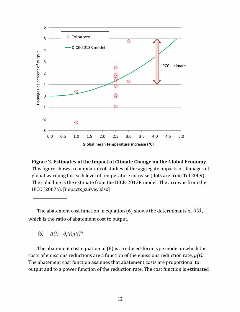
Figure 2 shows the results of the Tol (2009) survey on damages, the IPCC

assessment from the Third and Fourth Assessment Reports, and the assumption in

the DICE-2013R model as a function of global mean temperature increase.

I would note an important warning about the functional form in equation (5)

when using for large temperature increases. The damage function has been

calibrated for damage estimates in the range of 0 to 3 °C. In reality, estimates of

damage functions are virtually non-existent for temperature increases above 3 °C.

Note also that the functional form in (5), which puts the damage ratio in the

denominator, is designed to ensure that damages do not exceed 100% of output, and

this limits the usefulness of this approach for catastrophic climate change. The

damage function needs to be examined carefully or re-specified in cases of higher

warming or catastrophic damages.

12

Figure 2. Estimates of the Impact of Climate Change on the Global Economy

This figure shows a compilation of studies of the aggregate impacts or damages of

global warming for each level of temperature increase (dots are from Tol 2009).

The solid line is the estimate from the DICE-2013R model. The arrow is from the

IPCC (2007a). [impacts_survey.xlsx]

__________________

The abatement cost function in equation (6) shows the determinants of Λ(t) ,

which is the ratio of abatement cost to output.

2θ1(6) Λ(t) = θ (t)μ(t)

The abatement cost equation in (6) is a reduced-form type model in which the

costs of emissions reductions are a function of the emissions reduction rate, μ(t).

The abatement cost function assumes that abatement costs are proportional to

output and to a power function of the reduction rate. The cost function is estimated

-3

-2

-1

0

1

2

3

4

5

6

0.0 0.5 1.0 1.5 2.0 2.5 3.0 3.5 4.0 4.5 5.0

Dam

ages

as

per

cen

t o

f o

utp

ut

Global mean temperature increase (°C)

Tol survey

DICE-2013R model

IPCC estimate

13

to be highly convex, indicating that the marginal cost of reductions rises from zero

more than linearly with the reductions rate.

The DICE-2013R model explicitly includes a backstop technology, which is a

technology that can replace all fossil fuels. The backstop technology could be one

that removes carbon from the atmosphere or an all-purpose environmentally

benign zero-carbon energy technology. It might be solar power, or carbon-eating

trees or windmills, or some as-yet undiscovered source. The backstop price is

assumed to be initially high and to decline over time with carbon-saving

technological change.

In the full regional model, the backstop technology replaces 100 percent of

carbon emissions at a cost of between $230 and $540 per ton of CO2 depending

upon the region in 2005 prices. For the global DICE-2013R model, the 2010 cost of

the backstop technology is $344 per ton CO2 at 100% removal. The cost of the

backstop technology is assumed to decline at 0.5% per year. The backstop

technology is introduced into the model by setting the time path of the parameters

in the abatement-cost equation (6) so that the marginal cost of abatement at a

control rate of 100 percent is equal to the backstop price for a given year.

The next three equations are standard economic accounting equations. Equation

(7) states that output includes consumption plus gross investment. Equation (8)

defines per capita consumption. Equation (9) states that the capital stock dynamics

follows a perpetual inventory method with an exponential depreciation rate.

(7) Q(t) = C(t)+ I(t)

(8) c(t) = C(t) / L(t)

K(9) K(t) = I(t) - δ K(t -1)

CO2 emissions are projected as a function of total output, a time-varying

emissions-output ratio, and the emissions-control rate. The emissions-output ratio

is estimated for individual regions and is then aggregated to the global ratio. The

emissions-control rate is determined by the climate-change policy under

examination. The cost of emissions reductions is parameterized by a log-linear

function, which is calibrated to the EMF-22 report and the models contained in that

(Clarke et al. 2010).

Early versions of the DICE and RICE models used the emissions control rate as

the control variable in the optimization because it is most easily used in linear-

program algorithms. In recent versions, we have also incorporated a carbon tax as a

control variable. This can be accomplished using an Excel SOLVER version with a

14

modified Newton method to find the optimum. It can also be used in the GAMS

version if the carbon price is solved explicitly (which can be done in the current

version). The carbon price is determined by assuming that the price is equal to the

marginal cost of emissions. The marginal cost is easily calculated from the

abatement cost equation in (6) and by substituting the output equations.

The final two equations in the economic module are the emissions equation and

the resource constraint on carbon fuels. Baseline industrial CO2 emissions in

Equation (10) are given by a level of carbon intensity, σ(t), times output. (See the

change in the definition of the baseline below.) Actual emissions are then reduced

by one minus the emissions-reduction rate, [1-μ(t)].

γ 1-γ

Ind(10) E (t) = σ(t)[1- μ(t)]A(t) K(t) L(t)

The carbon intensity is taken to be exogenous and is built up from emissions

estimates of the twelve regions, whereas the emissions-reduction rate is the control

variable in the different experiments. Estimates of baseline carbon intensity are a

logistics-type equation similar to that of total factor productivity. It takes the form

t = t - 1 1+ g t , where σ σ σg t = g t - 1 / 1+ δ . In the current

specification, σ(2010) is set to equal the carbon intensity in 2010, 0.549 tons of CO2

per $1000 of GDP; gσ(2015) = -1.0% per year; and δσ = -0.1% per five years. This

specification leads to rate of change of carbon intensity (with no climate change

policies) of -0.95%per year from 2010 to 2100 and -0.87% per year from 2100 to

2200.

Equation (11) is a limitation on total resources of carbon fuels, given by CCum.

In earlier versions, the carbon constraint was binding, but it is not in the current

version. The model assumes that incremental extraction costs are zero and that

carbon fuels are efficiently allocated over time by the market. We have simplified

the current version by deleting the complicated Hotelling procedure as unnecessary

because the resource constraint was not binding. This can produce problems, as is

noted in the program, if emissions growth is much higher than the baseline. The

limit in the DICE-2013R model has not changed from earlier versions and is 6000

tons of carbon content.

1

(11) T max

Indt

CCum E (t)

Cumulative carbon emissions from 2010 to 2100 in the baseline DICE-2013R model

are projected to be 1870 GtC, and for the entire period 4800 GtC. Estimates for 2100

15

are slightly higher than the models surveyed in the IPCC Fifth Assessment Report,

Science (2013), Figure 6.25.

C. Geophysical sectors

The DICE-2013R model includes several geophysical relationships that link the

economy with the different forces affecting climate change. These relationships

include the carbon cycle, a radiative forcing equation, climate-change equations, and

a climate-damage relationship. A key feature of IAMs is that the modules operate in

an integrated fashion rather than taking variables as exogenous inputs from other

models or assumptions.

The structure of the geophysical sectors is largely unchanged from the last

versions, although the parameters and initial conditions are updated. Equations

(12) to (18) below link economic activity and greenhouse-gas emissions to the

carbon cycle, radiative forcings, and climate change. These relationships were

developed for early versions of the DICE model and have remained relatively stable

over recent revisions. They need to simplify what are inherently complex dynamics

into a small number of equations that can be used in an integrated economic-

geophysical model. As with the economics, the modeling philosophy for the

geophysical relationships has been to use parsimonious specifications so that the

theoretical model is transparent and so that the optimization model is empirically

and computationally tractable.

In the DICE-2013R model, the only GHG that is subject to controls is industrial

CO2. This reflects the fact that CO2 is the major contributor to global warming and

that other GHGs are likely to be controlled in different ways (the case of the

chlorofluorocarbons through the Montreal Protocol being a useful example). Other

GHGs are included as exogenous trends in radiative forcing; these include primarily

CO2 emissions from land-use changes, other well-mixed GHGs, and aerosols.

Recall that equation (10) generated industrial emissions of CO2. Equation (12)

then generates total CO2 emissions as the sum of industrial and land-use emissions.

CO2 arising from land-use changes are exogenous and are projected based on

studies by other modeling groups and results from the Fifth Assessment of the IPCC.

Current estimates are that land-use changes contribute about 3 GtCO2 per year

(IPCC Fifth Assessment, Science, 2013, Chapter 6).

(12) Ind LandE(t) = E (t) + E (t)

16

The carbon cycle is based upon a three-reservoir model calibrated to existing

carbon-cycle models and historical data. We assume that there are three reservoirs

for carbon. The variables MAT(t), MUP(t), and MLO(t) represent carbon in the

atmosphere, carbon in a quickly mixing reservoir in the upper oceans and the

biosphere, and carbon in the deep oceans. Carbon flows in both directions between

adjacent reservoirs. The mixing between the deep oceans and other reservoirs is

extremely slow. The deep oceans provide a large sink for carbon in the long run.

Each of the three reservoirs is assumed to be well-mixed in the short run. Equations

(13) through (15) represent the equations of the carbon cycle.

11 21(13) 1 1AT AT UPM (t) E(t) M (t - ) M (t - )

12 22 32(14) 1 1 1UP AT UP LOM (t) M (t - ) M (t - ) M (t - )

23 33(15) 1 1LO UP LOM (t) M (t - ) M (t - )

The parameters ij represent the flow parameters between reservoirs. Note that

emissions flow into the atmosphere.

The carbon cycle is limited because it cannot represent the complex interactions

of ocean chemistry and carbon absorption. We have adjusted the carbon flow

parameters to reflect carbon-cycle modeling for the 21st century, which show lower

ocean absorption than for earlier periods. This implies that the model overpredicts

atmospheric absorption during historical periods. The impact of a 100 GtC pulse is

that 35% remains in the atmosphere after 100 years. It is useful to compare this

with the results from the Fifth Assessment Report of the IPCC. The DICE model

atmospheric concentrations 100 years after a pulse are lower than the average of

models, which is around 40% IPCC (IPCC Fifth Assessment, Science, 2013, Box 6.1,

Fig. 1, p. 6-122).

The next step concerns the relationship between the accumulation of GHGs and

climate change. The climate equations are a simplified representation that includes

an equation for radiative forcing and two equations for the climate system. The

radiative forcing equation calculates the impact of the accumulation of GHGs on the

radiation balance of the globe. The climate equations calculate the mean surface

temperature of the globe and the average temperature of the deep oceans for each

time-step.

Accumulations of GHGs lead to warming at the earth’s surface through increases

in radiative forcing. The relationship between GHG accumulations and increased

17

radiative forcing is derived from empirical measurements and climate models, as

shown in Equation (16).

2(16) AT AT EXF(t) {log [M (t) / M (1750)]} F (t)

F(t) is the change in total radiative forcings of greenhouse gases since 1750 from

anthropogenic sources such as CO2. FEX(t) is exogenous forcings, and the first term is

the forcings due to CO2.

The equation uses estimated carbon in different reservoirs in the year 1750 as

the pre-industrial equilibrium. The major part of future warming is projected to

come from to CO2, while the balance is exogenous forcing from other long-lived

greenhouse gases, aerosols, ozone, albedo changes, and other factors. The DICE

model treats other greenhouse gases and forcing components as exogenous either

because these are relatively small, or their control is exogenous (as the case of

CFCs), or because they are poorly understood (as with cloud albedo effects).

Estimates of future impacts of aerosols have proven challenging, and the current

model uses estimates from the scenarios prepared for the Fifth Assessment of the

IPCC. The estimates in DICE-2013R are drawn from the guidance for the

“Representative Concentration Pathways" (RCPs, see

http://tntcat.iiasa.ac.at:8787/RcpDb/ dsd?Action=htmlpage&page=compare). The

high path has exceptionally high and unreasonable estimates of methane forcings.

The estimates here use the RCP 6.0 W/ m2 representative scenario, which is more

consistent with the other scenarios and with historical trends. These estimate non-

CO2 forcings of 0.25 W/m2 in 2010 and 0.7 W/m2 in 2100. Non-CO2 forcings are

small relative to estimated CO2 forcings, with 6.5 W/m2 of forcings from CO2 in 2100

in the DICE baseline projection.

Higher radiative forcing warms the atmospheric layer, which then warms the

upper ocean, gradually warming the deep ocean. The lags in the system are

primarily due to the diffusive inertia of the different layers.

1 2 3(17) 1 1 1 1AT AT AT AT LOT (t) T (t ) {F(t) - T (t ) - [T (t ) -T (t )]}

4(18) 1 1 1LO LO AT LOT (t) T (t ) {T (t ) -T (t )]}

TAT(t) and TLO(t) represent respectively the mean surface temperature and the

temperature of the deep oceans. Note that the equilibrium temperature sensitivity is

given by 2 =ATT F(t) / .

18

A critical parameter is the equilibrium climate sensitivity (°C per equilibrium

CO2 doubling). The method for determining that parameter has been changed in the

most recent model. The precise procedure for the new estimates and the calibration

is the following: Earlier estimates of the climate sensitivity in the DICE model relied

exclusively on estimates from GCMs. However, there is increasing evidence from

other sources, such as the historical record. In the DICE 2013 model, we used a

synthesis of the different sources, and took a weighted average of the estimates. The

revised estimate is a climate sensitivity of 2.9 °C for an equilibrium CO2 doubling.

This revision is based largely on data from a systematic survey of recent

evidence in Knutti and Hegerl (2008). The procedure used for the estimate is to take

a weighted average of the estimates of temperature sensitivity from different

estimation techniques. The current version combines estimates from instrumental

records, the current mean climate state, GCMs, the last millennium, volcanic

eruptions, the last glacial maximum (data and models), long-term proxy records,

and expert assessments. The weights are from the author, with most of the weights

on the model results and the instrumental and historical record. Because the

historical record provides a lower estimate, this combined procedure lowers the

equilibrium sensitivity slightly (to 2.9 °C for an equilibrium CO2 doubling).

Note that this reduction is paralleled by a reduction of the lower bound estimate

of the TSC in the IPCC’s Fifth Assessment Report from 2 °C to 1.5 °C. Additionally, a

visual inspection of the summary of different probabilistic assessments in the Fifth

Assessment Report indicates that the range of estimates using different techniques

is in the range of 1.8 °C to 3.0 °C. An interesting feature is that the climate models

are at the high end of the different techniques, with a mean of the ensemble of 3.2 °C

in the Fifth Report (see IPCC Fifth Assessment, Science, 2013, Chapter 9, especially

Table 9-2).

A further change is to adjust the parameters of the model to match the transient

temperature sensitivity for models with an equilibrium sensitivity of 2.9 °C. The

relationship between equilibrium and transient climate sensitivity uses the

estimates of those two parameters from the IPCC Fifth Assessment Report, which

provided both transient and equilibrium temperature sensitivities for several

models. We used regression analyses to estimate the transient sensitivity at 2.9 °C

equilibrium. The parameterized transient sensitivity from the regressions is set at

1.70 °C. This is done by changing the diffusion parameter 1 (similar to the standard

calibrating parameter in simple energy-balance models of the vertical diffusivity) to

0.98.

19

This completes the description of the DICE model. We now turn to describe the

difference between the DICE and RICE models.

D. The RICE-2010 Model

The RICE model (Regional Integrated model of Climate and the Economy) is a

regionalized version of the DICE model. It has the same basic economic and

geophysical structure, but contains a regional elaboration. The last full version is

described in Nordhaus (2010), with detailed in the Supplemental Information to

Nordhaus (2010).

The general structure of the RICE model is similar to the DICE model with

disaggregation into regions. However, the specification of preferences is different

because it must encompass multiple agents (regions). The general preference

function is a Bergson-Samuelson social welfare function over regions of the form

1

( , , ),N

W U UW where I

U is the preference function of the Ith region. The

model is specified using the Negishi approach in which regions are aggregated using

time- and region-specific weights subject to budget constraints, yielding

1 1

19T max N

I I I II , t

t I

( ) W U [c (t),L (t)]R (t)

In this specification, the I , t are the “Negishi weights” on each region and each time

period. Each region has individual consumption and population. In principle, they

may have different rates of time preference, although in practice the RICE model

assumes that they are all equal. The Negishi algorithm in the RICE model sets each

of the weights so that the marginal utility of consumption is equal in each region and

each period, which ensures that the requirement for maximization as market

simulation principle holds. We elaborate below on the Negishi approach, which is

widely used in IAMs for climate change, in the section on “Computational and

algorithmic aspects.“

The RICE-2010 model divides the world into 12 regions. These are US, EU,

Japan, Russia, Eurasia (Eastern Europe and several former Soviet Republics), China,

India, Middle East, Sub-Saharan Africa, Latin America, Other high income countries,

and Other developing countries. Note that some of the regions are large countries

such as the United States or China; others are large multi-country regions such as

the European Union or Latin America.

20

Each region is assumed to produce a single commodity, which can be used for

consumption, investment, or emissions reductions. Each region is endowed with an

initial stock of capital and labor and with an initial and region-specific level of

technology. Population data are from the United Nations, updated with more recent

estimates through 2009, with projections using the United Nations’ estimates to

2300. Output is measured as standard gross domestic product (GDP) in constant

prices, and the GDPs of different countries are converted into constant U.S.

international prices using purchasing-power-parity exchange rates. Output data

through 2009 are from the World Bank and the International Monetary Fund (IMF),

with projections to 2014 from the IMF. CO2 emissions data are from the U.S. Energy

Information Administration and Carbon Dioxide Information Analysis Center and

are available in preliminary form through 2008.

The population, technology, and production structure is the same as in the DICE

model. However, each region has its own levels and trends for each variable. The

major long-run variable is region-specific technological change, which is projected

for a frontier region (the United States), and other countries are assumed to

converge partially to the frontier.

The geophysical equations are basically the same as the DICE model as of 2010,

but they differ slightly from the current version. The major difference is that there

are region-specific land-use CO2 emissions, but these are exogenous and have little

effect on the outcomes.

The objective function used in the RICE model differs from that in the DICE

model. Each region is assumed to have a social welfare function, and each region

optimizes its consumption, GHG policies, and investment over time. The parameters

for each region are calibrated to ensure that the real interest rate in the model is

close to the average real interest rate and the average real return on capital in real-

world markets in the specific region. We interpret the output and calibration of

optimization models as “markets as maximization algorithms” (see Nordhaus 2012

for a discussion). We do not view the solution as one in which a world central

planner is allocating resources in an optimal fashion. Rather, output and

consumption is determined according to the initial endowments of technology.

“Dollar votes” in the RICE model may not correspond to any ethical norms but

instead reflects the laws of supply and demand. To put this in terms of standard

welfare economics, the outcome is optimal in the sense of both efficient and fair if

the initial endowments are ethically appropriate, but without that assumption we

can only label the outcome as Pareto efficient.

21

E. Interpretation of Positive and Normative Models (*)

One of the issues that pervades the use of IAMs is whether they should be

interpreted as normative or positive.2 In other words, should they be seen as the

recommendations of a central planner, a world environmental agency, or a

disinterested observer incorporating a social welfare function? Or are they meant to

be a description of how economies and real-world decision makers (consumers,

firms, and governments) actually behave? This issue also arises in the analysis of the

discount rate.

For most simulation models, such as general circulation climate models, the

interpretation is clearly that these are meant to be descriptive. The interpretation of

optimization models is more complex, however. In some cases, the purpose is

clearly normative. For example, the Stern Review represented an attempt to provide

normative guidance on how to cope with the dangers raised by climate change. In

other cases, such as baseline projections, these are clearly meant to be descriptive.

The ambiguity arises particularly because many models use optimization as a

technique for calibrating market outcomes in a positive approach. This is the

interpretation of “market mechanisms as maximization or minimization devices.”

The question was addressed in one of the earliest energy-model comparisons,

chaired by Tjalling Koopmans, “The use of optimization in these models should be

seen as a means of simulating, as a first approximation, the behavior of a system of

interacting competitive markets.” (MRG 1978, p. 5, emphasis added.)

This point was elaborated at length in the integrated assessment study of

copper by Gordon, Koopmans, Nordhaus, and Skinner (1987, with minor edits to

simplify and emphasis added):

We can apply this result to our problem of exhaustible resources as

follows: if each firm is faced with the same market prices for its inputs and

outputs, and if each firm chooses its activities so as to maximize the firm's

discounted profits, then the outcome will be economically efficient. In more

precise language, such an equilibrium will be economically efficient in the

sense that (1) each firm will provide its share of the market at minimum

discounted cost; and (2) the requirements of the market will be met by

producers in a manner that satisfies total demand at minimum discounted

total cost to society.

Examining these two conditions, we see that our competitive

equilibrium has indeed solved a minimization problem of sorts – it has found

2 This section draws heavily on Nordhaus (2012).

22

a way of providing the appropriate array of services at lowest possible costs.

But this minimization is exactly the objective of a linear-programming

problem as well. Consequently, we can mimic the outcome of the economic

equilibrium by solving the LP problem that minimizes the same set of cost

functions subject to the same set of technical constraints. Put differently,

given the appropriate quantities of resources available and the proper

demand requirements, by solving a cost-minimizing LP problem we can

determine the equilibrium market prices and quantities for all future periods.

We call this lucky analytical coincidence the correspondence principle:

determining the prices and quantities in a general economic equilibrium and

solving the embedded cost-minimization problem by linear programming are

mathematically equivalent.

This discussion implies that we can interpret optimization models as a device

for estimating the equilibrium of a market economy. As such, it does not necessarily

have a normative interpretation. Rather, the maximization is an algorithm for

finding the outcome of efficient competitive markets.

F. Consistency with the IPCC Fifth Assessment Report (*)

The DICE-2013R was developed over the 2012-13 period and launched shortly

after the release of the Working Group I report of the IPCC, or “AR5” (IPCC, Fifth

Assessment Report, Science, 2013). Most of the results of AR5 were available before

the release, and as a result the geophysical modules were largely consistent with the

final report.

Among the major findings of AR5 that relate to the DICE-2013R model, here are

the major ones:

The range of estimates of the climate sensitivity was increased from 2.0 –

4.5 to 1.5 – 4.5 °C, which is assessed to be the likely range of equilibrium

climate sensitivity. (The IPCC uses the term “likely” to represent 66–100%

probability.) There were no major changes in the average climate sensitivity

of the ensemble of models.

AR5 contained an extended discussion of alternative estimates of the

climate sensitivity using different approaches. The summary statistics of the

alternatives was between 1.8 °C and 3.0 °C. The new approach to climate

sensitivity is consistent with the trend toward looking at a broader array of

sources for that parameter. (p. TS-113)

23

The results of the carbon cycle models were largely unchanged from the

Fourth Report. See the discussion of the carbon cycle above. (AR5, Chapter

6)

AR5 used a completely different approach to scenario modeling. It relied on

““Representative Concentration Pathways" (RCPs) as a replacement for the

SRES approach to scenarios. As the report states, “These RCPs represent a

larger set of mitigation scenarios and were selected to have different targets

in terms of radiative forcing at 2100 (about 2.6, 4.5, 6.0 and 8.5 W m–2; see

Figure TS.15). The scenarios should be considered plausible and illustrative,

and do not have probabilities attached to them. “ (p. TS-44) As noted below,

this opens up a large gap between economic analysis and global-warming

science.

The DICE-2013R baseline radiative forcings is close to the RCP 8.5 forcing

estimates through 2100, then midway between the RCP 8.5 and RCP 6.0

after 2150. The DICE temperature projection for the baseline scenario is

very close to the model ensemble for the RCP 8.5 through 2200. This

suggests that the DICE-2015R has a short-run temperature sensitivity that

is slightly higher than the AR5 model ensemble. (Figures 12.4, 12.5)

Emissions in the baseline are close to those of the RCP 8.5 scenario. Total

CO2 emissions in the DICE baseline total 103 GtCO2 compared to 106 GtCO2

in RCP 8.5. Cumulative CO2 emissions in the DICE baseline are 1889 GtC

compared to 1750- 1900 GtC in the models used for RCP 8.5. (p. I-60, I-61)

I close with a final word on the limitations of the RCPs. They have the strong

advantage of providing a coherent set of inputs for the calculations of climate and

ecological models. However, the RCP are only weakly linked back to the economic

drivers of emissions. The models that produce the concentrations and forcings are

based on economic and energy models. However, there is no attempt to harmonize

the output, population, emissions, and other driving variables across different

scenarios. Putting this differently, the IPCC RCPs have very little value in integrating

the economic policies and variables with the geophysical calculations and

projections.

24

IV. Results from the DICE-2013R Model (*)

A. Scenarios

Integrated assessment models have a wide variety of applications. Among the

most important applications are the following:

Making consistent projections, i.e., ones that have consistent inputs and

outputs of the different components of the system (for example, so that the

world output projections are consistent with the emissions projections).

Calculating the impacts of alternative assumptions on important variables

such as output, emissions, temperature change, and impacts.

Tracing through the effects of alternative policies on all variables in a

consistent manner, as well as estimating the costs and benefits of

alternative strategies.

Estimating the uncertainties associated with alternative variables and

strategies.

Calculating the effects of reducing uncertainties about key parameters or

variables, as well as estimating the value of research and new technologies.

With these objectives in mind, this section presents illustrative results for

different scenarios using the DICE-2013R model. We present the results of five

scenarios.

Baseline: Current policies as of 2010 are extended indefinitely. The

conceptual definition of the baseline scenario has changed from earlier

versions. In earlier runs, “baseline” meant “no policies.” In the current version,

base is existing policies as of 2010. This approach is standard for forecasting,

say of government budgets, and is more appropriate for a world of evolving

climate policies. Estimates from Nordhaus (2010) indicate that 2010 policies

were the equivalent of $1 per ton of CO2 global emissions reductions. Note that

is requires calculating baseline emissions intensities as reflecting this level of

emissions reductions.

Optimal: Climate-change policies maximize economic welfare, with full

participation by all nations starting in 2015 and without climatic constraints.

The “optimal” scenario assumes the most efficient climate-change policies; in

this context, efficiency involves a balancing of the present value of the costs of

abatement and the present value of the benefits of reduced climate damages.

Although unrealistic, this scenario provides an efficiency benchmark against

which other policies can be measured.

25

Temperature-limited: The optimal policies are undertaken subject to a further

constraint that global temperature does not exceed 2 °C above the 1900

average. The “temperature-limited” scenario is a variant of the optimal scenario

that builds in a precautionary constraint that a specific temperature increase is

not exceeded. This scenario is also consistent with the goals adopted under the

“Copenhagen Accord,” although countries have not adopted national targets

that would reach this limit.

Low discounting according to Stern Review. The Stern Review advocated using

very low discount rates for climate-change policy. This was implemented using

a time discount rate of 0.1 percent per year and a consumption elasticity of 1.

This leads to low real interest rates and generally to higher carbon prices and

emissions control rates.

Low time preference with calibrated interest rates. Because the Stern Review

run leads to real interest rates that are below the assumed level, we adjust the

parameters of the preference function to match the calibrated real interest

rates. This run draws on the Ramsey equation; it keeps the near-zero time

discount rate and calibrates the consumption elasticity to match observable

variables on average through 2040. The calibration keeps the rate of time

preference at 0.1 percent per year but raises the consumption elasticity to 2.1.

Copenhagen Accord. In this scenario, high-income countries are assumed to

implement deep emissions reductions over the next four decades, with

developing countries following gradually. It is assumed that implementation is

through system of national emission caps with full emissions trading within

and among countries (although a harmonized carbon tax would lead to the

same results). We note that most countries are not on target to achieving these

goals.

B. Major Results (*)

We present a limited set of results for the different scenarios. The full results are

available in a spreadsheet on request from the author.

Table 1 and Figures 3 - 5 show the major economic variables in the different

scenarios. These show rapid projected economic growth. The real interest rate is a

critical variable for determining climate policy.

26

Figure 3. Global output 2010-2100 under alternative policies, DICE-2013R model [Sources for Figures 3 – 10: Graphicsv5_manual_051713.xlsm]

0

100

200

300

400

500

600

2010 2020 2030 2040 2050 2060 2070 2080 2090 2100

Ou

tpu

t (N

et

of

Da

ma

ges

an

d A

ba

tem

en

t, t

rill

ion

US

$)

Year

Global output

Base Opt

Lim2t Stern

SternCalib Copen

27

Figure 4. Per capita consumption 2010-2100 under alternative policies, DICE-

2013R model

Figure 5. Real interest rate in alternative runs Note that the real interest rates are similar except for the Stern run, in which case real interest rates are much lower. __________________

0

5

10

15

20

25

30

35

40

45

50

2000 2010 2020 2030 2040 2050 2060 2070 2080 2090 2100

Pe

r ca

pit

a co

nsu

mp

tio

n (1

00

0s

of 2

00

5 U

S$)

Per Capita ConsumptionBase

Optimal

Lim2t

Stern

SternCalib

Copen

0

0.01

0.02

0.03

0.04

0.05

0.06

2010 2020 2030 2040 2050 2060 2070 2080 2090 2100

Inte

rest

Rat

e (R

eal R

ate

of

Ret

urn

)

Year

Real interest Rate

Base Opt

Lim2t Stern

SternCalib Copen

28

Table 1. Major economic variables in different scenarios

[Source: Excel_Handbook_TandG_110711a_092713.xlsx, tab 1-3]

______________________

Table 2 and Figures 6 - 8 show the major environment variables: industrial CO2

emissions, atmospheric CO2 concentrations, and global mean temperature increase.

The model projects substantial warming over the next century and beyond if no

controls are taken. Baseline temperature is projected to be around 3.8°C above 1900

levels by 2100, and continuing to rise after that. Atmospheric concentrations of CO2

are estimated to be 858 ppm in 2100. Total radiative forcings in 2100 for the

baseline case are 6.9 W/m2, which is about 1 W/m2 below the high case in the IPCC

runs for the Fifth Assessment Report.

Gross World Output (trillions

2005 US$) 2010 2020 2030 2050 2100 2150 2200

Base 63.58 89.59 121.47 203.19 511.56 951.42 1,487.13

Optimal 63.58 89.66 121.61 203.68 516.42 974.47 1,547.66

Limit T < 2 ⁰C 63.58 89.43 121.15 203.14 515.76 981.90 1,555.38

Stern Discounting 63.58 95.87 132.24 222.75 565.11 1,070.41 1,689.24

Stern Recalibrated 63.58 89.39 121.36 204.46 526.81 1,007.44 1,612.62

Copenhagen 63.58 89.65 121.61 203.57 515.25 972.67 1,538.18

Per Capita Consumption

(1000 2005 US$) 2010 2020 2030 2050 2100 2150 2200

Base 6.886 8.768 11.011 16.600 36.819 64.123 95.981

Optimal 6.878 8.756 10.992 16.567 37.063 67.609 108.390

Limit T < 2 ⁰C 6.897 8.728 10.891 16.112 37.292 69.588 110.419

Stern Discounting 6.103 8.432 10.812 16.361 37.740 70.284 111.996

Stern Recalibrated 6.911 8.743 10.950 16.489 36.984 68.445 109.817

Copenhagen 6.881 8.755 10.974 16.504 37.053 67.951 106.734

Real Interest Rate (% per

year) 2010 2020 2030 2050 2100 2150 2200

Base 5.16% 4.97% 4.74% 4.29% 3.42% 2.86% 2.52%

Optimal 5.16% 4.96% 4.73% 4.30% 3.49% 3.02% 2.71%

Limit T < 2 ⁰C 5.07% 4.87% 4.62% 4.18% 3.65% 3.02% 2.68%

Stern Discounting 3.73% 2.76% 2.37% 2.01% 1.56% 1.14% 0.91%

Stern Recalibrated 5.21% 5.01% 4.73% 4.12% 3.02% 2.32% 1.82%

Copenhagen 5.16% 4.94% 4.70% 4.28% 3.54% 3.03% 2.62%

29

Figure 6. Projected emissions of CO2 under alternative policies, DICE-2013R

model

Note that other GHGs are taken to be exogenous in the projections.

0

20

40

60

80

100

120

2010 2020 2030 2040 2050 2060 2070 2080 2090 2100

Ind

ust

ria

l em

issi

on

s (G

TC

O2

pe

r yea

r)

Year

Industrial CO2 emissions

Base Opt Lim2t

Stern SternCalib Copen

30

Figure 7. Atmospheric concentrations of CO2 under alternative policies, DICE-

2013R model

Projected atmospheric concentrations of CO2 associated with different policies. The

concentrations include emissions from land-use changes. Policies are explained in

text.

0

100

200

300

400

500

600

700

800

900

1000

2010 2020 2030 2040 2050 2060 2070 2080 2090 2100

Atm

osp

he

ric

con

cen

tra

tio

n o

f ca

rbo

n (p

pm

)

Year

CO2 Concentration

Base Opt Lim2t

Stern SternCalib Copen

31

Figure 8. Global temperature increase (°C from 1900) under alternative

policies, DICE-2013R model

Projected global mean temperature paths associated with different policies.

0

1

2

3

4

5

6

7

2000 2020 2040 2060 2080 2100 2120 2140 2160 2180 2200

Atm

osp

he

ric

Tem

pe

ratu

re (d

eg

C a

bo

ve p

rein

du

stri

al)

Year

Global temperature change

Base Opt

Lim2t Stern

SternCalib Copen

32

Table 2. Major geophysical variables in different scenarios

__________

Perhaps the most important outputs of integrated economic models of climate

change are the near-term “carbon prices.” This is a concept that measures the

market price of emissions of GHGs. In a market environment, such as a cap-and-

trade regime, the carbon prices would be the trading price of carbon emission

permits. In a carbon-tax regime, these would be the harmonized carbon tax among

participating regions. If the policy is optimized, then the carbon price is also the

social cost of carbon.

Table 3 and Figures 9 - 10 show policies in the different scenarios. The optimal

carbon price in 2015 is estimated to be $18 per ton of CO2, rising to $52 per ton in

2050 and $143 per ton in 2100. The average increase in the real price is 3.1% from

2015 to 2050 and 2.1% per year from 2050 to 2100. The emissions control rate in

the optimal case starts at 21%, rises to around 39% in 2050, and reaches 79% in

2100. Industrial emissions in the optimal case peak around 2050. I emphasize that

these are global figures, not just those for rich countries.

Industrial CO2 Emissions

(GtCO2/yr) 2010 2020 2030 2050 2100 2150 2200

Base 33.6 42.5 51.9 70.2 102.5 103.0 66.6

Optimal 33.6 34.8 40.0 46.1 25.1 0.0 -30.0

Limit T < 2 ⁰C 33.6 27.1 26.4 10.2 2.7 0.0 -26.8

Stern Discounting 33.6 22.5 22.7 16.1 0.0 0.0 -32.7

Stern Recalibrated 33.6 33.8 38.2 41.6 5.9 0.0 -31.3

Copenhagen 34.6 39.6 43.5 43.5 24.6 14.4 14.9

CO2 concentrations (ppm) 2010 2020 2030 2050 2100 2150 2200

Base 390 425 464 560 858 1,134 1,270

Optimal 390 421 451 513 610 535 372

Limit T < 2 ⁰C 390 417 436 456 402 395 276

Stern Discounting 390 414 428 447 408 388 243

Stern Recalibrated 390 420 449 506 556 482 328

Copenhagen 390 425 459 524 585 574 584

Temperature Increase (⁰C

from 1900) 2010 2020 2030 2050 2100 2150 2200

Base 0.80 1.06 1.35 2.01 3.85 5.36 6.26

Optimal 0.80 1.05 1.32 1.88 3.09 3.30 2.48

Limit T < 2 ⁰C 0.80 1.05 1.29 1.72 2.00 1.99 1.32

Stern Discounting 0.80 1.05 1.27 1.67 2.04 1.96 1.00

Stern Recalibrated 0.83 1.08 1.34 1.87 2.91 2.90 2.04

Copenhagen 0.80 1.06 1.34 1.93 3.02 3.37 3.47

33

Figure 9. Emissions control rates, alternative scenarios, DICE-2013R model

Figure 10. Globally averaged carbon prices, alternative scenarios, DICE-

2013R model

0%

20%

40%

60%

80%

100%

120%

2000 2010 2020 2030 2040 2050 2060 2070 2080 2090 2100

Emis

sio

ns

con

tro

l rat

e (%

of

bas

elin

e)

Emissions Control Rate

Base

Optimal

Lim2t

Stern

SternCalib

Copen

0

50

100

150

200

250

300

2000 2010 2020 2030 2040 2050 2060 2070 2080 2090 2100

Pri

ce o

f ca

rbo

n e

mis

sio

ns

($ p

er

ton

of C

O2

)

Carbon PriceStern

Lim2t

Optimal

SternCalib

Copen

Base

34

Table 3. Major climate-policy variables in different scenarios

_____________________

The requirement for achieving the 2 °C target is ambitious. The global emissions

control rate would be 50% by 2030, and industrial emissions would need to reach

zero by 2060.

Table 4 shows the large stakes involved in climate-change policies as measured

by aggregate costs and benefits. Using the model discount rates, the optimal

scenario raises the present value of world income by $21 trillion, or 0.83% of

discounted income. This is equivalent to an annuity of $904 billion per year at a 4%

annual discount rate. Imposing the 2 °C temperature constraint has a significant

economic penalty, reducing the net benefit by almost half, because of the difficulty of

attaining that target with so much inertia in the climate system. The Copenhagen

Accord with phased-in participation of developing countries has substantial net

benefits, but lack of participation in the “rich only” case reduces the benefits below

the optimal level.

Emissions Control Rate (%) 2010 2020 2030 2050 2100 2150 2200

Base 4% 4% 5% 7% 14% 27% 54%

Optimal 4% 22% 27% 39% 79% 100% 120%

Limit T < 2 ⁰C 4% 39% 52% 87% 98% 100% 118%

Stern Discounting 4% 53% 62% 80% 100% 100% 120%

Stern Recalibrated 4% 24% 30% 45% 95% 100% 120%

Copenhagen 1% 11% 21% 42% 79% 90% 90%

Carbon Price (2005$ per ton

CO2) 2010 2020 2030 2050 2100 2150 2200

Base 1.0 1.2 1.5 2.2 5.9 16.0 43.1

Optimal 1.0 21.2 29.3 51.5 142.8 169.3 182.5

Limit T < 2 ⁰C 1.0 60.1 94.4 216.4 209.4 169.3 176.5

Stern Discounting 1.0 103.7 131.3 190.0 218.1 169.3 182.5

Stern Recalibrated 1.0 25.0 35.9 66.9 199.4 169.3 182.5

Copenhagen 1.0 35.8 85.4 81.9 144.0 140.1 108.7

35

Table 4. Present value of global consumption, different policies, DICE-2013R

model (US international dollars, 2005 prices) [source: Tables_092513.xlsx]

The estimates are the present value of global consumption equivalent for the

entire period. This is equivalent to the present value of utility in consumption

units. The difference in numerical column 3 shows the difference between the

control run and the baseline run. The last column is the constant consumption

annuity that would be generated by different policies.

________________

There are many conclusions that can be drawn from the present modeling

effort. One important result is that, even if countries meet their ambitious objectives

under the Copenhagen Accord, global temperatures are unlikely to keep within the 2

°C objective. This conclusion is reinforced if developing countries delay their full

participation beyond the 2030-2050 timeframe.

V. The Recommendation for a Cumulative Emissions Limit (*)

Scientists in the Fifth Assessment Report suggested a new approach to

climate change targets. They noted that a limit of 2 °C would imply that cumulative

emissions should be limited to 1 trillion (1000 billion) tons of carbon. Since

cumulative emissions to 2010 are, by their calculation, 531 billion, this would allow

469 billion tons of carbon of additional emissions in the future.

Level LevelDifference

from base

Difference

from base

Difference from

base

Difference from

base

Present value of

utility

Present value of

consumption

Present value

of utility

Present value

of

consumption

Difference from

base

Annuity (at 4%

per year)

Trillions of

2005$

Trillions of

2005$

Trillions of

2005$ % of Base

Billions of $ per

year

Base 2685.0 2685.0 0.00 0.00 0.00% 0

Optimal 2706.1 2707.6 21.05 22.60 0.83% 904

Limit T < 2 ⁰C 2686.7 2689.7 1.71 4.63 0.17% 185

Stern Discounting na 2658.0 na -27.00 -1.02% -1,080

Stern Recalibrated na 2706.3 na 21.28 0.79% 851

Copenhagen 2700.1 2701.3 15.03 16.27 0.60% 651

Policy Scenario

36

This proposal is easily implemented in the DICE-2013R model. It involves

putting constrains on future emissions by the recommended amount. The result is

temperature and emissions paths that are slightly higher than the 2 °C limit path,

but with those variables lower than in the optimal path. The path is significantly less

efficient than the optimal plan because it targets an intermediate variable

(cumulative emissions) rather than an ultimate variable (economic welfare). There

are also serious issues involved in negotiating cumulative emissions limits, similar

to those of annual emissions limits. However, this is another useful idea to consider

among alternative architectures. (For a discussion of alternative architectures and

the limitations of quantitative targets, see Nordhaus 2013.)

VI. Revisions from earlier vintages (*)

A. Data and structural revisions (*)

There are several large and small changes in the DICE-2013R model compared

to earlier versions. The prior complete documented version of the DICE model is

Nordhaus (2008), while the last complete version of the regional (RICE) model is in

Nordhaus (2010).

The first revision is that the time step has been changed to five years. This

change is taken because improvements in computational capacities allow the model

to be easily solved with a finer time resolution. The change in the time step also

allows removing several ad hoc procedures designed to calibrate actual dynamic

processes.

A second change is the projection of future output growth. Earlier versions of

the DICE and other IAMs tended to have a stagnationist bias, with the growth rate of

total factor productivity declining rapidly in the coming decades. The current

version assumes continued rapid total factor productivity growth over the next

century, particularly for developing countries.

A third revision incorporates a less rapid decline in the CO2-output ratio in

several regions and for the world, which reflects the last decade’s observations.

Earlier trends (through 2004) showed rapid global decarbonization, at a rate

between 1½ and 2 percent per year. Data through 2010 indicate that

decarbonization has been closer to 1 percent per year. The new version assumes

that, conditional on output growth, uncontrolled CO2 emissions will grow at ½

percent per year faster than earlier model assumptions.

A fourth assumption involves the damage function. This change was discussed

above and will not be repeated here.

37

A fifth revision recalibrates the carbon-cycle and climate models to recent earth

system models. The equilibrium and transient temperature impacts of CO2

accumulation have been revised to include a wider range of estimates. Earlier

versions relied entirely on the estimates from general circulation models (for

example, the ensemble of models used in the IPCC Fourth Assessment Report IPCC

Fourth Assessment, Science 2007). The present version uses estimates from sources

such as the instrumental record and estimates based on the paleoclimatic

reconstructions. The carbon cycle has been adjusted to reflect the saturation of

ocean absorption with higher temperatures and carbon content.

A sixth set of changes are updates to incorporate the latest output, population,

and emissions data and projections. Output histories and projections come from the

IMF World Economic Outlook database. Population projections through 2100 are

from the United Nations. CO2 emissions are from the Carbon Dioxide Information

Analysis Center (CDIAC). Non-CO2 radiative forcings for 2010 and projections to

2100 are also from projections prepared for the IPCC Fifth Assessment (see above).

The definition of regions (particularly the EU and developing countries) has

changed to reflect changing compositions and reflects the structure as of 2012.

A seventh revision is to change the convention for measurement from tons of

carbon to tons of CO2 or CO2-equivalent, this being to reflect the current conventions

in most price and economic data.

B. Revisions to the discount rate (*)

A final question concerns calibration of the model for rates of return on capital.

The philosophy behind the DICE model is that the capital structure and rate of

return should reflect actual economic outcomes. This implies that the parameters

should generate savings rates and rates of return on capital that are consistent with

observations (this is sometimes called the “descriptive approach” to discounting

after Arrow et al. 1995).

The data on rates of return used in calibration are as follows. (a) The normal

risk-free real return, generally taken to be U.S. or other prime sovereign debt, is in

the range of 0 – 1 % per year depending upon period, concept, and tax status; (b) the

rate of return on risky capital of large corporations in mature markets, after

company taxes but before individual taxes, is in the range of 5 to 8 % per year

depending on period, concept, and tax status; (c) the rate of return on risky

investments in illiquid or immature markets, as well as for poorly capitalized

individuals, is generally much higher than for corporations and ranges from 0 to 100

% per year depending on the circumstances.

38

The major question in the present context is the interpretation of the difference

between risky and the risk-free returns. The following explains the approach taken

in the DICE and RICE models. (d) It is unclear how much of the difference between

the return on risky capital and the risk-free return (this can be called the “capital

premium” as an extension of the “equity premium) is compensation for non-

diversifiable risk. For the present study, I assume that the capital premium reflects

non-diversifiable risks; (e) the extent to which climate investments are correlated

with systematic consumption risk is an open question, although preliminary results

from Nordhaus (2008) and Gollier (2013) suggest a relatively high consumption

beta. For the present study, I assume that the consumption beta on climate

investments is 1. This assumption implies that climate investments share the same

risk structure of the average investment portfolio.

Based on these assumptions, I assume that the appropriate rate of return for

IAMs like the DICE and RICE models is 5% per year in the near term and 4¼ % per

year over the period to 2100. Note that in a multi-region model, this would

represent a lower figure for the U.S. and a higher figure for other countries, and it is

therefore consistent with estimates in other studies, such as the U.S. Interagency

Working Group discussed later, that uses U.S. data.

With this calibration, we choose the pure rate of social time preference (ρ) to be

1.5% per year and the consumption elasticity (α) to be 1.45. These parameters,

along with the assumed rates of growth of total factor productivity and population,

produce average rates of return on capital equal to the numbers just cited.

VII. Impacts of the Revisions (*)

A. Last round of revisions (*)

We have calculated the effects of the different revisions by moving step by step

from DICE-2013R back to DICE-2007.

Tables 5 and 6 show a step-by-step decomposition between the different

vintages of the DICE model. These tables show the different steps for five output

variables from 2010 to 2055: the optimal carbon price, the optimal emissions

control rate, the real interest rate, and the temperature in the baseline and optimal

cases. The steps are somewhat arbitrary because there may be interactions.

However, some experiments indicate that the changes are roughly additive, so the

general effects can be easily seen.

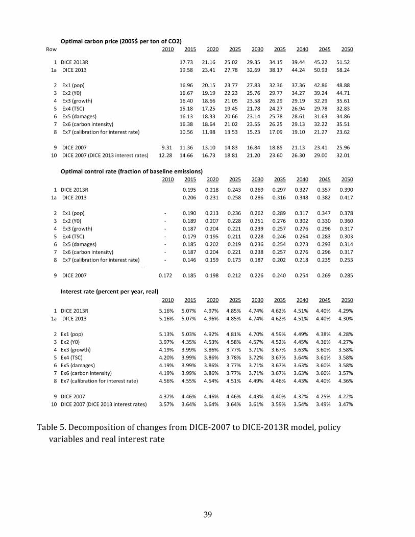
39

Table 5. Decomposition of changes from DICE-2007 to DICE-2013R model, policy

variables and real interest rate

Optimal carbon price (2005$ per ton of CO2)Row 2010 2015 2020 2025 2030 2035 2040 2045 2050

1 DICE 2013R 17.73 21.16 25.02 29.35 34.15 39.44 45.22 51.52

1a DICE 2013 19.58 23.41 27.78 32.69 38.17 44.24 50.93 58.24

2 Ex1 (pop) 16.96 20.15 23.77 27.83 32.36 37.36 42.86 48.88

3 Ex2 (Y0) 16.67 19.19 22.23 25.76 29.77 34.27 39.24 44.71

4 Ex3 (growth) 16.40 18.66 21.05 23.58 26.29 29.19 32.29 35.61

5 Ex4 (TSC) 15.18 17.25 19.45 21.78 24.27 26.94 29.78 32.83

6 Ex5 (damages) 16.13 18.33 20.66 23.14 25.78 28.61 31.63 34.86

7 Ex6 (carbon intensity) 16.38 18.64 21.02 23.55 26.25 29.13 32.22 35.51

8 Ex7 (calibration for interest rate) 10.56 11.98 13.53 15.23 17.09 19.10 21.27 23.62

9 DICE 2007 9.31 11.36 13.10 14.83 16.84 18.85 21.13 23.41 25.96

10 DICE 2007 (DICE 2013 interest rates) 12.28 14.66 16.73 18.81 21.20 23.60 26.30 29.00 32.01

Optimal control rate (fraction of baseline emissions)2010 2015 2020 2025 2030 2035 2040 2045 2050

1 DICE 2013R 0.195 0.218 0.243 0.269 0.297 0.327 0.357 0.390

1a DICE 2013 0.206 0.231 0.258 0.286 0.316 0.348 0.382 0.417

2 Ex1 (pop) - 0.190 0.213 0.236 0.262 0.289 0.317 0.347 0.378

3 Ex2 (Y0) - 0.189 0.207 0.228 0.251 0.276 0.302 0.330 0.360

4 Ex3 (growth) - 0.187 0.204 0.221 0.239 0.257 0.276 0.296 0.317

5 Ex4 (TSC) - 0.179 0.195 0.211 0.228 0.246 0.264 0.283 0.303

6 Ex5 (damages) - 0.185 0.202 0.219 0.236 0.254 0.273 0.293 0.314

7 Ex6 (carbon intensity) - 0.187 0.204 0.221 0.238 0.257 0.276 0.296 0.317

8 Ex7 (calibration for interest rate) - 0.146 0.159 0.173 0.187 0.202 0.218 0.235 0.253

-

9 DICE 2007 0.172 0.185 0.198 0.212 0.226 0.240 0.254 0.269 0.285

Interest rate (percent per year, real)

2010 2015 2020 2025 2030 2035 2040 2045 2050

1 DICE 2013R 5.16% 5.07% 4.97% 4.85% 4.74% 4.62% 4.51% 4.40% 4.29%

1a DICE 2013 5.16% 5.07% 4.96% 4.85% 4.74% 4.62% 4.51% 4.40% 4.30%

2 Ex1 (pop) 5.13% 5.03% 4.92% 4.81% 4.70% 4.59% 4.49% 4.38% 4.28%

3 Ex2 (Y0) 3.97% 4.35% 4.53% 4.58% 4.57% 4.52% 4.45% 4.36% 4.27%

4 Ex3 (growth) 4.19% 3.99% 3.86% 3.77% 3.71% 3.67% 3.63% 3.60% 3.58%

5 Ex4 (TSC) 4.20% 3.99% 3.86% 3.78% 3.72% 3.67% 3.64% 3.61% 3.58%

6 Ex5 (damages) 4.19% 3.99% 3.86% 3.77% 3.71% 3.67% 3.63% 3.60% 3.58%

7 Ex6 (carbon intensity) 4.19% 3.99% 3.86% 3.77% 3.71% 3.67% 3.63% 3.60% 3.57%

8 Ex7 (calibration for interest rate) 4.56% 4.55% 4.54% 4.51% 4.49% 4.46% 4.43% 4.40% 4.36%

9 DICE 2007 4.37% 4.46% 4.46% 4.46% 4.43% 4.40% 4.32% 4.25% 4.22%

10 DICE 2007 (DICE 2013 interest rates) 3.57% 3.64% 3.64% 3.64% 3.61% 3.59% 3.54% 3.49% 3.47%

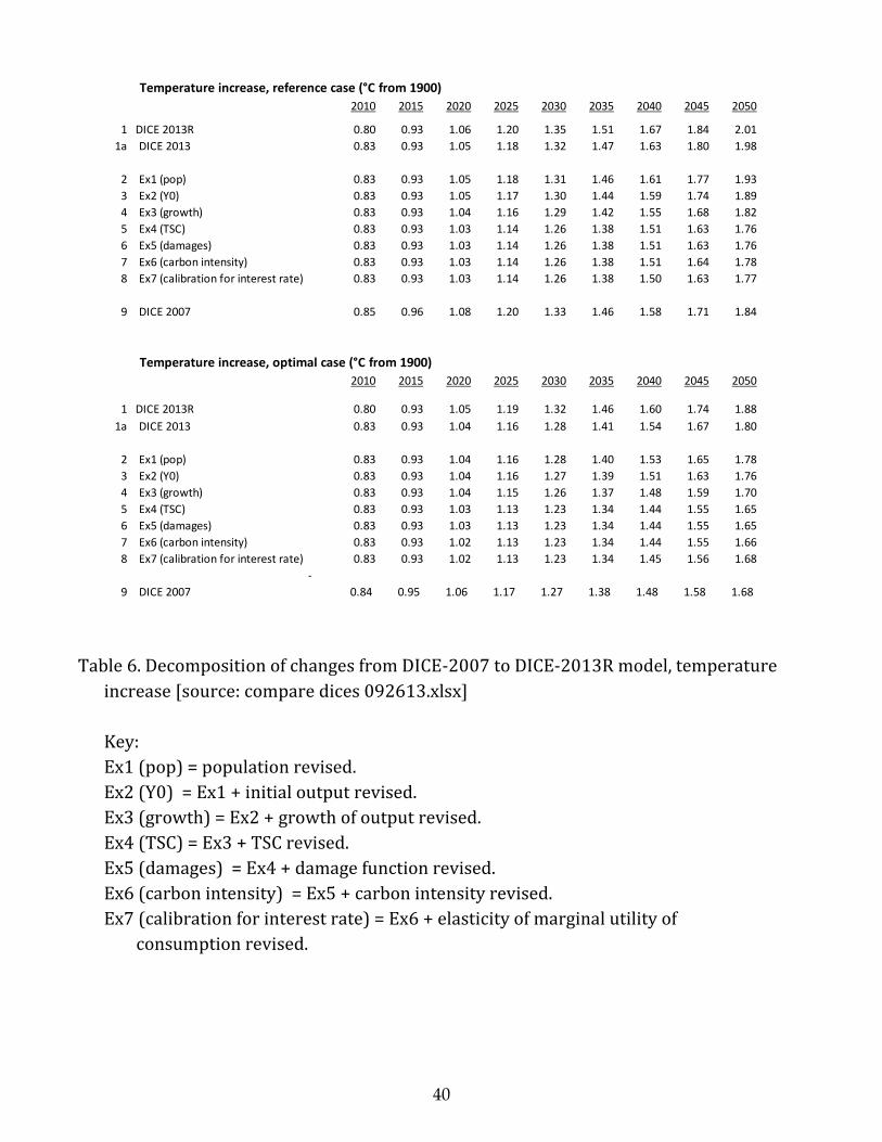
40

Table 6. Decomposition of changes from DICE-2007 to DICE-2013R model, temperature

increase [source: compare dices 092613.xlsx]

Key:

Ex1 (pop) = population revised.

Ex2 (Y0) = Ex1 + initial output revised.

Ex3 (growth) = Ex2 + growth of output revised.

Ex4 (TSC) = Ex3 + TSC revised.

Ex5 (damages) = Ex4 + damage function revised.

Ex6 (carbon intensity) = Ex5 + carbon intensity revised.

Ex7 (calibration for interest rate) = Ex6 + elasticity of marginal utility of

consumption revised.

Temperature increase, reference case (°C from 1900)

2010 2015 2020 2025 2030 2035 2040 2045 2050

1 DICE 2013R 0.80 0.93 1.06 1.20 1.35 1.51 1.67 1.84 2.01

1a DICE 2013 0.83 0.93 1.05 1.18 1.32 1.47 1.63 1.80 1.98

2 Ex1 (pop) 0.83 0.93 1.05 1.18 1.31 1.46 1.61 1.77 1.93

3 Ex2 (Y0) 0.83 0.93 1.05 1.17 1.30 1.44 1.59 1.74 1.89

4 Ex3 (growth) 0.83 0.93 1.04 1.16 1.29 1.42 1.55 1.68 1.82

5 Ex4 (TSC) 0.83 0.93 1.03 1.14 1.26 1.38 1.51 1.63 1.76

6 Ex5 (damages) 0.83 0.93 1.03 1.14 1.26 1.38 1.51 1.63 1.76

7 Ex6 (carbon intensity) 0.83 0.93 1.03 1.14 1.26 1.38 1.51 1.64 1.78

8 Ex7 (calibration for interest rate) 0.83 0.93 1.03 1.14 1.26 1.38 1.50 1.63 1.77

9 DICE 2007 0.85 0.96 1.08 1.20 1.33 1.46 1.58 1.71 1.84

Temperature increase, optimal case (°C from 1900)

2010 2015 2020 2025 2030 2035 2040 2045 2050

1 DICE 2013R 0.80 0.93 1.05 1.19 1.32 1.46 1.60 1.74 1.88

1a DICE 2013 0.83 0.93 1.04 1.16 1.28 1.41 1.54 1.67 1.80

2 Ex1 (pop) 0.83 0.93 1.04 1.16 1.28 1.40 1.53 1.65 1.78

3 Ex2 (Y0) 0.83 0.93 1.04 1.16 1.27 1.39 1.51 1.63 1.76

4 Ex3 (growth) 0.83 0.93 1.04 1.15 1.26 1.37 1.48 1.59 1.70

5 Ex4 (TSC) 0.83 0.93 1.03 1.13 1.23 1.34 1.44 1.55 1.65

6 Ex5 (damages) 0.83 0.93 1.03 1.13 1.23 1.34 1.44 1.55 1.65

7 Ex6 (carbon intensity) 0.83 0.93 1.02 1.13 1.23 1.34 1.44 1.55 1.66

8 Ex7 (calibration for interest rate) 0.83 0.93 1.02 1.13 1.23 1.34 1.45 1.56 1.68

-

9 DICE 2007 0.84 0.95 1.06 1.17 1.27 1.38 1.48 1.58 1.68

41

Here is the series of steps. The steps move backwards from the 2013R model to

the 2007 model.

Row 1. This is the optimized run for the DICE-2013R model.

Row 1a. This is the optimized run for DICE-2013 from April 2013. There are

several small differences from DICE-2013R, particularly initial conditions,

lowering the temperature sensitivity coefficient, and raising exogenous non-CO2

forcings. The change in the social cost of carbon is largely due to the lowering of

the temperature sensitivity.

Row 2. The population projection changes from the IIASA model to the UN

projections. This made little difference in the near term but increased the

asymptotic population from 8,600 to 10,500 million.

Row 3. The next correction is for the output level in 2010. The 2007 model

overpredicted output by about 6 percent, primarily because of failure to see the

Great Recession. We have reduced output to put the new path on the current

starting point.

Row 4. We have revised downward slightly the rate of growth of total factor

productivity over the coming decades. For example, projected world GDP for

2105 was revised upward from 1.55% per year to 2.23% per year. The

projection after 2105 was essentially unchanged.

Row 5. The temperature sensitivity coefficient (effect of doubling CO2

concentrations on equilibrium temperature) was increased from 3.0 °C to 3.2 °C

in the 2013 version. Row 5 shows the effect of reducing it back to the 2007

assumption.

Row 6. The damage function was recalibrated to correspond to the Tol survey,

which had slightly lower damages than the earlier DICE/RICE models. In row 6,

we increase the damage function to correspond to the DICE-2007 assumption.

Row 7. Emissions in 2010 were about 2.5% higher than were projected in the

2007 model. We therefore lowered the initial emissions intensity to correspond

to the 2007 estimate. Carbon intensity was projected to grow about 0.3% per

year more rapidly than the new projection. Row 7 shows the effect of going back

to the higher carbon intensity and the difference in initial emissions.

Row 8. The parameters of the utility function are set at the DICE-2007 level.

This increases the elasticity of the utility function from 1.45 to 2.

Row 9. Shows the results of the DICE-2007 model.

Row 10. This takes the DICE-2007 model and changes the consumption

elasticity from 2 to 1.45 to determine the effect of this parameter alone.

42

The results show that the optimal carbon price (and the social cost of carbon)

increased sharply from the 2007 model to the 2013R model, from $11.36 per ton of

CO2 to $17.73 per ton of CO2 in 2015, an increase of approximately 60%. Two

variables contributed most to this change: the calibration of interest rates and the

higher population growth. These contributed approximately equally to the increase

in the SCC.

All other variables individually made a modest difference, sometimes positive

and sometimes negative, but the other variables netted out to approximately zero. If

the two key variables are changed at the same time, the SCC is very close to the 2007

calculation ($11.53 v. $11.36). As noted above, the population revision reflects

moving from the IIASA projection to the UN projection. The change in the interest

rate is primarily due to a more careful calibration in the 2013 model with a specific

target real rate of interest explicitly targeted.

B. Revisions in the DICE model over the last two decades (*)

We have reviewed the revisions since the first published version of the DICE

model in Nordhaus (1992) as well as carbon prices since the earliest related model.

This review shows that model developments and revisions have had substantial

effects on the outcomes.

Figure 11 compares the projections of atmospheric CO2 concentrations of the

DICE-2013R model with several models of the EMF-22 comparison. The DICE-

2013R is higher in part because of projections of higher CO2 emissions and in part

because of higher atmospheric retention (see above).

43

Figure 11. Comparison of CO2 concentrations between DICE-2013R and EMF-

22 models

[Source: Clarke et al. (2009) and spreadsheet with results provided by Leon Clarke.

Manual_Figs_092713.xlsx, F8]

___________________

Figure 12 shows the projections of temperature increase. The earliest

vintages had an intermediate temperature projection. The projected change to 2100

decreased and then increased for the latest vintage. The earliest versions projected

2100 temperature increase of a little above 3 °C, whereas the latest version is a full

degree C above that. The increase is a combination of more rapid output growth,

higher temperature sensitivity, and a higher fraction of emissions retained in the

atmosphere.

300

400

500

600

700

800

900

1000

2000 2010 2020 2030 2040 2050 2060 2070 2080 2090 2100

Atm

osp

he

ric

con

cen

tra

tio

ns

(pp

m)

EMF: 10

EMF: 50

EMF: 90

DICE-2013R

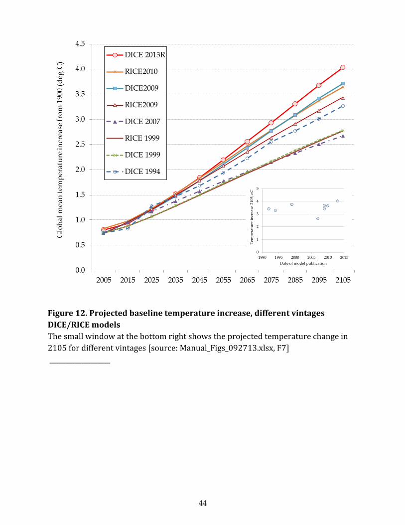
44

Figure 12. Projected baseline temperature increase, different vintages

DICE/RICE models

The small window at the bottom right shows the projected temperature change in

2105 for different vintages [source: Manual_Figs_092713.xlsx, F7]

___________________

0.0

0.5

1.0

1.5

2.0

2.5

3.0

3.5

4.0

4.5

2005 2015 2025 2035 2045 2055 2065 2075 2085 2095 2105

Glo

bal

mea

n t

emp

erat

ure

incr

ease

fro

m 1

900

(deg

C)

DICE 2013R

RICE2010

DICE2009

RICE2009

DICE 2007

RICE 1999

DICE 1999

DICE 1994

0

1

2

3

4

5

1990 1995 2000 2005 2010 2015

Tem

per

atu

re i

ncr

ease

21

05

, oC

Date of model publication

45

Figure 13 shows the damage-output ratio over the vintages. The estimated

damage-output has risen by about one-third over the different vintages. This is

primarily due to higher temperature projections .

Figure 13. Damages as percent of output, baseline, different vintages

DICE/RICE models

[Source: Manual_Figs_092713.xlsx; SF4n]

_____________________

Figure 15 shows the calculated optimal carbon prices for vintages of models

going back to the first unpublished study in 1975, looking at the estimated prices for

three different years. The prices have been put in comparable prices and concepts,

although some differences remain. The optimal price in 2013 is surprisingly close to

the first calculations even though the models have changed dramatically.3 This

3 The earliest calculation of an optimal carbon tax was in Nordhaus (1975). This calculated the price of keeping CO2 concentrations to a doubling, which is approximately the optimal path.

0

1

2

3

4

5

2005 2015 2025 2035 2045 2055 2065 2075 2085 2095 2105

Da

ma

ges

as

% o

f o

utp

ut

DICE 2007

RICE 2007

RICE 2008

RICE 2009

RICE 2009

RICE 2010

DICE 2013R

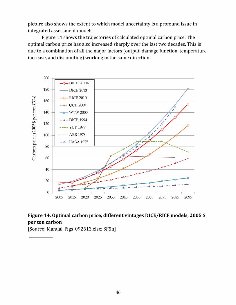
46

picture also shows the extent to which model uncertainty is a profound issue in

integrated assessment models.

Figure 14 shows the trajectories of calculated optimal carbon price. The

optimal carbon price has also increased sharply over the last two decades. This is

due to a combination of all the major factors (output, damage function, temperature

increase, and discounting) working in the same direction.

Figure 14. Optimal carbon price, different vintages DICE/RICE models, 2005 $

per ton carbon

[Source: Manual_Figs_092613.xlsx; SF5n]

_____________

0

20

40

60

80

100

120

140

160

180

200

2005 2015 2020 2025 2035 2045 2055 2065 2075 2085 2095

Ca

rbo

n p

rice

(2

00

5$

per

to

n C

O2)

DICE 2013R

DICE 2013

RICE 2010

QOB 2008

WTW 2000

DICE 1994

YUP 1979

AER 1978

IIASA 1975

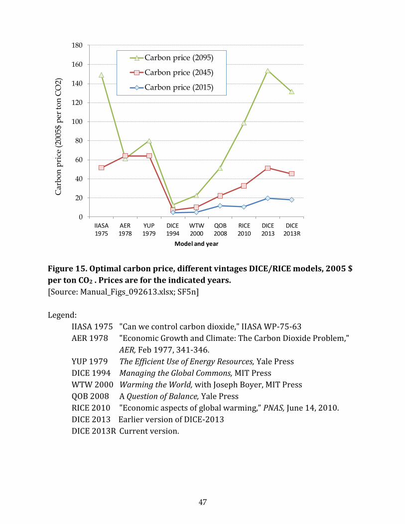
47

Figure 15. Optimal carbon price, different vintages DICE/RICE models, 2005 $

per ton CO2 . Prices are for the indicated years.

[Source: Manual_Figs_092613.xlsx; SF5n]

Legend:

IIASA 1975 "Can we control carbon dioxide," IIASA WP-75-63

AER 1978 "Economic Growth and Climate: The Carbon Dioxide Problem,"

AER, Feb 1977, 341-346.

YUP 1979 The Efficient Use of Energy Resources, Yale Press

DICE 1994 Managing the Global Commons, MIT Press

WTW 2000 Warming the World, with Joseph Boyer, MIT Press

QOB 2008 A Question of Balance, Yale Press

RICE 2010 "Economic aspects of global warming,” PNAS, June 14, 2010.

DICE 2013 Earlier version of DICE-2013

DICE 2013R Current version.

0

20

40

60

80

100

120

140

160

180

IIASA1975

AER1978

YUP1979

DICE1994

WTW2000

QOB2008

RICE2010

DICE2013

DICE2013R

Car

bo

n p

rice

(20

05$

per

to

n C

O2)

Model and year

Carbon price (2095)

Carbon price (2045)

Carbon price (2015)

48

VIII. Computational and algorithmic aspects (*)

A. Analytical background (*)

As we discuss in the next section, IAMs are generally computationally

complex compared to physical science models, such as climate models, that use

recursive time-stepped algorithms. Among IAMs, the DICE model is relatively simple

because it is a straightforward non-linear optimization problem. The DICE model

has generally been solved using the CONOPT or NLP solver in the GAMS modeling

system (see Brooke et al. 2005). This is based on the generalized reduced gradient

(GRG) algorithm. The details of the algorithm are available in the user manual for

the CONOPT solver.

CONOPT is generally a local solver and cannot ensure that the solution is a

global optimum. However, the DICE-2013R version has also been solved using the

BARON solver, which determines whether the solution is a global optimum. The

BARON solver is slower than the CONOPT or other local solvers, but can solve most

examples within a minute or so. A number of runs of different versions (Base,

Optimal, as well as a version with a highly concave-convex damage function)

indicates that the solutions with CONOPT are in all examined cases also the global

optima.

Over the last decade, we have also used the EXCEL Solver (using the Risk

Solver Platform or other premium product). This has the major advantage that

optimization can be performed over prices, which is a natural approach for global

warming economics. It is very difficult to implement a solution using prices as a

decision variable in a standard linear programming algorithm. If the prices can be

solved analytically, as is the case with the current DICE model, then prices can be

used as a solution variable, but only as an implicit variable. Using EXCEL Solver is

also much easier to understand and to detect programming errors. It is also easier

to use Excel when introducing new variables and models as the graphics can be

employed to find problems. Recent versions of GAMS using auxiliary software such

as “R” makes graphics easier but still cumbersome. EXCEL has the shortcoming of

having much longer and more complex coding.

By contrast with the DICE model, the RICE model (with multiple optimizing

agents in equilibrium) is conceptually a fixed point problem. Many integrated

assessment models today use a Negishi algorithm to solve this, and this is the

approach followed in the RICE solutions. The origins of the Negishi approach date

from work of Takashi Negishi, Alan Manne, Peter Dixon, Victor Ginsberg and Jean

Waelbroeck, and Thomas Rutherford. The Negishi theorem is essentially an

application of the second theorem of welfare economics. Several authors

49

implemented this in the mid-1990s, particularly Nordhaus and Yang (1996) in the

first version of the RICE model, although the actual implementations were and

continue to differ among IAMs.

The RICE-2010 model has been implemented only in the Excel format. The

baseline RICE-2010 model can be used by researchers and students in the Excel

format and need not rely upon Solver. However, the full optimization requires the

advanced proprietary versions of Solver.4 We hope to develop a new version of the

RICE model in the near future.

It should also be noted that Excel Solver is unable to solve the largest version

of the RICE model in a reliable fashion, and errors sometimes occur when using

Solver. Even for the DICE model, Excel Solver is unreliable. For example, when using

the Solver to optimize the solution for reaching a global optimum for limiting

temperature to 2 °C, different starting points yield optimal carbon prices that differ

substantially for the first few periods when tolerances are set at their maximum. In

some circumstances, Solver simply balks and cannot find a solution, and sometimes

it finds a wildly incorrect solution.

B. Solution concepts (*)

We can summarize the points in this section in one paragraph: The DICE model

is relatively simple compared to many integrated assessment models. Nonetheless,

solving the model—particularly when optimizing emissions reductions – requires

modern algorithms for solving non-linear optimization problems. The current DICE

model is available in two different platforms. The simplest one is Excel Risk Solver

Platform (available for $640 to academic users). The second platform is the GAMS

software system (General Algebraic Modeling System). This can be accessed only

with proprietary software (available to academics for around $1000). For those who

have limited research budgets, the Excel version is the most convenient platform.

Here is a more complete discussion: Optimization IAMs are generally

computationally complex compared to physical science models, such as climate

models, that use recursive time-stepped algorithms. Optimization problems are

computationally complex because (from a mathematical point of view) they require

solving a set of equilibrium conditions, such as first-order conditions. While some

optimization problems can be solved quickly and efficiently, in general the

computational costs rise as a polynomial or exponential function of the number of

4 Those who wish to use the simple (free) version of Solver can use the Excel versions by simplifying the constraints and optimizing variables. For example, if a small number of variables are optimized, the free version can be used. While the present author has used that on occasions, there is no available version at present.

50

variables. By contrast, recursive problems (such as climate models) are linear in the

number of variables.

The DICE model traditionally was solved using the GAMS modeling system (see

Brooke et al. 2005). GAMS is a high-level modeling system for mathematical

programming and optimization. It contains a high-level language and several high-

performance solvers. We usually employ NLP solver in solving the DICE-RICE

models. This is based on the generalized reduced gradient (GRG) algorithm. This is

an algorithm that in practice has proven very efficient at solving large non-linear

optimization problems where the constraints are smooth. If the model is

“almost linear,” it can use inner linear-programming-like iterations to achieve a

rapid solution.

In the latest round of models, we have used the EXCEL Solver (using the Risk

Solver Platform or other premium product). This has the several advantages. One is

that optimization can be performed over prices, which is a natural approach for

global warming economics. (It is difficult to implement a solution using prices as a

decision variable in a standard linear programming algorithm.) Using EXCEL Solver

is also much easier to understand and to detect programming errors. Note that if the

price can be solved analytically, it can be used as a control variable in GAMS (which

is the case in the most recent version of GAMS).

By contrast, the RICE model (with multiple optimizing agents in equilibrium) is

conceptually a fixed point problem. Most integrated assessment models today use a

Negishi algorithm to solve this, and this is the approach followed in the RICE

solutions. The origins of the Negishi approach date from work of Takashi Negishi,

Peter Dixon, Victor Ginsberg and Jean Waelbroeck, Thomas Rutherford, and

Rutherford and Manne. The Negishi theorem is essentially an application of the

second theorem of welfare economics. Several authors implemented this in the mid-

1990s, particularly Nordhaus and Yang (1996) in the first version of the RICE model,

although the actual implementations were and continue to differ among IAMs.

One disadvantage of the Excel solvers is that they have trouble with large

problems and are often unreliable. For example, when using the Solver to optimize

the solution for reaching a global optimum for limiting temperature to 2 °C, different

starting points yield optimal carbon prices that differ substantially. In some

circumstances, Solver simply stops and cannot find a solution, and sometimes it

finds a wildly incorrect solution.

A compendium of studies in several areas with many illuminating articles of

CGE modeling is contained in Dixon and Jorgenson (2012).

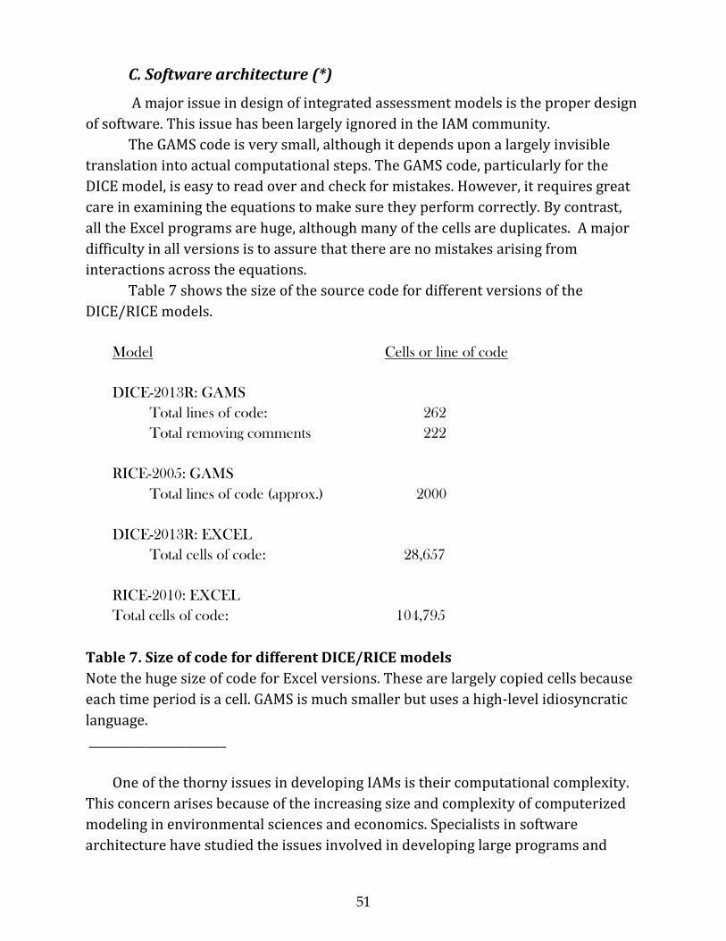
51

C. Software architecture (*)

A major issue in design of integrated assessment models is the proper design

of software. This issue has been largely ignored in the IAM community.

The GAMS code is very small, although it depends upon a largely invisible

translation into actual computational steps. The GAMS code, particularly for the

DICE model, is easy to read over and check for mistakes. However, it requires great

care in examining the equations to make sure they perform correctly. By contrast,

all the Excel programs are huge, although many of the cells are duplicates. A major

difficulty in all versions is to assure that there are no mistakes arising from

interactions across the equations.

Table 7 shows the size of the source code for different versions of the

DICE/RICE models.

Model Cells or line of code

DICE-2013R: GAMS

Total lines of code: 262

Total removing comments 222

RICE-2005: GAMS

Total lines of code (approx.) 2000

DICE-2013R: EXCEL

Total cells of code: 28,657

RICE-2010: EXCEL

Total cells of code: 104,795

Table 7. Size of code for different DICE/RICE models

Note the huge size of code for Excel versions. These are largely copied cells because

each time period is a cell. GAMS is much smaller but uses a high-level idiosyncratic

language.

________________________

One of the thorny issues in developing IAMs is their computational complexity.

This concern arises because of the increasing size and complexity of computerized

modeling in environmental sciences and economics. Specialists in software

architecture have studied the issues involved in developing large programs and

52

emphasize the difficulties of ensuring that software is reliable and well-tested. A

rule of thumb is that well-developed software contains in the order of 1 error per

source line of code (SLOC). Since many computerized climate and integrated

assessment models contain between 10,000 and 1 million SLOC, there is the

prospect of many bugs contained in our code. 5

This proposition is not just theoretical. There are many examples of

catastrophically bad software, such as the errors that led to the crashing of a

spacecraft because of insertion of a period instead of a comma in a FORTRAN

statement; or inappropriate shutdown of five nuclear power reactors because of an

incorrect formula programmed. Current luxury automobiles have millions of lines of

code and probably contain untold thousands of bugs.

I take it as a given that large IAMs have a variety of errors, some consequential,

some not. I did a routine check of one of my large models (the RICE 2011 in

development at the time). I found a high error rate in terms of stranded code, poor

definitions, and mistaken references. For the lines I examined, there were no

substantive mistakes, but I suspect that had I gone further some would have turned

up. In the RICE-2010 version, there was a mistaken reference in the sea-level rise

module that led to small errors in the numerical projections. This was discovered by

an interested user and corrected. Another example of coding issues was from the

OECD Green model (discussed in Nordhaus (2012).

I will explore one error in depth because it is so subtle that it was found only

after an intensive examination. The FUND model is one of the leading models used

by researchers and governments to understand the economics of global warming. It

has been used to calculate the social cost of carbon for the U.S., which calculation

affects tens of billions of dollars of regulations.

The problem with the FUND model arose because of a formula for one of the

components of the damage function in an early version (since corrected). The

specification had agricultural damages, which were calculated with a formula having

a normal variable in both the numerator and the denominator. This looks

unnecessarily complex but innocuous. In fact, it turned out to be a serious error.

This was pointed out in an article by Ackerman and Munitz (2012), which made the

following statement: “The manner in which the optimum temperature effect is

modeled in FUND 3.5 could cause division by zero for a plausible value of a Monte

Carlo parameter.” 5 This section draws on a lecture presented at the Prague meetings of the EAREA in June 2012 and the debate about software design that ensued after that. References are contained in that discussion.

53

It will be useful to examine the issue from a statistical point of view. The

details are the following: In FUND 3.5, according to the model description, the

damages for the level of temperature on agriculture have two terms. The first term

of the damage component can be written as y = az/(b-z)T, where y = damages, T =

temperature (an endogenous variable); a and b are parameters ; and z is a random

variable, which in the FUND model is (T-Topt,r). The variable Topt,r represents the

optimal temperature in region r and is a normally distributed random variable, so y

is the ratio of two normal variables.

The ratio of two normal distributions with non-zero means is a non-central

Cauchy distribution. A non-central Cauchy distribution has a standard Cauchy term

and another complicated term, but we can focus on the Cauchy term. This

distribution is “fat tailed” and has both infinite mean and infinite variance. So the

damages from agriculture in FUND 3.5 (from a statistical point of view) will

dominate both the mean and dispersion of the estimated damages. Taken literally,

the expected value of damages to agriculture are infinite at every temperature

increase. This is subject to sampling error in finite samples of any size, but the

sampling error is infinite since the moments do not exist, so any numerical

calculations with finite samples are (infinitely) inaccurate. There is also a coding

issue because it is not possible to get an accurate estimate of the distribution of a

variable with infinite mean and variance in finite samples. The most troubling

impact of this specification is the estimate of the distribution of outcomes (such as

the social cost of carbon or SCC). If the damages are a fat tailed distribution, then the

SCC is also fat- tailed. In finite samples, of course, all the moments are finite, but the

estimates are unreliable or fragile and depend upon the sample.

I assume that this strange distribution was not intended, and in any case is

easily corrected. My point was not to dwell on the shortcomings of our models.

Rather, we need to recognize that most economists and environmental scientists are

amateurs at software design and architecture. As computers get faster, as software

packages get more capable, as our theories get more elaborate – there is a tendency

to develop models that increase in parallel with the rapidly expanding frontier of

computational abilities. This leads to increasingly large and complex models. We

need also to ask, do we fully understand the implication of our assumptions? Is

disaggregation really helping or hurting?

There is another lesson here about uncertainty analyses. Deterministic IAMss

are already complex non-linear systems. Introducing uncertainty through a set of

complicated functions of random variables adds yet another layer of complexity.

Modelers need to be especially careful that they have not changed the properties

and outcomes of the models because of strange behavior or interactions of the

54

added random variables. The properties of linear stochastic systems are moderately

well-understood, but that is not the case for all non-linear stochastic systems.

The conclusions here are four and apply to the DICE/RICE and other large IAMs.

First, we modelers need to recognize the importance of good software architecture.

Second, we should restrain the urge to develop ever larger and more complex

computational models unless there is a clear and convincing case that they will

improve our understanding or are necessary to understand the phenomena at hand.

Third, we need to undertake special scrutiny when we add random elements to non-

linear dynamic models. Finally, we need to take the extra time and effort to examine,

re-examine, and test our software.

IX. Conclusion (*)

The present manual is intended to provide users as well as those interested in

integrated assessment modeling a self-contained document for understanding and

using the DICE/RICE family of models.

As with all large-scale models of this kind, they must be continuously updated.

Additionally, they are prone to errors in the software and structure, data and

scientific views evolve, and users must be attentive to the potential for large and

small changes in the economics and natural sciences. Problems arise particularly

when modifications are made to models (such as alternative parameterizations) and

the model is not carefully tested to make sure that the changes do not alter the

behavior or introduce instabilities.

The DICE model has evolved significantly over the years since its

development. The vast changes in the projections of different variables might lead

some to conclude that these undermine the credibility of the modeling approach.

My response would be different, however, and can best be summarized by a

remark made in another context. The economist John Maynard Keynes was

criticized for changing his views on monetary policy during the Great Depression.

His response is reported to be, “When the facts change, I change my mind. Pray, sir,

what do you do?” This is a reminder of the need to be constantly attentive to

changing economic and scientific findings. Even more important is to resist getting

dug into a Maginot Line defense of particular views or projections. To err is human,

so to be humble is divine.

55

X. References

Ackerman, Frank, Elizabeth A. Stanton, Ramón Bueno (2010). “Fat tails, exponents, extreme

uncertainty: Simulating catastrophe in DICE,” Ecological Economics 69, 1657–1665.

Ackerman, Frank and Charles Munitz, “Climate damages in the FUND model: A

disaggregated analysis,” Ecological Economics.

Arrow, Kenneth J. (1962). “Economic Welfare and the Allocation of Resources for Invention,”

in Richard Nelson, The Rate and Direction of Inventive Activity, Princeton University Press

for National Bureau of Economic Research.

Arrow, Kenneth J. et al. (1995). Intertemporal equity, discounting, and economic efficiency,

in Climate Change 1995: Economic and Social Dimensions of Climate Change, Contribution

of Working Group III to the Second Assessment Report of the Intergovernmental Panel on

Climate Change, eds. Bruce J, Lee H, Haites E, Cambridge University Press, Cambridge, UK.

pp. 125–44.

Baranzini, Andrea, Marc Chesney, and Jacques Morisset (2003). “The impact of possible

climate catastrophes on global warming policy,” Energy Policy, Vol. 31, Issue 8, June, Pages

691-701.

Barrett, Scott (1994). Self-enforcing international environmental agreements. Oxford

Economic Papers 46, pp. 878–894.

Barrett, Scott (2003). Environment and Statecraft: The Strategy of Environmental Treaty-

Making. Oxford: Oxford University Press.

Bosetti, V., Carraro, C., Tavoni, M. (2009). “Climate change mitigation strategies in fast-

growing countries: the benefits of early action,” Energy Economics,,31, S144–S151.

Brooke, Anthony, David Kendrick, Alexander Meeraus, and Ramesh Raman (2005). GAMS: A

Users Guide, GAMS Development Corporation, Washington, D.C.

Carraro, C. and Siniscalco, D. (1993). “Strategies for the international protection of the

environment,” Journal of Public Economics, 52, pp. 309–328.

Cass, David (1965). “Optimum Growth in an Aggregative Model of Capital Accumulation,”

Review of Economic Studies. 32(3): 233–240.

56

Chander, P. and Tulkens, H. (1995). “A core-theoretical solution for the design of

cooperative agreements on trans-frontier pollution,” International Tax and Public Finance,

2, pp. 279–294.

Clarke L., C. Böhringer T.F. Rutherford (2009), “International, U.S. and E.U. climate change

control scenarios: Results from EMF 22,” Energy Economics, 31 (Suppl 2), pp. S63-S306.

Cline, William (1992). The Economics of Global Warming, Institute for International

Economics, Washington, D.C.

CONAES (1980). Committee on Nuclear and Alternative Energy Systems,

Energy in Transition, 1985-2010: Final Report of the Committee on Nuclear and Alternative

Energy Systems, National Research Council, 1980.

Cropper, Maureen (1976). “Regulating Activities with Catastrophic Environmental Effects,”

Journal of Environmental Economics and Management, 3, l-15.

EPPA (2011). Economics, Emissions, and Policy Cost - The EPPA Model, available at

http://globalchange.mit.edu/igsm/eppa.html.

Peter Dixon and Dale Jorgenson, eds. (2012). Handbook of Computable General Equilibrium

Modeling, two volumes, Elsevier, Amsterdam.

Epstein, L. and S. Zin (1989). “Substitution, Risk Aversion and the Temporal Behavior

of Consumption and Asset Returns: A Theoretical Framework,” Econometrica, 57, 937-969.

Epstein, L. and S. Zin (1991). “Substitution, Risk Aversion and the Temporal Behavior of

Consumption and Asset Returns: An Empirical analysis,” Journal of Political Economy, vol.

99, 263-288.

Gillingham, Kenneth, Richard G. Newell, and William A. Pizer (2008). “Modeling

endogenous technological change for climate policy analysis,” Energy Economics, Volume

30, Issue 6, pp. 2734-2753

Gordon, Robert B., Tjalling Koopmans, William Nordhaus, and Brian Skinner (1987).

Toward a new Iron Age? Quantitative modeling of resource exhaustion, Harvard University

Press, Cambridge, Mass.

Goulder, Lawrence (2002). Environmental policy making in economies with prior tax

distortions, Cheltenham, UK: Edwin Elgar.

57

Greenstone, Michael, Elizabeth Kopits, and Ann Wolverton (2011)”Estimating the social

cost of carbon for use in U.S. federal rulemakings: A summary and interpretation,” NBER

Working Paper 16913.

Hansen, James, Makiko Sato, Reto Ruedy, Ken Lo, David W. Lea, and Martin Medina-Elizade

(2006). “Global temperature change,” Proceedings of the National Academy of Sciences, USA,,

103: 14288-14293.

Hope, Chris (2006). “The marginal impact of CO2 from PAGE2002: an integrated

assessment model incorporating the IPCC's five reasons for concern,” Integrated

Assessment, vol. 6, pp. 19-56.

Hotelling, Harold (1931). “The economics of exhaustible resources,” Journal of Political

Economy, 39: 137-175.

IGEM (2011). Documentation for Intertemporal General Equilibrium Model (IGEM), available

at http://www.igem.insightworks.com/.

IIASA World Population Program (2007). Probabilistic Projections by 13 world regions,

forecast period 2000-2100, 2001 Revision, online at

http://www.iiasa.ac.at/Research/POP/proj01/.

Intergovernmental Panel on Climate Change (2007). Climate Change 2007: Mitigation of

Climate Change, Working Group III Contribution to the Intergovernmental Panel on Climate

Change (Cambridge Univ Press, Cambridge, UK).

International Monetary Fund (2009). World Economic and Financial Surveys, World

Economic Outlook Database, IMF, Washington.

International Monetary Fund (2007). World Economic and Financial Surveys, World

Economic Outlook Database, September 2006 Edition, available online at

http://www.imf.org/external/pubs/ft/weo/2006/02/data/index.aspx .

IPCC Fifth Assessment, Science (2013). Intergovernmental Panel on Climate Change,

Climate Change 2013: The Physical Science Basis, Contribution of Working Group I to the

Fourth Assessment Report of the IPCC, available online at

http://www.ipcc.ch/report/ar5/wg1/#.Ukn99hCBm71.

IPCC Fourth Assessment, Impacts (2007). Intergovernmental Panel On Climate Change,

Climate Change 2007: Impacts, Adaptation and Vulnerability, Working Group II Contribution

58

to the Intergovernmental Panel on Climate Change, Summary for Policymakers, April,

available online at http://www.ipcc.ch/.

IPCC Fourth Assessment, Mitigation (2007). Intergovernmental Panel on Climate Change,

Climate Change 2007: Mitigation of Climate Change, Working Group III Contribution to the

Intergovernmental Panel on Climate Change, available online at http://ipcc-

wg1.ucar.edu/wg1/wg1-report.html.

IPCC Fourth Assessment, Science (2007). Intergovernmental Panel on Climate Change,

Climate Change 2007: The Physical Science Basis, Contribution of Working Group I to the

Fourth Assessment Report of the IPCC, available online at http://ipcc-

wg1.ucar.edu/wg1/wg1-report.html.

IPCC Second Assessment, Economics (1996). Climate Change 1995—Economic and Social

Dimensions of Climate Change. Eds. Bruce J., H. Lee, and E. Haites. Cambridge, UK:

Cambridge University Press.

IPCC SRES (2000). Special Report on Emissions Scenarios, The Intergovernmental Panel on

Climate Change, Cambridge University Press, Cambridge, UK.

IPCC Third Assessment, Science (2001). Contribution of Working Group I to the Third

Assessment Report of the Intergovernmental Panel on Climate Change. Climate Change

2001: The Scientific Basis. Ed. J. T. Houghton, Y. Ding, D.J. Griggs, M. Noguer, P. J. van der

Linden, and D. Xiaosu, Cambridge: Cambridge University Press.

Kelly, David L. and Charles D. Kolstad (1999). “Integrated Assessment Models For Climate

Change Control,” In International Yearbook of Environmental and Resource Economics

1999/2000: A Survey of Current Issues, ed. Henk Folmer and Tom Tietenberg. Cheltenham,

UK: Edward Elgar.

Knutti, Reto and Gabriele Hegerl (2008). “The equilibrium sensitivity of the Earth's

temperature to radiation changes,” Nature Geoscience 1, 735 – 743.

Kolstad, Charles D. (1996). “Learning And Stock Effects In Environmental Regulation: The

Case Of Greenhouse Gas Emissions, Journal Of Environmental Economics And Management,

31, 1-18.

Koopmans Tjalling (1963). “On the concept of optimal economic growth,” Cowles

Foundation Discussion Papers. Yale Univ. Available at

http://cowles.econ.yale.edu/P/cd/d01b/d0163.pdf.

59

Koopmans, Tjalling C. (1965). “On the Concept of Optimal Economic Growth,” Academiae

Scientiarum Scripta Varia 28(1): 1-75 (available for download at

http://cowles.econ.yale.edu/P/au/p_koopmans.htm).

Lee, Ronald (2011). “The Outlook for Population Growth,” Science, Vol. 333 no. 6042, pp.

569-573.

Lind, Robert C. (1995). “Intergenerational equity, discounting, and the role of cost-benefit

analysis in evaluating global climate policy,” Energy Policy,

Vol. 23, Issues 4-5, April-May, pp. 379-389.

Lind, Robert C. and F. R. Ruskin, eds. (1982). Discounting for time and risk in energy policy,

Resources for the Future, Inc., Washington, DC.

Manne, Alan S. (1962). “Product-Mix Alternatives: Flood Control, Electric Power, and

Irrigation, International Economic Review, Vol. 3, No. 1, Jan., pp. 30-59

Manne, Alan S. (1974). “Waiting for the Breeder,” The Review of Economic Studies, Vol. 41,

Symposium on the Economics of Exhaustible Resources (1974), pp. 47-65.

Manne, Alan S. (1976). “ETA: A Model for Energy Technology Assessment,” Bell Journal of

Economics, Vol. 7, No. 2, Autum, pp. 379-406.

Manne, Alan S. (1985). “On the Formulation and Solution of Economic Equilibrium

Problems,” Mathematical Programming Study, 23, pp. 1-23.

Manne, A. and Richels, R. (1991). “Global CO2 Emission Reductions; the Impacts of Rising

Energy Costs,” The Energy Journal, vol. 12(1), pp. 87-108.

Manne, Alan S. and Richard G. Richels (1992). Buying Greenhouse Insurance: The Economic

Costs of Carbon Dioxide Emission Limits, MIT Press, Cambridge, MA, 1992.

Manne, Alan S. and Richard Richels (1999). “The Kyoto Protocol: A Cost-Effective Strategy

for Meeting Environmental Objectives?” In The Costs of the Kyoto Protocol: a Multi-model

Evaluation, ed. John Weyant and Jennifer Hill. The Energy Journal, Special edition: 1-24.

Manne, Alan S. and Richels, Richard G (2001). “U.S. Rejection of the Kyoto Protocol: The

Impact on Compliance Costs and CO2 Emissions,” AEI-Brookings Joint Center Working

Paper No. 01-12.

60

Manne, Alan S. and Richard G. Richels (2004). “MERGE: An Integrated Assessment Model

for Global Climate Change,” Stanford University, available at

http://www.stanford.edu/group/MERGE/GERAD1.pdf.

McKibbin, Warwick J., David Pearce, and Alison Stegman (2007). “Long term projections of

carbon emissions,” International Journal of Forecasting, 23(4), October-December: 637-653.

Mehra, Rajnish (2008). The Handbook of the Equity Risk Premium, ed., Elsevier, Amsterdam,

2008, pp. 1-36.

MRG (1978). Report of the Modeling Resource Group of the Committee on Nuclear and

Alternative Energy Systems, Energy Modeling for an Uncertain Future, National Academy of

Sciences Press, 1978.

Nash, John (1950). “Equilibrium points in n-person games,” Proceedings of the National

Academy of Sciences, 1950, 36(1), pp. 48-49.

National Research Council (1992). Committee on Science, Engineering, and Public Policy,

Policy Implications of Greenhouse Warming: Mitigation, Adaptation, and the Science Base,

National Academy Press, Washington, D.C.

National Research Council, Committee on Abrupt Climate Change (2002),

Abrupt Climate Change: Inevitable Surprises, National Academy Press, Washington, D.C.

Nelson, Richard R. (1959). “The Simple Economics of Basic Scientific Research,” Journal of

Political Economy, vol. 67, pp.297-306.

NEMS (2011). The National Energy Modeling System: An Overview, available at

http://205.254.135.24/oiaf/aeo/overview/.

Nordhaus, William D. (1975). “Can We Control Carbon Dioxide?” Working Paper of the

International Institute for Systems Analysis, Laxenburg, Austria, WP-75-63.

Nordhaus, William D. (1977). “Economic Growth and Climate: The Carbon Dioxide

Problem,” The American Economic Review, 67, 1, pp. 341-346.

Nordhaus, William D. (1979). The Efficient Use of Energy Resources , Yale University Press,

New Haven, CT, USA.

61

Nordhaus, William D. (1992). “An Optimal Transition Path for Controlling Greenhouse

Gases,” Science, vol. 258, November 20, pp. 1315-1319.

Nordhaus, William D. (1994). Managing the Global Commons: The Economics of Climate

Change, MIT Press, Cambridge, MA, USA.

Nordhaus, William D. (1994a). “Expert Opinion on Climatic Change,” American Scientist,

January-February 1994, vol. 82, pp. 45-51.

Nordhaus, William D. (2002). “Modeling induced innovation in climate-change policy,” in

Technological Change and the Environment, edited by A. Grübler, N. Nakicenovic and W. D.

Nordhaus. Washington, DC: Resources for the Future, pp. 182–209

Nordhaus, William D. (2007). “The Stern Review on the Economics of Climate Change,”

Journal of Economic Literature, vol. 45, no. 3, pp. 686–70.2

Nordhaus, William D. (2007a). “Alternative measures of output in global economic-

environmental models: Purchasing power parity or market exchange rates?” Energy

Economics, 29, 3, pp. 349-372.

Nordhaus, William D. (2008). A Question of Balance: Weighing the Options on Global

Warming Policies, Yale University Press, New Haven, CT.

Nordhaus, William D. (2010). Economic aspects of global warming in a post-Copenhagen

environment. Proceedings of the U.S. National Academy of Sciences 107 (26), 11721-11726.

Nordhaus, William. (2011). “The Economics of Tail Events with an Application to Climate

Change,” Review of Environmental Economics and Policy, 5(2), pp. 240-257.

Nordhaus, William D. (2011a). “Estimates of the Social Cost of Carbon: Background and

Results from the RICE-2011 Model,” New Haven, CT. USA: Cowles Foundation Discussion

Paper.

Nordhaus, William D. (2011b). “Economic Policy in the Face of Severe Tail Events,” Journal

of Public Economic Theory, 14 (2), 2012, pp. 197–219.

Nordhaus, William D. (2012). “Integrated Economic and Climate Modeling,” Handbook of

Computable General Equilibrium Modeling, Peter Dixon and Dale Jorgenson, eds., Elsevier.

Nordhaus, William D. (2013). The Climate Casino: Risk, Uncertainty, and Economics of Global

Warming, Yale University Press, New Haven, CT.

62

Nordhaus, William D. and David Popp (1997). “What is the Value of Scientific Knowledge?

An Application to Global Warming Using the PRICE Model,” The Energy Journal, Vol. 18, No.

1, pp. 1-45.

Nordhaus, William D. and Joseph Boyer (2000). Warming the World: Economic Modeling of

Global Warming, MIT Press, Cambridge, MA., USA.

Nordhaus, William D. and Zili Yang (1996). “A Regional Dynamic General-Equilibrium

Model of Alternative Climate-Change Strategies,” American Economic Review, 86: 741-765.

Oakland, William H. (1987). ” Theory of public goods,” in Alan J. Auerbach and Martin

Feldstein, eds. Handbook of Public Economics, Volume 2, pp. 485-535.

David Pearce (2003). “The Social Cost of Carbon and its Policy Implications,” Oxford Review

of Economic Policy, 19 (3): 362-384.

Christos Papadimitriou (1994). “On the complexity of the parity argument and other

inefficient proofs of existence,” Journal of Computer and System Sciences, 48 (3), pp. 498–

532.

Peck, Stephen C. and Thomas J. Teisberg (1993), “Global Warming Uncertainties and the

Value of Information: An Analysis Using CETA,” Resource and Energy Economics, Vol. 15, No.

1, March 1993, pp. 71-97.

Peck, Stephen C. and Thomas J. Teisberg (1999). “CO2 concentration limits, the costs and

benefits of control and the potential for international agreements,”in Carraro, C., Editor,

1999. International Environmental Agreements on Climate Change, Kluwer Academic

Publishers, Dordrecht.

Pizer, William A. (1999). “Optimal Choice of Climate Change Policy in the Presence of

Uncertainty,” Resource and Energy Economics, 21: 255-287.

Point Carbon (2006). Historical prices. http://www.pointcarbon.com (accessed November

9, 2006 by subscription).

Popp, David (2004). “ENTICE: endogenous technological change in the DICE model of

global warming,” Journal of Environmental Economics and Management, 48: 742–68.

Portney, Paul R. and John P. Weyant, Eds. (1999). Discounting and Intergenerational Equity,

Washington, Resources for the Future, 1999.

63

Ramsey, Frank P. (1928). “A Mathematical Theory of Saving,” Economic Journal, 38(152):

543–559.

Rogelj, Joeri et al. (2010). “Copenhagen Accord pledges are paltry,” Nature, 464, 1126–

1128, 22 April 2010, doi:10.1038/4641126a

Romer, Paul (1990), “Endogenous Technological Change,” Journal of Political Economy, vol.

98, October, part 2, pp. S71-S102.

Rutherford TF (2009). "Extensions of GAMS for complementarity problems arising in

applied economics", Journal of Economic Dynamics and Control, December.

Samuelson, Paul A. (1954). “The pure theory of public expenditure.” Review of Economics

and Statistics, 36 (4): 387–389.

Samuelson, Paul A. (1949). Market mechanisms and maximization, Rand Corporation, P-49,

March 28, Santa Monica, CA.

Solow, R. M. (1970). Growth theory: an exposition, Oxford University Press, Oxford, UK.

SRES (2000). Nebojsa Nakicenovic et al. IPCC Special Report on Emissions Scenarios,

Intergovernmental Panel on Climate Change, available at

http://www.grida.no/publications/other/ipcc_sr/?src=/climate/ipcc/emission/.

Stern Review (2007). The Economics of Climate Change: The Stern Review, Cambridge

University Press, Cambridge, UK and available on the web at http://www.hm-

treasury.gov.uk/independent_reviews/stern_review_economics_climate_change/

sternreview_index.cfm.

Tol, R.S.J. (2003). “Is the Uncertainty about Climate Change Too Large for Expected Cost-

Benefit Analysis?” Climatic Change, vol. 56, no. 3, pp. 265-289.

Tol, R.S.J. (2005), “The Marginal Damage Costs of Carbon Dioxide Emissions: An

Assessment of the Uncertainties”, Energy Policy, 33, 2064-2074.

Tol, R.S.J. (2008). “The Social Cost of Carbon: Trends, Outliers and Catastrophes,”

Economics: The Open-Access, Open-Assessment E-Journal. Vol. 2, 2008-25, August 12, 1-22.

Tol, R.S.J. (2009). “The Economic Effects of Climate Change,” Journal of Economic

Perspectives, 2009.

64

United Nations (1992). United Nations Framework Convention on Climate Change, Available

at http://unfccc.int/resource/docs/convkp/conveng.pdf. Accessed February 19, 2010.

United Nations (2004). World Population to 2300. Department of Economic and Social

Affairs, Population Division, United Nations, ST/ESA/SER.A/236 (United Nations, New

York).

United Nations (2009). Copenhagen Accord. Available at

http://unfccc.int/resource/docs/2009/cop15/eng/l07.pdf. Accessed February 19, 2010.

United Nations (2004). Department of Economic and Social Affairs, Population Division,

World Population to 2300, United Nations, ST/ESA/SER.A/236, New York.

US Working Group (2010). Interagency Working Group on Social Cost of Carbon, United

States Government, “Technical Support Document: Social Cost of Carbon for Regulatory

Impact Analysis Under Executive Order 12866,” available at

http://www.epa.gov/oms/climate/regulations/scc-tsd.pdf .

Webster, Mort D. (2002). “The Curious Role of Learning: Should We Wait for More Data?”

The Energy Journal, 23 (2), 97-119.

Weitzman, Martin L. (2009). “On Modeling and Interpreting the Economics of Catastrophic

Climate Change,” The Review of Economics and Statistics, February, Vol. 91, No. 1, 1-19.

Weyant, John and Jennifer Hill, Eds. (1999). The Costs of the Kyoto Protocol: a Multi-model

Evaluation, The Energy Journal, Special edition.

Weyant, John et al. (1996). “Integrated Assessment of Climate Change,” Chapter 10, in IPCC

Second Assessment, Economics (1996).

World Bank (2009). World Development Report, World Development Report Database

(World Bank, Washington).

Yelle, Louis E. (1979). “The Learning Curve: Historical Review and Comprehensive Survey,”

Decision Sciences, 10, 302-328.

Yohe, Gary and Richard Tol (2010). “Precaution and a Dismal Theorem: Implications for

Climate Policy and Climate Research,” in H. Geman, Risk Management in Commodity

Markets, Wiley, New York.

65

XI. Appendix A. Nuts and Bolts of Running the Models

This appendix has been prepared primarily by Paul Sztorc of the Yale

Department of Economics.

Overview

This appendix is designed to help new users get started. Comments and

suggestions for improvement are welcome.

Where Do I Find the Models?

The models are on the DICE web page at DICEmodel.net.

Required Software

The latest DICE-2013R comes in two formats: a GAMS software program and

an EXCEL spreadsheet. Previous versions of DICE/RICE were either excel-only or

GAMS-only:

DICE Version Software Required

2013, 2008, 1999, 1994,

DICE123

GAMS (General Algebraic Modeling System)6

2013, 2010 Microsoft Excel (in a macro-enabled workbook).

6 The GAMS software codes for DICE versions 2013R, 2008, 1999, and 1994 are available in Appendix B of this manual.

66

Basics for running GAMS

A GAMS license is needed to run a model the size and complexity of DICE 2013.

With an academic discount, such a license is available for around $1000 from the

GAMS site.

After opening the *.gms file, press F9 to solve the model. You can also click on an

icon of a man running.

Gams takes a *.gms file, which contains the model, and uses it to produce a *.lst

file, which contains information about the model solution.

Use the “display” command to ensure that the variables you are interested in

learning about appear in the *.lst file. You can see examples of display statements

in the GAMS files in Appendix B.

Basics for running the EXCEL version

The basic EXCEL version can be used without any further software with

standard Excel software. To do the optimization, we used proprietary software

called “Risk Solver Platform,” developed by FrontlineSolvers. With an academic

discount, this costs about $1000. Again, our Excel sheet ships with optimized

numbers, but Risk Solver (or GAMS, or another solver) is required for doing new

optimizations, should you choose to alter the model.

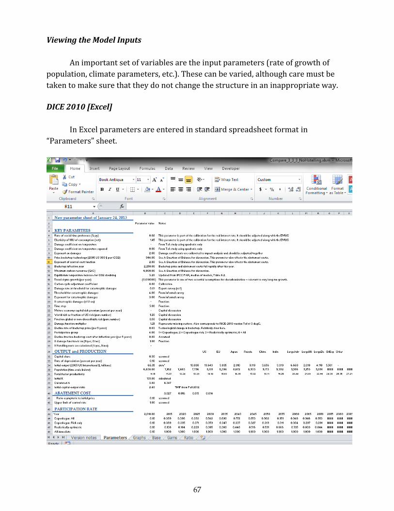
67

Viewing the Model Inputs

An important set of variables are the input parameters (rate of growth of

population, climate parameters, etc.). These can be varied, although care must be

taken to make sure that they do not change the structure in an inappropriate way.

DICE 2010 [Excel]

In Excel parameters are entered in standard spreadsheet format in

“Parameters” sheet.

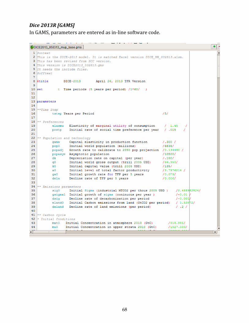
68

Dice 2013R [GAMS]

In GAMS, parameters are entered as in-line software code.

69

Viewing the Model Structure

DICE 2013R [Excel]

The model structure of DICE 2013R Excel is contained within the formulas

entered on each sheet. For example, the atmospheric concentrations of CO2 are

shown as a formula below. There are about 28,000 ‘lines of code’ (discrete cells) in

the Excel version, so the model is possibly subject to errors. Users should be very

careful when changing parameters to make sure that they have checked the results.

70

Dice 2013R [GAMS]

The GAMS code is written in a high-level language and is much more succinct.

For the base and optimal runs, it consists of about 330 lines of code (of which about

half are comments, blank, or otherwise trivial). The following shows the way the

model structure (equation set) is defined and written.

71

Definitions of variables

This section answers the questions: What does this variable mean? Where are these

terms defined?

DICE 2013R [Excel]

In Excel, the explanations are written in column A.

DICE 2013R [GAMS]

In GAMS, the definitions are given when a variable is declared:

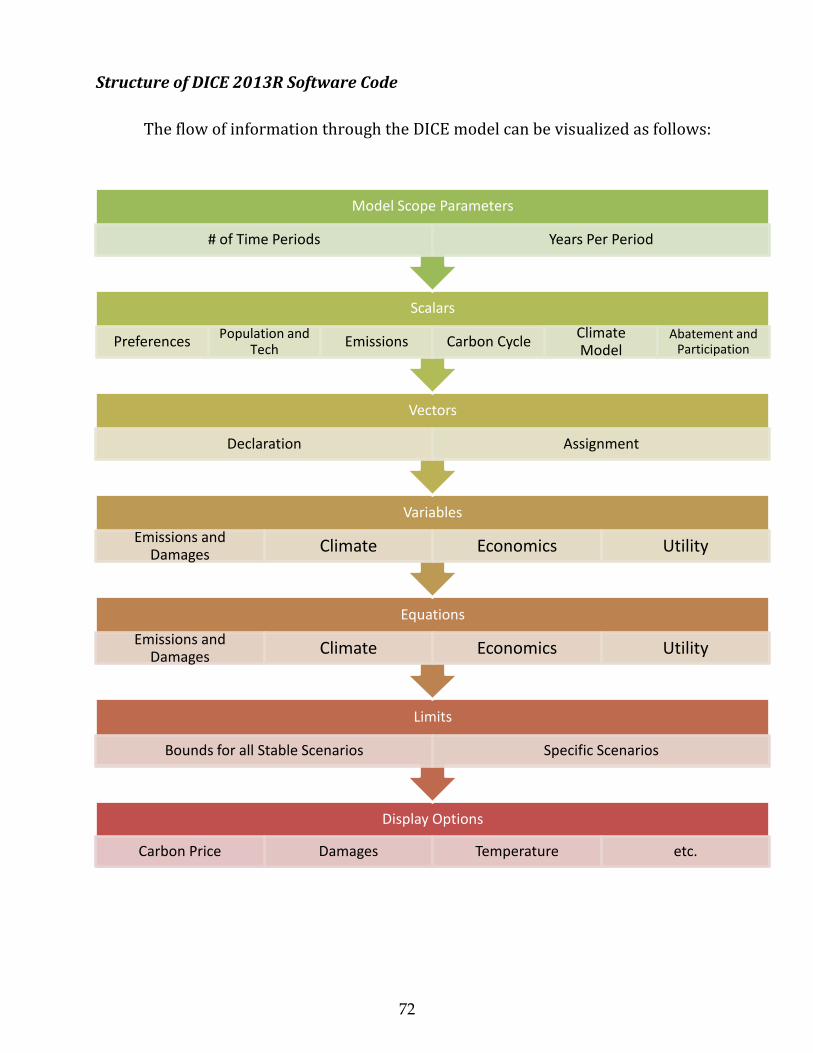
72

Structure of DICE 2013R Software Code

The flow of information through the DICE model can be visualized as follows:

Display Options

Carbon Price Damages Temperature etc.

Limits

Bounds for all Stable Scenarios Specific Scenarios

Equations

Emissions and Damages

Climate Economics Utility

Variables

Emissions and Damages

Climate Economics Utility

Vectors

Declaration Assignment

Scalars

Preferences Population and

Tech Emissions Carbon Cycle

Climate Model

Abatement and Participation

Model Scope Parameters

# of Time Periods Years Per Period

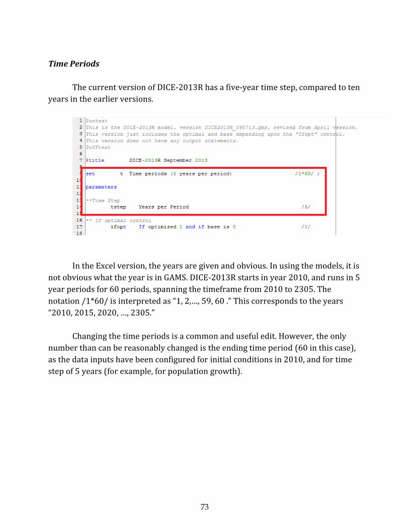
73

Time Periods

The current version of DICE-2013R has a five-year time step, compared to ten

years in the earlier versions.

In the Excel version, the years are given and obvious. In using the models, it is

not obvious what the year is in GAMS. DICE-2013R starts in year 2010, and runs in 5

year periods for 60 periods, spanning the timeframe from 2010 to 2305. The

notation /1*60/ is interpreted as “1, 2,…, 59, 60 .” This corresponds to the years

“2010, 2015, 2020, …, 2305.”

Changing the time periods is a common and useful edit. However, the only

number than can be reasonably changed is the ending time period (60 in this case),

as the data inputs have been configured for initial conditions in 2010, and for time

step of 5 years (for example, for population growth).

74

Scalars

Scalars are the easiest to change. Simply replace the number in between “/ /”

with its desired value. For example, replace “/6838/” with “/7000/” to start off the

world with a higher world population.

Vectors

Vectors are slightly more complicated to change, as they are not directly

observed until the model runs. Vectors are declared as parameters which are

indexed along a set, for example:

After being declared, they are assigned a value using simple equality statements,

typically within a loop function over the indexed set (t ‘time period’ in this example).

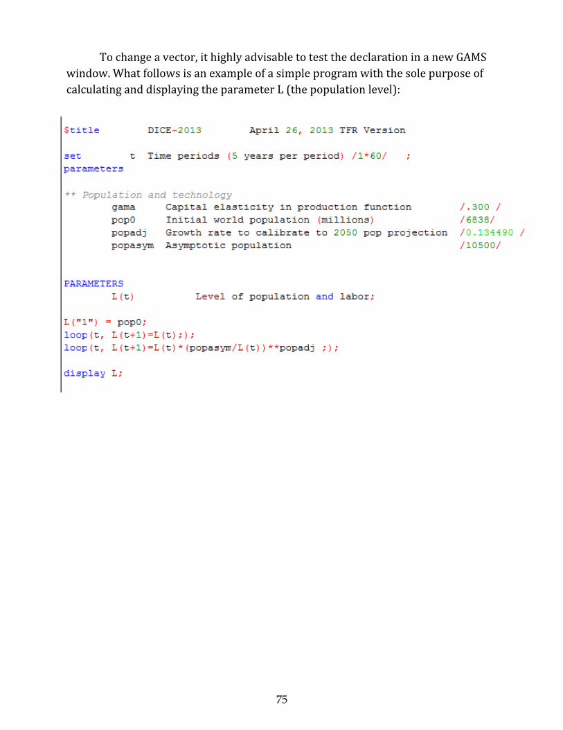
75

To change a vector, it highly advisable to test the declaration in a new GAMS

window. What follows is an example of a simple program with the sole purpose of

calculating and displaying the parameter L (the population level):

76

You might run the program and display the answer to test that the change is

correctly made, as in the following.

77

Variables and Equations

With knowledge of GAMS syntax, it is easy to edit the variables and equations.

However, editing variables/equations is by far the most perilous change because

one runs the risk of unintentionally producing a model with an entirely new

structure, or one with unstable or unrealistic solutions, or an infeasible model with

no valid solutions whatsoever.

With that caveat, here is the setup: Variables are first declared. Secondly, they

may be constrained as positive. Thirdly, the variables are used in a list of equations:

Equalities are set using “=E=” (for “equal to”); or as inequalities using “=L=” for “less

than” or =G= for “greater than”). Notably, this list of equations appears twice: There

is literally a list of equations (and their descriptions); and then a second list in which

each equation is defined mathematically.

78

Notice, again, the equations are first declared under the header “EQUATIONS”

and then secondarily defined in a lower list. For example, the EEQ or emissions

equation is declared at the top of the list above. Then the actual equation is given

directly at the bottom of the listing as “eeq(t).. E(t) =E= EIND(t) + etree(t) ;”

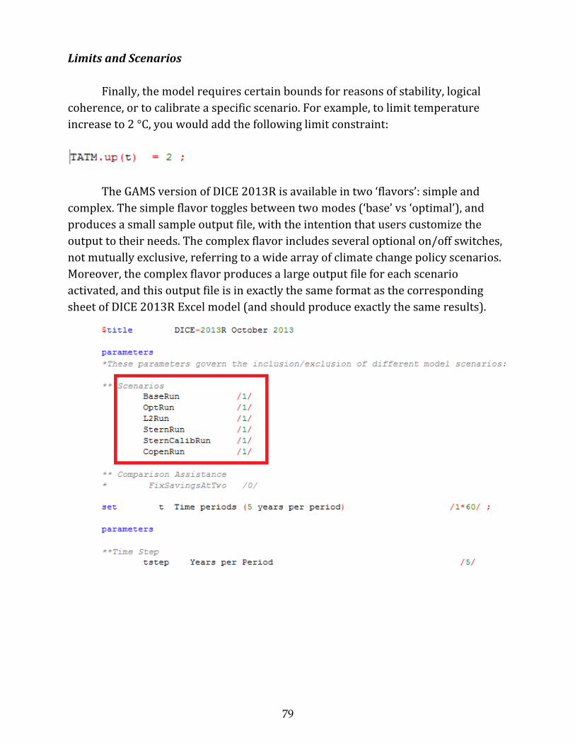
79

Limits and Scenarios

Finally, the model requires certain bounds for reasons of stability, logical

coherence, or to calibrate a specific scenario. For example, to limit temperature

increase to 2 °C, you would add the following limit constraint:

The GAMS version of DICE 2013R is available in two ‘flavors’: simple and

complex. The simple flavor toggles between two modes (‘base’ vs ‘optimal’), and

produces a small sample output file, with the intention that users customize the

output to their needs. The complex flavor includes several optional on/off switches,

not mutually exclusive, referring to a wide array of climate change policy scenarios.

Moreover, the complex flavor produces a large output file for each scenario

activated, and this output file is in exactly the same format as the corresponding

sheet of DICE 2013R Excel model (and should produce exactly the same results).

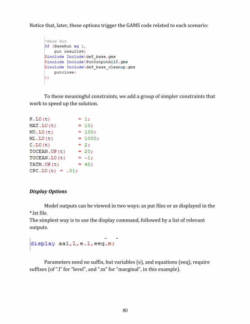
80

Notice that, later, these options trigger the GAMS code related to each scenario:

To these meaningful constraints, we add a group of simpler constraints that

work to speed up the solution.

Display Options

Model outputs can be viewed in two ways: as put files or as displayed in the

*.lst file.

The simplest way is to use the display command, followed by a list of relevant

outputs.

Parameters need no suffix, but variables (e), and equations (eeq), require

suffixes (of “.l” for “level”, and “.m” for “marginal”, in this example).

81

The above statement produces the following results in the .lst file:

“Parameter L” shows population, where “1” is 2010 is 6838 million, and so forth.

“E.L” is the emissions of CO2 in billions (G or giga) of tons of CO2. The “CPRICE.L” is

the market price of CO2 emissions in the optimized runs, also the social cost of

carbon. Note that these numbers are not necessarily correct and were created to

serve as an example.

82

Further readings

Further readings on the GAMS model can be found on the GAMS site at

http://www.gams.com/docs/document.htm.

Manuals for Solver can be found at http://www.solver.com/user-guides-

frontline-systems-excel-solvers.

One of the leading scholars who has developed GAMS for energy and

economic modeling is Tom Rutherford. See for example his “Solution Software for

Computable General Equilibrium Modeling,” with Mark Horridge, Alex Meeraus and

Ken Pearson in Handbook of Computable General Equilibrium Modeling (ISBN:

9780444595683), Peter B. Dixon and Dale W. Jorgenson (eds.), Elsevier, 1331–1381,

2013.

83

XII. Appendix B. GAMS Code for Different Vintages of the DICE

Model

This appendix contains the GAMS codes for four vintages of models: 1992-94, 1999,

2007, and 2013R. There were intermediate vintages as well, but these were the most

thoroughly documented and form the basis of most of the publications. The RICE model

program is published in Nordhaus and Boyer (2000) as well. These can be run by simply

creating a *.gms file, copying the text in, and running. There may be some formatting

problems, but these should be easily corrected.

A. 1992-1994 version of DICE model

* DICE123a

* July 28, 1994

* This is an optimal growth model to calculate the optimal control

* rate and timing for the abatement of CO2 and other Greenhouse Gases.

* This is the standard model used for Science (Nov. 1992) and for

* the base model in W. Nordhaus, Managing the Global Commons,

* MIT Press, 1994, forthcoming.

SETS T Time periods /1*40/

TFIRST(T) First period

TLAST(T) Last period

SCALARS BET Elasticity of marginal utility /0/

R Rate of social time pref per year /.03/

GL0 Growth rate of population per decade /.223/

DLAB Decline rate of pop growth per dec /.195/

DELTAM Removal rate carbon per decade /.0833/

GA0 Initial growth rate for technology per dec /.15/

DELA Decline rate of technology per dec /.11 /

SIG0 CO2-equiv-GNP ratio /.519/

GSIGMA Growth of sigma per decade /-.1168/

DK Depreciation rate on capital per year /.10/

GAMA Capital elasticity in output /.25/

M0 CO2-equiv concentrations 1965 bill t C /677/

TL0 Lower stratum temperature (C) 1965 /.10/

T0 Atmospheric temperature (C) 1965 /.2/

ATRET Marginal atmospheric retention rate /.64/

Q0 1965 world gross output trillions 89 US dol /8.519/

LL0 1965 world population millions /3369/

K0 1965 value capital billions 1989 US dollars /16.03/

C1 Coefficient for upper level /.226/

LAM Climate feedback factor /1.41/

C3 Coefficient trans upper to lower stratum /.440/

C4 Coeff of transfer for lower level /.02/

A0 Initial level of total factor productivity /.00963/

A1 Damage coeff for co2 doubling (frac GWP) /.0133/

B1 Intercept control cost function /.0686/

B2 Exponent of control cost function /2.887/

PHIK transversality coeff capital /140 /

PHIM Transversality coeff carbon ($ per ton) /-9/

84

PHITE Transversalit coeff temper (bill $ per deg C) /-7000 /

PARAMETERS L(T) Level of population and labor

AL(T) Level of Total factor productivity

SIGMA(T) Emissions-output ratio

RR(T) Discount factor

GA(T) Growth rate of T. F. P. from 0 to T

FORCOTH(T) Exogenous forcing other greenhouse gases

GL(T) Growth rate of labor 0 to T

GSIG(T) Cumulative improvement of energy efficiency

DUM(T) dummy variable 0 except 1 in last period;

TFIRST(T) = YES$(ORD(T) EQ 1);

TLAST(T) = YES$(ORD(T) EQ CARD(T));

DISPLAY TFIRST, TLAST;

GL(T) = (GL0/DLAB)*(1-exp(-DLAB*(ord(t)-1)));

L(T)=LL0*exp(GL(t));

GA(T) = (GA0/DELA)*(1-exp(-DELA*(ord(t)-1)));

AL(T) = a0*exp(GA(t));

GSIG(T) = (GSIGMA/DELA)*(1-exp(-DELA*(ord(t)-1)));

SIGMA(T)=SIG0*exp(GSIG(t));

DUM(T)=1$(ord(T) eq card(T));

RR(T) = (1+R)**(10*(1-ord(t)));

FORCOTH(T) = 1.42;

FORCOTH(T)$(ord(t) lt 15) = .2604+.125*ord(T)-.0034*ord(t)**2;

VARIABLES MIU(T) Emission control rate GHGs

FORC(T) Radiative forcing, W per m2

TE(T) Temperature, atmosphere C

TL(T) Temperature, lower ocean C

M(T) CO2-equiv concentration bill t

E(T) CO2-equiv emissions bill t

C(T) Consumption trill US dollars

K(T) Capital stock trill US dollars

CPC(T) Per capita consumption thousands US dol

PCY(t) Per capita income thousands US dol

I(T) Investment trill US dollars

S(T) Savings rate as fraction of GWP

RI(T) Interest rate per annum

TRANS(T) transversality variable last period

Y(T) OUTPUT

UTILITY;

POSITIVE VARIABLES MIU, E, TE, M, Y, C, K, I;

EQUATIONS UTIL Objective function

YY(T) Output

CC(T) Cconsumption

KK(T) Capital balance

KK0(T) Initial condition of K

KC(T) Terminal condition of K

CPCE(t) Per capita consumption

PCYE(T) Per capita income equation

EE(T) Emissions process

SEQ(T) Savings rate equation

RIEQ(T) Interest rate equation

FORCE(T) Radiative forcing equation

MM(T) CO2 distribution equation

MM0(T) Initial condition for M

85

TTE(T) Temperature-climate equation for atmosphere

TTE0(T) Initial condition for atmospheric temp

TLE(T) Temperature-climate equation for lower oceans

TRANSE(t) Transversality condition

TLE0(T) Initial condition for lower ocean;

KK(T).. K(T+1) =L= (1-DK)**10 *K(T)+10*I(T);

KK0(TFIRST).. K(TFIRST) =E= K0;

KC(TLAST).. R*K(TLAST) =L= I(TLAST);

EE(T).. E(T)=G=10*SIGMA(T)*(1-MIU(T))*AL(T)*L(T)**(1-GAMA)*K(T)**GAMA;

FORCE(T).. FORC(T) =E= 4.1*(log(M(T)/590)/log(2))+FORCOTH(T);

MM0(TFIRST).. M(TFIRST) =E= M0;

MM(T+1).. M(T+1) =E= 590+ATRET*E(T)+(1 - DELTAM)*(M(T)-590);

TTE0(TFIRST).. TE(TFIRST) =E= T0;

TTE(T+1).. TE(T+1) =E= TE(t)+C1*(FORC(t)-LAM*TE(t)-C3*(TE(t)-TL(t)));

TLE0(TFIRST).. TL(TFIRST) =E= TL0;

TLE(T+1).. TL(T+1) =E= TL(T)+C4*(TE(T)-TL(T));

YY(T).. Y(T) =E= AL(T)*L(T)**(1-GAMA)*K(T)**GAMA*(1-B1*(MIU(T)**B2))

/(1+(A1/9)*SQR(TE(T)));

SEQ(T).. S(T) =e= I(T)/(.001+Y(T));

RIEQ(T).. RI(T) =E= GAMA*Y(T)/K(T)- (1-(1-DK)**10)/10 ;

CC(T).. C(T) =E= Y(T)-I(T);

CPCE(T).. CPC(T) =e= C(T)*1000/L(T);

PCYE(T).. PCY(T) =e= Y(T)*1000/L(T);

TRANSE(TLAST).. TRANS(TLAST)=E=RR(TLAST)

*(PHIK*K(TLAST)+PHIM*M(TLAST)+PHITE*TE(TLAST));

UTIL.. UTILITY =E=

SUM(T, 10 *RR(T)*L(T)*LOG(C(T)/L(T))/.55 +TRANS(T)*DUM(T));

* Upper and Lower Bounds: General for stability

MIU.up(T) = 0.99;

MIU.lo(T) = 0.01;

K.lo(T) = 1;

TE.up(t) = 20;

M.lo(T) = 600;

C.LO(T) = 2;

* Upper and lower bounds for historical constraints

MIU.fx('1')=0.;

MIU.fx('2')=0.;

MIU.fx('3')=0.;

* Solution options

option iterlim = 99900;

option reslim = 99999;

option solprint = off;

option limrow = 0;

option limcol = 0;

model CO2 /all/;

solve CO2 maximizing UTILITY using nlp ;

display Y.l, C.l, S.l, K.l, MIU.l, E.l, M.l, TE.l, FORC.l, RI.l,

CC.m, EE.m, KK.m, MM.m, TTE.m, CPC.l, TL.l, PCY.l, i.l;

display SIGMA, RR, L, AL, DUM, FORCOTH;

86

B. 1999 version of DICE model

** DICE 1999. Optimal carbon policy

** New optimal DICE as of 5/5/99

** Calibrated to RICE99 of 5/3/99

SETS T Time periods /1*40/

TFIRST(T) First period

TLAST(T) Last period

tearly(T) First 20 periods

TLATE(T) Second 20 periods;

SCALARS

SRTP Initial rate of social time preference per year /.03/

DR Decline rate of social time preference per year /.0025719/

GL0 Growth rate of population per decade /.157/

DLAB Decline rate of pop growth per decade /.2220/

A0 Initial level of total factor productivity /.01685/

GA0 Initial growth rate for technology per decade /.038/

DELA Decline rate of technol. change per decade /.00000001/

SIG0 CO2-equivalent emissions-GNP ratio /.274/

GSIGMA Growth of sigma per decade /-.158854/

desig Decline rate of decarbonization /.02358711/

desig2 Quadratic term in decarbonization /-.00085/

DK Depreciation rate on capital per year /.10/

GAMA Capital elasticity in production function /.30/

MAT1990 Concentration in atmosphere 1990 (b.t.c.) /735/

MU1990 Concentration in upper strata 1990 (b.t.c) /781/

ML1990 Concentration in lower strata 1990 (b.t.c) /19230/

b11 Carbon cycle transition matrix /0.66616/

b12 Carbon cycle transition matrix /0.33384/

b21 Carbon cycle transition matrix /0.27607/

b22 Carbon cycle transition matrix /0.60897/

b23 Carbon cycle transition matrix /0.11496/

b32 Carbon cycle transition matrix /0.00422/

b33 Carbon cycle transition matrix /0.99578/

TL0 1985 lower strat. temp change (C) from 1900 /.06/

T0 1985 atmospheric temp change (C)from 1900 /.43/

Q0 1990 world gross output trill 90 US dollars /21.08/

LL0 1990 world population millions /5632.7/

K0 1990 value capital trill 1990 US dollars /47/

C1 Climate-equation coefficient for upper level /.226/

LAM Climate feedback factor /1.41/

C3 Transfer coeffic. upper to lower stratum /.440/

C4 Transfer coeffic for lower level /.02/

A1 Damage coeff linear term /-.0045/

A2 Damage coeff quadratic term /.0035/

COST10 Intercept control cost function /.03/

COST2 Exponent of control cost function /2.15/

ET0 C Emiss from deforest (bill tons per dec) /11.28/

dmiufunc Decline in cost of abatement function (per decade) /-.08/

decmiu Change in decline of cost function /.005/

coefopt1 Scaling coefficient in the objective function /.333187/

coefopt2 Scaling coefficient in the objective function /5135680.6/ ;

PARAMETERS

L(T) Level of population and labor

AL(T) Level of total factor productivity

SIGMA(T) CO2-equivalent-emissions output ratio

87

R(T) Instantaeous rate of social time preference

RR(T) Average utility social discount rate

GA(T) Growth rate of productivity from 0 to T

FORCOTH(T) Exogenous forcing for other greenhouse gases

GL(T) Growth rate of labor 0 to T

gcost1

GSIG(T) Cumulative improvement of energy efficiency

ETREE(T) Emissions from deforestation

cost1(t) cost function for abatement ;

TFIRST(T) = YES$(ORD(T) EQ 1);

TLAST(T) = YES$(ORD(T) EQ CARD(T));

TEARLY(T) = YES$(ORD(T) LE 20);

TLATE(T) = YES$(ORD(T) GE 21);

DISPLAY TFIRST, TLAST;

GL(T) = (GL0/DLAB)*(1-exp(-DLAB*(ord(t)-1)));

L(T)=LL0*exp(GL(t));

ga(T)=ga0*EXP(-dela*10*(ORD(T)-1));

al("1") = a0;

LOOP(T,

al(T+1)=al(T)/((1-ga(T)));

);

gsig(T)=gsigma*EXP ( -desig*10*(ORD(T)-1) - desig2*10* ((ord(t)-1)**2) ) ;

sigma("1")=sig0;

LOOP(T,

sigma(T+1)=(sigma(T)/((1-gsig(T+1))));

);

gcost1(T)=dmiufunc*EXP(-decmiu*10*(ORD(T)-1));

cost1("1")=cost10;

LOOP(T,

cost1(T+1)=cost1(T)/((1+gcost1(T+1)));

);

ETREE(T) = ET0*(1-0.1)**(ord(T)-1);

R(T)=srtp*EXP(-DR*10*(ORD(T)-1));

RR("1")=1;

LOOP(T,

RR(T+1)=RR(T)/((1+R(T))**10);

);

FORCOTH(T)=(-0.1965+.149*(ORD(T)-1)-.0019*(ORD(T)-1)**2)$

(ORD(T) LT 12) + 1.15$(ORD(T) GE 12);

VARIABLES

MIU(T) Emission control rate GHGs

FORC(T) Radiative forcing, W per m2

TE(T) Temperature, atmosphere C

TL(T) Temperature, lower ocean C

MAT(T) Carbon concentration in atmosphere (b.t.c.)

MU(T) Carbon concentration in shallow oceans (b.t.c.)

ML(T) Carbon concentration in lower oceans (b.t.c.)

E(T) CO2-equivalent emissions bill t

C(T) Consumption trill US dollars

K(T) Capital stock trill US dollars

CPC(T) Per capita consumption thousands US dol

PCY(t) Per capita income thousands US dol

I(T) Investment trill US dollars

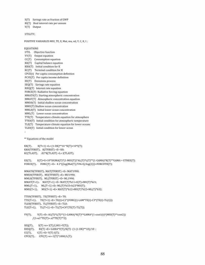
88

S(T) Savings rate as fraction of GWP

RI(T) Real interest rate per annum

Y(T) Output

UTILITY;

POSITIVE VARIABLES MIU, TE, E, Mat, mu, ml, Y, C, K, I ;

EQUATIONS

UTIL Objective function

YY(T) Output equation

CC(T) Consumption equation

KK(T) Capital balance equation

KK0(T) Initial condition for K

KC(T) Terminal condition for K

CPCE(t) Per capita consumption definition

PCYE(T) Per capita income definition

EE(T) Emissions process

SEQ(T) Savings rate equation

RIEQ(T) Interest rate equation

FORCE(T) Radiative forcing equation

MMAT0(T) Starting atmospheric concentration

MMAT(T) Atmospheric concentration equation

MMU0(T) Initial shallow ocean concentration

MMU(T) Shallow ocean concentration

MML0(T) Initial lower ocean concentration

MML(T) Lower ocean concentration

TTE(T) Temperature-climate equation for atmosphere

TTE0(T) Initial condition for atmospheric temperature

TLE(T) Temperature-climate equation for lower oceans

TLE0(T) Initial condition for lower ocean

;

** Equations of the model

KK(T).. K(T+1) =L= (1-DK)**10 *K(T)+10*I(T);

KK0(TFIRST).. K(TFIRST) =E= K0;

KC(TLAST).. .02*K(TLAST) =L= I(TLAST);

EE(T).. E(T)=G=10*SIGMA(T)*(1-MIU(T))*AL(T)*L(T)**(1-GAMA)*K(T)**GAMA + ETREE(T);

FORCE(T).. FORC(T) =E= 4.1*((log(Mat(T)/596.4)/log(2)))+FORCOTH(T);

MMAT0(TFIRST).. MAT(TFIRST) =E= MAT1990;

MMU0(TFIRST).. MU(TFIRST) =E= MU1990;

MML0(TFIRST).. ML(TFIRST) =E= ML1990;

MMAT(T+1).. MAT(T+1) =E= MAT(T)*b11+E(T)+MU(T)*b21;

MML(T+1).. ML(T+1) =E= ML(T)*b33+b23*MU(T);

MMU(T+1).. MU(T+1) =E= MAT(T)*b12+MU(T)*b22+ML(T)*b32;

TTE0(TFIRST).. TE(TFIRST) =E= T0;

TTE(T+1).. TE(T+1) =E= TE(t)+C1*(FORC(t)-LAM*TE(t)-C3*(TE(t)-TL(t)));

TLE0(TFIRST).. TL(TFIRST) =E= TL0;

TLE(T+1).. TL(T+1) =E= TL(T)+C4*(TE(T)-TL(T));

YY(T).. Y(T) =E= AL(T)*L(T)**(1-GAMA)*K(T)**GAMA*(1-cost1(t)*(MIU(T)**cost2))

/(1+a1*TE(T)+ a2*TE(T)**2);

SEQ(T).. S(T) =e= I(T)/(.001+Y(T));

RIEQ(T).. RI(T) =E= GAMA*Y(T)/K(T)- (1-(1-DK)**10)/10 ;

CC(T).. C(T) =E= Y(T)-I(T);

CPCE(T).. CPC(T) =e= C(T)*1000/L(T);

89

PCYE(T).. PCY(T) =e= Y(T)*1000/L(T);

UTIL.. UTILITY =E= SUM(T, 10 *RR(T)*L(T)*LOG(C(T)/L(T))/coefopt1)+ coefopt2 ;

** Upper and Lower Bounds: General conditions imposed for stability

MIU.up(T) = 1.0;

MIU.lo(T) = 0.000001;

K.lo(T) = 1;

TE.up(t) = 12;

MAT.lo(T) = 10;

MU.lo(t) = 100;

ML.lo(t) = 1000;

C.lo(T) = 2;

** Emissions control policy. Current setting is for optimal policy.

** Reinstate equation "Miu.fx(t) = .0" for no-control run.

* For base, remove the * from the following to get zero controls

*MIU.fx(t)=.0;

** Solution options

option iterlim = 99900;

option reslim = 99999;

option solprint = on;

option limrow = 0;

option limcol = 0;

model CO2 /all/;

solve CO2 maximizing UTILITY using nlp ;

solve CO2 maximizing UTILITY using nlp ;

solve CO2 maximizing UTILITY using nlp ;

** Display of results

display y.l, c.l, s.l, k.l, miu.l, e.l, te.l, forc.l, ri.l;

display cc.m, ee.m, kk.m, tte.m, cpc.l, tl.l, pcy.l, i.l;

display sigma, rr, l, al, forcoth, etree;

display mat.l,mu.l,ml.l;

Parameters

Year(t) Date

Indem(t) Industrial emissions (b.t.c. per year)

Wem(t) Total emissions (b.t.c. per year);

Year(t) = 1995 +10*(ord(t)-1);

Indem(t) = e.l(t)-etree(t);

Wem(t) = e.l(t);Parameters

Tax(t) Carbon tax ($ per ton)

damtax(t) Concentration tax ($ per ton)

dam(t) Damages

cost(t) Abatement costs;

tax(t) = -1*ee.m(t)*1000/(kk.m(t));

damtax(t) = -1*mmat.m(t)*1000/kk.m(t);

dam(t) = y.l(t)*(1-1/(1+a1*te.l(t)+ a2*te.l(t)**2));

cost(t) = y.l(t)*(cost1(t)*(miu.l(t)**cost2));

display gsig, sigma;

display ga, al, cost1, gcost1, tax,miu.l,e.l,te.l;

90

C. 2008 version of DICE model

$ontext

DICE delta version 8

July 17, 2008.

This version is used for the DICE book, A Question of Balance (YUP, 2008).

We have included only the base, Hotelling, and optimal runs.

Exclude statements are removed so that it can run as a self-contained program.

$offtext

SETS T Time periods /1*60/ ;

SCALARS

** Preferences

B_ELASMU Elasticity of marginal utility of consumption / 2.0 /

B_PRSTP Initial rate of social time preference per year / .015 /

** Population and technology

POP0 2005 world population millions /6514 /

GPOP0 Growth rate of population per decade /.35 /

POPASYM Asymptotic population / 8600 /

A0 Initial level of total factor productivity /.02722 /

GA0 Initial growth rate for technology per decade /.092 /

DELA Decline rate of technol change per decade /.001 /

DK Depreciation rate on capital per year /.100 /

GAMA Capital elasticity in production function /.300 /

Q0 2005 world gross output trill 2005 US dollars /61.1 /

K0 2005 value capital trill 2005 US dollars /137. /

** Emissions

SIG0 CO2-equivalent emissions-GNP ratio 2005 /.13418 /

GSIGMA Initial growth of sigma per decade /-.0730 /

DSIG Decline rate of decarbonization per decade /.003 /

DSIG2 Quadratic term in decarbonization / .000 /

ELAND0 Carbon emissions from land 2005(GtC per decade) / 11.000 /

** Carbon cycle

MAT2000 Concentration in atmosphere 2005 (GtC) /808.9 /

MU2000 Concentration in upper strata 2005 (GtC) /1255 /

ML2000 Concentration in lower strata 2005 (GtC) /18365 /

b11 Carbon cycle transition matrix /0.810712 /

b12 Carbon cycle transition matrix /0.189288 /

b21 Carbon cycle transition matrix /0.097213 /

b22 Carbon cycle transition matrix /0.852787 /

b23 Carbon cycle transition matrix /0.05 /

b32 Carbon cycle transition matrix /0.003119 /

b33 Carbon cycle transition matrix /0.996881 /

** Climate model

T2XCO2 Equilibrium temp impact of CO2 doubling oC / 3 /

FEX0 Estimate of 2000 forcings of non-CO2 GHG / -.06 /

FEX1 Estimate of 2100 forcings of non-CO2 GHG / 0.30 /

TOCEAN0 2000 lower strat. temp change (C) from 1900 /.0068 /

TATM0 2000 atmospheric temp change (C)from 1900 /.7307 /

C1 Climate-equation coefficient for upper level /.220 /

C3 Transfer coeffic upper to lower stratum /.300 /

C4 Transfer coeffic for lower level /.050 /

FCO22X Estimated forcings of equilibrium co2 doubling /3.8 /

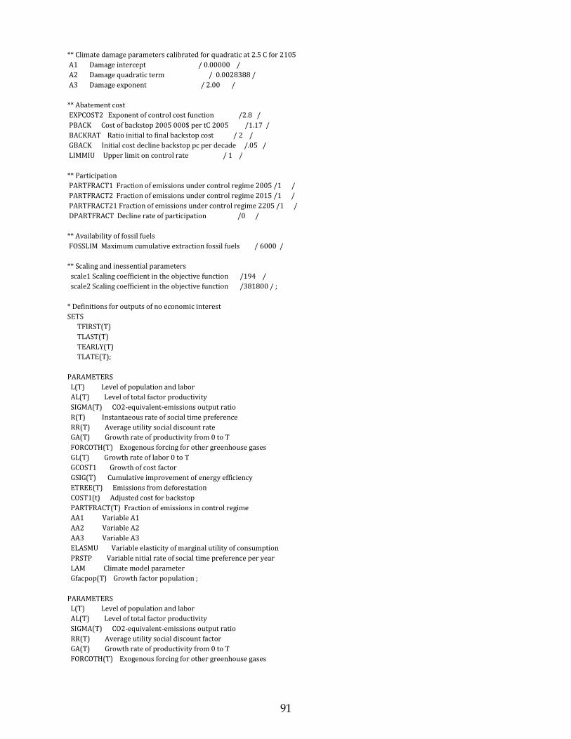
91

** Climate damage parameters calibrated for quadratic at 2.5 C for 2105

A1 Damage intercept / 0.00000 /

A2 Damage quadratic term / 0.0028388 /

A3 Damage exponent / 2.00 /

** Abatement cost

EXPCOST2 Exponent of control cost function /2.8 /

PBACK Cost of backstop 2005 000$ per tC 2005 /1.17 /

BACKRAT Ratio initial to final backstop cost / 2 /

GBACK Initial cost decline backstop pc per decade /.05 /

LIMMIU Upper limit on control rate / 1 /

** Participation

PARTFRACT1 Fraction of emissions under control regime 2005 /1 /

PARTFRACT2 Fraction of emissions under control regime 2015 /1 /

PARTFRACT21 Fraction of emissions under control regime 2205 /1 /

DPARTFRACT Decline rate of participation /0 /

** Availability of fossil fuels

FOSSLIM Maximum cumulative extraction fossil fuels / 6000 /

** Scaling and inessential parameters

scale1 Scaling coefficient in the objective function /194 /

scale2 Scaling coefficient in the objective function /381800 / ;

* Definitions for outputs of no economic interest

SETS

TFIRST(T)

TLAST(T)

TEARLY(T)

TLATE(T);

PARAMETERS

L(T) Level of population and labor

AL(T) Level of total factor productivity

SIGMA(T) CO2-equivalent-emissions output ratio

R(T) Instantaeous rate of social time preference

RR(T) Average utility social discount rate

GA(T) Growth rate of productivity from 0 to T

FORCOTH(T) Exogenous forcing for other greenhouse gases

GL(T) Growth rate of labor 0 to T

GCOST1 Growth of cost factor

GSIG(T) Cumulative improvement of energy efficiency

ETREE(T) Emissions from deforestation

COST1(t) Adjusted cost for backstop

PARTFRACT(T) Fraction of emissions in control regime

AA1 Variable A1

AA2 Variable A2

AA3 Variable A3

ELASMU Variable elasticity of marginal utility of consumption

PRSTP Variable nitial rate of social time preference per year

LAM Climate model parameter

Gfacpop(T) Growth factor population ;

PARAMETERS

L(T) Level of population and labor

AL(T) Level of total factor productivity

SIGMA(T) CO2-equivalent-emissions output ratio

RR(T) Average utility social discount factor

GA(T) Growth rate of productivity from 0 to T

FORCOTH(T) Exogenous forcing for other greenhouse gases

92

GL(T) Growth rate of labor 0 to T

GCOST1 Growth of cost factor

GSIG(T) Cumulative improvement of energy efficiency

ETREE(T) Emissions from deforestation

COST1(t) Adjusted cost for backstop

PARTFRACT(T) Fraction of emissions in control regime

AA1 Variable A1

AA2 Variable A2

AA3 Variable A3

ELASMU Variable elasticity of marginal utility of consumption

PRSTP Variable nitial rate of social time preference per year

LAM Climate model parameter

Gfacpop(T) Growth factor population ;

* Unimportant definitions to reset runs

TFIRST(T) = YES$(ORD(T) EQ 1);

TLAST(T) = YES$(ORD(T) EQ CARD(T));

TEARLY(T) = YES$(ORD(T) LE 20);

TLATE(T) = YES$(ORD(T) GE 21);

AA1 = A1;

AA2 = A2;

AA3 = A3;

ELASMU = B_ELASMU;

PRSTP = B_PRSTP;

b11 = 1 - b12;

b21 = 587.473*B12/1143.894;

b22 = 1 - b21 - b23;

b32 = 1143.894*b23/18340;

b33 = 1 - b32 ;

* Important parameters for the model

LAM = FCO22X/ T2XCO2;

Gfacpop(T) = (exp(gpop0*(ORD(T)-1))-1)/exp(gpop0*(ORD(T)-1));

L(T)=POP0* (1- Gfacpop(T))+Gfacpop(T)*popasym;

ga(T)=ga0*EXP(-dela*10*(ORD(T)-1));

al("1") = a0;

LOOP(T, al(T+1)=al(T)/((1-ga(T))););

gsig(T)=gsigma*EXP(-dsig*10*(ORD(T)-1)-dsig2*10*((ord(t)-1)**2));sigma("1")=sig0;LOOP(T,sigma(T+1)=(sigma(T)/((1-

gsig(T+1)))););

cost1(T) = (PBACK*SIGMA(T)/EXPCOST2)* ( (BACKRAT-1+ EXP (-gback* (ORD(T)-1) ) )/BACKRAT);

ETREE(T) = ELAND0*(1-0.1)**(ord(T)-1);

RR(t)=1/((1+prstp)**(10*(ord(T)-1)));

FORCOTH(T)= FEX0+ .1*(FEX1-FEX0)*(ORD(T)-1)$(ORD(T) LT 12)+ 0.36$(ORD(T) GE 12);

partfract(t) = partfract21;

PARTFRACT(T)$(ord(T)<25) = Partfract21 + (PARTFRACT2-Partfract21)*exp(-DPARTFRACT*(ORD(T)-2));

partfract("1")= PARTFRACT1;

VARIABLES

MIU(T) Emission control rate GHGs

FORC(T) Radiative forcing in watts per m2

TATM(T) Temperature of atmosphere in degrees C

TOCEAN(T) Temperatureof lower oceans degrees C

MAT(T) Carbon concentration in atmosphere GtC

MATAV(T) Average concentrations

MU(T) Carbon concentration in shallow oceans Gtc

ML(T) Carbon concentration in lower oceans GtC

E(T) CO2-equivalent emissions GtC

C(T) Consumption trillions US dollars

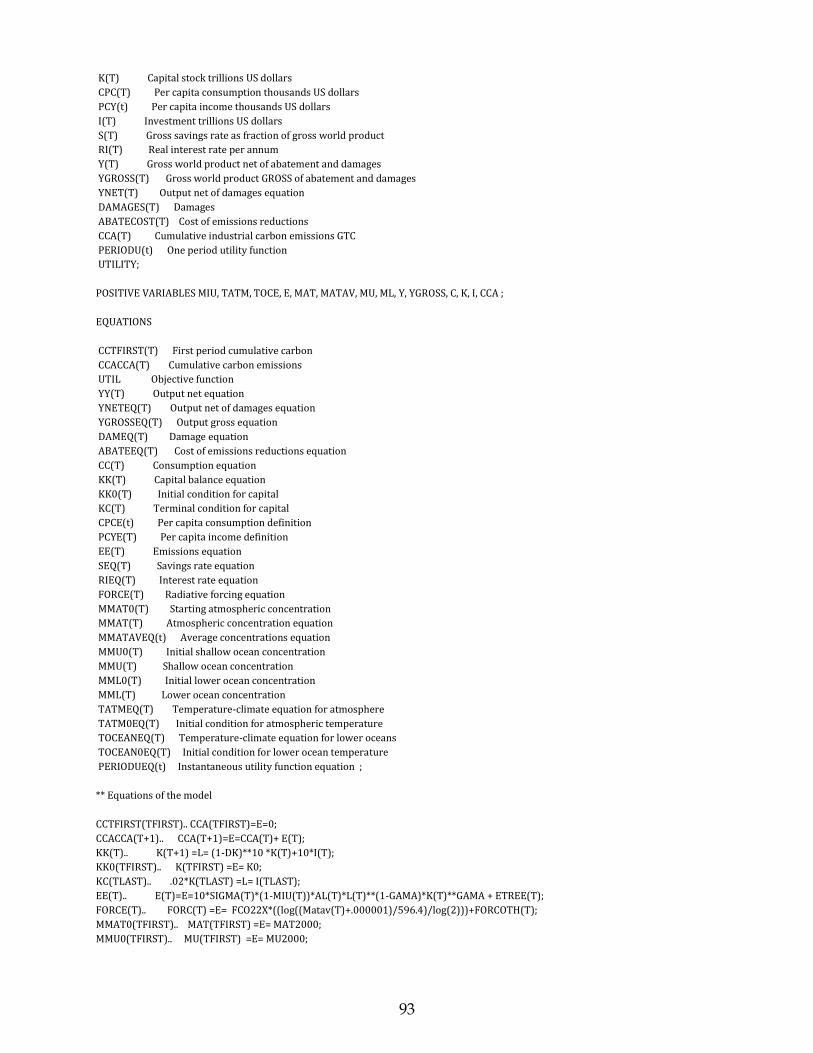
93

K(T) Capital stock trillions US dollars

CPC(T) Per capita consumption thousands US dollars

PCY(t) Per capita income thousands US dollars

I(T) Investment trillions US dollars

S(T) Gross savings rate as fraction of gross world product

RI(T) Real interest rate per annum

Y(T) Gross world product net of abatement and damages

YGROSS(T) Gross world product GROSS of abatement and damages

YNET(T) Output net of damages equation

DAMAGES(T) Damages

ABATECOST(T) Cost of emissions reductions

CCA(T) Cumulative industrial carbon emissions GTC

PERIODU(t) One period utility function

UTILITY;

POSITIVE VARIABLES MIU, TATM, TOCE, E, MAT, MATAV, MU, ML, Y, YGROSS, C, K, I, CCA ;

EQUATIONS

CCTFIRST(T) First period cumulative carbon

CCACCA(T) Cumulative carbon emissions

UTIL Objective function

YY(T) Output net equation

YNETEQ(T) Output net of damages equation

YGROSSEQ(T) Output gross equation

DAMEQ(T) Damage equation

ABATEEQ(T) Cost of emissions reductions equation

CC(T) Consumption equation

KK(T) Capital balance equation

KK0(T) Initial condition for capital

KC(T) Terminal condition for capital

CPCE(t) Per capita consumption definition

PCYE(T) Per capita income definition

EE(T) Emissions equation

SEQ(T) Savings rate equation

RIEQ(T) Interest rate equation

FORCE(T) Radiative forcing equation

MMAT0(T) Starting atmospheric concentration

MMAT(T) Atmospheric concentration equation

MMATAVEQ(t) Average concentrations equation

MMU0(T) Initial shallow ocean concentration

MMU(T) Shallow ocean concentration

MML0(T) Initial lower ocean concentration

MML(T) Lower ocean concentration

TATMEQ(T) Temperature-climate equation for atmosphere

TATM0EQ(T) Initial condition for atmospheric temperature

TOCEANEQ(T) Temperature-climate equation for lower oceans

TOCEAN0EQ(T) Initial condition for lower ocean temperature

PERIODUEQ(t) Instantaneous utility function equation ;

** Equations of the model

CCTFIRST(TFIRST).. CCA(TFIRST)=E=0;

CCACCA(T+1).. CCA(T+1)=E=CCA(T)+ E(T);

KK(T).. K(T+1) =L= (1-DK)**10 *K(T)+10*I(T);

KK0(TFIRST).. K(TFIRST) =E= K0;

KC(TLAST).. .02*K(TLAST) =L= I(TLAST);

EE(T).. E(T)=E=10*SIGMA(T)*(1-MIU(T))*AL(T)*L(T)**(1-GAMA)*K(T)**GAMA + ETREE(T);

FORCE(T).. FORC(T) =E= FCO22X*((log((Matav(T)+.000001)/596.4)/log(2)))+FORCOTH(T);

MMAT0(TFIRST).. MAT(TFIRST) =E= MAT2000;

MMU0(TFIRST).. MU(TFIRST) =E= MU2000;

94

MML0(TFIRST).. ML(TFIRST) =E= ML2000;

MMAT(T+1).. MAT(T+1) =E= MAT(T)*b11+MU(T)*b21 + E(T);

MMATAVEQ(t).. MATAV(T) =e= (MAT(T)+MAT(T+1))/2 ;

MML(T+1).. ML(T+1) =E= ML(T)*b33+b23*MU(T);

MMU(T+1).. MU(T+1) =E= MAT(T)*b12+MU(T)*b22+ML(T)*b32;

TATM0EQ(TFIRST).. TATM(TFIRST) =E= TATM0;

TATMEQ(T+1).. TATM(T+1) =E= TATM(t)+C1*(FORC(t+1)-LAM*TATM(t)-C3*(TATM(t)-TOCEAN(t)));

TOCEAN0EQ(TFIRST).. TOCEAN(TFIRST) =E= TOCEAN0;

TOCEANEQ(T+1).. TOCEAN(T+1) =E= TOCEAN(T)+C4*(TATM(T)-TOCEAN(T));

YGROSSEQ(T).. YGROSS(T) =e= AL(T)*L(T)**(1-GAMA)*K(T)**GAMA;

DAMEQ(T).. DAMAGES(t) =E= YGROSS(T)- YGROSS(T)/(1+aa1*TATM(T)+ aa2*TATM(T)**aa3);

YNETEQ(T).. YNET(T) =E= YGROSS(T)/(1+aa1*TATM(T)+ aa2*TATM(T)**aa3);

ABATEEQ(T).. ABATECOST(T) =E= (PARTFRACT(T)**(1-expcost2))*YGROSS(T)*(cost1(t)*(MIU(T)**EXPcost2));

YY(T).. Y(T) =E= YGROSS(T)*((1-(PARTFRACT(T)**(1-expcost2))*cost1(t)*(MIU(T)**EXPcost2)))/(1+aa1*TATM(T)+

aa2*TATM(T)**aa3);

SEQ(T).. S(T) =E= I(T)/(.001+Y(T));

RIEQ(T).. RI(T) =E= GAMA*Y(T)/K(T)- (1-(1-DK)**10)/10 ;

CC(T).. C(T) =E= Y(T)-I(T);

CPCE(T).. CPC(T) =E= C(T)*1000/L(T);

PCYE(T).. PCY(T) =E= Y(T)*1000/L(T);

PERIODUEQ(T).. PERIODU(T) =E= ((C(T)/L(T))**(1-ELASMU)-1)/(1-ELASMU);

UTIL.. UTILITY =E= SUM(T, 10 *RR(T)*L(T)*(PERIODU(T))/scale1)+ scale2 ;

** Upper and Lower Bounds: General conditions for stability

K.lo(T) = 100;

MAT.lo(T) = 10;

MU.lo(t) = 100;

ML.lo(t) = 1000;

C.lo(T) = 20;

TOCEAN.up(T) = 20;

TOCEAN.lo(T) = -1;

TATM.up(t) = 20;

miu.up(t) = LIMMIU;

partfract("1")= 0.25372;

* First period predetermined by Kyoto Protocol

miu.fx("1") = 0.005;

** Fix savings assumption for standardization if needed

*s.fx(t)=.22;

** Cumulative limits on carbon use at 6000 GtC

CCA.up(T) = FOSSLIM;

** Solution options

option iterlim = 99900;

option reslim = 99999;

option solprint = on;

option limrow = 0;

option limcol = 0;

model CO2 /all/;

* Optimal run

* Solution for optimal run

solve CO2 maximizing UTILITY using nlp ;

solve CO2 maximizing UTILITY using nlp ;

solve CO2 maximizing UTILITY using nlp ;

solve CO2 maximizing UTILITY using nlp ;

solve CO2 maximizing UTILITY using nlp ;

95

solve CO2 maximizing UTILITY using nlp ;

* Definition of opt results

Parameters

Year(t) Date

opt_y(t)

opt_cpc(t)

opt_s(t)

opt_indem(t)

opt_sigma(t)

opt_tatm(t)

opt_mat(t)

opt_tax(t)

opt_ri(t)

opt_rr(t)

opt_al(t)

opt_forcoth(t)

opt_l(t)

opt_etree(t)

opt_yy(t)

opt_cc(t)

opt_miu(t)

opt_wem(t)

opt_ri(t)

opt_dam(t)

opt_abate(t)

opt_mcemis(t)

opt_utility

opt_scc(t) ;

Year(t) = 2005 +10*(ord(t)-1);

opt_y(t)=y.l(t);

opt_cpc(t)=cpc.l(t);

opt_s(t)=s.l(t) ;

opt_indem(t)= e.l(t)-etree(t);;

opt_sigma(t)=sigma(t) ;

opt_tatm(t)=tatm.l(t) ;

opt_mat(t)=mat.l(t) ;

opt_tax(t)=-1*ee.m(t)*1000/(kk.m(t)+.00000000001) ;

opt_ri(t)=ri.l(t);

opt_rr(t)=rr(t) ;

opt_al(t)=al(t) ;

opt_forcoth(t)=forcoth(t);

opt_l(t)=l(t);

opt_etree(t)=etree(t);

opt_yy(t)=yy.m(t) ;

opt_cc(t)=cc.m(t) ;

opt_miu(t)=miu.l(t) ;

opt_wem(t)= e.l(t);

opt_ri(t)=ri.l(t) ;

opt_dam(t)= damages.l(t);

opt_abate(t) = abatecost.l(t);

opt_mcemis(t)= expcost2*cost1(t)*miu.l(t)**(expcost2-1)/sigma(t)*1000;

opt_utility=utility.l ;

opt_scc(t)=-ee.m(t)/cc.m(t)*(1000) ;

option decimals=6;

display opt_scc,y.l,opt_miu,ee.m, cc.m, yy.m;

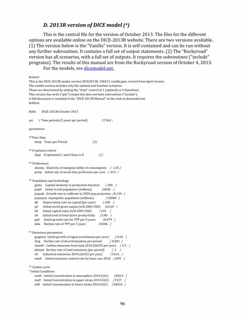
96

D. 2013R version of DICE model (*)

This is the central file for the version of October 2013. The files for the different options are available online on the DICE-2013R website. There are two versions available. (1) The version below is the “Vanilla” version. It is self-contained and can be run without any further subroutines. It contains a full set of output statements. (2) The “Rockyroad” version has all scenarios, with a full set of outputs. It requires the subroutines (“include” programs). The results of this manual are from the Rockyroad version of October 4, 2013.

For the models, see dicemodel.net.

$ontext

This is the DICE-2013R model, version DICE2013R_100413_vanilla.gms, revised from April version.

The vanilla version includes only the optimal and baseline scenarios.

These are determined by setting the "ifopt" control at 1 (optimal) or 0 (baseline).

This version has write ("put") output but does not have subroutines ("include").

A full discussion is included in the "DICE 2013R Manual" on the web at dicemodel.net.

$offtext

$title DICE-2013R October 2013

set t Time periods (5 years per period) /1*60/ ;

parameters

**Time Step

tstep Years per Period /5/

** If optimal control

ifopt If optimized 1 and if base is 0 /1/

** Preferences

elasmu Elasticity of marginal utility of consumption / 1.45 /

prstp Initial rate of social time preference per year / .015 /

** Population and technology

gama Capital elasticity in production function /.300 /

pop0 Initial world population (millions) /6838 /

popadj Growth rate to calibrate to 2050 pop projection /0.134 /

popasym Asymptotic population (millions) /10500 /

dk Depreciation rate on capital (per year) /.100 /

q0 Initial world gross output (trill 2005 USD) /63.69 /

k0 Initial capital value (trill 2005 USD) /135 /

a0 Initial level of total factor productivity /3.80 /

ga0 Initial growth rate for TFP per 5 years /0.079 /

dela Decline rate of TFP per 5 years /0.006 /

** Emissions parameters

gsigma1 Initial growth of sigma (continuous per year) /-0.01 /

dsig Decline rate of decarbonization per period /-0.001 /

eland0 Carbon emissions from land 2010 (GtCO2 per year) / 3.3 /

deland Decline rate of land emissions (per period) / .2 /

e0 Industrial emissions 2010 (GtCO2 per year) /33.61 /

miu0 Initial emissions control rate for base case 2010 /.039 /

** Carbon cycle

* Initial Conditions

mat0 Initial Concentration in atmosphere 2010 (GtC) /830.4 /

mu0 Initial Concentration in upper strata 2010 (GtC) /1527. /

ml0 Initial Concentration in lower strata 2010 (GtC) /10010. /

97

mateq Equilibrium concentration atmosphere (GtC) /588 /

mueq Equilibrium concentration in upper strata (GtC) /1350 /

mleq Equilibrium concentration in lower strata (GtC) /10000 /

* Flow paramaters

b12 Carbon cycle transition matrix /.088/

b23 Carbon cycle transition matrix /0.00250/

* These are for declaration and are defined later

b11 Carbon cycle transition matrix

b21 Carbon cycle transition matrix

b22 Carbon cycle transition matrix

b32 Carbon cycle transition matrix

b33 Carbon cycle transition matrix

sig0 Carbon intensity 2010 (kgCO2 per output 2005 USD 2010)

** Climate model parameters

t2xco2 Equilibrium temp impact (oC per doubling CO2) / 2.9 /

fex0 2010 forcings of non-CO2 GHG (Wm-2) / 0.25 /

fex1 2100 forcings of non-CO2 GHG (Wm-2) / 0.70 /

tocean0 Initial lower stratum temp change (C from 1900) /.0068 /

tatm0 Initial atmospheric temp change (C from 1900) /0.80 /

c1 Climate equation coefficient for upper level /0.098 /

c3 Transfer coefficient upper to lower stratum /0.088 /

c4 Transfer coefficient for lower level /0.025 /

fco22x Forcings of equilibrium CO2 doubling (Wm-2) /3.8 /

** Climate damage parameters

a1 Damage intercept /0 /

a2 Damage quadratic term /0.00267 /

a3 Damage exponent /2.00 /

** Abatement cost

expcost2 Exponent of control cost function / 2.8 /

pback Cost of backstop 2005$ per tCO2 2010 / 344 /

gback Initial cost decline backstop cost per period / .025 /

limmiu Upper limit on control rate after 2150 / 1.2 /

tnopol Period before which no emissions controls base / 45 /

cprice0 Initial base carbon price (2005$ per tCO2) / 1.0 /

gcprice Growth rate of base carbon price per year /.02 /

** Participation parameters

periodfullpart Period at which have full participation /21 /

partfract2010 Fraction of emissions under control in 2010 / 1 /

partfractfull Fraction of emissions under control at full time / 1 /

** Availability of fossil fuels

fosslim Maximum cumulative extraction fossil fuels (GtC) /6000/

** Scaling and inessential parameters

* Note that these are unnecessary for the calculations but are for convenience

scale1 Multiplicative scaling coefficient /0.016408662 /

scale2 Additive scaling coefficient /-3855.106895/ ;

* Program control variables

sets tfirst(t), tlast(t), tearly(t), tlate(t);

PARAMETERS

L(t) Level of population and labor

al(t) Level of total factor productivity

sigma(t) CO2-equivalent-emissions output ratio

98

rr(t) Average utility social discount rate

ga(t) Growth rate of productivity from

forcoth(t) Exogenous forcing for other greenhouse gases

gl(t) Growth rate of labor

gcost1 Growth of cost factor

gsig(t) Change in sigma (cumulative improvement of energy efficiency)

etree(t) Emissions from deforestation

cost1(t) Adjusted cost for backstop

partfract(t) Fraction of emissions in control regime

lam Climate model parameter

gfacpop(t) Growth factor population

pbacktime(t) Backstop price

optlrsav Optimal long-run savings rate used for transversality

scc(t) Social cost of carbon

cpricebase(t) Carbon price in base case ;

* Program control definitions

tfirst(t) = yes$(t.val eq 1);

tlast(t) = yes$(t.val eq card(t));

* Parameters for long-run consistency of carbon cycle

b11 = 1 - b12;

b21 = b12*MATEQ/MUEQ;

b22 = 1 - b21 - b23;

b32 = b23*mueq/mleq;

b33 = 1 - b32 ;

* Further definitions of parameters

sig0 = e0/(q0*(1-miu0));

lam = fco22x/ t2xco2;

L("1") = pop0;

loop(t, L(t+1)=L(t););

loop(t, L(t+1)=L(t)*(popasym/L(t))**popadj ;);

ga(t)=ga0*exp(-dela*5*((t.val-1)));

al("1") = a0; loop(t, al(t+1)=al(t)/((1-ga(t))););

gsig("1")=gsigma1; loop(t,gsig(t+1)=gsig(t)*((1+dsig)**tstep) ;);

sigma("1")=sig0; loop(t,sigma(t+1)=(sigma(t)*exp(gsig(t)*tstep)););

pbacktime(t)=pback*(1-gback)**(t.val-1);

cost1(t) = pbacktime(t)*sigma(t)/expcost2/1000;

etree(t) = eland0*(1-deland)**(t.val-1);

rr(t) = 1/((1+prstp)**(tstep*(t.val-1)));

forcoth(t) = fex0+ (1/18)*(fex1-fex0)*(t.val-1)$(t.val lt 19)+ (fex1-fex0)$(t.val ge 19);

optlrsav = (dk + .004)/(dk + .004*elasmu + prstp)*gama;

partfract(t)$(ord(T)>periodfullpart) = partfractfull;

partfract(t)$(ord(T)<periodfullpart+1) = partfract2010+(partfractfull-partfract2010)*(ord(t)-1)/periodfullpart;

partfract("1")= partfract2010;

cpricebase(t)= cprice0*(1+gcprice)**(5*(t.val-1));

VARIABLES

MIU(t) Emission control rate GHGs

FORC(t) Increase in radiative forcing (watts per m2 from 1900)

TATM(t) Increase temperature of atmosphere (degrees C from 1900)

TOCEAN(t) Increase temperatureof lower oceans (degrees C from 1900)

99

MAT(t) Carbon concentration increase in atmosphere (GtC from 1750)

MU(t) Carbon concentration increase in shallow oceans (GtC from 1750)

ML(t) Carbon concentration increase in lower oceans (GtC from 1750)

E(t) Total CO2 emissions (GtCO2 per year)

EIND(t) Industrial emissions (GtCO2 per year)

C(t) Consumption (trillions 2005 US dollars per year)

K(t) Capital stock (trillions 2005 US dollars)

CPC(t) Per capita consumption (thousands 2005 USD per year)

I(t) Investment (trillions 2005 USD per year)

S(t) Gross savings rate as fraction of gross world product

RI(t) Real interest rate (per annum)

Y(t) Gross world product net of abatement and damages (trillions 2005 USD per year)

YGROSS(t) Gross world product GROSS of abatement and damages (trillions 2005 USD per year)

YNET(t) Output net of damages equation (trillions 2005 USD per year)

DAMAGES(t) Damages (trillions 2005 USD per year)

DAMFRAC(t) Damages as fraction of gross output

ABATECOST(t) Cost of emissions reductions (trillions 2005 USD per year)

MCABATE(t) Marginal cost of abatement (2005$ per ton CO2)

CCA(t) Cumulative industrial carbon emissions (GTC)

PERIODU(t) One period utility function

CPRICE(t) Carbon price (2005$ per ton of CO2)

CEMUTOTPER(t) Period utility

UTILITY Welfare function

;

NONNEGATIVE VARIABLES MIU, TATM, MAT, MU, ML, Y, YGROSS, C, K, I;

EQUATIONS

*Emissions and Damages

EEQ(t) Emissions equation

EINDEQ(t) Industrial emissions

CCACCA(t) Cumulative carbon emissions

FORCE(t) Radiative forcing equation

DAMFRACEQ(t) Equation for damage fraction

DAMEQ(t) Damage equation

ABATEEQ(t) Cost of emissions reductions equation

MCABATEEQ(t) Equation for MC abatement

CARBPRICEEQ(t) Carbon price equation from abatement

*Climate and carbon cycle

MMAT(t) Atmospheric concentration equation

MMU(t) Shallow ocean concentration

MML(t) Lower ocean concentration

TATMEQ(t) Temperature-climate equation for atmosphere

TOCEANEQ(t) Temperature-climate equation for lower oceans

*Economic variables

YGROSSEQ(t) Output gross equation

YNETEQ(t) Output net of damages equation

YY(t) Output net equation

CC(t) Consumption equation

CPCE(t) Per capita consumption definition

SEQ(t) Savings rate equation

KK(t) Capital balance equation

RIEQ(t) Interest rate equation

* Utility

100

CEMUTOTPEREQ(t) Period utility

PERIODUEQ(t) Instantaneous utility function equation

UTIL Objective function ;

** Equations of the model

*Emissions and Damages

eeq(t).. E(t) =E= EIND(t) + etree(t);

eindeq(t).. EIND(t) =E= sigma(t) * YGROSS(t) * (1-(MIU(t)));

ccacca(t+1).. CCA(t+1) =E= CCA(t)+ EIND(t)*5/3.666;

force(t).. FORC(t) =E= fco22x * ((log((MAT(t)/588.000))/log(2))) + forcoth(t);

damfraceq(t) .. DAMFRAC(t) =E= (a1*TATM(t))+(a2*TATM(t)**a3) ;

dameq(t).. DAMAGES(t) =E= YGROSS(t) * DAMFRAC(t);

abateeq(t).. ABATECOST(t) =E= YGROSS(t) * cost1(t) * (MIU(t)**expcost2) * (partfract(t)**(1-expcost2));

mcabateeq(t).. MCABATE(t) =E= pbacktime(t) * MIU(t)**(expcost2-1);

carbpriceeq(t).. CPRICE(t) =E= pbacktime(t) * (MIU(t)/partfract(t))**(expcost2-1);

*Climate and carbon cycle

mmat(t+1).. MAT(t+1) =E= MAT(t)*b11 + MU(t)*b21 + (E(t)*(5/3.666));

mml(t+1).. ML(t+1) =E= ML(t)*b33 + MU(t)*b23;

mmu(t+1).. MU(t+1) =E= MAT(t)*b12 + MU(t)*b22 + ML(t)*b32;

tatmeq(t+1).. TATM(t+1) =E= TATM(t) + c1 * ((FORC(t+1)-(fco22x/t2xco2)*TATM(t))-(c3*(TATM(t)-TOCEAN(t))));

toceaneq(t+1).. TOCEAN(t+1) =E= TOCEAN(t) + c4*(TATM(t)-TOCEAN(t));

*Economic variables

ygrosseq(t).. YGROSS(t) =E= (al(t)*(L(t)/1000)**(1-GAMA))*(K(t)**GAMA);

yneteq(t).. YNET(t) =E= YGROSS(t)*(1-damfrac(t));

yy(t).. Y(t) =E= YNET(t) - ABATECOST(t);

cc(t).. C(t) =E= Y(t) - I(t);

cpce(t).. CPC(t) =E= 1000 * C(t) / L(t);

seq(t).. I(t) =E= S(t) * Y(t);

kk(t+1).. K(t+1) =L= (1-dk)**tstep * K(t) + tstep * I(t);

rieq(t+1).. RI(t) =E= (1+prstp) * (CPC(t+1)/CPC(t))**(elasmu/tstep) - 1;

*Utility

cemutotpereq(t).. CEMUTOTPER(t) =E= PERIODU(t) * L(t) * rr(t);

periodueq(t).. PERIODU(t) =E= ((C(T)*1000/L(T))**(1-elasmu)-1)/(1-elasmu)-1;

util.. UTILITY =E= tstep * scale1 * sum(t, CEMUTOTPER(t)) + scale2 ;

*Resource limit

CCA.up(t) = fosslim;

* Control rate limits

MIU.up(t) = limmiu*partfract(t);

MIU.up(t)$(t.val<30) = 1;

** Upper and lower bounds for stability

K.LO(t) = 1;

MAT.LO(t) = 10;

MU.LO(t) = 100;

ML.LO(t) = 1000;

C.LO(t) = 2;

TOCEAN.UP(t) = 20;

TOCEAN.LO(t) = -1;

TATM.UP(t) = 40;

CPC.LO(t) = .01;

101

* Control variables

* Savings rate for asympotic equilibrium

S.FX(t)$(t.val>50) = optlrsav;

* Base carbon price if base, otherwise optimized

* Warning: If parameters are changed, the next equation might make base case infeasible.

* If so, reduce tnopol so that don't run out of resources.

cprice.up(t)$(ifopt=0) = cpricebase(t);

cprice.up(t)$(t.val>tnopol) = 1000;

cprice.up('1')=cpricebase('1');

* Initial conditions

CCA.FX(tfirst) = 90;

K.FX(tfirst) = k0;

MAT.FX(tfirst) = mat0;

MU.FX(tfirst) = mu0;

ML.FX(tfirst) = ml0;

TATM.FX(tfirst) = tatm0;

TOCEAN.FX(tfirst) = tocean0;

** Solution options

option iterlim = 99900;

option reslim = 99999;

option solprint = on;

option limrow = 0;

option limcol = 0;

model CO2 /all/;

solve co2 maximizing utility using nlp;

solve co2 maximizing utility using nlp;

solve co2 maximizing utility using nlp;

** POST-SOLVE

* Calculate social cost of carbon

scc(t) = -1000*eeq.m(t)/cc.m(t);

** Display at bottom of output for visual inspection

option decimals=2;

display tatm.l,scc,utility.l,cprice.l,y.l, cpc.l,cc.m;

option decimals=6;

display ri.l,utility.l,cc.m;

*Describes a file labeled 'results' with the filename "DiceResults.csv" in the current directory

file results /DiceResults.csv/; results.nd = 10 ; results.nw = 0 ; results.pw=1200; results.pc=5;

put results;

*Some sample results. For an include file which outputs ALL relevant information, see 'PutOutputAllT.gms' in the Include folder.

*You may likely use:

*$include Include\PutOutputAllT.gms

* ...if your directory contains this file.

put / "Period";

Loop (T, put T.val);

put / "Year" ;

Loop (T, put (2005+(TSTEP*T.val) ));

put / "* CLIMATE MODULE" ;

put / "Atmospheric Temperature (deg C above preindustrial)" ;

Loop (T, put TATM.l(T));

put / "Total Increase in Forcing (Watts per Meter2, preindustrial)" ;

Loop (T, put FORC.l(T));

put / "Lower Ocean Temperature (deg C above preindustrial)" ;

Loop (T, put TOCEAN.l(T));

putclose;

102