diagnostic and model dependent uncertainty of simulated

TCD9, 1769–1810, 2015

Diagnostic andmodel dependent

uncertainty ofsimulated Tibetanpermafrost area

W. Wang et al.

Title Page

Abstract Introduction

Conclusions References

Tables Figures

J I

J I

Back Close

Full Screen / Esc

Printer-friendly Version

Interactive Discussion

Discussion

Paper

|D

iscussionP

aper|

Discussion

Paper

|D

iscussionP

aper|

The Cryosphere Discuss., 9, 1769–1810, 2015www.the-cryosphere-discuss.net/9/1769/2015/doi:10.5194/tcd-9-1769-2015© Author(s) 2015. CC Attribution 3.0 License.

This discussion paper is/has been under review for the journal The Cryosphere (TC).Please refer to the corresponding final paper in TC if available.

Diagnostic and model dependentuncertainty of simulated Tibetanpermafrost areaW. Wang1, A. Rinke1,2, J. C. Moore1, X. Cui1, D. Ji1, Q. Li3, N. Zhang3, C. Wang4,S. Zhang5, D. M. Lawrence6, A. D. McGuire7, W. Zhang8, C. Delire9, C. Koven10,K. Saito11, A. MacDougall12, E. Burke13, and B. Decharme9

1State Key Laboratory of Earth Surface Processes and Resource Ecology, College of GlobalChange and Earth System Science, Beijing Normal University, Beijing 100875, China2Alfred Wegener Institute Helmholtz Centre for Polar and Marine Research,Potsdam, Germany3Institute of Atmospheric Physics, Chinese Academy of Sciences, Beijing, China4School of Atmospheric Sciences, Lanzhou University, Lanzhou, China5College of Urban and Environmental Sciences, Northwest University, Xi’ an, China6NCAR, Boulder, USA7US Geological Survey, Alaska Cooperative Fish and Wildlife Research Unit,University of Alaska, Fairbanks, USA8Department of Physical Geography and Ecosystem Science, Lund University, Lund, Sweden9GAME, Unité mixte de recherche CNRS/Meteo-France, Toulouse CEDEX, France

1769

http://www.the-cryosphere-discuss.net

http://www.the-cryosphere-discuss.net/9/1769/2015/tcd-9-1769-2015-print.pdf

http://www.the-cryosphere-discuss.net/9/1769/2015/tcd-9-1769-2015-discussion.html

http://creativecommons.org/licenses/by/3.0/

TCD9, 1769–1810, 2015



W. Wang et al.

Title Page



Tables Figures

J I

J I

Back Close

Full Screen / Esc



Discussion

Paper

|D

iscussionP

aper|

Discussion

Paper

|D

iscussionP

aper|

10Lawrence Berkeley National Laboratory, Berkeley, CA, USA11Research Institute for Global Change, Japan Agency for Marine-Earth Science andTechnology, Yokohama, Kanagawa, Japan12School of Earth and Ocean Sciences, University of Victoria, Victoria, BC, Canada13Met Office Hadley Centre, Exeter, UK

Received: 9 January 2015 – Accepted: 2 March 2015 – Published: 19 March 2015

Correspondence to: X. Cui ([email protected])

Published by Copernicus Publications on behalf of the European Geosciences Union.

1770





TCD9, 1769–1810, 2015



W. Wang et al.

Title Page



Tables Figures

J I

J I

Back Close

Full Screen / Esc



Discussion

Paper

|D

iscussionP

aper|

Discussion

Paper

|D

iscussionP

aper|

Abstract

We perform a land surface model intercomparison to investigate how the simulationof permafrost area on the Tibetan Plateau (TP) varies between 6 modern stand-aloneland surface models (CLM4.5, CoLM, ISBA, JULES, LPJ-GUESS, UVic). We also ex-amine the variability in simulated permafrost area and distribution introduced by 5 dif-5

ferent methods of diagnosing permafrost (from modeled monthly ground temperature,mean annual ground and air temperatures, air and surface frost indexes). There is goodagreement (99–135×104 km2) between the two diagnostic methods based on air tem-perature which are also consistent with the best current observation-based estimateof actual permafrost area (101×104 km2). However the uncertainty (1–128×104 km2)10

using the three methods that require simulation of ground temperature is much greater.Moreover simulated permafrost distribution on TP is generally only fair to poor for thesethree methods (diagnosis of permafrost from monthly, and mean annual ground tem-perature, and surface frost index), while permafrost distribution using air temperaturebased methods is generally good. Model evaluation at field sites highlights specific15

problems in process simulations likely related to soil texture specification and snowcover. Models are particularly poor at simulating permafrost distribution using defini-tion that soil temperature remains at or below 0 ◦C for 24 consecutive months, whichrequires reliable simulation of both mean annual ground temperatures and seasonal cy-cle, and hence is relatively demanding. Although models can produce better permafrost20

maps using mean annual ground temperature and surface frost index, analysis of sim-ulated soil temperature profiles reveals substantial biases. The current generation ofland surface models need to reduce biases in simulated soil temperature profiles be-fore reliable contemporary permafrost maps and predictions of changes in permafrostdistribution can be made for the Tibetan Plateau.25

1771





TCD9, 1769–1810, 2015



W. Wang et al.

Title Page



Tables Figures

J I

J I

Back Close

Full Screen / Esc



Discussion

Paper

|D

iscussionP

aper|

Discussion

Paper

|D

iscussionP

aper|

1 Introduction

The Tibetan Plateau (TP) has the highest and largest low-latitude frozen ground in theworld, with more than 50 % of its area occupied by permafrost (Zhou et al., 2000). Theunique geography makes the permafrost on TP very different from the Arctic. The TPpermafrost is warmer, with only discontinuous and sporadic permafrost (Zhou et al.,5

2000), has less underground ice (Ran et al., 2012), and has no large forests (Wu,1980). The active layer thickness ranges from 1 to 3 m, with some intensely degradedarea reaching 4.5 m (Wu and Liu, 2004; Wu and Zhang, 2010; Zhang and Wu, 2012).Freeze/thaw cycles, and the extent of permafrost plays an important role in the thermalstate of TP. The temperature contrast between TP and Indian Ocean is an important10

controlling factor for both the Asian monsoon, and the wider general atmospheric cir-culation (Xin et al., 2012). As TP gets intensely warmer (IPCC, 2013; Wu et al., 2013),the impact of degraded permafrost on desertification (Li et al., 2014; Yang et al., 2010;Li et al., 2005), water cycling (Cheng and Jin, 2013; Yao et al., 2013), carbon budget(Dörfer et al., 2013; Wang et al., 2008; Schuur et al., 2008;), and infrastructure (Wu15

and Niu, 2013; Yu et al., 2013) has also become active research topics.Hence, the simulation of TP permafrost is motivated both by its global importance

and by its unique properties. A number of land surface models (LSMs) (e.g., CLM4.0,CoLM, SHAW, Couple Model, FSM and VIC) have been applied at individual station lo-cations to reproduce soil thermo-hydro dynamics (Li et al., 2009; Wang and Shi, 2007;20

Xiong et al., 2014; Zhang et al., 2012). Simulations of ground temperature and mois-ture variations are relatively realistic when using observed atmospheric forcing (Guoand Yang, 2010; Luo et al., 2008). The results were improved by setting appropriatepermafrost parameters for soil organic matter contents and soil texture properties (Luoet al., 2008; Wang et al., 2007; Xiong et al., 2014). CLM4.0 has also been used to25

provide future projections of permafrost extent for the whole TP (Guo and Wang, 2013;Guo et al., 2012), and simulates 81 % loss of permafrost area by the end of 21st cen-

1772





TCD9, 1769–1810, 2015



W. Wang et al.

Title Page



Tables Figures

J I

J I

Back Close

Full Screen / Esc



Discussion

Paper

|D

iscussionP

aper|

Discussion

Paper

|D

iscussionP

aper|

tury under the A1B greenhouse gas emissions scenario. This raises the question ofhow reliable the estimate is in comparison with results from other models.

Simulations of Northern Hemisphere (NH) permafrost area showed large differencesamongst Coupled Model Inter-comparison Project (CMIP5) models (Koven et al., 2013;Slater and Lawrence, 2013). Moreover, different diagnostic methods, using either a di-5

rect method, which relies on model simulated ground temperatures, or indirect meth-ods inferred from air temperatures and snow characteristics also lead to quite differentpermafrost areas. Slater and Lawrence (2013) applied two direct methods to nine-teen CMIP5 models and found differences of up to 12.6×106 km2 in diagnosed NHpermafrost area. Saito (2013) showed that differences in pre-industrial NH continu-10

ous permafrost area between direct and indirect methods were around 3×106 km2.This raises the question why different methods arrive at different estimates and whichmethod is better suited.

A reliable simulation of permafrost extent is important, since permafrost is a compre-hensive reflection of soil thermo-hydro dynamics that is hard to measure directly except15

at sparse observational sites. Further, reliable present-day simulations can contributeto an increased confidence in simulations of future permafrost degradation by thesemodels. We note that this approach provides information on the ability of models tosimulate permafrost in a region that is both warmer and physically different from wherethey were “tuned”, hence providing some test of reliability for simulations of present20

and future global permafrost over TP.To date, an examination of the uncertainties in model-derived TP permafrost area

has not been attempted. One way of estimating this uncertainty is to explore a singlemodel and to perform a set of sensitivity experiments in which the model parametersare modified (e.g., Dankers et al., 2011; Essery et al., 2013; Gubler et al., 2013). An25

alternative approach is to explore an ensemble of multiple models where the uncer-tainty is discussed in terms of the spread among the models (e.g., Koven et al., 2013;Slater and Lawrence, 2013). Here we follow the second approach and examine theuncertainty of TP permafrost simulations by an ensemble of 6 state-of-the-art stand-

1773





TCD9, 1769–1810, 2015



W. Wang et al.

Title Page



Tables Figures

J I

J I

Back Close

Full Screen / Esc



Discussion

Paper

|D

iscussionP

aper|

Discussion

Paper

|D

iscussionP

aper|

alone land-surface schemes. The models are from the Permafrost Carbon ResearchNetwork (Permafrost-RCN; http://www.permafrostcarbon.org/) and include a broad va-riety of snow and ground parameters and descriptions, along with a clear experimentaldesign under prescribed observation-based atmospheric forcing. The first focus of ourpaper is therefore the quantification of the uncertainty in the simulated TP permafrost5

area due to the model’s structural and parametric differences. Further, using time se-ries of soil temperature from the few available TP stations, we discuss the biases inrelation to the land surface model description (e.g. soil texture, vegetation and snowcover). We also discuss in the paper the uncertainty due to the different methods todiagnose the TP permafrost area, with 5 different (direct and indirect) methods.10

In Sect. 2 we introduce the different methods used to derive permafrost extent forthe TP from LSMs. Section 3 describes the applied model data, the observation-basedestimate of TP permafrost map, the method to assess the agreement of simulatedvs. observation-based estimate of permafrost maps, and ground temperature data toevaluate soil thermal profiles simulated by the models. Results and discussion are15

presented in Sects. 4 and 5, and conclusions are summarized in Sect. 6.

2 Permafrost diagnosis

We make use of all five major permafrost diagnostic methods promoted in the litera-ture. Since the model intercomparison relies on LSMs that are all driven at monthlyresolution, the methods we use are tailored, as usual, to reflect the forcing data res-20

olution. The model-derived TP permafrost maps are shown in Fig. 1. The modelingspatial domain is not consistent among the models. CLM4.5, CoLM, JULES and UViccover the whole TP while others (ISBA, LPJ-GUESS) do not (Table 1). We mainly focuson the common modeling region (Fig. 1) to discuss differences between models andmethods, but also give the results for whole TP for the four models that produce them.25

1774





http://www.permafrostcarbon.org/

TCD9, 1769–1810, 2015



W. Wang et al.

Title Page



Tables Figures

J I

J I

Back Close

Full Screen / Esc



Discussion

Paper

|D

iscussionP

aper|

Discussion

Paper

|D

iscussionP

aper|

In detail, the five methods are:

1. Temperature in Soil Layers (TSL) The TSL method allows a direct diagnosis ofpermafrost from modeled soil temperature (Slater and Lawrence, 2013). The stan-dard definition of permafrost is that ground remains at or below 0 ◦C for at least twoconsecutive years. Many recent modeling studies (e.g., Guo et al., 2012; Guo and5

Wang, 2013; Slater and Lawrence, 2013 and references therein), have consis-tently adapted this for land surface and earth system models by defining a modelgrid cell as permafrost if the simulated ground temperature (of at least one levelin the upper soil) remain at or below 0 ◦C for at least 24 consecutive months.Furthermore, these model studies are limited by the maximum soil depth of the10

models (Table 1). Hence, we analyze the ground temperatures down to a depthof 3 m, which should be satisfactory as this range spans the observed active layerthickness on TP. Since the models do not provide ground temperatures at a highertemporal resolution than the monthly time scale, the TSL diagnosis is calculatedfrom monthly mean soil temperatures, which has been previously demonstrated15

to be a viable substitute for model-based estimates of permafrost both on TP(Guo et al., 2012; Guo and Wang, 2013), and for the Arctic (Slater and Lawrence,2013).

2. Mean Annual Ground Temperature (MAGT)

Permafrost is detected if the mean annual ground temperature at the depth of zero20

annual amplitude is at or below 0 ◦C (Slater and Lawrence, 2013). Some papersuse a slightly higher critical temperature, e.g. 0.5 ◦C (Wang et al., 2006; Wang,2010; Nan et al., 2002), which has been found to fit TP observations well. Slaterand Lawrence (2013) suggested MAGT as an indicator of deeper permafrost.The problem with this definition is that many models have quite shallow soil depth25

(Table 1), and of course, zero amplitude would require great (actually infinite insteady state) soil depth. For practical purposes, we use MAGT at 3 m depth (theapproximate base of the active layer) and the common critical temperature of

1775





TCD9, 1769–1810, 2015



W. Wang et al.

Title Page



Tables Figures

J I

J I

Back Close

Full Screen / Esc



Discussion

Paper

|D

iscussionP

aper|

Discussion

Paper

|D

iscussionP

aper|

0 ◦C. Although annual ground temperature amplitudes at 3 m depth are still severaldegrees, they are much smaller than the amplitudes in upper layers (Sect. 4.3).We investigated one model with a larger depth range (CLM4.5; Table 1) in moredetail, but found that the results using MAGT at 38 m depth do not significantlychange the derived permafrost area.5

3. Surface frost index (SFI)

Originally, Nelson and Outcalt (1987) introduced the surface frost index SFI∗, alsoused in Slater and Lawrence (2013):

SFI∗ =

√DDF∗

a√DDF∗

a +√

DDTa

, (1)

where DDF∗a and DDTa are the annual freezing and thawing degree-day sums,10

both calculated using air temperature (indicated by subscript a), and with DDF∗a

further modified to correct for the insulating effect of snow cover (indicated by the*superscript). In this way, SFI∗ is designed to reflect the ground surface thermalconditions by combining snow insulation effect with air temperature. However, thesnow insulation effect alone can not account for the soil structure complexity. So15

here we calculate surface frost index directly from the ground surface temperature(indicated by s subscripts) (Nan et al., 2012), using an asymmetric sinusoidalannual temperature cycle fitted to the warmest and coldest monthly temperatures(Th, Tc) and a frost angle (β) (Nan et al., 2012):

SFI =

√DDFs√

DDFs +√

DDTs

=1

1+

√β(Th+Tc)+(Th−Tc)sinβ

(β−π)(Th+Tc)+(Th−Tc)sinβ

, (2)20

Nan et al. (2012) report good results using this surface frost index on TP withvalues of SFI≥ 0.5 to indicate permafrost.

1776





TCD9, 1769–1810, 2015



W. Wang et al.

Title Page



Tables Figures

J I

J I

Back Close

Full Screen / Esc



Discussion

Paper

|D

iscussionP

aper|

Discussion

Paper

|D

iscussionP

aper|

4. Air frost index (F)

Nelson (1987) calculated F from an equation analogous to Eq. (2), but usingmonthly air temperature rather than ground surface temperatures. Where F ≥ 0.5defines permafrost. We follow suit and use F to assess the effects of air tem-perature forcing. Although many authors have criticized F as a permafrost in-5

dicator, F has been used in recent work, though in modified forms. For exam-ple, Saito (2013) calculated mean annual air temperature (MAAT) as MAAT =(DDTa −DDFa)/365, where DDTa and DDFa, are thawing index and freezing in-dex as defined earlier which means that MAAT in Saito (2013) is a proxy for F.

5. Mean Annual Air Temperature (MAAT)10

A critical value of MAAT is often used to derive the southern boundary of per-mafrost (Ran et al., 2012; Wang et al., 2006; Jin et al., 2007). The −2 ◦C isothermof MAAT has been found to fit well with TP observation-based permafrost maps(Xu et al., 2001). MAAT has been used to compare the air temperature based per-mafrost area with permafrost areas derived by other methods (Koven et al., 2013;15

Saito et al., 2013). Note that the calculation method of MAAT in Saito et al. (2013)is slightly different from that used in other works. Here we calculated MAAT tradi-tionally, as the average of 12 monthly 2 m air temperatures.

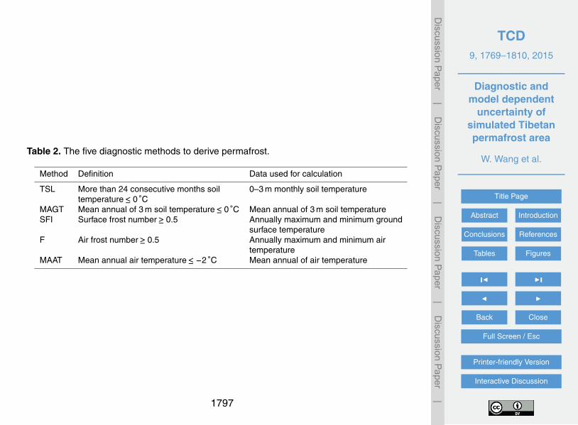
All the 5 diagnostic methods are summarized in Table 2. The three direct methods(TSL, MAGT, SFI) are based on simulated ground temperatures, while the two indirect20

methods (F and MAAT) use the prescribed air temperature. SFI is mainly controlled byair temperature and snow cover, but it also depends on how the soil is parameterized,so SFI is somewhat closer to the indirect methods than are TSL and MAGT.

The 3 methods introduced in the 1980s (SFI, F, MAAT), were designed to map per-mafrost based on the assumption that the permafrost distribution is related to climatic25

parameters. Although permafrost processes are directly represented in climate modelsnowadays, the simulated soil temperatures have considerable errors, and the directlydiagnosed permafrost area has model-dependent biases (Koven et al., 2013; Slater

1777





TCD9, 1769–1810, 2015



W. Wang et al.

Title Page



Tables Figures

J I

J I

Back Close

Full Screen / Esc



Discussion

Paper

|D

iscussionP

aper|

Discussion

Paper

|D

iscussionP

aper|

and Lawrence, 2013). Therefore the older indirect diagnostic methods are also still verycommonly used (e.g., Wang et al., 2006; Jin et al., 2007; Ran et al., 2012; Nan et al.,2012; Slater and Lawrence, 2013; Saito, 2013; Koven et al., 2013). TP permafrost areadirectly diagnosed from the simulated monthly soil temperatures (TSL) is not supe-rior to the other methods in comparison with the observation-derived permafrost map5

(Figs. 1 and 2). Hence, we consider all the 5 diagnostic methods to quantify the fullrange of uncertainty in the model-derived permafrost maps.

Since the forcing air temperatures of LSMs were not the same due to discrepanciesin the historical temperature (and precipitation and other forcing fields) datasets usedby the individual models (Table 1), we use the indirect methods to quantify forcing10

differences. If these differences are not too large, we can attribute the differences inthe direct method-derived permafrost areas primarily to differences of modeled landsurface processes. Across-model and across-method variability is listed in Table 3. Aswe use fairly small numbers of methods and models, rather than defining uncertainty interms of SD, we choose to use the full range of values from the simulations and define15

uncertainty as maximum-minimum values among the models.

3 Data and analysis approach

3.1 Data from stand-alone LSMs

Output from six stand-alone LSMs participating in the inter-model comparisonproject “Vulnerability of Permafrost Carbon Research Coordination Network (RCN-20

Permafrost)” (http://www.permafrostcarbon.org/) is analyzed in this study (Table 1). Thesimulations have been generally conducted for recent decades from 1960 to 2009 usingmonthly resolution climate forcing input data. Each modeling team was free to chooseappropriate driving data sets for climate, atmospheric CO2, N deposition, disturbance,soil texture, etc., as used in their standard modeling system. The LSMs use different25

horizontal model resolutions and different soil layer divisions (Table 1). We also ana-

1778





http://www.permafrostcarbon.org/

TCD9, 1769–1810, 2015



W. Wang et al.

Title Page



Tables Figures

J I

J I

Back Close

Full Screen / Esc



Discussion

Paper

|D

iscussionP

aper|

Discussion

Paper

|D

iscussionP

aper|

lyzed (but do not show here) output from a coupled earth-system model (Miroc-ESM).In contrast with the land surface models we present here, the Miroc-ESM coupledmodel generates its own air temperatures, which over TP, were 4–8 ◦C cooler thantemperatures in the other driving datasets. This creates issues with other model fieldssuch as snow thickness and albedo which make comparison of permafrost processes5

more difficult than with the stand-alone LSMs.Our analysis is based on monthly averages of the driving air temperature and simu-

lated ground temperature. As three models (CoLM, JULES and LPJ-GUESS; Table 1)have shallow soil layers, we restrict our analysis to the common depth range spanningnear surface to 3 m. Ground temperatures were interpolated onto the common depths:10

0.05, 0.1, 0.2, 0.5, 1, 2, 3 m. Since there is no ground surface temperature output, weextrapolate the below soil temperatures onto the ground surface. Most TP permafrostwork has been post-1980 (Guo and Wang, 2013; Nan et al., 2012), so we choose 1980as the start of the analysis period. The end is limited to the year 2000 by results fromthe JULES model (Table 1).15

3.2 TP permafrost observation-based map

Mapping permafrost on TP is challenging due to absence of field observations, es-pecially in the central and western parts where permafrost is widespread. In practice,permafrost maps on TP have been statistical models based on a compilation of earliermaps, aerial photographs, Landsat images and terrain analysis (Ran et al., 2012; Shi20

et al., 1988; Li and Cheng, 1996; Nan et al., 2002) as well as on some MAGT and MAATdata from the few long-term monitoring sites (Ran et al., 2012; Wang et al., 2006). Theclassification and therefore the mapping of TP permafrost is not consistent across thedifferent studies (Ran et al., 2012).

The mostly widely used map by Li and Cheng (1996) has large differences from other25

maps, and shows excess permafrost in the southeast where permafrost can only existon extremely cold mountains (Gruber, 2012). The International Permafrost Association(IPA) map (Brown et al., 1997; Heginbottom, 2002) is the most widely used in NH

1779





TCD9, 1769–1810, 2015



W. Wang et al.

Title Page



Tables Figures

J I

J I

Back Close

Full Screen / Esc



Discussion

Paper

|D

iscussionP

aper|

Discussion

Paper

|D

iscussionP

aper|

permafrost analysis. However, the IPA map is not well suited for TP because the dataand information in this map is based on the map made by Shi et al. (1988) which hasnot been updated since.

We use the 1 : 4 000 000 Map of the Glaciers, Frozen Ground and Deserts in China(Wang et al., 2006, hereafter refered to as the “Wang06 map”) as the primary ref-5

erence. The map is based on MAGT (Nan et al., 2002) with 0.5 ◦C as the boundarybetween permafrost and seasonally frozen ground. Nan (2002) fitted a multiple linearregression between latitude, altitude and MAGT, from all 76 TP stations having bore-hole data, and extrapolated this regression to the whole TP with a 1 km resolution DEMto get the MAGT distribution. The Wang06 map was re-gridded to match the different10

model resolutions and spatial domain (see observation column in Fig. 1), and the dif-ferent permafrost areas derived from the methods and models are compared with theWang06 map in Fig. 2.

We emphasize that the Wang06 map is subject to uncertainty as it is based on a rel-atively sparse set of observations and then statistical extrapolation. Nan et al. (2013)15

pointed out that permafrost was overestimated in the western TP in both the maps by Liand Cheng (1996) and Wang et al. (2006). However, a better permafrost map coveringthe whole TP is not available.

3.3 Measure of agreement between simulated and Wang06 permafrost maps

To evaluate the agreement of simulated permafrost map with the Wang06 map, we20

calculate the Kappa coefficient (Cohen, 1960; Monserud and Leemans, 1992; Wang,2010), K , which measures the degree of agreement between two maps.

K =

(s/n− (a1b1 +a0b0)/n2

)(1− (a1b1 +a0b0)/n2

) (3)

where the total number of the map points is n, and s is the number of points wheresimulation and observational estimate agree. The numbers of Wang06 map cells with25

1780





TCD9, 1769–1810, 2015



W. Wang et al.

Title Page



Tables Figures

J I

J I

Back Close

Full Screen / Esc



Discussion

Paper

|D

iscussionP

aper|

Discussion

Paper

|D

iscussionP

aper|

permafrost is a1, and those without are a0, and the corresponding simulated map cellnumbers are b1 and b0. The calculated K matrix of simulated and Wang06 permafrostmaps is presented in Fig. 3. Empirically, and statistically arbitrary quality values for Khave been proposed (e.g. Cohen, 1960), who suggested that K ≥ 0.8 signifies excellentagreement, 0.6 ≤ K < 0.8 represents substantial agreement, 0.4 ≤ K < 0.6 represents5

moderate agreement, 0.2 ≤ K < 0.4 represents fair agreement, while lack of agreementcorresponds to K < 0.2. There is a sample size issue in estimating the confidence ofK and this can be a factor when very small numbers of grid points are available (herethis applies to UVic).

3.4 Data used to examine model thermal structures10

The derived permafrost maps depend on the modeled ground thermal structures. How-ever, field studies on TP are quite limited, and we have only short duration (1996–2000) ground temperature profiles obtained from the GEWEX Asian Monsoon Experi-ment (GAME)-Tibet (Yang et al., 2003) at three permafrost stations (D66, D105, D110;Fig. 1) in the central TP to compare with model results. We present the top (0.04 m) and15

deeper (2.63 or 3 m) soil layer temperatures (modeled temperatures were weighted bi-linear interpolated onto the station locations) in Fig. 4 and Table 4. We also give a shortdescription of the sites vegetation and soil texture information, both from observationand models.

We also analyze monthly air and ground temperatures in a selected area in the west-20

ern TP (33–36◦ N, 82.5–85.5◦ E, Fig. 1) to examine across-model differences (Fig. 5).As this region is the coldest part of TP (according to the annual mean air temperature)the permafrost is widely distributed, and the active layer thickness is less than 3 m.However, TSL method derived permafrost areas vary significantly among the modelsin this area (Fig. 1). Despite the lack of any ground temperature observations in this25

area, the definite presence of permafrost makes it useful to look at the ground ther-mal structure of each model as well as their differences as a means of interpreting thecalculated permafrost areas.

1781





TCD9, 1769–1810, 2015



W. Wang et al.

Title Page



Tables Figures

J I

J I

Back Close

Full Screen / Esc



Discussion

Paper

|D

iscussionP

aper|

Discussion

Paper

|D

iscussionP

aper|

4 Results

4.1 Uncertainties in air-temperature-derived permafrost area

Air temperature–derived permafrost maps are investigated with the two indirect meth-ods, F and MAAT. Figures 1 and 2 compare both Wang06 and model-derived per-mafrost maps, and show that F produces consistently excessive permafrost area com-5

pared with MAAT. That is because the empirical threshold of −2 ◦C for MAAT fits wellwith TP observations (Xu et al., 2001), while F ≥ 0.5 is a theoretical assumption, whichhas been reported to overestimate permafrost area (Nelson and Outcalt, 1987; Slaterand Lawrence, 2013). Accordingly, Fig. 3 shows that F derived permafrost is less con-sistent with observation (model average K = 0.3 for the common region) than MAAT-10

derived permafrost area (K = 0.5).Across-model variability (Table 3) for the MAAT-based method is 14×104 km2 and

for the F based method is 17×104 km2, equivalent to about 14–17 % of the Wang06permafrost area inside the common modeling region (101×104 km2). This variability ismuch smaller than the 56 % calculated by Slater and Lawrence (2013) for the CMIP515

models with the SFI∗ method for NH permafrost area. The relatively smaller differenceamong the models here is because, although the temperature forcing was not identicalamong models, the mean annual air temperature and its spatial variability in the per-mafrost region are quite similar (between −6 and −8 ◦C). Hence most of the differencesamong the indirect methods that use air temperature to derive permafrost area can be20

attributed to different model horizontal resolutions. Since the differences in permafrostextent using the air temperature based indirect methods are relatively small, the dif-ferences in the direct method derived extents can primarily be attributed to the LSMsstructural and parametric differences.

1782





TCD9, 1769–1810, 2015



W. Wang et al.

Title Page



Tables Figures

J I

J I

Back Close

Full Screen / Esc



Discussion

Paper

|D

iscussionP

aper|

Discussion

Paper

|D

iscussionP

aper|

4.2 Uncertainties in model–derived permafrost area

There is a large across-model variability of permafrost area derived from direct meth-ods (TSL, MAGT and SFI) (Figs. 1 and 2; 111–120× 104 km2; Table 3) and it is similarfor all the 3 diagnosis methods. This across-model variability is much larger than thevariability using the indirect methods discussed in Sect. 4.1, and is equivalent to 110–5

112 % of Wang06 permafrost area for the common modeling region. CMIP5 across-model variability derived from TSL in NH permafrost area was similarly large (Slaterand Lawrence, 2013; Koven, 2013). Clearly this points to large across-model differ-ences in ground thermal structures.

The across-method (TSL, MAGT and SFI) variability in permafrost area (Figs. 1 and10

2; Table 3) is very variable between models: UVic and LPJ-GUESS have smallestranges (up to 9×104 km2), while CoLM has the largest (87×104 km2) (Table 3), near tothe total permafrost area of the common region. Thus the across-direct method rangeis similar to the across-model range. Slater and Lawrence (2013) also emphasized thevariable across-method variability for NH permafrost area between models, however15

Saito (2013) showed insignificant variability across both direct and indirect methods forderived pre-industrial NH continuous permafrost area.

4.3 Model evaluation based on K and ground temperature profile

A good land surface model should adequately simulate the seasonal and annualground temperature profiles. Hence one quality test for a model is that it should be20

able to produce “good” permafrost maps, which we define as agreement with theobservation-based map, based on all the three direct diagnostic methods. The ap-plied criterion is the kappa coefficient K (Sect. 3.3). If we take the (arbitrary) thresholdK ≥ 0.4 (indicating “moderate agreement”), then no model passes this test for the com-mon simulation region, while reducing the threshold to K ≥ 0.2 (“fair agreement”) allows25

most models and methods to pass while UVic stands out as a clear failure (Fig. 3).

1783





TCD9, 1769–1810, 2015



W. Wang et al.

Title Page



Tables Figures

J I

J I

Back Close

Full Screen / Esc



Discussion

Paper

|D

iscussionP

aper|

Discussion

Paper

|D

iscussionP

aper|

If the criterion for acceptable model bias is ≤±2.0 ◦C, then simulations of mean an-nual ground temperatures from most models (CLM4.5, CoLM, ISBA and JULES) agreewith the observations, but only the simulation of seasonal cycle amplitude of one model(ISBA) agrees with observations. However, if the criterion is bias≤±1.0 ◦C, then nomodel agrees with observations for neither mean annual ground temperature nor the5

seasonal cycle amplitude (Fig. 4, Table 4).We now look at the performance of the 2 models with larger biases in mean annual

ground temperature: LPJ-GUESS and UVic. LPJ-GUESS simulated too cold (by morethan 3 ◦C) mean annual ground temperatures for both the surface and deeper layers(Fig. 4, Table 4). The summer temperatures simulated by the model in the surface10

layers are especially cold, with maximum temperatures lower than observation by 8 ◦C(Fig. 4a and c) and its ground temperature amplitude is substantially underestimated(Table 4), which must greatly limit the summer thaw depth. This cold soil results insubstantial overestimation of permafrost area (119–131×104 km2; Table 3, Fig. 2) withsmall across-method variability.15

UVic simulates a soil thermal state that is the warmest among the models, with thesimulated mean annual ground temperature at D66 surpassing observation by morethan 7 ◦C (Fig. 4, Table 4). If the observational sites are representative then the gener-ally too warm ground temperature in UVic is the reason for the extremely small simu-lated permafrost area (8×104 km2; Table 3, Fig. 2) with all direct methods, and hence20

to no across-method variability, and poor agreement with the Wang06 permafrost map(K < 0.1; Fig. 3).

4.4 Method comparison based on K and ground temperature profile

Permafrost maps derived using MAGT and SFI often show larger area than TSL(Fig. 2), with generally better agreement with the Wang06 map (Fig. 3). The MAGT25

method simply defines a grid as permafrost as long as its 3 m mean annual groundtemperature is colder than 0 ◦C, and a permafrost threshold value of SFI≥ 0.5 alsoonly requires the mean annual ground surface temperature is lower than 0 ◦C (Nan,

1784





TCD9, 1769–1810, 2015



W. Wang et al.

Title Page



Tables Figures

J I

J I

Back Close

Full Screen / Esc



Discussion

Paper

|D

iscussionP

aper|

Discussion

Paper

|D

iscussionP

aper|

2012). Figures 4 and 5 show most models meet these criteria. However, assuming thatthe site observations are representative, the simulated mean annual ground tempera-tures of both surface and deeper soil layers often have obvious biases (≥±1 ◦C) in allthe models (Fig. 4 and Table 4).

In general, model-derived permafrost distribution using the TSL method shows little5

agreement with the Wang06 map (Figs. 1–3). In contrast with MAGT and SFI methods,the TSL method requires adequate simulation of both mean annual ground temperatureand the seasonal cycle at monthly resolution (Fig. 4, Table 4). This means that the TSLmethod is more susceptible to model errors, but it offers a more comprehensive insightinto land model processes. CoLM is an extreme example of how a simulated permafrost10

map can be totally incorrect due to small errors in seasonal ground temperature. CoLMsimulates nearly no TSL -derived permafrost (Figs. 1 and 2), accounting for much ofthe large across-model and across-method variability (Table 3). This is despite CoLMhaving lower mean annual ground temperatures for the 3 m layer than many othermodels (ISBA, CLM4.5 and JULES). However, it simulates a larger seasonal amplitude15

than CLM4.5 and ISBA (Fig. 5), so that, in the western TP, the monthly maximum3 m ground temperatures in CoLM always surpasses 0 ◦C by around 0.2 ◦C (Fig. 5c)precluding it being classed as permafrost with the TSL method.

5 Discussion of the related main processes causing ground temperaturediscrepancies20

In comparison with site observations, the most noticeable ground temperature discrep-ancies of the 6 models discussed in Sect. 4 and relevant for the most biased simulatedpermafrost area are the underestimation of soil temperature by LPJ-GUESS and theoverestimation of soil temperature by UVic. There are many other, rather subtle, poten-tial model discrepancies that we do not investigate in detail here. One example is the25

overestimation of the amplitude of the seasonal temperature cycle at deep depths inseveral models (Fig. 4b and d; Table 4). Table 4 also shows that the observed vegeta-

1785





TCD9, 1769–1810, 2015



W. Wang et al.

Title Page



Tables Figures

J I

J I

Back Close

Full Screen / Esc



Discussion

Paper

|D

iscussionP

aper|

Discussion

Paper

|D

iscussionP

aper|

tion and soil texture are mis-matched by all the models at each of the stations. Althoughit is a common problem to compare grid cell results against site data, model descriptionof vegetation and soil texture is too simplified.

To help elucidate the causes of ground temperature discrepancies associated withsoil processes we also inspect snow depth and vertical ground temperature gradi-5

ents. We use the Long Time Series Snow Dataset of China (Che et al., 2008) (http://westdc.westgis.ac.cn) to examine the modeled snow depth. The complete datasetis composed of SMMR (1978–1987), SSM/I (1987–2008) and AMSR-E (2002–2010).Here we use the data of SMMR and SSM/I to produce the winter (DJF) climatologi-cal distribution of 1980–2000 (Fig. 6). Furthermore, we follow Koven et al. (2013) and10

calculated two vertical gradients to isolate processes: from the atmosphere to groundsurface (Fig. 7) and from ground surface to deeper soil (at 1 m depth) (Fig. 8). Whilethe first one is mainly controlled by the snow insulation, the latter is mainly determinedby soil hydrology, latent heat and thermal properties. Important factors that influencethe ground thermal structure are compared in Table 5. Since several models produce15

incomplete or not directly comparable output, we restrict ourselves to a qualitative as-sessment here.

The LPJ-GUESS simulated underestimation of soil temperature is not caused bya bias in the surface air temperature forcing (Fig. 5, Table 4). Instead, this bias may bedue to many factors such as inappropriate prescriptions of soil thermal properties, poor20

representation of soil hydrology, and mis-match of vegetation types. Figure 8 showsthat the soil temperatures increase with depth, but LPJ-GUESS has a much smallertemperature gradient between the surface and the 1 m deep soil (0–2 K) than the othermodels. This suggests a different (larger) winter soil thermal conductivity probably as-sociated with a high soil porosity and water content. LPJ-GUESS specifies the same25

soil texture for the TP as for the Arctic, which is mostly clay-like (Table 4). Clay has highwater retention capacity. Many studies have reported that the soil on TP is immature,with coarser particles than typical for Arctic permafrost and with much less organicmatter. Inappropriate soil texture classification will affect the simulated ground thermal

1786





http://westdc.westgis.ac.cn



TCD9, 1769–1810, 2015



W. Wang et al.

Title Page



Tables Figures

J I

J I

Back Close

Full Screen / Esc



Discussion

Paper

|D

iscussionP

aper|

Discussion

Paper

|D

iscussionP

aper|

structure. LPJ-GUESS underestimates the surface and top soil temperatures particu-larly in summer (Figs. 4a and c, 5). Precipitation and hydrological processes determinethe vertical profile of soil water content which can change the fraction of water and iceretained in different soil layers and influence soil thermal conduction. The energy re-quired to melt the high water (ice) content in the surface soil layers in summer appears5

to lead underestimated low summer temperatures compared with other models, anda phase lag in summer warming (Fig. 4a and c).

UVic uses the same climate forcing as CLM4.5 (Table 1), but simulates much warmerground temperatures than other models. In contrast with the other models, UVic hasno snow cover in winter (Fig. 6), which is consistent with grid cell surface albedo being10

year-round at values between 0.15–0.35. The simulated snow depth is derived from theprescribed winter precipitation, and the model’s snow, energy and water balances. Thelack of snow over TP in UVic likely indicates removal by sublimation. A too low snowalbedo makes the snow gain energy that is lost through sublimation. Since it takesmore energy to sublimate snow than it does to melt it, the latent heat flux should be,15

and is (not shown) higher in UVic than other models. However, despite the apparentsnow sublimation – which should cool the soil, the ground surface temperatures in UVicare warmer than in all the models. The large absorption of short wave radiation allowedby the year-round low albedo provides this heat and is sufficient for there to be verylittle permafrost simulated by UVic for the TP.20

ISBA, and especially JULES stand out from other models in their calculated wintertemperature offsets: ground surface temperatures are colder than the driving air tem-peratures over much of the simulated region (Fig. 7), and in those places the deep soiltemperatures are relatively warmer (Fig. 8). Snow (Fig. 6) and vegetation cover shouldprovide insulation making soil warmer than air temperatures in winter, thus the nega-25

tive temperature offsets are not physically consistent. Snow depth for the two modelsis thick enough to produce a warming effect (Fig. 6). This suggests problems with sur-face insulation which, to a degree, is compensated for by an anomalous soil thermalconductivity that maintains deep soil warmth in those regions with a negative insulation

1787





TCD9, 1769–1810, 2015



W. Wang et al.

Title Page



Tables Figures

J I

J I

Back Close

Full Screen / Esc



Discussion

Paper

|D

iscussionP

aper|

Discussion

Paper

|D

iscussionP

aper|

effect. Hence, although the permafrost maps produced by the models have a K > 0.2compared with the observation-based Wang06 map, there are problems with the sur-face and soil temperature profiles.

6 Summary and conclusions

Results of this model intercomparison quantify, for the first time, the uncertainties of5

model derived permafrost area on the Tibetan Plateau (TP). The uncertainties stemfrom across-model and across-diagnostic method variability as well as historic climatedata uncertainties. According to the agreement of the air temperature based diagnos-tic methods (MAAT and F), we found lower uncertainty in permafrost area associatedwith air temperature forcing (99–135×104 km2) in comparison with the uncertainty (1–10

128×104 km2) associated with the simulation of soil temperature used in the other threediagnostic methods (TSL, MAGT, and SFI); observation-based Wang06 permafrostarea is 101×104 km2.

The models in this study generally produced permafrost maps in better agreementwith the Wang06 map using the MAGT and SFI methods rather than with the TSL15

method. But this does not mean that the models simulate permafrost dynamics cor-rectly. Although most models can capture the threshold value of MAGT and SFI, theirground temperatures still show various biases, both in the mean annual value and theseasonal variation. Therefore, most models produce worse permafrost maps with theTSL method. The TSL method is a more demanding, and to date, elusive target.20

Modeled snow depth and surface and soil temperature offsets vary widely amongstthe models. If the observation sites for soil temperature are representative, then LPJ-GUESS and UVic have substantial biases in their soil temperature simulations, mainlyattributable to inappropriate description of the surface (vegetation, snow cover) and soilproperties (soil texture, hydrology). Other models (ISBA, JULES) show biases in the25

simulation of winter soil temperature.

1788





TCD9, 1769–1810, 2015



W. Wang et al.

Title Page



Tables Figures

J I

J I

Back Close

Full Screen / Esc



Discussion

Paper

|D

iscussionP

aper|

Discussion

Paper

|D

iscussionP

aper|

From investigations in the arctic and boreal regions, we know that the specification ofsurface and soil properties needs substantial improvement. In addition, models needto consider deeper soil columns in their simulations. Nicolsky et al. (2007) recommenda soil column of at least 80 m for models applied to arctic and boreal regions. Thepermafrost in the TP is usually much warmer and with a deeper active layer than found5

in continuous permafrost of the arctic and boreal region, hence deep soil layers wouldalso be applicable for TP permafrost simulation. A shallow column in a permafrostmodel can cause problems in the simulation of the degradation of warm permafrost(near 0 ◦C), which is expected for projections of future climate warming (Alexeev et al.,2007; Lawrence et al., 2008).10

Further evaluation of model results from the permafrost-RCN is underway for TP thatexamines permafrost temperature, active layer thickness and carbon balance underpresent and future climate forcing. We also plan to complement this model intercom-parison study by an uncertainty quantification analysis of key model parameters (e.g.improved vegetation and snow albedo, soil colors, etc) with the CoLM model. However,15

a crucial requirement for this is much better data availability allowing for better spatialcoverage across the TP in the evaluation of simulated ground temperature profiles. Un-der the Chinese Scientific Foundation Project “Permafrost Background Investigation onthe Tibetan Plateau” (No. 2010CB951402), a series of new stations have been estab-lished, especially in the depopulated zone. More ground truth data will be published in20

the near future, which will also be assimilated in a new observation-based permafrostmap.

Acknowledgements. This study was supported by the Permafrost Carbon Vulnerability Re-search Coordination Network, which is funded by the National Science Foundation. Any useof trade, firm, or product names is for descriptive purposes only and does not imply endorse-25

ment by the US Government. E. Burke was supported by the Joint UK DECC/Defra Met OfficeHadley Centre Climate Programme (GA01101) and the European Union Seventh FrameworkProgramme (FP7/2007-2013) under grant agreement n◦ 282700. This research was also spon-sored by Chinese foundations: (1) the National Basic Research Program of China (Grant No.2015CB953600), (2) the National Science Foundation of China (Grant No. 40905047), (3) the30

1789





TCD9, 1769–1810, 2015



W. Wang et al.

Title Page



Tables Figures

J I

J I

Back Close

Full Screen / Esc



Discussion

Paper

|D

iscussionP

aper|

Discussion

Paper

|D

iscussionP

aper|

National Natural Science Foundation of China (Grant No.41275003), and (4) the National Nat-ural Science Foundation of China (Grant No.41030106).

References

Alexeev, V., Nicolsky, D., Romanovsky, V., and Lawrence, D.: An evaluation of deep soil con-figurations in the CLM3 for improved representation of permafrost, Geophys. Res. Lett., 34,5

L09502, doi:10.1029/2007GL029536, 2007.AWFA: Data Format Handbook for AGRMET, available at: http://www.mmm.ucar.~edu/mm5/

documents/data_format_handbook.pdf (last access: 20 January 2010), 2002.Brown, J., Ferrians, O., Heginbottom, J., and Melnikov, E.: Circum-Arctic Map of Permafrost

and Ground-Ice Conditions, US Geological Survey, Reston, USA, 1997.10

Che, T., Li, X., Jin, R., Armstrong, R., and Zhang, T. J.: Snow depth derived from passivemicrowave remote-sensing data in China, Ann. Glaciol., 49, 145–154, 2008.

Cheng, G. and Jin, H.: Permafrost and groundwater on the Qinghai-Tibet Plateau and in north-east China[J], Hydrogeol. J., 21, 5–23, 2013.

Cohen, J.: A coefficient of agreement for nominal scales, Educ. Psychol. Meas., 20, 37–46,15

1960.Dankers, R., Burke, E. J., and Price, J.: Simulation of permafrost and seasonal thaw depth in

the JULES land surface scheme, The Cryosphere, 5, 773–790, doi:10.5194/tc-5-773-2011,2011.

Dörfer, C., Kühn, P., Baumann, F., He, J., and Scholten, T.: Soil organic carbon pools20

and stocks in permafrost-affected soils on the Tibetan Plateau, PloS One, 8, e57024,doi:10.1371/journal.pone.0057024, 2013.

Essery, R., Morin, S., Lejeune, Y., and Ménard, C. B.: A comparison of 1701 snowmodels using observations from an alpine site, Adv. Water Resour., 55, 131–148,doi:10.1016/j.advwatres.2012.07.013, 2013.25

Gruber, S.: Derivation and analysis of a high-resolution estimate of global permafrost zonation,The Cryosphere, 6, 221–233, doi:10.5194/tc-6-221-2012, 2012.

Gubler, S., Endrizzi, S., Gruber, S., and Purves, R. S.: Sensitivities and uncertainties of mod-eled ground temperatures in mountain environments, Geosci. Model Dev., 6, 1319–1336,doi:10.5194/gmd-6-1319-2013, 2013.30

1790





http://dx.doi.org/10.1029/2007GL029536

http://www.mmm.ucar.~edu/mm5/documents/data_format_handbook.pdf



http://dx.doi.org/10.5194/tc-5-773-2011

http://dx.doi.org/10.1371/journal.pone.0057024

http://dx.doi.org/10.1016/j.advwatres.2012.07.013

http://dx.doi.org/10.5194/tc-6-221-2012

http://dx.doi.org/10.5194/gmd-6-1319-2013

TCD9, 1769–1810, 2015



W. Wang et al.

Title Page



Tables Figures

J I

J I

Back Close

Full Screen / Esc



Discussion

Paper

|D

iscussionP

aper|

Discussion

Paper

|D

iscussionP

aper|

Guo, D. and Yang, M.: Simulation of Soil Temperature and Moisture in Seasonally FrozenGround of Central Tibetan Plateau by SHAW Model, Plateau Meteorology, 29, 1369–1377,2010.

Guo, D. and Wang, H.: Simulation of permafrost and seasonally frozen ground conditions onthe Tibetan Plateau, 1981–2010, J. Geophys. Res.-Atmos., 118, 5216–5230, 2013.5

Guo, D., Wang, H., and Li, D.: A projection of permafrost degradation on the Ti-betan Plateau during the 21st century, J. Geophys. Res.-Atmos., 117, D05106,doi:10.1029/2011JD016545, 2012.

Heginbottom, J.: Permafrost mapping: a review, Prog. Phys. Geog., 26, 623–642, 2002.Hillel, D.: Environmental Soil Physics: Fundamentals, Applications, and Environmental Consid-10

erations, Academic Press, New York, USA, 1998.IPCC: Climate Change 2013: the Physical Science Basis Contribution of Working Group I to

the Fifth Assessment Report of the Intergovernmental Panel on Climate Change, CambridgeUniversity Press, Cambridge, 2013.

Ji, D., Wang, L., Feng, J., Wu, Q., Cheng, H., Zhang, Q., Yang, J., Dong, W., Dai, Y., Gong, D.,15

Zhang, R.-H., Wang, X., Liu, J., Moore, J. C., Chen, D., and Zhou, M.: Description and basicevaluation of Beijing Normal University Earth System Model (BNU-ESM) version 1, Geosci.Model Dev., 7, 2039–2064, doi:10.5194/gmd-7-2039-2014, 2014.

Jin, H., Yu, Q., Lü, L., Guo, D., He, R., Yu, S., Sun, G., and Li, Y.: Degradation of permafrost inthe Xing’anling Mountains, Northeastern China, Permafrost Periglac., 18, 245–258, 2007.20

Koven, C., Riley, W., and Stern, A.: Analysis of permafrost thermal dynamics and response toclimate change in the CMIP5 Earth System Models, J. Climate, 26, 1877–1900, 2013.

Lawrence, D. and Slater, A.: A projection of severe near-surface permafrost degradation duringthe 21st century, Geophys. Res. Lett., 32, L24401, doi:10.1029/2005GL025080, 2005.

Lawrence, D., Slater, A., Romanovsky, V., and Nicolsky, D.: The sensitivity of a model projection25

of near-surface permafrost degradation to soil column depth and inclusion of soil organicmatter, J. Geophys. Res., 113, F02011, doi:10.1029/2007JF000883, 2008.

Li, Q., Sun, S., and Dai, Q.: The numerical scheme development of a simplified frozen soilmodel, Adv. Atmos. Sci., 26, 940–950, 2009.

Li, S. and Cheng, G.: Map of Frozen Ground on Qinghai-Xizang Plateau, Gansu Culture Press,30

Lanzhou, 1996.

1791





http://dx.doi.org/10.1029/2011JD016545

http://dx.doi.org/10.5194/gmd-7-2039-2014

http://dx.doi.org/10.1029/2005GL025080

http://dx.doi.org/10.1029/2007JF000883

TCD9, 1769–1810, 2015



W. Wang et al.

Title Page



Tables Figures

J I

J I

Back Close

Full Screen / Esc



Discussion

Paper

|D

iscussionP

aper|

Discussion

Paper

|D

iscussionP

aper|

Li, S., Gao, S., Yang, P., and Chen, H.: Some problems of freeze–thaw desertification in theQinghai-Tibetan Plateau: a case study on the desertification regions in the western andnorthern Tibet, J. Glaciol. Geocryol., 27, 476–485, 2005.

Li, Z., Tang, P., Zhou, J., Tian, B., Chen, Q., and Fu, S.: Permafrost environment monitoring onthe Qinghai-Tibet Plateau using time series ASAR images, International Journal of Digital5

Earth, doi:10.1080/17538947.2014.923943, online, first, 2014.Luo, S., Lv, S., Zhang, Y., Hu, Z., Ma, Y., Li, S., and Shang, L.: Simulation analysis on land

surface process of BJ site of central Tibetan Plateau using CoLM, Plateau Meteorology, 27,259–271, 2008.

Monserud, R. and Leemans, R.: Comparing global vegetation maps with the Kappa statistic,10

Ecol. Model., 62, 275–293, 1992.Nan, Z., Li, S., and Liu, Y.: Mean annual ground temperature distribution on the Tibetan Plateau:

permafrost distribution mapping and further application, J. Glaciol. Geocryol., 24, 142–148,2002.

Nan, Z., Li, S., Cheng, G., and Huang, P.: Surface frost number model and its application to the15

Tibetan plateau, J. Glaciol. Geocryol., 34, 89–95, 2012.Nan, Z., Huang, P., and Zhao, L.: Permafrost distribution modeling and depth estimation in the

Western Qinghai-Tibet Plateau, Acta Geographica Sinica, 68, 318–327, 2013.Nelson, F. and Outcalt, S.: A computational method for prediction and regionalization of per-

mafrost, Arctic Alpine Res., 19, 279–288, 1987.20

Nicolsky, D. J., Romanovsky, V. E., Alexeev, V. A., and Lawrence, D. M.: Improved modelingof permafrost dynamics in a GCM land-surface scheme, Geophys. Res. Lett., 34, L08501,doi:10.1029/2007GL029525, 2007.

Qin, J., Yang, K., Liang, S., Zhang, H., Ma, Y., Guo, X., and Chen, Z.: Evaluation of surfacealbedo from GEWEX-SRB and ISCCP-FD data against validated MODIS product over the25

Tibetan Plateau, J. Geophys. Res.-Atmos., 116, D24116, doi:10.1029/2011JD015823, 2011.Ran, Y., Li, X., Cheng, G., Zhang, T., Wu, Q., Jin, H., and Jin, R.: Distribution of permafrost in

China: an overview of existing permafrost maps, Permafrost Periglac., 23, 322–333, 2012.Saito, K., Sueyoshi, T., Marchenko, S., Romanovsky, V., Otto-Bliesner, B., Walsh, J.,

Bigelow, N., Hendricks, A., and Yoshikawa, K.: LGM permafrost distribution: how well can30

the latest PMIP multi-model ensembles perform reconstruction?, Clim. Past, 9, 1697–1714,doi:10.5194/cp-9-1697-2013, 2013.

1792





http://dx.doi.org/10.1080/17538947.2014.923943

http://dx.doi.org/10.1029/2007GL029525

http://dx.doi.org/10.1029/2011JD015823

http://dx.doi.org/10.5194/cp-9-1697-2013

TCD9, 1769–1810, 2015



W. Wang et al.

Title Page



Tables Figures

J I

J I

Back Close

Full Screen / Esc



Discussion

Paper

|D

iscussionP

aper|

Discussion

Paper

|D

iscussionP

aper|

Schuur, E. A., Bockheim, J., Canadell, J. G., Euskirchen, E., Field, C. B., Goryachkin, S. V.,Hagemann, S., Kuhry, P., Lafleur, P. M., and Lee, H.: Vulnerability of permafrost carbon toclimate change: implications for the global carbon cycle, BioScience, 58, 701–714, 2008.

Shi, Y., Mi, D., Feng, Q., Li, P., and Wang, Z.: Map of Snow, Ice and Frozen Ground in China,China Cartographic Publishing House, Beijing, China, 1988.5

Slater, A. and Lawrence, D.: Diagnosing present and future permafrost from climate models, J.Climate, 26, 5608–5623, doi:10.1175/JCLI-D-12-00341.1, 2013.

Tian, L., Li, W., Zhang, R., Tian, L., Zhu, Q., Peng, C., and Chen, H.: The analysis of snowinformation from 1979 to 2007 in Qinghai-Tibetan Plateau, Acta Ecologica Sinica, 34, 5974–5983, 2014.10

Van, D.: Influence of Soil Management on the Temperature Wave Near the Soil Surface, Tech.Bull. 29, Institute of Land and Water Manage. Res., Wageningen, Netherlands, 21 pp., 1963.

Wang, C. and Shi, R.: Simulation of the land surface processes in the Western Tibetan Plateauin summer, J. Glaciol. Geocryol., 29, 73–81, 2007.

Wang, G., Li, Y., Wang, Y., and Wu, Q.: Effects of permafrost thawing on vegetation and soil15

carbon pool losses on the Qinghai-Tibet Plateau, China, Geoderma, 143, 143–152, 2008.Wang, K., Cheng, G., Jiang, C., and Niu, F.: Variation of thermal diffusivity and temperature sim-

ulation of soils of vertical heterogeneity in Nagqu Prefecture in the Tibetan Plateau, Journalof Glaciology and Geocryology, 29, 470–474, 2007.

Wang, T., Wang, N. L., and Li, S. X.: Map of the Glaciers, Frozen Ground and Desert in China,20

1 : 4 000 000 (in Chinese), Chinese Map Press, Beijing, China, 2006.Wang, X., Yang, M., and Wan, G.: Processes of soil thawing-freezing and features of ground

temperature and moisture at D105 on the Northern Tibetan Plateau, J. Glaciol. Geocryol.,34, 56–63, 2012.

Wang, Z.: Applications of permafrost distribution models on the Qinghai-Tibetan Plateau,25

Lanzhou University, China, 2010.Wu, Q. and Liu, Y.: Ground temperature monitoring and its recent change in Qinghai-Tibet

Plateau, Cold Reg. Sci. Technol., 38, 85–92, 2004.Wu, Q. and Niu, F.: Permafrost changes and engineering stability in Qinghai-Xizang Plateau,

Chinese Sci. Bull., 58, 1079–1094, 2013.30

Wu, Q. and Zhang, T.: Changes in active layer thickness over the Qinghai-Tibetan Plateau from1995 to 2007, J. Geophys. Res.-Atmos., 115, D09107, doi:10.1029/2009JD012974, 2010.

1793





http://dx.doi.org/10.1175/JCLI-D-12-00341.1

http://dx.doi.org/10.1029/2009JD012974

TCD9, 1769–1810, 2015



W. Wang et al.

Title Page



Tables Figures

J I

J I

Back Close

Full Screen / Esc



Discussion

Paper

|D

iscussionP

aper|

Discussion

Paper

|D

iscussionP

aper|

Wu, T., Zhao, L., Li, R., Wang, Q., Xie, C., and Pang, Q.: Recent ground surface warming andits effects on permafrost on the central Qinghai-Tibet Plateau, Int. J. Climatol., 33, 920–930,2013.

Xin, Y., Wu, B., Bian, L., Liu, G., Zhang, L., and Li, R.: Simulation study of permafrost hydro–thermo dynamics on Asian climate (in Chinese), in: 29th Annual Meeting of Chinese Metero-5

logical Society, Shenyang, China, 12 September 2012, P461, 9–12, 2012.Xiong, J., Zhang, Y., Wang, S., Shang, L., Chen, Y., and Shen, X.: 1. Key Laboratory of Land

Surface Process and Climate Change in Cold and Arid Regions, Cold and Arid RegionsEnvironment Research Institute, Chinese Academy of Science, Lanzhou 730000, China; 2.University of Chinese Academy of Sciences, Beijing 100049, China, Plateau Meteorology,10

33, 323–336, 2014.Xu, X. and Lin, Z.: Remote sensing retrieval of surface monthly mean albedo in Qinghai-Xizang

Plateau, Plateau Meteorology, 21, 233–237, 2002.Yao, T., Qin, D., Shen, Y., Zhao, L., Wang, N., and Lu, A.: Cryospheric changes and their impacts

on regional water cycle and ecological conditions in the Qinghai Tibetan Plateau, Chinese J.15

Nature, 35, 179–186, 2013.Yang, M., Yao, T., and He, Y.: The extreme value analysis of the ground temperature in northern

part of Tibetan Plateau records from D110 site, J. Mount. Sci. (China), 17, 207–211, 1999.Yang, M., Yao, T., and Gou, X.: The freezing thawing processes and hydro-thermal character-

istics along the road on the Tibetan Plateau, Advancement of Natural Scinece (China), 10,20

443–450, 2000.Yang, M., Yao, T., Gou, X., Koike, T., and He, Y.: The soil moisture distribution, thawing–freezing

processes and their effects on the seasonal transition on the Qinghai-Xizang (Tibetan)plateau, J. Asian Earth Sci., 21, 457–465, doi:10.1016/S1367-9120(02)00069-X, 2003.

Yang, M., Nelson, F., Shiklomanov, N., Guo, D., and Wan, G.: Permafrost degradation and its25

environmental effects on the Tibetan Plateau: a review of recent research, Earth-Sci. Rev.,103, 31–44, 2010.

Yu, F., Qi, J., Yao, X., and Liu, Y.: In-situ monitoring of settlement at different layers underembankments in permafrost regions on the Qinghai-Tibet Plateau[J], Eng. Geol., 160, 44–53, 2013.30

Zhang, W., Wang, G., Zhou, J., Liu, G., and Wang, Y.: Simulating the water-heat processes inpermafrost regions in the Tibetan Plateau based on CoupModel, J. Glaciol. Geocryol., 34,1099–1109, 2012.

1794





http://dx.doi.org/10.1016/S1367-9120(02)00069-X

TCD9, 1769–1810, 2015



W. Wang et al.

Title Page



Tables Figures

J I

J I

Back Close

Full Screen / Esc



Discussion

Paper

|D

iscussionP

aper|

Discussion

Paper

|D

iscussionP

aper|

Zhang, Z. and Wu, Q.: Predicting changes of active layer thickness on the Qinghai-Tibet Plateauas climate warming, J. Glaciol. Geocryol., 34, 505–511, 2012.

Zhou, Y., Guo, D., Qiu, G., Cheng, G., and Li, S.: China Permafrost, Science Press, Beijing,China, 232 pp., 2000.

1795





TCD9, 1769–1810, 2015



W. Wang et al.

Title Page



Tables Figures

J I

J I

Back Close

Full Screen / Esc



Discussion

Paper

|D

iscussionP

aper|

Discussion

Paper

|D

iscussionP

aper|

Table 1. The six land surface models, analyzed over the Tibetan plateau (TP).

Model Native Number of Depth of soil Spatial AtmosphericResolution soil layers column (m) domain Forcing Data

CLM4.5 1◦ ×1.25◦ 30 38.1 Whole TP CRUNCEP4a

CoLM 1◦ ×1◦ 10 2.86 Whole TP Princetonb

ISBA 0.5◦ ×0.5◦ 14 10 Permafrost WATCHc

region followIPA map

JULES 0.5◦ ×0.5◦ 30 2.95 Whole TP WATCHc

LPJ-GUESS 0.5◦ ×0.5◦ 25 3 Permafrost CRU TS 3.1d

region followIPA map

UVic 1.8◦ ×3.6◦ 14 198.1 Whole TP CRUNCEP4a

a Viovy and Ciais (http://dods.extra.cea.fr/).b Sheffield et al. (2006) (http://hydrology.princeton.edu/data.pgf.php).c Weedon et al. (2011) (http://www.waterandclimatechange.eu/about/watch-forcing-data-20th-century).d Harris et al. (2013), University of East Anglia Climate Research Unit (2013).

1796





http://dods.extra.cea.fr/

http://hydrology.princeton.edu/data.pgf.php

http://www.waterandclimatechange.eu/about/watch-forcing-data-20th-century

TCD9, 1769–1810, 2015



W. Wang et al.

Title Page



Tables Figures

J I

J I

Back Close

Full Screen / Esc



Discussion

Paper

|D

iscussionP

aper|

Discussion

Paper

|D

iscussionP

aper|

Table 2. The five diagnostic methods to derive permafrost.

Method Definition Data used for calculation

TSL More than 24 consecutive months soil 0–3 m monthly soil temperaturetemperature≤ 0 ◦C

MAGT Mean annual of 3 m soil temperature≤ 0 ◦C Mean annual of 3 m soil temperatureSFI Surface frost number≥ 0.5 Annually maximum and minimum ground

surface temperatureF Air frost number≥ 0.5 Annually maximum and minimum air

temperatureMAAT Mean annual air temperature≤ −2 ◦C Mean annual of air temperature

1797





TCD9, 1769–1810, 2015



W. Wang et al.

Title Page



Tables Figures

J I

J I

Back Close

Full Screen / Esc



Discussion

Paper

|D

iscussionP

aper|

Discussion

Paper

|D

iscussionP

aper|

Table 3. Derived permafrost area inside the common modeling region on Tibetan Plateau(104 km2) from 6 LSMs and 5 diagnostic methods.

CLM4.5 CoLM JULES UVic ISBA LPJ- across-GUESS model

uncertainty

Indirect MAAT 113 105 111 99 109 110 14method F 135 127 131 118 130 131 17

Direct TSL 60 1 62 8 44 119 118method MAGT 104 88 96 8 61 128 120

SFI 115 62 100 8 112 119 111

across-direct 55 87 38 0 68 9method uncertainty

1798





TCD9, 1769–1810, 2015



W. Wang et al.

Title Page



Tables Figures

J I

J I

Back Close

Full Screen / Esc



Discussion

Paper

|D

iscussionP

aper|

Discussion

Paper

|D

iscussionP

aper|

Table 4. Model-observed temperatures differences in mean annual and seasonal cycle ampli-tude of air and soil temperature, based on data from 1996–2000 (Sect. 3.4; Fig. 4), and thecorresponding vegetation and soil properties of both observation and models. Air temperaturedata is only available for D66 station and limited from 1997/9 to 1998/8. Thus the statistics ofground temperature of D66 is also confined to this period.

D66 (35.63◦ N, 93.81◦ E)

Temperature bias “Model-Observation” Soil conditions

Air temperature Ground temperature

0.04 m depth 2.63 m depth Bare Vegetation TextureMean Seasonal Mean Seasonal Mean Seasonal ground (top soil)annual amplitude annual amplitude annual amplitude

Obsa – – – – – – 100 % None gravelCLM4.5b 4.3 1 2 −0.2 2 3.5 81 % 10 % boreal shrub

8 % C3 arctic grass63 % sand19 % clay

CoLMc 2.3 0.1 0 0.1 −1 2.4 87 % 4 % boreal shrub5 % C3 arctic grass3 % C3 non arcticgrass

43 % sand18 % clay

ISBAd 1.4 0.1 −1.3 −1.3 0.8 0.5 53 % 46 % C3grass

55 % sand7 % clay

JULESj 1.1 0.3 −0.5 2.1 −2 4 – – –LPJ 1.5 −0.1 −3.4 −6.6 −3.7 1.5 – tundra clay-like-GUESSe,i

UVicf 2.6 0.5 7.5 −1.5 7.6 2.1 100 % None 44 % sand24 % clay

1799





TCD9, 1769–1810, 2015



W. Wang et al.

Title Page



Tables Figures

J I

J I

Back Close

Full Screen / Esc



Discussion

Paper

|D

iscussionP

aper|

Discussion

Paper

|D

iscussionP

aper|

Table 4. Continued.

D105 (33.07◦ N, 91.94◦ E)

Temperature bias Soil conditions“Model-Observation”

Ground temperature3 m depth

Mean Seasonal Bare ground Vegetation Textureannual amplitude (top soil)

Obsg – – 50–60 % grass (Leontopodium nanum) coarse and finesand

CLM4.5b −1.2 0.8 48 % 17 % boreal_shrub 60 % sand30 % C3 arctic grass 20 % clay

CoLMc 0.1 0.2 7 % 69 % C3 arctic grass 38 % sand24 % C3 non arctic grass 16 % clay

ISBAd 0.9 −0.9 27 % 72 % C3 grass 52 % sand10 % clay

JULESj −1.8 1.8 – – –LPJ −3.7 0.7 – tundra clay-like-GUESSe,i

UVicf 1 −0.2 7 % 33 % C3 grass 43 % sand60 % shrub 32 % clay

1800





TCD9, 1769–1810, 2015



W. Wang et al.

Title Page



Tables Figures

J I

J I

Back Close

Full Screen / Esc



Discussion

Paper

|D

iscussionP

aper|

Discussion

Paper

|D

iscussionP

aper|

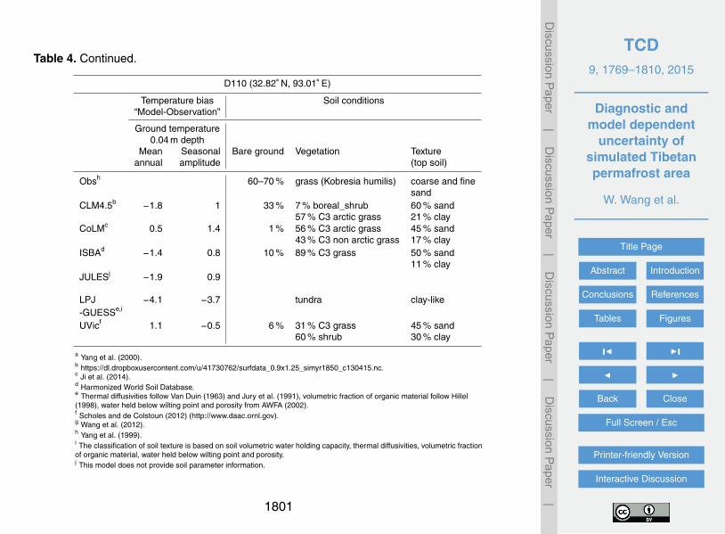
Table 4. Continued.

D110 (32.82◦ N, 93.01◦ E)

Temperature bias Soil conditions“Model-Observation”

Ground temperature0.04 m depth

Mean Seasonal Bare ground Vegetation Textureannual amplitude (top soil)

Obsh 60–70 % grass (Kobresia humilis) coarse and finesand

CLM4.5b −1.8 1 33 % 7 % boreal_shrub 60 % sand57 % C3 arctic grass 21 % clay

CoLMc 0.5 1.4 1 % 56 % C3 arctic grass 45 % sand43 % C3 non arctic grass 17 % clay

ISBAd −1.4 0.8 10 % 89 % C3 grass 50 % sand11 % clay

JULESj −1.9 0.9

LPJ −4.1 −3.7 tundra clay-like-GUESSe,i

UVicf 1.1 −0.5 6 % 31 % C3 grass 45 % sand60 % shrub 30 % clay

a Yang et al. (2000).b https://dl.dropboxusercontent.com/u/41730762/surfdata_0.9x1.25_simyr1850_c130415.nc.c Ji et al. (2014).d Harmonized World Soil Database.e Thermal diffusivities follow Van Duin (1963) and Jury et al. (1991), volumetric fraction of organic material follow Hillel(1998), water held below wilting point and porosity from AWFA (2002).f Scholes and de Colstoun (2012) (http://www.daac.ornl.gov).g Wang et al. (2012).h Yang et al. (1999).i The classification of soil texture is based on soil volumetric water holding capacity, thermal diffusivities, volumetric fractionof organic material, water held below wilting point and porosity.j This model does not provide soil parameter information.

1801





https://dl.dropboxusercontent.com/u/41730762/surfdata_0.9x1.25_simyr1850_c130415.nc

http://www.daac.ornl.gov

TCD9, 1769–1810, 2015



W. Wang et al.

Title Page



Tables Figures

J I

J I

Back Close

Full Screen / Esc



Discussion

Paper

|D

iscussionP

aper|

Discussion

Paper

|D

iscussionP

aper|

Table 5. Year-round relative model characteristics on TP.

Model Snow covera Albedob Soil waterc Unfrozen Organicwater effect layer

during phase insulationchange effect

CLM4.5 Medium Medium Medium yes YesCoLM Medium Medium Medium no NoISBA Low Low Medium yes YesJULES Low Low Medium yes NoLPJ-GUESS Medium Low High no NoUVic None Low High No No

a Low snow cover is confined to high elevations, medium tends to be on western TP.b LPJ-GUESS has constant albedo everywhere and UVic albedo varies slightly due to vegetation,year-round albedo variability for other models depends mainly on snow cover in winter and soil moisture,vegetation, etc in summer.c Soil water content includes both liquid and ice fractions.

1802





TCD9, 1769–1810, 2015



W. Wang et al.

Title Page



Tables Figures

J I

J I

Back Close

Full Screen / Esc



Discussion

Paper

|D

iscussionP

aper|

Discussion

Paper

|D

iscussionP

aper|

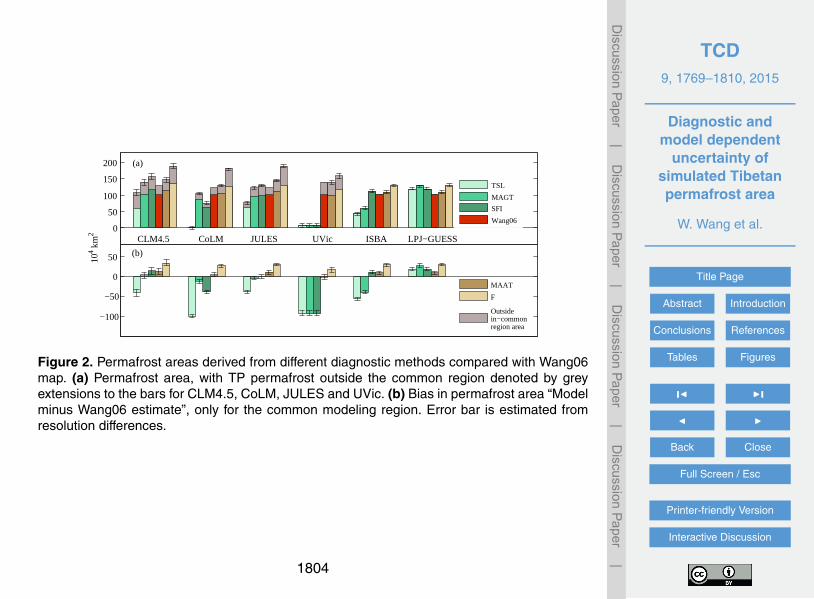
Figure 1. Permafrost maps derived from different diagnostic methods and models comparedwith Wang06 map. Permafrost inside the common modeling region is used for all-models inter-comparison, while permafrost outside allows further evaluation over the whole TP for CLM4.5,CoLM, JULES and UVic. The observation-based map of permafrost (Wang et al., 2006) isre-gridded to match model resolution.

1803





TCD9, 1769–1810, 2015



W. Wang et al.

Title Page



Tables Figures

J I

J I

Back Close

Full Screen / Esc



Discussion

Paper

|D

iscussionP

aper|

Discussion

Paper

|D

iscussionP

aper|

0

50

100

150

200

104 k

m2

−100

−50

0

50

TSL

MAGT

SFI

Wang06

MAAT

F

Outsidein−commonregion area

(b)

(a)

CLM4.5 CoLM LPJ−GUESSJULES UVic ISBA

Figure 2. Permafrost areas derived from different diagnostic methods compared with Wang06map. (a) Permafrost area, with TP permafrost outside the common region denoted by greyextensions to the bars for CLM4.5, CoLM, JULES and UVic. (b) Bias in permafrost area “Modelminus Wang06 estimate”, only for the common modeling region. Error bar is estimated fromresolution differences.

1804





TCD9, 1769–1810, 2015



W. Wang et al.

Title Page



Tables Figures

J I

J I

Back Close

Full Screen / Esc



Discussion

Paper

|D

iscussionP

aper|

Discussion

Paper

|D

iscussionP

aper|

UVic LPJ-GUESSCoLM

MAAT

MAGT

TSL

0.1

0.6

0.5

JULES

F

SFI0.2

CLM4.5ISBA

0.3

0.4

Figure 3. Kappa coefficient, K , quantifying the agreement between model-derived and Wang06maps (see Sect. 3.3). K ≥ 0.2 indicates at least fair agreement with Wang06 map. The lowertriangle is K for the whole TP and is only available for CLM4.5, CoLM, JULES and UVic, whilethe upper triangle is K for the common modeling region.

1805





TCD9, 1769–1810, 2015



W. Wang et al.

Title Page



Tables Figures

J I

J I

Back Close

Full Screen / Esc



Discussion

Paper

|D

iscussionP

aper|

Discussion

Paper

|D

iscussionP

aper|

Figure 4. Monthly soil temperature variations at 3 stations from models and observations.(a) and (c) soil temperature of top layer. (b) and (d) soil temperature of deeper layer, 1996–2000. “Mean” denotes annual average temperature.

1806





TCD9, 1769–1810, 2015



W. Wang et al.

Title Page



Tables Figures

J I

J I

Back Close

Full Screen / Esc



Discussion

Paper

|D

iscussionP

aper|

Discussion

Paper

|D

iscussionP

aper|

Figure 5. Monthly temperatures averaged over the selected western TP area in Fig. 1. (a) Forc-ing air temperature, (b) ground surface temperature, (c) 3 m soil temperature, averaged over1980–2000. “Mean” denotes annual average temperature.

1807





TCD9, 1769–1810, 2015



W. Wang et al.

Title Page



Tables Figures

J I

J I

Back Close

Full Screen / Esc



Discussion

Paper

|D

iscussionP

aper|

Discussion

Paper

|D

iscussionP

aper|

Figure 6. Winter snow depth for the common region, averaged over 1980–2000. Note thenonlinear color scale.

1808





TCD9, 1769–1810, 2015



W. Wang et al.

Title Page



Tables Figures

J I

J I

Back Close

Full Screen / Esc



Discussion

Paper

|D

iscussionP

aper|

Discussion

Paper

|D

iscussionP

aper|

Figure 7. Mean surface temperature offset: difference in mean winter temperatures betweensurface soil and air, averaged over 1980–2000. Warm colors indicate soil is warmer than airtemperature.

1809





TCD9, 1769–1810, 2015



W. Wang et al.

Title Page



Tables Figures

J I

J I

Back Close

Full Screen / Esc



Discussion

Paper

|D

iscussionP

aper|

Discussion

Paper

|D

iscussionP

aper|

Figure 8. Mean soil temperature offset: difference in mean winter temperatures between soilat 1 m depth and surface soil, averaged over 1980–2000. Warm colors indicate deep soil iswarmer than shallow soil.

1810





diagnostic and model dependent uncertainty of simulated

Documents