development towards a focus variation based micro … · development towards a focus variation...
TRANSCRIPT

Loughborough UniversityInstitutional Repository
Development towards afocus variation based
micro-co-ordinate measuringmachine
This item was submitted to Loughborough University's Institutional Repositoryby the/an author.
Additional Information:
• A Doctoral Thesis. Submitted in partial fulfilment of the requirementsfor the award of Doctor of Philosophy of Loughborough University.
Metadata Record: https://dspace.lboro.ac.uk/2134/14920
Publisher: c© Florine Hiersemenzel
Please cite the published version.

This item was submitted to Loughborough University as a PhD thesis by the author and is made available in the Institutional Repository
(https://dspace.lboro.ac.uk/) under the following Creative Commons Licence conditions.
For the full text of this licence, please go to: http://creativecommons.org/licenses/by-nc-nd/2.5/

Development towards a focus variation
based micro-co-ordinate measuring machine
by
Florine Hiersemenzel
A Doctoral Thesis submitted in fulfilment of the
requirements for the award of Doctor of Philosophy
of Loughborough University
May 2014

I | P a g e
Abstract The increasing number of small and fragile parts that are being manufactured using micro-
machining technology has raised the demand for co-ordinate measurement machines (CMM) that
can measure on a micro- and millimetric scale without contacting the part, thus avoiding damage to
the surface of the part. These instruments are expected to measure on a micro- and millimetric scale
with a measuring uncertainty in the nanometre range. A number of techniques used for contactless
surface measurements exist, such as the focus variation (FV) technique, which have the ability to
perform measurements on the micro- and millimetric scale in a short amount of time. These
instruments may have the potential to be implemented in a non-contact micro-CMM platform.
The FV technique is a relatively new addition to the wide range of techniques applied to metrology
instruments. It offers benefits, such as high aspect ratio measurements, over many competing
techniques but is yet unproven for its applicability for micro-CMMs. Industrial acceptance of FV
micro-CMMs will largely be determined by performance capability and the ability to traceably and
simultaneously robustly re-verify the instrument performance to a known set of international
standards. Developing a traceable route to the metre is not an easy feat and the first stage in doing
so is to determine the capabilities of FV instruments with respect to surface and geometric
measurement applications.
This thesis covers an investigation of the performance characteristics of the FV technique based on
an Alicona GmbH IFM G4, by assessing measurement noise, residual flatness, high aspect ratio
surface measurement quality and positional accuracy. These assessments, which have been
performed on a FV instrument, have not been previously published and are part of the novelty of
this research. Measurements of basic two dimensional and three dimensional shapes, such as
planes, cuboids and spheres, were performed in order to assess the FV technique’s suitability for
geometric measurements. These investigations form another part of the research novelty. The
outcome of these measurements indicated that spheres were well suited for this purpose.
Geometric measurements together with the investigations on measurement performances of the
IFM G4 form the groundwork for the exploration of the necessary changes to the IFM G4 to
transform it into a FV micro-CMM and the research for suitable acceptance, re-verification and
health check procedures.
The final part of the research was to develop a novel artefact suitable for the execution of the re-
verification and health check procedures, and demonstrate its applicability. Length measurements
using the novel re-verification artefact demonstrated the need for higher accuracy axes than

II | P a g e
currently used on a FV based surface texture instrument. The measurements also demonstrated that
a re-verification could be executed successfully with the novel artefact.
Key words: Focus variation, micro-CMM, performance characteristics, traceability, re-verification
artefact.

III | P a g e
Acknowledgements
I would like to express my deepest gratitude first and foremost to my first supervisor Dr Jon Petzing
for his guidance and unfailing support at any point throughout the project. Secondly, for their
supervision and guidance, I would like to offer my special thanks to Professor Richard Leach and Dr
Franz Helmli.
James Claverley and Claudiu Guisca from the NPL have given me the a lot of support for parts of the
experimental work, which was greatly appreciated, and I would like to thank Dr Reinhard Danzl and
Stephan Lehman from Alicona for their advice and assistance. My thanks also go to Professor Jeremy
Coupland. Of the technical staff at Loughborough University, I am particularly grateful for the
assistance given by Jagpal Singh and Trevor Atkinson.
I also appreciate the funding for this PhD project provided by Loughborough University, by the UK
National Measurement Office Engineering and Flow Metrology Programme (2011 – 2014) through
the National Physical Laboratory (NPL), and the company Alicona GmbH (Graz, Austria). This project
was also supported by the European Commission within the project “Minimizing Defects in Micro-
Manufacturing Applications (MIDEMMA) (FP7-2011-NMP-ICT-FoF-285614)”.
I would like to acknowledge the support by friends with whom I have enjoyed running, cycling,
kayaking and beach volleyball during these three years at Loughborough and those who have
encouraged me from a little further away. Most importantly, of course, I wish to thank my family for
their encouragement and support.

IV | P a g e
Publications
F. Hiersemenzel, J. Singh, J. N. Petzing, R. K. Leach, F. Helmli, R. Danzl. The assessment of residual
flatness errors in focus variation areal measuring instruments. 12th International Conference of the
European Society for Precision Engineering & Nanotechnology, Stockholm, Sweden, 231 – 234, June
2012. ISBN 978-0-9566790-0-0
F. Hiersemenzel, J. N. Petzing and R. K. Leach. Areal texture and angle measurements of tilted
surfaces using focus variation methods. 3rd International Conference on Surface Metrology, Annecy,
France, 85-89, March 2012. ISBN: 978-2-9536-1683-5
R. K. Leach, J. D. Claverley, F. Hiersemenzel, J. Petzing. Optical micro-coordinate metrology using the
focus variation technique. STC S (Surface), January 2013 Meeting CIRP – The International Academy
for Production Engineering, 24th January 2013.
F. Hiersemenzel, J. Singh, J.N. Petzing, J.D. Claverley, R.K. Leach, F. Helmli. Development of a
traceable verification route for optical micro CMMs. Accepted for presentation, 10th International
Conference on Laser Metrology, Machine Tool, CMM & Robotic Performance – Lamdamap 2013,
Kavli Royal Society International Centre, Buckinghamshire, UK, March 2013.
F. Hiersemenzel, J.D. Claverley, J.N. Petzing, F. Helmli, R.K. Leach. ISO compliant reference artefacts
for the verification of focus variation-based optical coordinate measuring machines. Accepted for
presentation, 13th International Conference of the European Society for Precision Engineering &
Nanotechnology, Berlin, Germany, May 2013.

V | P a g e
Contents
Abstract ................................................................................................................................ I
Acknowledgements............................................................................................................... III
Publications .......................................................................................................................... IV
Contents ............................................................................................................................... V
Glossary and key technical terms ........................................................................................... XI
Chapter 1: Introduction to the research
1.1 Introduction .................................................................................................................. 1
1.2 Research objectives ....................................................................................................... 3
1.3 Structure of the thesis ................................................................................................... 4
Chapter 2: Literature review
2.1 A brief story about the metre ...................................................................................... 6
2.2 Co-ordinate metrology .................................................................................................. 7
2.2.1 The story of co-ordinate metrology ............................................................. 7
2.2.2 The story of CMMs ........................................................................................ 8
2.2.3 Key technical terms ....................................................................................... 12
2.2.4 Review of micro-CMMs and micro-probes .................................................. 14
2.2.4.1 Two philosophies for the development of micro-CMMs .............. 14
2.2.4.2 Miniature tactile CMMs ................................................................ 15
2.2.4.3 Miniature tactile probes: static micro-probes .............................. 17
2.2.4.4 Small-scale resonant type micro-probes ...................................... 20
2.2.4.5 Opto-tactile probing systems........................................................ 21
2.2.4.6 X-ray computed tomography technique applied to micro-CMMs 22
2.2.5.7 Micro-probes made with the ‘bottom-up’ philosophy: scanning
probe microscopy ..................................................................................... 23
2.2.4.8 Micro-probes made with the ‘bottom-up’ philosophy: optical
microscopy ................................................................................................ 24
2.2.4.9 Micro-probes in summary ............................................................ 25
2.3 Surface metrology ......................................................................................................... 27
2.3.1 The story of surface metrology ..................................................................... 27
2.3.2 Techniques used for surface measuring instruments ................................... 30

VI | P a g e
2.3.3 Calibration artefact for optical surface texture measuring instruments ..... 31
2.4 Re-verification of CMMs ............................................................................................... 32
2.4.1 Introduction .................................................................................................. 32
2.4.2 Calibration, acceptance, re-verification and health-check tests for CMMs . 34
2.4.3 Environmental considerations ..................................................................... 36
2.4.4 Review of re-verification artefacts for micro-CMMs .................................... 37
2.4.4.1 Ball Plates and 2D artefacts .......................................................... 37
2.4.4.2 Task specific artefacts ................................................................... 43
2.4.4.3 Other artefacts .............................................................................. 46
2.5 Summary ....................................................................................................................... 48
Chapter 3: Focus variation
3.1 Introduction to focus variation ..................................................................................... 49
3.2 Development of the shape from focus technique ........................................................ 50
3.3 FV instrument: hardware .............................................................................................. 57
3.4 FV Instrument: software ............................................................................................... 60
3.5 Limitations of the FV technique: data dropout and re-entrant features ..................... 62
3.6 Measurement settings of FV instruments .................................................................... 67
3.6.1 Illumination ................................................................................................... 68
3.6.2 Polariser ........................................................................................................ 69
3.6.3 Contrast ......................................................................................................... 70
3.6.4 Lateral and vertical resolutions ..................................................................... 70
3.6.5 Objective Lenses ........................................................................................... 72
3.7 Summary ...................................................................................................................... 76
Chapter 4: Instrument performance characteristics: measurement noise
4.1 Introduction .................................................................................................................. 78
4.2 Calculating measurement noise.................................................................................... 79
4.2.1 Subtraction method ...................................................................................... 80
4.2.2 Addition method .......................................................................................... 80
4.3 Assessing measurement noise of the IFM G4 ............................................................... 81
4.3.1 Method of assessing the effect of settings on noise ..................................... 81
4.3.2 Results and discussion ................................................................................. 88
4.3.2.1 Reference values ........................................................................... 88
VII | P a g e
4.3.2.2 Setting induced measurement noise for each lens ...................... 89
4.3.2.3 Results organised by setting ......................................................... 92
4.3.2.4 Results across all lenses ................................................................ 95
4.3.3 Discussion and conclusions ........................................................................... 96
Chapter 5: Instrument performance characteristics: residual flatness
5.1 Introduction .................................................................................................................. 99
5.2 Measuring residual flatness of areal surface texture measuring instruments ............. 100
5.3 Measuring residual flatness of a FV instrument ........................................................... 101
5.3.1 Ten image method ........................................................................................ 102
5.3.2 Ten image with filter method ....................................................................... 104
5.3.3 Hundred image method ................................................................................ 104
5.3.4 Experimental results .................................................................................... 104
5.3.5 Conclusions and discussion ........................................................................... 111
5.4 Residual flatness in the context co-ordinate measurements ...................................... 113
Chapter 6: High aspect ratio surface measurements
6.1 Introduction .................................................................................................................. 117
6.2 Methods and results ..................................................................................................... 119
6.2.1 Surface parameters for high aspect ratio measurements ............................ 119
6.2.2 Instrumentation ............................................................................................ 120
6.2.3 Large surface roughness measurements ...................................................... 121
6.2.4 Effects of settings: illumination .................................................................... 122
6.2.5 Effects of settings: polariser .......................................................................... 124
6.2.6 Effects of settings: lateral resolution compensation .................................... 126
6.2.7 The effect of different surface roughness ..................................................... 127
6.2.8 The effect of profile length on Ra and of λc on Sq ........................................ 129
6.2.8.1 Ra-parameters............................................................................... 129
6.2.8.2 Sq-parameters ............................................................................... 131
6.2.9 Comparison between the IFM G4 and the PGI ............................................ 132
6.3 Discussion and conclusions .......................................................................................... 133
Chapter 7: Geometric measurements using FV
7.1 Introduction .................................................................................................................. 137
7.2 Geometric angle measurements................................................................................... 137

VIII | P a g e
7.2.1 Introduction .................................................................................................. 137
7.2.2 Assessing the variation of angle measurements .......................................... 136
7.2.3 Results ........................................................................................................... 138
7.2.4 Conclusions ................................................................................................... 140
7.3 Length measurement error assessment using gauge blocks ........................................ 141
7.3.1 Introduction .................................................................................................. 141
7.3.2 Methods for gauge block measurements .................................................... 141
7.3.2.1 Configuration 1: wrung gauge blocks ............................................ 143
7.3.2.2 Configuration 2: staggered gauge blocks ...................................... 145
7.3.2.3 Configuration 3: non-wrung gauge blocks .................................... 145
7.3.3 Results .......................................................................................................... 146
7.3.3.1 Configuration 1: wrung gauge blocks ............................................ 146
7.3.3.2 Configuration 2: staggered gauge blocks ...................................... 147
7.3.3.3 Configuration 3: non-wrung gauge blocks .................................... 149
7.3.4 Conclusions and discussion ........................................................................... 150
7.4 Spheres.......................................................................................................................... 152
7.4.1 Introduction .................................................................................................. 152
7.4.2 Measurements of spheres ............................................................................ 152
7.4.2.1 Comparison of different sphere materials .................................... 155
7.4.2.2 Etching ruby spheres ..................................................................... 155
7.4.2.3 Etching zirconia spheres ................................................................ 156
7.4.2.4 Using differently sized spheres ..................................................... 157
7.4.2.5 Single FoV versus multiple FoV ..................................................... 158
7.4.2.6 Variation of measurements .......................................................... 158
7.4.3 Results of sphere measurements ................................................................. 160
7.4.3.1 Comparison of different sphere materials ................................... 160
7.4.3.2 Etching ruby spheres ..................................................................... 162
7.4.3.3 Etching zirconia spheres ................................................................ 164
7.4.3.4 Using differently sized zirconia spheres ........................................ 171
7.4.3.5 Single FoV versus multiple FoVs .................................................... 175
7.4.3.6 Variation of measurements ........................................................... 178
7.4.4 Discussion and conclusions ........................................................................... 179
7.5 Summary ....................................................................................................................... 181

IX | P a g e
Chapter 8: FV as a new technique for optical micro-CMMs
8.1 Introduction .................................................................................................................. 184
8.2 Suitability of FV technique for optical micro-CMMs ..................................................... 181
8.2.1 Hardware ...................................................................................................... 185
8.2.1.1 Structural design ........................................................................... 185
8.2.1.2 Measurement system ................................................................... 187
8.2.2 Positional accuracy ....................................................................................... 190
8.2.2.1 Introduction .................................................................................. 190
8.2.2.2 Method of positional accuracy assessment of the IFM G4 ........... 192
8.2.2.3 Results: accuracy and repeatability of positioning ....................... 194
8.2.2.4 Discussion and conclusions ........................................................... 196
8.2.3 Software ....................................................................................................... 197
8.3 Acceptance, re-verification and health check tests for FV CMMs ................................ 199
8.3.1 Acceptance and re-verification for CMMs .................................................... 200
8.3.2 ISO 10360-8: acceptance and re-verification for CMMs with optical distance
sensors ................................................................................................................... 201
8.3.3 Health checks for CMMs with optical distance sensors ............................... 203
8.3.4 ISO 10360-8: potentials and restrictions for FV micro-CMMs ...................... 204
8.3.4.1 Measurements for probe form error and probe size error .......... 204
8.3.4.2 Length measurement error........................................................... 205
8.3.4.3 Health check ................................................................................. 207
8.4 Summary ...................................................................................................................... 207
Chapter 9: Novel re-verification artefact
9.1 Introduction .................................................................................................................. 209
9.2 Artefact specification .................................................................................................... 209
9.3 First concept of a re-verification artefact for FV micro-CMMs ..................................... 214
9.4 Artefact number two .................................................................................................... 217
9.5 Artefact design: mission Fritz ........................................................................................ 219
9.6 Size error measurements using Artefact Fritz .............................................................. 226
9.6.1 Method ......................................................................................................... 226
9.6.2 Results ........................................................................................................... 227
9.6.2.1 Calibration of Artefact Fritz ........................................................... 227
9.6.2.2 Application of Artefact Fritz to the IFM G4 ................................... 229

X | P a g e
9.6.3 Conclusions.................................................................................................... 239
9.7 Summary ....................................................................................................................... 241
Chapter 10: Conclusions and further work
10.1 Conclusions ................................................................................................................. 246
10.2 Future work ................................................................................................................. 254
10.3 A last note on the topic of machines .......................................................................... 257
Chapter 11: References ......................................................................................................... 259

XI | P a g e
Glossary and key technical terms
AFM: atomic force microscope
Aspect ratio of a surface: inclination of a surface
BIMP: Bureau International des Poids et Mesures
BS: British Standard
CCD: charge-coupled device
CGPM: Conférence Général des Poids et Mesures
CMM: co-ordinate measuring machine
CSI: confocal scanning interferometer
DEA: Digital Engineering Automation
FV: focus variation
GmbH: Gesellschaft mit beschraenkter Haftung
GPS: global positioning satellite system
HC: high contrast
HExp: high exposure time
HF: hydro-fluoric
High aspect ratio: 55 degrees to 70 degrees
HLRes: high lateral resolution (low value)
HVRes: high vertical resolution (low value)
IFM: Infinite Focus Microscope
ISO: International Organisation for Standardisation
LC: low contrast
LExp: low exposure time
LLRes: low lateral resolution (high value)
Low aspect ratio: 0 degrees to 40 degrees
LR: lateral resolution
LVRes: low vertical resolution (high value)
Medium aspect ratio: 40 degrees to 55 degrees
NA: numerical aperture
NIST: National Institute of Standards and Technology, US
NPL: National Physical Laboratory, UK
NTB: Interstaatlische Hochschule fuer Technik Buchs
PCD: pitch circle diameter

XII | P a g e
PSI: phase shifting interferometry
PTB: Physikalisch Technische Bundesanstallt
R: reference
SPM: scanning probe microscopy
TTH: Taylor Taylor Hobson
Very high aspect ratio: 70 degrees to 80 degrees
VDI: Verband deutscher Ingenieure
VR: vertical resolution
VS: ‘vibroscanning’
2D: two dimensional
2½D: two and a half dimensional
3D: three dimensional
Key technical terms
Metrology, like many other fields of research, has its own set of technical terms. Defined below are
some of the most important technical terms used frequently in this thesis. The definitions were
taken from the following standards: BS 5233, 1986; BS 7172, 1989; BS ISO 3534-1, 1993; BS ISO
3534-1, 1993; ISO 129, 2004; and BSI PD 6461-1, 1995.
Measurand: “A quantity subjected to measurement”;
Workpiece: “The object or component under test, containing the geometric feature being assessed”;
Accuracy: “The closeness of agreement between a test result and the accepted reference value”;
Precision: “The closeness of agreement between independent test results obtained under stipulated
conditions”;
Trueness: “The closeness of agreement between the average value obtained from a large series of
test results and an accepted reference value”;
Repeatability: “Precision under repeated conditions”;
Reproducibility: “Precision under reproducibility conditions”;
(Standard) uncertainty: “An estimate attached to a test result which characterizes the range of
values within which the true value is asserted to lie”; mathematically, the uncertainty can be defined
differently. In this context the uncertainty was always defined by the standard deviation for which
the formula is as follows.
𝜎 = �1𝑁∑ (𝑥𝑛 − µ)2𝑁𝑛=1 , where xi is the measured value and μ is the mean of all N samples.

XIII | P a g e
Expanded uncertainty and coverage factor (k): “The expanded uncertainty is the result of
multiplying the standard uncertainty by a factor (usually 2 or 3), which is referred to as the coverage
factor”.
Error of measurement: “The result of the measurement minus the true value of the measurand”;
Deviation: “Value minus its reference value”;
Tolerance: “The maximum error that is to be expected in some value; maximum deviation of a
manufactured component from some specified value”;
Resolution: the specification of how finely the output scale is divided into subdivisions; “A quantitive
expression of the ability of an indicating device to distinguish meaningfully between closely adjacent
values of the quantity indicated”;
Measurement span: “a range bracketed by the minimum and maximum values of a quantity that the
instrument is designed to measure”.

1 | P a g e
Chapter 1: Introduction to the research
1.1 Introduction
The research reported in this thesis is in the field of metrology, in the context of measurement
requirements for the manufacturing of small parts. The importance of metrology is sometimes not
recognised, and as a result, parts are manufactured with a poor quality and have a shorter life time.
The poem “one-hoss shay” pictures an example, which emphasises the importance of precision
engineering, of which metrology is an essential part.
One-hoss shay
By Oliver Wendell Holms
…. Of the wonderful one-hoss shay,
That was built in such a logical way
It ran a hundred years to a day
And then….
How it went to pieces all at once, -
All at once, and nothing first, -
Just as bubbles do when they burst.
Now in the buildings of chaises, I tell you what,
There is always somewhere a weakest spot, -
In hub, tyre, felloe, in spring or thill,
In panel, or crossbar, or floor, or sill,
In screw, bolt, thoroubrace – lurking still
Find it somewhere you must and will, -
Above or below, or within or without, -
And that’s the reason, beyond a doubt,
A chaise breaks down, but doesn’t wear out.
This is an extract from the poem “One-hoss shay” by Oliver Wendell Holms (Holms, 1858). The poem
describes how the deacon’s one-hoss (horse) shay wears out, and in comparison how an ordinary
chaise breaks down because it has not been built in a logical way as with the one-hoss shay. The
logical build of the one-hoss shay implies that the manufacturing of every part was very good. But

2 | P a g e
how can the quality of each part be assessed? This is where metrology enters the manufacturing
cycle of a part; inspection of parts can lead to improved quality and thus to longer lasting products
that do not break down but wear out.
Metrology has many different subcategories but the subcategories of interest here are co-ordinate
metrology, which is the knowledge of the dimensional properties of a workpiece (e.g.: angles,
diameters, lengths), and surface metrology, which is the measurement of surface characteristics
such as roughness and waviness. The tools for co-ordinate and surface metrology are co-ordinate
measuring machines (CMM) and surface topography measuring instruments, respectively. A typical
CMM with a measuring volume of one cubic metre can measure with uncertainties on the scale of a
few micrometres, whilst surface texture measuring instruments are capable of performing
measurements with uncertainties on the nanometric scale.
New micro- and nanotechnologies used for manufacturing allow the production of smaller and
smaller parts with decreasing manufacturing tolerances. Examples for such parts are micro-gears,
semi-conductors, micro-holes or micro-machined biomedical parts, as shown in Figure 1.1, (Cowley,
2011). Traditional CMMs cannot perform the measurements of such small parts with the required
maximum measurement error, and in some cases cannot perform such measurements at all because
of the probing sphere size. Consequently the demand for micro-CMMs capable of measuring small
parts (on the millimetric scale) with small measuring uncertainty (on the nanometric scale) is
increasing. The demand for new instruments permits instrument manufacturers to make
instruments that are task-specific. The alternative to task-specific instruments are instruments that
have the capability to measure a wide spectrum of parts. Both approaches to designing micro-CMMs
have their advantages and disadvantages.
Figure 1.1: Micro-machined biomedical components (Cowley, 2011)

3 | P a g e
One route to designing contact micro-CMMs is by miniaturising existing large-scale CMMs, however,
physical limits are met, such as the snap-in effect where the contact probe is drawn to the surface by
the surface forces. Techniques such as vibrating probes have been implemented in CMM-platforms
in order to overcome these physical limits (Claverley and Leach, 2013). Contact micro-CMMs also
have the disadvantage of long measurement times and are expensive (approximately £200k –
£250k). These contact micro-CMMs are designed to operate in temperature (20 °C ± 0.5 °C) and
humidity (50 % ± 10 % rH) controlled clean rooms, which are expensive to establish and run.
Non-contact micro-CMMs have the advantage that the object’s surface is not damaged during the
measuring process and the physical limitations of contact transducers do not apply. Optical areal
techniques have the advantage of measuring a large amount of data within a short period of time
(Leach, 2011). The focus variation (FV) technique is an optical areal technique that is currently only
implemented in surface measurement instruments, some of which have capabilities that extend to
surface form measurements. FV instruments provide a flexible and traceable XYZ measurement
capability and this is the reason for investigating the FV technique with regard to co-ordinate
metrology.
The choice for implementing the FV technology into a CMM system is primarily because of its ability
to measure high aspect ratio surfaces more reliably than other optical techniques. However, further
characteristics of the FV technology have to be investigated with regard to dimensional
measurements, in order to give information on performance characteristics of the FV technique in
terms of surface texture and dimensional measurements. Furthermore, any acceptance and re-
verification procedure requires an appropriate calibrated artefact, and although many calibrated
artefacts exist, they are typically instrument specific. Consequently, the relevancy of existing surface
texture and co-ordinate artefacts require investigation with the possibility that a specific artefact
would need to be designed.
1.2 Research objectives
The objectives of this research are to:
• Investigate applications to justify the implementation of a new technique as a micro-CMM
platform that can offer advantages over other techniques currently used for micro-CMMs.
• Understand how the FV technique works; its drawbacks and advantages over other areal
optical instruments.

4 | P a g e
• Explore methods of assessing performance characteristics in terms of measurement noise
and residual flatness, and simultaneously to explore the influence of instrument settings on
these performance characteristics.
• Explore the performance characteristics of the FV technique for high aspect ratio surface
measurements as this is one of the key advantages that this technique has over other optical
techniques.
• Assess the capability of the FV technique positional accuracy with the view to using this
instrument as a micro-CMM.
• Assess the capability of the FV technique to perform basic geometric measurements.
• Explore a traceable route to link the FV technique performance with the definition of the
metre, in the context of co-ordinate measurement (i.e. acceptance, re-verification and
health check tests).
• Identify a suitable re-verification artefact, which can also serve the purpose of health
checking, for a future FV technique based micro-CMM.
1.3 Structure of the thesis
This thesis comprises of nine chapters, which present the background to the research and the novel
content of the research.
Chapter 1 is an introduction that presents the context of the research, the motivation, the aims and
the structure of the thesis.
Chapter 2 presents a literature review on the history, the instruments and measurement techniques
used for dimensional and surface texture metrology. The survey also gives an overview of the
calibrated artefacts that are used to assess the performance of areal optical surface texture
measuring instruments and micro-CMMs.
Chapter 3 is also part of the literature review, on which this research builds up. The chapter is
concerned with all aspects of the FV technique: the history, the theory, the development, the
applications, and the benefits and drawbacks of FV instruments.
Chapter 4 to 6 develops an understanding of the performance characteristics of the FV technique.
The instrument, on which the research is based, is the Infinite Focus Microscope (IFM G4)
manufactured by the Austrian company Alicona GmbH. The investigation for assessing the suitability
of a FV surface texture measuring instrument as a platform for a FV micro-CMM includes the

5 | P a g e
assessment of measurement noise (Chapter 4), residual flatness (Chapter 5), and high aspect ratio
measurements (Chapter 6).
Chapter 7 presents experiments where the IFM G4 is used for certain geometric measurements.
Three investigations are presented; the measurement of angle of a surface with respect to the
horizontal plane of the instrument's co-ordinate system, distance measurements using gauge blocks,
and sphere measurements.
Chapter 8 focuses on the suitability of the FV technique for co-ordinate measurement applications,
on the instrument’s positional accuracy, and on an acceptance and re-verification procedures for FV
micro-CMMs. Furthermore, existing standards and artefacts are assessed for suitability and it is
investigated what tasks a FV micro-CMM should have to complete in order to assess the instrument
performance. Similarly, a health check procedure for FV micro-CMMs is investigated.
Chapter 9 presents the development process and the performance of a novel re-verification artefact.
As a result of numerous techniques that have been implemented in CMMs with various measuring
volumes, a number of re-verification artefacts exist. However, all re-verification artefacts for micro-
CMMs are not suitable to be measured by the FV technique due to either the lack of nano-scale
roughness on the surfaces or the unsuitable shape and dimensions of the artefact. Therefore, a
novel re-verification artefact is designed.
Chapter 10 is a summary of all conclusions drawn from the previous chapters and suggests work that
could be done to extend this research further. Chapter 11 is a list of the works that have been used
as sources of information for this research.
In summary, the anticipated novel outcomes of the research reported here in the thesis will be as
follows:
• Identify a method for the assessment of measurement noise.
• Understanding of the influence of settings on measurement noise.
• Development of a method for the assessment of residual flatness.
• Understanding of performance characteristics of high aspect ratio measurements.
• Understanding of the suitability of the FV technique for geometric measurements.
• Development of a re-verification procedure for a FV technique based micro-CMM, and
• An artefact suitable for a traceable re-verification of a FV technique based micro-CMM.

6 | P a g e
Chapter 2: Literature review
2.1 A brief story of the metre
The definition of the metre is based on the speed of light: it is the length of the path that light travels
in vacuum in the time duration of 1/c seconds, c being the speed of light (299,792,458 m/s). This is
the latest definition of the metre that was officially adopted in 1983 by the intergovernmental treaty
organisation Conférence Générale des Poids et Mesures (CGPM) (NIST, 2000).
The history of the metre dates back to the 18th century, when it was decided by the French that a
well-defined measure of length was necessary. Prior to the metre, measures of length generally
corresponded to measures of parts of the human body (i.e. foot, ell, yard) and these measures could
vary from one village to another or from person to person (NPL, 2010).
In 1791, the French Academy of Sciences (Académie des Sciences) decided that the metre should be
traced to a quarter of the Earth’s circumference: the metre was to be one ten-millionth of the
quarter of the length meridian through Paris from the North Pole to the equator (NIST, 2000). For six
years, Pierre Mechain and Jean-Baptiste Delambre measured the length from Dunkirk through Paris
to Barcelona. The irregular shape of the earth (as well as occasional imprisonments) posed problems
for the scientists when measuring and calculating the metre, and caused an error of 0.2 m in their
final result. Despite the error, this length was made a standard and solid artefacts were made. The
first platinum-iridium alloy artefact was cast in 1874, which adopted the name ‘1874 Alloy’. In 1889,
a new artefact of the same alloy was made but with better defined percentage of iridium content
(10 % ± 0.0001 %), which was to be measured at 0 ̊C, which was kept in atmospheric pressure in
Paris at the Bureau International des Poids et Mesures (BIPM) (NIST, 2000).
The 1889 definition of the metre and the associated artefacts were dismissed by the CGPM in 1960
and replaced by a new definition of the metre, which traced the metre to the wavelength of
krypton-86 radiation. The redefinition of the metre narrowed the uncertainty associated with the
realisation (manufacture and verification) of the metre by using optical interferometry (BIPM, 2006).
Only 13 years after the redefinition, a new definition of the metre was announced in 1983 by the
CGPM. This definition, which makes the metre traceable to the second, is the standard to date, and
is as follows.
“The length of the path travelled by light in a vacuum
during a time interval of 1/299 792 458 of a second” (NPL, 2010).

7 | P a g e
2.2 Co-ordinate metrology
2.2.1 The story of co-ordinate metrology
During the time when the ell and similar non-metric measures of length were still the norm for
metrology, the science of measurement, the entire manufacturing process of multi-piece objects
was usually made in one location. This set-up permitted correction, without much delay, of errors
when the assembly of the pieces failed because the tools were at hand. The tolerances on the
manufactured items were not as tight as they are today and the time-factor was not as important.
The first types of co-ordinate measuring instruments were used predominantly in the area of civil
engineering and navigation (Schwenke et al., 2002). The “Jacob bar” is an example of an instrument
used around the 14th century by civil engineers and navigators to take optical bearings using
triangulation. When more accurate manufacturing results were needed, primitive manual measuring
instruments such as rulers with their own respective measuring units were used. Later, the
introduction of a defined length with international relevancy was important for the development of
precision manufacturing, which inevitably links with precision metrology. Gauge blocks, callipers and
micrometers could be made with metric scales and high accuracies. Table 2.1 lists manual measuring
devices commonly used before the co-ordinate measuring machine (CMM) revolutionized precision
engineering in mass-production industries.
In the first half of the 20th century industrialisation required replacement of manual measuring
instruments by more sophisticated devices. Large factories were built, many workers employed and
items came off the manufacturing line at a higher frequency. Workers became specialised, the
manufacturing tolerances became tighter and the time-factor more important. The ability to amend
items was lost in the movement towards mass-production and items were scrapped. In order to
obtain a high percentage of well-manufactured items, regular inspections had to be built in the
production line. The outcomes of the inspections reflected the manufacturing precision of the
machines used for the process. Inspections had to be completed rapidly and this called for
automated measuring devices.
Gradually technology caught up with the demands of the industry, and in 1952, the first computer
numerically controlled CMM was built by Digital Engineering Automation (Wenzel, 2009). Computer
numerical control units are now common for metrology. Today, manufacturing lines exist with built-
in automatic inspection systems. A number of companies, such as Renishaw and Zeiss, produce

8 | P a g e
CMMs based on a variety of different techniques. Multi-sensor CMMs also exist, which aim for a
broader range of application (Wenzel, 2009).
The story of coordinate metrology - the field of knowledge concerned with dimensional
measurements (BS5233, 1986) – did not only start with the introduction of CMMs but long before
that, in the times when the rule was the principal measuring instrument. Coordinate metrology has
always been used to assess the deviations of a workpiece from its intended shape, which today is
from the shape usually specified on the technical drawings (Whitehouse, 2003), and which comprise
dimensions such as lengths, roundness, straightness, flatness and cylindricity, with their respective
tolerances.
Table 2.1: Manual measuring instruments and their purpose (Mitutoyo, 2010)
Measuring instrument Measurable features
Rule/ tape measure Length
External micrometer Outer diameters, thickness, root
diameter, thread diameters, etc.
Internal micrometer Diameters: Square and round grooves,
spline, serration, threaded hole
Callipers (Vernier/dial) Length, hole diameter
Vernier height gauge Height
Dial test indicator Height deviation
Cable length measuring
device (wheel) Length
Gauge blocks Length
Angle gauges Angle
2.2.2 The story of CMMs
The CMM found its origin in the period of time when, on the advancing assembly lines, cars had to
be manufactured with high accuracy. Interchangeable parts had to be measured in a short period of
time. The reason for the development of the CMM at that time was not primarily accuracy but time-
efficiency. Prior to the introduction of CMMs, measurements had to be carried out using gauge
blocks and functional gauges (such as callipers), each of which had to be calibrated carefully thereby
taking a lot of time. In the production line, a measurement of dimensions enhances the
manufacturing quality of a product; however, the additional process slows down the overall

9 | P a g e
production speed, therefore, costing time and money. Gauge blocks and functional gauges could no
longer meet the manufacture’s expectations and since then they have been used mainly for the
calibration of CMMs, which are used to fulfil these growing requirements (Bosch, 1995).
Two companies claim the invention of the CMM in the 1950s: Ferranti Metrology, and Digital
Engineering Automation (DEA). Ferranti Metrology (now International Metrology Systems) in
Scotland was the first company to develop a CMM with a cantilever design and a fixed probe. The
machine - at the time referred to as the ‘XYZ Machine’ - had a simple digital read out and was based
on digital command control (Wenzel, 2009). The Italian company DEA, which has become part of
Hexagon Metrology, was the first company to produce a portal frame CMM with a hard probe,
based on computer numerical control, and to refer to it as a ‘C.M.M.’ called ‘Alpha’.
Shortly after Ferranti Metrology and DEA introduced the first CMMs, other companies from around
the world started manufacturing CMMs and the market became very competitive and diverse. The
British company LK Tool introduced the first bridge type CMM, which has become the most standard
type of CMM structure (Wenzel, 2009). Many other types of structures were applied to CMMs,
commonly used configurations being the cantilever, gantry, horizontal arm, moving table, fixed
bridge and articulated arm.
The tactile touch trigger sensing system was used to make the first automated CMM in the mid-
1970s. The development of touch trigger sensors led to the establishment of the company Renishaw
which claims to have become the world leading company for the supply of CMM measuring heads
(Harding, 2013). Since the introduction of tactile touch trigger probes a variety of technologies have
been applied to CMM probes and in some CMMs, two or more sensing technologies are embedded,
in order to give the machine a broad application capability. Recent years have also seen the
introduction of 5-axis (three translational and two rotational) measuring technology thus widening
the capability of the traditional CMM.
As a result of the large variety of applied sensor technologies and structural types (and consequently
their measuring capabilities) CMMs can be found with various combinations of accuracy, precision,
size and measurement volume. In the strict sense of the definition of the CMM, which are those
machines that give physical representations of a 3D rectilinear Cartesian co-ordinate system (Bosch,
1995), the American global positioning satellite systems (GPS) and the Russian GLONAS are included.
The GPS and GLONAS networks may be the largest coordinate measuring systems but they are not
directly used in manufacturing industry and will not be considered further in this context. However,
some companies have made positioning systems that can be used indoors and for a very large

10 | P a g e
measuring scale, such as the iGPS by Nikon Metrology. Other technologies used for very large
manufacturing volumes, such as required in the aerospace industry, are laser trackers, which have a
high level of precision and a good reliability, and photogammetry systems (Harding, 2013).
Up until the 1980s, traditional CMMs were kept in temperature controlled environments (20 ̊C)
because the instruments were affected too strongly by temperature fluctuations. Therefore,
workpieces had to be transported from the production line to the metrology room to be measured.
Portable measuring machines, which were introduced in the 1980s, allowed part inspections to be
completed by the production line, thus saving time at the cost of accuracy.
The construction of traditional CMMs has been refined over the years with the help of improving
technology (e.g. linear measurement glass scales) or the research of materials (e.g. lighter and stiffer
alloys) and as a result measurements can be accomplished with increasingly finer resolutions and
smaller uncertainty. Now traditionally structured CMMs can achieve accuracies of just a few
micrometres. Currently some companies are investing in the research of micro-CMMs with the aim
to push the boundaries of part dimensions and machine uncertainty and accuracy, and thus to adapt
to the field of nanotechnology.
The development of computers and computational power had a direct influence on the inspection
and control software of CMMs. Whilst in the early stages of CMMs, the manufacturing companies
provided the inspection software, today separate companies or subsidiaries, such as PC-DMIS, exist
that are primarily concerned with dimensional measurement inspection software (Harding, 2013).
Today, CMM software is advanced and many features can be measured and relationships calculated.
Measurable features can be divided into two classes: single features and related features. Single
features can have form errors such as straightness and flatness. Related features can have
orientation (e.g. parallelism), location (e.g. symmetry) and run-out errors. Attaching tolerances to
each type of error applicable to a workpiece allows for a go/no-go decision after the workpiece’s
measurement. Figure 2.1 shows the classification of all tolerances that can constrain the
manufacture of any workpiece. Not all co-ordinate measuring instruments have the same measuring
capabilities. Some instruments are specific to one particular measurement, for example the Talyrond
by Taylor Hobson designed to measure roundness, and other measuring instruments are designed to
have a broad application range, such as the traditional tactile CMM. Table 2.2 lists common types of
co-ordinate measuring instruments and the features, which the instruments are capable of
measuring.

11 | P a g e
Figure 2.1: Measurable characteristics of a workpiece in co-ordinate metrology (ISO 1101, 2012)

12 | P a g e
Table 2.2: Measuring capabilities of CMMs
Measuring instrument Measurable features
Traditional tactile CMMs Lengths dimensions, angles, cylindricity, circularity, flatness,
parallelism, straightness, roundness, squareness, concentricity,
symmetry, perpendicularity, angularity, circular and total run-out.
Roundness measuring
instruments
Roundness/ circularity, profile of any line.
Theodolites (modern) Angles.
Laser projection systems Length dimensions, circularity, parallelism, straightness, roundness,
squareness, concentricity, symmetry, perpendicularity, angularity,
circular and total run-out, angles.
Laser trackers Position, straightness.
Laser radar Length dimensions.
Photogrammetry/
videogrammetry systems
Length dimensions, cylindricity, circularity, flatness, parallelism,
straightness, roundness, squareness, concentricity, symmetry,
perpendicularity, angularity, circular and total run-out, angles.
Scanning devices Length dimensions, cylindricity, circularity, flatness, parallelism,
straightness, roundness, squareness, profile of any line, profile of a
surface, concentricity, symmetry, perpendicularity, angularity, circular
and total run-out, angles.
Articulating arms Length dimensions, cylindricity, circularity, flatness, parallelism,
straightness, roundness, squareness, concentricity, symmetry,
perpendicularity, angularity, circular and total run-out, angles.
GPS/ GLONAS/ iGPS Position, distance.
2.2.3 Techniques implemented in CMMs
The technologies implemented in CMMs that are used in industry for inspection purposes can be
split into two groups: touch trigger sensors and measuring systems. The characteristic of touch
trigger sensors is the go/no-go (binary) information transmission: the output is detected when it
passes a discrimination threshold, which is the minimum level of output needed to make the
magnitude detectable (BS 5233, 1986). For example, a touch trigger probe is flexible in all directions,
so for a measurement (the position of the object’s surface) to be registered, the force applied on the
probe has to surpass a threshold force (Coleman, 1997). Similarly, touch trigger sensors based on

13 | P a g e
optical technology either register or do not register a surface thus making point measurements. An
example for an optical touch trigger sensor is a touch probe with mirrors rigidly attached to the top
of the stylus, which are moved when the stylus comes into contact with a surface (Haitjema, 2001).
Beams of light are reflected by mirrors that are mounted to the top of the stylus and thus are
influenced by the movement of the stylus. A measurement is triggered when a certain reflection
angle is bypassed.
In contrast to point measurement systems (touch trigger sensors), measuring sensors have a
continuous change in output, for example optical systems based on photogrammetry or optical
tactile systems. Touch trigger sensors as well as measuring sensors can make use of optical and
tactile technologies, only x-ray computed tomography is unique to measuring sensors. Measuring
sensors are more diverse in terms of applied technologies: there are especially many different types
of optical sensors, which are based on for example interferometry, image processing and
triangulation. X-ray computer tomography measuring techniques are relatively new to CMMs.
Currently research projects are concerned with computed tomography as a new technique for
CMMs on both a large (1 m) and small (up to 100 mm) scale (Nash, 2013). Figure 2.2 shows the
technologies used for touch trigger sensors and measuring sensors in CMMs.
Figure 2.2: Sensors for CMMs

14 | P a g e
2.2.4 Review of micro-CMMs and micro-probes
2.2.4.1 Two philosophies for the development of micro-CMMs
The need for ever smaller man-made functional devices, such as electronics, has triggered an
interest in micro-nanotechnology (MNT), however, conventional tactile CMMs cannot provide the
necessary resolution and uncertainty, but at the other end of the spectrum of measuring
instruments, the atomic force microscope (AFM) cannot cover the necessary measurement range of
approximately 100 mm (Haugstad, 2012). Therefore, micro-CMMs have been developed to fill in this
gap (Bos et al., 2004). Today, several micro-CMM devices have been brought to market and some
others are still in the process of being developed. There are two approaches to the development of
micro-CMMs: one is miniaturisation and the other is the bottom-up approach.
Initially the trend for developing micro-CMMs was to down-size traditional CMMs and miniature
versions were designed using smaller components. This approach, however, brought along problems
not only in the manufacturing of the precision micro-parts essential for the measurement system
but also problems for the measurement technique itself. For lightweight tactile probes, surface
forces become more important (Claverley, 2013). Another problem is the effect of plastic
deformation of the workpiece: the tactile probe has to have the right balance between speed of
travel, when contacting the workpiece, and stylus sphere diameter. This balance is important in
order to minimise damage to the workpiece (Weckenmann, 2006). Tactile micro-CMMs are more
limited in the movement of the measuring probe and are, therefore, often only capable of 2½D
measurements as opposed to traditional CMMs that are capable of 3D measurements by rotating
the stylus. Micro-CMMs that have overcome the hurdles posed by the miniaturisation process are
described in the next sections.
The opposite approach to miniaturisation has also proven fruitful. The ‘bottom up’ (Weckenmann,
2006) approach has seen techniques, which have so far exclusively been used for surface
measurements or measurements of small forces, taken as a starting point. Such techniques include
scanning probe and optical microscopy techniques. They are equipped with the necessary hardware
and software for co-ordinate measurements. In general, these bottom-up built micro-CMMs are very
specific to their field of applications and are limited to 2½D measurements.
Considering either way of constructing a micro-CMM, difficulties are present due to the
manufacturing of the small micro-CMM components (e.g. micro-probes), some of which can range
down to a few hundred micrometres. The challenge lies not only in the manufacturing but also in the

15 | P a g e
assembly and in the operation of these miniature parts. Workpiece deformation due to the probe’s
contact, for example, becomes more important for small scale workpieces. To avoid deformation, a
small probing force (approximately 0.5 mN), a small moving mass (approximately 500 mg) and
minimal probe stiffness (approximately 100 N/m) must be part of the probe design (Bos, 2009).
Attraction of the probe to the workpiece by forces such as the van der Waals force and the capillary
force can trigger false measurements or lead to false measurement readings (Claverley, 2013).
In order to obtain high accuracy and resolution, measurements must be made in stable conditions to
minimise the effect of external influences, such as temperature, cleanliness, humidity, vibration,
probing strategy and characteristics of the workpiece (Flack, 2001). Usually metrology laboratories
for research purposes are temperature (typically 20 °C ± 0.5 °C) and humidity (typically 50 % ± 10 %
rH) controlled. Less often, metrology laboratories are cleanrooms. With respect to micro-CMMs, the
requirement for cleanliness is more important than for traditional CMMs. Furthermore, most
techniques for dimensional measurements are strongly affected by mechanical vibrations; therefore,
metrology instruments are almost always placed on active or passive vibration dampers.
2.2.4.2 Miniature tactile CMMs
In this context miniature CMMs are tactile instruments because they are downscaled from
traditional tactile CMMs, with the necessary adaptions to the small measuring volume and the
expectation for improved accuracy and repeatability. Here two examples of high accuracy CMMs are
presented that were developed with the philosophy of miniaturisation and that have earned
recognition in the field of tactile micro-CMMs: the F25 (Zeiss), and the Isara 400 (IBS Precision
Engineering). They have been used as host CMMs for micro-probes that were developed at separate
research institutes such as the National Physical Laboratory (NPL, England) and the Technical
University of Eindhoven (TUE, Netherlands).
The Zeiss F25 (Figure 2.3 (a,b)) was the first commercial micro-CMM and has been designed and
manufactured by Zeiss and the TUE (Weckenmann, 2009). At the time when the Zeiss F25 was first
made, its unique feature was the linear scales of the instrument which were not directly mounted on
the instrument’s base but on intermediate bodies instead as designed by Vermeulen (Vermeulen,
1998), which incorporated guiding beams and air bearings in order to minimize the Abbe error of the
X and Y positioning. The latest Zeiss F25 had a measurement range of 135 mm in the X, Y directions
and 100 mm and Z directions, a volumetric measurement uncertainty of 250 nm (Zeiss, 2006), and a
maximum permissible error statement of 0.25 + L/666 μm (where L is the length measured in

16 | P a g e
millimetres). The micro-CMM is supported with the CALYPSO software. It appears that Zeiss has
stopped the production of this micro-CMM.
(a) (b)
Figure 2.3: (a) First Zeiss F25 (Bos, 2004); (b) Latest Zeiss F25 (Zeiss, 2009)
The Isara 400 (Figure 2.4 (a)) is manufactured by IBS Precision Engineering in the Netherlands.
Contrary to the large size of the whole machine (floor area of 2.6 m × 2.3 m and a height of 2.4 m)
the measuring volume of the instrument is small with dimensions of 400 mm × 400 mm × 100 mm in
the X, Y and Z axes. The measurement system is a static tactile probing system shown in Figure 2.4(b)
that will be explained in more detail in the following section. A probing velocity range of 0.01 mm/s
to 1 mm/s is offered, but travel velocity can be as fast as 10 mm/s. IBS claim that the measurement
resolution is 1.6 nm, that the position accuracy is better than ± 0.5 μm, and that the 3D
measurement uncertainty (using k = 2) of a full stroke in the XYZ orientation is 109 nm (IBS, 2013).
(a) (b)
Figure 2.4: (a) Isara 400; (b) Isara 400 measuring head; (1) tactile probe, (2) capacitive sensors, (3)
triskelion design (IBS, 2013)

17 | P a g e
2.2.4.3 Miniature tactile probes: static micro-probes
The previous section presented high accuracy CMMs with very small measuring volumes. Several
institutes have developed new techniques to sense contact between the probe and the workpiece.
The initial trend for developing micro-CMMs was to miniaturise large CMMs: the micro-probes were
static as opposed to being actuated. Because of the requirement of higher accuracy (less than
100 nm) than large CMMs, new techniques of measuring the displacement of the micro-probe had
to be developed. Three examples of the earliest micro-probes developed by European institutes are
presented here: the NPL micro-probe, the TUE micro-probe and the micro-probe by the Swiss
Federal Office of Metrology and Accreditation (METAS, Switzerland).
Over ten years ago, the NPL micro-probe was designed with a measuring system that is based on
highly sensitive capacitors (Peggs, 1999). The design of the probe was a triskelion (a shape consisting
of three curved branches radiating from a common centre) and at the bend of each leg, a capacitor
plate was mounted. Opposite to each circular capacitor plate, mounted on the probe carrying
structure were three matching capacitor plates. An image of the prototype is shown in Figure 2.5.
Contact between a hard surface and the probing sphere would cause a displacement of the stylus,
which would also affect the flexible legs of the triskelion, and consequently the spacing between the
capacitors would be affected. A change of capacitance could be detected, which was used to trigger
a measurement. When the probing sphere was displaced vertically, the capacitance changes of all
three capacitors would theoretically be equal, and when the probing sphere was displaced
horizontally, the signals from each capacitor would differ from each other. The high sensitivity of the
capacitors allowed for a very small probing force of 0.2 mN, which has since been improved to
0.1 mN. A disadvantage was a rotation around the Z ordinate that was caused when a force was
exerted on the probe in Z direction.
Figure 2.5: NPL micro-probe (Weckenmann, 2006)
18 | P a g e
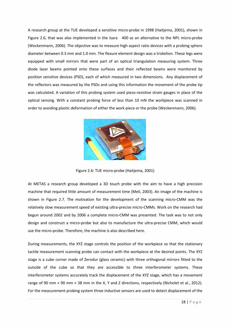
A research group at the TUE developed a sensitive micro-probe in 1998 (Haitjema, 2001), shown in
Figure 2.6, that was also implemented in the Isara 400 as an alternative to the NPL micro-probe
(Weckenmann, 2006). The objective was to measure high aspect ratio devices with a probing sphere
diameter between 0.3 mm and 1.0 mm. The flexure element design was a triskelion. These legs were
equipped with small mirrors that were part of an optical triangulation measuring system. Three
diode laser beams pointed onto these surfaces and their reflected beams were monitored by
position sensitive devices (PSD), each of which measured in two dimensions. Any displacement of
the reflectors was measured by the PSDs and using this information the movement of the probe tip
was calculated. A variation of this probing system used piezo-resistive strain gauges in place of the
optical sensing. With a constant probing force of less than 10 mN the workpiece was scanned in
order to avoiding plastic deformation of either the work piece or the probe (Weckenmann, 2006).
Figure 2.6: TUE micro-probe (Haitjema, 2001)
At METAS a research group developed a 3D touch probe with the aim to have a high precision
machine that required little amount of measurement time (Meli, 2003). An image of the machine is
shown in Figure 2.7. The motivation for the development of the scanning micro-CMM was the
relatively slow measurement speed of existing ultra-precise micro-CMMs. Work on the research had
begun around 2002 and by 2006 a complete micro-CMM was presented. The task was to not only
design and construct a micro-probe but also to manufacture the ultra-precise CMM, which would
use the micro-probe. Therefore, the machine is also described here.
During measurements, the XYZ stage controls the position of the workpiece so that the stationary
tactile measurement scanning probe can contact with the workpiece at the desired points. The XYZ
stage is a cube corner made of Zerodur (glass ceramic) with three orthogonal mirrors fitted to the
outside of the cube so that they are accessible to three interferometer systems. These
interferometer systems accurately track the displacement of the XYZ stage, which has a movement
range of 90 mm × 90 mm × 38 mm in the X, Y and Z directions, respectively (Nicholet et al., 2012).
For the measurement probing system three inductive sensors are used to detect displacement of the
19 | P a g e
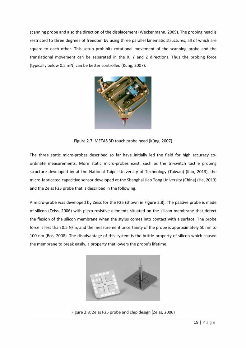
scanning probe and also the direction of the displacement (Weckenmann, 2009). The probing head is
restricted to three degrees of freedom by using three parallel kinematic structures, all of which are
square to each other. This setup prohibits rotational movement of the scanning probe and the
translational movement can be separated in the X, Y and Z directions. Thus the probing force
(typically below 0.5 mN) can be better controlled (Küng, 2007).
Figure 2.7: METAS 3D touch probe head (Küng, 2007)
The three static micro-probes described so far have initially led the field for high accuracy co-
ordinate measurements. More static micro-probes exist, such as the tri-switch tactile probing
structure developed by at the National Taipei University of Technology (Taiwan) (Kao, 2013), the
micro-fabricated capacitive sensor developed at the Shanghai Jiao Tong University (China) (He, 2013)
and the Zeiss F25 probe that is described in the following.
A micro-probe was developed by Zeiss for the F25 (shown in Figure 2.8). The passive probe is made
of silicon (Zeiss, 2006) with piezo-resistive elements situated on the silicon membrane that detect
the flexion of the silicon membrane when the stylus comes into contact with a surface. The probe
force is less than 0.5 N/m, and the measurement uncertainty of the probe is approximately 50 nm to
100 nm (Bos, 2008). The disadvantage of this system is the brittle property of silicon which caused
the membrane to break easily, a property that lowers the probe’s lifetime.
Figure 2.8: Zeiss F25 probe and chip design (Zeiss, 2006)

20 | P a g e
2.2.4.4 Small-scale resonant type micro-probes
Research into resonant type micro-probes began in the early 1990s. The first resonant type micro-
probe implemented in commercial instruments was the Mitutoyo UMAP 130. The CMM stylus could
have a probing sphere diameter of down to 30 μm. The only method of bonding the sphere to the
probe shaft was to melt the sphere onto the shaft (Bos, 2004). This micro-probe detected the
surface regardless of the approach direction – a feature that permitted 3D measurements
(Weckenmann, 2006). The stylus was made to vibrate along the vertical axis by piezo-resistive
actuators. Contact with the surface could be registered by the change of amplitude of the sinusoidal
waveform by the detecting circuit. The resolution was 0.01 μm and the accuracy was less than
0.1 μm (Mitutoyo, 2003).
The NPL are currently developing and optimising a vibrating micro-probe that will be excited at (or
near) its resonant frequency (Claverley and Leach, 2013). Once the prototype exists and its
characterisation is completed, the aim is to implement the micro-probe (shown in Figure 2.9) in the
commercially available Isara 400. This micro-probe’s design is based on the original NPL micro-
probe. It also uses a triskelion design, but instead of capacitors, six patches of lead zirconium
titanate (PZT), which have piezo-electric properties, are in place, two on each leg. Three of the PZTs
(actuators) are used for the vibration control of the stylus and the other three PZTs function as
sensors. When the probe tip approaches a surface, the surface forces damp the vibration amplitude,
which is picked up by the PZT sensors, and a measurement is triggered.
Figure 2.9: NPL vibrating micro-probe (Claverley and Leach, 2013)

21 | P a g e
2.2.4.5 Opto-tactile probing systems
Optical tactile probing systems combine optical technologies with light scattering or reflecting probe
spheres. In Japan and Germany research groups have developed optical tactile probing systems,
which are presented as follows.
The laser trapping probing system developed at Osaka University (Osaka, Japan) used a sphere with
a diameter of 10 μm, which was kept in place by the radiation pressure of a powerful laser, to
provide output data (Michihata et al., 2008; Michihata et al., 2010). The sphere’s surface was
reflective and acted as a mirror in an interferometer system. Thus contact with the workpiece was
registered in response to the change of the interference pattern. The forces that acted on the
workpiece were small (5 mN – 10 mN) and the resolution and accuracy were claimed to be 10 nm
and ± 50 nm, respectively. This technology was designed in particular to measure flat surfaces, which
limited the range of application (Takaya, 2013).
The Physikalisch Technische Bundesanstallt (PTB, Germany) together with Werth GmbH developed
an alternative micro-CMM on the principle of optics (shown in Figure 2.10). The so-called Werth
fibre probe used a glass fibre stylus with one sphere at mid-height of the shaft and the other at its
end. Light was sent through the shaft and was scattered by the spheres. Optical lenses focused on
the scattered light in order to determine the position of the spheres. The sphere at mid-height was
used to trace the position in the Z direction and the sphere at the probe’s tip was used for the
determination of the X and Y positions (Schwenke, 2001). This technique was most suited for the
measurement of holes, however, the techniques suffered from the sticking-effect of the glass fibre
to the workpiece walls. In Figure 2.10 (1) is the sphere for Z positioning, (2) is the mirror, (3) is the
microscope, and (4) is the CCD camera.
Figure 2.10: PTB Werth fibre probe (Schwenke, 2001)

22 | P a g e
Enami from the University of Tokyo (Japan) invented an opto-tactile probe that used a hollow stylus
of 10 mm length through which a helium-neon-laser beam was sent. The beam was reflected off the
mirrored surface of the probe’s sphere that had a diameter of 5 mm (Enami et al, 1999). When a
force was exerted on the probe, the sphere was displaced in the X or Y direction. Thus the laser
beam was reflected in a different angle and reached the sensor, a quadrant photo-detector, at an
offset from the centre of the measuring window. The offset could be related to a force acting on the
probe and hence the point of contact could be detected. A problem was seen for the measurements
in Z direction: when contacting a horizontal surface the sphere did not move sideward and
subsequently no force was measured in the Z direction.
2.2.4.6 X-ray computed tomography technique applied to micro-CMMs
Measurements with the X-ray computed tomography technique return information of the surface as
well as the bulk material of an object. Scanning X-ray tomography, invented by the electrical and
mechanical engineer Sir Godfrey Hounsfield (Beckmann, 2006), reconstructs the object in 3D by
imaging a number of sections at many angles around an axis of rotation (around the object). For
reconstruction, a mathematical procedure called digital geometry processing is applied to the stacks
of images. The imaging technique has been used extensively in radiology (medicine) and biology but
more recently this technique has also been applied to dimensional measurements.
As is the case with tactile micro-CMMs, an X-ray computed tomography micro-CMM cannot simply
be a miniaturised large-scale X-ray computer tomography CMM applied to small objects with
dimensions in the millimetre range. Problems such as insufficient resolution due to the cross section
area of the source must be tackled. Smaller point-like X-ray sources result in more contrasted and
well-defined edges in the image plane.
In 2007 Neuser (Neuser, 2007) from Phoenix X-ray Systems and Services GmbH (Wustorf, Germany)
presented the first high-resolution computed tomography (nanoCT) system, the ‘nanotom’. This
nanotom put a point-like source (‘nanofocus tube’) into practice and an acceleration voltage of
180 kV. The resolution achieved with this system was less than 0.5 μm per voxel. The conditions for
the object are that they are not larger than 120 mm in diameter and not heavier than 1 kg. Since,
higher resolution X-ray systems have been built, such as the Zeiss Xradia 810 Ultra system with a
resolution of 50 nm per voxel (Zeiss, 2013).

23 | P a g e
2.2.4.7 Micro-probes made with the ‘bottom-up’ philosophy: scanning probe microscopy
Scanning probe microscopy (SPM) is a technique that uses a physical probe to scan the surface. This
technique has typically been used for surface topography imaging but it has been credited with the
potential to be implemented in micro-CMMs. Some sub-categories of the SPM technique, such as
non-contact atomic force microscopy (AFM), have the non-destructive nature of measuring in
common with optical techniques. Instruments designed for co-ordinate metrology based on SPM
technology also have the advantage of better resolution over instruments that are based on optical
probes, which are limited by their optical resolution (Weckenmann, 2006). One of the early
approaches to micro-probes based on the technology of SPM was conducted at the University of
Tokyo (Japan).
In 1993, Miasuzawa published his findings on measurements of small holes using a vibrating
scanning method, which he named the ‘vibroscanning’ (VS) technique. This technique used some
features from AFM surface instruments, for example the thin vibrating lever and the exploitation of
the electrical field between the lever and the workpiece. The VS technique used the change in the
vibration amplitude of the lever as an indication of the proximity of the workpiece’s surface. The
vibration amplitude was measured with a voltmeter connected to the object and the vibrating lever
(Masuzawa, 1993). More successfully, Lebrasseur implemented a vibrating scanning technique in an
instrument that was also intended to measure the dimensions of small holes. The vertical vibrating
lever resembled that of an AFM and the change in frequency was controlled and measured by piezo-
actuators and sensors, respectively (Lebrasseur et al., 2000; Lebrasseur et al., 2002).
Research at the PTB has been investigating large range SPM, but it remains that their measuring
range is very small (25 mm × 25 mm × 5 mm in the X, Y and Z axes) (Dai, 2004). This range limits
these instruments’ applicability to very small measurement areas and measurements could only be
completed in 2½D. More recently Dai published the development of a 3D-AFM for true 3D
structures, which presented additional torsional oscillation modes to the traditional vertical
oscillation mode (Dai et al., 2011). This novelty gave the 3D-AFM the ability to measure steep slopes
on micro-structures. Research has continued in this field and the boundary for the measurement
ranges have been pushed to 18 mm in the X and Y direction and 10 mm in the Z direction (Sawano,
2012).
Researchers at the University of Erlangen (Germany) have been concerned with the application of
electrical probing to micro-CMMs (Hoffmann et al., 2008). They designed, realized and tested the
capability of a traditional-looking micro-probe based on electrical probing that is shown in
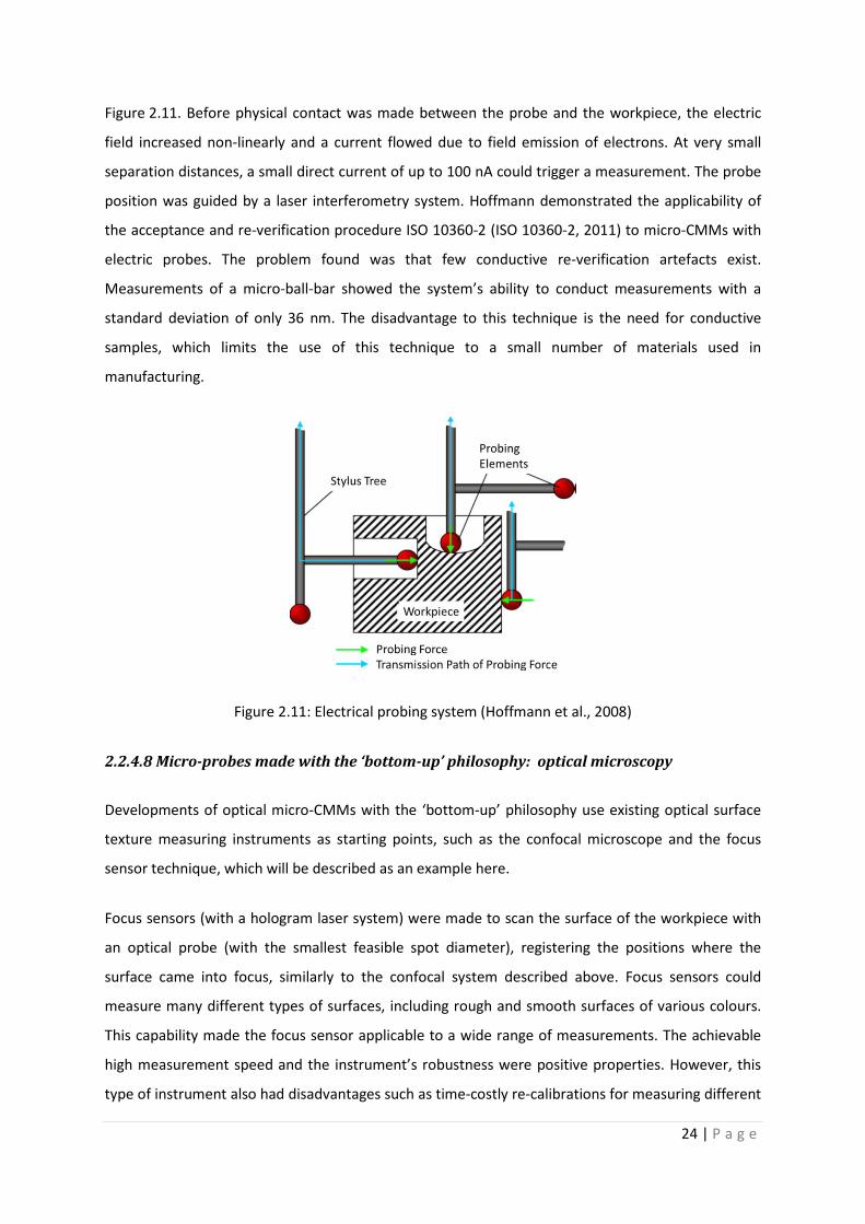
24 | P a g e
Figure 2.11. Before physical contact was made between the probe and the workpiece, the electric
field increased non-linearly and a current flowed due to field emission of electrons. At very small
separation distances, a small direct current of up to 100 nA could trigger a measurement. The probe
position was guided by a laser interferometry system. Hoffmann demonstrated the applicability of
the acceptance and re-verification procedure ISO 10360-2 (ISO 10360-2, 2011) to micro-CMMs with
electric probes. The problem found was that few conductive re-verification artefacts exist.
Measurements of a micro-ball-bar showed the system’s ability to conduct measurements with a
standard deviation of only 36 nm. The disadvantage to this technique is the need for conductive
samples, which limits the use of this technique to a small number of materials used in
manufacturing.
Figure 2.11: Electrical probing system (Hoffmann et al., 2008)
2.2.4.8 Micro-probes made with the ‘bottom-up’ philosophy: optical microscopy
Developments of optical micro-CMMs with the ‘bottom-up’ philosophy use existing optical surface
texture measuring instruments as starting points, such as the confocal microscope and the focus
sensor technique, which will be described as an example here.
Focus sensors (with a hologram laser system) were made to scan the surface of the workpiece with
an optical probe (with the smallest feasible spot diameter), registering the positions where the
surface came into focus, similarly to the confocal system described above. Focus sensors could
measure many different types of surfaces, including rough and smooth surfaces of various colours.
This capability made the focus sensor applicable to a wide range of measurements. The achievable
high measurement speed and the instrument’s robustness were positive properties. However, this
type of instrument also had disadvantages such as time-costly re-calibrations for measuring different

25 | P a g e
materials (Mastylo et al., 2004). A vertical measurement resolution of 1 nm and an uncertainty of
2.7 nm could be achieved (Jaeger, 2010).
2.2.4.9 Micro-probes in summary
The specifications of the three early high-resolution micro-probes are presented in Table 2.3. Of the
three early micro-probes, the METAS micro-probe had the smallest resolution (less than 1 nm) but
the largest moving mass (7 g) and probing force (0.5 mN). The NPL micro-probe had the largest
resolution (3 nm), but the lowest stiffness (10 N/m) and the TUE micro-probe had the smallest
measuring range, the highest stiffness (100 N/m to 450 N/m), the lowest moving mass (20 mg) and
the lowest probing force (less than 1 mN).
Table 2.3: Specifications of three early static micro-probes (Weckenmann, 2006)
Micro-CMM
probe
Resolution
(nm)
Measuring range
(μm)
Stiffness
(N/m)
Moving mass
(mg)
Probing force
(mN)
NPL micro-
probe 3 ± 20 10 370 0.2
TUE micro-
probe 1 25 100 - 450 20 < 1
METAS < 1 ± 100 20 7000 0.5
The following table (Table 2.4) presents a collection of specifications for the remaining micro-probes
that were not included in Table 2.3, but mentioned in the previous text. Some of these micro-probes
are still in the development stage and specifications have yet to be published in the literature. The
number of missing data demonstrates the difficulty of comparing the micro-probes.

26 | P a g e
Table 2.4: Specifications (where available) of more recent micro-probes
Micro-CMM probe Resolution
(nm)
Accuracy
(nm)
Uncertainty
(nm)
Measuring
range
(μm)
Probing
force
(mN)
Repeata
bility
(μm)
‘Vibroscanner’
(Masuzawa, 1993) - - - - 1 -
Mitutoyo UMAP
(Mitutoyo, 2003) 10 < 100 200 200 150 -
Zeiss F25 micro-probe
(Bos, 2008) - - 50 – 100 - < 500 -
NPL vibrating micro-
probe - - - - - -
Laser trapping probe
(Michihata et al., 2008) < 10 < 50 - - 5 - 10 64
Werth FibreProbe
(Weckenmann, 2006) 0.1 50 300 ± 400 0.5 <10
Enami opto-tactile probe
(Enami, 1999) - - - - - <10
Nanotom
(Neuser, 2007) 500 3000 - - - -
PTB LR-SPM
(Dai, 2004) 0.1 - 0.7 - - 0.001
Focus sensor
(Jaeger, 2010) 1 - 3 ± 3 n/a -
Tri-switch tactile
(Kao, 2013) - - 80 - - 0.19
Micro-fabricated
capacitive sensor
(He, 2013)
10 (Axial)
25 (radial) - - - - -

27 | P a g e
2.3 Surface metrology
Although the aim of this research was to explore the applicability of a new technique to a micro-
CMM, a short review of surface metrology is presented here because the new technique (focus
variation) that was investigated was originally applied to surface metrology. This section should give
an understanding to why the FV technology was chosen for this research.
2.3.1 The story of surface metrology
Surface metrology is the science of surface measurements and any surface topography measuring
instrument is a tool in the research and measurement of surfaces. Automated surface topography
devices give physical representations of surfaces. In comparison to co-ordinate metrology, the story
of surface metrology does not reach back so far in time and only started to become more significant
before the turn of the 20th century, when surface finish of manufactured parts started to become
increasingly more important with the development of precision manufacturing. This fuelled the
advancement of the tools used in surface metrology.
Up until the 20th century, surface finish was judged by sight and touch. This method of describing the
surface is qualitative and generally not quantitative. However, when it became clear that the surface
characteristic played an important role in part functionality, a manufacturing company, attempting
to control production, assembled a scale of differently finished samples in a case. The idea was that
the workmen could use these samples as references for their manufactured surfaces (Shaw, 1936).
This comparative method of controlling the surface finish was still based on appearance and did not
give a quantitative measure to the surface roughness. Figure 2.12 shows one of the early roughness
scales.
Figure 2.12: Roughness scale (Shaw, 1936)
In a similar manner to the history of co-ordinate metrology, the pressure for increased accuracy in
surface topography assessment came from the automotive industry, where it was becoming
apparent that the surface had a very important role in the durability of engines, accuracy of parts
being built into the components generating power and the noise level of the cars (Harrison, 1931).

28 | P a g e
Some efforts were completed to measure surface roughness, but the methods invented could not be
sustained due to their complexity. Here is an example of one such method: the inverse of the
surface was obtained using gelatine or celluloid, which after disconnecting it from the workpiece,
was cut up in fine strips. A surface profile was then obtained by photographing the edge of a strip
horizontally and magnifying the image (Schmaltz, 1929). Other simpler methods included the use of
microscopes, which were introduced long before by Leewenhoek in 1660 (Schwenke et al, 2002) but
had not yet been applied to surface metrology.
In the 1920s, the first significant surface measuring instrument, a surface profiler, was invented by
the German engineer Schmaltz, who later contributed to the development of roughness surface
parameters and flatness characterisation (Schmaltz, 1929). His surface profile measuring instrument
consisted of a sapphire needle, attached to a pick-up arm, which was dragged over the surface
(Shaw, 1931). The vertical movement of the arm was recorded by attaching a lightweight mirror to
the pivoted stylus: a light beam was redirected by the mirror to a moving photographic chart. The
position and angle of the mirror directed where the light beam would hit the photographic chart and
thus a (distorted) profile was drawn (Leach, 2010).
The benefit of such instruments at the time was the quantitative assessment of the surface,
however, it was a slower process than the comparative method, the instrument was more expensive
to acquire than roughness scales, and the calibration procedure difficult (Harrison, 1931). In addition
the accuracy of the instruments depended on too many variables such as the speed of motion of the
sapphire point (Shaw, 1936).
A British company Taylor, Taylor and Hobson (TTH) have had a significant influence on contact
surface measuring instruments and are to date one of the leading companies in this industry. They
were involved in metrology before the First World War by producing screw diameter measuring
machines, which proved to be successful especially in the armaments manufacturing industry
(Leach, 2010; Taylor and Hobson, 2013). In the mid-1930s they started making stylus instruments,
which they named profilographs. The profilographs have (since their invention) not changed
dramatically in their hardware design. The novelty was mainly the sensors, the sensitivity of the
sensors and eventually the software.
Optical surface measuring instruments were also invented at approximately the same time as tactile
surface measuring instruments. Optical techniques such as the Michelson and Twyman-Green
interferometers were applied to inspection of surface form and roughness: Schmaltz was the first to
use a light sectioning microscope for surface analysis (Schmaltz, 1929), Linnik, who was employed at

29 | P a g e
the Mendellief Institute in Leningrad (1930), introduced the micro-interferometer (Miroshnikow,
2010), Tolansky used the multiple beam interferometer (Tolansky, 1960), and a method using fringes
of equal chromatic order (FECO) interferometers was made known by Bennett (Bennett, 1976).
The advancement of computing in the second half of the 20th century revolutionised surface
measuring instruments: automated measurements were now possible. The first instrument that was
able to perform automatic measurements was the phase shifting interferometric (PSI) microscope,
which was made in the early 1980s (Bhunshan et al., 1985). The microscope was controlled by a
micro-computer and areal measurements were processed by a desk-top computer. In the early
1990s a confocal microscope was automated (Schmidt et al., 1992), and this innovation was followed
by the automation of coherence scanning interferometric (CSI) microscope (Caber, 1993). With the
possibility of automating the instruments, the measurement and post-process time could be
shortened dramatically.
By digitising the measurement results (i.e. profiles, surfaces) the analysis of profiles and surfaces
could become more sophisticated. Whilst previously a surface’s mean height of the roughness was
estimated, with the help of computers the mean surface height could be calculated automatically
and with a better accuracy. Additionally height variations of surfaces could be categorised in terms
of roughness, waviness and form, which were distinguished by the spatial frequency of the height
variation. Roughness was defined as having the highest spatial frequency and form as having the
lowest spatial frequency. The computer provided the opportunity to mathematically process the
profile or surface with different algorithms thus obtaining different values with which specific
characteristics of the surface could be described. Many parameters now exist, some of which are
identified in Tables 2.5 and 2.6.
Table 2.5: Examples of surface roughness (R) profile parameters (ISO 4287, 2000)
Parameter Description Typical Units
Ra Arithmetical mean height µm
Rq Root mean square length of the roughness profile µm
Rsk Skewness of the roughness profile -
Rku Kurtosis of the roughness profile -
Rp Maximum peak height µm
Rv Maximum pit depth µm
Rz Maximum height of the roughness profile µm
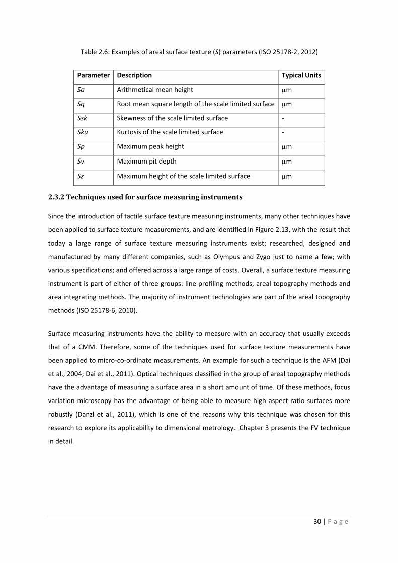
30 | P a g e
Table 2.6: Examples of areal surface texture (S) parameters (ISO 25178-2, 2012)
Parameter Description Typical Units
Sa Arithmetical mean height µm
Sq Root mean square length of the scale limited surface µm
Ssk Skewness of the scale limited surface -
Sku Kurtosis of the scale limited surface -
Sp Maximum peak height µm
Sv Maximum pit depth µm
Sz Maximum height of the scale limited surface µm
2.3.2 Techniques used for surface measuring instruments
Since the introduction of tactile surface texture measuring instruments, many other techniques have
been applied to surface texture measurements, and are identified in Figure 2.13, with the result that
today a large range of surface texture measuring instruments exist; researched, designed and
manufactured by many different companies, such as Olympus and Zygo just to name a few; with
various specifications; and offered across a large range of costs. Overall, a surface texture measuring
instrument is part of either of three groups: line profiling methods, areal topography methods and
area integrating methods. The majority of instrument technologies are part of the areal topography
methods (ISO 25178-6, 2010).
Surface measuring instruments have the ability to measure with an accuracy that usually exceeds
that of a CMM. Therefore, some of the techniques used for surface texture measurements have
been applied to micro-co-ordinate measurements. An example for such a technique is the AFM (Dai
et al., 2004; Dai et al., 2011). Optical techniques classified in the group of areal topography methods
have the advantage of measuring a surface area in a short amount of time. Of these methods, focus
variation microscopy has the advantage of being able to measure high aspect ratio surfaces more
robustly (Danzl et al., 2011), which is one of the reasons why this technique was chosen for this
research to explore its applicability to dimensional metrology. Chapter 3 presents the FV technique
in detail.

31 | P a g e
Figure 2.13: Technologies of surface texture measuring instruments
(adapted from ISO 25178-6, 2010)
2.3.3 Calibration artefacts for optical surface texture measuring instruments
With the prospect of applying an areal optical technique, originally used for surface texture
measurements, to dimensional measurements, it is important to understand how the performance
of such surface texture measuring instruments is assessed. A number of calibrated artefacts exist to
assess the performance of areal optical surface texture measuring instruments. Most commonly
these calibrated artefacts are two dimensional but three dimensional artefacts exist as well. An
example for a calibration artefact for areal surface texture measure is the checker-board pattern,
with which the resolution and the measurement accuracy can be verified. Calibration artefacts that
are three dimensional have variations in the third dimension (Z) that are either very small (in the
nanometre range) or large (in the millimetre range).
The NPL developed a series of artefacts for the calibration of areal surface texture measuring
instruments, referred to as the ‘bento box’. The areal cross grating depicted on the left of
Figure 2.14 is used for the calibration of the XY axes’ amplification and squareness by measuring the
positions of the centre of gravity of each square formed by the cross grating (Leach and Giusca,
2012). The areal star pattern (right of Figure 2.14) with a height variation of 50 nm is used to

32 | P a g e
determine the lateral period limit (“the spatial period of a sinusoidal profile at which the height
response of an instrument falls to 50 %” (ISO CD 25178-600, 2013)) of an optical instrument (Giusca
and Leach, 2013(a)).
Figure 2.14: NPL areal calibration artefacts: areal cross grating and areal star pattern (NPL, 2013)
There are two options for the performance assessment of a future FV micro-CMM: either a re-
verification route similar to calibration methods of areal surface texture measuring instruments is
taken, or the FV micro-CMM is assessed by methods that have been used for CMMs. This decision
requires an investigation of existing standards for the re-verification of CMMs and of existing re-
verification artefacts used for micro-CMMs.
2.4 Re-verification of CMMs
2.4.1 Introduction
Metrology is a wide field of research, which incorporates legal metrology, next to other classes of
metrology such as applied metrology, quality metrology and theoretical metrology. Legal metrology
treats the units of measurements, the methods of measurements and the measuring instruments in
relation to legal requirements (BS 5233, 1986). Institutes that address legal metrology have the
objective to ensure a public guarantee for an appropriate accuracy of measurements. Until the
standard unit of length was defined, it would have been a very difficult task to ensure the accuracy
of measurements. The BIPM was the first institute to pave the way to a standardisation of length
measurements, firstly by defining the metre, the story of which has been identified earlier, and then
by writing international standards for metrology. These standards comprise definitions of
traceability, calibration, acceptance test, re-verification test, and health check, which are of
importance here and are as follows (BS 5233, 1986; ISO 10360-1, 2000).

33 | P a g e
Traceability: “the property of a result of a measurement whereby it can be related to appropriate
standards, generally international or national standards, through an unbroken chain of comparisons”
Calibration: “the set of operations which establish, under specified conditions, the relation between
values indicated by a measuring instrument or measuring system, or values represented by a
material measure, and the corresponding known values of a measurand”.
Acceptance test (of a CMM): “set of operations agreed upon by the CMM manufacturer and the user
to verify that the performance of a CMM is as stated by the manufacturer.”
Re-verification test (of a CMM): “test to verify that the performance of a CMM is as stated by the
user and executed according to the same procedures as those of the acceptance test.”
Interim check (of a CMM) / health check: “test specified by the user and executed between re-
verifications to maintain the level of confidence in the measurements taken on the CMM.”
Traceability ensures that all manufacturing and measurements of parts is completed with respect to
the same standard length, e.g. the metre at the NPL. This is of great importance when parts with
tight manufacturing tolerances have to fit into an assembly of other parts, e.g. a motor.
For linear measuring instruments, such as a scale for example, a calibration procedure is straight
forward, because it only has one degree of freedom (DoF). However, for 3D measuring instruments,
such as CMMs, calibration becomes a very long-winded process, because of multiple DoFs and no
single practical calibration method has yet been designed that fulfils all requirements of a
calibration.
A user’s interests lies partly in the knowledge of the true machine performance but more
importantly in the confidence of the machine. For that reason, performance evaluation methods
(acceptance and re-verification procedures) exist, some of which will be presented more extensively
in the following sections.
Today international standards exist for the acceptance and re-verification of many types of
metrology instruments and standards are still in the process of being written for instruments that
bear technologies that have been introduced to metrology in recent years. The international
standard concerned with the acceptance and re-verification of CMMs is the ISO 10360 series, which
addresses CMMs used for measuring size (ISO 10360-2, 2009), CMMs with a rotary table as the
fourth axis (ISO 10360-3, 2000), CMMs used in scanning measuring mode (ISO 10360-4, 2000),

34 | P a g e
CMMs using multiple-stylus probing systems (ISO 10360-5, 2010), CMMs equipped with imaging
probing systems (ISO 10360-7, 2011), CMMs with optical distance sensors (ISO 10360-8, 2013),
CMMs with multiple probing systems (ISO 10360-9, 2013), CMMs equipped with laser trackers (ISO
DIS 10360-10, 2013), and CMMs with an articulated arm (ISO CD 10360-12, 2013).
The result of an acceptance and re-verification procedure gives an indication of an instrument’s
measuring capability. These results should be compared to the machine tolerances provided by the
instruments manufacturer. Any values that lie outside the tolerance indicate that the instrument
cannot measure within the uncertainty band specified by the manufacturer. For any type of
performance evaluation test of a machine, the environmental conditions in which the machine is
situated must be considered when evaluating the results.
2.4.2 Calibration, acceptance, re-verification and health-check tests for CMMs
Four procedures that all give information on the instrument position accuracy are distinguished here
in more detail: calibration, acceptance test, re-verification and health-check. There are very
important differences between these four terms, which are discussed in the following. In the context
of this research, regularly performed tests, namely the re-verification and the health-check, are of
interest.
Calibration is the process required to allow measurement uncertainty to be assessed. For a CMM, a
calibration is not as straightforward as described in the example above. A traditional tactile CMM for
instance has 21 sources of geometric error (18 path-dependent errors and 3 squareness errors) and
those errors are different depending on the variables of a measuring task (Busch et al., 1985). The
now withdrawn PTB standard, VDI/VDE 2600 (VDI/VDE 2600, 1973), presented one of the first
suggested procedures for a full calibration of a CMM. The essence of this calibration procedure was
as follows.
A mathematical model of the CMM (a virtual CMM) should be created, describing the interaction of
all error components that influence a measurement. All error components used in the model should
then be measured on the CMM and fed into the model. With the mathematical model, multi-
dimensional errors and their effects on single measurements can be computed. The machine’s
uncertainty for single measurements and for variables of measuring tasks should also be fed into the
model. Finally, the results of the model should be compared to the results of a rigorous set of
measurements on the CMM.

35 | P a g e
With the advance of technologies, the scales of a CMM can be calibrated with increasingly smaller
uncertainties and with increasing larger number of data points per volume; however, it remains that
a calibration procedure is very time intensive because of the CMM’s three dimensional nature of
measurements. The development of laser trackers, for example, has made them applicable to CMM
calibration: a retro-reflector replaces the probe and it is positioned at certain measurement points in
the measuring volume in order to create a map of measurement points.
Given that genuine calibration of CMMs is very time consuming, complicated and expensive, users
tend to the acceptance and re-verification tests because they are easier, simpler, faster, and
cheaper. An acceptance test and re-verification test establishes whether a CMM performs within the
performance specification for a certain task. The difference between these two tests is the point in
time when they are performed: an acceptance test is performed by the instrument manufacturer
before the instrument is sold to the customer to prove that the machine’s measurement capability is
within the specification (maximum permissible error (MPE) given by the manufacturer), and the re-
verification test is usually a repeat of the acceptance test once a year, in order to establish if the
machine still meets the uncertainty specification. In principal any task can be chosen for the purpose
of an acceptance and re-verification test, if the manufacturer and the customer agree, but standards
such as the ISO 10360 series, document suggestions for acceptance and re-verification tests. These
standards hold a very important place for many instrument manufacturers. Acceptance and re-
verification tests are typically completed by an expert within a day and it is normally repeated
yearly. In the case when the machine is found faulty it is generally the manufacturer’s responsibility
to re-establish a good performance of the machine.
A health check (or interim check) should be performed more frequently on CMMs than a re-
verification procedure. To some extent a health check is similar to a re-verification: both give an
indication of machine accuracy for a task-specific performance. The difference between these two
tests lies with the measurement task; the health check is a simple and short measurement routine,
which can be easily executed by a user, and which usually take half an hour to be completed. Some
instrument manufacturers, such as Renishaw, can provide equipment and suggest a method for a
health check (Renishaw, 2007), but the user can choose a task more closely related to the commonly
performed measurements on the CMM.
Every part of the ISO 10360 document, suggests artefacts suitable for the execution of an
acceptance, re-verification and health check, amongst which the most commonly used are gauge
blocks, ball bars and length bars.

36 | P a g e
2.4.3 Environmental considerations
The environment influences the performance of any measuring machine. Depending on the accuracy
and precision these influences may be problematic. In the case of precise measuring instruments,
e.g. CMMs, the following factors, which have been specified in the British standard BS 6808-3 (BS
6808-3, 1989), should be taken into consideration. This standard was written specifically for CMM
users, but the environmental considerations may be equally applicable to surface topography
instruments.
Vibration analysis: Vertical and horizontal vibrations must be tested before a CMM is handed to the
user in order to certify whether the responsibility for faults is the user’s or the manufacturer’s. All
possible sources of vibration from the machine itself must be tested. These include the motor, if
existent, or the air-bearing stability. Should these be sources of vibrations exceeding the
specifications, then the supplier must modify the instrument. If the vibrations do not originate from
the instrument itself, but from the support system of the CMM instead, then the support system
must be inspected which can be done by attaching three transducers in all three axes. In this case, it
is the user’s duty to correct the problem.
Air supply: The air supply can cause errors in measurements. In order to measure characteristics of
the air supply measuring instruments such as an air pressure gauge with an accuracy of ± 5 %, an air
flow gauge with an accuracy of ± 20 % of the maximum flow rate specified by the supplier and a
temperature calibrated measuring system to an accuracy of ± 0.1 °C are needed. With these
instruments the pressure fluctuations, support pressure and flow, the air supply temperature and
contamination can be measured.
External temperature influences: Ideally, the temperature of the CMM and the workpiece remains
temporally and spatially constant and is fixed to 20 °C. (BS EN ISO 1, 2002). Sources of influences are
sunlight, neighbouring instruments, radiation or the proximity of the operator if applicable.
Corrections to the effects of temperature should be done by calculations based on known thermal
parameters of the CMM and the workpiece and with the assumption that the temperature is
constant in space and time. Workpieces should not get into contact with objects that have a
different temperature, as a change in dimension is the consequence that will not correct itself soon
after.
Other machine influences: The material of the work piece plays a role in the measurement’s errors. If
the workpiece is too soft and an inappropriately strong probing force is applied, then the probing

37 | P a g e
sphere may become impressed in the workpiece. The maximum permissible deadweight of a
workpiece must be specified for instruments that rely on dynamic measuring systems.
2.4.4 Review of re-verification artefacts for micro-CMMs
The performance of a CMM should be verified and periodically re-verified. For this purpose,
reference artefacts are chosen. Ideally, the same artefact should be used for the verification and the
re-verification and it should have the required mechanical perfection of the length-defining features,
a certified accuracy, dimensional stability and mechanical rigidity (BS 6808-3, 1989). According to ISO
10360, the calibration artefact’s accuracy must be more than 20 % of the measuring instrument’s
accuracy. Artefacts for task-specific health checks are usually objects that are of the shape and
material of the common workpiece. Frames are a popular choice of artefacts. Examples of these
artefacts are rigid space frames or synthetic space frames, such as ball ended bars. In the following a
number of reference artefacts used for micro-CMMs will be presented.
2.4.4.1 Ball Plates and 2D artefacts
The Zeiss miniature hemisphere plate
A hemisphere plate artefact shown in Figure 2.15(a) has been designed specifically to verify micro-
CMMs with tactile micro-probes, and to be calibrated by the Zeiss F25 at the PTB. The artefact’s base
plate was made of Zerodur (90 mm x 90 mm x 5 mm) and the 5.6 mm radius hemispheres were
made of silicon nitride (Si3N4). Zerodur has a very low thermal expansion and is, therefore, a
particularly suitable material for a verification artefact. Nine hemispheres were wrung onto the
Zerodur plate and placed into specific positions so that 36 lengths could be measured ranging from
13 mm to 100 mm (Neugebauer, 2010).
CMMs that were to be re-verified with the hemisphere plate were expected to have a maximum
permissible error (MPE) not less than 300 nm. The artefact was calibrated at the PTB with the Zeiss
F25 micro-CMM, which has an MPEE statement of (0.25 + L/666) μm. The calculated expanded
measurement uncertainty (using a coverage factor of k = 2) was equal to 80 nm for both the X and
the Y axes (Ux, Uy) and the uncertainty of the distance measurement in between hemisphere centres
(UL) was 110 nm (Neugebauer, 2011).
Despite the smaller errors of the Zeiss F25 than those micro-CMMs, for which the re-verification
artefact was designed for (e.g. the O-INSPECT by Zeiss), systematic errors of the Zeiss F25 were
found to be unacceptable for the calibration of the hemisphere plate. In order to eliminate the

38 | P a g e
influence of these errors, holes were positioned in the Zerodur-plate, so that every hemisphere
could be measured from below close to its equator, as depicted in Figure 2.15(b). By measuring the
hemispheres’ positions from the top, from below, at 90 degrees and at other angles, the systematic
deviation of the Zeiss F25 CMM could be minimised by applying an error separation technique
developed at the PTB.
The calibration uncertainty after the separation of systematic error reduced to 50 nm with a
coverage factor of k = 2 and the long-term reproducibility of the calibration method showed small
deviations of ± 15 nm (Neugebauer, 2011).
(a) (b)
Figure 2.15: (a) Zeiss hemisphere plate; (b) two approach directions by tactile micro-probe
(PTB, 2012)
PTB micro-ball plates
The micro-ball plate artefacts have been made by the PTB and were designed to test optical as well
as tactile micro-CMMs. In order to be applicable to various optical techniques such as
interferometric sensors or focus variation sensors, one artefact featured a smooth surface (Figure
2.16(a)) and the other artefact had a rough (diffuse reflecting) surface (Figure 2.16(b)). Although the
spheres incorporated in the artefact had to be measured in 3D, the measurands (lines connecting
sphere centres) all lay within the XY plane of the measuring instrument and thus the artefact was
classified as a 2½D verification artefact.
The smooth artefact had an array of 6 x 6 steel spheres each with diameter of 2 mm and a
separation between neighbouring spheres of 4 mm. The spheres were clamped into place from the
bottom side by using springs as shown in Figure 2.17(a).
The rough artefact had an array or 6 x 6 roughened steel spheres, with diameters of 0.5 mm, and
separation distances of 1.3 mm. Each of the spheres was adhesively bonded in conical impressions

39 | P a g e
as shown in Figure 2.17(b) (Ehrig and Neuschaefer-Rube, 2007). The roughening of the spheres
required a lapping technique: the steel spheres were put into an ultrasonic bath with a polishing
agent that roughened the spheres to a roughness (Rz) of approximately 1 µm (Neuschaefer-Rube et
al., 2008).
The ball plate artefacts could be used for probing errors of size and form as well as length
measurement errors. ISO 10360 for the acceptance and re-verification of CMMs suggests the use of
a sphere for the assessment of probing error, which can be completed with the ball plates. However,
the re-verification of error of indication for size measurement could not be performed with the ball
plate because the measurands lay in the XY plane and therefore, the volumetric diagonals could not
be assessed.
(a) (b)
Figure 2.16: (a) PTB smooth ball plate; (b) PTB rough ball plate (Neuschaefer-Rube et al., 2008)
(a) (b)
Figure 2.17: (a) Fixing principle with pressure springs; (b) adhesively bonded spheres
(Ehrig and Neuschaefer-Rube, 2007)
Column (cylinder) plate, ball plate and insert hole plate
The National Measuring Institute of South Africa (NMISA) has developed a number of verification
artefacts that can be applied to touch-probe and optical micro-CMMs. The artefacts fulfil the
predefined criteria set by the NMISA: they have a long-term stability; they are measureable by both

40 | P a g e
tactile and vision systems; they have geometric features; they have a known thermal expansion
coefficient; and they cover an area of approximately 100 mm × 100 mm.
In the process of selecting the basic concepts of the artefacts a number of designs were considered.
The hole plate design was rejected because of poor edge machining, which impairs the
measurements completed by vision systems. Three other artefact types were tested and found
suitable as verification artefacts for micro-CMMs: the cylinder (column) plate, the ball plate, and the
insert hole plate (Kruger et al., 2011).
The development of the cylinder (column) plate (Figure 2.18(a)) originated from the idea of the hole
plate. It was found that the edges of cylinders can be machined to a much higher accuracy than the
edges of holes. The hole plate was converted to a cylinder plate by placing cylinders (all of the same
height) into the holes, thus creating an array of 5 x 5 columns. The downside to this design is that
the cylinder plate cannot be measured from both sides (top and bottom). This does not affect the re-
verification procedure of the micro-CMM but it affects the calibration of the artefact itself because
the systematic deviation of the CMM cannot be eliminated, or at least diminished enough, by using
the reversal technique (Trapet et al., 1991), whereby the artefact is measured in different
orientations in order to eliminate systematic errors of the CMM.
The sphere plate (Figure 2.18(b)) was based on the design of the Koba sphere plate made by Kolb &
Baumann GmbH (Kolb and Baumann, 2013) for CMMs. The micro-sphere plate design showed clear
advantages for touch probe systems, however, for vision systems there was a lack of clear edges.
Other optical systems, such as the CSI, could be verified with this type of artefact.
The last artefact designed at NMISA was the inserted hole plate (Figure 2.18(c)). So rather than
having drilled holes similar to the first of the NMISA artefacts presented above, holes made of
ceramic were inserted into the base. The inserts could be manufactured to a higher accuracy of
roundness (1 μm) by grinding methods.

41 | P a g e
(a) (b) (c)
Figure 2.18: (a) Cylinder (column) plate; (b) sphere plate; (c) hole plate with ceramic inserts
(Kruger et al., 2011)
In Table 2.7 is a comparison between the so-called KOBA sphere plate and the NMISA micro-sphere
plate. Information from the Zeiss hemisphere plate and the two PTB ball plates has been added to
the table for comparison purposes.
Table 2.7: Characteristics of sphere-plates
Features KOBA ball plate NMISA
micro-
sphere plate
Zeiss
hemisphere
plate
PTB smooth
ball plate
PTB rough
ball plate
Application Re-verification of
CMMs
Re-
verification
of micro-
CMMs
Re-verification
of micro-
CMMs
Re-
verification of
micro-CMMs
Re-
verification of
micro-CMMs
Size of
artefact
230 mm x 230 mm
x 24 mm, 620 mm x
620 mm x 24 mm
100 mm ×
100 mm ×
5 mm
90 mm ×
90 mm ×
5 mm
40 mm ×
40 mm ×
10 mm
30 mm ×
30 mm ×
10 mm
Substrate
material
Steel, stabilised by
long ageing process
Steel Zerodur glass
ceramics
Steel Steel
Symmetry Symmetric
(5 x 5)
Symmetric
(5 x 5)
Not symmetric Symmetric
(6 x 6)
Symmetric
(6 x 6)
Fixture of
spheres
Distortion free,
prism shaped,
retention, access to
equator
access to
equator
Wringing Pressure
springs
Adhesively
bonded

42 | P a g e
Sphere
diameter,
material
-,
ceramic
-,
steel
5.6 mm, - 2 mm,
steel
0.5 mm,
steel
Accuracy <0.3 μm - 50 nm - -
Accessibility
of spheres
From both sides From both
sides
From both
sides
From top
only
From top
only
Sandia silicon standard
At the US Sandia National Laboratory reference artefacts have been designed with the particular
intention of making them suitable for re-verification of micro-CMMs with multiple sensor systems:
touch-probe and vision system based. The micro-machined artefacts (Figure 2.19(a-c)) are,
therefore, referred to as hybrid artefacts (Tran et al., 2007). They were made of monolithic silicon
crystals and feature shallow three dimensional structures for the touch probe measurements and
very sharp edges for optical measurements. The sharp edges could be realised by taking advantage
of the crystalline nature of the silicon: the artefacts were made of a micro-machined single-silicon-
crystal bulk that was etched in an alkaline solution (e.g. potassium hydroxide). This method led to
particularly sharp edges because the etchant did not have sufficient energy to break through strong
crystallographic planes and created sidewalls with exact angles of 54.74 degrees. This technique
gave the novel artefacts nanometric sharpness along the edges. The uncertainty of the artefact was
estimated at 100 nm.
These silicon artefacts had another considerable advantage over other reference artefacts, such as
chrome-on-glass artefacts, designed for vision sensors: the production costs were lower and as a
result they could be sold for a lower price. However, one drawback to this technique was that
curved features were not feasible. This limited the variability of the designs of the 3D artefacts and
thus makes this technique unsuitable for a re-verification artefact that conforms to ISO360, which
specifically notes that a sphere or a circular artefact must be measured to identify the probing error.

43 | P a g e
(a) (b) (c)
Figure 2.19: (a-c) Three designs of Sandia silicon standards (Tran, 2008)
PTB calotte plate
The PTB designed the calotte (concavity in the form of a niche or cup) plate (Figure 2.20) as a 2½D
artefact with the main objective of making comparisons between CT scanning instruments and
multi-sensor measuring instruments (tactile and optical) (Neuschaefer-Rube, 2008). To conform to
the CT technique, the calotte plate was made of Zerodur and manufactured by grinding and
polishing methods. The calotte plate featured an array for 4 × 4 calottes, which had diameters of 3
mm each. The distances between the calottes were measured at the PTB with a tactile CMM and the
results showed a deviation of 1.5 µm from the nominal (1.6 mm) and a form error of 2.5 µm. The
measurement results with CT instruments did not show results as good as these; however, taking
the voxel size into account, sub-voxel accuracy was achieved with the CT instrument.
Figure 2.20: 2½D calotte plate (Neuschaefer-Rube, 2008)
2.4.4.2 Task specific artefacts
In many cases it is beneficial to re-verify a measuring instrument using an artefact that is similar to
the objects that are measured on daily basis. The PTB has recently developed three task-specific
artefacts: the micro-contour standard, the micro-gear standard, and the micro-hole standard, all of
which are presented here. The disadvantage of task specific artefacts is that they are only useful for

44 | P a g e
a limited number of applications and the aim of this research is to eventually produce a re-
verification route that is more general and has broader applicability.
2D micro-contour standard
This specific micro-contour standard, depicted in Figure 2.21, was introduced by the PTB with the
aim to conform to VDI/VDE 2629-1 (VDI/VDE 2629-1, 2008). The design was taken from a contour
standard but adapted to re-verify micro-sensors, such as the FV instrument. The reference standard
features 13 geometric shapes that are paired, to name a few: a full half-cylinder and a hollow half-
cylinder, a ridge and a grove with sidewalls at 45 degree angles, and a ridge and a grove with
sidewalls at 60 degree angles. Additionally to the heights and depths, other features for example
roundness, roughness and distances could be measured on the micro-contour standard and thus the
number of measurable features amounted to 150. Table 2.8 lists the shapes present on the micro-
contour standard and indicates their dimensions.
The standard was manufactured using wire-EDM techniques, which left behind a rough surface with
a Rz value of approximately 1 µm (Ehrig, 2009). This surface characteristic was ideal for optical
instruments, especially those that need a certain roughness on the object to function well (e.g. FV
instruments). For optical measuring instruments the micro-roughness was beneficial because a
surface at a high angle such as 70 degrees could be measured due to the diffuse reflection.
Figure 2.21: PTB 2D micro-contour standard (Ehrig, 2009)

45 | P a g e
Table 2.8: PTB micro-contour standard: features and dimensions (Ehrig, 2009)
Shape Height / Depth
(mm)
Cylinder 1
Ridge/groove (45 degree) 1
Ridge/groove (60 degree) 1
Ridge/groove (80 degree) 1
Cylinder 0.5
Ridge/groove (45 degree) 0.5
Ridge/groove (60 degree) 0.5
Ridge/groove (80 degree) 0.5
Flat (Ra) 0.1
Step-height 0.25
Step-height 0.5
Step-height 0.75
Step-height 1
Micro-gear standard
The micro-gear standard shown in Figure 2.22 was also a result of PTB’s research into task specific
standards for tactile and optical micro-sensors. This standard was a collection of micro-planetary
gears, which had an outer diameter of six millimetres (Neuschaefer-Rube, 2008). Three rough
spheres with 2 mm diameters were mounted on the plate as well, in order to allow overlapping of
measurements taken in different orientations. The cut-outs of the substrate permitted
measurements with techniques that used backlight illumination. The halved ring gear and the
satellite gear with two removed gear teeth were added to the assembly of micro-gears to ensure
that there was a direct view onto every surface (Neuschaefer-Rube, 2008).
Figure 2.22: PTB micro-gear standard (Neuschaefer-Rube, 2008)

46 | P a g e
Micro-hole standard
The micro-hole standard seen in Figure 2.23 has also been invented by the PTB as a task specific
standard. It has been designed to verify the performance of instruments – most commonly the fibre
probe (Neuschaefer-Rube, 2008) - that inspect holes such as injection nozzles. The artefact is built up
by a number of sheets, each with four through holes: three for the bolts and one which is the micro
hole. By stacking them in order, a micro-hole as deep as two millimetres and with a width of 125 µm
is created. In order to define the rotational orientation and the order, each of the sheets have two V-
grooves on the edge and when the sheets are assembled correctly, there is one continuous vertical
V-groove and one tilted V-groove along the side of the artefact.
Figure 2.23: PTB micro-hole standard (Neuschaefer-Rube 2008)
2.4.4.3 Other artefacts
3D calotte cube
The calotte cube (Figure 2.24) was designed at the PTB and had features that are very similar to the
calotte plate. It had an edge length of 10 mm and was made of a titanium alloy (Ti6Al4V). The hole-
pattern which is ideally identical on three surfaces (that share one corner) is a two dimensional array
(5 × 5) of spherical calottes (radius 400 µm). The concave calottes are 1.6 mm apart in the X- and the
Y-direction. The calotte cube was manufactured by the German company IMM Mainz GmbH by using
a sink and wire erosion technique (Neuschaefer-Rube et al., 2008) and is commercially available. The
surface finish has a micro-roughness, a property that makes the artefact suitable to a wider range of
instruments. Calibration was completed at the PTB with an approximate uncertainty of 1 µm for the
distances in between the calottes.
The artefact was designed to be measurable with a variety of technologies: optical, tactile, CT-
scanner and multi sensors (tactile and optical). However, for optical instruments the calotte cube is
merely a 2D or 2½D artefact because the optical instruments cannot measure the vertical sides of
the cube. The artefact’s advantage was that it can be calibrated with a multi-sensor and used for
calibration of CT-scanners. A test at the PTB showed that the uncertainty of the calottes distances

47 | P a g e
(established at the PTB) could not be measured with a CT-scanner which had a voxel size of 15.7 µm.
The artefact’s material was chosen due to its low density, which is particularly suited for the CT
measuring systems with accelerating voltages larger than 150 kV (Ehrig, 2009). The design of the
calotte cube fulfils the criteria of the CMM verification standard ISO 10360 when used by CT
scanners.
Figure 2.24: PTB/IMM 3D calotte cube (Neuschaefer-Rube et al., 2013)
Micro-tetrahedron standard for CT scanners
The micro-tetrahedron (Figure 2.25) was designed at the PTB to assess instrument performance in
terms of structural resolution of a CT-micro-CMM. The artefact was manufactured from four ruby
spheres (although other materials have been tested) that were positioned in a tetrahedron
configuration so that six distance measurements between sphere centres could be conducted with
each measurement in a different orientation. The PTB offered the artefact with sphere sizes ranging
from 0.2 mm to 3.0 mm. For sphere sizes of 1.0 mm and larger, a conventional tactile CMM was
used with a measurement uncertainty of 1.0 μm. For sphere sizes of 0.5 mm the calibration of the
artefact was completed with the Zeiss F25, which gave the measurements an uncertainty of 0.3 μm
(Neuschaefer-Rube et al., 2013).
Figure 2.25: Micro-tetrahedron standard for CT scanners (Neuschaefer-Rube et al., 2013)

48 | P a g e
2.5 Summary
The review of literature extended from the historical background of metrology to modern
commercial measuring instruments and their calibration or verification artefacts. With the
international definition of the metre in the 19th century, precision instruments for dimensional
measurements were made that were operated manually. Later, with the development of digital
readouts and with the advance of computers, precision instruments could be made to meet the
demand for higher accuracy. Numerically controlled CMMs were developed and are the key for
measurements within automated manufacturing processes. The ability to manufacture increasingly
smaller parts led to the need for measuring machines that can measure these parts with an
uncertainty that was smaller than the part's dimensional tolerance. This challenge was met by a
number of micro-CMM manufacturers, such as Zeiss and Werth. Still in development are new
measuring techniques that could be implemented as micro-CMM platforms, such as the NPL
vibrating micro-probe.
There are yet more techniques available to be implemented in a micro-CMM platform that have
been applied to surface texture measurements but are unproven for co-ordinate dimensional
measurements. The techniques used in surface metrology range from contact profilometers, to non-
contact profilometers, to areal techniques, such as the FV technique. Each has their advantages and
their specialised measurement application. The FV technique was chosen to be explored in terms of
dimensional measurements and, therefore, the following chapter is dedicated to the understanding
of this technique.
Internationally recognised standards for calibration procedures, acceptance and re-verification tests
and health checks exist for CMMs and consequently calibrated artefacts exist too. Artefacts for
commercially available surface texture measuring instruments and micro-CMMs were presented;
those of the latter group are usually technique-specific due to their size, their surface characteristics
or their dimensional design, for example the PTB hemisphere plate that was made for tactile micro-
CMMs. In the literature survey of calibrated artefacts for micro-CMMs it was found that the
commercially available artefacts do not suit the purpose of re-verifying a future FV micro-CMMs.
Therefore, it was decided to develop a general (non-task-specific) re-verification artefact designed
for the FV technique as part of this research.

49 | P a g e
Chapter 3: Focus variation
3.1 Introduction to focus variation
The literature review paves the way to the introduction of the focus variation (FV) technique, by
laying out the story of surface metrology. Traditionally the most popular type of surface topography
instruments have been tactile instruments, however, optical (areal) instruments are becoming
increasingly popular due to their advantage of speed and non-contact measuring mode. Of these
most are equipped with well-known measurement systems, which are based on imaging techniques
such as Mirau interferometry (Leach, 2011). A number of surface metrology instrument
manufacturers have implemented the focus variation (FV) technique in surface texture measuring
instruments, such as Alicona GmbH (Graz, Austria) and Zeta Instruments (San Jose, California), Zygo
Corporation (Middlefield, Connecticut), Bruker Corporation (Karlsruhe, Germany), Olymus (Tokyo,
Japan), Nikon Corporation (Tokyo, Japan), Keyence Corporation (Osaka, Japan), Zeiss (Oberkochen,
Germany) and Leica Microsystems GmbH (Wetzlar, Germany).
In the context of this research the FV technique is the most important of the surface texture
measuring instruments and in the course of this thesis will be taken out of its original role as a
surface texture and form measuring instrument and will be assessed in the context of co-ordinate
metrology. For that reason it is important to have a good understanding of the FV technique. The
early literature on the development of the FV technique comprised the mathematical background
that will be presented here. More recent publications, however, are less detailed on mathematical
concepts, a matter that is believed to protect the intellectual property rights (IPR) of FV instrument
manufacturers.
Prior to the development of sophisticated FV instruments applied to surface analysis, the FV
technology was present on research grounds only. Now standards exist that are concerned with FV
instruments and the official definition of the FV technique (or focus variation microscopy) is noted in
ISO/DIS 25178-6 and is as follows:
“surface topography measurement method whereby the sharpness of the surface image in
an optical microscope is used to determine the surface height at each position along the
surface” (ISO/DIS 25178-6, 2010).
The experimental research presented here was carried out on the InfiniteFocus microscope (IFM G4,
Alicona GmbH) FV instrument that has an advanced software for topographical analysis of surface

50 | P a g e
representations. This chapter presents the development of the FV technique, the hardware and
software of FV instruments, and good practice in the use of FV instruments, in particular the IFM G4.
3.2 Development of the shape from focus technique
In the time span from 1960 to 2000, many research groups set out to find techniques to gain shape
information from images, urged by the need for advanced robotics, to facilitate manufacturing
processes, by improving their vision control. As a result, a number of techniques were invented
during this time, for example shape from contour, shape from silhouette, shape from shading, and
shape from texture (Aizawa et al., 2005). Shape from focus (SFF) was also amongst these techniques
put forward during this time, which subsequently developed in to the FV method. There were a few
precursors of the SFF method, and although these techniques may not have directly influenced the
SFF method itself, the developers of SFF were certainly inspired by these methods, which include
depth of focus (DOF), depth from focus (DFF), and depth-map recovery.
The development of SFF was initiated simultaneously by Pentland (Pentland, 1987) and Grossmann
(Grossmann, 1987) who put forward the same idea to calculate the ‘depth of field’ (DOF), with the
aim to improve autonomous agents (robots) that had to function in complex and moving
environments. The objective was to equip robots with a passive sensing camera vision system that
was able to obtain an accurate and dense depth map in a short period of time and that required less
computational power than other methods, such as stereopsis, which uses two vision systems that
image the object from different angles.
The DOF technique was inspired by the human eye, which uses the ‘blurriness’ in the image
projected on the eye’s retina to extract information about the distance between the object and the
eye. Similarly, the DOF technique used the point spread function (PSF) (Pentland, 1987), which is the
equivalent to ‘blurriness’, in a 2D image for the measurement of the distance between the object
and the focal plane. The first image processing code was based on Equation 3.1, which assumed
approximations for thin lenses,
𝐷 =𝐹 𝑣0
𝑣0 − 𝐹 − 𝜎𝑓 3.1
where D is the object’s distance from the lens (which is larger than the distance between the focal
plane and the lens), F is the lens’ focal length, v0 the distance of the image plane to the lens, σ the
spatial constant of the defocused spot on the image plane, and finally f is the lens f-number. If the

51 | P a g e
value for the spatial constant (σ) is known as well as the other constants and variables related to the
lens, the distance D of the blurred objects can be calculated; however, in the case of most
microscopes, the PSF is unknown and must be measured first or approximated. Figure 3.1 shows the
relationship between the parameters in terms of a simple imaging setup with a thin lens.
Figure 3.1: Basic monocular imaging system with a thin lens
In Figure 3.1 two light paths are shown: the dotted lines demonstrate the ray passage for the
formation of a focused image from a point in the focal plane and the dashed lines demonstrate the
ray passage for the formation of a (blurred) image on the image plane from a point out of focus,
behind the focal plane.
A mathematical demonstration is simplest when a simple object is used: a step height. The image
was aligned so that the step’s edge ran along the image’s Y-axis. Pentland approximated the PSF by a
2D Gaussian (G(r,σ)), which was described by the spatial constant (σ) and the radius (r). For the
calculation of the PSF of the optical system the final image was used, which was mathematically
described by the intensity function C(x,y). This function was a convolution of the object function,
I(x,y), and the Laplacian of the PSF, G(r,σ). The radial co-ordinate, r, was converted to Cartesian co-
ordinates as ((x-u)2+(y-v)2)1/2, where u and v were variables of {x} and {y}, respectively.
𝐶(𝑥,𝑦) = ��∇2 𝐺 ��(𝑥 − 𝑢)2 + (𝑦 − 𝑣)2,𝜎� 𝐼(𝑢, 𝑣)𝑑𝑢 𝑑𝑣 = 𝛿 �𝑑𝐺(𝑥 − 𝑥0 ,𝜎)
𝑑𝑥 � 3.2
In Equation 3.2 x0 is the location of the edge on the X-axis and, for simplicity, was set to zero. The
resulting Gaussian function was one dimensional and symmetrical around the location x0, because
the gradient in the Y direction was zero. At the point x, where the second derivative of C(x,y)
crossed zero, the function C(x,y) had a maximum rate of change in the image intensity. This fact was
used to derive and estimate the spatial constant of the PSF that is shown in Equation 3.3.

52 | P a g e
𝐶(𝑥,𝑦) = 𝛿𝑑𝐺(𝑥,𝜎)𝑑𝑥
= −𝛿𝑥√2𝜋𝜎3
𝑒−𝑥22𝜎2 3.3
With the aim to get the equivalent parts of the equation into the form Ax2+B=C, which could then be
treated as a linear regression in x2 (using a least squares fit), the whole equation was divided by x.
Then the absolute values and the natural log of the first and last parts of Equation 3.3 were taken,
leading to Equation 3.4, which can be broken down into three parts, A, B and C (Equation 3.5).
ln𝛿
√2𝜋𝜎3−
𝑥2
2𝜎2= ln �
𝐶(𝑥,𝑦)𝑥 � 3.4
𝐴 = −1
2𝜎2, 𝐵 = ln
𝛿√2𝜋𝜎3
, 𝐶 = ln �𝐶(𝑥,𝑦)𝑥 � 3.5
The last mathematical step before calculating the spatial constant of the PSF was to obtain a
maximum likelihood estimate for the value A, which is shown in Equation 3.6,
𝐴 =∑ (𝑥𝑛2 − 𝑥2)𝐶𝑛𝑛
∑ (𝑥𝑛2 − 𝑥2)2𝑛 3.6
where 𝑥 is the mean of 𝑥𝑛, and C (from Equation 3.5) is the mean of Ci. With the estimated value for
A, an estimate for σ can be calculated with the equation shown in Equation 3.5 above but
rearranged for σ.
𝜎 = �√−2𝐴�−1
3.7
Pentland, and Grossman, demonstrated in their works that the technique ‘depth of focus’, or ‘depth
from focus’ (DFF) as Grossmann called the technique, could be applied to a natural scene with edges
or a setup of parallel horizontal lines at different distances from the lens. Pentland pointed out that
with the information provided, it was impossible to state whether the blurred edge was closer to or
further from the camera in relation to the focal plane. That did not pose a problem for him because
the optical system could always be arranged so that the object would be further from the lens than
the focal plane. The section of Pentland’s work presented above is sufficient to see how it influenced
Subbarao’s work (Subbarao, 1987a,b), which also influenced the research on SFF.
Subbarao’s early work (Subbarao, 1987a,b) in computer vision was based on Pentland’s initial
achievements, and improved Pentland’s theoretical work introducing new aspects to the theoretical
and mathematical background for three different ‘depth-maps recovery’ methods in order to gain

53 | P a g e
information on shape and motion. The first method was based on changing the position of the image
detector plane; the second was based on changing the focal length; and the last method was based
on changing the aperture. All methods required a large number of images to be taken for the depth
map recovery. Subbarao’s later work (Subbarao, 1989) focused on a new computational method
that combined the first and the second methods, with the aim to shorten the measurement and
computational time when retrieving shape information.
Darell and Wohn (Darell and Wohn, 1988; Darell and Wohn, 1990) developed a technique to
measure the depth of a scene by using a series of images focused at different distances from the
camera. They also refer to this method as ‘depth from focus’ (DFF), but their method differed from
Grossmann’s work principally by the image stack acquired for one measurement and by the post-
processing of the images. The acquisition of the image stack differed from Subbarao’s method of
minutely changing the camera setup (i.e. focal length or aperture); Darell and Wohn acquired the
image stack by displacing the camera set-up by a small known distance. In the post-processing
procedure Darell and Wohn also used the blurred areas in images as a source of information for
depth; however, they did not separate the focused image from the PSF in order to retrieve depth
information and they did not assume a priori knowledge about the object. They recognised the fact
that the spatial frequencies in an image were higher where the object was in focus.
Their method involved a sharpness map of the whole three-dimensional (3D) data set, searching for
the areas of focus in each image. Each individual image from the image stack was partitioned and
sharpness maps were developed using mathematical techniques based on Gaussian and Laplacian
pyramids. A Gaussian operation on an image results in smoothing, whilst a Laplacian operation on an
image affects the result similarly to a high spatial frequency band pass filter. Essentially the idea here
was to tone down the contrast in the image areas were the object was out of focus and to sharpen
the image areas where the object was in focus. The pyramidal structure was due to the method of
convolution that results in a smaller image than the initial image: the difference in size is dependent
on the size of the convolution kernel (here a 2D Gaussian).
The sharpness criterion (Equation 3.8) was defined as the integral of a band in the power spectrum
(Equation 3.9). A power spectrum of the square image, I(x,y) with m × n pixels, could be found using
different methods, including the Fourier transform (FT) method, resulting in f(v,t). If the integral of
over an octave (from one frequency value to its doubled value) of the power spectrum was to be
taken, this would be equivalent to calculating the absolute value of the Laplacian, |𝐿𝑘(𝐼)|, where k
denotes the number of Laplacian operations, for a small region of the original image. The sharpness

54 | P a g e
map, S(I), (Equation 3.10) was then a multiplication of the Gaussian and the Laplacian images after k
and i iterations of the operations, showing only the image areas that are in focus. The mathematical
procedure is noted explicitly as follows.
𝑠ℎ𝑎𝑟𝑝𝑛𝑒𝑠𝑠 𝑐𝑟𝑖𝑡𝑒𝑟𝑖𝑜𝑛 = |𝐿𝑘(𝐼)| = �𝑓(𝑢, 𝑣) 𝑑𝑢 𝑑𝑣 3.8
𝑝𝑜𝑤𝑒𝑟 𝑠𝑝𝑒𝑐𝑡𝑟𝑢𝑙 = 𝑓(𝑢, 𝑣) = 𝐹𝑇 𝑜𝑓 𝐼(𝑥,𝑦) = � � 𝐼∞
−∞
∞
−∞
(𝑥, 𝑦)𝑒−2𝜋𝑛(𝑥𝑟+𝑦𝑣) 𝑑𝑥 𝑑𝑦 3.9
𝑠ℎ𝑎𝑟𝑝𝑛𝑒𝑠𝑠 𝑙𝑎𝑝 = 𝑆(𝐼) = 𝐺𝑛(|𝐿𝑘(𝐼)|) 3.10
After this procedure had been applied to each of the images in the image stack, the depth
information was retrieved by comparing the sharpness value of all pixels with the same pixel
number.
It was only a year later that Nayar (Nayar, 1989) applied the idea of DFF to image visibly rough
surfaces, and in 1994 Nayar presented results obtained by a fully automated system that delivered
information on the shape of an object (Nayar and Nakagawa, 1994). Nayar’s work was rooted in
Darell and Wohn’s work presented above. The novelty aspects of his work were firstly that the
object was being moved in relation to the camera set-up, secondly that that he used a sum modified
Laplacian operator and thirdly that he used a threshold value for the resulting image, in order to
locate the focused image areas. This new development was named SFF. So far, optical imaging of
rough surfaces commonly used techniques such as structured light, shape from shading (Horn,
1975), and stereopsis. These techniques, however, do not lend themselves very well to rough
surfaces due to the high spatial surface variations found on the surface.
The SFF method used the contrast (high spatial frequency) in each image to locate the area where
the object’s image was in focus. A 3D data set was acquired by moving the object in the Z axis
relative to the camera. Images were taken when the object was at a standstill in order to avoid the
influence of vibrations. The first step of the image process was an application of a stable and robust
modified Laplacian algorithm, acting as a high-pass filter, to all images. The modified Laplacian
ensured that the terms from the X and the Y axis did not cancel each other out. The formulae of the
conventional Laplacian (Equation 3.11) and the modified Laplacian (Equation 3.12) are given as
follows.
∇2𝐼(𝑥,𝑦) = 𝜕2𝐼𝜕𝑥2
+ 𝜕2𝐼𝜕𝑦2
3.11

55 | P a g e
∇𝑀2 𝐼(𝑥,𝑦) = �𝜕2𝐼𝜕𝑥2
� + � 𝜕2𝐼𝜕𝑦2
� 3.12
The measure of focus within each picture was the sum modified Laplacian, which summed the
modified Laplacian values of a small window (usually 3 × 3 pixels) around a pixel. A threshold was
then applied to all sum modified Laplacian values, with the aim to filter out information from all
areas that were defocused. The last step in the image processing, to construct a 3D model of the
object, was to use a Gaussian distribution to interpolate the focus measures and thus to create a 3D
replication of the surface (Nayar et al., 1994).
It may be appropriate here to briefly summarise the research methods that have led to the SFF: the
development of the measurement hardware began with a static set up of the object, the lens and
the image detector; followed by grouping the lens and the image detector and moving these
together with respect to the object; and finally the object was moved with respect to the camera set
up. The aim of changing image parameters was to acquire an image stack, from which 3D
information about the object could be acquired by image post-processing. The post-processing of
images developed from acquiring depth information by measuring the PSF in images, to then using
the highly contrasted and blurred image areas. The image stacks were necessary to extract 3D
information of the objects, by interpolating the highly contrasted image areas in each frame.
Figure 3.2 shows a diagram of the DFF and SFF methods, where the graph for the contrast (shown on
the left) has been rotated in order to align the measurement direction Z of the image stack (shown
on the right).
Figure 3.2: DFF/SFF method

56 | P a g e
In the following further developments are presented; however, their mathematics are not included
because their presentation here should fulfil the purpose of giving examples of further work that
developed from the SFF method.
By 1994 SFF was a well-developed technique and further research led on to combining SFF with
other techniques, for example projected illumination pattern (structured illumination) (Noguchi et
al., 1994; Noguchi et al., 1996), in order to obtain better accuracy.
In 1995 Subbarao and Choi developed a further algorithm for accurate recovery of 3D shape using
the then new concept of ‘focused image surface’ (FIS), which was defined as the reconstructed
object using image points where the object was in focus. The method was termed SFF.FIS (Subbarao
et al., 1995). To achieve a more accurate reconstruction of the surface, the new method went one
step further than the traditional SFF technique: first an approximate surface shape was computed by
means of traditional SFF, and then as a second step a FIS shape was searched for by making use of
only those pixels that lay on the approximate FIS of all image frames. Thus a piecewise linear
approximation was achieved that was computationally efficient due to the localised search. This
algorithm was tested on a prototype named ‘Stonybrook passive autofocusing and ranging camera
system’ (SPARCS). Results showed that the SFF.FIS method was more accurate than the traditional
SFF method.
Further work by the research group led by Choi presented another computational method for shape
recovery using ‘curved window focus measure’ (CWFM) (Yun et al., 1999). It was impossible to curve
the detector plane to match the object; however, the CWFM method allowed curving of the image-
window in the post-processing stage by using the ‘nine control points’ (NCP) (Yun et al., 1999) model
and Lagrange polynomials for interpolation. Experimental evidence showed that the accuracy of this
method was higher than that of the SFF.FIS method.
The majority of subsequent research concentrated on novel and more robust image processing
techniques to approximate the imaged object’s 3D structure using an image stack. Just to name a
few, in 2000 Zhang et al. departed from the originally proposed Laplacian/Gaussian based focus
assessment algorithms, to define and explore second and fourth order central moments of an image
(Zhang et al., 2000). In 2001, Helmli and Scherer presented three new approaches to evaluate focus
measures: mean method focus measure, curvature focus measure and point focus measure (Helmli
et al., 2001). In the same year Asif and Choi published their idea on multilayer feed-forward neural
networks (Asif, 2001). In 2010, Mahmood and Choi presented a method to recover 3D shape
information by using kernel regression in the eigenspace (Mahmood et al., 2010).
57 | P a g e
The term focus variation (FV) was coined by Van Dyck and Op de Beeck (Van Dyck et al. 1990) whose
research was focused on complex wave function recovery in electron microscopy. This term was
introduced to optical systems when commercial instruments based on SFF existed, such as the
precursors to the IFM G4, and ISO CD 25178-606 (ISO CD 25178-606, 2011) was written for such
instruments (Danzl et al., 2011).
The opto-mechanics of the FV technique has always been in essence straightforward as
demonstrated by existing literature, with little change in the optical design occurring since Subbarao
and Choi developed SPARCS. However, early proof of principle experiments utilized vertical
movement of the inspected object because this enabled more control over the apparatus (Nayar et
al., 1994). Subsequent development of FV resulted in a fixed object and movement of the optical
system (as implemented in the IFM G4 instrument for example), in recognition that this provided
better control over image acquisition, and reduced system error terms.
3.3 FV instrument: hardware
The hardware of a FV instrument is a much more straightforward concept than its software, and
therefore, this section will precede the section on the instrument’s software. If one was to write a
very simple manual on the making of FV instruments, it could run as follows. Acquire a basic white
light microscope that illuminates the object from the top. In its simplest form, the microscope only
has three lenses: the condenser lens to focus the light emitted from the light source onto the object,
the objective lens to collect the scattered light from the object at the area of interest, and the ocular
lens to reverse the image produced by the objective lens (Stehli, 1960). Then add to it a CCD camera
so that images can be recorded digitally and finally add a control system to make the optical system
movable in the vertical direction, preferable automatically and accurately.
Obviously, a FV instrument is not as simple as suggested above but it gives a good idea of its setup.
In order to achieve measurements with the smallest possible associated error, each of the
instrument parts must be of very good quality; this will be addressed in the following. To make the
FV instrument appeal to customers, they have to be straight forward to operate, and finally they
have to look good, a subjective matter that usually gets into conflict with the practical side of
manufacturing a FV instrument.
Non-specific for FV instruments, manufacturers of microscopes, such as Zeiss, have aspired to
improve image quality that has led to major advances of the microscope in terms of for example, the
image resolution, lens form accuracy, image distortion corrections, and illumination. To date,

58 | P a g e
microscopes have a large number of high quality lenses to correct for various modes of aberrations
and Abbe errors (or Abbe principles) (Leach, 2010). Other hardware components, such as
deformable mirrors or spatial light modulators, are also used for image corrections (Heinzmann,
2010). FV instrument manufacturers have made use of advanced hardware made available by
precision manufacturers in order to achieve the high image quality needed for the FV technique,
which strongly relies on non-distorted images to obtain accurate height mapping of the surface. Any
form deviation of lenses is a systematic error of the FV instrument and predominantly affects the
measurement of low spatial frequency features, with wavelengths longer than the dimensions of the
instrument's field of view.
FV instruments, unlike early microscopes, have a CCD camera that captures images in the image
plane. The resolution of the CCD camera affects the image quality in terms of the image resolution: if
the pixel size of the CCD camera is large, the image resolution is poor. The CCD camera also affects
the image quality in terms of flatness: if the pixel locations are not within a plane (for thin lenses),
the resulting image has form deviations introduced, comparable to the effect of form deviations on
the optical lenses.
The light source of FV instruments is usually a collection of white light-emitting diodes (LED), which
today have the advantage of a low heat-transfer due to in-built heat-sinks, which transfer the heat
away from the diode to the electric board (Schubert, 2005). Using LEDs was a significant factor for
the improved measuring accuracy due to the diminished expansion and contraction of the
instrument’s material and distortion of the instrument’s geometry. The light source can also be a
halogen bulb. Typically two types of lightings are available for the workpiece illumination: coaxial
lighting and ring lighting. Coaxial lighting illuminates the object only for the direction of the objective
lens. This illumination source is sufficient for most measurements, excluding steep surfaces, for
which the ring-light has been designed. The ring-light illuminates the sample from a more inclined
angle and thus more of the reflected light passes within the half aperture angle. Figure 3.3 shows a
diagram of the optical head of a FV instrument.

59 | P a g e
Figure 3.3: Basic structure of a FV instrument
FV instruments typically have two actively movable parts: the XY stage and the optical system. The
translating tables used for surface texture measuring instruments provide up to several hundreds of
millimetres of movement range in the two horizontal orthogonal directions. Manually or motorized
translating stages are an industry norm, which allow the user to have more control over the
displacement of the object.
Although there are a number of high accuracy movable XY stages available on the market, XY stages
commonly used for FV instruments do not need to be of a very high quality because the accuracy of
a measurement with a single field of view does not depend on the accuracy of the XY stage but
instead on the Z axis exclusively. For measurements of an area larger than the instrument’s field of
view, the accuracy depends on the software’s mathematical algorithm for stitching images. Thereby
a small surface area is measured by two neighbouring images, so that a small part of the effective
surfaces overlap. The images are stitched together using an algorithm that calculates the minimal
deviation of the two surfaces in the overlapping volume. During the measurement operation of FV
instruments, the XY stage and the optical measuring system never function in parallel. In contrast to
the XY stage, the mechanism for the translational movement of the optical head along the Z axis
must have a better accuracy and resolution.
Crucial to the measurement system is an anti-vibration system to negate the effect of environmental
vibration sources. Typically anti-vibration systems of FV instruments are passive and they are
incorporated as a fixed base of the instrument. Despite the passive anti-vibration systems, the FV

60 | P a g e
instruments should not be exposed to noisy environments, but if that is the case, then a stand-alone
active anti-vibration system is necessary.
In addition to the items mentioned above, a FV instrument is usually offered with a selection of
objective lenses, ranging from 2.5× to 150×, to broaden the range of application. With the highest
lens magnification a FV instrument can typically achieve a resolution of 440 nm on the lateral scale.
The lens quality is measured by its form deviation: a large form deviation introduces a large
systematic error in every image and consequently in the effective surface.
To round off the section on the hardware of FV instruments, two examples of FV instruments are
shown in Figure 3.4(a, b), but the instrument’s hardware does not only comprise the optical system.
The electronic controls, a computer for data processing, and display screens for real-time viewing,
and specimen monitoring are essential parts for operating a FV instrument, but are not shown in
either of the images. These mentioned pieces of hardware exist for the user to operate the
instrument and for the image post-processing step of the measurement, which leads to the software
of the instrument presented in the next section.
(a) (b)
Figure 3.4: (a) IFM G4 by Alicona, (b) Zeta-20 by Zeta Instruments
3.4 FV Instrument: software
Whilst most of the hardware implemented in FV instruments can be used for other instruments too,
such as white light interferometers, the software is very task-specific. It is important to note here
that the author does not have evidence on how the software of a FV instrument is designed, due to
the instrument manufacturer’s IPR, and can only make assumptions based on the knowledge gained
by using the FV instrument IFM G4. The fact that a FV instrument’s software was not accessible

61 | P a g e
meant that this section could not be backed with mathematical details and, therefore, presented
here are predominantly the options for post-processing an effective surface (the reconstructed
object’s surface).
Today’s high-end microscopes are equipped with computers, on which specialized software can be
run, and thus allow for post-processing of acquired images. Software algorithms are designed in
order to further eliminate image distortions by using correction algorithms, for example, that take a
large number of Zernike aberration modes into account, that are distortions of optical images taken
with circular pupils and which can be described by a set of orthogonal polynomials (Wolfram-
MathWorld, 2013).
Section 3.2 gave an overview on early methods that helped develop FV. The final result after data-
processing is a data cloud, which is the effective surface. Effective surfaces can usually be
represented by colour height map, point cloud, wire mesh or real colours as shown in Figure 3.5.
(a) (b)
(c) (d)
Figure 3.5: Surfaces: (a) colour height map, (b) point cloud, (c) wire mesh, (d) real colour
Proceeding from the completion of a surface representation, FV software typically gives several
options for further processing of the effective surface. Options for inspection, listed below, of the
surface measurements usually conform to the international documents of profile and areal surface
analysis (ISO EN DIS 4287, 2000; ISO/FDIS 25178-2, 2012).

62 | P a g e
• Profile, waviness and roughness measurements: For these measurements, a profile in the
areal surface representation must be selected. The filters applied to the surface indicate the
nature of the parameters measured: R-, W-, and P-parameters, short for roughness,
waviness and profile parameters, respectively.
• Surface and texture measurement: The parameters associated with surface and texture
measurements are S- and V-parameters, which, unlike the profile measurements, take all 3D
data points of a selected volume into account.
• Profile and form measurement: This function fulfils tasks that overlap with dimensional
measurements, for example measurements of lengths, heights, angles, and diameters in a
chosen profile.
• 3D form measurement, which gives the user the option to align the surface representation
with four basic geometrical forms (cone, plane, sphere, cylinder),
• Edge measurement, which is specifically designed for the measurement of cutting tools,
• Contour measurement, by calculating the intersection of the surfaces representation with a
plane,
• Difference measurement, for which two measurements are needed in order to overlay them
and calculate the volume both surfaces create,
• 2D image measurement, which allows measurement of 2D geometrical features;
• Volume measurement
The list of the software features shows that the IFM G4 is capable of measuring simple geometric
features. These features are, however, limited to measuring simple geometric features by fitting a
shape to the effective surface. The accuracy of fitting a shape to the effective surface depends on
the quality of the measurement. This is a source of error for geometric measurements. If the IFM G4
was to be used as a platform for a FV micro-CMM, then the software’s capability would need to be
expanded and made easier to use for geometric measurements. Software suites can be developed to
incorporate for example a datum alignment function, a CAD import capability, and GD&T
measurements. This is discussed further in Chapter 8.
3.5 Limitations of the FV technique: data dropout and re-entrant features
Whilst the qualities of the items that, together, make a FV system, such as optical lenses, and the
software methods have some effect on the quality of a measurement, the major influence is the
object’s surface itself. The object’s surface characteristics that will be addressed here are the
surface’s roughness, its type, and the inclination of the roughness. The most common features that

63 | P a g e
downgrade surface representation quality and indicate the instrument limitation are areas with data
dropout or re-entrant features, all of which will be discussed in the following.
Data dropout occurs when the quality of the data falls below a certain threshold. The lack of data in
a given area is a sign that the FV instrument is working near to or beyond, the limits of its
specification. The area affected by dropout features can to some extent be influenced by certain
instrument parameters, such as the light source, the brightness and the contrast: over- and
underexposure lead to data dropout and similarly low image contrast leads to data dropout. In the
following it will be assumed that each measurement was conducted with the best measurement
settings possible.
For measurements of horizontal surfaces data dropout becomes a problem when the surface
roughness is smooth (Ra < 20 nm) and does not provide sufficient contrast for the calculation (and
thus location) of highest contrasted area in each image frame. This is because a smooth surface
reflects light such that all incoming parallel light are also parallel after they have been reflected.
When an optically flat surface is illuminated homogeneously (equal brightness in all areas of the light
beam) with parallel light, and a vision system is placed in the path of the reflected light, then the
image of the object does not feature any contrast and appears uniform. In such regions no surface is
detected and a gap is left in the reconstructed surface. Figure 3.6 shows an example for data
dropout and the presence of spikes, which will be explained in the following, within the data
dropout area. The example features a stainless steel mirror-like surface with letters etched into the
surface forming rough areas.
Figure 3.6: Image of a surface with smooth and rough features
Surfaces with a non-structured (random) roughness and similarly illuminated appear dull as shown in
Figure 3.7, which features a micro-finish comparator with Ra values ranging from 20 μm to 900 μm.
This is the result of light scattering off such surfaces in many different directions but predominantly
in the direction, in which the light would travel if the surface was mirror-like. One has to imagine
that a randomly rough surface is made of very many small mirror-like surfaces that reflect the light

64 | P a g e
like a mirror with the angle of incidence equal to the angle of reflection. Because the surface is
randomly rough, the minute mirrors can lie in any orientation up to 90 degrees (if overhangs are
non-existent). However, the probability that the orientation of the mirror lies within the orientation
of the surface form is largest, and therefore, the majority of light is reflected off a randomly rough
surface with the angle of reflectance equal to the angle of incidence. An image of a rough surface
with an Ra of 560 μm has a larger contrast than an image of a surface with a smaller Ra of 200 μm.
Figure 3.7: Micro-finish comparator (AFS, 2013)
However, even when the surface has a roughness, it may be a challenge to measure the surface
when it is inclined at a steep angle, and therefore, surface gradients are also a cause for data
dropout. A slightly inclined randomly roughened surface scatters light so that the majority of the
reflected light is captured by the optical system. However, when the surface angle is steep then the
majority of light is scattered away from the surface and only a small fraction of the reflected light is
captured by the objective lens as shown in Figure 3.8. This scattering characteristic of surfaces is
utilised by the FV technique in order to measure surfaces tilted at steep angles. The scattering effect
on a non-structured rough surface depends mainly on the large-scale surface slope and the local
surface slope, but to some extent also on the local magnetic and electric field, and the polarisation
(Fung, 1992).
Figure 3.8: Light scattering effect of a non-structured surface

65 | P a g e
In Figure 3.9, the effective surface of a roughened high aspect ratio surface is shown, with data
holes, where the surface gradient was particularly steep. Re-entrant features are also visible but
these will be discussed later.
Figure 3.9: Measurement of a high aspect ratio surface
Imaging a structured rough surface can result in overexposed image areas due to specular
reflections off the surface. Parallel light is reflected in specific directions with only a small or zero
fraction of light scattered in other directions. Figure 3.10 shows how a specular reflection off a
jagged surface is formed from a parallel incoming beam of light. It should be noted that this is not
directly transferable to the FV technique where the light shone on the surface is not parallel.
Examples for surfaces that are prone to specular reflection are metallic turned surfaces.
Figure 3.10: Specular reflection off a structured roughened surface
If the application of the FV technique is to be as broad as possible, a FV instrument manufacturer
must offer a number of variable settings for the measurement of rough surfaces. The variable
settings are necessary to optimise a measurement according to the surface characteristics of the

66 | P a g e
measurand, which include roughness height, roughness type, surface material and inclination. A
consequence of the large number of settings variables is the loss of a straightforward measurement
set-up. Optimising measurement settings for a specific measurement requires a lot of experience in
applying the technique. The basic variable settings of a typical FV instrument include different lens
specifications, surface illumination methods, polarisation, lateral and vertical resolutions. In the
following the effect of each of the named basic settings will be discussed theoretically with respect
to the measurement of high aspect ratio, roughened, flat surfaces.
The given theory on how light is back scattered should help to understand why it is impossible to
capture an approximately even amount of backscattered light from all areas of a surface that
features different surface angles. Imaging the sloped surface requires a higher illumination
brightness, which overexposes the flat region of the surface. Such a case is presented in Figure 3.11,
which features a surface with flat and sloped areas. For the measurement here, the sloped surface
was chosen to be slightly underexposed. The result shows data loss in the sloped surface area.
Figure 3.11: Surface with low and high aspect ratio areas
It is not straightforward to pinpoint a surface angle for each lens, above which measurements
cannot be trusted. The measurement quality depends strongly on the nature of the object’s
roughness but also on the instrument settings.
Re-entrant features have already been mentioned and are often closely connected with data
dropout. Re-entrant features are almost vertical connections of two neighbouring pixels in two non-
neighbouring measurement planes. Spikes and vertical walls are such re-entrant features. Spikes are
caused by singular high-focus measures in the measurement volume, which are then connected to
the surface.
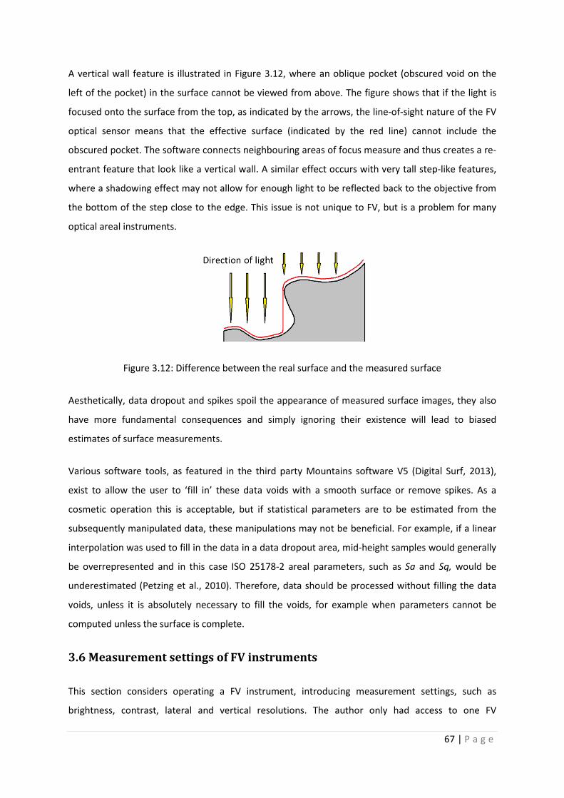
67 | P a g e
A vertical wall feature is illustrated in Figure 3.12, where an oblique pocket (obscured void on the
left of the pocket) in the surface cannot be viewed from above. The figure shows that if the light is
focused onto the surface from the top, as indicated by the arrows, the line-of-sight nature of the FV
optical sensor means that the effective surface (indicated by the red line) cannot include the
obscured pocket. The software connects neighbouring areas of focus measure and thus creates a re-
entrant feature that look like a vertical wall. A similar effect occurs with very tall step-like features,
where a shadowing effect may not allow for enough light to be reflected back to the objective from
the bottom of the step close to the edge. This issue is not unique to FV, but is a problem for many
optical areal instruments.
Figure 3.12: Difference between the real surface and the measured surface
Aesthetically, data dropout and spikes spoil the appearance of measured surface images, they also
have more fundamental consequences and simply ignoring their existence will lead to biased
estimates of surface measurements.
Various software tools, as featured in the third party Mountains software V5 (Digital Surf, 2013),
exist to allow the user to ‘fill in’ these data voids with a smooth surface or remove spikes. As a
cosmetic operation this is acceptable, but if statistical parameters are to be estimated from the
subsequently manipulated data, these manipulations may not be beneficial. For example, if a linear
interpolation was used to fill in the data in a data dropout area, mid-height samples would generally
be overrepresented and in this case ISO 25178-2 areal parameters, such as Sa and Sq, would be
underestimated (Petzing et al., 2010). Therefore, data should be processed without filling the data
voids, unless it is absolutely necessary to fill the voids, for example when parameters cannot be
computed unless the surface is complete.
3.6 Measurement settings of FV instruments
This section considers operating a FV instrument, introducing measurement settings, such as
brightness, contrast, lateral and vertical resolutions. The author only had access to one FV

68 | P a g e
instrument, the IFM G4, and therefore, this section heavily relies on the named instrument, in terms
of images and instrument specifications. Experiments investigating the effect of the settings on
measurements will be presented in Chapter 4, for which this section is important. Where
appropriate, a theoretical background will be given additionally, in order to explain the effect of the
settings.
3.6.1 Illumination
The FV technique works best when the object's surface is illuminated evenly. Most FV instruments,
however, only allow coaxial (through the objective) illumination, but it would be ideal if the surface
could be illuminated from all angles. To realise the latter, a dome of LED lights would have to be built
around the object. There are implications of such a setup: the object would have to be of small
dimensions to fit into the dome and as a result, the applicability of such a FV instrument would be
strongly restricted to small objects. Therefore, most FV instrument manufacturers limit the
illumination methods to coaxial light and ring-light. The ring-light is a circular collection of LED lights
mounted on to the objective lens, and it widens the light cone (defined by angle ϕ) shone on the
object's surface as shown in Figure 3.13(a).
The IFM G4 instrument can illuminate a workpiece with both sources: coaxial illumination and ring-
light illumination. The first source is used for most measurements and the latter is used particularly
when the surface is sloped. For measurements of surfaces with sloped and flat areas, the brightness
of both illumination sources must be balanced so that the flat surface is not overexposed.
Figure 3.13(b) shows a ring-light mounted to the 100× objective lens.
(a) (b)
Figure 3.13: (a) Illumination of ring-light, (b) ring-light attached to 100× lens on the IFM G4

69 | P a g e
In order to find a suitable brightness setting, the IFM G4 software offers a function that calculates
over- and underexposed areas and indicates these with two different colours in the live-view mode.
By varying the brightness level (or exposure time) the over- and under-exposed areas can be
controlled. When there is no indication of over- or under-exposed areas, best light setting for the
sample must be estimated. This subjectivity is a source of human error within the measurement
results. Horizontal surfaces are straight forward to measure because a level sample is rarely over-
and underexposed simultaneously and therefore, no trade-off is required. In contrast, a surface with
horizontal areas and steep slopes is difficult to measure because the balance between the over- and
underexposed areas is more difficult to find. The auto-exposure function can assist to establish good
illumination, but with the disadvantage of increasing measurement time and the loss of control over
measurement settings. In Figure 3.14 three surface representations are shown, which have been
acquired with different light settings: high exposure time (224 μs), medium exposure time (186 μs)
and low exposure time (112 μs). The images suggest that the high exposure cause spikes and that
the low exposure cause data holes in the surface.
(a) (b)
(c)
Figure 3.14: Surface measurements: (a) high, (b) low and (c) medium exposure times
3.6.2 Polariser
An ideal surface for the FV technique is one with a non-structured roughness. However, many
manufacturing processes, such as turning or honing, produce structured surfaces. Illumination of
these surfaces can result in localised specular (mirror-like) reflections leading to over- and
70 | P a g e
underexposed areas on the image plane. Tilted surfaces can also generate localised specular
reflections. In order to expand the FV technique’s applicability, polarisers can be inserted into the
optical path. A polariser filters light components that have a specific transverse propagation
orientation (Huard, 1997). With a polariser, the image quality improves but the exposure time is
elongated compared to the same measurement without a polarising filter or the illumination
intensity is increased.
3.6.3 Contrast
The contrast is a variable setting on the IFM G4 instrument. Unlike for the illumination there is no
automatic indication as to whether the contrast is too high or too low but it affects over- and under-
exposure: if the contrast is set too high, large singular areas of the image may be too bright or too
dark and the high spatial frequency change of brightness is lost and thus the information on the
degree of focus cannot be calculated. However, if the contrast is too low, there may be too little
contrast present for the detection of the surface. Finding the suitable contrast for a specific
measurement is subjective, similar to the brightness setting. In general, the contrast must be
adapted to every individual measurement to obtain high spatial frequency intensity changes (high
contrast) in each image of the image stack.
3.6.4 Lateral and vertical resolutions
In all versions of the IFM G4 software the vertical and lateral resolutions are variables for each of the
six objective lenses ranging from 2.5× to 100× magnification. The vertical and lateral resolutions
must be selected before the measurement because it has implications on the image processing.
Knowing the required resolution in advance is of benefit as computational time spent on image
processing can be saved.
The coarsest vertical resolution that can be selected on the IFM G4 is 132.76 µm (Table 3.1), which is
achievable with the 2.5× objective lens. With this large vertical resolution, however, a lot of
information between each object plane is not captured, which makes this setting unsuitable for
surface characterisation. The finest vertical resolution, (which for the IFM G4 is 10 nm), is achievable
with the 100× objective lens. A fine vertical resolution setting induces long measurement and
computational times because for a fixed scan height more images must be taken and processed
compared to a coarser vertical resolution.
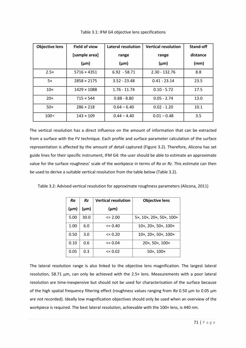
71 | P a g e
Table 3.1: IFM G4 objective lens specifications
Objective lens Field of view
[sample area]
(μm)
Lateral resolution
range
(μm)
Vertical resolution
range
(μm)
Stand-off
distance
(mm)
2.5× 5716 × 4351 6.92 - 58.71 2.30 - 132.76 8.8
5× 2858 × 2175 3.52 - 23.48 0.41 - 23.14 23.5
10× 1429 × 1088 1.76 - 11.74 0.10 - 5.72 17.5
20× 715 × 544 0.88 - 8.80 0.05 - 2.74 13.0
50× 286 × 218 0.64 – 6.40 0.02 - 1.20 10.1
100× 143 × 109 0.44 – 4.40 0.01 – 0.48 3.5
The vertical resolution has a direct influence on the amount of information that can be extracted
from a surface with the FV technique. Each profile and surface parameter calculation of the surface
representation is affected by the amount of detail captured (Figure 3.2). Therefore, Alicona has set
guide lines for their specific instrument, IFM G4: the user should be able to estimate an approximate
value for the surface roughness’ scale of the workpiece in terms of Ra or Rz. This estimate can then
be used to derive a suitable vertical resolution from the table below (Table 3.2).
Table 3.2: Advised vertical resolution for approximate roughness parameters (Alicona, 2011)
Ra
(μm)
Rz
(μm)
Vertical resolution
(μm)
Objective lens
5.00 30.0 <= 2.00 5×, 10×, 20×, 50×, 100×
1.00 6.0 <= 0.40 10×, 20×, 50×, 100×
0.50 3.0 <= 0.20 10×, 20×, 50×, 100×
0.10 0.6 <= 0.04 20×, 50×, 100×
0.05 0.3 <= 0.02 50×, 100×
The lateral resolution range is also linked to the objective lens magnification. The largest lateral
resolution, 58.71 µm, can only be achieved with the 2.5× lens. Measurements with a poor lateral
resolution are time-inexpensive but should not be used for characterisation of the surface because
of the high spatial frequency filtering effect (roughness values ranging from Ra 0.50 µm to 0.05 µm
are not recorded). Ideally low magnification objectives should only be used when an overview of the
workpiece is required. The best lateral resolution, achievable with the 100× lens, is 440 nm.

72 | P a g e
3.6.5 Objective Lenses
The IFM G4 has a turret on which six objectives lenses can be mounted. Alicona offers the following
six lens magnifications: 2.5×, 5×, 10×, 20×, 50×, and 100×. Customers are given comparable offers by
other FV instrument manufacturers; Zeta for example offers objective lenses with magnifications
between 2.5× and 150× (Zeta, 2013).
Not all FV instruments offer turrets for the mounting of the objective lenses as single mountings are
less costly. The stand-off distance (working distance) specifications of lenses vary too, therefore, not
any combination of objective lenses should be mounted on turrets. Turrets systems are usually
designed so that all lenses have their focal planes at a same distance from the image plane. The
danger of using turrets (see Figure 3.15) is the scratching of the lens, because some lenses have a
short working distance and these may come particularly close to the sample, especially the 100×
lens, which typically has a stand-off distance of 3 mm (see Table 3.1). In cases when samples have
raised surface features, the probability of coming into contact with the target surface is larger. The
100× objective lenses are the most expensive of all objective lenses on a typical FV instrument.
On FV instruments parfocal (focused on the same height) and parcentric (focused along the same
axis) lenses are standard. These lenses all focus to the same height, which means that when the
lenses are fitted to a lens turret, the object always stays in focus (or only requires minimal focal
adjustment), when switching from one lens to another. Thus, a small target can be found and
focused on to in a larger field of view and then zoomed into by changing the lenses to higher
magnifications. This helps to avoid accidental surface contact when changing lenses by rotating the
turret.
The choice of the objective lens magnification depends on the measurement task. The following
questions, which will be discussed, should serve as guidance to choosing an objective lens for a
measurement.
• How large is the projected surface area of interest?
• What resolution is necessary for the surface characterisation?
• What are the estimated surface characteristics?
• How large is the scan length?
• Does the surface include high aspect ratio areas?
• What is the time allowance for the measurement?

73 | P a g e
The three images in Figure 3.16 (a-c) demonstrate the effect of using different magnification lenses
to measure the same honed surface.
Figure 3.15: Parfocal objective lenses (2.5× to 100×) mounted on a turret
5716 µm × 4351 µm 1429 µm × 1088 µm 286 µm × 218 µm
(a) (b) (c)
Figure 3.16: Honed surface measured with (a) 2.5×, (b) 10× and (c) 50× objective lenses
How large is the projected surface area of interest? Each of the six objective lenses that can be used
for measurements on the IFM G4 have different field of views (FoV): the largest FoV is provided by
the 2.5× objective lens with dimensions of 5.7 mm × 4.4 mm, whilst the smallest FoV is 143 μm ×
109 μm when using the 100× objective lens (Table 3.1). The dimensions of other FoVs associated
with each lens are listed in Table 3.1. Ideally the feature of interest is captured within one FoV, or,
when using image stitching (see Figure 3.17), as few images as necessary, in order to minimise
measurement time; however it is not always feasible to have a specific FoV when also taking the
requirements for the lateral and vertical resolutions and the surface characteristics of the workpiece
into account.

74 | P a g e
Figure 3.17: Measurement using the image stitching function and four images
What resolution is necessary for the surface characterisation? The determination of the
measurement resolution depends on the information that is required from the object. For example,
if the waviness is in question, then the resolution may not have to be very high and thus a lower
objective lens can be used, however, if the object has a small roughness that is relevant for the
inspection, then a higher image resolution is required. The necessary resolution of the measurement
should be a known value before the measurement as it affects the measurement set-up.
Table 3.1 shows how the magnification of IFM G4's objective lenses is coupled with specific lateral
and vertical resolution bands: in general the higher the lens magnification is, the higher are the
obtainable resolutions. When comparing the measurement and image-processing times between
two measurements that differ only by the vertical resolution, the total time of the measurement
with the higher lateral resolution is longer.
What are the estimated surface characteristics? The surface roughness of a workpiece may not
always be of interest; it may be the waviness or the form instead. However, when the surface
roughness is of interest, it is good practice to estimate the roughness in terms of Ra or Rz using
comparative surface roughness scales, such as the Rubert scales, before setting up a measurement
with a FV instrument because the surface roughness dictates the range of vertical resolution that
should be used for its measurement.
How large is the scan height? The scan height is the distance covered by the moving optical system
in the Z axis, when recording images of the surface. The scan length is also equal to the difference in
the Z positions of the lowest and the highest image from one image stack (see Figure 3.2). For high
accuracy FV instruments, it is necessary that every area of interest on the sample surface passes
through the focal plane during scanning and that the scan starts and ends where the whole surface
is out of focus.

75 | P a g e
The scan length is theoretically limited by the stand-off distance of the objective lens, i.e. the scan
length cannot be equal or larger than the lens’ stand-off distance (Table 3.1) because the lens and
the workpiece would make contact when scanning the lower section.
If some pre-knowledge of the surface is present, or if multiple workpieces of the same shape and
size are measured, the scan length can be set by typing in the Z co-ordinates of the height markers.
The risk taken is missing data due to some features of interest lying outside the scanning range, or
wasting time due to unnecessarily long scan lengths. Figure 3.18 demonstrates in 2D were the
boundaries for the scan range must be set.
Figure 3.18: Setting the scan length
Does the surface include high aspect ratio areas? High aspect ratio surfaces are measured better
with higher magnification objective lenses because of the larger light cone that illuminates the
surface, which is described by the numerical aperture but at the cost of measurement time because
the resolution associated with a high magnification lens is higher. The implications of the numerical
aperture on the data collection of each image are demonstrated in Figure 3.19 but are explained
more in depth in Chapter 6 (analysis of high aspect ratio measurements).
Figure 3.19: High aspect ratio surface

76 | P a g e
What is the time allowance for the measurement? The influence on measurement time by each
setting (not only the objective lens) may have been hinted at in the previous paragraphs. Table 3.3
identifies all settings that affect measurement time negatively (increases). The table also states
which parts of the measurement time are increased: data-collection time or the computational time,
whereby the data-collection time is the time spent for data collection and the computational time is
spent on image processing and the construction of the measured surface.
Table 3.3: Effect of setting on time components
Settings Time-component
Long exposure time Data-collection time
Fine lateral resolution Computational time
Fine vertical resolution Data-collection time and computational time
Scan length Data-collection time and computational time
Number of areal sections (for stitching) Data-collection time and computational time
3.7 Summary
This chapter has been concerned with the development of the FV technique, the hardware and
software of current commercial FV instruments as illustrated by the Alicona IFM G4, the limitations
of the technique and the influence of settings on measurements.
The development of the FV technique started with Pentland (and Grossmann) who presented DOF,
where singular images were inspected for its PSF to determine the distance of an object from the
focal plane. Darell and Wohn's method of finding the DFF used an image stack and finding a focus
measure in each image by means of Gaussian and Laplacian pyramids. Nayar's method used image
stacks, similarly to Darell and Wohn, but the focus measure was calculated by a robust modified
Laplacian algorithm instead. Further developments of mathematical procedures for focus measure
calculations were pointed out.
The hardware components and the software tools of a commercial FV instrument have been
presented, the latter predominantly with a view towards post-processing of the effective surface in
order to obtain numerical values to describe surface characteristics. Instrument limitations have
been discussed in terms of the optics: some measurements cannot be conducted successfully due to
the surface's smoothness, or the angle of the surface, or the undulating nature of the surface.

77 | P a g e
The last section of this chapter presented the influences of settings on the outcome of a
measurement. This section is important for the set of experiments presented in subsequent
chapters, which will consider the capability of a FV instrument (IFM G4) for conducting experiments
that are designed to be at the limitation of the FV instrument capability.

78 | P a g e
Chapter 4: Instrument performance characteristics: measurement
noise
4.1 Introduction
Instrument performance characteristics are the information on the behaviour of an instrument
when applied to certain measurement tasks. Here the instrument performance characteristics in
terms of measurement noise are presented. The aim of this chapter is firstly to demonstrate a
method for assessing measurement noise of a FV instrument and secondly to explore the influence
each setting has on measurement noise. In the context of surface texture measurements these
assessments are very relevant: measurement noise affects the effective surface, which in turn
affects the calculation of surface texture parameters; and in the context of co-ordinate
measurements this assessment is equally relevant because measurement noise influences the
uncertainty, with which a shape can be fitted to an effective surface.
Noise measurement is formally defined as noise added to the output signal occurring during the
normal use of an instrument (ISO CD 25178-600, 2013). The random contribution is an error that
influences any profile or surface parameter calculated from the effective surface profile or area by
mathematical equations defined by the international working group ISO TC213-WG16 (ISO FDIS
25178-2, 2012).
The most familiar sources of noise for optical surface topography measurements are typically
classified as either hardware and software noise or environmental noise (Giusca, 2012). The first
source typically comprises electronic noise, which is a disturbance in the data transmission due to
electromagnetic interference (crosstalk) with neighbouring wires running in parallel, and also errors
due to data quantisation. Usually all wires are shielded to minimize this effect. Movable hardware
components, the optical head and the XY stage, are a source of vibration. These parts can be moved
using either at a fast or slow displacement speed. During measurements only the slow speed is used
in order to minimize the vibration and thus the noise level introduced to a measurement.
Environmental noise sources are independent of the measuring instrument. Environmental noise
sources comprise of ground vibrations and vibrations transmitted in air due to ventilation systems or
talking. The environmental sources of measurement noise are well known and well-equipped
metrology laboratories are typically temperature and humidity controlled to 20 °C ± 0.5 °C and 50 %
± 10 % rH.

79 | P a g e
In the context of this thesis, the definition of measurement noise will be broader than the official
definition given above: the measurement noise not only includes the sources of noise that were
mentioned above; but in this context includes ‘software induced noise’. Software induced noise here
means the noise added to the measurement by the error of focus measure calculation in each image
frame, as well as the measurement settings, such as exposure time and contrast, that make the
measurement less than optimal and prone to spikes or data loss.
In the case of the FV instrument IFM G4, a number of process settings must be considered for every
measurement. A range of variables is given for each setting, and therefore, a certain level of
familiarity of the measuring instrument is required in order to obtain good measurement results.
The deviation away from the optimal settings can be classified as human error, but will here be
referred to as ‘setting induced noise’ in order to distinguish it from the ‘overall noise’ (or general
noise).
The aim here was to discover the general noise, as defined in the draft ISO standard, and the setting
induced noise of the IFM G4. The general noise for each objective lens was assessed with a
mathematical procedure developed specifically for measurement noise assessment of profile surface
topography instruments (Haitjema, 2005), but transferable to optical instruments. The mathematical
details are given in the following section. The setting induced noise of the IFM G4 was assessed using
a comparative method: the noise level of a measurement completed with ‘good’ (mid-range)
settings was the comparator for measurements that only differed in one setting. The settings that
were varied are the following:
• exposure time (brightness),
• contrast,
• lateral resolution, and
• vertical resolution.
4.2 Calculating measurement noise
The noise of a surface measurement can be calculated using either of two methods. The first and
more straightforward noise measurement procedure is a subtraction method that is accepted for
noise assessment, and is documented in an official document by the Verband Deutscher Ingenieure
(VDI) (VDI/VDE 2655-1.1, 2008). The second is an addition (or averaging) method that has been
introduced by Haitjema (Haitjema, 2005).
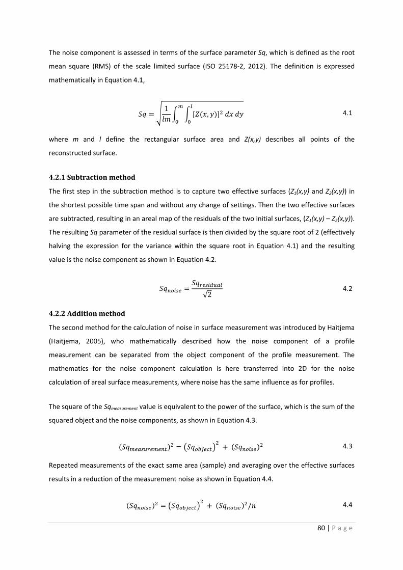
80 | P a g e
The noise component is assessed in terms of the surface parameter Sq, which is defined as the root
mean square (RMS) of the scale limited surface (ISO 25178-2, 2012). The definition is expressed
mathematically in Equation 4.1,
𝑆𝑆 = �1𝑙𝑙
� � [𝑍(𝑥,𝑦)]2 𝑑𝑥 𝑑𝑦𝑙
0
𝑚
0 4.1
where m and l define the rectangular surface area and Z(x,y) describes all points of the
reconstructed surface.
4.2.1 Subtraction method
The first step in the subtraction method is to capture two effective surfaces (Z1(x,y) and Z2(x,y)) in
the shortest possible time span and without any change of settings. Then the two effective surfaces
are subtracted, resulting in an areal map of the residuals of the two initial surfaces, (Z1(x,y) – Z2(x,y)).
The resulting Sq parameter of the residual surface is then divided by the square root of 2 (effectively
halving the expression for the variance within the square root in Equation 4.1) and the resulting
value is the noise component as shown in Equation 4.2.
𝑆𝑆𝑛𝑛𝑛𝑛𝑛 =𝑆𝑆𝑟𝑛𝑛𝑛𝑟𝑟𝑟𝑙
√2 4.2
4.2.2 Addition method
The second method for the calculation of noise in surface measurement was introduced by Haitjema
(Haitjema, 2005), who mathematically described how the noise component of a profile
measurement can be separated from the object component of the profile measurement. The
mathematics for the noise component calculation is here transferred into 2D for the noise
calculation of areal surface measurements, where noise has the same influence as for profiles.
The square of the Sqmeasurement value is equivalent to the power of the surface, which is the sum of the
squared object and the noise components, as shown in Equation 4.3.
(𝑆𝑆𝑚𝑛𝑟𝑛𝑟𝑟𝑛𝑚𝑛𝑛𝑚)2 = �𝑆𝑆𝑛𝑜𝑜𝑛𝑜𝑚�2 + (𝑆𝑆𝑛𝑛𝑛𝑛𝑛)2 4.3
Repeated measurements of the exact same area (sample) and averaging over the effective surfaces
results in a reduction of the measurement noise as shown in Equation 4.4.
(𝑆𝑆𝑛𝑛𝑛𝑛𝑛)2 = �𝑆𝑆𝑛𝑜𝑜𝑛𝑜𝑚�2 + (𝑆𝑆𝑛𝑛𝑛𝑛𝑛)2/𝑛 4.4

81 | P a g e
Where n is the number of repeated measurements. With the given information of the two equations
above, Equation 4.5 for noise can be derived,
(𝑆𝑆𝑛𝑛𝑛𝑛𝑛)2 = (𝑆𝑆𝑚𝑛𝑟𝑛𝑟𝑟𝑛𝑚𝑛𝑛𝑚)���������������������2 − (𝑆𝑆𝑚𝑛𝑟𝑛)2
1 − 𝑛−1 4.5
where (𝑆𝑆𝑚𝑛𝑟𝑛𝑟𝑟𝑛𝑚𝑛𝑛𝑚)���������������������2 is the mean of the measured values of Sq2.
The value for (Sqnoise)2 reaches a saturation value when an infinite number of images is used for the
evaluation of noise. Haitjema successfully demonstrated the applicability of this measurement noise
assessment technique with a Mitutoyo type SVC-624-3D roughness tester.
Giusca (Giusca, 2012) presented experimental results of noise measurements comparing the
subtraction method and the addition (averaging) method. One of the instruments used for the
comparison was a coherent scanning interferometer (with a 50× objective lens). For the noise
measurement a transparent glass flat was used and it was found that both noise measurement
techniques were successful for the areal measurements and that the difference between the results
was only a fraction of a nanometre when comparing four averaged measurements with four
subtractions of measurements.
4.3 Assessing measurement noise of the IFM G4
4.3.1 Method of assessing the effect of settings on noise
Previous research on measurement noise (Giusca, 2012) showed that both, the addition method and
the subtraction method, were successful for areal surface texture measuring instruments. In order to
perform the assessment of measurement noise of the IFM G4 FV instrument, the subtraction
method was chosen because it is the more time-efficient technique. Here the aim was to assess how
each individual setting influences the overall noise value, which can be achieved by comparing noise
measurements, using a reference noise measurement, for which the most appropriate (mid-range)
settings were used.
The subsequent measurements followed the same procedure with the same number of repeated
measurements (n), but with different settings: in order to separate the effect of a setting, only one
setting was changed from the mean value to the minimum or maximum of the setting’s range at a
time. For the ease of comparison, the reference values were normalized to 100 % and the other
values were matched accordingly.

82 | P a g e
The IFM G4 has six objective lenses; therefore, the complete comparative study was repeated for
each of the objective lenses, because the objective lenses have different associated vertical and
lateral resolution ranges (VR and LR, respectively) due to their differing magnifications. In Table 4.1,
the ranges for each of the settings in the IFM G4 software are given.
Table 4.1: Ranges of variable settings in the IFM G4 software
Setting Units Minimum Maximum
Exposure time (μs) 60 1,000,000
Contrast - 0.01 4.00
LR (2.5×) (μm) 6.92 58.71
LR (5×) (μm) 3.49 23.45
LR (10×) (μm) 1.75 11.74
LR (20×) (μm) 0.88 8.80
LR (50×) (μm) 0.64 6.40
LR (100×) (μm) 0.44 4.40
VR (2.5×) (μm) 2.30 132.50
VR (5×) (μm) 0.41 23.07
VR (10×) (μm) 0.10 5.71
VR (20×) (μm) 0.05 2.73
VR (50×) (μm) 0.02 1.19
VR (100×) (μm) 0.01 0.48
The artefact used for the assessment of noise on the IFM G4 was the wringing surface of a 4 mm
stainless steel gauge block that was roughened by a particle blasting method and supplied by Alicona
GmbH. The random roughness Ra was approximately 37 nm (measured with the Taylor Hobson PGI
1240, which had a resolution of 1.6 nm). The software used to post-process all surface
measurements was Mountains software V5 (developed by Digitalsurf). The measurements were
completed in a temperature (20 °C ± 0.5 °C) and humidity controlled environment (50 % ± 10 % rH).
For the assessment of the general noise measurement six surface measurements of the same area
(for sample sizes see Figure 3.1) were completed with the least possible time delay in between each
measurement and with no change of settings. The values for the two variable basic settings, the
exposure time and the contrast, were determined subjectively by the image displayed in the ‘live
view’ on the instrument’s computer screen. The exposure time was set so that the surface had no
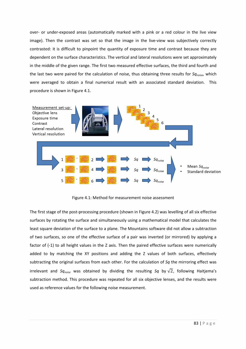
83 | P a g e
over- or under-exposed areas (automatically marked with a pink or a red colour in the live view
image). Then the contrast was set so that the image in the live-view was subjectively correctly
contrasted: it is difficult to pinpoint the quantity of exposure time and contrast because they are
dependent on the surface characteristics. The vertical and lateral resolutions were set approximately
in the middle of the given range. The first two measured effective surfaces, the third and fourth and
the last two were paired for the calculation of noise, thus obtaining three results for Sqnoise, which
were averaged to obtain a final numerical result with an associated standard deviation. This
procedure is shown in Figure 4.1.
Figure 4.1: Method for measurement noise assessment
The first stage of the post-processing procedure (shown in Figure 4.2) was levelling of all six effective
surfaces by rotating the surface and simultaneously using a mathematical model that calculates the
least square deviation of the surface to a plane. The Mountains software did not allow a subtraction
of two surfaces, so one of the effective surface of a pair was inverted (or mirrored) by applying a
factor of (-1) to all height values in the Z axis. Then the paired effective surfaces were numerically
added to by matching the XY positions and adding the Z values of both surfaces, effectively
subtracting the original surfaces from each other. For the calculation of Sq the mirroring effect was
irrelevant and Sqnoise was obtained by dividing the resulting Sq by √2, following Haitjema’s
subtraction method. This procedure was repeated for all six objective lenses, and the results were
used as reference values for the following noise measurement.

84 | P a g e
Figure 4.2: Method for measurement noise calculation
The same artefact was used for the setting induced noise measurements. For all six objective lenses,
the measurement and post-processing procedures were performed with only one differing setting
compared to the reference set of settings. The changed setting was at either towards the minimum
or towards the maximum limit of the setting’s range. Table 4.2 gives the explanation to the codes
used in Tables 4.3 to 4.8, which present the numerical values of the settings for each lens
magnification.
The different lateral and vertical resolution ranges and numerical apertures of each objective lens
make inter-comparisons of measurements performed with different objective lens magnification
difficult. For example, the 100× lens has a finer vertical and lateral resolution than the 50× lens, and
a larger numerical aperture, which gives it the ability to collect a wider angle of backscattered light
and therefore, more information. Therefore, in order to inter-compare between results of different
optical lenses, the comparative study was based on percentage of noise increase or decrease from
the reference.

85 | P a g e
Table 4.2: Key to setting codes
Setting codes Meaning of code
R Reference
LExp Low Exposure time
HExp High Exposure time
LC Low contrast
HC High contrast
LLRes Low (coarse) lateral resolution
HLRes High (fine) lateral resolution
LVRes Low (coarse) vertical resolution
HVRes High (fine) vertical resolution
Table 4.3: Combinations of settings for the 2.5× lens
Lens magnifi-
cation Setting codes
Exposure
time
(μs)
Contrast
Vertical
resolution
(μm)
Lateral
resolution
(μm)
2.5×
R 153 1.39 15.78 20.00
LExp 99 1.39 15.78 20.00
HExp 235 1.39 15.78 20.00
LC 153 0.11 15.78 20.00
HC 153 1.96 15.78 20.00
HVRes 153 1.39 2.37 20.00
LVRes 153 1.39 61.81 20.00
HLRes 153 1.39 15.78 9.00
LLRes 153 1.39 15.78 58.71

86 | P a g e
Table 4.4: Combinations of settings for the 5× lens
Lens magnifi-
cation Setting codes
Exposure
time
(μs)
Contrast
Vertical
resolution
(μm)
Lateral
resolution
(μm)
5×
R 172 1.93 2.69 7.82
LExp 112 1.93 2.69 7.82
HExp 224 1.93 2.69 7.82
LC 172 0.11 2.69 7.82
HC 172 1.95 2.69 7.82
HVRes 172 1.93 0.41 7.82
LVRes 172 1.93 10.97 7.82
HLRes 172 1.93 2.69 3.73
LLRes 172 1.93 2.69 23.48
Table 4.5: Combinations of settings for the 10× lens
Lens magnifi-
cation Setting codes
Exposure
time
(μs)
Contrast
Vertical
resolution
(μm)
Lateral
resolution
(μm)
10×
R 153 1.61 0.47 5.66
LExp 112 1.61 0.47 5.66
HExp 244 1.61 0.47 5.66
LC 153 0.15 0.47 5.66
HC 153 4.00 0.47 5.66
HVRes 153 1.61 0.10 5.66
LVRes 153 1.61 2.76 5.66
HLRes 153 1.61 0.47 1.85
LLRes 153 1.61 0.47 11.74

87 | P a g e
Table 4.6: Combinations of settings for the 20× lens
Lens magnifi-
cation Setting codes
Exposure
time
(μs)
Contrast
Vertical
resolution
(μm)
Lateral
resolution
(μm)
20×
R 235 1.72 0.19 2.93
LExp 116 1.72 0.19 2.93
HExp 309 1.72 0.19 2.93
LC 235 0.01 0.19 2.93
HC 235 4.00 0.19 2.93
HVRes 235 1.72 0.05 2.93
LVRes 235 1.72 1.29 2.93
HLRes 235 1.72 0.19 1.37
LLRes 235 1.72 0.19 7.96
Table 4.7: Combinations of settings for the 50× lens
Lens
magnifi-
cation
Setting codes Exposure time
(μs) Contrast
Vertical
resolution
(μm)
Lateral
resolution
(μm)
50×
R 577 2.03 0.08 2.13
LExp 297 2.03 0.08 2.13
HExp 922 2.03 0.08 2.13
LC 577 0.01 0.08 2.13
HC 577 4.00 0.08 2.13
HVRes 577 2.03 0.02 2.13
LVRes 577 2.03 0.52 2.13
HLRes 577 2.03 0.08 0.99
LLRes 577 2.03 0.08 3.17

88 | P a g e
Table 4.8: Combinations of settings for the 100× lens
Lens
magnifi-
cation
Setting codes Exposure time
(μs) Contrast
Vertical
resolution
(μm)
Lateral
resolution
(μm)
100×
R 1040 1.76 0.03 1.10
LExp 474 1.76 0.03 1.10
HExp 2010 1.76 0.03 1.10
LC 1040 0.01 0.03 1.10
HC 1040 4.00 0.03 1.10
HVRes 1040 1.76 0.01 1.10
LVRes 1040 1.76 0.22 1.10
HLRes 1040 1.76 0.03 0.70
LLRes 1040 1.76 0.03 1.58
4.3.2 Results and discussion
The results obtained from all of the noise measurements are organised as follows: the reference
noise measurements of all lenses are presented first, then all the results are grouped according to
the magnification lens of each measurement, then the results are reorganised into the each setting
variable (exposure time, contrast etc.) in order to discuss a different aspect of the results, and lastly
the results of all lenses are combined to obtain a graph that presents a summary of the results for
each type of setting.
4.3.2.1 Reference values
Numerical values for the reference noise measurements (with mid-ranged settings) with all six
lenses are presented in Figure 4.3, where the noise value has been plotted against the magnification
of the objective lens used for each measurement. Each value is accompanied by an error bar that
shows ± 1 σ (standard deviation) of the repeated measurements. The trend of the noise
measurements could be approximated by a decreasing exponential function: the noise measured
with the 2.5× objective lens had the highest Sqnoise value of 565.7 nm, whilst the 5× lens noise
measurement gave a result of 169.5 nm, followed by 39.8 nm, 14.4 nm, 5.9 nm and 3.1 nm,
respectively for the 10×, 20×, 50×, and 100× objective lenses. The associated standard deviations
(although not always visible in the graph and, therefore, tabulated in Table 4.9) reflect the

89 | P a g e
exponentially decreasing trend of the noise values: the standard deviations decrease from 26.1 nm
to 0.4 nm with respective lens magnifications increasing from 2.5× to 100×.
Figure 4.3: Reference measurement noise (± 1 σ) of all lenses
Table 4.9: Reference measurement noise data
Lens magnification Meas. noise
(nm)
Standard deviation
(nm)
2.5× 565.7 26.1
5× 169.5 10.4
10× 39.8 2.9
20× 14.4 0.4
50× 5.9 0.4
100× 3.1 0.4
4.3.2.2 Setting induced measurement noise for each lens
The numerical results of the setting induced noise measurements are presented in terms of
percentage of the reference noise measurement result in order to make them comparable across all
lenses. Two observations of the results presented in Figures 4.4 to 4.9 are as follows:
2.5
5
10 20 50 100 0
100
200
300
400
500
600
0 20 40 60 80 100
Sqno
ise /
nm
Lens magnification

90 | P a g e
• measurement settings influence measurement noise, and
• each setting affects measurement noise differently.
Measured noise components showed a similar pattern when comparing the noise results of one lens
magnification to another lens magnification. One can observe that a short exposure time induced
more noise into the effective surface, whilst a long exposure time generally reduced the noise
component. Similarly one can observe that a low lateral resolution reduced the amount of noise in a
measurement and a high lateral resolution resulted in a higher measurement noise than the
reference. In contrast to the lateral resolution, the variation of the vertical resolution reduced the
noise component when the vertical resolution was high and increased the noise component when
the vertical resolution was low. Concerning the contrast, the results showed that in most cases the
influence was small (within ± 10 % of the reference value). Table 4.10 summarises the manner in
which a setting affected the measurement noise.
Figure 4.4: Measurement noise for the 2.5× lens and different settings (± 1 σ)
Figure 4.5: Measurement noise for the 5× lens and different settings (± 1 σ)
100%
149%
65% 107% 101%
43%
109% 132%
43%
0%
50%
100%
150%
200%
250%
300%
R LExp HExp LC HC LLRes HLRes LVRes HVRes
Rela
tive
nois
e /
%
Setting
100%
173%
109% 116% 110%
48%
152% 115%
49%
0%
50%
100%
150%
200%
250%
300%
R LExp HExp LC HC LLRes HLRes LVRes HVRes
Rela
tive
nois
e /
%
Setting

91 | P a g e
Figure 4.6: Measurement noise for the 10× lens and different settings (± 1 σ)
Figure 4.7: Measurement noise for the 20× lens and different settings (± 1 σ)
Figure 4.8: Measurement noise for the 50× lens and different settings (± 1 σ)
100% 141%
73% 89% 98%
49%
176%
392%
91%
0%
50%
100%
150%
200%
250%
300%
350%
400%
450%
500%
R LExp HExp LC HC LLRes HLRes LVRes HVRes
Rela
tive
nois
e /
%
Setting
100%
281%
85% 68% 58% 38%
143%
198%
52%
0%
50%
100%
150%
200%
250%
300%
R LExp HExp LC HC LLRes HLRes LVRes HVRes
Rela
tive
nois
e /
%
Settings
100%
186%
73% 92% 94%
62%
146% 155%
57%
0%
50%
100%
150%
200%
250%
300%
R LExp HExp LC HC LLRes HLRes LVRes HVRes
Rela
tive
nois
e /
%
Setting

92 | P a g e
Figure 4.9: Measurement noise for the 100× lens and different settings (± 1 σ)
Table 4.10: Summary of the effect of settings
Setting Effect on measurement noise
Low exposure time,
High lateral resolution,
Low vertical resolution
Increase
High exposure time,
Low lateral resolution,
High vertical resolution
Decrease
Contrast Insignificant change
4.3.2.3 Results organised by setting
The results have been re-organised here in order to see more clearly if the effect of a particular
setting on the measurement noise correlates with the magnification of the objective lens used.
Figures 4.10 to 4.13 present the re-organised measurement noise values, excluding the reference
values that have already been inspected separately. Despite some outliers, the outcome of the re-
organised data can be summarised as follows: there was no correlation between the relative
percentage of measurement noise of one particular setting and the lens magnification. This
observation may be a result of the different ratios between the reference values and the changed
setting value. So far the measurement noise was only described in terms of positive and negative
influence, which corresponded to values above and below the reference value. Here the
presentation of the results will be quantified.
100%
196%
64% 87%
109% 95%
150% 157%
96%
0%
50%
100%
150%
200%
250%
300%
R LExp HExp LC HC LLRes HLRes LVRes HVRes
Rela
tive
nois
e /
%
Settings

93 | P a g e
Exposure time
When a low exposure time was set for the repeated measurements for the noise test, then, for all
lenses, the noise was larger than the reference value, with 149 %, 173 %, 141 %, 281 %, 186 %, and
196 % for all six lenses (in order of increasing magnification). Increasing the exposure time to the
instrument's limit resulted generally in a smaller noise level, with 65 %, 109 %, 75 %, 85 %, 73 %, and
64 %, respectively for all six lenses from 2.5× to 100×. Of these values, one outlier was observed in
the data for short exposure time (281 %) of the 20× magnification lens.
Figure 4.10: Measurement noise as a function of low and high exposure time settings (± 1 σ)
Contrast
The inspection of how contrast setting affects measurement noise did not show a clear positive or
negative indication. Instead it was found that the noise values of both high and low contrast
measurements with all objective lenses are scattered in the proximity of the 100 % mark of the
reference value. The noise results for the low contrast measurements were 107 %, 116 %, 89 %,
68 %, 92 %, and 87 % for all lenses in order of increasing magnification. Presented in the same
manner, the results of measurements with high contrast were 101 %, 110 %, 98 %, 58 %, 94 %, and
109 %, respectively.
149% 173%
141%
281%
186% 196%
65%
109%
73% 85% 73% 64%
0%
50%
100%
150%
200%
250%
300%
2.5x 5x 10x 20x 50x 100x
Rela
tive
nois
e /
%
Lens magnification
low exposure time
high exposure time

94 | P a g e
Figure 4.11: Measurement noise as a function of low and high contrast settings (± 1 σ)
Lateral resolution
The relative noise values for the measurements with a low lateral resolution setting were 43 %, 48
%, 49 %, 38 %, 62 %, and 95 %, for all lenses from 2.5× to 100×, respectively. And similarly for the
high lateral resolution measurements, the relative noise values were 109 %, 152 %, 176 %, 143 %,
146 %, and 150 %.
Figure 4.12: Measurement noise as a function of low and high lateral resolution settings (± 1 σ)
107% 116% 89%
68% 92% 87%
101% 110% 98%
58%
94% 109%
0%
50%
100%
150%
200%
250%
300%
2.5x 5x 10x 20x 50x 100x
Rela
tive
nois
e /
%
Lens magnification
low contrast
high contrast
43% 48% 49% 38% 62%
95% 109%
152% 176%
143% 146% 150%
0%
50%
100%
150%
200%
250%
300%
2.5x 5x 10x 20x 50x 100x
Rela
tive
nois
e /
%
Lens magnification
low lateral resolution
high lateral resolution

95 | P a g e
Vertical resolution
In general the extreme vertical resolution setting had the opposite effect on measurement noise
compared to the extreme lateral resolution settings: a low vertical resolution worsened the
measurement noise (132 %, 115 %, 392 %, 192 %, 155 %, and 149 % for all lenses from 2.5× to 100×)
and a high vertical resolution improved the measurement noise (43 %, 49 %, 91 %, 52 %, 57 %, and
63 %, respectively).
Figure 4.13: Measurement noise as a function of low and high vertical resolution settings (± 1 σ)
4.3.2.4 Results across all lenses
It was seen that the relative measurement noise did not correlate with the objective lens
magnification, therefore, in the following sub-section the results are organised in such a way that
shows the mean of all results (in terms of percentage) of each setting categories. Note again that
these results are representative only for this particular experimental setup and can be viewed as
trends on a more general level. Figure 4.14 presents the influence of each setting whilst disregarding
the lens magnification. The range of standard deviations (1 σ) was large, ranging from 17 % to 113 %.
The largest measurement noise deviation for each setting was mainly due to one outlying value,
except in the case for low lateral resolution where there were two outlying values.
Outlying values were defined as those values that were not within one standard deviation range
from the mean, as highlighted in the preceding section. If the mean of noise components measured
132% 115%
392%
198% 155% 157%
43% 49% 91%
52% 57% 96%
0%
50%
100%
150%
200%
250%
300%
350%
400%
450%
500%
2.5x 5x 10x 20x 50x 100x
Rela
tive
nois
e /
%
Lens magnification
low vertical resolution
high vertical resolution

96 | P a g e
with all six objective lenses was calculated without the outlying values, then relative noise
components did not shift significantly but the standard deviation was reduced significantly, so that
the largest standard deviation was not larger than 48 %. The following statements can be developed
as a function of assessing the data in the summarising graph (Figure 4.14):
• Very low vertical resolution influenced the noise component most (increase of 98 %),
followed by a short exposure time (increase of 88 %).
• The low and high lateral resolutions influenced the noise strongly causing the noise to
decrease by 44 % and increase by 46 %, respectively.
• On average, the contrast did not introduce a change of noise level larger than 10 % of the
noise expected for ‘good’ (reference) settings.
Figure 4.14: Relative mean measurement noise of all lenses (± 1σ)
4.3.3 Discussion and conclusions
The conclusion drawn from these observations was that measurements of higher magnification
lenses were less prone to noise. This trend matched expectations of the noise measurements, which
were rooted in the fact that higher lens magnifications measure a much smaller field of view and
therefore not as much noise is represented. However, this conclusion must be considered with
caution because although the results have indicated that the combination of settings influences the
measurement noise component (assuming that environmental disturbances influenced each
measurement equally) the effect of the measuring task has not yet been considered and may give
rise to another reason for increased noise levels for low magnification lenses compared to high
magnification lenses. The reason may be linked to improper overlapping of images when subtracting
two images within the Digitalsurf Mountains V5 software environment.
100%
188%
78% 93% 95% 56%
146%
198%
58%
0%
50%
100%
150%
200%
250%
300%
350%
R LExp Hexp LC HC LLRes HLRes LVRes HVRes
Mea
n re
lativ
e no
ise
/ %
Settings
Average of all lenses
97 | P a g e
The measurement task was repeated measurements of one artefact (the roughened gauge block),
which was the same for all lenses. There are two consequences of this measurement task. Firstly,
images obtained with low magnification lenses (for example the 2.5× lens, which naturally has a low
lateral resolution) contain less high spatial frequency information than images taken of the same
surface but with a higher magnification lens (for example the 100× objective with a high resolution).
Secondly, in a camera set-up with a low magnification lens, each pixel images a larger surface area
than a pixel in a camera set-up with a higher magnification lens.
If the second image differs from the first by a lateral shift of one pixel, then the images do not
overlap or correlate properly when subtracting the images in the post-processing step. This has a
more significant consequence for images obtained with a low magnification lens because the shift is
larger than for images with a high magnification lens. As a result, the residual of a subtraction
procedure is larger for images taken with low magnification lenses than images taken with large
magnification lenses.
The exposure time had a very well-defined effect on measurement noise. Long exposure time
settings resulted in low measurement noise as a consequence of integration of noise, and as a result
the measurements with short exposure times were not as repeatable as the measurements with long
exposure times. The resulting effective surfaces with the short exposure time setting may have
contained more defects such as spikes or data gaps.
The measurement noise test with extreme contrast settings showed results that were against
expectations: it was expected that high contrast images would have a lower noise level than low
contrast images because the FV technique relies on highly contrasted images. A possible explanation
for this result may be the roughness of the surface that was already very well suited for the
instrument, so that any changes of the contrast setting did not affect the measurement in any
particular way.
A low lateral resolution effectively acts as a high spatial frequency filter during the capture of the
effective surface; therefore, the effective surface can be represented in a smoother manner than the
real surface, when there is no influence of high spatial frequency aliasing (Mauch, 2012). It was
mentioned above that most noise components have high spatial frequencies, which are eliminated
by the low lateral resolution. A high lateral resolution should, therefore, be associated with a high
noise component, and this was reflected in the measurement results. For the vertical resolution one
would expect the opposite effect on the effective surface because a courser vertical resolution does
not cause a filtering effect, instead it leaves too large gaps between captured data on a steep surface

98 | P a g e
and this causes noise. The results showed this expected behaviour: the coarse vertical resolution
setting was associated with a high measurement noise and vice versa for a fine vertical resolution
setting.
In summary, this novel investigation of measurement noise fulfilled the aim to understand the
influence of basic instrument settings of the FV instrument, the IFM G4, on the noise components of
the effective surface and the following conclusions were drawn from the results. It is necessary to
bear in mind that these results are specific only to these particular measurement settings. Because
of the lack of an absolute reference mark, only the generic trends that these results show can be
generalised.
• Measurement noise was linked with the magnification of the objective lenses: the larger the
magnification was, the smaller the noise component was.
• Significant negative influences of settings on measurement noise were low vertical
resolution (increase of 98 %), short exposure time (increase of 88 %), and high lateral
resolution (increase of 46 %).
• Significant positive influences of settings on measurement noise were, a low lateral
resolution (decrease of 44 %), a high vertical resolution (decrease of 42 %), and a long
exposure time (decrease of 22 %).
• The image contrast did not influence measurement noise significantly.

99 | P a g e
Chapter 5: Instrument performance characteristics: residual flatness
5.1 Introduction
Key areal instrument characteristics that affect positional information of every measurement
systematically are residual flatness. This part of the research investigates different methods for the
measurement of residual flatness on a FV instrument, which are tested with the IFM G4.
The definition of residual flatness is the “flatness of the areal reference” (ISO CD 25178-600, 2013).
For a better understanding of residual flatness, one can refer to the definition of geometric flatness,
which is the separating distance of two virtual parallel planes bracketing a surface, in between which
all measured points are confined (ISO 1101, 2012). For any surface topography optical instrument,
residual flatness, as opposed to measurement noise, is a systematic error introduced into every
measurement by the general form of the objective lenses, scratches on objective lenses, the CCD
camera, and misalignments in the optical system.
If one was to measure a perfect optically flat object with an areal surface topography instrument,
then any deviation from the effective surface’s mean plane may be designated as a fault of noise or
residual flatness of the instrument. Practically this is not feasible due to manufacturing imperfections
when realising an optical flat, and therefore, different methods have to be used to assess residual
flatness of any particular instrument.
In the previous chapter it was shown how the measurement noise could be measured. Here the aim
is to measure the flatness separately from the noise. In contrast to measurement noise, the
instrument’s residual flatness term is typically dominated by low spatial frequency noise components
due to influences such as imperfect curvature of lens elements or a slightly curved imaging plane.
High spatial frequency residual flatness components are usually due to scratches on the lenses as a
result of imprudent handling of the objective lens.
Unlike for surface texture measurements, where the instrument's residual flatness has the same
effect on each individual surface measurement, for dimensional measurements, the effect of residual
flatness differs for each measurement. Here are two examples, which should help to understand how
the residual flatness affects dimensional measurements differently. The first example is a
measurement of a step height using two points within one FoV, and only the vertical difference
between the points is important. For simplicity it is assumed that one data point of the point cloud is
chosen to represent a point on a surface, assuming that the surface is not affected by spikes. The

100 | P a g e
point chosen on the upper surface happens to be in approximately the centre of the FoV, and the
lower point is towards the boundary of the FoV and the height difference is calculated. If the residual
flatness affects the measurement height map spherically and the residual flatness error at the centre
is largest (in the positive Z direction), then the height difference between the two points is
overestimated.
The second example is a sphere measurement whereby the FoV centre is aligned with the top of the
sphere. If the residual flatness error affects the measurement height map in the same way as in the
previous example, then the effective surface has a larger curvature than the object and as a result a
the radius is underestimated and the centre of the sphere is calculated to be at a higher position
than the measurand.
5.2 Measuring residual flatness of areal surface texture measuring
instruments
Previous work on the assessment of residual flatness for surface topography instruments has been
presented by the NPL, where Giusca (Giusca, 2012) has characterised the flatness of three different
types of surface measuring instruments: a contact stylus instrument, a coherence scanning
interferometer (CSI) and an imaging confocal microscope (ICM). For the study, Giusca consistently
used a method which was based on prior work by the German VDI/VDE committee (VDI/VDE 2655,
2008; Giusca and Leach, 2013b; Giusca and Leach, 2013c).
On the basis of two assumptions, Giusca at the NPL developed an averaging method: the first
assumption was that the noise component of the error term was random and the flatness term was
systematic; and the second assumption was that the optical flat was imperfect. The method used an
averaging technique: ten measurements of a flat reference artefact were carried out at different
locations on the flat surface in order to account for localised imperfections in the reference flat (i.e.
scratches). The images were then numerically summed, whereby the height (Z) values of the
effective surfaces were summed on a point to point basis, as shown in Equation 5.1, where the
expression in the bracket is Sz. The measurement method is shown in Figure 5.1.
𝑆𝑆𝑓𝑙𝑟𝑚𝑛𝑛𝑛𝑛(𝑥,𝑦) = ��𝑍𝑛(𝑥,𝑦)𝑛
𝑛=1
�1𝑛
5.1

101 | P a g e
Figure 5.1: Residual flatness measurement method
The flatness is expressed as the resulting maximum height of the scale limited surface, Sz, value
divided by the number of images. The surface parameter, Sz, is defined as the “sum of the largest
peak height value and the largest pit depth values within a defined area” (ISO 25178-2, 2012). An
implication of the averaging technique is a stabilisation of residual flatness value Szflatness when a large
the number of effective surfaces are used. The averaging method for residual flatness error
assessment is designed to leave any systematic roughness, waviness and form terms in each
individual image unfiltered, but the noise component as well as the random height variations of the
surface should also be minimised by the averaging process.
Giusca presented the results of residual flatness measurements using this averaging technique for
the CSI and the ICM. Both measurement techniques are capable of measuring optically flat surfaces,
and therefore, an optical flat was used for the test. Results of both instruments showed that not
more than ten effective surfaces were required for the residual flatness value Sz to stabilise (Giusca,
2012).
5.3 Measuring residual flatness of a FV instrument
The averaging method for residual flatness measurements of more common areal instruments, such
as the CSI, has been laid out. The requirement for a successful residual flatness assessment with that
method was the instrument’s ability to measure optically flat surfaces. FV instruments are not
capable of measuring an optical flat due to the requirement of a minimum roughness specification
and are, therefore, excluded from the application of this residual flatness measurement method.
Therefore, a variation of this averaging method was required in order to make it applicable to FV
instruments. An averaging method could be applied to FV instruments if the optical flat was replaced
by a roughened flat surface with a Ra of approximately 30 nm roughness. The roughened flat was not
allowed to have a form with a special frequency similar to the image size. In the following, three
variations of averaging methods are presented. The aim here was to investigate how well these three

102 | P a g e
methods worked for FV instruments and to assess these in the context of acceptance and re-
verification tests, and health checks. It should be noted that this work is unique in the context of FV.
Experiments or results on the residual flatness of the IFM G4 have not been previously published,
which makes this investigation a novelty. Consequently a comparator for the results was not
available. However, the averaging methods implied that the averaged residual flatness value, Szflatness,
should converge to the true residual flatness value by decaying to a minimum, which is smaller than
the Sz values of the effective surfaces. Based on that implication, it was assumed for each residual
flatness method that the smaller the Szflatness value was, the closer the value was to the true residual
flatness value.
Only four of the six available objective lenses of the IFM G4 were inspected for residual flatness, with
magnifications 10×, 20×, 50× and 100× (see Table 3.1 for FoVs), because these are the main lenses
used for surface texture measurements. The flat reference artefact used for all twelve investigations
(all three methods applied to all four lenses) was a wringing surface of a gauge block, which was
roughened by means of particle blasting. The roughened surface was inhomogeneous (random) in
nature and had a roughness (Ra) of 37 nm (measured with the Taylor Hobson PGI 1240, which had a
resolution of 1.6 nm). Although the averaging method would theoretically converge to the true
flatness value with fewer measurements, the artefact's roughness was necessary to ensure good
image quality. All data processed was completed using the Mountains software V5. All
measurements were completed in a temperature and humidity controlled environment at 20 ˚C ±
0.5 ˚C and 50 % ± 10 % rH, respectively.
5.3.1 Ten image method
The first averaging method for FV instruments using ten measurements and a roughened artefact will
be referred to as the ‘10i-method’, where the “i” stands for ‘image’ (equivalent to effective surface).
In principle this method followed the same procedure as presented by Giusca but with a roughened
flat instead of an optical flat.
Ten measurements were performed at different locations on the above specified roughened flat. All
measurements were imported into the Mountains software and levelled by rotation using a least
squares fit method. The levelling ensured that long wavelength components (four times larger than
the measurement frame width) of the imperfect flat artefact were not included in the residual
flatness measurement.

103 | P a g e
Some images would contain ‘volumeless’ spikes, which are a consequence of measurement noise:
they are created during the realisation of the effective surface when one outlier is not recognised as
such and is connected to the data cloud that represents the rest of the effective surface (see
Figure 5.2). The truncation of ‘volumeless’ spikes was part of the method and occurred after the
levelling of all measurements. Truncation of ‘volumeless’ spikes was realised by applying a horizontal
(DC) threshold to each of the ten levelled measurements (effectively filtering the image data set with
an upper and lower height limit).
Figure 5.2: ‘Volumeless’ spike
All levelled measurements were then numerically added together on a pixel by pixel basis as
described above, which averaged out the random components such as measurement noise (the
randomly added height variations that contain volume) as well as the roughness. When the surface
measurements were added together, the chances that peaks and valleys of the roughness cancelled
each other out was high, thus minimising the artefact’s surface texture and isolating the systematic
residual flatness from the noise. Finally, the Sz parameter was calculated from the resulting height
map and divided by the number of measurements (10) in order to obtain the quantified information
about the instrument's residual flatness (Szflatness). The measurement method for FV instruments is
shown in Figure 5.3.
Figure 5.3: Flowchart of residual flatness measurement procedure for the IFM G4

104 | P a g e
5.3.2 Ten image with filter method
The second method, called the ‘10if-method’, differed from the 10i-method by the addition of a
waviness filters, with cut-off values of 800 μm for the 10× lens, 250 μm for the 20× lens, and 80 μm,
for the 50× and 100× lenses. The cut-off wavelength values were chosen according to the lens
magnification because measurements performed with higher lens magnifications have smaller
measurement frame widths. These filters eliminated short wavelength information from the
resulting height map, and were applied to the sum of the ten surface measurements with the effect
of isolating the underlying signal components that contribute directly to the Szflatness value.
5.3.3 Hundred image method
The third averaging method differed from the ‘10i-method’ by the number of measurements, 100,
used for the assessment. This more rigorous residual flatness measurement method was referred to
as the ‘100i-method’. The execution of the image post-processing was almost identical to the image
post-processing for the 10i-method (see Figure 5.3). Only the data collection (measurements)
method differed from the 10i-method because here an image field containing 100 single
measurements was measured and all single measurements saved separately. Each of the individual
measurements overlapped with the neighbouring measurement by only 10 %, and therefore, the
form error should have been left unfiltered, and the random error should have been removed by the
averaging technique.
5.3.4 Experimental results
The presentation of the experimental results is organised similarly to the measurement noise's
results in Chapter 4. Qualitative impression of all results is given first, followed by a quantitative
presentation of all results. The final levelled and summed images from the three methods using the
10×, 20×, 50× and 100× objective lenses are shown in Figures 5.4 to 5.7. Note that the images shown
in the named figures are screenshots from the final page of the processing stage in the Mountains
software and that, therefore, the Sz values are not the Szflatness values.
Qualitatively the final summed images of all three methods compared similarly for lens
magnifications. In general it was observed that the final image of the 10i-method did not show a
distinctive form error, and instead many peaks and valleys were strongly present, which were
assumed to be elements of the artefact’s surface texture. Visually, this high spatial frequency
component was dominant and its height difference affected the overall Sz parameter. The result of
the 10if-method showed so that the high spatial frequency roughness component was eliminated

105 | P a g e
and the form error (or residual flatness component) was visible. The resulting image of the 100i-
method included visible high spatial frequency peaks and valleys, similarly to the result of the 10i-
method, but with the difference that the height variation of the high spatial frequency component
did not dominate over the form component. The residual flatness error generated by the 100i-
method was comparable in shape to the residual flatness error generated by the 10if-method.
A qualitative comparison between the summed images obtained with each method showed that
objective lenses with lower magnifications did not show the above trends as clearly as the results of
the 100× objective lens, suggesting that the number of images for lower magnification lenses must
be increased.

106 | P a g e
Figure 5.4: Summed images for the 10× lens
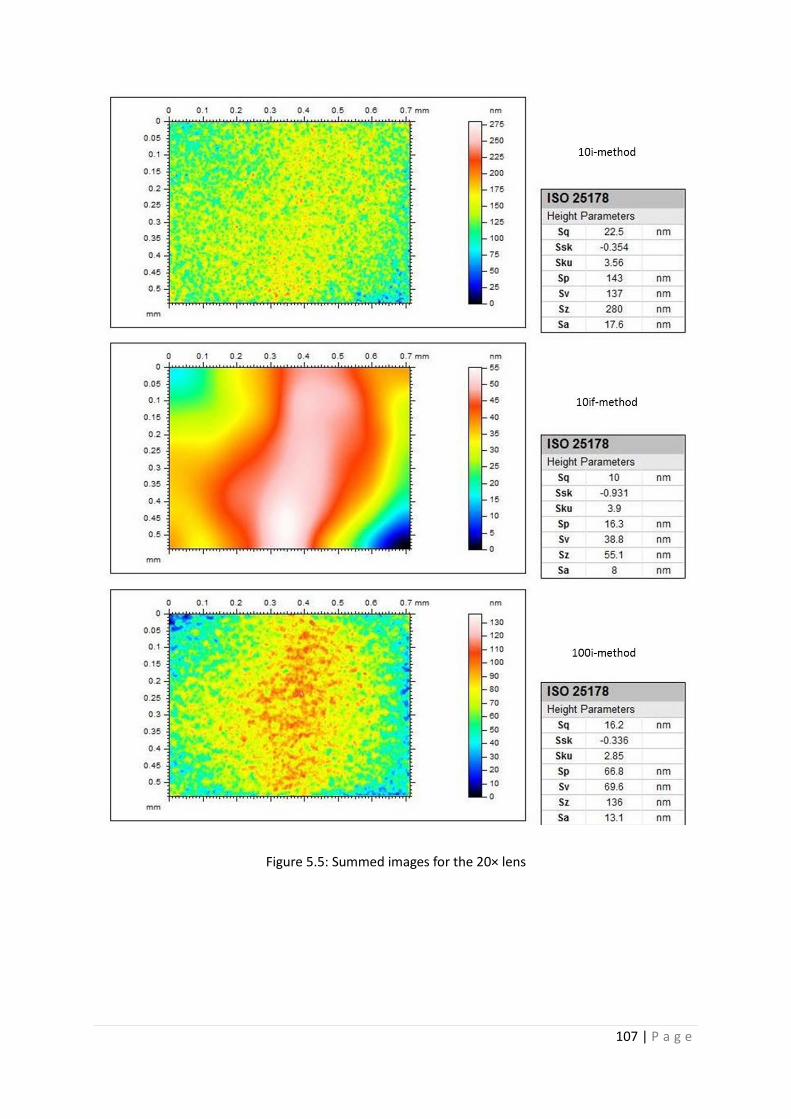
107 | P a g e
Figure 5.5: Summed images for the 20× lens

108 | P a g e
Figure 5.6: Summed images for the 50× lens

109 | P a g e
Figure 5.7: Summed images for the 100× lens
The numerical results were coherent with the conclusions drawn from the visual appearance of the
final residual flatness error images, and are presented in Table 5.1, and more visually in Figures 5.8
and 5.9. The first of these three figures presents the results in terms of percentage, whereby the
results from the 100i-method were chosen to represent 100 %, so that the trends of the results of

110 | P a g e
different lenses could be compared, showed that the lenses with magnifications 20×, 50× and 100×
had similar behaviours with respect to the three methods, and that the behaviour of the 10× lens
was different and will be dealt with separately. It was noticed that the residual flatness measured
using the 100i-method consistently returned the smallest values for the three higher magnification
lenses, 1.4 nm, 1.0 nm, and 0.6 nm, respectively for increasing lens magnifications. For these higher
magnifications lenses, the residual flatness results of the 100i-method and the 10if-method were
closest in value (260 % to 400 %) for each lens, considering that the numerical results produced by
the 10i-method were considerably larger (1800 % to 2100 %) than the values produced by the 100i-
method. For the 10× lens, the 10if-method produced a lower residual flatness value with the 10if-
method (5.6 %) than the 100i-method (72.7 nm), but the 10i-method produced a lower percentage
(281 %) of the 100i-method’s result than the other lenses.
Table 5.1: Residual flatness data for each lens
Lens Szflatness – 10i-method
(nm)
Szflatness - 10if-method
(nm)
Szflatness – 100i-method
(nm)
10× 204.0 4.1 72.7
20× 28.0 5.5 1.4
50× 18.6 2.6 1.0
100× 12.2 2.0 0.6

111 | P a g e
Figure 5.8: Residual flatness relative to the results of the 100i-method results
Figure 5.9: Residual flatness for each method and lens magnification
5.3.5 Conclusions and discussion
This chapter has investigated three methods for the assessment of residual flatness of a FV
instrument, of which two were novel (10if- and 100i-method). The 10i-method for residual flatness
evaluation may significantly over-estimate error values for FV instruments. The final height map of
the summed measurements showed the presence of high spatial frequency information, which
0
500
1000
1500
2000
2500
10i-method 10if-method 100i-method
Resi
dual
flat
ness
rela
tive
to re
sults
of 1
00i-
met
hod
/ %
10× 20×
50× 100×
0.0
50.0
100.0
150.0
200.0
250.0
10i-method 10if-method 100i-method
Resi
dual
flat
ness
/ n
m
10× 20×
50× 100×

112 | P a g e
indicated that the inherent roughness of the surface still influenced the residual flatness
measurement. Thus large residual results were obtained ranging from 204 nm to 12.2 nm for all four
lenses with magnifications from 10× to 100×. These peaks and valleys were not sufficiently
minimised by the averaging method and more images for the averaging process would have been
needed to minimise the effect of the roughness.
Taking fewer images and applying a waviness filter resulted in a final image that had a visible form
error and that did not feature short wavelength components. The largest measured residual flatness
error was 5.5 nm for the 20× lens and the lowest 2.0 nm for the 100× lens.
The 100i-method generated more robust residual flatness error values for FV instruments. The final
averaged images predominantly showed a low spatial frequency form deviation despite the presence
of short wavelength surface texture. The results were correlated with the lens magnification: smaller
residual flatness values were measured for higher lens magnifications, ranging from 72.7 nm to 0.6
nm for the lenses 10× to 100×.
Overall the results confirmed expectations:
• The 100i-method was more rigorous than the 10i-method and generally showed the lowest
residual flatness values, with the exception of the 10× lens;
• The results of the 10if- and 100i-methods compared well, (range of difference from 3.2 nm
down to 1.4 nm);
• The results of the 10i- and 100i-methods did not compare well, (range of difference from
169.7 nm down to 11.6 nm);
• Lower magnification objective lenses showed a higher residual flatness (72.7 nm to 0.6 nm
for 10× to 100×);
• The difference in residual flatness results between the 100i-method and the 10if-method
became increasingly smaller for higher magnification lenses (excluding the 10× lens)
(26.6 nm to 11.6 nm for the lenses 20× to 100×).
All of the three methods have their disadvantages, which are discussed here. The 10i-method did
not sufficiently average out the inherent roughness of the reference artefact, thus over-estimating
the residual flatness error of any objective lens, in particular of those with low magnifications. The
problem with using a spatial frequency filter is that it eliminates high spatial frequency information,
which would potentially be residual flatness caused by scratches on the objective lens. These
scratches would not be registered in the process of measuring residual flatness error. The 100i-

113 | P a g e
method, although more rigorous than the 10i-method, has the disadvantage of requiring a large
number of measurements for the assessment. The images could be acquired automatically with the
IFM G4, by setting one large image field and saving each image individually, thus shortening the data
acquisition time significantly, by approximately twofold, resulting in time-duration of approximately
three hours for the data collection. Despite this method of data acquisition, each measurement
requires time (approximately 1 minute) that cannot be shortened further, thus the 100i-method is
very time consuming. This will be discussed further in the context of co-ordinate measurements.
5.4 Residual flatness in the context of co-ordinate measurements
The set of measurements showed how three different averaging techniques for residual flatness
measurements worked for a FV instrument. These results can now be put into context of commercial
surface topography instruments that incorporate the FV technique, followed by the context of areal
micro-CMMs.
Any residual flatness error caused by a set of lenses affects each measurement of a surface when the
instrument concerned is a surface topography instrument. In particular, each surface measurement
is typically affected in the low spatial frequency domain. Residual flatness error measurements are
not commonly checked on commercial surface topography instruments by the users of such
instruments despite the existence of guidelines for the measurement of residual flatness (VDI/VDE
2655, 2008; Giusca and Leach, 2013b; Giusca and Leach, 2013c).
Because the novel residual flatness measurement methods for a FV instrument (10if- and 100i-
methods) are more involved than the method for surface texture measuring instruments, which are
capable of measuring optical flats, the user is even less likely to conduct regular residual flatness
assessments. Therefore, there is a need for a practical, easily executable and fast method, preferably
automated, to minimise the involvement of the user. A proposition for a faster and automated
residual flatness method, based on the averaging technique, can be as follows.
There are two advantages of automation: time-saving and the certainty of a sufficient number of
images for a robust assessment. Figure 5.10 shows a flowchart for an automated residual flatness
assessment procedure. The method is based on the averaging technique that was laid out earlier.
After each addition of a measurement, the new Szflatness is calculated and compared to the previous
result. The process is finished when the diminishing difference in Szflatness from adding a new
measurement to the 3D image stack is small enough to satisfy the manufacturer’s expectation of the
instrument (a number should be attached to this value, and it can differ for each lens and each

114 | P a g e
instrument manufacturer). This difference between the final and next to last Szflatness value could
then be treated as a contribution to the uncertainty of the residual flatness measurement.
Figure 5.10: Flowchart of an automated residual flatness assessment method
In the context of areal micro-CMMs, residual flatness errors are very important too, as they affect
geometric measurements. Two examples were given in the introduction to residual flatness. If the
residual flatness measurement was part of a standard procedure for assessing the errors of a FV
instrument, then on the basis of this research it can be suggested that the robust 100i-method could
be applied for thorough acceptance test procedures. A re-verification procedure could contain the
filtering method which gives a good estimate of the residual flatness. For health checks it is
questionable if either a small number of images should be taken to complete an assessment using
the filtering method or the residual flatness assessment is not included, and that the lenses are
inspected for obvious scratches instead.
The previous paragraphs suggested that residual flatness test could be performed by not only
instrument manufacturers but also instrument users. Although, from a user’s point of view, it is
comforting that they are given the opportunity to re-verify an instrument, it should be questioned if
it is absolutely necessary. The following question and answer should illustrate that from a technical
point of view it may not be absolutely necessary to offer residual flatness test software and flat
reference artefacts to the user.

115 | P a g e
Q: What influences residual flatness? A: The manufacturing of the objective lenses, scratches on
objective lenses, the CCD camera, and misalignments in the optical system.
Of these listed influences on residual flatness, only the scratches can be caused directly by the user,
or by an incident that the user should be aware of. When this has occurred, then one measurement
of a roughened flat should be sufficient to prove that scratches are present. A lens with scratches
can usually not be fixed by the user, and therefore, a replacement must be purchased, for which the
manufacturer should have performed a residual flatness test. The user has little influence over the
CCD camera and the optics internal to the instruments, which are designed to fit rigidly into a sensor
head, and which ideally do not move unless the sensor head’s housing is damaged. In the case of
damage, it would be better to replace the whole sensor head for a new one that has been tested for
residual flatness by the manufacturer.
The answer to the question on the influences on residual flatness, therefore, leads to the conclusion
that the manufacturer is predominantly responsible for residual flatness measurements, which leads
to the next question.
Q: Who should the residual flatness method be designed for: the manufacturer or the user? A: Both
should be addressed.
A residual flatness test method to be executed only by a manufacturer would be designed differently
to a residual flatness test method for instrument users. The differences in methods are determined
by the aim for the fulfilment of the test. The manufacturer could aim to achieve a very accurate
assessment of the residual flatness (with no residual surface roughness) in order to use it for
measurement corrections. The manufacturer’s secondary aim of a residual flatness test could be to
include the error value in a statement of uncertainty of the instrument deduced from the residual
flatness test.
With regard to the user, either, the user’s aim is to identify scratches on an objective lens, within a
short amount of time, or the user’s aim is to re-verify the instrument with respect to the instrument
specification, which would include its residual flatness. To fulfil the prior aim, a rigorous method
would not be required, thus falling back on the filtering method. The drawback of the latter aim is
the necessity of the time-consuming rigorous method, which only forms part of the re-verification
process. The user would have to weigh the positive and negative implications of a thorough residual
flatness assessment verses time or consider running the test during the night. The answer to the

116 | P a g e
question on the most appropriate method for a residual flatness measurement is, therefore,
dependent on the purpose of the test.

117 | P a g e
Chapter 6: High aspect ratio surface measurements
6.1 Introduction
In the context of co-ordinate measurements, areal measuring instruments that are capable of
robustly measuring high aspect ratio surfaces have a major advantage over other areal measuring
instruments that are limited to measuring low aspect ratio surfaces (Gao, 2008). FV has the ability to
robustly measure high aspect ratio surfaces (Danzl et al., 2011) but the instrument performance
characteristics for high aspect ratio surface measurements have not yet been investigated and form
part of the novelty of this research. This investigation is an important contribution to the
development of a FV micro-CMM, as it is part of the foundation for the development of co-ordinate
measurement methods.
An instrument element, which is featured in the majority of optical surface topography measuring
systems, is the diffraction limited achromatic microscope objective lens. These optical lenses have a
limitation to capture reflected light that depends on their diameter and curvature: the numerical
aperture (NA), which is the ratio of the lens’ radius and the distance between the focal point and the
lens’ edge (Hecht, 2002). The numerical aperture can be better understood with the help of its
related half aperture angle (α), which is the angle between the vertical incoming light ray and the
light ray that is reflected towards the lens’ edge. The mathematical relationship is given in
Equation 6.1. Usually this limitation is expressed in terms of numerical aperture values, which are
typically in the range of 0.05 to 0.997 for microscope objectives and equivalent to 2.86 degrees to
85.9 degrees for the half aperture angle if the index of refraction (n) is assumed to be 1 for air.
𝑁𝐴 = 𝑛 sin(𝛼) 6.1
Any optical instrument that is capable of measuring a volume without any movement of the object
with respect to the optical system can only measure in 2½D. The term 2½D is used because these
instruments are capable of measuring a surface within a volume compared to only a 2D image. 2½D
features can include steeply inclined surfaces, which in the context of this work are high aspect ratio
surfaces. These high aspect ratio surfaces can be problematic for some optical measuring
techniques, such as the CSI (Petzing et al., 2010).
The lens aperture is a limitation for imaging of smooth surfaces beyond the angle α that reflect
mirror-like. Figure 6.1 shows a sketch of an optical system, an optically flat object at two different
angles (at 0 degrees and larger than α) and paths of light rays, where R1 is an incoming ray, R2 is a

118 | P a g e
second incoming ray, N is the normal of the flat surface, α is the half aperture angle, φ is the surface
angle, and P is the optically flat surface. For example, mono-chromatic interferometric measuring
techniques are designed to measure level, highly reflective surfaces with roughnesses (Ra) lower
than approximately 20 nm particularly well because these conditions ensure that most of the
reflected light is captured by the optical system, thus producing well contrasted fringes in the image
plane (Deck and de Groot, 2011).
Figure 6.1: Ray tracing of an ocular system and an optically flat surface
In contrast to interferometric techniques, the FV technique relies on inherent nano-scale surface
roughness (typically a minimum of Ra = 30 nm) on the object’s surface to ensure contrast in the
focused image areas. Consequently, the FV technique can take advantage of the scattering of light
within a large angle (surface dependent as will be explained in the next section) when measuring
surfaces angled beyond the half aperture angle. This lends the FV technique (as well as other
techniques) the ability to complete measurements of complex structures, provided there is the
presence of nano-scale roughness.
FV instruments are designed and primarily used for surface characterisation, however, due to the
capability to measure diffusely-reflecting surfaces beyond the lens’ half aperture angle, FV
measurements can be analysed for an as yet limited number of form-features, for example surface
angle, roundness and length measurements. Further developments of the instrument software could
additionally give FV instruments similar capabilities as micro-CMMs.
The aim of the work at this point was to explore the capability of a FV instrument to measure high
aspect ratio surfaces taking variable settings into consideration: lens specifications, surface
illumination methods, illumination criteria (intensity, polarisation, etc.), lateral resolution and
surface roughness. For each specific combination of settings a set of measurements was repeatedly
conducted on a range of surface angles in order to analyse the response of the technique and

119 | P a g e
explore the variable space. The research has also investigated the use of 3D (areal) versus the use of
2D (profile) parameters to characterize the roughness of the surfaces at extended slope values. The
results show the scale of the influence that surface angles and settings have on roughness
measurements and form measurements.
6.2 Methods and results
6.2.1 Surface parameters for high aspect ratio measurements
A number of profile and areal surface texture parameters exist, which are documented (and defined)
in ISO 4287 (ISO 4287, 2005) and ISO 25178-2 (ISO 25178-2, 2012), respectively. Examples for
parameters included are Ra (the arithmetic mean deviation of the assessed profile), Sz and Sq (the
maximum height of the scale-limited surface and the root mean square height of the scale-limited
surface, respectively).
There are three ranges of spatial frequencies, in which surface parameters can be classified:
roughness, waviness and form. These ranges are separated by spatial frequency cut-off values that
are defined by the user. The spatial frequency cut-off value defines a filter for the surface spatial
frequencies used for the calculation of a specific surface parameter. When a roughness parameter is
calculated, the spatial frequency cut-off value, λc, is typically in the range from 80 μm to 800 μm. If
the roughness can be estimated, then the appropriate cut-off value can be used according to
Table 6.1.
Table 6.1: Recommended cut-off values with respect to roughness (ISO 4288, 1998)
Minimum Ra
(μm)
Maximum Ra
(μm)
λc
(μm)
- 0.006 25
0.006 0.02 80
0.02 0.1 250
0.1 2 800
2 10 2500
10 80 8000

120 | P a g e
6.2.2 Instrumentation
The experiments were carried out in the temperature and humidity controlled metrology laboratory
(20 °C ± 0.5 °C, 50 % ± 10 % rH) and with the Alicona IFM G4.
Three roughness artefacts have been used for the following experiments: the first artefact presented
here, Artefact1 (Figure 6.2(a)), was a stainless steel sinusoidal roughness artefact (Ra = 500 nm) with
a superimposed roughness made by a particle blasting method. Artefact1 was calibrated before
(traceable to the metre at the NPL) and after (traceable to the metre at the PTB) the surface
modification. The second artefact, Artefact2 (Figure 6.2(b)), was a stainless steel gauge block, of
which the wringing surface had been roughened using the same particle blasting method. The
resulting roughness was an inhomogeneous small-scale roughness with a Ra value of 25.3 nm (±
0.1 nm) measured repeatedly with the Taylor Hobson PGI 1250 stylus surface texture measuring
instrument (traceable to the metre at the NPL). The last artefact, Artefact3 (Figure 6.2(c)), was also
the wringing surface of a stainless steel gauge block, which was also roughened by means of particle
blasting, however for a longer period of time. Consequently Artefact3 had a larger roughness (Ra =
43.7 nm ± 1.19 nm, measured with the PGI) than Artefact2.
(a) (b) (c)
Figure 6.2: (a) Artefact1 (courtesy of Alicona), (b) Artefact2, (c) Artefact3
In each experiment, different surface angles were used for the assessment of the instrument
performance with respect to low, medium and high aspect ratio surface texture measurements.
Angular slip gauges were used to establish the angles, with the instrument’s XY stage providing the
horizontal (0 degrees) reference plane, as shown in Figure 6.3.

121 | P a g e
Figure 6.3: Experimental setup for the measurement of high aspect ratio surfaces
The assessments of the surface measurements were conducted with the software provided as part of
the IFM G4, to calculate profile and surface parameters Ra and Sq, using the spatial frequency cut-off
values 25 μm, 80 μm and 250 μm. According to the recommendation for spatial frequency cut-off
values given in ISO 4288, parameters of surfaces with a Ra of 500 nm should be calculated with a λc
of 800 μm, and for surfaces with a Ra of 25.3 nm and 42.7 nm λc should be 250 μm. However, this set
of cut-off values was used because with these, the performance characteristics are more
pronounced, beyond the limitation of the instrument performance specification.
6.2.3 Large surface roughness measurements
The aim of the first experiment was to demonstrate the IFM G4’s capability to measure structured
surfaces with a large surface roughness at different angles. This type of surface should not have been
challenging for the FV instrument and thus the measurement results (Ra) were expected to be close
to the nominal roughness value of Ra = 500 nm.
Artefact1 was measured in 5 degree increments from 0 degrees to 55 degrees with the 20× objective
lens. This lens was used because Artefact1 was inaccessible to the 50× and 100× objective lens at
higher surface angles due to collision of the lens body and the artefact’s substrate that can be seen in
Figure 6.2(a). It should be noted that the lower magnification objective lens used here was coupled
with a lower lateral resolution.
The roughness parameter Ra of each measurement was calculated, using Alicona’s surface texture
software. Each of the measurements was rotationally levelled and the cut-off value (λc) for the
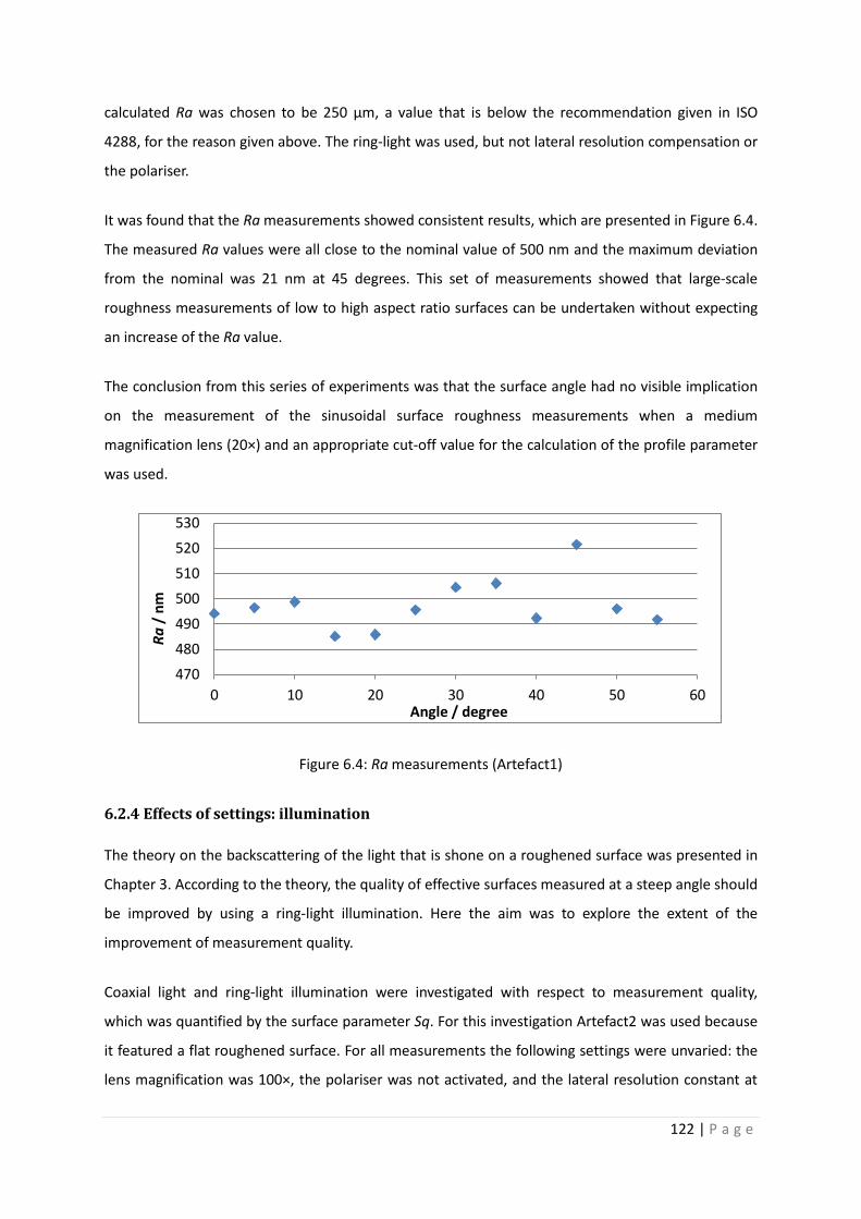
122 | P a g e
calculated Ra was chosen to be 250 μm, a value that is below the recommendation given in ISO
4288, for the reason given above. The ring-light was used, but not lateral resolution compensation or
the polariser.
It was found that the Ra measurements showed consistent results, which are presented in Figure 6.4.
The measured Ra values were all close to the nominal value of 500 nm and the maximum deviation
from the nominal was 21 nm at 45 degrees. This set of measurements showed that large-scale
roughness measurements of low to high aspect ratio surfaces can be undertaken without expecting
an increase of the Ra value.
The conclusion from this series of experiments was that the surface angle had no visible implication
on the measurement of the sinusoidal surface roughness measurements when a medium
magnification lens (20×) and an appropriate cut-off value for the calculation of the profile parameter
was used.
Figure 6.4: Ra measurements (Artefact1)
6.2.4 Effects of settings: illumination
The theory on the backscattering of the light that is shone on a roughened surface was presented in
Chapter 3. According to the theory, the quality of effective surfaces measured at a steep angle should
be improved by using a ring-light illumination. Here the aim was to explore the extent of the
improvement of measurement quality.
Coaxial light and ring-light illumination were investigated with respect to measurement quality,
which was quantified by the surface parameter Sq. For this investigation Artefact2 was used because
it featured a flat roughened surface. For all measurements the following settings were unvaried: the
lens magnification was 100×, the polariser was not activated, and the lateral resolution constant at
470480490500510520530
0 10 20 30 40 50 60
Ra /
nm
Angle / degree

123 | P a g e
1.4 μm. The surface of Artefact2 was measured three times at each angle in the range from 0
degrees to 80 degrees, with 5 degrees increments, once using only the coaxial light (at maximum
intensity) as an illumination source, and the second time using the ring-light and the coaxial light. For
the latter light setting, the ring-light was used at maximum intensity and the coaxial light was used at
10 % to 20 % intensity, in order to equalise the intensities, this being judged subjectively based on
experience. The exposure time (ranging between 4 ms and 8 ms) was adjusted for each surface
angle, not by using a mathematical relation but again by judging the image contrast in the live-view
subjectively.
At each angle the surface was measured three times repetitively. Post-processing of the
measurements involved a least-squares operation, by which each measurement was levelled
horizontally by rotating the surface representation, before calculating the surface parameter Sq for
each image using a cut-off value (λc) of 25 µm.
All obtained Sq values are plotted in Figure 6.5. Very clearly the same trend was apparent in both
sets of measurements taken with different illumination conditions. The measurement results of the
set taken with the additional ring-light is described here and will serve as a comparator to the set of
measurement results obtained from measurements completed with the coaxial light only.
At zero degrees, Artefact2’s surface roughness (Sq) measured with the additional ring-light was
42 nm. At low angles up to 45 degrees the measured Sq value increased gradually at an increment of
approximately 29 nm per 5 degrees. Between 45 degrees and 55 degrees, Sq values increased more
significantly by approximately 144 nm per 5 degrees. The next bracket of surface angles was from
55 degrees to 75 degrees, at which point the Sq value was at a maximum, and the Sq value’s mean
increase was 72 nm per 5 degrees. From 75 degrees to 80 degrees the Sq value decreased by 40 nm.
A FV instrument has specific measuring responses related to surface angle. The results identified four
categories of aspect ratios: low aspect ratio from 0 degrees to 45 degrees, medium aspect ratio from
45 degrees to 55 degrees, high aspect ratio from 55 degrees to 75 degrees and very high aspect ratio
beyond 75 degrees. The upper limit of the angular section ‘medium aspect ratio’ coincided
approximately with the half aperture angle for the 100×, which was 53 degrees.
The set of results from the measurements conducted using the coaxial light source only was very
similar to the Sq-data set for the measurements performed with the additional ring-light
illumination. The major difference between these two sets of measurements was the Sq value for the
measurement at 80 degrees with coaxial illumination only. This outstanding value, however, was

124 | P a g e
treated as an outlier for the reason that no subsequent set of results feature this particular
measurement behaviour. The measurement was singular, so no repeatability value could be attached
to the measured result. Minor differences in Sq of both sets of measurements lie within the low
aspect ratio region, in which the coaxially illuminated measurements showed larger Sq values by
15 nm consistently, and in the high aspect ratio region, where the Sq values measured with only
coaxial illumination were consistently lower than the related set of measurements by 70 nm. The
standard deviations were smaller for the measurements with the ring-light illumination, but in
general relatively small compared to the measured Sq values (the largest being 93 nm and 43 nm
respectively for the coaxial and the ring-light illumination set of measurements).
Figure 6.5: Influence of coaxial and ring-light with coaxial illuminations (Artefact2)
6.2.5 Effects of settings: polariser
The influence of the polarising filter was investigated for measurements of the roughened surface at
different aspect ratios using the 100× objective lens. The effect was expected to be positive (i.e. to
lower Sq) because the polariser diminishes the amount of specular reflection captured by the
camera, thus lowering the amount of spikes in the effective surface. The settings were as described
previously: the lateral resolution was kept constant at 1.4 µm, ring-light illumination at 100 %, and
coaxial light illumination at approximately 15 %. The differences were the added polariser within the
optical path, and the exposure times, which were adjusted for each individual measurement.
Artefact2 was measured with the polariser from 0 degrees to 80 degrees in 10 degree increments
because it was found from the previous sets of measurements that 10 degree increments was
0
0.5
1
1.5
2
2.5
0 10 20 30 40 50 60 70 80
Sq /
µm
Angle / degrees
coaxial ring

125 | P a g e
sufficient to show the performance characteristics. At each angle three measurements were
completed repeatedly. Post-processing of the measurements followed the same process as defined
for previous measurements. The 3D imaged surfaces were levelled and the Sq parameter was
calculated using a cut-off value (λc) of 25 μm.
Figure 6.6 shows the two sets of measurement results, which resembled each other in their general
trends, as seen in the previous experiment. For the measurements with the polarisation, the Sq
values increased by approximately 27 nm per 5 degrees on average in the low aspect ratio region.
When the surface angle neared the half aperture angle, the Sq values stepped up by approximately
77 nm per 5 degrees and beyond the half aperture limit Sq increased only by 48 nm per 5 degrees.
The maximum Sq value was measured at 70 degrees, and at 80 degrees a smaller Sq was measured.
In comparison to the comparable set of measurements completed without the polariser (Figure 6.6),
the Sq values only differed significantly for medium and high aspect ratio measurements (i.e. from
50 degrees onwards). Above 50 degrees the increase in Sq for the measurements with polarisation
was more gradual, and the maximum Sq value was 70 % (257 nm difference) of the maximum Sq
value when measuring the surface without the polarisation. The largest standard deviation of the set
of measurements with the polariser was 46 nm, which was comparable to the largest standard
deviation of the other set of measurements (43 nm).
Figure 6.6: Influence of the polariser (Artefact2)
0
0.2
0.4
0.6
0.8
1
0 10 20 30 40 50 60 70 80
Sq /
µm
Angle / degrees
ring ring+pol

126 | P a g e
6.2.6 Effects of settings: lateral resolution compensation
The sampling distance is a constant specific for each objective lens. From all the points recorded,
which are separated by the sampling distance, the focused areas are calculated and thus the lateral
resolution is larger than the sampling distance. Since the lateral resolution is a result of data
processing, it can be a variable, and on the IFM G4 system the lateral resolution can be set with a
slide bar. This approach is good only if the surface is level. However, in the case that the object’s
surface is sloped, the target resolution is not obtained due to the aspect ratio. In order to achieve
the target lateral resolution of the surface (LR0), the imaging lateral resolution (LRφ) can be changed
to a value that takes the surface angle (φ) into account according to Equation 6.2 below.
𝐿𝑅𝜙 = 𝐿𝑅0 × cos𝜙 6.2
The last set of measurements presented here was designed to be compared to the set of
measurements that was obtained with coaxial light illumination only, for which the constant lateral
resolution was 1.4 µm. Therefore, neither the polarised filter nor the ring-light illumination were
used for the measurements; the exposure times were similar to the set of measurements used for
the comparison (Table 6.2). The surface roughness was measured at 10 degree increments from
0 degrees to 80 degrees. The only difference in settings was the addition of lateral resolution
compensation linked with the angle of inclination of the surface according to Equation 6.2.
Table 6.2: Lateral resolutions (LR) for the compensation of the surface aspect ratio
Angle
(degrees)
LR
(nm)
Angle
(degrees)
LR
(nm)
0 2600 40 1991
5 2590 45 1838
10 2560 50 1671
15 2511 55 1491
20 2443 60 1300
25 2356 65 1098
30 2255 70 889
35 2129 75 672
80 451

127 | P a g e
At 0 degrees the nominal Sq value for Artefact2’s surface (21 nm) was less than half the value of the
comparator data Sq (55 nm) obtained with a lateral resolution of 2600 nm. For the set of
measurement results, Sq, showed a gradual increase with respect to the surface angle in the range
from 0 degrees to 40 degrees, similar to the observations in the previously presented sets of
measurements. Here, the gradual increase was approximately 33 nm per 5 degrees on average. The
measured surface roughness doubled from the measurement at 40 degrees to the measurement at
50 degrees, from 287 nm to 552 nm. Above 50 degrees Sq increased minimally (7 nm per 5 degrees).
At 70 degrees the maximum surface roughness Sq was registered and at 80 degrees, the measured
surface roughness decreased slightly, by 57 nm. The results are shown in Figure 6.7. The standard
deviation of the measurements with lateral resolution compensation was in general smaller, the
maximum value being 33 nm, compared to 96 nm.
Overall results indicated an improvement of the quality of the effective surface. The improvement
was up to 30 % for measurements of high aspect ratio surfaces when the surface angle was
compensated for by reducing the lateral resolution. For surface angles below 40 degrees, the
measurement results suggest that the lateral resolution compensation was not necessary.
Figure 6.7: Influence of lateral resolution compensation coupled to the surface angle (Artefact2)
6.2.7 The effect of different surface roughness
FV relies on surface roughness to give contrast in the focused areas in each measurement frame. A
comparison between the measurements of two artefacts roughened with the same method but two
different levels of roughness (Artefact2 and Artefact3) should provide experimental evidence for
surfaces with a larger roughness are better measured at high surface angles using the FV technique.
Both artefacts were measured from 0 degrees to 80 degrees in 10 degree increments and three
0
0.5
1
1.5
2
2.5
0 10 20 30 40 50 60 70 80
Sq /
µm
Angle / degrees
coaxial coaxial+lat

128 | P a g e
times repeatedly at each angle. For both sets of measurements, the polariser was not used; the ring-
light was not used; and the lateral resolution was compensated for the respective angles, using a
lateral resolution of 2600 nm for the surface measurement at 0 degrees and the subsequent lateral
resolutions were calculated with Equation 6.2. For the calculation of Sq, each of the surface images
were levelled (using the software provided by Alicona) and the parameter calculated with λc = 25 µm.
The trends of both sets of measurement results (displayed in Figure 6.8) showed a strong similarity
to previous measurement results, with elements of interest. Horizontal measurements with these
specific settings indicated that Artefact2 had a Sq value of 66 nm, and that Artefact3’s surface
roughness Sq was 145 nm (over double the roughness of Artefact2).
The measurement results of Artefact2 showed a gradual increase of Sq in relation to the surface
angle (33 nm per 5 degrees) up to 40 degrees. At 40 degrees, the difference in the measured Sq
value was approximately threefold of the previous mean increase (107 nm per 5 degrees). The
maximum surface roughness was measured at 60 degrees, whilst in previous measurement results
the maximum was found at 70 degrees. Here, Sq at 70 degrees was lower than the measurement at
80 degrees, which was another feature not present in previous sets of measurement results and
seems to be an inexplicable outlier.
The minimum Sq value of the measurements of Artefact3 was measured at 10 degrees (118 nm), a
trend characteristic that was not found in previous sets of results. From 10 degrees onwards, the Sq
value rose similarly to the measurement results of Artefact2. The difference in Sq between the
surfaces measured at 40 degrees and 50 degrees (114 nm) were not outstandingly larger than the Sq
difference at 30 degrees to 40 degrees (122 nm). At angles above 50 degrees, the trend of the
measured Sq values had a smaller differential. The standard deviations for both sets of
measurements were relatively small, with the exception for the measurement of Artefact2 at
60 degrees, for which the standard deviation was 60 nm.

129 | P a g e
Figure 6.8: Measurements of two differently rough surfaces (Artefact2 and Artefact3)
6.2.8 The effect of profile length on Ra and of λc on Sq
This examination of one particular data set had the aim to demonstrate how the calculation of Ra
depends on the length of the profile used for the calculation, and how λc may influence the quality of
Sq. To investigate this issue, the data presented in Section 6.2.4 was reprocessed. Artefact2 was
measured three times repetitively at angles from 0 degrees to 80 degrees with 5 degree increments
using ring-light illumination and the 100× objective lens, and a specific compensated lateral
resolution for every surface angle according to Table 6.2.
Four sets of surface texture parameters were calculated, of which the first two, and the latter two
sets are comparable: Ra was averaged over five line profiles (Ra_5, total profile length: 740 µm), Ra
was averaged over 500 line profiles (Ra_500, total profile length: 74 mm) using λc = 80 µm for the
calculation of Ra, and two Sq values, one calculated with λc = 80 µm and the other with λc = 25 µm.
Theoretically, the rotational orientation of the random inhomogeneous surface (Artefact2) within the
angled plane should have no implication on the roughness parameter Ra.
6.2.8.1 Ra-parameters
The numerical results of Ra_500 values plotted in Figure 6.9 showed a clearer trend than the results
from Ra_5 values, which had a larger dispersion. Therefore, the Ra_500 results will be discussed first
and used as a comparator for Ra_5 results. The Ra values of Artefact2 measured at 0 degrees was
5 nm. This parameter’s value increased steadily up to 77 nm at 35 degrees (10 nm per 5 degrees), at
40 degrees a Ra value of only 48 nm was measured and for the following two measurements at
45 and 50 degrees the measured Ra value increased to 95 nm, increasing by 23 nm per 5 degrees.
The surface measurement at 55 degrees gave back a smaller Ra (83 nm) and the subsequent two Ra
00.10.20.30.40.50.60.70.8
0 10 20 30 40 50 60 70 80
Sq /
μm
Angle / degrees
Artefact2Artefact3
130 | P a g e
measurement results at higher angles increased. The maximum Ra value was measured when the
surface was inclined at 65 degrees. Measurements of surfaces tilted beyond 65 degrees showed
decreasing Ra values. At 80 degrees the test surface was measured to have a Ra of 39 nm, which is in
the range of the Ra value measured at 20 degrees.
If the surface inclinations had been classified in low, medium, high and very high aspect ratio based
on these results, then each class would have agreed approximately with the classification given in
Section 6.2.4: low aspect ratio ranges from 0 degrees to 40 degrees, 40 degrees to 55 degrees
formed the band of medium ratio angles, followed by the high ratio angles from 55 degrees to
70 degrees and the last band was the very high aspect ratio band that included all angles beyond
65 degrees.
These aspect ratio bands defined above were also reflected in the results of the Ra measurements
using only 5 lines for the parameter calculation. The only discrepancy between these two sets of
measurements was the upper limit of the medium aspect ratio band, which for the Ra_5
measurements lay at 55 degrees.
In general, it was noticeable that the Ra_5 values were considerably larger. The reason for the larger
Ra_5 values was because the Ra calculation of a longer profile mitigates the influence of noise. In the
low aspect ratio band the maximum Ra_5, recorded at 35 degrees, was 211 nm, almost three times
the equivalent Ra_500 value (274 %). The maximum Ra_5 in the medium aspect ratio band was 250
nm, 263 % greater than the Ra_500 value at 50 degrees. The largest Ra_5 was measured at 65
degrees, 289 nm, which differs from the Ra_500 value by 178 nm. At the highest angle measured (80
degrees) the calculated parameter was 134 nm and comparable to the measured Ra_5 at 30 degrees.
Both sets of results showed trends which were comparable to each other; however, they were not
comparable to areal parameters (i.e. Sq). Despite the different overall trends between the results of
areal and profile parameters, it was possible with both types of parameters to classify the angles of
surface inclination in four aspect ratio groups, with very similar angular boundaries. Both sets of
measurements had significant standard deviation values, the largest of which were attached to the
measurements measured at 80 degrees, 43 nm and 36 nm respectively for the sets of measurements
using 5 lines and 500 lines for the averaging. This standard deviation ratio (1.2 : 1) was approximately
constant for all other measurement pairs.

131 | P a g e
Figure 6.9: Effect of averaging Ra-values over 5 and 500 line measurements (Artefact2)
6.2.8.2 Sq-parameters
The seventeen surface measurements used for the investigation of Ra calculations were also used to
investigate the effect of cut-off values (λc), on Sq. The two chosen λc parameters were 25 μm and
80 μm, and the associated Sq parameters were abbreviated with Sq_25 and Sq_80. The cut-off value
80 μm was chosen for the reasons given above, and the second cut-off value was chosen to be
further from the recommended value (250 μm) so that the performance characteristics would be
more pronounced.
The overall shape of both sets of measurement results (shown in Figure 6.10) was the same as seen
in Section 6.2.4. An observation was that all Sq_80 values with respect to their angular equivalent
Sq_25 values were consistently larger. At increasing surface angles the difference between Sq_80 and
Sq_25 increased gradually: at 15 degrees the difference was 17 nm, 22 nm at 30 degrees, 36 nm at
45 degrees, 32 nm at 60 degrees, and 49 nm at 75 degrees. Overall, the different cut-off values used
for the evaluations of the surfaces only made small numerical differences. The standard deviations
were insignificant, the largest being 42 nm for both sets of measurements at 80 degrees.
0
0.05
0.1
0.15
0.2
0.25
0.3
0.35
0 10 20 30 40 50 60 70 80
Ra /
µm
Angle / degrees
Ra_5Ra_500

132 | P a g e
Figure 6.10: Effect of λc for calculating Sq (λc = 80 μm and λc = 25 μm) (Artefact2)
6.2.9 Comparison between the IFM G4 and the PGI
Stylus instruments are commonly regarded as the most accurate of surface topography instruments.
This conception exists because the mechanical interaction of stylus tips with the surface is
understood intuitively: the movement of the tip tracing the surface can be imagined visually.
Additionally, the sources of error are better understood, such as mechanical filtering due to the
probe tip curvature (Petzing et al., 2010). Light ray tracing, in comparison, is more difficult to
comprehend. However, both areal and profile techniques, have their advantages and disadvantages
and this section aims to show the differences of profile measurements between both techniques,
when angling the surfaces up to 40 degrees.
Presented here are surface profile measurements of low aspect ratio surfaces (up to 40 degrees)
using the IFM G4 and a stylus instrument (PGI 1250 by Taylor Hobson). Measurements with the IFM
G4 were carried out without the ring-light or the polariser, with the 100× objective lens, and with a
lateral and vertical resolution of 1.4 µm and 20 nm, respectively. The specifications of the PGI as
used for the measurements were a lateral resolution of 16 nm, a vertical resolution of 0.8 nm, a
stylus length of 60 mm, a conical tip with a radius of 2 μm. The calibration certificate (dated June
2013) of the PGI used here specified an error of 3 nm when measuring a 300 nm roughness artefact.
The measurement procedures were designed so that the results of measurements with both
instruments were comparable. Artefact3 was measured three times repeatedly at angles ranging
from 0 degrees to 40 degrees with 10 degree increments, thus obtaining thirty profiles in total. All
profiles were then levelled rotationally and characterised by their Ra parameter value, which was
0
0.2
0.4
0.6
0.8
1
1.2
1.4
1.6
0 10 20 30 40 50 60 70 80
Sq /
µm
Angle / degrees
Sq_80Sq_25

133 | P a g e
calculated with a cut-off value of 80 μm. In order to avoid discrepancies due to different surface
texture software, the Mountains software V5 was used for the evaluation of all measurements.
The Ra values measured by both instruments are plotted against the surface angle (Figure 6.11). A
common feature between both sets of measurements was the quadratic behaviour at high angles;
however, the derivative of the trend of the PGI results was negative, whilst the roughness measured
with the IFM G4 increased with respect to surface angle. The two averaged roughness values
measured at 0 degrees disagree with 17 nm difference. At 20 degrees, there is a negligible numerical
difference in measured roughness by both techniques. The Ra measurement of the PGI at 0 degrees,
10 degrees and 20 degrees varied only by 0.2 nm in comparison to the equivalent of 17 nm for the
measurements with the IFM G4. At 30 degrees and above, the difference in Ra is 23 nm at 30
degrees and 88 nm at 40 degrees.
Figure 6.11: Measurement of Ra using the IFM G4 and the PGI (Artefact3)
6.3 Discussion and conclusions
The work reported here presents experimental evidence for the effect of different combinations of
settings on low to high aspect ratio measurements performed with a FV technique. On a
fundamental level, the measurement of very high aspect ratio surfaces (up to 80 degrees)
demonstrated that the FV technique was capable of constructing an effective surface with few
defects such as spikes or holes.
In each of the experiments the measurement quality was assessed in terms of a profile or surface
parameter. For measurements carried out with the IFM G4, the parameter value would generally
increase when measuring a specific artefact at different angles. With regard to this trend, a change
0
20
40
60
80
100
120
0 5 10 15 20 25 30 35 40 45
Ra/
nm
Angle/ degrees
IFM G4 PGI
134 | P a g e
of experimental set up (artefact or setting) that consistently lowers the trend numerically (especially
for aspect ratio measurements beyond the numerical aperture) was considered a positive influence
on the measurement because that brought the parameter closer to the parameter value measured
at 0 degrees.
Against expectations, the addition of ring-light as a source of illumination did not significantly
improve the image quality in terms of Sq. A reason for this outcome may have been human error:
the light sources may not have been balanced appropriately. However, it should be emphasized that
this set of measurements was carried out after a year of experience with the instrument (including a
training course) thus putting the weight of human error in question. Another reason could be the
presence of only one surface gradient, which facilitated the adjustment of exposure time.
Consequently, the ring-light had not significant improvement on the high aspect ratio surface
measurements.
Comparative measurements with the polariser showed that a negligible difference was detected at
angles lower than 50 degrees. The half aperture angle for the 100× lens used was 53 degrees, so a
significant difference in using the polariser started to show just before the half aperture angle was
reached. The results indicate that for angled surface measurements, the polariser was necessary for
surface angles just below the lens' half aperture angle and beyond, improving the measurement
results up to 30 %. It should be noted that this set of measurement results was specific to the
material (stainless steel) and the surface finish (roughened by method of particle blasting).
The lateral resolution compensation had a similar effect on the measurement results as the
polariser: the results showed that lateral resolution compensation was only effective when the
surface angle was just below the lens' half aperture angle and up to very high aspect ratio surfaces.
Improvements were also as much as 30 %. A practical problem with the lateral resolution
compensation occurs when the measurand is not planar and different surface angles are present in
one image field. For such cases, the highest necessary lateral resolution could be used as a setting,
but this would come at the cost of measurement time. In any case, local Sq values will differ over a
measured surface with a non-planar form.
Surface roughness on the nano-scale was a very important detail of surface measurements when
using a FV instrument. A comparison of two sets of measurements taken of two differently rough
surfaces at a range of angles showed better results for the rougher surface (up to 27 %), which
above the lens' numerical aperture showed a clear trend. On the contrary, measurements of the
smoother surface showed more fluctuation.
135 | P a g e
The comparative study concerning parameters showed that beyond 10 degrees it was increasingly
important to have a very long profile, from which the Ra parameter was calculated. This was due to
the higher level of noise or re-entrant features (spikes, etc.). The Ra value calculated from a length
one hundred times longer than a second length could improve the result by up to 62 %. Areal
surface texture measuring instruments have the advantage of measuring multiple profiles after only
one measurement (of a surface area); an ability that should be exploited especially when measuring
high aspect ratio surfaces.
The effect of using a smaller cut-off value showed a constant but small difference of approximately
5 %. This result showed that choosing a cut-off value without following the suggestion given in
ISO 4288 does not necessarily have a major impact on measurements of angles surfaces.
The measurements with the PGI and the IFM G4 showed contrasting trends: the PGI measured
smaller Ra values at higher angles and the IFM G4 measured larger Ra values at higher angles,
resulting in a difference of 123 % at 40 degrees. Although the PGI can measure surfaces up to
40 degrees with a comparatively small Ra deviation, the IFM G4 can measure beyond 40 degrees,
however, with a poorer Ra result. This set of measurements emphasized the importance to know
the instrument behaviour when performing measurements without ideal measuring conditions. The
results also showed that the stylus and the optical measurements at 0 degrees do not agree. The
fact that the PGI gave roughness measurement results that only deviated by 5 % on angles up to
20 degrees reinforces the common thought that stylus instruments may provide surface texture
measurements with more confidence.
In summary, the conclusions were as follows:
• The ring-light illumination method improved the high aspect ratio measurements (above the
half aperture) angle by approximately 5 %.
• The polariser improved the high aspect ratio measurements by approximately 30 %.
• The lateral resolution compensation improved the high aspect ratio measurements by
approximately 30 %.
• A larger roughness improved high aspect ratio measurements in terms of standard
deviation.
• A larger number of Ra values used for averaging is important for high aspect ratio
measurements (improvement of 60 %).
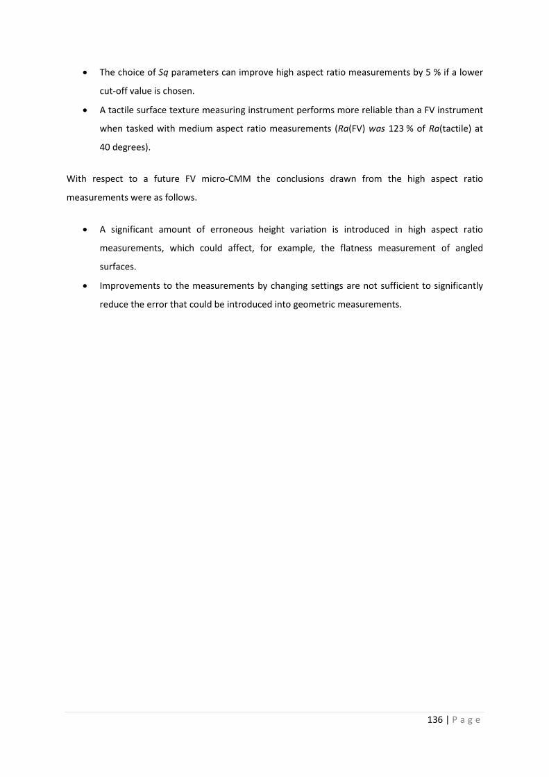
136 | P a g e
• The choice of Sq parameters can improve high aspect ratio measurements by 5 % if a lower
cut-off value is chosen.
• A tactile surface texture measuring instrument performs more reliable than a FV instrument
when tasked with medium aspect ratio measurements (Ra(FV) was 123 % of Ra(tactile) at
40 degrees).
With respect to a future FV micro-CMM the conclusions drawn from the high aspect ratio
measurements were as follows.
• A significant amount of erroneous height variation is introduced in high aspect ratio
measurements, which could affect, for example, the flatness measurement of angled
surfaces.
• Improvements to the measurements by changing settings are not sufficient to significantly
reduce the error that could be introduced into geometric measurements.

137 | P a g e
Chapter 7: Geometric measurements using FV
7.1 Introduction
This chapter presents geometric measurements completed with the IFM G4 with the intention to
investigate how well the FV technique can measure simple geometric features. These sets of
measurements were conducted with the view to investigating suitable measurement procedures
and a potential re-verification artefact for the assessment of instrument performance, when the FV
technique has been implemented as a micro-CMM system. The results obtained from these
geometric measurements are part of the foundation for Chapters 8 and 9.
Originally the IFM G4 was only intended for surface topography and form measurements; therefore,
the instrument possesses software functions (V3.5) that allow limited geometric measurements. The
simple geometric features inspected here were a roughened flat (Artefact2, previously used in
Chapter 6), gauge blocks and spheres. It was necessary to be aware of external influences on the
error of the measured geometrical feature. Such influences would be associated with the
measurement set-up or the artefact used.
7.2 Geometric angle measurements
7.2.1 Introduction
In the context of micro-CMMs is it important that the FV technique’s geometric measurements are
not affected by the quality of the effective surface, i.e. data holes and spikes. The advantage that
areal instruments have over touch probes is that they can measure a significantly larger amount of
data per unit area that can be used for fitting geometric shapes.
The purpose of measuring the angle of a surface with respect to the horizontal XY plane of the
instrument’s co-ordinate system was to investigate if a relationship existed between the quality of
the surface and the spread of results (variation, in terms of one standard deviation) of geometric
angle measurement. Chapter 6 identified a relationship between the angle of the surface and the Sq
parameter, therefore, it could be expected that the results of the plane fitting procedure (using a
Gaussian best-fit method) were more spread out for surfaces measurements with high aspect ratio.
This assessment should give information on the capability of the FV technique to measure angles.
The standard deviation of the measurement results embodies the measurement uncertainty to
measure geometric angles, which are influenced by dust particles and the specimen’s form deviation.

138 | P a g e
7.2.2 Assessing the variation of angle measurements
A set of data sets were taken from the high aspect ratio surface texture measurements (Chapter 6)
and re-used for the assessment of standard deviation of angle measurements. This data set
comprised of three measurements at each angle and the angles ranged from 0 degrees to
80 degrees with 5 degrees increments, so three measurements were completed at all 17 angles,
amounting to 51 measurements in total. The measurements of the same surface angle were
repeated successively so that the measurement set-up would not influence the standard deviation
of angle measurements.
The measurement procedure to obtain the effective surfaces has already been stated in Chapter 6:
angle gauges were used to realise the nominal angle of a roughened surface (Artefact2). No soft
materials were used to position the roughened surface, to ensure that the surface would not
displace during the time of measurement (approximately 2 minutes). The 100× magnification lens
was chosen because of its large numerical aperture but the drawback to this choice is the small field
of view. The measurement settings were as shown in Table 7.1:
Table 7.1: Settings for the angle measurements
Type of setting Setting for angle measurements
Lens magnification 100×
Coaxial light 10 % - 20 % of maximum intensity
Ring-light 100 % of maximum intensity
Exposure time 4 ms – 8 ms
Contrast Constant at 0.9
Lateral resolution Constant at 1.20 μm
Vertical resolution Constant at 46 nm
Polariser Not applied
7.2.3 Results
The results are shown in two graphs: the first graph (Figure 7.1) displays the angle measurement
deviation from the nominal with one standard deviations error bars (± 1 σ) and the second graph
(Figure 7.2) presents the standard deviations for the measurements at each angle. In the context of
assessing the instrument capability, the second graph is of more importance because the standard
deviation is not affected by measurement set-up errors such as improper wringing of gauge blocks.

139 | P a g e
The first graph shows that the angle measurements were recorded within a band of ± 0.2 degrees
from the nominal value, with the exception at 50 degrees where the measurement deviation was
0.45 degrees. This indicated that the measurement behaviour at approximately the half aperture
angle differed from the measurement behaviour at other angles.
The absolute mean angle deviation was smallest at 0 degrees (0.02 degrees) and gradually increased
for the angles up to 20 degrees (0.16 degrees) and the spread of measurements also increased
although small (standard deviation was up to 0.07 degrees). The absolute deviations of the angles
measured between 25 degrees and 40 degrees were small (up to 0.07 degrees), however, their
associated standard deviations were larger than before (up to 0.25 degrees). For the measurement
of angles 45 degrees to 55 degrees, the absolute mean deviations were large and the set included
the outlier (0.2 degrees, 0.45 degrees and 0.2 degrees) and their spread of measurements were the
largest of all measured angles (0.35 degrees). Measurements of the roughened surface at 60 degree
to 80 degrees did not show any significant characteristic. Their mean measurement deviations were
scattered within the ± 0.17 degrees band from the nominal angle value and their standard deviations
did not exceed 0.21 degrees.
The graph that displays the standard deviations for each angle (Figure 7.2) shows an approximately
increasing trend up to the measurements at 55 degrees. This angle coincides approximately with the
half aperture angle of the 100× lens that was used for all measurements. At angles beyond
55 degrees, the standard deviations were lower. This indicates that the effective surfaces measured
up to 55 degrees were of increasingly poorer quality (also in accordance with the texture
measurements (Sq) in Chapter 6). The introduction of spikes and holes to higher aspect ratio
surfaces measurements influenced the plane fitting procedure. The plane fitting method was less
affected by the poorer quality of the effective surfaces measured beyond 55 degrees. This is an
indication that the cause for the degradation of measurement quality at high aspect ratio
measurements is of a different nature than that of lower aspect ratio measurements: the first may
be predominantly re-entrant features, and the latter is more likely to be spikes.

140 | P a g e
Figure 7.1: Mean deviation of the measured angle from the nominal value (± 1 σ)
Figure 7.2: 1 σ of measurements at each angle
7.2.4 Conclusions
As identified in the introduction (Section 7.2) the purpose of the angle measurements was to explore
the variation of angle measurements in order to assess the suitability of the FV technique for angle
measurements. Evidence from Chapter 6 showed that the quality of the effective surface was
related to the angle of the surface at which it was measured, such that the quality became poorer
with increasing surface angle. Reasons for the decrease in quality were the presence of spikes, holes
and re-entrant features, due to the decreased amount of information gathered from the surface.
These features were expected to affect the angle measurement of the surface.
The variation of angle measurements was successfully assessed by fitting planes to 51
measurements of angled surfaces (17 angles, 3 repeats) using one set of settings for all
measurements. The variation assessment (in terms of 1 σ) indicated a predictable relationship
between the measurement variation and the surface angle up to the half aperture angle: the
-0.4
-0.2
0.0
0.2
0.4
0.6
0.8
1.0
0 10 20 30 40 50 60 70 80
Angl
e de
viat
ion
/ d
egre
es
Nominal angle / degrees
0.0
0.1
0.2
0.3
0.4
0 10 20 30 40 50 60 70 80
Stan
dard
dev
iatio
n /
degr
ees
Nominal angle / degrees

141 | P a g e
variation increased with increasing surface angle at an approximate ratio of 1:15. Beyond the lens’
half aperture angle the variation showed the same trend as before, but only after the variation
dropped off significantly at 60 degrees (down to 0.06 degrees).
In the context of FV micro-CMM, this work highlighted the need to decrease the variation of plane-
fitting procedures, aside from measurement set-up related errors, such as dust or improper wringing
of gauge blocks or the specimen’s form error, in order to improve measurements of angled flat
(roughened) surfaces. With respect to the development of a re-verification artefact for a FV micro-
CMM, this work also provided significant information: the variation of a shape-fitting procedure to a
high aspect ratio surface measurement is larger than the variation of a shape-fitting procedure to a
low aspect ratio surface measurement. Therefore, the re-verification artefact should ideally not
feature high aspect ratio surfaces that are crucial to dimensional measurements with the objective
to improve the measurement performance of the re-verification artefact.
7.3 Length measurement error assessment using gauge blocks
7.3.1 Introduction
The aim of measuring the lengths of gauge blocks was to investigate the applicability of the FV
technique to length measurements of prismatic shapes. The reason for conducting this assessment
was the suggestion in ISO 10360 to use, amongst others, prismatic shapes, such as gauge blocks or
step gauges, for the length measurement error assessment of CMMs and it was necessary to
establish if this held true for the FV technique. The information gained from this set of measurement
should also provide guidance on a possible development of a re-verification artefact for FV micro-
CMMs.
7.3.2 Methods for gauge block measurements
As for the previous experiments, the length measurements of gauge blocks were completed using
the IFM G4 in the same stable environmental conditions, with a temperature of 20 °C ± 0.5 °C and a
humidity of 50 % ± 10 % rH.
The lengths were defined by a range of five differently sized Mitutoyo stainless steel gauge blocks
(grade 1) with nominal lengths of 1.0 mm, 3.0 mm, 4.0 mm, 8.0 mm, and 16.0 mm, for which the
specifications are given in Table 7.2. The lengths were chosen because each of the gauge blocks, in
the above sequence, had to be measured with an increasing number of FoVs to complete a line scan.
The total length of all gauge blocks (32.0 mm) was approximately one half of the length

142 | P a g e
recommended by ISO 10360 (66 % of total displacement in a given measurement orientation) to re-
verify the X and Y orientations of a cubic measurement volume defined by a 100 mm edge length. It
was expected that half of the recommended length was sufficient to provide evidence on the
performance of FV instrument when tasked to measure the length of a prismatic object along the X
and Y orientations.
Table 7.2: Specifications of Mitutoyo stainless steel gauge blocks (grade 1)
Nominal
length
(mm)
Central
deviation
(μm)
Maximum
deviation
(μm)
Minimum
deviation
(μm)
Variation
(μm)
Code
number
1.0 +0.03 +0.04 +0.02 0.02 611611
3.0 +0.05 +0.05 0.00 0.05 611613
4.0 +0.03 +0.03 -0.03 0.06 611614
8.0 +0.04 +0.06 +0.02 0.04 611618
16.0 +0.10 +0.11 +0.06 0.05 611626
For all measurements, the gauge blocks were arranged in the same sequence as listed above, such
that their wringing surfaces were in contact, using three different configurations that are explained
below. The measurement orientations were in parallel to the X and Y axes of the IFM G4’s XY stage.
Two additional gauge blocks were positioned on both sides of the assembled set of five gauge blocks,
in order to bracket these, so that the definition of the lengths are identical for all.
Off-the-shelf gauge blocks have chamfers around the wringing surface, as was the case for those
used for these experiments. The problem with the chamfers is that they introduce tilted surfaces of
varying angles into a line scan measurement (shown in Figure 7.3), forming V-grooves that are
difficult to measure because of non-ideal lighting conditions. The grooves would be underexposed
and the flat surfaces overexposed causing an elevated level of measurement noise (approximately
190 %, see Chapter 4). The low-quality measurements of the underexposed V-grooves would affect
the accuracy of locating borders between two gauge blocks, which has a direct consequence on the
accuracy of distance measurements. Therefore, the chamfers of all gauge blocks were removed by
grinding off a layer of a non-wringing surface, such that the calibrated lengths are minimally affected
by the grinding process. A recalibration of the gauge blocks was not performed because the
measurements of the gauge blocks with the IFM G4 produces very large uncertainties as shown in

143 | P a g e
the following. In addition the machining of the gauge blocks would have produced a systematic error,
which was also not visible in the results.
Figure 7.3: Effect of chamfers on the profile of wrung gauge blocks
7.3.2.1 Configuration 1: wrung gauge blocks
In the first configuration for length measurements using gauge blocks, they were wrung together and
placed in a gauge block clamp. A linear measurement was run over all five gauge blocks on the
surface between two wringing surfaces (as indicated by the white line in Figure 7.4) and partly over
the two bracketing gauge blocks, using the 2.5×, 5×, 10×, 20× and 50× magnification lenses provided
with the IFM G4. Note that the gauge block clamp and one of the bracketing gauge blocks are not
shown) A linear measurement is in this context an image field with only one row or one column
when measuring in the X and Y orientations, respectively, with the overlapping areas being 10 % of
the FoV on each side. The settings used for all measurements are given in Table 7.3. The set-up of the
gauge blocks was not altered for the duration of all repeated measurements to avoid errors caused
by assembling and disassembling of the wrung gauge blocks. The gauge blocks were measured in the
X and Y orientations of the XY stage.
Figure 7.4: Assembled gauge blocks with an indication of the scan (white line)
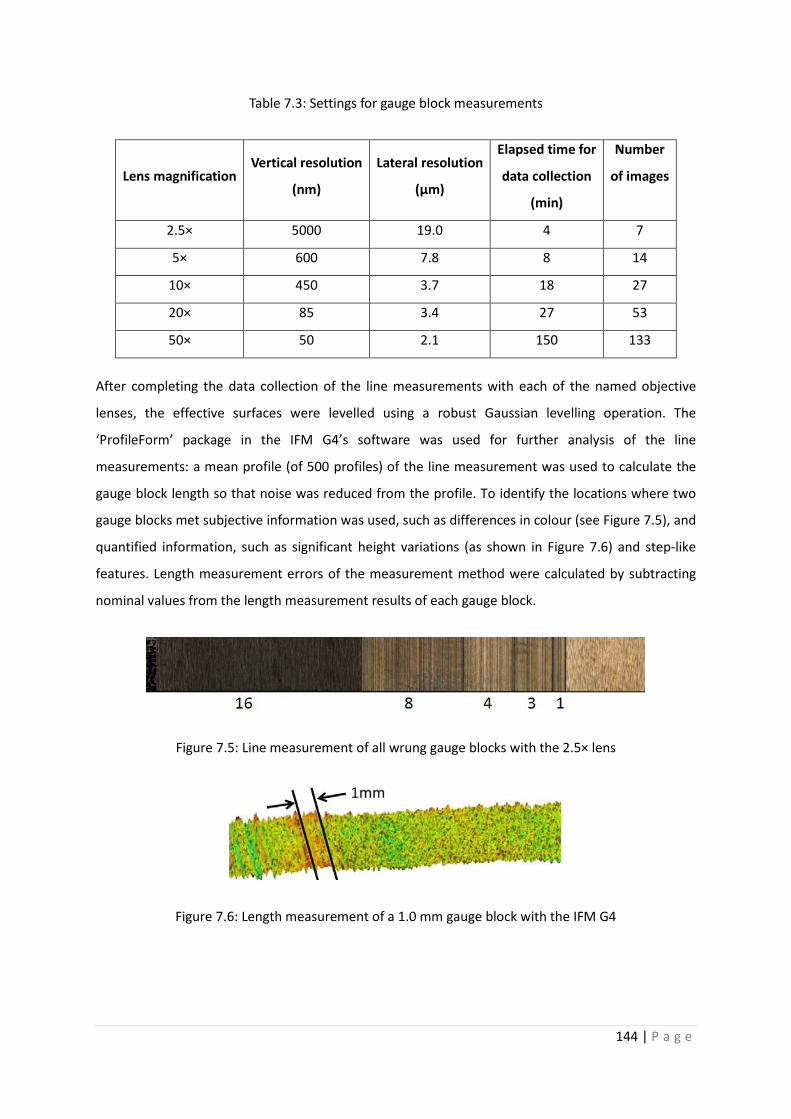
144 | P a g e
Table 7.3: Settings for gauge block measurements
Lens magnification Vertical resolution
(nm)
Lateral resolution
(μm)
Elapsed time for
data collection
(min)
Number
of images
2.5× 5000 19.0 4 7
5× 600 7.8 8 14
10× 450 3.7 18 27
20× 85 3.4 27 53
50× 50 2.1 150 133
After completing the data collection of the line measurements with each of the named objective
lenses, the effective surfaces were levelled using a robust Gaussian levelling operation. The
‘ProfileForm’ package in the IFM G4’s software was used for further analysis of the line
measurements: a mean profile (of 500 profiles) of the line measurement was used to calculate the
gauge block length so that noise was reduced from the profile. To identify the locations where two
gauge blocks met subjective information was used, such as differences in colour (see Figure 7.5), and
quantified information, such as significant height variations (as shown in Figure 7.6) and step-like
features. Length measurement errors of the measurement method were calculated by subtracting
nominal values from the length measurement results of each gauge block.
Figure 7.5: Line measurement of all wrung gauge blocks with the 2.5× lens
Figure 7.6: Length measurement of a 1.0 mm gauge block with the IFM G4

145 | P a g e
7.3.2.2 Configuration 2: staggered gauge blocks
The second configuration of gauge blocks was to stagger non-wrung gauge blocks as shown in Figure
7.7. The primary reason for testing this configuration was to avoid the method of using subjective
information to locate the borders between gauge blocks (as was necessary for the first
configuration). The secondary reason for this configuration was to investigate if the accuracy of edge
definition affected the dimensional measurement.
For the measurements, the gauge block holder as depicted in Figure 7.7 was laid onto its side so that
the line measurements could be set up in order to measure a gap for the gauge blocks that were set
back in the gauge block holder. An example of a line measurement is shown in Figure 7.8. For all line
measurements the same settings as stated in Table 7.3 were used. The results of length
measurement errors were obtained by following the same procedure as with the first gauge block
configuration. The estimated variation of the separation between the gauge blocks was < 1 μm.
Figure 7.7: Staggered gauge blocks
Figure 7.8: Line measurement of all staggered gauge blocks with the 2.5× lens
7.3.2.3 Configuration 3: non-wrung gauge blocks
The third configuration of the gauge blocks was similar to the first configuration with the difference
that the gauge blocks were not wrung together and the line-scans were run over the side of all gauge
blocks. The reason for performing this set of measurements was to investigate the effect of wringing
gauge blocks on the length measurements using the FV technique. A line measurement was
performed over all gauge blocks using the same measurement procedure and settings as described
for the first configuration of gauge blocks.

146 | P a g e
7.3.3 Results
7.3.3.1 Configuration 1: wrung gauge blocks
A basic observation was that approximately half of the deviations measured in the X and the Y
direction were positive values and the other half were negative values. This suggested that there
was no strong bias to positive results, which would indicate improper wringing of gauge blocks.
Figures 7.9 and 7.10 show that length measurements in the X orientation deviated more strongly
from the nominal values than comparable measurements in the Y orientation. The maximum
deviation in the X orientation was 33 μm, (3.0 mm gauge block, 5× lens) and the numerically lowest
deviation was -34 μm, (1.0 mm gauge block, 2.5× lens). The spread of deviations for each gauge
block described by one standard deviation was 17.6 μm. This large standard deviation showed that
the measurement of gauge block for a verification procedure was not ideal and therefore repeated
line-scan measurements were not performed.
The measurements in the Y direction performed with the method of wringing gauge blocks showed
mostly smaller measurement deviations than the measurements in the X direction. The deviations
were approximately 5 μm from the calibrated value (see Figure 7.10). Only four measurements of
the twenty-five had absolute deviation values of over 10 μm; the largest deviation being 19 µm (3.0
mm gauge block, 50× lens). The numerically lowest deviation was -13 μm (3.0 mm gauge block, 2.5×
lens). The spread of deviations (1 σ) for each gauge block was 7.2 μm, which is less than half of the
equivalent value when measuring in the X direction.
Taking both sets of measurements into account, no relationship was observed between the two
largest length measurement errors and the gauge block sizes. In addition, the results did not suggest
a relationship between the lens magnification and the measurement error, and no systematic
measurement errors were apparent in the measurement results.

147 | P a g e
Figure 7.9: Length measurement deviation of wrung gauge blocks (X orientation)
Figure 7.10: Length measurement deviation of wrung gauge blocks (Y orientation)
7.3.3.2 Configuration 2: staggered gauge blocks
The measurements of non-wrung staggered gauge blocks were associated with measurement errors
that were significantly larger than the measurement errors of wrung gauge blocks (see Figures 7.11
and 7.12). Unlike for the measurements of the wrung gauge blocks, here a bias towards positive
deviations was noticeable, especially for the measurement in the X orientation.
1 mm 3 mm 4 mm 8 mm 16 mm2.5×,X -0.034 0.010 0.013 0.026 0.0165×,X -0.026 0.033 0.006 -0.024 0.02610×,X 0.005 0.004 0.020 -0.016 0.00820×,X -0.009 0.006 0.007 -0.013 -0.01050×,X 0.003 0.001 0.015 0.016 0.031
-0.040-0.030-0.020-0.0100.0000.0100.0200.0300.040
Devi
atio
n in
X /
mm
1 mm 3 mm 4 mm 8 mm 16 mm2.5×,Y -0.005 -0.013 -0.001 0.011 0.0055×,Y -0.003 0.005 0.003 -0.003 0.00510×,Y -0.008 0.005 0.004 -0.004 0.00020×,Y -0.006 0.011 -0.004 -0.007 -0.00850×,Y -0.003 0.019 0.001 -0.003 0.007
-0.015-0.010-0.0050.0000.0050.0100.0150.0200.025
Devi
atio
n in
Y /
mm
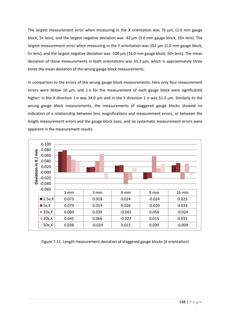
148 | P a g e
The largest measurement error when measuring in the X orientation was 79 µm, (1.0 mm gauge
block, 5× lens), and the largest negative deviation was -42 µm (3.0 mm gauge block, 10× lens). The
largest measurement error when measuring in the Y orientation was 102 µm (1.0 mm gauge block,
5× lens), and the largest negative deviation was -100 µm (16.0 mm gauge block, 50× lens). The mean
deviation of these measurements in both orientations was 33.3 μm, which is approximately three
times the mean deviation of the wrung gauge block measurements.
In comparison to the errors of the wrung gauge block measurements; here only four measurement
errors were below 10 µm, and 1 σ for the measurement of each gauge block were significantly
higher: in the X direction 1 σ was 34.0 μm and in the Y direction 1 σ was 51.0 μm. Similarly to the
wrung gauge block measurements, the measurements of staggered gauge blocks showed no
indication of a relationship between lens magnifications and measurement errors, or between the
length measurement errors and the gauge block sizes, and no systematic measurement errors were
apparent in the measurement results.
Figure 7.11: Length measurement deviation of staggered gauge blocks (X orientation)
1 mm 3 mm 4 mm 8 mm 16 mm2.5x,X 0.073 0.018 0.024 -0.024 0.0255x,X 0.079 0.019 0.026 -0.020 0.03310x,X 0.060 0.039 -0.042 0.058 -0.02420x,X 0.045 0.066 -0.027 0.015 0.03150x,X 0.038 -0.024 0.015 0.030 -0.009
-0.060-0.040-0.0200.0000.0200.0400.0600.0800.100
Devi
atio
n in
X /
mm
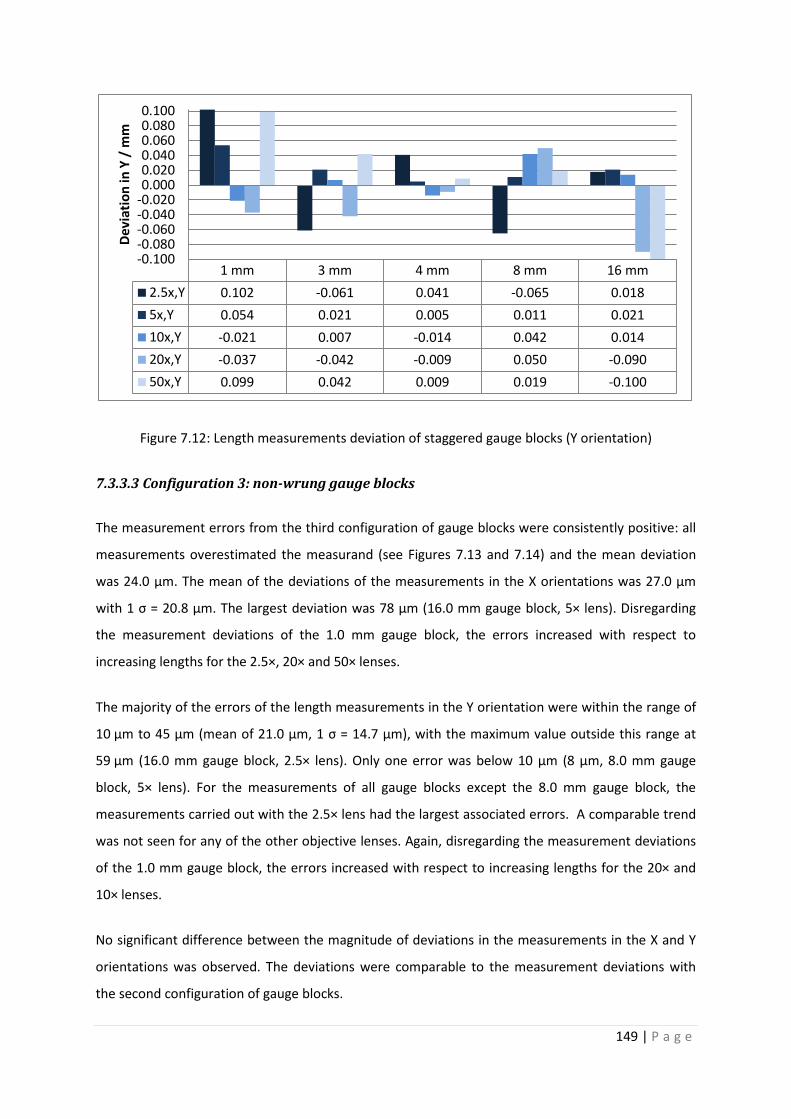
149 | P a g e
Figure 7.12: Length measurements deviation of staggered gauge blocks (Y orientation)
7.3.3.3 Configuration 3: non-wrung gauge blocks
The measurement errors from the third configuration of gauge blocks were consistently positive: all
measurements overestimated the measurand (see Figures 7.13 and 7.14) and the mean deviation
was 24.0 μm. The mean of the deviations of the measurements in the X orientations was 27.0 μm
with 1 σ = 20.8 μm. The largest deviation was 78 μm (16.0 mm gauge block, 5× lens). Disregarding
the measurement deviations of the 1.0 mm gauge block, the errors increased with respect to
increasing lengths for the 2.5×, 20× and 50× lenses.
The majority of the errors of the length measurements in the Y orientation were within the range of
10 µm to 45 µm (mean of 21.0 μm, 1 σ = 14.7 μm), with the maximum value outside this range at
59 µm (16.0 mm gauge block, 2.5× lens). Only one error was below 10 µm (8 μm, 8.0 mm gauge
block, 5× lens). For the measurements of all gauge blocks except the 8.0 mm gauge block, the
measurements carried out with the 2.5× lens had the largest associated errors. A comparable trend
was not seen for any of the other objective lenses. Again, disregarding the measurement deviations
of the 1.0 mm gauge block, the errors increased with respect to increasing lengths for the 20× and
10× lenses.
No significant difference between the magnitude of deviations in the measurements in the X and Y
orientations was observed. The deviations were comparable to the measurement deviations with
the second configuration of gauge blocks.
1 mm 3 mm 4 mm 8 mm 16 mm2.5x,Y 0.102 -0.061 0.041 -0.065 0.0185x,Y 0.054 0.021 0.005 0.011 0.02110x,Y -0.021 0.007 -0.014 0.042 0.01420x,Y -0.037 -0.042 -0.009 0.050 -0.09050x,Y 0.099 0.042 0.009 0.019 -0.100
-0.100-0.080-0.060-0.040-0.0200.0000.0200.0400.0600.0800.100
Devi
atio
n in
Y /
mm

150 | P a g e
Figure 7.13: Length measurement deviation of non-wrung gauge blocks (X orientation)
Figure 7.14: Length measurements deviation of non-wrung gauge blocks (Y orientation)
7.3.4 Conclusions and discussion
In the context of micro-CMMs, the length measurement errors presented here were very large. A
micro-CMM is expected to perform length measurements with uncertainties of less than 500 nm.
1 mm 3 mm 4 mm 8 mm 16 mm2.5x,X 0.027 0.003 0.022 0.035 0.0745x,X 0.038 0.002 0.022 0.004 0.07810x,X 0.032 0.005 0.019 0.017 0.03220x,X 0.014 0.012 0.02 0.023 0.05650x,X 0.018 0.016 0.019 0.017 0.057
00.010.020.030.040.050.060.070.08
Devi
atio
n in
X /
mm
1 mm 3 mm 4 mm 8 mm 16 mm2.5x.Y 0.045 0.031 0.038 0.016 0.0595x,Y 0.043 0.014 0.023 0.008 0.03310x,Y 0.026 0.011 0.012 0.0158 0.04120x,Y 0.028 0.012 0.015 0.026 0.03950x,Y 0.018 0.01 0.023 0.029 0.021
00.010.020.030.040.050.060.070.08
Devi
atio
n in
Y /
mm

151 | P a g e
The measurements of the wrung gauge block configuration had the smallest measurement errors
(mean = 10.1 μm) of all configurations, with smaller measurement deviations when measuring in the
Y orientation compared to the X orientation. These large measurement errors may have been
caused by sources listed in order of importance:
• the method of measuring the distance using the IFM G4 software that was primarily
designed for surface texture measurements (this includes human error);
• image stitching function (partly due to large black regions when measuring the staggered
gauge block configuration);
• inaccurate alignment of the profile perpendicular to the gauge block edges, causing a cosine
error (this error could have influenced the length measurement of the 16.0 mm gauge block
by 2.4 μm if the angle was misaligned by 1 degree); and
• measurement uncertainty of the instrument.
The gauge blocks in configurations two and three were not wrung, and therefore, it was expected
that the measurement deviations would be comparable. However, the results showed that, although
the measurement deviations were in general larger than the measurement deviations of wrung
gauge blocks (mean = 10.1 μm), they were not comparable. The mean measurement deviations of
staggered gauge blocks was 33.3 μm, and the mean measurement deviations of non-wrung, non-
staggered gauge blocks was 24.0 μm.
This disagreement between the expectation and the experimental evidence could be due to the
error caused by an insufficient amount of information provided for the stitching in places where the
gauge blocks were set back in the second configuration. Another error source for the length
measurements was the inaccuracy of edge measurement of the gauge blocks: the co-ordinate of a
point is calculated by taking the neighbouring pixels into account, at an edge however, half of the
neighbouring pixels do not give any information (except noise), which impairs the accuracy of the
edge location calculation. The large errors of the non-wrung gauge block measurements were partly
accounted for by the separation between each gauge block, despite the use of a gauge block clamp.
A conclusion that could be drawn from the results of all measurement methods was that the errors
did not relate to the magnification of the objective lenses. The reason for expecting a relationship
was because the area used for stitching of two images was larger for measurements carried out with
the 2.5× objective lens than higher magnification objective lenses with smaller FoVs, hence providing
more data for the image stitching function.

152 | P a g e
In the context of FV micro-CMMs, the measurement results of staggered gauge blocks showed the
importance of collecting sufficient data within each FoV when using the image stitching function.
The results of measuring the staggered gauge blocks also showed that for the development of a FV
micro-CMM an improvement of edge measurements is of importance and, therefore, an edge
detection function should be offered, using for example the Canny edge detection method
(Baehnisch et al. 2009).
With respect to a re-verification of a FV micro-CMM using prismatic shapes, the results obtained by
length measurement of wrung gauge blocks showed that a large measurement variation (1 σ =
17.9 μm) would have to be associated with the measurement results. This measurement variation
exceeded the expected uncertainty budget of a FV instrument. Therefore, the conclusion can be
drawn that prismatic shapes, such as gauge blocks, are not suited as a re-verification object for FV
micro-CMMs in the context of an IFM G4 instrument; artefacts without sharp edges are potentially
better suited for re-verification artefacts for a FV micro-CMM.
7.4 Spheres
7.4.1 Introduction
A key element of the current research is to develop suitable acceptance, re-verification and health
check procedures for a FV micro-CMM and to identify a suitable re-verification artefact, based on the
exploration of the applicability of the FV technique. An important issue with FV is that any reference
artefact must have a certain level of surface roughness (approximately Ra of 30 nm) (Danzl et al.,
2011) for the FV sensor system to work effectively.
The measurements of spheres presented here was one step in the development of a re-verification
artefact specifically for the assessment of length measurement error of FV micro-CMMs. The
investigation took into consideration surface roughness of spheres, sphere materials, and sphere
size. The aim here was to identify the most suitable material, the most suitable surface roughness
(and the method of roughening), the most suitable sphere diameter (2.0 mm, 1.0 mm or 0.5 mm),
and to investigate the effect of measurement area used for one measurement of the sphere radius.
7.4.2 Measurements of spheres
For the investigation of spheres the IFM G4 was used and the 50× magnification lens was chosen for
the majority of measurements in order to obtain comparable measurement results from spheres that
differed in material, surface roughness and diameter. The 10× objective lens was also used for

153 | P a g e
comparative measurements. The reason for having primarily chosen the 50× objective lens for the
majority of the work was because it fitted the criterion to challenge the IFM G4 instrument: its
associated half aperture angle was larger than that of lenses with lower magnifications, making a
larger high aspect ratio area of the spheres measurable, but the trade-off was the small FoV
compared to the surface area the sphere used.
The sphere materials used for this work were manufactured from aluminium oxide (ruby) (from
Renishaw), zirconia (from Saphirwerk Industrieprodukte AG), silicon nitride (from the Interstaatliche
Hochschule fuer Technik Buchs (NTB)) and stainless steel (from Simply Bearings Ltd). The ruby
spheres were chosen because they could be purchased mounted on styli, which facilitated their
handling. Silicon nitride spheres were used because of the contrast inherent in their surfaces.
Zirconia spheres were used because they offered a good balance between cost and roundness. The
stainless steel spheres were cheap, their quality lower, and therefore, their surface had some
roughness, which could be beneficial to their measurements.
The test spheres had nominal diameters of 2.0 mm, 1.0 mm and 0.5 mm, which were chosen
according to the FoV of the 50× lens (0.286 mm × 0.218 mm, the diagonal being 0.359 mm). When
centring the FoV with the top of the sphere, the maximum measurable percentage of the sphere’s
upper semi-circle was 5.7 % for the 2.0 mm diameter sphere, 11.5 % for the 1.0 mm diameter
sphere, and 42 % for the 0.5 mm diameter sphere. The amount of information gathered with one
FoV of the 2.0 mm diameter sphere was not ideal for a sphere-fitting operation, because it only
covered a small angle of the sphere’s circumference. In comparison, a larger per cent of a 0.5 mm
diameter sphere’s surface could be measured with one FoV, which could potentially be beneficial for
the sphere-fitting procedure.
ISO 3290 documents (ISO 3290-1, 2006; ISO 3290-2, 2008) exist for the standardisation of sphere
quality. Spheres are graded numerically from Grade 3 to beyond Grade 200, the higher numbers
being associated with higher form deviation, diameter variation and surface roughness. The spheres
used here were in the range from Grade 3 to Grade 100, with details given in Table 7.4 for each
sphere size and material.

154 | P a g e
Table 7.4: Specification of sphere qualities
Nominal
diameter
(mm)
Material Grade
Diameter
variation
(μm)
Deviation from
spherical form
(μm)
Roughness, Ra
(μm)
1.0 Ruby 5 0.13 0.13 0.014
1.0 Zirconia 3 0.08 0.08 0.010
1.0 Silicon nitride 5 0.80 0.13 0.018
1.0 Stainless steel 100 2.50 2.50 0.100
2.0 Zirconia 5 0.13 0.13 0.014
0.5 Zirconia 3 0.08 0.08 0.010
The following experiments were conducted for the measurement of the spheres:
1. Comparison of size measurements between all four materials using 1.0 mm diameter
spheres;
2. Assessment of the effect on size measurement when etching 1.0 mm ruby spheres;
3. Assessment of the effect on size measurement when etching 1.0 mm zirconia spheres using
three different measurement procedures (single images, image field and edited image field);
4. Comparison of size measurement accuracy between differently sized spheres, using zirconia
spheres with 2.0 mm, 1.0 mm and 0.5 mm diameters;
5. Comparison of size measurements using only one FoV and multiple FoVs for one
measurement, using 1.0 mm stainless steel spheres;
6. Assessment of measurement variation introduced by the measurement process and by the
sphere-fitting operation.
The measurement procedure for each of the spheres regardless of the material and size was as
follows.
• The sphere was placed into a holder in the measuring volume and the scan length (Z axis
travel) and settings (specific for each measurement) adjusted, using a 50× magnification lens
(unless indicated otherwise).
• The top hemi-sphere of each sphere was measured three times to retrieve 3D models of the
surface using either one FoV or multiple FoVs with the image stitching option.

155 | P a g e
• A robust sphere-fitting operation, based on a Gaussian best-fit algorithm, was applied to the
effective surface five times repeatedly, and the radii of the five fitted (virtual) spheres were
recorded.
7.4.2.1 Comparison of different sphere materials
The first set of measurements was of 1.0 mm spheres of all four materials in order to compare the
suitability of the materials to measurements with the FV technique. These spheres were off-the-shelf
products and were not modified for this experiment; hence their specifications in Table 7.4 are
relevant. The measurement procedure did not alter from the description given above and the
measurement settings specific for each material is given in Table 7.5. It was found that for the
measurement of ruby spheres a lower magnification (and consequently lower resolution) was
necessary in order to obtain more contrasted images, and the 10× lens was used.
Table 7.5: Sphere measurement settings for each material
Setting Units Ruby sphere Zirconia sphere Silicon nitride Stainless Steel
Lens magnification - 10× 50× 50× 50×
Exposure time (μs) 2,349 391 725 593
Coaxial light, intensity (%) 7 100 20 20
Ring-light, intensity (%) 100 Deactivated Deactivated Deactivated
Contrast - 0.7 3.3 0.6 1.2
Lateral resolution (μm) 3.9 2.1 2.1 2.1
Vertical resolution (nm) 362 103 329 104
Polariser - Activated Deactivated Deactivated Deactivated
7.4.2.2 Etching ruby spheres
The second experiment was initiated as a function of the poor outcome of the first set of
measurements: the highly reflective ruby surfaces required preparation to provide a higher degree of
surface roughness than unprepared ruby spheres. The aim here was to investigate how etching of
ruby spheres affected the measurement quality.
Twenty synthetic ruby spheres were etched in an unstirred bath of weak (1 %) hydro-fluoric (HF) acid
with etching times ranging from 5 minutes to 100 minutes with 5 minute increments. The spheres

156 | P a g e
were washed off immediately with water and dried with hot air. The measurement settings used for
each sphere were the same as given in Table 7.5.
For comparison reasons these ruby spheres were measured with the Zeiss F25 (see Chapter 2) at the
NPL. The measurements with the Zeiss F25 were conducted in a temperature (20 °C ± 0.5 °C) and
humidity (50 % ± 10 % rH) controlled environment. Four spheres (etching times: 0 minutes,
15 minutes, 55 minutes and 100 minutes) were measured three times repeatedly without rotating
the sphere between each measurement. For each measurement four points were measured at
approximately 90 degree intervals around the sphere’s equator, four points at approximately 45
degrees from the sphere’s equator towards the top (also at approximate intervals of 90 degrees) and
one point at the top.
7.4.2.3 Etching zirconia spheres
For the third investigation, zirconia spheres were etched with different etching times in order to
create different levels of roughness on the spheres’ surfaces that would provide more contrast for
surface measurements with the FV technique. The aim of this investigation was to explore the
relationship between the etching times and the measurement quality, to explore the affect of using
an image field compared to a single FoV on the radius measurement, and to explore the affect of the
spike-removal editing function on the radius measurements.
The etching process of six 1.0 mm zirconia spheres was carried out with a 6 % HF acid at room
temperature and with etching times ranging from 10 minutes to 40 minutes with 5 minutes
increments. Similarly to the etching procedure of ruby spheres, the HF acid was not stirred whilst the
spheres were being etched, and the spheres were washed off immediately with water and dried with
hot air.
Each sphere radii were measured with three methods as follows (the measurement settings are
given in Table 7.6.).
• The spheres were measured three times repeatedly using only one FoV.
• The spheres were measured with an image field of 3×3 FoVs (10 % overlap).
• The latter set of data was additionally processed with a spike removal function offered in the
IFM G4’s software.

157 | P a g e
The editing process was carried out to assess the effect of noise in terms of spikes on sphere
measurements, for which the raw measurement data sets were once directly used for the sphere
fitting operation and a second time run through a spike removal operation before the sphere fitting
operation. The radius of each effective surface was measured five times repeatedly by using a robust
Gaussian sphere-fitting function in Alicona’s surface texture software, that does not take outliers into
account.
Additionally, the sphere roughness was also recorded in terms of Ra, using a cut-off value of 80 μm
and five line profiles over the surface of the spheres, in order to explore a possible relationship
between the measurement quality and the surface’s roughness.
Table 7.6: Measurement settings of zirconia spheres
Setting Units Single FoV Multiple FoVs
Lens magnification - 50× 50×
Exposure time (μs) 365 411
Coaxial light, intensity (%) 100 100
Ring-light, intensity (%) 0 0
Contrast - 2.61 2.52
Lateral resolution (μm) 2.1 2.1
Vertical resolution (nm) 41 70
Polariser - Deactivated Deactivated
7.4.2.4 Using differently sized spheres
The fourth set of measurements aimed to assess how the sphere size affects the measurement
quality. Three non-etched zirconia spheres (2.0 mm, 1.0 mm and 0.5 mm) were measured three
times each, producing three effective surfaces, to each of which five virtual spheres were fitted. The
measurement settings are given in Table 7.7.

158 | P a g e
Table 7.7: Sphere measurement settings for each zirconia sphere size
Setting Units 2.0 mm 1.0 mm 0.5 mm
Lens magnification - 50× 50× 50×
Exposure time (μs) 504 391 743
Coaxial light, intensity (%) 58 100 57
Ring-light, intensity (%) 90 0 100
Contrast - 2.7 3.3 2.0
Lateral resolution (μm) 1.6 2.1 2.1
Vertical resolution (nm) 87 41 104
Polariser - Deactivated Deactivated Deactivated
7.4.2.5 Single FoV versus multiple FoVs
Stainless steel spheres were measured with a single FoV and multiple FoVs (3 × 3, overlap: 10 %),
with the aim to explore the effect of the size measurement on the radius measurement of a sphere.
The measurement procedure, as specified in Section 7.4.2, was completed with the settings given in
Table 7.8.
Table 7.8: Sphere measurement settings for stainless steel spheres
Setting Units Single FoV Multiple FoVs
Lens magnification - 50× 50×
Exposure time (μs) 593 229
Coaxial light, intensity (%) 20 100
Ring-light, intensity (%) 0 0
Contrast 1.2 0.8
Lateral resolution (μm) 2.1 2.1
Vertical resolution (nm) 104 300
Polariser - Deactivated Deactivated
7.4.2.6 Variation of measurements
The last assessment of sphere measurements was conducted in order to separate the measurement
variation introduced by the data collection process and the variation introduced by the sphere-fitting

159 | P a g e
operation. For this assessment existing measurements of 1.0 mm stainless steel spheres were used
that have been obtained with multiple FoVs.
Because the process of measuring the sphere’s radius involved a hardware and software procedure,
the measurement repeatability and variation introduced by the sphere-fitting function could not be
entirely separated: the variation due to the data collection process was quantified by the standard
deviation of the averaged repeated radius measurements of three effective surfaces, and the
variation due to the sphere-fitting operation was quantified by the standard deviation of radius
measurements by repeated sphere-fitting operations on a single effective surface. To facilitate the
understanding of the above, the following image (Figure 7.15) is included, which visualises the data
used to obtain the mean of standard deviations and the standard deviation of mean standard
deviations.
Figure 7.15: Evaluation of sphere measurement results

160 | P a g e
7.4.3 Results of sphere measurements
7.4.3.1 Comparison of different sphere materials
Figure 7.16(a-d) shows the results of radius measurements of four non-etched 1.0 mm spheres of
four different materials. These results will be discussed in two parts: firstly from a qualitative point of
view and secondly from a quantitative point of view.
From a qualitative perspective, it was found that the measurement of the ruby sphere contained a
very large amount of spikes and data holes. It was found that the data collected from the ruby sphere
was very poor, due to the reflective and transparent nature of the sphere’s surface. The latter
characteristic of ruby spheres caused internal reflections from within the sphere. Changing to a 10×
lens magnification offered a lower lateral resolution (3.9 μm), generating higher contrast within each
image that was used for the reconstruction of the effective surface. Despite the change of objective
lens magnification, the effective surface contained a lot of noise and data loss.
Zirconia spheres were measured without major spikes but data was missing at the edges of the
images, where the surface curvature increased. It was also observed that there were patches of
smooth and featureless data areas (shown in the Figure 7.16(b) as small dark patches), which
indicated that the surface roughness may have been below the ideal measurement criterion for the
technique.
The silicon nitride sphere measurements produced effective surfaces that did not feature visible
noise or missing data. The surface representation was continuous, without any data loss or spikes.
The surface representation of the stainless steel sphere measurements compared well to that of the
silicon nitride sphere in terms of data continuity. However, unlike the silicon nitride sphere
measurements, the effective surfaces of the stainless steel spheres featured visible surface
undulation, which indicated the presence of waviness, and which may correlate with the grade 100
specifications of the spheres.

161 | P a g e
Figure 7.16: Surface representation of (a) ruby, (b) zirconia, (c) silicon nitride, (d) stainless steel
The numerical evaluation, presented in Table 7.9 and Figure 7.17, of the measurements showed that
the ruby and zirconia spheres each had a diameter of 507 μm, but the standard deviation associated
with the ruby sphere was 20.4 μm, whilst the zirconia sphere was measured with a standard
deviation of 0.8 μm (4 % of the ruby standard deviation). The silicon nitride sphere’s diameter was
measured to be 504 μm with a standard deviation of 2.3 μm and the stainless steel sphere had a
measured diameter of 501 μm, with a standard deviation of 3.3 μm. The measured stainless steel
sphere diameter was closest to the nominal value of 500 μm, followed by the silicon nitride sphere.
The silicon nitride sphere measurement featured a highly contrasted surface. This contrast was only
partially caused by the surface’s roughness; the natural variation of chemical composition within the
material caused colour differences within the bulk material, consequently causing contrasted surface
areas, and thus a nano-roughness was less important. The repeated measurement of the zirconia
spheres had a small spread of results (1 σ = 0.8 μm). This indicated very repeatable constructions of
effective surfaces as well as very good repeatability of the sphere fitting procedure.
Table 7.9: Measured radii of 1.0 mm diameter spheres
Material Measured radius
(μm)
Standard deviation
(μm)
Ruby 507 20.4
Zirconia 507 0.8
Silicon nitride 504 2.3
Stainless steel 501 3.3

162 | P a g e
Figure 7.17: Radius measurement of 1.0 mm spheres
7.4.3.2 Etching ruby spheres
The results of the previous set of measurements showed that ruby (as manufactured for CMM styli)
was not suitable for FV instruments. Therefore, 1.0 mm ruby spheres underwent an etching process
in order to produce a series of etched spheres. The measured radii of all etched spheres are shown in
Figure 7.18. The results could be split into two brackets of etching times. At 0 minutes to 65 minutes
the radii had deviations below 10 μm with two exceptions at 30 and 40 minutes. At 70 minutes to
100 minutes, only two measurements had a deviation of less than 10 μm from the nominal. All other
deviations were within the range of 14 μm to 67 μm. For this second bracket of etching times the
spread of radius measurements was 100.9 μm. In general, the longer the ruby sphere had been
etched, the more likely their measured radius was to deviate strongly (more than 10 μm) from the
nominal value.
It was expected that the etching process would roughen the surfaces, giving them contrasted
roughness and opaque surface characteristics, and thus making them more suitable for
measurements with the FV technique. The expectation was that the etched sphere radii would be
measured more closely to 500 μm and with smaller uncertainties. This expectation was not met by
the measurement results that can be seen in Figure 7.18.
507 507 504 501
480
490
500
510
520
530
Ruby Zirconium Silicon Nitride Stainless Steel
Radi
us /
µm
Materials

163 | P a g e
Figure 7.18: Size measurements of 1.0 mm etched ruby spheres
Repeated measurements performed with the F25 micro-CMM showed that the radius deviations
from the nominal were not as large as measured on the IFM G4. The non-etched sphere was
measured with a radius of 501 μm, and the radii of the etched spheres were 500.5 μm, 500.1 μm,
and 500.5 μm respectively for the 15 minutes, 55 minutes and 100 minutes etched spheres. These
results are shown in Figure 7.19 together with their standard deviations, of which the largest was
associated with the 15 minute etched sphere and was 92 nm.
Replacing the nominal values, specified by the sphere manufacturer, by the measurement results of
the F25, the size measurement deviation of the radius measurement with the IFM G4 was less than
6 μm. The other size measurement deviations measured with the IFM G4 of the spheres etched for
15 minutes, 55 minutes and 100 minutes were then 7.4 μm, 2.9 μm and 7.4 μm respectively.
509.3 507.8 506.6 504.9
521.8
502.6
533.4
495.9
505.4 502.8 506.6
500.0
465.6
505.4
525.3
514.0
566.5
483.2
493.1
460
480
500
520
540
560
0 10 20 30 40 50 60 70 80 90 100
Radi
us /
μm
Etching time / minutes

164 | P a g e
Figure 7.19: Size measurements of 1.0 mm etched ruby spheres with the Zeiss F25
The measurements with the Zeiss F25 of the non-etched, the 15 minute and 55 minute etched
spheres show a relationship between the etching time and the measured radius: the longer the
spheres were etched the smaller they became. However, the measurement of the 100 minute
etched sphere has a larger radius than the 55 minute etched sphere, which is an observation that
does not support the expected relationship between the etching time and the sphere size. The
reason for this may have been the synthetic nature of the ruby spheres, which meant that the
crystalline structure may have had internal strains or imperfections (Mukherjee, 2011). Where the
sphere surface was imperfect, the HF acid was likely to etch away the aluminium oxide quicker,
causing variations in the etching over the sphere's surface.
Etching ruby spheres improved measurability, but did not significantly improve the overall results,
because the etching process did not occur homogeneously on the whole surface, instead
concentrated on particular areas, possibly where the crystal structure featured defects. Therefore, it
was concluded that ruby spheres should not be considered as part of a re-verification artefact
because they cannot be measured accurately and precisely even after undergoing an etching
procedure.
7.4.3.3 Etching zirconia spheres
The results of etched zirconia spheres are presented and discussed individually before the three sets
of results are compared to identify correlations between the data sets. The results, shown in
Table 7.10 and Figure 7.20, of measurements performed with a single FoV showed no particular
trend. Figure 7.21 shows an effective surface of the 20 minute etched sphere. Most of the
measurements were within 0 μm to 8 μm deviation band. Only the measurement of the 40 minute
etched sphere deviated from the nominal by 13.2 μm. The standard deviation of all 15 values per
501.3
500.5
500.1
500.5
500
500.5
501
501.5
0 10 20 30 40 50 60 70 80 90 100
Radi
us /
μm
Etching time / minutes

165 | P a g e
sphere showed no correlation with the etching time: the sphere etched for 10 minutes had the
largest standard deviation with 4.7 μm, which may be an outlier, followed by the 35 minute etched
sphere with 1σ = 3.6 μm. The smallest standard deviation (0.6 μm) was associated with the
20 minute etched sphere, which simultaneously had the smallest size measurement deviation of
0.5 μm from the nominal radius value. The non-etched sphere was measured to have a radius
deviation of 7.5 μm, which was larger than the measured deviation of the spheres etched for
10 minutes, 15 minutes, 20 minutes, and 25 minutes. The results indicated that etching zirconia
spheres for 20 minutes may produce an ideal surface roughness to make them more accurately
measurable with a FV technique.
Table 7.10: Measured radii of 1.0 mm etched zirconia spheres (single FoV)
Etching time
(minutes)
Measured radius
(μm)
Standard deviation
(μm)
0 507.5 0.8
10 502.6 4.7
15 503.6 1.2
20 500.5 0.6
25 501.4 1.9
35 507.8 3.6
40 513.2 2.0
Figure 7.20: Measured radii of 1.0 mm etched zirconia spheres (single FoV)
507.5
502.6 503.6 500.5 501.4
507.8
513.2
490.00
495.00
500.00
505.00
510.00
515.00
520.00
525.00
0 5 10 15 20 25 30 35 40
Radi
us /
μm
Etching time / minutes

166 | P a g e
Figure 7.21: 1.0 mm zirconia sphere etched for 20 minutes (single FoV)
The expectation of this data set was a diminishing of radius deviation from the nominal with
increasing etching time. What was seen in the results, however, were deviations (including ±1 σ)
equal or smaller than 5 μm ( = 1 % error of the nominal radius) for the spheres etched for 15 minute,
20 minute, and 25 minute durations. For the 10 minute, 35 minute and 40 minute etched spheres
the measurement deviation was above 5 μm. It was also expected that the standard deviation of the
measurements of each sphere would decrease with increasing etch time, because it was expected
that more pits would be etched into the surface causing the surface to be more contrasted. This
expectation was not met by the results either: the largest deviation was associated with the
10 minute etched sphere.
The results lead to the question: Why was the smallest deviation achieved at an etch time of
20 minutes and not at a longer etching time? There may be several reasons for this occurrence:
either 20 minutes may have been the etch time to establish a roughness that scatters light very well,
and produces a well contrasted image; or this particular sphere had the smallest radius of all etched
spheres before it was etched and the variation in measured radii represented the variation in the
sphere manufacturing; or this sphere coincidentally had a particularly homogeneous surface that
was repeatedly measureable (with very little optical noise).
There were two conclusions that could be drawn from this set of measurements: one conclusion
that does not take the standard deviations into account, and the other conclusion that takes the
standard deviation into account. The first conclusion was that the etching times that produced the
ideal surface roughness were in the range of 10 minutes to 25 minutes, and secondly conclusion was
that the effect of etching did not achieve the desired effect on the accuracy and precision of sphere
measurements. The second conclusion was drawn due to the non-predictable spread of values, i.e.
the associated standard deviations were very large.

167 | P a g e
The same spheres have also been measured using an image field of 3 × 3 FoV with a 10 % overlap
and the results of these measurements are presented in Table 7.11 and Figure 7.22. An effective
surface is depicted in Figure 7.23. Only the measured mean radius plus two standard deviations
associated with the sphere measurement that was etched for 35 minutes was within 5 μm from the
nominal value. All other sphere measurements included data points outside the ± 5 μm band around
the nominal value (= 1 % error). Regarding the measured mean radius of each sphere, four were
within the ± 5 μm band (10 minute, 15 minute, 20 minute and 35 minute etching times). The sphere
with the largest standard deviation (15.1 μm) was the sphere that was etched for 40 minutes: the
fifteen individual measurements showed that the reason for this large deviation was due to one of
the three effective surfaces that were measured having a much larger radius. Without taking this
singular effective surface into account, the mean radius (based on ten values) was 498.1 μm
(± 2.8 μm), placing the measurement within the 1 % error band. The sphere with the second largest
standard deviation was etched for 15 minutes and had the lowest radius measurement deviation
from the nominal 500 μm.
Table 7.11: Measurement data for 1.0 mm zirconia spheres (image field)
Etching time
(minutes)
Measured radius
(μm)
Standard deviation
(μm)
10 502.2 4.8
15 501.1 5.9
20 502.4 3.9
25 506.3 4.9
35 502.1 2.0
40 508.3 (498.1) 15.1 (2.8)
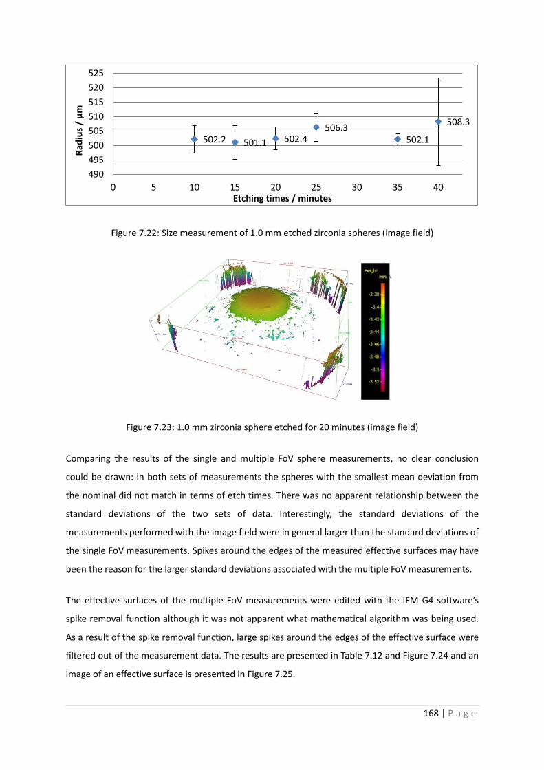
168 | P a g e
Figure 7.22: Size measurement of 1.0 mm etched zirconia spheres (image field)
Figure 7.23: 1.0 mm zirconia sphere etched for 20 minutes (image field)
Comparing the results of the single and multiple FoV sphere measurements, no clear conclusion
could be drawn: in both sets of measurements the spheres with the smallest mean deviation from
the nominal did not match in terms of etch times. There was no apparent relationship between the
standard deviations of the two sets of data. Interestingly, the standard deviations of the
measurements performed with the image field were in general larger than the standard deviations of
the single FoV measurements. Spikes around the edges of the measured effective surfaces may have
been the reason for the larger standard deviations associated with the multiple FoV measurements.
The effective surfaces of the multiple FoV measurements were edited with the IFM G4 software’s
spike removal function although it was not apparent what mathematical algorithm was being used.
As a result of the spike removal function, large spikes around the edges of the effective surface were
filtered out of the measurement data. The results are presented in Table 7.12 and Figure 7.24 and an
image of an effective surface is presented in Figure 7.25.
502.2 501.1 502.4 506.3
502.1
508.3
490495500505510515520525
0 5 10 15 20 25 30 35 40
Radi
us /
µm
Etching times / minutes

169 | P a g e
The results showed that the spheres with the smallest radius measurement deviations from the
nominal value were etched for 35 minutes and 40 minutes. The first of these measurements had the
smallest standard deviation (1.6 μm), whilst the latter measurement value was associated with the
largest standard deviation (6.7 μm) of this data set. This large standard deviation was (similarly to the
equivalent non-edited measurement result) due to one of the three measured effective surfaces,
without which the standard deviation calculated from ten values would be approximately halved
(3.5 μm). All but one mean radius measurement value lay within the 1 % deviation band but all data
values were contained in the 2 % error band (equivalent to 10 μm error from the nominal radius).
Table 7.12: Measured radii of 1.0 mm etched zirconia spheres (image field, spike removal)
Etching time
(minutes)
Measured radius
(μm)
Standard deviation
(μm)
10 503.0 5.3
15 502.5 5.1
20 504.7 3.0
25 505.7 3.9
35 501.7 1.6
40 501.8 6.7
Figure 7.24: Measured radii of 1.0 mm etched zirconia spheres (image field, spike removal)
503.0 502.5 504.7 505.7
501.7 501.8
490
495
500
505
510
515
520
525
0 5 10 15 20 25 30 35 40
Radi
us /
μm
Etching times / minutes

170 | P a g e
Figure 7.25: 1.0 mm zirconia sphere etched for 20 minutes (image field, spike removal)
The effect of filtering out large spikes from an effective surface can be analysed by comparing the
non-edited and the edited measurement results. Here the 40 minute etched sphere provided the
biggest difference: the editing process lowered the radius deviation considerable (6.7 μm) and
diminished the standard deviations by 55 % on average. This effect, however, was not so apparent
for the measurement of the other three spheres: three measurements showed larger radius
deviations after the editing process (10 minute, 15 minute and 20 minute etching time) and in two
cases the errors were smaller after editing (25 minute and 35 minute etching time).
Comparing the edited multiple FoV measurement set to the single FoV measurement set, it was
noticeable that the radius deviations were more spread out for the single FoV measurements and
that the standard deviations of the measurements were in general smaller. The latter observation
may have meant that the sphere fitting procedure using less data could be completed in a more
repeatable manner.
The Ra roughness values of the effective surfaces measured with multiple FoVs of all etched spheres
were calculated with the aim to find a relationship between the roughness and the radius deviations
from the nominal. The Ra roughness values are presented in Table 7.13 and Figure 7.26. It was found
that the roughness of all spheres were in the range of 39 nm to 48 nm. This is a spread of only 9 nm,
which in the context of surface roughness is not very large. The surface roughness of the 10 minute
etched zirconia sphere was the lowest, followed by the 20 minute etched sphere with 40 nm. The
highest roughness was measured for the 35 minute etched sphere. The 15 minute, 25 minute and 40
minute etched spheres did not have noticeably higher or lower roughness values. Most of the
measurement standard deviations were approximately 5 nm, the smallest value being 1.2 nm for the
20 minute etched sphere.

171 | P a g e
Comparing all radius measurements with the roughness measurements of the etched spheres, there
was no apparent relationship between the measured sphere’s roughness and the radius deviations.
Table 7.13: Roughness values of all etched 1.0 mm zirconia spheres
Etching time
(minutes)
Measured roughness, Ra
(nm)
Standard deviation
(nm)
10 39 5.5
15 46 7.0
20 40 1.2
25 45 2.6
35 48 5.9
40 43 4.9
Figure 7.26: Roughness (Ra) of etched 1.0 mm zirconia spheres (image field measurements)
7.4.3.4 Using differently sized zirconia spheres
The measurements of differently sized zirconia spheres were compared to each other by means of
measurement one standard deviation. The three spheres diameter sizes were 2.0 mm, 1.0 mm, and
0.5 mm. The expectation was that the measured radii of the spheres would have a balanced
distribution of positive and negative radius deviations. The results showed that for each size the
measured radii of the three spheres were either all positive or all negative: the 2.0 mm spheres were
measured with a negative deviation from the nominal, and the 1.0 mm and 0.5 mm sphere were
measured with positive deviations. The data is presented in Tables 7.14 to 7.16 and in Figures 7.27 to
7.29 with illustrations of the effective surface in Figures 7.30 to 7.32.
39
46
40 45
48 43
30354045505560
0 5 10 15 20 25 30 35 40
Ra /
nm
Etching time / minutes

172 | P a g e
Table 7.14: Measured radii of 2.0 mm zirconia spheres (one FoV)
Sphere number Measured radius
(μm)
Standard deviation
(μm)
Mean standard deviation
(μm)
1 992.1 18.4
11.9 2 989.9 10.8
3 990.9 6.5
Table 7.15: Measured radii of 1.0 mm zirconia spheres (one FoV)
Sphere number Measured radius
(μm)
Standard deviation
(μm)
Mean standard deviation
(μm)
1 512.3 3.0
2.38 2 507.2 1.6
3 507.9 2.5
Table 7.16: Measured radii of 0.5 mm zirconia spheres (one FoV)
Sphere number Measured radius
(μm)
Standard deviation
(μm)
Mean standard deviation
(μm)
1 253.3 2.4
2.58 2 252.4 2.3
3 256.2 3.0
Figure 7.27: Measured radii of 2.0 mm spheres (one FoV)
992.1 989.9 990.9
970
980
990
1000
1010
1020
0 1 2 3
Radi
us /
μm
Sphere number
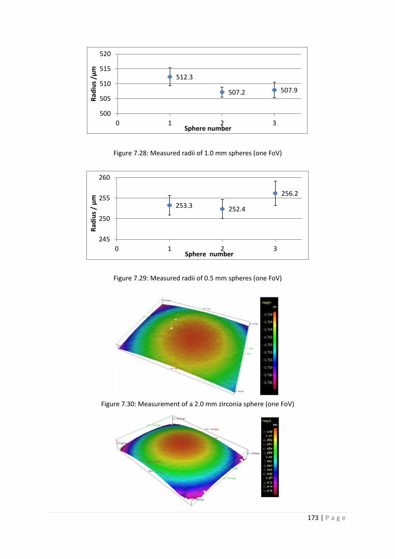
173 | P a g e
Figure 7.28: Measured radii of 1.0 mm spheres (one FoV)
Figure 7.29: Measured radii of 0.5 mm spheres (one FoV)
Figure 7.30: Measurement of a 2.0 mm zirconia sphere (one FoV)
512.3
507.2 507.9
500
505
510
515
520
0 1 2 3
Radi
us /
μm
Sphere number
253.3 252.4
256.2
245
250
255
260
0 1 2 3
Radi
us /
μm
Sphere number

174 | P a g e
Figure 7.31: Measurement of a 1.0 mm zirconia sphere (one FoV)
Figure 7.32: Measurement of a 0.5 mm zirconia sphere (one FoV)
When comparing the error percentage of size deviation it was found to be correlated with the sphere
size. The mean radius measurement deviations of the 2.0 mm spheres was equivalent to a 3.6 %
error, the mean error percentage of the 1.0 mm spheres was 1.8 % and that of the 0.5 mm spheres
was 1.5 %. This result may be explained by the amount of data collected for each measurement in
comparison to the sphere size. For all of the measurements the 50× objective lens was used, which
has a FoV of 0.289 mm by 0.218 mm (diagonal of 0.359 mm). Using simple geometry, as shown in
Figure 7.33 (where D is the image diagonal, r the sphere radius, and θ half the maximum angle) and
the information given about the FoV and the sphere size, the maximum angle of a measureable arc
on the sphere’s surface was calculated and presented in Table 7.17.
Figure 7.33: Calculating the maximum angle covered by the FoVs diagonal
Table 7.17: Maximum angle of an arc measurable by one FoV using the 50× objective lens
Sphere radius
(mm)
Angle, 2*θ
(degrees)
1.00 20.7
0.50 42.2
0.25 91.9
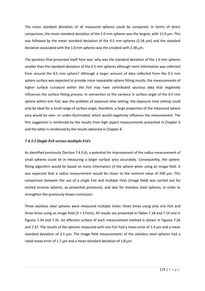
175 | P a g e
The mean standard deviation of all measured spheres could be compared. In terms of direct
comparison, the mean standard deviation of the 2.0 mm spheres was the largest, with 11.9 μm. This
was followed by the mean standard deviation of the 0.5 mm spheres (2.58 μm) and the standard
deviation associated with the 1.0 mm spheres was the smallest with 2.38 μm.
The question that presented itself here was: why was the standard deviation of the 1.0 mm spheres
smaller than the standard deviation of the 0.5 mm spheres although more information was collected
from around the 0.5 mm sphere? Although a larger amount of data collected from the 0.5 mm
sphere surface was expected to provide more repeatable sphere fitting results, the measurements of
higher surface curvature within the FoV may have contributed spurious data that negatively
influences the surface fitting process. In connection to the variance in surface angle of the 0.5 mm
sphere within one FoV, was the problem of exposure time setting: the exposure time setting could
only be ideal for a small range of surface angle, therefore, a large proportion of the measured sphere
area would be over- or under-illuminated, which would negatively influence the measurement. The
first suggestion is reinforced by the results from high aspect measurements presented in Chapter 6
and the latter is reinforced by the results obtained in Chapter 4.
7.4.3.5 Single FoV versus multiple FoVs
As identified previously (Section 7.4.3.4), a potential for improvement of the radius measurement of
small spheres could lie in measuring a larger surface area accurately. Consequently, the sphere-
fitting algorithm would be based on more information of the sphere when using an image field. It
was expected that a radius measurement would be closer to the nominal value of 500 μm. This
comparison between the use of a single FoV and multiple FoVs (image field) was carried out for
etched zirconia spheres, as presented previously, and also for stainless steel spheres, in order to
strengthen the previously drawn conclusion.
Three stainless steel spheres were measured multiple times: three times using only one FoV and
three times using an image field (3 × 3 FoVs). All results are presented in Tables 7.18 and 7.19 and in
Figures 7.34 and 7.35. An effective surface of each measurement method is shown in Figures 7.36
and 7.37. The results of the spheres measured with one FoV had a mean error of 1.4 μm and a mean
standard deviation of 3.1 µm. The image field measurements of the stainless steel spheres had a
radial mean error of 1.7 μm and a mean standard deviation of 1.8 µm.
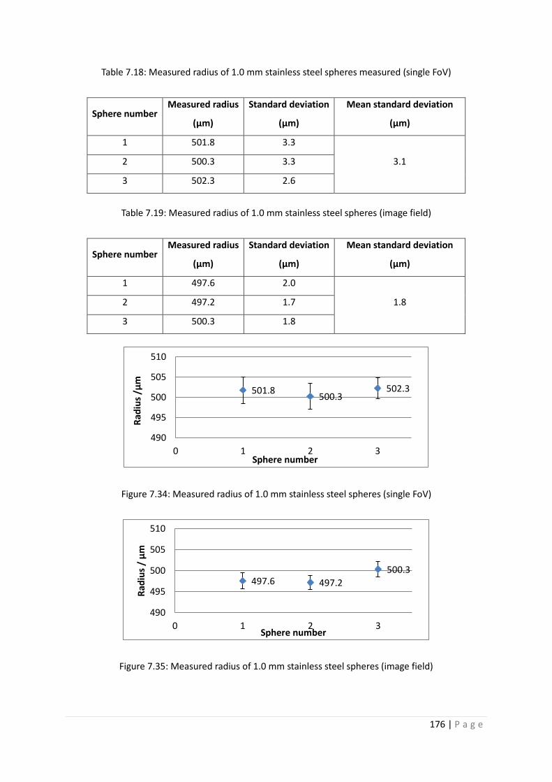
176 | P a g e
Table 7.18: Measured radius of 1.0 mm stainless steel spheres measured (single FoV)
Sphere number Measured radius
(μm)
Standard deviation
(μm)
Mean standard deviation
(μm)
1 501.8 3.3
3.1 2 500.3 3.3
3 502.3 2.6
Table 7.19: Measured radius of 1.0 mm stainless steel spheres (image field)
Sphere number Measured radius
(μm)
Standard deviation
(μm)
Mean standard deviation
(μm)
1 497.6 2.0
1.8 2 497.2 1.7
3 500.3 1.8
Figure 7.34: Measured radius of 1.0 mm stainless steel spheres (single FoV)
Figure 7.35: Measured radius of 1.0 mm stainless steel spheres (image field)
501.8 500.3 502.3
490
495
500
505
510
0 1 2 3
Radi
us /
µm
Sphere number
497.6 497.2 500.3
490
495
500
505
510
0 1 2 3
Radi
us /
μm
Sphere number

177 | P a g e
Figure 7.36: Effective surface of 1.0 mm stainless steel spheres (single FoV)
Figure 7.37: Effective surface of 1.0 mm stainless steel spheres (image field)
The measurement variation of the image field measurements could be due to data loss and spikes
within the image field. When setting up the experiment to measure a large range of surface angle
(here 0 degrees to 45 degrees), the light setting becomes increasingly important: over-exposure of
the top of the sphere should be avoided as it causes noise in the results, which influences the sphere
fitting algorithm. However, a too short exposure time causes under-exposure of the sloped surfaces
and consequently data loss and spikes, by which poor data quality is defined, inherently causing a
sphere fitting procedure with large repeatability value. The effect of over- and under-exposure was
previously explored in Chapter 4, where it was found that under-exposure increases the noise level.
The polariser may have improved the measurement results, however, due to the time-penalty
connected with the use of the polariser, it was not used.

178 | P a g e
The amount of information gathered from the stainless steel spheres when using an image field
relied on the surface's micro-roughness. Chapter 6 on measurements of high aspect ratio surfaces
reported that effective surfaces of steep surfaces contained re-entrant features, where not enough
data was provided (see Figure 7.37). Potentially, these features could have been a source of error for
the form-fitting process of the multiple FoVs measurements.
The mean standard deviation of the measurements with multiple FoV was smaller (60 %) than the
mean standard deviation for single FoV measurements. The most likely reason for this outcome was
the smaller surface area that was used for the sphere-fitting procedure applied to the single FoV
measurements. The results showed that for measurements of grade 100 stainless steel spheres
multiple FoVs could be beneficial to halve the measurement variation of the sphere measurements.
The disadvantage to using an image field is the extended time duration for each sphere
measurement (3 minutes) in comparison to the single FoV sphere measurements (45 seconds).
7.4.3.6 Variation of measurements
The aim here was to separate the radius measurement repeatability and the variation potentially
caused by the sphere-fitting function, which was embodied and quantified by the standard deviation
of five repeated sphere-fitting procedures to an effective surface.
The mean of standard deviations of five measured radii was calculated for repeated measurements
(using an image field) of each of the three stainless steel sphere. The standard deviations of all five
fitted spheres to one effective surface had mean values of 2.07 μm, 1.69 μm and 1.73 μm, as shown
in Table 7.20 and Figure 7.38.
Table 7.20: Mean standard deviations of stainless steel spheres
Sphere number Mean of standard deviations
(μm)
Standard deviation of mean
(μm)
1 2.07 0.35
2 1.69 0.65
3 1.73 0.25

179 | P a g e
Figure 7.38: Mean standard deviations of five radii calculations (using stainless steel sphere
measurement data)
7.4.4 Discussion and conclusions
The ruby sphere experimentation provided a clear conclusion: the smooth and translucent surface of
the ruby sphere was not suited for measurements with a FV instrument. Conclusions for the other
sphere materials were based on the measurement standard deviations: the zirconia sphere was
measured with a small measurement variation; the silicon nitride sphere was measured with a larger
measurement variation in comparison to the zirconia sphere measurement; and the stainless steel
sphere was measured with the largest measurement variation.
It was noticed that the measured radii (Figure 7.16) of the ruby, zirconia and silicon nitride spheres
were larger than the nominal value of 500 μm. This raised the question as to whether or not the
spheres were all coincidentally slightly larger than the nominal indicated by each independent
manufacturer or whether it was due to the measurement and the robust sphere fitting algorithm of
the FV instrument (Forbes, 1989). Each of the spheres had a diameter tolerance (see Table 7.4).
Except for the stainless steel spheres, each of the spheres has a measured diameter outside the
manufactured tolerance, so the error was more likely due to the measuring technique. The ruby
spheres were independently verified using a contact Zeiss F25 micro-CMM. Results showed that only
one sphere (non-etched) was out of specification. One could conclude from these results that the FV
instrument generally overestimated the sphere radius. The other spheres were not measured with
the Zeiss F25 at the NPL due to time constraints.
Etching had a positive effect on the measurability of ruby spheres. However, despite the etching,
ruby spheres should not be considered for a verification artefact used for FV micro-CMMs, because
they consistently showed the largest standard deviation (even when using a 10× lens) and they are
still too smooth and too transparent.
2.07 1.69 1.73
0.00.51.01.52.02.53.0
0 1 2 3
Mea
n of
stan
dard
de
viat
ions
/μm
Sphere number

180 | P a g e
The etching process of zirconia spheres did not show an improvement for the measurement. This
was confirmed by the single FoV and the multiple FoV sphere measurements: there was no
correlation between the etching time and the measurement error of the sphere measurements. A
comparison of the two sets of measurements (single FoV and the multiple FoV (spike removed))
showed that image field measurement results did not fluctuate so much in terms of radius and the
associated standard deviation, but the mean standard deviation of the single FoV measurements
was smaller. Editing the data by filtering out the spikes made a small difference (approximately
1 μm) to the radius measurements of all etched spheres. The effect of spike removal on radius
measurements could not be predicted: some radii were measured to be larger and some to be
smaller than before the editing process. However, the spread of radius measurement values was
slightly smaller when the effective surface was edited (on average by less than 2 μm).
On average the etching of zirconia spheres had little impact on the quality of sphere measurements.
The roughness of the zirconia spheres were measured and no correlation found between the etching
time, the roughness, the measured radius and the standard deviation. The set of measurements that
involved three different sizes of spheres (2.0 mm, 1.0 mm and 0.5 mm) showed that the sphere
measurement errors correlated with sphere diameter size: the 2.0 mm sphere had the largest size
measurements errors. The standard deviations that were associated with each size error did not
correlate with the sphere size: the 1.0 mm sphere measurements had the smallest numerical
standard deviations, followed by 0.5 mm sphere measurements and then 2.0 mm sphere
measurements. Even when comparing the percentage of the standard deviations to the nominal
radius values of the spheres, the 1.0 mm spheres were measured with the smallest standard
deviation.
The stainless steel spheres were also used to examine the effect of image field measurement
compared to single FoV measurement on the sphere radius measurement. The results showed that
multiple FoV measurements did not measure the radii closer to the nominal value, but these
measurements had smaller standard deviations (on average by 60 %). The conclusion drawn from
this was that the image field measurements did not give better results for the sphere measurements.
Taking the measurement time factor into account (approximately 45 s per measurement of one FoV)
it would be better to complete single FoV sphere measurements than one image field measurement.
The conclusions drawn from the investigation of error components was that the sphere-fitting
algorithm contributed significantly to the overall measurement variation of sphere measurements.
With respect to future measurements of spheres in this context, one outcome is that different

181 | P a g e
software settings for geometric shape fitting should be tested or evaluated. Alternatively a different
sphere fitting algorithm should be used, such as the best-fit method that does not discard any
measurement points, or an algorithm that optimises the sphere fitting settings. Note that two
options were provided in V3.5 but no context provided for their use. Sources of measurement errors
are listed in order of importance below.
• Sphere surface characteristics;
• Sphere material characteristics;
• Setting of the robust sphere fitting method;
• Sphere form deviation; and
• Uncertainty of the FV technique.
Considering the cost of each sphere (with their respective qualities), the materials could be listed,
starting with the most expensive: silicon nitride, ruby, zirconia and stainless steel. Experimental
results showed no correlation between the cost of a sphere and the quality of performance for this
particular application.
7.5 Summary
This chapter had the aim to demonstrate the capability of the IFM G4 to perform geometric
measurements. Therefore, three tasks for basic geometric measurements were chosen, the results
of which underpin the next two chapters on re-verification of FV micro-CMMs and on the
development of a novel re-verification artefact. It should be noted that all the results obtained are
specific to the measurement set-ups as described in each section.
The first task was to measure the angle of a flat (roughened) surface, which was repeated for a
series of angles up to 80 degrees. The results should show how repeatable a plane could be fitted to
a data cloud. The results showed that the spread of measured values (± 1 σ) per angle was as large
as 0.35 degrees, which indicated a need to improve the plane-fitting algorithm to tilted surfaces if
the IFM G4 was to be developed into a FV micro-CMM. The results also showed a relationship
between the nominal surface angle and the measurement deviation: the deviation and standard
deviation were largest around the half aperture angle.
In order to test the capability of the IFM G4 to measure lengths, gauge blocks were chosen as
objects, because they are amongst the more inexpensive of calibrated objects. The gauge blocks
were measured three times, each time with a different set-up. In the first set-up all gauge blocks

182 | P a g e
were wrung, in the second the gauge blocks were staggered and in the third the gauge blocks were
not wrung and not staggered. The first method proved to be the best; however, the measurement
deviations were as large as 34 μm and 19 μm in the X and Y orientations respectively. This result
indicated that gauge blocks are not suited for accurate distance measurements using the FV
technique. They also indicated the unsuitability of sharp edges for accurate distance measurements.
The last of the basic geometric measurements were the sets of radii measurements performed for
spheres of different materials, surface roughness and sizes. Conclusions drawn from these
measurements were that the ruby spheres are not suited for FV instruments due to their reflective
and translucent nature. Zirconia spheres were measured approximately equally well with one FoV
and with an image field. In addition, their surface roughness could not be controlled by an etching
process but their measurement standard deviation was small (0.8 μm).
Differently sized (2.0 mm, 1.0 mm, 0.5 mm) spheres were measured and the conclusions drawn from
the results were that the 1.0 mm sphere could be measured with the smallest measurement
variation, and therefore, this size should be considered for the development of a calibrated
verification artefact for FV micro-CMMs. The silicon nitride sphere showed good radius
measurement results because of the nature of its surface, which had an inherent contrast. Stainless
steel spheres of a higher grade (100) than the previously named spheres was measured with a larger
standard deviation but it proved to be better suited than zirconia spheres for image field
measurements. Using an image field compared to a single FoV improved the measurement variation
(by 60 %) of the stainless steel sphere measurement but the radius deviations did not significantly
improve the measurements compared to using a single FoV.
In the context of a future FV micro-CMM and the potential development of a re-verification artefact,
the important information from these three investigations was as follows:
• Calibrated surfaces with angles of approximately and larger than the lens half aperture angle
should be avoided.
• Geometric flatness measurements should be performed with a horizontal surface.
• Prismatic shapes are not ideal for a re-verification artefact designed for FV instruments.
• A robust edge detection function should be integrated in the FV micro-CMM software.
• Stainless steel spheres with a large roughness (approximate Ra of 100 nm) are suited for FV
measurements.

183 | P a g e
• Spheres with diameters of 1.0 mm would be suited for a potential re-verification artefact.
• Sphere measurements with an image field do not significantly improve the measurement.

184 | P a g e
Chapter 8: FV as a new technique for optical micro-CMMs
8.1 Introduction
With the advances of micro-engineering and nanotechnology the demand for measuring machines
with the capability of measuring small dimensions with measurement uncertainties in the
nanometre range is increasing. Scaling down large CMMs is one solution to measurements on the
millimetre- to micro-scale, for which examples were given in Chapter 2. A different approach to
developing micro-CMMs is to take instruments that can measure on such a scale already, and to
equip these with co-ordinate measurement capabilities by further developing the instrument
software, and by improving hardware with highly accurate scales for the control of the axes. Surface
topography instruments are such instruments that should be considered for this purpose.
Although tactile instruments are in many industries the traditional and often preferred method of
surface measurement, areal optical surface topography instruments are becoming increasingly
popular for their ability to measure surfaces in 2½D. Additionally, they have the potential to
complete dimensional measurements containing much more information within a shorter time
period than a stylus instrument. If an areal optical surface texture measuring instrument could be
given the ability to measure dimensions, then the areal instruments would have a clear advantage
over stylus texture instruments in terms of performance capability.
The angular acceptance of reflected light is an issue for the application of most optical imaging
techniques to dimensional measurements, which may include high aspect ratio measurements. Most
optical imaging techniques such as interferometry are considered to be limited by the numerical
aperture of their objective lens, and are thus unable to measure surfaces tilted at angles larger than
the half aperture angle. Chapter 6 was concerned with high aspect ratio measurements with the FV
technique. A conclusion drawn there was that geometric measurements of high aspect ratio surfaces
up to 80 degrees could be completed. This capability is an indication for the FV technique’s possible
suitability for dimensional measurements. Therefore, the FV technique has the potential to be
implemented on a combined surface texture and micro-CMM platform.
A FV instrument with the capability to measure geometric features is a micro-CMM as well as a
surface texture measuring instrument. Consequently it is not clear how the instrument is to be
assessed for an acceptance and a re-verification. A health-check procedure must also be considered
here. The question is whether to go down an assessment route commonly used for surface texture
instruments or for CMMs.

185 | P a g e
This chapter is based on the experimental findings of the two previous chapters. The first part of the
chapter discusses the additional features that would be necessary to make a FV micro-CMM from a
FV surface texture measuring instrument. The additional features are hardware components and
software features. The second part of the chapter is concerned with the acceptance, re-verification
and health-check procedures of FV micro-CMMs.
8.2 Suitability of the FV technique for optical micro-CMMs
In the introduction to this chapter one capability of the FV instrument was identified suitable for
dimensional measurements: the capability to measure high aspect ratio surfaces. Further aspects of
the IFM G4 are discussed here with respect to coordinate measurements and are grouped into the
following categories: the FV technique itself, its hardware components, and the software
functionalities. The discussion can be generalised for FV instruments but becomes specific for the
IFM G4 where numerical specifications are given.
8.2.1 Hardware
This section outlines what aspects of existing FV instruments are suitable for co-ordinate
measurements and the main changes to the hardware that should be considered for the
transformation of a FV instrument (in particular the IFM G4) into a micro-CMM. The items discussed
here are the structural design, the vibration isolation system, the linear and rotation axes, the
bearings, and the motor.
8.2.1.1 Structural design
A number of different designs for the structure of traditional (large) CMMs exist, each of which has
advantages in either stability or in cost (Bosch, 1995). The ‘bridge type’ designs have been
particularly successful and have long been recognised as a robust and rigid design solution. Today,
there are eleven different configurations of bridge CMMs recognised by the international
specification standard committee and documented in ISO 10360-1 (ISO 10360-1, 2000):
• Fixed table cantilever CMMs
• Moving bridge CMMs
• Gantry CMMs
• L-shaped CMMs
• Fixed bridge CMMs

186 | P a g e
• Moving table cantilever CMMs
• Column CMMs
• Moving ram horizontal arm CMMs
• Moving table horizontal arm CMMs
All of these named structures ensure stability only if the right materials are chosen. The inaccuracy of
a CMM is determined by geometric errors of the guideways and deformations of the machine
structure due to finite stiffness, inertia and changes in temperature (Vermeulen, 1998). When the
bridge type CMMs were first introduced in the 1960s, the bridges were made of aluminium and the
table and guide rail were constructed of granite in order to ensure minimal thermal expansion effects
(Bell et al., 1986). Today this concept is still applied to a large number of bridge type CMMs. Ceramic
(alumina-ceramics) has proven to be a good substitute for the aluminium bridges because it is offers
high mechanical and thermal stability with reduced mass as hollow sections can be designed. The
drawbacks of ceramic are its high production cost; its higher sensitivity to damage than aluminium
and it is a less suitable material for machining due to its brittle characteristics (Swift, 2001).
The structural designs of existing FV instruments have either a column type or a bridge type
structure. The IFM G4 falls into the category of the latter. In the transition from a surface measuring
instrument to a FV micro-CMM, these column or bridge type structures can be maintained.
The advantage of having the X and Y axes in terms of a moving table, is better control of motion, and
better accuracy and repeatability of uni-directional and bi-directional positioning, for two reasons.
Firstly, moving the entire frame (or the optical system) in the X and Y direction and thus having a
fixed table would be undesirable due to additional vibrations in the optical system. Similarly, moving
the object in the Z direction during the measurement process could cause vibrations of the object,
which would also affect the measurement accuracy, if the material had a strong vibrational response.
The benefit of moving the optical system in the Z direction instead of the object is because the
optical system has a constant mass and it can be designed so that it is affected minimally by the
vibrations caused by the drives of the Z axis. Secondly, the mass of the object can be limited, thus
ensuring better accuracy and repeatability of the XY stage positioning (Schwenke et al., 2008).
Traditional CMMs are usually designed as standalone systems because of their mass and size.
However, optical micro-CMMs made from the starting point of a surface texture measuring
instrument could potentially be made considerably smaller in size and with a reduced mass.
Consequently, they could be designed as table top instruments. Current FV instruments are designed

187 | P a g e
with passive vibration isolation systems, which are usually composed of materials that absorb
vibrational frequencies that are typical for environmental noise (Rivin, 1995). The general
measurement noise assessment, which included environmental noise, presented in Chapter 4
showed that the noise levels were within an accepted range of less than 50 nm Sqnoise for the
objective lenses with magnifications 10× and higher. Therefore, a FV micro-CMM could be expected
to function well as a table top instrument with a passive vibration isolation system. If the FV micro-
CMM was placed in a hostile environment with high level of vibrations, an active vibration isolation
system, incorporating a feedback system to counteract the effect of noise (Nagaya and Ishikawa,
1995), may be necessary. Manufacturers should always desire to achieve the best possible
measurement results, but in most cases, including vibration isolation systems, the trade-off for
accuracy is cost.
8.2.1.2 Measurement system
The measurement system of a traditional tactile CMM concerns the instrument’s axes control and
the sensing probe (touch trigger or contact scanning). This differs for optical CMMs that have an
imaging system instead of a sensing probe. Here, the linear and rotary axes controls are discussed
with respect to a FV micro-CMM, followed by a discussion of the potential influence on dimensional
measurements by flatness errors of the optical system.
Imaging sensor
Experimental results on high aspect ratio surface measurements presented in Chapter 6 showed that
a FV instrument can create an effective surface of a high aspect ratio surface with sufficient
information to fit a plane to the dataset. Re-entrant features do not significantly influence the
measurement of the surface angle as shown by the results of the geometric angle measurements
presented in Chapter 7, contrary to surface texture measurements of high aspect ratio surface,
where re-entrant features affect the surface parameters. The fact that angles of high aspect ratio
surfaces can be calculated with comparable error margins is an important piece of information for
the application of FV technique to micro-CMMs.
Recognising the fact that FV instruments are built for surface texture measurements and that surface
analysis is more likely to be influenced by measurement noise than dimensional measurements of an
object, the measurement noise level of the IFM G4 instruments are sufficiently small to only cause
minor errors (lower than 40 nm for the 10× objective lens magnification and higher) in dimensional
measurements. Measurement noise is specific to every objective lens: its contribution to

188 | P a g e
measurement error is significantly larger for lower magnification lenses. Larger errors (up to 300 nm)
must be expected when measuring with a 2.5× or a 5× objective lens when using the unfiltered
effective surface for dimensional measurements of small features in the micrometre range.
The residual flatness error is a systematic error associated with an objective lens, and which affects
every measurement identically and typically in terms of form error. Similarly to the measurement
noise levels associated with each lens magnification, the residual flatness error in terms of Sqflatness is
larger for low magnifications and smaller for high magnifications. The residual flatness error
investigation of the IFM G4 showed that the error contribution of the 10× lens was 7.3 nm and that
of the 100× was 0.6 nm. The residual flatness only then becomes relevant, when two points are not
measured with the same pixel area because then an error is introduced that affects the vertical
difference between these two measurement points. A micro-CMM based on the FV technique would
require individual uncertainty statements for each of the objective lenses provided with the
instrument.
Linear encoders
A linear encoder is the part of the axis control that provides a digital readout of the position along
the axis. In simple terms the linear encoder comprises of a scale with markings and a reader head.
Many different technologies are used for the reader head, such as optical, capacitive and inductive
techniques. Optical encoders, based on for example the Moiré interferometry technique, the Lau
effect and interference technique, are typically used for applications where high resolutions are
necessary, such as in CMMs (Liu and Cheng, 2012). The accuracy of linear optical encoders is mainly
determined by the quality of graduation of the markings in the scale, by the quality of the scanning
process, by the quality of the signal processing electronics and by the error from the scanning unit
guideway to the scale (Heidenhein, 2013). Zerodur is an example of a material used for high accuracy
linear scales because of its low thermal coefficient, whilst stainless steel is an example for a material
used for low accuracy scales. The choice of the measurement system is again highly dependent on
accuracy requirements and financial factors.
The IFM G4 has the potential for measuring basic dimensions such as lengths or sphere diameters
only if all the information is captured within one image field. The image field is important for the
image stitching process, on which dimensional measurements currently rely. This means that the
axes controls of the FV instrument is not of the highest quality. For surface inspections the method of
image stitching is usually satisfactory, but not for geometric inspections because the measurement of
an image field takes a long time and more information than necessary is collected during the

189 | P a g e
process. Dimensional measurements may require individual scans with non-overlapping FoVs and
consequently the linear encoders become very important to provide geometric locking of the
discrete FoVs. Because the accuracy of the XY stage and the Z axis are an important part of the
development of FV micro-CMMs, the positional accuracy of the IFM G4 has been explored and is
presented in Section 8.2.2.
Rotary encoders
Rotary encoders use the same techniques as applied in linear encoders and consequently a range of
rotary encoders exist with a large range of associated accuracy.
Currently only one FV instrument manufacturer, Alicona, has enabled three dimensional
measurements by mounting a rotary axis onto the XY stage. With the rotary system ‘Real 3D’
(Alicona, 2013) the instrument can rotate the sample and measure all sides of it. This capability is
particularly useful when measuring cylindrical objects and it is a step away from the 2½D (top down)
and towards a full 3D measurement capability of surface measuring instruments. However, the
dimensional measurements of a cylindrical object, such as a drill head, rely on the accuracy of the
image stitching function and not on the accuracy of the rotary encoder. Therefore, in a similar
manner to the linear encoders of the XY stage, the rotary encoder does not have to be of the highest
quality. The argument for implementing a high accuracy rotary encoder is the same as for the linear
encoders: high accuracy rotary encoders would allow geometrically locked point measurements.
The current design of the rotation axis dictates the mounted object to be situated horizontally or at
an angle of up to 45 degrees from the horizontal plane (see Figure 8.1). This setup is suitable for
small milling or drill heads made of inflexible material. However, this particular setup might be
problematic when measuring for example a long cylindrical object that is more easily affected by
gravity.
Figure 8.1: Rotation unit
190 | P a g e
Other influences on position accuracy
The instrument accuracy of the axes is not only dependent on the linear and rotary encoders. There
are three other main influences: the bearings, the object’s weight and the motor. Firstly, the choice
of bearings for the translational XY movements is important. CMMs commonly use air bearings,
standard linear bearings, linear guidance systems with recirculating linear ball bearings and graphite
elements sliding on graphite. Of these, air bearings offer the best mechanical isolation, but require
an oil-free air supply at an adequate pressure, and the machining tolerances on mechanical elements
are small (Ro, 2010). A safety shut down is absolutely necessary if the air pressure drops, because
the bearing surfaces will come into contact whilst moving, potentially causing wear and damage. The
disadvantage of air bearings is their high cost.
Secondly, the sample’s weight influences positional accuracy of the XY stage. In general, the heavier
the workload, the more inaccurate the positioning of the XY stage is (Schwenke et al., 2008). Air
bearings are more sensitive to the weight of the workload. An object with small features of interest is
usually small itself and should not weigh a significant amount. However, this small object of interest
could be assembled in a larger structure with a significant mass. Therefore, the manufacturer of a FV
micro-CMM must provide a maximum weight limit according to the choice of bearings.
Thirdly, the choice of motor is important. To decrease time between point measurements when the
object is displaced, the axes should be able to move with the specified velocity without losing
accuracy, regardless of the object’s mass. This requires a motor with torque control that matches the
requirements.
8.2.2 Positional accuracy
8.2.2.1 Introduction
This section is concerned with the assessment of IFM G4 in terms of the positional accuracy of the XY
stage and the Z axis. This assessment is important with respect to dimensional measurements
because the positional deviations of translational axes are systematic errors that affect every
measurement performed with the system.
The performance characteristics of the translational axes are examined using a method that has
been developed specifically for machine tools under no-load or finishing conditions, and which was
described in the international standard series ISO 230. ISO 230-2 is concerned with the accuracy and
the repeatability of positioning numerically controlled axes (ISO 230-2, 2006). For the accuracy and

191 | P a g e
repeatability assessment of the axes, these have to be moved to target positions along the axis bi-
directionally and repeatedly, whilst tracked with a laser interferometer system. The difference in
position readings between the instrument and the laser interferometer system is then the
instrument’s positioning error.
The results from the ISO 230 method are values for positional deviation at all target positions
measured when the translational axis was moving away from the zero position or in the reverse
directions. The amount of this data is multiplied by the number of repeated measurements. In order
to condense this set of data to meaningful values, such as accuracy and repeatability, numerous
calculations must be completed, which are presented here.
A mean unidirectional positional deviation for each target position (𝑥𝚤� ↑, 𝑥𝚤� ↓) is the mean of all
positional deviations (numbered with j), measured for each target position and for each direction of
travel (↑ and ↓) separately. This is shown in Equations 8.1 and 8.2 for both unidirectional sets of
measurements. These values can be further condensed in a mean bi-directional positional deviation
(𝑥𝚤� ) at a position by averaging all positional deviations measured at each target position, as shown in
Equation 8.3.
𝑥𝚤� ↑=1𝑛�𝑥𝑛𝑜
𝑛
𝑜=1
↑ 8.1
𝑥𝚤� ↓=1𝑛�𝑥𝑛𝑜
𝑛
𝑜=1
↓ 8.2
𝑥𝚤� =𝑥𝚤� ↑ + 𝑥𝚤� ↓
2 8.3
The mean unidirectional positional deviations can be used to calculate the reversal value, Bi, at a
given position by taking the difference between the two values. The largest difference between a
pair of mean unidirectional position deviations is then the reversal value (or backlash) of the axis, B,
and the mean reversal value, 𝐵� , takes all reversal values, B, into account by averaging all values.
Their formulae are noted in Equations 8.4 to 8.6.
𝐵𝑛 = 𝑥𝚤� ↑ − 𝑥𝚤� ↓ 8.4
𝐵 = 𝑙𝑎𝑥. [|𝐵𝑛|] 8.5
𝐵� = 1𝑙�𝐵𝑛
𝑚
𝑛=1
8.6
192 | P a g e
The unidirectional repeatability of positioning at a position is calculated by taking the standard
deviation of all deviations measured at the position in one direction of travel and using a coverage
factor of 2, so that the repeatability value indicates a range around the mean position that
comprises 95 % of the measurements. The bi-directional repeatability of positioning at a position is
the largest value of the two following groups of values: unidirectional repeatability of positioning at
a position and the sum of twice the standard deviation of one measurement direction with twice the
standard deviation of the reverse measurement direction, and the absolute value of the reversal
value at a position. Equations 8.7 to 8.9 should ease the understanding of the bi-directional
repeatability of positioning at a position.
𝑅𝑛 ↑ = 4𝑠𝑛 ↑ 8.7
𝑅𝑛 ↓ = 4𝑠𝑛 ↓ 8.8
𝑅𝑛 = 𝑙𝑎𝑥. [2𝑠𝑛 ↑ +2𝑠𝑛 ↓ +|𝐵𝑛|;𝑅𝑛 ↑;𝑅𝑛 ↓] 8.9
The more general unidirectional repeatability of position is the maximum of the values resulting
from Equation 8.9 and the bi-directional repeatability of positioning of the axis is the maximum
value of all bi-directional repeatability values of positioning at a position.
The unidirectional accuracies (𝐴 ↑,𝐴 ↓) of positioning of the axis was calculated by taking the
difference between the maximum measured positional deviation and twice its standard deviation
and the minimum positional deviation minus twice its standard deviation. This is shown in
Equations 8.10 and 8.11.
𝐴 ↑= 𝑙𝑎𝑥. [𝑥𝚤� ↑ + 2𝑠𝑛 ↑] −𝑙𝑖𝑛. [𝑥𝚤� ↑ − 2𝑠𝑛 ↑] 8.10
𝐴 ↓= 𝑙𝑎𝑥. [𝑥𝚤� ↓ + 2𝑠𝑛 ↓] −𝑙𝑖𝑛. [𝑥𝚤� ↓ − 2𝑠𝑛 ↓] 8.11
The final meaningful value that is commonly quoted and that can be calculated from the large data
set is the bi-directional accuracy of positioning of an axis. It is best described by Equation 8.12.
𝐴 = 𝑙𝑎𝑥. [𝑥𝚤� ↑ + 2𝑠𝑛 ↑; 𝑥𝚤� ↓ + 2𝑠𝑛 ↓] −𝑙𝑖𝑛. [𝑥𝚤� ↑ − 2𝑠𝑛 ↑; 𝑥𝚤� ↓ − 2𝑠𝑛 ↓] 8.12
8.2.2.2 Method of positional accuracy assessment of the IFM G4
The method suggested in ISO 230 is applicable to other instruments with translational axes, such as
CMMs and areal surface texture measuring instruments. Here the accuracy and repeatability of the X
and Y axes of the IFM G4 was tested using the method suggested in ISO 230-2.

193 | P a g e
This experiment on positional accuracy was performed in the same temperature (20 °C ± 0.5 °C) and
relative humidity (50 % ± 10 % rH) controlled environment as for all previous experiments. All
translational axes were tested individually using a laser interferometer system made by Renishaw
(ML 10, wavelength: 633 nm, accuracy statement: ± 1.1 ppm).
This laser Michelson interferometer system comprised of a red (671 nm wavelength) laser, a beam
splitter and two mirrors, of which one was the reference mirror that was attached to the stationary
beam splitter, and the other mirror was attached to the translation stage. The set-up is shown in
Figure 8.2. The movable mirror was attached to the XY stage, using clamps.
Figure 8.2: Laser interferometer system set-up for position accuracy of a translational axes
The laser interferometer system was aligned so that both reflected beams of light overlapped at the
sensor. This condition was met for all positions of the movable mirror. For both axes a total of six
target positions were chosen equally distributed within the chosen range of measurement travel,
which is defined as the part of the axis travel that is used for capturing data (ISO 230-2, 2006). The
target positions of the moving mirror were 0 mm, 20 mm, 40 mm, 60 mm, 80 mm and 100 mm. The
set-up of the target positions on each of the axes is shown in Figure 8.3, in which the overruns are
also indicated by the dotted lines because these were used to move the mirror outside the range in
which the positional measurements were recorded.
Figure 8.3: Target positions on the translational axes
194 | P a g e
Using the software numerical control (as opposed to the joystick), the axes were moved from just
outside the range to the first target value, using the limits of the axis travel, which is the maximum
travel over which a point on the axis can be moved by means of numerical control. Then the mirror’s
position was moved in the order of size to the next target value and so on until the last value. At
each target position the system stayed at rest for five seconds before the measured position values
were recorded with the laser interferometer system. Once the furthest target was measured, the
axis was moved further in the same direction by a small distance (1.0 mm) and then the targets were
measured in the reverse direction. This was repeated three times, obtaining six values for each
target value, from which deviations were calculated.
8.2.2.3 Results: accuracy and repeatability of positioning
The results obtained from the positional deviation measurement of both axes were plotted in two
separate graphs. In each, the set of deviations from the six target values are connected, so six lines
are shown and named by their number of repetition (1, 2 or 3) and by the measurement direction
(+ or -). The reversal values, repeatability and accuracy values were calculated for all three sets of
data (from the X and Y axes) and for both directions of travel (if applicable) and the bi-direction. The
results of the Y axis are presented first, followed by the results of the X axis.
The results of the positional deviation measurements in the Y direction are shown in Figure 8.4 and
listed in Table 8.1. The cumulative error is typical for linear scales: the further the target position was
from the origin, the larger the deviation was. Here the deviation reached a maximum of -8.10 μm at
target position 40 mm. This deviation is acceptable for a surface texture measuring instrument but in
the context of a micro-CMM this error would be very large and would have severe implications on
co-ordinate measurements if the measuring system relied on the translational stage. A backlash
effect is noticeable in Figure 8.4: the deviations of the measurements taken when moving the axis in
the positive direction agree with each other but not with the measurements taken when moving the
axis in the reverse direction. The associated reversal value was -11.22 μm.
The bi-directional repeatability was 27.45 μm, whilst the unidirectional repeatabilities were much
smaller with values of 6.90 μm and 4.05 μm respectively for the outbound and reverse directions.
The overall positional accuracies of the unidirectional positioning were 9.81 μm and 5.27 μm for the
outbound direction and the reverse direction, respectively. Both directions combined gave an
accuracy of 16.87 μm.

195 | P a g e
Figure 8.4: Deviation from the target positions in the Y axis
Table 8.1: Positional accuracy data for the Y axis
Unidirectional - out (μm)
Unidirectional - back (μm)
Bi-directional (μm)
Reversal value (B) n/a n/a -11.22
Repeatability of positioning (R) 6.90 4.05 27.45
Accuracy (A) 9.81 5.27 16.87
The results of the accuracy measurements of the X axis (presented in Figure 8.5) showed slightly
smaller positional deviations in comparison to the Y axis. A backlash effect was present here too. On
average this discrepancy was smaller than observed for the Y axis, with a reversal value of 1.97 μm.
The repeatability and accuracy values (Table 8.2) associated with the X axis were smaller than those
of the Y axis. The repeatability of the outbound unidirectional translations was 2.05 μm and in the
reverse direction it was 1.39 μm, and the bi-directional repeatability was 6.39 μm. The accuracy
values were very similar for the two unidirectional positioning, with 11.78 μm and 12.64 μm,
respectively for the outbound and reverse directions. The bi-directional accuracy was slightly higher,
with 14.41 μm.
-10.00
-8.00
-6.00
-4.00
-2.00
0.00
2.00
4.00
6.00
8.00
10.00
0 20 40 60 80 100
Devi
atio
n /
μm
Nominal distance in Y axis / mm
1(+)
2(+)
3(+)
1(-)
2(-)
3(-)

196 | P a g e
Figure 8.5: Deviation from the target positions in the X axis
Table 8.2: Positional accuracy data for the X axis
Unidirectional - out
(μm)
Unidirectional - back (μm)
Bidirectional (μm)
Reversal value (B) n/a n/a 1.97
Repeatability of positioning (R) 2.05 1.39 6.39
Accuracy (A) 11.78 12.64 14.41
8.2.2.4 Discussion and conclusions
Because the IFM G4 was designed to rely on image stitching for measurement accuracy, the
accuracy of the XY stage was not important, and therefore, chosen not to be of the highest quality,
with bi-directional accuracies of 14.41 μm and 16.85 μm, respectively for the X and Y axes. Their
respective bi-directional repeatabilities were 1.97 μm and 11.22 μm. It is needless to say that for the
development of a FV micro-CMM the positional accuracy of the XY stage must be considered as a
major issue for improvement. In the context of surface texture measuring instruments, these
positional accuracies are satisfactory.
-14.00
-12.00
-10.00
-8.00
-6.00
-4.00
-2.00
0.00
2.00
0 20 40 60 80 100
Devi
atio
n /
μm
Nominal distance in X axis / mm
1(+)
2(+)
3(+)
1(-)
2(-)
3(-)

197 | P a g e
8.2.3 Software
In general, the software of any optical surface measuring instrument is not necessarily suitable for a
micro-CMM but they are a good complement to a micro-CMM’s software. This section discusses the
upgrades or additional features that a surface measuring instrument’s software would need in order
to be suitable for co-ordinate measurements.
Developing a FV micro-CMM from the starting point of the IFM G4 provides an existing software for
surface measurements that could be embedded in the FV micro-CMM software because the surface
finish of a small object is usually of equal importance. Keeping the capability to measure surfaces
eventually gives the FV micro-CMM a great advantage of being a multi-functional machine.
The most obvious missing feature in the IFM G4’s software is the CAD model, which simplifies the
inspection processes, and which is a key element in reverse engineering. A manufacturer of a FV
micro-CMM can go down two routes: either the CAD software is made to be compliant with reading
translators DXF, IGES and STEP file formats (Autocad, 2013) or the CAD software has an integrated
CAD kernel, which is a direct link between the CAD software and the computer’s hardware, and
which contains the 3D modelling functionalities. Examples for CAD kernels are Romulus by Siemens
and ACIS by Spatial Corporation (owned by Dassault Systemes). The first route is cheaper because
less external software is necessary but with the drawbacks that the translators named above do not
always translate with 100 % accuracy (McNeel, 2013), which means that on occasion, the user has to
redefine dimensions or tolerances. The second route is the more expensive because this option
requires the integration of a commercial CAD kernel. The advantage of a CAD kernel is that the
inspection runs more smoothly.
A FV micro-CMM's software is expected to measure dimensions such as radius, diameters, angles,
and geometry such as parallelism, squareness, and concentricity. It is commonplace in CMM
software to fit geometric primitives to the measured object. When designing the software for a FV
micro-CMM, BS 7172 (BS 7172, 1989) can be referred to, which presents guidelines on the
mathematical procedures to fit geometric primitives to the measurement data points. In a short
process, the dimensional features can be compared automatically with the CAD model and the
tolerance can be displayed with every measured dimensional feature. At the end of any
measurement the micro-CMM should automatically generate a report from a template, which should
be modifiable to conform to company house styles.

198 | P a g e
Datum alignment is the process of establishing the mathematical link between the component
coordinate system and the global coordinate system of the measurement machine. In the case of
reverse engineering, the measurement origin and axes are aligned with suitable features. This is an
aid to the user, if the measurement system is controlled numerically. Datum alignment is, however,
crucial for automating measurements of similar parts. There are a number of very common
alignment processes used (3-2-1 plane-line-point for prismatic components, plane-hole-hole for
circular features etc.) (Bosch, 1995). No FV instrument is currently capable of datum alignment. The
choice when implementing datum alignment into the software for FV micro-CMMs is whether to
mathematically align to the object datum features before or after the measurement.
It would be ideal if each measurement would be accompanied with an uncertainty budget. The
consequence of trying to achieve an automatic uncertainty calculation for each measurement is that
it requires a detailed 3D error map. This in itself is a normal element of high end CMMs, and is
generated through first order understanding of all sources of uncertainty (e.g. flatness error, noise
error and positional error), and then through a process of generating expanded uncertainty
statements (JCGM, 2008). Cheaper CMMs often rely on approximation processes (e.g. ISO 10360-2)
and consequently have larger uncertainty budgets.
Assignment of form and placement tolerances has always been one of the key weaknesses of CMM
software in the past. CMM software have been good at importing standard dimensions and
associated tolerances, but not been very good at importing genuine geometric dimensioning and
tolerancing (GD&T). GD&T (ISO 1101, 2012) is a system that comprises all definitions for engineering
tolerances. Graphical display of tolerances in a table which visualizes and lists all features is common
in existing CMM software. Similarly, most CMM software can overlap measured features on a
reference dataset (e.g. CAD model) or another measured dataset.
The main manufacturers of CMMs have enough resource to design and build their own CMM
software. Just to name a few, Hegaxon Metrology owns PC-DMIS, which has been developed by
Wilcox Associates, and Mitutoyo has developed MCOSMOS (see Table 8.3 for further CMM
software). However, underpinning all of the above software suites is the Dimensional Measuring
Interface Standard (DMIS). DMIS 5.2 was approved by the American National Standards Institute
(ANSI) in 2009, and ISO in 2010, although the latest ISO specification for DMIS 5.2 is yet to be
published (DMCS, 2013). At the moment the IFM G4 is equipped with a scripting environment that
allows the user to write a programme for measurement automation using a computer language
specified by Alicona. The choice to be made for a FV micro-CMM is whether the optical instrument
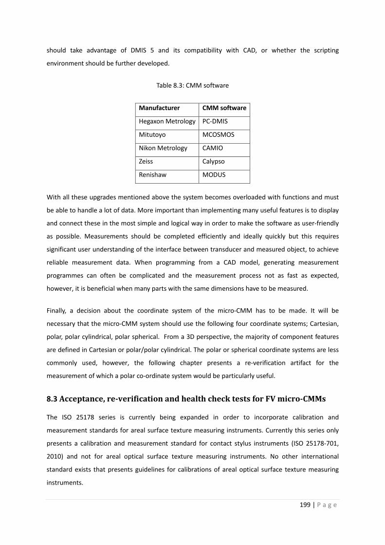
199 | P a g e
should take advantage of DMIS 5 and its compatibility with CAD, or whether the scripting
environment should be further developed.
Table 8.3: CMM software
Manufacturer CMM software
Hegaxon Metrology PC-DMIS
Mitutoyo MCOSMOS
Nikon Metrology CAMIO
Zeiss Calypso
Renishaw MODUS
With all these upgrades mentioned above the system becomes overloaded with functions and must
be able to handle a lot of data. More important than implementing many useful features is to display
and connect these in the most simple and logical way in order to make the software as user-friendly
as possible. Measurements should be completed efficiently and ideally quickly but this requires
significant user understanding of the interface between transducer and measured object, to achieve
reliable measurement data. When programming from a CAD model, generating measurement
programmes can often be complicated and the measurement process not as fast as expected,
however, it is beneficial when many parts with the same dimensions have to be measured.
Finally, a decision about the coordinate system of the micro-CMM has to be made. It will be
necessary that the micro-CMM system should use the following four coordinate systems; Cartesian,
polar, polar cylindrical, polar spherical. From a 3D perspective, the majority of component features
are defined in Cartesian or polar/polar cylindrical. The polar or spherical coordinate systems are less
commonly used, however, the following chapter presents a re-verification artifact for the
measurement of which a polar co-ordinate system would be particularly useful.
8.3 Acceptance, re-verification and health check tests for FV micro-CMMs
The ISO 25178 series is currently being expanded in order to incorporate calibration and
measurement standards for areal surface texture measuring instruments. Currently this series only
presents a calibration and measurement standard for contact stylus instruments (ISO 25178-701,
2010) and not for areal optical surface texture measuring instruments. No other international
standard exists that presents guidelines for calibrations of areal optical surface texture measuring
instruments.

200 | P a g e
Research at the NPL has investigated into calibration procedures of CSI, PSI and ICMs. The work is
published as part of the series “Good practice guides” (Giusca and Leach, 2013(a,b)). Features of the
areal optical surface texture instruments that are suggested to be investigated are as follows:
• measurement noise,
• residual flatness,
• amplification coefficient,
• linearity error,
• perpendicularity of the axes, and
• resolution.
Although all of these characteristics are very important in the context of surface texture
measurements, they are not sufficient to characterise the performance of an instruments in the
context of co-ordinate measurements. An important characteristic of a CMM is its size measurement
accuracy, which should ideally be assessed for the majority of the measurement volume.
Due to the lack of an international calibration and verification standard for areal optical surface
texture measuring instruments, and due to the lack of volumetric size measurement assessments in
guides for calibrating such instruments, this research orientated itself towards the existing
standards, ISO 10360, for assessing the performance of a CMM. The concepts of acceptance, re-
verification and health checks for a CMM have been introduced previously in Chapter 2. Here the
applications of these concepts are presented in more detail.
8.3.1 Acceptance, re-verification and health check tests for CMMs
The ISO 10360 suite of standards has been published by the ISO technical committee ISO/TC 213 as
guidelines for instrument manufacturers and users of CMMs. ISO 10360 was made available to the
public in 1994 and more recently has grown to match the development of newly implemented
techniques in CMMs. The intention was to have an acceptance and re-verification procedures
accepted worldwide by CMM manufacturers. A by-product of the existence of these standards was
better grounds for comparisons between different machine types.
ISO 10360 is a series of standards for a number of different types of CMMs that presents guidelines
to CMM verifications and is entitled “Geometrical Product Specification (GPS) - Acceptance and Re-
verification tests for coordinate measuring machines (CMM)”. Part 2 of ISO 10360 presents an
acceptance and re-verification procedure for a classical tactile CMM (ISO 10360-2, 2009). Parts 3, 4
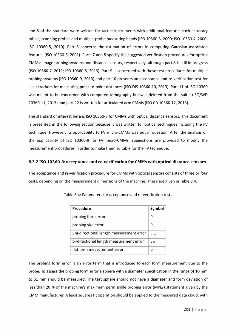
201 | P a g e
and 5 of the standard were written for tactile instruments with additional features such as rotary
tables, scanning probes and multiple-probe measuring heads (ISO 10360-3, 2000; ISO 10360-4, 2000;
ISO 10360-5, 2010). Part 6 concerns the estimation of errors in computing Gaussian associated
features (ISO 10360-6, 2001). Parts 7 and 8 specify the suggested verification procedures for optical
CMMs: image probing systems and distance sensors, respectively, although part 8 is still in progress
(ISO 10360-7, 2011; ISO 10360-8, 2013). Part 9 is concerned with these test procedures for multiple
probing systems (ISO 10360-9, 2013) and part 10 presents an acceptance and re-verification test for
laser trackers for measuring point-to-point distances (ISO DIS 10360-10, 2013). Part 11 of ISO 10360
was meant to be concerned with computed tomography but was deleted from the suite, (ISO/WD
10360-11, 2013) and part 12 is written for articulated arm CMMs (ISO CD 10360-12, 2013).
The standard of interest here is ISO 10360-8 for CMMs with optical distance sensors. This document
is presented in the following section because it was written for optical techniques including the FV
technique. However, its applicability to FV micro-CMMs was put in question. After the analysis on
the applicability of ISO 10360-8 for FV micro-CMMs, suggestions are provided to modify the
measurement procedures in order to make them suitable for the FV technique.
8.3.2 ISO 10360-8: acceptance and re-verification for CMMs with optical distance sensors
The acceptance and re-verification procedure for CMMs with optical sensors consists of three or four
tests, depending on the measurement dimensions of the machine. These are given in Table 8.4.
Table 8.4: Parameters for acceptance and re-verification tests
Procedure Symbol
probing form error PF
probing size error PS
uni-directional length measurement error EUni
bi-directional length measurement error EBi
flat form measurement error ρ
The probing form error is an error term that is introduced to each form measurement due to the
probe. To assess the probing form error a sphere with a diameter specification in the range of 10 mm
to 51 mm should be measured. The test sphere should not have a diameter and form deviation of
less than 20 % of the machine’s maximum permissible probing error (MPEP) statement given by the
CMM manufacturer. A least squares fit operation should be applied to the measured data cloud, with
202 | P a g e
which the thickness of a spherical shell can be calculated that comprises all data points. This set of
measurement data should also be used to determine the probing dispersion value, which indicates
the thickness of a spherical shell that comprises only 95 % of all measured points.
The probing size error is the measurement deviation from the nominal value of the geometric
feature due to the probe. The probing size error assessment as suggested in ISO 10360-8 requires
twenty-five representative points from the data cloud acquired for the probing form error
assessment. These points should be used to obtain the measured sphere diameter by applying the
mathematical least squares method. The CMM’s probing size error is then the difference between
the measured sphere diameter and the calibrated sphere diameter.
Length measurement error gives an indication on the accuracy of the machine's linear scales.
Necessary equipment for the measurement procedure includes five calibrated length bars (or any
other artefact listed in ISO 10360-8 such as ball bars) and a clamp to hold all length bars in place. The
longest length bar is recommended to be at least 66 % of machine's travel in the orientation of the
artefact. The length of all length bars should have approximately equal size difference to the next
bigger length bar. It should be noted that the material should be chosen according to the machine's
technique: ceramics and steel are standards, but a different material may be more appropriate for
different reasons such as colour, reflection factor, optical penetration depth or scattering
characteristics.
The length measurement error assessment requires all five length bars to be measured positioned in
all four body-diagonals, as specified below and illustrated in Figure 8.6, and the user can choose
another three orientations (by default along the X, Y or Z axes). The measurements of all length bars
in each position have to be completed three times, which amounts to 105 measurements in total.
• co-linear with the X axis (default)
• co-linear with the Y axis (default)
• co-linear with the Z axis (default)
• along a volumetric diagonal, XYZ (required)
• along a volumetric diagonal, -XYZ (required)
• along a volumetric diagonal, X-YZ (required)
• along a volumetric diagonal, XY-Z (required)

203 | P a g e
Figure 8.6: Measurement orientations
With the results of the measurements, the instrument’s bi-directional (or uni-directional if bi-
directional measurements are impractical) measurement error, EBi (or EUni), can be isolated by
calculating the difference between the measurement result and the calibrated value of the length
bar. All error values should be plotted with respect to the calibrated length in a graph, which should
also show the tolerance band (MPEE) provided by the manufacturer. The MPEE is commonly quoted
to show the measurement accuracy of the machine.
Artefacts that are suggested to be used for the length measurements are gauge blocks, step gauges,
ball bars or a laser interferometer. An important specification for the first three artefacts is a smooth
surface finish that has a negligible roughness with respect to the CMM’s MPEP or MPEE so that it does
not influence the measurement error but this may be an issue for FV.
8.3.3 Health checks for CMMs with optical distance sensors
ISO 10360 suggests that a re-verification test on any type of CMM is repeated approximately every
six months and that several health checks (or interim checks) are performed regularly and frequently
in between each re-verification. This time scale was suggested because of the re-verification
duration (typically at least one day). Health checks can help a user monitor the instrument
performance and plan the next re-verification date. Health checks can also be performed
spontaneously when the user doubts the instrument performance, i.e. after a collision. In industry,
health check procedures are typically completed within half an hour if the set-up is simple and an
automatic programme is readily available.
ISO 10360 suggests that a health check procedure comprises the probing form and size errors as
suggested for a re-verification test. The length measurement error can be performed with less
measurement data. ISO 10360-8 suggests for example to use only the longest length normally used
for a re-verification test for the length measurements. Suggested artefacts that are suitable for

204 | P a g e
distance sensors and that can be used for health checks are for example a purpose-made test piece,
a ball plate, a grid plate, a ball bar, a line scale and a circular artefact.
8.3.4 ISO 10360-8: potentials and restrictions for FV micro-CMMs
With the prospect of having FV micro-CMMs on the market in the near future, a development of an
acceptance and re-verification standard suitable for FV micro-CMM should ideally be completed as
the micro-CMM is developed. Here, the requirements, methods, and artefacts are discussed for a re-
verification of FV micro-CMMs. Possibilities for a health check procedure are also discussed.
The FV technique is classified as a distance sensor, but the applicability of the ISO 10360-8 to a FV
micro-CMM was questioned here. It may appear straightforward to take a re-verification procedure
for large optical CMMs, scale the artefacts down in size and apply the procedure to an optical FV
micro-CMM; however, this approach may have boundaries, which need to be explored for each of
the tests presented in ISO 10360-8.
8.3.4.1 Measurements for probe form error and probe size error
The test sphere is suggested to have a diameter within the range of 10 mm to 51 mm. An assumption
is that a measurement of a 10 mm test sphere is performed with the sphere’s highest point in the
centre of the objective lens’s FoV. If the objective lenses of a future FV micro-CMM have the same
magnifications and FoV specifications as a IFM G4, the longest line profile over the effective surface
taken diagonally through the FoV covers a maximum of 51 % and 1.2 % of a test sphere’s upper
semicircle using the 2.5× and the 100× objective lenses, respectively. For each objective lens
magnification Table 8.5 specifies the angles, α, associated with the longest arc on the sphere’s
surface measurable with only one FoV, as shown in Figure 8.7. The percentage of the measureable
semicircle is very small especially for the higher magnification objective lenses (above 10×). The lack
of sufficient information over a larger surface area affects the capability of the FV micro-CMM to
measure the test sphere’s form error accurately by means of a sphere fitting procedure, and thus
puts the validity of the re-verification test in question. For this reason, an ISO 10360 standard that is
aimed at FV micro-CMMs should permit the use of test spheres with diameters smaller than 10 mm.

205 | P a g e
Table 8.5: Maximum angle between two points and the sphere centre measurable in one FoV
Lens magnification 2.5× 5× 10× 20× 50× 100×
Angle α (degrees) 91.8 42.1 20.7 10.3 4.1 2.1
% of semicircle with a 10 mm diameter 51.0 23.4 11.5 5.7 2.3 1.2
Figure 8.7: Angle associated with the largest measured arc of the effective surface
Another concern is the specification for the artefact’s surface characteristic: the artefact's surface
roughness should be negligible (lower than 20 %) with respect to the probing form error value.
According to ISO 10360-8, if it is necessary for an artefact to have a surface roughness of 30 nm Ra,
then the CMM manufacturer is not allowed to state a probe form error or probe size error of smaller
than 150 nm. This statement concerns FV instruments because they rely on inherent roughness to
provide contrast in images. For FV micro-CMMs this means that they cannot have an MPEP statement
of better than 150 nm, regardless of the quality of the axes, the optics and the software.
A further issue of measuring spheres to assess the probing form error are sporadic spikes, a form of
measurement noise, that strongly influence the minimum and the maximum deviations from a fitted
sphere to the measurement data. The probing form of the IFM G4 was calculated using all the data
of repeated measurements of a 1.0 mm stainless steel sphere (one FoV) and the IFM G4’s software
V3.5. The probing form was 22.6 μm (± 5.9 μm). This result shows that the probing form error should
be assessed by a residual flatness test. A suitable flatness test procedure for the FV technique is not
documented in ISO 10360-8. The test flat would need to be allowed to feature roughness, and an
averaging procedure as presented in Chapter 5 would need to be specified in the standard.
8.3.4.2 Length measurement error
The length measurement error assessment as suggested in ISO 10360-8 could not be performed on a
FV micro-CMM. The most obvious restriction for a FV micro-CMM is the vertical length measurement
(in the Z orientation). FV instruments typically have short stand-off distances (or working distance).
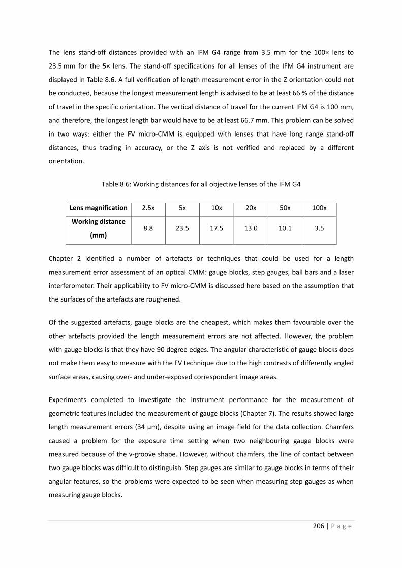
206 | P a g e
The lens stand-off distances provided with an IFM G4 range from 3.5 mm for the 100× lens to
23.5 mm for the 5× lens. The stand-off specifications for all lenses of the IFM G4 instrument are
displayed in Table 8.6. A full verification of length measurement error in the Z orientation could not
be conducted, because the longest measurement length is advised to be at least 66 % of the distance
of travel in the specific orientation. The vertical distance of travel for the current IFM G4 is 100 mm,
and therefore, the longest length bar would have to be at least 66.7 mm. This problem can be solved
in two ways: either the FV micro-CMM is equipped with lenses that have long range stand-off
distances, thus trading in accuracy, or the Z axis is not verified and replaced by a different
orientation.
Table 8.6: Working distances for all objective lenses of the IFM G4
Lens magnification 2.5x 5x 10x 20x 50x 100x
Working distance
(mm) 8.8 23.5 17.5 13.0 10.1 3.5
Chapter 2 identified a number of artefacts or techniques that could be used for a length
measurement error assessment of an optical CMM: gauge blocks, step gauges, ball bars and a laser
interferometer. Their applicability to FV micro-CMM is discussed here based on the assumption that
the surfaces of the artefacts are roughened.
Of the suggested artefacts, gauge blocks are the cheapest, which makes them favourable over the
other artefacts provided the length measurement errors are not affected. However, the problem
with gauge blocks is that they have 90 degree edges. The angular characteristic of gauge blocks does
not make them easy to measure with the FV technique due to the high contrasts of differently angled
surface areas, causing over- and under-exposed correspondent image areas.
Experiments completed to investigate the instrument performance for the measurement of
geometric features included the measurement of gauge blocks (Chapter 7). The results showed large
length measurement errors (34 μm), despite using an image field for the data collection. Chamfers
caused a problem for the exposure time setting when two neighbouring gauge blocks were
measured because of the v-groove shape. However, without chamfers, the line of contact between
two gauge blocks was difficult to distinguish. Step gauges are similar to gauge blocks in terms of their
angular features, so the problems were expected to be seen when measuring step gauges as when
measuring gauge blocks.

207 | P a g e
Ball bars do not have angled surfaces like gauge blocks, so when measuring a sphere with a FV
instrument, the amount of reflected light changes gradually over the curved surface (as shown in
Chapter 7), which facilitates the judgement for light settings. If a sphere's roughness and material
was suitable for FV instruments, a good quality effective surface could be created, of which the
centre could be calculated by a least squares method. The disadvantage of miniature ball-bars are
their impractical handling. So instead of ball-bars, a ball-plate could be used; however, at this point in
time, only one ball plate exists that features a roughness and the dimensions suitable for a FV micro-
CMM (Ehrig, 2009); however, the ball-plate cannot be handled easily in order to allow for an
automated size error measurement procedure. This shows that there is a need for a re-verification
artefact suitable for the FV technique that can be used to automatically re-verify a FV micro-CMM.
8.3.4.3 Health check
ISO 10360 states that a procedure similar to an acceptance and re-verification test but with fewer
measurements can be performed to complete a health check. This gives the user the freedom to test
the instrument with task-specific measurements and it gives the instrument manufacturers the
possibility to suggest procedures for which automation scripts can be offered. The previous section
identified that the use of spheres to define co-ordinate positions is a good method. This means that
an artefact designed for a re-verification procedure would be suitable for a health check as a reduced
number of spheres could be measured to complete the health check procedure.
8.4 Summary
Table 8.7 summarizes how the IFM G4 would need to be improved or changed in order to give it the
capability to function as a micro-CMM. It was found that the general structure of the IFM G4 is
suitable for a micro-CMM. The XY stage encoders and accuracy would have to be improved so that
the positional accuracy could be below 250 nm. Measurements of the IFM G4’s measurement noise
and residual flatness showed to be within or close to the target values for a FV micro-CMM. With
regard to the instrument software, changes would have to be made, in order to incorporate a CAD
kernel and the necessary software to allow for geometric measurements and datum alignment. An
acceptance and re-verification procedure and a health check do not exist for the IFM G4 that could
demonstrate the instrument performance in terms of geometric measurements.

208 | P a g e
Table 8.7: Specification of the IFM G4 and a FV micro-CMM
Aspect IFM G4 FV micro-CMM
Structure Column-bridge with XY stage Column-bridge with XY stage
XY stage encoders Unknown Optical encoders
XY stage accuracy Up to 16.87 μm Below 250 nm
Rotary axis Existing feature Should be part of micro-CMM
Objective lenses 2.5× to 100× 2.5× to 100×
Measurement noise Up to 40 nm for 10× Below 50 nm
Flatness error Up to 7.3 nm for 10× Below 5 nm
Vibration isolation system Passive Passive
CAD kernel Not existing in software V3.5 Must be integrated
CAD software Not existing in software V3.5 Must be integrated
Object weight Limited to 35 kg Limit is dependent on XY
stage specifications
Areal size of features to be
measured
100 mm × 100 mm 100 mm × 100 mm
Datum alignment Not existing in software V3.5 Must be integrated
Acceptance and re-verification ISO 25178 Must be specified
Health check Chess-board artefact and step
height
Must be specified

209 | P a g e
Chapter 9: Novel re-verification artefact
9.1 Introduction
The aim of this chapter is to present the development of a novel acceptance and re-verification
artefact that has the potential to be used for the completion of an acceptance test, a re-verification
test and a health check test of a FV micro-CMM. For simplicity, the acceptance and re-verification
artefact will here be referred to as the re-verification artefact. Especially relevant for this chapter are
the two previous chapters, where the measurement results of simple geometric features (angled
surfaces, gauge blocks and spheres) and where an acceptance and re-verification procedure for FV
micro-CMMs were presented.
The literature review (Chapter 2) presented a number of re-verification artefacts, none of which
were found to be suitable to test a FV micro-CMM primarily because the surfaces of these re-
verification artefacts were too reflective. Of course these specular surfaces could be modified to
have a roughness, but then it was found that their size or shape was not compatible with the object
specification for typical FV instruments (size < 75 mm × 75 mm; the shape has to be such that it
ensures no collision with the lenses during the measurement process). Some existing artefacts
required measurement procedures that could not be met by an areal optical instrument, such as the
measurement around the equator of a sphere. These were the reasons for the need of a novel re-
verification artefact that can serve for an acceptance and a re-verification of a FV instrument. Ideally
the artefact should be suitable for a health check but this was regarded as a secondary issue.
This chapter is organised so that the product design specification of the re-verification artefact is
given first, followed by a description of each artefact design that led to the final artefact, Artefact
Fritz. This final artefact was then calibrated with a CMM and measured with the IFM G4, of which
the results presented, compared and discussed here. The chapter closes with a comparison of the
initial product design specification and the final design, and the performance of the final artefact in
the context of relevant standards.
9.2 Artefact specification
The development of a design for a novel artefact for acceptance, re-verification and possibly also
health check procedures should begin with a detailed specification of factors that potentially
influence the design. These influences may come from the customer, the market, the instrument
210 | P a g e
manufacturer, or the artefact manufacturer. The British Standard document entitled ‘Product
Specification’ (BS 7373-2, 2001) was used as guidance.
To achieve market acceptability of a new FV micro-CMM it is necessary to have a re-verification
artefact readily available to be sold together with the micro-CMM. Discussion with FV instrument
manufacturers (and observation of other artefacts) has led here to the artefact specifications
designed to suit the instrument needs of the IFM G4.
Customers:
• Anyone (or company) who owns a FV micro-CMM
• Anyone (or company) that offers re-verification services
Customer needs:
• The artefact should be an easily manageable object, in terms of handling and weight
(< 800 g).
• The artefact should not be larger than 75 mm × 75 mm × 75 mm.
• The artefact material’s thermal expansion coefficient should be less than 20 × 10-6 / K.
• The artefact design should appear to be simple (in terms of geometric shape).
• Its functionality should be intuitive by its design.
• The re-verification procedure performed with this artefact should be as similar as possible to
the size error measurement procedure presented in ISO 10360-8.
• The measurement uncertainty of the artefact calibration should be better than 50 nm.
• The measurement accuracy of the artefact calibration should be better than 100 nm.
• The artefact should have a lifetime of approximately ten years.
• The artefact should be specific for FV micro-CMMs.
• The artefact should have a colour, reflection factor, optical penetration depth and scattering
characteristics that allow for an easy measurement set-up.
• The artefact should be offered with the necessary fixture devices.
• The artefact should be traceable to the metre at a national institute such as the NPL (UK) or
the PTB (Germany).

211 | P a g e
The market:
• The artefact should be specific for FV micro-CMMs but should have the potential to expand
into the markets for any other types of areal micro-CMM.
• The artefact could be brought to customers through FV micro-CMM manufacturers or
National Measurement Institutes, such as the UK NPL, that are otherwise also concerned
with certification of micro-CMMs, or the artefact manufacturer themselves.
• There should be no difference in the design of the artefact regardless of where the artefact
was sold to.
• Transportation of the artefact should be straightforward and easily manageable.
• Transport protection should be simple, and it should ideally present the artefact to the user.
Competitor information:
• At this point in time (as a function of detailed literature survey), the author believes that
there are no competitors for a FV specific re-verification artefact.
Performance characterisation and definition:
• The artefact should have at least one set of five different lengths in order to establish the
size measurement error of a FV micro-CMM conforming to ISO 10360-8.
• Defined lengths must be measurable in at least seven different orientations, of which four
must be body-diagonals.
• The re-verification process should be as short as possible, no longer than one day.
• A health check procedure using the artefact should be able to be performed within
approximately 30 minutes.
• All measurement points must be well defined.
• The measurement points should not be easily influenced by temperature, humidity or noise.
• The artefact should have a random roughness that is the same at all measurement locations
and approximately 30 nm Ra.
• The number of measurements should be kept to a minimum but conform to ISO 10360-8.
• A re-verification of the vertical axis (without moving the XY stage) can only be completed
with small step heights.
• The artefact’s manufacturing should be uncomplicated.
• The product should be robust to vibrations and handling.

212 | P a g e
• The artefact should be easy to measure with a low risk of collision of the objective lens and
the object.
• The artefact should be easy to clean.
• The artefact should be heavy enough not to move when being measured.
The ISO 10360 acceptance and re-verification procedure has been an international standard since
1994 and is today well-established in field of co-ordinate metrology. A re-verification procedure for a
FV micro-CMM would be best accepted, if it was closely related to existing CMM re-verification
procedures, because most CMM users are already familiar with the ISO 10360 re-verification
procedures. As previously identified (Chapter 7) the ISO 10360 is a collection of several parts (of
which the first part is introductory) that each concern a different type of CMM. In all parts of the ISO
10360 document, size measurement error is suggested to be established by measuring five different
lengths in seven orientations. ISO 10360-8 addresses optical CMMs and consequently the re-
verification procedure suggested was regarded as an appropriate process for a FV micro-CMM if the
lengths of the length-defining artefact were adapted to the measuring volume of the FV micro-CMM.
The question here is whether to make an artefact that requires repositioning when re-verifying
different measurement directions or whether the artefact should be made with additional
measurement points to allow for an uninterrupted size measurement error procedure. The
advantage of the prior is a less complicated calibration procedure of the re-verification artefact and
the advantage of the latter is a less complicated re-verification procedure that can be automated
because the artefact would not have to be orientated differently during the re-verification
procedure.
The experiment with gauge block measurements presented in Chapter 7 demonstrated that results
of distance measurements using sharp edges were inaccurate and imprecise. The conclusion from
that set of measurement results was to use curved surfaces that can be measured well with the FV
technique. A single measurement point on a curved surface is difficult to define, but simple
geometric shapes such as a cylinder or a sphere have well-defined points and lines, i.e. cylinder axis
and sphere centre, the positions of which could be calculated by surface measurements and
geometric shape fitting. Obviously the measurement of such geometric shapes is affected by
measurement error of the FV micro-CMM.
The advantages that spheres have over other shapes are simplicity and a singular point that defines
a sphere's position. Additionally, a sphere's centre is not strongly affected by temperature change.

213 | P a g e
For instance, if a sphere was floating in mid-air, and heated, its material would expand in all
directions, leaving the coordinates of the sphere's centre unchanged. However, it is impossible (or
very impractical) to place a sphere statically in mid-air in the measuring volume of the FV micro-
CMM, and therefore, a sphere has to be located on a substrate that can be handled easily.
Consequently, a temperature change can influence the height of each individual sphere's centre, but
this phenomenon is negligible for a re-verification procedure under the condition that all spheres are
affected in the same manner. For example if a 1 mm diameter sphere of stainless steel (Grade 316)
with a thermal expansion coefficient of 16 × 10 / K was exposed to a temperature change of 1 K then
the sphere diameter would expand by 16 nm. This change in diameter is very small with respect to
the uncertainty budget of the re-verification artefact. This condition requires the spheres to be of
the same material and the same size, i.e. a repeatable manufacturing process of the spheres. The
restriction of size does not apply to good quality hemispheres because the centre points are ideally
in contact with the substrate. There is an advantage to having a substrate that the spheres are
bound to: the substrate can have a larger thermal mass compared to the size of the spheres and
thus make the spheres less affected by thermal fluctuations.
Some of the existing re-verification artefacts, such as the ETH ball reference plate (see
Section 2.4.4.1) used sphere centres to define measuring points. These re-verification artefacts
showed good uncertainties of the sphere positions (U = 2.1 μm (k = 2), Liebrich et al., 1009). Very
high quality spheres or hemispheres with small form errors or surface roughness have been used for
these re-verification artefacts. Any form error is a source of uncertainty of the sphere measurement,
especially when only a few points are used for sphere fitting.
For the case of FV micro-CMMs the surface of the sphere must have a random roughness that has a
minimal effect on the form of the sphere or an inherently contrasted surface. There are two
possibilities to produce spheres with roughness: either a sphere is not lapped to meet the usual
standards used for re-verification artefact spheres, or the roughness is applied to a high quality (e.g.
grade 3) sphere by particle blasting or chemical etching. The disadvantage of the prior method is a
larger form error, and the disadvantage of the latter is the variability of size between spheres and
possibly an introduction of form error to each sphere.
In general, the smaller the number of measurement scans (measurement with one FoV), the shorter
the re-verification duration. However, the number of measurement scans (or FoV per measurand) is
dictated by the accuracy of the measurement. For example, in the case of spheres and hemispheres,

214 | P a g e
their dimensions (diameters) can be chosen so that a good balance between measurement time and
the necessary number to accurately establish the sphere's centre.
It is essential that all spheres have the same roughness. PTB has completed work that investigated
the instrument response of roughness measurements on sloped surfaces by using spheres with
different roughness. The conclusion was that the rougher the surface is, the larger the angle is at
which the FV instrument can detect the surface (Ehrig, 2009). This finding was strengthened by the
results of radius measurements of spheres (presented in Chapter 7) comparing different materials
and quality grading. The grade 100, 1.0 mm diameter stainless steel spheres could be measured
better (radius measurement deviation of 1 μm) than the grade 3 zirconia spheres of the same size
(radius measurement deviation of 7 μm).
The last issue is the re-verification of the vertical axis. In ISO 10360, it is stated that the vertical axis
should be re-verified if no alternative is suggested by the instrument user. A FV instrument cannot
measure a step height of more than a few millimetres, depending on the stand-off distance of the
objective lens being used. On the IFM G4 the largest stand-off distance is 23.5 mm for the 5×
objective. This distance does not cover 66 % of the maximum vertical movement (100 mm) that the
instrument is capable of and, therefore, a step height artefact is not suitable to re-verify the Z axis. A
difference in the Z height of two spheres for example could be measured however, a lateral
movement is necessary for the measurement, which could affect the re-verification of the Z axis.
9.3 First concept of a re-verification artefact for FV micro-CMMs
One of the key novelty aspects of this thesis lies with the development of a re-verification artefact.
Here, the development will be presented, including all erroneous directions that were attempted.
The first concept was to use existing reference specimens that could be used to measure lengths,
arranged in particular orientations for a re-verification of FV micro-CMMs. A potential source for
such specimens for length measurements was Rubert & Co Ltd (Rubert, 2013), a manufacturer of
high quality surface roughness reference specimens, who has in the past delivered to the UK NPL. A
part of the roughness reference range offered by Rubert is shown in Table 9.1. All of these listed
specimens are sinusoidal in nature, potentially suitable for distance measurements. The column in
Table 9.1 marked with ‘ISO type’ is a classification for reference specimen documented in ISO 5436-1
(ISO 5436-1, 2000). Specimens of type ‘B’ were designed for the verification of stylus tip conditions
and type ‘C’ are spacing measurement standards with regular-profiles for checking the performance
of stylus instrument and parameter evaluation.

215 | P a g e
Table 9.1: Sinusoidal roughness references (Rubert, 2013)
Item
number
ISO
Type
Parameter
values
Roughness
values Shape Profile
525 C RSm = 135 µm
Pt = 19 µm Ra = 6.25 µm sine wave
526 C RSm = 100 µm
Pt = 10 µm Ra = 3.15 µm sine wave
527 C RSm = 100 µm
Pt = 10 µm Ra = 3.0 µm sine wave
528 C RSm = 50 µm
Pt = 1.5 µm Ra = 0.5 µm sine wave
529 C RSm = 10 µm
Pt = 0.3 µm Ra = 0.1 µm sine wave
530 C RSm = 100 µm
Pt = 3.0 µm Ra = 1 µm sine wave
531 C RSm = 100 µm
Pt = 1.0 µm Ra = 0.3 µm sine wave
542 B, C RSm = 8 µm
Pt = 0.2 µm Ra = 0.06 µm sine wave
543 B, C RSm = 2.5 µm
Pt = 0.12 µm Ra = 0.04 µm sine wave
Alicona has in the past obtained roughness references from Rubert, roughened them by particle
blasting, and demonstrated their suitability for FV measurements (Danzl, 2011). Figure 9.1 shows an
image of an effective surface of a roughness specimen (item number 528, with an RSm of 135 µm, a
Pt of 1.5 µm and an Ra of 0.5 µm) obtained by the IFM G4. In a previous section (Chapter 6) on high
aspect ratio measurements with the FV technique, it was shown that a sinusoidal roughened
roughness reference specimen can be measured at angles up to 40 degrees.
Figure 9.1: IFM G4 measurement of a sinusoidal roughness artefact (Alicona, 2009)

216 | P a g e
The separations between peaks of this particular specimen are small (RSm = 135 μm) compared to
the length measured, providing seven peaks within 1.0 mm of horizontal distance. The distance
between any two peaks should be multiples of 135 μm. The disadvantage of this specimen is that it
becomes impractical when measuring for example a length of 29.97 mm: a time-consuming line scan
would have to be completed and then 222 peaks would have be counted to ensure that the correct
peak was being used for the length measurement.
The first concept of a re-verification artefact can be seen in sketched form in Figure 9.2. The
roughness reference specimens would have been inserted into a substrate so that each of these
specimens would be orientated to conform the measurement orientations suggested in ISO 10360-2
(ISO 10360-2, 2001) before the new version of the document was published in 2009. With this
artefact, the re-verification process could be carried out without interruptions (i.e. re-orientation of
the artefact). The measurement orientations shown in Figure 9.2 are X, Y, XY, XZ, YZ and XYZ.
Because this concept was based on an outdated version of ISO 10360-2 from 2001 the development
of the artefact never reached the detailed design stage. According to the latest editions of ISO
10360 parts 2 and 8, only the four body-diagonals, of which only one is present in the drawing, are
obligatory. The six orientations suggested in the sketch, would not bring the re-verification
procedure of a FV micro-CMM close to that of traditional CMMs. This artefact was a stepping stone
in the development of the final re-verification artefact.
To conclude, the first concept was discarded because the measurement orientations did not meet
the criteria of the latest edition of the ISO 10360-2 standard. Additionally to the inadequate
measurement orientations, the inserted calibration artefacts, which would have been used for the
length measurements, were impractical as they would have required line scans in order to find the
correct peak for the length measurement.
Figure 9.2: First concept for a re-verification artefact

217 | P a g e
9.4 Artefact number two
The second idea was developed whilst ISO 10360-2 was in the process of being updated and before
the draft version of ISO 10360-8 was circulated and became available within the research project.
The development focused on the method of distance measurement. By setting up four
measurement points on a virtual straight line at varying distances to each other six different lengths
can be measured, as shown in Figure 9.3. Note that this setup required point measurements, instead
of line scans, and it required the minimum number of measurements (four) in order to measure at
least five lengths. The three bi- and multi-directional orientations also present in the previous sketch
were used here (XZ, XYZ and YZ). Because of the IFM G4’s cubic measuring volume (with side lengths
of 100 mm) the angle of the bi-directional orientation should be at 45 degrees; however, the body-
diagonal would only have to have an angle of 35.27 degrees but was kept at 45 degrees for
simplicity.
Figure 9.3: Six axial distances (a-f) between four non-equispaced spheres
By choosing the sphere separations carefully, the criteria given in the ISO 10360-2 standard can be
fulfilled: along the X axis, the centres were at 6.0 mm, 11.0 mm and 15.0 mm from the centre of the
sphere. The other two lines of measurement were rotationally symmetric to the first. The angle of
the virtual lines was kept at 45 degrees, so the height of the spheres at 6.0 mm distance was 6.0 mm
and respectively for the other elevated spheres. The six distances that could be measured between
spheres aligned in one orientation (with reference to Figure 9.3) were 5.66 mm (c), 7.07 mm (b),
8.48 mm (a), 12.73 mm (e), 15.55 mm (d), and 21.21 mm (f). This is also shown in Figure 9.4. The first
three values are the closest in this set of lengths, so if the second length was ignored, that would
leave five approximately evenly distributed values within the range from the smallest to largest
distance.
It should be noted that at the time when this re-verification artefact was designed, the measuring
volume specification of the FV micro-CMM was unknown. The maximum length chosen did not cover
66 % of the body diagonal of the IFM G4's measuring volume; however, this design could be scaled
to suit any cubic volume.
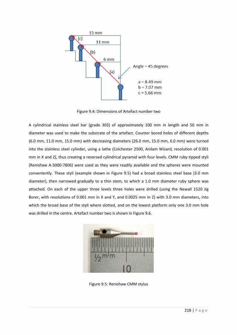
218 | P a g e
Figure 9.4: Dimensions of Artefact number two
A cylindrical stainless steel bar (grade 303) of approximately 100 mm in length and 50 mm in
diameter was used to make the substrate of the artefact. Counter bored holes of different depths
(6.0 mm, 11.0 mm, 15.0 mm) with decreasing diameters (26.0 mm, 15.0 mm, 6.0 mm) were turned
into the stainless steel cylinder, using a lathe (Colchester 2500, Anilam Wizard, resolution of 0.001
mm in X and Z), thus creating a reversed cylindrical pyramid with four levels. CMM ruby tipped styli
(Renishaw A-5000-7806) were used as they were readily available and the spheres were mounted
conveniently. These styli (example shown in Figure 9.5) had a broad stainless steel base (3.0 mm
diameter), then narrowed gradually to a thin stem, to which a 1.0 mm diameter ruby sphere was
attached. On each of the upper three levels three holes were drilled (using the Newall 1520 Jig
Borer, with resolutions of 0.001 mm in X and Y, and 0.0025 mm in Z) with 3.0 mm diameters, into
which the broad base of the styli where slotted, and on the lowest platform only one 3.0 mm hole
was drilled in the centre. Artefact number two is shown in Figure 9.6.
Figure 9.5: Renishaw CMM stylus

219 | P a g e
Figure 9.6: Artefact number two
The artefact was tested for accessibility of the spheres using the IFM G4 50× magnification lens.
Although none of the spheres were measured with the FV technique, all of the spheres were
observed in focus within the instrument software. At no position did the 50× magnification lens
collide with any part of the re-verification artefact. This was a positive outcome of the testing but
the preliminary testing identified that the design of the inversed cylindrical artefact was not ideal
because the objective was relatively close to parts of the artefacts when lower spheres (such as the
sphere at the origin) were probed, and the artefact was difficult to clean (the bottom counterbore is
a dirt trap). With the objective lens being closed in by the artefact when measuring the lowest
sphere, this measurement procedure does not convey confidence in the user that it is a safe
procedure.
The reflective and translucent nature of the ruby spheres led to the parallel investigation
concerning: what material was most suited for FV measurements; what surface roughness was most
suitable; and how image field measurements differed from single FoV measurements. In brief, the
conclusion was to use 1.0 mm diameter grade 100 stainless steel spheres for any subsequent re-
verification artefacts, because their measurements were repeatable and the spheres were cheap, as
identified in Chapter 7.
9.5 Artefact design: mission Fritz
Development of the artefact design required detailed CAD drawings and models, as shown in
Figure 9.7. This model shows the third generation artefact, which for simplicity reason will be
referred to as Artefact Hans. Artefact Hans was rotationally symmetric in nature, designed as a non-
inversed cylindrical pyramid (extending from the concept previously detailed) because this would
increase the user’s confidence that the lens does not collide with the re-verification artefact and it is

220 | P a g e
easier to clean. The substrate was made of stainless steel 303. On the top level was placed one
1.0 mm stainless steel sphere. All three lower levels were platforms for eight 1.0 mm stainless steel
spheres equally spaced on pitch circle diameters (PCDs). The spheres on different levels were aligned
similarly to the concept of artefact number two (Section 9.4), and likewise the virtual lines
connecting four spheres were at 45 degrees. Note that Renishaw do not supply stainless steel sphere
styli, so individual stainless steel spheres (grade 100) were used. The tolerance on each of the
dimensional specifications was ± 20 μm.
Figure 9.7: Drawing of Artefact Hans
The manufacture of Artefact Hans was completed with the machines used for the previous artefact:
a numerically controlled turning centre was used to make the step heights (Colchester 2500, Anilam
Wizard, resolution of 0.001 mm). For the location of the spheres, holes were drilled using a Newall
1520 (Jig Borer, Anilam Wizard, with resolutions of 0.001 mm in X and Y axes, and 0.0025 mm in Z
axis) with a 90 degrees point spot carbide drill that had a drill head diameter of 4.0 mm. Into the
holes Cyanoacrylate adhesive was deposited by pointing the nozzle of the adhesive bottle directly to
the hole. Excess adhesive was wiped off before a sphere was carefully placed in the shallow hole
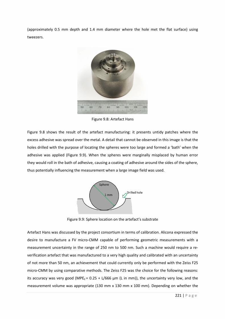
221 | P a g e
(approximately 0.5 mm depth and 1.4 mm diameter where the hole met the flat surface) using
tweezers.
Figure 9.8: Artefact Hans
Figure 9.8 shows the result of the artefact manufacturing: it presents untidy patches where the
excess adhesive was spread over the metal. A detail that cannot be observed in this image is that the
holes drilled with the purpose of locating the spheres were too large and formed a ‘bath’ when the
adhesive was applied (Figure 9.9). When the spheres were marginally misplaced by human error
they would roll in the bath of adhesive, causing a coating of adhesive around the sides of the sphere,
thus potentially influencing the measurement when a large image field was used.
Figure 9.9: Sphere location on the artefact’s substrate
Artefact Hans was discussed by the project consortium in terms of calibration. Alicona expressed the
desire to manufacture a FV micro-CMM capable of performing geometric measurements with a
measurement uncertainty in the range of 250 nm to 500 nm. Such a machine would require a re-
verification artefact that was manufactured to a very high quality and calibrated with an uncertainty
of not more than 50 nm, an achievement that could currently only be performed with the Zeiss F25
micro-CMM by using comparative methods. The Zeiss F25 was the choice for the following reasons:
its accuracy was very good (MPEE = 0.25 + L/666 μm (L in mm)), the uncertainty very low, and the
measurement volume was appropriate (130 mm x 130 mm x 100 mm). Depending on whether the

222 | P a g e
Zeiss F25 was used at the NPL or at the PTB (these are the two most likely options due to existing
connections) either comparative methods would be used or a reversal method that would minimise
the measurement uncertainty (Trapet, 1991), the latter producing a more accurate calibration
statement. A problem that poses for both methods was the large height variation of the artefact.
Whilst this was desirable for the FV micro-CMM, it was less desirable for the calibration chain and
the use of a Zeiss F25.
Three main changes were investigated to the artefact design of Artefact Hans, which led to Artefact
Fritz. Firstly, the angles of the virtual straight lines with respect to the horizontal were lowered from
45 degrees to 36 degrees (the angle of a body diagonal of a cubic volume), maintaining the X and Y
co-ordinates of the most outer spheres (they were kept on a 30 mm PCD around the origin). This
change was performed to conform to ISO 10360-8 that suggests four of the measurement
orientations to be parallel to body diagonals. Unfortunately, one value was calculated wrong and
this error resulted in a bent virtual line. This does not, however, influence the principle that was
aimed to be demonstrated here. In Figure 9.3 the value 2.54 mm should be 3.26 mm.
Secondly, the horizontally projected separations of the spheres were changed so that the smallest
PCD (defined by sphere centres) radius was 4.5 mm, followed by 9.0 mm and 15.0 mm. All
dimensions of the artefact are shown in Figures 9.10 and 9.11. This set up still allowed the
measurement of five different distances along the (bent) virtual line through the sphere centres:
5.167 mm (a), 6.014 mm (b), and 7.417 mm (c) between neighbouring spheres, and 11.119 mm (d),
13.415 mm, (e) and 18.536 (f) for the other combinations, with respect to Figure 9.3. The difference
between the two smallest separations was only 0.847 mm, which may not be ideal for a re-
verification that requires an even spread of measurable lengths over a given range. Table 9.2
presents the CAD model generated X, Y and Z co-ordinates of all sphere centres. The tolerance on
each of the dimensional specifications was ± 20 μm.
Figure9.10: Dimensions of Artefact Fritz

223 | P a g e
Figure 9.11: Drawing of Artefact Fritz

224 | P a g e
Table 9.2: CAD generated XYZ co-coordinates of all 25 spheres
Sphere no. X (mm) Y (mm) Z (mm)
1 0.000 0.000 0.000
2 4.500 0.000 -2.543
3 9.000 0.000 -6.539
4 15.000 0.000 -10.898
5 0.000 4.500 -2.543
6 0.000 9.000 -6.539
7 0.000 15.000 -10.898
8 -4.500 0.000 -2.543
9 -9.000 0.000 -6.539
10 -15.000 0.000 -10.898
11 0.000 -4.500 -2.543
12 0.000 -9.000 -6.539
13 0.000 -15.000 -10.898
14 3.181 3.181 -2.543
15 6.364 6.364 -6.539
16 10.607 10.607 -10.898
17 -3.181 3.181 -2.543
18 -6.364 6.364 -6.539
19 -10.607 10.607 -10.898
20 -3.181 -3.181 -2.543
21 -6.364 -6.364 -6.539
22 -10.607 -10.607 -10.898
23 3.181 -3.181 -2.543
24 6.364 -6.364 -6.539
25 10.607 -10.607 -10.898
Finally, the method of locating spheres was revised: holes with 0.5 mm diameter would ensure that
the sphere would be located largely above the surface (as shown in Figure 9.12). The adhesive would
be placed with more control: a small pool of adhesive was created, and a metal pin was used to
transfer small amounts of adhesive to the locations of the holes before placing the stainless steel
spheres over these.

225 | P a g e
Figure 9.12: Revised design for sphere location
Figure 9.13 presents the final re-verification artefact, Artefact Fritz. It was noticeable that the
revised method of applying the cyanoacrylate adhesive and locating the spheres was successful. The
artefact was inspected under a Leica microscope (MZ 12(5)) for any patches of adhesive on the top
half of the spheres and none were found, which indicated good assembly of the artefact.
Figure 9.13: Artefact Fritz
With regard to a calibration of the re-verification artefact, it could be completed by repeatedly
measuring the spheres at different rotation angles in order to minimise the measurement
uncertainty of the Zeiss F25 measurements. In the following is an outline of a possible calibration
procedure:
1. Clean the artefact;
2. Place the artefact in the centre of the micro-CMM’s measuring volume
3. Measure all 25 spheres three times (first set of data);
4. Rotate the artefact by 90 degrees;
5. Re-define the artefact’s co-ordinate volume;
6. Re-measure all spheres three times (second set of data);
7. Rotate the artefact by 90 degrees;

226 | P a g e
8. Re-define the artefact’s co-ordinate volume;
9. Re-measure all spheres three times (third set of data);
10. Rotate the artefact by 90 degrees;
11. Re-define the artefact’s co-ordinate volume;
12. Re-measure all spheres three times (fourth set of data);
13. From the four sets of data calculate the mean co-ordinate values for the positions of each
sphere;
14. The uncertainty budget is defined by the largest standard deviation of all four sets of data.
The research presented here does not comprise a calibration procedure of the re-verification
artefact, Artefact Fritz, using a micro-CMM. An investigation of a calibration procedure for Artefact
Fritz is part of the work that would advance this research.
9.6 Size error measurements using Artefact Fritz
The intention of this set of measurements was to demonstrate that Artefact Fritz was developed to
suit a FV micro-CMM. The previous section presented the development of Artefact Fritz and a
discussion about its design, material, manufacturing method, and method of calibration. This section
should show if the design serves its functional purpose. Before any artefact can be used for a re-
verification of a CMM it must be calibrated by another technique that is able to carry out the
dimensional measurements with an uncertainty of less than 10 % of the CMM that is to be re-
verified. This implies that a re-verification artefact only then has value, when the length defining
features have an uncertainty budget. Here, Artefact Fritz was calibrated with the Metris Ultra CMM
in order to provide comparative positional co-ordinates of the sphere centres.
9.6.1 Method
The calibration was performed on the Metris Ultra CMM that was situated in the same laboratory,
and, therefore, was exposed to the same temperature and humidity conditions as all previous
experiments. For the measurement of Artefact Fritz, a Renishaw contact kinematic touch trigger
probe (TP 20) was used with a probe sphere diameter of 0.3 mm. The software of the Metris Ultra
was Camio V6.1 and the programming language was DMIS V5.2. The machine's uncertainty
specification when using the TP20 probe was 3 μm for the whole measuring volume, however, for a
measurement distance of 15 mm an uncertainty of 1 μm could be expected.

227 | P a g e
A datum alignment was performed before the sphere measurements were carried out, aligning the X
and Y axes of the measurement volume with those of the artefact and setting the origin to the
centre of the top sphere. Each of the eight sets of three spheres aligned radially from the origin was
measured so that the sphere closest to the origin was measured first and the most outer sphere of
the set last (see Figure 9.14). The procedure to measure all 25 spheres was performed three times
repeatedly. Each measurement was conducted by contacting the sphere at five points, of which four
were evenly distributed around each sphere's equator and one on the top of each sphere. The
timescale of these measurements was much shorter than the measurements with the IFM G4, and
took approximately one hour in total.
Figure 9.14: Measurement orientations
Artefact Fritz was placed in the centre of the XY stage. The process of measuring all 25 spheres using
only one FoV for each measurement was performed three times. The data collection of each sphere
(including re-locating the sensor) took approximately three to four minutes (total = 4.5 hours). To all
measurements (or effective surfaces) a virtual sphere was fitted using the software provided with
the IFM G4, and the X, Y and Z co-ordinates of each sphere were recorded. Because the IFM G4 does
not have software that supports co-ordinate measurements, each set of 25 sphere centres had to be
translated (by subtracting the coordinate values of sphere 1 from all other sphere coordinates) and
rotated (by finding the angle, at which the deviation to the artefact design coordinate values were
smallest) in a post processing procedure, so that the centre of the top sphere was at the origin for
each of the three repeats. With three co-ordinates of the centre of each sphere, a mean position for
each sphere could be calculated and used for comparisons.
9.6.2 Results
9.6.2.1 Calibration of Artefact Fritz
The Metris Ultra CMM was the most accurate CMM available at Loughborough University and,
therefore, used for calibration of Artefact Fritz. This CMM was last re-verified in June 2013, using

228 | P a g e
calibrated length bars that were traceable to the metre at the NPL. The disadvantage to using the
large CMM was the contact force (YX: 0.08 N, Z: 0.75 N) applied to the artefact. As a result of
contacting and of the insufficient amount of adhesive used for bonding the spheres in place, two
spheres were knocked off the artefact during the measurement process. It was found that sufficient
data was available to prove the principles without replacing these spheres. The data presented in
Figure 9.15 is the mean of three absolute CMM measurement deviations from the nominal values
given in the CAD model specifications of the artefact. The magnitude of each mean deviation is
represented in Figure 9.15 by the bubbles’ width with a magnification factor of 20, to make them
more visible on the axes’ millimetre scale. Because the CMM uncertainty is known by the MPEE
formula, but not the manufacturing uncertainty, the measured deviations from the nominal design
values measured with the CMM are (realistically) the errors caused by the manufacturing process.
Two significant deviations, 152 μm and 98 μm, from the target co-ordinates were observed; all other
deviations were below 70 μm from the target co-ordinates. The smallest deviations were seen for
the measurements in the Y(-Z) and XY(-Z) orientations.
Figure 9.15: Deviation of sphere centres from values of the artefact specifications
152.16 13.36
7.30
11.70
25.60
57.96 50.59 69.29
41.83
26.38
6.23
21.11
7.79
28.80
29.06
98.10
25.19
63.21
25.60
45.34
27.46
26.32
-20
-15
-10
-5
0
5
10
15
20
-20 -15 -10 -5 0 5 10 15 20
X axis / mm
Y axis / mm
CMM measurement / micrometres

229 | P a g e
It is difficult to present all necessary information in one graph and maintain a clear view over the
results; therefore, a separate graph (Figure 9.16) presents the standard deviations of the CMM mean
positional measurement results. The mean of all standard deviations was 409 nm: only three
standard deviations were below 200 nm and the largest standard deviation was 616 nm. No
relationship was seen between the sphere’s distance from the origin and the magnitude of the
measurement’s standard deviation.
Figure 9.16: One standard deviation of the CMM measurements
9.6.2.2 Application of Artefact Fritz to the IFM G4
The co-ordinates of the sphere centres of Artefact Fritz were measured with the IFM G4 instrument
with two intentions: to investigate the accuracy of the sphere position measurements and to
investigate the applicability of Artefact Fritz for the execution of ISO 10360-8.
0.334 0.190
0.136
0.154
0.384
0.386 0.432 0.398
0.453
0.535
0.447
0.506
0.551
0.434
0.616
0.526
0.530
0.557
0.591
0.463
0.355
0.438
-20
-15
-10
-5
0
5
10
15
20
-20 -15 -10 -5 0 5 10 15 20
X axis / mm
Y axis / mm
Standard deviation of CMM measurements / micrometres

230 | P a g e
Sphere position measurements with the IFM G4
The co-ordinate measurement results of the IFM G4 cannot be presented as measurement errors
against the values specified in the CAD model design, because the manufacturing uncertainty is not
known and the uncertainty of IFM G4 co-ordinate measurements is not known, however, previous
investigations have shown that sphere measurement errors and positional errors (16.87 μm) can be
expected (Chapter 7 and Section 8.2.2). The manufacturing uncertainty can be roughly estimated by
summing in quadrature the estimated uncertainty introduced in each manufacturing process step,
which included the lathe, the drill, and the bonding of the spheres to the substrate. The difference
between the IFM G4’s co-ordinate measurements from the intended positions would not provide
any sensible information. However, the standard deviations of the IFM G4 measurements provide
meaningful information and are mapped in a separate bubble chart (Figure 9.17). The widths of the
bubbles represent one standard deviation, up-scaled by a factor of ten to make them visible.
With the exceptions of the measurements along the Y(-Z) axis, the measurements in all other
orientations show a relationship between the sphere distance from the origin and measurement
standard deviation: the further the sphere is positioned from the origin, the larger is the
measurement deviation. Excluding the results obtained in the Y(-Z) orientation again, the range of
measurement standard deviation magnitudes for the smallest circle of spheres was from 2 μm to 30
μm, for the second circle the range was from 15 μm to 39 μm and for the largest circle it ranged
from 38 μm to 74 μm. The general increase of standard deviation from the smallest to the largest
circle was almost by a factor 10. The two largest standard deviations were associated with the
measurements in the X(-Z) and the (-X)(-Z) orientations, with 66 μm and 74 μm respectively.
Co-ordinate measurement results in the Y(-Z) orientation stood out because of the low standard
deviation of their repeated measurements. The standard deviation increase from the inner circle to
the outer circle was not more than by a factor of 2. A unique occurrence presented itself in the case
of the positive Y(-Z) orientation, where the standard deviation of the sphere on the second circle
(10 μm) was larger than the standard deviation of the measured sphere on the outer circle (9 μm).
It should be noted that these standard deviations may have been caused by human error when
measuring the spheres with the IFM G4 (i.e. improper measurement set-up). Therefore, there is
scope to improve of the measurement accuracy of the artefact using the IFM G4.
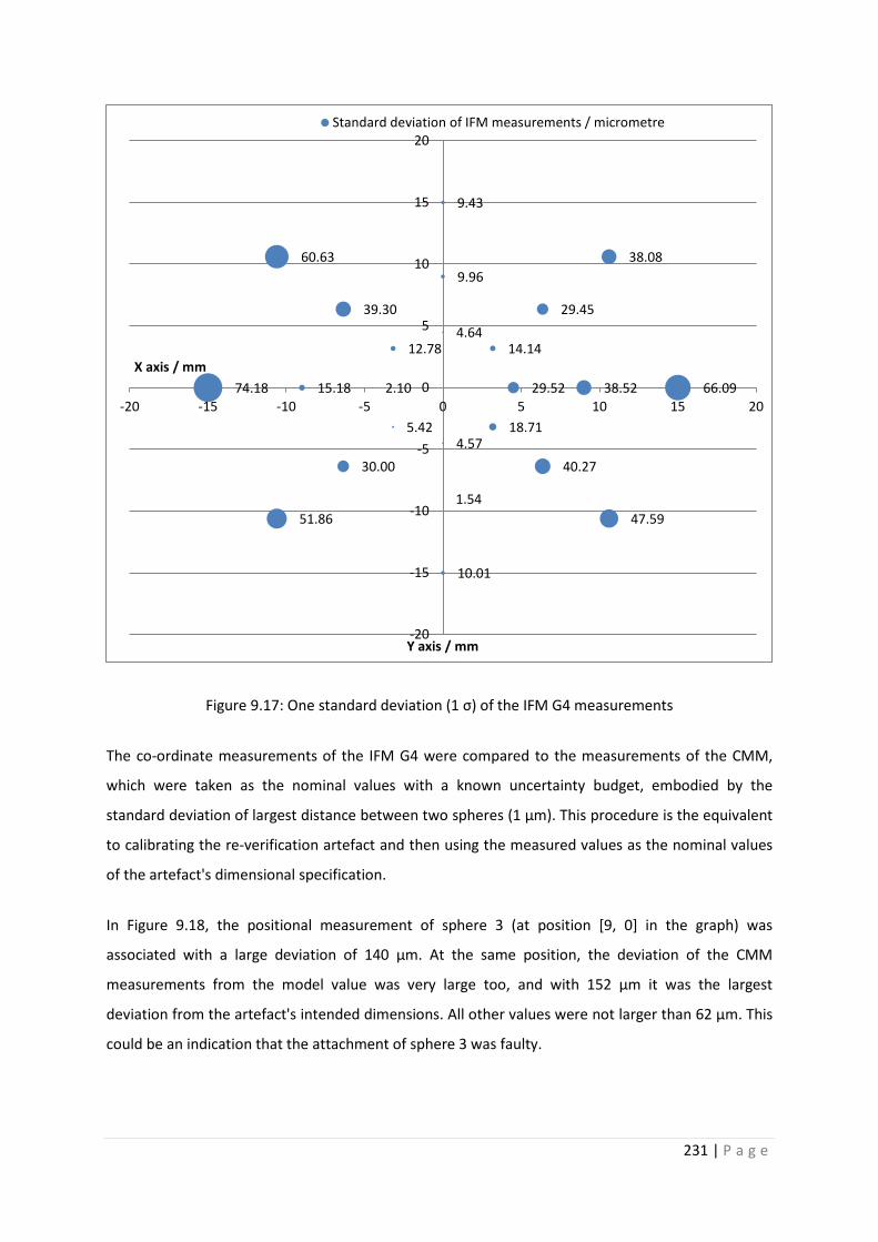
231 | P a g e
Figure 9.17: One standard deviation (1 σ) of the IFM G4 measurements
The co-ordinate measurements of the IFM G4 were compared to the measurements of the CMM,
which were taken as the nominal values with a known uncertainty budget, embodied by the
standard deviation of largest distance between two spheres (1 μm). This procedure is the equivalent
to calibrating the re-verification artefact and then using the measured values as the nominal values
of the artefact's dimensional specification.
In Figure 9.18, the positional measurement of sphere 3 (at position [9, 0] in the graph) was
associated with a large deviation of 140 μm. At the same position, the deviation of the CMM
measurements from the model value was very large too, and with 152 μm it was the largest
deviation from the artefact's intended dimensions. All other values were not larger than 62 μm. This
could be an indication that the attachment of sphere 3 was faulty.
29.52 38.52 66.09
4.64
9.96
9.43
2.10 15.18 74.18
4.57
1.54
10.01
14.14
29.45
38.08
12.78
39.30
60.63
5.42
30.00
51.86
18.71
40.27
47.59
-20
-15
-10
-5
0
5
10
15
20
-20 -15 -10 -5 0 5 10 15 20
X axis / mm
Y axis / mm
Standard deviation of IFM measurements / micrometre

232 | P a g e
Likewise with the standard deviation of the IFM G4 measurements, the deviations from the co-
ordinates measured with the CMM became increasingly larger the further away the spheres were
from the origin, with a mean increase of 385 % (disregarding the outlier in the XZ orientation). This
observation confirms that the IFM G4's XY stage positional error increased linearly, as seen before in
Chapter 8. It was noticeable that the standard deviations of the IFM G4 measurements were larger
than the co-ordinate value deviation from the CMM measurements, as well as the increase of value
when measuring sphere centres further from the origin.
Figure 9.18: Deviation of IFM G4 sphere position measurements from the calibrated values
The following three Figures (Figure 9.19, 9.20, 9.21) present the deviations of each axis (X, Y and Z).
As anticipated the largest deviations from the calibrated values are cause by the XY table, and in
particular from its Y axes. This observation is in agreement with the experimental results of the
positional accuracy tests. Only the smallest deviations are associated with the Z axis.
140.00 34.47
14.41
11.07
19.32
13.38 42.17 61.91
4.08
6.26
9.37
12.19
38.92
13.44
27.32
53.77
7.18
28.56
50.98
14.32
16.82
48.59
-20
-15
-10
-5
0
5
10
15
20
-20 -15 -10 -5 0 5 10 15 20
X axis / mm
Y axis / mm
Deviation of IFM G4 from CMM results / micrometres

233 | P a g e
Figure 9.19: Deviation of IFM G4 sphere position measurements from the calibrated values
38.010 8.733
4.735
5.827
8.996
1.647 7.092 5.534
1.618
1.725
2.412
5.419
16.000
2.002
8.589
13.998
3.926
6.195
8.163
8.275
6.097
4.218
-20
-15
-10
-5
0
5
10
15
20
-20 -15 -10 -5 0 5 10 15 20X axis / mm
Y axis / mm
Deviation of IFM from CMM X axis results / micrometers
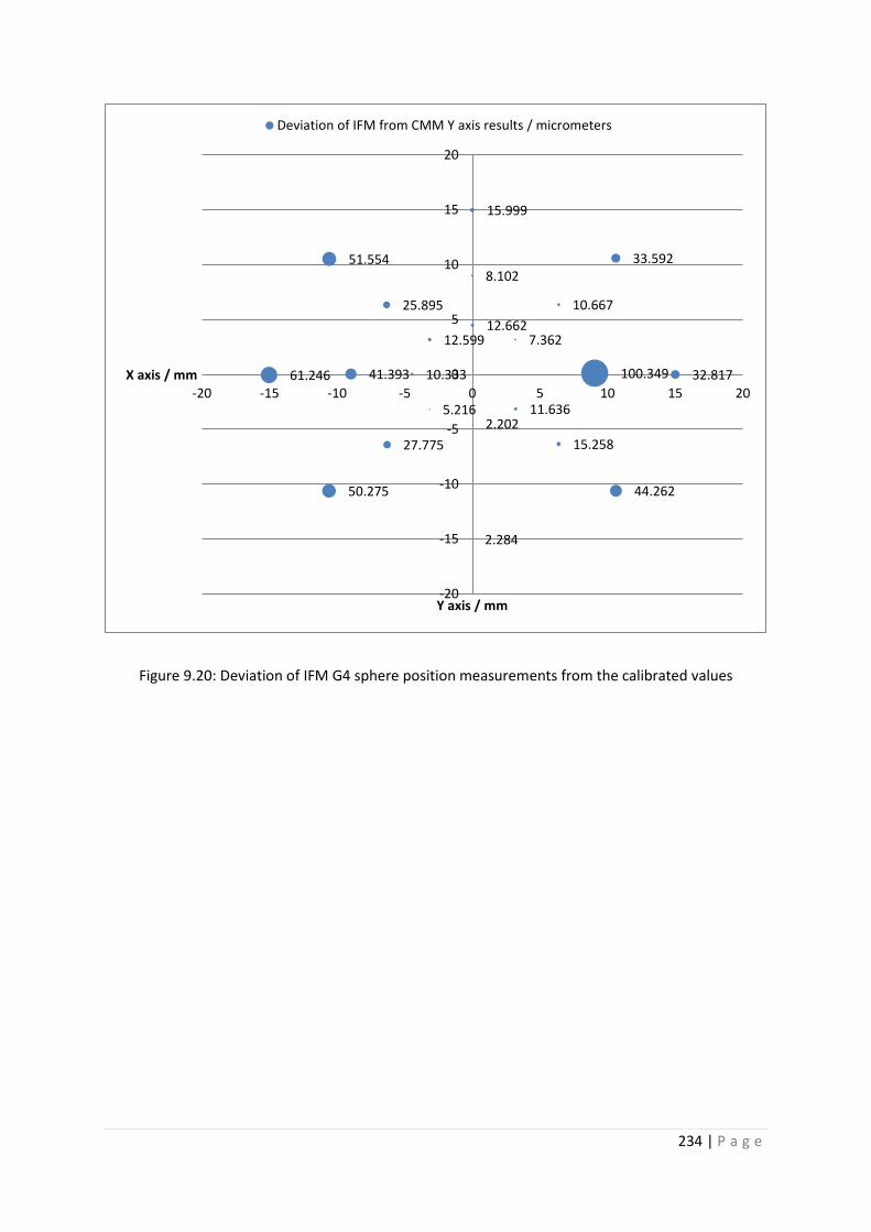
234 | P a g e
Figure 9.20: Deviation of IFM G4 sphere position measurements from the calibrated values
100.349 32.817
12.662
8.102
15.999
10.333 41.393 61.246
2.202
2.284
7.362
10.667
33.592
12.599
25.895
51.554
5.216
27.775
50.275
11.636
15.258
44.262
-20
-15
-10
-5
0
5
10
15
20
-20 -15 -10 -5 0 5 10 15 20X axis / mm
Y axis / mm
Deviation of IFM from CMM Y axis results / micrometers

235 | P a g e
Figure 9.21: Deviation of IFM G4 sphere position measurements from the calibrated values
Applicability of Artefact Fritz for ISO 10360-8
The objective of designing Artefact Fitz was to realise a re-verification artefact that conformed to ISO
10360-8. Consequently it was necessary to demonstrate the applicability of Artefact Fritz for a re-
verification performed with the IFM G4. The co-ordinate measurements that have been presented
above have been used to calculate the distances between spheres in the radial orientations.
Consequently eight sets of six size measurements (a-f, see Figure 9.3) could be calculated for each
set of measurements of all 25 spheres. This resulted in three measurement values for each
measured length and standard deviation values. Because the same set of measurements was used
as for the previous section, the same sources of error apply to this set of results too (e.g. improper
measurement set-up).
ISO 10360-8 suggests that the size measurement deviations for each measurement direction are
presented in a graph as shown in the example in Figure 9.19. The two red lines shown in the figure
90.367 5.900
5.000
4.800
6.033
8.333 3.867 7.167
3.033
5.567
5.267
2.333
11.400
4.233
1.400
6.100
3.000
2.433
2.200
1.100
3.600
19.600
-20
-15
-10
-5
0
5
10
15
20
-20 -15 -10 -5 0 5 10 15 20X axis / mm
Y axis / mm
Deviation of IFM from CMM Z axis results / micrometers

236 | P a g e
are a function of the manufacturer’s MPEE statement, which for the IFM G4 is not given because it is
a surface texture measuring instrument. In Figures 9.23 to 9.30 the measurement errors are
presented in a graph similar to the one shown in Figure 9.22 but without an indication of a MPEE for
the eight radial measurement directions.
It was observed that there was a weak correlation (Pearson, mean correlation = 0.703) between
each set of six measurements in the eight different orientations. This correlation indicates the
presence of a systematic error, which may have been due to the measurement method. The largest
error was 19.4 μm, which in the context of micro-CMMs is a very large measurement deviation,
although possibly an influenced by human error.
Figure 9.22: Representation of size measurement error according to ISO 10360
Figure 9.23: Size measurement error in X(-Z) (± 1 σ)
-20-15-10
-505
101520
0 2 4 6 8
Devi
atio
n /
μm
Length / mm
X(-Z)

237 | P a g e
Figure 9.24: Size measurement error in XY(-Z) (± 1 σ)
Figure 9.25: Size measurement error in Y(-Z) (± 1 σ)
Figure 9.26: Size measurement error in (-X)Y(-Z) (± 1 σ)
-20-15-10
-505
101520
0 5 10 15 20
Devi
atio
n /
μm
Length / mm
XY(-Z)
-20-15-10
-505
101520
0 5 10 15 20
Devi
atio
n /
μm
Length / mm
Y(-Z)
-20-15-10
-505
101520
0 5 10 15 20
Devi
atio
n /
μm
Length / mm
(-X)Y(-Z)
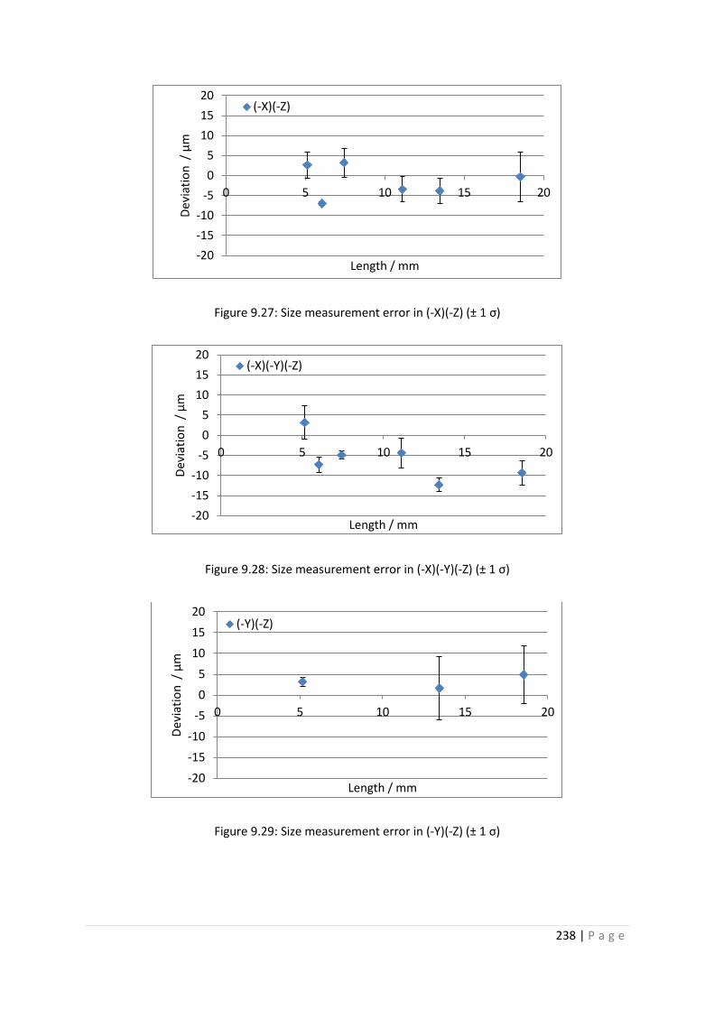
238 | P a g e
Figure 9.27: Size measurement error in (-X)(-Z) (± 1 σ)
Figure 9.28: Size measurement error in (-X)(-Y)(-Z) (± 1 σ)
Figure 9.29: Size measurement error in (-Y)(-Z) (± 1 σ)
-20-15-10
-505
101520
0 5 10 15 20De
viat
ion
/ μm
Length / mm
(-X)(-Z)
-20-15-10
-505
101520
0 5 10 15 20
Devi
atio
n /
μm
Length / mm
(-X)(-Y)(-Z)
-20-15-10
-505
101520
0 5 10 15 20
Devi
atio
n /
μm
Length / mm
(-Y)(-Z)

239 | P a g e
Figure 9.30: Size measurement error in X(-Y)(-Z) (± 1 σ)
9.6.3 Conclusions
Three investigations have been reported here: the calibration of Artefact Fritz, the investigation of
sphere position measurements with the IFM G4, and size measurement error assessment with the
IFM G4 conforming to ISO 10360-8 using Artefact Fritz.
CMM measurement deviations from the design specification were in general not more than 70 μm,
with two exceptions beyond that. A small part of these deviations account for measurement error of
the CMM and the positioning errors of the manufacturing process. However, human error may
account for the largest part of the error: the placement of adhesive and the spheres were completed
manually without the help of magnifying lenses. If the process of placing the sphere was too slow,
then part of the adhesive may have hardened, and the sphere would not have been placed in
contact with the edge of the 0.5 mm diameter hole. The error introduced by misplacing a sphere can
equally affect the X, Y and Z location.
The standard deviations of co-ordinate measurements with the CMM ranged from 136 nm to
616 nm, averaging 409 nm. They showed no relationship between the corresponding co-ordinate
deviations from the design. This observation was positive for the outcome of the measurements,
giving the co-ordinate measurements more credibility. In addition, no relationship was observed
between the sphere’s distance from the origin and the measurement’s standard deviation.
The sphere centre positions of the novel re-verification Artefact Fritz were measured with the IFM
G4. The results confirmed the expectation that the measurement standard deviations of the outer
spheres (on the 30 mm PCD) would be larger than the rest. The reason for this result is the manner
with which the measurements were conducted: successive measurements were completed along
-20-15-10
-505
101520
0 5 10 15 20De
viat
ion
/ μm
Length / mm
X(-Y)(-Z)

240 | P a g e
the virtual line from the sphere at the centre (origin). Thus the accumulated error would be largest
for the furthest sphere from the origin. The results showed that on average the increase was by a
factor of 7.5. The two largest standard deviations were associated with the measurement of the two
outer spheres on the X axis. Measurement in the YZ orientation differed from the other orientations
as their standard deviations were all very low and the increase particularly small (by a factor of 2).
This result was not in agreement with the results of the positional accuracy assessment of the
translational stages of the IFM G4, which showed that the X axis had a smaller positional error.
A comparison between the Metris Ultra CMM and the IFM G4 co-ordinate measurements showed
that the IFM G4’s measurement deviations from the CMM's measurements (without including the
outlier) were on average the same compared to the standard deviation associated with the IFM G4’s
measurements. The measurement standard deviation and the positional accuracy could be
improved for the FV micro-CMM by using higher quality encoders and slide ways for the X and Y
axes.
The measured positions of the spheres of Artefact Fritz were also evaluated with respect to size
measurements as suggested in ISO 10360-8. The results showed that with the IFM G4 the
requirements for size error assessment, as suggested in ISO 10360-8, could be fulfilled using Artefact
Fritz. This means that a calibrated standard specific for the acceptance and re-verification process of
FV micro-CMMs was developed successfully, however, the measurement method would need to be
improved in order to increase the measurement accuracy.
A health checking process using the re-verification artefact was suggested to be three repeated
measurements of the top sphere and four spheres on the outer most PCD (on the body diagonals),
thus the longest distances in all four body-diagonal orientations are measured. The measurement
results are given in Table 9.3.
Table 9.3: Health check test results
Orientation Deviation
(μm)
Standard deviation
(μm)
XY(-Z) 19.4 2.8
(-X)Y(-Z) 1.9 1.8
(-X)(-Y)(-Z) -9.3 2.9
X(-Y)(-Z) 11.2 21
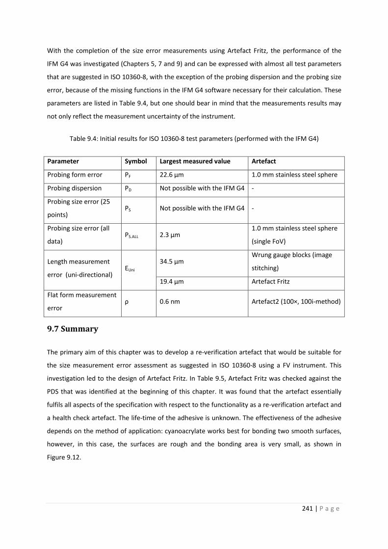
241 | P a g e
With the completion of the size error measurements using Artefact Fritz, the performance of the
IFM G4 was investigated (Chapters 5, 7 and 9) and can be expressed with almost all test parameters
that are suggested in ISO 10360-8, with the exception of the probing dispersion and the probing size
error, because of the missing functions in the IFM G4 software necessary for their calculation. These
parameters are listed in Table 9.4, but one should bear in mind that the measurements results may
not only reflect the measurement uncertainty of the instrument.
Table 9.4: Initial results for ISO 10360-8 test parameters (performed with the IFM G4)
Parameter Symbol Largest measured value Artefact
Probing form error PF 22.6 μm 1.0 mm stainless steel sphere
Probing dispersion PD Not possible with the IFM G4 -
Probing size error (25
points) PS Not possible with the IFM G4 -
Probing size error (all
data) PS.ALL 2.3 μm
1.0 mm stainless steel sphere
(single FoV)
Length measurement
error (uni-directional) EUni
34.5 μm Wrung gauge blocks (image
stitching)
19.4 μm Artefact Fritz
Flat form measurement
error ρ 0.6 nm Artefact2 (100×, 100i-method)
9.7 Summary
The primary aim of this chapter was to develop a re-verification artefact that would be suitable for
the size measurement error assessment as suggested in ISO 10360-8 using a FV instrument. This
investigation led to the design of Artefact Fritz. In Table 9.5, Artefact Fritz was checked against the
PDS that was identified at the beginning of this chapter. It was found that the artefact essentially
fulfils all aspects of the specification with respect to the functionality as a re-verification artefact and
a health check artefact. The life-time of the adhesive is unknown. The effectiveness of the adhesive
depends on the method of application: cyanoacrylate works best for bonding two smooth surfaces,
however, in this case, the surfaces are rough and the bonding area is very small, as shown in
Figure 9.12.

242 | P a g e
Table 9.5: Checking the design of Artefact Fritz against PDS
Product specification Artefact Fritz
The artefact should be an easily manageable
object, in terms of approach and weight
(< 800 g).
The base of the artefact can be held easily. Weight:
622 g.
The artefact should not be larger than 75
mm × 75 mm × 75 mm.
The artefact is 50 mm wide and 65 mm tall.
The artefact material’s thermal expansion
coefficient should be less than 20 × 10-6 / K.
The artefact is made of stainless steel with a thermal
expansion coefficient of 16 × 10-6 / K.
The artefact design should appear to be
simple.
This was achieved by designing the artefact
cylindrically symmetric.
Its functionality should be intuitive by its
design.
Marked X and Y orientations are required to fulfil this
specification. Otherwise, its functionality is intuitive.
The re-verification procedure performed
with this artefact should be as similar as
possible to the size error measurement
procedure presented in ISO 10360-8.
Six different calibrated lengths can be measured in
the XZ, YZ orientations, and variants of the XYZ
orientations. (5.151 mm, 5.966 mm, 7.405 mm,
11.123 mm, 13.370 mm, 18.527 mm). It is also
possible to measure five horizontally orientated
lengths (i.e. X and Y).
The measurement uncertainty of the
artefact calibration should be better than
50 nm.
This specification could not be achieved with the
Metris Ultra CMM. The mean measurement standard
deviation (1 σ) was 452 nm. A better measurement
standard deviation would be given with the Zeiss F25
micro-CMM.
The measurement accuracy of the artefact
calibration should be better than 100 nm.
The measurement accuracy for the longest length
measured was 21 nm (calculated by using the MPEE
statement for the Metris Ultra) plus the accuracy of
measuring the sphere centre, which is unknown
here.
The artefact should have a lifetime of 10
years.
Dependent on the adhesive and the application of
the adhesive.
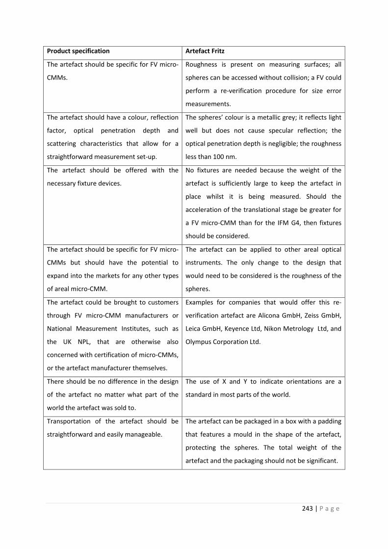
243 | P a g e
Product specification Artefact Fritz
The artefact should be specific for FV micro-
CMMs.
Roughness is present on measuring surfaces; all
spheres can be accessed without collision; a FV could
perform a re-verification procedure for size error
measurements.
The artefact should have a colour, reflection
factor, optical penetration depth and
scattering characteristics that allow for a
straightforward measurement set-up.
The spheres’ colour is a metallic grey; it reflects light
well but does not cause specular reflection; the
optical penetration depth is negligible; the roughness
less than 100 nm.
The artefact should be offered with the
necessary fixture devices.
No fixtures are needed because the weight of the
artefact is sufficiently large to keep the artefact in
place whilst it is being measured. Should the
acceleration of the translational stage be greater for
a FV micro-CMM than for the IFM G4, then fixtures
should be considered.
The artefact should be specific for FV micro-
CMMs but should have the potential to
expand into the markets for any other types
of areal micro-CMM.
The artefact can be applied to other areal optical
instruments. The only change to the design that
would need to be considered is the roughness of the
spheres.
The artefact could be brought to customers
through FV micro-CMM manufacturers or
National Measurement Institutes, such as
the UK NPL, that are otherwise also
concerned with certification of micro-CMMs,
or the artefact manufacturer themselves.
Examples for companies that would offer this re-
verification artefact are Alicona GmbH, Zeiss GmbH,
Leica GmbH, Keyence Ltd, Nikon Metrology Ltd, and
Olympus Corporation Ltd.
There should be no difference in the design
of the artefact no matter what part of the
world the artefact was sold to.
The use of X and Y to indicate orientations are a
standard in most parts of the world.
Transportation of the artefact should be
straightforward and easily manageable.
The artefact can be packaged in a box with a padding
that features a mould in the shape of the artefact,
protecting the spheres. The total weight of the
artefact and the packaging should not be significant.

244 | P a g e
Product specification Artefact Fritz
Transport protection should be simple, and
it should ideally present the artefact to the
user.
The box in which the artefact is packaged can be
manufactured to ideally present the artefact.
The artefact should have at least one set of
five different lengths in order to establish
the size measurement error of a FV micro-
CMM conforming to ISO 10360-8.
The artefact features eight sets of four spheres in a
row. Between the four sphere centres, six lengths
can be measured.
Defined lengths must be measurable in at
least seven different orientations, of which
four must be body-diagonals.
Size measurements with Artefact Fritz can be
completed in all four body-diagonals, and
additionally the X, Y, XY, XZ, and YZ orientations.
The re-verification process should be as
short as possible, approximately one day.
The size measurement error assessment can be
completed in approximately 7h 30min. Added to that
is the time needed for the probe error
measurements, which could be completed within 30
minutes (see Section 8.3.4.1). The complete re-
verification of a FV instrument procedure should not
take more than one day.
A health check procedure using the artefact
should be able to be performed within
approximately 30 minutes.
A health check procedure could be completed within
one hour, if only five spheres are measured
repeatedly for the size measurement error
assessment.
All measurement points must be well
defined.
The sphere centre can be measured with one FoV
with a standard deviation of up to 74.6 μm. The
uncertainty budget can be decreased by improving
the measuring method and the sphere fitting
function.
The measurement points should not be
easily influenced by temperature, humidity
or noise.
Temperature affects all spheres in the same manner.
The stainless steel substrate acts as a heat sink. The
effect of humidity on the spheres’ surface
measurements is unknown. The effect of noise on
the geometric measurements of angled surfaces is
negligible as was seen in Chapter 5.

245 | P a g e
Product specification Artefact Fritz
The artefact should have a random
roughness that is the same at all
measurement locations and approximately
30 nm Ra.
Grade 100 spheres were used, which had a
roughness (Ra) of approximately 100 nm as a result
of the manufacturing process.
The number of measurements should be
kept to a minimum but conform to ISO
10360-8.
A minimum of 21 spheres must be measured to
conform to the size measurement error assessment
stated in ISO 10360-8.
A re-verification of the vertical axis (without
moving the YX stage) can only be completed
with small step heights.
Step heights that can be measured within one FoV
are not featured by Artefact Fritz.
The artefact’s manufacturing should be
uncomplicated.
The base of the artefact can be realized using a lathe
and a drill, and the spheres must be lapped to a
specific surface roughness. These are well-known
methods in manufacturing engineering. The method
for applying the adhesive and locating the spheres
needs to be refined.
The product should be robust to vibrations
and handling.
Care should be taken when contacting the spheres,
otherwise the artefact is robust to handling. The
artefact has no feature that mitigates vibrations from
the environment.
The artefact should be easy to measure with
a low risk of collision of the objective lens
and the object
There is a medium risk of colliding the lens with the
artefact, and requires care when defining the co-
ordinate space of the artefact within the measuring
volume of the FV micro-CMM. An automated re-
verification procedure can lower the risk of collision.
It should be easy to clean. The lower side of the spheres may be difficult to
clean, but these areas are not used for the re-
verification procedure.
The artefact should be heavy enough not to
move when being measured
The weight of Artefact Fritz is sufficient for the
artefact not to move during the measurement
procedure with respect to the XY stage.

246 | P a g e
Chapter 10: Conclusions and further work
10.1 Conclusions
The aim of this thesis was to investigate the potential of the focus variation technique to be
developed as a micro-CMM platform. The core objectives of this research project, as previously
identified in Chapter 1, were to:
• Understand the necessity of implementing a new technique as a micro-CMM platform that
can offer advantages over other techniques currently used for micro-CMMs.
• Understand how the FV technique works, its drawbacks and advantages over other areal
optical instruments.
• Explore methods of assessing performance characteristics in terms of measurement noise
and residual flatness, and simultaneously to explore the influence of instrument settings on
these performance characteristics.
• Explore the performance characteristics of the FV technique for high aspect ratio surface
measurements as this is one of the key advantages that this technique has over other optical
techniques.
• Assess the capability of the FV technique to perform basic geometric measurements.
• Assess the capability of the FV technique positional accuracy with the view to using this
instrument as a micro-CMM.
• Explore a traceable route to link the FV technique performance with the definition of the
metre, in the context of co-ordinate measurement (i.e. acceptance, re-verification and
health check tests).
• Identify a suitable re-verification (and health check) artefact for a future FV technique based
micro-CMM.
The investigation comprised an assessment of the instrument performance characteristics based on
a commercial FV system designed for surface texture measurements, the Alicona GmbH IFM G4. The
research also investigated simple geometric measurements to evaluate the potential for accurate
geometric measurements using the FV technique. Suggestions were given for an acceptance and a
re-verification, and health checking procedure, based on the existing ISO 10360-8 but designed
specifically for FV micro-CMMs. In connection with this procedure, a re-verification artefact design
was presented that has the potential to be used by FV micro-CMM users to regularly assess the
instrument performance.

247 | P a g e
Figure 10.1 shows how the surveys of literature and the information gained from the experimental
work led to the suggestion of an acceptance and re-verification procedure and a heath check test,
and finally to the re-verification artefact. It gives an indication on the level of novelty of each
investigation.
Figure 10.1: Novelty factors
The investigation of instrument performance characteristics of the IFM G4 was successfully
completed. It comprised the assessment of measurement noise (Chapter 4), residual flatness
(Chapter 5) and high aspect texture measurements (Chapter 6). The primary conclusions from the
elements of work can be summarised as follows:
248 | P a g e
• The measurement noise was assessed for all six lenses (2.5×, 5×, 10×, 20×, 50×, and 100×) of
the IFM G4 instrument by using a subtraction technique. This first investigation showed that
the measurement noise level had an approximately exponential relationship with the lens
magnification: lower lens magnifications were affected by a higher measurement noise level.
The measurement noise assessment was extended to investigate the effect of variable
measurement settings on measurement noise. The results showed that typically a short
exposure time increased the measurement noise by 88 % whilst a long exposure time
decreased the measurement noise by 22 %. The contrast did not have a significant effect on
measurement noise. A low vertical resolution and a high lateral resolution affected the
measurement noise negatively (increase of noise by 98 % and 46 %, respectively), whilst a
low lateral resolution and a high vertical resolution affected the measurement noise
positively (reduction of noise by 44 % and 42 %, respectively).
• The residual flatness of the IFM G4 was assessed for the lenses with magnifications 10×, 20×,
50× and 100×, which are the main lenses used for surface texture measurements, using
three variations of an averaging technique that was previously developed by NPL (UK) for
surface texture measuring instruments capable of measuring optical flat surfaces. The first
variation used a roughened artefact (approximate Ra = 30 nm) instead of an optical flat and
it was found that the averaging technique using ten images did not produce information that
was representative of the residual flatness (Szflatness was 12.2 nm, 100× lens).
• The second variation of the averaging technique used the roughened surface and applied a
waviness filter to the averaged stack of ten images producing significantly lower residual
flatness values than the first method (Szflatness was 2.0 nm, 100× lens). The third method used
100 images instead of only 10 images of the roughened surface. In general this method
produced the smallest value for the residual roughness of the system (Szflatness was 0.6 nm,
100× lens). The results of the two latter methods were comparable in terms of numerical
values of the lenses that were investigated. The numerical results for the 100× lens are
summarized in Table 10.1.

249 | P a g e
Table 10.1: Summary of residual flatness results (100× lens)
Method Szflatness
(nm)
10i 12.2
10if 2.0
100i 0.6
• High aspect ratio measurements of a roughened (Ra = 25.3 nm) surface were investigated
for different combinations of measurement settings. The combinations of settings were as
follows: coaxial illumination only; coaxial and ring-light illuminations; coaxial and lateral
resolution compensation; coaxial and ring-light illuminations and a polariser. The
conclusions drawn from the results were that the ring-light illumination made an
insignificant difference to the surface characterisation (in terms of Sq) of high aspect ratio
surfaces. The polariser and the lateral resolution compensation both made positive
differences for angles above the lens’ numerical half apertures.
• A high aspect ratio measurement comparison was conducted for three surfaces: one
sinusoidal roughened surface (Ra = 500 nm), and two flat randomly roughened surfaces with
different roughness values (Ra = 25.3 nm and Ra = 42.7 nm). The sinusoidal surface
measurement was assessed in terms of Ra because the surface was not homogeneously
roughened. These roughness measurements of the sinusoidal surface had a deviation of less
than 22 nm from the nominal at all angles up to 55 degrees. The latter showed that the
presence of a sinusoidal structure on a surface improves the quality of high aspect ratio
measurements because the structure provides the surface with a larger roughness, for
which the FV instrument was designed to measure. Conclusions from the high aspect
measurements with flat micro-roughened artefacts were that the Sq parameters of a
rougher surface could be measured better than a comparable surface with a slightly smaller
roughness.
An important objective that was successfully achieved was to assess the potential of the FV
technique to be transformed into a FV micro-CMM. For this assessment the IFM G4 was tasked with
measurements of geometric features: angles, distances and sphere radii. These are reported in
Chapter 7. The conclusions of these geometric measurement results are as follows:
250 | P a g e
• The angle measurements were completed by measuring a roughened (Ra = 25.3 nm) gauge
block at angles from 0 degrees to 80 degrees in increments of 5 degrees and to then use the
effective surfaces to calculate the angle between the plane fitted to the data and the
measurement volume's horizontal plane. The results showed that all error sources that
influenced the angle measurements did not introduce an error of larger than 0.2 degrees,
although it should be noted that this statement is based on disregarding one outlying data
point as a function of error. The standard deviations of the three measurements of each
angle were approximately increasingly larger for angles up to 55 degrees. For higher angles,
the standard deviations were lower. The angles measured with the highest standard
deviations (0.35 degrees) were around the half aperture angle of the 100x objective lens
used for all measurement.
• Distance measurements were performed using gauge blocks (1.0 mm, 3.0 mm, 4.0 mm,
8.0 mm, and 16.0 mm). These were set up with three different methods: by wringing all
together, by pushing them together in a gauge block holder so that the edges of the gauge
blocks were staggered, and by simply pushing the gauge blocks together without staggered
edges. Line measurements over all gauge blocks were recorded and the results showed that
the distance measurement errors were large regardless of the method. The first method
showed the smallest deviations of the three methods (maximum deviation from the nominal
in X and Y, 34 μm and 19 μm) The second method was designed so that partially a gap was
measured in between gauge blocks, and thus the line measurements relied on less data for
the image stitching function. Consequently, the maximum deviations from the nominal in X
and Y were very large, with 79 μm and 102 μm respectively. The third method had slightly
smaller deviations than the second method (maximum deviation from the nominal in X and
Y, 78 μm and 59 μm). Overall the gauge block measurements were successful in
demonstrating that gauge blocks are not ideal for length measurements with a FV system
and that edge detection is an issue that needs improving when developing a FV micro-CMM.
• The last of the simple geometric measurements were the sphere radius measurements,
which aimed to investigate how well the IFM G4 would measure different types of materials,
and different roughness and different radii. The four chosen materials were ruby (aluminium
oxide, grade 5), zirconia (grade 3), silicon nitride (grade 5), and stainless steel (Grade 100).
The different sizes were 2.0 mm, 1.0 mm, and 0.5 mm diameter. A comparison between
measurements of 1.0 mm spheres for all materials showed that the mean radius
measurements of the ruby spheres had a large deviation from the 500 μm nominal value

251 | P a g e
(507 μm) and a large standard deviation (20.4 nm), the zirconia spheres also had a large
measurement deviation from the 500 μm nominal but the associated standard deviation was
smaller (0.8 nm).
• Radius measurements of the 1.0 mm silicon nitride spheres showed a smaller measurement
deviation from the nominal (4.0 μm) and a small standard deviation (2.3 μm), and
measurements of the stainless steel spheres showed that the measurement deviation was
very small (1.0 μm) and that the associated standard deviation was 3.3 nm. The stainless
steel sphere measurements did not perform best, but they were good enough to use them
for the re-verification artefact.
• Differently sized zirconia spheres (2.0 mm, 1.0 mm, 0.5 mm) were measured with the aim to
assess how the sphere size affects the measurement quality in terms of measurement
variation (1 σ). The results showed that the measurement deviation relative to the nominal
radius was smallest for the 1.0 mm sphere with 1 σ = 3.0 μm. This result indicated that
1.0 mm spheres were a suitable size for a re-verification artefact. A comparative study of the
use of a single FoV and multiple FoVs (image field) was conducted with 1.0 mm zirconia
spheres and stainless steel spheres. The conclusion drawn from both sets of measurements
was that using an image field did not make the measurement deviations smaller but the
measurements were more repeatable (maximum 1 σ of single FoV measurements: 2.0 μm;
maximum 1 σ of single FoV measurements: 3.3 μm).
The FV instrument, IFM G4, was examined with respect to its functionality as a micro-CMM based on
the FV technique and missing features were identified. Another primary objective was to investigate
how a manufacturer of a FV micro-CMM could provide evidence that the instrument performs
within the given specifications and how a user could re-verify that the instrument subsequently
conforms to the instrument specification (re-verification and health check). These objectives were
successfully achieved in Chapters 8 and 9, of which the conclusions are as follows:
• The changes that would have to be made to the IFM G4 are summarized in Table 10.2.

252 | P a g e
Table 10.2: Changes to the IFM G4 to develop a FV micro-CMM
IFM G4 FV micro-CMM
Structure Column-bridge with XY stage Column-bridge with XY stage
XY stage encoders unknown Optical encoders
XY stage accuracy Up to 16.87 μm Below 250 nm
Rotary axis Existing feature Should be part of micro-CMM
Objective lenses 2.5× to 100× 2.5× to 100×
Measurement noise Up to 40 nm for 10× Below 50 nm
Flatness error Up to 7.3 nm for 10× Below 5 nm
Vibration isolation system Passive Passive
CAD kernel Not existing Must be integrated
CAD software Not existing Must be integrated
Object weight Limited to 35 kg Limit is dependent on XY
stage
Areal size of features to be
measured 100 mm × 100 mm 100 mm × 100 mm
Datum alignment Not existing Must be integrated
Acceptance and re-
verification - Must be specified
Health check Chess-board artifact and step height Must be specified
• The positional accuracy assessment of the IFM G4 was measured with a Renishaw ML 10
interferometer system using the ISO 230-2 specification by placing one mirror onto the
movable XY stage and by measuring the deviation of each axial positioning at six nominal
values. The results showed that the X and Y directional accuracies to be 14.41 μm and
16.87 μm, respectively. A summary of the positional accuracy data for the XY stage is
presented in Table 10.3. These results showed a good performance, however, it must be
taken into consideration that the IFM G4 was not intended to have highly accurate
horizontal positioning because distance measurements were supposed to rely on image
stitching. The stage accuracy should not be confused with the instrument accuracy. The Z
axis was also investigated; however, the mounting of the mirror to the Z axis could not be
achieved well without damaging the instrument and a non-representative creep presented
itself in the measurements of the Z positional accuracy.
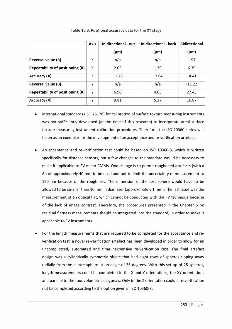
253 | P a g e
Table 10.3: Positional accuracy data for the XY stage
Axis Unidirectional - out
(μm)
Unidirectional - back
(μm)
Bidirectional
(μm)
Reversal value (B) X n/a n/a 1.97
Repeatability of positioning (R) X 2.05 1.39 6.39
Accuracy (A) X 11.78 12.64 14.41
Reversal value (B) Y n/a n/a -11.22
Repeatability of positioning (R) Y 6.90 4.05 27.45
Accuracy (A) Y 9.81 5.27 16.87
• International standards (ISO 25178) for calibration of surface texture measuring instruments
was not sufficiently developed (at the time of this research) to incorporate areal surface
texture measuring instrument calibration procedures. Therefore, the ISO 10360 series was
taken as an exemplar for the development of an acceptance and re-verification artefact.
• An acceptance and re-verification test could be based on ISO 10360-8, which is written
specifically for distance sensors, but a few changes to the standard would be necessary to
make it applicable to FV micro-CMMs. One change is to permit roughened artefacts (with a
Ra of approximately 40 nm) to be used and not to limit the uncertainty of measurement to
150 nm because of the roughness. The dimension of the test sphere would have to be
allowed to be smaller than 10 mm in diameter (approximately 1 mm). The last issue was the
measurement of an optical flat, which cannot be conducted with the FV technique because
of the lack of image contrast. Therefore, the procedures presented in the Chapter 5 on
residual flatness measurements should be integrated into the standard, in order to make it
applicable to FV instruments.
• For the length measurements that are required to be completed for the acceptance and re-
verification test, a novel re-verification artefact has been developed in order to allow for an
uncomplicated, automated and time-inexpensive re-verification test. The final artefact
design was a cylindrically symmetric object that had eight rows of spheres sloping away
radially from the centre sphere at an angle of 36 degrees. With this set-up of 25 spheres,
length measurements could be completed in the X and Y orientations, the XY orientations
and parallel to the four volumetric diagonals. Only in the Z orientation could a re-verification
not be completed according to the option given in ISO 10360-8.
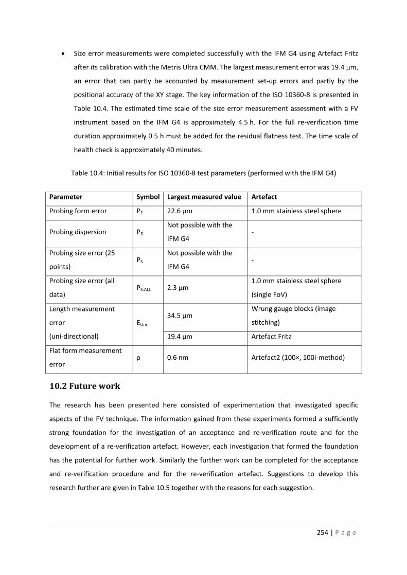
254 | P a g e
• Size error measurements were completed successfully with the IFM G4 using Artefact Fritz
after its calibration with the Metris Ultra CMM. The largest measurement error was 19.4 μm,
an error that can partly be accounted by measurement set-up errors and partly by the
positional accuracy of the XY stage. The key information of the ISO 10360-8 is presented in
Table 10.4. The estimated time scale of the size error measurement assessment with a FV
instrument based on the IFM G4 is approximately 4.5 h. For the full re-verification time
duration approximately 0.5 h must be added for the residual flatness test. The time scale of
health check is approximately 40 minutes.
Table 10.4: Initial results for ISO 10360-8 test parameters (performed with the IFM G4)
Parameter Symbol Largest measured value Artefact
Probing form error PF 22.6 μm 1.0 mm stainless steel sphere
Probing dispersion PD Not possible with the
IFM G4 -
Probing size error (25
points) PS
Not possible with the
IFM G4 -
Probing size error (all
data) PS.ALL 2.3 μm
1.0 mm stainless steel sphere
(single FoV)
Length measurement
error
(uni-directional)
EUni 34.5 μm
Wrung gauge blocks (image
stitching)
19.4 μm Artefact Fritz
Flat form measurement
error ρ 0.6 nm Artefact2 (100×, 100i-method)
10.2 Future work
The research has been presented here consisted of experimentation that investigated specific
aspects of the FV technique. The information gained from these experiments formed a sufficiently
strong foundation for the investigation of an acceptance and re-verification route and for the
development of a re-verification artefact. However, each investigation that formed the foundation
has the potential for further work. Similarly the further work can be completed for the acceptance
and re-verification procedure and for the re-verification artefact. Suggestions to develop this
research further are given in Table 10.5 together with the reasons for each suggestion.

255 | P a g e
Table 10.5: Future work
Work completed Future work Reasons for future work
Measurement noise To distinguish measurement noise
in vibrational noise components,
electronic noise, software noise
(error induced by the calculation of
contrast);
To improve the technique of
assessing measurement noise;
To investigate the different between
the addition and the subtraction
methods for noise measurements of
FV instruments
The information gained from the
different noise components could
provide evidence to further improve
the instrument hardware and
software.
This improvement would diminish the
measurement uncertainty.
Whilst the methods are approximately
equally good for other imaging
methods, there may be a difference
for FV instruments.
Residual flatness Development and testing of an
automatic residual flatness
procedure;
It is essential for the completion of a
re-verification test within a shorter
period of time compared to the 100i-
method. It would also minimise
human error.
High aspect ratio
surface texture
measurements
Improvement of measurements of
high aspect ratio surfaces;
This would give more accurate
information of the surface in terms of
profile and surface parameters.
Angle
measurements
using angle gauges
Angle measurement deviation; It could be used as a method of
investigating the Z axis’ accuracy (an
under-estimation of the angle points
towards positive positional deviation,
and vice versa).
Length
measurements
using gauge blocks
Improvement of the accuracy of
locating the surface where there is a
border between information given
and no information (e.g. the edge of
a gauge block where one surface is
at 90 degrees);
This improvement would have an
impact on for example diameter
measurements of micro-holes.

256 | P a g e
Work completed Future work Reasons for future work
Radius
measurements
using spheres
Improvement of shape fitting
procedures, in order to make them
more robust with respect to
measurement noise, spikes and data
loss;
This would improve the accuracy of
distance measurement between two
sphere centres.
Acceptance, re-
verification and
health checking
procedures
Integration of a standard specific for
areal micro-CMMs in the ISO 10360
suite, or the revision of ISO 10360 to
cover FV;
To be able to follow an acceptance, re-
verification and health checking
procedure specifically written for FV
micro-CMMs would give the user
more confidence than when
compromises to a procedure are met.
Positional accuracy Improvement of the method of
measuring the positional accuracy in
the Z axis, with respect to ISO 230-2;
Comparison between position
accuracy by image stitching and by
XY stage.
This work would be particularly useful
to the instrument manufacturers, if
they decided to provide positional
accuracy of all translational axes with
each instrument.
This would show which method is
better.

257 | P a g e
Work completed Future work Reasons for future work
Re-verification
artefact
Investigation in an improved
method of fixing the spheres to the
artefact;
Designing and testing a method to
calibrate the artefact using the Zeiss
F25 or a micro-CMM with similar
specifications in order to formally
establish a traceable route to the
metre;
Investigation of sphere
measurements of grade 100
stainless steel spheres using the
Zeiss F25.
The artefact has to be more robust to
handling than artefact Fritz.
The artefact is expected to be
accompanied by a very small
uncertainty statement (approximately
50 nm).
The grade 100 stainless steel spheres
may be too rough to be calibrated
with a touch trigger system and they
may need to be replaced by grade 5
silicon nitride spheres.
10.3 A last note on the topic of machines
This thesis started with an extract from a poem from Oliver Wendell Holms (One-hoss Shay) that
described how a one-hoss shay goes to pieces all at once because it was built in such a logical way, in
contrast to a chaise that has a weak spot, and therefore, breaks down and does not wear out.
Metrology is an aid in the manufacturing process to make parts last longer so that the assembly of
parts can “wear out” and not “break down”. The measurement instruments, however, that are built
for part inspections, such as surface topography instruments and CMMs, can only deliver to meet a
certain satisfaction if they have been given the functionality to do so. This thought is reflected in the
poem by Rudyard Kipling, “the secret of the machines” (Kipling, 1943).
The Secret of the Machines
By Rudyard Kipling
We were taken from the ore-bed and the mine,
We were melted in the furnace and the pit—
We were cast and wrought and hammered to design,
We were cut and filed and tooled and gauged to fit.
Some water, coal, and oil is all we ask,

258 | P a g e
And a thousandth of an inch to give us play:
And now, if you will set us to our task,
We will serve you four and twenty hours a day!
We can pull and haul and push and lift and drive,
We can print and plough and weave and heat and light,
We can run and race and swim and fly and dive,
We can see and hear and count and read and write!
But remember, please, the Law by which we live,
We are not built to comprehend a lie,
We can neither love nor pity nor forgive.
If you make a slip in handling us you die!
We are greater than the Peoples or the Kings—
Be humble, as you crawl beneath our rods!-
Our touch can alter all created things,
We are everything on earth—except The Gods!
Though our smoke may hide the Heavens from your eyes,
It will vanish and the stars will shine again,
Because, for all our power and weight and size,
We are nothing more than children of your brain!

259 | P a g e
Chapter 11: References
Aizawa, K., Sakaue, K., Suenaga, Y., 2005. Image Processing Technologies: Algorithms, Sensors,
Applications (Signal Processing), New York: Marcel Dekker, ISBN 0203913493.
Alicona, 2009. New roughness standard - Traceable optical roughness measurements, (online)
Available at: http://www.zeit.alicona.com/home/news/news/Neues-Rauheitsnormal---
Rueckfuehrbare-optische-Rauhei.en.php [Accessed 08 July 2013].
Alicona, 2011. Training Roughness Measurements Basic & Advanced, Alicona GmbH.
Alicona, 2013. Full form measurement with InfiniteFocus Real3D, (online) Available at:
http://www.alicona.com/home/products/InfiniteFocus-Real-3D.en.php, [Accessed 14 March 2013].
American Foundry Society [AFS], 2013. Surface finishes for casting processes, (online) Available at:
http://www.afsinc.org/about/content.cfm?itemnumber=6915), [Accessed 28 June 2013].
Asif, M., Choi, T.S., 2001. Shape from focus using multilayer feed forward neural networks, IEEE
Transactions on Image Processing, Vol. 10 (11), pp. 1670-1675.
Autocad, 2013. 2D and 3D CAD tools for design and documentation, (online) Available at:
http://www.autodesk.co.uk/products/autodesk-autocad/features, [Accessed 24 June 2013].
Baehnisch, C., Stelldinger, P., Koethe, U., 2009. Fast and accurate 3D edge detection for surface
reconstruction, Technical Report, University Heidelberg, (online) Available at: http://hci.iwr.uni-
heidelberg.de/publications/mip/techrep/baehnisch_09_fast.pdf [Accessed 09 December 2013].
Beckmann, E.C., 2006. CT scanning the early days, The British Journal of Radiology, Vol. 79, pp. 5-8.
Bell, F.K., Raleigh, F.L., 1986. Bridge type Coordinate Measuring Machines, Centerville, OH,
US 4610089.
Bennett, J.M., 1976. Measurement of the RMS roughness, autocovariance function and other
statistical properties of optical surfaces using a FECO scanning interferometer, Applied Optics, Vol. 15
(11), pp. 2705-2721.
Bhushan, B., Wyant, J.C., Koliopoulos, C.L., 1985. Measurement of surface topography of magnetic
tapes by Mirau interferometry, Applied Optics, Vol. 24 (10), pp. 1489-1497.

260 | P a g e
Bos, E.J.C., Delbressine, F.L.M, Haitjema, H., 2004. High-accuracy CMM metrology for micro-systems,
Proceedings of IMEKO, pp. 8, Erlangen, Germany.
Bos, E.J.C., 2008. Tactile 3D Probing System for Measuring MEMS with Nanometre Uncertainty:
Aspects of Probing, Design, Manufacturing and Assembly, Eindhoven: Technical University
Eindhoven, ISBN 9789038612164.
Bos, E.J.C., Schellekens, P.H.J., Dietzel, A.H., 2009. Aspects of tactile probing on a micro-scale,
Proceedings of the 9th Euspen International Conference, Vol . 2, pp. 1-4, San Sebastian, Spain.
Bosch, J.A., 1995. Coordinate Measuring Machines and Systems, New York: Marcel Decker, ISBN
0824795814.
BS EN ISO 1, 2002. Geometrical Product Specifications (GPS) — Standard reference temperature for
geometrical product specification and verification, British Standard.
BS ISO 3534-1, 1993. Statistics – Vocabulary and symbols – Part 1: Probability and general statistical
terms, British Standard.
BS 5233, 1986. Terms used in metrology (incorporating BS 2643), British Standard.
BSI PD 6461-1, 1995. Vocabulary of metrology - Part 1: Basic and general terms (international),
British Standard.
BSI PD 6461-2, 1980. Vocabulary of metrology - Part 2: Vocabulary of legal metrology – Fundamental
terms, British Standard.
BS 6808-3, 1989. Coordinate measuring machines - Part 3: Code of practice, British Standard.
BS 7172, 1989. Guide to assessment of position, size and departure from nominal form of geometric
features, British Standard.
BS 7373-2, 2001. Product specification - Part 2: Guide to identifying criteria for a product
specification and to declaring product conformity, British Standard.
Bureau International des Poids et Mesures (BIPM), 2006. The BIPM and the evolution of the
definition of the metre, (online) Available at: http://www.bipm.org/en/si/history-
si/evolution_metre.html, [Accessed 29 May 2013].

261 | P a g e
Busch, K., Kunzmann, H., Waeldele, F., 1985. Calibration of co-ordinate measuring machines,
Precision Engineering, Vol.2 (3), pp.139-144.
Caber, P.J., 1993. Interferometric profiler for rough surfaces, Applied Optics, Vol. 32 (19), pp. 3438-
3441.
Claverley, J.D., Leach, R.L., 2013. Development of a three-dimensional vibrating tactile probe for
miniature CMMs, Precision Engineering, Vol. 37, pp. 491-499.
Coleman, D.R., Waters, T.F., 1997. Fundamentals of Touch Trigger Probing, Havant: Touch Trigger
Press, ISBN 0951201018.
Cowley, A., 2011. A healthy future: platinum in medical applications, Platinum Metals Review, Vol.
55 (2), pp. 98-107.
Dai, G., Pohlenz, F., Danzebring, H.-U., Xu, M., Hasche, K., Wilkening, G., 2004. Metrological large
range scanning probe microscope, Review of Scientific Instruments, Vol. 75 (4), pp.962-969.
Dai, G., Haessler-Grohne, W., Hueser, D., Wolff, H., Danzebrink, H.-U., Koenders, L., Bosse, H., 2011.
Development of a 3D-AFM for true 3D measurement of nanostructures, Journal of Measurement
Science and Technology, Vol. 22 (9), Article no. 094009.
Danzl, R., Helmli, F.S., Scherer, S., 2011. Focus variation – A robust technology for high resolution
optical 3D surface metrology. Journal of Mechanical Engineering, Vol. 57(3), pp. 245-256.
Darell, T., Wohn, K., 1988. Pyramid based depth from focus, Proceedings of Computer Vision and
Pattern Recognition, pp. 504-508, Ann Arbor, MI, USA.
Darell, T., Wohn, K., 1990. Depth from focus using a pyramid architecture, Pattern Recognition
Letters, Vol. 11, pp. 787-796.
Deck, L.L., de Groot, P.J., 2011. Low noise surface mapping of transparent plane-parallel parts with a
low coherence interferometer, Proceedings of SPIE: Dimensional Optical Metrology and Inspection
for Practical Applications, Vol. 8133, Article no. 0G.
Digital Surf, 2013. Mountains7: Surface Imaging & Metrology Software, brochure, (online) Available
at: http://www.digitalsurf.fr/en/whatsnew.html, [Accessed 16 September 2013].

262 | P a g e
Dimensional Measurement Standards Committee [DMSC], 2013. DMSC, (online) Available at:
www.dmisstandards.org/index.php, [Accessed 09 August 2013].
Ehrig, W., Neuschaefer-Rube, U., 2007. Artefacts with rough surfaces for verification of optical
microsensors, Proceedings of SPIE-IS&T Electrical Imaging, Vol. 6616, Article no. 26.
Ehrig, W., Neuschaefer-Rube, U., Neugebauer, M., Meeß, R., 2009. Traceable optical coordinate
metrology applications for the micro range, Proceedings of SPIE-IS&T Electrical Imaging, Vol. 7239,
Article no. 0G.
Enami, K., Kuo, C-C., Nogami, T., Hiraki M., Takamasu, K., Ozono, S., 1999. Development of nano-
probe system using optical sensing, Proceedings of IMEKO World Congress, pp. 189–192, Vienna,
Austria.
Flack, D., 2001. Good Practice Guide: CMM Verification, London: National Physical Laboratory,
Vol. 42, ISSN 13686550.
Forbes, A.B., 1989. Robust circle and sphere fitting by least squares, Technical Report DITC 153/89,
London: National Physical Laboratory.
Forbes, A.B., Peggs, G.N., 1997. A large reference artefact for CMM verification, Transactions on
Engineering Sciences, Vol. 16, pp. 393-400.
Fung, A.K., Li, Z., Chen, K.S., 1992. Backscattering from a randomly rough dielectric surface, IEEE
Transactions on Geoscience and Remote Sensing, Vol. 30 (2), pp. 356-369.
Gao, F., Leach, R.K., Petzing, J.N., Coupland, J.M., 2008. Surface measurement errors using
commercial scanning white light interferometers, Measurement Science and Technology, IOP
Publishing, Vol. 19, Article no. 015303.
Giusca, C.L., Leach, R.K., Helery, F., Gutauskas, T., Nimishakavi, L., 2012. Calibration of the scales of
areal surface topography measuring instruments: Part 1 - Measurement noise and residual flatness,
Measurement Science and Technology, Vol. 23 (3), Article no. 035008.
Giusca, C.L., Leach, R.K., 2013(a). Calibration of the scales of areal surface topography measuring
instruments: Part 3 - Resolution, Measurement Science and Technology, IOP Publishing, Vol. 24 (10),
Article no. 105010.

263 | P a g e
Giusca, C.L., Leach, R.K., 2013(b). Good Practice Guide: Calibration of the Metrological Characteristics
of Coherence Scanning Interferometers (CSI) and Phase Shifting Interferometers (PSI), London:
National Physical Laboratory, Vol. 127, ISSN 1368-6550.
Giusca, C.L., Leach, R.K., 2013(c). Good Practice Guide: Calibration of the Metrological Characteristics
of Imaging Confocal Microscopes (ICMs), London: National Physical Laboratory, Vol. 128, ISSN 1368-
6550.
Grossman, P., 1987. Depth from focus, Pattern Recognition Letters, Vol. 5, pp. 63-69.
Haitjema, H., Pril, W.O., Schellekens, P.H.J., 2001. Development of a silicon-based nanoprobe system
for 3-D measurements, Annals of the College International pour la Recherche en Productique (CIRP),
Vol. 50 (1), pp. 365-368.
Haitjema, H., Morel, M.A.A, 2005. Noise bias removal in profile measurements, Measurement, Vol.
38, pp. 21-29.
Hansen, H.N., Carneiro, K., Haitjema, H., De Chiffre, L., 2006. Dimensional micro and nano metrology.
Annals of the College International pour la Recherche en Productique (CIRP), Vol. 55 (2), pp.721-743.
Harding, K., 2013. Handbook of Optical Dimensional Metrology, Taylor and Francis Group, CRC Press,
ISBN 9781439854815.
Harrison, R.E.W., 1931. A survey of surface quality standards and tolerance costs based on 1929-1930
precision-grinding practice, Transactions of ASME, Paper No. MSP-53-12.
Haugstad, G., 2012. Atomic Force Microscopy: Understanding Basic Modes and Advanced
Applications, New Jersey: John Wiley & Sons, ISBN 9780470638828.
He, M., Liu, R., Li, Y., Wang, H., Lu, X., Ding, G., Wu, J., Zhang, T., Zhao, X., 2013. Tactile probing
system based on micro-fabricated capacitive sensor, Sensors and Actuators A: Physical, Vol. 194, pp.
128-134.
Hecht, E., 2002. Optics, Addison-Wesley Longman, Edition 4, ISBN 0805385665.
Heidenhein, 2013. Linear Encoders for Numerically Controlled Machine Tools, (online) Available at:
http://www.heidenhain.co.uk/de_EN/php/documentation-

264 | P a g e
information/documentation/brochures/popup/media/media/file/view/file-0429/file.pdf [Accessed
30 September 2013].
Heinzmann, R., 2010. Correcting distorted optics: back to the basics, Nature Methods, Vol. 7 (2), pp.
108-110.
Helmli, F.S., Scherer S., 2001. Adaptive shape from focus with an error estimation in light microscopy,
Proceedings of the 2nd International Symposium on Image and Signal Processing and Analysis (ISPA),
pp. 188-193, S. Pula, Croatia.
Hocken, R.J., Chakraborty, N., Brown, C., 2005. Optical Metrology of Surfaces, Annals of the College
International pour la Recherche en Productique (CIRP) - Manufacturing Technology, Vol.54, pp.169-
183.
Hoffmann, J., Weckenmann, A., Sun, Z., 2008. Electrical probing for dimensional micro metrology,
College International pour la Recherche en Productique (CIRP) - Journal of Manufacturing Science and
Technology, Vol. 1, pp. 59-62.
Holms, O.W., 1858. The One Hoss Shay, Houghton, Miffing and Company, Boston and New York.
Horn, B.K.P., 1975 Obtaining Shape from Shading Information, Chapter 4 in The Psychology of
Computer Vision, Winston, P. H. (Ed.), McGraw-Hill, New York.
Huard, S., 1997. Polarisation of Light, Wiley, ISBN 0471965367.
IBS, 2013. Isara400, (online) Available at: http://pdf.directindustry.com/pdf/ibs-precision-
engineering/isara-400/27633-213711-_10.html, [Accessed 10 June 2013].
ISO 129, 2004. Technical drawings — Dimensioning — General principles, definitions, methods of
execution and special indications (International Organization for Standardization).
ISO 230-2, 2006. Determination of accuracy and repeatability of positioning numerically controlled
axes (International Organization for Standardization).
ISO 1101, 2012. Geometric Product Specifications (GPS) – Geometrical tolerancing - Tolerances of
form, orientation, location and run-out (International Organization for Standardization).

265 | P a g e
ISO 3290-1, 2006. Rolling bearings – balls, Part 1: Steel balls, (International Organization for
Standardization).
ISO 3290-2, 2008. Rolling bearings – balls, Part 2: Ceramic balls, (International Organization for
Standardization).
ISO 4287, 2005. Geometrical product specifications (GPS) - Surface texture: Profile method – Terms,
definitions and surface texture parameters, (International Organization for Standardization).
ISO 4288, 1998. Geometrical product specifications (GPS) - Surface texture: Profile method - Rules
and procedures for the assessment of surface texture, (International Organization for
Standardization).
ISO 5436-1, 2000. Geometrical Product Specifications (GPS) — Surface texture: Profile method -
Measurement standards — Part 1: Material measures, (International Organization for
Standardization).
ISO 10360-1, 2000. Geometric Product Specifications (GPS) - Acceptance and re-verification tests for
co-ordinate measuring machines (CMM), Part 1: Vocabulary, (International Organization for
Standardization).
ISO 10360-2, 2009. Geometrical Product Specifications (GPS) - Acceptance and re-verification test for
co-ordinate measuring machines (CMM), Part 2: CMMs used for measuring linear dimensions,
(International Organization for Standardization).
ISO 10360-3, 2000. Geometrical Product Specifications (GPS) - Acceptance and re-verification test for
co-ordinate measuring machines (CMM), Part 3: CMMs with the axis of a rotary table as the fourth
axis, (International Organization for Standardization).
ISO 10360-4, 2000. Geometrical Product Specifications (GPS) - Acceptance and re-verification test for
co-ordinate measuring machines (CMM), Part 4: CMMs used in scanning measuring mode,
(International Organization for Standardization).
ISO 10360-5, 2010. Geometrical Product Specifications (GPS) - Acceptance and re-verification test for
co-ordinate measuring machines (CMM), Part 5: CMMs using multiple-stylus probing systems,
(International Organization for Standardization).

266 | P a g e
ISO 10360-6, 2001. Geometrical Product Specifications (GPS) - Acceptance and re-verification test for
co-ordinate measuring machines (CMM), Part 6: Estimation of errors in computing Gaussian
associated features, (International Organization for Standardization).
ISO 10360-7, 2011. Geometrical Product Specifications (GPS) - Acceptance and re-verification tests
for coordinate measuring machines (CMM), Part 7: CMMs equipped with imaging probing systems,
(International Organization for Standardization).
ISO 10360-8, 2013. Geometrical Product Specifications (GPS) - Acceptance and re-verification test for
coordinate measuring machines (CMM), Part 8: CMMs with optical distance sensors, (International
Organization for Standardization).
ISO 10360-9, 2013. Geometrical Product Specifications (GPS) - Acceptance and re-verification test for
coordinate measuring machines (CMM), Part 9: CMMs with multiple probing systems (International
Organization for Standardization).
ISO DIS 10360-10, 2013. Geometrical Product Specifications (GPS) - Acceptance and re-verification
test for coordinate measuring machines (CMM), Part 10: Laser trackers for measuring point-to-point
distances (International Organization for Standardization), under development.
ISO WD 10360-11, 2013. Geometrical Product Specifications (GPS) - Acceptance and re-verification
test for coordinate measuring machines (CMM), Part 10: Computed tomography (International
Organization for Standardization), deleted.
ISO CD 10360-12, 2013. Geometrical Product Specifications (GPS) - Acceptance and re-verification
test for coordinate measuring machines (CMM), Part 12: Articulated arm coordinate measurement
machines (CMM) (International Organization for Standardization), under development.
ISO DIS 25178. Geometrical Product Specifications (GPS) - Surface texture: Areal (International
Organization for Standardization), Working group ISO TC213-WG16.
ISO 25178-2, 2012. Geometrical Product Specifications (GPS) - Surface texture: Areal - Part 2: Terms,
definitions and surface texture parameters (International Organization for Standardization).
ISO 25178-3, 2013. Geometrical Product Specifications (GPS) - Surface texture: Areal - Part 3:
Specification operators (International Organization for Standardization).

267 | P a g e
ISO 25178-6, 2010. Geometrical Product Specifications (GPS) - Surface texture: Areal - Part 6:
Classification of methods for measuring surface texture (International Organization for
Standardization).
ISO CD 25178-600, 2013. Geometrical Product Specifications (GPS) – Surface texture: Areal - Part
600: Nominal characteristics of areal surface topography measuring instruments (International
Organization for Standardization).
ISO 25178-601, 2010. Geometrical Product Specifications (GPS) - Surface texture: Areal - Part 601:
Nominal characteristics of contact (stylus) instruments (International Organization for
Standardization).
ISO 25178-604, 2013. Geometrical Product Specifications (GPS) - Surface texture: Areal - Part 604:
Classification of methods for measuring surface texture (International Organization for
Standardization).
ISO DIS 25178-606, 2011. Geometrical Product Specifications (GPS) – Surface texture: Areal - Part
606: Nominal characteristics of non-contact (focus variation) instruments (International Organization
for Standardization).
ISO CD 25178-607, 2010. Geometrical Product Specifications (GPS) - Surface texture: Areal - Part 607:
Nominal characteristics of non-contact (imaging confocal) instruments (International Organization for
Standardization).
ISO 25178-701, 2010. Geometrical Product Specifications (GPS) - Surface texture: Areal - Part 701:
Calibration and measurement standards for contact (stylus) instruments (International Organization
for Standardization).
Jaeger, G., 2010. Three-dimensional nanopositioning and nanomeasuring machine with a resolution
of 0.1 nm, Optoelectronics, Instrumentation and Data Processing, Vol. 46(4), pp. 318-323.
Joint Committee for Guides in Metrology [JCGM], 2008. Guide to the Expression of Uncertainty in
Measurements, (online) Available at: www.bipm.org [Accessed 25 October 2013].
Kao, S-M, Sheu, D-Y, 2013. Developing a novel tri-switch tactile probing structure and its
measurement characteristics on micro-CMM, Measurement, Vol. 46, pp. 3019–3025.

268 | P a g e
Kipling, R., 1943. A Choice of Kipling's Verse, London: Faber & Faber, ISBN 0571054447.
Kolb & Baumann, 2013. Sphere plate KOBA-check, (Online) Available at:
http://www.koba.de/index.php?option=com_content&task=view&id=13&Itemid=32 [Accessed 25
March 2013].
Kruger, O., v d Walt, F., Greeff, P., 2011. Ball and hole plate development for evaluation of μCMM,
Proceedings of MacroScale 2011 - Recent Developments in Traceable Dimensional Measurements,
Paper No. 27, Bern, Switzerland.
Küng A., Meli, F., Thalmann, R., 2007. Ultraprecision micro-CMM using a low force 3D touch probe,
Measurement Science and Technology, Vol. 18, pp. 319-327.
Leach, R.K., 2010, Fundamental Principles of Engineering Nanometrology, Oxford: Elsevier, ISBN
978008096456.
Leach, R.K., 2011. Optical Measurement of Surface Topography, Berlin: Springer-Verlag, ISBN
9783642120114.
Leach, R.K., Giusca, C.L., 2012. Determination of the metrological characteristics of optical surface
topography measuring instruments, Proceedings of SPIE - Optical Micro- and Nanometrology (IV),
Vol. 8430, Article no. 0Q.
Lebrasseaur, J., Bourouina, T., Pourciel, J.B., Ozaki, M., Masuzawa, T., Fujita, H., 2000. Resonant-type
micro-probe for vertical profiler MSM, Technical Proceeding of the International Conference on
Modelling and Simulation of Microsystems, pp. 285–288, San Diego, CA, USA.
Lebrasseur, J., Pourciel, J.B., Bourouina, T., Masuzawa, T., Fujita, H., 2002. A new characterization tool
for vertical profile measurement of high-aspect-ratio microstructures, Journal of Micromechanics
and Microengineering, Vol. 12, pp. 280-285.
Liebrich, T., Bringmann, B., Knapp, W., 2009. Calibration of a 3D-ball plate, Precision Engineering,
Vol. 33, pp. 1-6.
Liu, C.-H., Cheng, C.-H., 2012. Development of a grating based multi-degree-of-freedom laser linear
encoder using diffracted light, Sensors and Actuators A: Physical, Vol. 181, pp. 87-93.

269 | P a g e
Mahmood, M.T., Choi, T.S., 2010. 3D recovery from image focus using kernel regression in
eigenspace. Image Vision and Computing, Vol. 28, pp. 634-643.
Mastylo, R., Manske, E., Jaeger, G., 2004. Development of a focus sensor and its integration into the
nanopositioning and nanomeasuring machine, Technisches Messen, Vol. 71 (11), pp. 596-602.
Masuzawa, T., Hamasaki, Y., Fujino, M., 1993. Vibroscanning method for nondestructive
measurement of small holes, Annals of the College International pour la Recherche en Productique
(CIRP) - Manufacturing Technology, Vol. 42 (1), pp. 589-592.
Mauch, F., Lyda, W., Gronle, M., Osten, W., 2012. Improved signal model for confocal sensors
accounting for object depending artefacts, Optics Express, Vol. 20 (18), Article no. 170580.
McNeel, 2013. Troubleshooting IGES files with rhinoceros, (online) Available at:
http://wiki.mcneel.com/rhino/troubleshootingiges [Accessed September 2013].
Meli, F., Fracheboud, M., Bottinelli, S., Bieri, M., Thalmann, R., Breguet, J.M., Clavel, R., 2003. High
precision, low force 3D touch probe for measurements on small objects, Proceedings of the European
Society for Precision Engineering and Nanotechnology (EUSPEN) International Topical Conference,
Aachen, Germany.
Michihata, M., Takaya, Y., Hayashi, T., 2008. Nano position sensing based on laser trapping technique
for flat surfaces, Measurement Science and Technology, Vol. 19, pp. 19936-19945.
Michihata, M., Hayashi, T., Nakai, D., Takaya, Y., 2010. Micro-displacement sensor using an optically
trapped microprobe based on the interference scale, American Institute of Physics, Vol. 81(1), Article
no. 015107.
Miroshnikow, M.M., 2010. Academician Vladimir Pavlovich Linnik – the founder of modern optical
engineering (on the 120th anniversary of his birth), Journal of Optical Technology, Vol. 77, pp. 401-
408.
Mitutoyo, 2010. Quick Guide to Precision Measuring Instruments, (online) Available at:
http://www.mitutoyo.co.jp/eng/pdf/E4329_QuickGuide.pdf [Accessed 28 March 2013].
Morris, A.S., 2001. Measurement and Instrumentation Principles, Oxford: Butterworth-Heinemann,
ISBN 0750650818.

270 | P a g e
Mukherjee, S., 2011. Applied Mineralogy: Applications in Industry and Environment, Berlin: Springer,
ISBN 9789400711617.
Nagaya, K., Ishikawa, M., 1995. A noncontact permanent magnet levitation table with
electromagnetic control and its vibration isolation method using direct disturbance cancellation
combining optimal regulators, IEEE Transactions on Magnetics, Vol. 31 (1), pp. 885-896.
Nash, P., Christoph, R., Schmidt, I., 2013. Current developments in coordinate measuring technology
with computed tomography, Proceedings of the Conference on Laser Metrology and Machine
Performance (Lamdamap 2013), Chichley, UK, pp. 103-109.
National Institute of Standards and Technology [NIST], 2000. Historical context of the SI: Unit of
length (metre), (online) Available at: http://physics.nist.gov/cuu/Units/meter.html, [Accessed 27
March 2013].
National Physical Laboratory [NPL], 2010. History of length measurement, (online) Available at
http://www.npl.co.uk/educate-explore/factsheets/history-of-length-measurement/history-of-length-
measurement-(poster), [Accessed: 27 March 2013].
National Physical Laboratory [NPL], 2013. NPL areal calibration set, (online) Available at:
http://www.npl.co.uk/upload/pdf/areal-calibration-set.pdf, [Accessed: 10 October 2013].
Nayar, S.K, 1989. Shape from focus, Technical Report, Carnegie Mellon University, Pennsylvania.
Nayar, S.K. and Nakagawa, Y., 1990. Shape from focus: An effective approach for rough surfaces, IEEE
Transactions of the Proceedings of the International Conference on Robotics and Automation, pp.
218-225, Cincinnati, OH, USA.
Nayar, S.K., 1992. Shape from focus system, Proceedings of the International Conference on
Computer Vision and Pattern Recognition (CVPR), pp. 302-308, Champaign, IL, USA.
Nayar, S.K., and Nakagawa, Y., 1994. Shape from focus, IEEE Transactions on Pattern Analysis and
Machine Intelligence, Vol.16 (8), pp.824-831.
Neugebauer, M., 2010. Precision size and form measurement with a micro-CMM F25, Proceedings of
the IXth International Scientific Conference Coordinate Measuring Technique, pp. 43–49, Bielsko-
Biała, Polen.
271 | P a g e
Neugebauer, N., 2011. High-precision calibration of ball plates for micro-coordinate measuring
machines, (online) Available at: http://www.ptb.de/cms/fileadmin/internet/publikationen/news/
pdf/englisch/news20111e.pdf, [Accessed 30 April 2013].
Neuser, E., Suppes, A., 2007. NanoCT - Visualizing internal 3D structures with sub-micrometre
resolution, Proceedings of the International Symposium on Digital Industrial Radiology and
Computed Tomography, paper no. 24, Lyon, France.
Neuschaefer-Rube, U., Neugebauer, M., Ehrig, W., Bartscher, M., Hilpert, U., 2008. Tactile and optical
microsensors - test procedures and standards, Key Engineering Materials, Vols. 381-382, pp.23-26.
Neuschaefer-Rube, U., Ehrig, W., Neugebauer, M., Wendt, K., 2009. Test procedures and artefacts for
optical coordinate metrology, Proceedings of SPIE – 5th International Symposium on Instrumentation
Science and Technology, Vol. 7133, Article no. 04, Shenyang, China.
Neuschaefer-Rube, U., Neugebauer, M., Dziomba, T., Danzebrink, H.-U., 2013. New developments of
measurement standards and procedures for micro and nanometrology at the PTB, Proceedings of the
11th International Symposium on Measurement and Quality Control, Cracow-Kielce, Poland.
Nicolet, A., Küng, A., Meli, F., 2012. Study of sapphire probe tip wear when scanning on different
materials, Measurement Science and Technology, Vol. 23(9), Article no. 094016.
Mitutoyo, 2003. UMAP Vision System, Product Innovations, Bulletin No. 1631.
Noguchi, M., Nayar S. K., 1994. Microscopic shape from focus using active illumination, Proceedings
of the 12th IAPR International Conference on Computer Vision and Pattern Recognition (CVPR) -
Image Processing, Vol. 1, pp. 147-152, Jerusalem, Israel.
Noguchi, M., Nayar S.K., 1996. Microscopic shape from focus using a projected illumination pattern,
Mathematical and Computer Modelling, Vol. 24(5/6), pp. 31-48.
Peggs, G.N., Lewis, A.J., Oldfield, S., 1999. Design for a compact high-accuracy CMM, Annals of the
College International pour la Recherche en Productique (CIRP) - Manufacturing Metrology, Vol. 1, pp.
417–420.
Pentland, A.P., 1987. A new sense for depth of field, IEEE Transactions on Pattern Analysis and
Machine Intelligence, Vol. 9(4), pp. 523-531.

272 | P a g e
Petzing, J.N., Coupland, J., and Leach, R.K., 2010. Good Practice Guide: The Measurements of Rough
Surface Topography using Coherence Scanning Interferometry, London: National Physical Laboratory,
Vol. 116, ISSN 1368-6550.
Physikalisch Technische Bundesanstalt [PTB], 2011. High-precision calibration of ball plates for micro-
coordinate measuring machines, (online) Available at: http://www.ptb.de/cms/en/fachabteilungen/
abt5/nachrichten5/research-news.html, [Accessed 15 August 2012].
Renishaw, 2007. Machine Checking Gauge (MCG) – User’s Guide, (online) Available at:
http://www.renishaw.com/en/mcg-systems--6674#ElementMediaList13982, [Accessed 25 March
2013].
Rivin, E., 1995. Vibration isolation of precision equipment, Precision Engineering, Vol. 17(1), pp. 41-
56).
Ro, S.-K., Kim, S., Kwak, Y., Park, C., H., 2010. A linear air bearing stage with active magnetic preloads
for ultraprecise straight motion, Precision Engineering, Vol. 34 (1), pp. 186-194.
Rubert, 2013. 3D Areal Calibration Specimens, (online) Available at: www.rubert.co.uk/
3DCalibration.htm, [Accessed 08 July 2013].
Sawano, H., Gokan, T., Yoshioka, H., Shinno, H., 2012. A newly developed STM-based coordinate
measuring machine, Precision Engineering, Vol. 36, pp. 538-545.
Schmaltz, G., 1929. Über Glätte und Ebenheit als physikalisches und physiologisches Problem,
Zeitschrift des Vereins Deutscher Ingenieure, Vol. 73, pp. 1461-1467.
Schmidt, M.A., Crompton, R.D., 1992. Confocal microscopy, Friction, Lubrication and Wear
Technology, AMS Handbook, Metals Park, OH, USA: ASM International, Vol. 18, pp. 357-361, ISBN
9780871703804.
Schubert, E.F., Gessmann, T., Kim, J.K., 2005. Light Emitting Diodes, Kirk-Othmer Encyclopedia of
Chemical Technology, John Wiley and Sons, ISBN 9780471238966.
Schwenke, H., Waeldele, F., Weiskirch, C., Kunzmann, H., 2001. Opto-tactile sensor for 2D and 3D
measurement of small structures on coordinate measuring machines, Annals of the College

273 | P a g e
International pour la Recherche en Productique (CIRP) - Manufacturing Technology, Vol. 50(1), pp.
361-364.
Schwenke, H., Neuschaefer-Rube, U., Pfeifer, T., Kunzmann, H., 2002. Optical methods for
dimensional metrology in production engineering, Annals of the College International pour la
Recherche en Productique (CIRP) - Manufacturing Technology, Vol. 51(2), pp. 685-699.
Schwenke, H., Knapp, W., Haitjema, H., Weckenmann, A., Schmitt, R., Delbressine, F., 2008.
Geometric error measurement and compensation of machines – an update, Annals of the College
International pour la Recherche en Productique (CIRP) - Manufacturing Technology, Vol. 57, pp. 660-
675.
Shaw, H., 1936. Recent developments in the measurement and control of surface roughness, Journal
of the Institute of Production Engineers, Vol. 15, pp. 369-391.
Stehli, G., 1960. The Microscope and How to Use It, New York: Dover Publications, ISBN 486225755.
Subbarao, M., 1987 a. Direct recovery of depth-map I: Differential methods, Proceedings of IEEE
Computer Society workshop on Computer Vision, pp. 58-65, Miami Beach, Florida, USA.
Subbarao, M., 1987 b. Direct Recovery of depth-map II: A new robust approach. Technical Report,
Computer Vision and Graphics Laboratory, Department of Electrical Engineering, State University of
New York at Stony Brook, USA.
Subbarao, M., 1989. Efficient depth recovery through inverse optics, Machine Vision for Inspection
and Measurement, ISBN: 9780122667190.
Subbarao, M., and Choi, T., 1995. Accurate recovery of three-dimensional shape from image focus,
IEEE Transactions on Pattern Analysis and Machine Intelligence, Vol. 17 (3), pp.266-274.
Swift, T., Hunter, J.M., 2001. Coordinate measuring machine guide way composite structures and
method of manufacture, United States Patent, Patent no. US6,022,316.
Takaya, Y., Michihata, M., Hayashi, T., 2013. Micro-probing system for coordinate metrology using a
particle controlled by optical radiation pressure based on standing wave scale sensing method,
Proceedings of SPIE: International Conference on Optics in Precision Engineering and Nanotechnology
(icOPEN2013), Vol. 8769, Article no. 876906, Singapore.

274 | P a g e
Taylor and Hobson, 2013. History, (online) Available at: www.taylor-hobson.com/history.html
[Accessed 5th September 2013].
Tran, D., 2008. Silicon micro-machined dimensional calibration artefact for mesoscale measurement
machines, R&D 100 Award Entry Form, (online) Available at: www.sandia.gov [Accessed 27th
November].
Tran, D., Claudet, A.A., Oliver, A.D., 2007. Mesoscale hybrid calibration artefact, United States Patent,
Patent No. US7,788,818B1.
Trapet, E., Waeldele, F., 1991. A reference object based method to determine the parametric error
components of coordinate measuring machines and machine tools, Measurement, Vol. 9, pp. 17-22.
Tolansky, S., 1960, Multiple-Beam Interference Microscopy of Metals, London: Academic Press Inc.
Van Dyck, D. and Op de Beeck, M., 1990. New direct methods for phase and structure retrieval in
HREM, Proceedings of the 12th International Congregation on Electron Microscopy, pp. 26-27,
Seattle, USA.
Van Dyck, D., 2002. Quantitative high resolution electron microscopy, Microchim Acta (MCA), Vol.138
(3-4), pp.153-180.
Vermeulen, M.M.P.A., Rosielle, P.C.J.N., Schellekens, P.H.J., 1998, Design of a high-precision 3D-
coordinate measuring machine, Annals of the College International pour la Recherche en Productique
(CIRP), Vol. 47 (1), pp. 447-450.
VDI/VDE 2600, 1973. Metrologie (Messtechnik) , Berlin: Beuth Verlag GmbH.
VDI/VDE 2629-1, 2008. Accuracy of contour-measuring systems - characteristics and checking of
characteristics - Acceptance testing and re-verification testing of contour-measuring systems
according to the tactile stylus method, Berlin: Beuth Verlag GmbH.
VDI/VDE 2655-1.1, 2008. Optical measurement and micro-topographies - calibration of interference
microscopes and depth setting standards for roughness measurement, Berlin: Beuth-Verlag GmbH.
Vermeulen, M.M.P.A., Rosielle, P.C.J.N., Schellekens, P.H.J., 1998. Design of a high-precision 3D-
coordinate measuring machine, Annals of the College International pour la Recherche en Productique
(CIRP) – Manufacturing Technology, Vol. 47 (1), pp. 447-450.

275 | P a g e
Weckenmann, A., Estler, T., Peggs, G., McMurtry, D., 2004. Probing systems in dimensional metrology,
Annals of the College International pour la Recherche en Productique (CIRP) - Manufacturing
Technology, Vol. 53(2), pp. 657-684.
Weckenmann, A., Peggs, G., Hoffmann, J., 2006. Probing systems for dimensional micro- and nano-
metrology, Measurement Science and Technology, Vol. 17, pp. 504-509.
Weckenmann, A., Buettgenbach, S., Tan, Oe., Hoffmann, J., Schuler, A., 2009. Sensors for geometric
accurate measurements in manufacturing, IEEE Conference Proceedings of Sensors, Vol. 2, pp. 133-
138, Christchurch, New Zealand.
Wenzel, 2009. History of CMM, (online) Available at: http://www.wenzel-
cmm.co.uk/wenzel_history_of_cmm.asp, [Accessed 6 April 2013].
Whitehouse, D.J., 2003. Handbook of Surface Metrology, London: IOP Publishing Ltd, ISBN
0750305835.
Wolfram-MathWorld, 2013. Zernike Polynomial, (online) Available at:
http://mathworld.wolfram.com/ZernikePolynomial.html, [Accessed 09 September 2013].
Yun, J., Choi, T., 1999. Accurate 3-D Shape recovery using curved window focus measure, IEEE
Proceedings of the International Conference on Image Processing, pp. 910-914, Kobe, Japan.
Zeiss, 2006. F25 - Messen im Nanometerbereich, (online) Available at: http://www.tbq-
lindner.de/de/dl/kmt/miksys/f25_prospekt.pdf [Accessed 25 March 2013].
Zeiss, 2009. F25 from Carl Zeiss: PTB confirms very high accuracy, Press release, (online) Available at:
http://www.zeiss.de/C1256A770030BCE0/WebViewAllE/4F5E112E153BE0D3C125756A003DEB44
[Accessed 03 September 2013].
Zeiss, 2013. Zeiss speeds nanoscale X-ray imaging by a factor of ten, Press release, (online) Available
at: http://www.xradia.com/PDF/press-releases/130805-press-release-810-ultra.pdf [Accessed 02
December 2013].
Zeng, W., Jiang, X., Scott, P.J., 2010. Fast algorithm of the robust Gaussian regression filter for areal
surface analysis, Measurement Science and Technology, Vol. 21(5), Article no. 055108.

276 | P a g e
Zeta, 2013. Zeta-20 True Color 3D Optical Profiler, (online) Available at: http://www.zeta-
inst.com/page/zeta-20-optical-profiler [Accessed 18 June 2013].
Zhang, Y., Zhang, Y., Wen, C., 2000. A new focus measure method using moments, Image and Vision
Computing, Vol. 18 (12), pp. 959-965.