development of wine fermentation using immobilized cells · development of wine fermentation using...
TRANSCRIPT
Development of wine fermentation using immobilized cells
Frederico Miguel Valente Francela
Thesis to obtain the Master of Science Degree in
Biological Engineering
Supervisor: Professor Marion Alliet-Guabert, Professor José António Leonardo dos
Santos
Examination Committee
Chairperson: Professor Gabriel António Amaro Monteiro
Supervisor: Professor José António Leonardo dos Santos
Member of the Committee: Doctor Pedro Carlos de Barros Fernandes
December 2015
Acknowledgments
First of all, I would like to thank Prof. Marion Alliet for receiving me in his lab (Laboratoire De Génie
Chimique, Toulouse), offering the opportunity to learn, guiding and supporting me throughout the whole
work to find solutions for some problems that were appearing. Also, I would like to thank to Prof. José
António Leonardo dos Santos for all the support, help and guidance during the project in France.
I would like to express my gratitude to Paul Scotto Di Minico for all the help, support and experience
shared with me in the laboratory, teaching some protocols and techniques unknown to me. I would also
like to express my sincere thanks to the PhD student Paul R. Jr BROU, for all teaching and sharing
knowledge about the programming and simulation in Matlab software.
Special thanks also to my lab colleagues (Maria Beatriz, Pierre, Manon), as well to the other
colleagues from the department, for all the good times and moments shared. Special thanks also to all
professors of Biosym group, especially Prof. Sandra Beaufort who helped me in the collection of
samples.
I also thank all my friends (of course, college and out of it) for all the support and friendship over the
past five years. This important step in my life, it is also yours.
Finally, the biggest thanks goes to my family, especially my parents and sister for all the
encouragement, support and love over the years. Without the education and opportunities that they
gave me, today I would not be here.
Abstract
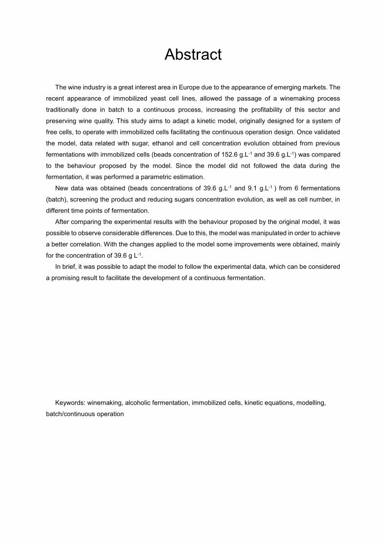
The wine industry is a great interest area in Europe due to the appearance of emerging markets. The
recent appearance of immobilized yeast cell lines, allowed the passage of a winemaking process
traditionally done in batch to a continuous process, increasing the profitability of this sector and
preserving wine quality. This study aims to adapt a kinetic model, originally designed for a system of
free cells, to operate with immobilized cells facilitating the continuous operation design. Once validated
the model, data related with sugar, ethanol and cell concentration evolution obtained from previous
fermentations with immobilized cells (beads concentration of 152.6 g.L-1 and 39.6 g.L-1) was compared
to the behaviour proposed by the model. Since the model did not followed the data during the
fermentation, it was performed a parametric estimation.
New data was obtained (beads concentrations of 39.6 g.L-1 and 9.1 g.L-1 ) from 6 fermentations
(batch), screening the product and reducing sugars concentration evolution, as well as cell number, in
different time points of fermentation.
After comparing the experimental results with the behaviour proposed by the original model, it was
possible to observe considerable differences. Due to this, the model was manipulated in order to achieve
a better correlation. With the changes applied to the model some improvements were obtained, mainly
for the concentration of 39.6 g L-1.
In brief, it was possible to adapt the model to follow the experimental data, which can be considered
a promising result to facilitate the development of a continuous fermentation.
Keywords: winemaking, alcoholic fermentation, immobilized cells, kinetic equations, modelling,
batch/continuous operation
i
Resumo
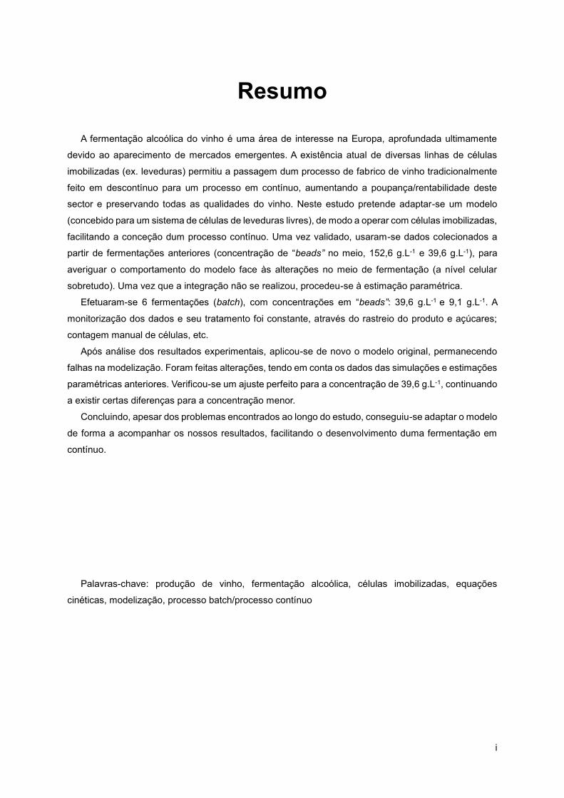
A fermentação alcoólica do vinho é uma área de interesse na Europa, aprofundada ultimamente
devido ao aparecimento de mercados emergentes. A existência atual de diversas linhas de células
imobilizadas (ex. leveduras) permitiu a passagem dum processo de fabrico de vinho tradicionalmente
feito em descontínuo para um processo em contínuo, aumentando a poupança/rentabilidade deste
sector e preservando todas as qualidades do vinho. Neste estudo pretende adaptar-se um modelo
(concebido para um sistema de células de leveduras livres), de modo a operar com células imobilizadas,
facilitando a conceção dum processo contínuo. Uma vez validado, usaram-se dados colecionados a
partir de fermentações anteriores (concentração de “beads” no meio, 152,6 g.L-1 e 39,6 g.L-1), para
averiguar o comportamento do modelo face às alterações no meio de fermentação (a nível celular
sobretudo). Uma vez que a integração não se realizou, procedeu-se à estimação paramétrica.
Efetuaram-se 6 fermentações (batch), com concentrações em “beads”: 39,6 g.L-1 e 9,1 g.L-1. A
monitorização dos dados e seu tratamento foi constante, através do rastreio do produto e açúcares;
contagem manual de células, etc.
Após análise dos resultados experimentais, aplicou-se de novo o modelo original, permanecendo
falhas na modelização. Foram feitas alterações, tendo em conta os dados das simulações e estimações
paramétricas anteriores. Verificou-se um ajuste perfeito para a concentração de 39,6 g.L-1, continuando
a existir certas diferenças para a concentração menor.
Concluindo, apesar dos problemas encontrados ao longo do estudo, conseguiu-se adaptar o modelo
de forma a acompanhar os nossos resultados, facilitando o desenvolvimento duma fermentação em
contínuo.
Palavras-chave: produção de vinho, fermentação alcoólica, células imobilizadas, equações
cinéticas, modelização, processo batch/processo contínuo
ii
Contents
Acknowledgments ................................................................................................................................. ii
Abstract ................................................................................................................................................. iii
Resumo.................................................................................................................................................... i
Contents ................................................................................................................................................. ii
List of Figures ....................................................................................................................................... iv
List of Tables ....................................................................................................................................... viii
List of Acronyms .................................................................................................................................. ix
1. Introduction .................................................................................................................................... 1
1.1. Winemaking ........................................................................................................................... 1
1.2. Alcoholic fermentation ........................................................................................................... 2
1.3. Malolactic fermentation .......................................................................................................... 4
1.4. Regulatory mechanisms ........................................................................................................ 4
1.5. Batch and continuous fermentation ....................................................................................... 5
1.6. Free and immobilized cells .................................................................................................... 6
1.7. Problem definition .................................................................................................................. 9
1.7.1. Models explanation ................................................................................................. 10
2. Aim of the work ............................................................................................................................ 16
3. Materials and Methods ................................................................................................................ 17
3.1. Preparation of fermentation ................................................................................................. 17
3.1.1. Fermentation medium ............................................................................................. 17
3.1.2. Immobilized yeasts ................................................................................................. 19
3.1.3. Yeast rehydration .................................................................................................... 19
3.1.4. Batch fermentation .................................................................................................. 20
3.2. Analytic methods ................................................................................................................. 20
3.2.1. CO2 determination .................................................................................................. 21
3.2.2. Biomass analysis .................................................................................................... 21
3.2.3. HPLC ...................................................................................................................... 23
3.2.4. DNS method ........................................................................................................... 24
3.2.5. Assimilable nitrogen determination ......................................................................... 26
3.3. Computational work ............................................................................................................. 27
4. Results and Discussion .............................................................................................................. 30
iii
4.1. Model validation with article results ..................................................................................... 30
4.2. Initial simulations with existing Data .................................................................................... 31
4.2.1. Presentation of experimental results ...................................................................... 31
4.2.2. Experimental Data simulation ................................................................................. 33
4.3. Simulations for the new experiments .................................................................................. 38
4.3.1. Presentation of new results .................................................................................... 38
4.3.2. Simulation with new Data (original parameters) ..................................................... 38
4.3.3. Simulation with new Data (new approach) ............................................................. 47
4.4. Reactor’s Modelling ............................................................................................................. 49
5. Conclusion and future perspectives ......................................................................................... 51
6. References .................................................................................................................................... 52
7. Annexes ........................................................................................................................................... I
iv
List of Figures
Figure 1.1 - Glycolytic pathway Embden-Meyerhof4 ............................................................................... 2
Figure 1.2- Metabolic pathway of ethanol fermentation in S.cerevisiae 9. Abbreviations : HK: hexokinase,
PGI: phosphoglucoisomerase, PFK: phosphofructokinase, FBPA: fructose bisphosphate aldolase, TPI:
triose phosphate isomerase, GAPDH: glyceraldehydes-3-phosphate dehydrogenase, PGK:
phosphoglycerate kinase, PGM: phosphoglyceromutase, ENO: enolase, PYK: pyruvate kinase, PDC:
pyruvate decarboxylase, ADH: alcohol dehydrogenase. ......................................................................... 3
Figure 1.3- Winemaking technology and immobilized cells3 ................................................................... 7
Figure 1.4-Immobilization techniques: A-attachment to a surface; B-the entrapment of cells in a porous
matrix gel; C-cell immobilization using barriers; D-flocculation. 3 ............................................................ 8
Figure 1.5- Simplified diagram describing the activity of a yeast31........................................................ 13
Figure 3.1 - Initial Medium “100% Grape Juice Carrefour Discount” .................................................... 17
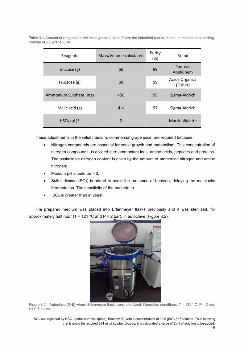
Figure 3.2 – Autoclave (SNI) where Erlenmeyer flasks were sterilized. Operation conditions: T = 121 °
C; P = 2 bar; t = 0.5 hours ..................................................................................................................... 18
Figure 3.3 - Package containing dry yeasts, S. cerevisiae strain var.bayanus, provided by Proenol Lda.
Analytical Characteristics: Solids > 86%; arsenic < 3 mg.kg-1; lead < 2 mg.kg-1; cadmium < 1 mg.kg-1;
mercury < 1 mg.kg-1; viable yeasts > 109 ufc.g-1; mesophilic aerobics bacteria < 103 ufc.g-1; mould < 103
ufc.g-1; coliforms < 103 ufc.g-1; E.coli is absent in 1 g (see also Annex II). ............................................ 19
Figure 3.4 - Incubated and Refrigerator Shaker, Thermo Scientifc MaxQ 400, used to achieve 20ºC
(isothermal condition) and an agitation of 100 rpm. .............................................................................. 20
Figure 3.5 – Laminar flow hood (Faster® KBN) used for sample's manipulation ................................. 21
Figure 3.6 - Instruments for Biomass Analysis: 1- The Optical microscope Leitz®, model Laborlux 12; 2-
Counting instrument: red button and white button pressed for every dead and living cell respectively. 22
Figure 3.7 - Thoma's cell filled with solution (50%(v/v) sample + 50%(v/v)methylene blue) used in the
measures throughout experiments ........................................................................................................ 22
Figure 3.8 - HPLC system ..................................................................................................................... 23
Figure 3.9 - Autosampler vials for HPLC, filled with the samples and standard solutions .................... 23
Figure 3.10 - DNS Reagent used for measurement of reducing sugars. .............................................. 24
Figure 3.11 - Calibration curve for glucose and the corresponding equation. ....................................... 25
Figure 3.12 - Material used for preparing the reaction of the samples with DNS reagent : 1-Eppendorfs
filled with 950 µL DNS reagent; 2- Fermentation samples; 3- “Special” pipette; 4- Beaker with DNS
reagent ( yellow ) ................................................................................................................................... 25

v
Figure 3.13 - Titration volumetric burette and its support, used for titration of the sample with the addition
of NaOH 0.1 M. ...................................................................................................................................... 26
Figure 3.14- Example of a simulation done on the fermentation study: Modelight program returns this
environment, where one can choose the initial concentrations, conditions and duration in which
fermentation takes place and the desired option for integration calculation. ........................................ 28
Figure 3.15 - Example of a parametric estimation done on the fermentation study: Modelight program
returns this environment, where one can choose the initial concentrations, conditions and duration in
which fermentation takes place and the desired option for integration calculation. The window returned
by the program also lets you select which parameters one wishes to fix / change and the ranges where
these can be calculated. ........................................................................................................................ 29
Figure 4.1 - Simulation of a fermentation with S0= 202 g.L-1, N0=0, 28 g.L-1 and a constant Temperature
T=24ºC (isothermal conditions). Comparison with the results obtained by article (Malherbe et al.
(2004)31). In this fermentation were used free yeast cells. .................................................................... 31
Figure 4.2 - Experimental results obtained by Kassim12 from a fermentation medium (such as shown in
3.1) .Constant Temperature (T) = 20 °C; S0 = 212 g.L-1; X0 (theory) = 3.81x10⁸ Cells.mL-1 (0.035 g.mL-1);
N0=0.161 g.L-1 ; Beads Concentration = 152.5 g .L-1. ........................................................................... 32
Figure 4.3 - Experimental results obtained by Kassim12 from a fermentation medium (such as shown in
3.1). Constant Temperature (T) = 20 °C; S0 = 205 g.L-1; X0 (theory) = 9.89x10⁷ Cells.mL-1 (0.008 g.mL-
1); N0=0.161 g.L-1 ; Beads Concentration = 39.6 g .L-1. ......................................................................... 32
Figure 4.5 - Simulations with estimated parameters (obtained by software Matlab and Excel) from
existing experimental data (Kassim, 2012)12, using the model developed by Malherbe et al. (2004)31.
Constant Temperature (T) = 20 °C; S0 = 205 g.L-1; X0 (theoric)= 9.89x10⁷ Cells.mL-1 (0.008 g.mL-1);
N0=0,161 g.L-1 ; Beads Concentration = 39.6 g .L-1. ............................................................................. 34
Figure 4.4 - Simulations with estimated parameters (obtained by software Matlab and Excel) from
existing experimental data (Kassim, 2012)12, using the model developed by Malherbe et al. (2004)31.
Constant Temperature (T) = 20 °C; S0 = 212 g.L-1; X0 (theory) = 3.81x10⁸ Cells.mL-1 (0.035 g.mL-1);
N0=0,161 g.L-1 ; Beads Concentration = 152.5 g.L-1. ............................................................................ 34
Figure 4.6 - Assays made for a bead concentration of 9.1 g.L-1. S0 =238.53 g.L-1(average); X0(theory) =
2.28x10⁷ cells.mL-1. Measurements were made for a fermentation time of 72.25 hours (t), and the control
of the same was determined by measurement using the DNS technique. ........................................... 38
Figure 4.7 - Assays made for a bead concentration of 39.6 g.L-1. S0 =223.54 g.L-1(average); X0(theory)
= 9.89x10⁷ cells.mL-1. Measurements were made for a fermentation time of 72.25 hours (t), and the
control of the same was determined by measurement using the DNS technique. ............................... 39
Figure 4.8 - Representation of the measured values (average of triplicates) related to cells (viables)
found in the medium, inside and outside of the beads, at a concentration of beds 39.6 g.L-1. The error
bars relate to statistical analysis (standard deviation). .......................................................................... 38
vi
Figure 4.9 - Representation of the measured values (average of triplicates) related to cells (viables)
found in the medium, inside and outside of the beads, at a concentration of beds 9.1 g.L-1. The error
bars relate to statistical analysis (standard deviation). .......................................................................... 38
Figure 4.10 - New experiments and simulation results made with the original model (original parameters)
for a bead concentration of 39.6 g.L-1 in the fermentation medium. Constant Temperature (T) = 20 °C;
S0 = 223.5 g.L-1 (average); X0 (real) = 5.76x10⁷ Cellules.mL-1 (1.05 g.L-1); N0=0.385 g.L-1. ................. 38
Figure 4.11 - New experiments and simulation results made with the original model (original parameters)
for a bead concentration of 9.1 g.L-1 in the fermentation medium. Constant Temperature (T) = 20 °C; S0
= 238.52 g.L-1; X0 (real)= 1.84x10⁷ Cellules.mL-1 (0.22 g.L-1); N0=0.385 g.L-1 . ..................................... 46
Figure 4.12 - New simulation results made with the adapted model for a bead concentration of 39.6 g.L-
1 in the fermentation medium. Constant Temperature (T) = 20 °C; S0 = 223.5 g.L-1 (average); X0 (real) =
5.76x10⁷ Cells.mL-1 (1.05 g.L-1); N0=0.421 g.L-1; ................................................................................... 48
Figure 4.13 - New simulation results made with the adapted model for a bead concentration of 9.1 g.L-1
in the fermentation medium. Constant Temperature (T) = 20 °C; S0 = 238.52 g.L-1(average); X0 (real)=
1.84x10⁷ Cells.mL-1 (0.22 g.L-1); N0=0.421 g.L-1 ; .................................................................................. 48
Figure 7.2 – Some information about immobilized yeast cells, ProRestart® (Proenol , Biotech Company)
.................................................................................................................................................................. I
Figure 7.3 - Calibration curve for ethanol and the corresponding equation. .......................................... II
Figure 7.4 - Calibration curve for glucose and the corresponding equation. .......................................... II
Figure 7.5 - Calibration curve for fructose and the corresponding equation. .......................................... II
Figure 7.6 - Representation of the measured values (average of triplicates) related to reducing sugars
present in the medium, at a concentration of beds 9.1 g.L-1. The error bars relate to statistical analysis
(standard deviation). ............................................................................................................................... III
Figure 7.7 - Representation of the measured values (average of triplicates) related to ethanol present in
the medium, at a concentration of beds 9.1 g.L-1. The error bars relate to statistical analysis (standard
deviation). ............................................................................................................................................... III
Figure 7.8 - Representation of the measured values (average of triplicates) related to CO2 released
during the fermentation, at a concentration of beds 9.1 g.L-1. The error bars relate to statistical analysis
(standard deviation). ............................................................................................................................... III
Figure 7.9 - Representation of the measured values (average of triplicates) related to reducing sugars
present in the medium, at a concentration of beds 39.6 g.L-1. The error bars relate to statistical analysis
(standard deviation). ............................................................................................................................... IV
Figure 7.10 - Representation of the measured values (average of triplicates) related to CO2 released
during the fermentation, at a concentration of beds 39.6 g.L-1. The error bars relate to statistical analysis
(standard deviation). ............................................................................................................................... IV

vii
Figure 7.11 - Representation of the measured values (average of triplicates) related to ethanol present
in the medium, at a concentration of beds 39.6 g.L-1. The error bars relate to statistical analysis (standard
deviation). ............................................................................................................................................... IV
Figure 7.12 – Relationship between the maximal fermentation rate, (dCO2/dt) max, and the assimilable
nitrogen concentration, Ninit. Graphic present in Colombié et al. (2005)48, for fermentations on synthetic
media at 24ºC.. ....................................................................................................................................... IV

viii
List of Tables
Table 1.1- Sugars and oxygen simultaneous effects in the metabolic regulation of the yeast
Saccharomyces cerevisiae12 ................................................................................................................... 5
Table 1.2 - Different models and their kinetic parameters for the representation of the alcoholic
fermentation33 34 ..................................................................................................................................... 10
Table 3.1-Amount of reagents to the initial grape juice to follow the industrial requirements, in relation to
a starting volume of 2 L grape juice. ...................................................................................................... 18
Table 4.1 - Conditions used in article’s simulation (Malherbe et al.(2004)31 ). ...................................... 30
Table 4.2 - Ranges used in many parameters estimation performed using Matlab and Excel. These
ranges were designed and created from several experiments where the model was tested in the limit
(differential equations), or from these values, the system failed to be resolve. .................................... 35
Table 4.3 - Calculated parameters in order to adjust the model to the experimental data. The original
parameters are presented (from the article Malherbe et al. (2004)31) and the calculated parameters
depending on the used programs for two bead concentrations. ........................................................... 38
Table 4.4 - Sugar measured by the DNS method (measuring the reducing sugars present in the
samples). Table Terminology: t01 respect to t = 0 of triplicate 1; t51 respect to t= 23.5 hours of triplicate
1; t81 respect to t = 46.5 hours of triplicate 1 and successively for all other triplicates (1,2,3 relate to the
beads at a concentration of 9.1 g.L-1; 4,5,6 relate to the concentration of 39.6 g.L-1) . ......................... 38
Table 4.5 - Average diameter (from triplicate) for the two concentrations tested. Values are given in mm
(millimetres). .......................................................................................................................................... 38
Table 4.6 - Representative dCO2/dt over 72.25 hours of fermentation for each one of tested
concentrations. In bold are indicated the (dCO2/dt)max . ........................................................................ 47
Table 4.7 - Simulation results in CSTR for a two stage reactor. Operating parameters such as Q, C0, Cf
were taken directly from Kassim12 study. The remaining parameters were calculated. As a reference for
the beads, it was admitted that 60.5 grams of dried beads were equivalent to a volume of 170 mL (when
rehydrated). tresid=(Cf-C0)/(rateconsum.sugars) .............................................................................................. 50
ix
List of Acronyms
ºC degree Celsius mm millimetre
µL microliter NAD nicotinamide adenine dinucleotide
ATP adenosine triphosphate PKF phosphofructokinase
C0 initial concentration Q flow
Cf final concentration tresid. residence time
D dilution rate ufc colony-forming unit
DNS dinitrosalicylic acid v volume
g grams w weight
GAP GTPase activating proteins
h hours
hL hectolitre
HPLC high-performance liquid chromatography
HXT hexose transporters
kg kilograms
L litre
min minutes
mL millilitre

1
1. Introduction
1.1. Winemaking
The process by which the wine is produced is called alcoholic fermentation. Fermentation processes
may be classified according: how the substrate is added and the production withdrawn. Thus, in a batch
fermentation, the substrate is added initially, and when it reaches the end of the fermentation, the product
is discharged out of the tank. The continuous operation involves successive addition of substrate to the
fermentation medium at the same rate at which the product is withdrawn. In semi-continuous and fed-
batch process the substrate is added and the product withdrawn at timed intervals, and these form the
product has characteristics of both types1.
In the last few years, the French winery industry as the European one, has suffered competition from
new emerging economies2. To struggle this, the investigation of new oenological techniques has risen
in France and in the rest of European Union.
In winemaking, the continuous fermentation system should be capable of respond to a major problem
that is the inhibitory effect of the products formed during the growth of the microorganisms. However,
when immobilized cells are used, this problem is softened as immobilized cells are more tolerant to
inhibitory end products such as ethanol.
The development of new technics including heat treatment tools for optimal extraction of colour and
polyphenols by continuous processes, greatly contributes to standardized wine production. Among
these techniques, the continuous fermentations also enable better control and a homogenization of the
organoleptic quality of the products. In addition to an expected reduction in fermentation time, this
process would remove all production downtime (time winery, racking, cleaning), which also contribute
to the increase of productivity. However there are some problems associated with the implementation
of a continuous system in wine making to maintain aseptic system for long periods of time (at least
several weeks). If a system is contaminated and there is a need to stop the process, one has to make
a new immobilization, increasing process costs and reducing production. In order to avoid contamination
in both operation modes, it is used high concentrations of SO2 3 .
Wine production units are continually undergoing modernization. Improvements are particularly
important for the fermentation step, which, despite being a major part of the wine production process, is
still carried out empirically. If this step could be made more efficiently, the management of tanks and
energy will be improved. Indeed, prediction and optimization of the duration of the fermentation and
minimization of the energy required to cool one tank, or the entire winery, are currently major challenges
for oenologists.
2
1.2. Alcoholic fermentation
Alcoholic fermentation is the biological transformation of grape sugars (primarily glucose and
fructose) in ethanol and carbon dioxide, according to the Equation (1). This production of alcohol is
accompanied by the formation of by products such as glycerol, acetic acid, lactic acid, alcohols and
esters.
𝐶6𝐻12𝑂6 → 2𝐶2𝐻5𝑂𝐻 + 2𝐶𝑂2 (1)
During alcoholic fermentation, the sugars contained in the grape are converted into alcohol by a
series of complex reactions. Glycolysis, process common to fermentation and respiration, is the starting
point, in which glucose is converted into pyruvic acid. In fermentation conditions, pyruvic acid is
decarboxylase into acetaldehyde, which is itself reduced to ethanol. In the case of respiration, pyruvic
acid enters on the citric acid cycle to be oxidized into CO2 and H2O4.
The fermentation is generally conducted by yeasts of the specie Saccharomyces cerevisiae.
Although these are slightly present on the grapes (2-3% relating to all microorganisms present )5, during
fermentation they become the majority and thus constitute the principal motor of the fermentation.
Normally, at 30°C, the anaerobic ethanol production rate is close to 30 mmol.biomass-1.h-1 6 .
S. cerevisiae, yeast commonly used in the wine industry, contains a complex system for the transport
of hexoses. The 32 members of the family HXT (hexose transporters) have different functions with
respect to regulation of transcription, substrate specificity and affinity for glucose, as there are other
sources 7.
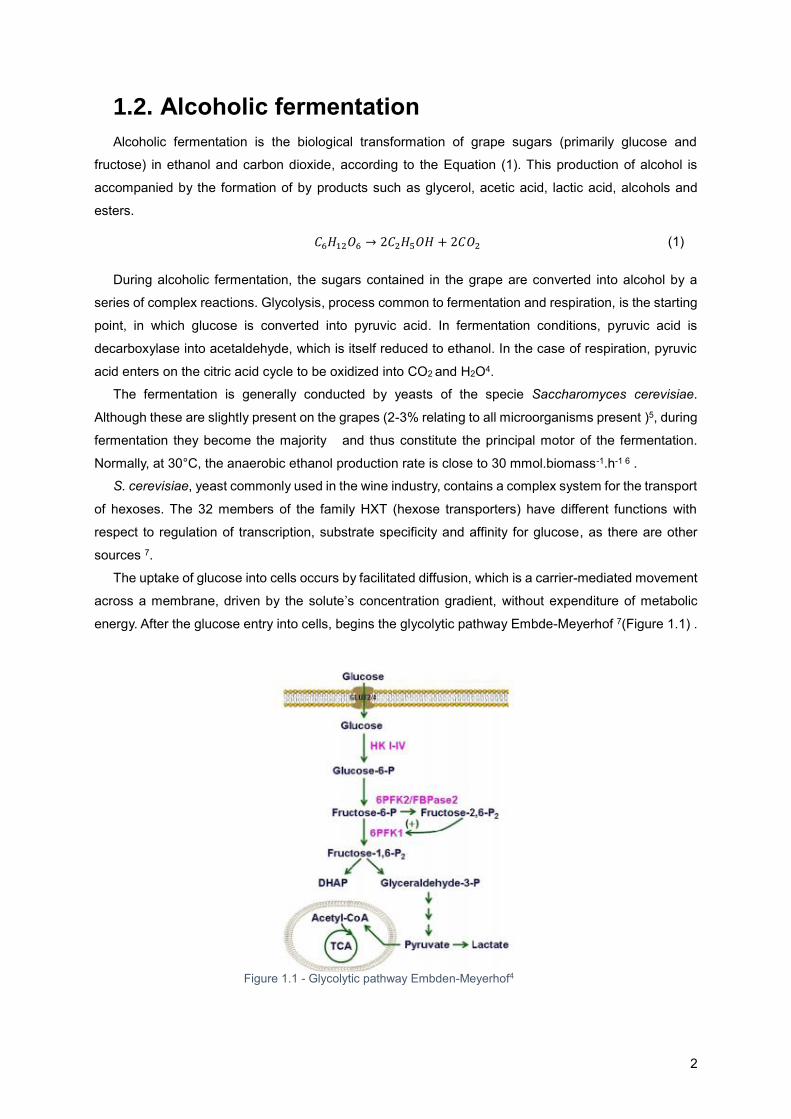
The uptake of glucose into cells occurs by facilitated diffusion, which is a carrier-mediated movement
across a membrane, driven by the solute’s concentration gradient, without expenditure of metabolic
energy. After the glucose entry into cells, begins the glycolytic pathway Embde-Meyerhof 7(Figure 1.1) .
Figure 1.1 - Glycolytic pathway Embden-Meyerhof4
3
This metabolic pathway is composed of glycolysis, then the decarboxylation of pyruvic acid reduction.
During glycolysis, glucose molecule begins by being split into two triose phosphate molecules. This first
step (energy consuming) involves two phosphorylation reactions and isomerization reaction.
Subsequently, the molecule of triose phosphate is converted to pyruvate for energy recovery in the form
of ATP molecules of NADH formation. Pyruvate then undergoes a decarboxylation, leading to
acetaldehyde which will itself be reduced to ethanol. At the same time, it is possible to see the
regeneration of the carrier; NADH+ takes its oxidized form of NAD+. However, if acetaldehyde doesn’t
exist, another electron acceptor can be considered: dihydroxyacetone phosphate isomer of GAP
(glyceraldehyde 3-phosphate). The reduction of this ketone leads to glycerol. So as evidenced, two
electron acceptors can be considered, however acetaldehyde has better affinity for a common carrier,
which mean that the flux towards the production of ethanol will be greater. In addition, to a certain
concentration of ethanol, feedback inhibition is set up at the dihydroxyacetone reduction enzyme,
slowing, blocking in this way the synthesis of glycerol. The synthesis of ethanol, in turn, continues until
reached a high level, inducing a feedback inhibition effect on glucose transporters and fructose as well
as ensuring hexokinase phosphorylation of glucose. Thus the fermentation stops, leaving in the middle
unassimilated sugars. Alcohol levels which feedback inhibitions occurs vary depending on the strain and
the environmental conditions. In general, slower glycerol synthesis is about 4 to 5% (v/v) ethanol and a
complete inhibition of the consumptions of sugars generally takes place around 13 to 15% (v/v) 8.
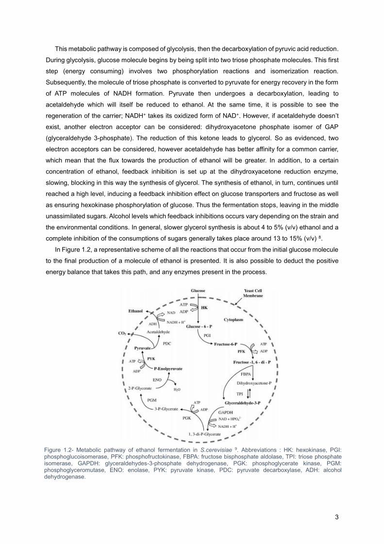
In Figure 1.2, a representative scheme of all the reactions that occur from the initial glucose molecule
to the final production of a molecule of ethanol is presented. It is also possible to deduct the positive
energy balance that takes this path, and any enzymes present in the process.
Figure 1.2- Metabolic pathway of ethanol fermentation in S.cerevisiae 9. Abbreviations : HK: hexokinase, PGI: phosphoglucoisomerase, PFK: phosphofructokinase, FBPA: fructose bisphosphate aldolase, TPI: triose phosphate isomerase, GAPDH: glyceraldehydes-3-phosphate dehydrogenase, PGK: phosphoglycerate kinase, PGM: phosphoglyceromutase, ENO: enolase, PYK: pyruvate kinase, PDC: pyruvate decarboxylase, ADH: alcohol dehydrogenase.
4
In this pathway there are two pyruvate molecules produced from one molecule of glucose. Under
anaerobic conditions the ethanol is produced, accompanied by the release of CO2 as mentioned above.
Theoretically, the yields are 0.511 and 0.489 respectively for ethanol and CO2, using as a reference a
mass basis of assimilable glucose 9. The final balance of two ATPs produced in the process is used for
biosynthesis of yeast cells that require a lot of energy, i.e., ethanol production is accompanied by a
cellular growth. If these ATPs are not consumed, the cell growth opening, since the glycolysis metabolic
pathway is interrupted due to the action of PFK kinase, which is activated by intracellular accumulation
of ATP9.
1.3. Malolactic fermentation
Specifically, the winemaking process (nearly all red wines and many white wines) includes other main
step beyond alcoholic fermentation called malolactic fermentation. One of the main effects of the
malolactic fermentation is deacidification, which is particularly desirable for high acid wine produced in
cool climate regions, such as New Zealand and the United Kingdom. Malolactic fermentation is often
spontaneous and difficult to stop in red winemaking, possibly due to the higher temperatures involved
and/or through the activities of indigenous lactic bacteria found in cooperage. Producers will allow it to
proceed or actively encourage it early in the life of a wine in order to prevent it happening in the bottle.
Normally, it is conducted by acid bacteria, following the alcoholic fermentation explained above. These
microorganisms (including yeasts) grow in the grapes, but yeasts are more willing to grow than lactic
acid bacteria, so the alcoholic fermentation starts quicker. There are various lactic acid bacteria species
(today are known ten species present in grapes, as Oenococcus oeni). Acetic acid bacteria can survive
in low concentrations, due to the low redox potential of the medium as soon as grapes are poured into
fermentation tanks. When all reducing sugars are fermented to ethanol, yeast levels decline and lactic
acid bacteria growth occurs. The term malolactic fermentation however is not correct since the
transformation of L-malic acid to L-lactic acid is not a fermentative pathway, but a decarboxylation
(Equation (2)). Once all malic acid is degraded, lactic acid bacteria are eliminated by sulphites. Sulphur
dioxide is at this stage of winemaking the only authorized and efficient agent for the microbial
stabilization of wine. Nearly all red wines and many white wines are obtained by these two fermentation
steps 10.
𝐶4𝐻6𝑂5 → 𝐶3𝐻6𝑂3 + 𝐶𝑂2 (2)
1.4. Regulatory mechanisms
The activation of specific metabolic pathways for desired product production, in this case the wine,
depends on genetics mechanisms on the cell and certain external factors such as pH, temperature,
presence of inhibitors compounds or the initial medium composition or substrate.
Normally, switching between respiration and fermentation is a microorganism cell response to
concentrations of sugars and oxygen, i.e. the Crabtree effect and the Pasteur effect 11. The Crabtree
effect translates briefly the catabolic repression mechanism of the respiratory chain by glucose. As in
the production of wines with low oxygen content conditions, the common organism used is the yeast
5
Saccharomyces cerevisiae (Crabtree positive) and the substrates are heavily concentrated in sugar
production, the response is directed to the synthesis of ethanol. Pasteur effect, briefly, means the
switching between fermentation and respiration, due to the action and presence / absence of oxygen.
In the Table 1.1 are shown the combined effects, depending on the conditions, the sugar and oxygen in
the metabolic regulation of this yeast.
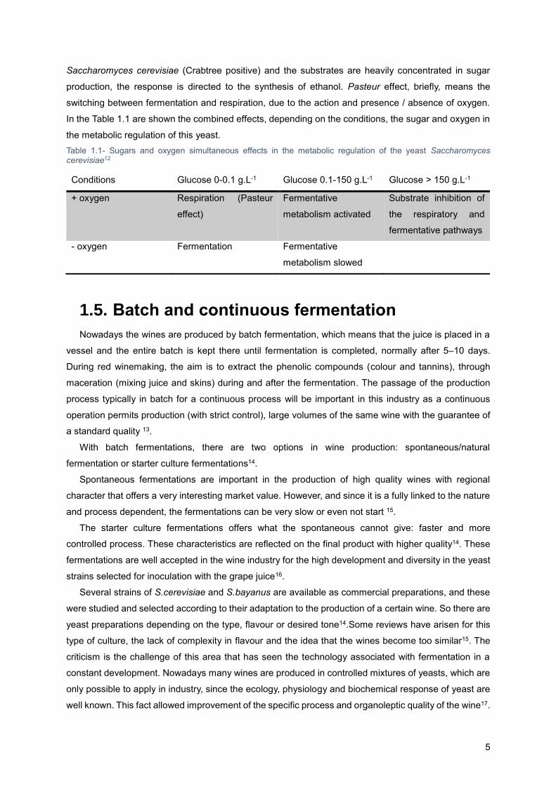
Table 1.1- Sugars and oxygen simultaneous effects in the metabolic regulation of the yeast Saccharomyces cerevisiae12
Conditions Glucose 0-0.1 g.L-1 Glucose 0.1-150 g.L-1 Glucose > 150 g.L-1
+ oxygen Respiration (Pasteur
effect)
Fermentative
metabolism activated
Substrate inhibition of
the respiratory and
fermentative pathways
- oxygen Fermentation Fermentative
metabolism slowed
1.5. Batch and continuous fermentation
Nowadays the wines are produced by batch fermentation, which means that the juice is placed in a
vessel and the entire batch is kept there until fermentation is completed, normally after 5–10 days.
During red winemaking, the aim is to extract the phenolic compounds (colour and tannins), through
maceration (mixing juice and skins) during and after the fermentation. The passage of the production
process typically in batch for a continuous process will be important in this industry as a continuous
operation permits production (with strict control), large volumes of the same wine with the guarantee of
a standard quality 13.
With batch fermentations, there are two options in wine production: spontaneous/natural
fermentation or starter culture fermentations14.
Spontaneous fermentations are important in the production of high quality wines with regional
character that offers a very interesting market value. However, and since it is a fully linked to the nature
and process dependent, the fermentations can be very slow or even not start 15.
The starter culture fermentations offers what the spontaneous cannot give: faster and more
controlled process. These characteristics are reflected on the final product with higher quality14. These
fermentations are well accepted in the wine industry for the high development and diversity in the yeast
strains selected for inoculation with the grape juice16.
Several strains of S.cerevisiae and S.bayanus are available as commercial preparations, and these
were studied and selected according to their adaptation to the production of a certain wine. So there are
yeast preparations depending on the type, flavour or desired tone14.Some reviews have arisen for this
type of culture, the lack of complexity in flavour and the idea that the wines become too similar15. The
criticism is the challenge of this area that has seen the technology associated with fermentation in a
constant development. Nowadays many wines are produced in controlled mixtures of yeasts, which are
only possible to apply in industry, since the ecology, physiology and biochemical response of yeast are
well known. This fact allowed improvement of the specific process and organoleptic quality of the wine17.

6
In a batch process, the fermentation takes place in a tank where it is placed grape juice, keeping this
space until fermentation end. In modern wineries are used cylindrical-conical vessel made of stainless
steel. For many years, the systematic ability to control these tanks (temperature, aeration and agitation),
made possible the use of this technology easily and successfully18.
However, batch fermentations have inherent inefficiencies, such as the low speed of the process and
the dependency on the growth of cell populations 17.
Besides that, it is also possible to refer other disadvantages associated with a batch process, such
as: before starting a new batch fermentation, it is expected that the previous batch is complete and is
removed from the vessel (downtime). For all these reasons, high costs are associated due to the large
volumes of fermenters. In the downstream process, the microbial cells must be separated from the
product, decreasing the yield.
As mentioned above, various technologies and innovations have been implemented in the
fermentation process. Some innovations are connected to a high cell density (of 109-1010 cells.mL-1)
which can now be applied to fermentation by accelerating the biochemical reactions such as the
transformation of the sugar alcohol to values of order of 10 to 100 more rapidly than those occurring in
the batch process 19;20.
Nowadays, there are several bioreactors developed for continuous operation. For example, the
membrane reactor, where the reactions are continuously occurring with greater efficiency, because high
cell densities are reached. Its application, among other models of continuous reactors are referenced in
Verbelen et al. (2006) 20 .
Experiments at laboratory level have shown that the enormous potential of bioreactors technologies
can bring in the winemaking. However, the scale-up to pilot or industrial scale, usually presents a number
of challenges that require further study and knowledge. Working with medium with enough particles can
cause blockages in column reactors or impossible contact with the membranes in the case of a reactor
of this type, interrupting the process which is expensive. Existing yeast or bacteria in the environment
can also accumulate over time in the reactor which impedes their good performance.
Another important factor in a continuous process, is the possible reaction instability of the yeast cells
in the reactor due to the huge physical, chemical and biological stress in continuous reactors. Carbon
dioxide is a product of fermentation that can also be another factor to consider on continuous
processes13;9.Another relevant aspect is the transport of cultures accustomed to a batch process into a
continuous process. The behaviour of cells at the level of their metabolism can be modified due to
changing operating conditions, which is reflected in a different organoleptic profile to level the final
product. Then, a continuous process to be effective, in principle, a wide study selection of techniques
and methods needs to be performed, at the level of the yeasts17.
1.6. Free and immobilized cells
Normally, wine industries use free cells. In more recent years, new technologies have been
investigated and implemented to improve the biological processes. However the continuous process
always found some problems on an industrial scale due to the enormous risks that it involves (maintain

7
product quality over time). The major step of turning was given with the appearance of immobilized cells
on the market, which allows to obtain a standard product with greater safety 22.
The concept of immobilized cells was proposed in the 1970s23 and it was initially developed from the
concept of enzyme immobilization, designed to simplify certain bioreactions that occurred with the
presence of numerous enzymes involved cofactors. In the beginning there was a suspicion with this new
industry paradigm. Although all the implicit economic advantages (such as ease of separation of the
medium and reuse), the fact of using synthetic materials meant that the cells have a new environment
and may not work efficiently.
Recently, research has been done in this area to develop immobilization techniques and to choose
materials to improve this fermentation. In the related alcoholic fermentation industry, the main purpose
of using immobilized cells is productivity increase, reducing the necessary fermenter’s volume 9.
An important factor, and since it deals with the immobilization of cells in a food industry, identification
of the support and its food grade purity must be written13. The support should be abundant in nature,
low cost and must not interfere with the sensory characteristics of the final product13. In the winemaking
process, as can be seen in Figure 1.3, the immobilized cell system can be used in in the alcoholic,
malolactic and malo-alcoholic fermentations.
Theoretically, the immobilized cells would be advantageous in production of secondary metabolites,
comparing with primary metabolites which are highly related to cell growth. When cells are immobilized,
their growth is affected by various factors such as physical limitations (mass transfer), access to nutrients
present in the medium and accumulation of toxic agents, due to the limitations on mass transfer9.
As in the case of a fermentation, which is the work object, ethanol is the product of interest being a
primary metabolite, the use of immobilized cells must be thoroughly studied. Ethanol production is
related to cell growth. As already mentioned, if there is ATP accumulation due to the disparity between
the rate of ethanol production and cell growth, is activated an enzyme which interrupts glycolysis,
affecting the process. Due to this fact, the research in the area of inert materials has been developed in
recent decades to facilitate cell growth9.However, there are some rewards of immobilization of the cells
and their physical constriction. Because the cells are aggregated and very close (metabolism can
change), yeasts have more protection against the inhibitory ethanol. An experiment conducted by Jirku
(1999)24, demonstrated that the leakage of UV-absorbing intracellular substance was greatly reduced in
the immobilized cells, compared with that of free yeast cells in the same medium. Other studies reveal
Figure 1.3- Winemaking technology and immobilized cells3
8
that the specific death rate for the gel immobilized yeast cells decreases to one tenth compared with the
free yeast cells, when they were placed in ethanol 50% (v / v) for 15 hours25.
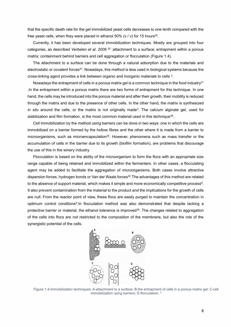
Currently, it has been developed several immobilization techniques. Mostly are grouped into four
categories, as described Verbelen et al. 2006 20 :attachment to a surface; entrapment within a porous
matrix; containment behind barriers and cell aggregation or flocculation (Figure 1.4).
The attachment to a surface can be done through a natural adsorption due to the materials and
electrostatic or covalent forces27. Nowadays, this method is less used in biological systems because the
cross-linking agent provides a link between organic and inorganic materials to cells 3.
Nowadays the entrapment of cells in a porous matrix gel is a common technique in the food industry21
.In the entrapment within a porous matrix there are two forms of entrapment for this technique. In one
hand, the cells may be introduced into the porous material and after their growth, their mobility is reduced
through the matrix and due to the presence of other cells. In the other hand, the matrix is synthesized
in situ around the cells, or the matrix is not originally made3. The calcium alginate gel, used for
stabilization and film formation, is the most common material used in this technique28.
Cell immobilization by the method using barriers can be done in two ways: one in which the cells are
immobilized on a barrier formed by the hollow fibres and the other where it is made from a barrier to
microorganisms, such as microencapsulation20. However, phenomena such as mass transfer or the
accumulation of cells in the barrier due to its growth (biofilm formation), are problems that discourage
the use of this in the winery industry.
Flocculation is based on the ability of the microorganism to form the flocs with an appropriate size
range capable of being retained and immobilized within the fermenters. In other cases, a flocculating
agent may be added to facilitate the aggregation of microorganisms. Both cases involve attractive
dispersion forces, hydrogen bonds or Van der Waals forces20.The advantages of this method are related
to the absence of support material, which makes it simple and more economically competitive process9.
It also prevent contamination from the material to the product and the implications for the growth of cells
are null. From the reactor point of view, these flocs are easily purged to maintain the concentration in
optimum control conditions9.In flocculation method was also demonstrated that despite lacking a
protective barrier or material, the ethanol tolerance is improved29. The changes related to aggregation
of the cells into flocs are not restricted to the composition of the membrane, but also the role of the
synergistic potential of the cells.
Figure 1.4-Immobilization techniques: A-attachment to a surface; B-the entrapment of cells in a porous matrix gel; C-cell immobilization using barriers; D-flocculation. 3
9
1.7. Problem definition
Over the past fifteen years, numerous research models describing the kinetics behaviour of alcoholic
fermentation30 have been published. The majority of the models are “knowledge-based” (deterministic)
models which take into consideration main phenomena that affect the kinetics of alcoholic fermentation.
There are other models resulting from the macroscopic analysis of the alcoholic fermentation process
that require the estimation of fewer parameters, although their physiological significance is difficult to
interpret31.
Another approach to the modelling problem consists in the elaboration of data driven model. In this
model, the explicit variables at a specific level of prediction are a function of the values of the descriptive
variables at the present and preceding moments. Some of the models are of “the black box” type and
use neural networks32. These give useful information on the development of the fermentation process
based on data from the beginning of the process. Finally, there are other empirical models, in which the
form of the equations is based only on their aptitude to describe the experimental data32.
Although there are many models in the field of ethanol production at an industrial scale, the interest
is centred on models applicable to oenology. Many models of biological reactions are based on mass
conservation. However, alcoholic fermentation in oenological conditions must be dealt differently.
One of the problems in the preparation of a realistic model for fermentation, as stated above, is the
inhibitory effect in cell growth due to ethanol and also for the production of ethanol, as inhibits glycolysis9.
Several models have been developed in recent years, in an attempt to find a close approach of what
goes on the biological level.
The ideal model for a winemaker should be able to predict the kinetic behaviour of the fermentation
process based on the initial characteristics of grape juice. Stablish an alcoholic fermentation model
provides a useful tool to plan and study the implementation of a new process, bringing also several
economic advantages. The ability to accurately estimate the duration of the fermentation process (time
when the sugar is exhausted), allows an efficient utilization of existent resources in a factory. The
prediction of CO2 production rate becomes important to control the level of the aromatic quality of wines.
The energy levels implications have to be taken into account, as well, since the process kinetics
knowledge allows the calculation the levels of heat generated during fermentation by knowing the
heating peak of the process and therefore it acts rationally within the cooling32.
Some fermentation models are presented in the following section, especially the target model of this
work, described here as a mathematical construction that can be used in a wide range of oenological
conditions31. The model presented herein is based on physiological considerations and takes into
account the main phenomena that directly affect the kinetics in these specific conditions, such as:
nitrogen in yeast synthesis (growth phase) and the activation of metabolism (stationary phase); the
transport of sugar into yeast cells; ethanol inhibition; and temperature, including anisothermal
conditions, which is known to be very common in wine-making31.
10
1.7.1. Models explanation
Generally, the models used to describe the kinetics of fermentation are represented by the following
differential equations (Equations (3)(4)(5)) 33:
𝑑𝑋
𝑑𝑡= 𝜇𝑋
(3)
𝑑𝑃
𝑑𝑡= 𝑞𝑋
(4)
𝑑𝑆
𝑑𝑡= − (
1
𝑌𝑥/𝑠 𝑑𝑋
𝑑𝑡 ) − (
1
𝑌𝑝/𝑠 𝑑𝑃
𝑑𝑡)
(5)
where X, P and S are respectively the biomass, product and substrate concentration (g.L-1); μ and q are
the specific growth rates respectively of biomass and product; Yx/s is the biomass yield over the substrate
consumption (g.g-1) and Yp/s is the product yield over the substrate consumption (g.g-1).
The equations presented above are usually the basis of the kinetic description of the alcoholic
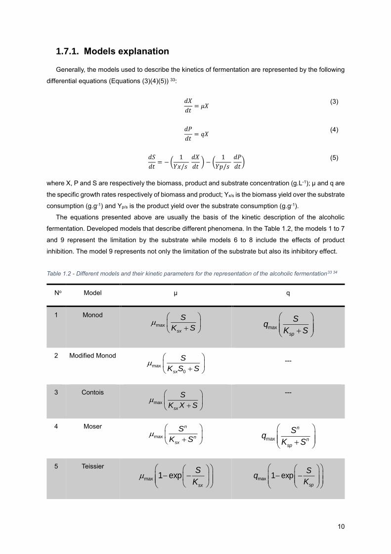
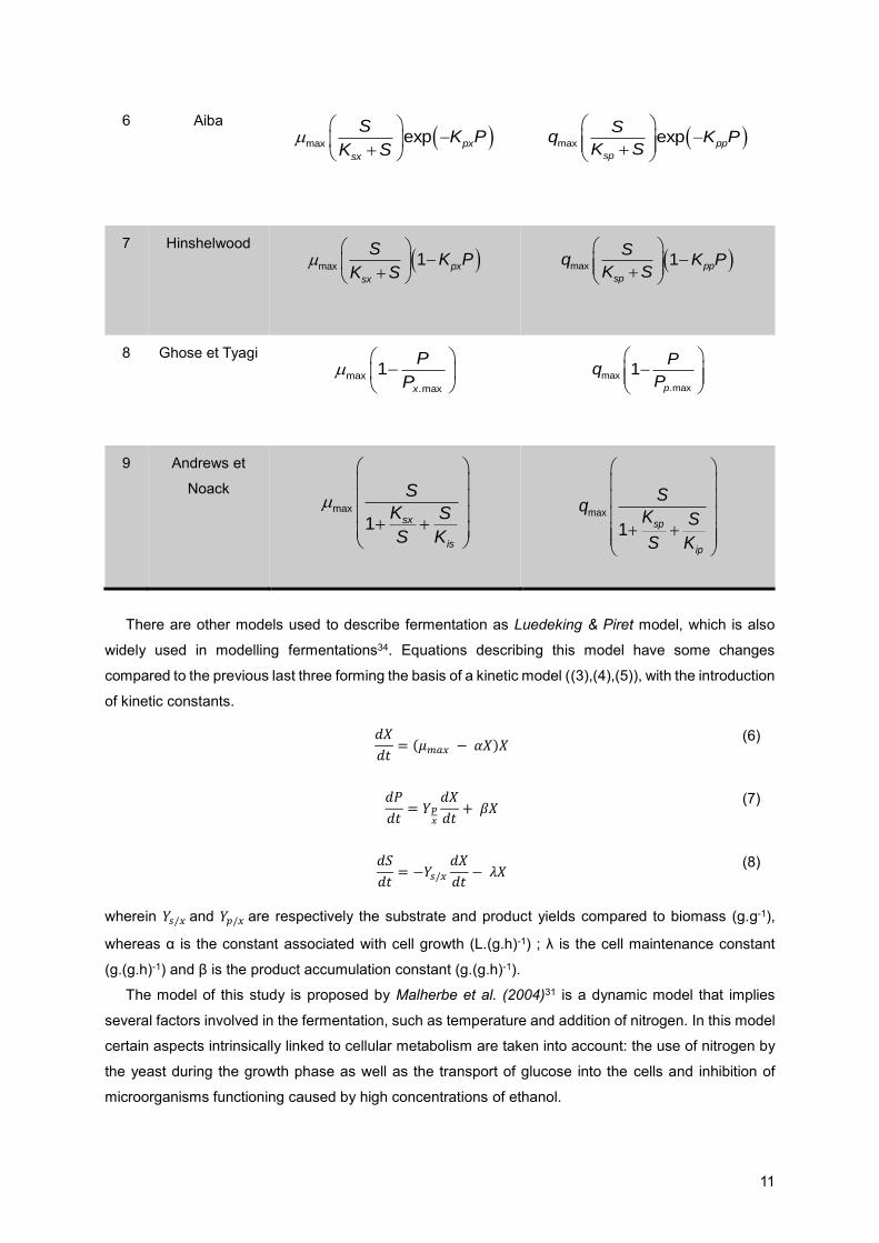
fermentation. Developed models that describe different phenomena. In the Table 1.2, the models 1 to 7
and 9 represent the limitation by the substrate while models 6 to 8 include the effects of product
inhibition. The model 9 represents not only the limitation of the substrate but also its inhibitory effect.
Table 1.2 - Different models and their kinetic parameters for the representation of the alcoholic fermentation33 34
No Model µ q
1 Monod
max
sx
S
K S
max
sp
Sq
K S
2 Modified Monod
max
0sx
S
K S S
---
3 Contois
max
sx
S
K X S
---
4 Moser
max
n
n
sx
S
K S
max
n
n
sp
Sq
K S
5 Teissier
max 1 expsx
S
K
max 1 expsp
Sq
K
11
6 Aiba
max exp px
sx
SK P
K S
max exp pp
sp
Sq K P
K S
7 Hinshelwood
max 1 px
sx
SK P
K S
max 1 pp
sp
Sq K P
K S
8 Ghose et Tyagi
max
.max
1x
P
P
max
.max
1p
Pq
P
9 Andrews et
Noack
max
1 sx
is
S
K S
S K
max
1 sp
ip
Sq
K S
S K
There are other models used to describe fermentation as Luedeking & Piret model, which is also
widely used in modelling fermentations34. Equations describing this model have some changes
compared to the previous last three forming the basis of a kinetic model ((3),(4),(5)), with the introduction
of kinetic constants.
𝑑𝑋
𝑑𝑡= (𝜇𝑚𝑎𝑥 − 𝛼𝑋)𝑋
(6)
𝑑𝑃
𝑑𝑡= 𝑌𝑝
𝑥
𝑑𝑋
𝑑𝑡+ 𝛽𝑋
(7)
𝑑𝑆
𝑑𝑡= −𝑌𝑠/𝑥
𝑑𝑋
𝑑𝑡− 𝜆𝑋
(8)
wherein 𝑌𝑠/𝑥 and 𝑌𝑝/𝑥 are respectively the substrate and product yields compared to biomass (g.g-1),
whereas α is the constant associated with cell growth (L.(g.h)-1) ; λ is the cell maintenance constant
(g.(g.h)-1) and β is the product accumulation constant (g.(g.h)-1).
The model of this study is proposed by Malherbe et al. (2004)31 is a dynamic model that implies
several factors involved in the fermentation, such as temperature and addition of nitrogen. In this model
certain aspects intrinsically linked to cellular metabolism are taken into account: the use of nitrogen by
the yeast during the growth phase as well as the transport of glucose into the cells and inhibition of
microorganisms functioning caused by high concentrations of ethanol.
12
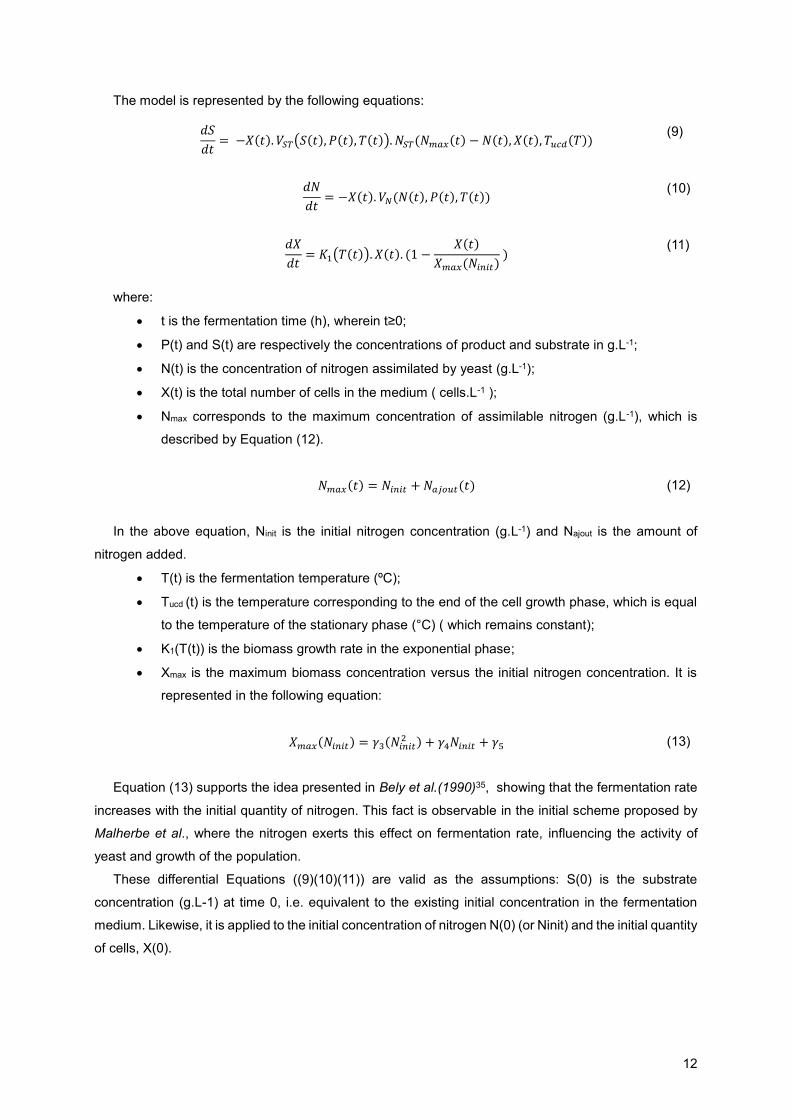
The model is represented by the following equations:
𝑑𝑆
𝑑𝑡= −𝑋(𝑡). 𝑉𝑆𝑇(𝑆(𝑡), 𝑃(𝑡), 𝑇(𝑡)). 𝑁𝑆𝑇(𝑁𝑚𝑎𝑥(𝑡) − 𝑁(𝑡), 𝑋(𝑡), 𝑇𝑢𝑐𝑑(𝑇))
(9)
𝑑𝑁
𝑑𝑡= −𝑋(𝑡). 𝑉𝑁(𝑁(𝑡), 𝑃(𝑡), 𝑇(𝑡))
(10)
𝑑𝑋
𝑑𝑡= 𝐾1(𝑇(𝑡)). 𝑋(𝑡). (1 −
𝑋(𝑡)
𝑋𝑚𝑎𝑥(𝑁𝑖𝑛𝑖𝑡) )
(11)
where:
t is the fermentation time (h), wherein t≥0;
P(t) and S(t) are respectively the concentrations of product and substrate in g.L-1;
N(t) is the concentration of nitrogen assimilated by yeast (g.L-1);
X(t) is the total number of cells in the medium ( cells.L-1 );
Nmax corresponds to the maximum concentration of assimilable nitrogen (g.L-1), which is
described by Equation (12).
𝑁𝑚𝑎𝑥(𝑡) = 𝑁𝑖𝑛𝑖𝑡 + 𝑁𝑎𝑗𝑜𝑢𝑡(𝑡) (12)
In the above equation, Ninit is the initial nitrogen concentration (g.L-1) and Najout is the amount of
nitrogen added.
T(t) is the fermentation temperature (ºC);
Tucd (t) is the temperature corresponding to the end of the cell growth phase, which is equal
to the temperature of the stationary phase (°C) ( which remains constant);
K1(T(t)) is the biomass growth rate in the exponential phase;
Xmax is the maximum biomass concentration versus the initial nitrogen concentration. It is
represented in the following equation:
𝑋𝑚𝑎𝑥(𝑁𝑖𝑛𝑖𝑡) = 𝛾3(𝑁𝑖𝑛𝑖𝑡2 ) + 𝛾4𝑁𝑖𝑛𝑖𝑡 + 𝛾5 (13)
Equation (13) supports the idea presented in Bely et al.(1990)35, showing that the fermentation rate
increases with the initial quantity of nitrogen. This fact is observable in the initial scheme proposed by
Malherbe et al., where the nitrogen exerts this effect on fermentation rate, influencing the activity of
yeast and growth of the population.
These differential Equations ((9)(10)(11)) are valid as the assumptions: S(0) is the substrate
concentration (g.L-1) at time 0, i.e. equivalent to the existing initial concentration in the fermentation
medium. Likewise, it is applied to the initial concentration of nitrogen N(0) (or Ninit) and the initial quantity
of cells, X(0).

13
In relation to the activity of the yeast, the models considers 4 phenomena: in glycolysis, glucose
transport, nitrogen transport and synthesis of glucose transporters. The following diagram illustrates this
fact (Figure 1.5):
The transport of glucose depends first on glucose concentration but also on the concentration of
ethanol present in the fermentation medium (can be inhibitory), and it is present in the scheme proposed
by the authors. The facilitated diffusion mechanism is described by the following equation:
𝜈𝑆𝑇(𝑆, 𝐸, 𝑇) =
𝐾2(𝑇)𝑆
𝑆 + 𝐾𝑆 + 𝐾𝑆𝐼𝑆𝐸𝛼𝑆
(14)
where
KS is the affinity constant of sugar transporters (g.L-1);
KSI is the constant for the inhibition of sugar transporters by ethanol (L.g-1);
E is the product, ethanol (g.L-1);
αS is other constant;
K2 (T) is a function depending on temperature. Overall this equation describes the active
transport of glucose per transporter (g.h-1).
The quantification of the number of transporters in a yeast is represented by 𝑁𝑆𝑇 (Equation (15)).
This expression simplifies the way of how a cell transforms nitrogen molecules into glucose transporters.
The function thus depends on the amount of absorbed nitrogen and the conditions (temperature T),
related with the mechanism. In isothermal conditions, the author proposed a model represented by
Equation (15) :
Figure 1.5- Simplified diagram describing the activity of a yeast31
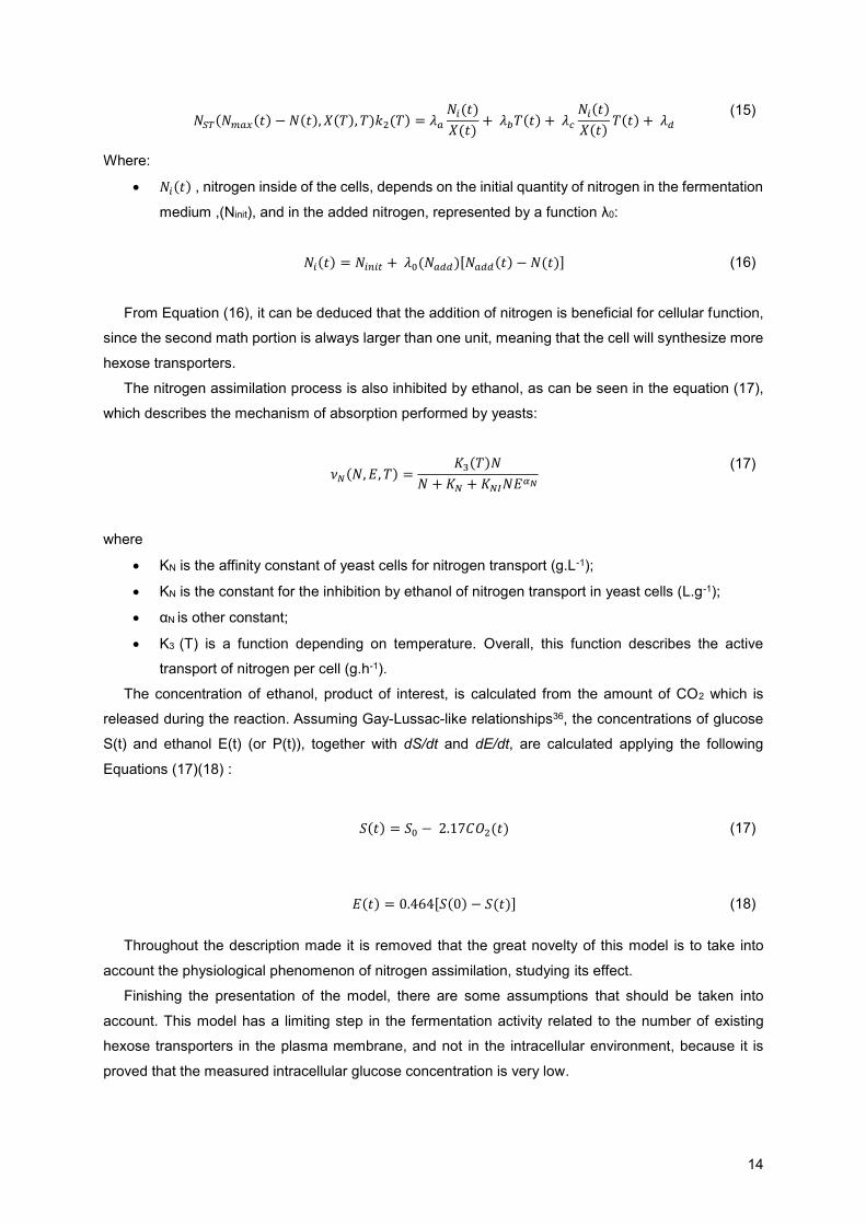
14
𝑁𝑆𝑇(𝑁𝑚𝑎𝑥(𝑡) − 𝑁(𝑡), 𝑋(𝑇), 𝑇)𝑘2(𝑇) = 𝜆𝑎
𝑁𝑖(𝑡)
𝑋(𝑡)+ 𝜆𝑏𝑇(𝑡) + 𝜆𝑐
𝑁𝑖(𝑡)
𝑋(𝑡)𝑇(𝑡) + 𝜆𝑑
(15)
Where:
𝑁𝑖(𝑡) , nitrogen inside of the cells, depends on the initial quantity of nitrogen in the fermentation
medium ,(Ninit), and in the added nitrogen, represented by a function λ0:
𝑁𝑖(𝑡) = 𝑁𝑖𝑛𝑖𝑡 + 𝜆0(𝑁𝑎𝑑𝑑)[𝑁𝑎𝑑𝑑(𝑡) − 𝑁(𝑡)] (16)
From Equation (16), it can be deduced that the addition of nitrogen is beneficial for cellular function,
since the second math portion is always larger than one unit, meaning that the cell will synthesize more
hexose transporters.
The nitrogen assimilation process is also inhibited by ethanol, as can be seen in the equation (17),
which describes the mechanism of absorption performed by yeasts:
𝜈𝑁(𝑁, 𝐸, 𝑇) =
𝐾3(𝑇)𝑁
𝑁 + 𝐾𝑁 + 𝐾𝑁𝐼𝑁𝐸𝛼𝑁
(17)
where
KN is the affinity constant of yeast cells for nitrogen transport (g.L-1);
KN is the constant for the inhibition by ethanol of nitrogen transport in yeast cells (L.g-1);
αN is other constant;
K3 (T) is a function depending on temperature. Overall, this function describes the active
transport of nitrogen per cell (g.h-1).
The concentration of ethanol, product of interest, is calculated from the amount of CO2 which is
released during the reaction. Assuming Gay-Lussac-like relationships36, the concentrations of glucose
S(t) and ethanol E(t) (or P(t)), together with dS/dt and dE/dt, are calculated applying the following
Equations (17)(18) :
𝑆(𝑡) = 𝑆0 − 2.17𝐶𝑂2(𝑡) (17)
𝐸(𝑡) = 0.464[𝑆(0) − 𝑆(𝑡)] (18)
Throughout the description made it is removed that the great novelty of this model is to take into
account the physiological phenomenon of nitrogen assimilation, studying its effect.
Finishing the presentation of the model, there are some assumptions that should be taken into
account. This model has a limiting step in the fermentation activity related to the number of existing
hexose transporters in the plasma membrane, and not in the intracellular environment, because it is
proved that the measured intracellular glucose concentration is very low.
15
High levels of ethanol exerts a mechanical effect on glucose assimilation ability of both cells.
According to the author, this is proved by numerous experiences, in which were added certain amounts
of ethanol during the fermentation, slowing the process. Another point which confirms ethanol negative
effect, were observed in lipid environment of transporters in the plasma membrane upon inhibition of
hexose transporter system. To respond to this "intruder,” the cells change the lipid environment of
carriers. The nitrogen, as already demonstrated, is implicitly linked to the synthesis of glucose
transporters, present in small quantities, and a limiting factor on cell growth and activity of yeast.
16
2. Aim of the work
In the alcoholic fermentation, as already described, the substrate, fermentable hexose (glucose or
fructose), is converted to ethanol by the action of yeast. To modelling the alcoholic fermentation, the
research focus on the substrate consumption kinetics (hexose), production of ethanol and biomass
growth/production. Moreover, nitrogen is also interesting to consider in the fermentation kinetics.
Specific models to different fermentation conditions are based on the limitation by substrate, inhibition
by the substrate, inhibition by the product, the effect of the temperature, pH, etc. Different authors have
investigated different models in order to adapt fermentation to different conditions 37.
The fermentation process using immobilized yeast for wine production has been widely studied in
Kassim12 Doctoral thesis. In this scientific review, that was a support for this work, explained the passage
of batch production to continue process. However, this study don’t refer any mathematical model to
determine the kinetics of continuous operation, using only data from the fermentation (the batch
instantaneous rate). As explained above, the immobilization of yeasts allows the passage to a
continuous wine production, optimizing the productivity of the process and the quality of the product.
Then the aim of this work is to describe a fermentation using immobilized cells, taking into account the
kinetic model used with free cells.
Modelling and simulation of the alcoholic wine fermentation’s kinetics is an essential tool for
understanding different configurations and different scales of fermenters.
With that said, this work aims to take on the model developed by Malherbe et al. (2004)31 for free
cells fermentation and apply it to a batch fermentation with immobilized cells, in order to develop a
continuous fermentation. In this thesis work, it will be only study alcoholic fermentation, in the context of
red wine production. However, all requirements regarding the malolactic fermentation must be observed
and respected, since it is a necessary step in winemaking of all red wines. The action of this bacterial
fermentation will lead to conversion of malic acid to lactic acid, which gives the desired characteristics
to the final product 11.

17
3. Materials and Methods
In order to study the continuous fermentation process using immobilized yeast, it was performed a
kinetic study in batch condition. Thus, in order to plan a continuous fermentation successfully, the target
model is set to the fermentations. Different concentrations of immobilized yeast were studied.
In this chapter are presented the techniques and methods used in the preparation and measurement
of different conditions during fermentations, and how the computational work was performed to
incorporate this data
3.1. Preparation of fermentation
3.1.1. Fermentation medium
The laboratory tests were conducted with a fermentation medium derived from a commercial grape
juice ("100% grape juice Carrefour Discount, France"), in order to simulate the real conditions existing
in a winery. The acquired commercial juice, Figure 3.1, contains 150 g.L-1 of reducing sugars, 2.3 g.L-1
of malic acid, 161 mg.L-1 of assimilable nitrogen and a pH of 3.45.
Figure 3.1 - Initial Medium “100% Grape Juice Carrefour Discount”
Therefore, and in order to respect the industrial grape juice requisites, were added 60 g.L-1 of
reducing sugars, which 50% are glucose and 50% fructose; 225 mg.L-1 of ammonium sulfate and 5 g.hL-
1 of sulfur dioxide. It was adjusted also the concentration of malic acid to 5 g.L-1. These mixtures were
homogenized using for that the ultrasonic homogenizing device.
The quantities, volumes and masses to be added, are indicated in Table 3.1.
*SO2 was replaced by HSO3 (potassium bisulphite), Bactol® 50, with a concentration of 0.05 gSO2.ml-1 solution. Thus knowing
that it would be required 834 ml of sulphur dioxide, it is calculated a value of 2 ml of solution to be added. 18
Table 3.1-Amount of reagents to the initial grape juice to follow the industrial requirements, in relation to a starting volume of 2 L grape juice.
Reagents Mass/Volume calculated Purity
(%) Brand
Glucose (g) 60 99 Panreac
AppliChem
Fructose (g) 60 99 Acros Organics
(Fisher)
Ammonium Sulphate (mg) 450 99 Sigma-Aldrich
Malic acid (g) 4.4 97 Sigma-Aldrich
HSO3 (µL)* 2 - Martin Vialatte
These adjustments in the initial medium, commercial grape juice, are required because:
Nitrogen compounds are essential for yeast growth and metabolism. This concentration of
nitrogen compounds, is divided into: ammonium ions, amino acids, peptides and proteins.
The assimilable nitrogen content is given by the amount of ammoniac nitrogen and amino
nitrogen;
Medium pH should be > 3;
Sulfur dioxide (SO2) is added to avoid the presence of bacteria, delaying the malolactic
fermentation. The sensitivity of the bacteria to
SO2 is greater than in yeast.
The prepared medium was placed into Erlenmeyer flasks previously and it was sterilized, for
approximately half hour (T = 121 °C and P = 2 bar), in autoclave (Figure 3.2).
Figure 3.2 – Autoclave (SNI) where Erlenmeyer flasks were sterilized. Operation conditions: T = 121 ° C; P = 2 bar; t = 0.5 hours
19
3.1.2. Immobilized yeasts
The yeast used was from the strain S.cevisiae var.bayanyus. This immobilized yeast is provided by
the Portuguese society Proenol Lda. designating this as ProRestart® because is often used in slow
fermentations. It is a yeast encapsulated in alginate (natural polysaccharide extracted from algae)
acclimatized to alcohol and other difficult conditions. Some advantages associated with this yeast are
related to the fact that inoculation typically used with free yeast, being typically slow, disappears or is
eliminated from the fermentation since this product has a direct inoculation. Since it is an encapsulated
yeast, resists more easily to external aggressors such as alcohol.
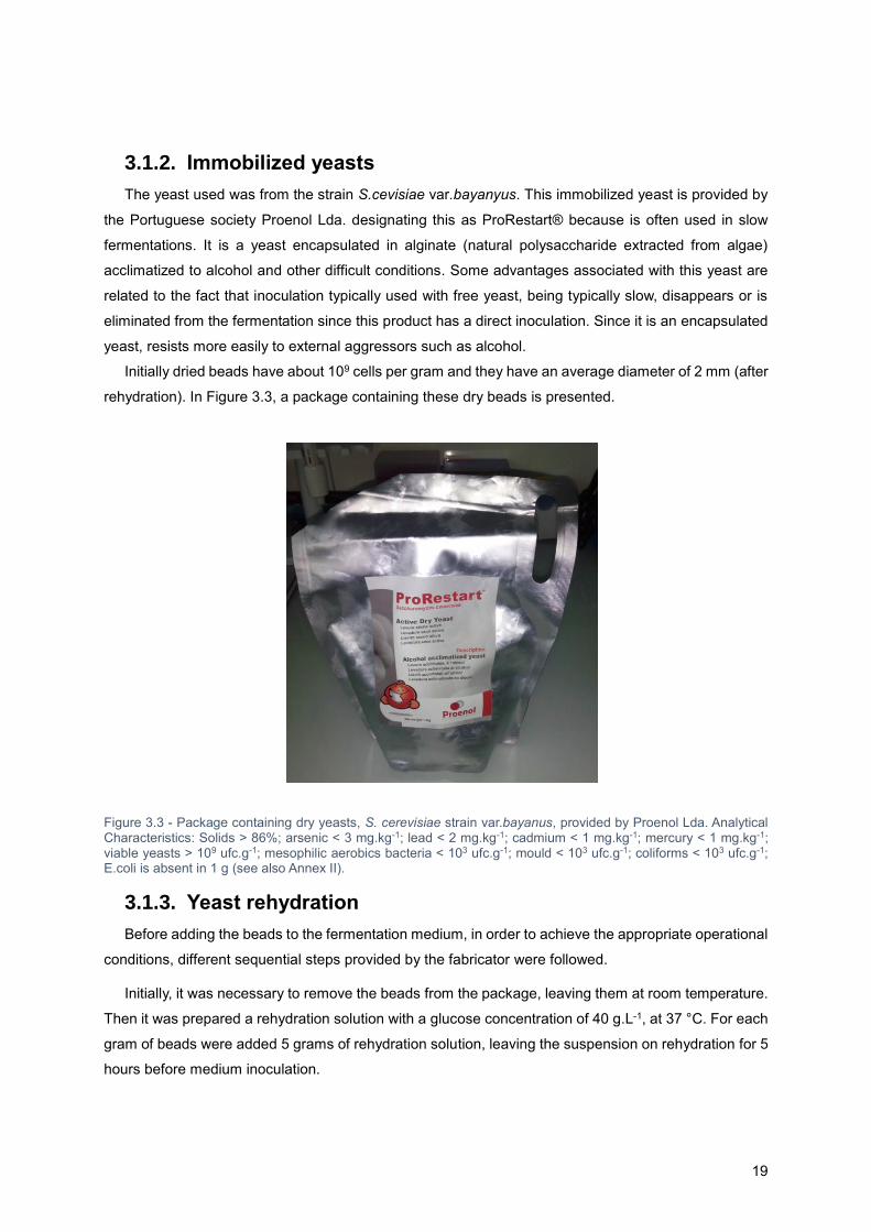
Initially dried beads have about 109 cells per gram and they have an average diameter of 2 mm (after
rehydration). In Figure 3.3, a package containing these dry beads is presented.
Figure 3.3 - Package containing dry yeasts, S. cerevisiae strain var.bayanus, provided by Proenol Lda. Analytical Characteristics: Solids > 86%; arsenic < 3 mg.kg-1; lead < 2 mg.kg-1; cadmium < 1 mg.kg-1; mercury < 1 mg.kg-1; viable yeasts > 109 ufc.g-1; mesophilic aerobics bacteria < 103 ufc.g-1; mould < 103 ufc.g-1; coliforms < 103 ufc.g-1; E.coli is absent in 1 g (see also Annex II).
3.1.3. Yeast rehydration
Before adding the beads to the fermentation medium, in order to achieve the appropriate operational
conditions, different sequential steps provided by the fabricator were followed.
Initially, it was necessary to remove the beads from the package, leaving them at room temperature.
Then it was prepared a rehydration solution with a glucose concentration of 40 g.L-1, at 37 °C. For each
gram of beads were added 5 grams of rehydration solution, leaving the suspension on rehydration for 5
hours before medium inoculation.
20
3.1.4. Batch fermentation
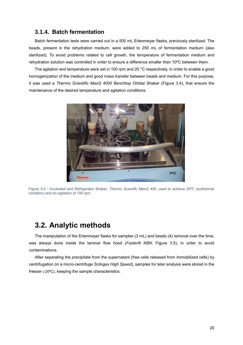
Batch fermentation tests were carried out in a 500 mL Erlenmeyer flasks, previously sterilized. The
beads, present in the rehydration medium, were added to 250 mL of fermentation medium (also
sterilized). To avoid problems related to cell growth, the temperature of fermentation medium and
rehydration solution was controlled in order to ensure a difference smaller than 10ºC between them.
The agitation and temperature were set in 100 rpm and 20 °C respectively, in order to enable a good
homogenization of the medium and good mass transfer between beads and medium. For this purpose,
it was used a Thermo Scientific MaxQ 4000 Benchtop Orbital Shaker (Figure 3.4), that ensure the
maintenance of the desired temperature and agitation conditions.
3.2. Analytic methods
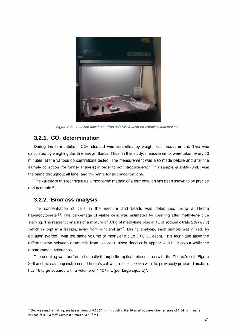
The manipulation of the Erlenmeyer flasks for samples (3 mL) and beads (4) removal over the time,
was always done inside the laminar flow hood (Faster® KBN, Figure 3.5), in order to avoid
contaminations.
After separating the precipitate from the supernatant (free cells released from immobilized cells) by
centrifugation (in a micro-centrifuge Scilogex High Speed), samples for later analysis were stored in the
freezer (-20ºC), keeping the sample characteristics.
Figure 3.4 - Incubated and Refrigerator Shaker, Thermo Scientifc MaxQ 400, used to achieve 20ºC (isothermal condition) and an agitation of 100 rpm.
* Because each small square has an area of 0.0025 mm2, counting the 16 small squares gives an area of 0.04 mm2 and a
volume of 0,004 mm3 (depth 0.1 mm) or 4.106 m.L-1. 21
3.2.1. CO2 determination
During the fermentation, CO2 released was controlled by weight loss measurement. This was
calculated by weighing the Erlenmeyer flasks. Thus, in this study, measurements were taken every 30
minutes, at the various concentrations tested. The measurement was also made before and after the
sample collection (for further analysis) in order to not introduce error. This sample quantity (3mL) was
the same throughout all time, and the same for all concentrations.
The validity of this technique as a monitoring method of a fermentation has been shown to be precise
and accurate 38.
3.2.2. Biomass analysis
The concentration of cells in the medium and beads was determined using a Thoma
haemocytometer39. The percentage of viable cells was estimated by counting after methylene blue
staining. The reagent consists of a mixture of 0.1 g of methylene blue in 1L of sodium citrate 2% (w / v)
,which is kept in a freezer, away from light and air40. During analysis, each sample was mixed, by
agitation (vortex), with the same volume of methylene blue (100 µL each). This technique allow the
differentiation between dead cells from live cells, since dead cells appear with blue colour while the
others remain colourless.
The counting was performed directly through the optical microscope (with the Thoma’s cell, Figure
3.6) and the counting instrument. Thoma’s cell which is filled in situ with the previously prepared mixture,
has 16 large squares with a volume of 4.10-6 mL (per large square)*.
Figure 3.5 – Laminar flow hood (Faster® KBN) used for sample's manipulation

22
The Thoma’s cell distribution is random, after application of the mixture. In this way each count had
its specificities. It was used a uniform method, always counting the same large square on the cell, usually
relying 3-5 large square in order to have a good representation. In order to validate the data, the number
of counted cells should be between 25 and 250 (live and dead). As the cell growth had been increasing
over time, it was necessary dilute the samples successively in order to respect the principle.
Since the final goal is to have comparable data, and knowing that depending on the counting, the
sample was further diluted or were counted more large squares, an equation was used in order to
calculate the cell concentration per mL of sample:
𝑋 ( 𝑐𝑒𝑙𝑙𝑠 𝑛𝑢𝑚𝑏𝑒𝑟 . 𝑚𝐿−1 ) = 𝐷𝑖𝑙𝑢𝑡𝑖𝑜𝑛 ×
𝑁𝑢𝑚𝑏𝑒𝑟 𝑜𝑓 𝐶𝑒𝑙𝑙𝑠 𝐶𝑜𝑢𝑛𝑡𝑒𝑑
𝑁𝑢𝑚𝑏𝑒𝑟 𝑜𝑓 𝐿𝑎𝑟𝑔𝑒 𝑆𝑞𝑢𝑎𝑟𝑒𝑠 𝐶𝑜𝑢𝑛𝑡𝑒𝑑×
1
4. 10−6
(19)
Throughout the experiments both immobilized cells (which grow within the beads) and free cells
(which are being released into the environment) were counted. To count the immobilized cells collected
in each time point (4 beads), it was necessary to dissolve the carrier material (alginate gel) in a solution
(1 mL) of sodium citrate 2 % (w / v), using an agitation by vortex (10 min.).
Figure 3.6 - Instruments for Biomass Analysis: 1- The Optical microscope Leitz®, model Laborlux 12; 2- Counting instrument: red button and white button pressed for every dead and living cell respectively.
1
2
Figure 3.7 - Thoma's cell filled with solution (50%(v/v) sample + 50%(v/v)methylene blue) used in the measures throughout experiments

23
3.2.3. HPLC
The HPLC was used to measure sugars (total) and ethanol presents in the sample. HPLC
measurements were performed on columns Rezex ROA-H+, 250 mm long x 4.6 mm wide, with a mobile
phase of H2SO4 1.87 mmol.L-1 circulating 170 µL.min-1 at 30ºC, in a Thermo Scientific Acella™ HPLC
system (Thermo Fischer Corporation) mounted with an external detection device (Figure 3.8).
Before starting the measurements related to ethanol and sugars (glucose, sucrose and fructose),
standard solutions were prepared. It was weighed 500 mg (of each standard compound: ethanol,
sucrose, fructose and glucose) in Sartorius CP214 Analytical Balance (more precision) and then were
added 50 mL of water, performing a concentration of 10 g.L-1 (for each compound). Successive dilutions
were done to prepare solutions of 8,6,4,2 g.L-1 (concentration of each standard compound). To minimize
errors in the detection device, water samples were also prepared.
References ranges and its graphics, important in data processing are presented in Annex III (it
should be noted that the samples were diluted 1:20, in order to have values within our reference range).
The autosampler vials, where the samples and reference solutions are introduced, are shown in Figure
3.9.
Figure 3.8 - HPLC system
Figure 3.9 - Autosampler vials for HPLC, filled with the samples and standard solutions

24
3.2.4. DNS method
This method was used to dose and monitor the consumption of reducing sugars. Thus, this method
was as proof of the data collected from HPLC. The method principle says that the reducing sugars react
with DNS (dinitrosalicylic acid reagent: dinitrosalicylic acid; rochelle salt; phenol; sodium bisulphite and
sodium hydroxide) by reducing it to 3-amino-5-nitrosalicylic acid 41. This reaction is accompanied by a
colour change, from a yellow colour (corresponding to the DNS reagent, Figure 3.10) into an orange /
red colour.
Before determination of the reducing sugars in the samples, a calibration curve was prepared. For
this purpose, the protocol followed consists on:
Turning the thermostat bath at 80 ° C;
Preparation of a glucose mother solution (Sm) , 50 g.L-1 (high concentration in order to
increase the sensitivity of the method). Weight 10 grams of glucose and transferred to a
volumetric flask with 200 ml of distilled water;
Preparation of 1 ml reference solution for 40; 30; 20; 10; 5; 1; 0.5 and 0 g.L-1 of glucose.(
S1,…, S8, respectively).For example:
o For the 40 g.L-1 solution (S1): In an Eppendorf tube, placing 800 µL of Sm and 200μl
of water;
o For the 0 g.L-1 solution (S8): : 1 mL of distilled water.
Sugars Reaction:
o Preparation of 9 Eppendorf tubes for each solution (Sm; S1, S2, S3, S4, S5,S6,S7,S8);
o Placing in each tube, 950μl of DNS using the “special” pipette;
o Placing 50 µL of each solution in corresponding Eppendorf tubes:
o Placing tubes in 3 minutes thermostat bath at 80 ° C.
Reading the absorbance of each of the reference solutions in the spectrophotometer
Jenway 7315.
Figure 3.10 - DNS Reagent used for measurement of reducing sugars.

25
The obtained calibration curve obtained is reported in (Figure 3.11).
Figure 3.11 - Calibration curve for glucose and the corresponding equation.
Using the linear regression obtained by plotting the absorbance vs concentration for the references
solutions, it was possible to determine the concentrations of reducing sugars (glucose and fructose) in
the fermentation samples. In the case of samples that showed higher absorbance values compared to
the range measured for the standard solution, serial dilutions were made in order to obtain reasonable
values (absorbance less than 2).
For samples preparation (reaction with DNS reagent) was performed the same protocol used for the
standard solutions. Figure 3.12 shows the equipment used for the preparation of this reaction.
Figure 3.12 - Material used for preparing the reaction of the samples with DNS reagent : 1-Eppendorfs filled with 950 µL DNS reagent; 2- Fermentation samples; 3- “Special” pipette; 4- Beaker with DNS reagent ( yellow )
1
2
3 4
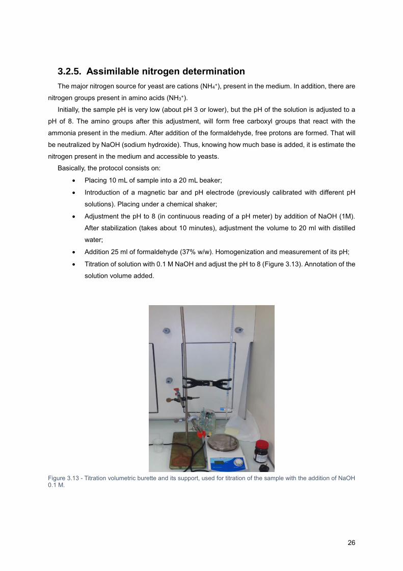
26
3.2.5. Assimilable nitrogen determination
The major nitrogen source for yeast are cations (NH4+), present in the medium. In addition, there are
nitrogen groups present in amino acids (NH3+).
Initially, the sample pH is very low (about pH 3 or lower), but the pH of the solution is adjusted to a
pH of 8. The amino groups after this adjustment, will form free carboxyl groups that react with the
ammonia present in the medium. After addition of the formaldehyde, free protons are formed. That will
be neutralized by NaOH (sodium hydroxide). Thus, knowing how much base is added, it is estimate the
nitrogen present in the medium and accessible to yeasts.
Basically, the protocol consists on:
Placing 10 mL of sample into a 20 mL beaker;
Introduction of a magnetic bar and pH electrode (previously calibrated with different pH
solutions). Placing under a chemical shaker;
Adjustment the pH to 8 (in continuous reading of a pH meter) by addition of NaOH (1M).
After stabilization (takes about 10 minutes), adjustment the volume to 20 ml with distilled
water;
Addition 25 ml of formaldehyde (37% w/w). Homogenization and measurement of its pH;
Titration of solution with 0.1 M NaOH and adjust the pH to 8 (Figure 3.13). Annotation of the
solution volume added.
Figure 3.13 - Titration volumetric burette and its support, used for titration of the sample with the addition of NaOH 0.1 M.
27
3.3. Computational work
The computational methods used in this work are very important in order to use and interpret the
experiment data. Since it works with kinetic models, integration and parameter estimation are the engine
of this work. This was made using Matlab® software42 and the Microsoft Excel® program.
The Excel numerical integration was performed essentially using the Euler method:
𝑦𝑛+1 = 𝑦𝑛 + ℎ𝑓(𝑡𝑛, 𝑦𝑛) (20),
where 𝑓(𝑡𝑛, 𝑦𝑛) = 𝑦′(𝑡) and 𝑡𝑛 = 𝑡0 + 𝑛ℎ .
To identify the value of a parameter, the most commonly used formula is the method of least squares,
represented by the following formula 43 :
where J is the objective function; δexp represents the measurements collected from the experiments;
δmod represents the prediction result by the model corresponding to the point of measurement in
experimentation; θ is the parameter to be determined; N is the number of measurements. The Solver
function of Excel is used to minimize the Equation (21).
Once the Excel program presents some limitations (in terms of iterations), it had been written and
developed a program in Matlab. In this computing environment, simulations and parameter estimates
were made, relating the experience studied with the kinetic model.
It was used a program developed in modelling applied to the dynamics of microbial populations,
developed at LGC (Laboratoire de Genie Chimique) where this work was done. This aid program,
termed as Modelight44 is a workspace that contains four types of files:
Data: corresponding to the file where the experimental results are placed. In this study were:
the substrate (S); the product, ethanol (P); Biomass (X) and nitrogen (N).
Functions: that corresponds to the repertoire of auxiliary functions corresponding to the
variables involved in the process;
Models: which corresponds to the description of ordinary differential equations, which are
based on the descriptive of the kinetic model. It is this file that also process variables and
parameters are defined;
Results: That corresponds to the file where the results of the simulations are grouped. This
output file correspond to the values of variables, functions and settings that have been
determined by calculation.
Modelight allows testing of dynamic models quickly, from the only knowledge of their variables, their
parameters and differential equations of the system that defines them. No algorithmic programming is
required. This software has two main features:
(𝜃) = 𝑚𝑖𝑛 ∑(𝛿𝑒𝑥𝑝
𝑁
𝑡=1
(𝑡) − 𝛿𝑚𝑜𝑑(𝑡, 𝜃))2 (21)
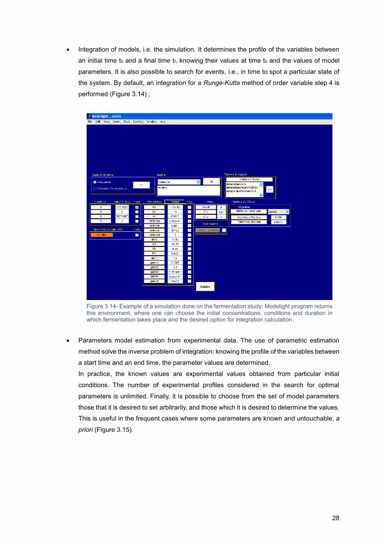
28
Integration of models, i.e. the simulation. It determines the profile of the variables between
an initial time t0 and a final time tf, knowing their values at time t0 and the values of model
parameters. It is also possible to search for events, i.e., in time to spot a particular state of
the system. By default, an integration for a Runge-Kutta method of order variable step 4 is
performed (Figure 3.14) ;
Parameters model estimation from experimental data. The use of parametric estimation
method solve the inverse problem of integration: knowing the profile of the variables between
a start time and an end time, the parameter values are determined.
In practice, the known values are experimental values obtained from particular initial
conditions. The number of experimental profiles considered in the search for optimal
parameters is unlimited. Finally, it is possible to choose from the set of model parameters
those that it is desired to set arbitrarily, and those which it is desired to determine the values.
This is useful in the frequent cases where some parameters are known and untouchable, a
priori (Figure 3.15).
Figure 3.14- Example of a simulation done on the fermentation study: Modelight program returns this environment, where one can choose the initial concentrations, conditions and duration in which fermentation takes place and the desired option for integration calculation.

29
Figure 3.15 - Example of a parametric estimation done on the fermentation study: Modelight program returns this environment, where one can choose the initial concentrations, conditions and duration in which fermentation takes place and the desired option for integration calculation. The window returned by the program also lets you select which parameters one wishes to fix / change and the ranges where these can be calculated.
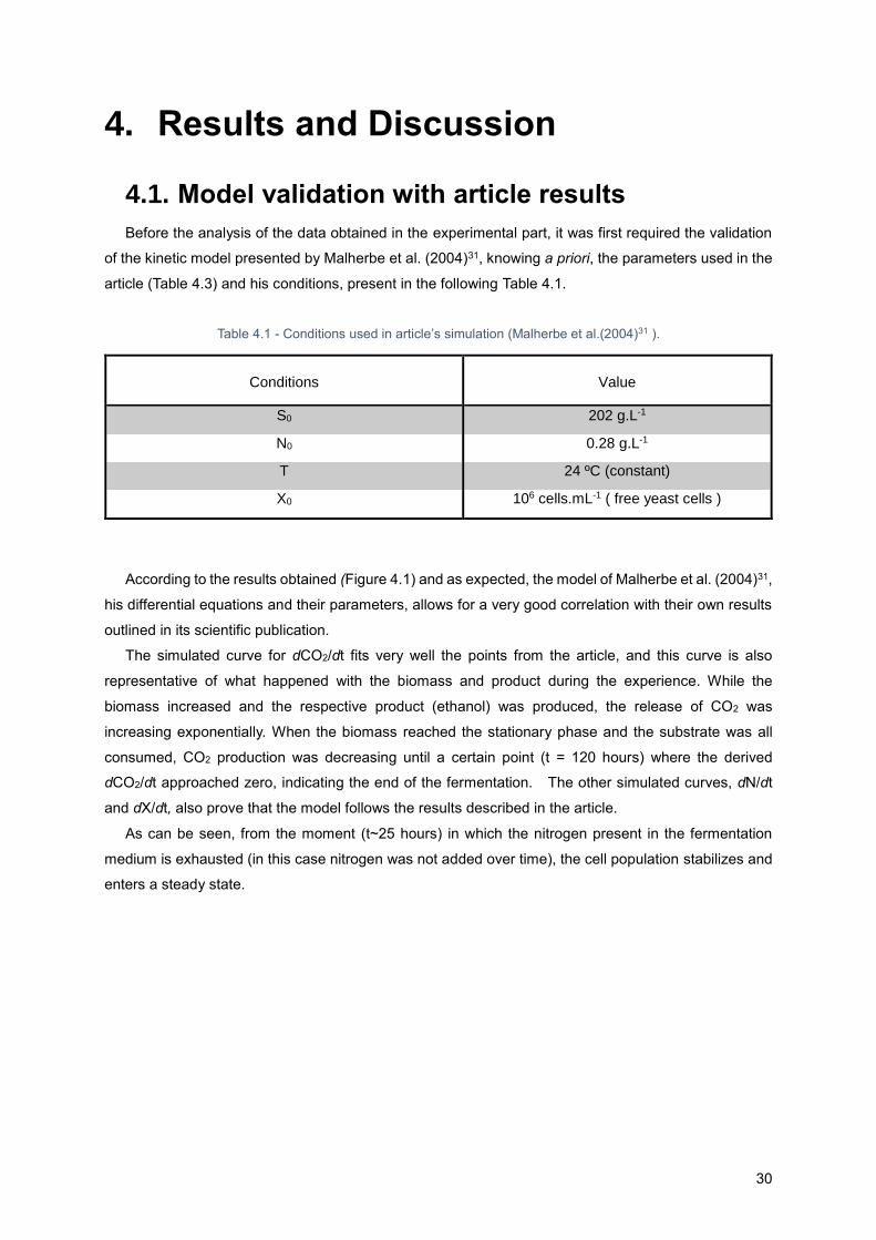
30
4. Results and Discussion
4.1. Model validation with article results
Before the analysis of the data obtained in the experimental part, it was first required the validation
of the kinetic model presented by Malherbe et al. (2004)31, knowing a priori, the parameters used in the
article (Table 4.3) and his conditions, present in the following Table 4.1.
Table 4.1 - Conditions used in article’s simulation (Malherbe et al.(2004)31 ).
According to the results obtained (Figure 4.1) and as expected, the model of Malherbe et al. (2004)31,
his differential equations and their parameters, allows for a very good correlation with their own results
outlined in its scientific publication.
The simulated curve for dCO2/dt fits very well the points from the article, and this curve is also
representative of what happened with the biomass and product during the experience. While the
biomass increased and the respective product (ethanol) was produced, the release of CO2 was
increasing exponentially. When the biomass reached the stationary phase and the substrate was all
consumed, CO2 production was decreasing until a certain point (t = 120 hours) where the derived
dCO2/dt approached zero, indicating the end of the fermentation. The other simulated curves, dN/dt
and dX/dt, also prove that the model follows the results described in the article.
As can be seen, from the moment (t~25 hours) in which the nitrogen present in the fermentation
medium is exhausted (in this case nitrogen was not added over time), the cell population stabilizes and
enters a steady state.
Conditions
Value
S0 202 g.L-1
N0 0.28 g.L-1
T 24 ºC (constant)
X0 106 cells.mL-1 ( free yeast cells )
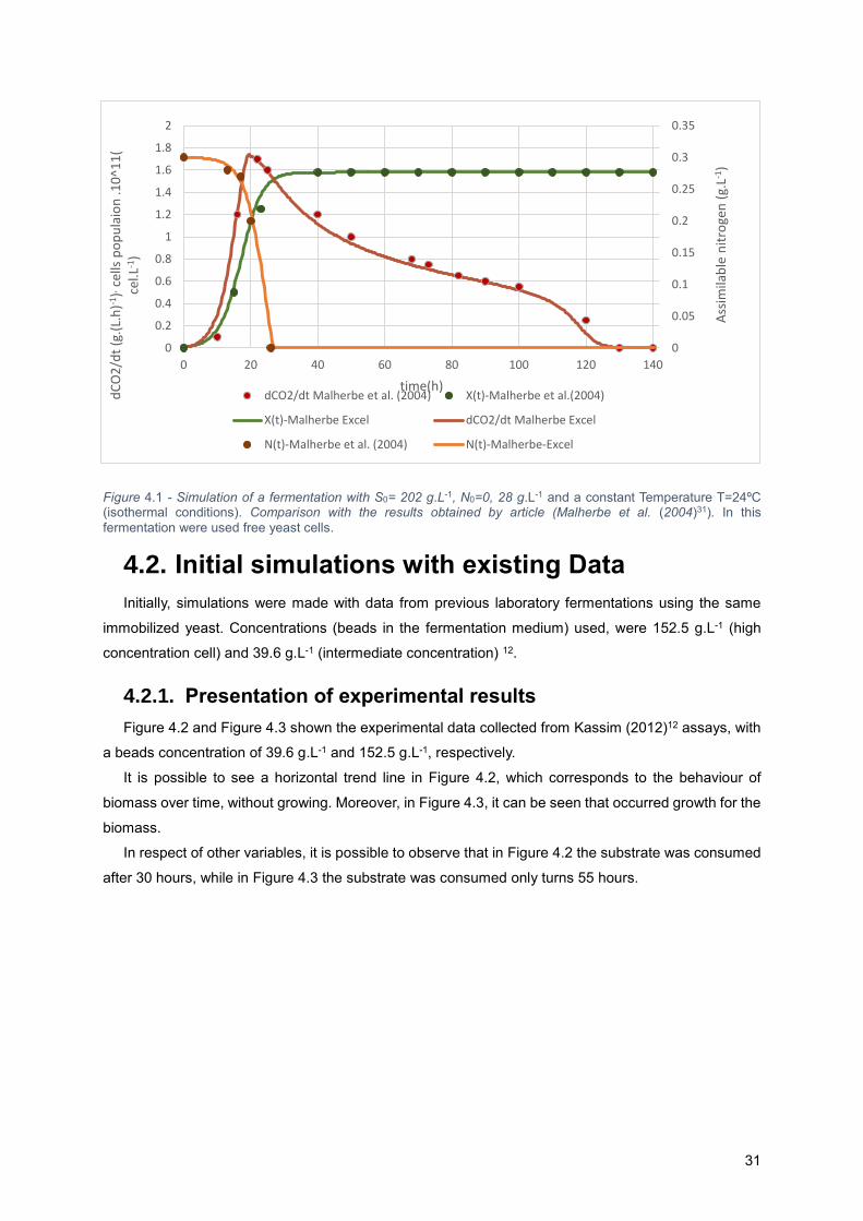
31
Figure 4.1 - Simulation of a fermentation with S0= 202 g.L-1, N0=0, 28 g.L-1 and a constant Temperature T=24ºC (isothermal conditions). Comparison with the results obtained by article (Malherbe et al. (2004)31). In this
fermentation were used free yeast cells.
4.2. Initial simulations with existing Data
Initially, simulations were made with data from previous laboratory fermentations using the same
immobilized yeast. Concentrations (beads in the fermentation medium) used, were 152.5 g.L-1 (high
concentration cell) and 39.6 g.L-1 (intermediate concentration) 12.
4.2.1. Presentation of experimental results
Figure 4.2 and Figure 4.3 shown the experimental data collected from Kassim (2012)12 assays, with
a beads concentration of 39.6 g.L-1 and 152.5 g.L-1, respectively.
It is possible to see a horizontal trend line in Figure 4.2, which corresponds to the behaviour of
biomass over time, without growing. Moreover, in Figure 4.3, it can be seen that occurred growth for the
biomass.
In respect of other variables, it is possible to observe that in Figure 4.2 the substrate was consumed
after 30 hours, while in Figure 4.3 the substrate was consumed only turns 55 hours.
0
0.05
0.1
0.15
0.2
0.25
0.3
0.35
0
0.2
0.4
0.6
0.8
1
1.2
1.4
1.6
1.8
2
0 20 40 60 80 100 120 140
Ass
imila
ble
nit
roge
n (
g.L-1
)
dC
O2
/dt
(g.(
L.h
)-1),
cells
po
pu
laio
n .1
0^1
1(
cel.L
-1)
time(h)dCO2/dt Malherbe et al. (2004) X(t)-Malherbe et al.(2004)
X(t)-Malherbe Excel dCO2/dt Malherbe Excel
N(t)-Malherbe et al. (2004) N(t)-Malherbe-Excel
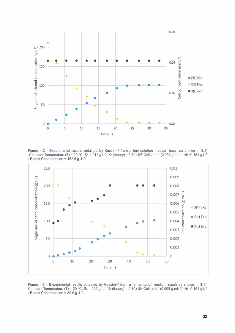
32
Figure 4.2 - Experimental results obtained by Kassim12 from a fermentation medium (such as shown in 3.1) .Constant Temperature (T) = 20 °C; S0 = 212 g.L-1; X0 (theory) = 3.81x10⁸ Cells.mL-1 (0.035 g.mL-1); N0=0.161 g.L-1 ; Beads Concentration = 152.5 g .L-1.
Figure 4.3 - Experimental results obtained by Kassim12 from a fermentation medium (such as shown in 3.1). Constant Temperature (T) = 20 °C; S0 = 205 g.L-1; X0 (theory) = 9.89x10⁷ Cells.mL-1 (0.008 g.mL-1); N0=0.161 g.L-1 ; Beads Concentration = 39.6 g .L-1.
0.01
0.02
0.03
0.04
0
50
100
150
200
0 5 10 15 20 25 30 35
Cel
l co
nce
ntr
atio
n (
g.m
L-1)
Suga
r an
d e
than
ol c
on
cen
trat
ion
(g.
L-1)
time(h)
P(t) Exp.
S(t) Exp.
X(t) exp.
0
0.001
0.002
0.003
0.004
0.005
0.006
0.007
0.008
0.009
0.01
0
50
100
150
200
250
0 10 20 30 40 50 60
Cel
l co
nce
ntr
atio
n (
g.m
L-1)
Suga
r an
d e
than
ol c
on
cen
trat
ion
(g.
L-1
)
time(h)
S(t) Exp.
P(t) Exp.
X(t) Exp.
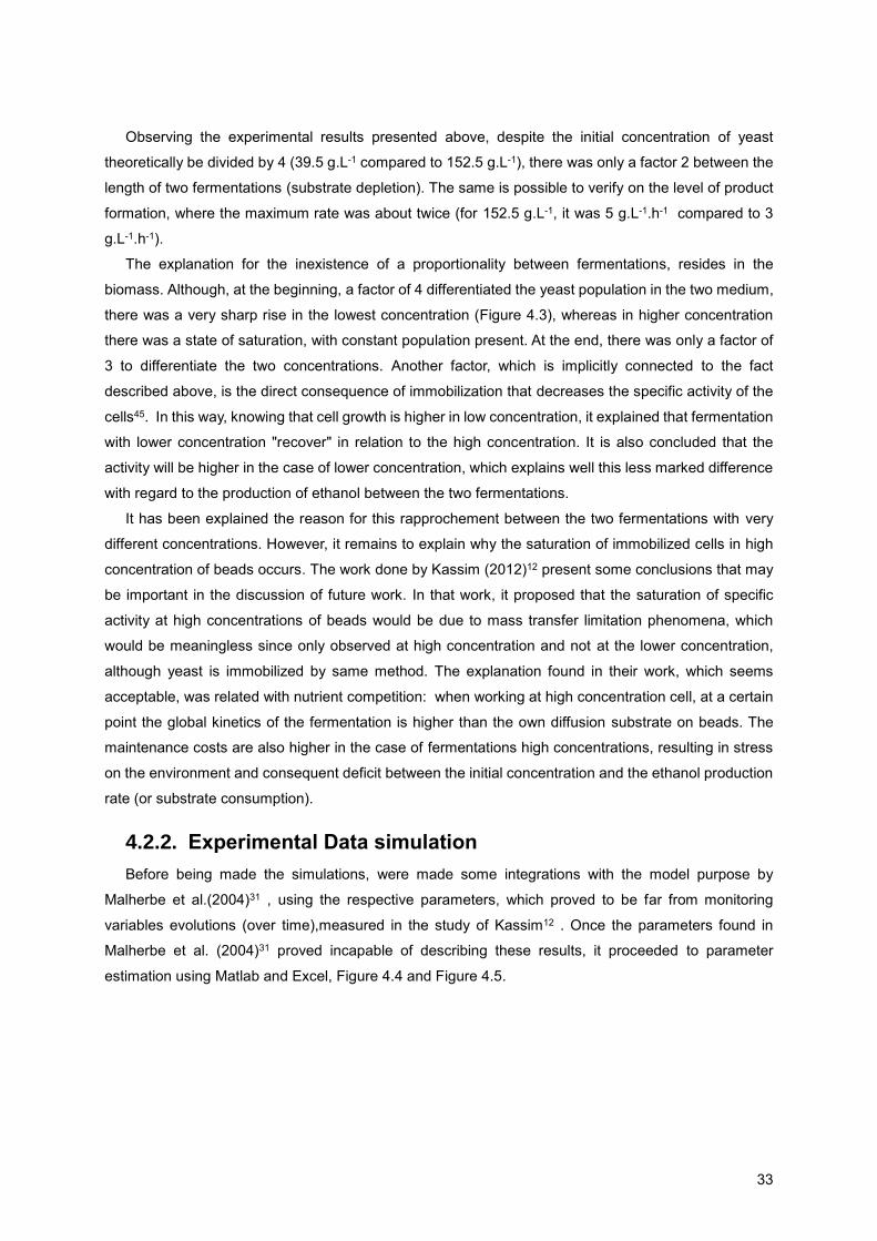
33
Observing the experimental results presented above, despite the initial concentration of yeast
theoretically be divided by 4 (39.5 g.L-1 compared to 152.5 g.L-1), there was only a factor 2 between the
length of two fermentations (substrate depletion). The same is possible to verify on the level of product
formation, where the maximum rate was about twice (for 152.5 g.L-1, it was 5 g.L-1.h-1 compared to 3
g.L-1.h-1).
The explanation for the inexistence of a proportionality between fermentations, resides in the
biomass. Although, at the beginning, a factor of 4 differentiated the yeast population in the two medium,
there was a very sharp rise in the lowest concentration (Figure 4.3), whereas in higher concentration
there was a state of saturation, with constant population present. At the end, there was only a factor of
3 to differentiate the two concentrations. Another factor, which is implicitly connected to the fact
described above, is the direct consequence of immobilization that decreases the specific activity of the
cells45. In this way, knowing that cell growth is higher in low concentration, it explained that fermentation
with lower concentration "recover" in relation to the high concentration. It is also concluded that the
activity will be higher in the case of lower concentration, which explains well this less marked difference
with regard to the production of ethanol between the two fermentations.
It has been explained the reason for this rapprochement between the two fermentations with very
different concentrations. However, it remains to explain why the saturation of immobilized cells in high
concentration of beads occurs. The work done by Kassim (2012)12 present some conclusions that may
be important in the discussion of future work. In that work, it proposed that the saturation of specific
activity at high concentrations of beads would be due to mass transfer limitation phenomena, which
would be meaningless since only observed at high concentration and not at the lower concentration,
although yeast is immobilized by same method. The explanation found in their work, which seems
acceptable, was related with nutrient competition: when working at high concentration cell, at a certain
point the global kinetics of the fermentation is higher than the own diffusion substrate on beads. The
maintenance costs are also higher in the case of fermentations high concentrations, resulting in stress
on the environment and consequent deficit between the initial concentration and the ethanol production
rate (or substrate consumption).
4.2.2. Experimental Data simulation
Before being made the simulations, were made some integrations with the model purpose by
Malherbe et al.(2004)31 , using the respective parameters, which proved to be far from monitoring
variables evolutions (over time),measured in the study of Kassim12 . Once the parameters found in
Malherbe et al. (2004)31 proved incapable of describing these results, it proceeded to parameter
estimation using Matlab and Excel, Figure 4.4 and Figure 4.5.
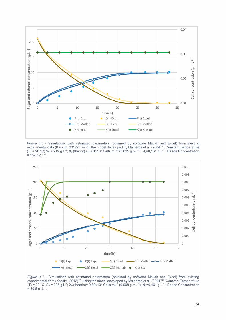
34
Figure 4.4 - Simulations with estimated parameters (obtained by software Matlab and Excel) from existing
experimental data (Kassim, 2012)12, using the model developed by Malherbe et al. (2004)31. Constant Temperature (T) = 20 °C; S0 = 205 g.L-1; X0 (theoric)= 9.89x10⁷ Cells.mL-1 (0.008 g.mL-1); N0=0,161 g.L-1 ; Beads Concentration = 39.6 g .L-1.
Figure 4.5 - Simulations with estimated parameters (obtained by software Matlab and Excel) from existing experimental data (Kassim, 2012)12, using the model developed by Malherbe et al. (2004)31. Constant Temperature (T) = 20 °C; S0 = 212 g.L-1; X0 (theory) = 3.81x10⁸ Cells.mL-1 (0.035 g.mL-1); N0=0,161 g.L-1 ; Beads Concentration = 152.5 g.L-1.
0.01
0.02
0.03
0.04
0
50
100
150
200
0 5 10 15 20 25 30 35
Cel
l co
nce
ntr
atio
n (
g.m
L-1)
Suga
r an
d e
than
ol c
on
cen
trat
ion
(g.
L-1)
time(h)
P(t) Exp. S(t) Exp. P(t) Excel
P(t) Matlab S(t) Excel S(t) Matlab
X(t) exp. X(t) Excel X(t) Matlab
0
0.001
0.002
0.003
0.004
0.005
0.006
0.007
0.008
0.009
0.01
0
50
100
150
200
250
0 10 20 30 40 50 60Suga
r an
d e
than
ol c
on
cen
trat
ion
(g.
L-1)
time(h)
S(t) Exp. P(t) Exp. S(t) Excel S(t) Matlab P(t) Matlab
P(t) Excel X(t) Excel X(t) Matlab X(t) Exp.
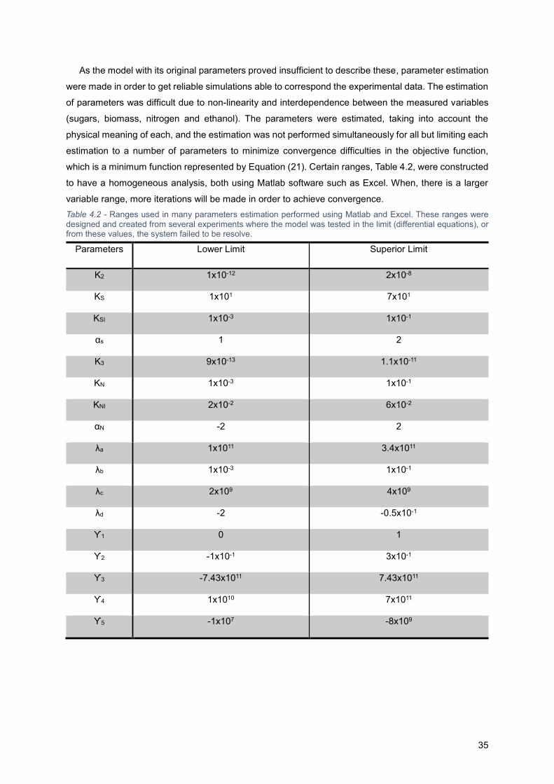
35
As the model with its original parameters proved insufficient to describe these, parameter estimation
were made in order to get reliable simulations able to correspond the experimental data. The estimation
of parameters was difficult due to non-linearity and interdependence between the measured variables
(sugars, biomass, nitrogen and ethanol). The parameters were estimated, taking into account the
physical meaning of each, and the estimation was not performed simultaneously for all but limiting each
estimation to a number of parameters to minimize convergence difficulties in the objective function,
which is a minimum function represented by Equation (21). Certain ranges, Table 4.2, were constructed
to have a homogeneous analysis, both using Matlab software such as Excel. When, there is a larger
variable range, more iterations will be made in order to achieve convergence.
Table 4.2 - Ranges used in many parameters estimation performed using Matlab and Excel. These ranges were
designed and created from several experiments where the model was tested in the limit (differential equations), or from these values, the system failed to be resolve.
Parameters Lower Limit Superior Limit
K2 1x10-12 2x10⁻⁸
KS 1x101 7x101
KSI 1x10⁻³ 1x10⁻¹
αs 1 2
K3 9x10-13 1.1x10⁻¹¹
KN 1x10⁻³ 1x10⁻¹
KNI 2x10⁻² 6x10⁻²
αN -2 2
λa 1x10¹¹ 3.4x10¹¹
λb 1x10⁻³ 1x10⁻¹
λc 2x10⁹ 4x10⁹
λd -2 -0.5x10⁻¹
ϒ1 0 1
ϒ2 -1x10⁻¹ 3x10⁻¹
ϒ3 -7.43x10¹¹ 7.43x10¹¹
ϒ4 1x10¹⁰ 7x10¹¹
ϒ5 -1x10⁷ -8x10⁹

*It is known that the purpose of the model was to be applied to other conditions (after determining the parameters) .However, there was no universality and it was made parametric estimation, since it cannot validate the model with the data provided by Kassim (2012)12. 36
The strategy used for both software was to start by “blocking” all the parameters involved in the
differential equations of the model, except those related to the growth of the biomass, ie dX/dt ((11). The
functions, linked to cell growth, are K1 (T) and Xmax (Ninit), which relate to a linear function and a
polynomial function, respectively. The first function involved the parameters ϒ1 and ϒ2 (K1 (t) = ϒ1T-
ϒ2), while the second, as demonstrated in Equation (13), involved the parameters ϒ3, ϒ4 and ϒ5. These
parameters (as will be discussed subsequently) were determined in Malherbe et al. (2004)31 by
parameter estimation also using a similar methodology to the proposal (simultaneous estimation of a
limited number of parameters).However, it was performed at 24 °C (T) with a certain initial concentration
of biomass (free yeast),X0, and from a certain initial concentration of assimilable nitrogen ( Ninit)*.
Estimations were made solely directed to the parameters of the above functions (K1 (T) and Xmax
(Ninit)), in order to correct the correlation between biomass measured experimentally and the calculated
by the model. The data related to the estimation are represented in Table 4.3. Referring to Figure 4.4
(higher concentration) is perceptible to note that the parameters calculated by the two tools are similar
(in most cases equal), since the curves are similar and overlapping. The parameters change from the
original model was evident, because the model assumes a cell growth (as it was designed to lower cell
concentrations) that did not happen in the case of the estimation using a concentration of 152.6 g.L-1 of
beads. Once corrected biomass, X (t), there were changes also in other system equations, since this
biomass are interdependent. Changes in other parameters (not all) were also performed.
Observing the behaviour of the substrate (S(t)), where they enter 𝑁𝑆𝑇 and 𝑉𝑆𝑇 functions (Equation(9)),
it can see a better fit in relation to the simulation made with parameters estimated by Matlab (Figure 4.5
and Figure 4.4). Function 𝑁𝑆𝑇 is represented by the Equations (15)(16),discriminating the number of
hexose transporters. It is important to note that is considered λ0 equal to one unit in the Equation (16),
since nitrogen is not added during fermentation in Kassim (2012)12 experiments. Thus the λ parameters
were estimated, as shown in Table 4.3. Simultaneously, it estimated the parameters for 𝑉𝑆𝑇 function
(Equation (14)), which is a nonlinear regression model related do the hexose transport, where were
estimated the parameters: K2; KS; KSI and αs . For some of these parameters can be seen that these are
physically measurable parameters, KS is a constant affinity for sugar transporters (expressed in g.L-1)
and KSI is the constant for inhibition for the sugar transporters in the presence of ethanol (expressed in
L.g-1), which led to the research and care in the preparation of the ranges of these parameters in your
estimation (Table 4.2).
At the same time that it made the estimation of parameters involved in the differential equation
relating to substrate consumption S(t), it was also made the estimation of 𝜈𝑁 function parameters, which
describes the active transport of nitrogen (Equation (17)), belonging to the differential equation relating
to nitrogen assimilable existing in the medium (Equation (10)).The function 𝜈𝑁 is written in the same way
as the function 𝑉𝑆𝑇, however the parameters are related to nitrogen ( it was made the same preparation
of the ranges).

37
The reason for done this estimation, simultaneously for S(t) and N(t) parameters,was related to the
fact that the value of N(t) enters into the fucntion 𝑁𝑆𝑇 (respect to the substrate), and thus a simulation
made a posteriori to the nitrogen (N(t)) would have a direct impact on the equation of the substrate,
affecting its fit. In turn, the biomass was initially set, as already mentioned it was determined a priori.
It is assumed that once was adjusted the substrate consumption between the model and
experimental data, the product (P(t)) calculated by simulation for each of the software will also adjusted
on the same extent.There was,again, a better fit for the product estimated by Matlab.
An overview to the Table 4.3, it can be seen that most parametric changes were in the parameters
relating to cell growth (ϒ), which is explained by the use of higher concentrations than those related to
article Malherbe et al. (2004)31, which used free cells inoculate 106 cells.mL-1 (2 and 3 times smaller
than the cells inoculated beads in concentrations of 39.6 g.L-1 and 152.6 g.L-1, respectively).
Table 4.3 - Calculated parameters in order to adjust the model to the experimental data. The original parameters are presented (from the article Malherbe et al. (2004)31) and the calculated parameters depending on the used programs for two bead concentrations.
Parameters
Originally calculated (Article)
Estimation by Excel Beads
Concentration 152.6 g.L-1
Estimation by Matlab Beads Concentration
152.6 g.L-1
Estimation by Excel Beads Concentration
39.6 g.L-1
Estimation by Matlab Beads Concentration
39.6 g.L-1
k2 1.05x10⁻¹¹ 9.58x10⁻⁹ 9.58x10⁻⁹ 3.05x10⁻¹¹ 3.05x10⁻¹¹
Ks 1.50x101 5.93x101 5.93x101 3.11x101 1.50x101
Ksi 1.20x10⁻² 2.26x10⁻² 2.20x10⁻² 9.42x10⁻³ 1.20x10⁻²
αs 1.25 1.26 1.26 1.25 1.25
k3 1.00x10⁻¹² 5.84x10⁻¹³ 5.83x10⁻¹³ 1.00x10⁻¹² 1.00x10⁻¹²
KN 3.00x10⁻² 3.22x10⁻² 3.21x10⁻² 3.52x10⁻⁵ 3.50x10⁻⁵
KNI 3.50x10⁻² 3.46x10⁻² 3.40x10⁻² 3.50x10⁻² 3.11x10⁻²
αn 1.50 6.53x10⁻¹ 6.50x10⁻¹ -1.04 1.50
λa 3.35x10¹¹ 1.93x10¹¹ 1.93x10¹¹ 3.35x10¹¹ 3.35x10¹¹
λb 6.10x10⁻² 1.11x10⁻¹ 1.11x10⁻¹ 3.56x101 3.58x101
λc 3.00x10⁹ 2.80x10+9 2.80x10⁹ 3.00x10⁹ 3.00x10⁹
λd -1.00 -3.25x10⁻¹ -3.20x10⁻¹ 4.79x10⁻¹ 4.90x10⁻¹
ϒ1 2.87x10⁻² 2.18x10⁻² 2.10x10⁻² 1.81x10⁻² 1.60x10⁻¹
ϒ2 -3.76x10⁻¹ -4.36x10⁻¹ -4.36x10⁻¹ 4.52x10⁻² 5.10x10⁻²
ϒ3 -6.49x10¹¹ -7.43 -7.43 -7.43 -7.43
ϒ4 6.98x10¹¹ 1.69x10¹⁰ 1.69x10¹⁰ 1.00 1.00
ϒ5 7.00x10+9 -1.04x10⁹ -1.04x10⁹ 4.41x10⁸ 4.41x10⁸
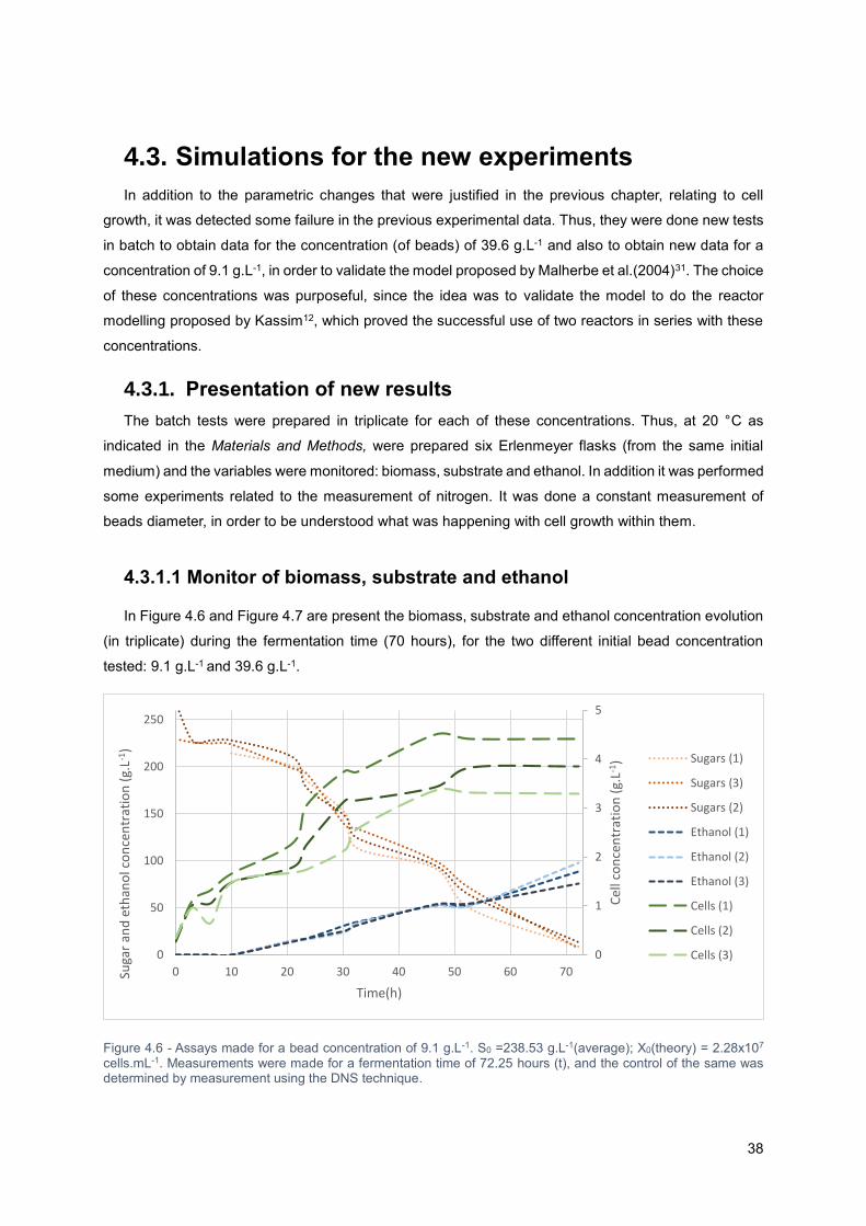
38
4.3. Simulations for the new experiments
In addition to the parametric changes that were justified in the previous chapter, relating to cell
growth, it was detected some failure in the previous experimental data. Thus, they were done new tests
in batch to obtain data for the concentration (of beads) of 39.6 g.L-1 and also to obtain new data for a
concentration of 9.1 g.L-1, in order to validate the model proposed by Malherbe et al.(2004)31. The choice
of these concentrations was purposeful, since the idea was to validate the model to do the reactor
modelling proposed by Kassim12, which proved the successful use of two reactors in series with these
concentrations.
4.3.1. Presentation of new results
The batch tests were prepared in triplicate for each of these concentrations. Thus, at 20 °C as
indicated in the Materials and Methods, were prepared six Erlenmeyer flasks (from the same initial
medium) and the variables were monitored: biomass, substrate and ethanol. In addition it was performed
some experiments related to the measurement of nitrogen. It was done a constant measurement of
beads diameter, in order to be understood what was happening with cell growth within them.
4.3.1.1 Monitor of biomass, substrate and ethanol
In Figure 4.6 and Figure 4.7 are present the biomass, substrate and ethanol concentration evolution
(in triplicate) during the fermentation time (70 hours), for the two different initial bead concentration
tested: 9.1 g.L-1 and 39.6 g.L-1.
Figure 4.6 - Assays made for a bead concentration of 9.1 g.L-1. S0 =238.53 g.L-1(average); X0(theory) = 2.28x10⁷ cells.mL-1. Measurements were made for a fermentation time of 72.25 hours (t), and the control of the same was determined by measurement using the DNS technique.
0
1
2
3
4
5
0
50
100
150
200
250
0 10 20 30 40 50 60 70
Cel
l co
nce
ntr
atio
n (
g.L-1
)
Suga
r an
d e
than
ol c
on
cen
trat
ion
(g.
L-1)
Time(h)
Sugars (1)
Sugars (3)
Sugars (2)
Ethanol (1)
Ethanol (2)
Ethanol (3)
Cells (1)
Cells (2)
Cells (3)

39
Figure 4.7 - Assays made for a bead concentration of 39.6 g.L-1. S0 =223.54 g.L-1(average); X0(theory) = 9.89x10⁷
cells.mL-1. Measurements were made for a fermentation time of 72.25 hours (t), and the control of the same was determined by measurement using the DNS technique.
In Figure 4.6 can be seen a great increase in biomass. It was accompanied by the increasing of the
substrate consumption rate and consequently, the formation of the product, which reaches a value of
100 g.L-1 of ethanol. In Figure 4.7, it can see a sharp growth of the biomass at the start of fermentation,
but from 20 hours it began to stabilize. After 50 hours of fermentation, there was a marked decrease in
substrate consumption and product formation thereby. It is also important to note that the data obtained
in this experiment for the concentration of 39.6 g.L-1, Figure 4.7, showed some differences with previous
data from Kassim12.
Comparing Figure 4.6 and Figure 4.7, it can be seen, that, observing the curve related with the
evolution of substrate (S), the fermentation correspondent to an initial lower concentration (9.1 g.L-1) ,
Figure 4.6, occurred in a slower way than the fermentation related to the concentration previously
studied (39.6 g.L-1), Figure 4.7, as the substrate is depleted faster ( at 70 hours, there was not substrate
for the higher concentration, while the other remained a substrate) due to the fact that there was also
more biomass initially present in the medium, and the ethanol yield is slightly higher, too. However, and
since the production of ethanol is increased, the inhibitory effect also feels earlier in relation to the lower
concentration, as can be seen comparing the slope (rate) of curves relating to substrate consumption
from 35 hours in both Figures.
Analyzing now in more detail the cell growth rate for the two different initial concentration of beds, in
Figure 4.8 and Figure 4.9 are represented the values obtained for the number of cells presented in the
medium and in the beads.
0
1
2
3
4
5
6
7
8
9
0
50
100
150
200
250
0 10 20 30 40 50 60 70
Cel
l co
nce
ntr
atio
n (
g.L-1
)
Suga
r an
d e
than
ol c
on
cen
trat
ion
(g.
L-1)
Time(h)
Sugars (1)
Sugars (3)
Sugars (2)
Ethanol (1)
Ethanol (2)
Ethanol (3)
Cells (1)
Cells (2)
Cells (3)
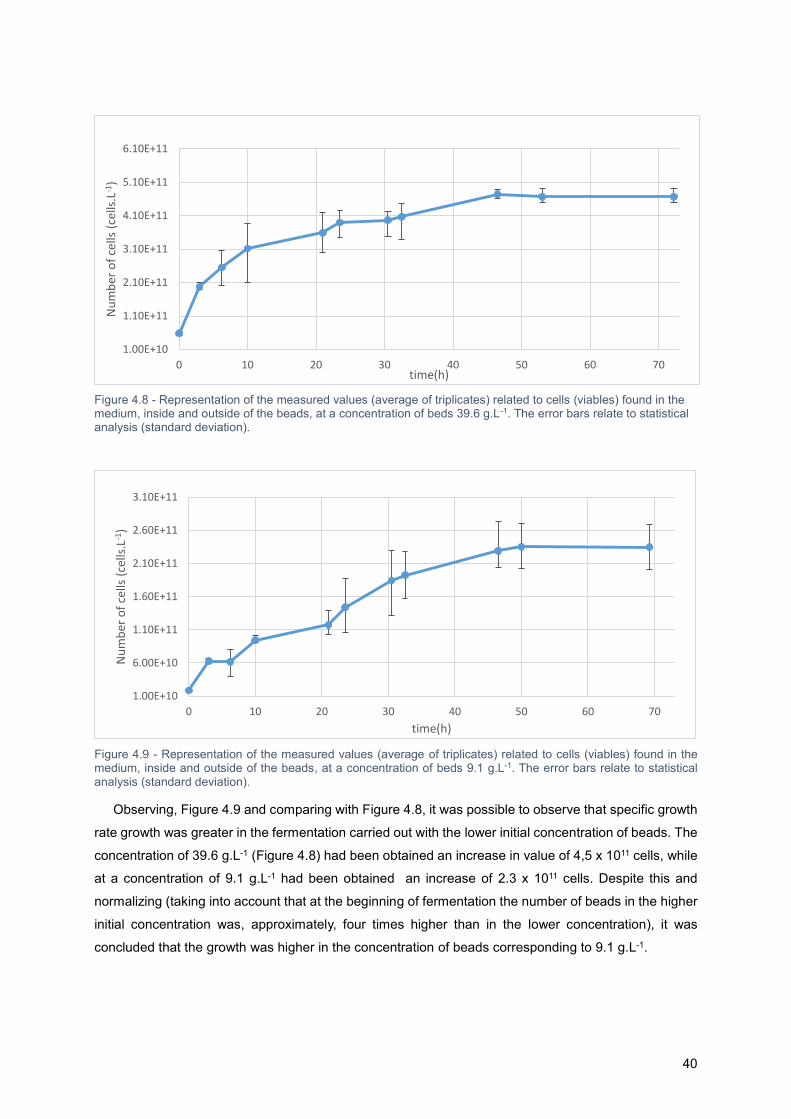
40
Figure 4.8 - Representation of the measured values (average of triplicates) related to cells (viables) found in the medium, inside and outside of the beads, at a concentration of beds 39.6 g.L-1. The error bars relate to statistical analysis (standard deviation).
Figure 4.9 - Representation of the measured values (average of triplicates) related to cells (viables) found in the medium, inside and outside of the beads, at a concentration of beds 9.1 g.L-1. The error bars relate to statistical analysis (standard deviation).
Observing, Figure 4.9 and comparing with Figure 4.8, it was possible to observe that specific growth
rate growth was greater in the fermentation carried out with the lower initial concentration of beads. The
concentration of 39.6 g.L-1 (Figure 4.8) had been obtained an increase in value of 4,5 x 10¹¹ cells, while
at a concentration of 9.1 g.L-1 had been obtained an increase of 2.3 x 10¹¹ cells. Despite this and
normalizing (taking into account that at the beginning of fermentation the number of beads in the higher
initial concentration was, approximately, four times higher than in the lower concentration), it was
concluded that the growth was higher in the concentration of beads corresponding to 9.1 g.L-1.
1.00E+10
1.10E+11
2.10E+11
3.10E+11
4.10E+11
5.10E+11
6.10E+11
0 10 20 30 40 50 60 70
Nu
mb
er o
f ce
lls (
cells
.L-1
)
time(h)
1.00E+10
6.00E+10
1.10E+11
1.60E+11
2.10E+11
2.60E+11
3.10E+11
0 10 20 30 40 50 60 70
Nu
mb
er o
f ce
lls (
cells
.L-1
)
time(h)

41
From Figure 4.8 and Figure 4.9, it is also possible to observe, for both assays (two concentrations),
the variations that exist among the triplicates, which represent the standard deviation (calculated from
triplicates in relation to their average). Comparing the three variables, it is possible to observe that there
are a high standard deviation related to the triplicate measurements of biomass. Therefore, and taking
into account that the original medium and fermentation were the same between triplicates, the
discussion can be brought to the quantification method (technique). The beads referring to the same
concentration, even grown in different Erlenmeyer flasks , presented similar values referring to cell count
(viable and deaths). However, there was a certain disparity in values measured with respect to free cells
released into the fermentation medium, which implies some differentiation between triplicates. One
possible explanation could be related to the sample liquid removed in each measurement (3 mL), which
cannot be uniform among triplicates.
For other measured parameters (substrate and ethanol) the reproducibility of the triplicates was more
exact, as shown in Figure 4.6 and Figure 4.7. Statistical analysis for these variables, as well CO2, is
represented in Annex III - Statistical analysis, where it can be see that the standard deviation and error
is smaller. One explanation for this, it lies in the acquisition of these variables method, HPLC, a high
precision chromatography.
It is also important to highlight the evolution of substrate concentration (obtained through the DNS
method) in order to track the progress of fermentation. As shown in Table 4.4 , it was obtained values of
substrate concentration slightly lower by this method, compared with those obtained by HPLC (these
values can be taken directly from the read of sugars in Figure 4.6 and Figure 4.7). This can be attributed
to the fact that HPLC is a more accurate method in the sense that allow the detection of the pretended
reducing sugars (i.e. glucose and fructose) without being influence by other sugars present in the
medium. On the other hand, DNS technique is not so specific, which means that with this method it is
possible that the measures will not detect only the desired reduced sugar. However, the lower values
obtained with the colorimetric method compared to HPLC can be attributed to the fact that the detection
of the sugars with DNS technique can be influence in a negative way by products/components present
in the medium, leading to an underestimation of the sugars concentration46.
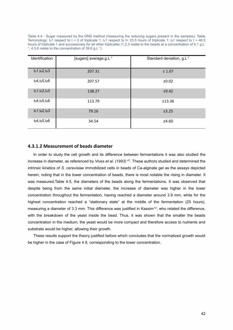
42
Table 4.4 - Sugar measured by the DNS method (measuring the reducing sugars present in the samples). Table Terminology: t01 respect to t = 0 of triplicate 1; t51 respect to t= 23.5 hours of triplicate 1; t81 respect to t = 46.5 hours of triplicate 1 and successively for all other triplicates (1,2,3 relate to the beads at a concentration of 9.1 g.L-
1; 4,5,6 relate to the concentration of 39.6 g.L-1) .
4.3.1.2 Measurement of beads diameter
In order to study the cell growth and its difference between fermentations it was also studied the
increase in diameter, as referenced by Vives et al. (1993) 47. These authors studied and determined the
intrinsic kinetics of S. cerevisiae immobilized cells in beads of Ca-alginate gel as the assays depicted
herein, noting that in the lower concentration of beads, there is most notable the rising in diameter. It
was measured,Table 4.5, the diameters of the beads along the fermentations. It was observed that
despite being from the same initial diameter, the increase of diameter was higher in the lower
concentration throughout the fermentation, having reached a diameter around 3.9 mm, while for the
highest concentration reached a “stationary state” at the middle of the fermentation (25 hours),
measuring a diameter of 3.3 mm. This difference was justified in Kassim12, who related the difference,
with the breakdown of the yeast inside the bead. Thus, it was shown that the smaller the beads
concentration in the medium, the yeast would be more compact and therefore access to nutrients and
substrate would be higher, allowing their growth.
These results support the theory justified before which concludes that the normalized growth would
be higher in the case of Figure 4.9, corresponding to the lower concentration.
Identification [sugars] average,g.L-1 Standard deviation, g.L-1
t01,t02,t03 207.31 ± 1.07
t04,t05,t06 207.57 ±0.02
t51,t52,t53 138.27 ±9.42
t54,t55,t56 113.79 ±13.36
t81,t82,t83 79.16 ±3.25
t84,t85,t86 34.54 ±4.60

43
Table 4.5 - Average diameter (from triplicate) for the two concentrations tested. Values are given in mm (millimetres).
4.3.2. Simulation with new Data (original parameters)
After the treatment and analysis of new data, new simulations were performed in order to study the
correlation between the Model31 with the initial conditions used in the new assays, and experimental
data (new assays). These simulations were made to the two previously referred concentrations, and its
analysis was also made independently in order to take conclusions about the Malherbe et al. (2004)31
model.
Firstly, it was studied the model with experimental results for a concentration of 39.6 g.L-1. It is
recalled that this study had been done in Chapter 4.1, but with data from Kassim12, which appeared to
have some inaccuracies particularly in terms of biomass (biomass has not reached stable values in its
steady state). Observing Figure 4.10, it can be view a good fit between the substrate measured
experimentally and predicted by the model. In consequence, the adjustment for the product is also good.
However in relation to biomass, as can be seen in Figure 4.10, this correlation was not verified: modeled
biomass would reach a maximum around 3 g.L-1, while experimentally there is an increase to about 9
g.L-1, remaining constant after that.
As in the previously referenced Chapter 4.2, it was not obtained a total fit between the data from the
laboratory and the original model proposed by Malherbe et al. (2004)31. Even using the parameters
calculated by the parameter estimation in the previous studies, Table 4.3, the fit would not be achievable.
Thus, it opted for another strategy and directly analyze the model and its structure, as it will be seen
later.
Time ( hours) Bead Diameter,concentration 9.1 g.L-1 Bead Diameter,concentration 39.6 g.L-1
0.00 2.50 2.50
3.00 2.50 2.50
6.25 2.75 2.90
10.0 3.00 3.25
21.0 3.25 3.25
23.5 3.50 3.33
30.5 3.80 3.33
32.5 3.80 3.33
46.5 3.80 3.33
53.0 3.88 3.33
72.3 3.88 3.33

44
Figure 4.10 - New experiments and simulation results made with the original model (original parameters) for a bead concentration of 39.6 g.L-1 in the fermentation medium. Constant Temperature (T) = 20 °C; S0 = 223.5 g.L-1 (average); X0 (real) = 5.76x10⁷ Cellules.mL-1 (1.05 g.L-1); N0=0.385 g.L-1.
It was also studied the fit between the model originally proposed and prepared for further tests on a
concentration of beads 9.1 g.L-1. It can be seen in Figure 4.11 that the differences between the results
proposed by the model and the experimental data were softened. It is verified experimentally that after
about 72 hours (duration of the test fermentation), the substrate reaches values close to 0-1 g.L-1,while
the model predicts that is only reduced to approximately half of the initial substrate, i.e. around 60 g.L-1.
Consequently the adjustment related to the product is also inaccurate. At the level of biomass it was
also found inaccuracies, especially at the stage where there is the passage of cell growth to a steady
state, verifying that experimentally occurs at the beginning of the second day of fermentation, while in
the model occurs after 15 hours in relation to beginning of the fermentation.
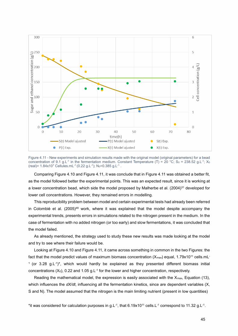
*it was considered for calculation purposes in g.L-1, that 6.19x10¹¹ cells.L-1 correspond to 11.32 g.L-1. 45
Figure 4.11 - New experiments and simulation results made with the original model (original parameters) for a bead concentration of 9.1 g.L-1 in the fermentation medium. Constant Temperature (T) = 20 °C; S0 = 238.52 g.L-1; X0
(real)= 1.84x10⁷ Cellules.mL-1 (0.22 g.L-1); N0=0.385 g.L-1 .
Comparing Figure 4.10 and Figure 4.11, it was conclude that in Figure 4.11 was obtained a better fit,
as the model followed better the experimental points. This was an expected result, since it is working at
a lower concentration bead, which side the model proposed by Malherbe et al. (2004)31 developed for
lower cell concentrations. However, they remained errors in modelling.
This reproducibility problem between model and certain experimental tests had already been referred
in Colombié et al. (2005)48 work, where it was explained that the model despite accompany the
experimental trends, presents errors in simulations related to the nitrogen present in the medium. In the
case of fermentation with no added nitrogen (or too early) and slow fermentations, it was concluded that
the model failed.
As already mentioned, the strategy used to study these new results was made looking at the model
and try to see where their failure would be.
Looking at Figure 4.10 and Figure 4.11, it came across something in common in the two Figures: the
fact that the model predict values of maximum biomass concentration (Xmax) equal, 1.79x10¹¹ cells.mL-
1 (or 3.28 g.L-1)*, which would hardly be explained as they presented different biomass initial
concentrations (X0), 0.22 and 1.05 g.L-1 for the lower and higher concentration, respectively.
Reading the mathematical model, the expression is easily associated with the Xmax, Equation (13),
which influences the dX/dt, influencing all the fermentation kinetics, since are dependent variables (X,
S and N). The model assumed that the nitrogen is the main limiting nutrient (present in low quantities)
46
for cell growth, suggesting a nonlinear function to calculate 𝑋𝑚𝑎𝑥 according with the available assimilable
nitrogen and when it depletes, cell growth ends. However, this model also assumed that a part of the
absorbed nitrogen (during growth) was also directed for the synthesis of sugar transporters, NST. Various
experiments have studied this dual action of the nitrogen in the fermentation, showing that, when the
initial nitrogen is low (less than 100 mg.L-1), yeast focuses primarily on cell growth and production, while
otherwise (abundance of initial nitrogen), cell growth also increases but at the same time more nitrogen
is used for the transporters synthesis (NST), avoiding catabolite inactivation and cell death 49 .
This function, Equation (13), was built for the concentration of biomass (free) tested in the article.
This function took into account only the𝑁𝑖𝑛𝑖𝑡, i.e., if it is applied the same values of 𝛾3, 𝛾4 and 𝛾5 to
different concentrations with the same𝑁𝑖𝑛𝑖𝑡, similar values would be obtained, as those obtained in
Figure 4.8 and Figure 4.9. Nevertheless, as can be concluded, that value depends not only on the initial
nitrogen, but also on 𝑋𝑖𝑛𝑖𝑡. In this way, and once a model is built to be applied in different conditions, this
function had lost its effect in the model. It can be recalculated these parameters (𝛾3, 𝛾4 and 𝛾5) for these
new tests, however it was chosen for future simulations eliminate these parameters of the model,
entering directly 𝑋𝑚𝑎𝑥 value measured experimentally.
Another model “controversy” was the nitrogen, referring to the cells role. In the mode, it was pointed
just as an important factor on cell growth, i.e., its restricted to effect only the exponential part of the
growth. Then, it was also proposed that the nitrogen required for cellular maintenance was also a limiting
factor, and thus could not be negligible 50. This may become an even bigger problem, considering that
the model is constructed on the assumption that the nitrogen is extremely important, i.e., the model is
sensitive to the concentration of assimilable nitrogen48 .
Knowing, a priori from Kassim´s data12, that the prepared medium would contain around 0.385 mg.L-
1 of assimilable nitrogen, it was studied the veracity and evolution of it. First, it was assayed an
experimental method presented in Section 3.2.5, where it is used a ratio between the assimilable
nitrogen and the amount of base added in the titration. However this study proved inconclusive, since
the degree of accuracy did not allow the measurement and monitoring of small amounts nitrogen present
in the samples. It was only demonstrated that nitrogen is rapidly consumed, as expected. It was also
used a correlation presented by Colombiè et al.(2005)48,Equation (22), between the initial assimilable
nitrogen present in the grape juice (or grape must) and the maximum rate of CO2 production (dCO2/dt):
(𝑑𝐶𝑂2
𝑑𝑡)𝑚𝑎𝑥 = −6.76𝑥10−6(𝑁𝑖𝑛𝑖𝑡)2 + 8.50𝑥10−3(𝑁𝑖𝑛𝑖𝑡) − 3.59𝑥10−2
(22)
In the laboratory, the release of CO2 was controlled, as mentioned in the Section 3.2.1. By constant
measurement of weight loss it was constructed in the following Table 4.6:

47
Table 4.6 - Representative dCO2/dt over 72.25 hours of fermentation for each one of tested concentrations. In bold are indicated the (dCO2/dt)max .
Applying the maximum detected values in Equation (22), it was obtained the values for initial
concentrations of assimilable nitrogen, 263.42 and 421.09 g.L-1. These values can be proven through
the parable48 represented in Annex V.
This difference between estimated values for the initial nitrogen was not in agreement with the
expected, since both tests were prepared from the same fermentation medium, then the values have to
be similar. Once the value obtained from the tests with the lowest concentration was below the
expectations, it was decided to simulate the amount corresponding to 421.09 g.L-1.
4.3.3. Simulation with new Data (new approach)
With the conclusions drawn from section 4.3.2, it was performed new simulations with the changes
highlighted in the model and in respect to the amount of initial assimilable nitrogen. It was also made a
parametric estimation on the level of parameter k2 (T) for the lower concentration, due to the oscillation
previously observed in the values compared with the originally proposed (Table 4.3). The results can be
seen in Figure 4.12 and Figure 4.13.
Time ( hours) (𝒅𝑪𝑶𝟐
𝒅𝒕)𝒎𝒂𝒙, 9.1 g.L-1 (
𝒅𝑪𝑶𝟐
𝒅𝒕)𝒎𝒂𝒙, 39.6 g.L-1
0.00 0 0
3.00 0.32 0.48
6.25 0.43 0.95
10.0 0.37 1.51
21.0 1.15 2.34
23.5 1.21 1.83
30.5 1.73 2.28
32.5 1.70 2.50
46.5 1.36 1.88
53 1.28 1.66
72.3 1.29 0.66
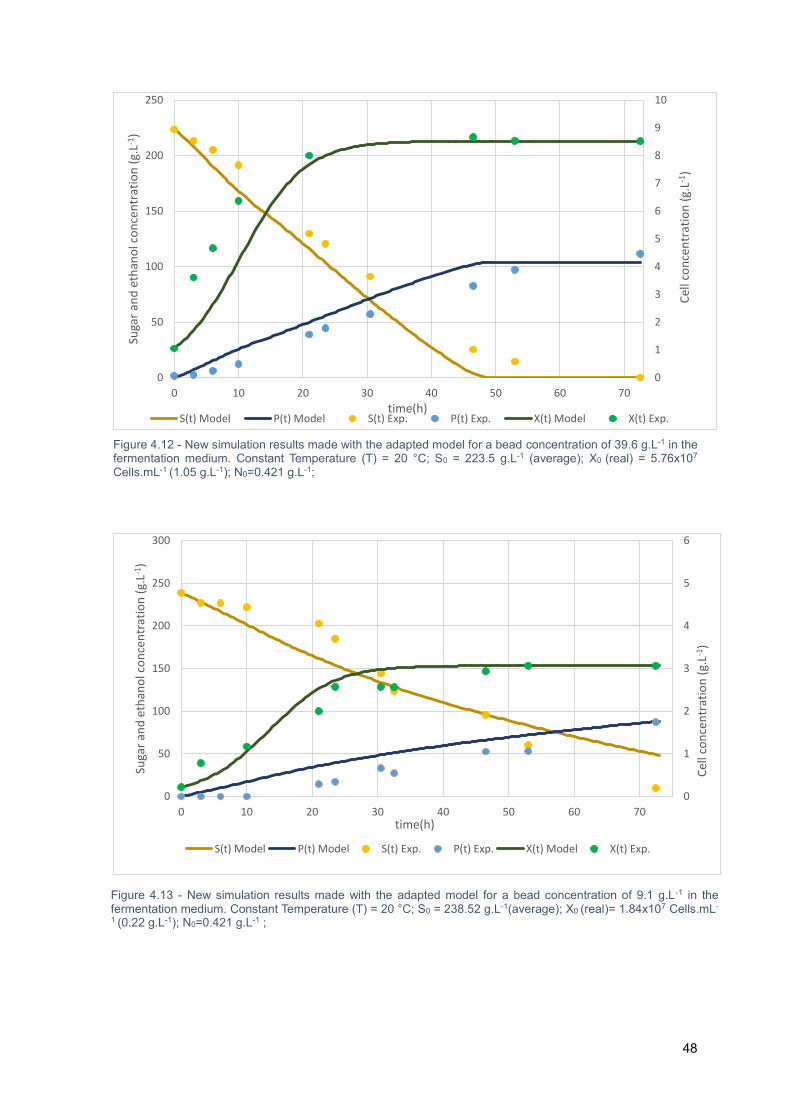
48
Figure 4.12 - New simulation results made with the adapted model for a bead concentration of 39.6 g.L-1 in the fermentation medium. Constant Temperature (T) = 20 °C; S0 = 223.5 g.L-1 (average); X0 (real) = 5.76x10⁷ Cells.mL-1 (1.05 g.L-1); N0=0.421 g.L-1;
0
1
2
3
4
5
6
7
8
9
10
0
50
100
150
200
250
0 10 20 30 40 50 60 70
Cel
l co
nce
ntr
atio
n (
g.L-1
)
Suga
r an
d e
than
ol c
on
cen
trat
ion
(g.
L-1)
time(h)S(t) Model P(t) Model S(t) Exp. P(t) Exp. X(t) Model X(t) Exp.
0
1
2
3
4
5
6
0
50
100
150
200
250
300
0 10 20 30 40 50 60 70
Cel
l co
nce
ntr
atio
n (
g.L-1
)
Suga
r an
d e
than
ol c
on
cen
trat
ion
(g.
L-1)
time(h)
S(t) Model P(t) Model S(t) Exp. P(t) Exp. X(t) Model X(t) Exp.
Figure 4.13 - New simulation results made with the adapted model for a bead concentration of 9.1 g.L-1 in the fermentation medium. Constant Temperature (T) = 20 °C; S0 = 238.52 g.L-1(average); X0 (real)= 1.84x10⁷ Cells.mL-
1 (0.22 g.L-1); N0=0.421 g.L-1 ;
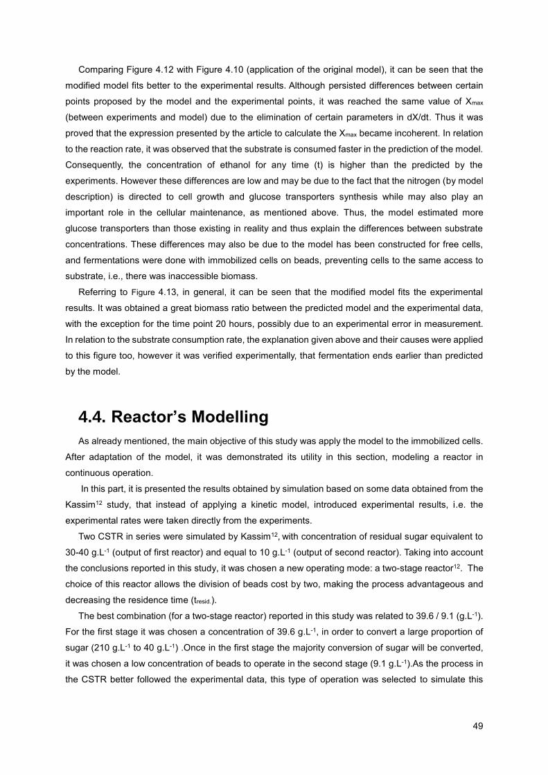
49
Comparing Figure 4.12 with Figure 4.10 (application of the original model), it can be seen that the
modified model fits better to the experimental results. Although persisted differences between certain
points proposed by the model and the experimental points, it was reached the same value of Xmax
(between experiments and model) due to the elimination of certain parameters in dX/dt. Thus it was
proved that the expression presented by the article to calculate the Xmax became incoherent. In relation
to the reaction rate, it was observed that the substrate is consumed faster in the prediction of the model.
Consequently, the concentration of ethanol for any time (t) is higher than the predicted by the
experiments. However these differences are low and may be due to the fact that the nitrogen (by model
description) is directed to cell growth and glucose transporters synthesis while may also play an
important role in the cellular maintenance, as mentioned above. Thus, the model estimated more
glucose transporters than those existing in reality and thus explain the differences between substrate
concentrations. These differences may also be due to the model has been constructed for free cells,
and fermentations were done with immobilized cells on beads, preventing cells to the same access to
substrate, i.e., there was inaccessible biomass.
Referring to Figure 4.13, in general, it can be seen that the modified model fits the experimental
results. It was obtained a great biomass ratio between the predicted model and the experimental data,
with the exception for the time point 20 hours, possibly due to an experimental error in measurement.
In relation to the substrate consumption rate, the explanation given above and their causes were applied
to this figure too, however it was verified experimentally, that fermentation ends earlier than predicted
by the model.
4.4. Reactor’s Modelling
As already mentioned, the main objective of this study was apply the model to the immobilized cells.
After adaptation of the model, it was demonstrated its utility in this section, modeling a reactor in
continuous operation.
In this part, it is presented the results obtained by simulation based on some data obtained from the
Kassim12 study, that instead of applying a kinetic model, introduced experimental results, i.e. the
experimental rates were taken directly from the experiments.
Two CSTR in series were simulated by Kassim12, with concentration of residual sugar equivalent to
30-40 g.L-1 (output of first reactor) and equal to 10 g.L-1 (output of second reactor). Taking into account
the conclusions reported in this study, it was chosen a new operating mode: a two-stage reactor12. The
choice of this reactor allows the division of beads cost by two, making the process advantageous and
decreasing the residence time (tresid.).
The best combination (for a two-stage reactor) reported in this study was related to 39.6 / 9.1 (g.L-1).
For the first stage it was chosen a concentration of 39.6 g.L-1, in order to convert a large proportion of
sugar (210 g.L-1 to 40 g.L-1) .Once in the first stage the majority conversion of sugar will be converted,
it was chosen a low concentration of beads to operate in the second stage (9.1 g.L-1).As the process in
the CSTR better followed the experimental data, this type of operation was selected to simulate this

50
operation. Some operating parameters were found in Kassim12 study and set a priori of simulation, such
as Q, C0 and Cf. Results of this simulation are shown in the following Table 4.7.
Table 4.7 - Simulation results in CSTR for a two stage reactor. Operating parameters such as Q, C0, Cf were taken directly from Kassim12 study. The remaining parameters were calculated. As a reference for the beads, it was admitted that 60.5 grams of dried beads were equivalent to a volume of 170 mL (when rehydrated). tresid=(Cf-C0)/(rateconsum.sugars)
It was calculated a global volume (in this case for 2 stirred reactors) of 6479 x 103 L, above
expectations from the results of Kassim12, 4781 x 103 L. It was obtained a residence time of 69 hours.
These differences between values were lied to the substrate consumption rate on the second stage
(referring to the concentration of 9.1 g.L-1), which was observable in Figure 4.13 (it can be seen a slowly
rate when the substrates crossed 10 g.L-1 of available). Thus, despite the second floor had been a
residual concentration, the utilisation of this low concentration increased the residence time of the
fermentation. For example, in the case of keeping the concentration of 39.6 g.L-1 to the second floor,
with a substrate consumption rate around 3.5 g.L-1.h-1, the total system volume was reduced to 4375.9
x 103 L (and the residence time to 46 hours).
Assuming a unit cost of 50 €. (Kg of beads)-1, it is understood that this choice of beads concentrations
must be target of a study of cost/benefit. By increasing the concentration of beads, increases up the
tank volume (in this case column) and thus enhances the cost associated with the equipment. However,
the substrate consumption rate also decreases, which is reflected negatively in the residence time (tresid.).
Stage 1st Stage 2nd Stage
Concentration of beads in
the medium (g.L-1)
39.6 9.1
Q (L.h-1) 8929 8929
C0 (g.L-1) 210 40
Cf (g.L-1) 40 10
Sugars Consumation rate
(gsugars.L-1.h-1)
4.5 0.9
tresid.(h) 37.5 31.7
D (h-1) 0.026 0.031
vliq (L.103) 3347.8 2832.81
mbeads (kg) 13257.2 2577.8
vbeads (L.103) 249.6 48.5
51
5. Conclusion and future perspectives
This project aimed to apply a kinetic model, originally developed for a system with free yeast cells,
in order to follow alcoholic fermentation with immobilized cells. To this end, simulations were performed
in some computing environments in order to realize this optimization. Thus, it was first used data already
set for the conditions of the work. They were made several parametric estimates, however the data
contained some inconsistencies within the biomass. It was performed new fermentations, where once
again it was found that the model did not fit the experimental results. Once this work was done with
immobilized cells, the most plausible explanation would be a conditioning phenomenon on the level of
mass transfer. However, it is known that this problem is minimized by using the support made of calcium
alginate, which maximizes the number of cells within their beads51. The strategy adopted was inherently
study the mathematical model and it was found a few fails. In terms of biomass, came across Xmax
calculation was not valid for high concentrations of initial biomass, being eliminated the parameters
of 𝛾3, 𝛾4 and 𝛾5. Moreover, the experimental results showed that the contribution of nitrogen for cellular
maintenance was not negligible, as the model assumed50. In addition to these variables that were
corrected through the experiences, the parameter estimation and optimization returned a new value of
k2. In the end, with changes made to Malherbe31 model, it was obtained a good correlation between the
predicted mathematically and the results of fermentation. It is concluded that the model was feasible to
design a continuous system. Its applicability was demonstrated in a two stage-reactor, reaching a
residence time of 69 hours.
In the future, some changes to the model can also be applied, especially regarding nitrogen (dN /dt),
which can be added an expression which takes into account the nitrogen used to cellular maintenance
(Monod kinetics for example). The study of continuous fermentation can also be extended, and launched
the system provided by the simulation done in this work.
52
6. References
1. Maxon WD. Continuous Fermentation: A Discussion of Its Pinciples and Applications. Microbiol Process Rep. 1955;3(2):12.
2. Calvet J. Nature and Problems of French Wine Clusters. :1-26.
3. Genisheva Z, Teixeira J., Oliveira JM. Immobilized cell systems for batch and continuous winemaking. Trends Food Sci Technol. 2014;40(1):33-47. doi:10.1016/j.tifs.2014.07.009.
4. Guo X, Li H, Xu H, et al. Glycolysis in the control of blood glucose homeostasis. Acta Pharm Sin B. 2012;2(4):358-367. doi:10.1016/j.apsb.2012.06.002.
5. Jolly NP, Augustyn OPH, Pretorius IS. The Role and Use of Non-Saccharomyces Yeasts in Wine Production. South African J Enol Vitic. 2006;27(1):15-39.
6. Bakker BM, Bro C, Kotter P, Luttik M a H, Van Dijken JP, Pronk JT. The mitochondrial alcohol dehydrogenase ADH3p is involved in a redox shuttle in Saccharomyces cerevisiae. J Bacteriol. 2000;182(17):4730-4737. doi:10.1128/JB.182.17.4730-4737.2000.
7. van Maris AJA, Abbott DA, Bellissimi E. Alcoholic fermentation of carbon sources in biomass hydrolysates by Saccharomyces cerevisiae: current status. Antonie Van Leeuwenhoek. 2006;90(4):391-418. doi:10.1007/s10482-006-9085-7.
8. Silva-Graça M, Lucas C. Physiological studies on long-term adaptation to salt stress in the extremely halotolerant yeast Candida versatilis CBS 4019 (syn. C. halophila ). FEMS Yeast Res. 2003;3(3):247-260. doi:10.1111/j.1567-1364.2003.tb00167.x.
9. Bai FW, Anderson WA, Moo-Young M. Ethanol fermentation technologies from sugar and starch feedstocks. Biotechnol Adv. 2008;26(1):89-105. doi:10.1016/j.biotechadv.2007.09.002.
10. Wanke H, Bruckner J, Dreibus G, Rieder R, Ryabchikov I. Chemical composition of rocks and soils at the Pathfinder site. Space Sci Rev. 2001;96(October):317-330. doi:10.1023/A.
11. Wu R, Racker E. Regulatory Mechanisms in Carbohydrate Metabolism. IV. Pasteur Effect and Crabtree effect in ascites tumor cells. J Biol Chem. 1959;234(5):1036-1041. http://www.jbc.org/content/234/5/1036.short. Accessed November 1, 2015.
12. Kassim C. Vinification continue avec levures immobilisées : analyse du système et conception du réacteur industriel.February 2012. http://ethesis.inp-toulouse.fr/archive/00001833/. Accessed October 28, 2015.

53
13. Kourkoutas Y, Koutinas AA , Kanellaki M, Banat IM, Marchant R. Continuous wine fermentation using a psychrophilic yeast immobilized on apple cuts at different temperatures. Food Microbiol. 2002;19(2-3):127-134. doi:10.1006/fmic.2001.0468.
14. Pretorius IS. Tailoring wine yeast for the new millennium: novel approaches to the ancient art of winemaking. Yeast. 2000;16(8):675-729. doi:10.1002/1097-0061(20000615)16:8<675::AID-YEA585>3.0.CO;2-B.
15. Rainieri S, Pretorius I. Selection and improvement of wine yeasts. Ann Microbiol. 2000;50(October):15-31.
16. Manzano M, Medrala D, Giusto C, Bartolomeoli I, Urso R, Comi G. Classical and molecular analyses to characterize commercial dry yeasts used in wine fermentations. J Appl Microbiol. 2006;100(3):599-607. doi:10.1111/j.1365-2672.2005.02807.x.
17. Fleet GH. Wine yeasts for the future. FEMS Yeast Res. 2008;8(7):979-995. doi:10.1111/j.1567-1364.2008.00427.x.
18. Cantarelli C, Lanzarini G, eds. Biotechnology Applications in Beverage Production. Dordrecht: Springer Netherlands; 1989. doi:10.1007/978-94-009-1113-0.
19. Pilkington PH, Margaritis A, Mensour NA, Russell I. Fundamentals of immobilised yeast cells for continuous beer fermentation: a review. J Inst Brew. 1998;104(1):19-31. doi:10.1002/j.2050-0416.1998.tb00970.x.
20. Verbelen PJ, De Schutter DP, Delvaux F, Verstrepen KJ, Delvaux FR. Immobilized yeast cell systems for continuous fermentation applications. Biotechnol Lett. 2006;28(19):1515-1525. doi:10.1007/s10529-006-9132-5.
21. Eroglu S., Toprak S., Urgan O, Ozge E. Onur, Arzu Denizbasi, Haldun Akoglu, Cigdem Ozpolat, Ebru Akoglu M. Yeasts in Food and Beverages. Saudi Med J. 2012;33:3-8. doi:10.1073/pnas.0703993104.
22. Kassim C, Alliet M, Favarel JL, Taillandier P, Strehaiano P. Mise au point d’un réacteur de vinification en continu sur un mélange S . Cerevisiae et Sch . pombe immobilisées dans de l ’ alginate de calcium . 2011:6-11.
23. Kierstan M, Bucke C. The immobilization of microbial cells, subcellular organelles, and enzymes in calcium alginate gels. Biotechnol Bioeng. 1977;19(3):387-397. doi:10.1002/bit.260190309.
24. Jirku V. Whole cell immobilization as a means of enhancing ethanol tolerance. J Ind Microbiol Biotechnol. 1999;22(3):147-151. doi:10.1038/sj.jim.2900620.
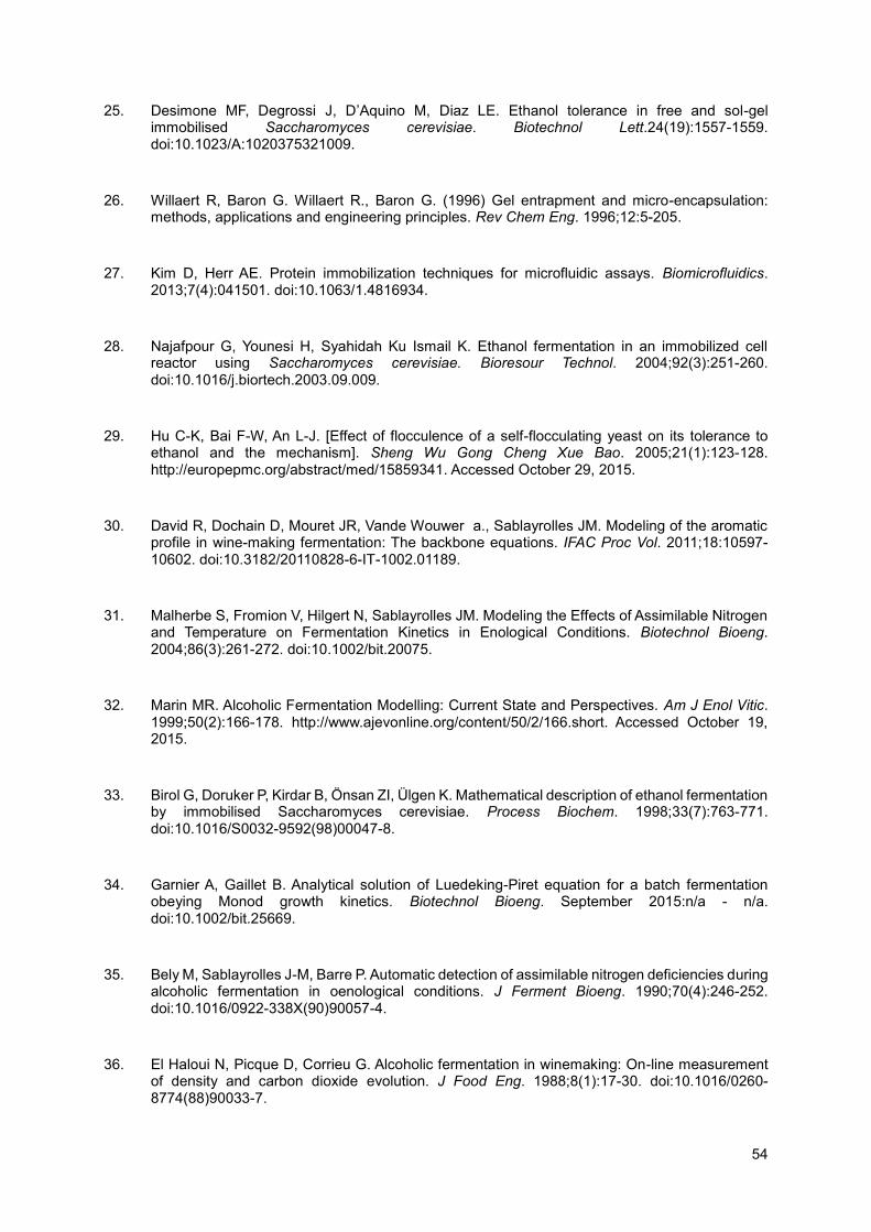
54
25. Desimone MF, Degrossi J, D’Aquino M, Diaz LE. Ethanol tolerance in free and sol-gel immobilised Saccharomyces cerevisiae. Biotechnol Lett.24(19):1557-1559. doi:10.1023/A:1020375321009.
26. Willaert R, Baron G. Willaert R., Baron G. (1996) Gel entrapment and micro-encapsulation: methods, applications and engineering principles. Rev Chem Eng. 1996;12:5-205.
27. Kim D, Herr AE. Protein immobilization techniques for microfluidic assays. Biomicrofluidics. 2013;7(4):041501. doi:10.1063/1.4816934.
28. Najafpour G, Younesi H, Syahidah Ku Ismail K. Ethanol fermentation in an immobilized cell reactor using Saccharomyces cerevisiae. Bioresour Technol. 2004;92(3):251-260. doi:10.1016/j.biortech.2003.09.009.
29. Hu C-K, Bai F-W, An L-J. [Effect of flocculence of a self-flocculating yeast on its tolerance to ethanol and the mechanism]. Sheng Wu Gong Cheng Xue Bao. 2005;21(1):123-128. http://europepmc.org/abstract/med/15859341. Accessed October 29, 2015.
30. David R, Dochain D, Mouret JR, Vande Wouwer a., Sablayrolles JM. Modeling of the aromatic profile in wine-making fermentation: The backbone equations. IFAC Proc Vol. 2011;18:10597-10602. doi:10.3182/20110828-6-IT-1002.01189.
31. Malherbe S, Fromion V, Hilgert N, Sablayrolles JM. Modeling the Effects of Assimilable Nitrogen and Temperature on Fermentation Kinetics in Enological Conditions. Biotechnol Bioeng. 2004;86(3):261-272. doi:10.1002/bit.20075.
32. Marin MR. Alcoholic Fermentation Modelling: Current State and Perspectives. Am J Enol Vitic. 1999;50(2):166-178. http://www.ajevonline.org/content/50/2/166.short. Accessed October 19, 2015.
33. Birol G, Doruker P, Kirdar B, Önsan ZI, Ülgen K. Mathematical description of ethanol fermentation by immobilised Saccharomyces cerevisiae. Process Biochem. 1998;33(7):763-771. doi:10.1016/S0032-9592(98)00047-8.
34. Garnier A, Gaillet B. Analytical solution of Luedeking-Piret equation for a batch fermentation obeying Monod growth kinetics. Biotechnol Bioeng. September 2015:n/a - n/a. doi:10.1002/bit.25669.
35. Bely M, Sablayrolles J-M, Barre P. Automatic detection of assimilable nitrogen deficiencies during alcoholic fermentation in oenological conditions. J Ferment Bioeng. 1990;70(4):246-252. doi:10.1016/0922-338X(90)90057-4.
36. El Haloui N, Picque D, Corrieu G. Alcoholic fermentation in winemaking: On-line measurement of density and carbon dioxide evolution. J Food Eng. 1988;8(1):17-30. doi:10.1016/0260-8774(88)90033-7.
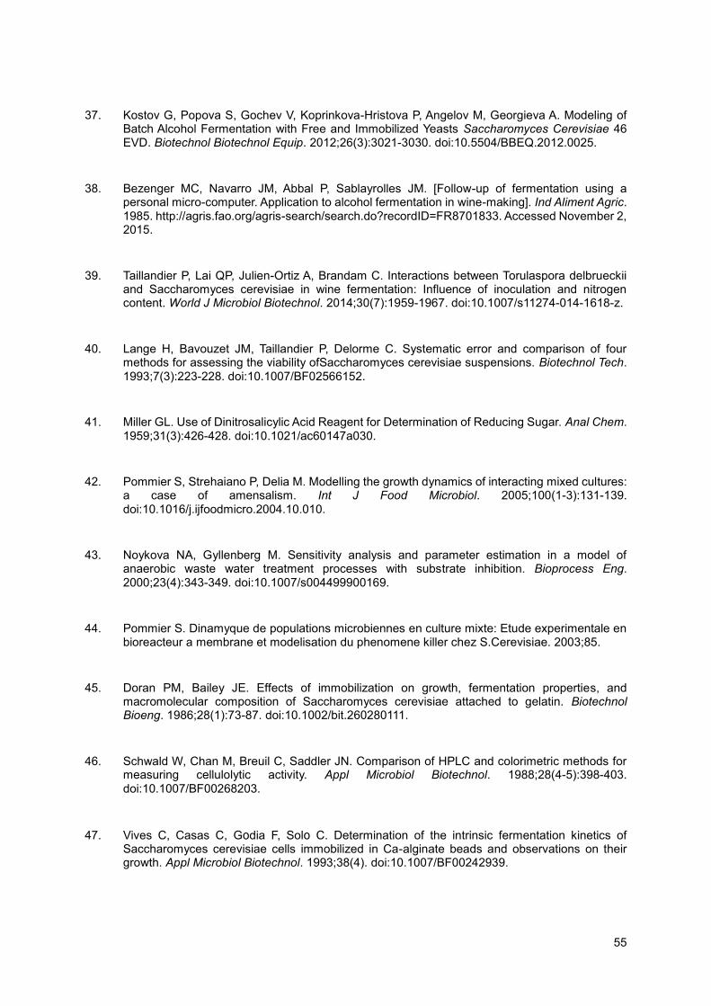
55
37. Kostov G, Popova S, Gochev V, Koprinkova-Hristova P, Angelov M, Georgieva A. Modeling of Batch Alcohol Fermentation with Free and Immobilized Yeasts Saccharomyces Cerevisiae 46 EVD. Biotechnol Biotechnol Equip. 2012;26(3):3021-3030. doi:10.5504/BBEQ.2012.0025.
38. Bezenger MC, Navarro JM, Abbal P, Sablayrolles JM. [Follow-up of fermentation using a personal micro-computer. Application to alcohol fermentation in wine-making]. Ind Aliment Agric. 1985. http://agris.fao.org/agris-search/search.do?recordID=FR8701833. Accessed November 2, 2015.
39. Taillandier P, Lai QP, Julien-Ortiz A, Brandam C. Interactions between Torulaspora delbrueckii and Saccharomyces cerevisiae in wine fermentation: Influence of inoculation and nitrogen content. World J Microbiol Biotechnol. 2014;30(7):1959-1967. doi:10.1007/s11274-014-1618-z.
40. Lange H, Bavouzet JM, Taillandier P, Delorme C. Systematic error and comparison of four methods for assessing the viability ofSaccharomyces cerevisiae suspensions. Biotechnol Tech. 1993;7(3):223-228. doi:10.1007/BF02566152.
41. Miller GL. Use of Dinitrosalicylic Acid Reagent for Determination of Reducing Sugar. Anal Chem. 1959;31(3):426-428. doi:10.1021/ac60147a030.
42. Pommier S, Strehaiano P, Delia M. Modelling the growth dynamics of interacting mixed cultures: a case of amensalism. Int J Food Microbiol. 2005;100(1-3):131-139. doi:10.1016/j.ijfoodmicro.2004.10.010.
43. Noykova NA, Gyllenberg M. Sensitivity analysis and parameter estimation in a model of anaerobic waste water treatment processes with substrate inhibition. Bioprocess Eng. 2000;23(4):343-349. doi:10.1007/s004499900169.
44. Pommier S. Dinamyque de populations microbiennes en culture mixte: Etude experimentale en bioreacteur a membrane et modelisation du phenomene killer chez S.Cerevisiae. 2003;85.
45. Doran PM, Bailey JE. Effects of immobilization on growth, fermentation properties, and macromolecular composition of Saccharomyces cerevisiae attached to gelatin. Biotechnol Bioeng. 1986;28(1):73-87. doi:10.1002/bit.260280111.
46. Schwald W, Chan M, Breuil C, Saddler JN. Comparison of HPLC and colorimetric methods for measuring cellulolytic activity. Appl Microbiol Biotechnol. 1988;28(4-5):398-403. doi:10.1007/BF00268203.
47. Vives C, Casas C, Godia F, Solo C. Determination of the intrinsic fermentation kinetics of Saccharomyces cerevisiae cells immobilized in Ca-alginate beads and observations on their growth. Appl Microbiol Biotechnol. 1993;38(4). doi:10.1007/BF00242939.

56
48. Colombié S, Malherbe S, Sablayrolles JM. Modeling alcoholic fermentation in enological conditions: Feasibility and interest. Am J Enol Vitic. 2005;56(3):238-245.
49. David R, Dochain D, Mouret JR, Vande Wouwer A., Sablayrolles JM. Dynamical modeling of alcoholic fermentation and its link with nitrogen consumption. IFAC Proc Vol. 2010;11(PART 1):496-501. doi:10.3182/20100707-3-BE-2012.0095.
50. Tauro P, Kapoor KK, Yadav KS. An Introduction to Microbiology. New Age International; 1986. https://books.google.com/books?id=xU85I7R-kFsC&pgis=1. Accessed November 15, 2015.
51. Margaritis A, Bajpai PK, Wallace JB. High ethanol productivities using small Ca-alginate beads of immobilized cells of Zymomonas mobilis. Biotechnol Lett. 1981;3(11):613-618. doi:10.1007/BF00158688.
I
7. Annexes
Annex I - Yeast Information
Figure 7.1 – Some information about immobilized yeast cells, ProRestart® (Proenol , Biotech Company)
II
Annex II- HPLC Curves Calibration
Figure 7.2 - Calibration curve for ethanol and the corresponding equation.
Figure 7.3 - Calibration curve for glucose and the corresponding equation.
Figure 7.4 - Calibration curve for fructose and the corresponding equation.
y = 1E+07x + 4E+06R² = 0.9959
0.00E+00
2.00E+07
4.00E+07
6.00E+07
8.00E+07
1.00E+08
1.20E+08
0 2 4 6 8 10 12
Ab
sorb
ance
(5
40
nm
)
Concentration (g.L-1)
y = 4E+06x + 1E+06R² = 0.9961
0.00E+00
1.00E+07
2.00E+07
3.00E+07
4.00E+07
5.00E+07
0 2 4 6 8 10 12
Ab
sorb
ance
(5
40
nm
)
Concentration (g.L-1)
y = 1E+07x + 5E+06R² = 0.9958
0.00E+00
2.00E+07
4.00E+07
6.00E+07
8.00E+07
1.00E+08
1.20E+08
1.40E+08
0 2 4 6 8 10 12
Ab
sorb
ance
(5
40
nm
)
Concentration (g.L-1)

III
Annex III - Statistical analysis
Concentration of 9.1 g.L1
Figure 7.5 - Representation of the measured values (average of triplicates) related to reducing sugars
present in the medium, at a concentration of beds 9.1 g.L-1. The error bars relate to statistical analysis (standard deviation).
Figure 7.6 - Representation of the measured values (average of triplicates) related to ethanol present in the medium, at a concentration of beds 9.1 g.L-1. The error bars relate to statistical analysis (standard deviation).
0
50
100
150
200
250
0 10 20 30 40 50 60 70
Suga
r co
cen
trat
ion
(g/
L)
time(h)
0
20
40
60
80
100
0 10 20 30 40 50 60 70
Eth
ano
l co
nce
ntr
atio
n (
g/L)
time(h)
0
20
40
60
80
100
0 10 20 30 40 50 60 70
CO
2co
nce
ntr
atio
n (
g/L)
time(h)
Figure 7.7 - Representation of the measured values (average of triplicates) related to CO2 released
during the fermentation, at a concentration of beds 9.1 g.L-1. The error bars relate to statistical analysis (standard deviation).
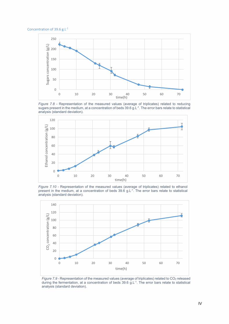
IV
Concentration of 39.6 g.L-1
0
50
100
150
200
250
0 10 20 30 40 50 60 70
Suga
rs c
on
cen
trat
ion
(g/
L)
time(h)
Figure 7.8 - Representation of the measured values (average of triplicates) related to reducing sugars present in the medium, at a concentration of beds 39.6 g.L-1. The error bars relate to statistical analysis (standard deviation).
0
20
40
60
80
100
120
0 10 20 30 40 50 60 70
Eth
ano
l co
nce
ntr
atio
n (
g/L)
time(h)
Figure 7.10 - Representation of the measured values (average of triplicates) related to ethanol present in the medium, at a concentration of beds 39.6 g.L-1. The error bars relate to statistical analysis (standard deviation).
0
20
40
60
80
100
120
140
0 10 20 30 40 50 60 70
CO
2co
nce
ntr
atio
n (
g/L)
time(h)
Figure 7.9 - Representation of the measured values (average of triplicates) related to CO2 released during the fermentation, at a concentration of beds 39.6 g.L-1. The error bars relate to statistical analysis (standard deviation).
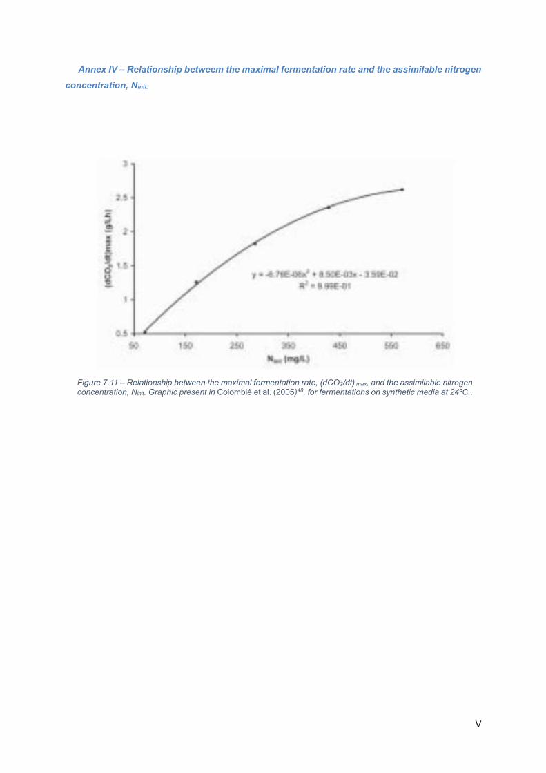
V
Annex IV – Relationship betweem the maximal fermentation rate and the assimilable nitrogen
concentration, Ninit.
Figure 7.11 – Relationship between the maximal fermentation rate, (dCO2/dt) max, and the assimilable nitrogen concentration, Ninit. Graphic present in Colombié et al. (2005)48, for fermentations on synthetic media at 24ºC..