development of univariate control chart for non normal data
TRANSCRIPT
8/22/2019 Development of Univariate Control Chart for Non Normal Data
http://slidepdf.com/reader/full/development-of-univariate-control-chart-for-non-normal-data 1/87
DEVELOPMENT OF UNIVARIATE CONTROL
CHARTS FOR NON-NORMAL DATA
A Thesis Submitted to theGraduate School of Engineering and Sciences of
İzmir Institute of TechnologyIn Partial Fullfilment of the Requirements for the Degree of
MASTER OF SCIENCE
in Materials Science and Engineering
By
Cihan ÇİFLİKLİ
December 2006
İZMİR

8/22/2019 Development of Univariate Control Chart for Non Normal Data
http://slidepdf.com/reader/full/development-of-univariate-control-chart-for-non-normal-data 2/87
ii
We approve the thesis of Cihan ÇİFLİKLİ
Date of Signature
………………………………… 4 December 2006Assist. Prof. Dr. Fuat DOYMAZSupervisor
Department of Chemical Engineering
İzmir Institute of Technology
………………………………… 4 December 2006
Assoc. Prof. Dr. Sedat AKKURTCo-Supervisor
Department of Materials Science and Engineeringİzmir Institute of Technology
………………………………… 4 December 2006
Prof. Dr. Halis PÜSKÜLCÜDepartment of Computer Engineering
İzmir Institute of Technology
………………………………… 4 December 2006
Prof. Dr. Mehmet POLATDepartment of Chemical Engineering
İzmir Institute of Technology
………………………………… 4 December 2006
Assist. Prof. Dr. Mustafa ALTINKAYADepartment of Electrical and Elektronics Engineering
İzmir Institute of Technology
………………………………… 4 December 2006
Prof. Dr. Muhsin ÇİFTÇİOĞLUHead of Department of Materials Science and Engineering
İzmir Institute of Technology
…………………………
Head of the Graduate School

8/22/2019 Development of Univariate Control Chart for Non Normal Data
http://slidepdf.com/reader/full/development-of-univariate-control-chart-for-non-normal-data 3/87
iii
ACKNOWLEDGEMENT
I would like to express my sincere gratitude to my advisor Assist. Prof. Dr. Fuat
Doymaz and co-advisor Assoc. Prof. Dr. Sedat Akkurt for their supervision, guidance
and generosity in sharing their expertise.
I would like to appreciate Prof. Dr. Muhsin Çiftçioğlu, Prof. Dr. Halis Püskülcü,
Prof. Dr. Mehmet Polat, Assist.Prof. Dr. Mustafa Altınkaya and Assist.Prof. Dr. Figen
Tokatlı for their understanding, support and encouragement.
I am thankful to Çimentaş A.Ş. and Burak Akyol for their support.
Special thanks to Levent Aydın, İlker Polatoğlu, Hakk ı Erhan Sevil, Filiz Yaşar
and all my friends for their friendship, help and understanding.
Finally, I want to express my gratitude to my family who made it possible to
overcome all the obstacles I have come across throughout this work.

8/22/2019 Development of Univariate Control Chart for Non Normal Data
http://slidepdf.com/reader/full/development-of-univariate-control-chart-for-non-normal-data 4/87
iv
ABSTRACT
DEVELOPMENT OF UNIVARIATE CONTROL CHARTS FOR NON-
NORMAL DATA
In this study, a new control chart methodology was developed to address
statistical process monitoring issue associated with non-normally distributed process
variables. The new method (NM) was compared aginst the classical Shewhart control
chart (OM) using synthetic datasets from normal and non-normal distributions as well
as over an industrial example. The NM involved taking the difference between the
specified probability density estimate and non-parametric density estimate of the
variable of interest to calculate an error value. Both OM and NM were found to work
well for normally distributed data when process is in-control and out-of control
situation. Both methods could be returned back to normal operation upon feeding in-
control data.
In case of non-normally distributed data, the OM failed significantly to detect
small shifts in mean and standard deviation, however the NM maintained its
performance to detect such changes.
In the application to an industrial case (data were obtained from a local cement
manufacturer about a 90 micrometer sieve fraction of the final milled cement product),
the NM methodology outperformed the OM by recognizing the change in the mean and
variance of the measured parameter. The data were tested for its distribution and were
found to be non-normally distributed. Violations beyond the control limits in the new
developed technique were easily observed. The NM was found to successfully operate
without the necessity to apply run rules.

8/22/2019 Development of Univariate Control Chart for Non Normal Data
http://slidepdf.com/reader/full/development-of-univariate-control-chart-for-non-normal-data 5/87
v
ÖZET
NORMAL DAĞILIMA SAHİP OLMAYAN DEĞİŞKENLER İÇİ N
KONTROL GRAFİKLER İ Nİ N GELİŞTİR İLMESİ
Bu çalışmada, normal olarak dağılmayan proses değişkenleri ile ilintili
istatistiksel proses gözleme amacına cevap verecek yeni bir kontrol grafiği metodolojisi
geliştirilmiştir. Rastgele normal, normal olmayan dağılımlara sahip olan ve sanayi veri
kümelerine Shewhart kontrol grafiklerinin (EY) uygulanması ve bunlar ın yeni yöntem
(YY) ile k ıyaslanması yapılmıştır. YY bir hata değeri hesaplamak için, ilgili değişkenin
parametrik olmayan yoğunluk tahmini değerinin ve belirlenen ihtimal yoğunluğu
tahmininin arasındaki fark ın bulunmasını kapsar. Normal dağılmış verinin kontrol
altında ve kontrol dışındaki durumlar ı için EY ve YY yöntemlerinin her ikisinin de iyi
çalıştığı gözlendi. Kontrol sınırlar ı içinde veri beslenince her iki yöntemin de normal
operasyona döndürülebildiği gösterildi.
Normal dağılmayan veri durumunda ise, EY ortalama ve standard sapmadaki
küçük değişiklikleri yakalamada başar ısız olurken YY bu değişiklikleri yakalamada
başar ılı oldu.
YY’in çimento üreticisinden temin edilen ve 90 mikron elek üstü öğütülmüş
çimento miktar ını (DACK 90) içeren sanayi verilerine uygulanması durumunda EY’e
göre ölçülen parametrenin ortalaması ve varyansındaki değişiklikleri tanımada daha
başar ılı olduğu tespit edildi. Verinin dağılımı sınandı ve normal olmayan şekilde
dağıldığı tespit edildi. YY’ta kontrol sınırlar ı dışında kalan ihlaller kolaylıkla gözlendi.
YY’un, çalışma kurallar ına gerek duymadan, başar ıyla uygulanabildiği görüldü.
8/22/2019 Development of Univariate Control Chart for Non Normal Data
http://slidepdf.com/reader/full/development-of-univariate-control-chart-for-non-normal-data 6/87
vi
TABLE OF CONTENTS
LIST OF FIGURES .......................................................................................................viii
LIST OF TABLES........................................................................................................... xi
GLOSSARY OF ABBREVIATIONS............................................................................ xii
CHAPTER 1. INTRODUCTION................................................................................... 1
CHAPTER 2. LITERATURE SURVEY ....................................................................... 3
2.1. Statistical Process Control.................................................................... 3
2.2. Control Charts ..................................................................................... 4
2.2.1. Control Charts for Normal Data .................................................... 6
2.2.1.1. Shewhart Control Chart ......................................................... 6
2.2.1.2. Calculation of ARL and ATS ................................................ 7
2.2.1.3. Statistically Designed Control Charts.................................... 8
2.2.2. Control Charts for Non-normal Data ............................................. 8
2.2.2.1. Burr Distribution.................................................................... 8
2.2.2.2. The Variable Sampling Interval (VSI) X Control Chart..... 10
CHAPTER 3. THE PROPOSED METHOD AND THE MODEL.............................. 11
3.1. The Data ............................................................................................. 11
3.1.1. Normally Distributed Random Data ............................................ 11
3.1.2. Non-normally Distributed Random Data .................................... 113.1.3. Industrial Data ............................................................................. 13
3.2. Proposed Methodology ...................................................................... 15
3.2.1. The Shewhart Method (OM) ........................................................ 15
3.2.2. The New Method (NM)................................................................ 16
3.3. Functions Used in Matlab .................................................................. 18
3.3.1. Normrnd (Random Matrices from Normal Distribution)............. 18
3.3.2. Normpdf and Chi2pdf .................................................................. 18
3.3.3. Kernel Density Estimators (Ksdensity) ........................................ 19

8/22/2019 Development of Univariate Control Chart for Non Normal Data
http://slidepdf.com/reader/full/development-of-univariate-control-chart-for-non-normal-data 7/87
vii
3.3.4. Normal Cumulative Distribution Function (normcdf) and
Chi-square Cumulative Distribution Function (chi2cdf).............. 20
3.3.4.1. Normal Cumulative Distribution Function (Normcdf)........ 21
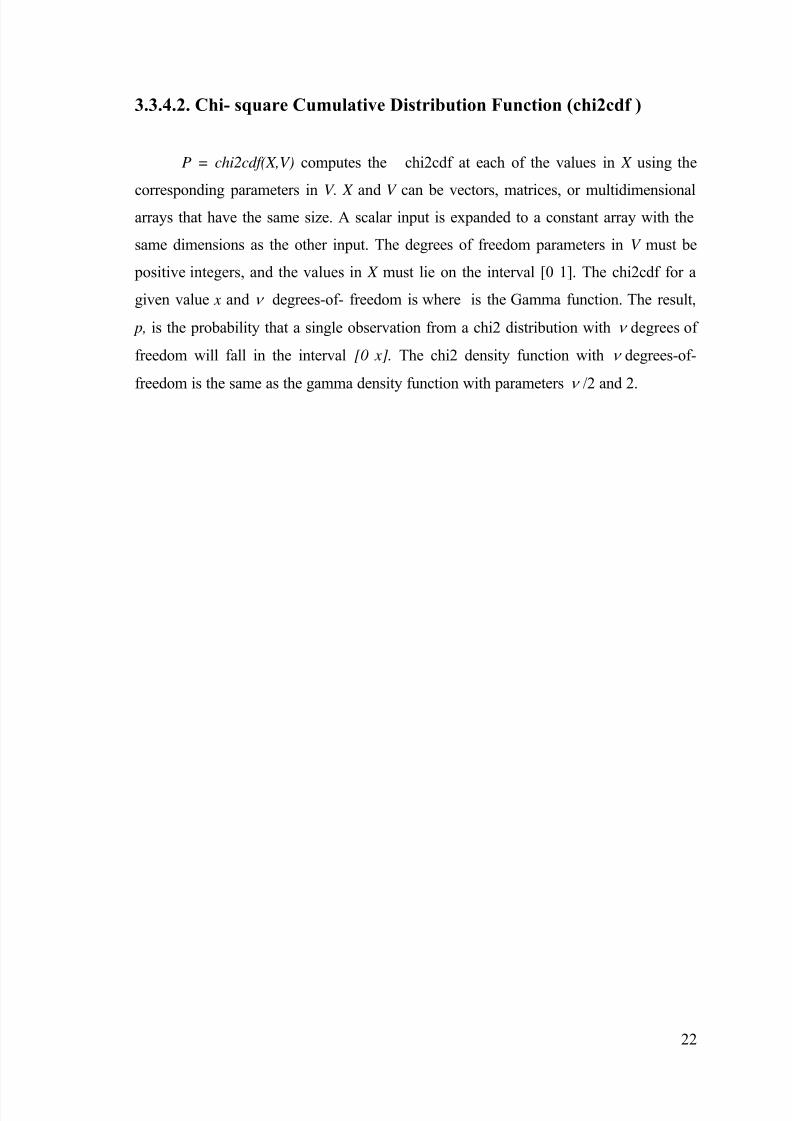
3.3.4.2. Chi-square Cumulative Distribution Function (chi2cdf) ..... 22
CHAPTER 4. RESULTS AND DISCUSSION ........................................................... 23
4.1. Results of OM and NM for Normally Distributed Data................... 23
4.1.1. Application of OM for 0.01 α ..................................................... 24
4.1.2. Application of NM for 0.01 α .................................................... 30
4.2. Results of OM and NM for Non-normally Distributed Data .......... 36
4.2.1. Application of OM for 0.01 α ..................................................... 36
4.2.2. Application of NM for 0.01 α ..................................................... 40
4.3. Results of OM and NM for Industrial Data.................................... 44
4.3.1. Application of OM for 0.01 α ..................................................... 44
4.3.2. Application of NM for 0.01 α ..................................................... 46
CHAPTER 5. CONCLUSIONS AND RECOMMENDATIONS FOR FUTURE
STUDY ................................................................................................. 48
REFERENCES ............................................................................................................... 50
APPENDICES
APPENDIX A................................................................................................................. 52
APPENDIX B ................................................................................................................. 56
APPENDIX C ................................................................................................................. 59
APPENDIX D................................................................................................................. 61

8/22/2019 Development of Univariate Control Chart for Non Normal Data
http://slidepdf.com/reader/full/development-of-univariate-control-chart-for-non-normal-data 8/87
viii
LIST OF FIGURES
Figure Page
Figure 2.1. Structure of a control chart .......................................................................... 5
Figure 3.1. Histogram of the normally distributed data used in this study
(NDNOD) .................................................................................................. 12
Figure 3.2. Histogram of the non- normally distributed data used in this
study (NNDNOD)3.................................................................................... 12
Figure 3.3. Complete industrial data used in this study. ............................................. 14
Figure 3.4. Histogram for normal operation part (950 data points) of
industrial data............................................................................................. 14
Figure 3.5. Check for normality of the ND part (950 data points) of the ID. .............. 15
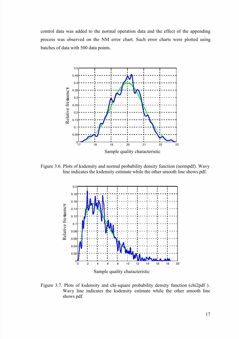
Figure 3.6. Plots of ksdensity and normal probability density function
(normpdf) Wavy line indicates the ksdensity estimate while the
other smooth line shows pdf ...................................................................... 17
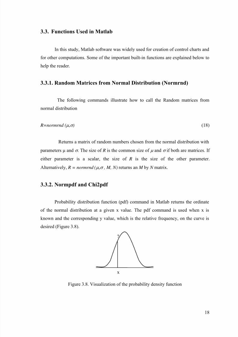
Figure 3.7. Plots of ksdensity and chi-square probability density function
(chi2pdf ).Wavy line indicates the ksdensity estimate while the
other smooth line shows pdf ...................................................................... 17
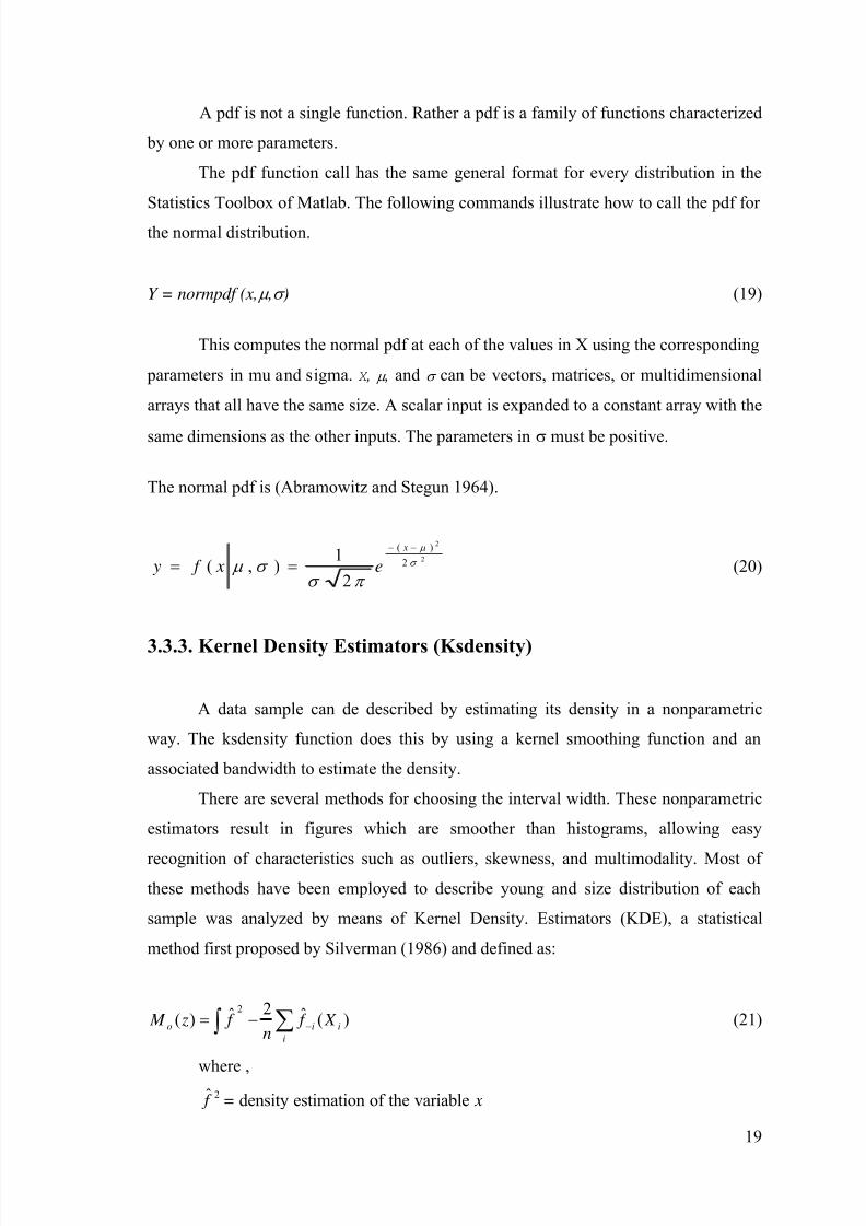
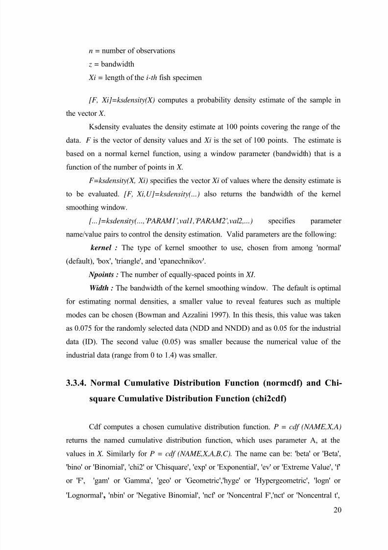
Figure 3.8. Visualization of the probability density function ..................................... 18
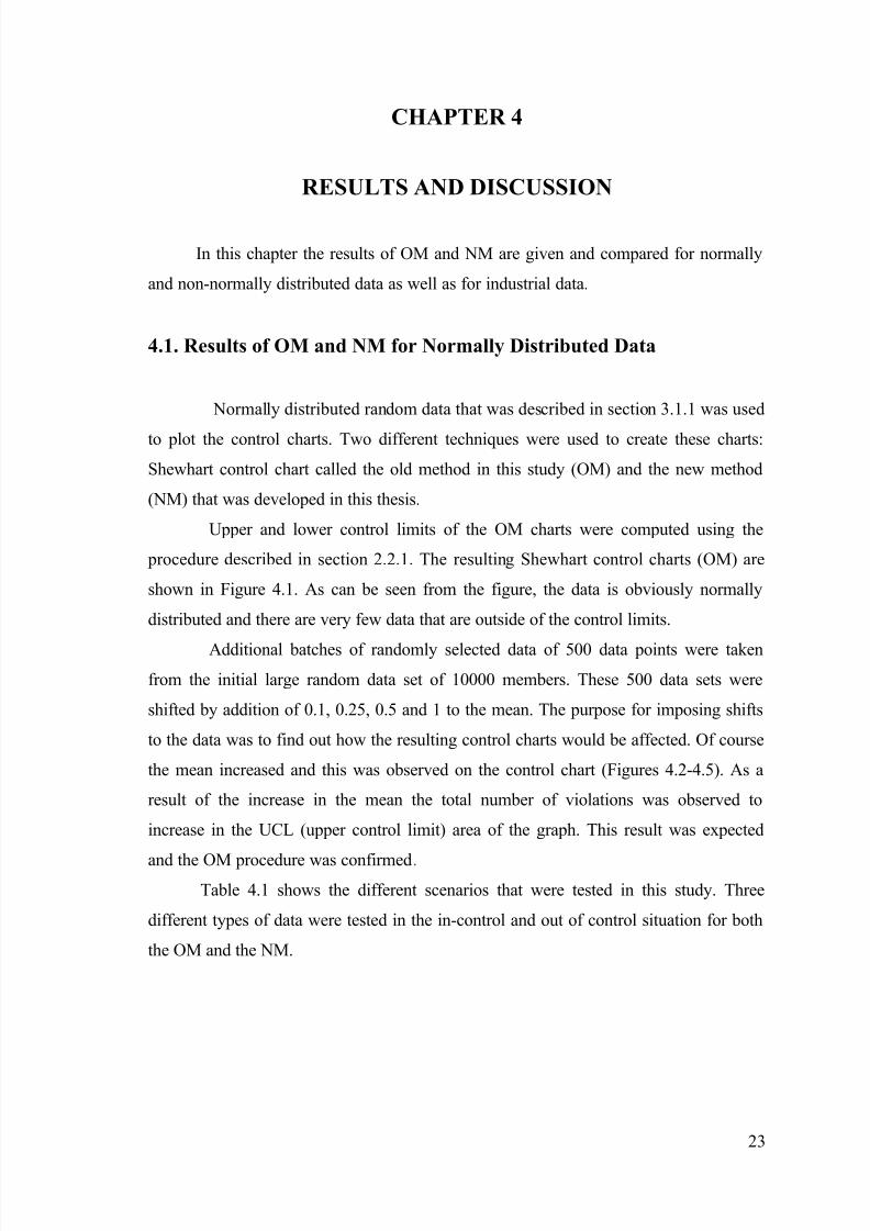
Figure 4.1. Shewhart control chart for normally distributed random data ................... 25
Figure 4.2. Shewhart control chart for normally distributed random data after
its mean is shifted by 0.1 unit. ................................................................... 25
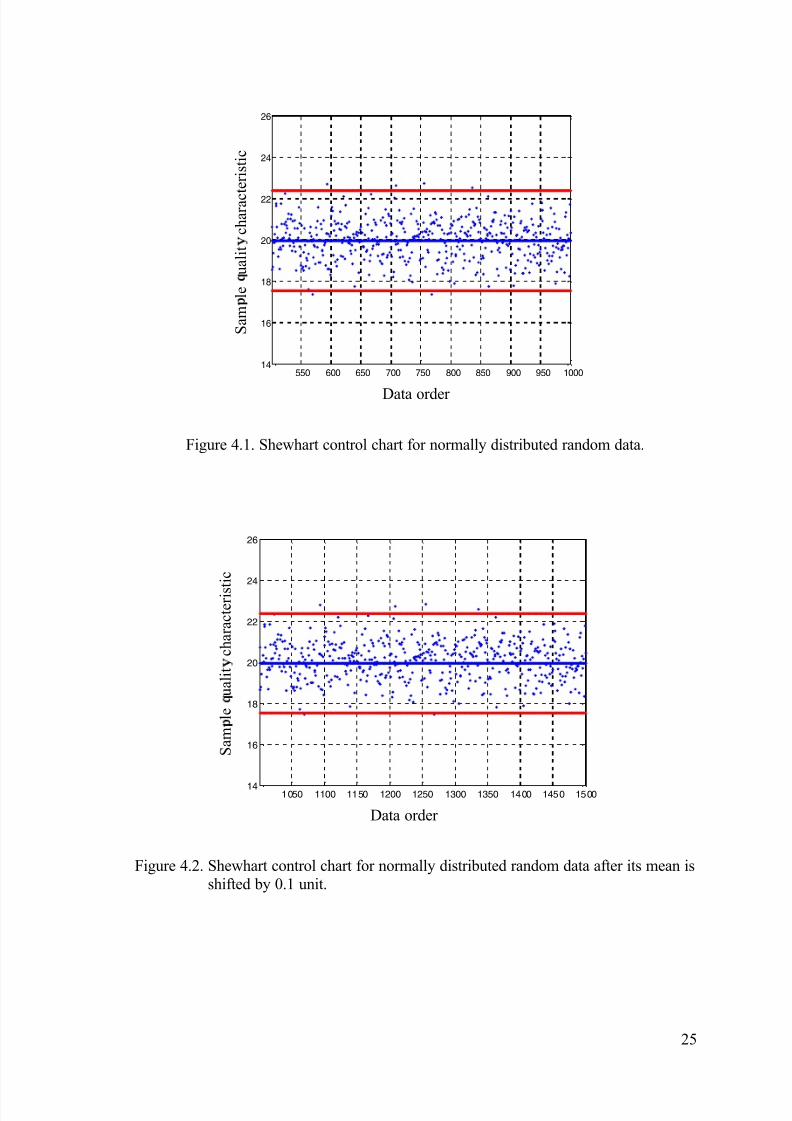
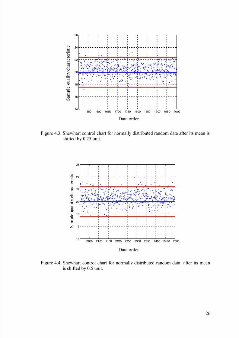
Figure 4.3. Shewhart control chart for normally distributed random data
after its mean is shifted by 0.25 unit.......................................................... 26
Figure 4.4. Shewhart control chart for normally distributed random dataafter its mean is shifted by 0.5 unit............................................................ 26
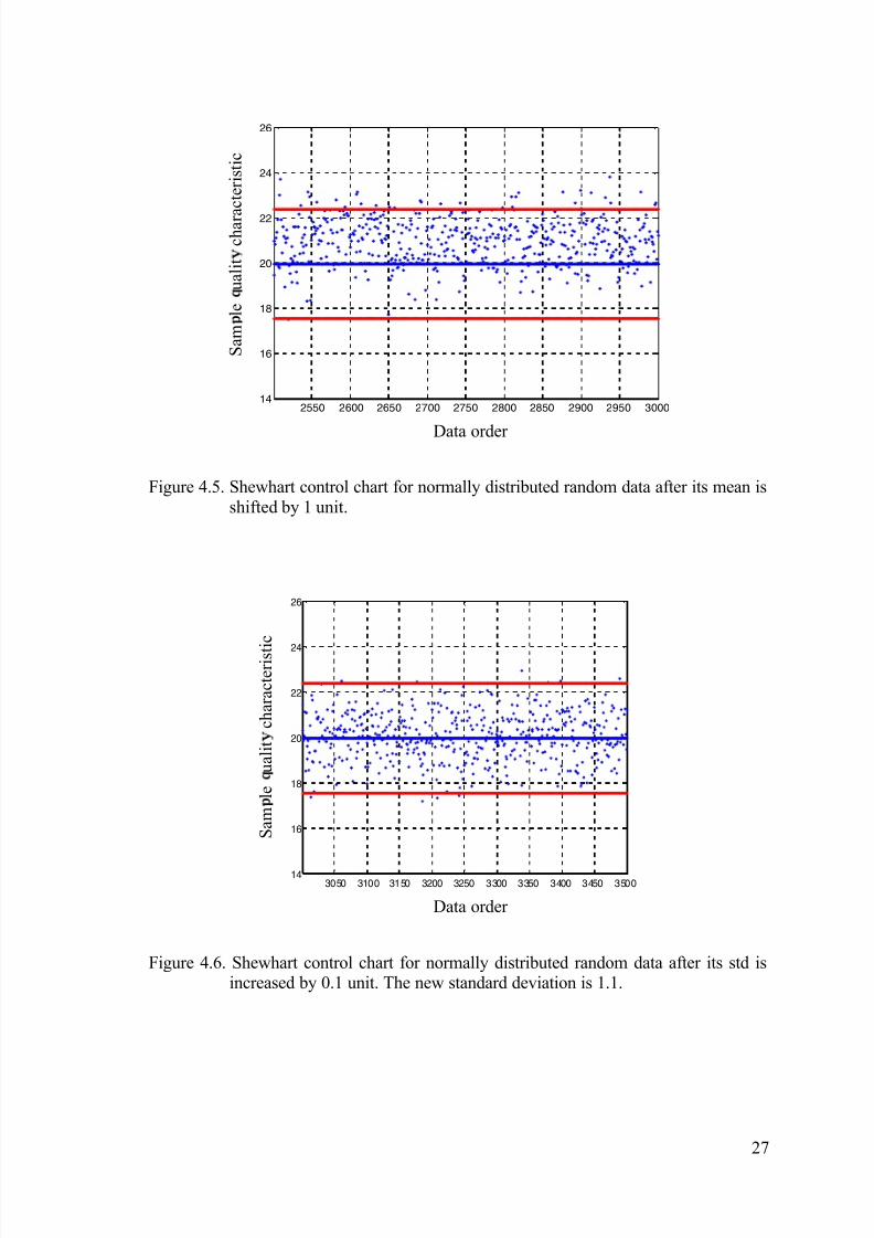
Figure 4.5. Shewhart control chart for normally distributed random data after
its mean is shifted by 1 unit ....................................................................... 27
Figure 4.6. Shewhart control chart for normally distributed random data after
its std is increased by 0.1 unit. The new standard deviation is 1.1............ 27
Figure 4.7. Shewhart control chart for normally distributed random data after
its std is increased by 0.25 unit. The new standard deviation is
1.25 ........................................................................................................... 28

8/22/2019 Development of Univariate Control Chart for Non Normal Data
http://slidepdf.com/reader/full/development-of-univariate-control-chart-for-non-normal-data 9/87
ix
Figure 4.8. Shewhart control chart for normally distributed random data after
its std is increased by 0.5 unit. The new standard deviation is 1.5............ 28
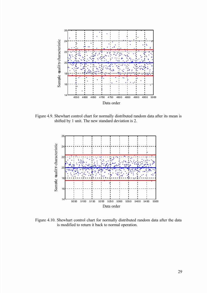
Figure 4.9. Shewhart control chart for normally distributed random data after
its mean is shifted by 1 unit. The new standard deviation is 2 .................. 29
Figure 4.10. Shewhart control chart for normally distributed random data after
the data is modified to return it back to normal operation......................... 29
Figure 4.11. Error control chart for NM for normally distributed random data
when the operation is in-control ............................................................... 30
Figure 4.12. Error chart for normally distributed data after its mean is shifted
by 0.1 unit ................................................................................................. 31
Figure 4.13. Error chart for normally distributed data after its mean is shifted
by 0.25 unit ................................................................................................ 31
Figure 4.14. Error chart for normally distributed data after its mean is shifted
by 0.5 unit .................................................................................................. 32
Figure 4.15. Error chart for normally distributed data after its mean is shifted
by 1 unit ..................................................................................................... 32
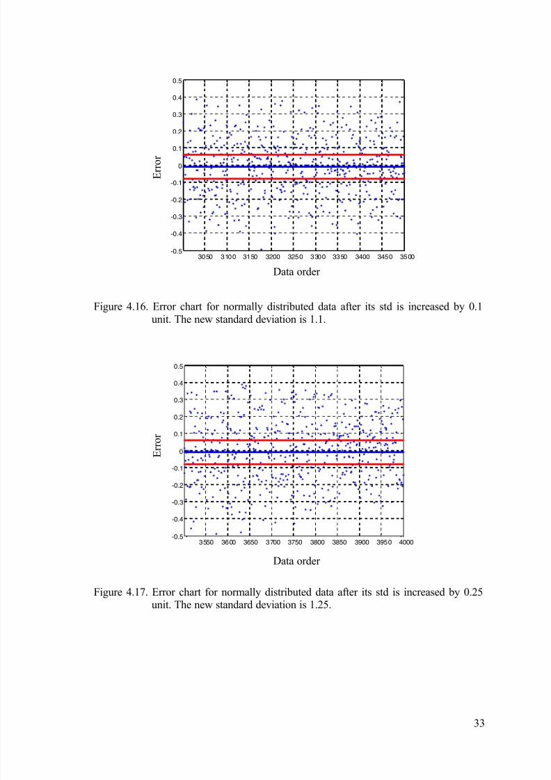
Figure 4.16. Error chart for normally distributed data after its std is increased
by 0.1 unit. The new standard deviation is 1.1 .......................................... 33
Figure 4.17. Error chart for normally distributed data after its std is increased
by 0.25 unit. The new standard deviation is 1.25 ...................................... 33
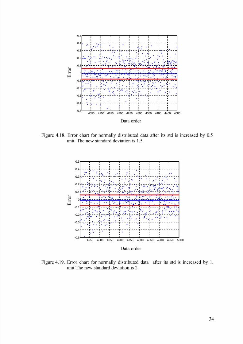
Figure 4.18. Error chart for normally distributed data after its std is increased
by 0.5 unit. The new standard deviation is 1.5 .......................................... 34
Figure 4.19. Error chart for normally distributed data after its std is increased
by 1 unit. The new standard deviation is 2 ................................................ 34
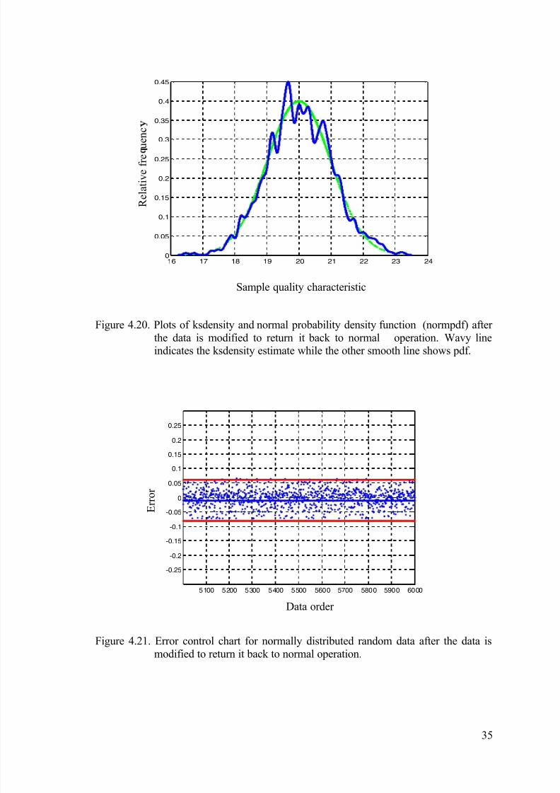
Figure 4.20. Plots of ksdensity and normal probability density function
(normpdf) after the data is modified to return it back to normal
operation Wavy line indicates the ksdensity estimate while the
other smooth line shows pdf ...................................................................... 35
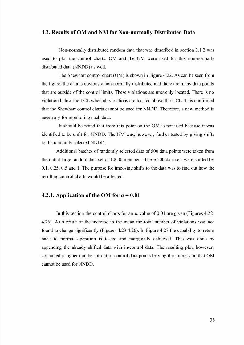
Figure 4.21. Error control chart for normally distributed random data after the
data is modified to return it back to normal operation............................... 35
Figure 4.22. Shewhart control chart for non-normally distributed random data
for in-control situation .............................................................................. 37
Figure 4.23. Shewhart control chart for non-normally distributed random data
after it is shifted by 0.1 unit ....................................................................... 37
8/22/2019 Development of Univariate Control Chart for Non Normal Data
http://slidepdf.com/reader/full/development-of-univariate-control-chart-for-non-normal-data 10/87
x
Figure 4.24. Shewhart control chart for non-normally distributed random data
after it is shifted by 0.25 unit ..................................................................... 38
Figure 4.25. Shewhart control chart for non-normally distributed random data
after it is shifted by 0.5 unit ....................................................................... 38
Figure 4.26. Shewhart control chart for non-normally distributed random data
after it is shifted by 1 unit .......................................................................... 39
Figure 4.27. Shewhart control chart for non-normally distributed random data
after the data is modified to return it back to normal operation ................ 39
Figure 4.28. Error chart for chi-square distributed data (NNDD) for in-
control situation ......................................................................................... 40
Figure 4.29. Error chart for chi-square distributed data (NNDD) after it is
shifted by 0.1 unit .................................................................................... 41
Figure 4.30. Error chart for chi-square distributed data (NNDD) after it is
shifted by 0.25 unit ................................................................................... 41
Figure 4.31. Error chart for chi-square distributed data (NNDD) after it is
shifted by 0.5 unit. ..................................................................................... 42
Figure 4.32. Error chart for chi-square distributed data (NNDD) after it is
shifted by 1 unit ......................................................................................... 42
Figure 4.33. Plots of ksdensity and chi-square probability density function
(chi2pdf ) after the process is returned back to in-control
situation. Wavy line indicates the ksdensity estimate while the
other smooth line shows pdf ...................................................................... 43
Figure 4.34. Error chart for chi-square distributed data (NNDD) after the
process is returned back to in-control situation. ....................................... 43
Figure 4.35. Shewhart control chart for industrial data for normal operation .............. 45
Figure 4.36. Shewhart control chart for industrial data for out-of-control
situation...................................................................................................... 45
Figure 4.37. Plots of ksdensity and normpdf for industrial data for the in-
control situation. Dark continuous line shows ksdensity values
while the dots show pdf values .................................................................. 46
Figure 4.38. Error chart for industrial data for normal operation .................................. 47
Figure 4.39. Error chart for industrial data for out-of control situation ......................... 47

8/22/2019 Development of Univariate Control Chart for Non Normal Data
http://slidepdf.com/reader/full/development-of-univariate-control-chart-for-non-normal-data 11/87
xi
LIST OF TABLES
Table Page
Table 4.1. List of the figures which show the progression of error charts in
this study ....................................................................................................24

8/22/2019 Development of Univariate Control Chart for Non Normal Data
http://slidepdf.com/reader/full/development-of-univariate-control-chart-for-non-normal-data 12/87
xii
GLOSSARY OF ABBREVIATIONS
OM Old Method or the Shewhart Control Chart Method
NM New Method That is Developed in This Thesis
NDD Normally Distributed Data
NNDD Non-normally Distributed Data
NND-ID Non-normally Distributed Industrial Data
ATS Average Time to Signal
ARL Average Run Length
NNDNOD Non-normally Distributed Normal Operation Data
NDNOD Normally Distributed Normal Operation DataEWMA Exponentially Weighted Moving Average
CUSUM Cumulative Sum
CC Control Chart
UCL Upper Control Limit
LCL Lower Control Limit
SPC Statistical Process Control
UWL Upper Warning Limit
LWL Lower Warning Limit
VSI Variable Sampling Interval
ID Industrial Data
CPCT Cumulative Percent Coarser Than
ND Normally Distributed
RF Relative Frequency
KSDENSITY Kernel Smoothing Density Estimation
NORMPDF Normal Probability Density Function
NPDF Normal Probability Density Function
CHI2PDF Chi-square Probability Density Function
NORMRND Random Matrices from Normal Distribution
KDE Kernel Density Estimators
NORMCDF Normal Cumulative Distribution Function
CHI2CDF Non-normal Cumulative Distribution Function
STD Standard Deviation

8/22/2019 Development of Univariate Control Chart for Non Normal Data
http://slidepdf.com/reader/full/development-of-univariate-control-chart-for-non-normal-data 13/87
1
CHAPTER 1
INTRODUCTION
The main work of SQC (Statistical Quality Control) is to control the central
tendency and variability of some processes. A common monitoring tool is to construct
control charts “(Dou and Ping 2002)”. A control chart (CC) is a statistical scheme
(usually allowing graphical implementation) devised for the purpose of checking and
then monitoring the statistical stability of a process.
An efficient CC must continue sampling as long as the process is in-control and
must give an out-of control signal to stop sampling as quickly as possible when the
process becomes out-of-control “(Bakir 2004)”. The major function of control charting
is to detect the occurrence of assignable causes so that the necessary corrective action
may be taken before a large quantity of non-conforming product is manufactured
“(Chou et al. 2001)”. The most widely used method to control the central tendency of a
process is Shewhart-X chart “(Shewhart 1931)” which includes a centerline and two
control limit lines.
There are two other possible alternatives to the Shewhart control charts in the
construction of the central location control charts. One is the CUSUM (Cumulative
Sum) chart and the other is the EWMA (Exponentially Weighted Moving Average)
chart. Both of these concentrate on improving the performance of control charts in
detecting small shifts by using historical data “(Dou and Ping 2002)”.
Various control chart techniques have been developed and widely applied in
process control. Duncan’s cost model “(Duncan 1956)” includes the cost of an out-of-
control condition, the cost of false alarms, the cost of searching for an assignable cause,and the cost of sampling, inspection, evaluation, and plotting. In addition to the
economic design of control charts, another approach to designing a control chart is
called statistical design “(Chou et al. 2001)”.
In real industrial applications, the process populations are frequently not
normally distributed. Burr discussed the effects of non-normality and provided
appropriate control constants for different non-normal populations. All the distributions
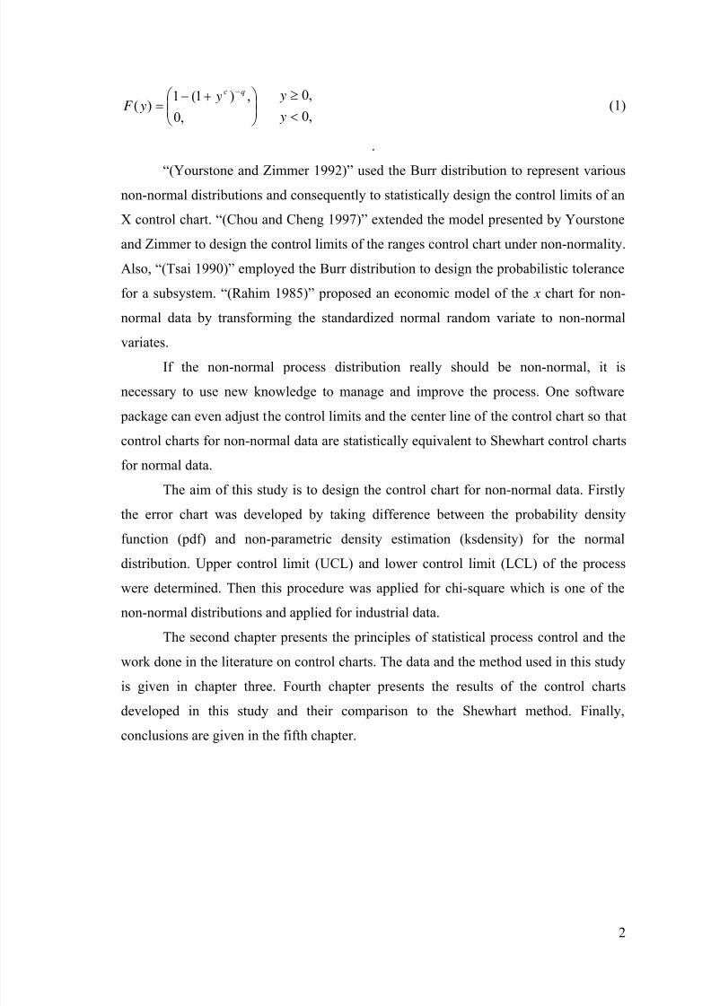
considered belong to the Burr family “(Burr 1967)”, which is of the following form:
8/22/2019 Development of Univariate Control Chart for Non Normal Data
http://slidepdf.com/reader/full/development-of-univariate-control-chart-for-non-normal-data 14/87
2
,0
,0
,0
,)1(1)(
<
≥⎟⎟ ⎠
⎞⎜⎜⎝
⎛ +−=
−
y
y y yF
qc
(1)
.
“(Yourstone and Zimmer 1992)” used the Burr distribution to represent variousnon-normal distributions and consequently to statistically design the control limits of an
X control chart. “(Chou and Cheng 1997)” extended the model presented by Yourstone
and Zimmer to design the control limits of the ranges control chart under non-normality.
Also, “(Tsai 1990)” employed the Burr distribution to design the probabilistic tolerance
for a subsystem. “(Rahim 1985)” proposed an economic model of the x chart for non-
normal data by transforming the standardized normal random variate to non-normal
variates.
If the non-normal process distribution really should be non-normal, it is
necessary to use new knowledge to manage and improve the process. One software
package can even adjust the control limits and the center line of the control chart so that
control charts for non-normal data are statistically equivalent to Shewhart control charts
for normal data.
The aim of this study is to design the control chart for non-normal data. Firstly
the error chart was developed by taking difference between the probability density
function (pdf) and non-parametric density estimation (ksdensity) for the normal
distribution. Upper control limit (UCL) and lower control limit (LCL) of the process
were determined. Then this procedure was applied for chi-square which is one of the
non-normal distributions and applied for industrial data.
The second chapter presents the principles of statistical process control and the
work done in the literature on control charts. The data and the method used in this study
is given in chapter three. Fourth chapter presents the results of the control charts
developed in this study and their comparison to the Shewhart method. Finally,
conclusions are given in the fifth chapter.

8/22/2019 Development of Univariate Control Chart for Non Normal Data
http://slidepdf.com/reader/full/development-of-univariate-control-chart-for-non-normal-data 15/87
3
CHAPTER 2
LITERATURE SURVEY
2.1. Statistical Process Control
It is impossible to inspect or test quality into a product; the product must be built
right the first time. This implies that the manufacturing process must be stable and that
all individuals involved with the process (including operators, engineers, quality
assurance personel, and management) must continuously seek to improve process performance and reduce variability in key parameters. On-line statistical process control
(SPC) is a primary tool for achieving this objective.
If a product is to meet or exceed customer expectations, generally it should be
produced by a process that is stable or repetable. More precisely, the process must be
capable of operating with little variability around the target or nominal dimensions of
the product’s quality characteristics. SPC is a powerful collection of problem-solving
tools useful in achieving process stability and improving capability through the
reduction of variability.
SPC can be applied to any process. Its seven major tools are:
1. Histogram or stem-and-leaf plot
2. Check sheet
3. Pareto chart
4. Cause-and-effect diagram
5. Defect concentration diagram
6. Scatter diagram
7. Control chart
Although these tools, often called “the magnificent seven”, are an important part
of SPC, they comprise only its technical aspects. SPC builds an environment in which
all individuals in an organization seek continous improvement in quality and
productivity. This environment is best developed when management becomes involved
in the process. Once this environment is established, routine application of the
8/22/2019 Development of Univariate Control Chart for Non Normal Data
http://slidepdf.com/reader/full/development-of-univariate-control-chart-for-non-normal-data 16/87
4
magnificent seven becomes part of the usual manner of doing business, and
organization is well on its way to achieving its quality improvement objectives.
Control charts are the simplest type of on-line statistical process control
procedure.
2.2. Control Charts
Control charts are useful for tracking process statistics over time and detecting
the presence of special causes. A special cause results in variation that can be detected
and controlled. Examples of special causes include supplier, shift, or day of the week
differences. Common cause variation, on the other hand, is variation that is inherent in
the process. A process is in control when only common causes - not special causes -
affect the process output.
Variable control charts, described here, plot statistics from measurement data,
such as length or pressure. Attributes control charts plot count data, such as the number
of defects or defective units. For instance, products may be compared against a standard
and classified as either being defective or not. Products may also be classified by their
number of defects. A process statistic, such as a subgroup mean, individual observation, or
weighted statistic, is plotted versus sample number or time. As with variables control
charts, a process statistic, such as the number of defects, is plotted versus sample
number or time for attributes control charts.A “center line” is drawn at the average of
the statistic being plotted for the time being charted. Two other lines - the upper and
lower control limits - are drawn, by default, 3σ above and below the center line (Figure
2.1.)
A process is in control when most of the points fall within the bounds of the
control limits, and the points do not display any nonrandom pattern.

8/22/2019 Development of Univariate Control Chart for Non Normal Data
http://slidepdf.com/reader/full/development-of-univariate-control-chart-for-non-normal-data 17/87
5
Sample number (or time)
Q u a l i t y c h a r a
c t e r i s t i c
Upper Control Limit
Lower Control Limit
Center Line
Figure 2.1. Structure of a control chart
The number of sampling instances before the CC signals is called the run length,
which we denote by L. The efficiency of a CC depends on the distribution of the run
length L. The most common and simplest efficiency criterion is to consider the average
run length (ARL), which is the expected value of the run length distribution. It is
desirable that the ARL of a CC be large if the process is in-control and be small if the
process is out-of-control “(Chou et al. 2004)”. The false alarm rate is the probability that
the CC gives an out-of-control signal when in fact the process is in-control. Most
control charts are distribution-based procedures in the sense that the observations made
on the process output are assumed to follow a specified probability CCs. “(Amin et al.
1995)” found a pronounced difference in the values of the in-control ARL of the
Shewhart X-bar chart under various distributions. Assuming a known standard deviation
and a sample size of n=10, they found the exact values of the in-control ARLs of the
traditional (one-sided) xσ 3 Shewhart X-bar to be: 1068.7 under a uniform distribution,
740.8 under a normal distribution, 441.9 under a double exponential distribution, and11.7 under a Cauchy distribution. This implies that for heavy-tailed underlying
distributions, false alarms will occur much more frequently than expected when the
process is operating in-control. For example, when the process has a Cauchy
distribution, the in-control ARL will only be 11.7, which entails almost 63 times as
many false alarms as the anticipated ARL value of 740.8 associated with the
traditional xσ 3 Shewhart control limits “(Bakir 2004)”.

8/22/2019 Development of Univariate Control Chart for Non Normal Data
http://slidepdf.com/reader/full/development-of-univariate-control-chart-for-non-normal-data 18/87
6
Traditionally, when the issue on designing control chart is discussed, one usually
assumes the measurements in each sampled subgroup (or say population) are normally
distributed; therefore, the sample mean X is also normally distributed “(Chou et al.
2004)”.
2.2.1. Control Charts for Normal Data
In this section control charts for normal data are explained. First Shewhart
Control Charts are discussed followed by some introductory information about the ARL
and ATS.
2.2.1.1. Shewhart Control Chart
Since 1924 when Dr. Shewhart presented the first control chart, various control
chart techniques have been developed and widely applied as a primary tool in statistical
process control. A survey by “(Saniga and Shirland 1977)” indicated that the control
chart for averages (or the X chart) dominates the use of any other control chart
technique if quality is measured on a continuous scale “(Chou 2001)”.
When the X control chart is used to monitor a process, three parameters should
be determined: the sample size, the sampling interval between successive samples, and
the control limits of the chart which are UCL(Upper Control Limit) and LCL (Lower
Control Limit) “(Chou 2000)”:
X K X UCL σ += (2)
X CL = (3)
X K X LCL σ −= (4)
where
m
X X X X m+++
=...21 (5)
8/22/2019 Development of Univariate Control Chart for Non Normal Data
http://slidepdf.com/reader/full/development-of-univariate-control-chart-for-non-normal-data 19/87
7
is the grand average, K is the control constant and X σ is the standard deviation of
sample mean and m is the number of samples taken. There are tables available for
values of K based on the sample sizes and process requirements “(Montgomery 2005)”.
Shewhart also suggested 3-sigma control limits as action limits and sample sizes of four or five, leaving the interval between successive subgroups to be determined by the
practitioner “(Chou 2001)”.
In process control using Shewhart Control Charts, common practice is to
observe for data points that lie outside of the control limits during normal operation.
When such data are collected there are criteria that are developed to determine whether
the process is out of control. These are known as run-rules. Western Electric Handbook
presents a comprehensive discussion of the issue “(Western Electric Handbook 1956)”.
2.2.1.2. Calculation of ARL and ATS
In-control average run length(ARL), out-of-control ARL and average time to
signal were evaluated for α=0.01. These values were computed by equation 6, 7 and 8
“(Montgomery 2005)”.
In-control ARL=α
10 = ARL (6)
Out-of-control ARL= β −
=1
11 ARL (7)
ATS=ARL*h (8)
⎥⎦
⎤
⎢⎣
⎡ +−Φ−
⎥⎦
⎤
⎢⎣
⎡ +−Φ=
n
k LCL
n
k UCL
/
)(
/
)( 00
σ
σ µ
σ
σ µ β (9)
where α is the probability of making type I error, β is the probability of making type II
error, h is time, Φ is the cumulative distribution function and µ o is the mean in the in-
control case.
8/22/2019 Development of Univariate Control Chart for Non Normal Data
http://slidepdf.com/reader/full/development-of-univariate-control-chart-for-non-normal-data 20/87
8
2.2.1.3. Statistically Designed Control Charts
Statistically designed control charts are those in which control limits (which
determine the Type I error probability, α) and power are preselected. These thendetermine the sample size and, if the average time to signal is specified, the sampling
interval “(Woodall,1985)”. “(Saniga 1989)” incorporated the concept of statistical
considerations into the economic design of the control charts and then presented the
`economic statistical design’ of the joint X and R charts for normal data
2.2.2. Control Charts for Non-Normal Data
The normality assumption may not be tenable every time. For example, the
distributions of measurements from chemical processes, semiconductor processes, or
cutting tool wear process are often skewed “(Chang and Bai, 2001)”. If the
measurements are really normally distributed, the statistic X, which is the sample
characteristic of interest, is also normally distributed. If the measurements are
asymmetrically distributed, the statistic X will be approximately normally distributed
only when the sample size n is sufficiently large (based on the central limit theorem)
and when its. Unfortunately, when a control chart is applied to monitor the process, the
sample size n is always not sufficiently large due to the sampling cost. Therefore, if the
measurements are not normally distributed, the traditional way for designing the control
chart may reduce the ability that a control chart detects the assignable causes “(Chou
2001)”.
The non-normal behavior of measurements may imply that the traditional design
approach is improper for the operation of control charts.
2.2.2.1. Burr Distribution
The Burr cumulative distribution function “(Burr, 1942)” is
,0,)1(
11)( ≥
+−= for
y yF
qc(10)

8/22/2019 Development of Univariate Control Chart for Non Normal Data
http://slidepdf.com/reader/full/development-of-univariate-control-chart-for-non-normal-data 21/87
9
where c and q are greater than 1. “(Burr 1967)” applied his distribution to study the
effect of non-normality on the constants of X and R control charts. “(Burr 1942)”
tabulated the expected value, standard deviation, skewness coefficient, and kurtosis
coefficient of the Burr distribution for various combinations of c and q. These tables
allow the users to make a standardized transformation between a Burr variate (say, Y)
and another random variate (X)
Denote UCL, LCL, UWL, and LWL as the upper control limit, lower control
limit, upper warning limit, and lower warning limit, respectively. Expressed
mathematically, we obtain
,/0 nk UCL σ µ += ,/0 nk LCL σ µ −= (11)
,/0 nwUWL σ µ += ,/0 nw LWL σ µ −= (12)
where µ0 is the process mean when the process is in control. In this article, to simplify
the model, we assume that when the process is out of control, the process mean shifts
to δσ += 01 , but the process standard deviation remains unchanged. The Burr
random variate Y can be transformed to the sample statistic X by the standardized
procedure as follows:
n
X
S
M Y
/σ
µ −=
−(13)
That is, the scale and origin of the fitted Y values are changed to those of the X
values, and from Equation above, when the process is in-control, we obtain,
S
n M Y X
/)(0
σ µ −+= (14)
When the process is out-of-control, X is assumed to follow a Burr distribution
with mean δσ +0 and standard deviation n/σ “(Chou 2004)”.

8/22/2019 Development of Univariate Control Chart for Non Normal Data
http://slidepdf.com/reader/full/development-of-univariate-control-chart-for-non-normal-data 22/87
10
2.2.2.2. The Variable Sampling Interval (VSI) X control chart
Assume that the distribution of measurements from a process is non-normally
distributed, and has the mean µ and standard deviationσ . When an X control chart
(with centerline 0 ; the upper control limit )/(10 nk σ µ + and the lower control limit
)/(10 nk σ µ ′− where 1k and 1k ′ are not necessarily equal) is used for monitoring the
process, a sample of size n is taken and calculated its sample mean at each sampling
point to judge whether or not the process remains in-control state. If the sample
meani X plotted on the control X chart goes beyond the control limits, then a signal
will be given to inform the operator to search for the assignable cause. Otherwise, the
process is considered being in-control, and the next sample is continually taken at next
sampling point
In this situation, the control chart operates with fixed sampling interval (say h1)
regardless of i X which is said to be the FSI control chart.
For VSI control charts, if the sample mean falls inside the control limits, the
monitored process is also considered stable as FSI chart. However, with a difference to
the FSI charts, the next sampling interval will be a function of this sample mean. That
is, the next sampling rate depends on the current sample mean.
Assume the VSI X chart uses a unite number of sampling interval lengths, say
h1, h2, … hm; where h1<h2<…<hm; and m≥2. The choice of a sampling interval can be
made by a function h(x) when the value of i X is measured. Burr distribution can be
implemented for the economic design of the VSI chart in monitoring non-normal
process data.

8/22/2019 Development of Univariate Control Chart for Non Normal Data
http://slidepdf.com/reader/full/development-of-univariate-control-chart-for-non-normal-data 23/87
11
CHAPTER 3
THE PROPOSED METHOD AND THE MODEL
The methodology used in this study for the development of the new method
(NM) is briefly presented in this section. First of all different data sets were created or
collected from the industry to test the effectiveness of the OM and the NM. Matlab v.7
software was used for computations. A number of built-in functions were employed in
Matlab environment for computations. These functions are explained in section 3.3 and
a complete list of program codes is given in Appendix D.
3.1. The Data
Different types of data were used in this study. Two random selections of 10000
data points were generated in Matlab, the first being normally distributed while the
second was non-normally distributed (chi-square distribution). In addition, industrial
data about the fineness of Portland cement were collected from a local cement plant
(Çimentaş A.Ş.).
3.1.1. Normally Distributed Random Data
Matlab v.7 commercial software was used to create the randomly selected
normally distributed data set. 10000 randomly selected data were produced with an
average of 20 and a standard deviation of 1 (Appendix A). Batches with as much as
1000 data were taken from this 10000 data stock. The first 1000 data (Figure 3.1) were
named “normally distributed normal operation data (NDNOD)” and were used for
calculation of the control limits.
3.1.2. Non-Normally Distributed Random Data
Matlab v.7 commercial software was again used to create the randomly selected
non-normally distributed data set. 10000 randomly selected data points with a chisquare

8/22/2019 Development of Univariate Control Chart for Non Normal Data
http://slidepdf.com/reader/full/development-of-univariate-control-chart-for-non-normal-data 24/87
12
non-normal distribution were created with 5 degrees of freedom (Appendix B). Batches
with as much as 1000 data were taken from this 10000 data stock. The first 1000 data
(Figure 3.2) were named “non-normally distributed normal operation data (NNDNOD)”
and were used for calculation of the control limits.
17 18 19 20 21 22 230
10
20
30
40
50
60
70
80
90
Figure 3.1. Histogram of the normally distributed data used in this study (NDNOD).
0 2 4 6 8 10 12 14 16 18 200
10
20
30
40
50
60
70
80
90
Figure 3.2. Histogram of the non- normally distributed (chi-square) data used in this
study (NNDNOD)
Sample quality characteristic
R e l a t i v e
f r e u e n c
Sample quality characteristic
R e l a t i v e
f r e u e n c
R e l a t i v e f r e u e n c

8/22/2019 Development of Univariate Control Chart for Non Normal Data
http://slidepdf.com/reader/full/development-of-univariate-control-chart-for-non-normal-data 25/87
13
3.1.3. Industrial Data (ID)
Portland cement manufacture process starts with a rotary furnace step in which a
semi-product of clinker is produced. The semi-product is fast-cooled to preserve thecement phases and milled in tube mills with heavy iron ball media. The tube mill is
actually a tumbling ball mill. The product of the mill is a finely ground powder whose
particle size and surface area are closely monitored as a process control tool. One of the
most important parameters is the CPCT 90 micrometers (Cumulative Percent Coarser
Than) which is the oversized weight percentage above a 90 micrometer sieve. This data
is collected once in every hour. For effective cement hydration reaction this percentage
must be controlled within predetermined limits. The percentage of milled product larger
than (cumulative percent larger than: CPCT) the 90 micrometer sieve was measured and
recorded (DACK 90) in the cement plant as a process control parameter.
There were a total of 1179 data points that were collected from the plant (Figure
3.3 and Appendix C). Average CPCT 90 micrometer value was 0.5614 with a standard
deviation of 0.3262. The data was partitioned into two sets based on the observation that
the process was out-of control after the 951st data point. Therefore the first part with 950
data points was called the ID for normal operation. The remaining 229 data points were
for the out-of-control situation.
Histogram for industrial data is presented in Figure 3.4 for normal operation. In
order to identify the type of the reference distribution with which the industrial data
could be associated, a number of tests were done. As a result of the first visual
inspection the data could be identified non-normal. Therefore, a chisquare type of
distribution was attempted first. For this purpose the normplot function of Matlab was
employed and the resulting graph is shown in Figure 3.5. When the crosses are located
on the diagonal red line the distribution is normal. The more the crosses deviate away
from the diagonal red line, the less becomes the normality. As can be seen in Figure 3.5.
the ID used in this study was not normally distributed.

8/22/2019 Development of Univariate Control Chart for Non Normal Data
http://slidepdf.com/reader/full/development-of-univariate-control-chart-for-non-normal-data 26/87
14
0 200 400 600 800 1000 12000
0.5
1
1.5
2
2.5
3
3.5
4
Figure 3.3. Complete industrial data used in this study.
-0.2 0 0.2 0.4 0.6 0.8 1 1.2 1.40
50
100
150
200
250
Figure 3.4. Histogram for normal operation part (950 data points) of industrial data.
Data order
Sample quality characteristic
S a m
l e
u a l i t c
h a r a c t e r i s t i c
R e l a t i v e f r e u e n c

8/22/2019 Development of Univariate Control Chart for Non Normal Data
http://slidepdf.com/reader/full/development-of-univariate-control-chart-for-non-normal-data 27/87
15
0 0.2 0.4 0.6 0.8 1 1.2
0.001
0.003
0.010.02
0.05
0.10
0.25
0.50
0.75
0.90
0.95
0.980.99
0.997
0.999
Data
P r o b a b i l i t y
Normal Probability Plot
Figure 3.5. Check for normality of the ND part (950 data points) of the ID.
3.2. Proposed Methodology
SPC is usually carried out by plotting the control charts for normal operation
data in order to check for violations that are outside the control limits. In this study, twoseparate control charts were produced from the normal operation data which was
regarded as ideal, in-control situation. The first was the OM which utilized the well
known Shewhart Control Chart approach while the second was developed in this study
and was named the new method (NM).
3.2.1. The Shewhart Method (OM)
The theory of Shewhart control charts is given in section 2.2.1. Normal
operation data (NDNOD) were analyzed to determine its standard deviation, upper and
lower control limits via equations 2, 3, 4 and 5. Using these values the control chart was
created. Different levels of shifts were imposed on the data to observe the control chart
performance when the process gets out of control. In such a case operator intervention is
required. Shifts as much as 0.1, 0.25, 0.5 and 1σ were made to the mean. In addition,
the standard deviation was increased by 1.1, 1.25, 1.5 and 2. Finally, tests were
8/22/2019 Development of Univariate Control Chart for Non Normal Data
http://slidepdf.com/reader/full/development-of-univariate-control-chart-for-non-normal-data 28/87
16
conducted to make sure the process could be returned to normal operation. Same
procedure was repeated for NNDNOD.
3.2.2. The New Method (NM)
Shewhart charts (OM) are well known and effectively used for normally
distributed data as a process control tool. However, they are known to be deficient in the
monitoring of non-normally distributed data. Therefore, a new method is proposed in
this thesis to create a control chart for non-normally distributed data. The method works
by first computing a ksdensity function using the built-in function of Matlab
(ksdensity). Secondly either a normpdf or a chi2pdf function is computed. The
mathematical basis for the two functions is presented in section 3.3. When the data was
normally distributed the error was calculated by taking the difference between ksdensity
and normpdf via equation 16. For non-normally distributed data, however, the
difference between ksdensity and chi2pdf was used for error calculation (Eq. 17). The
control chart developed in the new method contained the error as a process control
measure in contrast to the original data itself that was used in the OM.
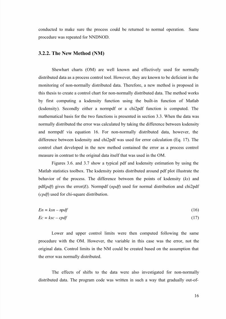
Figures 3.6. and 3.7 show a typical pdf and ksdensity estimation by using the
Matlab statistics toolbox. The ksdensity points distributed around pdf plot illustrate the
behavior of the process. The difference between the points of ksdensity (ks) and
pdf( pdf ) gives the error( E ). Normpdf (npdf ) used for normal distribution and chi2pdf
(cpdf ) used for chi-square distribution.
En = ksn – npdf (16)
Ec = ksc – cpdf (17)
Lower and upper control limits were then computed following the same
procedure with the OM. However, the variable in this case was the error, not the
original data. Control limits in the NM could be created based on the assumption that
the error was normally distributed.
The effects of shifts to the data were also investigated for non-normally
distributed data. The program code was written in such a way that gradually out-of-
8/22/2019 Development of Univariate Control Chart for Non Normal Data
http://slidepdf.com/reader/full/development-of-univariate-control-chart-for-non-normal-data 29/87
17
control data was added to the normal operation data and the effect of the appending
process was observed on the NM error chart. Such error charts were plotted using
batches of data with 500 data points.
17 18 19 20 21 22 230
0.05
0.1
0.15
0.2
0.25
0.3
0.35
0.4
0.45
0.5
Figure 3.6. Plots of ksdensity and normal probability density function (normpdf). Wavy
line indicates the ksdensity estimate while the other smooth line shows pdf.
0 2 4 6 8 10 12 14 16 18 200
0.02
0.04
0.06
0.08
0.1
0.12
0.14
0.16
0.18
0.2
Figure 3.7. Plots of ksdensity and chi-square probability density function (chi2pdf ).
Wavy line indicates the ksdensity estimate while the other smooth line
shows pdf.
Sample quality characteristic
Sample quality characteristic
R e l a t i v e f r e u e n c
R e l a t i v e f r e u e n c
8/22/2019 Development of Univariate Control Chart for Non Normal Data
http://slidepdf.com/reader/full/development-of-univariate-control-chart-for-non-normal-data 30/87
18
3.3. Functions Used in Matlab
In this study, Matlab software was widely used for creation of control charts and
for other computations. Some of the important built-in functions are explained below tohelp the reader.
3.3.1. Random Matrices from Normal Distribution (Normrnd)
The following commands illustrate how to call the Random matrices from
normal distribution
R=normrnd (µ,σ ) (18)
Returns a matrix of random numbers chosen from the normal distribution with
parameters µ and σ . The size of R is the common size of µ and σ if both are matrices. If
either parameter is a scalar, the size of R is the size of the other parameter.
Alternatively, R = normrnd (µ,σ , M, N) returns an M by N matrix.
3.3.2. Normpdf and Chi2pdf
Probability distribution function (pdf) command in Matlab returns the ordinate
of the normal distribution at a given x value. The pdf command is used when x is
known and the corresponding y value, which is the relative frequency, on the curve is
desired (Figure 3.8).
Figure 3.8. Visualization of the probability density function
x
?
8/22/2019 Development of Univariate Control Chart for Non Normal Data
http://slidepdf.com/reader/full/development-of-univariate-control-chart-for-non-normal-data 31/87
19
A pdf is not a single function. Rather a pdf is a family of functions characterized
by one or more parameters.
The pdf function call has the same general format for every distribution in the
Statistics Toolbox of Matlab. The following commands illustrate how to call the pdf for
the normal distribution.
Y = normpdf (x,µ ,σ ) (19)
This computes the normal pdf at each of the values in X using the corresponding
parameters in mu and sigma. X , µ , and σ can be vectors, matrices, or multidimensional
arrays that all have the same size. A scalar input is expanded to a constant array with the
same dimensions as the other inputs. The parameters in σ must be positive.
The normal pdf is (Abramowitz and Stegun 1964).
2
2
2
)(
2
1),( σ
µ
π σ σ µ
−−
== x
e x f y (20)
3.3.3. Kernel Density Estimators (Ksdensity)
A data sample can de described by estimating its density in a nonparametric
way. The ksdensity function does this by using a kernel smoothing function and an
associated bandwidth to estimate the density.
There are several methods for choosing the interval width. These nonparametric
estimators result in figures which are smoother than histograms, allowing easy
recognition of characteristics such as outliers, skewness, and multimodality. Most of
these methods have been employed to describe young and size distribution of each
sample was analyzed by means of Kernel Density. Estimators (KDE), a statistical
method first proposed by Silverman (1986) and defined as:
∑∫ −−=i
iio X f n
f z M )(ˆ2ˆ)(2
(21)
where ,2ˆ f = density estimation of the variable x
8/22/2019 Development of Univariate Control Chart for Non Normal Data
http://slidepdf.com/reader/full/development-of-univariate-control-chart-for-non-normal-data 32/87
20
n = number of observations
z = bandwidth
Xi = length of the i-th fish specimen
[F, Xi]=ksdensity(X) computes a probability density estimate of the sample in
the vector X .
Ksdensity evaluates the density estimate at 100 points covering the range of the
data. F is the vector of density values and Xi is the set of 100 points. The estimate is
based on a normal kernel function, using a window parameter (bandwidth) that is a
function of the number of points in X.
F=ksdensity(X, Xi) specifies the vector Xi of values where the density estimate is
to be evaluated. [F, Xi,U]=ksdensity(...) also returns the bandwidth of the kernel
smoothing window.
[...]=ksdensity(...,'PARAM1',val1,'PARAM2',val2,...) specifies parameter
name/value pairs to control the density estimation. Valid parameters are the following:
kernel : The type of kernel smoother to use, chosen from among 'normal'
(default), 'box', 'triangle', and 'epanechnikov'.
Npoints : The number of equally-spaced points in XI .
Width : The bandwidth of the kernel smoothing window. The default is optimal
for estimating normal densities, a smaller value to reveal features such as multiple
modes can be chosen (Bowman and Azzalini 1997). In this thesis, this value was taken
as 0.075 for the randomly selected data (NDD and NNDD) and as 0.05 for the industrial
data (ID). The second value (0.05) was smaller because the numerical value of the
industrial data (range from 0 to 1.4) was smaller.
3.3.4. Normal Cumulative Distribution Function (normcdf) and Chi-square Cumulative Distribution Function (chi2cdf)
Cdf computes a chosen cumulative distribution function. P = cdf (NAME,X,A)
returns the named cumulative distribution function, which uses parameter A, at the
values in X. Similarly for P = cdf (NAME,X,A,B,C). The name can be: 'beta' or 'Beta',
'bino' or 'Binomial', 'chi2' or 'Chisquare', 'exp' or 'Exponential', 'ev' or 'Extreme Value', 'f'
or 'F', 'gam' or 'Gamma', 'geo' or 'Geometric','hyge' or 'Hypergeometric', 'logn' or
'Lognormal', 'nbin' or 'Negative Binomial', 'ncf' or 'Noncentral F','nct' or 'Noncentral t',

8/22/2019 Development of Univariate Control Chart for Non Normal Data
http://slidepdf.com/reader/full/development-of-univariate-control-chart-for-non-normal-data 33/87
21
'ncx2' or 'Noncentral Chi-square', 'norm' or 'Normal', 'poiss' or 'Poisson', 'rayl' or
'Rayleigh', 't' or 'T', 'unif' or 'Uniform', 'unid' or 'Discrete Uniform', 'wbl' or 'Weibull'.
CDF calls many specialized routines that do the calculations. P =
cdf('name',X,A1,A2,A3) returns a matrix of probabilities, where name is a string
containing the name of the distribution, X is a matrix of values, and A, A2, and A3 are
matrices of distribution parameters. Depending on the distribution, some of these
parameters may not be necessary. Vector or matrix inputs for X, A1, A2, and A3 must
have the same size, which is also the size of P. A scalar input for X, A1, A2, or A3 is
expanded to a constant matrix with the same dimensions as the other inputs. cdf is a
utility routine allowing you to access all the cdfs in the Statistics Toolbox by using the
name of the distribution as a parameter.
3.3.4.1. Normal Cumulative Distribution Function (Normcdf)
P = normcdf(X, µ,σ)
[P, PLO, PUP] = normcdf(X, µ , σ , PCOV, alpha)
normcdf(X, µ ,σ ) computes the normal cdf at each of the values in X using the
corresponding parameters in µ and σ . X, µ , and σ can be vectors, matrices, or
multidimensional arrays that all have the same size. A scalar input is expanded to a
constant array with the same dimensions as the other inputs. The parameters in σ must
be positive. [P, PLO, PUP] = normcdf(X,µ , σ , PCOV,α ) produces confidence bounds
for P when the input parameters µ and σ are estimates. PCOV is the covariance matrix
of the estimated parameters. α specifies 100(1 -α )% confidence bounds. The default
value of α is 0.05. PLO and PUP are arrays of the same size as P containing the lower
and upper confidence bounds. The function normdf computes confidence bounds for Pusing a normal approximation to the distribution of the estimate and then transforming
those bounds to the scale of the output P. The computed bounds give approximately the
desired confidence level when you estimateµ, σ , and PCOV from large samples, but in
smaller samples other methods of computing the confidence bounds might be more
accurate. The normal cdf is he result, p, is the probability that a single observation from
a normal distribution with parameters µ and will fall in the interval (- x]. The standard
normal distribution has µ= 0 and σ = 1
8/22/2019 Development of Univariate Control Chart for Non Normal Data
http://slidepdf.com/reader/full/development-of-univariate-control-chart-for-non-normal-data 34/87
22
3.3.4.2. Chi- square Cumulative Distribution Function (chi2cdf )
P = chi2cdf(X,V) computes the chi2cdf at each of the values in X using the
corresponding parameters in V. X and V can be vectors, matrices, or multidimensionalarrays that have the same size. A scalar input is expanded to a constant array with the
same dimensions as the other input. The degrees of freedom parameters in V must be
positive integers, and the values in X must lie on the interval [0 1]. The chi2cdf for a
given value x and ν degrees-of- freedom is where is the Gamma function. The result,
p, is the probability that a single observation from a chi2 distribution with ν degrees of
freedom will fall in the interval [0 x]. The chi2 density function with ν degrees-of-
freedom is the same as the gamma density function with parameters ν /2 and 2.
8/22/2019 Development of Univariate Control Chart for Non Normal Data
http://slidepdf.com/reader/full/development-of-univariate-control-chart-for-non-normal-data 35/87
23
CHAPTER 4
RESULTS AND DISCUSSION
In this chapter the results of OM and NM are given and compared for normally
and non-normally distributed data as well as for industrial data.
4.1. Results of OM and NM for Normally Distributed Data
Normally distributed random data that was described in section 3.1.1 was used
to plot the control charts. Two different techniques were used to create these charts:
Shewhart control chart called the old method in this study (OM) and the new method
(NM) that was developed in this thesis.
Upper and lower control limits of the OM charts were computed using the
procedure described in section 2.2.1. The resulting Shewhart control charts (OM) are
shown in Figure 4.1. As can be seen from the figure, the data is obviously normally
distributed and there are very few data that are outside of the control limits.
Additional batches of randomly selected data of 500 data points were taken
from the initial large random data set of 10000 members. These 500 data sets were
shifted by addition of 0.1, 0.25, 0.5 and 1 to the mean. The purpose for imposing shifts
to the data was to find out how the resulting control charts would be affected. Of course
the mean increased and this was observed on the control chart (Figures 4.2-4.5). As a
result of the increase in the mean the total number of violations was observed to
increase in the UCL (upper control limit) area of the graph. This result was expected
and the OM procedure was confirmed.
Table 4.1 shows the different scenarios that were tested in this study. Three
different types of data were tested in the in-control and out of control situation for both
the OM and the NM.

8/22/2019 Development of Univariate Control Chart for Non Normal Data
http://slidepdf.com/reader/full/development-of-univariate-control-chart-for-non-normal-data 36/87
24
Table 4.1. List of the figures which show the progression of error charts in this study.
Type of Data
NDD NNDD ID
OM Figure 4.1 Figure 4.22 Figure 4.35In-Control
NM Figure 4.11 Figure 4.28 Figure 4.38
OM Figures 4.2-4.9 Figures 4.23-4.26 Figure 4.36Out-of-control
NM Figures 4.12-4.19 Figures 4.29-4.32 Figure 4.39
OM Figure 4.10 Figure 4.27Back to in-
control NM Figures 4.20-4.21 Figures 4.33-4.34
4.1.1. Application of OM for α = 0.01
In this section the control charts for an α value of 0.01 are given (Figures 4.1-
4.9). When the α value increases the L coefficient in UCL or LCL calculation is
decreased and hence the control limits are narrower. The progression of the increase in
the number of violations (out-of-the control limits) with an increase in the amount of
shift of the mean (Figures 4.2-4.5) and the standard deviation (Figure 4.6-4.9) can beclearly observed. In Figure 4.10 the capability to return back to normal operation is
tested and demonstrated. This was achieved by appending the already shifted data with
in-control data.
The lower and upper control limits are calculated for two different α values.
This was done to check how much a narrower control interval could lead to an increase
in the number of violations.
8/22/2019 Development of Univariate Control Chart for Non Normal Data
http://slidepdf.com/reader/full/development-of-univariate-control-chart-for-non-normal-data 37/87
25
550 600 650 700 750 800 850 900 950 100014
16
18
20
22
24
26
Figure 4.1. Shewhart control chart for normally distributed random data.
1050 1100 1150 1200 1250 1300 1350 1400 1450 150014
16
18
20
22
24
26
Figure 4.2. Shewhart control chart for normally distributed random data after its mean is
shifted by 0.1 unit.
Data order
Data order
S a m
l e
u a l i t c
h a r a c t e r i s t i c
S a m
l e
u a l i t c
h a r a c t e r i s t i c
8/22/2019 Development of Univariate Control Chart for Non Normal Data
http://slidepdf.com/reader/full/development-of-univariate-control-chart-for-non-normal-data 38/87
26
1550 1600 1650 1700 1750 1800 1850 1900 1950 200014
16
18
20
22
24
26
Figure 4.3. Shewhart control chart for normally distributed random data after its mean is
shifted by 0.25 unit.
2050 2100 2150 2200 2250 2300 2350 2400 2450 250014
16
18
20
22
24
26
Figure 4.4. Shewhart control chart for normally distributed random data after its meanis shifted by 0.5 unit.
Data order
Data order
S a m
l e
u a l i t c
h a r a c t e r i s t i c
S a m
l e
u a l i t c
h a r a c t e r i s t i c
8/22/2019 Development of Univariate Control Chart for Non Normal Data
http://slidepdf.com/reader/full/development-of-univariate-control-chart-for-non-normal-data 39/87
27
2550 2600 2650 2700 2750 2800 2850 2900 2950 300014
16
18
20
22
24
26
Figure 4.5. Shewhart control chart for normally distributed random data after its mean is
shifted by 1 unit.
30 50 310 0 31 50 3200 3250 3 300 3 350 3 400 3 450 3 50 014
16
18
20
22
24
26
Figure 4.6. Shewhart control chart for normally distributed random data after its std isincreased by 0.1 unit. The new standard deviation is 1.1.
Data order
Data order
S a m
l e
u a l i t c
h a r a c t e r i s t i c
S a m
l e
u a l i t c
h a r a c t e r i s t i c

8/22/2019 Development of Univariate Control Chart for Non Normal Data
http://slidepdf.com/reader/full/development-of-univariate-control-chart-for-non-normal-data 40/87
28
3550 3600 3650 3700 3750 3800 3850 3900 3950 400014
16
18
20
22
24
26
Figure 4.7. Shewhart control chart for normally distributed random data after its std isincreased by 0.25 unit. The new standard deviation is 1.25.
4050 4100 4150 4200 4250 4300 4350 4400 4450 450014
16
18
20
22
24
26
Figure 4.8. Shewhart control chart for normally distributed random data after its std is
increased by 0.5 unit. The new standard deviation is 1.5.
Data order
Data order
S a m
l e
u a l i t c
h a r a c
t e r i s t i c
S a m
l e
u a l i t c
h a r a c t e r i s t i c
8/22/2019 Development of Univariate Control Chart for Non Normal Data
http://slidepdf.com/reader/full/development-of-univariate-control-chart-for-non-normal-data 41/87
29
4550 4600 4650 4700 4750 4800 4850 4900 4950 500014
16
18
20
22
24
26
Figure 4.9. Shewhart control chart for normally distributed random data after its mean is
shifted by 1 unit. The new standard deviation is 2.
5050 5100 5150 5200 5250 5300 5350 5400 5450 550014
16
18
20
22
24
26
Figure 4.10. Shewhart control chart for normally distributed random data after the datais modified to return it back to normal operation.
Data order
Data order
S a m
l e
u a l i t c
h a r a c t e r i s t i c
S a m
l e
u a l i t c
h a r a c t e r i s t i c

8/22/2019 Development of Univariate Control Chart for Non Normal Data
http://slidepdf.com/reader/full/development-of-univariate-control-chart-for-non-normal-data 42/87
30
4.1.2. Application of NM for α = 0.01
In this section the results of the NM are given on control charts that were
developed with control limits calculated for an α value of 0.01. In Figure 4.11 the error chart for normally distributed data (NDD) is presented for the in-control situation upon
application of the new method (NM). The same data (NDD) was purposefully shifted to
observe its response on the error charts (Figures 4.12-4.19). In Figures 4.20 and 4.21 the
capability to return back to normal operation is tested and demonstrated. This was
achieved by appending the already shifted data with in-control data.
100 200 300 400 500 600 700 800 900 1000-0.2
-0.15
-0.1
-0.05
0
0.05
0.1
0.15
0.2
Figure 4.11. Error control chart for NM for normally distributed random data when theoperation is in-control.
Data order
E r r o r

8/22/2019 Development of Univariate Control Chart for Non Normal Data
http://slidepdf.com/reader/full/development-of-univariate-control-chart-for-non-normal-data 43/87
31
1050 1100 1150 1200 1250 1300 1350 1400 1450 1500-0.5
-0.4
-0.3
-0.2
-0.1
0
0.1
0.2
0.3
0.4
0.5
Figure 4.12. Error chart for normally distributed data after its mean is shifted by 0.1
unit.
1550 1600 1650 1700 1750 1800 1850 1900 1950 2000-0.5
-0.4
-0.3
-0.2
-0.1
0
0.1
0.2
0.3
0.4
0.5
Figure 4.13. Error chart for normally distributed data after its mean is shifted by 0.25
unit.
Data order
Data order
E r r o r
E r r o r

8/22/2019 Development of Univariate Control Chart for Non Normal Data
http://slidepdf.com/reader/full/development-of-univariate-control-chart-for-non-normal-data 44/87
32
2050 2100 2150 2200 2250 2300 2350 2400 2450 2500-0.5
-0.4
-0.3
-0.2
-0.1
0
0.1
0.2
0.3
0.4
0.5
Figure 4.14. Error chart for normally distributed data after its mean is shifted by 0.5
unit.
2550 2600 2650 2700 2750 2800 2850 2900 2950 3000-0.5
-0.4
-0.3
-0.2
-0.1
0
0.1
0.2
0.3
0.4
0.5
Figure 4.15. Error chart for normally distributed data after its mean is shifted by 1 unit.
Data order
Data order
E r r o r
E r r o r
8/22/2019 Development of Univariate Control Chart for Non Normal Data
http://slidepdf.com/reader/full/development-of-univariate-control-chart-for-non-normal-data 45/87
33
3050 3100 3150 3200 3250 3300 3350 3400 3450 3500-0.5
-0.4
-0.3
-0.2
-0.1
0
0.1
0.2
0.3
0.4
0.5
Figure 4.16. Error chart for normally distributed data after its std is increased by 0.1
unit. The new standard deviation is 1.1.
3550 3600 3650 3700 3750 3800 3850 3900 3950 4000-0.5
-0.4
-0.3
-0.2
-0.1
0
0.1
0.2
0.3
0.4
0.5
Figure 4.17. Error chart for normally distributed data after its std is increased by 0.25unit. The new standard deviation is 1.25.
Data order
Data order
E r r o r
E r r o r
8/22/2019 Development of Univariate Control Chart for Non Normal Data
http://slidepdf.com/reader/full/development-of-univariate-control-chart-for-non-normal-data 46/87
34
4050 4100 4150 4200 4250 4300 4350 4400 4450 4500-0.5
-0.4
-0.3
-0.2
-0.1
0
0.1
0.2
0.3
0.4
0.5
Figure 4.18. Error chart for normally distributed data after its std is increased by 0.5
unit. The new standard deviation is 1.5.
4550 4600 4650 4700 4750 4800 4850 4900 4950 5000
-0.5
-0.4
-0.3
-0.2
-0.1
0
0.1
0.2
0.3
0.4
0.5
Figure 4.19. Error chart for normally distributed data after its std is increased by 1.unit.The new standard deviation is 2.
Data order
Data order
E r r o r
E r r o r
8/22/2019 Development of Univariate Control Chart for Non Normal Data
http://slidepdf.com/reader/full/development-of-univariate-control-chart-for-non-normal-data 47/87
35
16 17 18 19 20 21 22 23 240
0.05
0.1
0.15
0.2
0.25
0.3
0.35
0.4
0.45
Figure 4.20. Plots of ksdensity and normal probability density function (normpdf) after
the data is modified to return it back to normal operation. Wavy lineindicates the ksdensity estimate while the other smooth line shows pdf.
5100 5200 5300 5400 5500 5600 5700 5800 5900 6000
-0.25
-0.2
-0.15
-0.1
-0.05
0
0.05
0.1
0.15
0.2
0.25
Figure 4.21. Error control chart for normally distributed random data after the data is
modified to return it back to normal operation.
Sample quality characteristic
Data order
R e l a t i v e f r e u e n c
E r r o r
8/22/2019 Development of Univariate Control Chart for Non Normal Data
http://slidepdf.com/reader/full/development-of-univariate-control-chart-for-non-normal-data 48/87
36
4.2. Results of OM and NM for Non-normally Distributed Data
Non-normally distributed random data that was described in section 3.1.2 was
used to plot the control charts. OM and the NM were used for this non-normallydistributed data (NNDD) as well.
The Shewhart control chart (OM) is shown in Figure 4.22. As can be seen from
the figure, the data is obviously non-normally distributed and there are many data points
that are outside of the control limits. These violations are unevenly located. There is no
violation below the LCL when all violations are located above the UCL. This confirmed
that the Shewhart control charts cannot be used for NNDD. Therefore, a new method is
necessary for monitoring such data.
It should be noted that from this point on the OM is not used because it was
identified to be unfit for NNDD. The NM was, however, further tested by giving shifts
to the randomly selected NNDD.
Additional batches of randomly selected data of 500 data points were taken from
the initial large random data set of 10000 members. These 500 data sets were shifted by
0.1, 0.25, 0.5 and 1. The purpose for imposing shifts to the data was to find out how the
resulting control charts would be affected.
4.2.1. Application of the OM for α = 0.01
In this section the control charts for an α value of 0.01 are given (Figures 4.22-
4.26). As a result of the increase in the mean the total number of violations was not
found to change significantly (Figures 4.23-4.26). In Figure 4.27 the capability to return
back to normal operation is tested and marginally achieved. This was done by
appending the already shifted data with in-control data. The resulting plot, however,
contained a higher number of out-of-control data points leaving the impression that OM
cannot be used for NNDD.
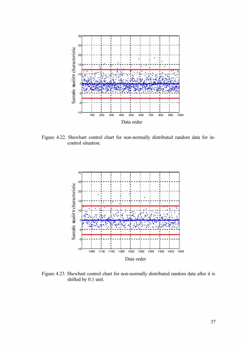
8/22/2019 Development of Univariate Control Chart for Non Normal Data
http://slidepdf.com/reader/full/development-of-univariate-control-chart-for-non-normal-data 49/87
37
100 200 300 400 500 600 700 800 900 1000-10
-5
0
5
10
15
20
25
30
Figure 4.22. Shewhart control chart for non-normally distributed random data for in-
control situation.
1050 1100 1150 1200 1250 1300 1350 1400 1450 1500-10
-5
0
5
10
15
20
25
30
Figure 4.23. Shewhart control chart for non-normally distributed random data after it is
shifted by 0.1 unit.
Data order
Data order
S a m
l e
u a l i t c
h a r a c t e r i s t i c
S a m
l e
u a l i t c
h a r a c t e r i s t i c
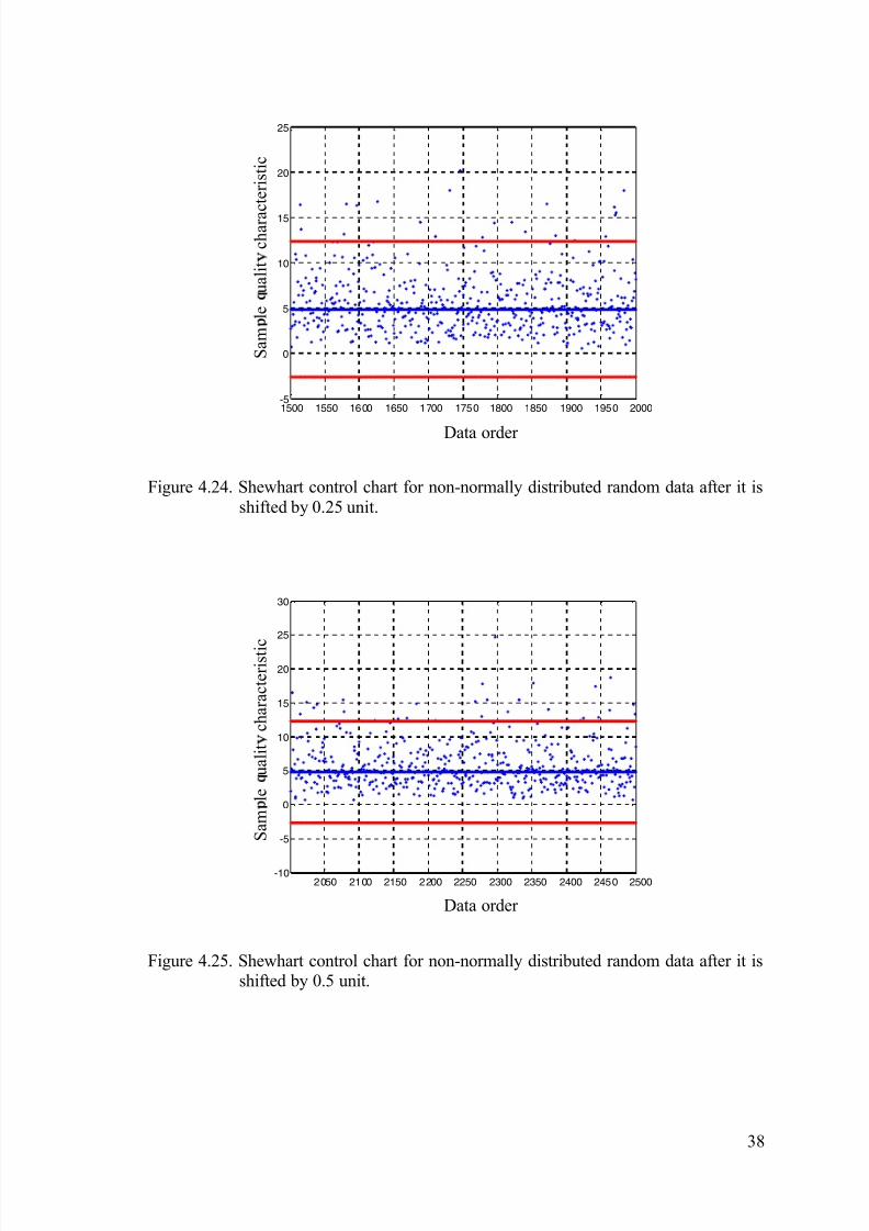
8/22/2019 Development of Univariate Control Chart for Non Normal Data
http://slidepdf.com/reader/full/development-of-univariate-control-chart-for-non-normal-data 50/87
38
1500 1550 1600 1650 1700 1750 1800 1850 1900 1950 2000-5
0
5
10
15
20
25
Figure 4.24. Shewhart control chart for non-normally distributed random data after it is
shifted by 0.25 unit.
2050 2100 2150 2200 2250 2300 2350 2400 2450 2500-10
-5
0
5
10
15
20
25
30
Figure 4.25. Shewhart control chart for non-normally distributed random data after it isshifted by 0.5 unit.
Data order
Data order
S a m
l e
u a l i t c
h a r a
c t e r i s t i c
S a m
l e
u a l i t c
h a r a c t e r i s t i c

8/22/2019 Development of Univariate Control Chart for Non Normal Data
http://slidepdf.com/reader/full/development-of-univariate-control-chart-for-non-normal-data 51/87
39
2550 2600 2650 2700 2750 2800 2850 2900 2950 3000-10
-5
0
5
10
15
20
25
30
Figure 4.26. Shewhart control chart for non-normally distributed random data after it is
shifted by 1 unit.
3000 3100 3200 3300 3400 3500 3600 3700 3800 3900 4000-5
0
5
10
15
20
25
Figure 4.27. Shewhart control chart for non-normally distributed random data after the
data is modified to return it back to normal operation.
Data order
Data order
S a m
l e
u a l i t c
h a r a c t e r i s t i c
S a m
l e
u a l i t c
h a r a c t e r i s t i c
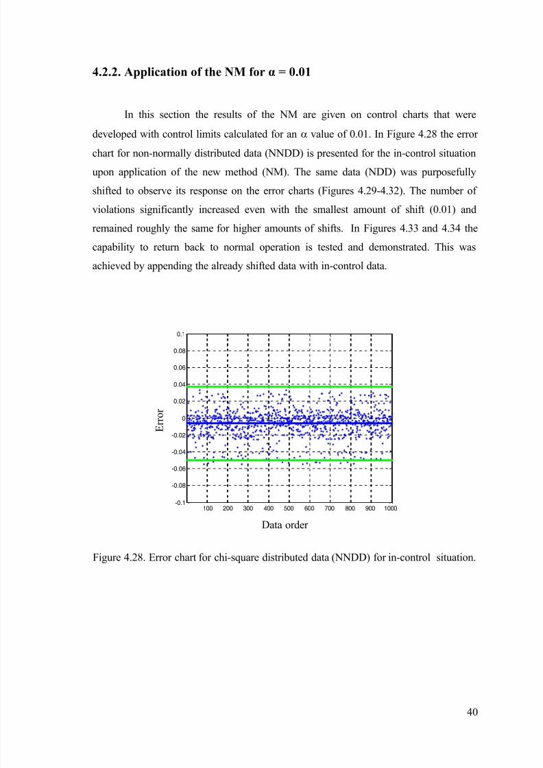
8/22/2019 Development of Univariate Control Chart for Non Normal Data
http://slidepdf.com/reader/full/development-of-univariate-control-chart-for-non-normal-data 52/87
40
4.2.2. Application of the NM for α = 0.01
In this section the results of the NM are given on control charts that were
developed with control limits calculated for an α value of 0.01. In Figure 4.28 the error
chart for non-normally distributed data (NNDD) is presented for the in-control situation
upon application of the new method (NM). The same data (NDD) was purposefully
shifted to observe its response on the error charts (Figures 4.29-4.32). The number of
violations significantly increased even with the smallest amount of shift (0.01) and
remained roughly the same for higher amounts of shifts. In Figures 4.33 and 4.34 the
capability to return back to normal operation is tested and demonstrated. This was
achieved by appending the already shifted data with in-control data.
100 200 300 400 500 600 700 800 900 1000-0.1
-0.08
-0.06
-0.04
-0.02
0
0.02
0.04
0.06
0.08
0.1
Figure 4.28. Error chart for chi-square distributed data (NNDD) for in-control situation.
Data order
E r r o r

8/22/2019 Development of Univariate Control Chart for Non Normal Data
http://slidepdf.com/reader/full/development-of-univariate-control-chart-for-non-normal-data 53/87
41
1050 110 0 1150 1200 12 50 1300 1350 1400 1450 15 00
-0.25
-0.2
-0.15
-0.1
-0.05
0
0.05
0.1
0.15
0.2
0.25
Figure 4.29. Error chart for chi-square distributed data (NNDD) after it is shifted by 0.1
unit.
15 50 1600 1650 1700 1750 1800 18 50 1900 1950 2000
-0.25
-0.2
-0.15
-0.1
-0.05
0
0.05
0.1
0.15
0.2
0.25
Figure 4.30. Error chart for chi-square distributed data (NNDD) after it is shifted by
0.25 unit.
Data order
Data order
E r r o r
E r r o r
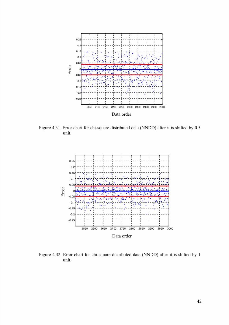
8/22/2019 Development of Univariate Control Chart for Non Normal Data
http://slidepdf.com/reader/full/development-of-univariate-control-chart-for-non-normal-data 54/87
42
2050 2100 2150 2200 2250 2300 2350 2400 2450 2500
-0.25
-0.2
-0.15
-0.1
-0.05
0
0.05
0.1
0.15
0.2
0.25
Figure 4.31. Error chart for chi-square distributed data (NNDD) after it is shifted by 0.5
unit.
2550 2600 2650 2700 2750 2800 2850 2900 2950 3000
-0.25
-0.2
-0.15
-0.1
-0.05
0
0.05
0.1
0.15
0.2
0.25
Figure 4.32. Error chart for chi-square distributed data (NNDD) after it is shifted by 1
unit.
Data order
Data order
E r r o r
E r r o r

8/22/2019 Development of Univariate Control Chart for Non Normal Data
http://slidepdf.com/reader/full/development-of-univariate-control-chart-for-non-normal-data 55/87
43
-5 0 5 10 15 20 250
0.02
0.04
0.06
0.08
0.1
0.12
0.14
0.16
0.18
0.2
Figure 4.33. Plots of ksdensity and chi-square probability density function (chi2pdf )after the process is returned back to in-control situation. Wavy line
indicates the ksdensity estimate while the other smooth line shows pdf.
3100 3200 3300 3400 3500 3600 3700 3800 3900 4000-0.1
-0.08
-0.06
-0.04
-0.02
0
0.02
0.04
0.06
0.08
0.1
Figure 4.34. Error chart for chi-square distributed data (NNDD) after the process is
returned back to in-control situation.
Sample quality characteristic
Data order
R e l a t i v e f r e u e n c
E r r o r

8/22/2019 Development of Univariate Control Chart for Non Normal Data
http://slidepdf.com/reader/full/development-of-univariate-control-chart-for-non-normal-data 56/87
44
4.3. Results of OM and NM for Industrial Data
Non-normally distributed industrial data that was described in section 3.1.3
was used to plot the control charts. OM and the NM were used for this non-normallydistributed industrial data (NND-ID) as well. The histogram for this data for in-control
situation is shown in Figure 3.4. The NND-ID used in this study looked non-normal and
skewed to the right. The same result was clear from Figure 3.5 where the normal
probability plot of the NND-ID is given. The diagonal red line on the figure shows the
conformity to normal distribution and any deviation from this line is an indication of
non-normality.
4.3.1. Application of OM for α = 0.01
The Shewhart control chart (OM) is shown in Figure 4.35. As can be seen from
the figure, the data is obviously non-normally distributed and there are several data
points that are outside of the control limits. These violations are unevenly distributed.
There is only one violation below the LCL when all other violations are located above
the UCL. This confirmed that the Shewhart control charts cannot be used for NND-ID.
Therefore, a new method is necessary for monitoring such industrial data.
OM was applied to the out of control part of the industrial data and the results
are given in Figure 4.36. The OM appears to successfully identify the out of control
situation. But this was observed only above the UCL line, there was no violation below
the LCL line.
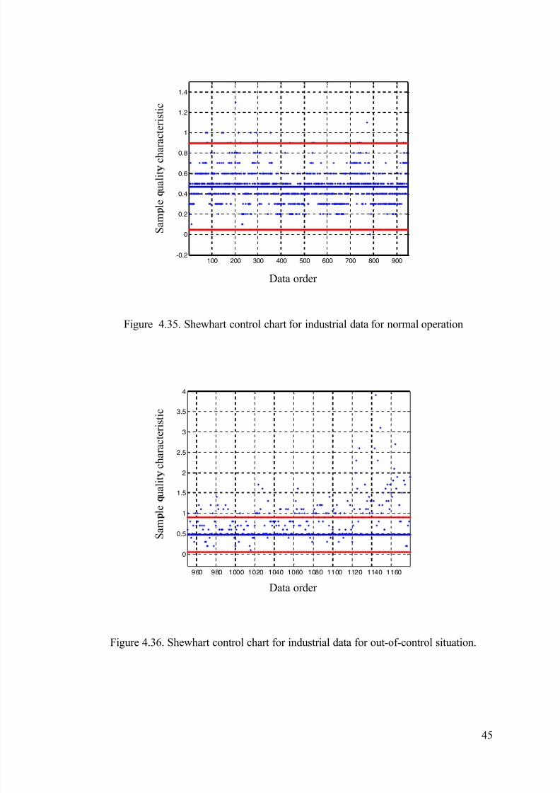
8/22/2019 Development of Univariate Control Chart for Non Normal Data
http://slidepdf.com/reader/full/development-of-univariate-control-chart-for-non-normal-data 57/87
45
100 200 300 400 500 600 700 800 900-0.2
0
0.2
0.4
0.6
0.8
1
1.2
1.4
Figure 4.35. Shewhart control chart for industrial data for normal operation
960 980 1000 1020 1040 1060 1080 1100 1120 1140 1160
0
0.5
1
1.5
2
2.5
3
3.5
4
Figure 4.36. Shewhart control chart for industrial data for out-of-control situation.
Data order
Data order
S a m
l e
u a l i t c
h a r a c t e r i s t i c
S a m
l e
u a l i t c
h a r a c t e r i s t i
c
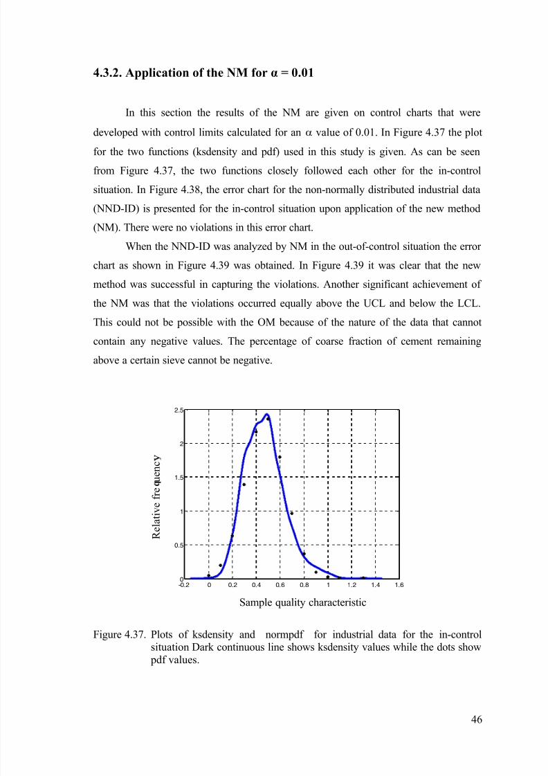
8/22/2019 Development of Univariate Control Chart for Non Normal Data
http://slidepdf.com/reader/full/development-of-univariate-control-chart-for-non-normal-data 58/87
46
4.3.2. Application of the NM for α = 0.01
In this section the results of the NM are given on control charts that were
developed with control limits calculated for an α value of 0.01. In Figure 4.37 the plotfor the two functions (ksdensity and pdf) used in this study is given. As can be seen
from Figure 4.37, the two functions closely followed each other for the in-control
situation. In Figure 4.38, the error chart for the non-normally distributed industrial data
(NND-ID) is presented for the in-control situation upon application of the new method
(NM). There were no violations in this error chart.
When the NND-ID was analyzed by NM in the out-of-control situation the error
chart as shown in Figure 4.39 was obtained. In Figure 4.39 it was clear that the new
method was successful in capturing the violations. Another significant achievement of
the NM was that the violations occurred equally above the UCL and below the LCL.
This could not be possible with the OM because of the nature of the data that cannot
contain any negative values. The percentage of coarse fraction of cement remaining
above a certain sieve cannot be negative.
-0.2 0 0.2 0.4 0.6 0.8 1 1.2 1.4 1.60
0.5
1
1.5
2
2.5
Figure 4.37. Plots of ksdensity and normpdf for industrial data for the in-controlsituation Dark continuous line shows ksdensity values while the dots show
pdf values.
Sample quality characteristic
R e l a t i v e f r e u e n c
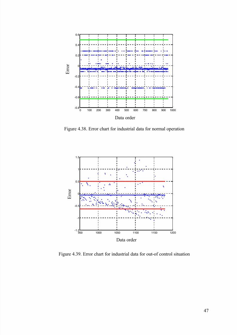
8/22/2019 Development of Univariate Control Chart for Non Normal Data
http://slidepdf.com/reader/full/development-of-univariate-control-chart-for-non-normal-data 59/87
47
0 100 200 300 400 500 600 700 800 900 1000-0.8
-0.6
-0.4
-0.2
0
0.2
0.4
0.6
Figure 4.38. Error chart for industrial data for normal operation
950 1000 1050 1100 1150 1200-1.5
-1
-0.5
0
0.5
1
1.5
Figure 4.39. Error chart for industrial data for out-of control situation
Data order
Data order
E r r o r
E r r o r
8/22/2019 Development of Univariate Control Chart for Non Normal Data
http://slidepdf.com/reader/full/development-of-univariate-control-chart-for-non-normal-data 60/87
48
CHAPTER 5
CONCLUSIONS AND RECOMMENDATIONS FOR
FUTURE STUDY
For normally distributed data (NDD) both methods (OM and NM) worked
well for in-control situation. The OM contained a total of six false alarms while the NM
had none. This is a burden on the OM because run rules must be created to determine
whether the alarm signals are a part of an out-of-control situation or just assignable
causes (Montgomery 2005). The NM removes this necessity and hence is more
practical. The effects of shifts to mimic an out-of-control situation showed a gradual
increase in the number of violations in both methods. Upon feeding in-control data both
methods could be returned back to in-control status from out-of-control case.
Non-normally distributed data NNDD were used to test performance of both OM
and NM. For in-control case the OM was found to be unsuccessfull by causing a large
number of violations. When changes to mean and standard deviation introduced, the
OM was found to be insensitive and unable to capture such conditions. On the other
hand, the NM was found to be successful in both the in-control and out-of-control cases.
Small amounts of shifts (i.e. less than 0.01) could be quickly captured by the NM. The
NM could also be easily returned back to normal operation by feeding in-control data.
ID were first tested for its underlying distribution and it was identified as an
NNDD. Then both OM and NM were applied for the in-control case and several false
violations were observed in the OM while the NM worked well without violations.
When the out-of-control data were analyzed by OM and NM, the OM was found to
provide violations that were all located above the UCL. This one-sided biased result
was expected because of the type of the distribution. The NM, however, was very well
in that regard. The violations occurred equally balanced above the UCL and below the
LCL. The NM was successfully implemented and the task outlined in the aim of the
study part (section 2.1.3) was achieved.
The approach of this study was mainly aimed at developing a control chart for
non-normal data, not on the economic aspects of such NND processes.
More NND-ID must be collected to further check and confirm the utility of the
NM. The author is optimistic that this would yield good results for better process

8/22/2019 Development of Univariate Control Chart for Non Normal Data
http://slidepdf.com/reader/full/development-of-univariate-control-chart-for-non-normal-data 61/87
49
control. The effects of varying smoothing parameters, shift ratios and sample sizes can
be tested. Care must be taken to collect ID with higher measurement precision. New
method’s performance can be compared against other methods based on ARL and ATS
criteria.

8/22/2019 Development of Univariate Control Chart for Non Normal Data
http://slidepdf.com/reader/full/development-of-univariate-control-chart-for-non-normal-data 62/87
50
REFERENCES
Alexander, S. M., Dillman M. A., Usher, J. S., Damodaran, B. 1995. “Economic design
of control charts using the Taguchi loss function,” Computers and Industrial
Engineering. Vol. 28, pp. 671-679.
Amin, R., Reynolds, M. R. Jr., Bakir, S. T. 1995. “Nonparametric quality control charts based on the sign statistic,” Communications in Statistics. Vol. 24, pp.1597-
1623.
Abramowitz, M. and Stegun, I. A. 1964. “Handbook of Mathematical Functions,”
26.1.26.
Bakir, S.T. 2004. “A Distribution-Free Shewhart Quality Control Chart Based on
Signed-Ranks,” Quality Engineering. Vol. 16, pp.613-623.
Bai, D.S. and Choi, I.S. 1995. “ X and R control charts for skewed populations,”
Journal of Quality Technology. Vol. 27, pp. 120-131.
Bowman, A.W. and Azzalini, A.x1997. “ Applied Smoothing Techniques for Data
Analysis,” Oxford University.
Burr, I.W. 1942. “Cumulative frequency distribution. Annals of MathematicalStatistics,” Vol.13, pp. 215-232.
Burr, I. W. 1967. “The effect of nonnormality on constants for X and R charts,”
Industrial Quality Control. pp. 563–569.
Chang, Y.S., Bai, D.S. 2001. « Control charts for positively skewed populations with
weighted standard deviations,” Quality and Reliability Engineering
International. Vol. 17, pp.397-406.
Chen, Y.K. 2004. “Economic design of control charts for non-normal data usingvariable sampling policy,” International Journal of Production Economics. Vol.
92, pp. 61-74.
Chiu, W.K. 1975. “Economic design of attribute control charts,” Technometrics. Vol.
17, pp.81-87.
Chou, C.Y.; Chen, C.H.; Liu, H.R. 2000. “Economic-Statistical Design of X Charts for
Non-Normal Data by Considering Quality Loss,” Journal of Applied Statistics.
Vol. 27, pp. 939- 951.
Chou, C.Y.; Chen, C.H.; Liu, H.R. 2004. “Effect of Nonnormality on the Economic
Design of Warning Limit X Charts,” Quality Engineering. Vol. 16, pp. 567-575.

8/22/2019 Development of Univariate Control Chart for Non Normal Data
http://slidepdf.com/reader/full/development-of-univariate-control-chart-for-non-normal-data 63/87
51
Chou, C. Y. and Cheng, P.H. 1997. “Ranges control chart for non-normal data,” Journal
of the Chinese. Vol. 14, pp. 401-409.
Chou, C.Y.; Li, M.H.C.; Wang, P.H. 2001. “Economic Statistical Design of Averages
Control Charts for Monitoring a Process under Non-normality,” The
International Journal of Advanced Manufacturing Technology. Vol. 17, pp. 603-609.
Dou, Y. and Ping, S. 2002. “One Sided Control Charts for The Mean of PositivelySkewed Distributions,” The Quality Management. Vol. 13, pp. 1021-1033.
Duncan, A. J. 1956. “The economic design of x charts used to maintain current control
of a process,” Journal of the American Statistical Association. Vol. 51, pp. 228-
242.
Montgomery, Douglas C.2005.“Introduction to Statistical Quality Control”,5th
edition,Wiley &Sons,Inc.
Rahim, M. A. 1985. “Economic model of x chart under non-normality and measurementerrors,” Computers and Operations Research. Vol.12, pp. 291-299.
Reynolds Jr, M.R., Amin, R.W., Arnold, J.C., Nachlas, J.A. 1988. “Charts with variable
sampling interval,” Technometrics. Vol 30, pp. 181-192.
Saniga , E. M. and Shirland, L. E. 1977. “Quality control in practice: a survey”, Quality
Progress. Vol. 10, pp. 30-33.
Saniga, E. M. 1989. “Economic statistical control chart designs with an application to x
and R charts,” Technometrics. Vol. 31, pp. 313-320.
Shewhart, W.A. 1931. “Economic Control of Quality of Manufactured Product ,” NewJersey.
Tasi, H. T. 1990. “Probabilistic tolerance design for a subsystem under Burr Distribution using Taguchi’s quadratic loss function,” Communications in
Statistics. Vol. 19, pp. 4679-4696.
Yourstone, S. A. and Zimmer, W. J. 1992. “Non-normality and the design of controlcharts for averages,” Decision Sciences. Vol. 23, pp. 1099-1113.
Woodall, W. H. 1985. “The statistical design of quality control charts”, The Statistician.Vol. 34, pp. 155-160.

8/22/2019 Development of Univariate Control Chart for Non Normal Data
http://slidepdf.com/reader/full/development-of-univariate-control-chart-for-non-normal-data 64/87
52
APPENDICES
APPENDIX A
Normally Distributed Data19.5674 20.7143 17.8293 19.7041 20.5690 20.6565 19.4535 17.9457
18.3344 21.6236 19.9408 18.5249 19.1783 18.8322 19.1532 20.1326
20.1253 19.3082 18.9894 19.7660 19.7344 19.5394 19.7537 21.5929
20.2877 20.8580 20.6145 20.1184 18.8122 19.7376 20.6630 21.0184
18.8535 21.2540 20.5077 20.3148 17.7977 18.7868 19.1458 18.4196
21.1909 18.4063 21.6924 21.4435 20.9863 18.6806 18.7987 19.9213
21.1892 18.5590 20.5913 19.6490 19.4814 20.9312 19.8801 19.3183
19.9624 20.5711 19.3564 20.6232 20.3274 20.0112 19.9347 18.9754
20.3273 19.6001 20.3803 20.7990 20.2341 19.3549 20.4853 18.7656
20.1746 20.6900 18.9909 20.9409 20.0215 20.8057 19.4045 20.2888
19.8133 20.8156 19.9805 19.0079 18.9961 20.2316 19.8503 19.5707
20.7258 20.7119 19.9518 20.2120 19.0529 19.0102 19.5652 20.0558
19.4117 21.2902 20.0000 20.2379 19.6256 21.3396 19.9207 19.6321
22.1832 20.6686 19.6821 18.9922 18.8141 20.2895 21.5352 19.5350
19.8636 21.1908 21.0950 19.2580 18.9441 21.4789 19.3935 20.3710
20.1139 18.7975 18.1260 21.0823 21.4725 21.1380 18.6526 20.7283
21.0668 19.9802 20.4282 19.8685 20.0557 19.3159 20.4694 22.1122
20.0593 19.8433 20.8956 20.3899 18.7827 18.7081 19.0964 18.6427
19.9044 18.3959 20.7310 20.0880 19.9588 19.9271 20.0359 18.9774
19.1677 20.2573 20.5779 19.3645 18.8717 19.6694 19.3725 21.0378
20.2944 18.9435 20.0403 19.4404 18.6507 19.1564 20.5354 19.6102
18.6638 21.4151 20.6771 20.4437 19.7389 20.4978 20.5529 18.6187
19.0781 19.1949 20.5689 19.0501 20.9535 19.0224 19.5532 21.0821
20.3155 20.5287 19.7444 20.7812 21.2781 21.4885 19.7963 20.1286
21.5532 20.2193 19.6225 19.2879 19.4522 20.1068 20.3271 19.243820.7079 19.8868 18.8929 19.9887 20.2608 21.8482 19.3270 19.9109
21.9574 20.3792 20.4855 19.9992 19.9868 19.7249 19.8507 17.9911
20.5045 20.9442 19.9950 19.7506 19.4197 22.2126 17.5510 21.0839
21.8645 17.8796 19.7238 20.3966 22.1363 21.5085 20.4733 19.0188
19.6602 19.3553 21.2765 19.7360 19.7424 18.0549 20.1169 19.3115
18.8602 19.2957 21.8634 18.3360 18.5905 18.3195 19.4089 21.3395
19.7889 18.9819 19.4774 18.9710 21.7701 19.4265 19.3453 19.0908
21.1902 19.8179 20.1034 20.2431 20.3255 19.8142 18.9193 19.5871
18.8838 21.5210 19.1924 18.7434 18.8810 20.0089 19.9523 19.493820.6353 19.9616 20.6804 19.6528 20.6204 20.8369 20.3793 21.6197

8/22/2019 Development of Univariate Control Chart for Non Normal Data
http://slidepdf.com/reader/full/development-of-univariate-control-chart-for-non-normal-data 65/87
53
19.3986 21.2274 17.6354 19.0586 21.2698 19.2777 19.6696 20.0809
20.5512 19.3038 20.9901 18.8254 19.1040 19.2785 19.5001 18.9189
18.9002 20.0075 20.2189 18.9789 20.1352 19.7988 19.9640 18.8755
20.0860 19.2171 20.2617 19.5983 19.8610 19.9795 19.8252 21.7357
17.9954 20.5869 21.2134 20.1737 18.8366 20.2789 19.0427 21.937519.5069 19.7488 19.7253 19.8839 21.1837 21.0583 21.2925 21.6351
20.4620 20.4801 19.8669 21.0641 19.9846 20.6217 20.4409 18.7441
19.6790 20.6682 18.7295 19.7546 20.5362 18.2494 21.2809 19.7865
21.2366 19.9217 18.3364 18.4825 19.2836 20.6973 19.5023 19.8011
19.3687 20.8892 19.2964 20.0097 19.3444 20.8115 18.8813 20.3075
17.6748 22.3093 20.2809 20.0714 20.3144 20.6363 20.8076 19.4277
18.7684 20.5246 19.4588 20.3165 20.9131 21.3101 20.0412 19.7334
21.0556 19.9882 18.6665 19.8986 17.3650 20.0281 19.1237 19.7345
19.5124 20.8564 18.6546 20.4998 20.0559 22.3726 20.2293 20.7017
21.8625 20.2685 21.4819 19.1095 20.9443 19.2663 21.7513 19.4573
21.1069 20.6250 20.0327 20.1391 17.5760 19.9355 20.7532 20.9122
18.7724 18.9527 21.8705 19.7639 19.7762 18.5560 20.0650 19.8279
19.3301 21.5357 18.7910 19.9245 20.0581 20.6123 19.7072 19.6640
21.3409 20.4344 19.2174 19.6414 19.5754 18.6765 20.0828 20.5415
20.3881 18.0829 19.2327 17.9224 19.7971 19.3384 20.7662 20.9321
20.3931 20.4699 19.8928 19.8565 18.4869 19.8539 22.2368 19.4297
18.2927 21.2744 19.0229 21.3933 18.8736 20.2481 20.3269 18.5014
20.2279 20.6385 19.0360 20.6518 19.1850 19.9234 20.8633 19.9497
20.6856 21.3808 17.6208 19.6229 20.3666 21.7382 20.6794 20.5530
19.3632 21.3198 19.1618 19.3386 19.4139 21.6220 20.5548 20.0835
18.9974 19.0906 20.2573 20.2490 21.5374 20.6264 21.0016 21.5775
19.8144 17.6944 19.8162 19.6165 20.1401 20.0918 21.2594 19.6692
18.9460 21.7887 19.8324 19.4715 18.1372 19.1924 20.0442 20.7952
19.9285 20.3908 19.8830 20.0554 19.5458 19.5387 19.6859 19.2152
20.2792 20.0203 20.1685 21.2538 19.3479 18.5940 20.2267 18.7369
21.3733 19.5940 19.4988 17.4800 20.1033 19.6255 20.9967 20.6667
20.1798 18.4651 19.2949 20.5849 19.7794 19.5291 21.2159 21.5783
19.4580 20.2214 20.5082 18.9919 19.7210 17.5854 19.6724 18.8918
21.6342 18.6255 19.5791 18.6074 19.7226 19.3057 18.8418 19.9741
20.8252 19.1607 20.2291 18.6994 18.7063 18.6086 20.5801 18.8894
20.2308 19.7914 19.0405 19.3950 19.1116 20.3296 20.2398 20.7508
20.6716 20.7559 19.8540 18.5114 19.0135 20.5985 19.6491 20.5002
19.4919 20.5080 20.1319 20.2801 19.0172 19.0559 19.9869 20.3543
19.4408 20.3757 20.7445 20.5585 19.9284 20.1472 20.8921 19.4827
19.2466 19.0470 20.0755 20.3253 20.9778 21.4419 20.1733 19.8396
20.9258 20.7782 19.4734 19.6649 20.0183 20.6723 20.9232 18.9164
19.7515 19.9937 19.3145 19.6776 20.8180 20.1387 19.8214 18.045819.8502 20.5245 19.7316 19.6176 20.7023 19.1405 19.4783 19.0905

8/22/2019 Development of Univariate Control Chart for Non Normal Data
http://slidepdf.com/reader/full/development-of-univariate-control-chart-for-non-normal-data 66/87
54
18.7416 21.3643 18.8117 19.0466 19.7687 19.2477 21.4320 19.9944
20.3126 20.4820 20.2486 20.2336 19.8863 21.2296 19.1299 18.2765
22.6903 19.2129 20.1025 21.2352 20.1279 21.1508 20.8075 21.2631
20.2897 20.7520 19.9590 19.4215 19.2006 19.3920 19.4894 19.3996
18.5772 19.8331 17.7524 19.4985 19.7614 20.8062 20.7435 17.936120.2468 19.1838 19.4892 20.7229 19.9105 20.2171 20.8479 20.1109
18.5642 22.0941 20.2492 20.0395 18.9767 19.6265 19.1701 21.4876
20.1486 20.0802 20.3692 21.5413 20.9375 19.1680 20.5330 20.0530
18.3069 19.0627 20.1792 18.2989 18.8683 20.2869 21.0328 20.1620
20.7192 20.6357 19.9627 18.9663 19.2893 18.1811 18.9480 19.9731
21.1418 21.6820 18.3967 19.2363 18.8305 18.4269 20.3621 20.1736
21.5519 20.5936 20.3394 22.1764 21.0654 22.0157 19.9632 20.8822
21.3836 20.7902 19.8689 20.4316 19.3196 19.9280 18.7724 20.1823
19.2419 20.1053 20.4852 19.5562 18.2742 22.6289 19.7249 20.7553
20.4427 19.8414 20.5988 20.0300 20.8132 19.7567 20.2137 20.2349
20.9111 20.8709 19.9140 19.6843 22.7316 20.4995 19.5995 19.4022
18.9259 19.8052 19.1053 20.4194 20.4111 19.4892 20.0649 20.0208
20.2018 21.3242 20.8121 21.1911 18.6931 20.7712 18.2420 20.8261
20.7629 19.8735 20.1095 20.8584 20.3838 17.3558 21.6867 19.9919
18.7118 19.2628 19.2245 20.2710 21.3059 18.9477 20.6256 20.1098
18.3455 19.3081 20.7748 21.2315 21.3171 20.2854 20.3274 18.8670
19.0096 20.6802 20.2450 19.0740 20.2280 19.8206 18.3534 19.3169
20.6852 18.9275 20.1650 19.8881 18.5704 18.5329 20.4287 19.7221
19.0251 20.8998 20.4062 19.1970 19.8503 21.3953 19.2628 20.6548
19.3933 17.8769 21.2160 18.3350 19.4950 20.4408 20.5649 18.7516
20.6868 20.2847 21.4484 19.0986 18.2709 20.5654 18.6158 19.4025
20.0200 19.2667 18.9749 20.5883 19.5825 19.3064 20.4603 19.5182
21.0638 19.2266 20.2054 20.5542 19.3850 20.8339 20.6294 20.9834
18.6590 20.1518 20.5889 19.5848 20.7208 17.7626 20.3798 21.7621
20.4795 19.6632 19.7360 20.0618 20.3394 21.0976 18.9867 21.4274
18.3660 20.9708 22.4953 20.4574 20.8828 19.9984 19.6528 20.9118
18.5573 19.8928 20.8559 20.1990 20.2842 18.3854 20.4419 20.3268
20.2938 21.0135 19.1490 20.2576 19.8545 18.7713 18.4098 20.0696
19.8596 19.5247 20.8119 22.0807 19.9104 20.2074 19.2986 18.5002
18.8697 20.0689 20.7002 17.7228 20.2892 20.2209 18.9224 19.5818
19.7075 20.3986 20.7599 20.3390 21.1648 18.9939 21.0022 19.9790
19.4175 21.1163 18.2871 20.2899 20.8057 19.5469 21.7295 20.2284
19.1037 20.6205 21.5370 20.6623 18.6444 21.3995 20.7090 18.9918
20.2486 19.7123 18.3902 19.4191 20.1209 19.5380 19.2521 19.3354
18.5103 18.6282 21.1095 20.8878 19.7778 20.0327 20.2289 20.5582
20.3135 19.3141 18.8903 20.1719 20.5717 20.7988 19.7765 18.8115
17.9749 20.3317 20.3855 20.8488 19.6999 20.8968 19.1467 20.858520.5290 19.0023 20.9652 20.9638 21.1343 20.1379 20.3456 17.8947
8/22/2019 Development of Univariate Control Chart for Non Normal Data
http://slidepdf.com/reader/full/development-of-univariate-control-chart-for-non-normal-data 67/87
55
20.3435 20.2914 20.8183 21.3219 21.5350 18.3809 19.3978 18.5861
20.7582 19.7933 19.5744 20.4938 19.1291 20.0798 19.4784 19.6157
20.5536 21.1071 20.0370 19.9357 19.2024 19.6865 21.2591
19.5421 19.6391 19.7085 19.6988 18.4114 21.0943

8/22/2019 Development of Univariate Control Chart for Non Normal Data
http://slidepdf.com/reader/full/development-of-univariate-control-chart-for-non-normal-data 68/87
56
APPENDIX B
Non-Normally Distributed Data
3.1806 4.2753 1.9871 8.4224 3.5193 2.0197 2.7189 0.54581.0469 3.8881 6.4056 0.8265 1.2798 4.9880 2.8859 7.9339
4.7129 1.1187 6.0065 5.7200 3.6803 5.0720 5.7750 2.9788
5.2366 5.1358 11.4692 7.5410 4.6915 1.9921 2.0953 5.3703
1.7586 1.9079 6.3175 6.8611 5.3277 2.4953 7.0639 5.0595
8.8698 9.9771 2.7014 6.2668 10.1234 8.3642 6.2334 4.3968
8.8615 2.3691 5.5522 4.4531 3.3800 3.9576 2.3365 1.9988
4.2235 6.0837 1.9897 6.6479 6.4392 5.5854 3.5975 2.1003
5.3700 5.0116 4.2761 6.2332 7.1370 4.5976 1.6928 5.9248
4.8681 2.1465 4.1929 3.6235 7.7353 2.2940 6.5930 2.80603.8066 0.5696 4.3335 3.3144 5.2427 5.9701 2.2737 3.9075
6.8404 4.1614 3.4633 1.6532 10.3081 10.3584 1.6716 3.1753
2.8219 3.3219 1.4513 7.6935 8.6212 2.9154 3.9899 4.1040
14.4616 1.6958 3.6092 4.3665 2.6152 2.2880 6.1669 10.6059
3.9441 1.9089 7.7899 2.6980 1.5342 8.1630 1.8350 2.7819
4.6775 10.2743 4.7232 7.1645 4.1222 3.2841 4.5914 4.5001
8.2936 4.4995 6.5675 5.0516 1.9628 1.4063 0.7056 1.8230
4.5102 1.6468 1.7244 2.0238 1.6206 5.3302 3.0378 5.9255
4.0578 4.2131 3.1139 10.9179 5.2404 10.7029 5.8409 4.31862.3158 2.7360 3.7609 8.0761 3.1884 6.7692 3.4554 3.5700
5.2591 6.1083 0.6628 1.1472 4.4997 13.0274 9.0882 9.2820
1.4699 6.1733 4.7354 4.1059 3.3381 5.9948 2.7279 2.9698
6.7948 5.2139 4.3002 3.6016 3.1036 12.4662 0.4599 7.3749
11.0856 2.9274 4.3309 1.0487 5.5197 3.4080 1.6248 5.1728
2.5992 1.4737 3.6397 1.9551 6.8504 1.7695 8.2432 6.4459
7.3818 8.3205 5.6088 5.0891 13.9997 3.7410 4.0085 1.9235
9.1726 2.5569 1.8670 1.5869 1.4399 8.8666 5.5484 10.6087
1.1311 1.0299 4.1943 3.3895 1.9662 6.4855 7.7497 5.74221.3249 2.8547 5.5488 2.1108 3.0075 2.7930 0.6087 0.7851
6.2416 3.8090 3.4317 1.7137 11.0646 1.6310 2.6990 5.8692
3.2595 4.3597 3.0220 1.9687 4.5759 2.6453 2.5730 9.2717
6.6986 7.2937 4.2283 3.2552 1.8663 9.6010 1.9740 6.4981
7.2053 2.5358 3.8389 4.8650 1.7943 5.5792 3.8191 9.8018
6.7852 2.5375 2.0820 4.0004 11.7145 5.5965 10.5305 9.4959
9.3496 3.7676 9.3609 8.2816 12.9055 1.0000 4.2212 2.1696
6.6147 4.2734 5.7653 3.6503 11.1491 5.0393 9.0443 0.4729
8.8694 5.2073 9.3040 1.2252 1.5878 6.6814 2.5899 12.0203
1.6698 8.2552 3.0270 4.3621 3.7346 2.7160 4.3555 5.5886
8/22/2019 Development of Univariate Control Chart for Non Normal Data
http://slidepdf.com/reader/full/development-of-univariate-control-chart-for-non-normal-data 69/87
57
4.6450 6.4332 1.8038 4.5469 3.7737 2.0012 2.4130 4.3934
2.3640 0.9528 7.1724 5.3336 5.3031 3.8095 6.3011 3.2447
6.6610 6.7275 4.4558 5.9776 2.8574 1.9121 3.6351 1.2034
0.4344 7.1882 2.4666 9.2900 2.0454 4.1261 5.9061 5.0183
7.9506 6.4896 4.0762 2.9124 3.1466 5.2083 6.6130 1.41585.0102 9.4475 0.7018 5.1474 8.3633 9.7637 4.1068 2.4442
5.1502 5.3694 8.3716 4.2947 15.7433 4.8846 7.5134 4.0253
8.9772 2.6387 2.0391 2.8397 5.0440 2.9255 15.3066 2.0464
3.5740 3.9084 2.6061 14.1556 3.5949 11.1443 6.0686 2.0699
3.9531 5.8813 9.5937 3.6183 6.7446 7.2450 4.2987 0.4252
1.5660 4.6868 2.1699 1.3674 3.0506 5.0488 7.6157 2.3045
1.0492 2.8157 3.2280 11.9123 12.4540 6.6265 4.3147 5.1359
2.5746 2.6776 3.6057 5.3641 8.4768 3.0031 6.0680 3.8144
5.0435 3.7630 11.0769 6.4282 3.4176 2.5938 9.7182 3.8584
2.0780 1.2309 6.4515 9.2494 6.1309 1.3923 5.9130 3.9980
3.9175 1.7913 4.6093 2.1945 7.6974 5.3780 2.4047 4.8485
6.9155 2.3496 2.3641 4.7436 2.8620 6.3450 6.9456 3.0190
2.2049 5.5047 3.1121 3.9368 1.2494 4.7812 3.8604 2.5714
4.7557 2.8268 1.3722 1.7315 4.1868 4.0415 2.3472 6.0081
3.6747 4.7589 3.3216 8.8357 6.1738 4.4164 13.8836 3.2085
4.1150 0.8375 3.0896 4.2881 4.5838 2.2316 4.5736 3.3023
3.3611 3.1290 11.8040 6.1114 10.8340 3.5978 2.1183 2.0890
0.6433 2.6832 6.9505 2.5479 3.4307 3.4387 6.4873 5.0580
3.9243 4.6447 4.5275 2.6757 7.1210 1.7397 11.4107 9.0819
9.8656 3.7157 3.5273 5.3262 2.4092 6.2751 6.3264 2.8436
6.5494 3.5627 4.5818 4.6555 1.5770 5.0782 7.1005 3.0182
3.3152 2.5125 7.0029 12.3693 6.6071 3.3803 4.6506 6.8287
2.6632 4.1461 14.8173 3.5729 1.3906 7.5259 3.8831 4.4507
5.1083 1.3209 5.3687 14.6556 1.5215 10.8383 7.4361 10.6387
3.2995 6.3975 7.4041 10.4642 2.7851 1.8212 3.7849 1.0069
2.9563 1.4882 6.6569 2.6204 1.2623 4.2574 4.5593 1.9469
4.4984 2.6629 6.1803 4.4646 6.1944 1.8171 2.9605 2.4515
9.1715 3.9173 8.0015 3.4728 3.5670 6.9409 2.6124 14.4172
6.2932 5.1055 1.7217 5.0356 1.5316 5.9789 3.5903 5.7322
1.9916 4.1116 8.2875 7.9796 2.2088 2.9820 1.6919 3.1538
7.7501 11.7288 2.6231 8.9890 2.0296 2.8867 5.1071 4.4222
0.3977 1.7881 0.9797 2.9240 4.1259 2.4723 4.6420 3.4689
3.7072 7.1719 7.1953 7.6118 0.4034 7.6702 4.2137 7.8965
4.5065 2.9972 10.1149 3.8461 7.8655 3.6421 0.5130 4.3874
3.1996 6.9114 6.6290 2.8009 4.0252 3.9070 2.9969 7.2149
2.2635 7.3394 4.7545 4.3948 8.0541 1.5841 5.1093 6.7473
2.4746 2.3206 0.7507 5.6891 3.0792 5.3204 5.5136 3.6875
9.0547 6.0994 2.1695 8.8707 4.5395 18.0582 4.8826 4.0072
8/22/2019 Development of Univariate Control Chart for Non Normal Data
http://slidepdf.com/reader/full/development-of-univariate-control-chart-for-non-normal-data 70/87
58
8.6806 8.1406 4.3169 7.0233 5.6159 5.2433 4.2245 4.7210
2.7785 1.9155 0.9822 0.2798 8.5205 1.3493 1.1196 2.3803
7.1662 5.4892 9.2167 5.2291 6.4286 5.1012 5.4112 3.6682
5.0045 4.2259 2.7952 7.2486 3.5404 1.3319 3.9586 4.0753
3.3243 1.6309 4.6681 4.3095 1.4195 4.7856 5.9244 1.9651
2.3164 3.5729 10.3538 7.3836 2.6116 1.0158 6.3458 7.7208
5.2339 3.8780 4.4912 7.0379 5.3850 6.8141 4.0850 1.7826
0.8814 1.8621 4.8279 9.4270 2.0098 8.6386 5.3632 2.5597
13.3880 6.6600 4.2547 9.0638 5.2491 10.6959 3.4197 7.3732
4.1249 1.8807 4.8647 7.8122 8.4778 9.8162 3.4517 2.2799
17.5944 7.5586 7.4837 1.0596 5.0952 2.4628 1.9618 7.1898
3.6558 0.6065 4.8925 2.0227 4.8374 5.7715 4.9666 6.7390
4.8637 5.2267 6.9589 6.6798 5.6426 7.6070 6.3084 6.9776
7.6590 2.5132 6.0076 2.0504 8.9893 1.8781 3.6016 0.9938
3.8287 2.4320 4.7333 2.7814 10.1489 4.9549 16.6123 10.61592.9718 4.7959 5.2113 6.6860 7.8413 6.9895 2.1389 1.1119
10.0637 3.4154 2.0361 4.3926 7.2163 1.5397 4.0121 8.4891
2.2434 6.5900 2.1059 8.2801 4.4433 2.0898 2.3731 1.8186
6.3064 2.8384 4.2950 1.4630 5.0399 7.0516 1.0476 5.5701
6.1780 7.5074 5.4624 5.9038 1.3401 5.4111 2.1845 3.8265
3.2224 4.8593 2.1970 1.0834 3.9074 7.4866 7.1645 1.2904
4.5178 7.3433 7.1908 1.3227 3.0103 5.2251 1.4422 9.8758
5.8243 7.8349 4.6639 5.2570 0.9760 3.9188 4.6991 5.7650
4.9460 9.5062 18.3754 3.9331 3.2169 4.0747 3.7116 6.2200
5.1366 4.1467 5.6597 1.7848 2.7633 5.2416 6.2438 7.2809
13.7985 9.4820 1.5123 3.5279 6.8204 8.7466 3.5084 2.3024
5.4100 1.1008 5.5643 2.8347 2.6173 3.2150 8.6037 3.7477
5.2440 1.0687 5.9764 2.1939 3.5657 4.2717 2.9720 6.9614
0.5203 5.7219 2.9968 5.1072 6.5609 5.0412 1.3615 5.5363
8.4345 2.5052 5.0624 1.2609 1.5992 1.9914 3.2976 1.4567
4.3286 6.2183 9.1987 5.3234 2.8015 2.6564 3.1202 10.3236
1.1062 1.4023 1.8721 6.0846 3.0640 6.1930 3.5307 4.4304
1.6292 5.8345 8.0041 5.4252 7.9208 1.6916 3.5057 12.5015
4.9730 6.4628 11.6792 6.9706 11.8663 2.4278 1.1373 1.65975.0169 5.5505 6.7738 2.5988 10.0402 5.1812 8.4191 2.4135
1.9951 1.9824 2.4834 7.3838 7.6098 10.6049 9.5174 4.9934
3.1317 3.3894 5.0426 0.6208 5.3684 1.9151 3.9716 3.2579
9.8968 5.7688 3.7081 3.3552 4.5415 6.4481 2.5053 4.5273
3.1107 1.1353 2.2755 6.1758 1.2479 2.3838 4.1439 0.9449
4.4304 2.5790 5.4325 1.1766 3.4311 3.4743 2.9004 11.4372
7.1359 10.9490 4.6646 3.7530 3.7986 2.7913 5.2721 5.3704
2.4921 0.6540 1.7804 3.1974 3.5044 9.1972 1.6325 6.8013
4.8730 7.8051 4.7521 5.9556 9.5943 3.6478 4.5726 1.4540
6.0804 2.9452 2.1851 2.2419 7.5460

8/22/2019 Development of Univariate Control Chart for Non Normal Data
http://slidepdf.com/reader/full/development-of-univariate-control-chart-for-non-normal-data 71/87
59
APPENDIX C
Industrial Data0.3 0.4 0.4 0.3 0.6 0.5 0.6 0.2 0.6 0.5 0.5 0.5 0.3 0.4 0.3 0.2
0.3 0.6 0.5 0.3 0.6 0.8 0.6 0.5 0.6 0.5 0.6 0.4 0.3 0.2 0.3 0.4
0.8 0.5 0.6 0.5 0.5 0.4 0.5 0.5 0.5 0.5 0.8 0.3 0.6 0.4 0.3 0.6
0.5 0.5 0.4 0.3 0.4 0.6 0.8 0.3 0.8 0.5 0.8 0.2 0.8 0.2 0.2 0.6
0.3 0.6 0.3 0.7 0.6 0.4 0.9 0.6 0.9 0.6 1.0 0.3 0.5 0.4 0.5 0.5
0.3 0.4 0.5 0.5 0.4 0.6 0.5 0.4 0.7 0.6 0.6 0.6 0.5 0.3 0.3 0.4
0.2 0.5 0.4 0.3 0.4 0.4 0.6 0.3 1.0 0.5 0.7 0.4 0.4 0.2 0.5 0.6
0.7 0.4 0.4 0.6 0.5 0.6 0.6 0.4 0.6 0.4 0.6 0.3 0.4 0.3 0.5 0.4
0.5 0.6 0.3 0.2 0.3 0.5 0.2 0.3 0.4 0.6 0.7 0.4 0.5 0.4 0.6 0.40.3 0.5 0.5 0.4 0.6 0.5 0.2 0.6 0.4 0.5 0.6 0.2 0.4 0.4 0.5 0.3
0.4 0.5 0.4 0.4 0.5 0.4 0.5 0.5 0.4 0.5 0.6 0.5 0.5 0.6 0.4 0.5
0.4 0.6 0.8 0.3 0.5 0.8 0.1 0.3 0.9 0.5 0.7 0.3 0.5 0.4 0.4 0.3
0.4 0.5 0.6 0.7 0.5 0.7 0.1 0.3 0.8 0.4 0.5 0.2 0.4 0.4 0.4 0.3
0.1 0.7 0.5 0.5 0.6 0.5 0.2 0.3 0.5 0.4 0.5 0.2 0.4 0.3 0.3 0.5
0.3 0.6 0.7 0.5 0.6 0.6 0.2 0.2 0.4 0.5 0.4 0.2 0.4 0.3 0.4 0.4
0.6 0.6 0.6 0.3 0.5 0.7 0.3 1.0 0.5 0.5 0.4 0.3 0.5 0.4 0.3 0.6
0.3 0.6 0.6 0.4 0.9 1.3 0.4 0.2 0.4 0.6 0.5 0.2 0.4 0.4 0.3 0.5
0.5 0.6 0.5 0.3 0.4 0.8 0.2 0.6 0.7 0.5 0.5 0.3 0.4 0.3 0.3 0.60.3 0.6 0.6 0.3 0.7 0.6 0.6 0.4 0.5 0.4 0.4 0.2 0.3 0.4 0.4 0.5
0.4 0.5 0.5 0.3 0.5 0.8 0.5 0.6 0.8 0.5 0.4 0.2 0.4 0.2 0.2 0.7
0.4 0.6 0.4 0.3 0.4 0.5 0.6 0.6 0.3 0.5 0.5 0.3 0.3 0.4 0.3 0.7
0.3 0.4 0.6 0.7 0.7 0.5 0.5 0.7 0.4 0.6 0.3 0.3 0.5 0.4 0.3 0.6
0.3 0.5 0.5 0.3 0.8 0.6 0.4 0.6 0.3 0.5 0.5 0.4 0.5 0.2 0.3 0.6
0.4 0.6 0.5 0.5 0.5 0.5 0.4 0.5 0.8 0.5 0.4 0.4 0.2 0.2 0.4 0.6
0.4 0.5 0.6 1.0 0.6 0.7 0.2 0.7 0.8 0.4 0.5 0.4 0.4 0.3 0.5 0.7
0.5 0.7 0.6 0.3 0.5 0.7 0.4 0.6 0.6 0.2 0.5 0.5 0.2 0.4 0.4 0.5
0.5 0.5 0.8 0.6 0.3 0.8 0.3 0.9 0.5 0.4 0.4 0.3 0.9 0.6 0.4 0.4
0.5 0.6 0.6 0.4 0.9 0.5 0.4 0.7 0.4 0.5 0.4 0.4 0.3 0.5 0.5 0.4
0.4 0.7 0.4 0.4 0.7 1.0 0.5 0.8 0.3 0.6 0.3 0.5 0.5 0.5 0.4 0.9
0.5 0.6 0.3 0.7 0.3 0.5 0.4 0.8 0.3 0.3 0.2 0.3 0.2 0.4 0.4 0.8
0.6 0.5 0.4 1.0 0.6 0.5 0.4 0.5 0.5 0.3 0.6 0.5 0.3 0.3 0.5 0.7
0.5 0.5 0.5 0.5 0.7 0.7 0.4 0.7 0.4 0.7 0.5 0.4 0.3 0.7 0.8 0.4
0.4 0.5 0.5 0.6 0.6 0.7 0.4 0.7 0.5 0.3 0.6 0.4 0.3 0.4 0.7 1.2
0.6 0.7 0.5 0.4 0.3 0.4 0.5 0.7 1.1 0.5 0.3 0.2 0.3 0.6 0.7 0.5
0.5 0.5 0.4 0.3 0.2 0.3 0.5 0.8 0.5 0.6 0.5 0.3 0.4 0.5 0.7 1.0
0.6 0.6 0.3 0.4 0.3 0.7 0.8 0.9 0.6 0.6 0.4 0.5 0.3 0.3 0.5 0.2
0.6 0.7 0.2 0.3 0.5 0.4 0.7 0.6 0.4 0.5 0.3 0.5 0.4 0.5 0.4 0.8
8/22/2019 Development of Univariate Control Chart for Non Normal Data
http://slidepdf.com/reader/full/development-of-univariate-control-chart-for-non-normal-data 72/87
60
0.6 0.6 0.3 0.5 0.3 0.5 0.6 0.5 0.7 0.3 0.5 0.5 0.3 0.5 0.6 0.7
0.4 1.0 0.7 0.5 0.4 0.4 0.5 0.6 0.7 0.3 0.4 0.5 0.2 0.5 1.0 1.4
0.5 0.7 0.4 0.6 0.5 0.4 0.7 0.6 0.5 0.5 0.4 0.3 0.3 0.4 0.9 1.2
0.9 0.7 0.5 0.3 0.3 0.3 0.7 0.4 0.4 0.5 0.6 0.3 0.4 0.4 0.8 1.1
0.4 0.6 0.3 0.4 0.3 0.3 0.6 0.3 0.5 0.5 0.4 0.3 0.4 0.4 0.4 0.60.4 0.6 0.5 0.4 0.3 0.4 0.5 0.6 0.7 0.4 0.3 0.4 0.2 0.7 0.5 0.5
0.6 0.9 0.4 0.3 0.2 0.4 0.7 0.3 0.4 0.3 0.5 0.3 0.4 0.5 0.7 0.6
0.4 1.0 0.3 0.4 0.2 0.5 0.6 0.5 0.6 0.6 0.4 0.3 0.4 0.7 0.3 0.6
0.5 0.5 0.5 0.3 0.3 0.4 0.4 0.3 0.5 0.4 0.3 0.3 0.4 0.9 1.0 1.1
0.5 0.5 0.5 0.3 0.2 0.5 0.5 0.5 0.0 0.4 0.5 0.3 0.3 0.8 0.7 0.9
0.4 0.6 0.2 0.3 0.3 0.6 0.7 0.5 0.5 0.4 0.4 0.4 0.5 0.7 1.0 1.2
0.4 0.9 0.3 0.4 0.3 0.6 0.3 0.4 0.3 0.5 0.5 0.5 0.4 0.4 0.8 0.9
0.5 0.5 0.3 0.5 0.3 0.6 0.6 0.6 0.3 0.5 0.3 0.3 0.6 0.5 1.2 0.5
0.4 0.7 0.3 0.2 0.2 0.7 0.5 0.5 0.2 0.4 0.3 0.6 0.3 0.4 0.7 1.1
0.5 0.7 0.7 0.3 0.6 0.5 0.9 0.5 0.5 0.3 0.3 0.5 0.5 0.7 1.1 0.6
0.4 0.3 0.5 0.4 0.5 0.5 0.7 0.5 0.4 0.5 0.4 0.4 0.4 0.4 0.7 0.7
0.5 1.0 0.5 0.6 0.3 0.6 0.6 0.7 0.3 0.6 0.3 0.3 0.5 0.6 0.6 0.6
0.6 0.7 0.4 0.5 0.2 0.7 0.5 0.6 0.4 0.3 0.4 0.4 0.5 0.7 0.7 0.8
0.6 0.9 1.3 0.5 0.5 0.5 0.5 0.3 0.4 0.5 0.3 0.3 0.3 0.6 0.3 0.8
0.5 0.5 1.0 0.4 0.6 0.5 0.4 0.6 0.3 0.4 0.7 0.2 0.4 0.4 0.3 0.4
0.3 0.6 0.8 0.3 0.4 0.5 0.5 0.8 0.3 0.4 0.3 0.5 0.5 0.5 0.2 0.2
0.5 0.9 0.8 0.4 0.3 0.5 0.8 0.5 0.4 0.3 0.4 0.4 0.3 0.7 0.2 0.6
0.5 0.8 0.7 0.4 0.6 0.5 0.7 0.4 0.5 0.3 0.4 0.2 0.5 0.6 0.6 0.6
0.5 0.7 0.8 0.3 0.4 0.5 0.5 0.4 0.4 0.4 0.4 0.3 0.8 0.6 2.0 1.6
0.5 0.7 0.8 0.2 0.9 0.7 0.9 1.3 0.8 1.5 1.0 1.0 0.7 0.3 2.3 1.3
0.5 0.9 0.8 0.5 0.6 0.7 0.6 2.6 1.5 1.4 0.9 1.2 0.5 0.5 1.6 1.7
0.3 0.2 0.7 0.5 0.6 0.8 0.5 3.9 0.9 1.8 1.7 0.9 0.4 0.3 0.8 1.3
0.6 0.1 0.5 0.6 0.5 1.2 1.3 0.7 1.8 2.1 1.1 0.3 0.9 0.3 2.6 1.1
0.5 0.5 0.8 0.4 0.8 1.2 0.9 2.3 1.7 2.7 1.3 0.6 0.3 0.3 1.1 1.7
0.2 0.4 0.7 0.6 0.7 1.2 0.5 0.8 0.2 1.6 1.1 1.0 1.0 0.3 0.5 0.5
0.2 0.4 1.1 0.5 1.0 0.8 1.2 1.2 0.2 1.9 1.4 0.9 1.1 0.3 0.9 0.6
0.3 0.7 1.1 0.4 1.3 0.9 0.6 3.1 0.7 0.9 1.0 0.5 1.0 0.2 0.6 1.1
0.3 1.0 0.9 0.4 1.1 0.9 0.3 1.0 0.8 1.2 1.3 0.4 1.0 0.3 0.8 1.0
0.5 1.0 0.6 0.3 1.6 1.0 0.7 1.2 1.9 0.8 0.9 1.0 1.2 0.3 0.3 0.4
0.3 1.0 0.5 0.5 0.7 0.3 1.1 1.5 0.8 0.7 1.0 0.6 0.4 1.1 0.6 0.9
0.2 1.7 0.7 0.5 1.0 1.0 1.6 1.1 0.8 0.3 0.9 0.6 0.4 1.1 1.4 0.9
0.4 1.0 1.1 0.4 0.7 0.7 0.5 1.0 1.1 0.4 0.4
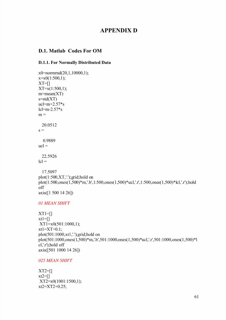
8/22/2019 Development of Univariate Control Chart for Non Normal Data
http://slidepdf.com/reader/full/development-of-univariate-control-chart-for-non-normal-data 73/87
61
APPENDIX D
D.1. Matlab Codes For OM
D.1.1. For Normally Distributed Data
x0=normrnd(20,1,10000,1);x=x0(1:500,1);
XT=[]XT=x(1:500,1);
m=mean(XT)
s=std(XT)ucl=m+2.57*s
lcl=m-2.57*sm =
20.0512s =
0.9889
ucl =
22.5926
lcl =
17.5097
plot(1:500,XT,'.');grid;hold on plot(1:500,ones(1,500)*m,'.b',1:500,ones(1,500)*ucl,'.r',1:500,ones(1,500)*lcl,'.r');hold
off
axis([1 500 14 26])
01 MEAN SHIFT
XT1=[]
xt1=[]
XT1=x0(501:1000,1);xt1=XT+0.1; plot(501:1000,xt1,'.');grid;hold on
plot(501:1000,ones(1,500)*m,'.b',501:1000,ones(1,500)*ucl,'.r',501:1000,ones(1,500)*l
cl,'.r');hold off axis([501 1000 14 26])
025 MEAN SHIFT
XT2=[]
xt2=[]
XT2=x0(1001:1500,1);xt2=XT2+0.25;
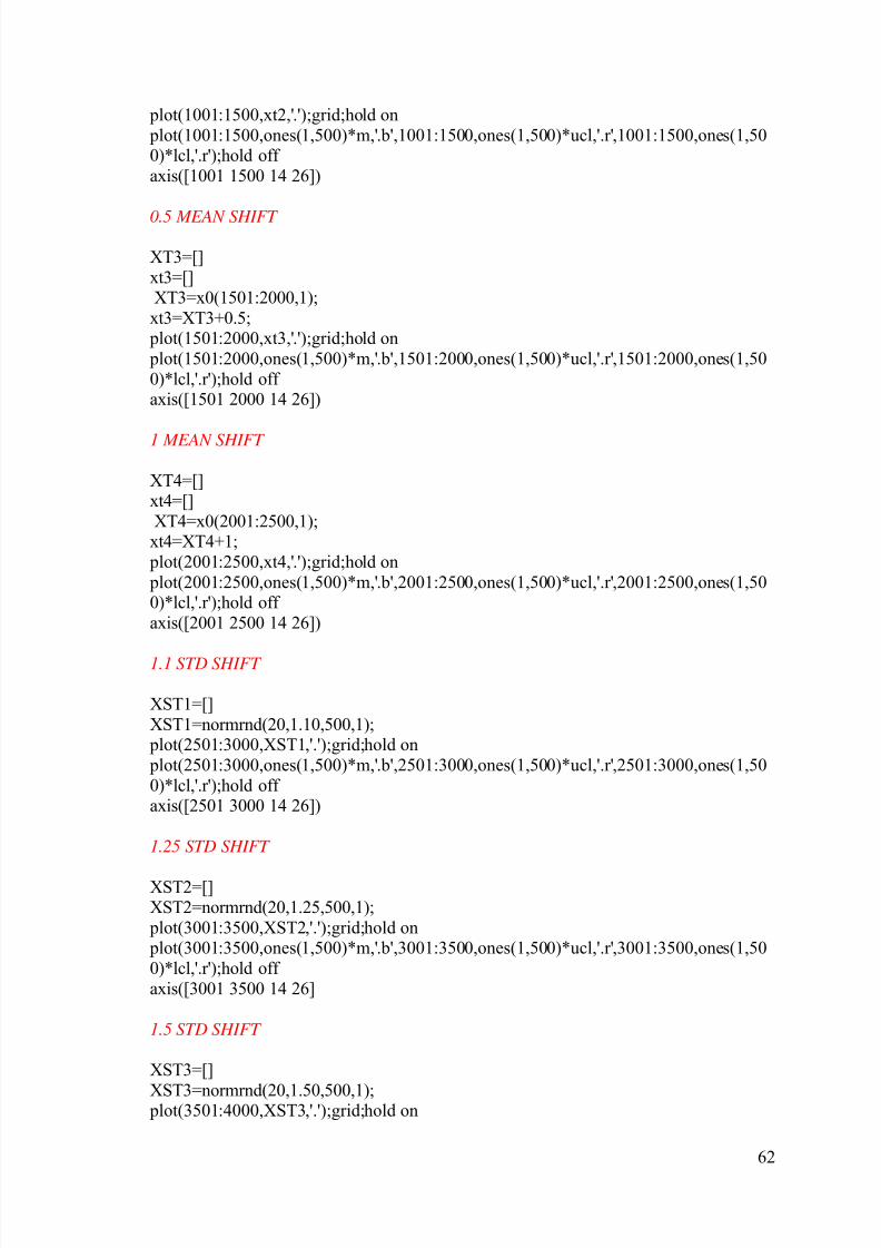
8/22/2019 Development of Univariate Control Chart for Non Normal Data
http://slidepdf.com/reader/full/development-of-univariate-control-chart-for-non-normal-data 74/87
62
plot(1001:1500,xt2,'.');grid;hold on
plot(1001:1500,ones(1,500)*m,'.b',1001:1500,ones(1,500)*ucl,'.r',1001:1500,ones(1,500)*lcl,'.r');hold off
axis([1001 1500 14 26])
0.5 MEAN SHIFT
XT3=[]
xt3=[]XT3=x0(1501:2000,1);
xt3=XT3+0.5; plot(1501:2000,xt3,'.');grid;hold on
plot(1501:2000,ones(1,500)*m,'.b',1501:2000,ones(1,500)*ucl,'.r',1501:2000,ones(1,50
0)*lcl,'.r');hold off axis([1501 2000 14 26])
1 MEAN SHIFT
XT4=[]xt4=[]
XT4=x0(2001:2500,1);xt4=XT4+1;
plot(2001:2500,xt4,'.');grid;hold on
plot(2001:2500,ones(1,500)*m,'.b',2001:2500,ones(1,500)*ucl,'.r',2001:2500,ones(1,500)*lcl,'.r');hold off
axis([2001 2500 14 26])
1.1 STD SHIFT
XST1=[]
XST1=normrnd(20,1.10,500,1); plot(2501:3000,XST1,'.');grid;hold on
plot(2501:3000,ones(1,500)*m,'.b',2501:3000,ones(1,500)*ucl,'.r',2501:3000,ones(1,50
0)*lcl,'.r');hold off axis([2501 3000 14 26])
1.25 STD SHIFT
XST2=[]XST2=normrnd(20,1.25,500,1);
plot(3001:3500,XST2,'.');grid;hold on plot(3001:3500,ones(1,500)*m,'.b',3001:3500,ones(1,500)*ucl,'.r',3001:3500,ones(1,50
0)*lcl,'.r');hold off
axis([3001 3500 14 26]
1.5 STD SHIFT
XST3=[]
XST3=normrnd(20,1.50,500,1); plot(3501:4000,XST3,'.');grid;hold on

8/22/2019 Development of Univariate Control Chart for Non Normal Data
http://slidepdf.com/reader/full/development-of-univariate-control-chart-for-non-normal-data 75/87
63
plot(3501:4000,ones(1,500)*m,'.b',3501:4000,ones(1,500)*ucl,'.r',3501:4000,ones(1,50
0)*lcl,'.r');hold off axis([3501 4000 14 26])
2 STD SHIFT
XST4=[]XST4=normrnd(20,2,500,1);
plot(4001:4500,XST4,'.');grid;hold on plot(4001:4500,ones(1,500)*m,'.b',4001:4500,ones(1,500)*ucl,'.r',4001:4500,ones(1,50
0)*lcl,'.r');hold off
BACK TO NORMAL OPERATION
XT5=[]
XT5=normrnd(20,1,500,1);
plot(4501:5000,XT5,'.');grid;hold on plot(4501:5000,ones(1,500)*m,'.b',4501:5000,ones(1,500)*ucl,'.r',4501:5000,ones(1,50
0)*lcl,'.r');hold off axis([4501 5000 14 26])
D.1.2. For Non-normally Distributed Data
x0=chi2rnd(5,10000,1);x=x0(1:1000,1);
XT=[]
XT=x(1:1000,1);m=mean(XT)
s=std(XT)ucl=m+2.57*s
lcl=m-2.57*s
m =4.8199
s =
2.9079ucl =
12.2931
lcl =
-2.6534 plot(1:1000,XT,'.');grid;hold on
plot(1:1000,ones(1,1000)*m,'.b',1:1000,ones(1,1000)*ucl,'.r',1:1000,ones(1,1000)*lcl,'.r
');hold off axis([1 1000 -10 30])

8/22/2019 Development of Univariate Control Chart for Non Normal Data
http://slidepdf.com/reader/full/development-of-univariate-control-chart-for-non-normal-data 76/87
64
01 MEAN SHIFT
XT1=[]
xt1=[]
XT1=x0(1001:1500,1);
xt1=XT(501:1000,1)+0.1; plot(1001:1500,xt1,'.');grid;hold on plot(1001:1500,ones(1,500)*m,'.b',1001:1500,ones(1,500)*ucl,'.r',1001:1500,ones(1,50
0)*lcl,'.r');hold off axis([1001 1500 -10 30])
025 MEAN SHIFT
XT2=[]xt2=[]
XT2=x0(1501:2000,1);
xt2=XT2+0.25; plot(1501:2000,xt2,'.');grid;hold on
plot(1501:2000,ones(1,500)*m,'.b',1501:2000,ones(1,500)*ucl,'.r',1501:2000,ones(1,500)*lcl,'.r');hold off
axis([1501 200 -10 30]
0.5 MEAN SHIFT
XT3=[]
xt3=[]XT3=x0(2001:2500,1);
xt3=XT3+0.5;
plot(2001:2500,xt3,'.');grid;hold on plot(2001:2500,ones(1,500)*m,'.b',2001:2500,ones(1,500)*ucl,'.r',2001:2500,ones(1,50
0)*lcl,'.r');hold off axis([2001 2500 -10 30])
1 MEAN SHIFT
XT4=[]xt4=[]
XT4=x0(2501:3000,1);xt4=XT4+1; plot(2501:3000,xt4,'.');grid;hold on
plot(2501:3000,ones(1,500)*m,'.b',2501:3000,ones(1,500)*ucl,'.r',2501:3000,ones(1,500)*lcl,'.r');hold off
axis([2501 3000 -10 30])
1.1 STD SHIFT
XST1=[]
XST1=normrnd(20,1.10,500,1);
plot(2501:3000,XST1,'.');grid;hold on
8/22/2019 Development of Univariate Control Chart for Non Normal Data
http://slidepdf.com/reader/full/development-of-univariate-control-chart-for-non-normal-data 77/87
65
plot(2501:3000,ones(1,500)*m,'.b',2501:3000,ones(1,500)*ucl,'.r',2501:3000,ones(1,50
0)*lcl,'.r');hold off axis([2501 3000 14 26])
1.25 STD SHIFT
XST2=[]XST2=normrnd(20,1.25,500,1);
plot(3001:3500,XST2,'.');grid;hold on plot(3001:3500,ones(1,500)*m,'.b',3001:3500,ones(1,500)*ucl,'.r',3001:3500,ones(1,50
0)*lcl,'.r');hold off axis([3001 3500 14 26])
1.5 STD SHIFT
XST3=[]
XST3=normrnd(20,1.50,500,1); plot(3501:4000,XST3,'.');grid;hold on
plot(3501:4000,ones(1,500)*m,'.b',3501:4000,ones(1,500)*ucl,'.r',3501:4000,ones(1,500)*lcl,'.r');hold off
axis([3501 4000 14 26])
2 STD SHIFT
XST4=[]
XST4=normrnd(20,2,500,1); plot(4001:4500,XST4,'.');grid;hold on
plot(4001:4500,ones(1,500)*m,'.b',4001:4500,ones(1,500)*ucl,'.r',4001:4500,ones(1,50
0)*lcl,'.r');hold off
BACK TO NORMAL OPERATION
XT5=[]
XT5=normrnd(20,1,500,1); plot(4501:5000,XT5,'.');grid;hold on
plot(4501:5000,ones(1,500)*m,'.b',4501:5000,ones(1,500)*ucl,'.r',4501:5000,ones(1,500)*lcl,'.r');hold off
axis([4501 5000 14 26])
D.1.3. For Industrial Data
XT=[]
XT=x(1:950,1);hist(XT)
normplot(XT)
m=mean(XT)s=std(XT)
ucl=m+2.57*slcl=m-2.57*s
8/22/2019 Development of Univariate Control Chart for Non Normal Data
http://slidepdf.com/reader/full/development-of-univariate-control-chart-for-non-normal-data 78/87
66
m =
0.4709
s =
0.1660ucl =
0.8975lcl =
0.0444
plot(1:950,XT,'.');grid;hold on
plot(1:950,ones(1,950)*m,'.b',1:950,ones(1,950)*ucl,'.r',1:950,ones(1,950)*lcl,'.r');holdoff
axis([1 950 -0.2 1.5])
XT1=[]
XT1=x(951:1179,1); plot(951:1179,XT1,'.');grid;hold on
plot(951:1179,ones(1,229)*m,'.b',951:1179,ones(1,229)*ucl,'.r',951:1179,ones(1,229)*lcl,'.r');hold off
axis([951 1179 -0.3 4])
D.2. Matlab Codes For NM
D.2.1. For Normally Distributed Data
x0=normrnd(20,1,10000,1);x=x0(1:1000,1);
[F2,xi2]=ksdensity(x,'npoints',5000,'width',0.075);
K2=[];for i=1:1000
[d,id]=min(abs(x(i)-xi2));
K2(i,1)=F2(id);end
y=normpdf(x,20,1); plot(x,y,'g.',xi2,F2,'b.');grid
>> E0=[];E0=y-K2;
m=mean(E0)
s=std(E0)ucl=m+2.57*s
lcl=m-2.57*sm =
-0.0107
s =
8/22/2019 Development of Univariate Control Chart for Non Normal Data
http://slidepdf.com/reader/full/development-of-univariate-control-chart-for-non-normal-data 79/87
67
0.0276ucl =
0.0603
lcl =
-0.0817figure(2);plot(1:1000,E0,'.');grid;hold on
>> figure(3);plot(1:1000,E0,'.');grid;hold on plot(ones(1,1000)*m,('.b'))
plot(ones(1,1000)*ucl,('.g')) plot(ones(1,1000)*lcl,('.g'))
axis([1 1000 -0.3 0.3])
01 MEAN SHIFT
XT=[]xt1=[]
XT=x0(1001:1500,1);xt1=XT+0.1;
ET=[];zt=[];
for j=1:500
zt=[x((j+500):1000);xt1(1:j)];[FZ,xiZ]=ksdensity(zt,'npoints',5000,'width',0.075);
Kt=[];for i=1:500
[d,id]=min(abs(zt(i)-xiZ));
Kt(i,1)=FZ(id);end
%yt=normpdf(zt(j),20,1);yt=normpdf(xt1(j),20,1);
ET(j,1)=yt-Kt(500);
endfigure(2);plot(1001:1500,ET,'.');grid;hold on
plot(1001:1500,ones(1,500)*m,'.b',1001:1500,ones(1,500)*ucl,'.r',1001:1500,ones(1,50
0)*lcl,'.r')
axis([1001 1500 -0.50 0.50])
025 MEAN SHIFT
XT1=[]
xt2=[]
XT1=x0(1501:2000,1);xt2=XT1+0.25;
ET1=[];
zt1=[];for j=1:500
zt1=[x((j+500):1000);xt2(1:j)];[FZ1,xiZ1]=ksdensity(zt1,'npoints',5000,'width',0.075);

8/22/2019 Development of Univariate Control Chart for Non Normal Data
http://slidepdf.com/reader/full/development-of-univariate-control-chart-for-non-normal-data 80/87
68
Kt1=[];
for i=1:500[d,id]=min(abs(zt1(i)-xiZ1));
Kt1(i,1)=FZ1(id);
end
%yt=normpdf(zt(j),20,1);yt1=normpdf(xt2(j),20,1);ET1(j,1)=yt1-Kt1(500);
endfigure(2);plot(1501:2000,ET1,'.');grid;hold on
plot(1501:2000,ones(1,500)*m,'.b',1501:2000,ones(1,500)*ucl,'.r',1501:2000,ones(1,500)*lcl,'.r')
axis([1501 2000 -0.50 0.50])
0.5 MEAN SHIFT
XT2=[]xt3=[]
XT2=x0(2001:2500,1);xt3=XT2+0.5;
ET2=[];zt2=[];
for j=1:500
zt2=[x((j+500):1000);xt3(1:j)];[FZ2,xiZ2]=ksdensity(zt2,'npoints',5000,'width',0.075);
Kt2=[];for i=1:500
[d,id]=min(abs(zt2(i)-xiZ2));
Kt2(i,1)=FZ2(id);end
%yt=normpdf(zt(j),20,1);yt2=normpdf(xt3(j),20,1);
ET2(j,1)=yt2-Kt2(500);
endfigure(2);plot(2001:2500,ET2,'.');grid;hold on
plot(2001:2500,ones(1,500)*m,'.b',2001:2500,ones(1,500)*ucl,'.r',2001:2500,ones(1,500)*lcl,'.r')
axis([2001 2500 -0.50 0.50])
1 MEAN SHIFT
XT3=[]
xt4=[]
XT3=x0(2501:3000,1);xt4=XT3+1;
ET3=[];
zt3=[];for j=1:500
zt3=[x((j+500):1000);xt4(1:j)];[FZ3,xiZ3]=ksdensity(zt3,'npoints',5000,'width',0.075);
8/22/2019 Development of Univariate Control Chart for Non Normal Data
http://slidepdf.com/reader/full/development-of-univariate-control-chart-for-non-normal-data 81/87
69
Kt3=[];
for i=1:500[d,id]=min(abs(zt3(i)-xiZ3));
Kt3(i,1)=FZ3(id);
end
%yt=normpdf(zt(j),20,1);yt3=normpdf(xt4(j),20,1);ET3(j,1)=yt3-Kt3(500);
endfigure(2);plot(2501:3000,ET3,'.');grid;hold on
plot(2501:3000,ones(1,500)*m,'.b',2501:3000,ones(1,500)*ucl,'.r',2501:3000,ones(1,500)*lcl,'.r')
axis([2501 3000 -0.50 0.50])
1.1 STD SHIFT
XT4=[]XT4=normrnd(20,1.1,500,1);
ET4=[];zt4=[];
for j=1:500zt4=[x((j+500):1000);XT4(1:j)];
[FZ4,xiZ4]=ksdensity(zt4,'npoints',5000,'width',0.075);
Kt4=[];for i=1:500
[d,id]=min(abs(zt4(i)-xiZ4));Kt4(i,1)=FZ4(id);
end
%yt=normpdf(zt(j),20,1);yt4=normpdf(XT4(j),20,1);
ET4(j,1)=yt4-Kt4(500);end
plot(3001:3500,ET4,'.');grid;hold on
figure(2);plot(3001:3500,ET4,'.');grid;hold on plot(3001:3500,ones(1,500)*m,'.b',3001:3500,ones(1,500)*ucl,'.r',3001:3500,ones(1,50
0)*lcl,'.r')
axis([3001 3500 -0.50 0.50])
1.25 STD SHIFT
XT5=[]XT5=normrnd(20,1.25,500,1);
ET5=[];
zt5=[];for j=1:500
zt5=[x((j+500):1000);XT5(1:j)];
[FZ5,xiZ5]=ksdensity(zt5,'npoints',5000,'width',0.075);Kt5=[];
for i=1:500
8/22/2019 Development of Univariate Control Chart for Non Normal Data
http://slidepdf.com/reader/full/development-of-univariate-control-chart-for-non-normal-data 82/87
70
[d,id]=min(abs(zt5(i)-xiZ5));
Kt5(i,1)=FZ5(id);end
%yt=normpdf(zt(j),20,1);
yt5=normpdf(XT5(j),20,1);
ET5(j,1)=yt5-Kt5(500);endfigure(2);plot(3501:4000,ET5,'.');grid;hold on
plot(3501:4000,ones(1,500)*m,'.b',3501:4000,ones(1,500)*ucl,'.r',3501:4000,ones(1,500)*lcl,'.r')
axis([3501 4000 -0.50 0.50])
1.5 STD SHIFT
XT6=[]
XT6=normrnd(20,1.5,500,1);
ET6=[];zt6=[];
for j=1:500zt6=[x((j+500):1000);XT6(1:j)];
[FZ6,xiZ6]=ksdensity(zt6,'npoints',5000,'width',0.075);Kt6=[];
for i=1:500
[d,id]=min(abs(zt6(i)-xiZ6));Kt6(i,1)=FZ6(id);
end%yt=normpdf(zt(j),20,1);
yt6=normpdf(XT6(j),20,1);
ET6(j,1)=yt6-Kt6(500);end
figure(2);plot(4001:4500,ET6,'.');grid;hold on plot(4001:4500,ones(1,500)*m,'.b',4001:4500,ones(1,500)*ucl,'.r',4001:4500,ones(1,50
0)*lcl,'.r')
axis([4001 4500 -0.50 0.50])
2 STD SHIFT
XT7=[]XT7=normrnd(20,2,500,1);ET7=[];
zt7=[];for j=1:500
zt7=[x((j+500):1000);XT7(1:j)];
[FZ7,xiZ7]=ksdensity(zt7,'npoints',5000,'width',0.075);Kt7=[];
for i=1:500
[d,id]=min(abs(zt7(i)-xiZ7));Kt7(i,1)=FZ7(id);
end%yt=normpdf(zt(j),20,1);
8/22/2019 Development of Univariate Control Chart for Non Normal Data
http://slidepdf.com/reader/full/development-of-univariate-control-chart-for-non-normal-data 83/87
71
yt7=normpdf(XT7(j),20,1);
ET7(j,1)=yt7-Kt7(500);end
figure(2);plot(4501:5000,ET7,'.');grid;hold on
plot(4501:5000,ones(1,500)*m,'.b',4501:5000,ones(1,500)*ucl,'.r',4501:5000,ones(1,50
0)*lcl,'.r')axis([4501 5000 -0.50 0.50])
BACK TO NORMAL OPERATION
X8=[]X8=normrnd(20,1,1000,1);
E8=[];
[F8,xi8]=ksdensity(X8,'npoints',5000,'width',0.075);K8=[];
for i=1:1000
[d,id]=min(abs(X8(i)-xi8));K8(i,1)=F8(id);
endy8=normpdf(X8,20,1);
plot(X8,y8,'g.',xi8,F8,'b.');grid>> E8=[];
E8=y8-K8;
figure(2);plot(5001:6000,E8,'.');grid;hold on plot(5001:6000,ones(1,1000)*m,'.b',5001:6000,ones(1,1000)*ucl,'.r',5001:6000,ones(1,
1000)*lcl,'.r')axis([5001 6000 -0.30 0.30])
D.2.2. For Non-normally Distributed Data
x0=chi2rnd(5,10000,1);
x=x0(1:1000,1),[F2,xi2]=ksdensity(x,'npoints',5000,'width',0.075);
K2=[];for i=1:1000
[d,id]=min(abs(x(i)-xi2));K2(i,1)=F2(id);end
y=chi2pdf(x,5); plot(x,y,'g.',xi2,F2,'b.');grid
E0=[];
E0=y-K2;figure(2);plot(1:1000,E0,'.');grid;hold on
>> figure(3);plot(1:1000,E0,'.');grid;hold on
m=mean(E0)s=std(E0)
ucl=m+2.57*slcl=m-2.57*s

8/22/2019 Development of Univariate Control Chart for Non Normal Data
http://slidepdf.com/reader/full/development-of-univariate-control-chart-for-non-normal-data 84/87
72
plot(ones(1,1000)*m,('.b'))
plot(ones(1,1000)*ucl,('.g')) plot(ones(1,1000)*lcl,('.g'))
axis([1 1000 -0.1 0.1])
m =
-0.0064s =
0.0169
ucl =
0.0370
lcl =
-0.0499
01 MEAN SHIFT
XT=[]
xt1=[]XT=x0(1001:1500,1);
xt1=XT+0.1;
ET=[];zt=[];
for j=1:500zt=[x((j+500):1000);xt1(1:j)];
[FZ,xiZ]=ksdensity(zt,'npoints',5000,'width',0.075);
Kt=[];for i=1:500
[d,id]=min(abs(zt(i)-xiZ));Kt(i,1)=FZ(id);
end
%yt=chi2pdf(zt(j),10);yt=chi2pdf(xt1(j),5);
ET(j,1)=yt-Kt(500);end
plot(1001:1500,ET,'.');grid;hold on plot(1001:1500,ones(1,500)*m,'.b',1001:1500,ones(1,500)*ucl,'.r',1001:1500,ones(1,500)*lcl,'.r')
axis([1001 1500 -0.3 0.3])
025 MEAN SHIFT
XT1=[]
xt2=[]
XT1=x0(1501:2000,1);xt2=XT1+0.25;
ET1=[];zt1=[];

8/22/2019 Development of Univariate Control Chart for Non Normal Data
http://slidepdf.com/reader/full/development-of-univariate-control-chart-for-non-normal-data 85/87
73
for j=1:500
zt1=[x((j+500):1000);xt2(1:j)];[FZ1,xiZ1]=ksdensity(zt1,'npoints',5000,'width',0.075);
Kt1=[];
for i=1:500
[d,id]=min(abs(zt1(i)-xiZ1));Kt1(i,1)=FZ1(id);end
%yt=chi2pdf(zt(j),10);yt1=chi2pdf(xt2(j),5);
ET1(j,1)=yt1-Kt1(500);end
plot(1501:2000,ET1,'.');grid;hold on
plot(1501:2000,ones(1,500)*m,'.b',1501:2000,ones(1,500)*ucl,'.r',1501:2000,ones(1,500)*lcl,'.r')
axis([1501 2000 -0.3 0.3])
0.5 MEAN SHIFT
XT2=[]
xt3=[]XT2=x0(2001:2500,1);
xt3=XT2+0.5;
ET2=[];zt2=[];
for j=1:500zt2=[x((j+500):1000);xt3(1:j)];
[FZ2,xiZ2]=ksdensity(zt2,'npoints',5000,'width',0.075);
Kt2=[];for i=1:500
[d,id]=min(abs(zt2(i)-xiZ2));Kt2(i,1)=FZ2(id);
end
%yt=chi2pdf(zt(j),10);yt2=chi2pdf(xt3(j),5);
ET2(j,1)=yt2-Kt2(500);end
plot(2001:2500,ET2,'.');grid;hold on plot(2001:2500,ones(1,500)*m,'.b',2001:2500,ones(1,500)*ucl,'.r',2001:2500,ones(1,500)*lcl,'.r')
axis([2001 2500 -0.3 0.3])
1 MEAN SHIFT
XT3=[]
xt4=[]
XT3=x0(2501:3000,1);xt4=XT3+1;
ET3=[];zt3=[];

8/22/2019 Development of Univariate Control Chart for Non Normal Data
http://slidepdf.com/reader/full/development-of-univariate-control-chart-for-non-normal-data 86/87
74
for j=1:500
zt3=[x((j+500):1000);xt4(1:j)];[FZ3,xiZ3]=ksdensity(zt3,'npoints',5000,'width',0.075);
Kt3=[];
for i=1:500
[d,id]=min(abs(zt3(i)-xiZ3));Kt3(i,1)=FZ3(id);end
%yt=normpdf(zt(j),20,1);yt3=chi2pdf(xt4(j),5);
ET3(j,1)=yt3-Kt3(500);end
plot(2501:3000,ET3,'.');grid;hold on
figure(2);plot(2501:3000,ET3,'.');grid;hold on plot(2501:3000,ones(1,500)*m,'.b',2501:3000,ones(1,500)*ucl,'.r',2501:3000,ones(1,50
0)*lcl,'.r')
axis([2501 3000 -0.3 0.3])
BACK TO NORMAL OPERATION
x0=chi2rnd(5,10000,1);xS=x0(3001:4000,1),
[FS,xiS]=ksdensity(xS,'npoints',5000,'width',0.075);
KS=[];for i=1:1000
[d,id]=min(abs(xS(i)-xiS));KS(i,1)=FS(id);
end
yS=chi2pdf(xS,5); plot(xS,yS,'g.',xiS,FS,'b.');grid
ES=[];ES=yS-KS;
m=mean(ES)
s=std(ES)ucl=m+2.57*s
lcl=m-2.57*s plot(3001:4000,ES,'.');grid;hold on
plot(3001:4000,ones(1,1000)*m,'.b',3001:4000,ones(1,1000)*ucl,'.r',3001:4000,ones(1,1000)*lcl,'.r')axis([3001 4000 -0.1 0.1])
D.2.3. For Industrial Data
xt=x(1:950);
normplot(xt)[F2,xi2]=ksdensity(xt,'npoints',5000,'width',0.05,'kernel','normal');
figure(1);y2=normpdf(xt,0.4741,0.1674); plot(xi2,F2,'b.',xt,y2,'g.');grid

8/22/2019 Development of Univariate Control Chart for Non Normal Data
http://slidepdf.com/reader/full/development-of-univariate-control-chart-for-non-normal-data 87/87
K2=[];for i=1:950
[d,id]=min(abs(xt(i)-xi2));
K2(i,1)=F2(id);
endE0=[];E0=y2-K2;
m=mean(E0)s=std(E0)
ucl=m+2.57*slcl=m-2.57*s
m =
-0.0674s =
0.2198ucl =
0.4976
lcl =
-0.6324
figure(3);plot(1:950,E0,'.');grid;hold on plot(ones(1,950)*m,('.b'))
plot(ones(1,950)*ucl,('.g')) plot(ones(1,950)*lcl,('.g'))
XT=[]XT=x(950:1179,1);
ET=[];
zt=[];for j=1:230
zt=[x((j+1):230);XT(1:j)];[FZ,xiZ]=ksdensity(zt,'npoints',5000,'width',0.05,'kernel','normal');
Kt=[];
for i=1:230
[d,id]=min(abs(zt(i)-xiZ));Kt(i,1)=FZ(id);end