development of tumor microenvironment-oriented digital
TRANSCRIPT

DOI numeris (suteikiamas atsiuntus disertaciją spausdinti)
https://orcid.org/0000-0001-2345-6789
VILNIUS UNIVERSITY
Mindaugas
MORKŪNAS
Development of Tumor
Microenvironment-Oriented Digital
Pathology Methods for Whole Slide
Image Segmentation and Classification
DOCTORAL DISSERTATION
Technological Sciences
Informatics Engineering T 007
VILNIUS 2021

This dissertation was written between 2016 and 2020 at Vilnius University.
Academic supervisor:
Assoc. Prof. Dr. Povilas Treigys (Vilnius University, Technological
Sciences, Informatics Engineering – T 007).
Academic consultant:
Prof. Dr. Arvydas Laurinavičius (Vilnius University, Medicine and Health
Sciences, Medicine – M 001).

3
DOI numeris (suteikiamas atsiuntus disertaciją spausdinti)
https://orcid.org/0000-0001-2345-6789
VILNIAUS UNIVERSITETAS
Mindaugas
MORKŪNAS
Naviko Mikroaplinkai Pritaikytų Pilno
Kadro Vaizdo Segmentavimo ir
Klasifikavimo Skaitmeninės Patologijos
Metodų Kūrimas
DAKTARO DISERTACIJA
Technologijos mokslai
Informatikos inžinerija T 007
VILNIUS 2021
Disertacija rengta 2016–2020 metais Vilniaus universitete.
Mokslinis vadovas:
doc. dr. Povilas Treigys (Vilniaus universitetas, technologijos mokslai,
informatikos inžinerija – T 007).
Mokslinis konsultantas:
prof. dr. Arvydas Laurinavičius (Vilniaus universitetas, medicinos ir
sveikatos mokslai, medicina – M 001).

ABSTRACT
To better serve cancer patients, diagnostic and digital pathology methods
focus on more novel targets. One of such targets is the tumor
microenvironment. The increasing significance of the tumor
microenvironment in cancer biology has caused a major shift of cancer
treatment and research from a tumor-centric model to a tumor
microenvironment-centric one. However, machine vision-dependent digital
pathology methods are still very tumor cell-centric and largely ignore the
tumor microenvironment. This work has set the aim to investigate and
propose new histopathology image segmentation and classification methods
by targeting tumor microenvironment-related histologic tissue components.
Firstly, convolutional neural networks were identified as a group of state-of-
the-art methods of sufficient capacity to handle multiple histologic object
segmentation. Then, the existing tumor cell segmentation method was
adapted and extended for lymphocyte segmentation and identification. Next,
fibrous collagen was identified as a novel tumor microenvironment-borne
target for segmentation in bright-field images of tumorous tissue. To address
the collagen fiber segmentation task, a fully convolutional neural network-
based approach was developed. Finally, an approach integrating knowledge
gained in previous experiments was proposed enabling segmentation of
lymphocytes, tumor cell nuclei, stromal cell nuclei, collagen fibers, and
major tissue compartments. Additionally, by the engineering of image
features, a whole slide image transformation was introduced, enabling the
prediction of therapeutic biomarker status for individual breast cancer
patients from complete tumor tissue whole-slide images. Proposed methods
were extensively tested in an experimental setup on private in-house
annotated histologic image datasets and public datasets and a competition
challenge. The proposed methods were comparable to the state-of-the-art
methods while at the same time providing special additional features.
6
SANTRAUKA
Siekiant didesnės naudos onkologiniams pacientams sukurti diagnostiniai
ir skaitmeniniai patologijos metodai, daug dėmesio skiriantys naujiems
tyrimo taikiniams. Vienas iš tokių taikinių yra naviko mikroaplinka.
Ryškėjanti naviko mikroaplinkos svarba vėžio biologijoje lemia akivaizdų
vėžio gydymo ir tyrimų posūkį nuo naviko ląstelėms pritaikyto link naviko
mikroaplinkai pritaikyto modelio. Tačiau nuo kompiuterinės regos
priklausomi skaitmeninės patologijos metodai vis dar yra stipriai orientuoti į
naviko ląsteles ir iš esmės ignoruoja naviko mikroaplinką. Šiame darbe
užsibrėžtas tikslas ištirti ir pasiūlyti naujus histopatologijos vaizdo
segmentavimo ir klasifikavimo metodus, skirtus su naviko mikroaplinka
susijusiems histologiniams audinių komponentams. Pirma, konvoliuciniai
neuroniniai tinklai identifikuoti kaip pažangiausių metodų, pakankamai
pajėgių daugeliui histologinių objektų segmentuoti, grupė. Tada limfocitams
segmentuoti ir identifikuoti pritaikytas ir išplėstas esamas naviko ląstelių
segmentavimo metodas. Toliau skaidulinis kolagenas identifikuotas kaip
naujas iš naviko mikroaplinkos atsirandantis taikinys, kurį galima
segmentuoti naviko audinių šviesinės mikroskopijos vaizduose. Kolageno
skaidulų segmentavimo užduočiai spręsti sukurtas visiškai konvoliucinis
neuroninių tinklų metodas. Galiausiai pasiūlytas integruotas metodas,
sujungiantis ankstesniuose eksperimentuose įgytas žinias ir leidžiantis
segmentuoti limfocitų, naviko ląstelių, stromos ląstelių branduolius,
kolageno skaidulas ir pagrindinius audinių tipus. Be to, vaizdo požymių
inžinerijos būdu įvestas patologijos pilno kadro vaizdo transformavimas,
pritaikytas nuspėti krūties vėžiu sergančių pacientų terapinio biožymens
būseną. Siūlomi metodai išbandyti eksperimentais, naudojant tiek privačius,
tiek viešus anotuotų histologinių vaizdų duomenų rinkinius bei tarptautinio
iššūkio varžybose. Siūlomi metodai buvo sulyginami su susijusiais
pažangiausiais metodais, tuo pat metu suteikdami papildomų specialių
funkcionalumų.
7
List of Abbreviations
AE Autoencoder
ANN Artificial Neural Network
AUC
Area Under the Receiver Operating Characteristic
Curve
CNN Convolutional Neural Networks
CSM Collagen Segmentation Map
DL Deep Learning
ECM Extracellular Matrix
FA Factor Analysis
FCNN Fully Convolutional Neural Networks
GT Ground Truth
H&E Hematoxylin and Eosin
HOG Histogram of Oriented Gradients
IM Invasive Margin
IoU Intersection Over Union
MIL Multiple Instance Learning
ML Machine Learning
MLP Multilayer Perceptron
nits Number of Iterations
RDF Random Decision Forest
ROC Receiver Operating Characteristic
SHG Second Harmonic Generation
SVM Support-Vector Machine
TCGA The Cancer Genome Atlas
TMA Tissue Microarray
TME Tumor Microenvironment
WSI Whole Slide Image
8
Glossary of Biomedical Terms
Histology Histology is the study of the microscopic anatomy of
body tissues.
Histopathology Histopathology is the branch of histology that includes
the microscopic identification and study of diseased
tissue.
H&E Hematoxylin and Eosin staining is a technique to stain
otherwise transparent tissue sections. It is the most widely
used staining in medical diagnosis - H&E is applied to
almost every sample of tissue being assessed by a medical
pathologist.
IHC Immunohistochemistry (immunostaining, IHC) is a
special tissue staining technique requiring special
machinery and skilled technicians. The technique
leverages the interaction of antibody and antigen (hence
the “immuno-”). IHC tests are very specific and can
inform where exactly an assay target is located in the
tissue.
ECM The extracellular matrix is the material filling space in
between cells. ECM is critical for human physiology by
providing such functions as passive structural support,
cell mobility regulation by adhesion, cell-to-cell signaling
mediation, mechanical-to-molecular signal conversion,
material storage.
Collagen Collagen is the most abundant protein in the human body.
It is a major structural component of the extracellular
matrix. Collagen molecules form fibers that interconnect
to form a supportive environment for growing cells and
tissues. Within the tumor microenvironment, specifically
aligned collagen has been shown to stimulate tumor
progression by directing the migration of metastatic cells
along its structural framework.
Stroma Stroma is a tissue type providing a structural or
connective function and protects other functional tissues.
Stroma is made of stromal cells and largely ECM.
9
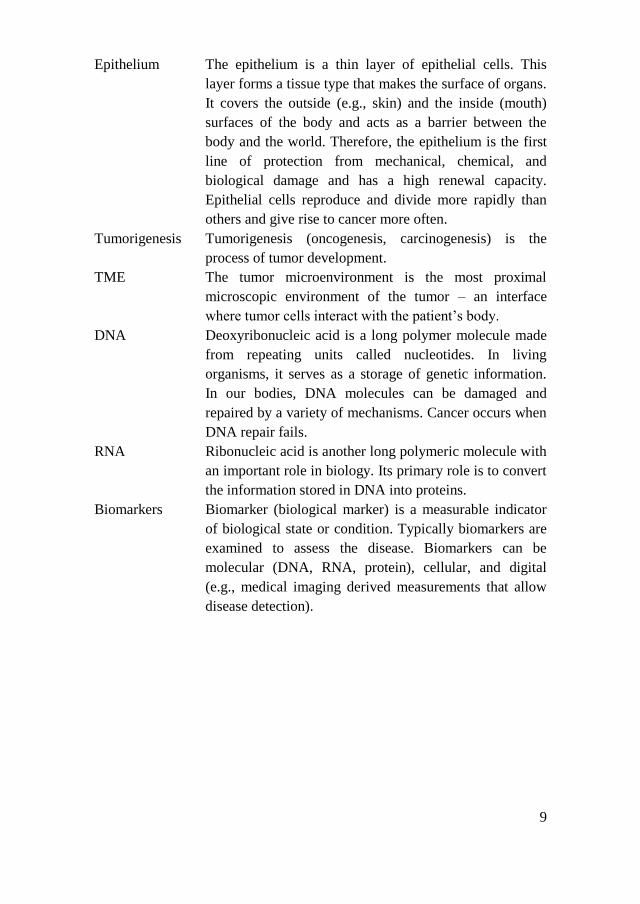
Epithelium The epithelium is a thin layer of epithelial cells. This
layer forms a tissue type that makes the surface of organs.
It covers the outside (e.g., skin) and the inside (mouth)
surfaces of the body and acts as a barrier between the
body and the world. Therefore, the epithelium is the first
line of protection from mechanical, chemical, and
biological damage and has a high renewal capacity.
Epithelial cells reproduce and divide more rapidly than
others and give rise to cancer more often.
Tumorigenesis Tumorigenesis (oncogenesis, carcinogenesis) is the
process of tumor development.
TME The tumor microenvironment is the most proximal
microscopic environment of the tumor – an interface
where tumor cells interact with the patient’s body.
DNA Deoxyribonucleic acid is a long polymer molecule made
from repeating units called nucleotides. In living
organisms, it serves as a storage of genetic information.
In our bodies, DNA molecules can be damaged and
repaired by a variety of mechanisms. Cancer occurs when
DNA repair fails.
RNA Ribonucleic acid is another long polymeric molecule with
an important role in biology. Its primary role is to convert
the information stored in DNA into proteins.
Biomarkers Biomarker (biological marker) is a measurable indicator
of biological state or condition. Typically biomarkers are
examined to assess the disease. Biomarkers can be
molecular (DNA, RNA, protein), cellular, and digital
(e.g., medical imaging derived measurements that allow
disease detection).

TABLE OF CONTENTS
1. INTRODUCTION..................................................................................... 12
1.1. Research Context ............................................................................... 12
1.2. Relevance of the Research ................................................................. 15
1.3. Object of the Dissertation ................................................................... 17
1.4. Aim and Tasks of the Dissertation ..................................................... 17
1.5. Bioethics ............................................................................................. 17
1.6. Scientific Novelty of the Research ..................................................... 18
1.7. Defended Statements .......................................................................... 19
1.8. Approbation of Research .................................................................... 19
2. LITERATURE REVIEW OF DIGITAL IMAGE ANALYSIS
METHODS IN PATHOLOGY ............................................................................. 22
2.1. Cancer Biology, Tumor Evolution, and the Tumor Microenvironment ... 22
2.2. Machine Vision for Digital Pathology ............................................... 24
2.2.1. Digital Pathology Grading Systems .......................................... 26
2.2.2. Tumor Cell-Oriented Computational Techniques ..................... 29
2.2.3. TME-Oriented Computational Techniques ................................ 35
2.2.4. Ground Truth for Digital Pathology ......................................... 39
2.2.5. Tumor Compartment-Agnostic Techniques .................................... 40
2.3. Related Research in Lithuania ............................................................ 41
2.4. Chapter Conclusions .......................................................................... 42
3. ANALYSIS OF ML METHODS FOR EPITHELIUM-STROMA
CLASSIFICATION ............................................................................................... 43
3.1. Experiment Design ............................................................................. 43
3.1.1. Datasets ..................................................................................... 44
3.1.2. Superpixel Descriptors .............................................................. 47
3.1.3. Machine Learning Models ......................................................... 48
3.2. Results ................................................................................................ 52
3.3. Chapter Conclusions .......................................................................... 56
4. METHOD FOR CELL NUCLEI SEGMENTATION WITH
LYMPHOCYTE IDENTIFICATION .................................................................. 57
4.1. Experiment Design ............................................................................. 57
4.1.1. Datasets ..................................................................................... 59
4.1.2. Cell Nuclei Segmentation Models .............................................. 62
4.1.3. Cell Nuclei Classifiers ............................................................... 64
4.2. Results ................................................................................................ 64
4.2.1. Nuclei Segmentation .................................................................. 65
4.2.2. Nuclei Classification ................................................................. 67
4.2.3. Workflow Evaluation ................................................................. 69
4.3. Chapter Conclusions .......................................................................... 72
11
5. COLLAGEN FRAMEWORK SEGMENTATION ............................... 74
5.1. Experiment Design ............................................................................. 74
5.1.1. Datasets ..................................................................................... 75
5.1.2. Generation of Ground Truth Masks .......................................... 77
5.1.3. Modified U-Net Model for Collagen Segmentation ................... 78
5.1.4. Collagen Fiber Morphometry .................................................... 82
5.2. Results ................................................................................................ 85
5.3. Chapter Conclusions .......................................................................... 95
6. MULTIPLE CLASS HISTOPATHOLOGY OBJECT
SEGMENTATION FOR TUMOR CLASSIFICATION .................................... 97
6.1. Experiment Design ............................................................................. 97
6.1.1. Dataset ...................................................................................... 98
6.1.2. U-Net Segmentation Model ..................................................... 101
6.1.3. Tissue Morphometry ................................................................ 102
6.1.4. WSI Classification ................................................................... 104
6.2. Results .............................................................................................. 106
6.2.1. WSI Segmentation .................................................................... 106
6.2.2. WSI Classification ................................................................... 108
6.2.3. Evaluation ............................................................................... 108
6.3. Chapter Conclusions ........................................................................ 110
GENERAL CONCLUSIONS ........................................................................ 111
REFERENCES ............................................................................................... 114

12
1. INTRODUCTION
1.1. Research Context
As humanity dwells in the age of data, a considerable part of our daily
activities is captured digitally and gets analyzed. A vast amount of digital
information is acquired in a clinical setting as image data using well-
established medical imaging techniques such as X-ray, magnetic resonance
imaging (MRI), computed tomography (CT), ultrasound, and many more.
Digital image analysis (DIA) is used to extract meaningful information
contained in images. When applied to medical images, DIA informs
treatment decisions and directly affects patients’ lives. Therefore, DIA
algorithms particularly those based on machine learning (ML) whose use is
intended for specific medical purposes qualify as medical or diagnostic
devices and have to undergo regulatory clearances. There are hundreds of
DIA-based medical devices cleared for clinical use worldwide for automated
labeling, visualization, and quantification of organ (brain, lung, breast,
prostate, cardiovascular system, thyroid) structures, documentation of
abnormalities, tumor contouring for therapy planning from CT scans, X-ray
or MR images, retinal diseases diagnosis from ophthalmic images, assistance
in the analysis of ultrasound images.
In this context, cancer diagnoses often rely on analyzing visual
information contained in the microscopic anatomy (histology) of surgically
removed tumor tissues. In a standard diagnostic workup, laboratory-
processed tissue specimens are placed on glass slides and routinely stained
with hematoxylin and eosin (H&E) stains to color otherwise transparent
tissue sections [1]. Alternative staining techniques are available and
commonly are referred to as “special stains”. Stained slides are presented for
patologist manual review under an optical microscope (see Fig. 1.1).
Differential diagnosis of tumors aims to classify a malignancy into clinically
relevant categories. Hence, a pathology diagnosis implies a label that is
applied to a patient and enables further decisions about treatment and
prognosis in the context of other clinical information. To arrive at a
diagnosis, pathologists must consider many biological factors of pathology,
usually presented as manual or digital assessment endpoints such as
qualitative or quantitative evaluation of the size and shape, density, and
alignment of tumorous tissue components. Objective, accurate, and
standardized phenotyping of microscopic manifestations of the disease
(histopathology) is a convenient system to guide treatment decisions.
13
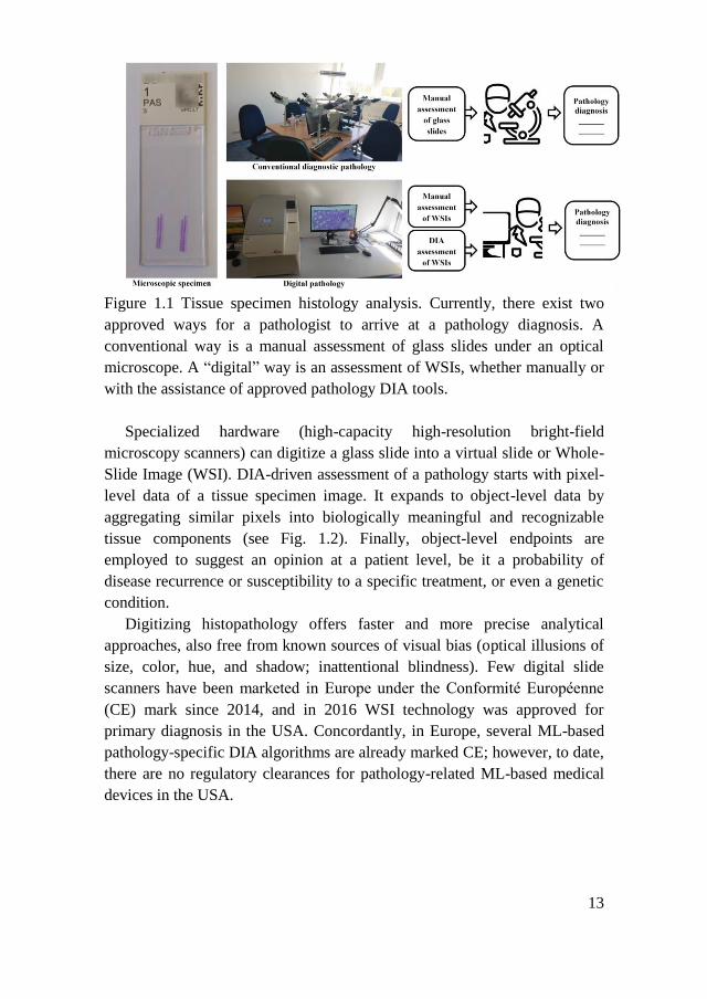
Figure 1.1 Tissue specimen histology analysis. Currently, there exist two
approved ways for a pathologist to arrive at a pathology diagnosis. A
conventional way is a manual assessment of glass slides under an optical
microscope. A “digital” way is an assessment of WSIs, whether manually or
with the assistance of approved pathology DIA tools.
Specialized hardware (high-capacity high-resolution bright-field
microscopy scanners) can digitize a glass slide into a virtual slide or Whole-
Slide Image (WSI). DIA-driven assessment of a pathology starts with pixel-
level data of a tissue specimen image. It expands to object-level data by
aggregating similar pixels into biologically meaningful and recognizable
tissue components (see Fig. 1.2). Finally, object-level endpoints are
employed to suggest an opinion at a patient level, be it a probability of
disease recurrence or susceptibility to a specific treatment, or even a genetic
condition.
Digitizing histopathology offers faster and more precise analytical
approaches, also free from known sources of visual bias (optical illusions of
size, color, hue, and shadow; inattentional blindness). Few digital slide
scanners have been marketed in Europe under the Conformité Européenne
(CE) mark since 2014, and in 2016 WSI technology was approved for
primary diagnosis in the USA. Concordantly, in Europe, several ML-based
pathology-specific DIA algorithms are already marked CE; however, to date,
there are no regulatory clearances for pathology-related ML-based medical
devices in the USA.
14
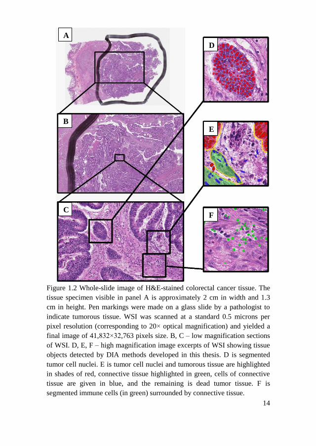
Figure 1.2 Whole-slide image of H&E-stained colorectal cancer tissue. The
tissue specimen visible in panel A is approximately 2 cm in width and 1.3
cm in height. Pen markings were made on a glass slide by a pathologist to
indicate tumorous tissue. WSI was scanned at a standard 0.5 microns per
pixel resolution (corresponding to 20× optical magnification) and yielded a
final image of 41,832×32,763 pixels size. B, C – low magnification sections
of WSI. D, E, F – high magnification image excerpts of WSI showing tissue
objects detected by DIA methods developed in this thesis. D is segmented
tumor cell nuclei. E is tumor cell nuclei and tumorous tissue are highlighted
in shades of red, connective tissue highlighted in green, cells of connective
tissue are given in blue, and the remaining is dead tumor tissue. F is
segmented immune cells (in green) surrounded by connective tissue.
A
B
C F
E
D

15
1.2. Relevance of the Research
Advanced comprehensive analysis of solid tumors brings benefits to
cancer patients. Tumor profiling by DNA, RNA, and protein biomarkers
leads towards personalized curative decisions in oncology [2]. Targeted
medications are proving invaluable for precisely pre-selected groups of
patients. Therefore, medical pathologists use well-established methods to
analyze solid tumor histology under an optical microscope to define groups
of susceptible patients.
For a long time, diagnostic pathology was mainly focused on tumor cells.
Tumor cell genetics explains many aspects of cancer development, but a
growing tumor progresses while closely interacting with the patient’s body
(host). The tumor microenvironment (TME) can be understood as an
interface of this interaction (the most proximal microscopic environment of
the tumor) together with the host-allied interacting counterparts – cells of the
inner and outer surface of organs and blood vessels, cells of connective,
muscle, fatty, and neural tissues, cells of immune origin, and the material
filling space in between cells (extracellular matrix (ECM)). Aggressive
tumors exploit these interactions to benefit their growth by ensuring the
supply of oxygen and nutrients, creating favorable conditions for the
movement and spread of metastatic cells. TME has become a special topic in
oncology due to our growing understanding of its function and role in tumor
development. It is undisputed that TME assessment can provide critical
therapeutic information [3-5], especially when dealing with tumors with
ambiguous histology. Recent research reveals TME as an emerging target for
personalized anti-cancer therapy [6-9].
In fact, digital pathology is even more tumor cell-centric than diagnostic
pathology and largely ignores the TME. A plethora of DIA methods is
available for tumor cell detection, segmentation, and classification.
Nevertheless, methods targeting TME cells are being researched. For
example, tumor-infiltrating immune cells (particularly lymphocytes) are
important TME-born targets that can efficiently be detected, counted, and
their density in tissue can be estimated by existing DIA methods [10-13].
However, lymphocyte segmentation is merely mentioned in a few research
papers. Similarly, connective tissue cells (stromal cells) are often mentioned
in the context of cell segmentation problems not as a primary target but
rather as hard-to-recognize cells negatively impacting the segmentation of
tumor cells [14, 15]. Therefore, DIA methods specifically targeting TME-
born cell types need to be developed.
16
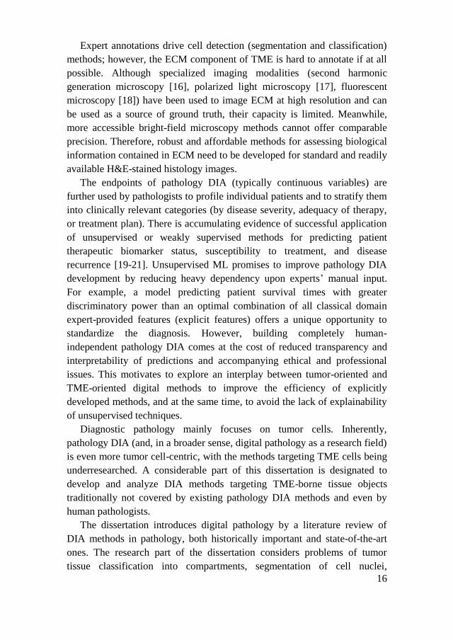
Expert annotations drive cell detection (segmentation and classification)
methods; however, the ECM component of TME is hard to annotate if at all
possible. Although specialized imaging modalities (second harmonic
generation microscopy [16], polarized light microscopy [17], fluorescent
microscopy [18]) have been used to image ECM at high resolution and can
be used as a source of ground truth, their capacity is limited. Meanwhile,
more accessible bright-field microscopy methods cannot offer comparable
precision. Therefore, robust and affordable methods for assessing biological
information contained in ECM need to be developed for standard and readily
available H&E-stained histology images.
The endpoints of pathology DIA (typically continuous variables) are
further used by pathologists to profile individual patients and to stratify them
into clinically relevant categories (by disease severity, adequacy of therapy,
or treatment plan). There is accumulating evidence of successful application
of unsupervised or weakly supervised methods for predicting patient
therapeutic biomarker status, susceptibility to treatment, and disease
recurrence [19-21]. Unsupervised ML promises to improve pathology DIA
development by reducing heavy dependency upon experts’ manual input.
For example, a model predicting patient survival times with greater
discriminatory power than an optimal combination of all classical domain
expert-provided features (explicit features) offers a unique opportunity to
standardize the diagnosis. However, building completely human-
independent pathology DIA comes at the cost of reduced transparency and
interpretability of predictions and accompanying ethical and professional
issues. This motivates to explore an interplay between tumor-oriented and
TME-oriented digital methods to improve the efficiency of explicitly
developed methods, and at the same time, to avoid the lack of explainability
of unsupervised techniques.
Diagnostic pathology mainly focuses on tumor cells. Inherently,
pathology DIA (and, in a broader sense, digital pathology as a research field)
is even more tumor cell-centric, with the methods targeting TME cells being
underresearched. A considerable part of this dissertation is designated to
develop and analyze DIA methods targeting TME-borne tissue objects
traditionally not covered by existing pathology DIA methods and even by
human pathologists.
The dissertation introduces digital pathology by a literature review of
DIA methods in pathology, both historically important and state-of-the-art
ones. The research part of the dissertation considers problems of tumor
tissue classification into compartments, segmentation of cell nuclei,
17
classification of segmented nuclei, segmentation of tissue collagen carcass,
and feature space engineering to detect tissue characteristics indicative of
pathologic condition.
1.3. Object of the Dissertation
The object of this dissertation is tumor microenvironment compartment
analysis in the whole-slide routinely stained histopathological images.
1.4. Aim and Tasks of the Dissertation
The aim of this dissertation is to investigate and propose new
histopathology image segmentation and classification methods by targeting
tumor microenvironment-related histologic tissue components.
With the view of realizing this aim, the following research tasks must be
completed:
1. Develop and evaluate a colorectal tumor epithelium-stroma
compartment classification method.
2. Propose a lightweight state-of-the-art tumor cell nuclei segmentation
and classification method for the analysis of the microenvironment
of breast and colorectal tumors.
3. Inspect existing collagen framework analysis methods and network
features and develop a method to capture fibrous tumor
microenvironment collagen framework in bright-field
histopathological microscopy images and investigate whether
obtained framework quantitative features can be used to predict
differences in survival between different groups of breast cancer
patients.
4. Develop and generalize a deep convolutional neural network method
enabling simultaneous segmentation and classification of tumor
microenvironment tissue compartments of the varying input WSI
sizes for breast cancer patient therapeutic biomarker status
classification.
1.5. Bioethics
The results obtained in Chapter 5 involved analysis of patient follow-up
data, therefore the Lithuanian Bioethics Committee approved this study

18
(reference number: 40, date 2007-04-26, updated 2017-09-12). Other studies
did not require bioethics approval.
1.6. Scientific Novelty of the Research
1. It was experimentally demonstrated that a convolutional neural network
(CNN) based model trained directly on image data classifies colorectal
tumor tissue more accurately than a support vector machine (SVM),
random forest classifier (RDF), or multilayer perceptron (MLP) models
trained on color and texture features of the same images.
2. Extensive research provides unequivocal evidence of fully convolutional
neural networks (FCNN) being a state-of-the-art method for cell nuclei
segmentation tasks. A novel modified FCNN-based algorithm for cell
nuclei segmentation and a consecutive lymphocyte identification using
MLP was developed and evaluated. The method performs comparably to
state-of-the-art methods in terms of lymphocyte detection while at the
same time enabling lymphocyte segmentation, which, in the case of
lymphocytes, was previously not considered.
3. Theoretical analysis identified fibrous TME-collagen as a novel target
for segmentation in bright-field images of tumorous tissue. An FCNN-
based approach to segment collagen was developed and applied to
capture collagen in breast tumor tissue images. It was experimentally
demonstrated that the prognostic power of morphometric TME-collagen
features is significantly higher than conventional clinical indicators. To
the best of our knowledge, this has been the first method to capture
collagen compartments in bright-field microscopy images.
4. The theoretical analysis revealed that FCNN could address the
simultaneous segmentation of multiple object classes. Therefore, the
approaches considered previously were aggregated into a single model
capable of segmenting both tumor-related and TME-related objects of
breast tumor tissue. Subsequently, segmentations were employed to
engineer morphometric tissue image features to build and evaluate a
breast tumor tissue component spatial relationship preserving WSI
projection. WSI projections provided transformation of a tissue image
into a fixed-size representation allowing classifier training on complete
whole-slide images and enabled accurate predictions of breast cancer
patients’ therapeutic biomarker status.
19
1.7. Defended Statements
1. A CNN trained for segment-based colorectal cancer tumor tissue
compartment classification directly from image data is more accurate on
HE stained histopathological images than other ML approaches trained
on engineered segment-level features.
2. An FCNN-based approach for cell nuclei segmentation and lymphocyte
identification in breast and colorectal tumor images performs
comparably to state-of-the-art methods in terms of lymphocyte detection
at the same time enabling lymphocyte segmentation, is lightweight and
shows good generalization properties.
3. An FCNN-based method is suitable for collagen framework
segmentation from routinely stained bright-field microscopy images.
Segmented collagen possesses indicative information of differences in
survival between distinct groups of breast cancer patients.
4. Aggregated segmentation of tumor-related and TME-related components
in routinely-stained WSI is possible in an FCNN-based model utilizing
multi-layer annotation masks while treating each class segmentation as a
binary pixel-level classification problem and providing a basis for spatial
relationship preserving WSI projection. The proposed WSI projection
built upon morphometric tissue features enables ML classifier training
on complete whole-slide images and allows accurate breast cancer
patient therapeutic biomarker status predictions from routinely stained
pathology images.
1.8. Approbation of Research
The results of the thesis were published in the following peer-reviewed
periodicals:
1. M. Morkūnas, P. Treigys, J. Bernatavičienė, A. Laurinavičius & G.
Korvel. “Machine Learning Based Classification of Colorectal Cancer
Tumour Tissue in Whole-Slide Images”. Informatica 29, 75-90,
doi:10.15388/Informatica.2018.158 (2018).
2. E. Budginaitė, M. Morkūnas, A. Laurinavičius & P. Treigys. “Deep
Learning Model for Cell Nuclei Segmentation and Lymphocyte
Identification in Whole Slide Histology Images”. Informatica 32, 23-40,
doi:10.15388/20-INFOR442 (2021).
20
3. M. Morkunas, D. Zilenaite, A. Laurinaviciene, P. Treigys, A.
Laurinavicius. “Tumor Collagen Framework from Bright-Field Histology
Images Predicts Overall Survival of Breast Carcinoma Patients”.
Scientific Reports, accepted on 2021-07-18.
The results of the thesis were presented at the following international
conferences:
1. M. Morkunas, A. Rasmusson, A. Laurinavičienė, P. Treigys, A.
Laurinavicius. “Quantitative Analysis of Tumor Collagen Fiber Features
in Histology Images Predicts Overall Survival of Breast Carcinoma
Patients”. ECDP 2019: 15th European Congress on Digital Pathology,
2019, Warwick, UK. Poster presentation.
2. M. Morkūnas. “Tumor Microenvironment – Learning from Collagen
Framework”. Innovative Pathology, September 20, 2018, Vilnius,
Lithuania. Oral presentation.
3. M. Morkūnas. “Intra-tumor Genetic Heterogeneity of Lung
Adenocarcinoma as Investigated by Next Generation Sequencing”. 9th
European Regional Conference on Thoracic Oncology. 2017-06-16/17,
Vilnius, Lithuania. Oral presentation
4. M. Morkūnas, P. Treigys, A. Laurinavičius, J. Bernatavičienė. “Whole-
slide Pathology Images Spatial Mapping of Intra-tumor Genetic
Heterogeneity”. NEUBIAS2020: Network of European bioimage
analysts, Lisbon, Portugal 2017-02-15/17. Poster presentation.
The results of the thesis were presented at the following national
conferences:
1. M. Morkūnas, P. Treigys, A. Laurinavičius. “Deep learning-based
method for quantitative collagen framework analysis in routine
pathology images”. 10th international workshop on Data analysis
methods for software systems (DAMSS), November 29 - December 1,
2018, Druskininkai, Lithuania, Oral presentation.
2. M. Morkūnas, P. Treigys; J. Bernatavičienė, A. Laurinavičius. “Impact
of colour on colorectal cancer tissue classification in hematoxylin and
eosin stained histological images”. 9th International workshop on Data
Analysis Methods for Software Systems (DAMSS), November 30 -
December 2, 2017, Druskininkai, Lithuania. Oral presentation.

21
3. M. Morkūnas, P. Treigys, A. Laurinavičius. “Machine Learning Based
Classification of Colorectal Cancer Tumor Tissue in Whole-Slide
Images”. Kompiuterininkų dienos – 2017. 2017-09-21/22, Kaunas,
Lithuania. Oral presentation.
4. M. Morkūnas, P. Treigys, A. Laurinavičius. “An Overview of Methods
to Spatially Map Intra-tumor Genetic Heterogeneity in Whole Slide
Pathology Images”. 8th International Workshop of Data Analysis
Methods for Software Systems, 2016-12-01/03, Druskininkai, Lithuania.
Poster presentation.

22
2. LITERATURE REVIEW OF DIGITAL IMAGE ANALYSIS
METHODS IN PATHOLOGY
Two important domains frame the scientific grounds of the results in this
dissertation. The first domain is cancer research (briefly introduced in
Chapter 2.1), which defines the aim of this thesis. The second domain is
machine vision (covered in Chapter 2.2) that provides technological
solutions and informatics applications to complete tasks that arise from
cancer research and, principally, its sub-domain histopathology.
Machine vision will be introduced from a pathologist-centered
perspective:
Historically important approaches to automating pathologist workflows
(various tumor grading and scoring systems providing endpoints
applicable at the patient level) will be introduced in Chapter 2.2.1.
The majority of now-existing digital pathology methods (and use-cases
applicable at the object level) developed specifically for tumor cells
(hence, tumor cell-centric or tumor cell-oriented) will be covered in
Chapter 2.2.2 focusing on how cancer research benefits from advanced
ML-driven computer vision applications in digital histopathology.
Chapter 2.2.3 aims to highlight TME-born objects of tumorous tissue and
existing digital pathology methods approaching TME-oriented
computational problems.
Chapter 2.2.4 will touch upon the problematics of the availability of
labeled data for digital pathology methods and how the lack of objective
ground truth shifts the digital pathology research from straightforward
(based on explicit rules) supervised DIA methods to less supervised
computational techniques.
Methods leveraging mostly or entirely unlabeled image data will be
covered in Chapter 2.2.5.
Related works being conducted in Lithuania will be covered in Chapter
2.2.6.
2.1. Cancer Biology, Tumor Evolution, and the Tumor
Microenvironment
Cells in our bodies grow and divide to support the needs of the organism,
and unnecessary or malfunctioning cells are removed from the body via a
precisely controlled mechanism. However, this order breaks down when
malignancy develops. Virtually anywhere in our bodies, tumors can form
23
when cell division and death slip out of control and the abnormal growth of
cells starts and spreads into surrounding tissues. The ability to foresee and
predict the behavior of individual cancer is essential for precision cancer
medicine.
Several decades ago, Peter Nowell proposed to view cancer as an
evolutionary process [22]. To date, the extensive evidence of complex
adaptations ongoing in tumors [23] and the discovery of genetically
divergent populations of tumor cells has confirmed the evolutionary driving
force of cancer [24-27]. Over the past several decades, researchers proposed
different models to explain tumor progression. According to these models,
the tumor is subject to selective pressure while evolving to acquire
distinctive capabilities. In 2000 Hanahan and Weinberg listed six cancer
hallmarks comprising six biological properties acquired during normal-to-
malignant transformation [28]. Namely, the ability to auto-generate growth
signals, block anti-growth signals, invade tissue and spread, replicate
endlessly, secure blood supply, and escape cell death. In such a tumor cell-
centric approach, tumor evolution begins when a single cell in the normal
tissue transforms and expands to form a tumor mass. Yet, now it is
undisputed that tumors are more than detached blocks of immortal cells.
Like all evolutionary processes, tumor evolution is also shaped by the
environment. As cancer cells divide, advance in size, number, and capability,
they also induce heavy modifications on the tissue they grow in [29]. The
next generation of cancer hallmarks published in 2011, besides two new
tumor cell-related properties (altered energy metabolism and genome
instability), also includes two properties attributed to non-tumor cells –
abilities to evade organism immunity and promote self-advancement by
inflammation of surrounding tissue [30]. A decade later, yet new evidence
demonstrates that developing tumors attract, reorganize, and incorporate
stromal cells, immune cells, vascular cells, and extracellular matrix (ECM)
to condition the tissue for tumor progression [4, 31]. Collectively, this is
referred to as the tumor microenvironment. Often, TME comprises the larger
part of the overall tumor mass. In 1889 Steven Paget proposed that the “soil”
(organ tissue) supports the “seed” (tumor) growth due to specific interaction
and cooperation [32]. Accumulating evidence shows that TME controls
tumor initiation, growth, invasion, metastasis, and response to therapies.
The increasing significance of TME in cancer biology has caused a major
shift of cancer research from a tumor-centric model to a TME-centric one.
The advancement in our understanding of the TME has led to the discovery
of effective anti-cancer therapies. A connection between inflammation and

24
cancer was first noted by Rudolf Virchow back in 1863 with the discovery of
immune cells in neoplastic tissue at sites of chronic inflammation [33].
Recruiting a patient organism’s immunity for therapeutic purposes in cancer
has long been a goal in immunology and oncology and became a reality with
the emergence of such cancer treatment strategies as cancer vaccines [34],
immune checkpoint blockade [35], and direct infusion of tumor-fighting
immune cells into the body [9]. Moreover, therapies targeting TME
components other than immunity-related are also developed. These include
agents degrading or deconstructing TME [7] (improving the delivery of
drugs to tumor cells), preventing blood vessel development around the tumor
[8] (cutting off energy and oxygen resources), interrupting cell-to-cell
signaling [36] (cutting off growth stimulation), and co-targeting tumor cells
and their non-tumor neighbors [37].
As of 2019, there are 47 approved cancer immunotherapies and more
than 5,000 being actively tested [38]. Enrolling in such trials can be of
utmost importance for cancer patients since trials provide the opportunity to
receive the newest treatments. The fact that only less than 5 percent of
cancer patients participate in clinical trials indicates the presence of certain
barriers, and success greatly depends on a timely and accurate diagnosis.
2.2. Machine Vision for Digital Pathology
Most often, solid tumor cancers are diagnosed by a medical pathologist,
visually inspecting tissue slides. Tissue samples are obtained surgically in a
diagnostic workup, sectioned and placed on a glass slide, and stained to
highlight specific biomarkers. Pathology slides contain important features –
spatial information of the tumor cell morphology and tumor
microenvironment that cannot be captured by other routinely used diagnostic
methods. The confirmation of the presence of disease, outcome prediction,
and therapy choice explicitly rely on information present in pathology slides.
Computational tools embedded in an image-based environment extract
clinically actionable knowledge from pathology information. Computational
techniques serve malignancy identification, disease prognosis, treatment plan
selection and prediction of response to treatment, patient inclusion in
ongoing clinical trials, and cancer research in general [39-42]. Constant
discovery of new tumor tissue biomarkers, the introduction of whole-slide
imaging systems, active development of the computer vision field guarantees
substantial interest in advanced digital pathology algorithms that would
accomplish highly specific research tasks.

25
Qualitative and quantitative analysis of histology objects in a typical
pathology image is a complex task that, most simply, may be viewed as
consisting of image segmentation step, feature measurement, and ML-based
classification of segmented image primitives. ML methods can be
subdivided into traditional and “deep” learning methods. ML methods
already widely used in the 1980s and 1990s (decision tree learning [43],
MLP [44, 45], support-vector machines (SVM) [46], random decision forests
(RDF) [47, 48]) can be considered traditional ML methods. While deep
learning (DL), as a concept of a multiple-layer artificial neural network
(ANN) trained by backpropagation [45], has also been known for decades,
its widespread use began quite recently with a GPU implementation of a
CNN in 2011 [49, 50]. As input, both approaches take large amounts of
labeled data to learn features with a certain degree of interpretability (such as
texture or color) and adapt model parameters according to the distance
between the produced and the desired outputs. Finally, predictions on new
instances of the same data type have to be made. Typically, detection and
identification are needed to count histology primitives, while for inference of
morphology one needs to perform precise segmentation. Morphological
features that pathologists conventionally assess, such as the degree of
structural differentiation, and cell nuclei pleomorphism indicate the presence
of malignancy and determine tumor grade.
Most cancer grading systems consider the resemblance between neoplasia
and its tissue of origin, size, shape, staining variation of tumor cell nuclei
compared to normal nuclei, and the abundance of mitotic figures. When
deciding on therapy, the level of expression of specific biomarkers in
tumorous tissue is a crucial indicator for patients that may respond to
targeted treatments. Biomarkers are assessed differently with additional and
special tissue stainings, often yielding quantitative results and requiring the
interpretation of expression patterns and intensities. The result of the
immunohistochemistry assay is one important criterion of eligibility for
therapy. There are many ways to cure cancer, but the rate of success varies.
Depending on the cancer type and stage, the recurrence rate can be as high as
100%. Moreover, at the time of diagnosis, a significant proportion of
patients with cancer already have their disease spread into secondary
locations in their bodies. In such a scenario, pathologists have to evaluate the
tissue for metastasis (frequently micrometastasis) to confirm recurrent
cancers.
If viewed from a computational perspective, tumor grading merges
estimating object counts, color, size, orientation, perimeter, convexity, area,
26
and distance to the neighbors. On the other hand, biomarker assessment
involves identifying appropriate tissue areas to analyze, object segmentation
(often smaller than the cell – nuclei, membranes, cytoplasm), object
classification, distribution profiling, hotspot detection. Metastasis detection
poses different challenges – often, a few objects (tumor cells) have to be
detected in several WSIs in a bulky and crowded background (lymph node
tissue). Both tumor grading and biomarker assessment results usually are
presented as scores.
2.2.1. Digital Pathology Grading Systems
The early attempts to introduce computational tools into pathology
workflows were the automation of various scoring systems. A digital tool
can provide a second opinion, alert when particular actions are needed, thus
reducing human workload. Good examples are Nottingham and Gleason
scoring systems. Pathologists use the Nottingham system [51] to grade breast
tumors and the Gleason score [52] to grade prostate cancer.
The three qualitative components of the Nottingham system are – nuclear
pleomorphism, tubule formation, and mitotic count. The system produces
three grade scores that are of recognized prognostic usefulness. Since its
introduction in 1991 by Elston and Ellis, multiple research teams have
attempted automation of the Nottingham system or suggested better
alternatives [53]. In 2006, Petushi et al. [54] explored tissue micro-textures
to quantitatively evaluate two Nottingham system components (nuclei and
tubules). Their algorithm included grayscale conversion, object segmentation
with adaptive thresholding and morphological operations, object labeling,
feature (area and intensity-based) extraction, object classification using a
decision tree classifier. The procedure could detect nuclei-rich areas,
segment nuclei, classify nuclei into three classes (immune-origin, epithelial-
origin regular, epithelial-origin irregular). The authors could measure nuclei
density and abundance of higher histological structures – tubules defined as
high-intensity blobs surrounded by a nuclei-rich area. The quadratic
statistical classifier [55] trained on these two features could distinguish high-
grade and low-grade tumor images (with 91.45% classification accuracy).
In 2008, Doyle et al. [56], in their attempt to grade breast tumors, used an
overwhelming engineered (also called “hand-crafted”) 3468-dimensional
feature space. Texture-related features were extracted by image processing
techniques (Gabor filters [57], and Haralick second-order co-occurrence
matrix features [58]) directly from images. The authors did not present a

27
nuclei segmentation method and instead used manual marking of nuclei
centroids to build graphs and extract structure-related features (Voronoi
diagram [59], Delaunay triangulation [60], and Minimum spanning tree
[61]). The final feature space was reduced by spectral clustering and images
classified by SVM into low- and high-grade classes with 93.3%
classification accuracy.
The first work thoroughly implementing the Nottingham system was
published in 2008 by Dalle et al [62]. The proposed method utilized multi-
resolution images. Tumor area and histological structures were detected
within low-resolution images, while high-resolution images were used to
segment and classify cells and mitotic figures. The authors applied Otsu
thresholding in color space to localize the tumor and corrected small artifacts
by morphological closing and opening operations. The detection of
histological structure formation was adopted from Petushi et al. [54]
(discussed above). Cells were segmented by the Gaussian color model [63]
followed by two-stage classification based on modeled color distributions,
where the first classification stage selects for candidate mitotic figures and
epithelial cells. The second classification stage assigns epithelial cells to one
of the three classes based on the distribution of color in the nucleus
(homogeneous, moderate, and clumped). True mitotic figures are selected
from candidates by roundness, eccentricity, area, and color intensity. Overall
grading mimics the pathologist’s routine where each of the Nottingham
system’s components produces a score based on accepted rules and
aggregates these scores into the final grade.
In the 1960s and 1970s, Donald Gleason [52] developed a grading system
for prostate tumors. While the Nottingham and Gleason systems grade
different types of cancers, the latter is also based exclusively on histological
structures. The Gleason system has undergone several revisions regarding
score interpretation, yet its principle has never changed. Numerous works on
Gleason scoring (grading) automation have been published. In 2007, Naik et
al. [64] published a method to segment histological structures (glands) for
prostate tumors. The authors succeeded in finding specific shared
characteristics for all gland regions. Each gland’s nature has underlying
sequential architecture – the lumen surrounded by the cell cytoplasm and
outlined by a ring of cell nuclei. Color values allowed identifying the
components of a structure by training a Bayesian classifier [65] on a set of
manually denoted pixels. The geometric active contour is initiated on the
identified lumen border (central component) and evolves to capture the
whole structure. Regions too large to contain histological structures are
28
removed by applying size constraints. A feature vector describing a
segmented gland contains 16 shape-related measurements such as the area,
perimeter, compactness, smoothness of both lumen contour and the gland
defining contour. The authors apply manifold learning to reduce the
dimensionality of the dataset and train an SVM classifier to discriminate the
grade of prostate tumors. The proposed method was compared to the
previously developed approach utilizing manual gland delineation. Even
though automatic and manual segmentations often differ, a fully automated
algorithm produces comparably accurate grading.
The purpose of the cancer biomarker assay is to highlight the enhanced
property of the tumor. Immunohistochemistry assay targets a specific
subcellular location, and depending on the level of trait manifestation,
produces varying staining intensity and continuity (typically of brown color).
Often, objects not expressing targeted traits are stained in a different color
(typically blue color). Digital image analysis for biomarker assessment
requires identifying the region of interest, segmenting targeted objects (cell
nucleus, membrane, or a cytoplasm), and quantifying positive (property-
expressing) objects against negative (non-expressing) objects. In general, the
digital assessment of biomarker assays is highly specialized, with many
proprietary tools available [66]. In 2018, Bankhead et al. [67] published a
quantitative evaluation of five immunohistochemical tissue biomarkers
through the open-source pathology image analysis platform QuPath. Virtual
stain space is produced by color deconvolution and allows identifying and
simultaneously separating positive and negative cell nuclei.
Oversegmentation artifacts are solved by morphological processing, and the
areas of each cell are approximated by propagating nuclei area with distance-
to-neighbor constraint. The specifics of an assay restricts biomarker analysis
exclusively to tumor cells. Therefore, multi-dimensional (>100) feature
space is derived from segmented nuclei morphometry and staining intensity
measurements, and the expert annotation-guided random decision forest
classifier is trained to retain only tumor nuclei. The staining intensity and the
proportion of positive nuclei yield assay scores (according to different
accepted pathology guidelines). Digital image analysis achieved similar
scoring results when compared to manual scoring by an experienced
pathologist.
The examples discussed above employ DIA to more or less mimic a
pathologist workflow by summarising tumor grade (or score) from
predefined quantitative pathology endpoints (inspired by classification
systems used in manual tumor scoring). However, more recent and more

29
advanced approaches to grade and score tumors or produce other patient-
level predictions are most often based on tumor compartment-agnostic
techniques employing weak labels with models trained directly from image
data where feature engineering is not needed. These methods are discussed
in more detail in Chapter 2.2.5. On the other hand, when desired pathology
DIA endpoints are at the tissue object level, for example, when validation of
detection (e.g., metastasis, biomarker status, prognostic pattern) is intended
by visualization, feature engineering is still feasible.
2.2.2. Tumor Cell-Oriented Computational Techniques
Example methods discussed above demonstrate that a typical pathology
image analysis workflow can be broken into three main steps: image
preprocessing (usually pixel labeling), feature extraction, and diagnostic
decisions, with a wide variety of well-known methods available to complete
individual step.
Relatively simple image histogram-based thresholding has been
historically used to segment cell nuclei directly or as a preprocessing step
before applying more sophisticated algorithms. The segmentation task
utilizes both global and local (adaptive) thresholds, yet in general
thresholding approach is most suitable for high contrast images. To reduce
segmentation artifacts or to capture large composite structures such as glands
and tubules, binary segmentation maps produced by thresholding can further
be modified by morphological erosion, dilation, closing, and opening
operations [68].
Utilizing thresholding as a preprocessing step for the watershed [69]
algorithm is yet another practical segmentation approach. Watershed
assumes an image as a topographical surface where a similar group of pixels
makes up a sort of drainage basin to capture the rainfall. The watershed
algorithm often suffers from over-segmentation and has limited applicability
for objects with weak boundaries but can be improved by eliminating local
minima in a preprocessing step by thresholding. Thresholding can also be
coupled with an edge detector (e.g., the Canny [70], Hough transform [71])
or a shape-fitting algorithm and can produce contours of cells and
histological structures [68].
Deformable models are a group of more advanced methods to acquire cell
boundaries that utilize energy minimizing frameworks [72, 73]. These
methods attempt to deform and push a shape prior following an image
gradient towards points located on a homogenous object’s contour.
30
Initialization of a shape requires proximity of the object of interest and often
leads to under-segmenting overlapping structures. The watershed algorithm
has been used to identify the candidate regions to place the initial seeds for
the active contours. Both parametric and geodesic active contours are used to
segment histology objects.
Groups of similar pixels can be segmented out by clustering. Both hard
and soft clustering can be utilized for segmentation. A pixel is associated
with the cluster by distance metrics, although, in the case of soft clustering,
it can belong to more than one class (fuzzy membership), so an optimum
(minimum) number of clusters has to be found. Adaptations of the Fuzzy C-
means approach incorporating pixel’s spatial and neighborhood information
proved to be noise-resistant and more accurate than traditional K-means
[74].
The Markov Random Field model is often applied to refine initial
segmentation [75-78]. Segmentation is modeled as an optimization problem
with prior knowledge of pixel neighborhoods. The neighborhood principle
suggests representing an image as a graph, and the segmentation then can be
understood as a graph-cutting algorithm that effectively breaks the edges
connecting objects to the background. Initial coarse segmentation sets the
seed points to select objects, and the cuts are made by minimizing energies
often used in computer vision (preserving coherence and smoothness of
segmented objects).
Pixel labeling in a digital pathology image through segmentation is the
process of partitioning a large digital image into small but more meaningful
segments. Most of the above methods will produce image segments already
capturing desired shapes (nuclei, histologic structures). When the object of
interest is relatively large (e.g., whole tumor tissue in an image), approaches
as simple as image partitioning into small, rectangular, possibly overlapping,
or multiresolution patches are suitable for segmentation by classification.
Typically, a set of image patches is systematically sampled from WSI. Each
patch receives a prediction of belonging to a class by analyzing its content.
All patches from WSI are sorted as being of background or foreground class
with a certain probability. Patches reassembled into a single likelihood map
provide a rough segmentation mask of WSI. In theory, it is possible to target
only a central pixel of a patch, thus retaining the greatest detail of the
segmentation but bearing in mind the size of a typical WSI, this approach
would be extremely computationally intensive.
Segment-based classification often relies on image features such as color,
intensity, coarseness, contrast, directionality, regularity, and roughness.
31
Local binary patterns [79-81], Gabor filters [82, 83], Haralick texture [84,
85], Tshebicheff moments [86], and responses to filter banks [87-89] (such
as textons) are extracted from image segments and build up a feature space.
However, training a classifier requires a certain amount of prelabeled data
(often done manually). ML methods follow a supervisory signal to separate
clusters of similar points in constructed feature space. SVMs, RDFs, MLPs,
and different flavors of Manifold learning approaches successfully classify
histologic objects.
Engineered feature space-dependent ML classifiers often require intense
domain knowledge and suffer from a demand to extract more and more
information from each tissue sample. For several years, solutions for a
segment-based classification problem were evolving towards increasing the
number and complexity of features extracted. Sethi et al. [90] report the use
of the Wndchrm [91] software to build 93 features space to discriminate
between epithelium and stroma compartments of prostate cancer tumors. As
described in the same study Wndchrm can automatically extract up to 3,000
predefined image features. In a slightly different tumor classification task,
generally relating to normal-malignant breast cancer tissue classification 256
handcrafted features extracted per superpixel were described [92].
Recent years witnessed the dominance of DL-based solutions in
computational pathology. A wide variety of DL models (built upon
convolutional, recurrent, and autoencoder neural network architectures) are
available for all kinds of histologic object detection, segmentation, and
classification. Artificial neural networks do not require feature extraction but
instead can solely rely on end-to-end feature learning directly from images.
CNN in digital pathology was primarily adopted for segment-based
classification [91, 93-95]. Although CNN models proved applicable in pixel-
level classifiers [96, 97], in which each pixel is assigned a class label of its
enclosing segment, they suffer apparent limitations. The patch size and
sampling density imply a heavy computational load. Single-pixel
segmentation accuracy requires single pixel sampling strides, thus to
maintain reasonable computational speed, the patch size has to be relatively
small, and the context information cannot be fully utilized. Due to the same
reasons, models were usually built with relatively shallow architectures,
typically contracting kernel size closer to the output.
In 2015 a fully connected CNN architecture was introduced, enabling
predictions at every pixel by training a model pixel-to-pixel [98]. An
approach is based on replacing fully connected layers of a CNN classifier
with convolution layers and applying an up-sampling strategy to obtain
32
spatial output maps. An introduced skip-connection element combines the
final prediction layer with lower layers to reduce segmentation coarseness.
The FCNN architecture was quickly adopted for computational pathology
tasks, and some prominent CNN architectures were even born from the field
of medical imaging. The U-Net built upon FCNN introduced a cascade of
up-sampling layers connected by skip-connections to the convolutions on the
down-sampling path of the architecture [99]. The FCNN architecture was
adopted and intensively modified in different research areas for particular
tasks. In 2017, Xu et al. [100] introduced a deep multichannel neural
network for simultaneous gland detection and segmentation. The proposed
model achieves foreground segmentation via an FCNN channel extracting
high-level features. The boundaries between glands are found in a multi-
scale CNN channel. The region proposal channel based on Faster R-CNN
detects glands and their locations, and shallow CNN then aggregates the
output of previous channels to produce the final result. Similarly, multi-
channel FCNN learning was utilized to refine foreground segmentation
boundaries by parallel segmentation of both foreground and background.
The approach was tested on the radiograph, ultrasound, and colorectal cancer
histology datasets [101].
In 2018, Gecer et al. [102] used multiple separately trained FCNN models
to discriminate irrelevant areas in whole slide breast histopathology from
diagnostically relevant regions by selecting optimal image magnification and
provides a saliency map for WSI. Similarly, Rawat et al. [103] applied
FCNN to produce a spatial heatmap of predictions depicting areas in breast
tumor images characteristic of tumor biomarker status.
In 2019 a heavy modification (in terms of architecture complexity) to the
U-Net architecture was introduced – Micro-net, FCNN utilizing multiple
parallel operations (multi-scale CNN concept) applied to the same input
[104]. The Micro-Net outperformed U-Net on various tasks, however, it took
considerable time to train. Bandi et al. [105] constructed a tissue detector
based on FCNN capable of tumorous tissue discrimination from the
background at multiple WSI resolutions. The authors demonstrated that a
single FCNN model trained to detect tissue at a range of image resolutions
performed comparably to multiple FCNN models trained for a specific
resolution. Pontalba et al. [106] employed FCNN paired with a segment-
classifying CNN in an ensemble as weak predictors to produce the final
segmentation of cell nuclei of various tumors in histology images.
In 2019 the results were reported for the Kaggle 2018 Data Science Bowl,
which challenged participants to segment cell nuclei in a variety of
33
microscopy images. The majority of participants used CNNs, and
unequivocal evidence of FCNN being a state-of-the-art method for cell
nuclei segmentation tasks could be concluded [107].
In 2020 a U-Net++ [108] was introduced – a multiple U-Net ensemble.
Modifications included a built-in ensemble of various depth U-Net
architectures, redesigned skip connections, pruning scheme for trained
models to speed up inference. U-Net++ models significantly improved
results over several biomedical image segmentation datasets. In 2021, Tran
et al. introduced TMD-Unet, another modification of U-Net architecture
employing densely connected convolutions [109] at each U-Net node and a
multi-scale input. TMD-Unet was tested on several datasets, including a cell
nuclei segmentation challenge of Data Science Bowl 2018 [107].
Various approaches utilizing region proposal network (R-CNN [110])
and its extensions (Fast R-CNN [111], Faster R-CNN [112], Mask-RCNN
[113]) have proven successful in pathology object detection (mitosis [114],
tumor cells [115], regions containing specific histologic structures [116])
applications. R-CNN contains a region proposal network (RPN) and a CNN
classifier for proposed regions. An RPN employs a selective search
algorithm to generate initial candidate regions and a hierarchical grouping
[117] to merge candidates into final region proposals. CNN is then used to
detect the object within the proposed regions. Moving CNN before RPN to
produce convolutional feature maps directly from the input image increases
the speed of region proposal significantly [111, 112]. Using FCNN instead
of CNN enables object segmentation within the proposed region [113].
Inspired by the ways humans perform visual recognition tasks, Momeni
et al. [118] proposed a hard attention model to predict brain tumor grade and
molecular characteristics. The authors build their model on a recurrent neural
network that is generally used to model sequential data by a non-linear
mapping from its input to the hidden state regarding the previous hidden
state. WSIs are modeled as a sequence of patches, and the proposed 2D
spatial recurrent neural network model analyses a patch through glimpses
into miniature regions within the patch. The network has separate channels
for analyzing the contents and the location of a glimpse, and the glimpse
network output is produced by passing an element-wise multiplication of
both channels’ outputs through a relu activation. The model’s core is a two-
layer recurrent neural network followed by fully connected layers that
predict the next glimpse’s location and produce the classification. This
model’s unique feature is the visual attention gate that eventually enables the
34
visualization of image regions that have the highest impact on classification
decisions.
DL methods are, to some extent, limited by a complicated annotation of
WSIs since they rely on pixel-level ground truth (GT) images. Autoencoders
(AEs) are unsupervised learning methods that provide an opportunity to train
models without labeled GT. The first part of AE is designed as CNN
encoding input image into a compact feature vector through 2D
convolutions. The second part of AE is designed to recover the original input
from the encoded state through transposed convolutions. Trained AEs are
used for staining normalization and have proven reliable feature extractors,
cell, nuclei, and metastasis detectors [119-123]. Staining normalization, data
augmentation, and harmonization can be crucial parts of many digital
pathology workflows, especially when multiple sources of images are
concerned. In recent years generative adversarial networks have been
successfully applied to alleviate these tasks [106, 124-127]. A generative
adversarial network aims to learn a generator distribution that matches the
real data distribution in a minimax game between a generator and
discriminator networks.
Regardless of its underlying architecture, the DL model is usually trained
by optimizing a loss function. Models are optimized in an end-to-end fashion
using stochastic gradient descent, and the iterative backpropagation
algorithm is used to allow the information from the loss function to flow
backward. Various domain-specific loss functions can be equipped to ensure
models learn an objective accurately. FCNN is generally trained with a per-
pixel cross-entropy-based loss function [128], possibly balanced or weighted
to suit specific cases (e.g., data skewness). The focal loss [129] emphasizes
learning hard examples by down-weighting easy examples. Dice coefficient-
based losses are used to evaluate FCNN segmentations, with the ability to
focus on challenging cases (e.g., small regions of interest). The shape-aware
loss [130] calculates per point distance between contours of predictions and
GT. Topology-aware loss [131] is designed to evaluate curvilinear
structures. Hard-to-segment boundaries are targeted by distance map-based
losses [132]. Custom combinations of multiple loss functions are possible
(e.g., cross-entropy and Dice). When global image-level predictions are cast,
patient survival data is usually targeted, and the loss function based on
survival time [133] can be used.

35
2.2.3. TME-Oriented Computational Techniques
While most of the studies have focused on the tumor cells, the TME
compartment, defined as all non-tumor components of cancer tissue, moves
into the focus of biomarker research in oncology. Most, if not all, tumor-
oriented computational techniques can be applied to specialized TME
compartments. TME comprises blood vessels, nerve fibers, stromal cells,
immune cells, and ECM that can (to some degree) be segmented, classified,
and quantified. While tumor cell-centric computational tasks are clearly
defined and well explored, only a few aspects of TME are researched in
greater detail through computational pathology.
The number of vessels, size of the vessels and lumens, the distance to
biomarker-positive or negative tumor cells were quantified and studied using
image analysis. Vascular measurements of the TME correlate with estrogen
receptor status. In 2017, Ing et al. [134] applied machine learning for
vascular morphometry in hematoxylin and eosin (H&E) stained slides. In
2018, Yi et al. [135] applied FCNN and manually labeled microvessels in
H&E images to produce tumor microvasculature segmentation.
It was previously shown that signaling by the parasympathetic nerves
could suppress the growth of pancreatic cancer. Nerve fibers were
highlighted via a biomarker analysis with QuPath [136]. A single digital
image was acquired from a sample and evaluated by counting the nerve
fibers in 20 continuous fields at 200× magnification. High nerve fiber
density was associated with better overall survival in pancreatic cancer.
A host-tumor immune conflict is a well-known process happening during
tumorigenesis. It is now clear that tumors aim to escape host immune
responses by a variety of biological mechanisms [6, 137, 138]. Immune
component detection often involves tissue epithelium-stroma classification
reducing the noise irrelevant for the lymphocyte nuclei detection. It is
common practice that one of the first computational tasks and an
intermediate goal in comprehensive pathology image analysis is malignant
(or tumor) tissue classification into the epithelium and stroma compartments.
The reasoning behind this specific task is that it helps to build a picture of
where and to what extent a particular cancer biomarker is present in the
tissue. Modern prognostic and predictive stratification methods of cancer
patients evaluate biomarker positive cells’ distributions in each tissue
compartment [139, 140]. Also, for certain types of cancer, the tumor
epithelium-stroma ratio alone is recognized as an independent prognostic
indicator [141]. The very recent rise of cancer immunotherapy research also

36
requires precise tumor microenvironment compartmentalization algorithms
to identify and analyze tumor tissue infiltrating immune cells that are known
to kill cancer cells [142]. The majority of publications in the field are
focused on breast or prostate cancers. Multiple works explore traditional ML
methods to achieve classification based on handcrafted features extracted
from pathology images [91, 143-147]. Pathology image segmentation is
performed by employing rectangular image blocks [143], overlapping square
patches [144], multi-resolution square image blocks [145], various
superpixel approaches - Normalized Cut, Simple Linear Iterative Clustering,
Hierarchical Fuzzy C-Means, and also Multiresolution Superpixels [91,
146]. Recently, methods employed to classify tumor tissue have shifted from
traditional ML approaches to deep convolutional neural networks [91, 93-
95].
Many studies have demonstrated the importance of a specific tumor
tissue area - the invasive margin (IM). By definition, it is a 1-mm-wide area
around the border separating the normal tissue from malignant tissue.
However, automatic IM detection is not straightforward, and research still
uses manual IM delineation in WSIs. In 2018, Harder et al. [148] published a
Tissue phenomics tool that employs biomarker analysis to detect tumor and
stroma areas. Morphologic operations and network statistics in a post-
processing step are applied to discriminate IM. In 2020, Rasmusson et al.
[149] proposed automated extraction of IM. The authors applied explicit
mathematical modeling of tissue compartment gradients in tumor-stroma-
background classifier masks of colorectal and breast tumors overlayed with a
hexagonal grid.
Precise analysis of the spatial distribution of different cell types in the
tumorous tissue and are necessary to select patients who would best respond
to various anti-cancer treatments. Specifically, anti-cancer immunotherapy
offers an opportunity to dramatically change the clinical management of
many types of tumors towards less harmful and more personalized treatment
plans than conventional chemotherapy or radiation. Quantification of the
immune infiltrate along tumor margins in the tumor microenvironment has
gathered researchers’ attention as a reliable prognostic measure for a
growing number of cancer types [10, 12, 149, 150].
In 2016, Turkki et al. [151] and similarly, in 2018, Saltz et al. [11]
proposed quantifying immune cells within the TME by identifying immune
cell-enriched areas rather than stand-alone lymphocytes. In a study by Saltz
et al., the authors have developed a CNN classifier capable of identifying
immune infiltrate-enriched areas in WSI slides from The Cancer Genome
37
Atlas (TCGA) database. Turkki et al. detected lymphocyte-rich areas by
training an SVM classifier on a set of features extracted by the VGG-F
neural network from CD45 biomarker immunohistochemistry-guided
superpixel-level annotations in digitized H&E specimen. Specifically, for
lymphocyte detection, approaches utilizing FCNNs on the digital H&E
slides were proposed [13, 152]. Both approaches investigate convolutional
AE using histology sample patches with annotated lymphocyte nuclei.
Detection and classification, but not segmentation of nuclei in H&E images,
were done using spatially constrained CNN [153]. Notably, the classification
into four cell types (epithelial, inflammatory, fibroblast, and miscellaneous)
was performed on patches centered on nuclei considering their local
neighborhood. The Hover-Net model published by Graham et al. enables
simultaneous cell nuclei segmentation and classification by three dedicated
branches of the model - segmenting, separating, and classifying [154]. In
2016 Janowczyk and Madabhushi employed an AlexNet model to identify
centers of lymphocyte nuclei [155]. They trained the network on cropped
lymphocyte nuclei as a positive class and sampled the negative class from
most distant regions with respect to the annotated GT. Their trained network
produces posterior class membership probabilities for every pixel in the test
image. The authors identified potential lymphocyte nuclei centers by disk
kernel convolution and thresholding. In 2019 Alom et al. utilized the same
dataset to evaluate different advanced neural networks for various digital
pathology tasks, including lymphocyte detection [156]. The authors
proposed a densely connected recurrent convolution network to directly
regress the density surface with peaks corresponding to lymphocyte centers.
When compared to AlexNet, the densely connected recurrent convolution
network improves the F1-score by 1%, yet it is worth mentioning that both
discussed studies [155, 156] do not demonstrate method generalization - in
the respective studies, the same dataset was used for training and testing.
Additional features bright-field images provide within WSIs originate
from an arrangement of stromal collagen fibers. Collagen is a principal
structural component of the extracellular matrix (ECM); its fibers connect to
form a supportive environment for growing cells and tissues and thus have
an essential role in tumorigenesis. A collagen-dense microenvironment has
multiple roles:
It acts as a static, space-filling material embedding tumor cells.
It directs the migration of malignant cells along the straightened and
aligned ECM structure towards the blood vessels.
38
It interacts with specific cellular receptors and triggers various signaling
pathways.
Its’ biochemical and biomechanical properties facilitate barrier formation
and alter drug diffusion through the tumor tissue.
Progression of breast tumors has been reported [157] to pass evolutionary
steps characterized by specific collagen organizational patterns.
Although collagen-dense stroma is distinguishable in routine tissue
staining, some special histochemical techniques can be used to highlight
collagen. Specialized imaging modalities exist to increase the precision of
collagen framework assessment in tissue pathology samples. Birefringent
collagen fibers can be visualized using polarized light microscopy or by the
second harmonic generation (SHG) microscopy [16-18]. These techniques
became reliable tools applicable to unstained tissue specimens.
A spectral phasors approach applied to multispectral fluorescence images
of H&E stained tissue slides enables straightforward collagen segmentation
[158]. A collagen-specific signal cluster in the phasor space could be
identified and mapped to the corresponding H&E image resulting in a
synthetic image mimicking Masson trichrome staining. Phasors were even
more precise than SHG or polarized light microscopy since they could
capture non-birefringent collagen. Image-based collagen biomarkers and the
potential clinical value of this technique remain to be explored.
Although SHG, polarized light microscopy, and some other techniques,
have been used to image collagen at high resolution, specialized imaging
modalities are generally limited to the research due to the relatively high cost
of equipment and lack of whole slide imaging capacity. Meanwhile, more
accessible bright-field microscopy methods cannot offer high precision.
There are few approaches like manual thresholding of hue, brightness,
saturation, or stain separation using color deconvolution [159, 160].
However, these collagen detecting and segmenting methods are sensitive to
day-to-day laboratory variation of the staining quality. Previous studies
employed measurements of collagen fiber angles by hand and showed that
collagen organization could be adequately measured by human observers
and associated with chemotherapy response [161].
A few studies explored the feasibility of neural networks to detect and
segment tissue collagen in bright-field microscopy images. Jung et al.
presented deep convolutional neural networks applied to tissue collagen
detection [162]. Graph analytics was applied to collagen deposits segmented
by a neural network from histopathology images of simian
39
immunodeficiency virus-infected rhesus monkeys to detect collagen
morphological changes in the course of infection. In a more recent study,
Keikhosravi et al. [163] proposed the deep CNN-driven bright-field H&E to
SHG image transformation and were able to produce synthetic SHG-like
images of remarkably high detail level.
2.2.4. Ground Truth for Digital Pathology
Highly specialized techniques require carefully designed and realistic
ground truth (GT) data depicting various classes of objects to build training
datasets or evaluate algorithm performance. Ideally, DL algorithms should
train on pathologists’ systematically annotated image collections. Annotating
pathology images is an extremely labor-intensive task involving the manual
delineation of many objects. Skilled experts are not always available for the
time needed to perform precise pixel-level annotations. Such a way of
obtaining GT data comes with a tradeoff between quantity and accuracy. In
2014 Cruz-Roa et al. noticed that majority of tumor-stroma
misclassifications produced by their model were mainly due to the
pathologists’ imperfect annotations [164]. The process of generating GT data
is neglected in research papers with short descriptions, commonly referring
to skilled specialists’ manual work [143-145]. The GT data mining draws
more and more attention with the increasing use of deep classification
algorithms requiring significantly larger datasets to train. Studies often refer
to commercial software used to delineate regions serving as GT for training
and testing classifiers [91, 146, 165]. Models are trained interactively in a
human-in-the-loop setting to reduce the domain experts’ hands-on time.
Given diagnostic images, an artificial neural network adaptively learns to
extract highly predictive features. Particular learning objectives may involve
time-to-event prediction, including accurate prediction of overall survival
and time to disease progression. Patient follow-up data is often readily
available, and it is relatively easy to acquire diagnosis from the pathology
report or pathologists’ recordings in a laboratory information system.
However, local tissue features that attracted the pathologist’s attention and
led to that particular diagnosis are not known or not used, and the diagnosis
casts a label on an entire image. In such a case, WSI can be modeled as a bag
of instances from the candidate patches, and multiple instance learning (MIL
[166]) aggregates patch-level inferences into a global image-level
classification. When supplemented with a visual attention mechanism model
is then able to discriminate diagnosis-causing regions of WSI. The coupling
40
of MIL and visual attention for pixel-level (or segment-level) classification
enables weakly supervised segmentation [165, 167-169].
2.2.5. Tumor Compartment-Agnostic Techniques
Deep learning approaches have been applied to various computational
pathology tasks, with machine perception comparing and competing to that
of a human. Recent years evidenced the undoubtful benefit from the insights
that computational techniques can extract from pathology images. The
accelerated evolution of modern histopathology image analysis was inspired
by the generation of public collections of pathology images. However, the
most significant additions came with methods to leverage mostly or entirely
unlabeled image data. Inference of histomorphologic features informative of
disease outcomes without pixel-level labels provided is a high-level task
requiring understanding complete scenes. A model predicting survival with
greater discriminatory power than an optimal combination of all classical
domain expert-provided features offers a unique opportunity to standardize
the diagnosis.
In 2020 Saillard et al. published research focused on automating the
prognosis prediction of hepatocellular carcinoma patients after surgery [19].
The authors proposed a two-stage workflow employing a pre-trained model
for patch-by-patch feature extraction and MIL to retrieve the most survival‐
predictive regions of WSI and calculate the patient’s risk score.
Interestingly, a feature-extracting model was not shown histology images
during training. Instead, the authors used a ResNet50 model [170] pre-
trained on the ImageNet [171] dataset. AE was then used to embed the 2,048
ResNet features in 256 dimensions. The MIL model then takes input batches
of embedded per-patch features and selects the highest and lowest scorers to
be transformed into risk prediction. When supplemented with a visual
attention branch, MIL could focus patch selection on a pathologist annotated
tumor compartment.
Yamashita et al. [20] proposed a similar approach to predict the prognosis
of post-surgical HCC patients. They built the workflow on two DL models
stacked to perform patch-by-patch tumor-normal classification followed by
patch-level risk scoring. The authors trained the tumor detector on
pathologists’ annotations and used 100 tiles with the highest tumor
probability to predict the patient’s risk score in a MIL-like second model.
This approach does not rely on a model pre-trained on unrelated images, yet
to train the tumor detector, pixel-level annotations are needed.

41
Rawat et al. [21] published a tissue fingerprints concept. The authors
trained the Resnet34 network [170] to match paired tiles from the same
patient. The pair-matching model served as a feature extractor and MIL as a
predictor of breast cancer clinical subtypes. Pairs of patches were sampled
from the same WSI and were constrained to have a common border. The
model was supposed to learn patterns of cells and tissue visible on both
patches to achieve high pairing accuracy. Resnet34 produces a 512-
dimensional tissue fingerprint for each patch analyzed. Given 120 patches
from each WSI, MIL would then learn to classify cases according to clinical
subtype defined by multiple biomarker assays. No labeled data is required to
train a feature-extracting model.
Bulten et al. [172] proposed a fully automated method to grade prostate
tumors. A high-level, complex workflow included a tissue detector, tumor
detector, epithelium detector, and a scoring model. Amazingly, three out of
four DL models used in the study were based on U-Net architecture. The
tumor detection model is a shallow CNN architecture developed for patch-
by-patch prostate tissue classification into malignant and benign. The
epithelium detector was trained on H&E images annotated by mapping from
preprocessed biomarker immunohistochemical assay images to epithelium
binary mask. Semi-supervised labeling of segmented epithelium masks was
applied by automated reading from digital patient records. The final model
was trained on biopsies preselected (automatically from patient records) to
contain pure tumor grades. In this step, a trained U-Net model produces a
per-pixel classification into six classes. The volume percentage of each class
label then defines the biopsy score. In a final evaluation, the proposed model
outperformed 10 of 15 pathologists in an expert panel.
2.3. Related Research in Lithuania
Both local research groups, as well as those involved in international
collaborations, have applied pathology DIA methods for quantification of
histologic objects (microvessels [173], biomarker-positive and negative
tumor cells [174-177]), evaluation of tissue morphology [178-181],
assessment of sampling, and statistical analysis of tissue biomarkers [182-
184]. There is ongoing research dedicated to cell culture modeling [185-
187]. Few studies to develop and implement cell detection and segmentation
methods in histology images have been published [188, 189].
42
Specifically, TME-related digital pathology studies focused on tumor
invasive margin detection and quantitative biomarker assessment in tumor
tissue compartments [149, 190, 191].
2.4. Chapter Conclusions
TME-related object segmentation from commonly H&E-stained tissue
WSIs produced in routine pathology diagnostics is somewhat neglected in
digital pathology.
CNN is at the core of most state-of-the-art methods for solving
segmentation and classification problems in digital pathology. While
traditional ML is still relevant for the same problems, its usage is somewhat
limited because it is applicable to a feature space that needs to be defined by
a domain expert. Similarly, CNN can learn predictions from engineered
image features, but it has the advantage of learning directly from image data.
FCNN is a special case of CNN that can be considered a state-of-the-art
pixel-level segmentation approach based on a literature review. It is relevant
to explore FCNN applicability in digital pathology further.
The lack of available high-quality annotated datasets for digital pathology
facilitates unsupervised or weekly supervised classification methods.
However, unsupervised ANNs have unquestionable shortcomings in terms of
decision clarity. In this context, feature engineering is still feasible for
specific needs e.g., to enhance decision clarity. The overall process is
burdened by the fact that input image data can be produced by different
scanning equipment and prepared by a variety of available tissue staining.
Therefore, there is a need to explore and apply methods leveraging common
pathology practices.

43
3. ANALYSIS OF ML METHODS FOR EPITHELIUM-
STROMA CLASSIFICATION
This chapter explores the segment-based classification of colorectal
tumor histology images into two main compartments - tumor epithelium and
stroma. The boundary between the tumor epithelium cell-containing tissue
compartment and the surrounding stromal tissue defines the TME (as
discussed in Chapter 2.2.3). Tumor epithelium-stroma classification is often
fine-tuned to adapt to highly specific end-goals of comprehensive pathology
research. Therefore, the field holds the capacity for developing new
algorithms and analyzing existing methods to precisely classify tumor tissue.
This chapter presents an experiment to analyze two competing approaches
for tumorous tissue classification by available supervised ML methods -
firstly, classification by RDF, SVM, MLP, and a fully connected CNN (deep
MLP) classifier by learning from an engineered superpixel feature space, and
secondly, classification by CNN by direct learning from image data. The
goal is to propose an architecture with better generalization properties.
3.1. Experiment Design
Two matched datasets are generated from H&E stained colorectal tumor
tissue WSIs - the dataset of WSI excerpts pre-segmented into superpixels
and a dataset of WSI patches produced by cropping out small rectangular
image fragments from WSIs. Patch cropping is guided by superpixel
centroid coordinates in a WSI image plane. Therefore, the patch dataset
exactly matches the superpixel dataset. Additionally, the third dataset is
generated by densely sampling image patches around superpixel centroids to
explore dataset augmentation’s influence on classifier performance. GT for
an experiment is acquired by assigning tissue compartment labels to
superpixels by an expert, and each cropped patch inherits its corresponding
superpixel label.
Feature space for supervised learning is built in a two-step procedure. In
the first step, color and image texture descriptors are extracted from tissue
class-assigned superpixels. Then dimensionality reduction is applied to
factorize image descriptors.
The classification by RDF, SVM, MLP, and deep MLP classifiers is
achieved by inferring factorized image descriptor feature space, and
classification by CNN is achieved directly from image patches.

44
In the process of pathology tissue slide production, often complicated
manual procedures are involved. Therefore, some amount of variation in
slide staining quality is expected. Bearing in mind this fact, to reduce
expected inter-slide color variability, grayscale superpixels experimental
design is considered. To further analyze classifiers, both superpixel and
patch datasets are converted from RGB color to grayscale.
Classifier performance is compared by the area under the ROC curve
metrics [192].
3.1.1. Datasets
Images. Three WSIs of H&E-stained colorectal cancer tissues were used
(see Figure 3.1). Specimens were produced in the National Center of
Pathology, Lithuania. Tumor-containing zones were manually marked by a
pathologist on tissue slides directly before scanning. Digital images were
captured using the Aperio ScanScope XT Slide Scanner (Aperio
Technologies, Vista, CA, USA) under 20× objective magnification.
Superpixels. From each tumor zone in WSIs, a total of 284 RGB tiles of
1,000×2,000 pixels from the highest magnification layers were manually
selected for analysis.
Figure 3.1 Top row: Macro-scale annotated WSIs. Tiles selected for analysis
are shown inside tumor-containing areas marked by a pathologist. Bottom
row: One segmented tile represents 1,000×2,000 pixels region in WSI.
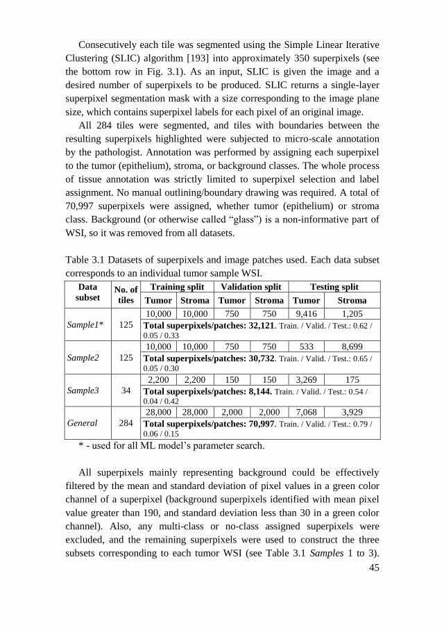
45
Consecutively each tile was segmented using the Simple Linear Iterative
Clustering (SLIC) algorithm [193] into approximately 350 superpixels (see
the bottom row in Fig. 3.1). As an input, SLIC is given the image and a
desired number of superpixels to be produced. SLIC returns a single-layer
superpixel segmentation mask with a size corresponding to the image plane
size, which contains superpixel labels for each pixel of an original image.
All 284 tiles were segmented, and tiles with boundaries between the
resulting superpixels highlighted were subjected to micro-scale annotation
by the pathologist. Annotation was performed by assigning each superpixel
to the tumor (epithelium), stroma, or background classes. The whole process
of tissue annotation was strictly limited to superpixel selection and label
assignment. No manual outlining/boundary drawing was required. A total of
70,997 superpixels were assigned, whether tumor (epithelium) or stroma
class. Background (or otherwise called “glass”) is a non-informative part of
WSI, so it was removed from all datasets.
Table 3.1 Datasets of superpixels and image patches used. Each data subset
corresponds to an individual tumor sample WSI.
Data
subset No. of
tiles
Training split Validation split Testing split
Tumor Stroma Tumor Stroma Tumor Stroma
Sample1* 125
10,000 10,000 750 750 9,416 1,205
Total superpixels/patches: 32,121. Train. / Valid. / Test.: 0.62 /
0.05 / 0.33
Sample2 125
10,000 10,000 750 750 533 8,699
Total superpixels/patches: 30,732. Train. / Valid. / Test.: 0.65 /
0.05 / 0.30
Sample3 34
2,200 2,200 150 150 3,269 175
Total superpixels/patches: 8,144. Train. / Valid. / Test.: 0.54 /
0.04 / 0.42
General 284
28,000 28,000 2,000 2,000 7,068 3,929
Total superpixels/patches: 70,997. Train. / Valid. / Test.: 0.79 /
0.06 / 0.15
* - used for all ML model’s parameter search.
All superpixels mainly representing background could be effectively
filtered by the mean and standard deviation of pixel values in a green color
channel of a superpixel (background superpixels identified with mean pixel
value greater than 190, and standard deviation less than 30 in a green color
channel). Also, any multi-class or no-class assigned superpixels were
excluded, and the remaining superpixels were used to construct the three
subsets corresponding to each tumor WSI (see Table 3.1 Samples 1 to 3).
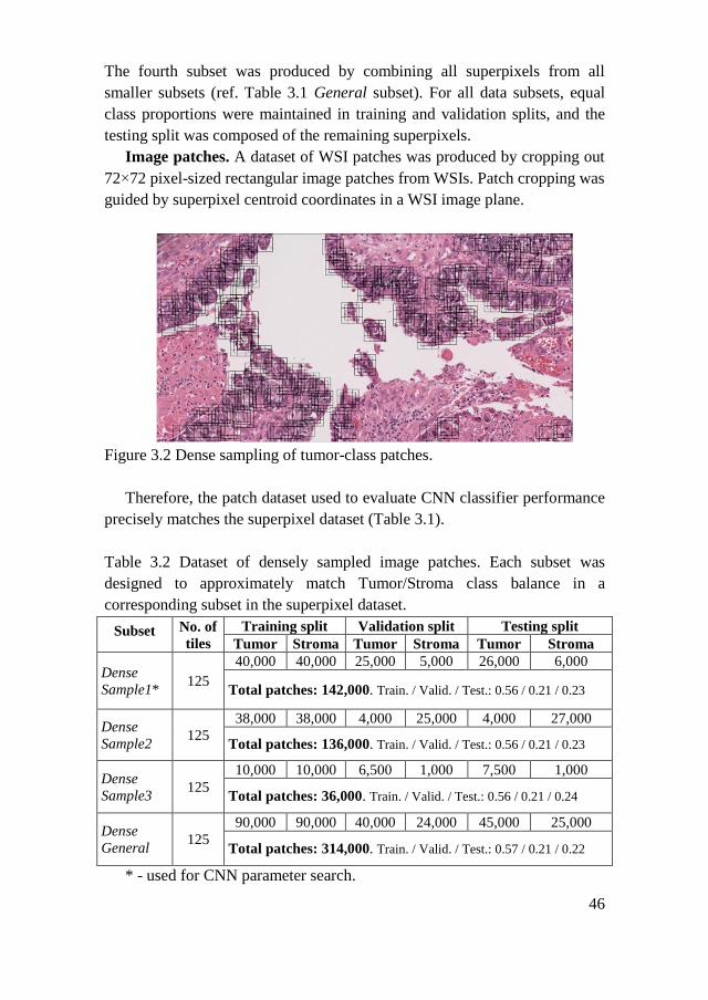
46
The fourth subset was produced by combining all superpixels from all
smaller subsets (ref. Table 3.1 General subset). For all data subsets, equal
class proportions were maintained in training and validation splits, and the
testing split was composed of the remaining superpixels.
Image patches. A dataset of WSI patches was produced by cropping out
72×72 pixel-sized rectangular image patches from WSIs. Patch cropping was
guided by superpixel centroid coordinates in a WSI image plane.
Figure 3.2 Dense sampling of tumor-class patches.
Therefore, the patch dataset used to evaluate CNN classifier performance
precisely matches the superpixel dataset (Table 3.1).
Table 3.2 Dataset of densely sampled image patches. Each subset was
designed to approximately match Tumor/Stroma class balance in a
corresponding subset in the superpixel dataset.
Subset No. of
tiles
Training split Validation split Testing split
Tumor Stroma Tumor Stroma Tumor Stroma
Dense
Sample1* 125
40,000 40,000 25,000 5,000 26,000 6,000
Total patches: 142,000. Train. / Valid. / Test.: 0.56 / 0.21 / 0.23
Dense
Sample2 125
38,000 38,000 4,000 25,000 4,000 27,000
Total patches: 136,000. Train. / Valid. / Test.: 0.56 / 0.21 / 0.23
Dense
Sample3 125
10,000 10,000 6,500 1,000 7,500 1,000
Total patches: 36,000. Train. / Valid. / Test.: 0.56 / 0.21 / 0.24
Dense
General 125
90,000 90,000 40,000 24,000 45,000 25,000
Total patches: 314,000. Train. / Valid. / Test.: 0.57 / 0.21 / 0.22
* - used for CNN parameter search.

47
Additionally, annotated superpixel centroids were used to densely sample
data and generate patches for CNN classification on the augmented dataset
(given in Table 3.2). Five overlapping 72×72 pixels RGB patches were
selected in the original image around each superpixel mass centre by shifting
the frame in each of the four directions (0°, 90°, 180°, 270°) by 15 pixels
(Figure 3.2).
3.1.2. Superpixel Descriptors
RGB superpixels. Superpixels in each subset were bound in a rectangle
minimum bounding box, keeping the three color channels. Pixels inside the
bounding box, but outside the superpixel area were assigned zero values in
each color channel.
Grayscale superpixels. Superpixels in each subset were bound in a
rectangle minimum bounding box. Zero values were assigned to the pixels
inside the bounding box, but outside the superpixel area, and converted to
grayscale. A color-to-grayscale transformation that retains the Luminance of
the original image was chosen. A detailed review of color-to-grayscale
transformations frequently used in computer vision emphasizes that
Luminance is considered a good choice for texture recognition [194].
Color-based descriptors. For each grayscale superpixel, two statistics
were calculated – mean and standard deviation of the pixel value. For an
RGB superpixel, eight statistics were calculated – mean and standard
deviation of the pixel value for each color channel separately and also all
RGB color channels.
Image texture-based descriptors. The texture of a grayscale superpixel
has been measured by calculating the spatial gray-level co-occurrence matrix
[58] for four directions (at 1 px displacement vector). The 13 directions for
an RGB superpixel were used. From each of the resulting co-occurrence
matrices, 13 parameters were calculated as follows: angular second moment,
contrast, correlation, the sum of squares, inverse difference moment, sum
average, sum variance, sum entropy, entropy, difference variance, difference
entropy, information measure of correlation 1, and information measure of
correlation 2. For each parameter mean value was obtained from all
directions, thus resulting in the final 13 descriptors. To extract texture
descriptors Python computer vision and image processing library Mahotas
[195] was used.
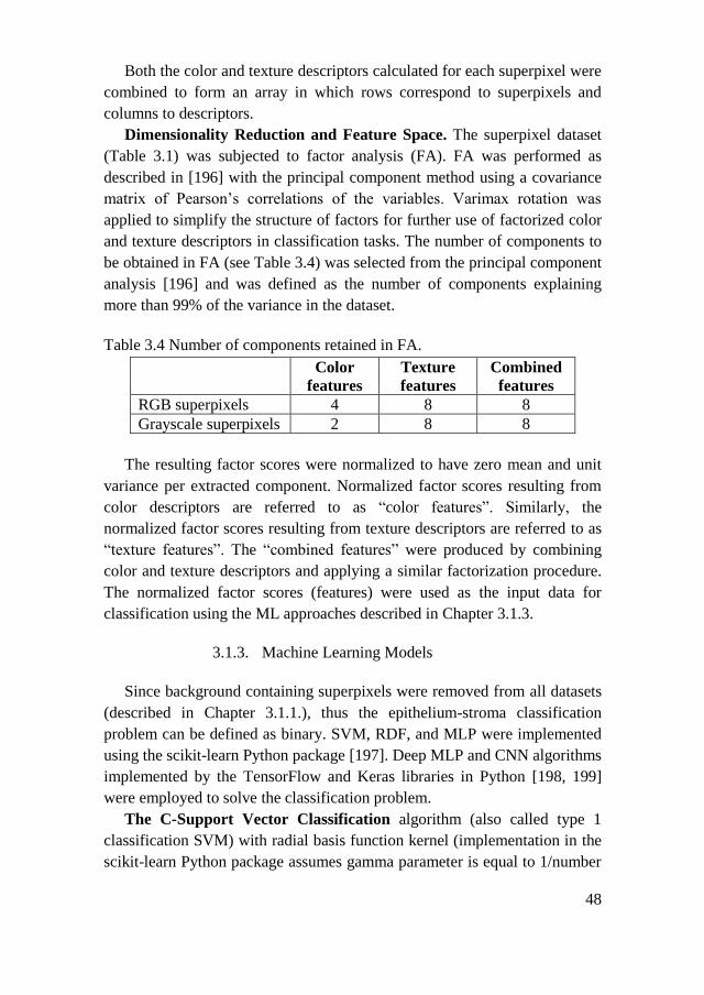
48
Both the color and texture descriptors calculated for each superpixel were
combined to form an array in which rows correspond to superpixels and
columns to descriptors.
Dimensionality Reduction and Feature Space. The superpixel dataset
(Table 3.1) was subjected to factor analysis (FA). FA was performed as
described in [196] with the principal component method using a covariance
matrix of Pearson’s correlations of the variables. Varimax rotation was
applied to simplify the structure of factors for further use of factorized color
and texture descriptors in classification tasks. The number of components to
be obtained in FA (see Table 3.4) was selected from the principal component
analysis [196] and was defined as the number of components explaining
more than 99% of the variance in the dataset.
Table 3.4 Number of components retained in FA.
Color
features
Texture
features
Combined
features
RGB superpixels 4 8 8
Grayscale superpixels 2 8 8
The resulting factor scores were normalized to have zero mean and unit
variance per extracted component. Normalized factor scores resulting from
color descriptors are referred to as “color features”. Similarly, the
normalized factor scores resulting from texture descriptors are referred to as
“texture features”. The “combined features” were produced by combining
color and texture descriptors and applying a similar factorization procedure.
The normalized factor scores (features) were used as the input data for
classification using the ML approaches described in Chapter 3.1.3.
3.1.3. Machine Learning Models
Since background containing superpixels were removed from all datasets
(described in Chapter 3.1.1.), thus the epithelium-stroma classification
problem can be defined as binary. SVM, RDF, and MLP were implemented
using the scikit-learn Python package [197]. Deep MLP and CNN algorithms
implemented by the TensorFlow and Keras libraries in Python [198, 199]
were employed to solve the classification problem.
The C-Support Vector Classification algorithm (also called type 1
classification SVM) with radial basis function kernel (implementation in the
scikit-learn Python package assumes gamma parameter is equal to 1/number
49
of features) was used [200]. With SVM classification is achieved by
constructing hyperplane in multidimensional space to separate instances of
different classes. Error minimization is employed in an iterative algorithm to
find optimal hyperplane. Nonlinear classification is achieved by using kernel
functions of which radial basis function is the most common choice [201].
An RDF classifier is a perturb-and-combine technique specifically
designed for classification trees [48]. The principle is based on
randomization – a bootstrap sample is drawn from a training set to build
each of the trees, and the split on the node is chosen as the best split among a
random subset of the features. A predictor of RDF can be selected in a
voting procedure or by averaging individual tree probabilistic predictions.
Methods that use averaging are known to have relatively high variance due
to feature subsetting at the base level. Thus, after classification with RDF, a
separate calibration of predicted probabilities was performed as post-
processing using the sigmoid method and validation datasets (disjoint data
used for training and calibration). In the RDF classifier, 25 estimators (base-
level trees) were selected by calibration (no observed significant difference
in performance between 25 and 1,000 estimators used) and the maximum
number of features to be used with an individual tree was defined to be
integer square root of the total number of features. The nodes were expanded
until all leaves had at least two samples. All the input samples had equal
weight.
MLP is a feedforward neural network (a network whose neurons are
connected only in a forward manner to form layers) that is trained by
backpropagation [45]. Neurons in the network consist of the linear combiner
and an activation function. In the model the rectifier activation function
[202] was used – a function whose output is equal to the input if the input is
positive, otherwise, the output is set to 0. The network was constituted of
one input layer containing inputs corresponding to the features in the dataset,
of two hidden layers with 1,000 and 40 neurons respectively, and of an
output layer with a single neuron. The number of neurons in hidden layers
was selected empirically. Network performance was tested increasing
number of neurons in both hidden layers from 100 and 10 up to 1,000 and 40
respectively. Classifier performance was stable among all tested
architectures with a mean variation of the area under the receiver operating
characteristic curve (AUC) being less than 0.0003. Connections between
layers are defined by weights assigned in the learning process, and each
neuron in a layer is connected to every neuron in the next layer. In a training
phase, an output of the network (a probability matrix instead of discrete

50
predictions) in an iterative manner is compared to GT labels of the input
data, and a cross-entropy loss is computed as a negative log-likelihood of a
classifier. The model uses the limited-memory Broyden–Fletcher–Goldfarb–
Shanno (LBFGS) method to optimize log-loss function with respect to the
network parameters as a default optimizer. LBFGS is an optimizer in the
family of quasi-Newton methods [203]. The training phase is ended if the
validation log-loss is not improving by at least a predefined amount (here
0.0001) for two consecutive iterations, or when a predefined number of
iterations (here 200) had been reached.
The deep MLP is a feedforward neural network with multiple hidden
layers between the input and output layers that is trained by
backpropagation. The basic difference between deep MLP and MLP used in
this chapter is that the deep MLP network is constructed of more hidden
layers and more neurons per layer. The deep MLP network was constructed
with three fully connected layers (with the corresponding number of neurons
– 1,024, 512, 128). Neurons in the network use the rectifier activation
function (the same as in MLP). Between the last hidden layer and an output
layer, a dropout layer was added. Dropout is a regularization technique for
reducing overfitting in the model, by omitting a specified proportion (50% in
this case) of random neurons output. An output layer has two neurons that
use the softmax activation function – a function that given a vector outputs a
probability distribution over all possible outcomes (in this case 2 –
corresponding to two tissue classes). A number of neurons in all three hidden
layers were selected by calibration. The network performance was tested for
three configurations regarding the number of neurons in hidden layers (1,024
/ 512 / 128, 2,048 / 1,024 / 256 and 5,120 / 2,560 / 640). Classifier
performance was stable for both tested architectures with a mean variation of
AUC being less than 0.002, therefore the network architecture with the
lowest complexity was selected. Log-loss of the model is computed as
described in MLP. The network is trained using the adaptive moment
estimation (Adam [204]) method with an adjusted learning rate (0.000001)
to minimize the cross-entropy loss function. The training phase is ended if
the validation log-loss does not improve for ten consecutive iterations, or
when a predefined number of iterations (here 200) had been reached.
CNNs are a variation of deep learning neural networks. They employ
a local connectivity pattern in the data; thus, weight-sharing between
neurons of adjacent layers becomes possible. Every convolutional layer of
CNN transforms one volume of activations to another through a
differentiable function. Neurons in a layer are only connected to a small

51
region of the layer before it (a tensor) through a set of weights (a filter) and
are distributed along with the depth of a tensor. In a filtering operation the
filter is slid over a tensor with a fixed size stride. Filtering inside a layer is a
discrete convolution. Thus, the spatial output decreases with each layer. To
reduce the number of parameters in the network a pooling operation is
employed. Pooling combines the outputs of a group of neurons in one layer
into a single neuron in the next layer. The output of the last convolutional
layer is flattened and fed into the dense layers of the network. The dense
layer or fully connected layer is similar to a hidden layer of an MLP. A
relatively simple CNN was constructed to classify image patches. The
prostate cancer detection study by Litjens et al. [94] introduced the deep
learning techniques to digital pathology employing similar CNN
architecture. The model consists of four convolutional layers, one fully
connected layer and an output layer with two neurons and a softmax
activation function (see Table 3.4). Filter sizes and strides were adjusted to
accept 72×72 pixel patches and batch normalization layers were added after
each conv2d layer. The Adam method with an adjusted learning rate
(0.000001) was used to minimize cross-entropy loss function. The training
phase is ended if the validation log-loss is not improving for ten consecutive
iterations, or when a predefined number of iterations (here 200) had been
reached. The network’s width (number of neurons in hidden layers) was
selected by calibration (see Table 3.4 for results) by training and evaluation
using Dense Sample1 data subset (see Table 3.2).
Table 3.4 Parameters of CNN tested. Number of feature maps. The best
performing model configuration is bolded in the table and was used in
further analyses.
Number of neurons in hidden layers Performance
metrics
conv2d
1
conv2d
2
conv2d
3
conv2d
4
fully
connected
Mean
AUC
std
AUC
32 32 64 64 384 0.9704 0.0007
32 32 64 64 1024 0.9667 0.0005
64 64 128 128 384 0.9726 0.0004
64 64 128 128 1024 0.9687 0.0008
96 96 192 192 384 0.9745 0.0003
96 96 192 192 1024 0.9721 0.0003
52
Ten iterations were used to train and test CNN, each time randomly
assigning the data to the training, validation and testing splits with exactly
the same proportions of class labels.
3.2. Results
Typically, classifier prediction is a numeric value on a continuous scale.
A class label is produced by comparing a prediction (or a score) to a
threshold value. After training ML classifiers on training and validation
splits, the testing split was used to evaluate each model performance by
calculating AUC. An SVM, RDF, MLP, and deep MLP models were trained
and evaluated using color and texture features (factorized descriptors
described in Chapter 3.1.2) produced from the superpixel dataset (see Table
3.1). CNN was trained on a matched image patches dataset as well as a
densely sampled image patches dataset (see Table 3.2).
Ten iterations were used to train and test all the classifiers, each time
randomly assigning the data to the training and testing subsets with the same
proportions of class labels. Mean AUC and the standard deviation of AUC
were calculated for each of the classifiers. Both RGB and grayscale datasets
were used to evaluate ML models. The results are summarized in Tables 3.5
and 3.6.
Superpixel dataset classification. In single Sample data subsets, ML
classifier results on RGB superpixel features (Table 3.5) range from 0.9095
up to 0.9769 (by AUC). All ML models performed quite similarly - no
particular model stands out as exceptionally better than others. However,
MLP achieved the best generalization among traditional ML-based
classifiers (AUC = 0.9666), also outperforming deep MLP (AUC = 0.9575).
Classification results for grayscale superpixels (Table 3.6) differ more
substantially. For these experimental conditions, AUC scores achieved were
in a range between 0.5533 and 0.9443. However, this difference was
observed between the Samples data subsets, but not between the ML models.
Interestingly, data subset size did not affect classifier performance.
Contrary to what was expected, classification accuracies on the Sample3 data
subset are comparable to the results of larger data subsets (e.g., the Sample1
data subset is nearly four-fold larger than Sample3) for RGB superpixels (see
Table 3.5) and even better for grayscale superpixels (Table 3.6). This finding
suggests that individual characteristics of the tissue sample were the cause of
the variation in the results.

Table 3.5 Classifier performance of RGB superpixels/patches. Results are given as mean AUC ± standard deviation of AUC
acquired in 10 repetitions. Gray background marked cells indicate the best result for each data subset.
RGB
Sample1 Sample2 Sample3 General
Colo
r
Com
bin
ed
Tex
ture
Colo
r
Com
bin
ed
Tex
ture
Colo
r
Com
bin
ed
Tex
ture
Colo
r
Com
bin
ed
Tex
ture
RDF 0.9453
±0.0046
0.9413
±0.0044
0.9095
±0.0051
0.9609
±0.0049 0.9725
±0.0058
0.9548
±0.0077
0.9343
±0.0057 0.9473
±0.0067
0.9427
±0.0055
0.9466
±0.0023 0.9533
±0.0022
0.9385
±0.0035
SVM 0.9534
±0.0040
0.9505
±0.0045
0.9265
±0.0035
0.9695
±0.0042 0.9769
±0.0025
0.9620
±0.0029
0.9441
±0.0073 0.9534
±0.0066
0.9483
±0.0048
0.9515
±0.0014 0.9620
±0.0024
0.9488
±0.0021
MLP 0.9526
±0.0050
0.9387
±0.0043
0.9107
±0.0060
0.9683
±0.0034 0.9713
±0.0039
0.9586
±0.0040
0.9217
±0.0071 0.9333
±0.0051
0.9282
±0.0049
0.9577
±0.0031 0.9666
±0.0026
0.9542
±0.0031
deep
MLP 0.9535
±0.0049
0.9480
±0.0042
0.9105
±0.0055
0.9701
±0.0114 0.9764
±0.0148
0.9629
±0.0145
0.9320
±0.0060 0.9392
±0.0080
0.9345
±0.0070
0.9556
±0.0026 0.9575
±0.0019
0.9449
±0.0040
CNN
patches 0.8942 ±0.0067 0.9681 ±0.0028 0.9477 ±0.0093 0.9895 ±0.0006
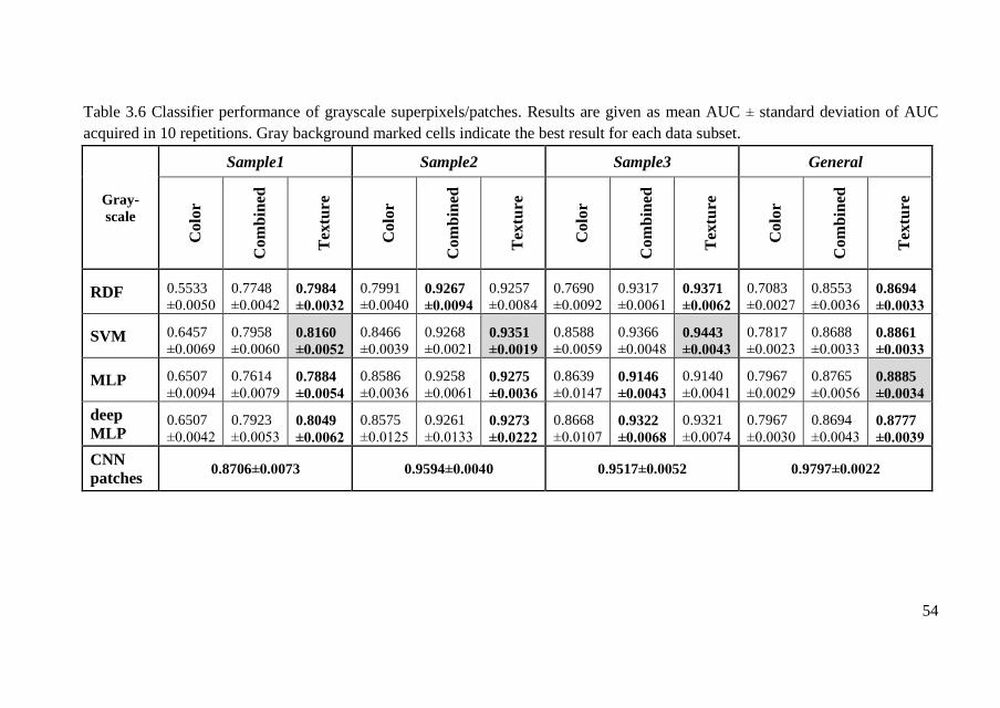
54
Table 3.6 Classifier performance of grayscale superpixels/patches. Results are given as mean AUC ± standard deviation of AUC
acquired in 10 repetitions. Gray background marked cells indicate the best result for each data subset.
Gray-
scale
Sample1 Sample2 Sample3 General
Colo
r
Com
bin
ed
Tex
ture
Colo
r
Com
bin
ed
Tex
ture
Colo
r
Com
bin
ed
Tex
ture
Colo
r
Com
bin
ed
Tex
ture
RDF 0.5533
±0.0050
0.7748
±0.0042 0.7984
±0.0032
0.7991
±0.0040 0.9267
±0.0094
0.9257
±0.0084
0.7690
±0.0092
0.9317
±0.0061 0.9371
±0.0062
0.7083
±0.0027
0.8553
±0.0036 0.8694
±0.0033
SVM 0.6457
±0.0069
0.7958
±0.0060 0.8160
±0.0052
0.8466
±0.0039
0.9268
±0.0021 0.9351
±0.0019
0.8588
±0.0059
0.9366
±0.0048 0.9443
±0.0043
0.7817
±0.0023
0.8688
±0.0033 0.8861
±0.0033
MLP 0.6507
±0.0094
0.7614
±0.0079 0.7884
±0.0054
0.8586
±0.0036
0.9258
±0.0061 0.9275
±0.0036
0.8639
±0.0147 0.9146
±0.0043
0.9140
±0.0041
0.7967
±0.0029
0.8765
±0.0056 0.8885
±0.0034
deep
MLP 0.6507
±0.0042
0.7923
±0.0053 0.8049
±0.0062
0.8575
±0.0125
0.9261
±0.0133 0.9273
±0.0222
0.8668
±0.0107 0.9322
±0.0068
0.9321
±0.0074
0.7967
±0.0030
0.8694
±0.0043 0.8777
±0.0039
CNN
patches 0.8706±0.0073 0.9594±0.0040 0.9517±0.0052 0.9797±0.0022
The nature of the feature space has the largest effect on superpixel
classification. Extracted color features proved to be exclusively valuable. For
RGB superpixels (see Table 3.5), color or color combined with texture
features provide the best results. The best AUC for individual Samples data
subsets achieved were in the range between 0.9534 and 0.9769 (with AUC =
0.9666 under generalization conditions). Combining color and texture
features increased classification accuracy for RGB superpixels (AUC =
0.9666) when compared to color features alone (AUC = 0.9577) or texture
features alone (AUC = 0.9542) under generalization conditions.
Grayscale superpixels carry less color information. Therefore, in most
cases, texture features of grayscale superpixels allow better classification
(AUC in the range between 0.8160 and 0.9443) than color or combined
features (see Table 3.6).
The best performance on the General data subset was observed with MLP
and texture features (AUC = 0.8885), which is substantially lower when
compared to the best result of RGB superpixels (with MLP and combined
features, AUC = 0.9666). The results align well with results published by
other groups for feature space-based ML classifiers: AUC 0.97 – 0.99 [144]
and AUC = 0.98 [147] both targeting colorectal cancer, and AUC = 0.98
[91] on prostate cancer images.
Image patch CNN classification. CNN classifier trained on RBG image
patches achieved 0.9895 AUC under generalization conditions. This result is
comparable to results achieved by other groups for breast cancer (AUC =
0.9316) [95], and prostate cancer (AUC = 0.965 and AUC = 0.99) [91, 94].
Under these experimental conditions, CNN classification accuracy was
significantly higher than other ML models trained on RGB superpixel
features (AUC = 0.9895 against 0.9533 – 0.9666 achieved with other ML
models).
However, for individual Samples data subsets CNN did not perform
better than other ML models trained on RGB superpixel features (e.g., SVM
achieved AUC 0.9534 – 0.9769 and CNN achieved AUC 0.8942 – 0.9681,
see Table 3.6).
When trained on grayscale image patches CNN in all cases was more
accurate (AUC in the range between 0.8706 and 0.9797) than other ML
models trained on grayscale superpixel features (AUC in the range between
0.8160 and 0.9443), but less accurate than CNN trained on RGB patches
(AUC in the range between 0.8942 and 0.9895).
Augmentation of the image patches dataset by dense sampling did not
significantly improve the classification results. An improvement was
observed for the Sample1 data subset (AUC = 0.9745 for the dense RGB
56
dataset, AUC = 0.8942 for matched RGB subset; AUC = 0.9338 for the
dense grayscale subset, AUC = 0.8706 for matched grayscale subset).
However, no improvement was observed for the Sample2 data subset, and a
decrease in classification accuracy was observed for the Sample3 data subset
(AUC = 0.8939 for the densely sampled RGB patches, AUC = 0.9477 for
matched RGB patches; AUC = 0.8993 for the densely sampled grayscale
patches, AUC = 0.9517 for matched grayscale patches). Dense sampling by
shifting around a superpixel centroid might have created an unwanted
mixing of the classes. It can again be hypothesized that individual
characteristics of the tissue sample were the cause of the variation in the
results. This finding is concordant with the observed variation in results
regarding the size of superpixels subsets.
3.3. Chapter Conclusions
The tumor tissue classification was approached by annotated superpixel
classification using conventional classifiers, and the classification by CNN
of patched image data. The following conclusions are drawn:
Superpixel color features allow better classification results (AUC 0.9217
– 0.9701) compared to texture features (AUC 0.9095-0.9629) in all data
subsets. Under generalization conditions, combining color and texture
features increased the classification accuracy of all ML models on RGB
superpixels dataset (AUC = 0.9533 – 0.9666) when compared to color
features alone (AUC = 0.9466 – 0.9577) or texture features alone (AUC =
0.9385 – 0.9542).
As expected, CNN achieved the best overall classification generalization
(AUC = 0.9895). Interestingly, even when trained on grayscale image
patches CNN achieved better generalization (AUC = 0.9797) than other ML
models trained on RGB superpixel features (AUC 0.9533 – 0.9666). This
suggests that by learning directly from image data CNN can build a diverse
feature space in hidden layers of its architecture.
57
4. METHOD FOR CELL NUCLEI SEGMENTATION WITH
LYMPHOCYTE IDENTIFICATION
The previous chapter focused on the identification of two major tumor
tissue compartments – tumor epithelium and stroma. This chapter even
further explores the H&E-stained tissue WSI analysis, i.e. the detection of
lymphocytes – immune cells that often move along tumor compartment
margins (TILS – tumor-infiltrating lymphocytes). Lymphocyte segmentation
in a set of H&E-stained breast cancer and colorectal cancer tissue images is
considered. The motivation to specifically target lymphocytes stems from
the fact that lymphocyte segmentation in routine pathology images is a
necessary but underresearched topic in digital pathology (reviewed in
Chapter 2.2.3).
4.1. Experiment Design
This chapter introduces a model for cell nuclei segmentation. An
extension of the FCNN-based state-of-the-art cell segmentation models is
considered. The idea of a multiple-resolution image input architecture is
adopted from the Micro-Net model [104] and the multi-level interconnected
architecture of the U-Net [99] is used as a base model for the segmentation
of all types of tissue nuclei. A new structuring element of the network
architecture is introduced (named “texture block”). The texture block
consists of 2 parallel chains of 3 convolution layers, which enhance image
texture extraction. An increase in segmentation performance is expected.
The segmentation performance of the proposed model is compared against
higher complexity models such as U-Net and Micro-Net.
Additionally, the separation of clumped cell nuclei is considered. An
active contour layer is added to the GT images, and the nuclei segmentation
model is trained to output both segmented nuclei and the contour of each
nucleus. Again, an increase in segmentation performance is expected.
After segmentation, lymphocyte identification in a set of segmented
nuclei by an ML-based classification is considered. Classification accuracy,
precision, recall, and F1-score of an RDF classifier, MLP, and CNN are
compared.
The schema of the proposed method is summarized in Figure 4.1. After
careful hyperparameter tuning and model training, the method assumes a
trained nuclei segmentation model to accept new images and produce
segmentation masks (Fig. 4.1 step 1B). The resulting segmentation masks
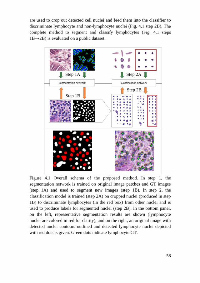
58
are used to crop out detected cell nuclei and feed them into the classifier to
discriminate lymphocyte and non-lymphocyte nuclei (Fig. 4.1 step 2B). The
complete method to segment and classify lymphocytes (Fig. 4.1 steps
1B→2B) is evaluated on a public dataset.
Figure 4.1 Overall schema of the proposed method. In step 1, the
segmentation network is trained on original image patches and GT images
(step 1A) and used to segment new images (step 1B). In step 2, the
classification model is trained (step 2A) on cropped nuclei (produced in step
1B) to discriminate lymphocytes (in the red box) from other nuclei and is
used to produce labels for segmented nuclei (step 2B). In the bottom panel,
on the left, representative segmentation results are shown (lymphocyte
nuclei are colored in red for clarity), and on the right, an original image with
detected nuclei contours outlined and detected lymphocyte nuclei depicted
with red dots is given. Green dots indicate lymphocyte GT.
Step 1A
Step 1B
Step 2A
Step 2B
59
4.1.1. Datasets
Images. In this experiment, 4 whole-slide histology sample images
prepared with H&E staining were used (2 WSI slides from breast cancer
patients and 2 WSIs from colorectal cancer). These slides were produced in
the National Center of Pathology, Lithuania (NCP), and digitized with the
Aperio ScanScope XT Slide Scanner at 20× magnification. 1 WSI slide was
obtained from the TCGA database [205], tile ID: TCGA_AN_A0AM, and
used for both segmentation and classification testing.
For the results and approach validation, two additional public collections
of annotated histology images were used - the CRCHistoPhenotypes dataset
[153] (CRCHP) and the breast cancer dataset [155] (JAN). CRCHP contains
100 H&E-stained colorectal cancer histology images (500×500 pixel-sized
excerpts from WSIs) with identified cell nuclei. The CRCHP dataset entails
broad cell type categories, where lymphocytes are annotated under the
inflammatory label. The JAN dataset consists of 100 H&E-stained breast
cancer histology images (100×100 pixel-sized excerpts from WSIs) with
only lymphocytes annotated.
All images (both public and private) were acquired using 20×
magnification and annotated by an expert pathologist marking lymphocyte
nuclei centers.
The described images were used to generate two diverse datasets
dedicated to segmentation and classification tasks. Both datasets are
summarized in Table 4.1 and Table 4.3 and described in the following
paragraphs.
Segmentation dataset. To train and validate the segmentation model,
randomly selected 344 tiles of 256×256 pixel size were used. Dataset was
split into training and validation sets, respectively. To test the segmentation
model, 96 tiles from the breast cancer TCGA slide were produced. Both tiles
generated from the TCGA slide and tiles generated from NCP slides were
manually annotated. In the annotation process, each cell nucleus present in
an image patch was manually outlined, and 2 pixel-wide active contour
borders surrounding each nucleus were added as a second layer to the nuclei
segmentation masks. Each outlined nucleus was assigned a class label (a
lymphocyte or other).
Tiles generated from WSIs (NCP and TCGA) were converted into
floating-point data type, and their values were scaled to the unit interval [0,
1] channel-wise. Various image augmentation methods (rotation, flip,
transpose, RGB augmentation, brightness adjustment, CLAHE [206]) were
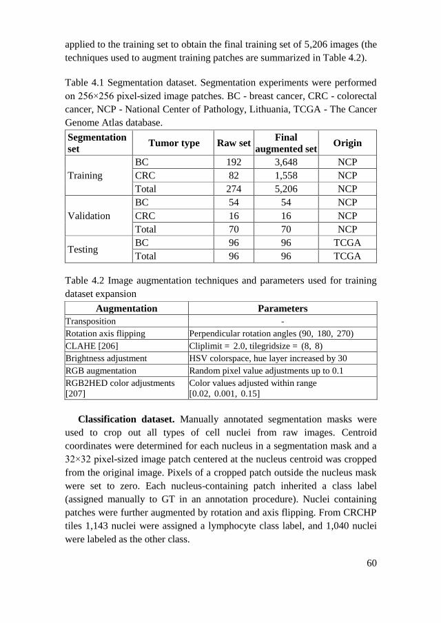
60
applied to the training set to obtain the final training set of 5,206 images (the
techniques used to augment training patches are summarized in Table 4.2).
Table 4.1 Segmentation dataset. Segmentation experiments were performed
on 256×256 pixel-sized image patches. BC - breast cancer, CRC - colorectal
cancer, NCP - National Center of Pathology, Lithuania, TCGA - The Cancer
Genome Atlas database.
Segmentation
set Tumor type Raw set
Final
augmented set Origin
Training
BC 192 3,648 NCP
CRC 82 1,558 NCP
Total 274 5,206 NCP
Validation
BC 54 54 NCP
CRC 16 16 NCP
Total 70 70 NCP
Testing BC 96 96 TCGA
Total 96 96 TCGA
Table 4.2 Image augmentation techniques and parameters used for training
dataset expansion
Augmentation Parameters
Transposition -
Rotation axis flipping Perpendicular rotation angles (90, 180, 270)
CLAHE [206] Cliplimit = 2.0, tilegridsize = (8, 8)
Brightness adjustment HSV colorspace, hue layer increased by 30
RGB augmentation Random pixel value adjustments up to 0.1
RGB2HED color adjustments
[207]
Color values adjusted within range
[0.02, 0.001, 0.15]
Classification dataset. Manually annotated segmentation masks were
used to crop out all types of cell nuclei from raw images. Centroid
coordinates were determined for each nucleus in a segmentation mask and a
32×32 pixel-sized image patch centered at the nucleus centroid was cropped
from the original image. Pixels of a cropped patch outside the nucleus mask
were set to zero. Each nucleus-containing patch inherited a class label
(assigned manually to GT in an annotation procedure). Nuclei containing
patches were further augmented by rotation and axis flipping. From CRCHP
tiles 1,143 nuclei were assigned a lymphocyte class label, and 1,040 nuclei
were labeled as the other class.

61
Table 4.3 Classification dataset. Classification experiments were performed
on extracted cell nuclei embedded in blank 32×32 pixel-sized placeholders.
BC - breast cancer, CRC - colorectal cancer, NCP - National Center of
Pathology, Lithuania, TCGA - The Cancer Genome Atlas database, CRCHP
- CRCHistoPhenotypes dataset [153], JAN - the breast cancer dataset [155].
Classification
set Nucleus type Raw set
Final
augmented set Origin
Training
Lymphocyte
nuclei
11,032 50,950
NCP Other nuclei 10,922 55,825
Total nuclei 21,954 106,775
Validation
Lymphocyte
nuclei
2,588 2,588
NCP Other nuclei 2,751 2,751
Total nuclei 5,339 5,339
Testing
BC lymphocytes 903 903 TCGA
CRC lymphocytes 1,143 1,143 CRCHP
Total lymphocytes 2,046 2,046 TCGA +
CRCHP
BC other 1,195 1,195 TCGA
CRC other 1,040 1,040 CRCHP
Total other 2,235 2,235 TCGA +
CRCHP
Total nuclei 4,281 4,281 TCGA +
CRCHP
Evaluation
BC lymphocytes 2,949 2,949
JAN BC other 1,921 1,921
Total nuclei 4,870 4,870
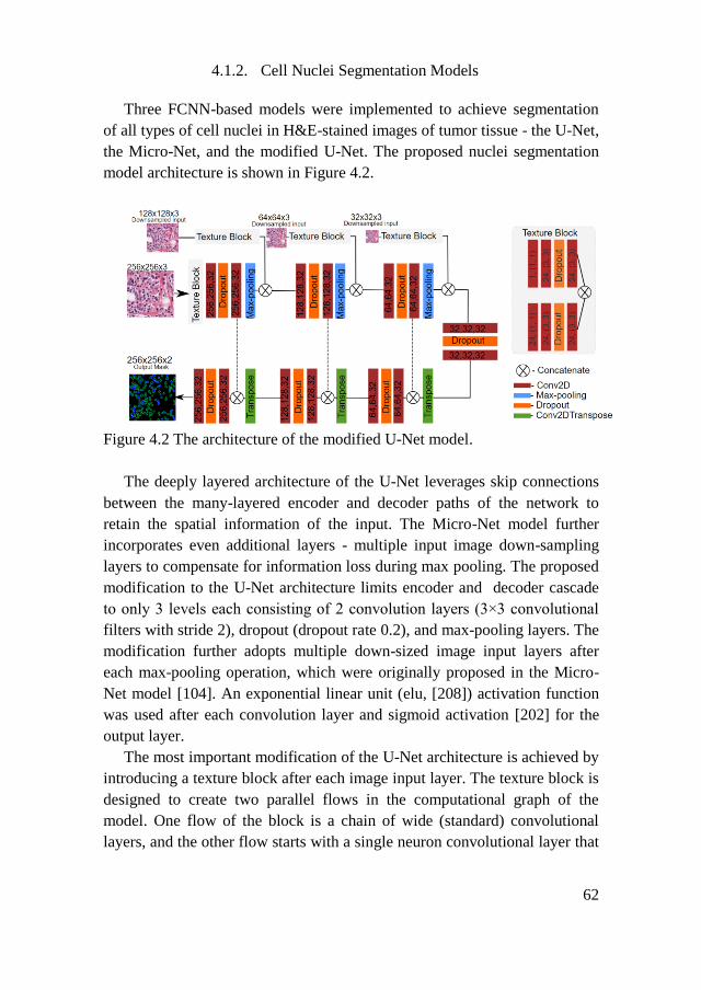
62
4.1.2. Cell Nuclei Segmentation Models
Three FCNN-based models were implemented to achieve segmentation
of all types of cell nuclei in H&E-stained images of tumor tissue - the U-Net,
the Micro-Net, and the modified U-Net. The proposed nuclei segmentation
model architecture is shown in Figure 4.2.
Figure 4.2 The architecture of the modified U-Net model.
The deeply layered architecture of the U-Net leverages skip connections
between the many-layered encoder and decoder paths of the network to
retain the spatial information of the input. The Micro-Net model further
incorporates even additional layers - multiple input image down-sampling
layers to compensate for information loss during max pooling. The proposed
modification to the U-Net architecture limits encoder and decoder cascade
to only 3 levels each consisting of 2 convolution layers (3×3 convolutional
filters with stride 2), dropout (dropout rate 0.2), and max-pooling layers. The
modification further adopts multiple down-sized image input layers after
each max-pooling operation, which were originally proposed in the Micro-
Net model [104]. An exponential linear unit (elu, [208]) activation function
was used after each convolution layer and sigmoid activation [202] for the
output layer.
The most important modification of the U-Net architecture is achieved by
introducing a texture block after each image input layer. The texture block is
designed to create two parallel flows in the computational graph of the
model. One flow of the block is a chain of wide (standard) convolutional
layers, and the other flow starts with a single neuron convolutional layer that

63
is expected to create a bottleneck in the architecture and force the
propagation of different convolutional features.
Adam optimizer [204] was used with initial learning rate lr = 0.001,
which was reduced by factor 0.1 if validation loss did not improve for 4
consecutive epochs (the lower limit of learning rate was set to 1×10⁻⁶). Dice
coefficient (4.1) in combination with binary cross-entropy loss (4.2) was
used to quantify model metrics as a custom loss function (4.3) [209, 210].
𝐷𝑖𝑐𝑒 =2∗𝑇𝑃
(𝑇𝑃+𝐹𝑃)+(𝑇𝑃+𝐹𝑁) (4.1)
where TP is true positive, FP is false positive and FN is false
negative.
𝐿(𝑦, �̂�) = −(𝑦 ∗ log(�̂�) + (1 − 𝑦) ∗ log(1 − �̂�)) (4.2)
where 𝑦 is a binary class label and �̂� is predicted probability.
𝐶𝑟𝑜𝑠𝑠𝑒𝑛𝑡𝑟𝑜𝑝𝑦𝐷𝑖𝑐𝑒𝐿𝑜𝑠𝑠 = 0.1 ∗ 𝐿(𝑦, �̂�) + 0.9 ∗ (1 − 𝐷𝑖𝑐𝑒) (4.3)
Figure 4.3 Training of the proposed U-Net architecture.
Model converged after 36 epochs (see Fig. 4.3) using a batch size of 1
(input image dimensions: 256×256×3) for training and validation.
64
4.1.3. Cell Nuclei Classifiers
The cell nuclei classification problem was approached with RDF, MLP,
and CNN classifiers.
RDF was chosen as a baseline ML algorithm. RDF was used with the
Gini impurity criterion as split quality measurement and 10 estimators. The
RDF classifier was trained on linearized nuclei images (32×32 RGB-colored
images linearized to 3,072-length vector), which achieved 0.77 testing
accuracy.
The MLP model employed consists of three dense layers (number of
nodes: 4096, 2048, 1024), with softmax as the output layer activation
function. For each layer, relu activation was used, followed by batch
normalization. The dropout layer (dropout rate 0.4) was used in the middle
layer instead of batch normalization to avoid model overfitting. Adam
optimizer was employed with initial learning rate lr = 0.001, which was
reduced by factor 0.1 if validation loss did not improve for 6 consecutive
epochs (the lower limit of learning rate was set to 1×10⁻⁶). Accuracy was
used as metrics with binary cross-entropy as a loss function. The model was
trained until convergence using 64 and 32 batch sizes for training and
validation, respectively.
A CNN consisting of 4 convolutional, 2 max-pooling, and 2 dense layers
(see Table 4.7). Additionally, for each layer, relu activation was used,
followed by batch normalization. The dropout layer (dropout rate 0.2) was
used in between convolutional and dense layers. Adam optimizer was
employed with initial learning rate lr = 0.001, which was reduced by factor
0.1 if validation loss did not improve for 6 consecutive epochs (the lower
limit of learning rate was set to 1×10⁻⁶).
Python implementation of the RDF classifier from the sklearn machine
learning library [197, 211] was used. Neural network models for nuclei
segmentation and cell-type classification were implemented using
Tensorflow and Keras machine learning libraries [198] and trained on
GeForce GTX 1050 GPU, 16 Gb RAM.
4.2. Results
The calibration of nuclei segmentation model hyperparameters, model
training, and model comparison is evaluated by pixel-level (calculated for
each pixel in the prediction masks) Dice coefficient, accuracy, precision,
recall, and F1-score.
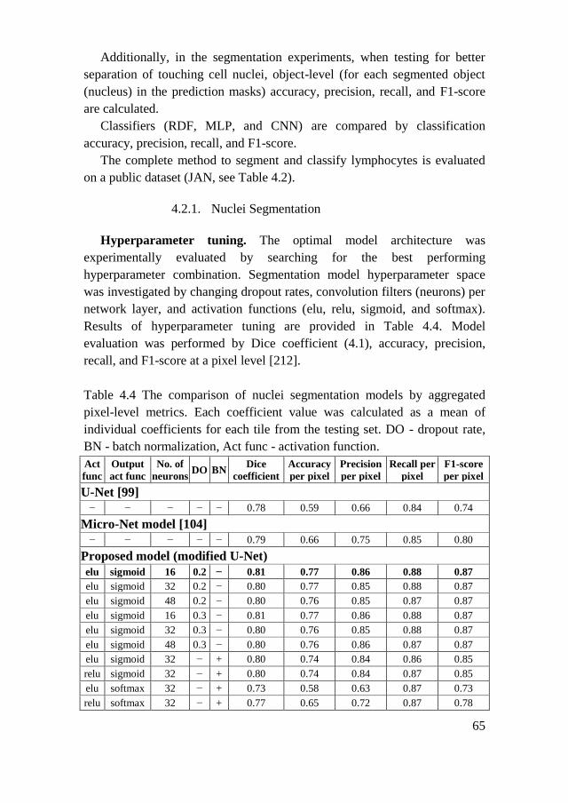
65
Additionally, in the segmentation experiments, when testing for better
separation of touching cell nuclei, object-level (for each segmented object
(nucleus) in the prediction masks) accuracy, precision, recall, and F1-score
are calculated.
Classifiers (RDF, MLP, and CNN) are compared by classification
accuracy, precision, recall, and F1-score.
The complete method to segment and classify lymphocytes is evaluated
on a public dataset (JAN, see Table 4.2).
4.2.1. Nuclei Segmentation
Hyperparameter tuning. The optimal model architecture was
experimentally evaluated by searching for the best performing
hyperparameter combination. Segmentation model hyperparameter space
was investigated by changing dropout rates, convolution filters (neurons) per
network layer, and activation functions (elu, relu, sigmoid, and softmax).
Results of hyperparameter tuning are provided in Table 4.4. Model
evaluation was performed by Dice coefficient (4.1), accuracy, precision,
recall, and F1-score at a pixel level [212].
Table 4.4 The comparison of nuclei segmentation models by aggregated
pixel-level metrics. Each coefficient value was calculated as a mean of
individual coefficients for each tile from the testing set. DO - dropout rate,
BN - batch normalization, Act func - activation function.
Act
func
Output
act func
No. of
neurons DO BN
Dice
coefficient
Accuracy
per pixel
Precision
per pixel
Recall per
pixel
F1-score
per pixel
U-Net [99]
− − − − − 0.78 0.59 0.66 0.84 0.74
Micro-Net model [104]
− − − − − 0.79 0.66 0.75 0.85 0.80
Proposed model (modified U-Net)
elu sigmoid 16 0.2 − 0.81 0.77 0.86 0.88 0.87
elu sigmoid 32 0.2 − 0.80 0.77 0.85 0.88 0.87
elu sigmoid 48 0.2 − 0.80 0.76 0.85 0.87 0.87
elu sigmoid 16 0.3 − 0.81 0.77 0.86 0.88 0.87
elu sigmoid 32 0.3 − 0.80 0.76 0.85 0.88 0.87
elu sigmoid 48 0.3 − 0.80 0.76 0.86 0.87 0.87
elu sigmoid 32 − + 0.80 0.74 0.84 0.86 0.85
relu sigmoid 32 − + 0.80 0.74 0.84 0.87 0.85
elu softmax 32 − + 0.73 0.58 0.63 0.87 0.73
relu softmax 32 − + 0.77 0.65 0.72 0.87 0.78

66
Experiments indicate that expansion of model layer width (16, 32, 48
neurons per convolutional layer) dramatically did not affect the segmentation
performance metrics – which suggests that an introduced texture block
component may ensure consistent feature extraction in a wide range of
model width. Compared to the U-Net model, which reached 0.78 Dice
coefficient for the testing dataset, the selected model achieved 0.81 Dice
coefficient with lower model complexity.
Model performance speed. Optimal model selection rationale was based
on pixel-level testing metrics, and additionally, loading and inference times
relative to the original Micro-Net model were evaluated. Since no significant
changes were observed between dropout rates, the dropout rate was set to
0.2, and an elu activation and sigmoid output functions with differing layer
widths of 16, 32, and 48 kernels were selected. The testing results provided
in Table 4.5 indicate that the lowest relative image prediction and model
loading time was observed for the segmentation model consisting of 16
neurons per convolutional layer.
Table 4.5 A comparison table of loading and inference speeds of modified
U-Net model versions. All times were obtained relative to the original
Micro-Net model. The best-performing model is highlighted in bold.
Model Relative loading time Relative inference time
Micro-Net 1 1
Custom-16 0.212 0.288
Custom-32 0.212 0.314
Custom-48 0.268 0.359
Active contour layer. To evaluate the impact of the active contour layer
on nuclei separation, a modified U-Net was trained using single-layered
nuclei masks and compared the results with an identical model trained on
two-layered annotations. During this experiment, the best-scoring model
architecture from the hyperparameter search experiment was used.
To reveal the effect of training for nuclei contours on clumped object
separation, both pixel-level and object-level metrics were employed. The
Dice coefficient (4.1) was used to track pixel-level segmentation
performance, while object-level segmentation quality was evaluated by
calculating intersection over union (IoU), see Equation 4.4 [212, 213].
𝐼𝑜𝑈 = 𝑇𝑃
𝐹𝑃+𝑇𝑃+𝐹𝑁 (4.4)
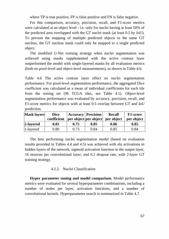
67
where TP is true positive, FP is false positive and FN is false negative.
For this comparison, accuracy, precision, recall, and F1-score metrics
were calculated at an object level - i.e. only for nuclei having at least 50% of
the predicted area overlapped with the GT nuclei mask (at least 0.5 by IoU).
To prevent the mapping of multiple predicted objects to the same GT
nucleus, the GT nucleus mask could only be mapped to a single predicted
object.
The modified U-Net training strategy when nuclei segmentation was
achieved using masks supplemented with the active contour layer
outperformed the model with single-layered masks by all evaluation metrics
(both on pixel-level and object-level measurements), as shown in Table 4.6.
Table 4.6 The active contour layer effect on nuclei segmentation
performance. For pixel-level segmentation performance, the aggregated Dice
coefficient was calculated as a mean of individual coefficients for each tile
from the testing set (96 TCGA tiles, see Table 4.1). Object-level
segmentation performance was evaluated by accuracy, precision, recall, and
F1-score metrics for objects with at least 0.5 overlap between GT and IoU
prediction.
Mask layers Dice
coefficient
Accuracy
per object
Precision
per object
Recall
per object
F1-score
per object
2-layered 0.81 0.75 0.85 0.86 0.85
1-layered 0.80 0.73 0.84 0.85 0.84
The best performing nuclei segmentation model (based on evaluation
results provided in Tables 4.4 and 4.5) was achieved with elu activations in
hidden layers of the network, sigmoid activation function in the output layer,
16 neurons per convolutional layer, and 0.2 dropout rate, with 2-layer GT
training strategy.
4.2.2. Nuclei Classification
Hyper parameter tuning and model comparison. Model performance
metrics were evaluated for several hyperparameter combinations, including a
number of nodes per layer, activation functions, and a number of
convolutional kernels. Hyperparameter search is summarized in Table 4.7.
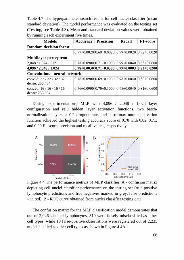
68
Table 4.7 The hyperparameter search results for cell nuclei classifier (mean
standard deviation). The model performance was evaluated on the testing set
(Testing, see Table 4.3). Mean and standard deviation values were obtained
by running each experiment five times.
Models Accuracy Precision Recall F1-score
Random decision forest
0.77±0.0020 0.69±0.0020 0.99±0.0020 0.82±0.0020
Multilayer perceptron
2,048 / 1,024 / 512 0.78±0.0900 0.71±0.1000 0.99±0.0040 0.83±0.0600
4,096 / 2,048 / 1,024 0.78±0.0030 0.71±0.0300 0.99±0.0003 0.82±0.0200
Convolutional neural network
conv2d: 32 / 32 / 32 / 32
dense: 256 / 64
0.76±0.0900 0.69±0.1000 0.98±0.0040 0.80±0.0600
conv2d: 16 / 16 / 16 / 16
dense: 256 / 64
0.76±0.0900 0.70±0.1000 0.98±0.0040 0.81±0.0600
During experimentations, MLP with 4,096 / 2,048 / 1,024 layer
configuration and relu hidden layer activation functions, two batch-
normalization layers, a 0.2 dropout rate, and a softmax output activation
function achieved the highest testing accuracy score of 0.78 with 0.82, 0.71,
and 0.99 F1-score, precision and recall values, respectively.
Figure 4.4 The performance metrics of MLP classifier. A - confusion matrix
depicting cell nuclei classifier performance on the testing set (true positive
lymphocyte predictions and true negatives marked in grey, false predictions
– in red), B - ROC curve obtained from nuclei classifier testing data.
The confusion matrix for the MLP classification model demonstrates that
out of 2,046 labelled lymphocytes, 310 were falsely misclassified as other
cell types, while 13 false-positive observations were registered out of 2,235
nuclei labelled as other cell types as shown in Figure 4.4A.
A B
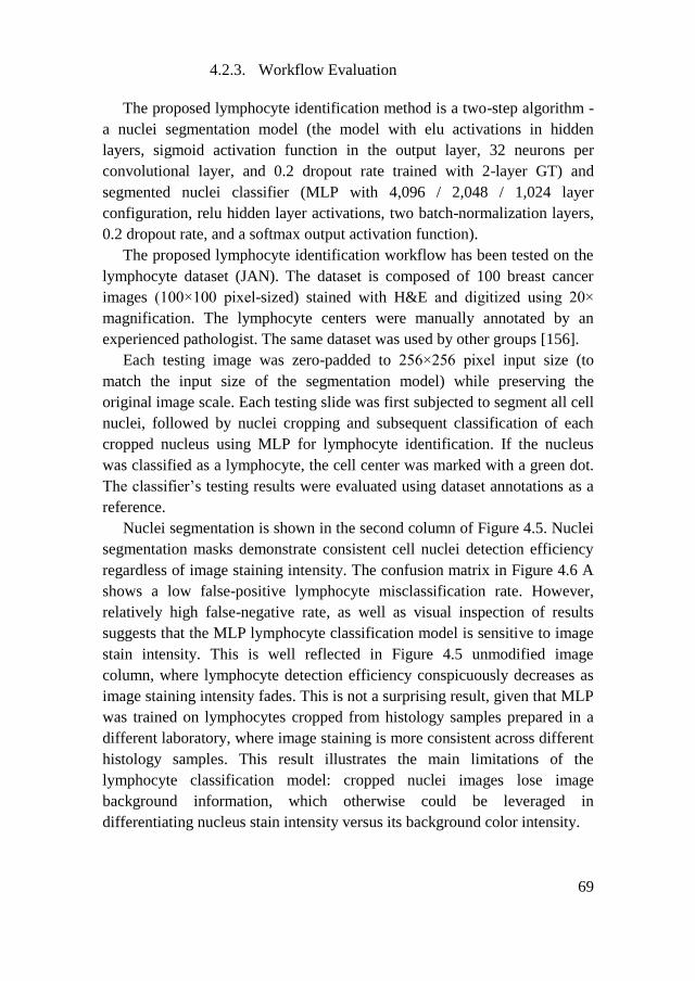
69
4.2.3. Workflow Evaluation
The proposed lymphocyte identification method is a two-step algorithm -
a nuclei segmentation model (the model with elu activations in hidden
layers, sigmoid activation function in the output layer, 32 neurons per
convolutional layer, and 0.2 dropout rate trained with 2-layer GT) and
segmented nuclei classifier (MLP with 4,096 / 2,048 / 1,024 layer
configuration, relu hidden layer activations, two batch-normalization layers,
0.2 dropout rate, and a softmax output activation function).
The proposed lymphocyte identification workflow has been tested on the
lymphocyte dataset (JAN). The dataset is composed of 100 breast cancer
images (100×100 pixel-sized) stained with H&E and digitized using 20×
magnification. The lymphocyte centers were manually annotated by an
experienced pathologist. The same dataset was used by other groups [156].
Each testing image was zero-padded to 256×256 pixel input size (to
match the input size of the segmentation model) while preserving the
original image scale. Each testing slide was first subjected to segment all cell
nuclei, followed by nuclei cropping and subsequent classification of each
cropped nucleus using MLP for lymphocyte identification. If the nucleus
was classified as a lymphocyte, the cell center was marked with a green dot.
The classifier’s testing results were evaluated using dataset annotations as a
reference.
Nuclei segmentation is shown in the second column of Figure 4.5. Nuclei
segmentation masks demonstrate consistent cell nuclei detection efficiency
regardless of image staining intensity. The confusion matrix in Figure 4.6 A
shows a low false-positive lymphocyte misclassification rate. However,
relatively high false-negative rate, as well as visual inspection of results
suggests that the MLP lymphocyte classification model is sensitive to image
stain intensity. This is well reflected in Figure 4.5 unmodified image
column, where lymphocyte detection efficiency conspicuously decreases as
image staining intensity fades. This is not a surprising result, given that MLP
was trained on lymphocytes cropped from histology samples prepared in a
different laboratory, where image staining is more consistent across different
histology samples. This result illustrates the main limitations of the
lymphocyte classification model: cropped nuclei images lose image
background information, which otherwise could be leveraged in
differentiating nucleus stain intensity versus its background color intensity.

70
Figure 4.5 Examples of 5 testing images from breast cancer lymphocyte
dataset (JAN) with corresponding lymphocyte identification model outputs.
From left to right: 1st column- original testing image from the lymphocyte
dataset. 2nd column: nuclei segmentation predictions by the modified Micro-
Net. 3rd column: expert pathologist’s annotation (marked lymphocyte
centers) supplied in the dataset. 4th column: MLP lymphocyte classifier
result (if the nucleus was predicted as a lymphocyte, its center was labelled
with a green dot). 5th column: lymphocyte classifier results after the
Reinhard [214] stain normalization.
The effect of color normalization on overall model performance. To
address high staining variability between different histological samples, the
lymphocyte testing dataset was normalized using the Reinhard stain
normalization method. The Reinhard algorithm adjusts the source image’s
color distribution to the color distribution of the target image by equalizing
the mean and standard deviation pixel values in each channel [214].
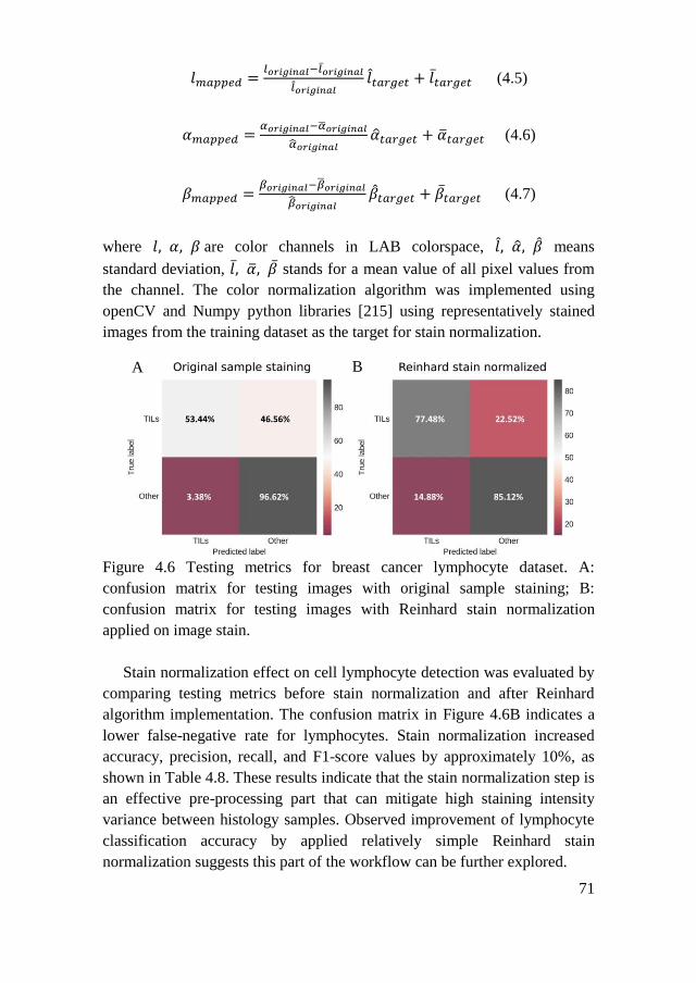
71
𝑙𝑚𝑎𝑝𝑝𝑒𝑑 =𝑙𝑜𝑟𝑖𝑔𝑖𝑛𝑎𝑙−𝑙�̅�𝑟𝑖𝑔𝑖𝑛𝑎𝑙
𝑙𝑜𝑟𝑖𝑔𝑖𝑛𝑎𝑙𝑙𝑡𝑎𝑟𝑔𝑒𝑡 + 𝑙�̅�𝑎𝑟𝑔𝑒𝑡 (4.5)
𝛼𝑚𝑎𝑝𝑝𝑒𝑑 =𝛼𝑜𝑟𝑖𝑔𝑖𝑛𝑎𝑙−�̅�𝑜𝑟𝑖𝑔𝑖𝑛𝑎𝑙
�̂�𝑜𝑟𝑖𝑔𝑖𝑛𝑎𝑙�̂�𝑡𝑎𝑟𝑔𝑒𝑡 + �̅�𝑡𝑎𝑟𝑔𝑒𝑡 (4.6)
𝛽𝑚𝑎𝑝𝑝𝑒𝑑 =𝛽𝑜𝑟𝑖𝑔𝑖𝑛𝑎𝑙−�̅�𝑜𝑟𝑖𝑔𝑖𝑛𝑎𝑙
�̂�𝑜𝑟𝑖𝑔𝑖𝑛𝑎𝑙�̂�𝑡𝑎𝑟𝑔𝑒𝑡 + �̅�𝑡𝑎𝑟𝑔𝑒𝑡 (4.7)
where 𝑙, 𝛼, 𝛽are color channels in LAB colorspace, 𝑙, �̂�, �̂� means
standard deviation, 𝑙,̅ �̅�, �̅� stands for a mean value of all pixel values from
the channel. The color normalization algorithm was implemented using
openCV and Numpy python libraries [215] using representatively stained
images from the training dataset as the target for stain normalization.
Figure 4.6 Testing metrics for breast cancer lymphocyte dataset. A:
confusion matrix for testing images with original sample staining; B:
confusion matrix for testing images with Reinhard stain normalization
applied on image stain.
Stain normalization effect on cell lymphocyte detection was evaluated by
comparing testing metrics before stain normalization and after Reinhard
algorithm implementation. The confusion matrix in Figure 4.6B indicates a
lower false-negative rate for lymphocytes. Stain normalization increased
accuracy, precision, recall, and F1-score values by approximately 10%, as
shown in Table 4.8. These results indicate that the stain normalization step is
an effective pre-processing part that can mitigate high staining intensity
variance between histology samples. Observed improvement of lymphocyte
classification accuracy by applied relatively simple Reinhard stain
normalization suggests this part of the workflow can be further explored.
A B
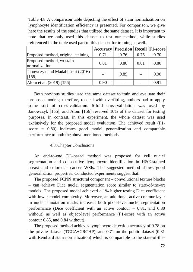
72
Table 4.8 A comparison table depicting the effect of stain normalization on
lymphocyte identification efficiency is presented. For comparison, we give
here the results of the studies that utilized the same dataset. It is important to
note that we only used this dataset to test our method, while studies
referenced in the table used part of this dataset for training as well.
Accuracy Precision Recall F1-score
Proposed method, original staining 0.71 0.76 0.75 0.70
Proposed method, wt stain
normalization 0.81 0.80 0.81 0.80
Janowczyk and Madabhushi (2016)
[155] – 0.89 – 0.90
Alom et al. (2019) [156] 0.90 – – 0.91
Both previous studies used the same dataset to train and evaluate their
proposed models; therefore, to deal with overfitting, authors had to apply
some sort of cross-validation. 5-fold cross-validation was used by
Janowczyk [155], and Alom [156] reserved 10% of the dataset for testing
purposes. In contrast, in this experiment, the whole dataset was used
exclusively for the proposed model evaluation. The achieved result (F1-
score = 0.80) indicates good model generalization and comparable
performance to both the above-mentioned methods.
4.3. Chapter Conclusions
An end-to-end DL-based method was proposed for cell nuclei
segmentation and consecutive lymphocyte identification in H&E-stained
breast and colorectal cancer WSIs. The suggested method shows good
generalization properties. Conducted experiments suggest that:
The proposed FCNN structural component – convolutional texture blocks
– can achieve Dice nuclei segmentation score similar to state-of-the-art
models. The proposed model achieved a 1% higher testing Dice coefficient
with lower model complexity. Moreover, an additional active contour layer
in nuclei annotation masks increases both pixel-level nuclei segmentation
performance (Dice coefficient with an active contour – 0.81, and 0.80
without) as well as object-level performance (F1-score with an active
contour 0.85, and 0.84 without).
The proposed method achieves lymphocyte detection accuracy of 0.78 on
the private dataset (TCGA+CRCHP), and 0.71 on the public dataset (0.81
with Reinhard stain normalization) which is comparable to the state-of-the-
73
art lymphocyte detection methods. The achieved result indicates good model
generalization properties by providing lymphocyte segmentation capability
as well.
74
5. COLLAGEN FRAMEWORK SEGMENTATION
This chapter explores the segmentation of collagen fibers from routine
bright-field histology images of breast tumor tissue by an FCNN-based
model. Collagen is the third TME compartment addressed in this thesis.
Being a fundamental component of TME with massive potential in solid
tumor diagnostics (as discussed in Chapter 2.2.3) collagen lacks assessment
methods that would not heavily rely on specialized and expensive imaging
techniques to the best of our knowledge. This fact inspires and motivates the
development of a robust and affordable method for assessing biological
information of collagen architecture from readily available bright-field
microscopy images (routinely used in diagnostic pathology laboratories all
over the world). Due to its complex structure and the abundance in the
connective tissue, fibrous collagen is quite challenging to annotate by
outlining manually. It is even complicated to define collagen as a target for
segmentation tasks. Therefore this experiment utilizes another commonly
used pathologic tissue staining method - Sirius Red (SR) to highlight
collagen in breast tumor tissues. The knowledge gained in this experiment
will be applied in Chapter 6 to further explore and test collagen
segmentation on routine H&E-stained tumor tissue WSIs.
5.1. Experiment Design
The first task addressed in this chapter is the generation of ground truth
for collagen segmentation. A set of 116 non-overlapping 256×256 pixel-
sized image patches is randomly generated from 48 tumor images and
subjected to expert annotation. GT is obtained from three different sources
(fully manual and semi-automated). Human visual bias is revealed by Bland-
Altman difference analysis [216, 217], and the consensual information in
acquired GT is captured by the histogram of oriented gradients (HOG [218]).
To address the collagen segmentation task, U-Net is chosen as a base
model. The fibrous tissue collagen structure forms distinctive textural
patterns; therefore, to better capture mesh-like collagen, the U-Net
architecture is modified by introducing the texture block (described in
Chapter 4.1.2, also see Figure 4.2). Three models are trained on annotated
image patches to segment collagen fibers in the entire collection of 92
tumorous tissue images. The effect of different model training modes on
segmentation accuracy is evaluated by intersection, coverage, and ratio
analysis [209]). Subsequently, features of collagen fiber morphometry,
75
density, orientation, texture, and fractal characteristics are defined and
extracted from collagen segmentation maps (CSM). To gain an
understanding of the general properties of collagen framework architecture,
factor analysis [196] is performed.
Univariate prognostic modeling (Kaplan-Meier estimates [219]) is
applied to reveal collagen fiber features indicative of patient prognosis. One-
way ANOVA and Tukey’s HSD post hoc test [220] are employed to uncover
significant associations between collagen fiber features and tumor histology
groups.
Finally, prognostic models for collagen fiber features (derived by each
differently trained FCNN model) are obtained in multivariate Cox regression
analysis [221], and significant and independent collagen features are
identified as prognostic indicators.
5.1.1. Datasets
Patients. The Lithuanian Bioethics Committee approved this study
(reference number: 40, date 2007-04-26, updated 2017-09-12).
Two hundred three patients involved in this and previous studies [175,
176] underwent surgery during 2007-2009 at the National Cancer Institute
(Lithuania, Vilnius). During this period, tumor samples were collected
prospectively, and the pathologist’s examination of these samples was
performed at the National Centre of Pathology (Lithuania, Vilnius). One
hundred seven patients were diagnosed with an early-stage hormone
receptor-positive invasive ductal breast carcinoma.
Samples. Tumor tissue samples from 92 patients were used for the
analyses. Clinicopathological characteristics and follow-up data from these
patients are reported as the mean and median values for continuous variables
and the frequencies of categorical variables and are given in Table 5.1.
Patients in this group were females at the age of 27 to 87 years followed for
a period of 17 to 121 months after surgery. Hormone receptor positivity was
defined previously [176] as estrogen receptor or progesterone receptor
immunohistochemical positivity in at least 1% of tumor cells.

76
Figure 5.1 Tissue microarray (TMA) samples (each TMA spot has a 1mm
diameter).
Table 5.1 Characteristics of patients with hormone receptor-positive breast
carcinoma.
Clinicopathological parameters Patients (%)
Total 92 (100%)
Age, years
Mean 57.27
Median 59
Range 27-87
Gender
Female 92 (100%)
Male 0 (0%)
Histological grade (G)
G1 19 (20.65%)
G2 44 (47.83%)
G3 29 (31.52%)
Tumor invasion stage (T)
T1 52 (56.52%)
T2 40 (43.48%)
T3 0 (0%)
T4 0 (0%)
Lymph node metastasis status (N)
N0 48 (51.17%)
N1 30 (32.61%)
N2 11 (11.83%)
N3 3 (3.26%)
Intrinsic subtype
Luminal A 49 (53.26%)
Luminal B, HER2 negative 26 (28.26%)
Luminal B, HER2 possitive 17 (18.48%)
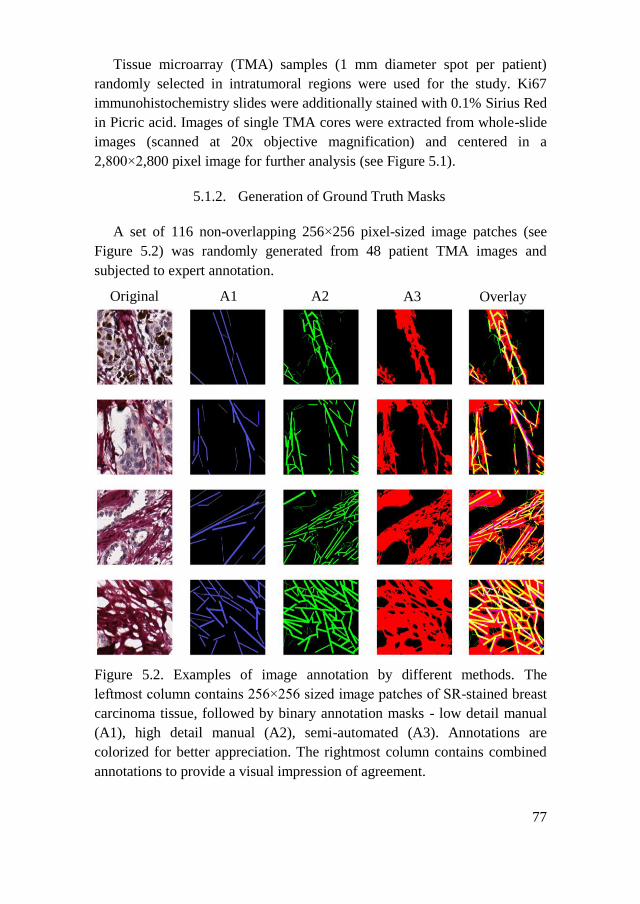
77
Tissue microarray (TMA) samples (1 mm diameter spot per patient)
randomly selected in intratumoral regions were used for the study. Ki67
immunohistochemistry slides were additionally stained with 0.1% Sirius Red
in Picric acid. Images of single TMA cores were extracted from whole-slide
images (scanned at 20x objective magnification) and centered in a
2,800×2,800 pixel image for further analysis (see Figure 5.1).
5.1.2. Generation of Ground Truth Masks
A set of 116 non-overlapping 256×256 pixel-sized image patches (see
Figure 5.2) was randomly generated from 48 patient TMA images and
subjected to expert annotation.
Figure 5.2. Examples of image annotation by different methods. The
leftmost column contains 256×256 sized image patches of SR-stained breast
carcinoma tissue, followed by binary annotation masks - low detail manual
(A1), high detail manual (A2), semi-automated (A3). Annotations are
colorized for better appreciation. The rightmost column contains combined
annotations to provide a visual impression of agreement.
Original A1 Overlay A3 A2
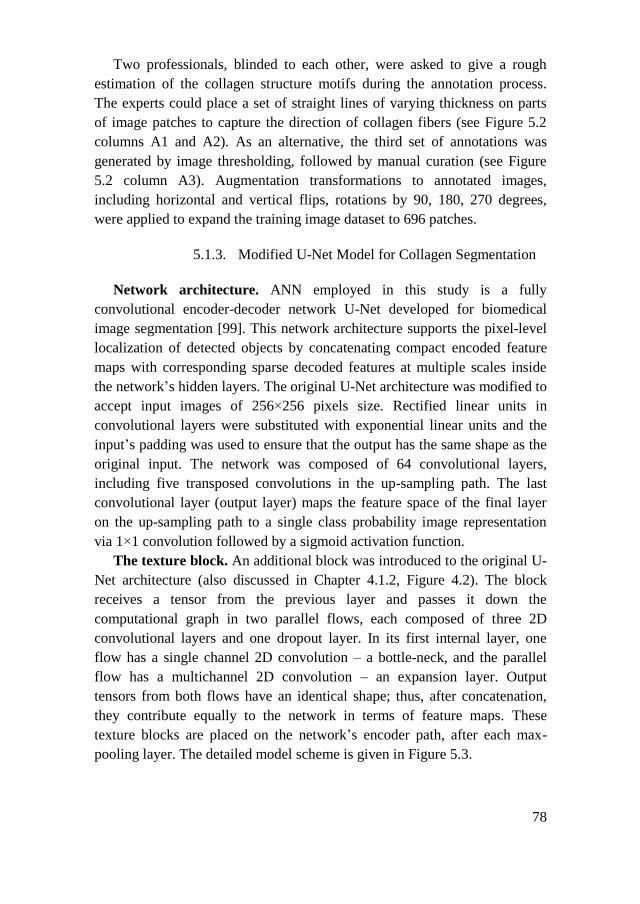
78
Two professionals, blinded to each other, were asked to give a rough
estimation of the collagen structure motifs during the annotation process.
The experts could place a set of straight lines of varying thickness on parts
of image patches to capture the direction of collagen fibers (see Figure 5.2
columns A1 and A2). As an alternative, the third set of annotations was
generated by image thresholding, followed by manual curation (see Figure
5.2 column A3). Augmentation transformations to annotated images,
including horizontal and vertical flips, rotations by 90, 180, 270 degrees,
were applied to expand the training image dataset to 696 patches.
5.1.3. Modified U-Net Model for Collagen Segmentation
Network architecture. ANN employed in this study is a fully
convolutional encoder-decoder network U-Net developed for biomedical
image segmentation [99]. This network architecture supports the pixel-level
localization of detected objects by concatenating compact encoded feature
maps with corresponding sparse decoded features at multiple scales inside
the network’s hidden layers. The original U-Net architecture was modified to
accept input images of 256×256 pixels size. Rectified linear units in
convolutional layers were substituted with exponential linear units and the
input’s padding was used to ensure that the output has the same shape as the
original input. The network was composed of 64 convolutional layers,
including five transposed convolutions in the up-sampling path. The last
convolutional layer (output layer) maps the feature space of the final layer
on the up-sampling path to a single class probability image representation
via 1×1 convolution followed by a sigmoid activation function.
The texture block. An additional block was introduced to the original U-
Net architecture (also discussed in Chapter 4.1.2, Figure 4.2). The block
receives a tensor from the previous layer and passes it down the
computational graph in two parallel flows, each composed of three 2D
convolutional layers and one dropout layer. In its first internal layer, one
flow has a single channel 2D convolution – a bottle-neck, and the parallel
flow has a multichannel 2D convolution – an expansion layer. Output
tensors from both flows have an identical shape; thus, after concatenation,
they contribute equally to the network in terms of feature maps. These
texture blocks are placed on the network’s encoder path, after each max-
pooling layer. The detailed model scheme is given in Figure 5.3.
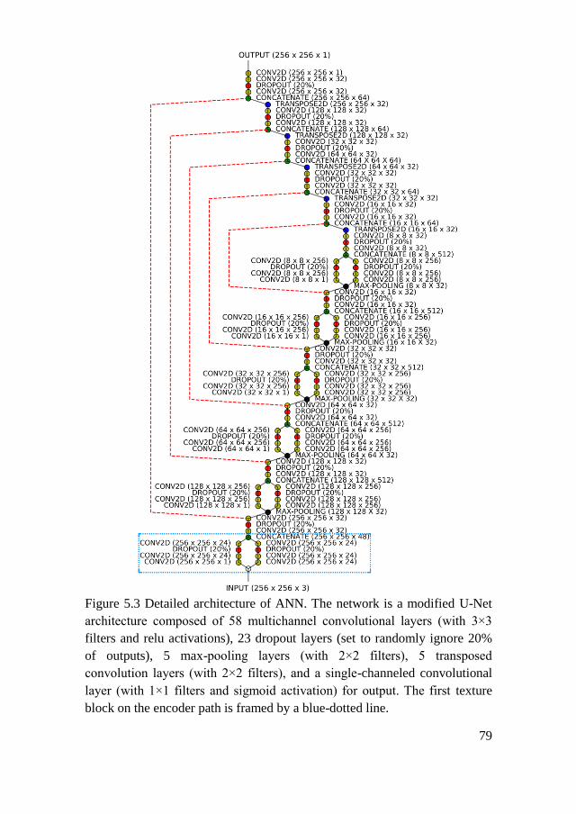
79
Figure 5.3 Detailed architecture of ANN. The network is a modified U-Net
architecture composed of 58 multichannel convolutional layers (with 3×3
filters and relu activations), 23 dropout layers (set to randomly ignore 20%
of outputs), 5 max-pooling layers (with 2×2 filters), 5 transposed
convolution layers (with 2×2 filters), and a single-channeled convolutional
layer (with 1×1 filters and sigmoid activation) for output. The first texture
block on the encoder path is framed by a blue-dotted line.
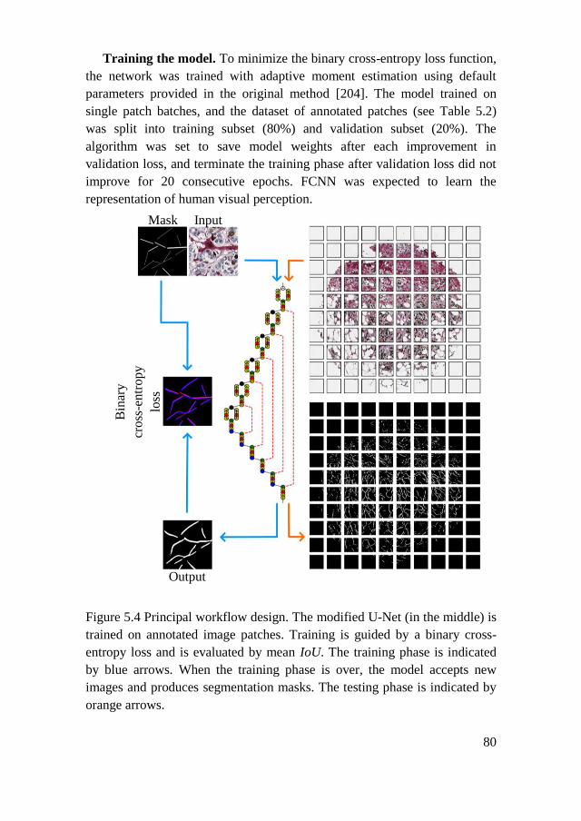
80
Training the model. To minimize the binary cross-entropy loss function,
the network was trained with adaptive moment estimation using default
parameters provided in the original method [204]. The model trained on
single patch batches, and the dataset of annotated patches (see Table 5.2)
was split into training subset (80%) and validation subset (20%). The
algorithm was set to save model weights after each improvement in
validation loss, and terminate the training phase after validation loss did not
improve for 20 consecutive epochs. FCNN was expected to learn the
representation of human visual perception.
Figure 5.4 Principal workflow design. The modified U-Net (in the middle) is
trained on annotated image patches. Training is guided by a binary cross-
entropy loss and is evaluated by mean IoU. The training phase is indicated
by blue arrows. When the training phase is over, the model accepts new
images and produces segmentation masks. The testing phase is indicated by
orange arrows.
Output
Bin
ary
cross
-entr
opy
loss
Mask Input

81
Table 5.2 Three collagen segmentation models were trained on sets of
different expert-provided annotations.
Model Training images
(256×256 pixel size)
Ground truth
(256×256 pixel size)
M1 696 augmented (flip, rotation)
image patches (see Figure 5.2
Original)
556 patches used for training
140 patches used for validation
696 low detail manual annotation
masks (see Figure 5.2 A1)
M2 696 high detail manual annotation
masks (see Figure 5.2 A2)
M3 696 semi-automated annotation
masks (see Figure 5.2 A3)
Principle of collagen framework detection by a neural network. An
overview of the workflow is given in Figure 5.4. To fit the model input
shape, the TMA image is split into overlapping (128-pixel step-size in
vertical and horizontal directions on an image plane) 256×256 pixel size
patches. The trained model performs predictions patch-by-patch to produce
probability maps that, in turn, are subjected to thresholding. Each pixel in a
probability map receives a value of 1.0 if the probability of detecting
collagen in that pixel is higher than 0.5. Otherwise, the pixel receives a value
of 0.0
To avoid prediction artifacts at patch borders, predictions were taken into
account only when present in both overlapping resulting patch analysis
probability maps. The results were merged to form a binary collagen
segmentation mask (CSM) of an original image of a single TMA spot.
Lastly, the size filtering of detected objects was applied removing objects
containing less than 50 pixels.
Model evaluation. During the training phase, model progress was
monitored by prediction-annotation similarity. An intersection over union
(IoU, see equation 4.4) metrics was employed.
For pairwise comparison of CSMs produced by different ANN models,
similarity was aggregated as a mean ratio of non-zero pixel counts between
CSMs, mean coverage, and mean IoU of all analyzed CSMs:
𝑚𝑒𝑎𝑛𝑟𝑎𝑡𝑖𝑜 =1
𝑁∑
𝐶𝑆𝑀𝑖,𝑚𝑜𝑑1
𝐶𝑆𝑀𝑖,𝑚𝑜𝑑2
𝑁
𝑖=1
,
𝑚𝑒𝑎𝑛_𝑐𝑜𝑣𝑒𝑟𝑎𝑔𝑒 =1
𝑁∑
𝐶𝑆𝑀𝑖,𝑚𝑜𝑑1⋂𝐶𝑆𝑀𝑖,𝑚𝑜𝑑2
𝐶𝑆𝑀𝑖,𝑚𝑜𝑑1 ,
𝑁
𝑖=1
82
𝑚𝑒𝑎𝑛_𝐼𝑜𝑈 =1
𝑁∑
𝐶𝑆𝑀𝑖,𝑚𝑜𝑑1⋂𝐶𝑆𝑀𝑖,𝑚𝑜𝑑2
𝐶𝑆𝑀𝑖,𝑚𝑜𝑑1⋃𝐶𝑆𝑀𝑖,𝑚𝑜𝑑2
𝑁
𝑖=1
where 𝑁 is the number of images compared, and 𝑚𝑜𝑑𝑖 is an individually
trained modified U-Net model.
Since no GT was available at a full image level, visual estimation of
consensual information in segmentation masks resulting from different
models was considered.
5.1.4. Collagen Fiber Morphometry
Quantitative feature extraction. The collagen fibers were analyzed by
computing 37 features that fall into three major groups: pixel-level features
such as angle and magnitude of the orientation of edges present in an area
surrounding a pixel in CSM; fiber-level features include morphometric
measures of each detected object (individual collagen fiber); image-level
features such as fractal characteristics and texture descriptors of the pixel-
level feature representation images. Since the study used a single TMA core
image per patient, all image-level features also represent the single patient.
Fiber-level and pixel-level features were extracted and aggregated by the
mean, median, or standard deviation for each patient (see Table 5.3).
Pixel-level features. Fiber orientation features for each pixel in the target
image were measured by a histogram of oriented gradients (HOG [218]). A
bounding box (context area) of 18×18 pixels size for a pixel of interest was
selected by calibration. Unsigned gradients (originating from edges present
in an image) were summarized in 64 evenly spread histogram bins covering
a range of 0 – 180 degree angles. A Sobel operator [222] was used in both x
and y directions in an image plane to estimate gradients present in an image.
HOG procedure then counts occurrences of gradient orientation in image
patches and assigns the gradient magnitude of each pixel to the
corresponding histogram bin covering a particular angle. Collagen
framework orientation angle descriptors were summarized by the linear
directional mean, circular variance, and circular standard deviation from the
histogram. Since the fiber orientation angle is dependent upon tissue
placement on the glass slide, the only meaningful fiber orientation angle
related feature at the image level was the circular standard deviation (CSD,
see Table 5.3). The magnitude of gradients was summarized by the mean
and standard deviation (for histogram values where magnitude was not zero).
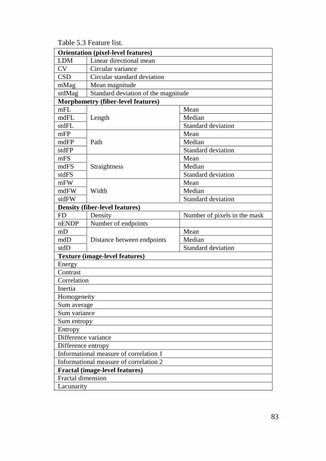
83
Table 5.3 Feature list.
Orientation (pixel-level features)
LDM Linear directional mean
CV Circular variance
CSD Circular standard deviation
mMag Mean magnitude
stdMag Standard deviation of the magnitude
Morphometry (fiber-level features)
mFL
Length
Mean
mdFL Median
stdFL Standard deviation
mFP
Path
Mean
mdFP Median
stdFP Standard deviation
mFS
Straightness
Mean
mdFS Median
stdFS Standard deviation
mFW
Width
Mean
mdFW Median
stdFW Standard deviation
Density (fiber-level features)
FD Density Number of pixels in the mask
nENDP Number of endpoints
mD
Distance between endpoints
Mean
mdD Median
stdD Standard deviation
Texture (image-level features)
Energy
Contrast
Correlation
Inertia
Homogeneity
Sum average
Sum variance
Sum entropy
Entropy
Difference variance
Difference entropy
Informational measure of correlation 1
Informational measure of correlation 2
Fractal (image-level features)
Fractal dimension
Lacunarity

84
Fiber-level features. Morphometric features of collagen fibers were
computed treating each fiber as a separate object and subsequently
aggregated for each patient by mean values. Fiber objects were bound in a
minimum bounding rectangle, and a diagonal of this rectangle was used as a
fiber length (FL) measure. The length of a fiber centerline, or the fiber path
(FP - defined as a line that divides a fiber into two equal parts along its
longer axis), was calculated as half of the total number of points in a fiber
contour. The fiber width (FW) was computed as half the Euclidean distance
between all opposing pairs of points in the fiber contour aggregated by the
median. Fiber straightness (FS) was calculated as a ratio of FL over FP.
Fiber density (FD) was computed as a mean Euclidean distance from each
detected fiber endpoint to all neighbor endpoints in CSM.
Image-level features. Fractal characteristics and texture features of the
collagen framework were computed from CSMs. Box counting procedure
[223] was employed to compute the fractal dimension and the lacunarity.
The spatial gray-level co-occurrence matrix calculated with a 1px
displacement vector was used to derive image texture descriptors [58],
including energy, contrast, homogeneity, and entropy. To extract texture
descriptors Python computer vision and image processing library Mahotas
[195] was used.
Statistical analysis. The consistency of expert annotations was evaluated
by Bland-Altman difference analysis [216], a one-sample t-test on
differences against the zero value, and an independent sample t-test on cases
in a 95% agreement interval. In an exploratory analysis, Shapiro–Wilk and
Levene’s tests were used for data normality and homogeneity assumptions.
One-way ANOVA and Tukey’s HSD post hoc tests [220] were employed to
assess differences between group means. FA was performed as described in
[196] - with the principal component method using a covariance matrix of
Pearson’s correlations of the variables. Varimax rotation was applied to
simplify the structure of factors and improve the interpretation. Cutoff points
for variables were determined, and patients were stratified into groups based
on statistical differences as assessed by a log-rank test. Kaplan-Meier
estimates [219] were used to assess patient survival. Feature validation was
performed following a leave-one-out strategy, as described previously [224].
Cox proportional hazards analysis [221] was applied to model the effect of
multiple variables on patients’ survival time. For all tests to prove the
significance a p-value <0.05 was accepted.

85
Implementation. For DL TensorFlow framework in Python was used
[198]. Full training (training from scratch) of the model was performed on a
high-performance graphical processing unit (Nvidia GeForce GTX1080).
Feature extraction and quantification were implemented using the scikit-
image image processing library in Python [225].
All statistical analyses were performed in the R statistical environment.
The Cutoff Finder algorithm [226] was applied for univariate survival
analysis and a survival package [227] for multivariate statistical modeling.
5.2. Results
Expert annotation consistency. Regions containing fibrous collagen can
be appreciated visually in SR-stained bright-field microscopy images; also,
the histogram of oriented gradients procedure enables reliable detection of
the fiber orientation (see Figure 5.5).
Figure 5.5 Annotation consistency. (A) SR stained breast carcinoma tissue.
256×256 pixel-sized excerpt from original image. (B) binary annotation
mask produced by a semi-automated method. (C and D) binary annotation
masks (of the same image patch) produced manually. (E, F, G, H) polar
projections of histograms of orientations captured by HOG procedure from
corresponding (A, B, C, D) images. Note that all annotations differ by the
level of detail but basically agree on orientation.
The consistency of the collagen framework annotation procedure was
evaluated by Bland-Altman difference analysis [216, 217] of the two
“manual” approaches focusing on differences in the count of annotated
objects, average object size (in pixels), and the dominant orientation of
annotated objects (in degrees).
H
A
E F G H
B C D

86
Table 5.4 Annotation consistency between experts
Parameters of annotated objects
Count Size Orientation
Mean difference -25.303 151.485 2.184
One-sample t-statistics -13.860 5.718 2.052
p-value 7.914×10⁻²⁵ 1.170×10⁻⁷ 0.043
95% limits of agreement ± 35.423 ± 514.076 ± 20.652
Independent sample t-
statistics
-13.603 6.897 0.4851
p-value 1.059×10⁻²⁹ 7.641×10⁻¹¹ 0.628
The analysis revealed significant differences in the level of detail the
experts put into their annotations, as well as the orientation of marked
objects. The one-sample t-test on differences against the zero value shows
the presence of fixed bias for all parameters evaluated (p-value >0.05 for all
estimates). However, in the 95% agreement interval, the differences in
annotation orientations are not significant (p-value = 0.628, see Table 5.4).
Figure 5.6 Annotation dilation. A different amount of morphological image
dilation was applied to annotation masks using a 5×5 elliptic structuring
element (number of dilation iterations nits = 1, 2, 3). On the left, nondilated
annotations are colored in yellow and every additional dilation iteration gets
a different color.
Model prediction consistency. Before training, different morphological
image dilation amounts were applied to annotated patches using 5×5 square
kernel (number of iterations - nits = 0, 1, 2, 3 see Figure 5.6). The impact of
dilation on model predictions was analyzed by visual comparison as well as
by ratio of areas, intersection and coverage. When raw annotations were
used (nits = 0), models did not produce meaningful results (by visual
assessment), except for M3. Annotation dilation did not affect M3 but
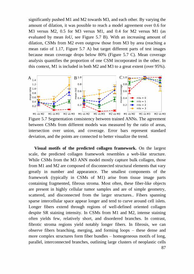
87
significantly pushed M1 and M2 towards M3, and each other. By varying the
amount of dilation, it was possible to reach a model agreement over 0.6 for
M3 versus M2, 0.5 for M3 versus M1, and 0.4 for M2 versus M1 (as
evaluated by mean IoU, see Figure 5.7 B). With an increasing amount of
dilation, CSMs from M2 even outgrow those from M3 by area (reaching a
mean ratio of 1.17, Figure 5.7 A) but target different parts of test images
because mean coverage drops below 80% (Figure 5.7 C). Mean coverage
analysis quantifies the proportion of one CSM incorporated in the other. In
this context, M1 is included in both M2 and M3 to a great extent (over 95%).
Figure 5.7 Segmentation consistency between trained ANNs. The agreement
between CSMs from different models was measured by the ratio of areas,
intersection over union, and coverage. Error bars represent standard
deviation, and the points are connected to better visualize the trend.
Visual motifs of the predicted collagen framework. On the largest
scale, the predicted collagen framework resembles a web-like structure.
While CSMs from the M3 ANN model mostly capture bulk collagen, those
from M1 and M2 are composed of disconnected structural elements that vary
greatly in number and appearance. The smallest components of the
framework (typically in CSMs of M1) arise from tissue image parts
containing fragmented, fibrous stroma. Most often, these fiber-like objects
are present in highly cellular tumor samples and are of simple geometry,
scattered, and disconnected from the larger structures.. Fibers spanning
sparse intercellular space appear longer and tend to curve around cell islets.
Longer fibers extend through regions of well-defined oriented collagen
despite SR staining intensity. In CSMs from M1 and M2, intense staining
often yields few, relatively short, and disordered branches. In contrast,
fibrotic stroma regions yield notably longer fibers. In fibrosis, we can
observe fibers branching, merging, and forming loops – these dense and
more complex structures form fiber bundles – homogeneous motifs of long,
parallel, interconnected branches, outlining large clusters of neoplastic cells
A B
A
C
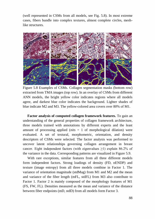
88
(well represented in CSMs from all models, see Fig. 5.8). In most extreme
cases, fibers bundle into complex textures, almost complete circles, mesh-
like structures.
Figure 5.8 Examples of CSMs. Collagen segmentation masks (bottom row)
extracted from TMA images (top row). In an overlay of CSMs from different
ANN models, the bright yellow color indicates regions where all models
agree, and darkest blue color indicates the background. Lighter shades of
blue indicate M2 and M3. The yellow-colored area covers over 80% of M1.
Factor analysis of computed collagen framework features. To gain an
understanding of the general properties of collagen framework architecture,
three models trained with annotations by different experts and the least
amount of processing applied (nits = 1 of morphological dilation) were
evaluated. A set of textural, morphometric, orientation, and density
descriptors of CSMs were selected. The factor analysis was performed to
uncover latent relationships governing collagen arrangement in breast
cancer. Eight independent factors (with eigenvalues ≥1) explain 86.2% of
the variance in the data. Corresponding patterns are visualized in Figure 5.9.
With rare exceptions, similar features from all three different models
form independent factors. Strong loadings of density (FD, nENDP) and
texture (image entropy) from all three models combine in Factor 1. The
variance of orientation magnitude (stdMag) from M1 and M2 and the mean
and variance of the fiber length (mFL, stdFL) from M3 also contribute to
Factor 1. Factor 2 is mainly composed of the morphology features of M1
(FS, FW, FL). Densities measured as the mean and variance of the distance
between fiber endpoints (mD, stdD) from all models form Factor 3.
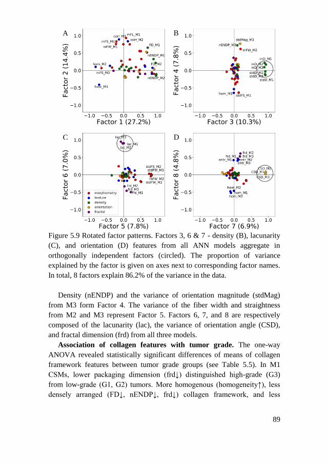
89
Figure 5.9 Rotated factor patterns. Factors 3, 6 & 7 - density (B), lacunarity
(C), and orientation (D) features from all ANN models aggregate in
orthogonally independent factors (circled). The proportion of variance
explained by the factor is given on axes next to corresponding factor names.
In total, 8 factors explain 86.2% of the variance in the data.
Density (nENDP) and the variance of orientation magnitude (stdMag)
from M3 form Factor 4. The variance of the fiber width and straightness
from M2 and M3 represent Factor 5. Factors 6, 7, and 8 are respectively
composed of the lacunarity (lac), the variance of orientation angle (CSD),
and fractal dimension (frd) from all three models.
Association of collagen features with tumor grade. The one-way
ANOVA revealed statistically significant differences of means of collagen
framework features between tumor grade groups (see Table 5.5). In M1
CSMs, lower packaging dimension (frd↓) distinguished high-grade (G3)
from low-grade (G1, G2) tumors. More homogenous (homogeneity↑), less
densely arranged (FD↓, nENDP↓, frd↓) collagen framework, and less
A B
C D
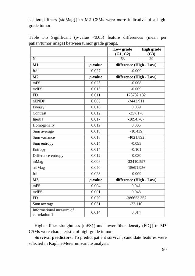
90
scattered fibers (stdMag↓) in M2 CSMs were more indicative of a high-
grade tumor.
Table 5.5 Significant (p-value <0.05) feature differences (mean per
patien/tumor image) between tumor grade groups.
Low grade
(G1, G2)
High grade
(G3)
N 63 29
M1 p-value difference (High - Low)
frd 0.027 -0.009
M2 p-value difference (High - Low)
mFS 0.025 -0.008
mdFS 0.013 -0.009
FD 0.011 178782.182
nENDP 0.005 -3442.911
Energy 0.016 0.039
Contrast 0.012 -357.176
Inertia 0.017 -1094.767
Homogeneity 0.012 0.005
Sum average 0.018 -10.439
Sum variance 0.018 -4021.892
Sum entropy 0.014 -0.095
Entropy 0.014 -0.101
Difference entropy 0.012 -0.030
mMag 0.008 -33410.597
stdMag 0.040 -15691.956
frd 0.028 -0.009
M3 p-value difference (High - Low)
mFS 0.004 0.041
mdFS 0.001 0.043
FD 0.020 -386653.367
Sum average 0.031 -22.110
Informational measure of
correlation 1 0.014 0.014
Higher fiber straightness (mFS↑) and lower fiber density (FD↓) in M3
CSMs were characteristic of high-grade tumors.
Survival predictors. To predict patient survival, candidate features were
selected in Kaplan-Meier univariate analysis.
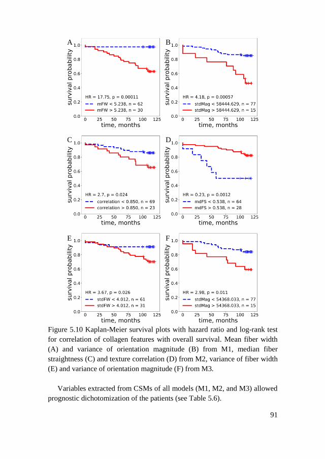
91
Figure 5.10 Kaplan-Meier survival plots with hazard ratio and log-rank test
for correlation of collagen features with overall survival. Mean fiber width
(A) and variance of orientation magnitude (B) from M1, median fiber
straightness (C) and texture correlation (D) from M2, variance of fiber width
(E) and variance of orientation magnitude (F) from M3.
Variables extracted from CSMs of all models (M1, M2, and M3) allowed
prognostic dichotomization of the patients (see Table 5.6).
A B
C D
E F

92
Table 5.6 Univariate analysis
Clinicopathological indicators p-value HR
T category (T1 vs. T2) 0.645 0.81
N category (N0 vs. N1-3) 0.200 1.79
Histological grade (G1 vs. G2-3) 1.000 1.00
Subtype (LumA vs. LumB-LumBHER2+) 0.630 1.24
Age (≤59 vs. >59) 0.062 2.62
M1 p-value HR
mFW <0.001 17.75
mdFW <0.001 9.87
mFS 0.002 5.67
correlation 0.012 5.31
mdFP <0.001 5.12
mdFS 0.001 4.66
mdFL 0.001 4.48
stdMag 0.001 4.18
mFP 0.022 3.79
mFL 0.031 3.14
FD 0.025 2.74
mMag 0.026 2.62
M2 p-value HR
mFS 0.010 3.08
correlation 0.024 2.7
informational measure of correlation 1 0.015 0.35
mdFS 0.001 0.23
M3 p-value HR
sdFW 0.026 3.67
mFW 0.007 3.14
mdFW 0.010 3.06
stdMag 0.011 2.98
sdD 0.019 2.86
mFP 0.031 2.74
mdD 0.025 2.64
mD 0.038 2.56
mdFS 0.031 0.35
CSD 0.004 0.27
CV 0.004 0.27
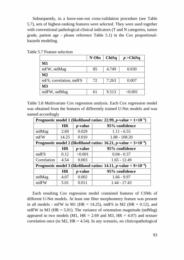
93
Subsequently, in a leave-one-out cross-validation procedure (see Table
5.7), sets of highest-ranking features were selected. They were used together
with conventional pathological-clinical indicators (T and N categories, tumor
grade, patient age - please reference Table 5.1) in the Cox proportional-
hazards modeling.
Table 5.7 Feature selection
N Obs ChiSq p >ChiSq
M1
mFW, stdMag 85 4.749 0.030
M2
mFS, correlation, mdFS 72 7.263 0.007
M3
stdFW, stdMag 61 9.513 <0.001
Table 5.8 Multivariate Cox regression analysis. Each Cox regression model
was obtained from the features of differently trained U-Net models and was
named accordingly
Prognostic model 1 (likelihood ratios: 22.99, p-value = 1×10⁻⁵)
HR p-value 95% confidence
stdMag 2.69 0.029 1.11 - 6.55
mFW 14.25 0.010 1.88 - 108.20
Prognostic model 2 (likelihood ratios: 16.21, p-value = 3×10⁻⁴)
HR p-value 95% confidence
mdFS 0.12 <0.001 0.04 - 0.37
Correlation 4.54 0.003 1.65 - 12.49
Prognostic model 3 (likelihood ratios: 14.11, p-value = 9×10⁻⁴)
HR p-value 95% confidence
stdMag 4.07 0.002 1.66 - 9.97
stdFW 5.01 0.011 1.44 - 17.43
Each resulting Cox regression model contained features of CSMs of
different U-Net models. At least one fiber morphometry feature was present
in all models - mFW in M1 (HR = 14.25), mdFS in M2 (HR = 0.12), and
stdFW in M3 (HR = 5.01). The variance of orientation magnitude (stdMag)
appeared in two models (M1, HR = 2.69 and M3, HR = 4.07) and texture
correlation once (in M2, HR = 4.54). In any scenario, no clinicopathological

94
indicators entered the models (see Table 5.8 for prognostic model details and
Figure 5.10 for Kaplan-Meier plots of prognostic features).
Discussion. In this chapter, the informative value of segmented collagen
framework features was evaluated. It was found that independently trained
U-Net models learned common aspects of tissue collagen architecture,
although all models inherited expert comprehension of collagen
representation via scarce, detailed, or semi-automated annotations. The
trained models generated sets of collagen features that outperformed
conventional clinical indicators in all prognostic models obtained. In general,
it was demonstrated that FCNN-based models can extract essential
information embedded in bright-field pathology images and provide
prognostic value in BC patients.
For ANN to learn representations of collagen organization in a tissue
image, the algorithm needs GT to compute the cross-entropy loss, and guide
the training process. However, collagen, as an annotation object, is of a
complex nature. Dekker et al. [161] assessed breast tumor stromal
organization by manually drawing straight lines along stromal fibers. To
segment collagen deposition in histology images, Jung et al. [162] generated
annotations for ANN semi-automatically by image thresholding and
subsequent manual refinement. To train the M3 ANN model, annotations
similar to Jung et al. [162] were adopted. The approach by Dekker et al.
[161] was expanded to train M1 and M2 ANNs and investigate the influence
of cognitive bias on collagen perception by a human expert. It was
experimentally demonstrated that human visual perception of tissue collagen
framework is highly subjective, as experts’ annotations did differ
significantly by all aspects evaluated (see Table 5.4).
Interestingly, it was noted that ANNs inherited experts’ level of detail.
For example, the means of 10 of 13 Haralick texture features from M2 were
significantly different between tumor grade groups, but only two from M3,
and none from M1 differed significantly. M2, which trained on detailed,
texture-rich annotations, produced collagen framework representations that
reflect tumor growth patterns by the texture features. In contrast, in M1,
which was trained on scarce annotations, the tumor grade is associated with
fractal dimension – a less intuitive and more complex feature that describes
pattern space-filling property. In M3, tumor cell clusters disrupt dense
collagen landscapes and alter the basic geometry of bulk collagen mass;
thus, collagen density and straightness features define tumor shape and are
associated with histological grade.

95
Multiple studies based on second harmonic generation microscopy
quantify local and global tumor collagen arrangement linking it with patient
outcome. High orientation variance, local radial alignment of collagen fibers,
and increased local collagen density were associated with invasion [228] and
poor patient outcomes in breast carcinoma [161, 228-231]. Similarly,
collagen alignment is suggestive of the worse prognosis in pancreatic ductal
adenocarcinoma [232]. In gastric cancer, increased collagen fiber width was
associated with reduced patient survival [233]. Experiments conducted in
this research showed that similar features extracted from bright-field data
allow significant patient stratification into prognostic groups in univariate
analysis. The variance of orientation magnitude (M1: HR = 2.69, p-value =
0.029 & M3: HR = 4.07, p-value = 0.002), mean fiber width (M1: HR =
14.25, p-value = 0.010), the variance of fiber width (M3: HR = 5.01, p-value
= 0.011), median fiber straightness (M2: HR = 0.12, p-value <0.001) and
texture correlation (M2: HR = 4.54, p-value = 0.003), after cross-validation,
serve as independent indicators in multivariate analysis. It is remarkable that
the collagen framework data were extracted from a 1 mm diameter TMA
spot per patient while no conventional clinicopathologic parameters were
needed for the prognostic models (see Table 5.8).
TACS studies [157, 228] revealed exceptional prognostic information
embedded in the collagen framework. The results presented here are in line
with the concept of TACS. Latent correlations characterizing collagen
arrangement in our CSMs were highly concordant between ANN models.
Four factors were noted where the same features from all trained models
combined (Factors 3, 6, 7, 8 see Figure 5.9). TACS-1 (increased collagen
deposition) resembles Factor 3, where means and standard deviations of
distances between collagen endpoints (a measure of density) accumulated.
Similarly, TACS-2 (straightened fibers aligned to the tumor boundary) can
be observed in Factor 6 (and less clearly in Factor 8), formed by lacunarity, a
measure of gappiness. Finally, TACS-3 (radially aligned collagen fibers) can
be assumed in Factor 7, represented by standard deviations of orientation
angles.
5.3. Chapter Conclusions
A novel FCNN-based approach for TME collagen segmentation was
developed. Differently trained models produced highly concordant collagen
segmentation masks. IoU of collagen segmentations averaged over the whole
dataset varied from 0.4 up to over 0.6. The averaged ratio of segmentation
96
areas by different models ranged from 0.5 up to 1.2, and the average
common area covered by all segmentations ranged from 0.6 up to 1.0.
Principles governing collagen framework arrangement in tumorous tissue
were assessed by factor analysis and confirmed to be in line with the
established tumor-associated collagen signature paradigm. Eight independent
factors (with eigenvalues ≥1) explain 86.2% of the variance in the data.
Density, fractal, and orientation features from all assessed models aggregate
in orthogonally independent factors (with correlation coefficients over 0.7).
Features extracted from the collagen architecture detected by all trained
models differed significantly (p-value <0.05) between tumor grade groups.
This fact suggests that all segmentation models independently capture
aggressive tumor growth patterns by different features.
Given the ambiguity of collagen ground truth in bright-field microscopy
images, the biological meaningfulness of collagen segmentations had to be
proven by patient prognostication. Morphometric features extracted from
collagen segmentations by all trained CNNs achieved reliable prognostic
models (with likelihood ratios 14.11-22.99, p-value <0.05), and no
established clinicopathological indicators were needed for breast cancer
patients’ prognostication.
97
6. MULTIPLE CLASS HISTOPATHOLOGY OBJECT
SEGMENTATION FOR TUMOR CLASSIFICATION
Previous chapters touched upon different tumor histology object
detection, segmentation, and classification. While Chapter 3 explored the
classification of tumorous tissue regions into two major compartments -
tumor epithelium and stroma, Chapter 4 introduced immune infiltrate
(lymphocyte) detection and precise segmentation, and Chapter 5 added a
method to segment and describe fibrous collagen in TME. This chapter is
dedicated to exploring the segmentation of multiple histology objects from
routine bright-field histology images of breast tumor tissue by an FCNN-
based model. The motivation for detailed tumor deconstruction into
histology primitives rises from the determination to formulate patient-level
medical decision-making by objective, accurate, and standardized
phenotyping of the disease’s microscopic manifestations.
6.1. Experiment Design
This chapter presents a technique enabling simultaneous segmentation
and identification of lymphocytes and dense immune infiltrates, tumor cell
nuclei and tumorous tissue area, stromal cell nuclei and stromal tissue
compartment, and TME collagen carcass from H&E-stained tumor tissue
WSIs.
First, an image sampling strategy is proposed by introducing a tissue
detector. A training dataset representing various tissue compartments is
created by tissue zoning to train the segmentation model effectively. The
training dataset of 256×256 pixel-sized image patches is thoroughly
annotated by an expert highlighting four object classes - lymphocyte nuclei,
tumor cell nuclei, stromal cell nuclei, and collagen fibers. Annotation masks
are stacked to create multichannel ground truth masks. Additional four
annotation channels are generated in an automated way - for nuclei of each
type (and for all nuclei together), filling gaps between nuclei within the
predetermined proximity to each other.
Then, an FCNN-based approach utilizing multichannel GT and multi-
layer outputs is considered for the simultaneous segmentation of multiple
histologic objects. The base model employed is a modified U-Net (described
in detail in Chapter 5.1.3). An ensemble of weighted loss functions is
explored to train the model.

98
Segmented histologic objects are subjected to morphometric analysis to
build robust tissue-describing feature space. A set of 20 histology image
features (nuclei densities, collagen fiber geometry, orientation, density, and
texture) is extracted from segmentation masks.
To analyze the complete tumor tissue captured in a WSI tissue detector is
applied, tissue containing region coordinates are acquired, and WSI is
analyzed patch by patch. Segmented object morphometric features are
aggregated into feature maps. To produce pathology endpoints, ML
algorithms always require structured data. Although morphometric maps are
very informative and can be appreciated visually, WSIs of different image
plane sizes and varying tissue shapes and placement on a slide cannot be
considered structured data. Morphometric map as a representation of WSI is
not suitable for straightforward classification by ML models. A unified
spatial relationship between tissue compartments preserving WSI
representation is proposed to tackle the WSI classification problem.
The proposed method was tested in an international challenge. The
challenge raised the task to predict specific breast tumor biomarker (HER2)
status (pathology endpoint applicable to the whole tumor sample to select
patients reliable for targeted therapy) for a set of routine H&E-stained breast
tumor tissue WSIs. In a diagnostic pathology workup, this endpoint is only
available by additional and special tissue processing, which means that
human experts cannot reliably infer HER2 biomarker status from tissue
morphology captured in routine H&E slides.
For each WSI in training and testing sets, WSI projections are generated.
To predict the HER2 status deep neural network model (Xception [234]
architecture) is trained, and WSIs in a testing set are classified as being
HER2-positive or HER2-negative.
6.1.1. Dataset
Images. In this experiment, a set of 510 routine tissue slides (H&E-
stained breast cancer tumor tissue WSIs) were used. Slides were obtained
from the HEROHE Challenge [235]. Images of H&E-stained tissue slides
were scanned at 20× optical magnification and saved in the MIRAX file
format. The HEROHE Challenge was organized to promote computational
techniques to assess biomarker status in tumor images acquired from routine
tissue slides. Organizers provided two WSI datasets – a training set
composed of 360 cases (144 biomarker-positive) and a test set composed of

99
150 cases. Experienced pathologists assessed biomarker status for each case
according to the latest guidelines for breast cancer.
Image sampling. An overall scheme for data preparation is given in
Figure 6.1. Firstly, a tissue segmentation map is created with three tissue
zones: deep tumor, deep stroma, and an intermediate zone (roughly
corresponding to IM). To achieve this tissue zoning an average pooling is
applied to an original image (Figure 6.1, box 1) by sliding a 256×256
window. The resulting thumbnail image (Figure 6.1, box 2) is subjected to
create a thumbnail representation in an artificial stain color space (Figure
6.1, box 3) by converting the color space from RGB to HED stain colors
(Haematoxylin, Eosin, DAB) using the skimage library in Python [225].
Thumbnail HED representation is thresholded and normalized to the unit
interval [0, 1], the DAB channel is discarded. Finally, tissue detection and
zoning are achieved by k-means clustering (number of clusters = 4) on H and
E channels of HED representation. Each pixel in a tissue segmentation map
(Figure 6.1, box 4) corresponds to a 256×256 pixel-sized patch in an original
WSI (Figure 6.1, box 5).
Figure 6.1 Data preparation scheme.
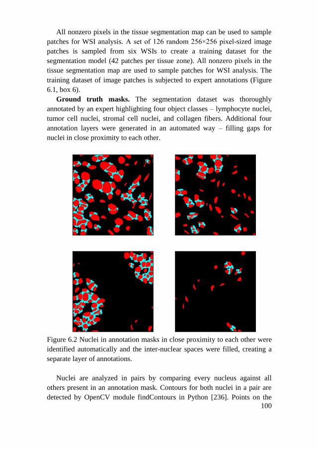
100
All nonzero pixels in the tissue segmentation map can be used to sample
patches for WSI analysis. A set of 126 random 256×256 pixel-sized image
patches is sampled from six WSIs to create a training dataset for the
segmentation model (42 patches per tissue zone). All nonzero pixels in the
tissue segmentation map are used to sample patches for WSI analysis. The
training dataset of image patches is subjected to expert annotations (Figure
6.1, box 6).
Ground truth masks. The segmentation dataset was thoroughly
annotated by an expert highlighting four object classes – lymphocyte nuclei,
tumor cell nuclei, stromal cell nuclei, and collagen fibers. Additional four
annotation layers were generated in an automated way – filling gaps for
nuclei in close proximity to each other.
Figure 6.2 Nuclei in annotation masks in close proximity to each other were
identified automatically and the inter-nuclear spaces were filled, creating a
separate layer of annotations.
Nuclei are analyzed in pairs by comparing every nucleus against all
others present in an annotation mask. Contours for both nuclei in a pair are
detected by OpenCV module findContours in Python [236]. Points on the

101
contours of both nuclei within the predefined distance are saved to the
proximity mask. Morphological dilation (with 8×8 pixel elliptical kernel) is
applied to fill in the gap between saved contour points. Finally, the nuclei
annotation mask is subtracted from the proximity mask to ensure that the
nuclei mask does not overlap the proximity mask. Both nuclei and the
resulting proximity masks are saved to the multi-channel annotation array as
separate layers (see Figure 6.2). The proximity cutoff was set to 8 pixels
(selected by a careful calibration). The gap-filling procedure is applied to
masks of nuclei of each type (lymphocytes, tumor cells, stromal cells)
separately, resulting in three additional layers of GT. One more layer of GT
is produced by applying gap filling to the total nuclei mask.
6.1.2. U-Net Segmentation Model
A modified U-Net-based model (described in Chapter 5.1.3) was trained
to segment targeted histologic objects. The network was modified to output
an 8-layered segmentation map (one segmentation layer for each manual
annotation class and one for each class generated by gap-filling). The model
was set to minimize an ensemble loss function (see formula 6.2) – a
combination of different weighted loss functions (intersection over union
loss (see formula in 6.1), binary cross-entropy loss, mean square error loss,
total variance loss [210, 237]) with adaptive moment estimation using
default parameters provided in the original method [204].:
𝐼𝑜𝑈𝐿 = 1 −𝑇𝑃
𝐹𝑃+𝑇𝑃+𝐹𝑁 (6.1) ,
𝑙𝑜𝑠𝑠 = 𝑤1 ∗ 𝐵𝐶𝐿 + 𝑤2 ∗ 𝑀𝑆𝐸 + 𝑤3 ∗ 𝑇𝑉𝐿 + 𝑤4 ∗ 𝐼𝑜𝑈𝐿 (6.2)
where BCL is binary cross-entropy loss, MSE is mean square error, TVL is
total variance loss, IoUL is intersection over union loss.
The model trained on single patch batches, and the dataset of annotated
patches was split into training subset (50%) and validation subset (50%) to
complicate the learning by moving the stress to the validation step. The
algorithm was set to save model weights after each improvement in
validation loss, and terminate the training phase after validation loss did not
improve for 100 consecutive epochs or after 200 epochs passed.
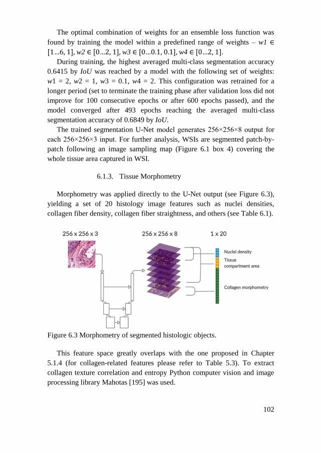
102
The optimal combination of weights for an ensemble loss function was
found by training the model within a predefined range of weights – w1 ∈
[1…6,1],w2 ∈[0…2,1],w3 ∈[0…0.1,0.1], w4 ∈[0…2,1].
During training, the highest averaged multi-class segmentation accuracy
0.6415 by IoU was reached by a model with the following set of weights:
w1 = 2, w2 = 1, w3 = 0.1, w4 = 2. This configuration was retrained for a
longer period (set to terminate the training phase after validation loss did not
improve for 100 consecutive epochs or after 600 epochs passed), and the
model converged after 493 epochs reaching the averaged multi-class
segmentation accuracy of 0.6849 by IoU.
The trained segmentation U-Net model generates 256×256×8 output for
each 256×256×3 input. For further analysis, WSIs are segmented patch-by-
patch following an image sampling map (Figure 6.1 box 4) covering the
whole tissue area captured in WSI.
6.1.3. Tissue Morphometry
Morphometry was applied directly to the U-Net output (see Figure 6.3),
yielding a set of 20 histology image features such as nuclei densities,
collagen fiber density, collagen fiber straightness, and others (see Table 6.1).
Figure 6.3 Morphometry of segmented histologic objects.
This feature space greatly overlaps with the one proposed in Chapter
5.1.4 (for collagen-related features please refer to Table 5.3). To extract
collagen texture correlation and entropy Python computer vision and image
processing library Mahotas [195] was used.
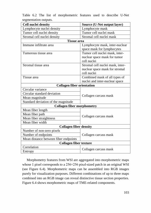
103
Table 6.2 The list of morphometric features used to describe U-Net
segmentation outputs.
Cell nuclei density Source (U-Net output layer)
Lymphocyte nuclei density Lymphocyte mask
Tumor cell nuclei density Tumor cell nuclei mask
Stromal cell nuclei density Stromal cell nuclei mask
Tissue area
Immune infiltrate area Lymphocyte mask, inter-nuclear
space mask for lymphocytes
Tumorous tissue area Tumor cell nuclei mask, inter-
nuclear space mask for tumor
cell nuclei
Stromal tissue area Stromal cell nuclei mask, inter-
nuclear space mask for stromal
cell nuclei
Tissue area Combined mask of all types of
nuclei and inter-nuclear space
Collagen fiber orientation
Circular variance
Collagen carcass mask Circular standard deviation
Mean magnitude
Standard deviation of the magnitude
Collagen fiber morphometry
Mean fiber length
Collagen carcass mask Mean fiber path
Mean fiber straightness
Mean fiber width
Collagen fiber density
Number of non-zero pixels
Collagen carcass mask Number of endpoints
Mean distance between fiber endpoints
Collagen fiber texture
Correlation Collagen carcass mask
Entropy
Morphometry features from WSI are aggregated into morphometric maps
whose 1 pixel corresponds to a 256×256 pixel-sized patch in an original WSI
(see Figure 6.4). Morphometric maps can be assembled into RGB images
purely for visualization purposes. Different combinations of up to three maps
combined into an RGB image can reveal distinctive tissue section properties.
Figure 6.4 shows morphometric maps of TME-related components.
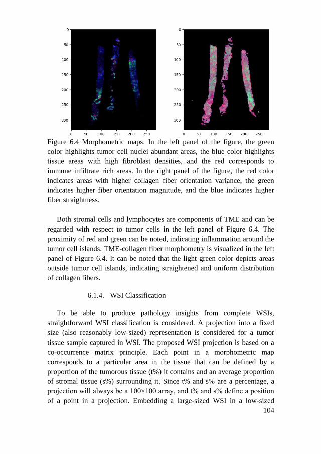
104
Figure 6.4 Morphometric maps. In the left panel of the figure, the green
color highlights tumor cell nuclei abundant areas, the blue color highlights
tissue areas with high fibroblast densities, and the red corresponds to
immune infiltrate rich areas. In the right panel of the figure, the red color
indicates areas with higher collagen fiber orientation variance, the green
indicates higher fiber orientation magnitude, and the blue indicates higher
fiber straightness.
Both stromal cells and lymphocytes are components of TME and can be
regarded with respect to tumor cells in the left panel of Figure 6.4. The
proximity of red and green can be noted, indicating inflammation around the
tumor cell islands. TME-collagen fiber morphometry is visualized in the left
panel of Figure 6.4. It can be noted that the light green color depicts areas
outside tumor cell islands, indicating straightened and uniform distribution
of collagen fibers.
6.1.4. WSI Classification
To be able to produce pathology insights from complete WSIs,
straightforward WSI classification is considered. A projection into a fixed
size (also reasonably low-sized) representation is considered for a tumor
tissue sample captured in WSI. The proposed WSI projection is based on a
co-occurrence matrix principle. Each point in a morphometric map
corresponds to a particular area in the tissue that can be defined by a
proportion of the tumorous tissue (t%) it contains and an average proportion
of stromal tissue (s%) surrounding it. Since t% and s% are a percentage, a
projection will always be a 100×100 array, and t% and s% define a position
of a point in a projection. Embedding a large-sized WSI in a low-sized
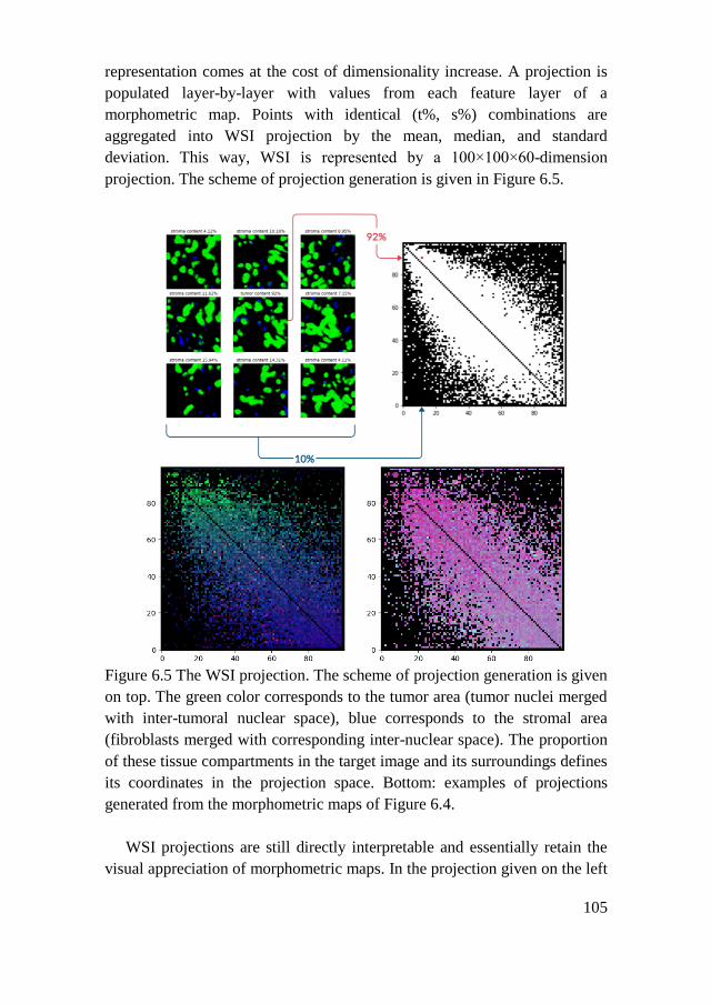
105
representation comes at the cost of dimensionality increase. A projection is
populated layer-by-layer with values from each feature layer of a
morphometric map. Points with identical (t%, s%) combinations are
aggregated into WSI projection by the mean, median, and standard
deviation. This way, WSI is represented by a 100×100×60-dimension
projection. The scheme of projection generation is given in Figure 6.5.
Figure 6.5 The WSI projection. The scheme of projection generation is given
on top. The green color corresponds to the tumor area (tumor nuclei merged
with inter-tumoral nuclear space), blue corresponds to the stromal area
(fibroblasts merged with corresponding inter-nuclear space). The proportion
of these tissue compartments in the target image and its surroundings defines
its coordinates in the projection space. Bottom: examples of projections
generated from the morphometric maps of Figure 6.4.
WSI projections are still directly interpretable and essentially retain the
visual appreciation of morphometric maps. In the projection given on the left

106
panel of Figure 6.5, red dots corresponding to lymphocyte density stay close
to the green cluster of dense tumor cells (↑t%, ↓s%) but do not penetrate
deep inside it and are mainly dispersed among blue dots corresponding to
stromal cells (↓t%, ↑s%). Notably, this representation forces differently sized
WSIs to be structured identically with fixed dimensions. Therefore, WSI
projections enable straightforward WSI classification by virtually any ML
classifier model.
The Xception [234] model was trained to predict tumor HER2 biomarker
status. The training dataset was randomly split into training subset (80%)
and validation subset (20%) and the model was trained on single sample
batches. The objective of the challenge was to produce both soft and hard
predictions about the biomarker status of a specimen. Therefore binary
cross-entropy loss was used to guide the training. The algorithm was set to
save model weights after each improvement in validation loss and terminate
the training phase after validation loss did not improve for 20 consecutive
epochs.
For DL TensorFlow framework in Python was used [198]. Full training
of the model was performed on a high-performance graphical processing
unit (Nvidia GeForce GTX1080).
Feature extraction and quantification were implemented using the
computer vision and image processing libraries scikit-image [225], Mahotas
[195] and OpenCV [236] in Python.
6.2. Results
To predict the HER2 status of the tumor at the WSI level, WSIs were
processed by the method presented in this chapter. For each WSI in training
and testing sets, morphometric feature maps were generated as described in
Chapter 6.1.3. To predict the HER2 status WSI projections were generated
as described in Chapter 6.1.4. The deep neural network model (Xception
[234] architecture) was trained, and WSIs in a testing set were classified as
being HER2-positive or HER2-negative.
6.2.1. WSI Segmentation
The image sampling strategy presented in Chapter 6.1.1 (Fig. 6.1) was
applied to select a set of 126 random 256×256 pixel-sized image patches
from 6 WSIs from the testing set to create a training dataset for the
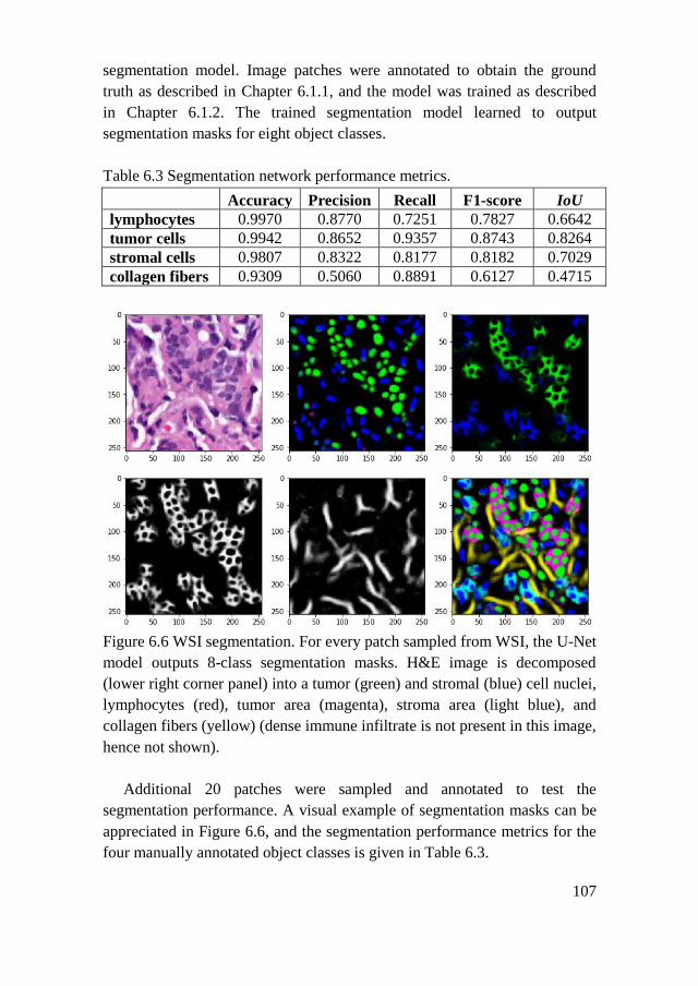
107
segmentation model. Image patches were annotated to obtain the ground
truth as described in Chapter 6.1.1, and the model was trained as described
in Chapter 6.1.2. The trained segmentation model learned to output
segmentation masks for eight object classes.
Table 6.3 Segmentation network performance metrics.
Accuracy Precision Recall F1-score IoU
lymphocytes 0.9970 0.8770 0.7251 0.7827 0.6642
tumor cells 0.9942 0.8652 0.9357 0.8743 0.8264
stromal cells 0.9807 0.8322 0.8177 0.8182 0.7029
collagen fibers 0.9309 0.5060 0.8891 0.6127 0.4715
Figure 6.6 WSI segmentation. For every patch sampled from WSI, the U-Net
model outputs 8-class segmentation masks. H&E image is decomposed
(lower right corner panel) into a tumor (green) and stromal (blue) cell nuclei,
lymphocytes (red), tumor area (magenta), stroma area (light blue), and
collagen fibers (yellow) (dense immune infiltrate is not present in this image,
hence not shown).
Additional 20 patches were sampled and annotated to test the
segmentation performance. A visual example of segmentation masks can be
appreciated in Figure 6.6, and the segmentation performance metrics for the
four manually annotated object classes is given in Table 6.3.

108
6.2.2. WSI Classification
For each WSI in training and testing sets, morphometric feature maps
were generated and used to transform WSIs into WSI projections. The
Xception model was trained to predict tumor HER2 biomarker status using a
training set composed of 360 cases (144 HER2-positive). The training
dataset was randomly split into training subset (280 WSIs, 80%) and
validation subset (80 WSIs, 20%), and the model was tested by training with
three optimizers (see Figure 6.7) - stochastic gradient descent (SGD [238]),
Adam [204], and Adadelta [239] with default parameter values provided in
the original method (available in Keras API [199]).
Figure 6.7 Classifier training metrics. Dashed line depicts training phase,
continuous line depicts validation phase (bold lines for validation data are
shown as exponentially smoothed moving average to highlight the trend).
Red dots indicate the point of convergence (last improvement of validation
loss). Blue lines - SGD, green lines - Adam, orange - Adadelta.
The Xception model trained with SGD optimizer achieved higher
validation accuracy (0.5327, after 16 epochs) than with Adam (0.3645, after
16 epochs) or Adadelta (0.3556, after 26 epochs) optimizers (see Figure 6.7).
6.2.3. Evaluation
A test set composed of 150 unknown HER2 status cases was analyzed as
presented in this chapter and the results were submitted for evaluation.
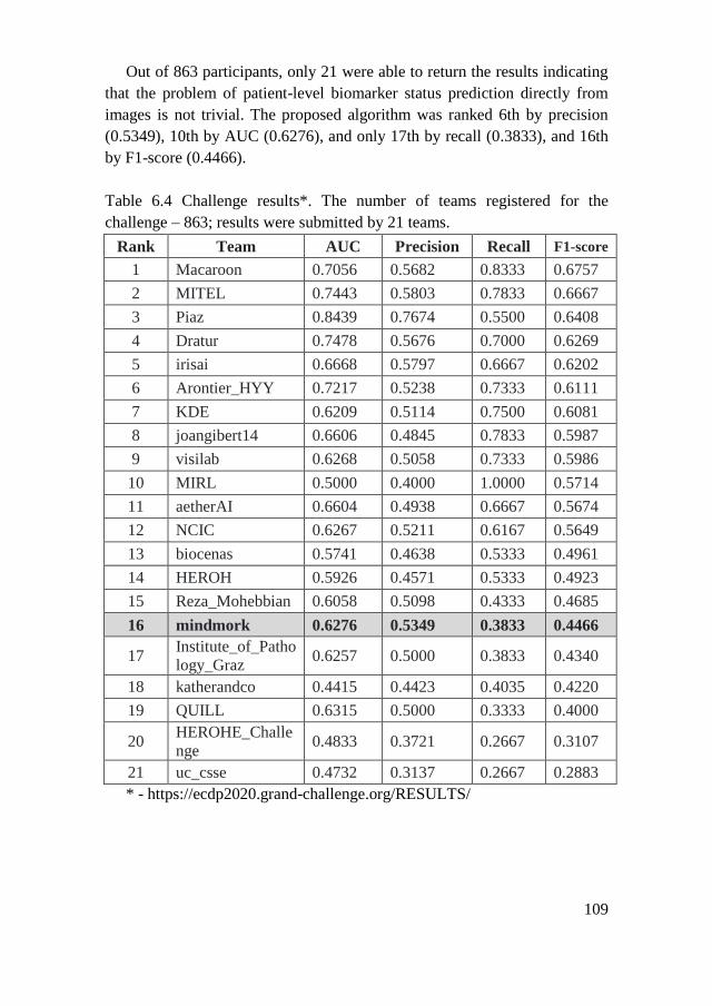
109
Out of 863 participants, only 21 were able to return the results indicating
that the problem of patient-level biomarker status prediction directly from
images is not trivial. The proposed algorithm was ranked 6th by precision
(0.5349), 10th by AUC (0.6276), and only 17th by recall (0.3833), and 16th
by F1-score (0.4466).
Table 6.4 Challenge results*. The number of teams registered for the
challenge – 863; results were submitted by 21 teams.
Rank Team AUC Precision Recall F1-score
1 Macaroon 0.7056 0.5682 0.8333 0.6757
2 MITEL 0.7443 0.5803 0.7833 0.6667
3 Piaz 0.8439 0.7674 0.5500 0.6408
4 Dratur 0.7478 0.5676 0.7000 0.6269
5 irisai 0.6668 0.5797 0.6667 0.6202
6 Arontier_HYY 0.7217 0.5238 0.7333 0.6111
7 KDE 0.6209 0.5114 0.7500 0.6081
8 joangibert14 0.6606 0.4845 0.7833 0.5987
9 visilab 0.6268 0.5058 0.7333 0.5986
10 MIRL 0.5000 0.4000 1.0000 0.5714
11 aetherAI 0.6604 0.4938 0.6667 0.5674
12 NCIC 0.6267 0.5211 0.6167 0.5649
13 biocenas 0.5741 0.4638 0.5333 0.4961
14 HEROH 0.5926 0.4571 0.5333 0.4923
15 Reza_Mohebbian 0.6058 0.5098 0.4333 0.4685
16 mindmork 0.6276 0.5349 0.3833 0.4466
17 Institute_of_Patho
logy_Graz 0.6257 0.5000 0.3833 0.4340
18 katherandco 0.4415 0.4423 0.4035 0.4220
19 QUILL 0.6315 0.5000 0.3333 0.4000
20 HEROHE_Challe
nge 0.4833 0.3721 0.2667 0.3107
21 uc_csse 0.4732 0.3137 0.2667 0.2883
* - https://ecdp2020.grand-challenge.org/RESULTS/
110
6.3. Chapter Conclusions
This chapter described the integration of tumor-centric and TME-centric
segmentation algorithms utilizing experience and knowledge gained in
previous experiments.
An aggregated segmentation method was presented. Segmentation of
multiple histologic objects in a single FCNN-based model was achieved by
leveraging multichannel ground truth and multilayer outputs of the model.
During training, the model reached an averaged multi-class segmentation
accuracy of 0.6849 as assessed by IoU.
The transformation of a WSI was proposed to enable deep neural network
training regardless of WSI size while keeping spatial relationships between
tissue compartments. The proposed transformation allows achieving
competitive biomarker status prediction results of AUC score 0.6276 and F1-
score 0.4466.
111
GENERAL CONCLUSIONS
Literature analysis revealed that tumor microenvironment related object
segmentation and classification is somewhat neglected in digital pathology,
especially when analysing commonly in routine pathology diagnostics H&E-
stained tissue WSI scans.
A superpixel-based annotation approach of H&E-stained tissue WSI data
for tumor epithelium-stroma classification was introduced. Conventional
classifiers such as support vector machine, random decision forest, and
multilayer perceptron showed quite similar performance ranging from AUC
0.9533 to 0.9666. The best result was obtained by a multilayer perceptron.
Color space has an impact on superpixel classification accuracy. Adding
superpixel color features allows an increase of classification accuracy in
terms of AUC from 0.9542 up to 0.9666 when compared to texture features
only. However, the best AUC of 0.9895 was obtained by the CNN classifier
trained on patched image data and showed the best generalization properties
among investigated classifiers.
A lightweight method having good generalization properties for cell
nuclei segmentation and consecutive lymphocyte classification in H&E-
stained breast and colorectal cancer WSIs was proposed.
● The modified shallow U-Net architecture supplemented with
multiple-input layers and the introduced convolutional texture
blocks allowed to obtain a lower model complexity than original U-
Net and Micro-Net models and achieved higher nuclei segmentation
Dice accuracy reaching 0.80 compared to those 0.78 and 0.79
obtained by the U-Net and Micro-Net models respectively while
training on nuclei masks only. Further the architecture performance
was increased to 0.81 when trained on nuclei masks supplemented
with an active contour layer.
● Multilayer perceptron produced the best results among the tested
lymphocytes classifiers with a classification accuracy of 0.78 –
higher than those obtained by the random forest classifier and CNN
producing accuracy of 0.77 and 0.76 respectively.
● The proposed method for nuclei segmentation and classification by
modified U-Net architecture was tested on a public dataset and
showed good generalization properties. The obtained 0.71
lymphocyte classification accuracy was even more increased up to

112
0.81 by introducing stain normalization procedure. The obtained
results are comparable to the state-of-the-art lymphocyte detection
methods but provide an additional lymphocyte segmentation
capability.
A deep neural network architecture was introduced for tumor
microenvironment collagen segmentation.
● Independent instances of models were trained on highly differing
annotations and reached consensus by producing highly concordant
collagen segmentation masks as assessed by IoU (0.4 – 0.6), the
ratio of segmentation areas (0.5 – 1.2), and the common area
covered by all segmentations (0.6 – 1.0). The analysis revealed that
tumor grade, a feature of a tumor that in routine practice is only
inferred visually by a human expert, can be determined by collagen
features. Trained models independently captured aggressive tumor
growth patterns by significantly emphasizing different collagen
features as determined by the analysis of collagen feature variance
between tumor grade groups with ANOVA test having p-value
<0.05. Accomplished factor analysis confirmed collagen
arrangement governing principles after the segmentation step.
● Collagen features such as fiber orientation and morphometry
currently available only by specialized tissue imaging techniques
were extracted from collagen segmentation maps produced by the
proposed method and were confirmed to be reliable by prognostic
modeling with obtained likelihood ratio interval 14.11-22.99, at p-
value <0.05. The results suggest that the above-mentioned features
after careful analysis have the potential to be implemented in routine
pathology diagnostics.
A modified U-Net architecture proposed for collagen segmentation was
further generalized to segment eight tumorous tissue components from
routine H&E-stained breast tissue WSIs at the same step by utilizing multi-
channel ground truth masks. The trained model achieved a reasonably
accurate multi-class segmentation IoU of 0.6849. A whole-slide image
transformation that retains spatial relationships between the segmented
tumor tissue components was introduced by constructing an image feature
space based on explicit morphometry rules applied to the eight segmented
object classes of the tumorous tissue. The introduced transformation embeds
a whole-slide image into a projection of fixed dimensions that allows any
113
machine learning classifier that works on predefined input data sizes to be
trained on complete whole-slide images of arbitrary sizes. The complete
workflow consisting of a generalized multi-class segmentation model,
proposed WSI transformation, and a trained WSI projection classifier
achieved competitive tumor biomarker prediction results having AUC and
F1 scores 0.6276 and 0.4466 respectively.

114
REFERENCES
[1] A. T. Feldman and D. Wolfe, "Tissue Processing and Hematoxylin
and Eosin Staining," in Histopathology: Methods and Protocols, C.
E. Day Ed. New York, NY: Springer New York, pp. 31-43, 2014.
[2] E. R. Malone, M. Oliva, P. J. B. Sabatini, T. L. Stockley, and L. L.
Siu, "Molecular profiling for precision cancer therapies," Genome
Medicine, vol. 12, no. 1, p. 8, 2020, doi: 10.1186/s13073-019-0703-
1.
[3] S. Brassart-Pasco, S. Brezillon, B. Brassart, L. Ramont, J. B. Oudart,
and J. C. Monboisse, "Tumor Microenvironment: Extracellular
Matrix Alterations Influence Tumor Progression," Frontiers in
Oncology, Mini Review vol. 10, no. 397, p. 397, 2020, doi:
10.3389/fonc.2020.00397.
[4] R. Baghban et al., "Tumor microenvironment complexity and
therapeutic implications at a glance," Cell Communication and
Signaling, vol. 18, no. 1, p. 59, 2020, doi: 10.1186/s12964-020-
0530-4.
[5] A. Labani-Motlagh, M. Ashja-Mahdavi, and A. Loskog, "The
Tumor Microenvironment: A Milieu Hindering and Obstructing
Antitumor Immune Responses," Frontiers in Immunology, Review
vol. 11, no. 940, p. 940, 2020, doi: 10.3389/fimmu.2020.00940.
[6] B. Allard et al., "Immuno-oncology-101: overview of major
concepts and translational perspectives," Seminars in Cancer
Biology, vol. 52, no. Pt 2, pp. 1-11, 2018, doi:
10.1016/j.semcancer.2018.02.005.
[7] K. C. Valkenburg, A. E. de Groot, and K. J. Pienta, "Targeting the
tumour stroma to improve cancer therapy," Nature Reviews: Clinical
Oncology, vol. 15, no. 6, pp. 366-381, 2018, doi: 10.1038/s41571-
018-0007-1.
[8] R. R. Somani and U. V. Bhanushali, "Targeting angiogenesis for
treatment of human cancer," Indian Journal of Pharmaceutical
Sciences, vol. 75, no. 1, pp. 3-10, 2013, doi: 10.4103/0250-
474X.113529.
[9] S. Y. Gun, S. W. L. Lee, J. L. Sieow, and S. C. Wong, "Targeting
immune cells for cancer therapy," Redox Biology, vol. 25, p.
101174, 2019, doi: 10.1016/j.redox.2019.101174.
[10] J. Galon et al., "Cancer classification using the Immunoscore: a
worldwide task force," Journal of Translational Medicine, vol. 10,
no. 1, p. 205, 2012, doi: 10.1186/1479-5876-10-205.
[11] J. Saltz et al., "Spatial Organization and Molecular Correlation of
Tumor-Infiltrating Lymphocytes Using Deep Learning on Pathology
Images," Cell Reports, vol. 23, no. 1, pp. 181-193 e187, 2018, doi:
10.1016/j.celrep.2018.03.086.
115
[12] A. N. Basavanhally et al., "Computerized image-based detection and
grading of lymphocytic infiltration in HER2+ breast cancer
histopathology," IEEE Transactions on Biomedical Engineering,
vol. 57, no. 3, pp. 642-653, 2010, doi:
10.1109/TBME.2009.2035305.
[13] J. Chen and C. Srinivas, "Automatic Lymphocyte Detection in H&E
Images with Deep Neural Networks," ArXiv, vol. abs/1612.03217,
2016.
[14] A. Mouelhi, H. Rmili, J. B. Ali, M. Sayadi, R. Doghri, and K. Mrad,
"Fast unsupervised nuclear segmentation and classification scheme
for automatic allred cancer scoring in immunohistochemical breast
tissue images," Computer Methods and Programs in Biomedicine,
vol. 165, pp. 37-51, 2018, doi: 10.1016/j.cmpb.2018.08.005.
[15] M. Veta, P. J. van Diest, R. Kornegoor, A. Huisman, M. A.
Viergever, and J. P. Pluim, "Automatic nuclei segmentation in H&E
stained breast cancer histopathology images," PloS One, vol. 8, no.
7, p. e70221, 2013, doi: 10.1371/journal.pone.0070221.
[16] T. M. Bauman et al., "Characterization of fibrillar collagens and
extracellular matrix of glandular benign prostatic hyperplasia
nodules," PloS One, vol. 9, no. 10, p. e109102, 2014, doi:
10.1371/journal.pone.0109102.
[17] M. Wolman and F. H. Kasten, "Polarized light microscopy in the
study of the molecular structure of collagen and reticulin,"
Histochemistry, vol. 85, no. 1, pp. 41-49, 1986, doi:
10.1007/BF00508652.
[18] K. A. Wegner, A. Keikhosravi, K. W. Eliceiri, and C. M. Vezina,
"Fluorescence of Picrosirius Red Multiplexed With
Immunohistochemistry for the Quantitative Assessment of Collagen
in Tissue Sections," Journal of Histochemistry and Cytochemistry,
vol. 65, no. 8, pp. 479-490, 2017, doi: 10.1369/0022155417718541.
[19] C. Saillard et al., "Predicting Survival After Hepatocellular
Carcinoma Resection Using Deep Learning on Histological Slides,"
Hepatology, vol. 72, no. 6, pp. 2000-2013, 2020, doi:
10.1002/hep.31207.
[20] R. Yamashita, J. Long, A. Saleem, D. L. Rubin, and J. Shen, "Deep
learning predicts postsurgical recurrence of hepatocellular
carcinoma from digital histopathologic images," Scientific Reports,
vol. 11, no. 1, p. 2047, 2021, doi: 10.1038/s41598-021-81506-y.
[21] R. R. Rawat et al., "Deep learned tissue "fingerprints" classify breast
cancers by ER/PR/Her2 status from H&E images," Scientific
Reports, vol. 10, no. 1, p. 7275, 2020, doi: 10.1038/s41598-020-
64156-4.

116
[22] P. C. Nowell, "The clonal evolution of tumor cell populations,"
Science, vol. 194, no. 4260, pp. 23-28, 1976, doi:
10.1126/science.959840.
[23] A. Fortunato, A. Boddy, D. Mallo, A. Aktipis, C. C. Maley, and J.
W. Pepper, "Natural Selection in Cancer Biology: From Molecular
Snowflakes to Trait Hallmarks," Cold Spring Harbor Perspectives
in Medicine, vol. 7, no. 2, p. a029652, 2017, doi:
10.1101/cshperspect.a029652.
[24] L. Koch, "Cancer genomics: The driving force of cancer evolution,"
Nat Rev Genet, vol. 18, no. 12, p. 703, 2017, doi:
10.1038/nrg.2017.95.
[25] T. Goto, Y. Hirotsu, K. Amemiya, H. Mochizuki, and M. Omata,
"Understanding Intratumor Heterogeneity and Evolution in NSCLC
and Potential New Therapeutic Approach," Cancers, vol. 10, no. 7,
p. 212, 2018, doi: 10.3390/cancers10070212.
[26] M. Greaves and C. C. Maley, "Clonal evolution in cancer," Nature,
vol. 481, no. 7381, pp. 306-313, 2012, doi: 10.1038/nature10762.
[27] M. Casas-Selves and J. Degregori, "How cancer shapes evolution,
and how evolution shapes cancer," Evolution (N Y), vol. 4, no. 4, pp.
624-634, 2011, doi: 10.1007/s12052-011-0373-y.
[28] D. Hanahan and R. A. Weinberg, "The hallmarks of cancer," Cell,
vol. 100, no. 1, pp. 57-70, 2000, doi: 10.1016/s0092-
8674(00)81683-9.
[29] E. Solary and L. Laplane, "The role of host environment in cancer
evolution," Evolutionary Applications, vol. 13, no. 7, pp. 1756-1770,
2020, doi: 10.1111/eva.13039.
[30] D. Hanahan and R. A. Weinberg, "Hallmarks of cancer: the next
generation," Cell, vol. 144, no. 5, pp. 646-674, 2011, doi:
10.1016/j.cell.2011.02.013.
[31] H. Peinado et al., "Pre-metastatic niches: organ-specific homes for
metastases," Nature Reviews: Cancer, vol. 17, no. 5, pp. 302-317,
2017, doi: 10.1038/nrc.2017.6.
[32] S. Paget, "The Distribution of Secondary Growths in Cancer of the
Breast," The Lancet, vol. 133, no. 3421, pp. 571-573, 1889, doi:
10.1016/s0140-6736(00)49915-0.
[33] R. Virchow, "Cellular pathology. As based upon physiological and
pathological histology. Lecture XVI--Atheromatous affection of
arteries. 1858," Nutrition Reviews, vol. 47, no. 1, pp. 23-25, 1989,
doi: 10.1111/j.1753-4887.1989.tb02747.x.
[34] M. A. Morse, S. Chui, A. Hobeika, H. K. Lyerly, and T. Clay,
"Recent developments in therapeutic cancer vaccines," Nature
Clinical Practice: Oncology, vol. 2, no. 2, pp. 108-113, 2005, doi:
10.1038/ncponc0098.

117
[35] K. M. Hargadon, C. E. Johnson, and C. J. Williams, "Immune
checkpoint blockade therapy for cancer: An overview of FDA-
approved immune checkpoint inhibitors," International
Immunopharmacology, vol. 62, pp. 29-39, 2018, doi:
10.1016/j.intimp.2018.06.001.
[36] B. L. Brucher and I. S. Jamall, "Cell-cell communication in the
tumor microenvironment, carcinogenesis, and anticancer treatment,"
Cellular Physiology and Biochemistry, vol. 34, no. 2, pp. 213-243,
2014, doi: 10.1159/000362978.
[37] T. Liu et al., "Cancer-associated fibroblasts: an emerging target of
anti-cancer immunotherapy," Journal of Hematology & Oncology,
vol. 12, no. 1, p. 86, 2019, doi: 10.1186/s13045-019-0770-1.
[38] P. Dobosz and T. Dzieciatkowski, "The Intriguing History of Cancer
Immunotherapy," Frontiers in Immunology, vol. 10, p. 2965, 2019,
doi: 10.3389/fimmu.2019.02965.
[39] M. M. Bui et al., "Digital and Computational Pathology: Bring the
Future into Focus," Journal of Pathology Informatics, vol. 10, p. 10,
2019, doi: 10.4103/2153-3539.255259.
[40] E. Abels et al., "Computational pathology definitions, best practices,
and recommendations for regulatory guidance: a white paper from
the Digital Pathology Association," Journal of Pathology, vol. 249,
no. 3, pp. 286-294, 2019, doi: 10.1002/path.5331.
[41] L. Barisoni, K. J. Lafata, S. M. Hewitt, A. Madabhushi, and U. G. J.
Balis, "Digital pathology and computational image analysis in
nephropathology," Nat Rev Nephrol, vol. 16, no. 11, pp. 669-685,
2020, doi: 10.1038/s41581-020-0321-6.
[42] M. Cui and D. Y. Zhang, "Artificial intelligence and computational
pathology," Laboratory Investigation, vol. 101, no. 4, pp. 412-422,
2021, doi: 10.1038/s41374-020-00514-0.
[43] L. Breiman, J. Friedman, C. J. Stone, and R. A. Olshen,
Classification and regression trees. CRC press, 1984.
[44] D. E. Rumelhart, G. E. Hinton, and J. L. McClelland, "A general
framework for parallel distributed processing," Parallel distributed
processing: Explorations in the microstructure of cognition, vol. 1,
no. 45-76, p. 26, 1986.
[45] D. E. Rumelhart, G. E. Hinton, and R. J. Williams, "Learning
representations by back-propagating errors," Nature, vol. 323, no.
6088, pp. 533-536, 1986, doi: 10.1038/323533a0.
[46] B. E. Boser, I. M. Guyon, and V. N. Vapnik, "A training algorithm
for optimal margin classifiers," presented at the Proceedings of the
fifth annual workshop on Computational learning theory - COLT
'92, Pittsburgh, Pennsylvania, USA, 1992. [Online]. Available:
https://doi.org/10.1145/130385.130401.

118
[47] H. Tin Kam, "Random decision forests," in Proceedings of 3rd
International Conference on Document Analysis and Recognition,
1995, vol. 1, pp. 278-282 vol.271, doi:
10.1109/ICDAR.1995.598994.
[48] L. Breiman, "Random forests," Machine Learning, vol. 45, no. 1, pp.
5-32, 2001, doi: Doi 10.1023/A:1010933404324.
[49] D. C. Ciresan, U. Meier, J. Masci, L. M. Gambardella, and J.
Schmidhuber, "Flexible, high performance convolutional neural
networks for image classification," in Twenty-second international
joint conference on artificial intelligence, 2011.
[50] A. Krizhevsky, I. Sutskever, and G. E. Hinton, "Imagenet
classification with deep convolutional neural networks," Advances in
Neural Information Processing Systems, vol. 25, pp. 1097-1105,
2012.
[51] M. H. Galea, R. W. Blamey, C. E. Elston, and I. O. Ellis, "The
Nottingham Prognostic Index in primary breast cancer," Breast
Cancer Research and Treatment, vol. 22, no. 3, pp. 207-219, 1992,
doi: 10.1007/BF01840834.
[52] D. F. Gleason, "Classification of prostatic carcinomas," Cancer
Chemotherapy Reports. Part 1, vol. 50, no. 3, pp. 125-128, 1966.
[Online]. Available:
https://www.ncbi.nlm.nih.gov/pubmed/5948714.
[53] C. W. Elston and I. O. Ellis, "Pathological prognostic factors in
breast cancer. I. The value of histological grade in breast cancer:
experience from a large study with long-term follow-up,"
Histopathology, vol. 19, no. 5, pp. 403-410, 1991, doi:
10.1111/j.1365-2559.1991.tb00229.x.
[54] S. Petushi, F. U. Garcia, M. M. Haber, C. Katsinis, and A. Tozeren,
"Large-scale computations on histology images reveal grade-
differentiating parameters for breast cancer," BMC Medical Imaging,
vol. 6, p. 14, 2006, doi: 10.1186/1471-2342-6-14.
[55] T. M. Cover, "Geometrical and Statistical Properties of Systems of
Linear Inequalities with Applications in Pattern Recognition," IEEE
Transactions on Electronic Computers, vol. EC-14, no. 3, pp. 326-
334, 1965, doi: 10.1109/pgec.1965.264137.
[56] S. Doyle, S. Agner, A. Madabhushi, M. Feldman, and J.
Tomaszewski, "Automated grading of breast cancer histopathology
using spectral clustering with textural and architectural image
features," in 2008 5th IEEE International Symposium on Biomedical
Imaging: From Nano to Macro, 2008, pp. 496-499, doi:
10.1109/ISBI.2008.4541041.
[57] I. Fogel and D. Sagi, "Gabor filters as texture discriminator,"
Biological Cybernetics, vol. 61, no. 2, pp. 103-113, 1989, doi:
10.1007/bf00204594.

119
[58] R. M. Haralick, "Statistical and structural approaches to texture,"
Proceedings of the IEEE, vol. 67, no. 5, pp. 786-804, 1979, doi:
10.1109/proc.1979.11328.
[59] F. Aurenhammer, "Voronoi Diagrams - a Survey of a Fundamental
Geometric Data Structure," Computing Surveys, vol. 23, no. 3, pp.
345-405, 1991, doi: 10.1145/116873.116880.
[60] D. T. Lee and B. J. Schachter, "Two algorithms for constructing a
Delaunay triangulation," International Journal of Computer &
Information Sciences, vol. 9, no. 3, pp. 219-242, 1980, doi:
10.1007/bf00977785.
[61] J. B. Kruskal, "On the shortest spanning subtree of a graph and the
traveling salesman problem," Proceedings of the American
Mathematical society, vol. 7, no. 1, pp. 48-50, 1956.
[62] J. Dalle, W. K. Leow, D. Racoceanu, A. E. Tutac, and T. C. Putti,
"Automatic breast cancer grading of histopathological images," in
2008 30th Annual International Conference of the IEEE
Engineering in Medicine and Biology Society, 2008, pp. 3052-3055,
doi: 10.1109/IEMBS.2008.4649847.
[63] M. Karaman, L. Goldmann, and T. Sikora, A new segmentation
approach using Gaussian color model and temporal information
(Electronic Imaging 2006). SPIE, 2006.
[64] S. Naik, S. Doyle, M. Feldman, J. Tomaszewski, and A.
Madabhushi, "Gland segmentation and computerized gleason
grading of prostate histology by integrating low-, high-level and
domain specific information," in MIAAB workshop, pp. 1-8, 2007.
[65] N. Friedman, D. Geiger, and M. Goldszmidt, "Bayesian network
classifiers," Machine Learning, vol. 29, no. 2-3, pp. 131-163, 1997,
doi: Doi 10.1023/A:1007465528199.
[66] P. Bankhead et al., "QuPath: Open source software for digital
pathology image analysis," Scientific Reports, vol. 7, no. 1, p.
16878, 2017, doi: 10.1038/s41598-017-17204-5.
[67] P. Bankhead et al., "Integrated tumor identification and automated
scoring minimizes pathologist involvement and provides new
insights to key biomarkers in breast cancer," Laboratory
Investigation, vol. 98, no. 1, pp. 15-26, 2018, doi:
10.1038/labinvest.2017.131.
[68] H. Irshad, A. Veillard, L. Roux, and D. Racoceanu, "Methods for
nuclei detection, segmentation, and classification in digital
histopathology: a review-current status and future potential," IEEE
Reviews in Biomedical Engineering, vol. 7, pp. 97-114, 2014, doi:
10.1109/RBME.2013.2295804.
[69] J. B. T. M. Roerdink and A. Meijster, "The Watershed Transform:
Definitions, Algorithms and Parallelization Strategies," Fundamenta

120
Informaticae, vol. 41, no. 1,2, pp. 187-228, 2000, doi: 10.3233/fi-
2000-411207.
[70] J. Canny, "A computational approach to edge detection," IEEE
Trans Pattern Anal Mach Intell, vol. 8, no. 6, pp. 679-698, 1986,
doi: 10.1109/TPAMI.1986.4767851.
[71] R. O. Duda and P. E. Hart, "Use of the Hough transformation to
detect lines and curves in pictures," Communications of the ACM,
vol. 15, no. 1, pp. 11-15, 1972, doi: 10.1145/361237.361242.
[72] Y. Wang, Q. Guo, and Y. Zhu, "Medical Image Segmentation Based
On Deformable Models And Its Applications," in Deformable
Models: Theory and Biomaterial Applications, J. S. Suri and A. A.
Farag Eds. New York, NY: Springer New York, pp. 209-260, 2007.
[73] M. A. Guevara, A. Silva, H. Oliveira, M. de Lourdes Pereira, and F.
Morgado, "Segmentation and Morphometry of Histological Sections
Using Deformable Models: A New Tool for Evaluating Testicular
Histopathology," in Progress in Pattern Recognition, Speech and
Image Analysis, Berlin, Heidelberg, A. Sanfeliu and J. Ruiz-
Shulcloper, Eds., Springer Berlin Heidelberg, pp. 282-290, 2003.
[74] Y. L. Li and Y. Shen, "Fuzzy c-means clustering based on spatial
neighborhood information for image segmentation," Journal of
Systems Engineering and Electronics, vol. 21, no. 2, pp. 323-328,
2010, doi: 10.3969/j.issn.1004-4132.2010.02.024.
[75] X. Xu et al., "Automated Brain Region Segmentation for Single Cell
Resolution Histological Images Based on Markov Random Field,"
Neuroinformatics, vol. 18, no. 2, pp. 181-197, 2020, doi:
10.1007/s12021-019-09432-z.
[76] R. Azmi and N. Norozi, "A New Markov Random Field
Segmentation Method for Breast Lesion Segmentation in MR
images," J Med Signals Sens, Article vol. 1, no. 3, pp. 156-164,
2011, doi: 10.4103/2228-7477.95284.
[77] J. Xu, J. P. Monaco, R. Sparks, and A. Madabhushi, "Connecting
Markov random fields and active contour models: application to
gland segmentation and classification," J Med Imaging
(Bellingham), vol. 4, no. 2, p. 021107, 2017, doi:
10.1117/1.JMI.4.2.021107.
[78] A. B. Ashraf, S. C. Gavenonis, D. Daye, C. Mies, M. A. Rosen, and
D. Kontos, "A multichannel Markov random field framework for
tumor segmentation with an application to classification of gene
expression-based breast cancer recurrence risk," IEEE Transactions
on Medical Imaging, vol. 32, no. 4, pp. 637-648, 2013, doi:
10.1109/TMI.2012.2219589.
[79] H. Erfankhah, M. Yazdi, M. Babaie, and H. R. Tizhoosh,
"Heterogeneity-Aware Local Binary Patterns for Retrieval of
121
Histopathology Images," IEEE Access, vol. 7, pp. 18354-18367,
2019, doi: 10.1109/access.2019.2897281.
[80] R. Alomari, S. Ghosh, V. Chaudhary, and O. Al-Kadi, Local binary
patterns for stromal area removal in histology images (SPIE
Medical Imaging). SPIE, 2012.
[81] R. Peyret, A. Bouridane, F. Khelifi, M. A. Tahir, and S. Al-
Maadeed, "Automatic classification of colorectal and prostatic
histologic tumor images using multiscale multispectral local binary
pattern texture features and stacked generalization,"
Neurocomputing, vol. 275, pp. 83-93, Jan 2018, doi:
10.1016/j.neucom.2017.05.010.
[82] Rahmadwati, G. Naghdy, M. Ros, C. Todd, and E. Norahmawati,
"Cervical Cancer Classification Using Gabor Filters," in 2011 IEEE
First International Conference on Healthcare Informatics, Imaging
and Systems Biology, 2011, pp. 48-52, doi: 10.1109/HISB.2011.15.
[83] O. S. Al-Kadi, "A gabor filter texture analysis approach for
histopathological brain tumor subtype discrimination," arXiv
preprint arXiv:1704.05122, 2017.
[84] G. Lu et al., "Histopathology Feature Mining and Association with
Hyperspectral Imaging for the Detection of Squamous Neoplasia,"
Scientific Reports, vol. 9, no. 1, p. 17863, 2019, doi:
10.1038/s41598-019-54139-5.
[85] J. Diamond, N. H. Anderson, P. H. Bartels, R. Montironi, and P. W.
Hamilton, "The use of morphological characteristics and texture
analysis in the identification of tissue composition in prostatic
neoplasia," Human Pathology, vol. 35, no. 9, pp. 1121-1131, 2004,
doi: 10.1016/j.humpath.2004.05.010.
[86] L. He, L. R. Long, S. Antani, and G. R. Thoma, "Histology image
analysis for carcinoma detection and grading," Computer Methods
and Programs in Biomedicine, vol. 107, no. 3, pp. 538-556, 2012,
doi: 10.1016/j.cmpb.2011.12.007.
[87] A. D. Belsare, M. M. Mushrif, M. A. Pangarkar, and N. Meshram,
"Breast histopathology image segmentation using spatio-colour-
texture based graph partition method," Journal of Microscopy, vol.
262, no. 3, pp. 260-273, 2016, doi: 10.1111/jmi.12361.
[88] J. Galaro, A. R. Judkins, D. Ellison, J. Baccon, and A. Madabhushi,
"An integrated texton and bag of words classifier for identifying
anaplastic medulloblastomas," in 2011 Annual International
Conference of the IEEE Engineering in Medicine and Biology
Society, 2011, pp. 3443-3446, doi: 10.1109/IEMBS.2011.6090931.
[89] Y. Zhou, H. Chang, K. Barner, P. Spellman, and B. Parvin,
"Classification of Histology Sections via Multispectral
Convolutional Sparse Coding," Conf Comput Vis Pattern Recognit
122
Workshops, vol. 2014, pp. 3081-3088, 2014, doi:
10.1109/CVPR.2014.394.
[90] L. Shamir, N. Orlov, D. M. Eckley, T. Macura, J. Johnston, and I. G.
Goldberg, "Wndchrm - an open source utility for biological image
analysis," Source Code for Biology and Medicine, vol. 3, no. 1, p.
13, 2008, doi: 10.1186/1751-0473-3-13.
[91] A. Sethi et al., "Empirical comparison of color normalization
methods for epithelial-stromal classification in H and E images,"
Journal of Pathology Informatics, Research Article vol. 7, no. 1, p.
17, 2016, doi: 10.4103/2153-3539.179984.
[92] B. Ehteshami Bejnordi et al., "Automated Detection of DCIS in
Whole-Slide H&E Stained Breast Histopathology Images," IEEE
Transactions on Medical Imaging, vol. 35, no. 9, pp. 2141-2150,
2016, doi: 10.1109/TMI.2016.2550620.
[93] Y. Huang, H. Zheng, C. Liu, X. Ding, and G. K. Rohde,
"Epithelium-Stroma Classification via Convolutional Neural
Networks and Unsupervised Domain Adaptation in
Histopathological Images," IEEE journal of biomedical and health
informatics, vol. 21, no. 6, pp. 1625-1632, 2017, doi:
10.1109/JBHI.2017.2691738.
[94] G. Litjens et al., "Deep learning as a tool for increased accuracy and
efficiency of histopathological diagnosis," Scientific Reports, vol. 6,
no. 1, p. 26286, 2016, doi: 10.1038/srep26286.
[95] J. Xu, X. Luo, G. Wang, H. Gilmore, and A. Madabhushi, "A Deep
Convolutional Neural Network for segmenting and classifying
epithelial and stromal regions in histopathological images,"
Neurocomputing, vol. 191, pp. 214-223, 2016, doi:
10.1016/j.neucom.2016.01.034.
[96] Y. Song, L. Zhang, S. Chen, D. Ni, B. Lei, and T. Wang, "Accurate
Segmentation of Cervical Cytoplasm and Nuclei Based on
Multiscale Convolutional Network and Graph Partitioning," IEEE
Transactions on Biomedical Engineering, vol. 62, no. 10, pp. 2421-
2433, 2015, doi: 10.1109/TBME.2015.2430895.
[97] Y. Xu et al., "Large scale tissue histopathology image classification,
segmentation, and visualization via deep convolutional activation
features," BMC Bioinformatics, vol. 18, no. 1, p. 281, 2017, doi:
10.1186/s12859-017-1685-x.
[98] J. Long, E. Shelhamer, and T. Darrell, "Fully convolutional
networks for semantic segmentation," in Proceedings of the IEEE
conference on computer vision and pattern recognition, pp. 3431-
3440, 2015.
[99] O. Ronneberger, P. Fischer, and T. Brox, "U-Net: Convolutional
Networks for Biomedical Image Segmentation," in Medical Image
Computing and Computer-Assisted Intervention – MICCAI 2015,
123
Cham, N. Navab, J. Hornegger, W. M. Wells, and A. F. Frangi, Eds.,
Springer International Publishing, pp. 234-241, 2015.
[100] Y. Xu et al., "Gland Instance Segmentation Using Deep
Multichannel Neural Networks," IEEE Transactions on Biomedical
Engineering, vol. 64, no. 12, pp. 2901-2912, 2017, doi:
10.1109/TBME.2017.2686418.
[101] L. Bi, J. Kim, A. Kumar, M. Fulham, and D. G. Feng, "Stacked fully
convolutional networks with multi-channel learning: application to
medical image segmentation," Visual Computer, vol. 33, no. 6-8, pp.
1061-1071, 2017, doi: 10.1007/s00371-017-1379-4.
[102] B. Gecer, S. Aksoy, E. Mercan, L. G. Shapiro, D. L. Weaver, and J.
G. Elmore, "Detection and classification of cancer in whole slide
breast histopathology images using deep convolutional networks,"
Pattern Recognition, vol. 84, pp. 345-356, 2018, doi:
10.1016/j.patcog.2018.07.022.
[103] R. R. Rawat, D. Ruderman, P. Macklin, D. L. Rimm, and D. B.
Agus, "Correlating nuclear morphometric patterns with estrogen
receptor status in breast cancer pathologic specimens," NPJ Breast
Cancer, vol. 4, p. 32, 2018, doi: 10.1038/s41523-018-0084-4.
[104] S. E. A. Raza et al., "Micro-Net: A unified model for segmentation
of various objects in microscopy images," Medical Image Analysis,
vol. 52, pp. 160-173, 2019, doi: 10.1016/j.media.2018.12.003.
[105] P. Bandi, M. Balkenhol, B. van Ginneken, J. van der Laak, and G.
Litjens, "Resolution-agnostic tissue segmentation in whole-slide
histopathology images with convolutional neural networks," PeerJ,
vol. 7, p. e8242, 2019, doi: 10.7717/peerj.8242.
[106] J. T. Pontalba, T. Gwynne-Timothy, E. David, K. Jakate, D.
Androutsos, and A. Khademi, "Assessing the Impact of Color
Normalization in Convolutional Neural Network-Based Nuclei
Segmentation Frameworks," Frontiers in bioengineering and
biotechnology, vol. 7, p. 300, 2019, doi: 10.3389/fbioe.2019.00300.
[107] J. C. Caicedo et al., "Nucleus segmentation across imaging
experiments: the 2018 Data Science Bowl," Nature Methods, vol.
16, no. 12, pp. 1247-1253, 2019, doi: 10.1038/s41592-019-0612-7.
[108] Z. Zhou, M. M. R. Siddiquee, N. Tajbakhsh, and J. Liang, "UNet++:
Redesigning Skip Connections to Exploit Multiscale Features in
Image Segmentation," IEEE Transactions on Medical Imaging, vol.
39, no. 6, pp. 1856-1867, 2020, doi: 10.1109/TMI.2019.2959609.
[109] G. Huang, Z. Liu, L. V. D. Maaten, and K. Q. Weinberger,
"Densely Connected Convolutional Networks," in 2017 IEEE
Conference on Computer Vision and Pattern Recognition (CVPR),
pp. 2261-2269, 2017, doi: 10.1109/CVPR.2017.243.
[110] R. Girshick, J. Donahue, T. Darrell, and J. Malik, "Rich Feature
Hierarchies for Accurate Object Detection and Semantic
124
Segmentation," in 2014 IEEE Conference on Computer Vision and
Pattern Recognition, pp. 580-587, 2014, doi:
10.1109/CVPR.2014.81.
[111] Y. Z. Ding, Q. Y. Tao, L. H. Wang, D. X. Li, and M. Zhang,
"Image-based localisation using shared-information double stream
hourglass networks," Electronics Letters, vol. 54, no. 8, pp. 496-497,
2018, doi: 10.1049/el.2017.3205.
[112] S. Ren, K. He, R. Girshick, and J. Sun, "Faster R-CNN: Towards
Real-Time Object Detection with Region Proposal Networks," IEEE
transactions on pattern analysis and machine intelligence, vol. 39,
no. 6, pp. 1137-1149, 2017, doi: 10.1109/TPAMI.2016.2577031.
[113] K. He, G. Gkioxari, P. Dollár, and R. Girshick, "Mask R-CNN," in
2017 IEEE International Conference on Computer Vision (ICCV),
pp. 2980-2988, 2017, doi: 10.1109/ICCV.2017.322.
[114] M. Sebai, X. Wang, and T. Wang, "MaskMitosis: a deep learning
framework for fully supervised, weakly supervised, and
unsupervised mitosis detection in histopathology images," Medical
and Biological Engineering and Computing, vol. 58, no. 7, pp.
1603-1623, 2020, doi: 10.1007/s11517-020-02175-z.
[115] S. Yousefi and Y. Nie, "Transfer Learning from Nucleus Detection
to Classification in Histopathology Images," 2019 IEEE 16th
International Symposium on Biomedical Imaging (Isbi 2019), pp.
957-960, 2019, doi: 10.1101/530113.
[116] A. Nugaliyadde et al., "RCNN for Region of Interest Detection in
Whole Slide Images," in Neural Information Processing, Cham, H.
Yang, K. Pasupa, A. C.-S. Leung, J. T. Kwok, J. H. Chan, and I.
King, Eds., Springer International Publishing, pp. 625-632, 2020.
[117] P. F. Felzenszwalb and D. P. Huttenlocher, "Efficient graph-based
image segmentation," International Journal of Computer Vision,
vol. 59, no. 2, pp. 167-181, 2004, doi:
10.1023/B:Visi.0000022288.19776.77.
[118] A. Momeni, M. Thibault, and O. Gevaert, "Deep Recurrent
Attention Models for Histopathological Image Analysis," bioRxiv, p.
438341, 2018, doi: 10.1101/438341.
[119] R. Awan and N. Rajpoot, "Deep Autoencoder Features for
Registration of Histology Images," in Medical Image Understanding
and Analysis, Cham, M. Nixon, S. Mahmoodi, and R. Zwiggelaar,
Eds., Springer International Publishing, pp. 371-378, 2008.
[120] L. Hou et al., "Sparse Autoencoder for Unsupervised Nucleus
Detection and Representation in Histopathology Images," Pattern
Recognition, vol. 86, pp. 188-200, 2019, doi:
10.1016/j.patcog.2018.09.007.
[121] X. Y. Li, M. Radulovic, K. Kanjer, and K. N. Plataniotis,
"Discriminative Pattern Mining for Breast Cancer Histopathology
125
Image Classification via Fully Convolutional Autoencoder," IEEE
Access, vol. 7, pp. 36433-36445, 2019, doi:
10.1109/Access.2019.2904245.
[122] Y. Feng, L. Zhang, and J. Mo, "Deep Manifold Preserving
Autoencoder for Classifying Breast Cancer Histopathological
Images," IEEE/ACM Transactions on Computational Biology and
Bioinformatics, vol. 17, no. 1, pp. 91-101, 2020, doi:
10.1109/TCBB.2018.2858763.
[123] Y. W. Jin, S. Jia, A. B. Ashraf, and P. Hu, "Integrative Data
Augmentation with U-Net Segmentation Masks Improves Detection
of Lymph Node Metastases in Breast Cancer Patients," Cancers, vol.
12, no. 10, p. 2934, 2020, doi: 10.3390/cancers12102934.
[124] M. T. Shaban, C. Baur, N. Navab, and S. Albarqouni, "Staingan:
Stain Style Transfer for Digital Histological Images," in 2019 IEEE
16th International Symposium on Biomedical Imaging (ISBI 2019),
pp. 953-956, 2019, doi: 10.1109/ISBI.2019.8759152.
[125] J. Wei et al., "Generative Image Translation for Data Augmentation
in Colorectal Histopathology Images," Proceedings of machine
learning research, vol. 116, pp. 10-24, 2019. [Online]. Available:
https://www.ncbi.nlm.nih.gov/pubmed/33912842.
[126] Y. R. Van Eycke, A. Foucart, and C. Decaestecker, "Strategies to
Reduce the Expert Supervision Required for Deep Learning-Based
Segmentation of Histopathological Images," Frontiers in Medicine,
vol. 6, p. 222, 2019, doi: 10.3389/fmed.2019.00222.
[127] M. E. Tschuchnig, G. J. Oostingh, and M. Gadermayr, "Generative
Adversarial Networks in Digital Pathology: A Survey on Trends and
Future Potential," Patterns (N Y), vol. 1, no. 6, p. 100089, 2020, doi:
10.1016/j.patter.2020.100089.
[128] S. Mannor, D. Peleg, and R. Rubinstein, "The cross entropy method
for classification," presented at the Proceedings of the 22nd
international conference on Machine learning - ICML '05, Bonn,
Germany, 2005. [Online]. Available:
https://doi.org/10.1145/1102351.1102422.
[129] T. Y. Lin, P. Goyal, R. Girshick, K. He, and P. Dollar, "Focal Loss
for Dense Object Detection," IEEE transactions on pattern analysis
and machine intelligence, vol. 42, no. 2, pp. 318-327, 2017, doi:
10.1109/TPAMI.2018.2858826.
[130] H. Li, X. Liu, S. Boumaraf, X. Gong, D. Liao, and X. Ma, "Deep
Distance Map Regression Network with Shape-Aware Loss for
Imbalanced Medical Image Segmentation," Cham, Springer
International Publishing, in Machine Learning in Medical Imaging,
pp. 231-240, 2020.
[131] J. Clough, N. Byrne, I. Oksuz, V. A. Zimmer, J. A. Schnabel, and A.
King, "A Topological Loss Function for Deep-Learning based
126
Image Segmentation using Persistent Homology," IEEE transactions
on pattern analysis and machine intelligence, vol. PP, p. 1, 2020,
doi: 10.1109/TPAMI.2020.3013679.
[132] F. Caliva, C. Iriondo, A. M. Martinez, S. Majumdar, and V. Pedoia,
"Distance map loss penalty term for semantic segmentation," arXiv
preprint arXiv:1908.03679, 2019.
[133] H. Kvamme, O. Borgan, and I. Scheel, "Time-to-Event Prediction
with Neural Networks and Cox Regression," Journal of Machine
Learning Research, vol. 20, 2019. [Online]. Available:
https://jmlr.org/papers/volume20/18-424/18-424.pdf.
[134] N. Ing et al., "A novel machine learning approach reveals latent
vascular phenotypes predictive of renal cancer outcome," Scientific
Reports, vol. 7, no. 1, p. 13190, 2017, doi: 10.1038/s41598-017-
13196-4.
[135] F. Yi et al., "Microvessel prediction in H&E Stained Pathology
Images using fully convolutional neural networks," BMC
Bioinformatics, vol. 19, no. 1, p. 64, 2018, doi: 10.1186/s12859-018-
2055-z.
[136] L. R. Heij et al., "Nerve Fibers in the Tumor Microenvironment Are
Co-Localized with Lymphoid Aggregates in Pancreatic Cancer,"
Journal of Clinical Medicine, vol. 10, no. 3, p. 490, 2021, doi:
10.3390/jcm10030490.
[137] G. L. Beatty and W. L. Gladney, "Immune escape mechanisms as a
guide for cancer immunotherapy," Clinical Cancer Research, vol.
21, no. 4, pp. 687-692, 2015, doi: 10.1158/1078-0432.CCR-14-
1860.
[138] R. Zappasodi, T. Merghoub, and J. D. Wolchok, "Emerging
Concepts for Immune Checkpoint Blockade-Based Combination
Therapies," Cancer Cell, vol. 33, no. 4, pp. 581-598, 2018, doi:
10.1016/j.ccell.2018.03.005.
[139] J. McLaughlin et al., "Quantitative Assessment of the Heterogeneity
of PD-L1 Expression in Non-Small-Cell Lung Cancer," JAMA
Oncology, vol. 2, no. 1, pp. 46-54, 2016, doi:
10.1001/jamaoncol.2015.3638.
[140] M. R. Dunne et al., "HLA-DR expression in tumor epithelium is an
independent prognostic indicator in esophageal adenocarcinoma
patients," Cancer Immunology, Immunotherapy, vol. 66, no. 7, pp.
841-850, 2017, doi: 10.1007/s00262-017-1983-1.
[141] H. Panayiotou et al., "The prognostic significance of tumour-stroma
ratio in endometrial carcinoma," BMC Cancer, vol. 15, no. 1, p. 955,
2015, doi: 10.1186/s12885-015-1981-7.
[142] L. A. Emens, "Breast Cancer Immunotherapy: Facts and Hopes,"
Clinical Cancer Research, vol. 24, no. 3, pp. 511-520, 2018, doi:
10.1158/1078-0432.CCR-16-3001.
127
[143] H. Ahammer, J. M. Kropfl, C. Hackl, and R. Sedivy, "Image
statistics and data mining of anal intraepithelial neoplasia," Pattern
Recognition Letters, vol. 29, no. 16, pp. 2189-2196, 2008, doi:
10.1016/j.patrec.2008.08.008.
[144] N. Linder et al., "Identification of tumor epithelium and stroma in
tissue microarrays using texture analysis," Diagnostic Pathology,
vol. 7, no. 1, p. 22, 2012, doi: 10.1186/1746-1596-7-22.
[145] F. Bianconi, A. Alvarez-Larran, and A. Fernandez, "Discrimination
between tumour epithelium and stroma via perception-based
features," Neurocomputing, vol. 154, no. C, pp. 119-126, 2015, doi:
10.1016/j.neucom.2014.12.012.
[146] F. Bunyak, A. Hafiane, Z. Al-Milaji, I. Ersoy, A. Haridas, and K.
Palaniappan, "A segmentation-based multi-scale framework for the
classification of epithelial and stromal tissues in H&E images," in
2015 IEEE International Conference on Bioinformatics and
Biomedicine (BIBM), pp. 450-453, 2015, doi:
10.1109/BIBM.2015.7359726.
[147] R. Nava, G. González, J. Kybic, and B. Escalante-Ramírez,
"Classification of Tumor Epithelium and Stroma in Colorectal
Cancer Based on Discrete Tchebichef Moments," in Clinical Image-
Based Procedures. Translational Research in Medical Imaging,
Cham, C. Oyarzun Laura et al., Eds., Springer International
Publishing, pp. 79-87, 2016.
[148] N. Harder et al., "Tissue Phenomics for prognostic biomarker
discovery in low- and intermediate-risk prostate cancer," Scientific
Reports, vol. 8, no. 1, p. 4470, 2018, doi: 10.1038/s41598-018-
22564-7.
[149] A. Rasmusson et al., "Immunogradient Indicators for Antitumor
Response Assessment by Automated Tumor-Stroma Interface Zone
Detection," American Journal of Pathology, vol. 190, no. 6, pp.
1309-1322, 2020, doi: 10.1016/j.ajpath.2020.01.018.
[150] J. W. Huh, J. H. Lee, and H. R. Kim, "Prognostic significance of
tumor-infiltrating lymphocytes for patients with colorectal cancer,"
Archives of Surgery, vol. 147, no. 4, pp. 366-372, 2012, doi:
10.1001/archsurg.2012.35.
[151] R. Turkki, N. Linder, P. E. Kovanen, T. Pellinen, and J. Lundin,
"Antibody-supervised deep learning for quantification of tumor-
infiltrating immune cells in hematoxylin and eosin stained breast
cancer samples," Journal of Pathology Informatics, Research Article
vol. 7, no. 1, p. 38, 2016, doi: 10.4103/2153-3539.189703.
[152] N. Linder et al., "Deep learning for detecting tumour-infiltrating
lymphocytes in testicular germ cell tumours," Journal of Clinical
Pathology, vol. 72, no. 2, pp. 157-164, 2019, doi: 10.1136/jclinpath-
2018-205328.

128
[153] K. Sirinukunwattana, S. E. Ahmed Raza, T. Yee-Wah, D. R. Snead,
I. A. Cree, and N. M. Rajpoot, "Locality Sensitive Deep Learning
for Detection and Classification of Nuclei in Routine Colon Cancer
Histology Images," IEEE Transactions on Medical Imaging, vol. 35,
no. 5, pp. 1196-1206, 2016, doi: 10.1109/TMI.2016.2525803.
[154] S. Graham et al., "Hover-Net: Simultaneous segmentation and
classification of nuclei in multi-tissue histology images," Medical
Image Analysis, vol. 58, p. 101563, 2019, doi:
10.1016/j.media.2019.101563.
[155] A. Janowczyk and A. Madabhushi, "Deep learning for digital
pathology image analysis: A comprehensive tutorial with selected
use cases," Journal of Pathology Informatics, Original Article vol. 7,
no. 1, p. 29, 2016, doi: 10.4103/2153-3539.186902.
[156] M. Alom et al., "Advanced Deep Convolutional Neural Network
Approaches for Digital Pathology Image Analysis: a comprehensive
evaluation with different use cases," ArXiv, vol. abs/1904.09075,
2019.
[157] P. P. Provenzano, K. W. Eliceiri, J. M. Campbell, D. R. Inman, J. G.
White, and P. J. Keely, "Collagen reorganization at the tumor-
stromal interface facilitates local invasion," BMC Medicine, vol. 4,
no. 1, p. 38, 2006, doi: 10.1186/1741-7015-4-38.
[158] F. Fereidouni et al., "Dual-mode emission and transmission
microscopy for virtual histochemistry using hematoxylin- and eosin-
stained tissue sections," Biomedical Optics Express, Article vol. 10,
no. 12, pp. 6516-6530, 2019, doi: 10.1364/BOE.10.006516.
[159] Y. Chen, Q. Yu, and C.-B. Xu, "A convenient method for
quantifying collagen fibers in atherosclerotic lesions by ImageJ
software," 2017.
[160] G. Brianezi, F. Grandi, E. Bagatin, M. M. Enokihara, and H. A.
Miot, "Dermal type I collagen assessment by digital image analysis,"
Anais Brasileiros de Dermatologia, vol. 90, no. 5, pp. 723-727,
2015, doi: 10.1590/abd1806-4841.20153331.
[161] T. J. Dekker et al., "Disorganised stroma determined on pre-
treatment breast cancer biopsies is associated with poor response to
neoadjuvant chemotherapy: Results from the NEOZOTAC trial,"
Molecular Oncology, vol. 9, no. 6, pp. 1120-1128, 2015, doi:
10.1016/j.molonc.2015.02.001.
[162] H. Jung et al., "Integration of Deep Learning and Graph Theory for
Analyzing Histopathology Whole-slide Images," 2018 IEEE Applied
Imagery Pattern Recognition Workshop (Aipr), pp. 1-5, 2018.
[163] A. Keikhosravi, B. Li, Y. Liu, M. W. Conklin, A. G. Loeffler, and
K. W. Eliceiri, "Non-disruptive collagen characterization in clinical
histopathology using cross-modality image synthesis,"
129
Communications biology, vol. 3, no. 1, p. 414, 2020, doi:
10.1038/s42003-020-01151-5.
[164] A. Cruz-Roa et al., Automatic detection of invasive ductal
carcinoma in whole slide images with convolutional neural networks
(SPIE Medical Imaging). SPIE, 2014.
[165] Z. Jia, X. Huang, E. I. Chang, and Y. Xu, "Constrained Deep Weak
Supervision for Histopathology Image Segmentation," IEEE
Transactions on Medical Imaging, vol. 36, no. 11, pp. 2376-2388,
2017, doi: 10.1109/TMI.2017.2724070.
[166] O. Maron and A. L. Ratan, "Multiple-instance learning for natural
scene classification," in ICML, vol. 98, pp. 341-349, 1998.
[167] M. Lerousseau et al., "Weakly Supervised Multiple Instance
Learning Histopathological Tumor Segmentation," in Medical
Image Computing and Computer Assisted Intervention – MICCAI
2020, Cham, A. L. Martel et al., Eds., Springer International
Publishing, pp. 470-479, 2020.
[168] C. Mercan, S. Aksoy, E. Mercan, L. G. Shapiro, D. L. Weaver, and
J. G. Elmore, "Multi-Instance Multi-Label Learning for Multi-Class
Classification of Whole Slide Breast Histopathology Images," IEEE
Transactions on Medical Imaging, vol. 37, no. 1, pp. 316-325, 2018,
doi: 10.1109/TMI.2017.2758580.
[169] J. Li et al., "A multi-resolution model for histopathology image
classification and localization with multiple instance learning,"
Computers in Biology and Medicine, vol. 131, p. 104253, 2021, doi:
10.1016/j.compbiomed.2021.104253.
[170] K. He, X. Zhang, S. Ren, and J. Sun, "Deep Residual Learning for
Image Recognition," in 2016 IEEE Conference on Computer Vision
and Pattern Recognition (CVPR), pp. 770-778, doi:
10.1109/CVPR.2016.90, 2016.
[171] J. Deng, W. Dong, R. Socher, L. Li, L. Kai, and F.-F. Li,
"ImageNet: A large-scale hierarchical image database," in 2009
IEEE Conference on Computer Vision and Pattern Recognition, pp.
248-255, 2009, doi: 10.1109/CVPR.2009.5206848.
[172] W. Bulten et al., "Automated deep-learning system for Gleason
grading of prostate cancer using biopsies: a diagnostic study,"
Lancet Oncology, vol. 21, no. 2, pp. 233-241, 2020, doi:
10.1016/S1470-2045(19)30739-9.
[173] S. Svagzdys, V. Lesauskaite, D. Pavalkis, I. Nedzelskiene, D.
Pranys, and A. Tamelis, "Microvessel density as new prognostic
marker after radiotherapy in rectal cancer," BMC Cancer, vol. 9, no.
1, p. 95, 2009, doi: 10.1186/1471-2407-9-95.
[174] A. Laurinavicius, A. Laurinaviciene, V. Ostapenko, D. Dasevicius,
S. Jarmalaite, and J. Lazutka, "Immunohistochemistry profiles of
breast ductal carcinoma: factor analysis of digital image analysis
130
data," Diagnostic Pathology, vol. 7, no. 1, p. 27, 2012, doi:
10.1186/1746-1596-7-27.
[175] A. Laurinaviciene et al., "Digital immunohistochemistry platform
for the staining variation monitoring based on integration of image
and statistical analyses with laboratory information system,"
Diagnostic Pathology, vol. 9 Suppl 1, no. 1, p. S10, 2014, doi:
10.1186/1746-1596-9-S1-S10.
[176] A. Laurinavicius et al., "Ki67/SATB1 ratio is an independent
prognostic factor of overall survival in patients with early hormone
receptor-positive invasive ductal breast carcinoma," Oncotarget, vol.
6, no. 38, pp. 41134-41145, 2015, doi: 10.18632/oncotarget.5838.
[177] B. Plancoulaine et al., "Digital immunohistochemistry wizard:
image analysis-assisted stereology tool to produce reference data set
for calibration and quality control," Diagnostic Pathology, vol. 9
Suppl 1, no. 1, p. S8, 2014, doi: 10.1186/1746-1596-9-S1-S8.
[178] A. Kriščiukaitis et al., "Quantitative evaluation of morphologic
changes in histologic samples by means of mathematical mor-
phology," in 7th International Workshop" Data analysis methods for
software systems"–DAMSS: Druskininkai, Lithuania, December 3-5,
2015/Lithuanian Computer Society. Vilnius University Institute of
Mathematics and Informatics. Lithuanian Academy of Sciences.
Druskininkai: Vilnius University, 2015.
[179] R. Petrolis et al., "Digital imaging of colon tissue: method for
evaluation of inflammation severity by spatial frequency features of
the histological images," Diagnostic Pathology, vol. 10, no. 1, p.
159, 2015, doi: 10.1186/s13000-015-0389-7.
[180] D. Daunoravicius et al., "Quantification of myocardial fibrosis by
digital image analysis and interactive stereology," Diagnostic
Pathology, vol. 9, no. 1, p. 114, 2014, doi: 10.1186/1746-1596-9-
114.
[181] R. Asoklis, A. Kadziauskiene, R. Paulaviciene, D. Petroska, and A.
Laurinavicius, "Quantitative histopathological assessment of ocular
surface squamous neoplasia using digital image analysis," Oncology
Letters, vol. 8, no. 4, pp. 1482-1486, 2014, doi:
10.3892/ol.2014.2366.
[182] B. Plancoulaine et al., "A methodology for comprehensive breast
cancer Ki67 labeling index with intra-tumor heterogeneity appraisal
based on hexagonal tiling of digital image analysis data," Virchows
Archiv, vol. 467, no. 6, pp. 711-722, 2015, doi: 10.1007/s00428-
015-1865-x.
[183] J. Besusparis et al., "Impact of tissue sampling on accuracy of Ki67
immunohistochemistry evaluation in breast cancer," Diagnostic
Pathology, vol. 11, no. 1, p. 82, 2016, doi: 10.1186/s13000-016-
0525-z.

131
[184] A. Laurinavicius et al., "Bimodality of intratumor Ki67 expression is
an independent prognostic factor of overall survival in patients with
invasive breast carcinoma," Virchows Archiv, vol. 468, no. 4, pp.
493-502, 2016, doi: 10.1007/s00428-016-1907-z.
[185] R. Petrolis, R. Ramonaitė, G. Kiudelis, G. Varkalaitė, L.
Kupčinskas, and A. Kriščiukaitis, "Implementation of image
analysis techniques in gastric cancer cell motility analysis," in
Human and Nature Safety: Proceedings of the 22nd international
scientific-practice conference" Human and nature safety 2016",
Kaunas, Lithuania/Aleksandro Stulginskio universitetas, 2016.
[186] R. Petrolis, R. Ramonaite, D. Jocevicius, G. Kiudelis, L.
Kupcinskas, and A. Kriščiukaitis, "Characterization of
gastrointestinal cancer cells invasiveness by estimation of their
motility," Biomedical Engineering 2016, vol. 20, no. 1, 2017.
[187] R. Ramonaite et al., "Mathematical morphology-based imaging of
gastrointestinal cancer cell motility and 5-aminolevulinic acid-
induced fluorescence," Biomedizinische Technik, vol. 64, no. 6, pp.
711-720, 2019, doi: 10.1515/bmt-2018-0197.
[188] M. Lukashevich and V. Starovoitov, "An Approach to Cell Nuclei
Counting in Histological Image Analysis," Cham, Springer
International Publishing, in Computer Information Systems and
Industrial Management, pp. 139-147, 2016.
[189] A. Paulauskaite-Taraseviciene, K. Sutiene, J. Valotka, V. Raudonis,
and T. Iesmantas, "Deep Learning-based Detection of Overlapping
Cells," presented at the Proceedings of the 2019 3rd International
Conference on Advances in Artificial Intelligence, Istanbul, Turkey,
2019. [Online]. Available:
https://doi.org/10.1145/3369114.3369120.
[190] D. Zilenaite et al., "Independent Prognostic Value of Intratumoral
Heterogeneity and Immune Response Features by Automated Digital
Immunohistochemistry Analysis in Early Hormone Receptor-
Positive Breast Carcinoma," Frontiers in Oncology, Original
Research vol. 10, no. 950, p. 950, 2020, doi:
10.3389/fonc.2020.00950.
[191] A. Nestarenkaite et al., "Immuno-Interface Score to Predict
Outcome in Colorectal Cancer Independent of Microsatellite
Instability Status," Cancers, vol. 12, no. 10, p. 2902, 2020, doi:
10.3390/cancers12102902.
[192] T. Fawcett, "An introduction to ROC analysis," Pattern Recognition
Letters, vol. 27, no. 8, pp. 861-874, 2006, doi:
10.1016/j.patrec.2005.10.010.
[193] R. Achanta, A. Shaji, K. Smith, A. Lucchi, P. Fua, and S. Susstrunk,
"SLIC superpixels compared to state-of-the-art superpixel methods,"

132
IEEE transactions on pattern analysis and machine intelligence, vol.
34, no. 11, pp. 2274-2282, 2012, doi: 10.1109/TPAMI.2012.120.
[194] C. Kanan and G. W. Cottrell, "Color-to-grayscale: does the method
matter in image recognition?," PloS One, vol. 7, no. 1, p. e29740,
2012, doi: 10.1371/journal.pone.0029740.
[195] L. P. Coelho, "Mahotas: Open source software for scriptable
computer vision," arXiv preprint arXiv:1211.4907, 2012.
[196] I. T. Jolliffe, "Principal Component Analysis and Factor Analysis,"
in Principal Component Analysis, (Springer Series in Statistics. New
York, NY: Springer New York, Chapter 7, pp. 115-128, 1986.
[197] F. Pedregosa et al., "Scikit-learn: Machine Learning in Python,"
Journal of Machine Learning Research, vol. 12, pp. 2825-2830,
2011.
[198] M. Abadi et al., "TensorFlow: Large-Scale Machine Learning on
Heterogeneous Distributed Systems," CoRR, vol. abs/1603.04467,
2015. [Online]. Available:
http://download.tensorflow.org/paper/whitepaper2015.pdf.
[199] F. Chollet, "Keras: The python deep learning library," Astrophysics
Source Code Library, p. ascl: 1806.1022, 2018.
[200] C. Cortes and V. Vapnik, "Support-Vector Networks," Machine
Learning, vol. 20, no. 3, pp. 273-297, 1995, doi:
10.1023/A:1022627411411.
[201] Y.-W. Chang, C.-J. Hsieh, K.-W. Chang, M. Ringgaard, and C.-J.
Lin, "Training and Testing Low-degree Polynomial Data Mappings
via Linear SVM," Journal of Machine Learning Research, vol. 11,
pp. 1471–1490, 2010.
[202] C. Nwankpa, W. Ijomah, A. Gachagan, and S. Marshall, "Activation
Functions: Comparison of trends in Practice and Research for Deep
Learning," ArXiv, vol. abs/1811.03378, 2018.
[203] R. Malouf, "A Comparison of Algorithms for Maximum Entropy
Parameter Estimation," in COLING-02: The 6th Conference on
Natural Language Learning 2002 (CoNLL-2002), 2002.
[204] D. P. Kingma and J. Ba, "Adam: A method for stochastic
optimization," arXiv preprint arXiv:1412.6980, 2014.
[205] R. L. Grossman et al., "Toward a Shared Vision for Cancer
Genomic Data," New England Journal of Medicine, vol. 375, no. 12,
pp. 1109-1112, 2016, doi: 10.1056/NEJMp1607591.
[206] K. Zuiderveld, "Contrast Limited Adaptive Histogram
Equalization," in Graphics Gems, P. S. Heckbert Ed.: Academic
Press, pp. 474-485, 1994.
[207] A. C. Ruifrok and D. A. Johnston, "Quantification of histochemical
staining by color deconvolution," Analytical and Quantitative
Cytology and Histology, vol. 23, no. 4, pp. 291-299, 2001. [Online].
Available: https://www.ncbi.nlm.nih.gov/pubmed/11531144.
133
[208] D.-A. Clevert, T. Unterthiner, and S. Hochreiter, "Fast and Accurate
Deep Network Learning by Exponential Linear Units (ELUs),"
2016. [Online]. Available: http://arxiv.org/abs/1511.07289.
[209] K. H. Zou et al., "Statistical validation of image segmentation
quality based on a spatial overlap index," Academic Radiology, vol.
11, no. 2, pp. 178-189, 2004, doi: 10.1016/s1076-6332(03)00671-8.
[210] S. Jadon, "A survey of loss functions for semantic segmentation," in
2020 IEEE Conference on Computational Intelligence in
Bioinformatics and Computational Biology (CIBCB), pp. 1-7, 2020,
doi: 10.1109/CIBCB48159.2020.9277638.
[211] M. Feurer, A. Klein, K. Eggensperger, J. T. Springenberg, M. Blum,
and F. Hutter, "Auto-sklearn: Efficient and Robust Automated
Machine Learning," in Automated Machine Learning: Methods,
Systems, Challenges, F. Hutter, L. Kotthoff, and J. Vanschoren Eds.
Cham: Springer International Publishing, pp. 113-134, 2019.
[212] A. A. Taha and A. Hanbury, "Metrics for evaluating 3D medical
image segmentation: analysis, selection, and tool," BMC Medical
Imaging, vol. 15, p. 29, 2015, doi: 10.1186/s12880-015-0068-x.
[213] L. Hamers et al., "Similarity measures in scientometric research:
The Jaccard index versus Salton's cosine formula," Information
Processing & Management, vol. 25, no. 3, pp. 315-318, 1989, doi:
10.1016/0306-4573(89)90048-4.
[214] E. Reinhard, N. Ashikhmin, B. Gooch, and P. Shirley, "Color
transfer between images," IEEE Computer Graphics and
Applications, vol. 21, no. 5, pp. 34-41, 2001, doi:
10.1109/38.946629.
[215] C. R. Harris et al., "Array programming with NumPy," Nature, vol.
585, no. 7825, pp. 357-362, 2020, doi: 10.1038/s41586-020-2649-2.
[216] D. G. Altman and J. M. Bland, "Measurement in Medicine: The
Analysis of Method Comparison Studies," The Statistician, vol. 32,
no. 3, pp. 307-317, 1983, doi: 10.2307/2987937.
[217] D. Giavarina, "Understanding Bland Altman analysis," Biochemia
Medica: Casopis Hrvatskoga Drustva Medicinskih Biokemicara,
vol. 25, no. 2, pp. 141-151, 2015, doi: 10.11613/BM.2015.015.
[218] N. Dalal and B. Triggs, "Histograms of oriented gradients for human
detection," in 2005 IEEE Computer Society Conference on
Computer Vision and Pattern Recognition (CVPR'05), vol. 1, pp.
886-893, 2005, doi: 10.1109/CVPR.2005.177.
[219] E. L. Kaplan and P. Meier, "Nonparametric estimation from
incomplete observations," Journal of the American statistical
association, vol. 53, no. 282, pp. 457-481, 1958.
[220] F. Yan, M. Robert, and Y. Li, "Statistical methods and common
problems in medical or biomedical science research," International
Journal of Physiology, Pathophysiology and Pharmacology, vol. 9,
134
no. 5, pp. 157-163, 2017. [Online]. Available:
https://www.ncbi.nlm.nih.gov/pubmed/29209453.
[221] B. George, S. Seals, and I. Aban, "Survival analysis and regression
models," Journal of Nuclear Cardiology, vol. 21, no. 4, pp. 686-694,
2014, doi: 10.1007/s12350-014-9908-2.
[222] N. Kanopoulos, N. Vasanthavada, and R. L. Baker, "Design of an
image edge detection filter using the Sobel operator," IEEE Journal
of Solid-State Circuits, vol. 23, no. 2, pp. 358-367, 1988, doi:
10.1109/4.996.
[223] N. S. Nikolaidis, I. N. Nikolaidis, and C. C. Tsouros, "A Variation
of the Box-Counting Algorithm Applied to Colour Images," p.
arXiv:1107.2336, 2011. [Online]. Available:
https://ui.adsabs.harvard.edu/abs/2011arXiv1107.2336N
[224] C. Rushing, A. Bulusu, H. I. Hurwitz, A. B. Nixon, and H. Pang, "A
leave-one-out cross-validation SAS macro for the identification of
markers associated with survival," Computers in Biology and
Medicine, vol. 57, pp. 123-129, 2015, doi:
10.1016/j.compbiomed.2014.11.015.
[225] S. van der Walt et al., "scikit-image: image processing in Python,"
PeerJ, vol. 2, p. e453, 2014, doi: 10.7717/peerj.453.
[226] J. Budczies et al., "Cutoff Finder: a comprehensive and
straightforward Web application enabling rapid biomarker cutoff
optimization," PloS One, vol. 7, no. 12, p. e51862, 2012, doi:
10.1371/journal.pone.0051862.
[227] T. Therneau, "A Package for Survival Analysis in R. R package
version 3.2-3," 2020. [Online]. Available: https://CRAN.R-
project.org/package=survival.
[228] M. W. Conklin et al., "Aligned collagen is a prognostic signature for
survival in human breast carcinoma," American Journal of
Pathology, vol. 178, no. 3, pp. 1221-1232, 2011, doi:
10.1016/j.ajpath.2010.11.076.
[229] J. S. Bredfeldt, Y. Liu, M. W. Conklin, P. J. Keely, T. R. Mackie,
and K. W. Eliceiri, "Automated quantification of aligned collagen
for human breast carcinoma prognosis," Journal of Pathology
Informatics, Research Article vol. 5, no. 1, p. 28, 2014, doi:
10.4103/2153-3539.139707.
[230] M. W. Conklin et al., "Collagen Alignment as a Predictor of
Recurrence after Ductal Carcinoma In Situ," Cancer Epidemiology,
Biomarkers and Prevention, vol. 27, no. 2, pp. 138-145, 2018, doi:
10.1158/1055-9965.EPI-17-0720.
[231] K. Esbona et al., "The Presence of Cyclooxygenase 2, Tumor-
Associated Macrophages, and Collagen Alignment as Prognostic
Markers for Invasive Breast Carcinoma Patients," American Journal
135
of Pathology, vol. 188, no. 3, pp. 559-573, 2018, doi:
10.1016/j.ajpath.2017.10.025.
[232] C. R. Drifka et al., "Highly aligned stromal collagen is a negative
prognostic factor following pancreatic ductal adenocarcinoma
resection," Oncotarget, vol. 7, no. 46, pp. 76197-76213, 15 2016,
doi: 10.18632/oncotarget.12772.
[233] Z. H. Zhou, C. D. Ji, H. L. Xiao, H. B. Zhao, Y. H. Cui, and X. W.
Bian, "Reorganized Collagen in the Tumor Microenvironment of
Gastric Cancer and Its Association with Prognosis," Journal of
Cancer, vol. 8, no. 8, pp. 1466-1476, 2017, doi: 10.7150/jca.18466.
[234] F. Chollet, "Xception: Deep Learning with Depthwise Separable
Convolutions," 30th IEEE Conference on Computer Vision and
Pattern Recognition (Cvpr 2017), pp. 1800-1807, 2017, doi:
10.1109/Cvpr.2017.195.
[235] "The HEROHE Challenge." [Online]. Available:
https://ecdp2020.grand-challenge.org/.
[236] G. Bradski, "The OpenCV library," Dr Dobbs Journal, vol. 25, no.
11, p. 120, 2000.
[237] M. Javanmardi, M. S. M. Sajjadi, T. Liu, and T. Tasdizen,
"Unsupervised Total Variation Loss for Semi-supervised Deep
Learning of Semantic Segmentation," ArXiv, vol. abs/1605.01368,
2016.
[238] J. Kiefer and J. Wolfowitz, "Stochastic Estimation of the Maximum
of a Regression Function," The Annals of Mathematical Statistics,
vol. 23, no. 3, pp. 462-466, 1952. [Online]. Available:
http://www.jstor.org/stable/2236690.
[239] M. D. Zeiler, "Adadelta: an adaptive learning rate method," arXiv
preprint arXiv:1212.5701, 2012.
136
ACKNOWLEDGEMENTS
My special and grateful thanks are due to my supervisor Doc. Dr. Povilas
Treigys for his friendly, kind, and caring mentorship, knowledgeable
guidance, patience, and trust during the whole work.
My gratitude goes to Prof. Dr. Arvydas Laurinavičius, the true visionary
of digital pathology, my enthusiastic advisor.
This thesis would not have been possible without the support and
assistance of many teachers and fellows at the Institute of Data Science and
Digital Technologies and colleagues at the National Center of Pathology.
I am thankful for the high-performance computing resources provided by
the Information Technology Research Center of Vilnius University.
Finally, I am deeply indebted to my family for their unconditional love
and encouragement.
I thank God for all the people He sent to support me throughout my work.
AMDG
137
Mindaugas Morkūnas
DEVELOPMENT OF TUMOR MICROENVIRONMENT-ORIENTED
DIGITAL PATHOLOGY METHODS FOR WHOLE SLIDE IMAGE
SEGMENTATION AND CLASSIFICATION
DOCTORAL DISSERTATION
Technological Sciences
Informatics Engineering T 007
Editor Zuzana Šiušaitė

138
Vilniaus universiteto leidykla
Saulėtekio al. 9, III rūmai, LT-10222 Vilnius
El. p.: [email protected], www.leidykla.vu.lt
Tiražas 20 egz.