development of tools for high volume, high speed non
TRANSCRIPT

Final Technical Report PA-16-0349-3.8-01
IACMI/R0007-2020/3.8
Authors: Raymond Bond - Vanderbilt University David Koester - Vanderbilt University Lalita Udpa - Michigan State University Mahmood Haq - Michigan State University October 20, 2017
Development of Tools for High Volume, High Speed Non-Destructive Inspection of Carbon Fiber Reinforced Plastics
Approved for Public Release. Distribution is Unlimited.

2
DOCUMENT AVAILABILITY
Reports produced after January 1, 1996, are generally available free via US Department of Energy (DOE) SciTech Connect.
Website http://www.osti.gov/scitech/
Reports produced before January 1, 1996, may be purchased by members of the public from the following source:
National Technical Information Service 5285 Port Royal Road Springfield, VA 22161 Telephone 703-605-6000 (1-800-553-6847) TDD 703-487-4639 Fax 703-605-6900 E-mail [email protected] Website http://www.ntis.gov/help/ordermethods.aspx
Reports are available to DOE employees, DOE contractors, Energy Technology Data Exchange representatives, and International Nuclear Information System representatives from the following source:
Office of Scientific and Technical Information PO Box 62 Oak Ridge, TN 37831 Telephone 865-576-8401 Fax 865-576-5728 E-mail [email protected] Website http://www.osti.gov/contact.html
Disclaimer: “The information, data, or work presented herein was funded in part by an agency of the United States Government. Neither the United States Government nor any agency thereof, nor any of their employees, makes any warranty, express or implied, or assumes any legal liability or responsibility for the accuracy, completeness, or usefulness of any information, apparatus, product, or process disclosed, or represents that its use would not infringe privately owned rights. Reference herein to any specific commercial product, process, or service by trade name, trademark, manufacturer, or otherwise does not necessarily constitute or imply its endorsement, recommendation, or favoring by the United States Government or any agency thereof. The views and opinions of authors expressed herein do not necessarily state or reflect those of the United States Government or any agency thereof.”
iii
Development of Tools for High Volume, High Speed Non-Destructive Inspection of
Carbon Fiber Reinforced Plastics
Authors: Raymond Bond - Vanderbilt University David Koester - Vanderbilt University Prof. Lalita Udpa - Michigan State University Dr. Mahmood Haq - Michigan State University
Date Published: October 2017
Project Period:
2/2017 to 8/2017
Prepared by Institute for Advanced Composites
Manufacturing Innovation Knoxville, Tennessee 37932
managed by Collaborative Composite Solutions, Inc.
for the US DEPARTMENT OF ENERGY
under contract DE- EE0006926
Approved for Public Release
iv
CONTENTS
LIST OF FIGURES ................................................................................................................................ vii
LIST OF TABLES ................................................................................................................................... ix
LIST OF ACRONYMS ............................................................................................................................ ix
ACKNOWLEDGEMENTS ..................................................................................................................... 11
EXECUTIVE SUMMARY ...................................................................................................................... 12
1. INTRODUCTION ..................................................................................................................... 12
2. ELECTROMAGNETIC METHODS............................................................................................. 16
2.1. EDDY CURRENT ............................................................................................................. 16 2.1.1. BACKGROUND ....................................................................................................... 16
2.1.2. EXPERIMENTAL SETUP .......................................................................................... 16
2.1.3. EC COIL SENSOR RESULTS ON IACMI SAMPLES .................................................... 18
2.1.4. Eddy Current Sensors – Improvements Needed ................................................... 20
2.2. CAPACITIVE SENSING ................................................................................................... 20 2.2.1. BACKGROUND ....................................................................................................... 20
2.2.2. EXPERIMENTAL SETUP .......................................................................................... 21
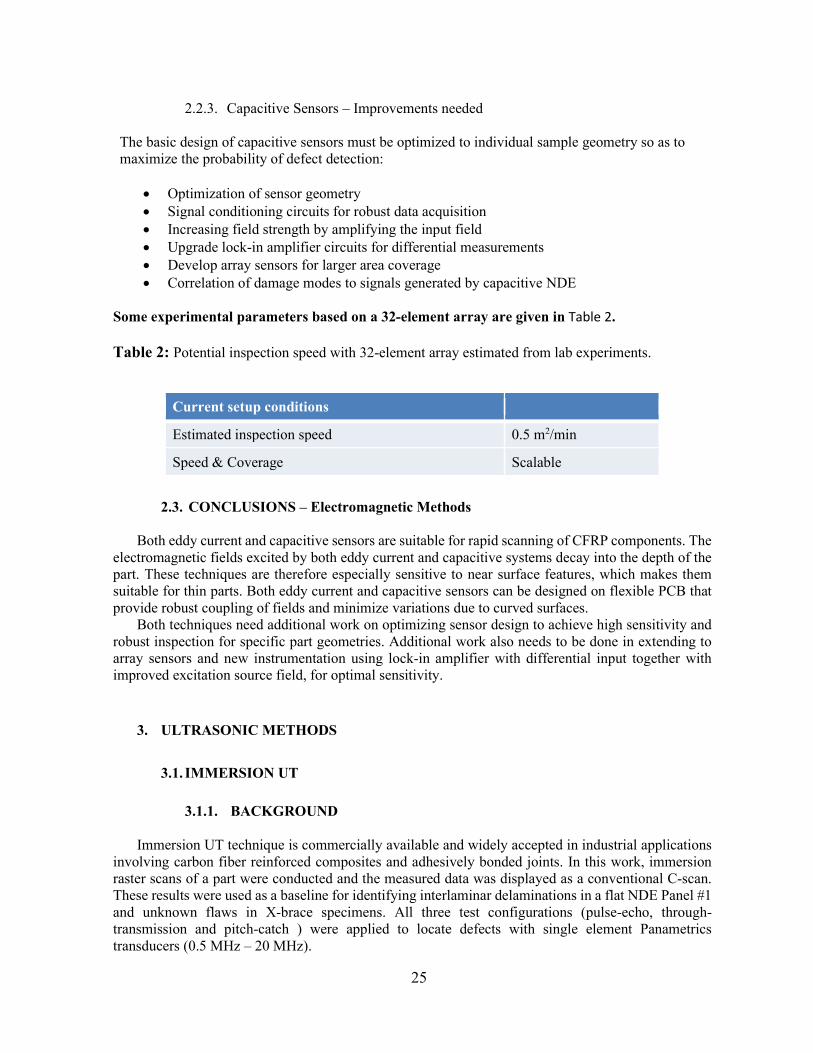
2.2.3. Capacitive Sensors – Improvements needed ........................................................ 25
2.3. CONCLUSIONS – Electromagnetic Methods ................................................................ 25 3. ULTRASONIC METHODS ........................................................................................................ 25
3.1. IMMERSION UT ............................................................................................................ 25 3.1.1. BACKGROUND ....................................................................................................... 25
3.1.2. IMMERSION UT RESULTS ON IACMI SAMPLES ..................................................... 26
3.1.2.1. Pulse-Echo mode – Panel #1 ............................................................................. 26
3.1.2.2. Pulse-Echo mode – X-Brace .............................................................................. 28
3.1.2.3. Through-Transmission mode – Panel #1 .......................................................... 32
3.1.2.4. Pitch-catch mode – Panel #1. ........................................................................... 32
3.2. AIR-COUPLED UT .......................................................................................................... 34 3.2.1. BACKGROUND ....................................................................................................... 34
3.2.2. EXPERIMENTAL SETUP .......................................................................................... 34
3.2.3 AIR COUPLED UT RESULTS ON IACMI SAMPLES.................................................... 35
3.2.4. IMPACT - Air-Coupled UT ...................................................................................... 36
3.3. GUIDED WAVE UT ......................................................................................................... 37 3.3.1. BACKGROUND ....................................................................................................... 37
3.3.2. EXPERIMENTAL SETUP .......................................................................................... 37
3.3.3. GUIDED WAVE UT RESULTS ON IACMI SAMPLES ................................................. 39
3.3.4. IMPACT Guided Wave UT ..................................................................................... 41
3.3.5. Acoustic Wave-field Imaging (AWI) ...................................................................... 41
v
3.3.6. IMPACT – Acoustic Wave Field imaging ................................................................ 42
3.3.7. IMPACT – Local Defect Resonance (LDR) .............................................................. 42
3.3.8. CONCLUSIONS- Ultrasonics ................................................................................... 42
4. SHEAROGRPAHY .................................................................................................................... 43
4.1. LASER SHEAROGRAPHY - Laser Technology, Inc ......................................................... 43 4.1.1. BACKGROUND ....................................................................................................... 43
4.1.2. EXPERIMENTAL SETUP .......................................................................................... 44
4.1.3. SHEAROGRAPHY RESULTS ON IACMI TEST SAMPLES ........................................... 44
4.1.4 Impact- Shearography Method ............................................................................. 52
4.1.5 Conclusions- Shearography ................................................................................... 53
5. INFRARED IMAGING .............................................................................................................. 53
5.1 THEMOGRAPHIC IMAGING- THERMAL WAVE IMAGING, INC .................................... 53 5.1.1 BACKGROUND .............................................................................................................. 53
5.1.2 EXPERIMENTAL SETUP .......................................................................................... 53
5.1.3 THERMOGRAPHIC IMAGING RESULTS ON IACMI TEST SAMPLES ......................... 54
5.1.4 Impact- Infrared thermography method .............................................................. 56
5.1.5 Conclusions- Thermography ................................................................................. 57
6. MICROWAVE METHOD ......................................................................................................... 57
6.1 DIELCETRIC TESTING- MWI LABS, INC .......................................................................... 57 6.1.1. BACKGROUND ....................................................................................................... 57
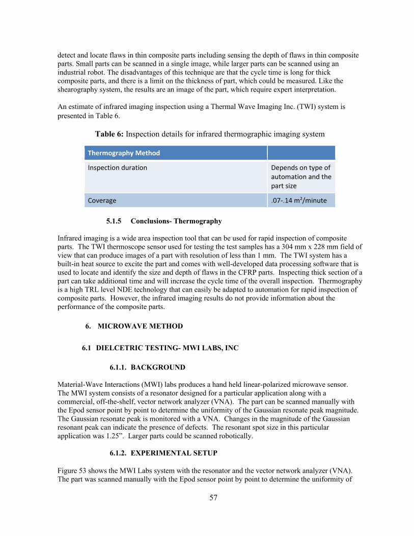
6.1.2. EXPERIMENTAL SETUP .......................................................................................... 57
6.1.3. DIELECTRIC RESULTS ON IACMI TEST SAMPLES .................................................... 58
6.1.4 Impact- Microwave Method ................................................................................. 59
7. MODAL IMPACT METHOD .................................................................................................... 60
7.1. RESONANT ACOUSTIC METHOD ....................................................................................... 60
7.1.1. BACKGROUND ............................................................................................................... 60
7.1.2. EXPERIMENTAL SETUP .................................................................................................. 60
7.1.3. RESONANT ACOUSTIC RESULTS ON IACME TEST SAMPLES .......................................... 61
7.1.4. Impacts- Resonant Acoustic Method ............................................................................ 63
8. VIBROMETRY METHOD ......................................................................................................... 63
8.1. LASER VIBROMTERY TESTING ........................................................................................... 63
8.1.1. BACKGROUND ............................................................................................................... 63
8.1.2. EXPERIMENTAL SETUP .................................................................................................. 63
8.1.3. Impacts- Laser Vibrometry ............................................................................................ 65
9. PROFILOMETRY METHOD ..................................................................................................... 65
9.1. LASER PROFILOMETRY ...................................................................................................... 65
9.1.1. BACKGROUND ............................................................................................................... 65
vi
9.1.2. EXPERIMENTAL SETUP .................................................................................................. 66
9.1.3. LASER PROFILOMETRY RESULTS ON IACMI TEST SAMPLES .......................................... 66
9.1.4. Impacts- Laser Profilometry .......................................................................................... 67
10. ULTRASONIC METHOD ...................................................................................................... 67
10.1. DRY-COUPLED MATRIX ULTRASONICS- DOLPHICAM .................................................... 67
10.1.1. BACKGORUND ............................................................................................................... 67
10.1.2. EXPERIMENTAL SETUP .................................................................................................. 67
10.1.3. DOLPHICAM RESULTS ON IACMI TEST SAMPLES .......................................................... 68
10.1.4. Impacts- Dolphicam ...................................................................................................... 71
11. Concluding Remarks ......................................................................................................... 71
12. Benefits Assessment ......................................................................................................... 74
13. Commercialization ............................................................................................................ 74
LEAD PARTNER BACKGROUND .......................................................................................................... 75
vii
LIST OF FIGURES
Figure 1: Construction details for calibration panel (Panel #1) with large (1.0”×1.0”), medium (0.5”×0.5”) and small (0.25”×0.25”) Teflon inserts. ......................................................................... 14 Figure 2: X-Brace representing complex sample geometry and unknown defects. ......................... 14 Figure 3: Composite Panel #2 (Hood corner section) representing defects in the adhesive bond-line. ................................................................................................................................................... 15 Figure 4: Composite Panel #3. .......................................................................................................... 15 Figure 5: Composite Panel #4 (Front splitter section) with embedded honeycomb structure. ....... 15 Figure 6: Composite Panel #5 (Front splitter section 2) with sandwiched honeycomb structure. .. 15 Figure 7: Experimental setup for EC testing. .................................................................................... 17 Figure 8: (a) Coil sensor, (b) CFRP sample, (c) CFRP weave pattern. ................................................ 17 Figure 9: Amplitude and phase of coil impedance at 20 MHz frequency showing punched holes in different layers. ................................................................................................................................. 18 Figure 10: Eddy current results on Panel #2. .................................................................................... 18 Figure 11: Eddy current results on Panel #4. .................................................................................... 19 Figure 12: Eddy current results on Panel #5. .................................................................................... 19 Figure 13: 3D FEM results showing electric field distribution with two sensor configurations: (a) capacitor with narrow gap, and (b) capacitor with large gap between the plates. ......................... 21 Figure 14: (a) Calibration Panel #1 , (b) scan setup for CS with the xyz-gantry. ............................... 22 Figure 15: (a) Changes in capacitance of the open-plate capacitive sensor measured in a scan of the calibration Panel #1 with Teflon inserts; (b) locations of delaminations in Panel #1. ............... 22 Figure 16: Changes in capacitance of the open-plate capacitive sensor measured in a scan of the Panel #4 . ........................................................................................................................................... 23 Figure 17: Changes in capacitance of the open-plate capacitive sensor measured in a scan of the Panel #5. ........................................................................................................................................... 24 Figure 18: Pulse-echo UT testing on Panel #1 : a) set-up (P – pulser, R - receiver); b) schematic of the test sample, scanned region is highlighted by the dotted box. ................................................. 26 Figure 19: Typical signal (A-scan) showing reflection from Teflon insert embedded in Panel #1. ... 27 Figure 20: Pulse-echo inspection results (Panel #1): a) amplitudes of reflections from Teflon inserts; b) positions of Teflon inserts across the thickness of test sample. ..................................... 28 Figure 21: Center parts of X-braces: a) image of the scanned region; b) C-Scan of X-brace #1; c) C-Scan of X-brace #2; d) C-Scans of X-brace #3. .................................................................................. 29 Figure 22: Left bottom arms of X-braces: a) image of the scanned region; b) C-Scan of X-brace #1; c) C-Scan of X-brace #2; d) C-Scan of X-brace #3. ............................................................................. 30 Figure 23: Right bottom arms of X-braces: a) image of the scanned region; b) C-Scan of X-brace #1; c) C-Scan of X-brace #2; d) C-Scans of X-brace #3. ..................................................................... 31 Figure 24: UT inspection in through-transmission mode: a) experimental set-up (T – transmitter, R - receiver); b) acquired UT C-scan. .................................................................................................... 32 Figure 25: (a) UT inspection in pitch-catch configuration; (b) pitch-catch inspection of calibration Panel #1 (T – transmitter, R - receiver). ............................................................................................ 33 Figure 26: A-Scans acquired in pitch-catch configuration. Schematic images on the right hand side show the locations where the scans were taken: (top) A-scan acquired in the healthy region; (middle) A-scan acquired at the small delamination; (bottom) A-scan acquired at the medium delamination ..................................................................................................................................... 33 Figure 27: Guided wave screening of X-braces (quick Go/No Go approach) ................................... 34 Figure 28: Experimental set-up for collecting non-contact C-scans using air-coupled transducers T (Transmitter) and R (Receiver). ......................................................................................................... 35
Figure 29: NDE Sample #1: a) top view of the sample; b) water-coupled C-scan of the region with all Teflon inserts (f = 20 MHz); c) air-coupled C-scan of the top row with three Teflon inserts (f = 300 kHz) ............................................................................................................................................ 35 Figure 30: a) Center part of X-brace #3: b) water-coupled C-scan (f = 5 MHz); c) air-coupled C-scan (f = 300 kHz, only the region with the top delamination is highlighted) .......................................... 36 Figure 31: Experimental setup with three different reflectors (surface-bonded masses). .............. 38 Figure 32: Acquired GW signals in the Path 1-2 corresponding to the presence of different surface reflectors (simulated defects). .......................................................................................................... 39 Figure 33: (a) Panel #2 with schematic view of the adherends and cross-section of the bond-line; (b) locations of piezoelectric transmitter and receivers along the bond-line. ................................. 40 Figure 34: GW signals acquired by receivers R1.b and R5.b indicating proper bonding and a disbond, respectively. ....................................................................................................................... 40 Figure 35: Bond-line monitoring results using guided wave technique. .......................................... 41 Figure 36: Acoustic wave-field imaging setup and snap shot of GW propagation. .......................... 42 Figure 37: Amplitude and phase of standing wave in Panel #1. ....................................................... 42 Figure 38: Laser Technology Inc. Shearography Measurement System ........................................... 44 Figure 39: Shearography image of Panel 1 ....................................................................................... 44 Figure 40: Shearography images measured on test sample 5 on the tool side of the part show potential wall thickness changes and potential delamination in images 2 and 3 as noted by the vendor ............................................................................................................................................... 45 Figure 41: Shearography images of three arm joints of X-brace no. 1 showing potential wall thickness changes and a possible delamination in the upper right image. ...................................... 46 Figure 42: Shearographic image measured on test sample no. 2. potentially showing resin rich areas (as noted by the vendor) ......................................................................................................... 47 Figure 43: Shearography image measured on test sample 2 that shows a potential adhesive disbond and a potential void ............................................................................................................ 48 Figure 44: Shearography image measured on test sample no. 4. that shows a potential wrinkle in the fabric of the composite part (as noted by the vendor) .............................................................. 49 Figure 45: Shearography images measured, using wrapped and unwrapped phase, on test sample 4 on the tool side of the part that shows a honeycomb edge disbond as noted by the vendor ..... 51 Figure 46: Shearography images measured on test sample no. 5. on the bag side of part that shows a potential fiber wrinkles in the composite part (as noted by the vendor) .......................... 52 Figure 47: Thermography system manufactured by Thermal Wave Imaging scanning X-Brace ...... 53 Figure 48: Thermal image measured on Panel 2 showing several anomalies at locations labeled a-e .......................................................................................................................................................... 54 Figure 49: Thermographic image of test sample 3 - no defects were noted by the vendor ............ 55 Figure 50: Thermographic images of test sample 4 - potential delaminations were noted by the vendor around machined holes ........................................................................................................ 56 Figure 51: Thermographic image of test sample 5 - no flaws were noted by the vendor ............... 56 Figure 52: MWI system that consists of a resonator designed for a particular application along with a commercial off-the-shelf vector network analyzer (VNA). .................................................... 58 Figure 53: Reference locations assigned to the part and the locations of the defects .................... 58 Figure 54: Modal Shop automated / semi-automated systems ....................................................... 60 Figure 55: Test set up with the microphone and the accelerometers used to conduct the modal impact tests on the three (3) sample X-braces ................................................................................. 61 Figure 56: Example of an impact force and microphone response signal ........................................ 61 Figure 57: Comparison of microphone and accelerometer FRFs on X-brace test sample ............... 62 Figure 58: FRF’s measured with a ½” microphone on the three (3) X-braces .................................. 62
ix
Figure 59: Scanning laser vibrometer setup showing test configuration for Panel 5 ....................... 64 Figure 60: Frequency response functions for Panel 5 using scanning laser vibrometer .................. 64 Figure 61: Measured operating deflection shapes for Panel 5 using laser vibrometer ................... 65 Figure 62: Laser profilometers manufactured by Keyence ............................................................... 66 Figure 63: Test setup for measuring Panel 1 with the laser profilometer ........................................ 66 Figure 64: Laser profilometry test results ......................................................................................... 67 Figure 65: Dolphicam sensor being used to test Panel 1 .................................................................. 68 Figure 66: location of know defects in the calibration panel no. 1 .................................................. 68 Figure 67: Dolphicam measurement results on Panel 1- defects in bottom layer ........................... 69 Figure 68: Dolphicam measurement results on Panel 1- defects in middle layer ............................ 69 Figure 69: Dolphicam measurement results on Panel 1- defects in top layer .................................. 70 Figure 70: Dolphicam measurement results on Panel 3- anomaly circled in red ............................. 70 Figure 71: Dolphicam measurement results on Panel 4 ................................................................... 71
LIST OF TABLES Table 1: Inspection speed conditions during initial lab tests as presented in this report….………….. 18 Table 2: Potential inspection speed with a 32 element array estimated from lab experiment….…. 23 Table 3: Potential inspection speed estimated from lab experiments……………………………... 32 Table 4: Potential inspection speed estimated from lab experiments……………………………... 34 Table 5: Inspection details for laser shearography system………………………………………... 46 Table 6: Inspection details for infrared thermographic imaging system………………………….. 50 Table 7: Test data from MWI labs hand held linear-polarized microwave sensor- highlighted test data shown shows the locations of the defects in Panel 1…………………………………………. 52 Table 8: Inspection details for MWI Labs microwave method…………………………………… 53 Table 9: Inspection details for resonant acoustic method…………………………………………. 56 Table 10: Inspection details for 3D laser vibrometry……………………………………….…….. 58 Table 11: Summary of NDE technologies investigated…………………………………………… 65 Table 12: Summary of rated metrics shown for each NDE technology……………………...…… 66 Table 13: Summary of rated metrics shown for each NDE technology…………………………... 67 Table 14: Overall ratings determined for each of the remaining NDE technologies…………....… 67
LIST OF ACRONYMS 3D- 3 Dimensional ACUT- Air Coupled Ultrasonic Testing ACC- American Chemistry Council A-SCAN- Amplitude scan, acquired ultrasonic signal. AWI- Acoustic Wave-field Imaging B-SCAN- array of A-scans CAPX- Capital Expenditures CI- Capacitive Imaging CFRP- Carbon Fiber Reinforced Polymer C-SCAN- image constructed from multiple A-scans, a plan-type view of inspected sample. dB-Decibels EC- Eddy Current EERE- Energy Efficiency and Renewable Energy FEM- Finite Element Method FOD- Foreign Object Debris
FOV- Field of View FRF- Frequency Response Function GFRP- Glass Fiber Reinforced Polymer GW- Guided Waves EC- Eddy Current Hz- Hertz IACMI – Institute for Advanced Composites Manufacturing Innovation IR- Infrared LDR- Local Defect Resonance LDV- Laser Doppler Vibrometer LTI- Laser Technology, Inc. MWI- Material Wave Interactions NDE- Nondestructive Evaluation NDT- Nondestructive Testing P- Pulser PCB- Printed Circuit Board (PCB) R- Receiver RTM- Resin Transfer Molding SLDV- Scanning Laser Doppler Vibrometer SNR-Signal to Noise Ratio STD- standard T- Transmitter TOF- Time of Flight TSR- Thermographic Signal Reconstruction TWI- Thermal Wave Imaging, Inc UT- Ultrasonic Testing VNA- Vector Network Analyzer

ix
ACKNOWLEDGEMENTS
The information, data, or work presented herein was funded in part by the Office of Energy Efficiency and Renewable Energy (EERE), U.S. Department of Energy, under Award DE- EE0006926 with the Institute for Advanced Composites Manufacturing Innovation (IACMI).
12
EXECUTIVE SUMMARY
Current composite inspection technologies are tailored towards low-volume, high value parts. The needs and priorities for high-volume mainstream automotive production are very different from those of aerospace or similar sectors that have adopted advanced composite materials at scale. Beyond efficacy, the priority for inspection in the automotive sector is a short cycle time, which does not inhibit the rate of production. The target cycle time per part is 3 minutes, with a stretch goal of 1 minute. This report details the evaluation approach, the technologies of interest, and the performance of a number of inspection technologies applied to automotive carbon fiber composites.
1. INTRODUCTION Rapid, cost-effective non-destructive inspection is necessary to drive the wide scale adoption of
advanced composites in the automotive sector. There are both technical and business-related drivers for this need. There is a technical need for effective inspection that can improve process control and reduce variation in the manufacturing process, and thereby enable lighter, less conservative designs, and a reduction in scrap. Manufacturers in the automotive sector are necessarily cautious regarding new materials. Risks of legal liabilities for warranty of structural automotive composites are a significant concern throughout the supply chain need to be managed which could present a hurdle to wider adoption of advanced composite materials. These risks could be greatly reduced by implementing an endpoint inspection of every part that comes off the manufacturing line. The endpoint inspection method selected needs to group or classify the composite parts based on geometry and performance requirements of the composite part
The objective of Phase I has been to evaluate NDE technologies for high volume automotive composite parts. To this end, existing automotive composite parts manufactured by Plasan Composites were provided to evaluate several NDE technologies on representative testbeds. Among those parts were three X-braces for a Dodge Viper, one composite calibration plaque with known defects at know locations, and four other test sections, including sections from a front splitter, a corner section from a composite hood and a high pressure RTM panel made using non crimp fabric.
Using these composite parts, several NDE technologies were evaluated by Vanderbilt University and Michigan State University. The test results and analyses were reviewed by the team to evaluate the efficacy of each method in identifying defects in the test parts. The project management team consisting of Dale Brosius from IACMI, Suzanne Cole and Gina Oliver from ACC, and Doug Bradley from Plasan Composites ranked the NDE technologies and reviewed the results with the NDE Project Peer Review Panel. The project review panel was made up of Diane Chinn from Lawrence Livermore National Laboratory, Nicholas Gianaris from Thermacore, Golam Newaz from Wayne State University, Eric Lindgren from US Air Force Materials Laboratory, Francesco Lanza DiScalea from UC San Diego, and Laurence Jacobs from Georgia Institute of Technology. The review panel identified the NDE technologies that showed the highest potential to effectively screen the composite part in the requisite cycle time for further development in Phase II.
The project management team down select 2-4 of the NDE technologies evaluated that show highest potential to group or classify the composite parts based on geometry and performance requirements of the composite part, meet the 3 minute cycle time target and the stretch goal of a 1 minute cycle time for further development in Phase II.
13
NDE Technologies Evaluated in Phase I
A number of NDE technologies were evaluated with an eye towards scalability and suitability in an industrial environment. Each technology was tested on the same set of parts where possible to allow for direct comparison.
• Electromagnetic methods o Eddy Current Testing (EC) o Capacitive Imaging (CI)
• Ultrasonic methods o Guided wave UT o Wave field imaging o Immersion UT
Pulse-Echo Through transmission Pitch-catch
o Air coupled UT • Infrared Imaging - Thermal Wave Imaging • Material Wave Interactions - MWI Labs • Laser Shearography - Laser Technology, Inc. • Infrared Imaging - Thermal Wave Imaging • Modal Impact Testing/Resonant Acoustic Method • Laser Profilometry • Laser Vibrometry • Dolphicam (Matrix Ultrasonic)
Each NDE technology was evaluated by the ACC 3.8 project management team based on inspection speed, coverage area, industrial durability, detection accuracy, and versatility of the inspection data. Potential flaws of interest included delaminations, cracks, porosity (a cluster of voids), missing plies, mis-oriented plies, ply drops, misplacement of slits/darts, reinforcement wrinkles, foreign object debris, machining damage, and resin rich or resin lean areas. In addition, the ability of each technology to quickly inform a decision making process was important to the project objectives, so the ability of techniques to classify parts based on the presence of defects or manufacturing error was important. Composite Parts used for the Evaluation of NDE Technologies
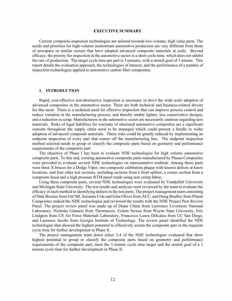
A flat stepped carbon fiber epoxy laminate was provided as calibration standard that contained defects with specified sizes that were inserted between specific plies. Figure 1 shows the defect layout of calibration panel number 1. The calibration standard sample was used to evaluate the detection sensitivity and resolution of the NDI technique. No attempt was made to characterize the root cause or classify the defect into the types listed above.
14
Figure 1: Construction details for calibration panel (Panel #1) with large (1.0”×1.0”), medium (0.5”×0.5”) and small (0.25”×0.25”) Teflon inserts.
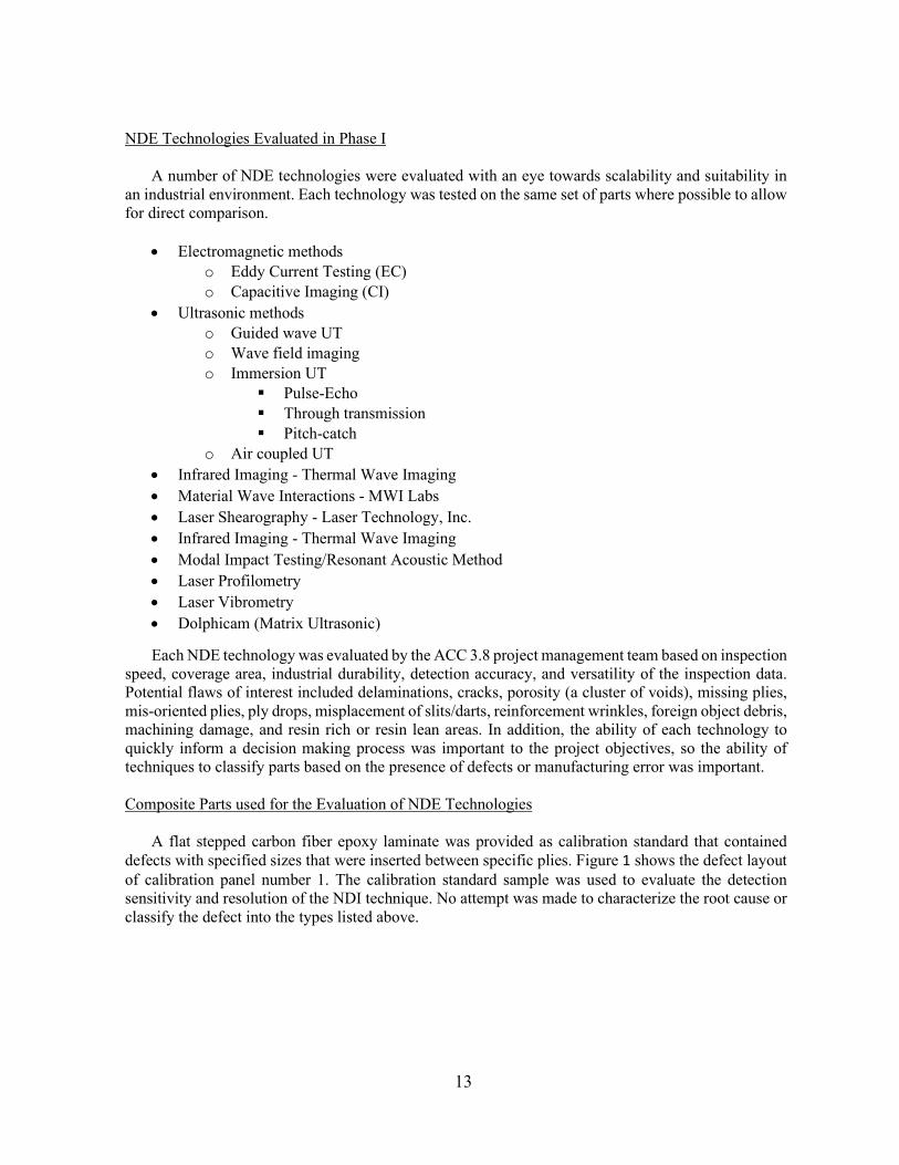
Figure 2 - Figure 6 show pictures of the composite parts that were provided to evaluate the NDE technologies listed above. These parts provide a good variety of part thickness and material selections, with some honeycomb sandwich parts, parts with adhesively bonded joints, and parts with machined holes. These features are of interest in the final application, so the ability to test these techniques on realistic parts has been valuable.
Figure 2: X-Brace representing complex sample geometry and unknown defects.

15
Figure 3: Composite Panel #2 (Hood corner section) representing defects in the adhesive bond-line.
Figure 4: Composite Panel #3.
Figure 5: Composite Panel #4 (Front splitter section) with embedded honeycomb structure.
Figure 6: Composite Panel #5 (Front splitter section 2) with sandwiched honeycomb structure.
16
2. ELECTROMAGNETIC METHODS
2.1. EDDY CURRENT
2.1.1. BACKGROUND
Eddy current (EC) testing is a mature technology that has become standard in many industrial applications. Eddy current (EC) inspection techniques are non-contact, rapid and low-cost. However, existing commercial equipment and off-the-shelf probes are mostly optimized for detection of defects in metals. Application of EC techniques for inspection of CFRP structures shows promise. Detection of different types of defects that affect local conductivity of a sample, such as fiber breakage and waviness has been demonstrated [1]. Development of EC sensors for rapid NDI of CFRP automotive parts is challenging owing to low conductivity of CFRP, electrical anisotropy of CFRP, complex shapes of parts and multiple damage types. Thus, flexible array sensors with ability to operate at MHz frequencies need to be designed and fabricated.
Equation (1) shows the conductivity tensor 𝜎𝜎� of a unidirectional CFRP ply with fibers in x-y plane:
𝜎𝜎� = �𝜎𝜎𝐿𝐿𝑐𝑐𝑐𝑐𝑐𝑐2𝜃𝜃 + 𝜎𝜎𝑇𝑇𝑐𝑐𝑠𝑠𝑠𝑠2𝜃𝜃 (𝜎𝜎𝐿𝐿 − 𝜎𝜎𝑇𝑇)𝑐𝑐𝑠𝑠𝑠𝑠𝜃𝜃𝑐𝑐𝑐𝑐𝑐𝑐𝜃𝜃 0(𝜎𝜎𝐿𝐿 − 𝜎𝜎𝑇𝑇)𝑐𝑐𝑠𝑠𝑠𝑠𝜃𝜃𝑐𝑐𝑐𝑐𝑐𝑐𝜃𝜃 𝜎𝜎𝐿𝐿𝑐𝑐𝑠𝑠𝑠𝑠2𝜃𝜃 + 𝜎𝜎𝑇𝑇𝑐𝑐𝑐𝑐𝑐𝑐2𝜃𝜃 0
0 0 𝜎𝜎𝑐𝑐𝑐𝑐�, (1)
where 𝜎𝜎𝐿𝐿 and 𝜎𝜎𝑇𝑇 are the conductivities in the fiber direction and transverse direction respectively, and 𝜎𝜎𝑐𝑐𝑐𝑐 is the cross ply conductivity, 𝜃𝜃 is the fiber orientation with respect to the x axis. Typically, 𝜎𝜎𝐿𝐿 usually lies between 5 × 10³ and 5 × 10⁴ S/m. Typical values of 𝜎𝜎𝑇𝑇 and 𝜎𝜎𝑐𝑐𝑐𝑐 are between 1 and 100 S/m. As the conductivity of carbon fiber is much lower than metal, a higher excitation frequency is needed. It is also important to optimize the sensor/coil design in order to induce currents that produce a strong interaction with defects of different types [2,3]. [1] Cheng J., Qui J., Xu X., Ji H., Takagi T. and Uchimoto T. “Research Advances in Eddy Current
Testing for Maintenance of Carbon Fiber Reinforced Plastic Composites”, International Journal of Applied Electromagnetics and Mechanics, 51(3), p. 261, 2016.
[2] Ye C., Udpa L. and Udpa, S.S. “Optimization and Validation of Rotating Current Excitation with GMR Array Sensors for Riveted Structures Inspection”, Sensors (Basel), 16(9), p. 1512, 2016.
[3] Rosell, A. Ye C., Krishna V., Karpenko O., Tamburrino A., Forestiere C., Udpa L., Udpa S.S., Rubinacci G., Ventre S., “Electromagnetic NDT of Composite Materials: Experimental Tests and Numerical Models”, CAMX 2016, Anaheim, CA.
2.1.2. EXPERIMENTAL SETUP
The eddy current sensor was mounted on a holder in the xyz-gantry to facilitate the scanning procedure. The excitation current was produced using a waveform generator (Agilent 35500B). The signal was captured using a lock-in amplifier model 844 from Stanford research systems which has a frequency range of 25 kHz to 200 MHz. Data was collected with a single sensor element in a raster scan with well-defined resolution along both x and y axis at a speed of 20 mm/s. The overall experimental configuration is shown in Figure 7.
17
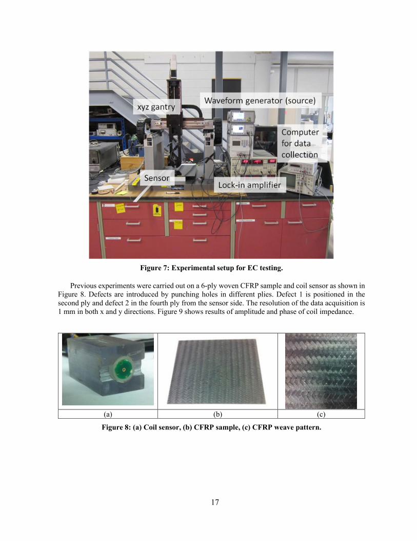
Figure 7: Experimental setup for EC testing.
Previous experiments were carried out on a 6-ply woven CFRP sample and coil sensor as shown in
Figure 8. Defects are introduced by punching holes in different plies. Defect 1 is positioned in the second ply and defect 2 in the fourth ply from the sensor side. The resolution of the data acquisition is 1 mm in both x and y directions. Figure 9 shows results of amplitude and phase of coil impedance.
(a) (b) (c)
Figure 8: (a) Coil sensor, (b) CFRP sample, (c) CFRP weave pattern.

18
(a) (b)
Figure 9: Amplitude and phase of coil impedance at 20 MHz frequency showing punched holes in different layers.
Defects such as fiber breakage that interrupts current path can be detected with high accuracy using eddy current probes. However, delaminations that alter the z-directional conductivity without altering eddy current path in the x-y plan (Panel #1 with thin Teflon inserts) are not been detected with simple coil probes and may need new coil designs.
2.1.3. EC COIL SENSOR RESULTS ON IACMI SAMPLES
As the xyz-gantry was able to scan only flat samples, only selected surfaces on Panels #2, #4 and #5 were scanned. These results are presented in Figure 10 to Figure 12 below.
1. Subsurface feature
2. Scan of the adhesive bond-line from the far side
Figure 10: Eddy current results on Panel #2.
19
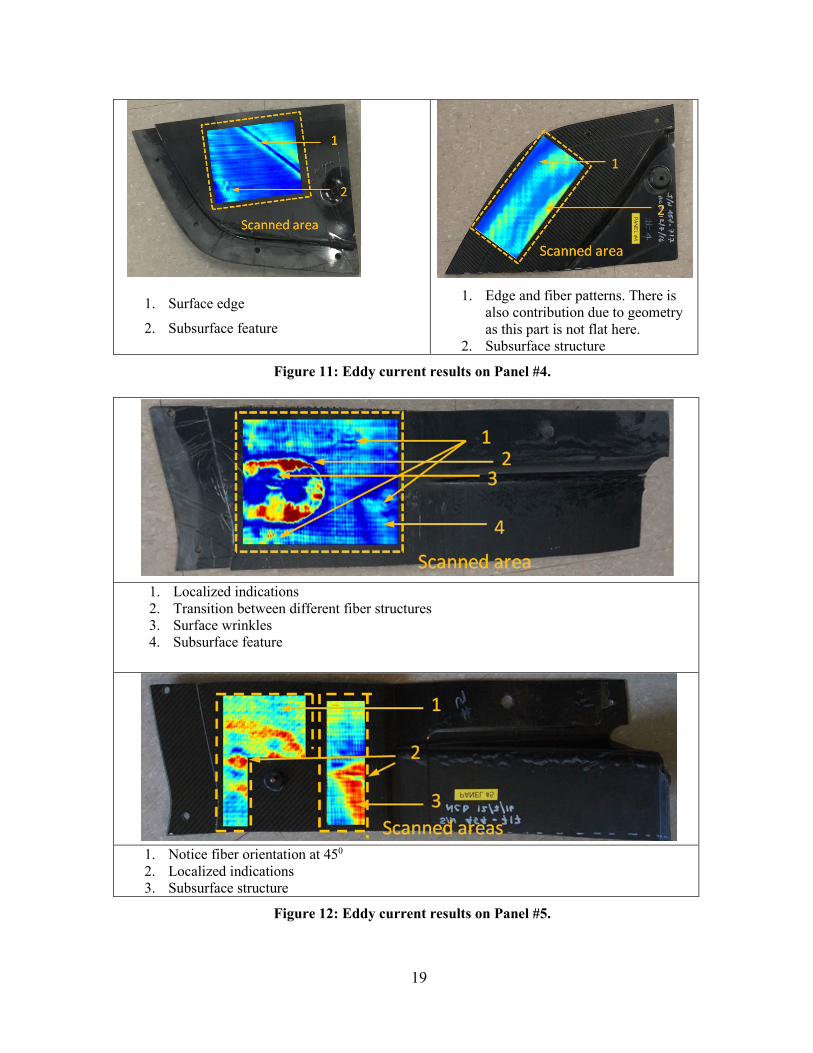
1. Surface edge
2. Subsurface feature
1. Edge and fiber patterns. There is
also contribution due to geometry as this part is not flat here.
2. Subsurface structure
Figure 11: Eddy current results on Panel #4.
1. Localized indications 2. Transition between different fiber structures 3. Surface wrinkles 4. Subsurface feature
1. Notice fiber orientation at 450 2. Localized indications 3. Subsurface structure
Figure 12: Eddy current results on Panel #5.

20
2.1.4. Eddy Current Sensors – Improvements Needed
The basic eddy current sensor system has to be tailored to individual sample geometry. In the current application the following improvements are needed for maximizing the probability of detection:
• Develop efficient and flexible design of eddy current array sensors and instrumentation for larger area coverage.
• Optimization of excitation coil geometry and pick up sensors. • Development of signal processing tools for accurate CFRP integrity evaluation based on
eddy current data. Some experimental parameters based on a 32-element array sensor are presented in Table 1.
Table 1: Estimated parameters of a 32-element coil probe based on initial lab tests as presented in the report.
Current setup (32-element array)
Estimated inspection speed 0.5 m2/min
Speed & Coverage Scalable
2.2. CAPACITIVE SENSING
2.2.1. BACKGROUND
The overall principle of capacitive sensing (CS) relies on measurement of local changes in capacitance of the test sample, which depends on the dielectric properties of the material and presence of defects. Capacitive sensors can be used to detect multiple damage types in carbon and glass fiber reinforced polymers. The method offers flexible NDE with non-contact low cost sensors which can be built into array systems and used for rapid scanning of large parts.
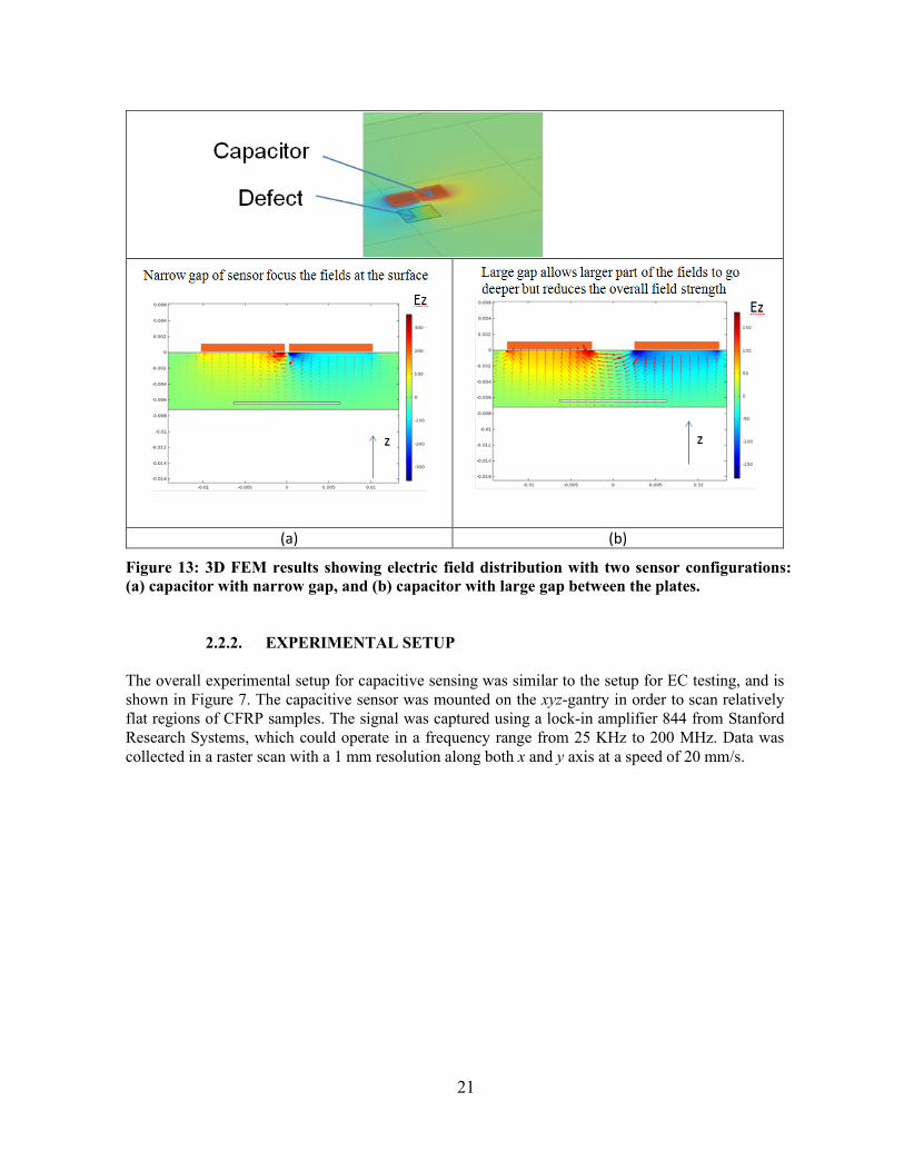
A capacitive sensor produces strong electric field in the direction normal to the surface of the test sample. Usually, CFRP samples have low conductivity along this direction. Hence, the electric field can penetrate the sample, and changes in electrical properties such as permittivity or conductivity will alter the measured capacitance. Since the fields are closely localized, the geometry of the capacitive sensor is critical in determining the sensitivity to defect size and depth as seen in the simulation results in Figure 13. Capacitive sensors are therefore suitable for thin structures and are in general more sensitive to surface and near-surface defects.
21
(a) (b)
Figure 13: 3D FEM results showing electric field distribution with two sensor configurations: (a) capacitor with narrow gap, and (b) capacitor with large gap between the plates.
2.2.2. EXPERIMENTAL SETUP
The overall experimental setup for capacitive sensing was similar to the setup for EC testing, and is shown in Figure 7. The capacitive sensor was mounted on the xyz-gantry in order to scan relatively flat regions of CFRP samples. The signal was captured using a lock-in amplifier 844 from Stanford Research Systems, which could operate in a frequency range from 25 KHz to 200 MHz. Data was collected in a raster scan with a 1 mm resolution along both x and y axis at a speed of 20 mm/s.
22
CAPACITIVE SENSOR RESULTS ON IACMI SAMPLES
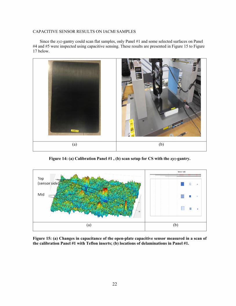
Since the xyz-gantry could scan flat samples, only Panel #1 and some selected surfaces on Panel #4 and #5 were inspected using capacitive sensing. These results are presented in Figure 15 to Figure 17 below.
(a) (b)
Figure 14: (a) Calibration Panel #1 , (b) scan setup for CS with the xyz-gantry.
(a) (b)
Figure 15: (a) Changes in capacitance of the open-plate capacitive sensor measured in a scan of the calibration Panel #1 with Teflon inserts; (b) locations of delaminations in Panel #1.

23
Measurement using capacitor with higher sensitivity close to scanning surface (narrow gap as in Figure 13a)
1. Subsurface features
Measurement using capacitor with deeper penetration of electric field (large gap as in Figure 13b)
1. Subsurface
features
Figure 16: Changes in capacitance of the open-plate capacitive sensor measured in a scan of the Panel #4 .

24
Results using capacitor with higher sensitivity close to the surface (narrow gap)
1. Tape on the surface (put there to avoid sensor from hitting edges of the holes) 2. Wrinkles on the surface of the part 3. Variation in fiber structure 4. Internal structure
Results using capacitor with deeper penetration of fields (large gap)
1. Localized indication 2. Internal structure
Results from capacitor design with higher sensitivity close to the surface
1. Localized indication
Figure 17: Changes in capacitance of the open-plate capacitive sensor measured in a scan of the Panel #5.
25
2.2.3. Capacitive Sensors – Improvements needed The basic design of capacitive sensors must be optimized to individual sample geometry so as to maximize the probability of defect detection:
• Optimization of sensor geometry • Signal conditioning circuits for robust data acquisition • Increasing field strength by amplifying the input field • Upgrade lock-in amplifier circuits for differential measurements • Develop array sensors for larger area coverage • Correlation of damage modes to signals generated by capacitive NDE
Some experimental parameters based on a 32-element array are given in Table 2. Table 2: Potential inspection speed with 32-element array estimated from lab experiments.
Current setup conditions
Estimated inspection speed 0.5 m2/min
Speed & Coverage Scalable
2.3. CONCLUSIONS – Electromagnetic Methods
Both eddy current and capacitive sensors are suitable for rapid scanning of CFRP components. The electromagnetic fields excited by both eddy current and capacitive systems decay into the depth of the part. These techniques are therefore especially sensitive to near surface features, which makes them suitable for thin parts. Both eddy current and capacitive sensors can be designed on flexible PCB that provide robust coupling of fields and minimize variations due to curved surfaces.
Both techniques need additional work on optimizing sensor design to achieve high sensitivity and robust inspection for specific part geometries. Additional work also needs to be done in extending to array sensors and new instrumentation using lock-in amplifier with differential input together with improved excitation source field, for optimal sensitivity.
3. ULTRASONIC METHODS 3.1. IMMERSION UT
3.1.1. BACKGROUND
Immersion UT technique is commercially available and widely accepted in industrial applications
involving carbon fiber reinforced composites and adhesively bonded joints. In this work, immersion raster scans of a part were conducted and the measured data was displayed as a conventional C-scan. These results were used as a baseline for identifying interlaminar delaminations in a flat NDE Panel #1 and unknown flaws in X-brace specimens. All three test configurations (pulse-echo, through-transmission and pitch-catch ) were applied to locate defects with single element Panametrics transducers (0.5 MHz – 20 MHz).
26
3.1.2. IMMERSION UT RESULTS ON IACMI SAMPLES
3.1.2.1. Pulse-Echo mode – Panel #1
A single transducer is used for NDI in pulse-echo UT. The transducer is first driven by a few high voltage pulses in order to generate the ultrasonic waves, and after that it is switched into a receiving mode in order to acquire resulting signals. Wave excitation is performed at normal incidence with respect to top surface of the sample. UT waves penetrate into the specimen through coupling medium such as water for better acoustic impedance matching. Signals acquired by the transducer (amplitude A-scans) show wave reflections from interfaces such as top and bottom walls of the sample. The presence of defects in the sample affects the measurements by either introducing additional reflections (e.g. interlaminar delamination) or attenuation owing to wave scattering (e.g. agglomeration of air voids, matrix cracking). Test sample is inspected using 2D raster scanning, and an ultrasonic signal (A-Scan) is acquired at every scan position. A-Scans can be filtered or averaged in order to reduce measurement noise. After that, a single feature is selected from each A-scan (for instance, peak amplitude, energy or time-of-flight), and it is plotted on a corresponding pixel of a 2D grid, thus forming a 3D representation of ultrasonic data, or a C-scan. Analyzing A-scans in different time gates helps identify depth of defects or structural features.
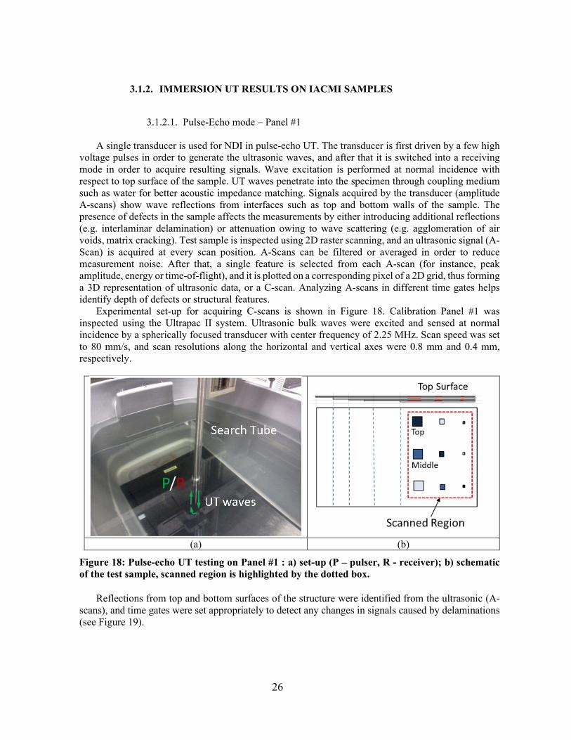
Experimental set-up for acquiring C-scans is shown in Figure 18. Calibration Panel #1 was inspected using the Ultrapac II system. Ultrasonic bulk waves were excited and sensed at normal incidence by a spherically focused transducer with center frequency of 2.25 MHz. Scan speed was set to 80 mm/s, and scan resolutions along the horizontal and vertical axes were 0.8 mm and 0.4 mm, respectively.
(a) (b)
Figure 18: Pulse-echo UT testing on Panel #1 : a) set-up (P – pulser, R - receiver); b) schematic of the test sample, scanned region is highlighted by the dotted box.
Reflections from top and bottom surfaces of the structure were identified from the ultrasonic (A-scans), and time gates were set appropriately to detect any changes in signals caused by delaminations (see Figure 19).
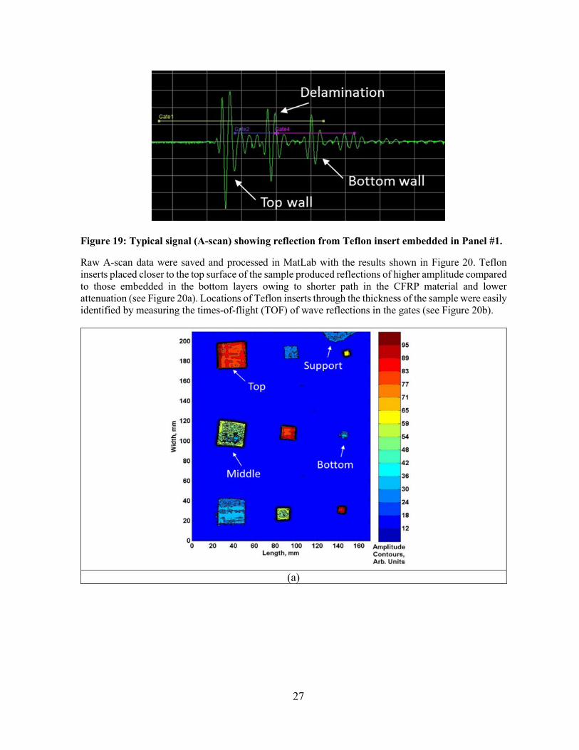
27
Figure 19: Typical signal (A-scan) showing reflection from Teflon insert embedded in Panel #1.
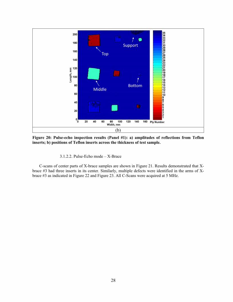
Raw A-scan data were saved and processed in MatLab with the results shown in Figure 20. Teflon inserts placed closer to the top surface of the sample produced reflections of higher amplitude compared to those embedded in the bottom layers owing to shorter path in the CFRP material and lower attenuation (see Figure 20a). Locations of Teflon inserts through the thickness of the sample were easily identified by measuring the times-of-flight (TOF) of wave reflections in the gates (see Figure 20b).
(a)
28
(b)
Figure 20: Pulse-echo inspection results (Panel #1): a) amplitudes of reflections from Teflon inserts; b) positions of Teflon inserts across the thickness of test sample.
3.1.2.2. Pulse-Echo mode – X-Brace
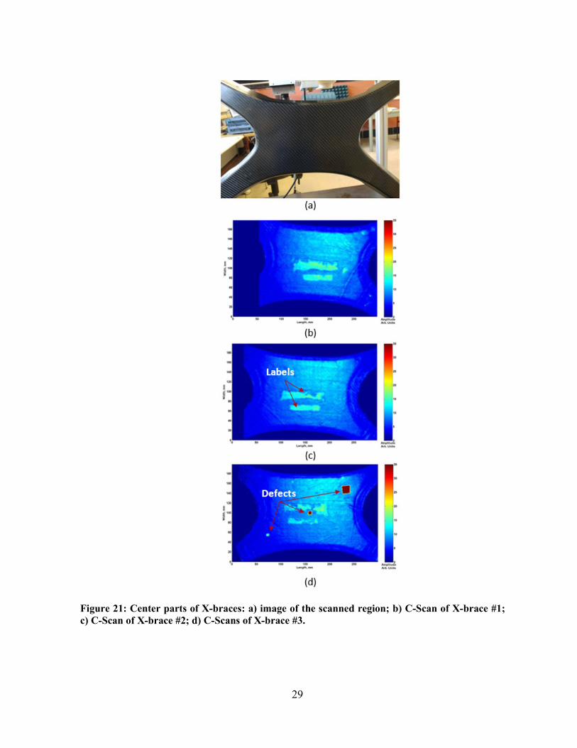
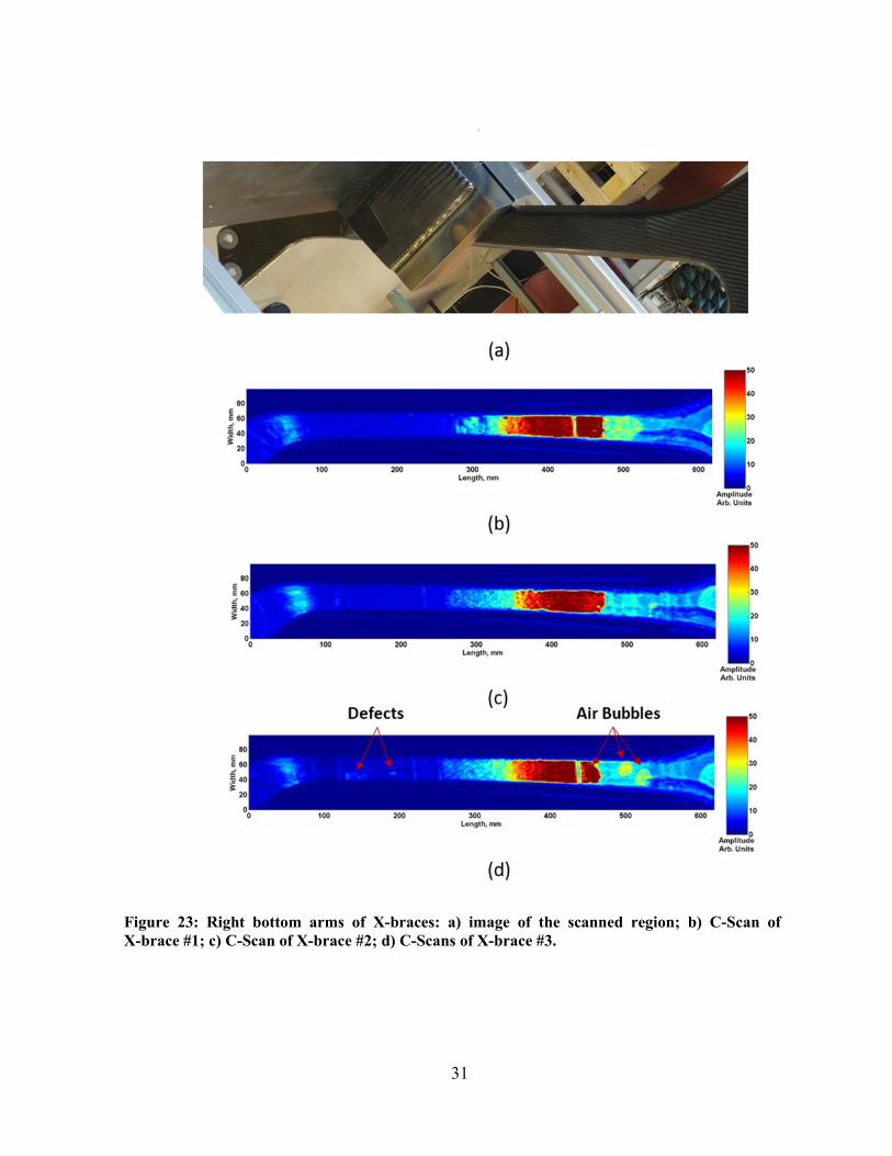
C-scans of center parts of X-brace samples are shown in Figure 21. Results demonstrated that X-brace #3 had three inserts in its center. Similarly, multiple defects were identified in the arms of X-brace #3 as indicated in Figure 22 and Figure 23. All C-Scans were acquired at 5 MHz.
29
Figure 21: Center parts of X-braces: a) image of the scanned region; b) C-Scan of X-brace #1; c) C-Scan of X-brace #2; d) C-Scans of X-brace #3.

30
Figure 22: Left bottom arms of X-braces: a) image of the scanned region; b) C-Scan of X-brace #1; c) C-Scan of X-brace #2; d) C-Scan of X-brace #3.
31
Figure 23: Right bottom arms of X-braces: a) image of the scanned region; b) C-Scan of X-brace #1; c) C-Scan of X-brace #2; d) C-Scans of X-brace #3.
32
3.1.2.3. Through-Transmission mode – Panel #1
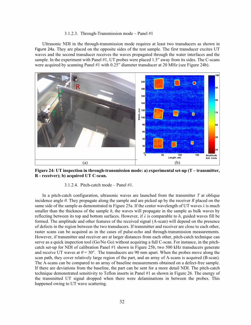
Ultrasonic NDI in the through-transmission mode requires at least two transducers as shown in Figure 24a. They are placed on the opposite sides of the test sample. The first transducer excites UT waves and the second transducer receives the waves propagated through the water interfaces and the sample. In the experiment with Panel #1, UT probes were placed 1.5” away from its sides. The C-scans were acquired by scanning Panel #1 with 0.25” diameter transducer at 20 MHz (see Figure 24b).
(a) (b)
Figure 24: UT inspection in through-transmission mode: a) experimental set-up (T – transmitter, R - receiver); b) acquired UT C-scan.
3.1.2.4. Pitch-catch mode – Panel #1.
In a pitch-catch configuration, ultrasonic waves are launched from the transmitter T at oblique incidence angle θ. They propagate along the sample and are picked up by the receiver R placed on the same side of the sample as demonstrated in Figure 25a. If the center wavelength of UT waves λ is much smaller than the thickness of the sample h, the waves will propagate in the sample as bulk waves by reflecting between its top and bottom surfaces. However, if λ is comparable to h, guided waves fill be formed. The amplitude and other features of the received signal (A-scan) will depend on the presence of defects in the region between the two transducers. If transmitter and receiver are close to each other, raster scans can be acquired as in the cases of pulse-echo and through-transmission measurements. However, if transmitter and receiver are at larger distances from each other, pitch-catch technique can serve as a quick inspection tool (Go/No Go) without acquiring a full C-scan. For instance, in the pitch-catch set-up for NDI of calibration Panel #1 shown in Figure 25b, two 500 kHz transducers generate and receive UT waves at θ = 30°. The transducers are 90 mm apart. When the probes move along the scan path, they cover relatively large region of the part, and an array of A-scans is acquired (B-scan). The A-scans can be compared to an array of baseline measurements obtained on a defect-free sample. If there are deviations from the baseline, the part can be sent for a more detail NDI. The pitch-catch technique demonstrated sensitivity to Teflon inserts in Panel #1 as shown in Figure 26. The energy of the transmitted UT signal dropped when there were delaminations in between the probes. This happened owing to UT wave scattering.

33
(a) (b)
Figure 25: (a) UT inspection in pitch-catch configuration; (b) pitch-catch inspection of calibration Panel #1 (T – transmitter, R - receiver).
Figure 26: A-Scans acquired in pitch-catch configuration. Schematic images on the right hand side show the locations where the scans were taken: (top) A-scan acquired in the healthy region; (middle) A-scan acquired at the small delamination; (bottom) A-scan acquired at the medium delamination

34
Potential approach for UT screening of X-brace arms (Go/No Go) is presented in Figure 27. Guided waves will propagate from one side of the part to another. In this case a set of B-scans will be taken along the scan path and compared to a baseline.
Figure 27: Guided wave screening of X-braces (quick Go/No Go approach)
Pitch-catch inspection offers high scanning speed due to broader coverage. This estimation based on a 2” distance between the transducers is provided in Table 3.
Table 3: Potential inspection speed estimated from lab experiments
Setup conditions 2” distance between the transducers
Estimated inspection speed >0.38 m2/min
Inspection speed & Coverage Depend on the distance between UT probes
3.2. AIR-COUPLED UT
3.2.1. BACKGROUND
Recently, air-coupled ultrasonic techniques have emerged as a viable tool for characterization and
non-destructive evaluation of composite materials using bulk waves and guided waves. Excluding couplants between the transducer and the structure can be very advantageous in industrial environment, since this simplifies handling of components during the inspection. However, application of non-contact piezoelectric transducers is limited by the big losses of ultrasonic signals due to attenuation and mismatch of the acoustic impedances. One of the ways to alleviate this problem is by application of novel piezoelectric materials and impedance matching layers for improved acoustic coupling. In Phase I of the project, we tested the state-of-the-art air-coupled UT transducers provided by Sonotec for rapid NDE of CFRP test specimens.
3.2.2. EXPERIMENTAL SETUP
Experimental set-up for Air coupled UT is shown Figure 28. A pair of flat-bottom CF-300 transducers with a center frequency of 300 kHz was operated in a through-transmission mode to exclude the effects of strong reflections from the top surfaces of inspected samples. Transducers were mounted on custom fabricated fixtures. Signals sensed by the receiving transducer were amplified with a broadband 60 dB pre-amplifier 2/4/6C (Physical Acoustics Corporation). Second-stage 80 dB gain was added by the pulser-receiver board of the Ultrapac II system. The scan speed was set to 80 mm/s, and 4 averages were taken per A-scan. C-scans were then formed by computing the averaged energy of acoustic pulses transmitted through the sample.

35
Figure 28: Experimental set-up for collecting non-contact C-scans using air-coupled
transducers T (Transmitter) and R (Receiver).
3.2.3 AIR COUPLED UT RESULTS ON IACMI SAMPLES
Air-coupled C-scan of the NDE Panel #1 is shown in Figure 29c. Results demonstrated that the Teflon inserts could be successfully detected.
Figure 29: NDE Sample #1: a) top view of the sample; b) water-coupled C-scan of the region with all Teflon inserts (f = 20 MHz); c) air-coupled C-scan of the top row with three Teflon inserts (f = 300 kHz)
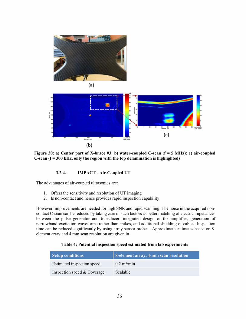
Non-contact C-scan the X-brace #3 is demonstrated in Figure 30c. Upper right part of the center region was scanned, and the largest defect was successfully detected as in the case of the immersion test.
36
Figure 30: a) Center part of X-brace #3: b) water-coupled C-scan (f = 5 MHz); c) air-coupled C-scan (f = 300 kHz, only the region with the top delamination is highlighted)
3.2.4. IMPACT - Air-Coupled UT
The advantages of air-coupled ultrasonics are:
1. Offers the sensitivity and resolution of UT imaging 2. Is non-contact and hence provides rapid inspection capability
However, improvements are needed for high SNR and rapid scanning. The noise in the acquired non-contact C-scan can be reduced by taking care of such factors as better matching of electric impedances between the pulse generator and transducer, integrated design of the amplifier, generation of narrowband excitation waveforms rather than spikes, and additional shielding of cables. Inspection time can be reduced significantly by using array sensor probes. Approximate estimates based on 8-element array and 4 mm scan resolution are given in
Table 4: Potential inspection speed estimated from lab experiments
Setup conditions 8-element array, 4-mm scan resolution
Estimated inspection speed 0.2 m2/min
Inspection speed & Coverage Scalable
37
3.3. GUIDED WAVE UT
3.3.1. BACKGROUND
Guided waves (GW) have the capability to travel long distances with relatively low attenuation and are useful in detecting flaws in long structural parts. Guided waves confine to the geometry and propagate along curved structures. These capabilities make GW technique suitable for a quick Go/No-Go inspection of large automobile structures like X-braces and adhesively bonded joints. GW UT can ensure the integrity of adhesive bonds:
• adhesive layer thickness; • overlap length; • disbond. In this report, a GW UT technique is used on Panel #2 and X-brace #1 to detect disbonds and
simulated damage in the form of surface bonded reflectors.
3.3.2. EXPERIMENTAL SETUP
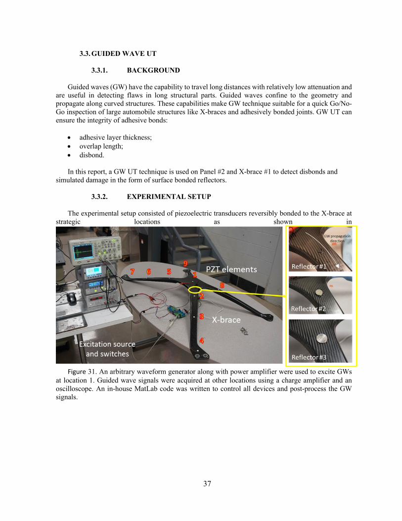
The experimental setup consisted of piezoelectric transducers reversibly bonded to the X-brace at strategic locations as shown in
Figure 31. An arbitrary waveform generator along with power amplifier were used to excite GWs
at location 1. Guided wave signals were acquired at other locations using a charge amplifier and an oscilloscope. An in-house MatLab code was written to control all devices and post-process the GW signals.
38
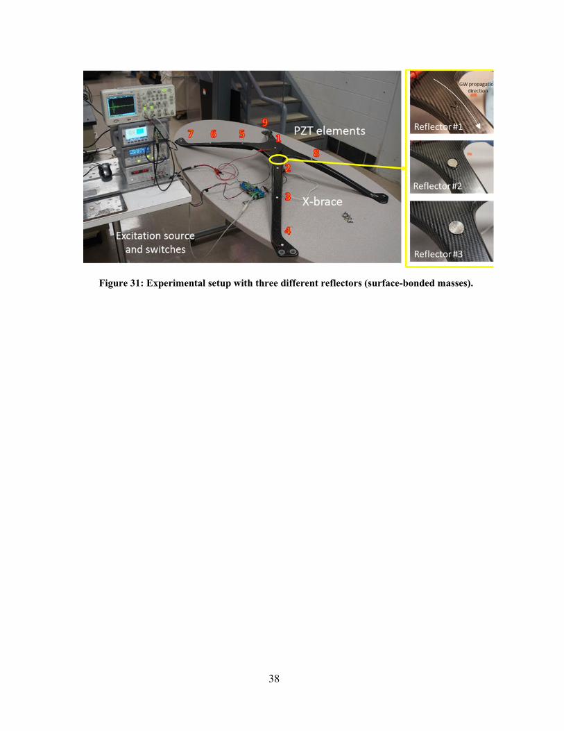
Figure 31: Experimental setup with three different reflectors (surface-bonded masses).
39
3.3.3. GUIDED WAVE UT RESULTS ON IACMI SAMPLES
This section presents experimental results of GW UT obtained in the cases of 1) detection of surface and sub-surface defects, and 2) disbonds in adhesively bonded composite / metal joints.
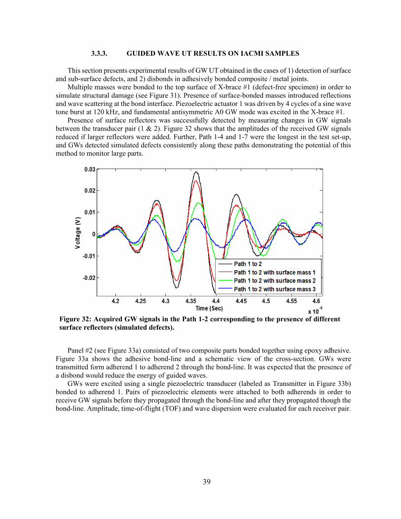
Multiple masses were bonded to the top surface of X-brace #1 (defect-free specimen) in order to simulate structural damage (see Figure 31). Presence of surface-bonded masses introduced reflections and wave scattering at the bond interface. Piezoelectric actuator 1 was driven by 4 cycles of a sine wave tone burst at 120 kHz, and fundamental antisymmetric A0 GW mode was excited in the X-brace #1.
Presence of surface reflectors was successfully detected by measuring changes in GW signals between the transducer pair (1 & 2). Figure 32 shows that the amplitudes of the received GW signals reduced if larger reflectors were added. Further, Path 1-4 and 1-7 were the longest in the test set-up, and GWs detected simulated defects consistently along these paths demonstrating the potential of this method to monitor large parts.
Figure 32: Acquired GW signals in the Path 1-2 corresponding to the presence of different surface reflectors (simulated defects).
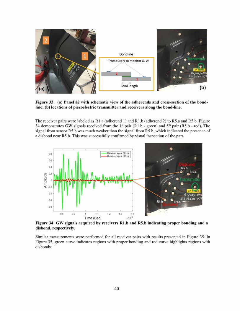
Panel #2 (see Figure 33a) consisted of two composite parts bonded together using epoxy adhesive.
Figure 33a shows the adhesive bond-line and a schematic view of the cross-section. GWs were transmitted form adherend 1 to adherend 2 through the bond-line. It was expected that the presence of a disbond would reduce the energy of guided waves.
GWs were excited using a single piezoelectric transducer (labeled as Transmitter in Figure 33b) bonded to adherend 1. Pairs of piezoelectric elements were attached to both adherends in order to receive GW signals before they propagated through the bond-line and after they propagated though the bond-line. Amplitude, time-of-flight (TOF) and wave dispersion were evaluated for each receiver pair.
40
Figure 33: (a) Panel #2 with schematic view of the adherends and cross-section of the bond-line; (b) locations of piezoelectric transmitter and receivers along the bond-line.
The receiver pairs were labeled as R1.a (adherend 1) and R1.b (adherend 2) to R5.a and R5.b. Figure 34 demonstrates GW signals received from the 1st pair (R1.b - green) and 5th pair (R5.b - red). The signal from sensor R5.b was much weaker than the signal from R5.b, which indicated the presence of a disbond near R5.b. This was successfully confirmed by visual inspection of the part.
Figure 34: GW signals acquired by receivers R1.b and R5.b indicating proper bonding and a disbond, respectively.
Similar measurements were performed for all receiver pairs with results presented in Figure 35. In Figure 35, green curve indicates regions with proper bonding and red curve highlights regions with disbonds.

41
Figure 35: Bond-line monitoring results using guided wave technique.
3.3.4. IMPACT Guided Wave UT
Results of guided wave transmission in X-brace show the ability to detect simulated surface defects and to monitor large parts. Further, results from bond-line inspection demonstrate the ability of guided wave technique to detect disbonds in adhesively bonded joints. Excitation, transmission and reception of GWs take only few milli-seconds, and thus, the overall inspection duration purely depends on the capacity of automation and signal processing unit. Advantages of Guided Wave monitoring:
• rapid GO or NO-GO inspection of large parts; • single side access; • inspection of curved surfaces.
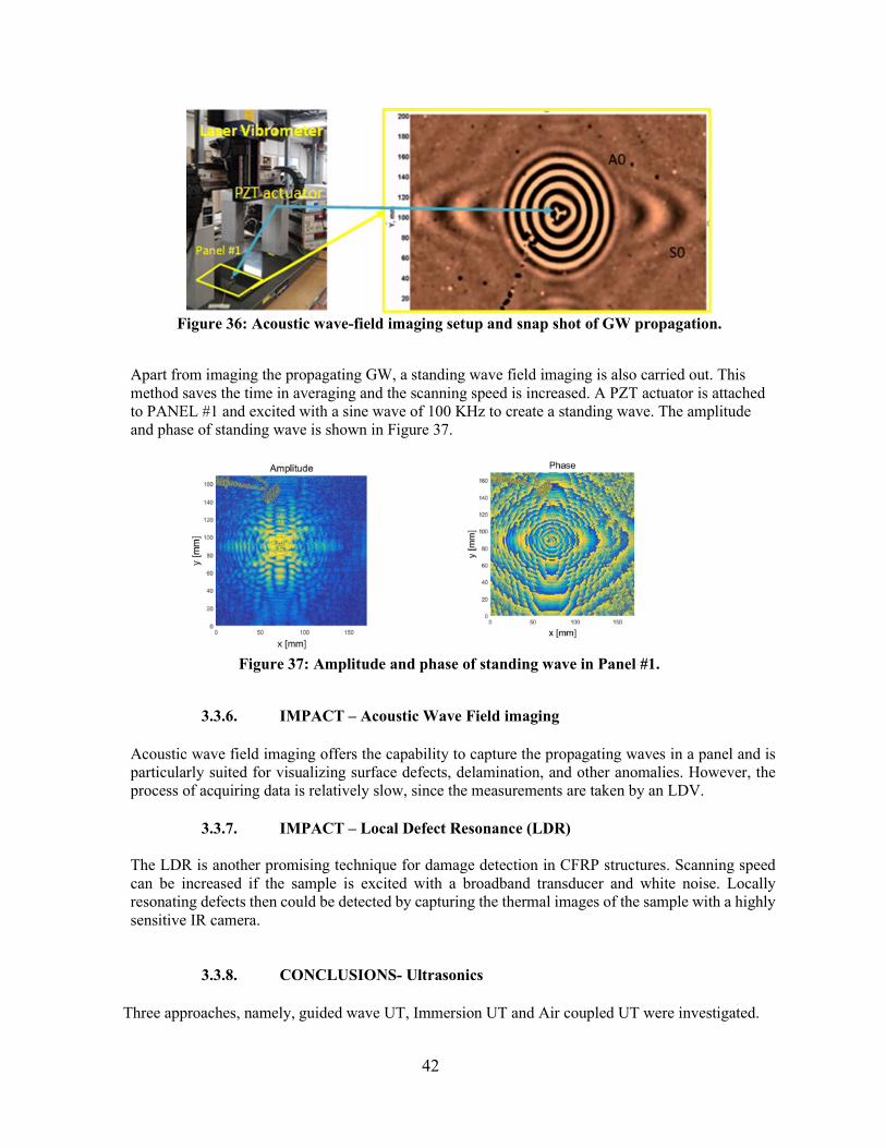
3.3.5. Acoustic Wave-field Imaging (AWI) Acoustic Wave-field Imaging (AWI) is a method to view the propagation of stress waves in structures. A Laser Doppler Vibrometer (LDV) is used to collect the out of plane displacement while the guided waves are propagating. In Figure 36, piezoelectric transducer is bonded to composite PANEL #1 through a reversible adhesive layer (Ref. Figure 36). Fundamental S0 and A0 modes are excited, and propagate radially in all directions. The group velocity of S0 mode strongly depends on direction of wave propagation owing to anisotropy of the sample. Propagating stress waves (guided waves) induce out-off plane displacements. These displacements are collected by the laser vibrometer. Data collection over the scanning area is processed to obtain a complete wave-field image as shown in Figure 36.
42
Figure 36: Acoustic wave-field imaging setup and snap shot of GW propagation.
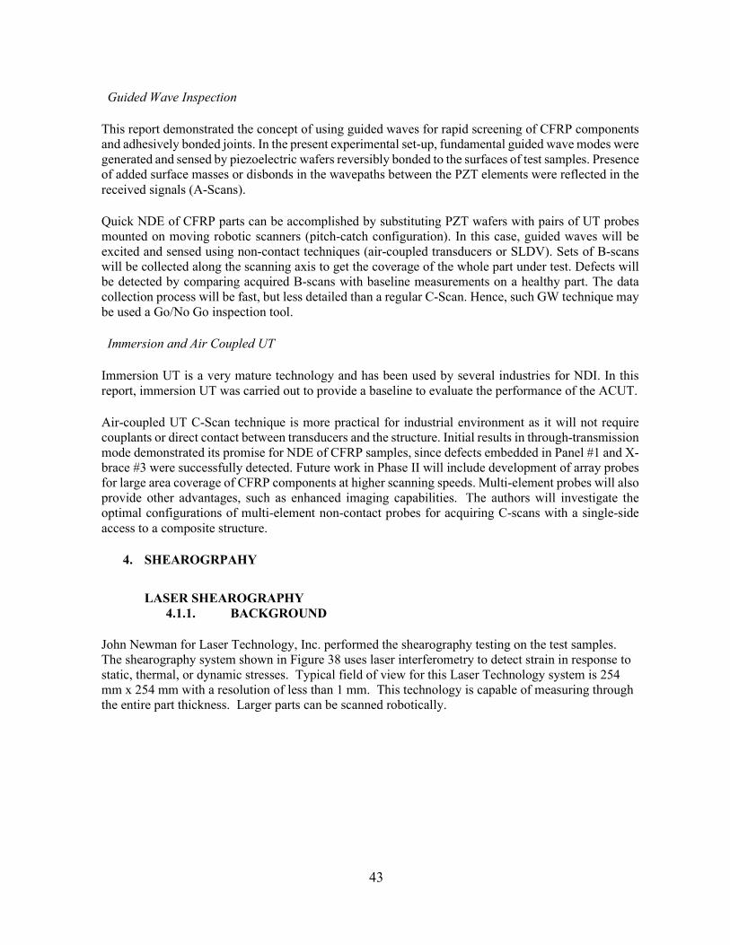
Apart from imaging the propagating GW, a standing wave field imaging is also carried out. This method saves the time in averaging and the scanning speed is increased. A PZT actuator is attached to PANEL #1 and excited with a sine wave of 100 KHz to create a standing wave. The amplitude and phase of standing wave is shown in Figure 37.
Figure 37: Amplitude and phase of standing wave in Panel #1.
3.3.6. IMPACT – Acoustic Wave Field imaging
Acoustic wave field imaging offers the capability to capture the propagating waves in a panel and is particularly suited for visualizing surface defects, delamination, and other anomalies. However, the process of acquiring data is relatively slow, since the measurements are taken by an LDV.
3.3.7. IMPACT – Local Defect Resonance (LDR)
The LDR is another promising technique for damage detection in CFRP structures. Scanning speed can be increased if the sample is excited with a broadband transducer and white noise. Locally resonating defects then could be detected by capturing the thermal images of the sample with a highly sensitive IR camera.
3.3.8. CONCLUSIONS- Ultrasonics Three approaches, namely, guided wave UT, Immersion UT and Air coupled UT were investigated.
43
Guided Wave Inspection
This report demonstrated the concept of using guided waves for rapid screening of CFRP components and adhesively bonded joints. In the present experimental set-up, fundamental guided wave modes were generated and sensed by piezoelectric wafers reversibly bonded to the surfaces of test samples. Presence of added surface masses or disbonds in the wavepaths between the PZT elements were reflected in the received signals (A-Scans).
Quick NDE of CFRP parts can be accomplished by substituting PZT wafers with pairs of UT probes mounted on moving robotic scanners (pitch-catch configuration). In this case, guided waves will be excited and sensed using non-contact techniques (air-coupled transducers or SLDV). Sets of B-scans will be collected along the scanning axis to get the coverage of the whole part under test. Defects will be detected by comparing acquired B-scans with baseline measurements on a healthy part. The data collection process will be fast, but less detailed than a regular C-Scan. Hence, such GW technique may be used a Go/No Go inspection tool.
Immersion and Air Coupled UT
Immersion UT is a very mature technology and has been used by several industries for NDI. In this report, immersion UT was carried out to provide a baseline to evaluate the performance of the ACUT.
Air-coupled UT C-Scan technique is more practical for industrial environment as it will not require couplants or direct contact between transducers and the structure. Initial results in through-transmission mode demonstrated its promise for NDE of CFRP samples, since defects embedded in Panel #1 and X-brace #3 were successfully detected. Future work in Phase II will include development of array probes for large area coverage of CFRP components at higher scanning speeds. Multi-element probes will also provide other advantages, such as enhanced imaging capabilities. The authors will investigate the optimal configurations of multi-element non-contact probes for acquiring C-scans with a single-side access to a composite structure.
4. SHEAROGRPAHY
LASER SHEAROGRAPHY 4.1.1. BACKGROUND
John Newman for Laser Technology, Inc. performed the shearography testing on the test samples. The shearography system shown in Figure 38 uses laser interferometry to detect strain in response to static, thermal, or dynamic stresses. Typical field of view for this Laser Technology system is 254 mm x 254 mm with a resolution of less than 1 mm. This technology is capable of measuring through the entire part thickness. Larger parts can be scanned robotically.

44
Figure 38: Laser Technology Inc. Shearography Measurement System
4.1.2. EXPERIMENTAL SETUP
Thermal lamps were used to heat the part in this instance. Shearography images show the part surface strain in response to the thermal input. Flaws cause a non-uniform thermal expansion of the composite material that will show up in the shearography images. Depth of defects cannot be measured with this method. Dantec Dynamics provides a similar shearography system that uses a heat source as well to excite part and can inspect an area as large as 305 mm x 305 mm. The resolution for the 305 mm x 305 mm inspection area was not specified. The Dantec Dynamics system was not available for testing.
4.1.3. SHEAROGRAPHY RESULTS ON IACMI TEST SAMPLES Thermal shearography was applied to test samples 1-5 and X-brace test sample number 1. Figure 39 shows a shearography image of the test sample no. 1 showing the known defects in the panel (as noted by the vendor). The location, angle, and dimensions of the flaws were visible.
Figure 39: Shearography image of Panel 1
45
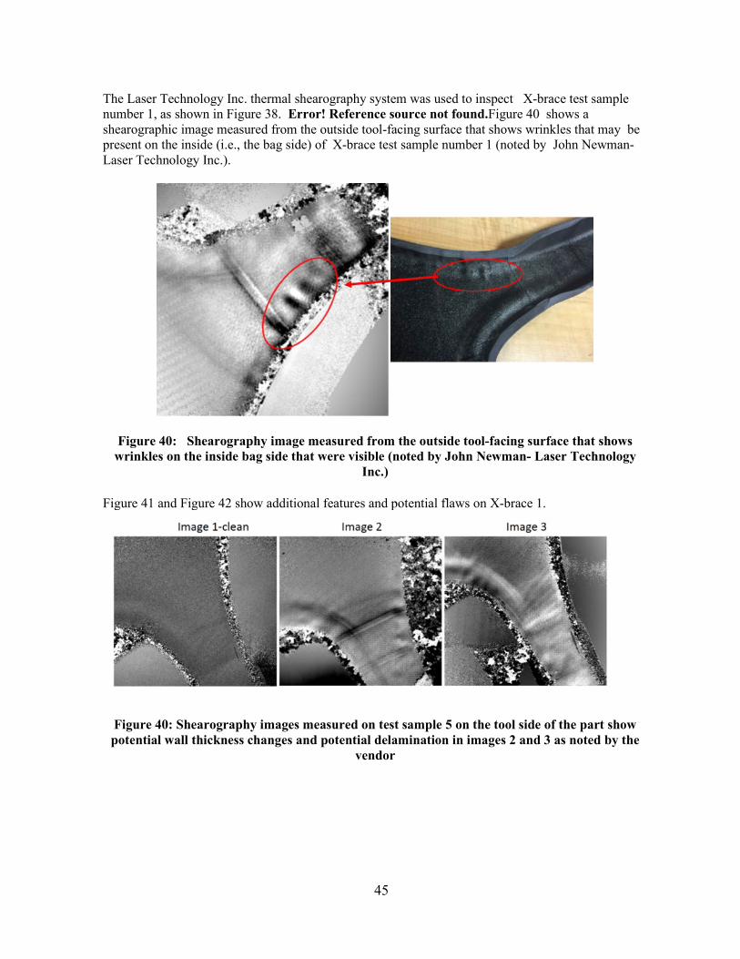
The Laser Technology Inc. thermal shearography system was used to inspect X-brace test sample number 1, as shown in Figure 38. Error! Reference source not found.Figure 40 shows a shearographic image measured from the outside tool-facing surface that shows wrinkles that may be present on the inside (i.e., the bag side) of X-brace test sample number 1 (noted by John Newman- Laser Technology Inc.).
Figure 40: Shearography image measured from the outside tool-facing surface that shows wrinkles on the inside bag side that were visible (noted by John Newman- Laser Technology
Inc.) Figure 41 and Figure 42 show additional features and potential flaws on X-brace 1.
Figure 40: Shearography images measured on test sample 5 on the tool side of the part show potential wall thickness changes and potential delamination in images 2 and 3 as noted by the
vendor

46
Figure 41: Shearography images of three arm joints of X-brace no. 1 showing potential wall thickness changes and a possible delamination in the upper right image.
This technique was also applied to Panel 2, which featured adhesively bonded thin laminates.
Figure 42 shows the results of the scan, which demonstrates the ability to inspect adhesively bonded joints for subsurface defects using this technique.

47
Figure 43 is another portion of panel 2 examining a potential adhesive disbond which can be seen from the surface.
Figure 42: Shearographic image measured on test sample no. 2. potentially showing resin rich areas (as noted by the vendor)
48
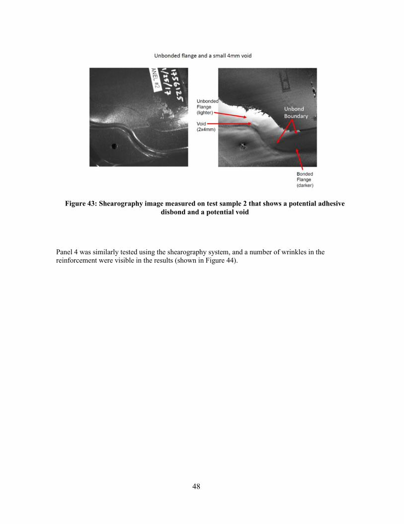
Figure 43: Shearography image measured on test sample 2 that shows a potential adhesive disbond and a potential void
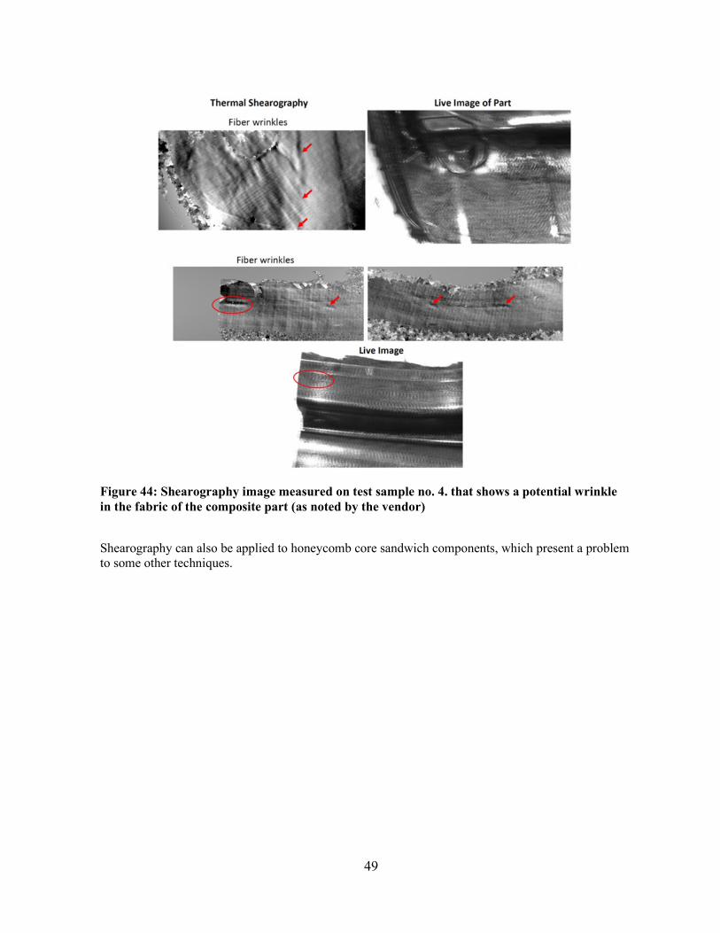
Panel 4 was similarly tested using the shearography system, and a number of wrinkles in the reinforcement were visible in the results (shown in Figure 44).
49
Figure 44: Shearography image measured on test sample no. 4. that shows a potential wrinkle in the fabric of the composite part (as noted by the vendor)
Shearography can also be applied to honeycomb core sandwich components, which present a problem to some other techniques.
50
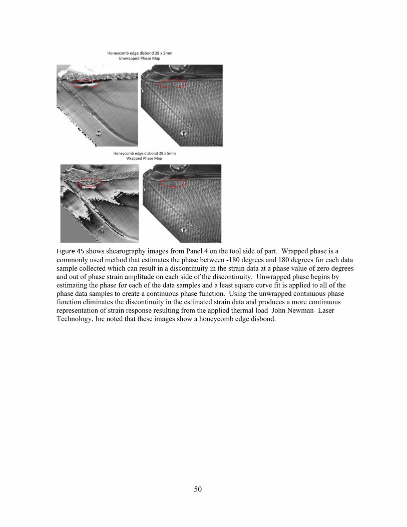
Figure 45 shows shearography images from Panel 4 on the tool side of part. Wrapped phase is a commonly used method that estimates the phase between -180 degrees and 180 degrees for each data sample collected which can result in a discontinuity in the strain data at a phase value of zero degrees and out of phase strain amplitude on each side of the discontinuity. Unwrapped phase begins by estimating the phase for each of the data samples and a least square curve fit is applied to all of the phase data samples to create a continuous phase function. Using the unwrapped continuous phase function eliminates the discontinuity in the estimated strain data and produces a more continuous representation of strain response resulting from the applied thermal load John Newman- Laser Technology, Inc noted that these images show a honeycomb edge disbond.
51
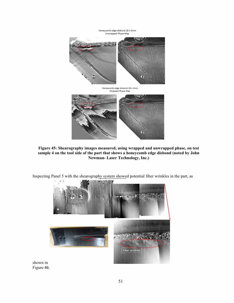
Figure 45: Shearography images measured, using wrapped and unwrapped phase, on test sample 4 on the tool side of the part that shows a honeycomb edge disbond (noted by John
Newman- Laser Technology, Inc.)
Inspecting Panel 5 with the shearography system showed potential fiber wrinkles in the part, as
shown in Figure 46.

52
Figure 46: Shearography images measured on test sample no. 5. on the bag side of part that shows a potential fiber wrinkles in the composite part (as noted by the vendor)
4.1.4 Impact- Shearography Method The shearographic inspection technique is advantageous because it produces high resolution images of defects with accurate areal location and size information. Measurement of small parts can be completed within cycle time requirements, and the sensing unit can be mounted to an industrial robot for automated inspection of larger parts. The disadvantages of this technique are that it cannot quantify the depth of defects, and the detailed high resolution results currently require expert interpretation. An estimate of shearography inspection using a Laser Technology Inc. shearography system is presented in Table 5.
Table 5: Inspection details for laser shearography system
Shearography Method
Number of pixels 1628 x 1236
Inspection duration Depends on type of automation and the part size
Coverage .45-.76 m2/minute
If expert interpretation of the results is required, time would have to be added on to the scan time to estimate the over inspection time. Data analytics could also be developed to automatically extract the location and size of potential flaws to eliminate the expert interpretation time.
53
4.1.5 Conclusions- Shearography Shearography is a wide area inspection tool that can be used for rapid inspection of composite parts. The LTI-2100 shearography sensor used for testing the test samples has a 254 mm x 254 mm field of view with a pixel resolution of 1628 x 1238 pixel , which can produce images of a part with resolution of less than 1 mm. The shearography system has integrated heat source to excite the part and well developed data processing software that is used for locating and identifying the size of flaws. Shearography is a high TRL level NDE technology that can easily be adapted to automation for rapid inspection of composite parts. However, the depth of flaws cannot be determined from the shearography results and the results do not provide information about the performance of the composite parts.
5. INFRARED IMAGING
5.1 THEMOGRAPHIC IMAGING- THERMAL WAVE IMAGING, INC
5.1.1 BACKGROUND
Thermography uses an infrared camera to measure the change in surface temperature in response to an applied heat pulse. EchoTherm - TWI™ (Thermal Wave Imaging, Inc.) flagship system is typically used for manufacturing or R&D applications. Mosaiq is the TWI software solution that allows rapid inspection of large structures, providing a subsurface image of the entire component. Thermographic Signal Reconstruction (TSR) is a TWI patented software solution that provides the ability to extract greater quantitative detail and accuracy from test samples. Precision Flash Control - an optional hardware component that allows the user to gain precise control of the timing and duration of the flash was used to "excite" the sample
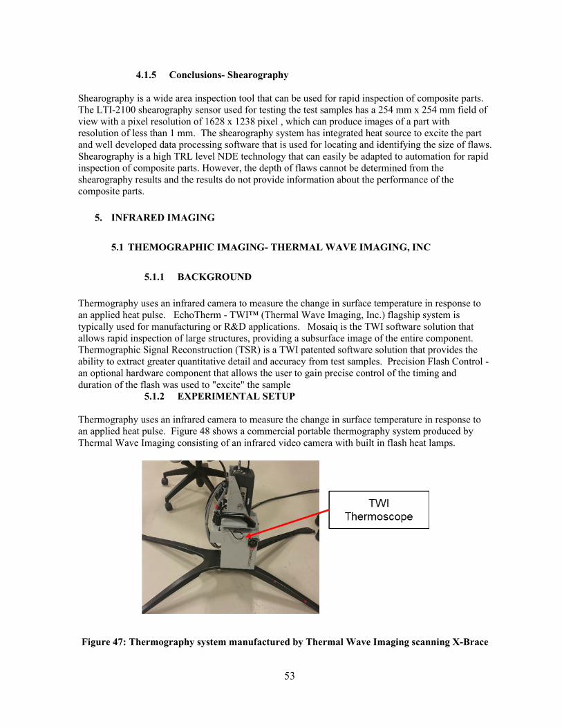
5.1.2 EXPERIMENTAL SETUP Thermography uses an infrared camera to measure the change in surface temperature in response to an applied heat pulse. Figure 48 shows a commercial portable thermography system produced by Thermal Wave Imaging consisting of an infrared video camera with built in flash heat lamps.
Figure 47: Thermography system manufactured by Thermal Wave Imaging scanning X-Brace

54
This example thermographic imaging system has a field of view of 305 mm x 229 mm with a resolution of 0.5 mm. The depth of the flaws that can be measured is dependent on material and flaw, but flaws near the surface are more easily measured. This system can detect a 1/8” cross-drilled hole at 1mm depth and a ¼” hole at 3mm depth in carbon-carbon composite. In operation, the built-in flash lamps apply a burst of heat to the part. The infrared camera records thermal images of the part as it is heated and cooled. Defects will transfer heat at a different rate than the surrounding composite material and will show up as changes in temperature in the IR images. The portable Thermal Wave Imaging Inc. (TWI) flash thermography unit shown in Figure 47 was used by Steve Shepard- Themal Wave imaging to inspect the IACMI test samples 2-5. This unit contained both a flash heat excitation source and an infrared camera to record thermal video. The thermal video was processed using Thermographic Signal Reconstruction in TWI’s proprietary software.
5.1.3 THERMOGRAPHIC IMAGING RESULTS ON IACMI TEST SAMPLES
IACMI Panel 2 provides an opportunity to inspect adhesively bonded thin laminates. Thermal images were acquired on Panel 2, and separate images were stitched together using the TWIsoftware. Figure 48 shows the results of the scan, showing several anomalies on the bond line, and demonstrating the ability to inspect both the laminates and the adhesive bonds.
Figure 48: Thermal image measured on Panel 2 showing several anomalies at locations labeled a-e (TWI did not identify the type of defects at locations a-e)
Figure 50 shows a thermographic image of test sample no. 3. The vendor did not note any potential

55
flaws in the part
Figure 49: Thermographic image of test sample 3 - no defects were noted by the vendor
Figure 50 shows a thermographic image of test sample no. 4. Potential delaminations were identified (noted by the vendor) around the machined holes. Figure 51 shows a thermographic image of test sample no. 5 and no potential flaws were identified by the vendor.

56
Figure 50: Thermographic images of test sample 4 - potential delaminations were noted by the vendor around machined holes
Figure 51: Thermographic image of test sample 5 - no flaws were noted by the vendor
5.1.4 Impact- Infrared thermography method
The advantages of thermographic imaging are that it produces high resolution images of defects, can
57
detect and locate flaws in thin composite parts including sensing the depth of flaws in thin composite parts. Small parts can be scanned in a single image, while larger parts can be scanned using an industrial robot. The disadvantages of this technique are that the cycle time is long for thick composite parts, and there is a limit on the thickness of part, which could be measured. Like the shearography system, the results are an image of the part, which require expert interpretation. An estimate of infrared imaging inspection using a Thermal Wave Imaging Inc. (TWI) system is presented in Table 6.
Table 6: Inspection details for infrared thermographic imaging system
Thermography Method
Inspection duration Depends on type of automation and the part size
Coverage .07-.14 m2/minute
5.1.5 Conclusions- Thermography Infrared imaging is a wide area inspection tool that can be used for rapid inspection of composite parts. The TWI thermoscope sensor used for testing the test samples has a 304 mm x 228 mm field of view that can produce images of a part with resolution of less than 1 mm. The TWI system has a built-in heat source to excite the part and comes with well-developed data processing software that is used to locate and identify the size and depth of flaws in the CFRP parts. Inspecting thick section of a part can take additional time and will increase the cycle time of the overall inspection. Thermography is a high TRL level NDE technology that can easily be adapted to automation for rapid inspection of composite parts. However, the infrared imaging results do not provide information about the performance of the composite parts.
6. MICROWAVE METHOD
6.1 DIELCETRIC TESTING- MWI LABS, INC
6.1.1. BACKGROUND Material-Wave Interactions (MWI) labs produces a hand held linear-polarized microwave sensor. The MWI system consists of a resonator designed for a particular application along with a commercial, off-the-shelf, vector network analyzer (VNA). The part can be scanned manually with the Epod sensor point by point to determine the uniformity of the Gaussian resonate peak magnitude. The Gaussian resonate peak is monitored with a VNA. Changes in the magnitude of the Gaussian resonant peak can indicate the presence of defects. The resonant spot size in this particular application was 1.25”. Larger parts could be scanned robotically.
6.1.2. EXPERIMENTAL SETUP
Figure 53 shows the MWI Labs system with the resonator and the vector network analyzer (VNA). The part was scanned manually with the Epod sensor point by point to determine the uniformity of
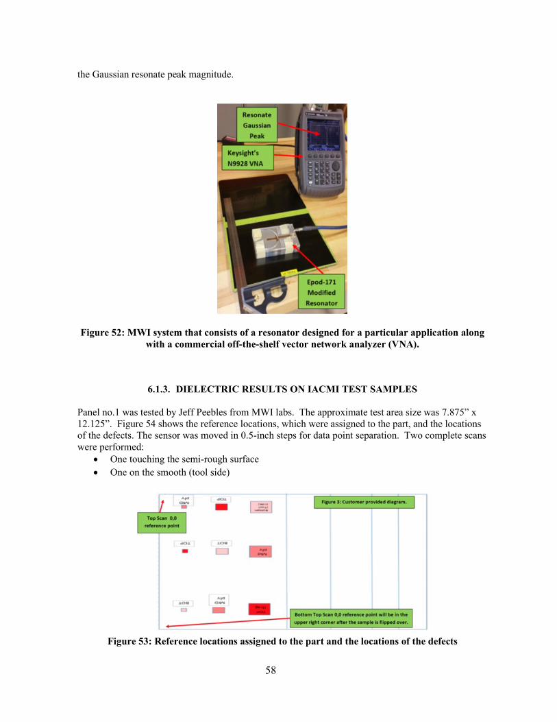
58
the Gaussian resonate peak magnitude.
Figure 52: MWI system that consists of a resonator designed for a particular application along with a commercial off-the-shelf vector network analyzer (VNA).
6.1.3. DIELECTRIC RESULTS ON IACMI TEST SAMPLES Panel no.1 was tested by Jeff Peebles from MWI labs. The approximate test area size was 7.875” x 12.125”. Figure 54 shows the reference locations, which were assigned to the part, and the locations of the defects. The sensor was moved in 0.5-inch steps for data point separation. Two complete scans were performed:
• One touching the semi-rough surface • One on the smooth (tool side)
Figure 53: Reference locations assigned to the part and the locations of the defects
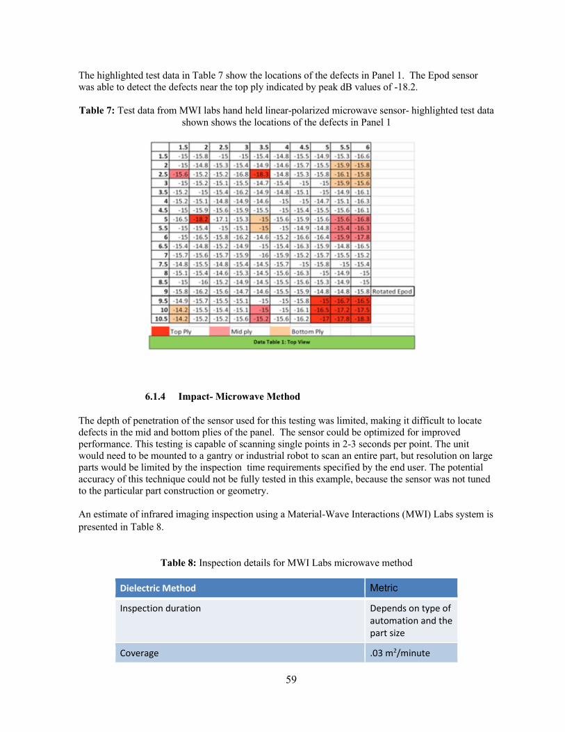
59
The highlighted test data in Table 7 show the locations of the defects in Panel 1. The Epod sensor was able to detect the defects near the top ply indicated by peak dB values of -18.2. Table 7: Test data from MWI labs hand held linear-polarized microwave sensor- highlighted test data
shown shows the locations of the defects in Panel 1
6.1.4 Impact- Microwave Method
The depth of penetration of the sensor used for this testing was limited, making it difficult to locate defects in the mid and bottom plies of the panel. The sensor could be optimized for improved performance. This testing is capable of scanning single points in 2-3 seconds per point. The unit would need to be mounted to a gantry or industrial robot to scan an entire part, but resolution on large parts would be limited by the inspection time requirements specified by the end user. The potential accuracy of this technique could not be fully tested in this example, because the sensor was not tuned to the particular part construction or geometry. An estimate of infrared imaging inspection using a Material-Wave Interactions (MWI) Labs system is presented in Table 8.
Table 8: Inspection details for MWI Labs microwave method
Dielectric Method Metric
Inspection duration Depends on type of automation and the part size
Coverage .03 m2/minute
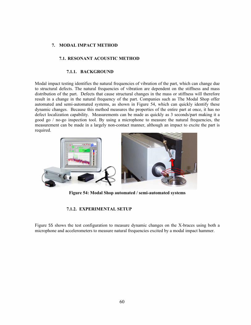
60
7. MODAL IMPACT METHOD
7.1. RESONANT ACOUSTIC METHOD
7.1.1. BACKGROUND
Modal impact testing identifies the natural frequencies of vibration of the part, which can change due to structural defects. The natural frequencies of vibration are dependent on the stiffness and mass distribution of the part. Defects that cause structural changes in the mass or stiffness will therefore result in a change in the natural frequency of the part. Companies such as The Modal Shop offer automated and semi-automated systems, as shown in Figure 54, which can quickly identify these dynamic changes. Because this method measures the properties of the entire part at once, it has no defect localization capability. Measurements can be made as quickly as 3 seconds/part making it a good go / no-go inspection tool. By using a microphone to measure the natural frequencies, the measurement can be made in a largely non-contact manner, although an impact to excite the part is required.
Figure 54: Modal Shop automated / semi-automated systems
7.1.2. EXPERIMENTAL SETUP
Figure 55 shows the test configuration to measure dynamic changes on the X-braces using both a microphone and accelerometers to measure natural frequencies excited by a modal impact hammer.
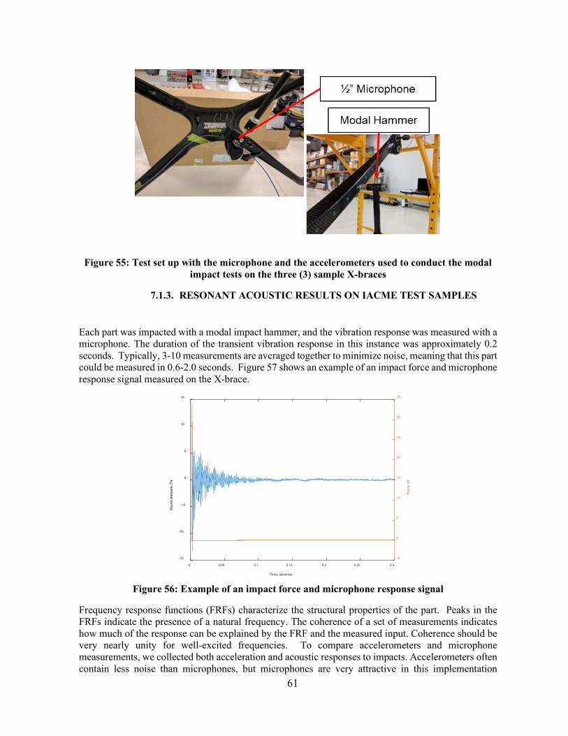
61
Figure 55: Test set up with the microphone and the accelerometers used to conduct the modal impact tests on the three (3) sample X-braces
7.1.3. RESONANT ACOUSTIC RESULTS ON IACME TEST SAMPLES Each part was impacted with a modal impact hammer, and the vibration response was measured with a microphone. The duration of the transient vibration response in this instance was approximately 0.2 seconds. Typically, 3-10 measurements are averaged together to minimize noise, meaning that this part could be measured in 0.6-2.0 seconds. Figure 57 shows an example of an impact force and microphone response signal measured on the X-brace.
Figure 56: Example of an impact force and microphone response signal
Frequency response functions (FRFs) characterize the structural properties of the part. Peaks in the FRFs indicate the presence of a natural frequency. The coherence of a set of measurements indicates how much of the response can be explained by the FRF and the measured input. Coherence should be very nearly unity for well-excited frequencies. To compare accelerometers and microphone measurements, we collected both acceleration and acoustic responses to impacts. Accelerometers often contain less noise than microphones, but microphones are very attractive in this implementation
0 0.05 0.1 0.15 0.2 0.25 0.3
Time, seconds
-15
-10
-5
0
5
10
15
Soun
d pr
essu
re, P
a
-5
0
5
10
15
20
25
30
35
Forc
e, lb
f

62
because they do not require contact with the part. Figure 58 shows that the accelerometer measurement has a more consistent coherence below 500 Hz, but both measurements clearly show resonant frequencies between 400-5000 Hz, so the more convenient non-contact microphone measurement would be sufficient in this application.
Figure 57: Comparison of microphone and accelerometer FRFs on X-brace test sample
The test on the three X-braces showed significant differences in the natural frequencies between parts. Differences in natural frequencies are shown in the FRF comparison in Figure 58.
Figure 58: FRF’s measured with a ½” microphone on the three (3) X-braces
This shift in natural frequencies indicates an anomaly in either the stiffness or the mass distributions of
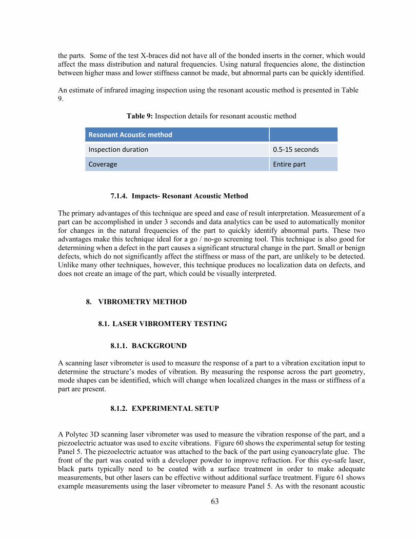
63
the parts. Some of the test X-braces did not have all of the bonded inserts in the corner, which would affect the mass distribution and natural frequencies. Using natural frequencies alone, the distinction between higher mass and lower stiffness cannot be made, but abnormal parts can be quickly identified. An estimate of infrared imaging inspection using the resonant acoustic method is presented in Table 9.
Table 9: Inspection details for resonant acoustic method
Resonant Acoustic method
Inspection duration 0.5-15 seconds
Coverage Entire part
7.1.4. Impacts- Resonant Acoustic Method The primary advantages of this technique are speed and ease of result interpretation. Measurement of a part can be accomplished in under 3 seconds and data analytics can be used to automatically monitor for changes in the natural frequencies of the part to quickly identify abnormal parts. These two advantages make this technique ideal for a go / no-go screening tool. This technique is also good for determining when a defect in the part causes a significant structural change in the part. Small or benign defects, which do not significantly affect the stiffness or mass of the part, are unlikely to be detected. Unlike many other techniques, however, this technique produces no localization data on defects, and does not create an image of the part, which could be visually interpreted.
8. VIBROMETRY METHOD
8.1. LASER VIBROMTERY TESTING
8.1.1. BACKGROUND A scanning laser vibrometer is used to measure the response of a part to a vibration excitation input to determine the structure’s modes of vibration. By measuring the response across the part geometry, mode shapes can be identified, which will change when localized changes in the mass or stiffness of a part are present.
8.1.2. EXPERIMENTAL SETUP A Polytec 3D scanning laser vibrometer was used to measure the vibration response of the part, and a piezoelectric actuator was used to excite vibrations. Figure 60 shows the experimental setup for testing Panel 5. The piezoelectric actuator was attached to the back of the part using cyanoacrylate glue. The front of the part was coated with a developer powder to improve refraction. For this eye-safe laser, black parts typically need to be coated with a surface treatment in order to make adequate measurements, but other lasers can be effective without additional surface treatment. Figure 61 shows example measurements using the laser vibrometer to measure Panel 5. As with the resonant acoustic

64
method, natural frequencies of vibration can be quantified using this technique, but in addition, this approach gives the ability to calculate the spatial deflection of a vibration mode, called the mode shape. Compared to natural frequencies alone, mode shapes can be more sensitive to localized changes in the structure. Figure 62 shows two operating deflection shapes measured on Panel 5 using the laser vibrometer, which are closely related to the fundamental bending mode shape at higher frequencies. Changes in the localized bending in these higher frequency mode shapes caused by presence of defects can be identified use modal curvature [4]. [4] Adams, D. and Meyer, J., “Detecting Changes in Fiber Orientation in a Simulated Chopped Fiber Plate Using Curvature Mode Shapes” ASME Journal of Applied Mechanics, MAY 2018, Vol. 85 / 051009-1, DOI: 10.1115/1.4039479
Figure 59: Scanning laser vibrometer setup showing test configuration for Panel 5
Figure 60: Frequency response functions for Panel 5 using scanning laser vibrometer
200 400 600 800 1000 1200 1400 1600 1800 2000
Frequency, Hz
10-7
10-6
10-5
10-4
10-3
10-2
|FR
F| -
mm
/s/N
X
Y
Z
Actuator
Panel 5
3D Laser Vibrometer

65
Figure 61: Two operating deflection shapes measured on Panel 5 using the laser vibrometer, which are closely related to the fundamental bending mode shape at higher frequencies Impacts- Laser Vibrometry
The advantage of laser vibrometry is the capability of measuring three dimensional deflections in a part without attaching a large number of sensors to the part. The downside to this capability is the increased cycle time compared to other vibration measurement techniques such as impact tests. The part must be excited with a continuous vibration input, which is of longer duration than an impact. Cycle times of 10 seconds per point measurement are common, meaning that a high-resolution scan of the part would not fit into the cycle time requirements without compromising on the quality of measurement. An estimate of infrared imaging inspection using 3D laser vibrometry is presented in Table 10.
Table 10: Inspection details for 3D laser vibrometry
Vibrometry method
Inspection duration 10s/point, approximately 5-15 minutes total
Coverage Wide area
9. PROFILOMETRY METHOD
9.1. LASER PROFILOMETRY
9.1.1. BACKGROUND Laser Profilometry is a technology used to quickly and precisely measure the outer profile of a part, as shown in Figure 63. In this application, the non-contact profile measurement could be used to detect geometrical flaws on the surface of the part. This profile measurement could be used to ensure that the manufactured part geometry is within specified tolerances, and could potentially detect flaws such as missing plies or incorrect preform layup if the problem manifested itself at the surface of the part.

66
Figure 62: Laser profilometers manufactured by Keyence
9.1.2. EXPERIMENTAL SETUP
This laser profilometry system has a vertical resolution of 1μm, and a resolution of 100μm along the width of the laser beams. For this test, the part was moved under the profilometer at fixed speed as the surface displacement of the part was recorded with a data acquisition system to map the surface of the part. Figure 63 shows the test setup for measuring Panel 1 with the laser profilometer.
Figure 63: Test setup for measuring Panel 1 with the laser profilometer
9.1.3. LASER PROFILOMETRY RESULTS ON IACMI TEST SAMPLES The results from this test, shown in Figure 65, indicate that this laser profilometer is capable of measuring the surface geometry of a carbon fiber part at high resolution and speed without any surface treatment or preparation.
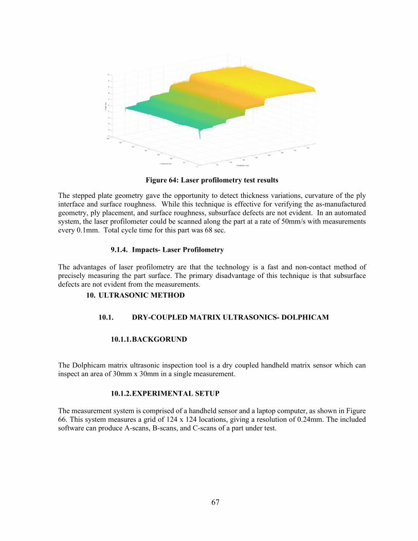
67
Figure 64: Laser profilometry test results
The stepped plate geometry gave the opportunity to detect thickness variations, curvature of the ply interface and surface roughness. While this technique is effective for verifying the as-manufactured geometry, ply placement, and surface roughness, subsurface defects are not evident. In an automated system, the laser profilometer could be scanned along the part at a rate of 50mm/s with measurements every 0.1mm. Total cycle time for this part was 68 sec.
9.1.4. Impacts- Laser Profilometry The advantages of laser profilometry are that the technology is a fast and non-contact method of precisely measuring the part surface. The primary disadvantage of this technique is that subsurface defects are not evident from the measurements.
10. ULTRASONIC METHOD
10.1. DRY-COUPLED MATRIX ULTRASONICS- DOLPHICAM
10.1.1. BACKGORUND The Dolphicam matrix ultrasonic inspection tool is a dry coupled handheld matrix sensor which can inspect an area of 30mm x 30mm in a single measurement.
10.1.2. EXPERIMENTAL SETUP The measurement system is comprised of a handheld sensor and a laptop computer, as shown in Figure 66. This system measures a grid of 124 x 124 locations, giving a resolution of 0.24mm. The included software can produce A-scans, B-scans, and C-scans of a part under test.
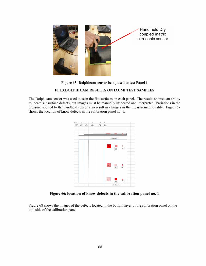
68
Figure 65: Dolphicam sensor being used to test Panel 1
10.1.3. DOLPHICAM RESULTS ON IACMI TEST SAMPLES The Dolphicam sensor was used to scan the flat surfaces on each panel. The results showed an ability to locate subsurface defects, but images must be manually inspected and interpreted. Variations in the pressure applied to the handheld sensor also result in changes in the measurement quality. Figure 67 shows the location of know defects in the calibration panel no. 1.
Figure 66: location of know defects in the calibration panel no. 1
Figure 68 shows the images of the defects located in the bottom layer of the calibration panel on the tool side of the calibration panel.
Hand held Dry coupled matrix
ultrasonic sensor
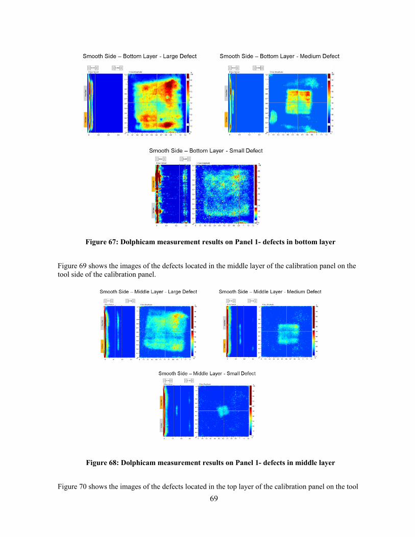
69
Figure 67: Dolphicam measurement results on Panel 1- defects in bottom layer
Figure 69 shows the images of the defects located in the middle layer of the calibration panel on the tool side of the calibration panel.
Figure 68: Dolphicam measurement results on Panel 1- defects in middle layer
Figure 70 shows the images of the defects located in the top layer of the calibration panel on the tool
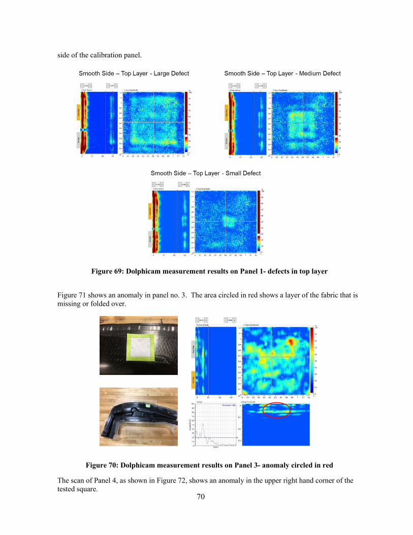
70
side of the calibration panel.
Figure 69: Dolphicam measurement results on Panel 1- defects in top layer
Figure 71 shows an anomaly in panel no. 3. The area circled in red shows a layer of the fabric that is missing or folded over.
Figure 70: Dolphicam measurement results on Panel 3- anomaly circled in red
The scan of Panel 4, as shown in Figure 72, shows an anomaly in the upper right hand corner of the tested square.
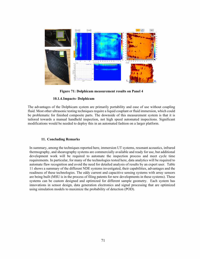
71
Figure 71: Dolphicam measurement results on Panel 4
10.1.4. Impacts- Dolphicam The advantages of the Dolphicam system are primarily portability and ease of use without coupling fluid. Most other ultrasonic testing techniques require a liquid couplant or fluid immersion, which could be problematic for finished composite parts. The downside of this measurement system is that it is tailored towards a manual handheld inspection, not high speed automated inspections. Significant modifications would be needed to deploy this in an automated fashion on a larger platform.
11. Concluding Remarks In summary, among the techniques reported here, immersion UT systems, resonant acoustics, infrared thermography, and shearography systems are commercially available and ready for use, but additional development work will be required to automate the inspection process and meet cycle time requirements. In particular, for many of the technologies tested here, data analytics will be required to automate flaw recognition and avoid the need for detailed analysis of results by an expert user. Table 11 shows a summary of the different NDE systems investigated, their capabilities, advantages and the readiness of these technologies. The eddy current and capacitive sensing systems with array sensors are being built (MSU is in the process of filing patents for new developments in these systems). These systems can be custom designed and optimized for different sample geometry. Each system has innovations in sensor design, data generation electronics and signal processing that are optimized using simulation models to maximize the probability of detection (POD).

72
Table 11: Summary of NDE technologies investigated
The following metrics were used to evaluate each NDE technology as potential end of line inspection tools:
• detection accuracy • inspection speed • coverage area, • industrial durability • group or classify the composite parts based on geometry and performance requirements of
the composite part. The non-academic/non-supplier team members eliminated the following NDE technologies from consideration prior to rating process:
• Resonant Acoustic – not selected due to flaw size and believed to be insensitive to low levels
NDE Technology
Type of output Features of technique Types of defects TRL
Non-contact Fiber BreakageSingle-side access Fiber WavinessExpendable to array sensor Foreign Object DebrisDepth of inspection – up to 0.5” Thickness VariationsResolution depends on sensor size Improper Curing
Resin-rich AreasNon-contact Interlaminar DelaminationSingle-side access Fiber BreakageExpendable to array sensor Foreign Object DebrisDepth of inspection – up to 0.25” Thickness VariationsResolution depends on sensor size Improper Curing
Resin-rich AreasTransducers mounted into water jet nozzles Interlaminar DelaminationSingle-side access Fiber BreakageExpandable to phased array sensors Foreign Object DebrisDepth of inspection - ~inches Thickness VariationsHigh resolution Improper Curing
Resin-rich AreasInterface DisbondsPorosity/Agglomerations of Air Voids
No couplants Interlaminar DelaminationSingle-side access Fiber BreakageExpandable to array sensors Foreign Object DebrisDepth of inspection – 0.35” Thickness VariationsMedium resolution Improper Curing
Resin-rich AreasInterface DisbondsPorosity/Agglomerations of Air Voids
Contact and non-contact modes Interlaminar DelaminationSingle-side access Fiber BreakageLarge area coverage/ Fast scans Foreign Object DebrisSuited for curved surfaces Interface DisbondsMedium resolutionAdvanced signal processing is needed
9(Commercially available)
9(Commercially available)
MWI RF DielectricRF resonant frequency / amplitude
Non-contact or dry contact Thickness variations, FOD, improper cure, resin rich areas
7
9(Commercially available)
Laser vibrometryVibration mode shape and natural frequency
High resolution 3D dynamics measurement, flaws linked to dynamic properties
Ply layup errors, delaminations / disbonds, broken fibers, thickness variations, resin-rich/lean areas, incomplete cure
7
9(Commercially available)
9 (Commercially available)
Laser profilometry Outer surface profileNon-contact, no surface preparation, direct geometry measurement,
Thickness variations, geometrical defects,
Dolphicam A, B, C ScansDry coupled handheld sensor, matrix measurement, single-sided access
Delamination, broken fibers, thickness variations, interface disbonds, foreign object debris
Thermography Surface temperatureNon-contact, single-sided access, high resolution, visual presentation of results
Delaminations / disbonds, bond line variation, FOD, broken fibers, thickness
Modal impact testing
Natural frequencies of vibration
Very short cycle time, detects flaws which alter the structural integrity, non-contact
Ply layup errors, delaminations / disbonds, broken fibers, thickness variations, resin-
Guided wave B-scan Not commercially available
Shearography Surface strain fieldNon-contact, single-sided access, through part inspection, high resolution, visual presentation of
Delaminations / disbonds, bond line variation, FOD, broken fibers, thickness
Water-Coupled UT C-Scan (3D Image) Commercially available
Air-Coupled UT C-scan (3D Image)Single sensor systems are
commercially available
Eddy Current C-scan (Coil Impedance)
Commercially available for inspection of metals. Systems
adapted to inspection of CFRP are not commercially available.
Capacitive Sensing C-scan (Voltage)Systems are not commercially
available
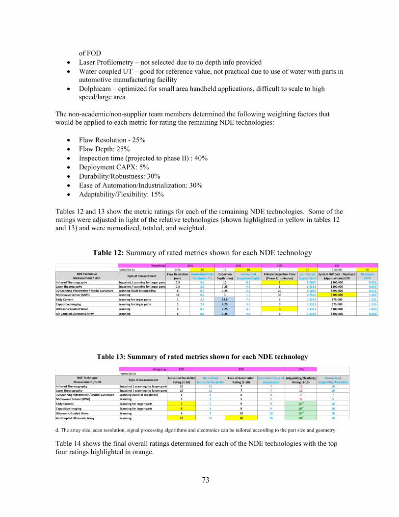
73
of FOD • Laser Profilometry – not selected due to no depth info provided • Water coupled UT – good for reference value, not practical due to use of water with parts in
automotive manufacturing facility • Dolphicam – optimized for small area handheld applications, difficult to scale to high
speed/large area The non-academic/non-supplier team members determined the following weighting factors that would be applied to each metric for rating the remaining NDE technologies:
• Flaw Resolution - 25% • Flaw Depth: 25% • Inspection time (projected to phase II) : 40% • Deployment CAPX: 5% • Durability/Robustness: 30% • Ease of Automation/Industrialization: 30% • Adaptability/Flexibility: 15%
Tables 12 and 13 show the metric ratings for each of the remaining NDE technologies. Some of the ratings were adjusted in light of the relative technologies (shown highlighted in yellow in tables 12 and 13) and were normalized, totaled, and weighted.
Table 12: Summary of rated metrics shown for each NDE technology
Table 13: Summary of rated metrics shown for each NDE technology
d. The array size, scan resolution, signal processing algorithms and electronics can be tailored according to the part size and geometry. Table 14 shows the final overall ratings determined for each of the NDE technologies with the top four ratings highlighted in orange.
Weighting: 40% 5%normalize to 0.24 10 16 10 1 10 $10,000 10
Infrared Thermography Snapshot / scanning for larger parts 0.3 8.0 10 6.3 1 5.0000 $200,000 0.500 Laser Shearography Snapshot / scanning for larger parts 0.3 8.0 7.25 4.5 3 3.3333 $200,000 0.500 3D Scanning Vibrometer / Modal Curvature Scanning (Built-in capability) 6 0.4 7.25 4.5 20 0.5000 $890,000 0.112 Microwave Sensor (MWI) Scanning 10 0.2 3 1.9 39 0.2564 $100,000 1.000 Eddy Current Scanning for larger parts 1 2.4 12.5 7.8 3 3.3333 $75,000 1.333 Capacitive Imaging Scanning for larger parts 1 2.4 6.25 3.9 3 3.3333 $75,000 1.333 Ultrasonic Guided Wave Scanning 5 0.5 7.25 4.5 3 3.3333 $100,000 1.000 Air-Coupled Ultrasonic Array Scanning 5 0.5 7.25 4.5 3 3.3333 $200,000 0.500
Deployed
CAPX
25% 25%
NDE Technique Measurement / Unit
Type of measurement Flaw Resolution (mm)
Normalized Flaw Resolution ^-1
Inspection Depth (mm)
Normalized Inspection Depth
X-Brace Inspection Time (Phase 2) (minutes)
normalized Inspect Time
System HW Cost - Deployed (Approximate) USD
Weighting: 30% 30% 15%normalize to
Adapability/FlexibilityRating (1-10)
Infrared Thermography Snapshot / scanning for larger parts 10 10 7 7 10 10Laser Shearography Snapshot / scanning for larger parts 10 10 7 7 10 103D Scanning Vibrometer / Modal Curvature Scanning (Built-in capability) 4 4 6 6 7 7Microwave Sensor (MWI) Scanning 5 5 5 5 5 5Eddy Current Scanning for larger parts 7 7 9 9 10 d 10Capacitive Imaging Scanning for larger parts 6 6 9 9 10 d 10Ultrasonic Guided Wave Scanning 9 9 10 10 10 d 10Air-Coupled Ultrasonic Array Scanning 10 10 10 10 10 d 10
Normalized Adapability/Flexibility
Industrial Durability Rating (1-10)
Normalized Industrial Durability
Ease of Automation Rating (1-10)
Normalized Ease of Automation
NDE Technique Measurement / Unit
Type of measurement
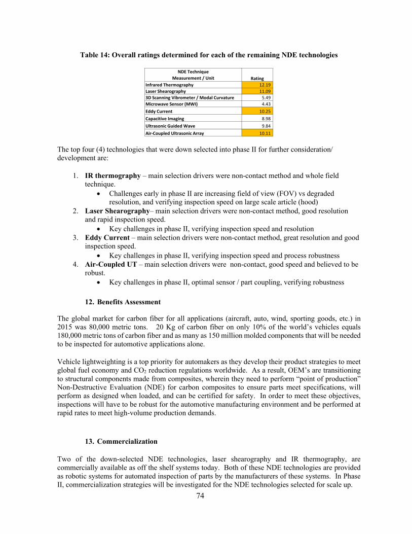
74
Table 14: Overall ratings determined for each of the remaining NDE technologies
The top four (4) technologies that were down selected into phase II for further consideration/ development are:
1. IR thermography – main selection drivers were non-contact method and whole field technique.
• Challenges early in phase II are increasing field of view (FOV) vs degraded resolution, and verifying inspection speed on large scale article (hood)
2. Laser Shearography– main selection drivers were non-contact method, good resolution and rapid inspection speed.
• Key challenges in phase II, verifying inspection speed and resolution 3. Eddy Current – main selection drivers were non-contact method, great resolution and good
inspection speed. • Key challenges in phase II, verifying inspection speed and process robustness
4. Air-Coupled UT – main selection drivers were non-contact, good speed and believed to be robust.
• Key challenges in phase II, optimal sensor / part coupling, verifying robustness
12. Benefits Assessment The global market for carbon fiber for all applications (aircraft, auto, wind, sporting goods, etc.) in 2015 was 80,000 metric tons. 20 Kg of carbon fiber on only 10% of the world’s vehicles equals 180,000 metric tons of carbon fiber and as many as 150 million molded components that will be needed to be inspected for automotive applications alone. Vehicle lightweighting is a top priority for automakers as they develop their product strategies to meet global fuel economy and CO2 reduction regulations worldwide. As a result, OEM’s are transitioning to structural components made from composites, wherein they need to perform “point of production” Non-Destructive Evaluation (NDE) for carbon composites to ensure parts meet specifications, will perform as designed when loaded, and can be certified for safety. In order to meet these objectives, inspections will have to be robust for the automotive manufacturing environment and be performed at rapid rates to meet high-volume production demands.
13. Commercialization Two of the down-selected NDE technologies, laser shearography and IR thermography, are commercially available as off the shelf systems today. Both of these NDE technologies are provided as robotic systems for automated inspection of parts by the manufacturers of these systems. In Phase II, commercialization strategies will be investigated for the NDE technologies selected for scale up.
Infrared Thermography 12.19 Laser Shearography 11.09 3D Scanning Vibrometer / Modal Curvature 5.49 Microwave Sensor (MWI) 4.43 Eddy Current 10.25 Capacitive Imaging 8.98 Ultrasonic Guided Wave 9.84 Air-Coupled Ultrasonic Array 10.11
RatingNDE Technique
Measurement / Unit

75
LEAD PARTNER BACKGROUND American Chemistry Council (ACC) Plastics Division ACC is committed to sustainable development by fostering progress in our economy, environment and society. ACC’s 160 member companies are engaged in the business of chemistry, an innovative $768 billion enterprise that is helping solve the biggest challenges facing our nation and the world. The business of chemistry, which includes manufacturing of lightweight polymer composites used by the transportation industry, creates over 811,000 U.S. manufacturing and high-tech jobs, plus six million related jobs that support families and communities. Our members are committed to providing innovative, economical solutions to lightweight vehicles while preserving and improving safety and design flexibility while enabling emerging technologies, including autonomous and electric vehicles.