Development of Novel Eddy Current

Dampers for the Suppression of

Structural Vibrations

by

Henry A. Sodano

Dissertation Submitted to the Faculty of the

Virginia Polytechnic Institute and State University

in partial fulfillment of the requirements for the degree of

Doctorate of Philosophy in

Mechanical Engineering

Dr. Daniel J. Inman, Chair Dr. Donald J. Leo Dr. Gyuhae Park

Dr. Harry H. Robertshaw Dr. W. Keith Belvin

May 5, 2005 Blacksburg, Virginia

Keywords: Eddy current damper, inflatable satellite, electromagnetic damper, membrane,

vibration suppression, viscous damping, magnetic damping

Copyright 2005, Henry A. Sodano

Development of Novel Eddy Current Dampers for the

Suppression of Structural Vibrations

Henry A. Sodano

Abstract

The optical power of satellites such as the Hubble telescope is directly related to the size of the

primary mirror. However, due to the limited capacity of the shuttle bay, progress towards the

development of more powerful satellites using traditional construction methods has come to a

standstill. Therefore, to allow larger satellites to be launched into space significant interest has

been shown in the development of ultra large inflatable structures that can be packaged inside the

shuttle bay and then deployed once in space. To facilitate the packaging of the inflated device in

its launch configuration, most structures utilize a thin film membrane as the optical or antenna

surface. Once the inflated structure is deployed in space, it is subject to vibrations induced

mechanically by guidance systems and space debris as well as thermally induced vibrations from

variable amounts of direct sunlight. For the optimal performance of the satellite, it is crucial that

the vibration of the membrane be quickly suppressed. However, due to the extremely flexible

nature of the membrane structure, few actuation methods exist that avoid local deformation and

surface aberrations.

One potential method of applying damping to the membrane structure is to use magnetic

damping. Magnetic dampers function through the eddy currents that are generated in a

conductive material that experiences a time varying magnetic field. However, following the

generation of these currents, the internal resistance of the conductor causes them to dissipate into

heat. Because a portion of the moving conductor’s kinetic energy is used to generate the eddy

currents, which are then dissipated, a damping effect occurs. This damping force can be

described as a viscous force due to the dependence on the velocity of the conductor.

iii

While eddy currents form an effective method of applying damping, they have normally been

used for magnetic braking applications. Furthermore, the dampers that have been designed for

vibration suppression have typically been ineffective at suppressing structural vibration,

incompatible with practical systems, and cumbersome to the structure resulting in significant

mass loading and changes to the dynamic response. To alleviate these issues, three previously

unrealized damping mechanisms that function through eddy currents have been developed,

modeled and tested. The dampers do not contact the structure, thus, allowing them to add

damping to the system without inducing the mass loading and added stiffness that are typically

common with other forms of damping. The first damping concept is completely passive and

functions solely due to the conductor’s motion in a static magnetic field. The second damping

system is semi-active and improves the passive damper by allowing the magnet’s position to be

actively controlled, thus, maximizing the magnet’s velocity relative to the beam and enhancing

the damping force. The final system is completely active using an electromagnet, through which

the current can be actively modified to induce a time changing magnetic flux on the structure and

a damping effect.

The three innovative damping mechanisms that have resulted from this research apply control

forces to the structure without contacting it, which cannot be done by any other passive vibration

control system. Furthermore, the non-contact nature of these dampers makes them compatible

with the flexible membranes needed to advance the performance of optical satellites.

iv

Acknowledgments

First I would like to extend my sincerest thanks to my advisor Dr. Daniel J. Inman for his

support throughout my work, insight and lighthearted nature that has made working in CIMSS

truly a pleasure. Additionally, Dr. Inman’s sense of humor provides a good laugh and smile

everyday that he is in town. I would also like to graciously thank Dr. Gyuhae Park who has

acted as a mentor throughout my graduate studies, and my committee member Dr. Donald J. Leo

for his advice throughout both my Master’s and Ph.D programs. I also owe Dr. Leo much

gratitude for providing me with a chance to perform research at CIMSS, without his and Dr.

Inman’s invitation to do summer research I am sure that I would not have had such a pleasurable

experience as a graduate student. Additionally, I would like that thank Dr. Jae-sung Bae for

helping me get started into the modeling of magnetic fields and Dr. Moon Kwak for introducing

me to the concept of eddy current damping. I am also thankful to Dr. W. Kieth Belvin who has

provided me with a NASA GSRP fellowship throughout my Ph.D. studies and encouraged me to

work in the area of magnetic fields.

I would also like to thank my family for their support and love throughout my undergraduate

and graduate studies. Their encouragement convinced me that a graduate degree was the best

direction for me to take, which I am now sure was the correct choice. In addition, I would like to

thank my fiancé Lisa Franks for her support and encouragement throughout all the long hours

spent in the laboratory. Finally, I must extend thanks to all the members of CIMSS, so many of

which have provided me with insight and ideas for successfully completing this research effort.

v

Table of Contents

Chapter 1 Introduction 1

1.1 Introduction to Eddy Currents . . . . . . . . . . . . . . . . . . . . . . . . . . . . . . . . . . . . . . 1

1.2 Motivation for Research . . . . . . . . . . . . . . . . . . . . . . . . . . . . . . . . . . . . . . . . . . . 2

1.3 Literature Review . . . . . . . . . . . . . . . . . . . . . . . . . . . . . . . . . . . . . . . . . . . . . . . . 3

1.3.1 Inflatable Satellites . . . . . . . . . . . . . . . . . . . . . . . . . . . . . . . . . . . . . . . . . . . 4

History of Inflatable Satellites . . . . . . . . . . . . . . . . . . . . . . . . . . . . . . . . . . 4

Dynamic Testing and Control of Inflatable Satellite Components . . . . . . 6

Smart Materials for Dynamic Testing and Control of Inflatable

Structures . . . . . . . . . . . . . . . . . . . . . . . . . . . . . . . . . . . . . . . . . . . . . . . . . . 8

1.3.2 Dynamic Modeling, Testing and Control of Membranes . . . . . . . . . . . . 11

Theoretical Modeling of Membranes . . . . . . . . . . . . . . . . . . . . . . . . . . . . 11

Dynamic Testing and Analysis of Membranes . . . . . . . . . . . . . . . . . . . . 14

Control Methods for Optical Membranes . . . . . . . . . . . . . . . . . . . . . . . . 19

1.3.3 Eddy Current Damping . . . . . . . . . . . . . . . . . . . . . . . . . . . . . . . . . . . . . . 23

Eddy Current Braking . . . . . . . . . . . . . . . . . . . . . . . . . . . . . . . . . . . . . . . 24

Magnetic Damping of Rotor Vibration . . . . . . . . . . . . . . . . . . . . . . . . . . 29

Eddy Current Damping of Structural Vibrations . . . . . . . . . . . . . . . . . . . 31

1.4 Dissertation Overview . . . . . . . . . . . . . . . . . . . . . . . . . . . . . . . . . . . . . . . . . . . 38

1.4.1 Contributions . . . . . . . . . . . . . . . . . . . . . . . . . . . . . . . . . . . . . . . . . . . . . . 38

1.4.2 Chapter Summary . . . . . . . . . . . . . . . . . . . . . . . . . . . . . . . . . . . . . . . . . . 40

Chapter 2 Modeling of Passive Eddy Current Dampers 44

2.1 Introduction to Eddy Currents . . . . . . . . . . . . . . . . . . . . . . . . . . . . . . . . . . . . . 44

2.2 Theoretical Model of the Passive Eddy Current Damper . . . . . . . . . . . . . . . . . 46

vi

2.2.1 Passive Eddy Current Damper Configuration . . . . . . . . . . . . . . . . . . . . . 46

2.2.2 Eddy Current Damping Force . . . . . . . . . . . . . . . . . . . . . . . . . . . . . . . . . 48

2.2.3 Application of the Image Method for a Finite Conductor . . . . . . . . . . . . 51

2.2.4 Modeling of Beam with Eddy Current Damping Force . . . . . . . . . . . . . . 54

2.2.5 Modeling of Slender Membrane under Axial Load with Eddy

Current Damping Force . . . . . . . . . . . . . . . . . . . . . . . . . . . . . . . . . . . . . . 56

2.3 Chapter Summary . . . . . . . . . . . . . . . . . . . . . . . . . . . . . . . . . . . . . . . . . . . . . . 60

Chapter 3 Experimental Verification of Passive Eddy Current

Damper Models 63

3.1 Chapter Introduction . . . . . . . . . . . . . . . . . . . . . . . . . . . . . . . . . . . . . . . . . . . . . 63

3.2 Experimental Testing and Results of the Passive Eddy Current

Damper Concept . . . . . . . . . . . . . . . . . . . . . . . . . . . . . . . . . . . . . . . . . . . . . . . . 65

3.2.1 Passive Eddy Current Damper Experimental Setup . . . . . . . . . . . . . . . . 65

3.2.2 Results of Model and Experiments . . . . . . . . . . . . . . . . . . . . . . . . . . . . . 68

Numerical Calculation of the Magnetic Flux . . . . . . . . . . . . . . . . . . . . . . 68

Validation of Eddy Current Damping Model through Experiments . . . . 70

3.3 Experimental Testing and Results of the Improved Passive Eddy Current

Damper Concept . . . . . . . . . . . . . . . . . . . . . . . . . . . . . . . . . . . . . . . . . . . . . . . . 76

3.3.1 Passive Eddy Current Damper Experimental Setup. . . . . . . . . . . . . . . . . 76

3.3.2 Results of Model and Experiments . . . . . . . . . . . . . . . . . . . . . . . . . . . . . 78

Numerical Calculation of the Magnetic Flux . . . . . . . . . . . . . . . . . . . . . . 78

Validation of Model through Experiments . . . . . . . . . . . . . . . . . . . . . . . 80

3.4 Experimental Testing and Results of the Passive Eddy Current Damper

Applied to a Slender Membrane . . . . . . . . . . . . . . . . . . . . . . . . . . . . . . . . . . . . 83

3.4.1 Experimental Setup and Membrane Test Apparatus . . . . . . . . . . . . . . . . 84

3.4.2 Results of the Model and Experiments . . . . . . . . . . . . . . . . . . . . . . . . . . 87

3.5 Chapter Summary . . . . . . . . . . . . . . . . . . . . . . . . . . . . . . . . . . . . . . . . . . . . . . . 94

Chapter 4 Development of a New Passive-Active Magnetic Damper 96

4.1 Passive Active Damper Concept . . . . . . . . . . . . . . . . . . . . . . . . . . . . . . . . . . . . 96

vii

4.2 Model of the Passive-Active Eddy Current Damper . . . . . . . . . . . . . . . . . . . . 97

4.2.1 Model of the Eddy Current Damping Force . . . . . . . . . . . . . . . . . . . . . . 98

4.2.2 Modeling of Cantilever Beam . . . . . . . . . . . . . . . . . . . . . . . . . . . . . . . . 101

4.2.3 Controller Design . . . . . . . . . . . . . . . . . . . . . . . . . . . . . . . . . . . . . . . . . . 103

4.3 Experimental Setup of Passive-Active Damper . . . . . . . . . . . . . . . . . . . . . . . 105

4.4 Discussion of Results from Model and Experiments . . . . . . . . . . . . . . . . . . . 107

4.4.1 Tuning of the Controller . . . . . . . . . . . . . . . . . . . . . . . . . . . . . . . . . . . . 107

4.4.2 Linearization of Model . . . . . . . . . . . . . . . . . . . . . . . . . . . . . . . . . . . . . 108

4.4.3 Results and Validation of Model . . . . . . . . . . . . . . . . . . . . . . . . . . . . . . 109

4.5 Chapter Summary . . . . . . . . . . . . . . . . . . . . . . . . . . . . . . . . . . . . . . . . . . . . . . 114

Chapter 5 Active Eddy Current Damping System 117

5.1 Introduction to the Active Eddy Current Controller . . . . . . . . . . . . . . . . . . . . 117

5.2 Theoretical Model of the Active Eddy Current Damper . . . . . . . . . . . . . . . . 119

5.2.1 Calculation of the Eddy Current Damping Force . . . . . . . . . . . . . . . . . 119

5.2.2 Inclusion of Active Damping in Beam Equation . . . . . . . . . . . . . . . . . . 124

5.2.3 Controller Design . . . . . . . . . . . . . . . . . . . . . . . . . . . . . . . . . . . . . . . . . . 125

5.3 Experimental Setup of Active Damping System . . . . . . . . . . . . . . . . . . . . . . 128

5.4 Discussion of Results from Model and Experiments . . . . . . . . . . . . . . . . . . . 130

5.4.1 Validation of Double Forcing Frequency . . . . . . . . . . . . . . . . . . . . . . . 130

5.4.2 Tuning of the Controller . . . . . . . . . . . . . . . . . . . . . . . . . . . . . . . . . . . . 132

5.4.3 Results and Validation of Model . . . . . . . . . . . . . . . . . . . . . . . . . . . . . . 132

Identification of Model Inaccuracy Source . . . . . . . . . . . . . . . . . . . . . . 135

5.5 Chapter Summary . . . . . . . . . . . . . . . . . . . . . . . . . . . . . . . . . . . . . . . . . . . . . . 142

Chapter 6 Conclusions 145

6.1 Brief Summary of Thesis . . . . . . . . . . . . . . . . . . . . . . . . . . . . . . . . . . . . . . . . 146

6.2 Contributions . . . . . . . . . . . . . . . . . . . . . . . . . . . . . . . . . . . . . . . . . . . . . . . . . 150

6.3 Recommendations for Future Work . . . . . . . . . . . . . . . . . . . . . . . . . . . . . . . . 153

Bibliography 154

viii

Appendix A Elliptic Integrals Associated with the Magnetic Flux of a 167

Cylindrical Permanent Magnet

Vita 170

ix

List of Tables

3.1 Physical properties of the beam, conductor, and magnet . . . . . . . . . . . . . . . . . . . 66

3.2 Physical properties of the beam, conductor and magnet . . . . . . . . . . . . . . . . . . . 85

3.3 Bending and torsional natural frequencies of the membrane with a tension

of 8.9N at both vacuum and ambient pressure . . . . . . . . . . . . . . . . . . . . . . . . . . . 88

4.1 Physical properties of the beam, conductor and magnet . . . . . . . . . . . . . . . . . . 105

4.2 Filter parameters used in experiments and model . . . . . . . . . . . . . . . . . . . . . . . 112

5.1 Physical properties of the beam, conductor and magnet . . . . . . . . . . . . . . . . . . 128

5.2 Filter parameters used in the experiments and theory . . . . . . . . . . . . . . . . . . . . 135

5.3 Filter parameter used in the experiments and predicted by the theoretical

simulation when the transfer function of the coil is included . . . . . . . . . . . . . . 139

x

List of Figures

1.1 Concept of the inflated satellite (Freeland et al. 1997) . . . . . . . . . . . . . . . . . . . . . . . . . 3

1.2 Spartan 207/Inflatable Antenna Experiment in orbit (Figure from NASA) . . . . . . . . . . . 6 1.3 Schematic of conductive material passing through a magnetic field and the generation

of eddy currents . . . . . . . . . . . . . . . . . . . . . . . . . . . . . . . . . . . . . . . . . . . . . . . . . . . . . . . . 25

2.1 Configuration of the passive eddy current damper . . . . . . . . . . . . . . . . . . . . . . . . . . . . . 47

2.2 Magnetic field and the eddy currents induced in the cantilever beam . . . . . . . . . . . . . . . 47

2.3 Schematic of the Circular magnetized strip depicting the variable used in the analysis . 50

2.4 Schematic demonstrating the effect of the imaginary eddy currents . . . . . . . . . . . . . . . . 52

2.5 Schematic showing the variables associated with the conducting plate . . . . . . . . . . . . . 54

2.6 Schematic of the configuration of the membrane and permanent magnet . . . . . . . . . . . . 58

3.1 Schematic showing the magnetic flux of one and two magnets . . . . . . . . . . . . . . . . . . . 64

3.2 Schematic showing the dimensions of the beam . . . . . . . . . . . . . . . . . . . . . . . . . . . . . . . 65

3.3 Experimental setup of the aluminum beam and eddy current damper . . . . . . . . . . . . . . . 67

3.4 Magnetic flux and contour of yB for a single magnet . . . . . . . . . . . . . . . . . . . . . . . . . . 68

3.5 Magnetic density distributions in y direction . . . . . . . . . . . . . . . . . . . . . . . . . . . . . . . . . . 69

3.6 Eddy current density before and after the image method is applied . . . . . . . . . . . . . . . . 70

3.7 Experimental and predicted beam response to an initial displacement with

magnet located a distance of 2mm . . . . . . . . . . . . . . . . . . . . . . . . . . . . . . . . . . . . . . . . . . 71

3.8 Experimental and predicted beam response to an initial displacement with

magnet located a distance of 4mm . . . . . . . . . . . . . . . . . . . . . . . . . . . . . . . . . . . . . . . . . . 71

3.9 Experimentally measured damped and undamped frequency response of the beam . . . . 73

3.10 Predicted and experimentally measured frequency response of the beam with

the magnet at a distance of 2mm . . . . . . . . . . . . . . . . . . . . . . . . . . . . . . . . . . . . . . . . . . . 73

xi

3.11 Experimentally measured and predicted damping ratio of the first mode as

a function of the gap between the magnet and beam . . . . . . . . . . . . . . . . . . . . . . . . . . . . 74

3.12 Experimentally measured and predicted damping ratio of the second mode

as a function of the gap between the magnet and beam . . . . . . . . . . . . . . . . . . . . . . . . . . 74

3.13 Experimentally measured and predicted damping ratio of the third mode as

a function of the gap between the magnet and beam . . . . . . . . . . . . . . . . . . . . . . . . . . . . 75

3.14 Experimentally measured and predicted damping ratio of the fourth mode as

a function of the gap between the magnet and beam . . . . . . . . . . . . . . . . . . . . . . . . . . . . 75

3.15 Experimental setup showing position of magnets and conducting plates . . . . . . . . . . . . 77

3.16 Magnetic flux lines with contours of the radial flux By for two magnets . . . . . . . . . . . . 79

3.17 Magnetic flux density yB for a case of 0.2gl b = . . . . . . . . . . . . . . . . . . . . . . . . . . . . 79

3.18 Experimentally obtained frequency response of the system before and after

placement of the magnets a distance of 1mm . . . . . . . . . . . . . . . . . . . . . . . . . . . . . . . . . 81

3.19 Time response of the beam to an initial displacement when one and two

magnets are present at a distance of 2.5mm from the conductor . . . . . . . . . . . . . . . . . . . 81

3.20 Measured and predicted frequency response of the beam for the case that the

magnet is located 4mm from the beam . . . . . . . . . . . . . . . . . . . . . . . . . . . . . . . . . . . . . . 82

3.21 Experimental and predicted damping ratio of the beam’s first mode as a

function of the gap between the magnet and beam . . . . . . . . . . . . . . . . . . . . . . . . . . . . . 83

3.22 Dimensions of membrane strip and location of copper conductor . . . . . . . . . . . . . . . . . 85

3.23 Experimental setup used to determine the damping effect of the permanent

magnet as the distance form the conductor is varied . . . . . . . . . . . . . . . . . . . . . . . . . . . . 86

3.24 Experimental setup in the vacuum chamber . . . . . . . . . . . . . . . . . . . . . . . . . . . . . . . . . . 87

3.25 Measured frequency response without magnet and with magnet a distance

of 1mm from membrane . . . . . . . . . . . . . . . . . . . . . . . . . . . . . . . . . . . . . . . . . . . . . . . . . 88

3.26 Measured frequency response without magnet and with magnet a distance

of 1mm from membrane at vacuum pressure and at an axial load of 8.9N . . . . . . . . . . . 89

3.27 Measured frequency response at ambient and vacuum pressure with magnet

gap of 2mm and an axial load of 8.9N . . . . . . . . . . . . . . . . . . . . . . . . . . . . . . . . . . . . . . . 90

3.28 Measured damping ratio of membrane at both ambient and vacuum pressure

with an axial load of 8.9N . . . . . . . . . . . . . . . . . . . . . . . . . . . . . . . . . . . . . . . . . . . . . . . . 91

3.29 Measured and predicted damping ratio of membrane at ambient pressure with

an axial load of 8.9N . . . . . . . . . . . . . . . . . . . . . . . . . . . . . . . . . . . . . . . . . . . . . . . . . . . . 92

xii

3.30 Measured and predicted damping ratio of membrane at vacuum pressure with

an axial load of 8.9N . . . . . . . . . . . . . . . . . . . . . . . . . . . . . . . . . . . . . . . . . . . . . . . . . . . . 93

4.1 Cantilever beam in magnetic field generated by permanent magnet . . . . . . . . . . . . . . . . 98

4.2 schematic showing the variables associated with the conducting plate . . . . . . . . . . . . . 101

4.3 Damping force as a function of the distance form beam to magnet . . . . . . . . . . . . . . . 102

4.4 Block diagram of controller . . . . . . . . . . . . . . . . . . . . . . . . . . . . . . . . . . . . . . . . . . . . . . 104

4.5 Root locus of the closed loop system . . . . . . . . . . . . . . . . . . . . . . . . . . . . . . . . . . . . . . . 104

4.6 Schematic showing the dimensions of the beam . . . . . . . . . . . . . . . . . . . . . . . . . . . . . . 105

4.7 Layout of the experimental system . . . . . . . . . . . . . . . . . . . . . . . . . . . . . . . . . . . . . . . . 106

4.8 Effect of varying the filter frequency on the frequency response . . . . . . . . . . . . . . . . . 107

4.9 Effect of varying the filter damping ratio on the frequency response . . . . . . . . . . . . . 108

4.10 Linear and nonlinear time response of the beam before and after control . . . . . . . . . . 109

4.11 Experimentally measured and predicted frequency response of second mode for

controlled system compared to the case of passive eddy current damping and

no added damping . . . . . . . . . . . . . . . . . . . . . . . . . . . . . . . . . . . . . . . . . . . . . . . . . . . . . 110

4.12 Experimentally measured and predicted frequency response of first mode for

controlled system compared to the case of passive eddy current damping and

no added damping . . . . . . . . . . . . . . . . . . . . . . . . . . . . . . . . . . . . . . . . . . . . . . . . . . . . . 111

4.13 Experimentally measured and predicted frequency response of the beam before

and after passive-active control . . . . . . . . . . . . . . . . . . . . . . . . . . . . . . . . . . . . . . . . . . 111

4.14 Measured and predicted time response of the beam vibrating at its first bending

mode with the controller turned on at 1.0 second . . . . . . . . . . . . . . . . . . . . . . . . . . . . . 113

4.15 Measured and predicted time response of the beam vibrating at its second

bending mode with the controller turned on at 0.5 seconds . . . . . . . . . . . . . . . . . . . . . 113

4.16 Initial displacement response of the beam with passive damping and

passive-active damping . . . . . . . . . . . . . . . . . . . . . . . . . . . . . . . . . . . . . . . . . . . . . . . . . 114

5.1 Schematic showing the configuration of the active eddy current Damper . . . . . . . . . . 119

5.2 Schematic of the Circular magnetized strip depicting the variable used in

the analysis . . . . . . . . . . . . . . . . . . . . . . . . . . . . . . . . . . . . . . . . . . . . . . . . . . . . . . . . . . 122

5.3 Block diagram of feedback control system . . . . . . . . . . . . . . . . . . . . . . . . . . . . . . . . . . 127

5.4 Frequency response of beam for the uncontrolled case and the case that a

single or two zeros are located in the numerator of the control filter . . . . . . . . . . . . . . 127

xiii

5.5 Schematic showing the dimensions of the beam . . . . . . . . . . . . . . . . . . . . . . . . . . . . . . 128

5.6 Experimental setup of active eddy current damper . . . . . . . . . . . . . . . . . . . . . . . . . . . . 129

5.7 Experimental setup used to verify the force doubling effect . . . . . . . . . . . . . . . . . . . . . 130

5.8 Applied current and the resulting eddy current force, demonstrating the force

occurs at twice the applied frequency . . . . . . . . . . . . . . . . . . . . . . . . . . . . . . . . . . . . . . 131

5.9 Experimentally measured and predicted frequency response of second mode for

controlled system compared to the case that no damping is added . . . . . . . . . . . . . . . . 134

5.10 Experimentally measured and predicted frequency response of first mode for

controlled system compared to the case that no damping is added . . . . . . . . . . . . . . . . 134

5.11 Measured and predicted controlled response of the cantilever beam’s first three bending

modes compared to the uncontrolled case . . . . . . . . . . . . . . . . . . . . . . . . . . . . . . . . . . . 135

5.12 Experimental setup used to measure the magnetic field generated by the permanent

magnet . . . . . . . . . . . . . . . . . . . . . . . . . . . . . . . . . . . . . . . . . . . . . . . . . . . . . . . . . . . . . . 136

5.13 Frequency response of the current applied to the coil and the force generated

between the coil and a permanent magnet . . . . . . . . . . . . . . . . . . . . . . . . . . . . . . . . . . . 138

5.14 Measured and predicted controlled response of the beam’s first two bending modes

compared to the uncontrolled case when the transfer function of the electromagnet is

included. . . . . . . . . . . . . . . . . . . . . . . . . . . . . . . . . . . . . . . . . . . . . . . . . . . . . . . . . . . . . . 138

5.15 Measured and predicted time response of the beam excited at its first bending

mode with the controller turned on at 2.0 seconds . . . . . . . . . . . . . . . . . . . . . . . . . . . . 140

5.16 Measured and predicted time response of the beam excited at its second

bending mode with the controller turned on at 1.5 seconds . . . . . . . . . . . . . . . . . . . . . 140

5.17 Experimental control of the beam’s first five modes . . . . . . . . . . . . . . . . . . . . . . . . . . . 141

5.18 Initial displacement response of the beam with the active controller and the passive-active

damper developed in chapter 4 . . . . . . . . . . . . . . . . . . . . . . . . . . . . . . . . . . . . . . . . . . . 142

xiv

Nomenclature

A Magnetic potential

A Half the conductor’s length

B Magnetic flux density

b Radius of the circular magnet

C Damping matrix

cb Damping of beam

ce Eddy current damping coefficient

D Non-conservative forces

δ Thickness of conductor and Dirac delta function

E′ Electric field

E Modulus of elasticity

F Damping force

F Concentrated forces

FT Transformer eddy current damping force

FM Motional eddy current damping force

f Distributed forces

G Arbitrary continuous vector field

I Moment of Inertia

I(t) Electric current

J Eddy current density

K Stiffness matrix

K Controller gain

L Length of the magnet

ℓ Continuous line

xv

lg Gap length between magnet and conductor

M Mass matrix

M0 Magnetization

µ0 Permeability of free space

P Axial load

( )xφ Assumed mode shapes

eφ Magnitude of mode shape at location of eddy current damper

Q External forces

ρ Area density

r(t) Temporal coordinate

rc Equivalent radius of the conductor

S Continuous surface

s Laplace coordinate

σ Conductivity

T Kinetic Energy

t time

U Potential Energy

u Displacement

V Volume

v Velocity of conductor

vb velocity of beam in z direction

vz velocity of beam in z direction

vm velocity of magnet in z direction

w Displacement

ω frequency

ωf Control filter frequency

ζf Control filter damping ratio

∇ Gradient

1

Chapter 1

Introduction

1.1 Introduction to Eddy Currents

There exist many methods of adding damping to a vibrating structure; however, very few can

function without ever coming into contact with the structure. One such method is eddy current

damping. This magnetic damping scheme functions through the eddy currents that are generated

in a nonmagnetic conductive material when it is subjected to a time changing magnetic field. The

magnitude of the magnet field on the conductor can be varying through movement of the

conductor in a stationary magnetic field, by movement of a constant intensity magnetic source or

changing the magnitude of the magnetic source with respect to a fixed conductor. Once the eddy

currents are generated, they circulate in such a way that they induce their own magnetic field with

opposite polarity of the applied field causing a resistive force. However, due to the electrical

resistance of the conducting material, the induced currents will dissipated into heat at the rate of

I2R and the force will disappear. In the case of a dynamic system the conductive metal is

continuously moving in the magnetic field and experiences a continuous change in flux that

induces an electromotive force (emf), allowing the induced currents to regenerate. The process of

the eddy currents being generated causes a repulsive force to be produced that is proportional to

the velocity of the conductive metal. Since the currents are dissipated, energy is being removing

from the system, thus allowing the magnet and conductor to function like a viscous damper.

One of the most useful properties of an eddy current damper is that it forms a means of

removing energy from the system without ever contacting the structure. This means that unlike

2

other methods of damping such as constrained layer damping, the dynamic response and material

properties are unaffected by its addition into the system. Furthermore, many applications require

a damping system that will not degrade in performance over time. This is not the case for other

viscous dampers, for instance many dampers require a viscous liquid which may leak over time.

These two points are just a few of the many advantages offered by eddy current damping systems.

However, effective methods of utilizing the eddy current effect to suppress the transverse

vibrations experienced by many structures have not yet been developed. Therefore, this

dissertation will develop several eddy current damping systems that can be efficiently used to

suppress structural vibrations.

1.2 Motivation for Research

The motivation for this research lies in the development of large inflatable space structures.

Over the past few decades inflatable structures have gained significant attention for future space

applications due to their potential low mass and ability to become extremely large once deployed.

One particularly important task is to understand the dynamic behavior of satellite structures since

they are subjected to a variety of dynamic loadings. The typical configuration of an inflatable

satellite is shown in Figure 1.1, where the optical or antenna surface is formed by stretching a thin

flexible membrane inside of an inflated torus. However, in the case of the membrane surface,

their extremely low mass, flexibility, and high damping properties pose complex problems for

dynamic testing and analysis. The choice of applicable sensing and actuation systems suitable for

use with membrane structures are somewhat limited because of their low stiffness and high

flexibility. Furthermore, excitation methods have to be carefully chosen since the exceptionally

flexible nature causes point excitation to result in only local deformation.

Once in space the inflated structure is subject to vibrations induced mechanically by guidance

systems and space debris as well as thermally induced vibrations from variable amounts of direct

sunlight. Due to the strict surface tolerances needed for both optical and antenna applications,

these vibrations can cause the inflated devices functionally to be severally degraded. Therefore,

methods of suppressing the vibration of the membrane must be developed for the device to

perform optimally. However, due to the extremely flexible nature of the membrane surface

control techniques that do not cause localized imperfections in the surface quality must be used.

The research presented in this dissertation will be aimed at providing a means of accomplishing

3

this difficult task. Through the use of magnetic fields and the eddy currents that are generated in

a non-magnetic conductive material, passive, passive-active and active non-contact control

schemes will be developed to suppress the transverse vibrations of a membrane. These methods

of vibration attenuation not only avoid localized imperfections by generating distributed forces,

but also add significant damping to the structure while avoiding mass loading and added stiffness,

thus allowing the dynamics to be unaffected by the addition of the damper into the system.

Furthermore, because the eddy current dampers developed are not attached to the structure, their

installation does not perturb the structure’s properties.

Figure 1.1: Concept of the inflated satellite (Freeland et al. 1997).

1.3 Literature Review

The following sections will discuss research that has been previously carried out in the topics

of inflatable structures, dynamic testing and control of membranes and eddy current damping.

The literature review will flow in the listed order, to first describe the structure holding the

membrane, then progress to the component of interest in this study and finally to the concept that

will be utilized to accomplish our goal of vibration suppression of a membrane structure.

4

1.3.1 Inflatable Satellites

Inflatable satellites have become increasingly popular over the past few decades. These

structures pose certain advantages over traditional satellites, such as minimal launch mass and

volume. The satellite is compactly packaged before its launch into space and once in orbit the

structure is deployed and inflated. Because the satellite is packaged for the duration of time it is

in the shuttle bay, the device can be made to become far larger than any other solid satellite. This

advantage is necessary for space antennas, which require very large surface areas. However,

these advantages do carry a drawback; the dynamics of inflatable structures are considerably

more difficult to analyze and test than a ridged structure. While there has been extensive research

into the analysis of inflatable structures the amount of experimental ground testing of their

dynamics had until recently seen far less attention. For the inflatable satellite to succeed, it is

critical that these dynamics be understood.

History of Inflatable Satellites

The beginning of inflatable satellites was marked by the development of three inflatable

devices by the Goodyear Corporation. In a period of time stretching from the late 1950’s to the

early 1960’s, Goodyear developed an inflatable search antenna, radar calibration sphere and

lenticular inflatable parabolic reflector (Freeland et al., 1998). The search antenna used a

rigidizing support structure that was able to fold up into a compact, lightweight package. The

radar calibration sphere provided significant advances in the area of thin film handling,

processing and manufacturing (Jenkins, 2001). The third structure developed at Goodyear was

the lenticular inflatable parabolic reflector that pioneered some of the inflatable satellite

technology presently used, including the construction of an antenna supported in a toroidal ring.

These early developments in inflatable technology provided key innovations in the areas of

fabrication, bonding of structural elements, packaging and deployment.

The innovative structures built at Goodyear were the first to use inflatable technology,

however, none of their structures made it into space. The proof that inflatable satellites could be

effectively deployed in space was demonstrated with NASA’s launch of the Echo 1A satellite on

August 12th 1960. The Echo 1A satellite (often referred to as the Echo 1 satellite due to a launch

vehicle failure before deployment of the actual Echo 1 satellite) was a 30.5 m diameter balloon

constructed of 12.7 micron thick metallized mylar, designed to act as a passive communications

5

reflector. One of the major reasons for using inflatable satellites is their extremely efficient use

of space when packaged; this was shown with the Echo 1 that had an inflated diameter of 30.5m

and a packaged diameter of 66cm. The Echo 1 was functional and used to redirect

transcontinental and intercontinental telephone, radio and television signals. This pioneering

satellite in the field of inflatable structures was followed by the Echo 2 satellite in January of

1964. However, following the launch of Echo 2 the inflatable satellite program died down and

would not see another functional satellite launch for 32 years.

After the Echo Balloons program, the European Space Agency (ESA) began to show interest

in inflatable structures by sponsoring the structural concept development of reflector antenna and

sun shades at the Contraves Space Division in Switzerland. From the late 1970’s till the early

1980’s two antenna were built and tested but were never functional like the Echo 1 and 2

balloons. This program did however make progress in the field of inflatable structures. One of

the antennas that they constructed was tested for the surface precision of the reflector and other

mechanical characteristics. The researchers found that the 10 x 12 meter antenna had a reflection

precision of a few millimeters root mean square (RMS), Freeland et al. (1998) states that this

accuracy is quite good for the antenna’s size. Additionally, this antenna used provided the key

innovation of developing methods of rigidizing the flexible materials subsequent to deployment.

Following the ESA’s inflatable satellite program, NASA began sponsoring the In-Space

Technology Experiments Program’s (In-STEP) Inflatable Antenna Experiment (IAE) that

resulted in the launch of the next functional inflatable satellite. On May 19, 1996 the Space

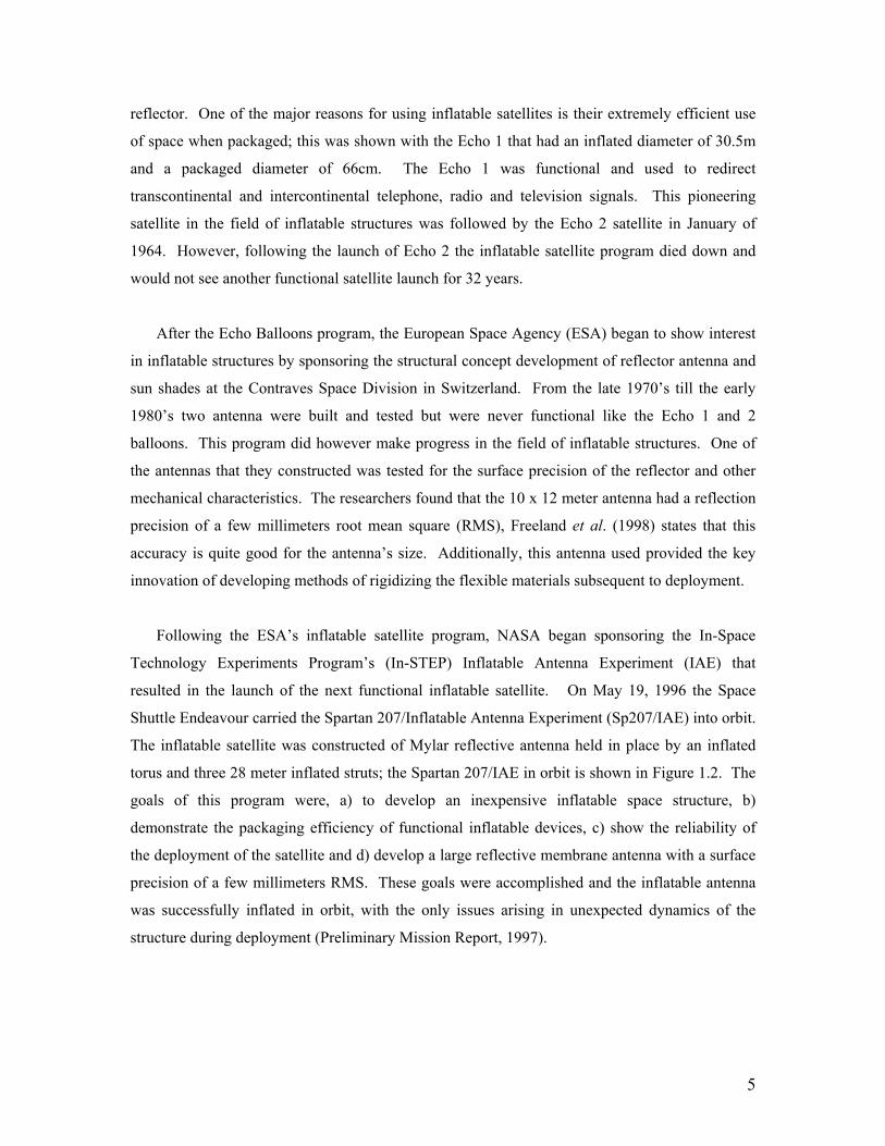
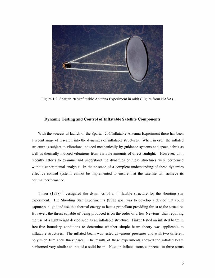
Shuttle Endeavour carried the Spartan 207/Inflatable Antenna Experiment (Sp207/IAE) into orbit.

The inflatable satellite was constructed of Mylar reflective antenna held in place by an inflated

torus and three 28 meter inflated struts; the Spartan 207/IAE in orbit is shown in Figure 1.2. The

goals of this program were, a) to develop an inexpensive inflatable space structure, b)

demonstrate the packaging efficiency of functional inflatable devices, c) show the reliability of

the deployment of the satellite and d) develop a large reflective membrane antenna with a surface

precision of a few millimeters RMS. These goals were accomplished and the inflatable antenna

was successfully inflated in orbit, with the only issues arising in unexpected dynamics of the

structure during deployment (Preliminary Mission Report, 1997).

6

Figure 1.2: Spartan 207/Inflatable Antenna Experiment in orbit (Figure from NASA).

Dynamic Testing and Control of Inflatable Satellite Components

With the successful launch of the Spartan 207/Inflatable Antenna Experiment there has been

a recent surge of research into the dynamics of inflatable structures. When in orbit the inflated

structure is subject to vibrations induced mechanically by guidance systems and space debris as

well as thermally induced vibrations from variable amounts of direct sunlight. However, until

recently efforts to examine and understand the dynamics of these structures were performed

without experimental analysis. In the absence of a complete understanding of these dynamics

effective control systems cannot be implemented to ensure that the satellite will achieve its

optimal performance.

Tinker (1998) investigated the dynamics of an inflatable structure for the shooting star

experiment. The Shooting Star Experiment’s (SSE) goal was to develop a device that could

capture sunlight and use this thermal energy to heat a propellant providing thrust to the structure.

However, the thrust capable of being produced is on the order of a few Newtons, thus requiring

the use of a lightweight device such as an inflatable structure. Tinker tested an inflated beam in

free-free boundary conditions to determine whether simple beam theory was applicable to

inflatable structures. The inflated beam was tested at various pressures and with two different

polyimide film shell thicknesses. The results of these experiments showed the inflated beam

performed very similar to that of a solid beam. Next an inflated torus connected to three struts

7

was tested in ambient conditions with three different inflation pressures, 1.72, 3.45, and 6.89

kPag, in order to characterize the dynamics with a varying internal pressure. An electromagnetic

shaker was mounted to the support plate and used to excite the structure. It was found that the

natural frequencies and mode shapes had considerable change for each different internal pressure.

This test was necessary because as the satellite passes from orbital eclipse to orbital day the

internal pressure could experience significant variations. The inflated torus was also inflated in a

vacuum chamber to determine whether the structure could properly inflate and hold pressure,

Tinker comments that the results were very encouraging.

In later experiments, Slade et al. (2001) tested the dynamics of the inflated torus with three

struts from the Pathfinder 3 Shooting Star Experiment in both ambient and vacuum conditions.

The structure was suspended with free-free boundary conditions and excited using an

electromagnetic shaker attached to the support plate. In order to avoid mass loading of the

structure, a laser vibrometer was used to capture the dynamics. It was found that the natural

frequencies, damping and mode shapes significantly change between ambient and vacuum

conditions. As one would expect the damping of the structure decreased in vacuum conditions.

Slade et al. (2001) state that the results of this study point to a need to conduct vacuum modal

surveys of inflatable articles intended for space application in order to ensure that on-orbit

behavior will be well-replicated in the test environment. Following these tests Leigh et al. (2001)

used the results of the tests performed at ambient conditions to determine the effectiveness of

finite element software to model the inflatable structure. The finite element code

MSC/NASTRAN was used to develop a model of the system for two cases; one using beam

elements and the second using shell elements. The results of the model do not correlate well, but

the authors state that the model shows potential to correlate well, if enough detail is observed

during its creation.

Other recent studies (Agnes and Rogers, 2000) to characterize the dynamics of inflatable

structures have shown to be difficult due to there extremely lightweight, flexible and high

damping properties. The flexible nature of inflatable objects causes point excitation to result in

only local deformations rather than exciting the global modes necessary for model verification

and parameter identification. To overcome these issues Griffith and Main (2000) used a modified

impact hammer to excite the global modes of the structure while avoiding local excitation. The

tip of the impact hammer was enlarged such that sufficient energy was input to the system to

excite the global modes. They found that increasing the internal pressure of the torus from 5.52

8

kPag to 6.89 kPag resulted in significantly less damping and improved the coherence

considerably. During the modal testing the authors used a roving accelerometer technique that

causes differences in the frequency response at each location of the accelerometer due to the

movement of accelerometer’s mass around the system. This is an issue when dealing with

inflatable structures due to their extreme lightweight. One improvement mentioned by the

authors would be to use non-contacting methods of measurements such as a laser vibrometer or

photogrammetry and videogrammetry. A still easier remedy to this problem would be to use a

roving hammer technique, this means that the accelerometer location is stationary and the impact

location is changed.

Smart Materials for Dynamic Testing and Control of Inflatable Satellites

Due to the advances in piezoelectric materials since the early 1990’s smart materials have

become a viable answer to the problems encounter during early testing of inflatable structures.

Some of the issues that were faced with the previously mentioned research into the dynamic

testing of inflatable structures are as follows. Slade et al. (2000) were unable to obtain consistent

results with the laser vibrometer due to a combination of influences of the free-free suspension

system and shaker imposed constraints including mass loading, added damping and non-global

excitation. Griffith and Main (2000) also experienced difficulties including extremely low

coherence and a lack of energy input to the higher frequencies because of the flexible nature of

the inflated object. To overcome these issues many researches have begun to look toward

piezoelectric materials for dynamic testing of inflatable structures.

Agnes and Rogers (2000) attempted to perform a modal test on an inflatable children’s

swimming pool suspended vertically in a square frame. The torus was excited using both an

electromagnetic shaker and Polyvinylidene fluoride (PVDF) patch while the response of the

structure was measured using a laser vibrometer at points around the perimeter of the face of the

torus. The authors used a multivariate mode indicator function (MMIF) to identify the resonant

frequencies. However, further modal analysis was not performed due to significant nonlinear

behavior in the system and low excitation levels on the part of the PVDF patch. Although this

paper did not produce revolutionary results it, it did show that piezoelectric materials could be use

for excitation of inflatable structures.

9

Briand et al. (2000) also used PVDF patches to test the dynamics of an inflatable torus,

although the patches were used for sensing rather than excitation. The test fixture was a tire inner

tube and was excited using an electromagnetic shaker. The experimental setup was able produce

results with good coherence from 0-100 Hz. However, unlike the results found in Agnes and

Roger (2000), a modal analysis was capable of being performed. This was the case because

PVDF patches are ideal for sensing due to their low mass and stiffness, but they are not well

suited for actuation due to low piezoelectric coupling coefficients. The conclusions of the modal

test were then compared to a finite element model with favorable results. The authors also

mention the possibility of using shape memory films and fabrics to produce the actuation energy.

This research showed that smart materials, namely piezoelectrics were a definite choice for

sensing the dynamics of inflatable structures.

Park et al. (2001) used an electromagnetic shaker to excite an inflated tire inner tube with

both accelerometers and multiple PVDF patches located around the structure to effectively sense

the vibration at multiple locations during one excitation period. They found that the data

measured with PVDF film was consistent with that obtained from the accelerometer. Although,

the natural frequencies were almost identical for both methods, those obtained using the

accelerometers were slightly less as expected due to mass loading. However, the PVDF film

sensors offer several advantages when testing inflatable structures because they are lightweight

and extremely flexible allowing them to conform to the torodial shell without adding additional

mass or stiffness to the system. In addition to testing the torus with an electromagnetic shaker

they used both a bimorph PVDF patch and a macro-fiber composite (MFC) to excite the torus. It

was found that the MFC and PVDF patches were ineffective at exciting the lower frequencies but

effective at higher frequencies, this was attributed to imperfect bonding caused by the use of

double sided tape to secure the patches. The PVDF patch used in Agnes and Rogers (2000) was

ineffective while this patch worked well because Park et al. constructed a multilayer bimorph

PVDF actuator that produced far more strain energy than the unimorph patch. One definite

advantage of the smart material actuators over the shaker input was found; they greatly reduced

interference with the suspension modes of the free-free torus. The last portion of this work was to

implement a Positive Position Feedback (PPF) control system using the MFC and PVDF patches

to reduce the vibration of the 3rd and 4th out of plane bending modes. The control system resulted

in approximately 50% vibration reduction, but it is speculated that more attenuation could be

achieved if the actuators were permanently bonded to the structure.

10

Following the work previously mentioned, Park et al. (2002) performed a modal analysis on a

torus constructed of Kapton with an aspect ratio that more closely matched that of the actual

satellites intended for space. The torus was excited with both an electromagnetic shaker and an

MFC actuator. The sensing was performed using both an accelerometer and a PVDF film to

compare the performance of each. It was found that the MFC could globally excite the inflatable

torus and produced better results than the shaker input due to less interference with the

suspension modes of the free-free torus. It was also shown that the PVDF patch provides

measurements of comparable quality to that of the accelerometer. The modal analysis accurately

found the first four out of plane bending mode shapes as well as the first two in plane bending

mode shapes. Ruggiero et al. (2002) used the same test structure to perform a modal analysis

using multiple input and multiple output (MIMO) techniques in addition to developing a PPF

control system to attenuate vibration in the first mode. The MIMO testing techniques are

necessary because multiple actuators would be needed to globally excite the immense structures

intended for space. This work showed that the MIMO testes produce results identical to those

obtained earlier using one MFC for excitation. The MFC was also used to control the first mode

and was shown to reduce the vibration by 70%. However, the authors of this study did not realize

that the controller being used in this case was not applying global vibration reduction but rather

shifting the modes around the symmetric structure of the torus. The shortcomings of the control

system developed by Ruggiero et al. (2002) were identified and improved by Sodano et al.

(2004). Sodano et al. (2004) realized that due to the symmetric nature of the torus repeated

modes were present that cause the use of a signal actuator to suppress one mode while exciting

the other. Therefore, a PPF controller with multiple sensors and actuators was developed and

applied to the torus to correct the issue. The control system was shown effectively suppress the

first mode by approximately 75%, but due to repeated modes and non collocated sensors and

actuators, the higher modes were unable to be controlled. The authors describe a self-sensing

system that would allow the sensors and actuators to be perfectly collocated, but were unable to

implement the system due to the possible instabilities in the analog self-sensing circuit that would

cause surge voltages to be output to the control board, potentially damaging its circuitry.

While much headway has been made in the dynamic testing of inflatable structures, there is

still much to be learned. However, with the advances in piezoelectric actuators, materials,

controls algorithms, finite element programs, structures and computational power of computers,

the steps necessary to understand the dynamics of inflatable devices are becoming clear.

11

1.3.2 Dynamic Modeling, Testing and Control of Membranes

As described in the previous sections, the dynamics of the inflatable structure are particularly

difficult to test and control. While it is necessary that the global structure, i.e. the inflated

components, are dynamically well understood and can be controlled, the overall system will not

function if the membrane mirror or antenna is not dynamically stable. The dynamics of the

membrane pose a whole new realm of testing and control issues. The defining characteristic of a

membrane structure is that it cannot withstand an applied moment and is therefore extremely

flexible. The flexible nature of the structure makes global excitation, for either testing or control

purposes, extremely difficult. When this complexity is coupled with the need for the surface of

the membrane to remain almost perfectly flat in all operating conditions, the task of developing a

satellite that utilizes a large membrane surface is quite daunting. However, the research efforts

put forth in this field have allowed great strides to be made and this technology now appears to be

potentially feasible for optical applications in future space missions. As a note, in the following

section the terminology of an optical membrane also implies use as an antenna.

Theoretical Modeling of Membranes

The concept of utilizing thin membranes for space applications poses numerous complex

modeling issues. For many applications the desired shape of the membrane is parabolic.

However, to achieve this shape, the membrane is typically subjected to either an inflation or

vacuum pressure, often causing surface errors or spherical aberration. The surface aberration is

commonly referred to as a “W-profile error,” which is a measure of the deviation of the actual

surface from that of the desired configuration (Maker and Jenkins 1997). The errors that occur in

these materials can be corrected through control techniques that will be reviewed in a subsequent

section, but the key to any successful control scheme is a theoretical knowledge of the system at

hand. Föppl (1907) developed the equilibrium equation for a membrane plate that are

fundamentally modified von Kàrmàn plate equations (von Kàrmàn, 1910) with the bending

rigidity set to zero. However, in many applications a circular membrane is subjected to a uniform

pressure along its surface, which, as mentioned is a common method of providing a parabolic

shape to the membrane. The first investigation into the solution of a pressurized membrane was

performed by Hencky in 1915, who presented the power series solution to a homogeneous

isotropic linear elastic circular membrane subjected to a normal pressure; this problem became

12

know as Hencky’s problem. These equations saw little interest until the 1940’s when Stevens

(1944) performed an experimental analysis on a 20 in diameter, 0.012 in thick cellulose acetate

butyrate inflated circular membrane. Steven’s compared the membrane deflection results of

Hencky’s with his experiments and formulated an approximation to the shape of an initially flat

pressurized membrane. Over the next three decades Hencky’s problem was studied by various

researchers (Chien, 1948, Shaw and Perrone, 1954, Weil and Newmark, 1955, Cambell, 1956,

Dickey, 1967, Kao and Perrone, 1971, Kao and Perrone, 1972, Schmidt, 1974, Schmidt and

DaDeppo, 1974), however, these studies will not be discussed in this dissertation.

In recent years, modeling techniques for membrane structures have begun to see considerable

attention. Juang and Huang (1983) investigated the analytic solution to the problem of static

shape control using an electrostatically deformed membrane mirror. Their study used large

deformation membrane theory to derive the nonlinear partial differential equations that describe

the control forces necessary to achieve a desired final shape of the membrane. The paper also

presents two examples that illustrate the validity and application of the nonlinear equations of

motion to a membrane of revolution loaded symmetrically by electrostatic forces. Rather than

derive the equilibrium equations, Maker and Jenkins (1997) utilized an FEM program to

demonstrate that the deviation from the desired surface shape can be corrected through boundary

displacements. The results of the analysis show that a maximum deviation of 12.5% is present for

the case of no control and a little over 7% when boundary control is implemented at three

locations, this represents a reduction of 58%. The work of Maker and Jenkins (1997) was

continued by Jenkins et al. (1998), who provide additional FEM results regarding surface control

using boundary displacements. Furthermore a discussion on the relevant surface precision

measurements for an optical surface is provided. Their study showed that by displacing 3 points

on the rim of the membrane by a distance of 4.9 mm, the RMS surface area could be reduced

from 1.43 mm to 0.370 mm. This result is promising because Thomas and Veal (1984) suggest

that the RMS surface error of a membrane reflector should be with 1 mm if the reflector is used in

applications requiring frequencies of less than 15 GHz.

In the first of a series of four papers that develop analytic and FEM modeling techniques for

piezoelectric actuated membranes, Rodgers and Agnes (2002) begin their analysis with a one

dimensional structure, the laminated piezopolymer-actuated flexible beam. Their work provides

a complete development of the nonlinear equations of motion governing the one dimensional

slender membrane material using perturbation techniques. The static response of the beam to the

13

piezoelectric actuator causes a deflection of approximately one wavelength of visible light, which

is stated to agree with experiments presented by Wagner (2000). Furthermore, the deflection of

the beam when subjected to a pressure is presented before and after actuation of the piezoelectric

material. Following the static results, the dynamics of the flexible beam are modeled and the

results are presented. The dynamic solution of the beam shows that when one volt is applied to

the piezopolymer material a deflection of 2.5x10-9 m is achieved. Following the solution of the

one dimensional case, Rodger and Agnes (2002) derived the coupled nonlinear equation of

motion of a piezothermoelastic laminated circular membrane using perturbation techniques.

Using an axisymmetric approximation both the static and dynamic response of the membrane are

analyzed. The static results indicate that the PVDF piezoelectric laminate provide deflection

equivalent to several wavelengths of light. However, the solutions presented are stated to

represent the limit of the analytical approach.

To allow for more complicated membrane systems to be analyzed, Rodgers and Agnes (2002)

introduce the method of Integral Multiple Scales (MIMS) for solving dynamics systems that can

be represented in the Lagrangian Form. The manuscript first develops the integral multiple scales

method and uses it to determine the analytic solution of a beam string. Following the analytic

example, the finite element method is formulated using calculated linear and cubic shape

functions of a beam-string. Once the finite element model was constructed the static and dynamic

results were compared to those of the analytic model. It was found that the use of linear shape

functions caused a fair amount of error, but cubic shape functions were shown to provide high

accuracy of the static deflection. The finite element model was also shown to accurately predict

natural frequencies and the formulas necessary for including damping effects into the model were

provided. Subsequent to the development of the asymptotic finite elements using the MIMS for a

one dimensional structure, Rodgers and Agnes (2003) applied the formulation to the more

complicated two dimensional membrane with discontinuities caused by regions of piezoelectric

material. The method was shown to effectively model the complex interaction of the

piezoelectric and the membrane structure. The banded configuration of the piezoelectric material

was demonstrated to have the greatest effect on the Zernike modes 1, 5 and 13. Furthermore, the

results demonstrate that as the tension in the membrane is increased that the control authority of

the piezoelectric material decreases. Lastly, the forced response is calculated, revealing the

significantly increased dynamic response of the membrane, indicating that the piezoelectric

material may not be the most effective choice for static shape control but very effective for active

vibration control.

14

With the number of modeling techniques growing in the area of membrane theory for optical

and antenna applications, Greschik et al. (1998) published a study that compared the impact on

accuracy of several representative solution approximations on the analytical shape predictions for

both initially flat and curved membranes. The error generated from several different assumptions

and approximations was determined using AM (Axisymmetric Membrane), a highly accurate

numerical solution program that was verified using NASTRAN. This study found the following

result regarding the error caused by solution approximations; higher pressures equate to higher

error, for the linearization methods considered, the small angle approximation causes the most

significant error and ignoring the radial component of Hencky’s solution substantially degrades

the accuracy. Additionally, perturbations were made to the membrane thickness and temperature,

showing that model parameter uncertainties made more significant impact on results than

approximations, while temperature variation degraded the accuracy worse than thickness

variations. Furthermore it was determined that the shallower the parabolic shape, the greater the

error. Because Greschik et al. (1998) was interested in investigating the performance of these

methods at radio frequencies, de Blonk (2003) investigated the shape prediction error for the

higher frequencies required by optical membranes. de Blonk studied three different models, the

axisymmetric membrane shell, axisymmetric large deformation and linear axisymmetric large

deflection. The results showed that all three models performed at the optical level for a range of

non-dimensional parameters but all do not always perform at optical tolerances. These two

studies help define which of the numerous models will work best in a particular application.

Modeling Techniques have made significant progress over the last century and with the increased

computation power available in today’s computers the accuracy of the models will continue to

grow.

Dynamic Testing and Analysis of Membranes

Although the theoretical modeling of membrane structures has made significant progress, the

ability to validate the proposed models through experiments is not an easy task. Marker et al.

(1998) presented an experimental evaluation of the shape limit for a doubly curved membrane.

The test structure for this investigation was a 28 cm diameter, 125 µm thick polyimide film

subjected to a vacuum, causing a 4.47 m concave radius of curvature. Their study applied a

vacuum to the membrane at two locations separated by a ring; the central portion of the

membrane was the first vacuum section and served as the optical portion, while the second area

15

was at the outer ring. The effect of two vacuum areas was to pull the membrane down around the

separating ring, thus causing an increase in the membrane’s prestrain. The surface quality was

measured using a Hartman sensor that detects variance from a flat wave front. The results of the

experimental study showed that an increase in prestrain allowed the optical surface quality to be

improved. Furthermore, it was shown that as the pressure applied to the membrane is increased

the more spherical shaped the surface becomes.

One study performed by Jenkins and Kondareddy (1999) investigated the dynamics of

seamed membranes through both experiments and FEM Analysis, however due to the high

sensitivity to mass, the study did not produce the desired results. The tests were performed on a

1-mil thick membrane with a diameter of 6.82 in, with seams simulated by bonding 0.5 in strips

of the membrane material to the structure. To measure the dynamic response of the simulated

seamed membrane a laser Doppler vibrometer was used. Three experiments were performed to

identify the effect of seams on the membrane dynamics, the fist had no seam, the second had

seams at 90 degrees and the third had seems at 45 degrees. The results showed that the natural

frequency dropped significantly due to the addition of the membrane strips. The drop in resonant

frequency indicates that the strips caused mass loading and not additional stiffness as intended.

This result shows that the membrane strips did not correctly simulated the stiffness added by

actual seems, thus demonstrating the difficult testing nature of the membrane structure.

The Air Force Research Laboratories have performed extensive research into the testing and

improvement of optical membranes. One study performed by Rotgé et al. (2000) at the

membrane mirror laboratory, investigated two methods of improving the surface quality. The fist

method described in the paper was to develop more suitable membrane materials. The authors

describe a recently developed type of polyimide film called “CP-N.” The authors state that this

material, which has a surface flatness of 0.05 λ rms (where λ rms is the root mean square of the

wavelength of optical light), may be the key solution necessary to develop a functioning

membrane mirror. The material was tested by constructing a 28 cm diameter test bed and

measuring the surface flatness an optical quality. It was determined that once the membrane was

fixed the surface flatness was approximately 30 λ rms with a blur circle 14 mm in diameter. By

increasing the vacuum pressure the size of the blur was reduced from 14 mm down to 3 mm. The

second method used to improve the optical quality of the membrane was Real Time Holography

(RTH). The RTH method takes the optical image and processes it to improve the quality. Using

RTH the blur size was reduced from 6 mm down to 120 µm or approximately 1-2 λ rms. This

16

demonstrates the ability of RTH to correct for the surface error in a stretched membrane optical

surface. Data processing techniques such as RTH are important to membrane testing because

they allow for greatly decreased surface and structural tolerances.

Like the research performed at the Air Force Research Laboratories, Hiroaki and Yuma

(2001) studied a method to manufacture higher surface quality materials. The authors constructed

a 115 µm thick membrane out of plastic reinforced triaxial fabrics woven with aramid fiber and

Poly-Phenylene Benzobisoazole (PBO) fiber and stretched in inside of an inflated torus.

However, this study was interested in testing the material’s surface characteristics for use in

antenna applications, which have a surface tolerance far more relaxed than that of an optical

surface. The 1.5 m inflated torus used was shown to be capable of being very compactly

packaged in a cylindrical shape with a height of 380 mm and a diameter of 300 mm. Using a

scanning laser vibrometer their study found that after being packaged and deployed the surface

flatness was better than 0.1 mm rms when stretched with a tension of 28.9 N at 24 tensioning

points. Studies that demonstrate the packaging, deployment and antenna surface quality after

deployment are extremely important to the success of inflated devices. This research has

demonstrated all three important aspects of the inflated structure, as well as, developed a

membrane material that after being deployed from its packaging is well below the surface

tolerance required by antenna for space applications.

CSA Engineering has published a series of papers that investigate the dynamics of

membranes in both ambient and vacuum temperatures. In 2001, Flint and Glease (2001)

performed experiments and FEM analysis on a tensioned hexagonal membrane. The study

characterized the Young’s Modulus and loss factor over a range of frequencies from 10-80 Hz

and found Kapton’s stiffness to increase by 1.2% and the loss factor to increase by 10% over the

tested frequency range. Following these experiments dynamic tests were performed and the

results were compared to those calculated using the FEM program NASTRAN and were shown to

match well. Lastly this study investigated the addition of constrained layer damping treatments to

the membrane surface. Results from these experiments varied, in certain cases the damping was

actually decreased, while the best result showed the damping to increase from 1.5% to 5.2%,

however, the mass in this case was raised by over 4.5 times. In a subsequent study, Hall et al.

(2002) modeled and tested 2-mil Kapton membrane strips. The study found that FEM models

could accurately predict the response of the strip, however, particular attention to the boundary

conditions during testing was required to obtain good results.

17

Continuing CSA Engineering’s research, Bales et al. (2003) studied the effects of thermal

variations, hydroscopic changes and vacuum pressure on the preload tension and dynamic

response of a 2-mil thick Kapton strip. These experiments found some interesting results. It was

determined that the thermal effects of the membrane tension were hard to quantify due to the

thermal expansion and contraction of the metal test structure, but they did show that the tension

was highly dependent on the surrounding temperature. While the structure interfered with the

thermal experiments, the metal components of the structure did not have any hydroscopic

characteristics, allowing these tests to be accurately performed on only the membrane material.

During the experiments the relative humidity was varied from 35% up to 100% and back down to

35%. It was found that as the humidity increases, water is absorbed into the Kapton material

causing the material to expand and the tension to decrease, as the humidity decreases the water

evaporates out of the material causing the tension to increase significantly. The last experiment

performed looked at the changes in dynamic response as the pressure is reduced to vacuum. The

study found that the resonant frequencies shift dramatically from 44 Hz at atmospheric pressure

to 52 Hz at vacuum, representing a 20% increase. The increase in natural frequency occurs

because as the pressure decreases to vacuum, the water content of the Kapton specimen is

expelled causing the material to shrink and the tension to increase. Additionally, the damping is

significantly lower at vacuum pressure. In the most recent study, Flint et al. (2003)

experimentally tested the dynamics of a 0.5m and 1.0m diameter doubly curved mirror made

from 52 micron thick Kapton at atmospheric pressure, vacuum pressure and in a nitrogen

environment at several different pressures ranging from 100 torr to 690 torr. The experimental

results of the tests showed that the doubly curved membrane was very difficult to test and the

experimental configuration did not allow all of the modes to be excited. Although the results

were not definitive, it was shown that the dynamics of the ring were significantly changed at

vacuum and that hydroscopic effects did not present any noticeable change in the dynamic

response. Additionally, before testing rough calculations were made to predict the dynamic

response of the membrane, however, the estimated natural frequencies did not match the

measured data well.

The experimental tests performed by researchers at CSA Engineering used a laser vibrometer

to measure the dynamic response of the membrane structure. A second method of measuring the

dynamic response of an extremely flexible structure is the use of photogrammetry and

videogrammetry, which has been investigated thoroughly by researchers at the NASA Langley

18

Research Center. Perhaps the first in a series of publications on the topic was Pappa et al. (2001),

which investigated the ability to use consumer digital cameras for photogrammety in the analysis

of a 5m inflated space antenna. The work presents a basic introduction into photogrammetry and

provides an eight step formula to generate the static shape of the antenna surface. The eight steps

are: 1) calibrate the cameras, 2) plan the measurements, 3) take the photographs, 4) import the

photographs into analysis software, 5) mark the target location in the software, 6) identify the

same points in each cameras frame, 7) process the data, and 8) export 3D coordinates to a CAD

program. Using the above steps, a single picture from four 2.1 megapixel digital cameras and

500 retro-reflective points mounted to the structure, the authors were able to measure the static

shape of the structure to within 0.02 inches in-plane and 0.05 inches out-of-plane. In a later

study, Pappa et al. (2002) discuss a more advanced procedure for determining both the static

shape and dynamic response of ultra flexible structures. Seven successful test specimens are

discussed and sophisticated cameras and dot projectors are used. To compliment these studies,

Dharamsi et al. (2002) compared the photogrammety method with the capacitance sensor, a

proven method for measuring the characteristics of a membrane. Their study found that the

accuracy of both methods matched astonishingly well, the equipment needed to perform

photogrammerty cost about one third of the price of a capacitance measurement system and the

time required to measure and process the data was a fraction of that needed for capacitance

systems. However, when using retro-reflective targets and white-light dot projection techniques

it can be difficult to provide enough data points for the photogrammertry system to provide a

detailed account of reflective and transparent membranes. To account for such limitations, Pappa

et al. (2003) discuss the laser-induced fluorescence method of dot projection. This method uses

polymer materials that have been manufactured with a small amount of dye in them such that

when excited by a laser light source the dye absorbs a fraction of the laser energy and

consequently fluoresces at a longer wavelength. This method provides a means of projecting a

high density pattern on the surface of materials that with other techniques would require

significant exposure times, eliminating the ability to perform dynamic testing. The method of

laser-induced florescence videogrammetry was compared to laser vibrometer by Blandio et al.

(2003). However, it was found that the laser vibrometer was superior in all aspects other than

cost, which is significantly greater. During testing the vidiogrammetry technique identified

modes that were not present and could only be used below 5 Hz because of camera limitations.

For thin membranes to be used in space, ground testing techniques are of utmost importance.

The publications presented in this section are only a fraction of the many investigations into

19

experimental studies and techniques for ultra lightweight and ultra flexible structures. With the

advances being made in this area and the collection of research papers, ground testing of these

structures is now a feasible goal.

Control Methods for Optical Membranes

After a structure is thoroughly understood through modeling and experimental testing control

schemes can be developed to improve the systems performance. The idea to develop an adaptive

membrane for use as an optical surface is not a new concept and has been looked at by numerous

research groups. In 1977, Grosso and Yellin tested an adaptive optical membrane and presented

the basic design equations to determine the membrane’s optical performance. The test specimens

were 50 mm diameter titanium and nickel membranes of various thicknesses and the adaptive

system was constructed using 53 individual hexagonal electrostatic actuators. It was found that

one actuator located a distance of 50-100 µm away from the membrane could generate a typical

deflection of one half a wave with less than 100 volts applied and a deflection of several waves

when numerous actuator were used. The experiments performed, investigated the fundamental

frequency of the each sample as a function of pressure and it stability over time as well as the

deflection of the membrane when actuated. It was found through the experimental results that the

design equations provided a very accurate prediction of the systems performance.

During the late 1970’s the idea of constructing an adaptive membrane optical surface saw its

first patent by Perkins and Rohringer (1978). The patent was issued for an adaptive optical

membrane that utilized multiple electrostatic actuators to both statically deflect and dynamically

control the surface of the membrane for optimal performance. It is stated that all other work prior

to this utilized only a single electrode to statically deform the membrane. Perkins and Rohringer

(1978) also discuss two methods of sensing the optical quality of the membrane surface. The first

method uses a laser range finder or a multipoint interferometer to determine the position of the

membrane, and then correct it using closed loop feedback control. The second device discussed

is an optical sensor that is placed at the focal plane of the membrane mirror and then supplied to a

processor that can detect the deviation from the desired optical quality of a portion of the mirror

allowing feedback control to be applied to that area. More detail on optical sensors of this kind is

discussed by Muller and Andrew (1974).

20

Research into membranes for optical surfaces was a small field yet continued to grow into the

1980’s and early 1990’s. Like Grosso and Yellin (1977), electrostatic actuators were used by

Claflin and Bareket (1986) to generate shape functions on the surface of the membrane mirror.

Their study investigates an approximate analytic solution of Possion’s equation that allows the

determination of the influence functions for a circular electrostatic mirror. With the influence

functions known, a fitting procedure can then be used to obtain the optimal voltage setting for

each electrostatic actuator such that the desired shape can be reproduced on the membrane

surface. The process is demonstrated on a circular membrane mirror developed by Merkle et al.

(1981) that utilized 109 electrostatic actuators and is shown to be capable of reproducing Zernike

Polynomials up to degree six with good accuracy.

Takami and Iye (1994) proposed and constructed an adaptive membrane mirror for the

Cassegrain adaptive optics of SUBARU, an 8 m telescope at Mauna Kea in Japan. For the

SUBARU project two types of adaptive mirrors were investigated. The first was a bimorph

mirror made of two plates of piezoelectric material linked together and covered by a thin silicone

shell that acts as the optical surface. The surface curvature of the mirror is modified by applying

a voltage to both sides and utilizing the piezoelectric effect (Jagourel et al. 1990). However, this

configuration was not focused on because of the complexity of polishing the bimorph mirror.

The second concept used a mirror made of a 2 µm thick aluminum coated nitrocellulose

membrane with a diameter of 50.8 mm and an effective area of 25 mm diameter. The aluminum

surface of the mirror was used such that it was reflective as well as conductive, thus acting as a

bias voltage electrode. Actuation of the mirror was accomplished through the use of 25

electrodes located 530 µm from the surface. The drawback of the membrane mirror was that for

operation of the control system, a vacuum chamber was required to avoid discharge of the

electrodes. Through experiments it was determined that the optical surface quality of the

membrane was 0.03 λ rms inside the 25 mm effective area and was present up to the near infrared

region (tests were limited to the near infrared region because of the glass window used on the

vacuum chamber). During testing of the membrane, it was found that when the membrane was

operated at vacuum pressure the damping was very low causing large resonant peaks beginning at

1.6 kHz, thus limiting the operation of the mirror. To correct this problem it was found that if the

pressure was increased to 5 Torr the damping was significantly improved and electrical discharge

was avoided.

21

With the improvements in materials, computers, manufacturing techniques and the successful

launch and deployment of an inflated satellite in 1996, the late 1990’s saw a surge of research

into the area of optical membranes. During this time period a number of interesting alternative

control schemes were developed. One such alternative approach to control the surface precision

of optical membranes was proposed by Divoux et al. (1998), who developed the concept of using

a membrane coated with a magnetic layer that could be actuated by numerous micro-coils. The

study used three finite element packages to investigate the effect of both 2 mm and 6 mm coils on

the 30 mm membrane. A prototype of the 25micro-coil array was constructed with 6 mm

diameter and 3 µm thick aluminum conductors. However it was found that the resistance of the

aluminum coils was too high and excessive heating was present. To overcome this issue Cugat et

al. (2000) used a LIGA (German acronym meaning, lithography, electroplating and molding) to

construct a hexagonal array of 19 coils with a diameter of 6 mm and 80 µm thick electrodes.

Using this micro-coil array, experiments were performed on a membrane with 19 samarium

cobalt (SmCo) permanent magnets glued to the surface resulting in a static deflection of 15 µm,

the system was also able to dynamically perform up to 200Hz.

Another approach to non-contact shape control of membrane mirrors was performed by Main

et al. (1999) using an electron gun to excite a piezoelectric patch. By applying an electric

potential to one side of the piezoelectric material and firing the electron gun at the other side, a

surface charge is developed that can be varied with the intensity of the electron beam. Using this

technique, the strain of the piezoelectric material can be controlled while alleviating the need for

an electrode pattern and the limitations that are imposed by them. The study first tests a

piezoceramic plate to determine the excitation behavior of the electron beam and to understand

the relationship between applied field and electron guns strength. Next a bimorph PVDF

cantilever mirror was tested to determine the deflection that could be induced in the piezoelectric

polymer. The results found that using this technique the tip of a 10cm long beam could be

deflected 4mm. It was also shown that discrete areas of the beam could be excited using the

electron beam.

Rather that using an electron gun to excite regions of a PVDF membrane, Wagner et al.

(2000) studied the ability to bond a layer of PVDF film to a membrane and apply active control to

select regions with various electrode patterns. The authors provide a very detailed account for the

construction of a 125 µm thick UPILEX membrane (an average surface roughness of 3 nm) along

with the procedure used to etch an electrode pattern onto 52 µm thick PVDF and the methods

22

used to bond it to the membrane surface. Four mirrors were constructed to investigate the surface

quality of the membrane, the first had no PVDF material bonded, the second was completely

covered by PVDF material, the third had a square region coated and the fourth had four square

PVDF patterns. It was found that the membrane with no PVDF bonded to it optically performed

the best with a 4.5 µm deviation in surface flatness. The other three membranes with PVDF

material attached were excited with varying voltages to determine the effect of the PVDF control

patches. It was shown that motion of 32 µm was achieved with excitation of the PVDF patch.

This study illustrated that the PVDF material could be bonded to the surface of the membrane and

potentially be used for active control of the optical surface. However, because of the bonding

condition between the PVDF and the membrane the optics were degraded rather than improved,

once again pointing out the sensitive testing nature the membrane.

A follow up study to Wagner et al. (2000) was performed by Sobers et al. (2003), who

constructed two PVDF membrane mirrors that had different etched electrode patterns in order to

control regions of the piezoelectric material. Once the membrane mirrors were fabricated, the

surface flatness was measured and shown to be 1.2λ RMS and 0.63 λ RMS for the first and

second mirrors, respectively. Using the PVDF layer control voltages were applied to selected

actuators and the surface flatness was shown to be reduced to 0.87λ RMS and 0.27 λ RMS, for

the first and second mirrors, respectively. Additionally, the piezoelectric actuators were used to

deform the membrane into Zernike polynomials and showed that the separate electrode regions

only deformed the actuated regions indicating that high-order surface control was achieved. The

results indicate that the use of PVDF film for control of optical membranes can provide

corrections to surface flaws and may be usable in space in the near future.

Solter et al. (2003) also used smart materials to actively suppress the vibrations of a

membrane, however, their study used a piezoelectric stack actuator and two macro-fiber

composite patches to actively adjust the in plane tension and out of plane displacement from the

boundary of the membrane. The structure tested was a rigidized hexapod with a 1mil thick

Kapton membrane tensioned in the center by 12 cables. For this study one of the cables was

replaced by the piezoelectric actuator. The stack actuator was responsible for adjusting the

tension of the active cable and the macro-fiber composite was used to deflect the cable out of

plane. Using this actuation system a lead-lag compensator was build to reject the disturbance of

the membrane above 15Hz. The system was shown to be effective in reducing the magnitude of

the response at the resonant peaks, even with limited tension control from the piezoelectric stack.

23

The literature that has been presented in the area of membrane modeling, testing and control,

clearly shows the complex nature of the extremely flexible structure. While significant advances

have been made is this field, the use of membranes in space for optical or antenna purposes is a

goal that is not yet attainable. However, with the renewed interest in ultra large, ultra lightweight

space devices, there has been a surge of research into membranes. These increased research

efforts, will surly provide the advances necessary to develop a membrane system capable of space

missions.

1.3.3 Eddy Current Damping

This dissertation will investigate the ability to use the eddy currents generated by magnetic

fields to suppress the vibration of the ultra flexible devices intended for space. The eddy current

phenomenon is caused when a conductive material experiences a time varying magnetic field.

This time varying magnetic field can either can be induced either by movement of the conductor

in the field or by changing the strength or position of the source of the magnetic field. The

generated eddy currents circulate such that they generate a magnetic field of their own, however

the field generated is of opposite polarity as the change in flux, causing a repulsive force.

However, due to the electrical resistance of the metal, the induced currents will dissipated into

heat at the rate of I2R and the force will disappear. In the case of a dynamic system, the

conductive metal is continuously moving in the magnetic field and experiences a continuous

change in flux that induces an emf, allowing the induced currents to regenerate and in turn

produce a repulsive force that is proportional to the velocity of the conductive metal. This

process causes the eddy currents to function like a viscous damper and dissipate energy forcing

the vibrations to die out faster.

The generated eddy currents can be potentially used for many interesting dynamic

applications. In the following section, previous studies using eddy currents for dynamics systems

will be presented. The concept of using eddy currents for damping purposes has been known for

a considerable time, with manuscripts dating to the late 1800’s, therefore, the history of the eddy

current damper will not be presented and only work from the past few decades will be reviewed.

First, eddy current braking systems will be discussed; this is the most common and well

developed application of eddy currents, subsequently the use of eddy currents for the suppression

24

of rotor vibration will be detailed, and lastly research into eddy currents used to damp structural

vibrations will be reviewed.

Eddy Current Braking

Eddy current breaking typically uses the rotational movement of a conductive medium

between two oppositely poled magnets to induce an emf in the material. A schematic showing

this concept is provided in Figure 1.3. By configuring the two oppositely poled magnets as

shown in Figure 1.3, the magnetic field is concentrated in the gap between the two magnet

surfaces, therefore causing the conductive material passing through this region to experience the

maximum change in magnetic flux and thus induce the greatest eddy currents and damping force.

For this reason, the arrangement of the magnets and conductor’s motion as shown in Figure 1.3

provides the optimal eddy current damping system. For magnetic breaking purposes, this

configuration fits the system well and has been investigated by numerous researchers. One early

study into eddy current breaking was performed by Davis and Reitz (1971), who examined the

forces induced on a magnet moving over the surface of both a semi-infinite and a finite

conducting medium. Their research utilizes an image concept proposed by Sommerfeld (1889) to

allow the induced eddy currents in a finite conducting disk to be calculated. The results provide

the Green’s functions that were unable to be calculated by Sommerfeld (1889) and propose an

approximate solution to the case of a finite dimension conducting sheet of finite conductivity,

which causes difficulties in the solution due to the decay in eddy current density from joule

heating. Later, Schieber (1974) analytically predicted the braking torque on a finite rotating

conductive sheet and performed experiments to identify the accuracy of the modeling techniques.

The results showed that the model and the experiments were in good agreement, however, it is

speculated that the use of an over simplified magnetic flux density over the magnet’s projected

pole was responsible for degraded results. Additionally, the study used the experimental setup

and model to determine the optimal radial placement of the magnet and found it to be in

agreement with results presented in previous research, thus indicating the functionality of the

experimental setup and accuracy of the model. Subsequent to this study Schieber continued his

research in eddy current breaking and published a paper in 1975 that analytically found the

optimal size of a rectangular electromagnet for eddy current braking. However, the braking force

was not applied to a rotating disk but rather to an infinitely large plate and an infinitely long beam

moving between the two magnets. His study found that the optimal ratio of the length to the

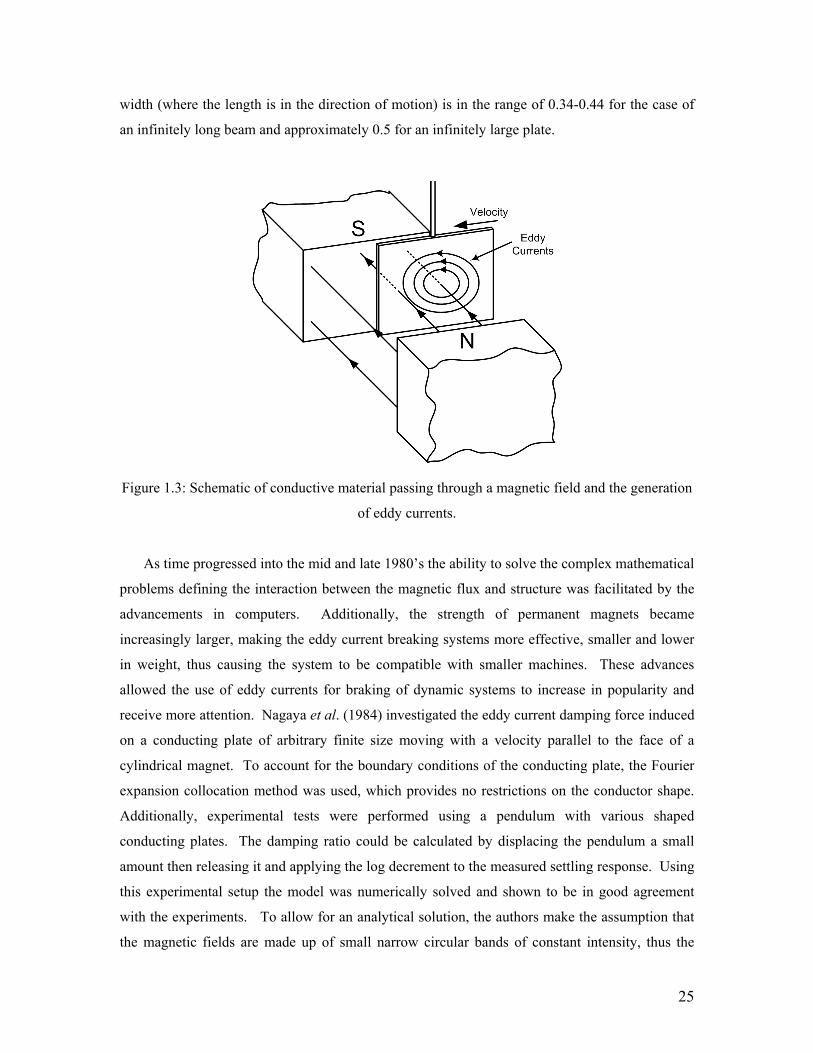
25

width (where the length is in the direction of motion) is in the range of 0.34-0.44 for the case of

an infinitely long beam and approximately 0.5 for an infinitely large plate.

Figure 1.3: Schematic of conductive material passing through a magnetic field and the generation

of eddy currents.

As time progressed into the mid and late 1980’s the ability to solve the complex mathematical

problems defining the interaction between the magnetic flux and structure was facilitated by the

advancements in computers. Additionally, the strength of permanent magnets became

increasingly larger, making the eddy current breaking systems more effective, smaller and lower

in weight, thus causing the system to be compatible with smaller machines. These advances

allowed the use of eddy currents for braking of dynamic systems to increase in popularity and

receive more attention. Nagaya et al. (1984) investigated the eddy current damping force induced

on a conducting plate of arbitrary finite size moving with a velocity parallel to the face of a

cylindrical magnet. To account for the boundary conditions of the conducting plate, the Fourier

expansion collocation method was used, which provides no restrictions on the conductor shape.

Additionally, experimental tests were performed using a pendulum with various shaped

conducting plates. The damping ratio could be calculated by displacing the pendulum a small

amount then releasing it and applying the log decrement to the measured settling response. Using

this experimental setup the model was numerically solved and shown to be in good agreement

with the experiments. To allow for an analytical solution, the authors make the assumption that

the magnetic fields are made up of small narrow circular bands of constant intensity, thus the

26

exact magnetic density over the whole surface of the conductors with a complicated shape could

not be considered. They state that due to this assumption, the model is only accurate for

conductors of which the area is about ten times the cross sectional area of the magnet.

Furthermore, the authors assume that the eddy currents generated through the thickness of the

conductor are zero because of the conductor’s small thickness. However, through experiments it

was found that this assumption is only valid for conductors with a thickness under of 5 mm.

Wiederick et al. (1987) proposed a simple theory for the magnetic braking force induced by

eddy currents in a thin rotating conductive disk passing through the poles of an electromagnet.

Their model found the damping force to be linearly related to the velocity, conductivity and air

gap, but quadratically dependent on the magnetic flux. The proposed model does not consider the

effects of the edges of the conducting plate and while the paper provides an experimental study, it

does not validate the accuracy of the model well. Additionally, when formulating the model the

authors made two assumptions; that the infinite disk is moving linearly rather than rotating and

the eddy current density within the rectangular “footprint” of the electromagnet is uniform and

zero elsewhere. Subsequent to the publication of Wiederick et al. (1987), Heald (1988) took the

model proposed by Wiederick et al. (1987) and formulated expressions that alleviated the need to

assume a constant eddy current density in the “footprint” of the electromagnet and zero

elsewhere. The results of the improved model were compared to those found by Wiederick et al.

(1987) and were shown to increase the accuracy from 96.3% to 99.4%.

Rather than study the effect of eddy currents on a rotating system, Cadwell (1995)

investigated the breaking force exerted on an aluminum plate as it passes between the poles of a

horseshoe electromagnet. A simple model of the system was developed that leaves the length of

the eddy currents path as an unknown parameter, which is fit using the experimentally obtained

results. By adjusting the length of the eddy current, the damping force induced on the aluminum

plate can be varied. Due to the use of a fitting parameter, the true accuracy of the model is not

presented in the authors results. Experiments were performed by sliding a cart with a vertical

aluminum plate attached down an air track. The position, velocity and acceleration of the cart

were measured to determine the damping force applied to the cart as it passed between the poles

of the electromagnet. After performing the experiments the authors found the length of the eddy

current path to be slightly less than the vertical height of the effective magnetic field.

Additionally, it is stated that the magnitude of the eddy current was over 1000 Amps, but the

27

resistance of the path taken is only 3.5x10-6 Ohms, thus resulting in a power dissipation of 12

watts.

As the modeling techniques for eddy current braking processes improved in accuracy, control

techniques could be used to adjust the braking force of the system. One such controller was

designed an implemented by Simeu and Georges (1996) to actively vary the intensity of the

electromagnet and thus control the speed on the rotating system. This study uses the idea

discussed by Wouterse (1991) that the eddy current brake’s behavior falls in one of three regimes.

The low speed region when the magnetic induction caused by the eddy current pattern is

negligible compared to the original induction and the air gap magnetic induction is then slightly

less than that generated at zero speed, the critical speed region is the speed zone at which the

maximum drag force is exerted and the induction caused by the eddy current pattern is no longer

negligible compared with the zero speed induction, and lastly the high speed region, were the

mean magnetic induction in the air gap tends to decrease further and as the speed increases to

infinity the original magnetic induction will be completely canceled out by the induced eddy

currents. Using the first of the three different behavior regimes (low speed), static and dynamic

feedback compensator schemes were proposed and implemented to control the speed of the

rotating disk in the presence of an unknown varying braking resistance torque. The results

showed that by varying the eddy current braking force the speed of the rotating wheel could

accurately follow a reference speed even in the presence of a disturbance torque. Additionally, it

was demonstrated that both control schemes functioned well, but the dynamic feedback controller

was more effective than the static.

Lee and Park (1999) also investigated the design of an eddy current brake controller.

However, their system was not intended to maintain a fixed speed, but to minimize the stopping

time. The authors suggest that for the control system to be applicable to an automobile braking

system, it should have the ability to apply a braking force that is dependent on different road

conditions. Therefore, a sliding mode controller was designed to allow the maximum braking

force to be adjusted depending on the road condition. After modeling the eddy current braking

system, the control scheme was simulated. The results of the simulation showed that the braking

system performed very well in the high speed region, but the eddy current damping force is

proportional to velocity, so as the speed decreases the current applied to the electromagnet must

be increased. Once the current was raised to the saturation level of the electromagnet, the braking

performance fell off quickly. However, the authors state that the average deceleration before

28

saturating the electromagnet was 0.8 g, which is higher than the 0.5 g value suggested by the

National Association of Australian State Road Authority. The simulation was then compared to

experiments that measured the stopping time of a rotating conductive disk. It was shown that the

laboratory simulation and model matched very well. In the high speed range, the performance of

the eddy current braking system was shown to be superior to the hydraulic brakes typically used

in automobiles because of a fast response time and due to their non-contact nature, they alleviate

the need for regular maintenance. This paper shows that in the high speed region the eddy current

baking system is feasible for use in an automobile, however, it would be necessary to have a

hydraulic system in the low speed region.

More recently, Lee and Park (2001a, 2002b and 2002) developed a model for an eddy current

braking system that allows for an analytic solution to the problem. The model allows for one or

more separate magnets to apply a magnetic field to the rotating conductor. The electric field

intensity was first computed then the concept of the mirror image was introduced to account for

the edge effects caused by a finite radius of the rotating disk. The image method works by taking

the predicted eddy current density and rotating it about the edge of the conductor to create an

imaginary eddy current density that is then subtracted from the originally predicted density to

arrive at a net eddy current density. The authors use a lumped formulation of the radial

component of the eddy current density in the pole projection area and neglect the tangential

component for the net eddy current density. It is stated that the tangential component is expected

to be smaller than the radial component and therefore only the radial component is included for

convenience. To obtain the expression for the net eddy current, the radial component of the eddy

current density was numerically integrated. Additionally, the magnetic Reynolds number (the

ratio of induced magnetic flux to the applied magnetic flux) was used with the expression of the

net magnetic flux density assumed to be an exponential function. The applied braking force and

torque was then calculated and the model was compared to experimental results. It was found

that the model compared very well to the experimental results, with some discrepancy occurring

when multiple magnetic sources were placed in close proximity. The errors are believed to be

caused by calculating the total net magnetic eddy current in one pole projection area without

including the effects on the magnetic Reynolds number from other pole projection areas.

29

Magnetic Damping of Rotor Vibration

A second application of eddy current damping with rotational systems is the suppression of

lateral vibrations of rotor shafts. A major source of rotating equipment failure occurs due to

slight imbalances in the rotor causing self excitation. The magnets in the eddy current dampers

used for the suppression of rotational vibrations are configured in the same manner as those used

in magnetic braking applications. Gunter et al. (1983) investigated the design of an eddy current

damping system for the cryogenic pumps used to deliver the liquid fuel to the main engines of the

space shuttle. These pumps are susceptible to subsynchronous whirl, which can be extremely

destructive and has been responsible for bearing failures and severe rubs in the seals, resulting in

premature engine shutdowns and limited operation of the turbo pumps. The authors used the idea

that at the very low operating temperature of the cryogenic pumps the resistively of the conductor

is decreased allowing larger damping forces to be generated. The damping concept was modeled

using a rough finite element code and the damper’s performance was estimated. The authors state

that the damping generated by the system was sufficient to help suppress the rotor vibration,

however results presented are hard to decipher.

Like Gunter et al. (1983), Cunningham (1986) studied the use of eddy current dampers to

suppress the lateral vibration experienced by the cryogenic turbomachinery use in space shuttles.

Three magnet/conductor combinations were tested on a rotor operated between 800 and 10,000

rpm with the damping mechanism completely immured in liquid Nitrogen. The experimental

setup was constructed and tests were performed to determine the damper’s performance. Using

three different sized magnets it was shown in the best case that the damping coefficient could be

increased from 70 to 500 Nsec/m in the X-direction and from 110 to 320 Nsec/m in the Y-

direction. The increase in damping coefficient was also calculated using theoretical analysis to

provide an average accuracy of within 28.7% in the X-direction and 10.7% in the Y-direction.

Frederick and Darlow (1994) looked at using an eddy current damper to replace the coulomb

or squeeze film dampers typically used in rotating machinery, whose damping properties

typically change with temperature and cause additional torque loading and wear. The damping

system consisted of a horseshoe electromagnet that had a conductive disk rotating between the

magnetic poles. The study was purely experimental and showed that the peak to peak response

was reduced in the X-direction by 15.6% and in the Y-direction by 27.5%. While the results of

the experiments are feasible, the authors state that the damper does not cause any rotational

30

loading. This comment seems to be completely incorrect because the configuration of the

damping system does not differ from a magnetic braking system at all, and therefore must

produce a drag force on the rotation of the disk.

Kligerman et al. (1998a, 1998b) and Klingerman and Gottlied (1998) published a series of

papers investigating the instability in rotor dynamics caused by the use of electromagnetic eddy

current dampers. The first study of the series (Kligerman et al. (1998a)) theoretically and

experimentally showed that eddy current dampers are not effective for use in rotating systems that

are operating in the supercritical range because the dampers can induce unstable operation.

However, it is stated that the eddy current damper does form an effective vibration reduction

mechanism for subcritical operation. The authors state that the instability is caused by the

rotation of the conductive disk in the magnetic field and that if the rotation of the disk can be

eliminated the damper would function throughout all operating conditions. To validate this

statement, an experiment was performed where the rotating disk was detached from the shaft and

mounted to a bearing, thus allowing the disk to spin freely. Due to the eddy current braking

effect, the disk’s rotation was almost completely eliminated allowing the authors prediction to be

tested. The test results showed that indeed the rotation of the conductor between the magnets was

responsible for the destabilizing effect and that the damper’s effectiveness improved with an

increase in current applied to the electromagnet. The stability of the shaft with a freely rotating

conductor was evident through the supercritical range.

Klingerman et al. (1998b) continued his research into rotating systems with eddy current

dampers by studying the systems stability with a non-linear cubic restoring force at the shaft

supports. Through a numerical analysis it was determined that the rotating system goes unstable

via a Hopf bifurcation when a specific supercritical angular velocity is reached. The frequency

threshold for instability is provided and is related to the magnetic damping coefficient, the system

damping coefficient and the natural frequency of the shaft. The analysis also provides a closed

form solution for the radius of the limit cycle. Furthermore, the study found that in low speed

operation the forced unbalanced response consists of periodic vibration corresponding to the

systems rotational frequency, but high speed operation was shown to be governed by coexisting

quasiperiodic solutions. Later, Klingerman and Gottlieb (1998) determined that the influence of

nonlinear damping is negligible near the stability threshold.

31

The use of an active control system to suppress the lateral vibration of a rotating system was

studied by Fung et al. (2002). A rotating shaft with circular disks was analyzed using the

Timoshenko-beam model and Euler-beam model to determine the effectiveness of three control

algorithms; quadratic, nonlinear and optimal feedback, for vibration suppression of the shaft. It

was found that nonlinear feedback control provided the best settling time and that optimal

feedback control generated the smoothest control current input. For the system studied, it was

determined that the eddy current damper could be used to suppress the flexible and shear

vibration simultaneously and that system remained asymptotically stable.

Eddy Current Damping of Structural Vibrations

While the single most prominent application of eddy currents for suppressing dynamic

motion has come in the form of magnetic braking, numerous studies have been performed that

utilize eddy current damping for the suppression of vibrations in a range of applications. The

following section will not concentrate on a single application, but will detail some of the many

research applications that have been performed in the area of magnetic damping.

Karnopp (1989) introduced the idea that a linear electrodynamic motor consisting of coils of

copper wire and permanent magnets could be used as an electromechanical damper for vehicle

suspension systems. The study presented the ability to use a moving coil and a moving magnet

actuator as the damping mechanism and employed some rough calculations to identify the system

performance; however no experiments were performed to validate the calculations. The author

showed that his actuator could be much smaller and lighter than conventional actuators while still

providing effective damping in the frequency range typically encountered by road vehicle

suspension systems.

Kienholz et al. (1994) developed a tuned mass damper vibration absorber to suppress the

vibration of a solar sail array. The frequency range of interest was from 0.1-1.0 Hz, thus the

spring element of the system was required to have a very low stiffness and large stroke. Because

the stroke of the absorber was very large (8 in) and most dampers would add stiffness to the

structure, the choice of damping mechanism was difficult. The solution was the use of magnetic

dashpots that were constructed with two shallow horseshoe permanent magnets and a copper

conductor passing between the poles of the magnets as the mass of the vibration absorber moved.

32

The authors chose the damping ratio of the magnetic dashpot to minimize the occurrence of split-

mode behavior by maximizing the split-mode damping ratio. To facilitate the identification of

the damping ratio for each damper, the program AMPERES was used to generate the 3D

magnetic flux of the magnet using boundary element techniques. For the structure in question,

two tuned mass dampers were constructed for the two lowest modes of the structure. After

dynamic testing of the solar array it was found that in the two targeted modes (1st torsion at

0.153Hz and 1st out of plane bending of 0.222Hz) the damping was increased by 30 dB and 28 dB

respectively, while the higher frequency untargeted modes in the range of 0.4-0.8 Hz were

damped between 11-16 dB. These results indicate the high damping forces that can be achieved

using magnetic damping techniques.

In a later study, Kieholtz et al. (1996) once again investigated a magnetic damping system for

use in space. This study focuses on the development of a vibration isolation system to protect a

large optical instrument intended for the Hubble telescope from the harsh vibrations experienced

during shuttle launch that may damage the sensitive equipment. The isolation system uses eight

telescoping struts consisting of a titanium coil spring and a passive damper. The passive damping

system used in this application consisted of four permanent magnet rings and a conductive tube.

Two magnetic rings fit inside and two outside of the conductive tube allowing eddy currents to be

generated as the strut was extended and compressed. This particular type of damping system was

chosen because it did not require any liquid that could leak during operation, had low friction

(because of its non-contact nature no friction is present from the damper) and provided small

variation in damping over a fairly wide range of temperatures. Each strut was placed inside of

constant temperature chamber to determine the variation in effectiveness as the temperature was

varied. It was found that over the temperature range tested, the eddy current damper strut

performed inside the design limits, but the characteristic significantly varied with temperature. It

is expected that through the use of magnetic dampers the isolation system would have a

maintenance free life of 20 years.

Kobayashi and Aida (1993) also investigated the use of a vibration absorber that utilized a

passive eddy current damper. For their system a Houde damper, which consists of only a mass

and damping element was used. Because this vibration absorber does not have a spring it does

not have a natural frequency and thus does not require tuning to the structure. The paper

develops an analytic model of the damper that simulates the system as a concentrated mass and

linear dashpot. The Houde damper developed in this paper is intended to be placed on pipes in

33

industrial buildings to reduce the vibration and noise generated by them. Therefore, experiments

were performed on a 2.4 m pipe to determine the vibration suppression capabilities. It was found

that the first bending mode of the pipe was reduced linearly by a factor of eight to ten with

displacements ranging from 0.4-4 mm. Furthermore, the damping ratio of the pipe was increased

by 2%. The effectiveness of an eddy current damper for use in vibration isolation systems was

shown by Schmid and Varga (1992), who used eddy current dampers for high resolution and

nanotechnology devices such as a scanning tunneling microscope.

A series of authors studied the effect of a conductive beam or plate subjected to a strong magnetic

field. Tani et al. (1990) numerically determined the dynamic behavior of thin conductive plates

with a crack under both impulsive and continuous magnetic fields generated by an electromagnet

positioned a small distance perpendicular to the surface of the plate. The study showed that when

the impulsive magnetic field is applied to the structure, it begins to vibrate and through

experiments the finite element code was shown to produce results with fair agreement. Morisue

(1990) and Tsuboi et al. (1990) also investigated the effect of an applied magnetic field on a

conducting cantilever beam and analyzed the beam’s response. The response was predicted using

finite difference methods and the results were found to compare well with experiments performed

at Argonne National Laboratory. In a similar study Takagi et al. (1992) studied the deflection of

a thin copper plate subjected to magnetic fields both analytically and experimentally. They used

an electromagnet with very high current (several hundred Amperes) to generate the magnetic

field then analyzed the response of the plate to the applied field. The dynamic stability of a

beam-plate subjected to transverse magnetic fields was investigated by Lee (1996). The theory of

a magnetoeleastic plate immersed in a transverse magnetic field was developed and used to

determine that three regions of stability existed, damped stable oscillation, static asymptotic

stability and static divergence instability. The buckling field was also found to exhibit a linear

dependence on the geometry of the ratio of the thickness and length of the beam-plate. These

studies have investigating the effect of subjecting a conductive material to a magnetic field rather

than directly showing the damping effect, however the research does show that eddy currents can

be used for active control purposes.

Larose et al. (1995) performed a study into the ability to use passive eddy current dampers to

suppress the vibration of a bridge structure. A scaled model of the approach ramp to a suspension

bridge that consisted of six separate spans was constructed and wind tunnel tests were performed

to determine the vibrations induced in the bridge when excited by aerodynamic vortices. The

34

eddy current damper consisted of a permanent magnet mounted on the tip of a beam whose length

could be varied to adjust the stiffness. In close proximity to the surface of the permanent magnet

was an aluminum plate which facilitated the generation of the eddy currents. Using this damper

configuration, each if the first six modes had two absorbers tuned to provide damping of the

corresponding frequency, resulting in a total of 12 vibration absorbers fixed to the six different

spans of the structure. With each of the magnetic dampers properly tuned, it was found that the

global vibration of the system could be damped out, provided that the tuned mass damper was

positioned on the span at the maximum modal amplitude. If the particular vibration absorber

tuned to a specific mode was not placed at the span with the maximum modal amplitude then

only the vibration of that span would be damped.

With the advances in superconductor materials, many more systems are beginning to use

superconducting levitation for bearings, vibration isolation systems and non-contact

transportation systems. However, when an object is in levitation a very small amount of damping

is present, thus potentially causing issues in practical systems and making the device susceptible

to long settling times. Teshima et al. (1997) investigated the use of eddy currents to damp the

vibration of the suspended structure. To demonstrate the effectiveness of eddy current damping

for this application, a permanent magnet ring was levitated over a superconducting material

resting on a table exited by a shaker. The levitating force between the superconductor and the

permanent magnet acts as a sort of spring, causing the vibration of the superconductor to be

transferred to the permanent magnet as undamped base motion. To induce damping in the

system, various thickness copper plates were placed between the superconductor and the

levitating magnet. The effect of the conducting plate was that as the levitating magnet began to

vibrate, eddy currents were generated in the copper plate and the magnets vibration was damped

out. The authors found that the damping ratio of the system could be increased from

approximately 0.005 to 0.5. While it was found that this damper configuration functioned well

for vertical vibrations, it was determined that horizontal vibrations were unaffected by the

damper, indicating the need for additional components along the side of the levitating structure.

Matsuzaki et al. (1997) proposed the concept of a new vibration control system in which the

vibration of a beam, periodically magnetized along the span, is suppressed using electromagnetic

forces generated by a current passing between the magnetized sections. To confirm the vibration

suppression capabilities of their proposed system, they performed a theoretical analysis of a thin

beam with two magnetized segments subjected to an impulsive force and showed the concept to

35

be viable. Following the proposal of the previous concept, Matsuzaki et al. (2000) performed an

experimental study to show the effectiveness of this new vibration control system. However, a

partially magnetized beam was not available to the authors, so a thin beam with a current carrying

wire bonded to its surface along with a permanent magnet was used. The system was then

implemented to determine if the electromagnetic force generated by the wire was sufficient to

suppress the vibration of the beam. The results of their study showed that the force is capable of

damping the beam’s first few modes of vibration.

A common classroom experiment used to demonstrate eddy current damping is performed by

dropping a magnet down a conducting tube and noticing that the magnet falls far slower than a

nonmagnetic material. The reason that the magnet falls slowly is due to eddy currents generated

in the conducting tube, which create a viscous force, causing the magnet to have the appearance

that it is falling through honey. Hahn et al. (1998) analyzed this common classroom experiment

and constructed a damper using a permanent magnet with a spring attached to each side. The

system was then applied to various length, radius, thickness and composition pipes to determine

the damping effect. A model of the system was developed and compared to the experimental

results showing good agreement between the two.

The concept of using a viscoelastic material to dissipate energy from a structure was modified

to incorporated magnets by Oh et al. (1999). The study sandwiched a viscoelestic material

between magnetic strips that were configured to attract each other in one case and to repel in the

other. The damping system was attached to a plate and the frequency response of the system was

measured to determine the effectivness of the damping concept. It was determined that the

passive magnetic composite (PMC) treatments function best when the magnets were set to attract

each other and reduced the magnitude of vibration of the first, second and third mode by 40.4%,

83.4% and 14.88%, respectively. The system was also modeled using finite elements and the

results were shown to provide good results. This topic does not investigate eddy current damping

but rather a form of magnetic damping and will therefore not be reviewed further, for more

information on PMC treatments see Oh et al. (2000), Baz and Poh (2000), Ruzzene et al. (2000)

and Omer and Baz (2000).

Eddy currents can be induced in a conductive material through motional emf where the

conductor moves in a stationary magnetic field or transformer emf where the conductor remains

stationary and the magnetic source is either varied in intensity or moved relative to the conductor.

36

Graves et al. (2000) used an equivalent circuit technique to analyze rectangular and circular eddy

current damping systems for both types of emf generation. Their results found that in almost all

realistic situations, the motional emf devices will have a larger efficiency than the transformer

emf devices. However, for the case of a transformer emf device with a circular core, it was found

that the maximum device efficiency could be made to be approximately one third greater than

that of motional emf devices, but this configuration would have limited functionality. It was also

found that for the efficiency of a transformer emf device to be increased the size of the entire

system must also be increased, making these systems unsuited for use in suspension systems.

Zheng et al. (2001) studied the effect of a nonconductive beam with a single conductive coil at its

tip vibrating in a magnetic field. A non-linear mathematical model of the system was developed

to predict the free vibration response of the beam when given an initial displacement. The

authors performed a numerical simulation of model and predicted a strange effect; the damping

ratio of the beam is decreased as time progressed. The authors state that this effect can be

generalized to the case of a conductive beam moving in a magnetic field, however, no

experiments were performed to validate the accuracy of the model. Like Zheng et al. (2001),

Zheng et al. (2003) performed passive and active magnetic damping on a vibrating beam. In this

study, the vibration of a clamped-clamped beam was suppressed using a permanent magnet

attached to the beam and an electromagnetic coil attached to the clamped boundary condition. As

the beam vibrates the permanent magnet moves relative to the coil causing eddy currents to be

generated. If active control is desired then current is applied to the coil causing a magnetic force

between it and the permanent magnet. The proposed system was modeled and experiments were

performed to show the accuracy of the model. It was demonstrated that this concept of damping

treatment can effectively add damping to the structure.

The two studies performed by Zheng et al. (2001) and Zheng et al. (2003) developed a

magnetic damping system for the suppression of beam vibrations. However, neither of these two

studies develops damping systems that are realistically functional. In the case of Zheng et al.

(2001) the damping forces generated were extremely small and the accuracy of the model is

questionable. The system developed by Zheng et al. (2003) requires a coil to be placed at the

clamped boundary condition, in addition to a cumbersome viscoelestic device attached to the

beam making the system difficult to apply. These limitations were partially accounted for when

Kwak et al. (2003) proposed a concept for an eddy current damper that could suppress the

vibration of a beam. The concept used a flexible linkage with two permanent magnets and a fixed

37

copper plate attached to the end of a cantilever beam. The copper plate was rigidly fixed so that it

vibrated with the beam, but the magnets attached to the flexible linkage were able to vibrate with

their own dynamics causing the magnets to move past the copper plate and generate eddy

currents. The concept was constructed and tested to determine its effectiveness. It was shown

through experiments that critical damping of the beam could be achieved using this system.

Later, Bae et al. (2004) modified and developed the theoretical model of the eddy current damper

constructed by Kwak et al. (2003). Using this new model, the authors investigated the damping

characteristics of the eddy current damper and simulated the vibration suppression capabilities of

a cantilever beam with an attached eddy current damper numerically. The results showed the

potential of this eddy current damper for suppressing the vibration of a cantilevered structure.

However, while this concept does relieve most of the issues previously found, like Zheng et al.

(2003) it is still a cumbersome device and significantly modifies the dynamic response of the

beam.

The papers detailed in this section have shown some of the common uses of eddy currents for

dynamic systems. However, most of the papers detailed, have configured the magnets and

conductive material as shown in Figure 1.3. This configuration is not acceptable for damping the

transverse vibration experienced by many structures. Furthermore, the studies that have

investigated alternative methods using eddy currents to damp these vibrations have either been

marginally successful or cumbersome and difficult to apply. For applications such as membranes

the damping system must be applied such that it does not cause local surface imperfections,

significant stiffness or mass loading. Therefore, a need exists to develop an eddy current

damping systems that can be easily applied to a structure while still providing significant

damping. This dissertation will approach this problem and develop several non-contact methods

utilizing eddy currents to applied significant damping to the vibrating structure. Furthermore,

mathematical model of each method of eddy current damping will be developed to predict the

amount of damping generated and dynamic response of the system. These models will differ

from those previously developed because of the interaction of the magnet and conductive material

utilizes only the radial magnetic flux rather than the flux in the direction of poling as done in

magnetic braking applications. The models provided will also be shown to accurately predict the

dynamic interaction of the system.

38

1.3 Dissertation Overview

The following two sections will detail the contributions that this work has made in areas of

vibration damping and provide a detailed description of the research presented in each chapter of

this dissertation.

1.3.1 Contributions

This dissertation will investigate new methods of applying damping to a vibrating structure and

makes several contributions in this field. The damping mechanisms that will be described in the

following chapters all function through the eddy current that are induced in a conductive structure

that experiences a time changing magnetic flux. This time changing magnetic flux can be

generated in several different ways, each of which will be used to identify a new damping

mechanism that has not previously been demonstrated. Once the eddy currents are formed, they

circulate inside the conductor resulting in a magnetic field. This field due to the eddy currents

interacts with the applied field, inducing a force that resists the change in flux. As these currents

circulate, they are dissipated into heat due to the internal resistance of the conductive material,

thus resulting in a removal of energy from the system. The combination of the force generated by

the interaction of the applied field and the eddy currents and the subsequent dissipation of the

eddy currents, leads to a damping effect.

While the concept of eddy current damping is not new, the use of eddy current dampers for

the suppression of structural vibrations is an area where these methods of damping have not been

effectively applied. In previous studies that have investigated vibration damping using eddy

currents, the conductor was designed such that its motion was perpendicular to the poling axis of

the source of the magnetic field, as shown in Figure 1.3. This configuration has been widely used

for magnetic braking applications (see section 1.3.3). However, when vibration dampers other

than struts are designed in this way, they are typically cumbersome to the structure (Kwak et al.

2004) or ineffective (Zheng et al. 2003).

When designing a vibration damper, the effects due to mass loading and added stiffness,

while undesirable, are typically not a deciding factor in the system design. However, there has

been a recent push for the development of ultra lightweight deployable satellites, which due to the

39

lightweight and extreme flexibility require these effects to be strongly considered. Furthermore,

thin membranes are typically used as the metrology surface. The combination of strict surface

tolerances and the lightweight and flexible nature of the membrane structure lead to a severely

limited choice of actuation methods that can be applied without inducing performance hindering

surface aberrations. This issue is further complicated because the ability to suppress the vibration

of the membrane is crucial to the satellites performance. The eddy current effect can lead to an

ideal damping mechanism, however due to the ineffectiveness of the previously developed eddy

current damping mechanisms; their potential has not been realized. Therefore, the research

developed in this dissertation has identified three previously unknown methods of applying

damping to a vibrating structure and has developed the necessary modeling techniques required to

design and predict the performance of each.

The first damper studied is completely passive in nature and functions by generating eddy

currents from the motion of a conductive material in a static magnetic field. The configuration of

the magnet and conductor is such that the motion of the conductor is in the poling direction of the

magnet. Typical systems function such that the motion of the conductor is perpendicular to the

poling axis. This difference leads to a damping mechanism that can be easily incorporated into a

dynamic system for the suppression of transverse vibrations. Other passive eddy current damping

systems that have been designed for transverse vibration suppression have not been compatible

with practical systems. Furthermore, this damper does not contact the structure, thus allowing

control forces to be applied without modifying the system’s dynamics. This is particularly

important for the thin membranes used in deployable satellites, which if an actuator were bonded

to would induce surface irregularities and compromise the performance of the metrology device.

The passive eddy current damping mechanism developed also represents the only existing

completely passive non-contact vibration damper. Lastly, the theoretical modeling techniques

necessary to predict the dynamic response of a structure with the eddy current damper included

into the system have been developed. The models presented allow the damper to be designed

prior to its construction.

The second damping concept mechanism invented is a novel passive-active damper. This

damping scheme combines the passive damper with an active component to allow particular

modes of vibration to be targeted. As mentioned previously, the density of the induced eddy

currents is directly related to the rate of change in the magnetic flux. Therefore, by providing the

magnet with the ability to change its position relative to the beam and applying a feedback control

40

law, the net velocity between the beam and magnet can be maximized and the damping force

enhanced. This damping device has been modeled in both the closed and open loop allowing the

stability and performance of the controller to be identified. The new damping concept was

represents the first of its kind.

The third damping mechanism created is a completely active system. Rather than using the

velocity of a conductive medium in a static magnetic field to induce a time varying flux, an

electromagnet was used such that the strength of the magnetic flux could be actively varied to

cause a change in flux applied to either a static or moving conductor. In the case of a vibrating

system, both the motion of the conductor in the field and the time rate of change of the field

strength are responsible for the generation of eddy currents. Using this idea a theoretical model

was developed and numerical simulations performed to identify the proper form of the feedback

controller. This study is the first time that a active controller was developed that functions solely

through the eddy currents generated in a conductive material and the first study to provide and

validate the analytical equations necessary to predict the system response.

Three innovative damping mechanisms have resulted from this research that can apply

control forces to the structure without contacting it, which cannot be done by any other passive

vibration control system. Furthermore, the non-contact nature of these dampers makes them

compatible with the flexible membranes needed to advance the performance of optical satellites.

In addition to developing three previously unknown damping systems, the modeling techniques

required to design and predict the response of each mechanism have been formulated allowing the

dampers to be design before being build. The new non-contact dampers and modeling techniques

will certainly aid future research in the development of vibration control systems for extremely

flexible lightweight structures.

1.3.2 Dissertation Summary by Chapter

Chapter 1 provides an introduction to previous work in the topics associated with this

dissertation. The chapter begins by providing a brief outline of the concept of eddy current

damping then discusses the motivation for the research. It is detailed that there has been a recent

push for the development of ultra lightweight deployable structures and that these structures face

complicated dynamics testing and control issues. This is further complicated by the lack of

41

actuation methods compatible with lightweight flexible structures such as the membranes used as

the metrology surface of such satellites. Therefore the motivation of this dissertation is to

develop new actuation methods that are compatible with these structures. The chapter then

moves on to detail the history of inflatable structures and the previous work that has been

performed in the dynamic testing and control of these structures. Next a literature review of the

work that has been performed in the area of modeling, testing and control of metrology

membranes is provided. The chapter finishes with a thorough review of the work that has

performed using eddy current damping, including magnetic braking, damping rotating machinery

and damping of structural vibrations.

Chapter 2 begins presenting research into the development of new vibration damping

mechanisms. While this dissertation will develop three separate dampers, the second and third

chapters deal with a completely passive damping concept. The passive eddy current damper

consists of a permanent magnet placed a small distance from a conductive structure that vibrates

such that its motion is in the poling direction of the magnet. Because the conductor moves in the

poling axis rather than perpendicular to it as previous studies have done, the radial magnetic flux

is responsible for the formation of the eddy currents. The second chapter of this dissertation

presents a derivation of the equations defining the damping force generated by the motion of a

conductive material in a static magnetic field. In this derivation the image method is presented

and used to fulfill a zero eddy current density boundary condition. Subsequent to the

identification of the magnetic damping force, the interaction of the magnetic damper is coupled

into the equations of motion for a cantilever beam and a thin membrane under axial load. Using

the derived equation the dynamic response of the system with the eddy current damper present

can be predicted.

After the development of the theoretical model for the dynamics of the eddy current damper,

chapter 3 details the experiments performed to validate the accuracy of this model. The chapter

begins by investigating the accuracy of the model on a cantilever beam and shows that the

predicted damping ratio of the beam is accurate within 18% over a range of distances between the

magnet and the beam. It is also shown that the model’s accuracy is improved farther to 13%

when the image method is used. Using a single magnet the passive damper was also shown to be

able to increase the damping ratio of the first mode by more than 170 times. After showing the

effectiveness of the damper using a single magnet, the device performance was improved by

adding a second magnet opposite of the vibrating structure such that the magnets had similar

42

poles facing each other. The effect of positioning the magnets in this way is that the magnetic

field is compressed in the poling direction, thus causing an enhancement in the radial direction.

Because the magnetic flux in the radial direction is improved the density of the eddy currents

formed is increased resulting in amplified damping. This improved damper was both modeled

and experimentally tested. It was shown that the modeling techniques accurately predicted the

damping within 10% and that the first mode of vibration could be critically damped. Lastly the

passive damper was experimentally tested on a thin Mylar membrane at both vacuum and

ambient pressure. The experiments showed that significant damping could be applied in both

conditions and that the modeling techniques could accuracy predict the damping ratio.

As mentioned, the eddy currents formed are proportional to the time rate of change of the

magnetic flux applied to the conductor. In the passive case this time rate of change was simply

the velocity of the conductor in the static magnetic field. Chapter 4 has taken the passive concept

a step further and developed a damping mechanism in which the magnet is free to move relative

to the vibrating structure, thus allowing the velocity between the magnet and conductor to be

maximized and more eddy currents to be formed. This new passive-active damper uses a

feedback control law to actively adjust the position of the magnet. The passive-active system has

been fully modeled in the closed-loop, thus allowing the dynamics of the beam to be modeled.

Following the development of the theoretical model of the system, experiments were performed

to verify its accuracy and show the performance of the damping device. An electromagnetic

shaker was used as the actuation method to actively displace the magnet. This actuator was

chosen because it was readily available, however it could only effectively displace the magnet up

to 100Hz and limited the bandwidth of the controller to only the first two modes. It was found

that the closed loop response of the system could be very accurately predicted and that the

damper could reduce the first mode of vibration by approximately 33 dB.

The third and last damping mechanism developed in this dissertation is a completely active

damping system. In the two previous studies, a permanent magnet was used to generate the

magnetic field and the beam motion in that field was responsible for the formation of the eddy

currents. In the active damper, the current supplied to an electromagnetic is varied thus inducing

a time changing magnetic field of the conductive material. The system uses a feedback controller

to modify the current based on the velocity of the vibrating structure. The theoretical equations

defining the induced eddy currents and the damping force are first derived. Once these equations

are known the system is numerically simulated and a second order filter is designed to apply the

43

needed vibration suppression. Lastly experiments are performed to show the accuracy of the

model and the performance of the new damping mechanism. Unlike the passive-active damper

that could only apply control to the first two modes (due to the choice of actuator, higher modes

could be controlled if an actuator with a greater bandwidth were used) the active system can

easily target higher frequency modes. The active controller was experimentally shown to be able

to apply approximately 25dB reduction to each of the first five modes.

The final chapter of this thesis is Chapter 6, and provides a brief overview of the results

found throughout this dissertation. Following the overview, a discussion of the contributions

that this work has made and how they will affect future research is outlined. The final section of

this chapter and the dissertation, describes the possible future work that could be performed to

further the research that has been completed.

44

Chapter 2

Modeling of Passive Eddy Current

Dampers

2.1 Introduction to Eddy Currents

The performance of almost every engineering structure benefits from incorporating some type

of vibration damping mechanism into its design. Over the past few decades, significant attention

has been given to the development of efficient actuation devices for the suppression of structural

vibrations. These studies have led to vibration control systems that utilize a variety of materials

such as lead zirconate titanate (PZT), terfenol-D, electro-rheological, magneto-rheological, and

shape memory alloys. However one method of providing vibration damping that has not seen

significant research as a vibration suppression method is eddy current damping. Dampers of this

type function through the eddy currents that are generated when a nonmagnetic conductive

material is subjected to a time changing magnetic field. These eddy currents circulate in such a

way that they induce their own magnetic field. The polarity of the eddy current field varies such

that the force between it and the applied magnetic field always causes a force opposite to the

velocity of the conductor. These currents dissipate energy as they flow through the resistance of

the conductor. The resulting drag force on the conductor is proportional to its velocity relative to

the field. The device thus functions as a viscous damping element that can be effectively used to

suppress structural vibrations.

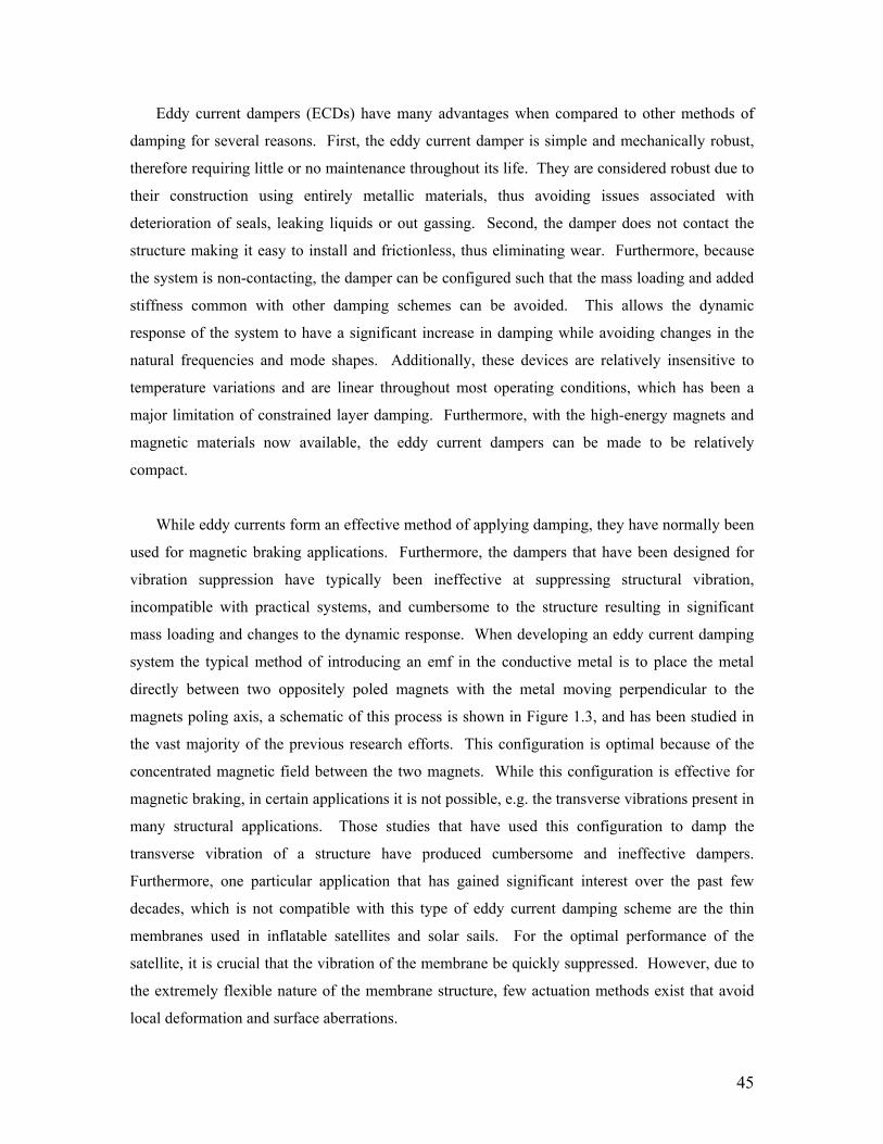
45

Eddy current dampers (ECDs) have many advantages when compared to other methods of

damping for several reasons. First, the eddy current damper is simple and mechanically robust,

therefore requiring little or no maintenance throughout its life. They are considered robust due to

their construction using entirely metallic materials, thus avoiding issues associated with

deterioration of seals, leaking liquids or out gassing. Second, the damper does not contact the

structure making it easy to install and frictionless, thus eliminating wear. Furthermore, because

the system is non-contacting, the damper can be configured such that the mass loading and added

stiffness common with other damping schemes can be avoided. This allows the dynamic

response of the system to have a significant increase in damping while avoiding changes in the

natural frequencies and mode shapes. Additionally, these devices are relatively insensitive to

temperature variations and are linear throughout most operating conditions, which has been a

major limitation of constrained layer damping. Furthermore, with the high-energy magnets and

magnetic materials now available, the eddy current dampers can be made to be relatively

compact.

While eddy currents form an effective method of applying damping, they have normally been

used for magnetic braking applications. Furthermore, the dampers that have been designed for

vibration suppression have typically been ineffective at suppressing structural vibration,

incompatible with practical systems, and cumbersome to the structure resulting in significant

mass loading and changes to the dynamic response. When developing an eddy current damping

system the typical method of introducing an emf in the conductive metal is to place the metal

directly between two oppositely poled magnets with the metal moving perpendicular to the

magnets poling axis, a schematic of this process is shown in Figure 1.3, and has been studied in

the vast majority of the previous research efforts. This configuration is optimal because of the

concentrated magnetic field between the two magnets. While this configuration is effective for

magnetic braking, in certain applications it is not possible, e.g. the transverse vibrations present in

many structural applications. Those studies that have used this configuration to damp the

transverse vibration of a structure have produced cumbersome and ineffective dampers.

Furthermore, one particular application that has gained significant interest over the past few

decades, which is not compatible with this type of eddy current damping scheme are the thin

membranes used in inflatable satellites and solar sails. For the optimal performance of the

satellite, it is crucial that the vibration of the membrane be quickly suppressed. However, due to

the extremely flexible nature of the membrane structure, few actuation methods exist that avoid

local deformation and surface aberrations.

46

To overcome the limitations associated with the presently available eddy current dampers this

dissertation will develop several new damping mechanisms that can be applied to a structure in a

non contact way to provide significant damping. This chapter will develop the theoretical model

of a novel passive eddy current damper. However, while the chapter focuses on this passive

damping concept the theoretical models developed in this chapter will later be modified to predict

the damping capabilities of a semi-active damper and an active damper in subsequent chapters.

Furthermore, this chapter will only derive the models necessary to predict the effect of the

damper on the applied structure and the validation of these models will be provided in chapter 3.

2.2 Theoretical Model of the Passive Eddy Current Damper

2.2.1 Passive Eddy Current Damper Configuration

The passive eddy current damping concept that will be developed and modeling in this

chapter consists of a permanent magnet that is both fixed in positions and strength and located a

small distance, typically between 1 and 10mm from the beam. The motion of the beam is in the

poling direction of the magnetic as shown in Figure 2.1. Due to the permanent magnet a

magnetic field is generated and due to the motion of the beam in this field, the conductor

experiences a time varying magnetic flux inducing eddy currents in the conducing sheet that has

been attached to the beam. Figure 2.2 shows the conducting sheet of thickness δ and conductivity

σ moving with velocity v in the gap lg between the circular magnet and the conductor. Figure 2.2,

also shows that the eddy currents circulate on the conducting sheet in the x-y plane, causing a

magnetic field to be generated that will interact with the applied field.

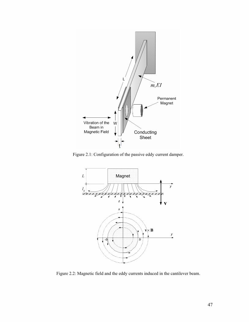
47

t

Figure 2.1: Configuration of the passive eddy current damper.

Magnet

x

y

z

y

v

×v B

gl

L

b-b

Figure 2.2: Magnetic field and the eddy currents induced in the cantilever beam.

48

2.2.2 Eddy Current Damping Force

The symmetry of the circular permanent magnet allows the surface charges to be ignored and

thus the eddy current density J induced in the conductive sheet due to the applied magnetic flux

B, can be written as

( )BvJ ×= σ (2.1)

where v is the velocity, σ is the conductivity, and the term ×v B is an electromotive force

driving the eddy currents J . The velocity and magnetic flux can be written as follows

kjiv zv++= 00 (2.2)

kjiB zyx BBB ++= (2.3)

where the velocity is only in the z-direction. Substitution of equations (2.2) and (2.3) into

equation (2.1) allows the eddy current density to be defined by

( ) ( )jiBvJ xyz BBv +−=×= σσ (2.4)

The above equation shows that the magnetic flux in the z-direction has no effect on the induced

eddy currents and that the induced currents are solely dependent on the x- and y-components of

the magnetic flux or the flux tangential to the face of the conducting sheet. This is an important

concept to note because it is opposite of the way that eddy currents are generated in magnetic

braking applications. Therefore, the typical design of eddy current dampers must be reconsidered

when developing the type of dampers analyzed in this dissertation.

Since the magnetization inside the magnet is constant, there is no equivalent volume current

density and the equivalent magnetization can be analyzed as a surface current density on the side

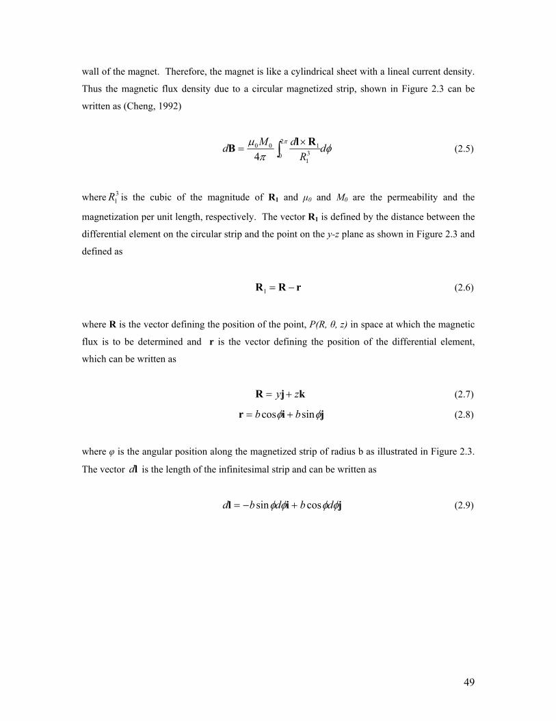
49

wall of the magnet. Therefore, the magnet is like a cylindrical sheet with a lineal current density.

Thus the magnetic flux density due to a circular magnetized strip, shown in Figure 2.3 can be

written as (Cheng, 1992)

φπ

µ πd

RdMd ∫×

=2

0 31

100

4RlB (2.5)

where 31R is the cubic of the magnitude of R1 and µ0 and M0 are the permeability and the

magnetization per unit length, respectively. The vector R1 is defined by the distance between the

differential element on the circular strip and the point on the y-z plane as shown in Figure 2.3 and

defined as

rRR −=1 (2.6)

where R is the vector defining the position of the point, P(R, θ, z) in space at which the magnetic

flux is to be determined and r is the vector defining the position of the differential element,

which can be written as

kjR zy += (2.7)

jir φφ sincos bb += (2.8)

where φ is the angular position along the magnetized strip of radius b as illustrated in Figure 2.3.

The vector dl is the length of the infinitesimal strip and can be written as

jil φφφφ dbdbd cossin +−= (2.9)

50

φ

R

1R

rθ

( ), ,P R zθ

y

z

x

dlb

b

Figure 2.3: Schematic of the Circular magnetized strip depicting the variable used in the analysis.

Substitution of equations (2.6) and (2.9) into equation (2.5) allows the magnetic flux density

due to the circular magnetized strip to be written as

( )( )zybIbzMd

ybzyb

bzMdBy ,,4sin2

sin4 1

002

0 23222

00

πµφ

φ

φπ

µ π=

−++= ∫ (2.10)

( )( )zybIbMd

ybzyb

ybbMdBz ,,4sin2

sin4 2

002

0 23222

00

πµφ

φ

φπ

µ π=

−++

−= ∫ (2.11)

where 1I and 2I include elliptic integrals that do not have a closed form solution and are shown

in Appendix A. To obtain the magnetic flux density due to the entire permanent magnet the flux

form the strip must be integrated over the length of the magnet. Hence, the magnetic flux density

in the radial or y-direction and the poling or z-direction due to the circular cylindrical magnet of

length L are written by

( ) ( ) ( )∫− ′′−′−=0

100 ,,

4,

Ly zdzzybIzzbMzyBπ

µ (2.12)

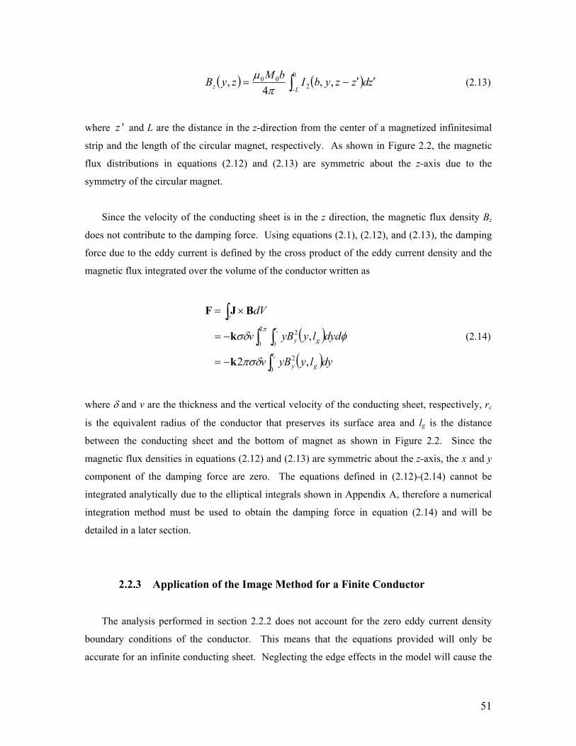
51

( ) ( )∫− ′′−=0

200 ,,

4,

Lz zdzzybIbMzyBπ

µ (2.13)

where 'z and L are the distance in the z-direction from the center of a magnetized infinitesimal

strip and the length of the circular magnet, respectively. As shown in Figure 2.2, the magnetic

flux distributions in equations (2.12) and (2.13) are symmetric about the z-axis due to the

symmetry of the circular magnet.

Since the velocity of the conducting sheet is in the z direction, the magnetic flux density Bz

does not contribute to the damping force. Using equations (2.1), (2.12), and (2.13), the damping

force due to the eddy current is defined by the cross product of the eddy current density and the

magnetic flux integrated over the volume of the conductor written as

( )( )∫

∫ ∫∫

−=

−=

×=

c

c

r

gy

g

r

y

V

dylyyBv

dydlyyBv

dV

0

2

2

0 0

2

,2

,

πσδ

φσδπ

k

k

BJF

(2.14)

where δ and v are the thickness and the vertical velocity of the conducting sheet, respectively, rc

is the equivalent radius of the conductor that preserves its surface area and lg is the distance

between the conducting sheet and the bottom of magnet as shown in Figure 2.2. Since the

magnetic flux densities in equations (2.12) and (2.13) are symmetric about the z-axis, the x and y

component of the damping force are zero. The equations defined in (2.12)-(2.14) cannot be

integrated analytically due to the elliptical integrals shown in Appendix A, therefore a numerical

integration method must be used to obtain the damping force in equation (2.14) and will be

detailed in a later section.

2.2.3 Application of the Image Method for a Finite Conductor

The analysis performed in section 2.2.2 does not account for the zero eddy current density

boundary conditions of the conductor. This means that the equations provided will only be

accurate for an infinite conducting sheet. Neglecting the edge effects in the model will cause the

52

predicted damping to be greater than actually present, because the eddy current density is not

required to be zero at the edges. The result of this is that the integration over the volume of the

conductor performed in equation (2.14) will result in an increased damping force even if the

integration is not performed over an infinite domain. In order to account for the edge effects, the

image method (Lee and Park, 2002) can be used to satisfy the boundary condition of zero eddy

current density at the conducting plate’s boundaries. The technique of using the image method

consists of calculating the eddy current density then creating a mirror image of the calculated

density that is rotated about the edge of the conductor. Following this, the imaginary density is

subtracted from the eddy current density, thus enforcing a zero density condition at the edge of

the conductor. A schematic showing how the image method is used can be seen in Figure 2.4.

Figure 2.4: Schematic demonstrating the effect of the imaginary eddy currents.

Mathematically this process is as follows: the incorporation of the imaginary eddy current

density, allows the net eddy current in the radial direction J ′ , to be written as

( ))2()1(yy JJ −=′J (2.15)

where the subscript y indicates the radial direction and the imaginary eddy current density ( )2yJ is

written as

)2()( )1()2( yAJyJ yy −= (2.16)

53

where ( )1yJ is the predicted eddy current density from equation 2.4 and the dimension A

corresponds to half the length of the conducting plate as shown in Figure 2.5. Only one

imaginary eddy current is needed because the conductor is modeled as a circular plate with the

same area as the original conductor as shown in Figure 2.5. This assumption is made to simplify

the integration of equations (2.12)-(2.14). Substituting equations (2.15) and (2.16) into equation

(2.14), the damping force accounting for the imaginary eddy currents is defined as

( ) ( )

( ) ( ) ⎥⎦⎤

⎢⎣⎡ −−−=

⎥⎦⎤

⎢⎣⎡ −−−=

×′=

∫∫

∫ ∫∫ ∫

∫

cc

cc

r

gy

r

gy

g

r

yg

r

y

V

dylyAyBdylyyBv

dydlyAyBdydlyyBv

dV

0

2

0

2

2

0 0

22

0 0

2

,2,2

,2,

πσδ

φφσδππ

k

k

BJF

(2.17)

As before, the integration of equation (2.17) cannot be analytically performed and must therefore

be determined using a numerical technique. From equation (2.17) it is apparent that the eddy

current force is a viscous force because the velocity of the beam, v, is directly proportional to the

magnitude of the force. The resulting value of this force can be coupled into the equations of

motion for the system that it will be interacting with.

In this dissertation the ability of the passive damper to suppress the vibration of a cantilever

beam and a thin membrane subjected to an axial load will be studied. This will allows

experiments to be precisely performed such that the accuracy of that the theoretical model can be

identified without concern in error from experiments of more complex structural models. In the

following section the mathematical model of a beam with the eddy current damping force

incorporated into its dynamic response will be developed. Subsequent to this, section 2.2.5 will

derive the equations of motion for a thin membrane under axial load with the eddy current

damper.

54

Figure 2.5: Schematic showing the variables associated with the conducting plate.

2.2.4 Modeling of Beam with Eddy Current Damping Force

The dynamic response of the beam can be formulated using the assumed modes method

applied to an Euler-Bernoulli beam. This method assumes that the response can be modeled as a

summation of trial functions that satisfy the boundary conditions of the system and a temporal

coordinate as

( ) ( ) ( ) ( ) ( )trxtrxtxuN

iii φφ == ∑

=1

, (2.18)

where )(xiφ is the assumed mode shapes of the structure that can be set to satisfy any

combination of boundary conditions, r(t) is the temporal coordinate of the displacement, and N is

the number of modes to be included in the analysis. The kinetic energy T, potential energy V,

non-conservative forces D, and external forces Q for the beam are defined by

( )

∫ ⎥⎦⎤

⎢⎣⎡

∂∂

=L

dxt

txuT0

2,21 ρ (2.19)

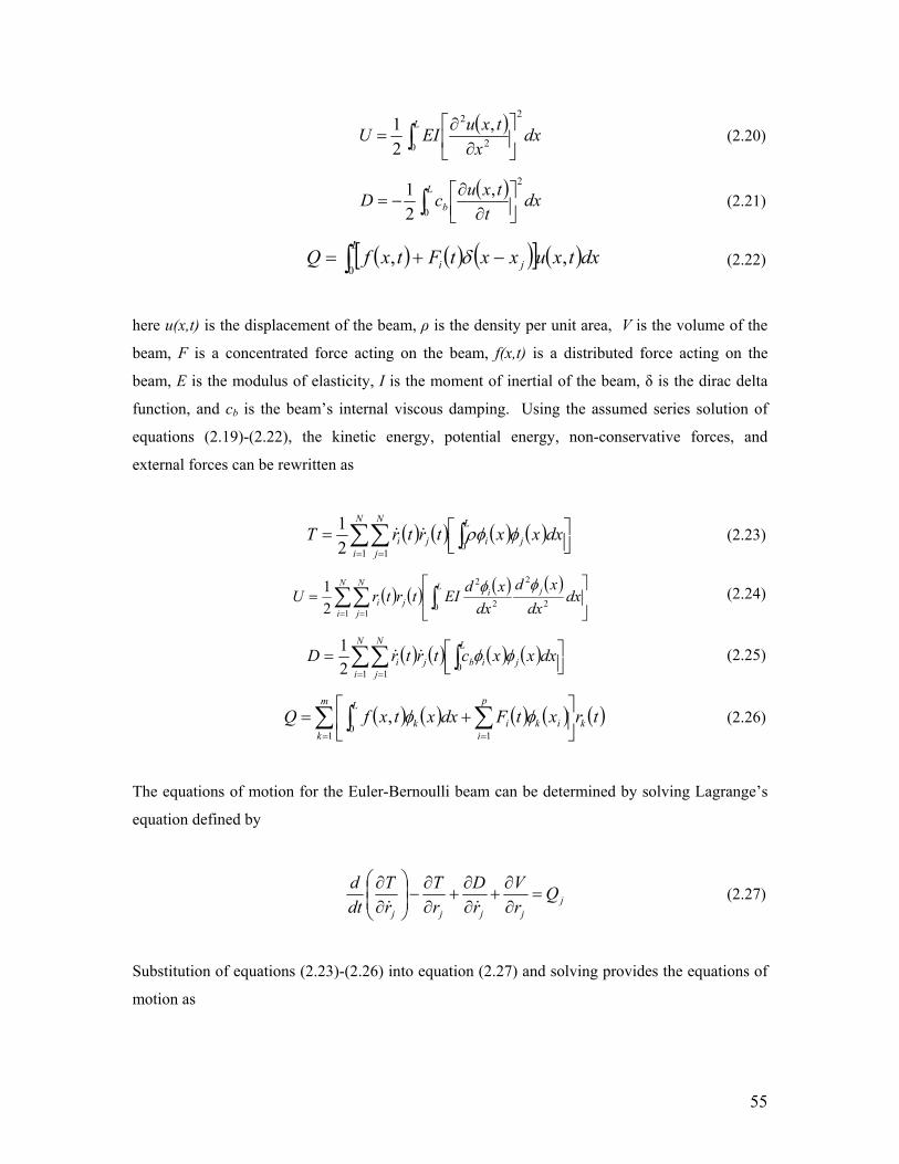
55

( )∫ ⎥

⎦

⎤⎢⎣

⎡∂

∂=

Ldx

xtxuEIU

0

2

2

2 ,21

(2.20)

( )∫ ⎥⎦

⎤⎢⎣⎡

∂∂

−=L

b dxt

txucD0

2,21

(2.21)

( ) ( ) ( )[ ] ( )∫ −+=L

ji dxtxuxxtFtxfQ0

,, δ (2.22)

here u(x,t) is the displacement of the beam, ρ is the density per unit area, V is the volume of the

beam, F is a concentrated force acting on the beam, f(x,t) is a distributed force acting on the

beam, E is the modulus of elasticity, I is the moment of inertial of the beam, δ is the dirac delta

function, and cb is the beam’s internal viscous damping. Using the assumed series solution of

equations (2.19)-(2.22), the kinetic energy, potential energy, non-conservative forces, and

external forces can be rewritten as

( ) ( ) ( ) ( ) ⎥⎦⎤

⎢⎣⎡= ∫∑∑

= =

L

ji

N

i

N

jji dxxxtrtrT

01 12

1 φρφ (2.23)

( ) ( ) ( ) ( )⎥⎦

⎤⎢⎣

⎡= ∫∑∑

= =

L jiN

i

N

jji dx

dxxd

dxxdEItrtrU

0 2

2

2

2

1 121 φφ (2.24)

( ) ( ) ( ) ( ) ⎥⎦⎤

⎢⎣⎡= ∫∑∑

= =

L

jib

N

i

N

jji dxxxctrtrD

01 12

1 φφ (2.25)

( ) ( ) ( ) ( ) ( )∑ ∫ ∑= =

⎥⎦

⎤⎢⎣

⎡+=

m

kk

L p

iikik trxtFdxxtxfQ

10

1

, φφ (2.26)

The equations of motion for the Euler-Bernoulli beam can be determined by solving Lagrange’s

equation defined by

jjjjj

QrV

rD

rT

rT

dtd

=∂∂

+∂∂

+∂∂

−⎟⎟⎠

⎞⎜⎜⎝

⎛

∂∂

(2.27)

Substitution of equations (2.23)-(2.26) into equation (2.27) and solving provides the equations of

motion as

56

( ) ( ) ( ) ( ) ( ) ( ) ( )∫ ∑=

+=++L p

iii xtFdxxtxftrtrtr

01

, φφKCM (2.28)

where the mass matrix M, damping matrix C, and the stiffness matrix K are determined by

substitution of the beam’s properties into the following equations

( ) ( )∫==L T

ij dxxxm0

φφρM (2.29)

( ) ( )∫==L

bT

ij dxxcxc0

φφC (2.30)

( ) ( )∫ ′′′′==L T

ij dxxxEIk0

φφK

(2.31)

The damping force generated by the eddy current damper is incorporated into the response of the

system as a concentrated force term that is dependent on the velocity between the magnet and the

beam defined by

( ) ( ) ( ) ( )trxcxtF eeφφ =11 (2.32)

where ( )exφ is the magnitude of the mode shape at the location of the eddy current damper, ce is

the eddy current damping force determined by dividing the eddy current force in equation (2.17)

by the velocity, v, and ( )tr is the velocity of the beam. Substitution of equations (2.29)-(2.32)

into equation (2.28) defines the equation of motion of the beam including the passive eddy

current damper. The accuracy of the modeling techniques used here will be experimentally

verified in chapter 3.

2.2.5 Modeling of Slender Membrane under Axial Load with Eddy Current

Damping Force

Due to the non-contact nature of the eddy current damper it is particularly well suited for use

with extremely flexible structures that cannot be controlled with traditional actuators, such as the

ultra large membranes used in inflatable space structures. For the optimal performance of the

satellite, it is crucial that the vibration of the membrane be quickly suppressed. However, due to

57

the extremely flexible nature of the membrane structure, few actuation methods exist that avoid

local deformation and surface aberrations.

Eddy currents do have many properties that make them ideal for use with these structures

because they are non-contacting and thus avoid surface irregularities due to bonding. In addition,

they apply a distributed force therefore minimizing localized excitation. However, the use of

eddy current damping mechanisms with the extremely thin materials has not been shown to be

capable of generating sufficient forces to suppress the structures vibrations. The problem that a

thin conductor may not function well as an eddy current damper can be seen by examining

equation (2.17), which shows that the damping force is directly related to the thickness of the

conductive medium. Therefore, the theoretical model of the eddy current damping system when

applied to a thin membrane will be developed to identify the compatibility of these thin

membranes and eddy current dampers.

The membrane used for this study was chosen to resemble a beam rather than a 2-

dimensional membrane, thus allowing dynamic testing to be performed in the available vacuum

chamber. A schematic of the layout of the membrane and magnetic are shown in Figure 2.6.

Because the Membrane is extremely flexible in nature, both excitation and sensing methods are

very limited. By using a slender membrane the ability to experimentally identify bending modes

and correlate them with the model is greatly simplified. Furthermore, the question is not whether

the passive eddy current damping techniques will work on a 2-dimensional membrane but rather

if they will generate sufficient damping forces on a very thin structure. Additionally, because this

system is passive, it does not have stability issues that would make the damper effective for use

with a slender membrane but ineffective with a 2-dimensional membrane, thus if it can

effectively add damping to a slender membrane then it will also add damping to a 2-diminsional

structure.

58

Figure 2.6: Schematic of the configuration of the membrane and permanent magnet.

The membrane itself is typically not conductive and therefore must have some type of

conductive coating applied to it. In space applications, the membrane would be constructed with

a conductive layer on one side, however, this type of material was not available. Because the

commercially available membranes were not conductive, a conductive copper material was

applied to the membrane, the details of which will be supplied in chapter 3. While the membrane

used in this research is a one dimension structure and could be modeled as a string, the copper

conductor bonded to the membrane material is not void of stiffness. Therefore a beam model

must be used to allow the stiffness of the copper patch to be included in the model. The structure

can be modeled as an Euler-Bernoulli beam subjected to an axial load. The equation of motion

for a beam under an axial load was formulated by Shaker (1975) as

( )( )

( ) ( )( )

( ) 0,,,2

2

2

2

4

4

=∂

∂+

∂∂

+∂

∂t

txwxEIx

xtxw

xEIP

xtxw ρ

(2.34)

where w(x,t) is the transverse deflection of the beam, P is the axial load, ρ(x) is the mass per unit

length, and EI(x) is the beading stiffness along the x-direction of the membrane and copper patch.

From the equation of motion, the kinetic energy and potential energy can be written as

( ) ( ) dxt

txwxTL

2

0

,21∫ ⎥⎦

⎤⎢⎣⎡

∂∂

= ρ (2.35)

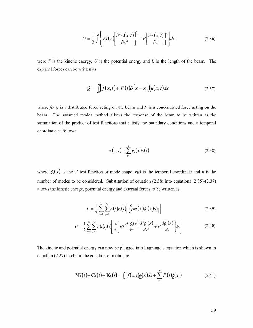
59

( ) ( ) ( ) dxx

txwPx

txwxEIUL

∫⎪⎭

⎪⎬⎫

⎪⎩

⎪⎨⎧

⎥⎦⎤

⎢⎣⎡

∂∂

+⎥⎦

⎤⎢⎣

⎡∂

∂=

0

22

2

2 ,,21

(2.36)

were T is the kinetic energy, U is the potential energy and L is the length of the beam. The

external forces can be written as

( ) ( ) ( )[ ] ( )∫ −+=L

ji dxtxuxxtFtxfQ0

,, δ (2.37)

where f(x,t) is a distributed force acting on the beam and F is a concentrated force acting on the

beam. The assumed modes method allows the response of the beam to be written as the

summation of the product of test functions that satisfy the boundary conditions and a temporal

coordinate as follows

( ) ( ) ( )∑=

=n

iii trxtxw

1

, φ (2.38)

where ( )xiφ is the ith test function or mode shape, r(t) is the temporal coordinate and n is the

number of modes to be considered. Substitution of equation (2.38) into equations (2.35)-(2.37)

allows the kinetic energy, potential energy and external forces to be written as

( ) ( ) ( ) ( ) ⎥⎦⎤

⎢⎣⎡= ∫∑∑

= =

L

ji

N

i

N

jji dxxxtrtrT

01 12

1 φρφ (2.39)

( ) ( ) ( ) ( ) ( )⎥⎥⎦

⎤

⎢⎢⎣

⎡⎟⎟⎠

⎞⎜⎜⎝

⎛+= ∫∑∑

= =

L jjiN

i

N

jji dx

dxxd

Pdx

xddx

xdEItrtrU0 2

2

2

2

1 121 φφφ (2.40)

The kinetic and potential energy can now be plugged into Lagrange’s equation which is shown in

equation (2.27) to obtain the equation of motion as

( ) ( ) ( ) ( ) ( ) ( ) ( )∫ ∑=

+=++L p

iii xtFdxxtxftrtrtr

01

, φφKCM (2.41)

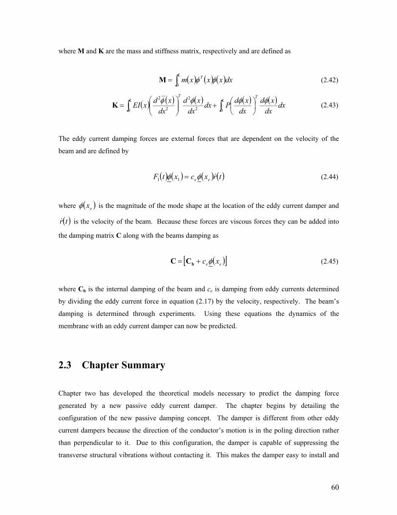
60

where M and K are the mass and stiffness matrix, respectively and are defined as

( ) ( ) ( )dxxxxmL T φφ∫= 0

M (2.42)

( ) ( ) ( ) ( ) ( )∫∫ ⎟

⎠⎞

⎜⎝⎛+⎟⎟

⎠

⎞⎜⎜⎝

⎛=

LT

LT

dxdx

xddx

xdPdxdx

xddx

xdxEI00 2

2

2

2 φφφφK (2.43)

The eddy current damping forces are external forces that are dependent on the velocity of the

beam and are defined by

( ) ( ) ( ) ( )trxcxtF eeφφ =11 (2.44)

where ( )exφ is the magnitude of the mode shape at the location of the eddy current damper and

( )tr is the velocity of the beam. Because these forces are viscous forces they can be added into

the damping matrix C along with the beams damping as

( )[ ]ee xc φ+= bCC (2.45)

where Cb is the internal damping of the beam and ce is damping from eddy currents determined

by dividing the eddy current force in equation (2.17) by the velocity, respectively. The beam’s

damping is determined through experiments. Using these equations the dynamics of the

membrane with an eddy current damper can now be predicted.

2.3 Chapter Summary

Chapter two has developed the theoretical models necessary to predict the damping force

generated by a new passive eddy current damper. The chapter begins by detailing the

configuration of the new passive damping concept. The damper is different from other eddy

current dampers because the direction of the conductor’s motion is in the poling direction rather

than perpendicular to it. Due to this configuration, the damper is capable of suppressing the

transverse structural vibrations without contacting it. This makes the damper easy to install and

61

allows significant damping to be added while allowing the other properties and dynamics of the

structure to be unaffected by its addition to the system. Furthermore, because the damped is of

passive nature it is robust to parameter changes and requires no additional energy. However, this

configuration of the damper does require some type of secondary structure to support the magnet,

which may be a draw back in certain structures.

While the system provides advantages over other damping techniques, the performance of the

new system is significantly different from those that have been traditionally used. For this reason

the theoretical model of the damper had not been previously developed. Therefore, chapter 2 has

deriving the equations required to determine the eddy current damping force generated by a

cylindrical permanent magnet in close proximity to a vibrating structure. This derivation requires

that the magnetic flux of the magnetic be identified such that the eddy current density can be

determined. Typical eddy current dampers use two magnets positioned such that opposite poles

are facing each other with a small gap between them. This configuration allows the magnetic

flux between the magnets to be assumed to be constant. However, because the damper that has

been developed in this chapter is not configured in this way, the entire magnetic flux around the

magnet must be determined. The solution for the magnetic flux has been identified; however the

necessary integration cannot be analytically solved, requiring a numerical technique to be used.

Following the identification of the magnetic flux from the magnet the eddy current density and

eddy current damping force can be found. It was shown that unlike traditional eddy current

dampers the radial magnetic flux is responsible for the creation of eddy currents rather than the

magnetic flux in the poling direction. Additionally, the eddy current damping force is dependent

on the velocity of the conductor in the magnetic field causing the system to function as a viscous

damper.

Once the eddy current damping force had been identified it could be incorporated into the

dynamic equations of the structure it will be integrated into. In this dissertation, the passive

damper will be used to suppress the vibration of a beam and a thin membrane. A thin membrane

is investigated because the eddy current damping force is dependent on the thickness of the

conductor and therefore may not be able to generate sufficient force to suppress the vibration of

an extremely thin structure. Therefore, a theoretical derivation of the equation of motion for

these two systems was performed. Because the eddy current force is a viscous term it can be

easily included in the damping terms of the equation of motion. In the chapter 3 an experimental

validation of the equations developed in this chapter will be performed. This validation will show

62

the accuracy of the equations derived here and demonstrate the effectiveness of this damping

mechanism. Additionally, results of the numerical analysis of the eddy current damping force

and magnetic flux will be provided.

63

Chapter 3

Experimental Verification of Passive

Eddy Current Damper Models

3.1 Chapter Introduction

Past eddy current dampers that were designed to suppress transverse vibrations have typically

been incompatible with practical systems, ineffective at suppressing structural vibration, and

cumbersome to the structure resulting in significant mass loading and changes to the dynamic

response. Zheng et al. (2003) developed a damping system that functioned by placing a magnetic

near the root of a beam, and using a coil mounted at the clamped boundary condition to generate

a controlled magnetic force to suppress the vibration. The system was shown to provide

additional damping; however this added damping was small and the number of applicable

structures was significantly limited. A study performed by Kwak et al. (2003), developed an

eddy current damper that consisted of two permanent magnets attached to a cantilever beam with

a flexible linkage. The linkage allowed the magnets to move past a conductive plate rigidly fixed

at the end of the beam. Through a theoretical analysis and experiments, the damper was shown to

apply significant damping to the beam. On the other hand the system was only compatible with a

cantilever type structure and substantially changed the dynamics of the beam. The studies

discussed above are only two of the many eddy current damping systems developed to suppress

structural vibrations (see chapter 1 for details); however, both show the common limitations faced

by most all currently available eddy current dampers.

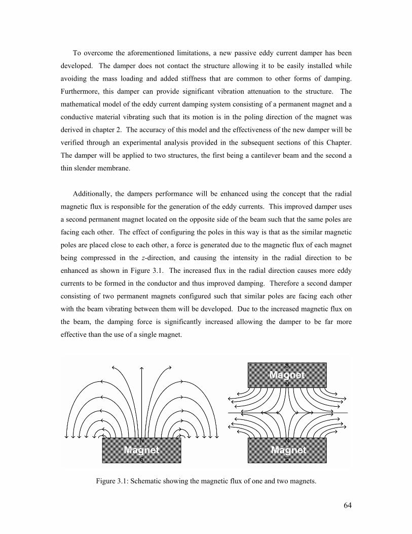
64

To overcome the aforementioned limitations, a new passive eddy current damper has been

developed. The damper does not contact the structure allowing it to be easily installed while

avoiding the mass loading and added stiffness that are common to other forms of damping.

Furthermore, this damper can provide significant vibration attenuation to the structure. The

mathematical model of the eddy current damping system consisting of a permanent magnet and a

conductive material vibrating such that its motion is in the poling direction of the magnet was

derived in chapter 2. The accuracy of this model and the effectiveness of the new damper will be

verified through an experimental analysis provided in the subsequent sections of this Chapter.

The damper will be applied to two structures, the first being a cantilever beam and the second a

thin slender membrane.

Additionally, the dampers performance will be enhanced using the concept that the radial

magnetic flux is responsible for the generation of the eddy currents. This improved damper uses

a second permanent magnet located on the opposite side of the beam such that the same poles are

facing each other. The effect of configuring the poles in this way is that as the similar magnetic

poles are placed close to each other, a force is generated due to the magnetic flux of each magnet

being compressed in the z-direction, and causing the intensity in the radial direction to be

enhanced as shown in Figure 3.1. The increased flux in the radial direction causes more eddy

currents to be formed in the conductor and thus improved damping. Therefore a second damper

consisting of two permanent magnets configured such that similar poles are facing each other

with the beam vibrating between them will be developed. Due to the increased magnetic flux on

the beam, the damping force is significantly increased allowing the damper to be far more

effective than the use of a single magnet.

Figure 3.1: Schematic showing the magnetic flux of one and two magnets.

65

3.2 Experimental Testing and Results of the Passive Eddy

Current Damper Concept

The passive eddy current damper consists of a single permanent magnet fixed a small distance

from a vibrating beam with a conductive patch bonded to its surface. The beam vibrates in the

magnetic field such that its motion is in line with the poling direction of the magnet causing the

radial magnetic flux to induce an electromotive force (emf). This emf allows the eddy currents to

be continuously generated and subsequently dissipated by the internal resistance of the

conductive material. The dissipation of the eddy currents causes a removal of energy form the

system and a damping force. In section 3.2 of this chapter, the passive eddy current damper

utilizing a single permanent magnet will be experimentally tested to both show it’s effectiveness

as a vibration damping mechanism, and to demonstrate the accuracy of the model developed in

Chapter 2.

3.2.1 Passive Eddy Current Damper Experimental Setup

In order to validate the accuracy of the model, experiments were performed on an aluminum

beam with dimensions shown in Figure 3.2. For all tests performed on the cantilever beam a

neodymium-iron-boron permanent magnet with radius and length of 6.35mm and 12.7mm,

respectively, was used. The other physical properties of the beam, conductor, and magnet are

listed in Table 3.1. When performing the validation of the model, it was necessary to include the

effect of the eddy currents generated in the aluminum beam, because of its high conductivity.

Figure 3.2: Schematic showing the dimensions of the beam.

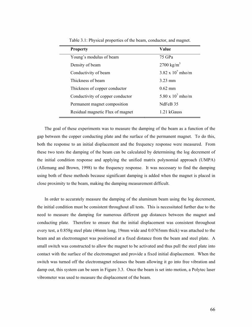
66

Table 3.1: Physical properties of the beam, conductor, and magnet.

Property Value

Young’s modulus of beam 75 GPa

Density of beam 2700 kg/m3

Conductivity of beam 3.82 x 107 mho/m

Thickness of beam 3.23 mm

Thickness of copper conductor 0.62 mm

Conductivity of copper conductor 5.80 x 107 mho/m

Permanent magnet composition NdFeB 35

Residual magnetic Flux of magnet 1.21 kGauss

The goal of these experiments was to measure the damping of the beam as a function of the

gap between the copper conducting plate and the surface of the permanent magnet. To do this,

both the response to an initial displacement and the frequency response were measured. From

these two tests the damping of the beam can be calculated by determining the log decrement of

the initial condition response and applying the unified matrix polynomial approach (UMPA)

(Allemang and Brown, 1998) to the frequency response. It was necessary to find the damping

using both of these methods because significant damping is added when the magnet is placed in

close proximity to the beam, making the damping measurement difficult.

In order to accurately measure the damping of the aluminum beam using the log decrement,

the initial condition must be consistent throughout all tests. This is necessitated further due to the

need to measure the damping for numerous different gap distances between the magnet and

conducting plate. Therefore to ensure that the initial displacement was consistent throughout

every test, a 0.858g steel plate (46mm long, 19mm wide and 0.0765mm thick) was attached to the

beam and an electromagnet was positioned at a fixed distance from the beam and steel plate. A

small switch was constructed to allow the magnet to be activated and thus pull the steel plate into

contact with the surface of the electromagnet and provide a fixed initial displacement. When the

switch was turned off the electromagnet releases the beam allowing it go into free vibration and

damp out, this system can be seen in Figure 3.3. Once the beam is set into motion, a Polytec laser

vibrometer was used to measure the displacement of the beam.

67

Figure 3.3: Experimental setup of the aluminum beam and eddy current damper.

To measure the frequency response of the aluminum beam, a piezoelectric patch was attached

at the root of the beam as an excitation source, while the beam’s response was measured using a

Polytec laser vibrometer. With the two excitation systems developed (initial condition and

piezoelectric induced disturbance), the next step was to construct an accurate method of

positioning the permanent magnet a fixed distance from the conducting plate. To allow the

position of the magnet to be accurately varied, it was bonded to a wooden block that was fixed to

a lead screw, as sown in Figure 3.3. A wooden block was used such that the magnetic field was

not distorted due to high permeability materials in close proximity to the magnet. The

combination of a lead screw for positioning, an electromagnet for consistent initial displacement,

a permanently bonded piezoelectric patch and a non-contact sensing system, (laser vibrometer)

allowed every test to be precisely repeated.

.

Electromagnet

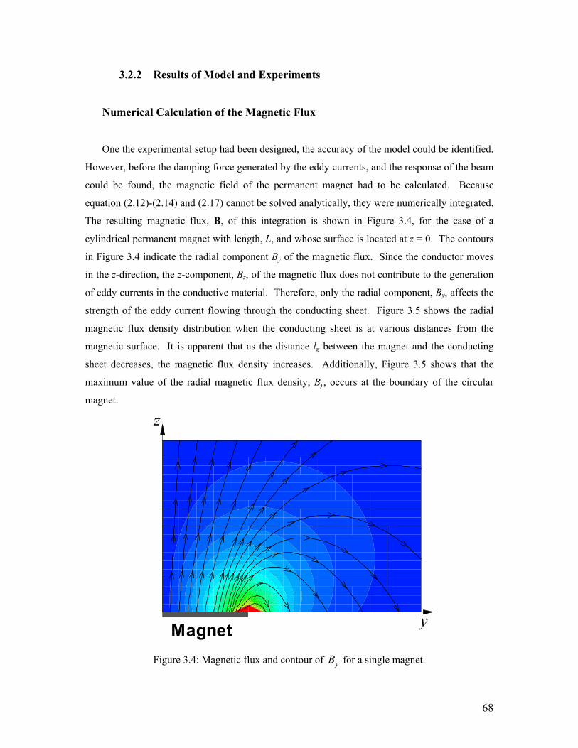
68

3.2.2 Results of Model and Experiments

Numerical Calculation of the Magnetic Flux

One the experimental setup had been designed, the accuracy of the model could be identified.

However, before the damping force generated by the eddy currents, and the response of the beam

could be found, the magnetic field of the permanent magnet had to be calculated. Because

equation (2.12)-(2.14) and (2.17) cannot be solved analytically, they were numerically integrated.

The resulting magnetic flux, B, of this integration is shown in Figure 3.4, for the case of a

cylindrical permanent magnet with length, L, and whose surface is located at z = 0. The contours

in Figure 3.4 indicate the radial component By of the magnetic flux. Since the conductor moves

in the z-direction, the z-component, Bz, of the magnetic flux does not contribute to the generation

of eddy currents in the conductive material. Therefore, only the radial component, By, affects the

strength of the eddy current flowing through the conducting sheet. Figure 3.5 shows the radial

magnetic flux density distribution when the conducting sheet is at various distances from the

magnetic surface. It is apparent that as the distance lg between the magnet and the conducting

sheet decreases, the magnetic flux density increases. Additionally, Figure 3.5 shows that the

maximum value of the radial magnetic flux density, By, occurs at the boundary of the circular

magnet.

Magnet y

z

Figure 3.4: Magnetic flux and contour of yB for a single magnet.

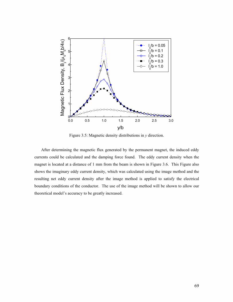
69

0.0 0.5 1.0 1.5 2.0 2.5 3.00

1

2

3

4

5

6

lg/b = 0.05 lg/b = 0.1 lg/b = 0.2 lg/b = 0.3 lg/b = 1.0

Mag

netic

Flu

x D

ensi

ty, B

y/(µ 0M

0b/4π)

y/b Figure 3.5: Magnetic density distributions in y direction.

After determining the magnetic flux generated by the permanent magnet, the induced eddy

currents could be calculated and the damping force found. The eddy current density when the

magnet is located at a distance of 1 mm from the beam is shown in Figure 3.6. This Figure also

shows the imaginary eddy current density, which was calculated using the image method and the

resulting net eddy current density after the image method is applied to satisfy the electrical

boundary conditions of the conductor. The use of the image method will be shown to allow our

theoretical model’s accuracy to be greatly increased.

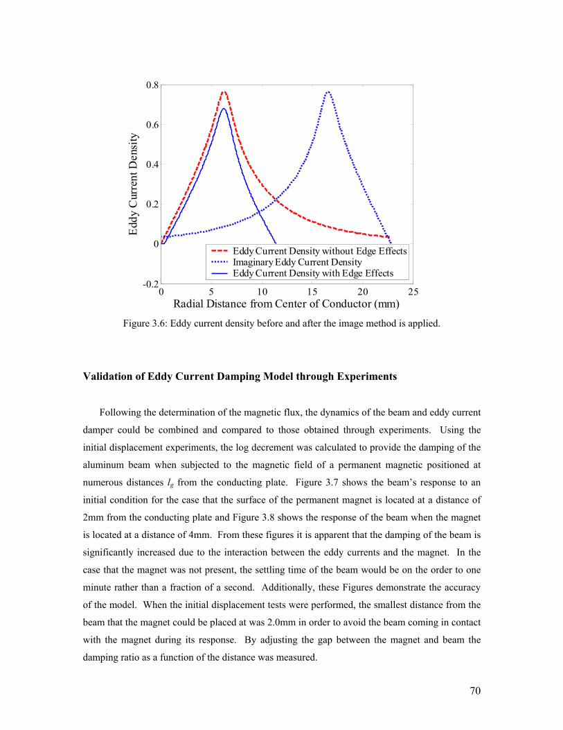
70

0 5 10 15 20 25-0.2

0

0.2

0.4

0.6

0.8

Radial Distance from Center of Conductor (mm)

Eddy

Cur

rent

Den

sity

Eddy Current Density without Edge EffectsImaginary Eddy Current DensityEddy Current Density with Edge Effects

Figure 3.6: Eddy current density before and after the image method is applied.

Validation of Eddy Current Damping Model through Experiments

Following the determination of the magnetic flux, the dynamics of the beam and eddy current

damper could be combined and compared to those obtained through experiments. Using the

initial displacement experiments, the log decrement was calculated to provide the damping of the

aluminum beam when subjected to the magnetic field of a permanent magnetic positioned at

numerous distances lg from the conducting plate. Figure 3.7 shows the beam’s response to an

initial condition for the case that the surface of the permanent magnet is located at a distance of

2mm from the conducting plate and Figure 3.8 shows the response of the beam when the magnet

is located at a distance of 4mm. From these figures it is apparent that the damping of the beam is

significantly increased due to the interaction between the eddy currents and the magnet. In the

case that the magnet was not present, the settling time of the beam would be on the order to one

minute rather than a fraction of a second. Additionally, these Figures demonstrate the accuracy

of the model. When the initial displacement tests were performed, the smallest distance from the

beam that the magnet could be placed at was 2.0mm in order to avoid the beam coming in contact

with the magnet during its response. By adjusting the gap between the magnet and beam the

damping ratio as a function of the distance was measured.

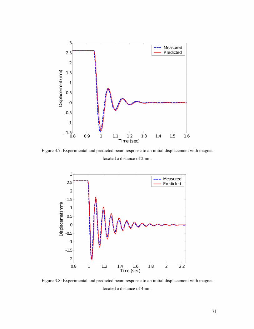
71

0.8 0.9 1 1.1 1.2 1.3 1.4 1.5 1.6-1.5

-1

-0.5

0

0.5

1

1.5

2

2.5

3

TIme (sec)

Dis

plac

emen

t (m

m)

MeasuredPredicted

Figure 3.7: Experimental and predicted beam response to an initial displacement with magnet

located a distance of 2mm.

0.8 1 1.2 1.4 1.6 1.8 2 2.2

-2

-1.5

-1

-0.5

0

0.5

1

1.5

2

2.5

3

Dis

plac

emet

(m

m)

MeasuredPredicted

Time (sec)

Figure 3.8: Experimental and predicted beam response to an initial displacement with magnet

located a distance of 4mm.

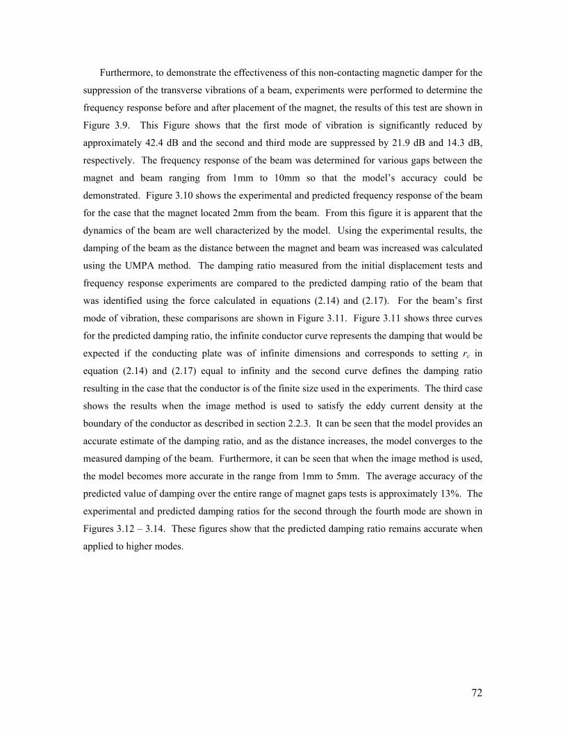
72

Furthermore, to demonstrate the effectiveness of this non-contacting magnetic damper for the

suppression of the transverse vibrations of a beam, experiments were performed to determine the

frequency response before and after placement of the magnet, the results of this test are shown in

Figure 3.9. This Figure shows that the first mode of vibration is significantly reduced by

approximately 42.4 dB and the second and third mode are suppressed by 21.9 dB and 14.3 dB,

respectively. The frequency response of the beam was determined for various gaps between the

magnet and beam ranging from 1mm to 10mm so that the model’s accuracy could be

demonstrated. Figure 3.10 shows the experimental and predicted frequency response of the beam

for the case that the magnet located 2mm from the beam. From this figure it is apparent that the

dynamics of the beam are well characterized by the model. Using the experimental results, the

damping of the beam as the distance between the magnet and beam was increased was calculated

using the UMPA method. The damping ratio measured from the initial displacement tests and

frequency response experiments are compared to the predicted damping ratio of the beam that

was identified using the force calculated in equations (2.14) and (2.17). For the beam’s first

mode of vibration, these comparisons are shown in Figure 3.11. Figure 3.11 shows three curves

for the predicted damping ratio, the infinite conductor curve represents the damping that would be

expected if the conducting plate was of infinite dimensions and corresponds to setting rc in

equation (2.14) and (2.17) equal to infinity and the second curve defines the damping ratio

resulting in the case that the conductor is of the finite size used in the experiments. The third case

shows the results when the image method is used to satisfy the eddy current density at the

boundary of the conductor as described in section 2.2.3. It can be seen that the model provides an

accurate estimate of the damping ratio, and as the distance increases, the model converges to the

measured damping of the beam. Furthermore, it can be seen that when the image method is used,

the model becomes more accurate in the range from 1mm to 5mm. The average accuracy of the

predicted value of damping over the entire range of magnet gaps tests is approximately 13%. The

experimental and predicted damping ratios for the second through the fourth mode are shown in

Figures 3.12 – 3.14. These figures show that the predicted damping ratio remains accurate when

applied to higher modes.

73

0 50 100 150 200 250-60

-50

-40

-30

-20

-10

0

10

20

Frequency (Hz)

Mag

nitu

de (d

B)

DampedUndamped

Figure 3.9: Experimentally measured damped and undamped frequency response of the beam.

0 50 100 150 200 250 300 350 400-60

-50

-40

-30

-20

-10

0

Frequncy (Hz)

Mag

nitu

de (dB

)

P redictedMeasured

Figure 3.10: Predicted and experimentally measured frequency response of the beam with the

magnet at a distance of 2mm.

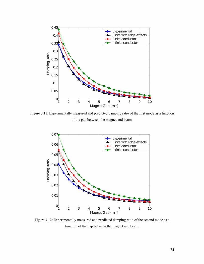
74

1 2 3 4 5 6 7 8 9 100

0.05

0.1

0.15

0.2

0.25

0.3

0.35

0.4

0.45

Magnet Gap (mm)

Dam

ping

Rat

io

ExperimentalFinite with edge effectsFinite conductorInfinite conductor

Figure 3.11: Experimentally measured and predicted damping ratio of the first mode as a function

of the gap between the magnet and beam.

1 2 3 4 5 6 7 8 9 100

0.01

0.02

0.03

0.04

0.05

0.06

0.07

Magnet Gap (mm)

Dam

ping

Rat

io

ExperimentalFinite with edge effectsFinite conductorInfinite conductor

Figure 3.12: Experimentally measured and predicted damping ratio of the second mode as a

function of the gap between the magnet and beam.

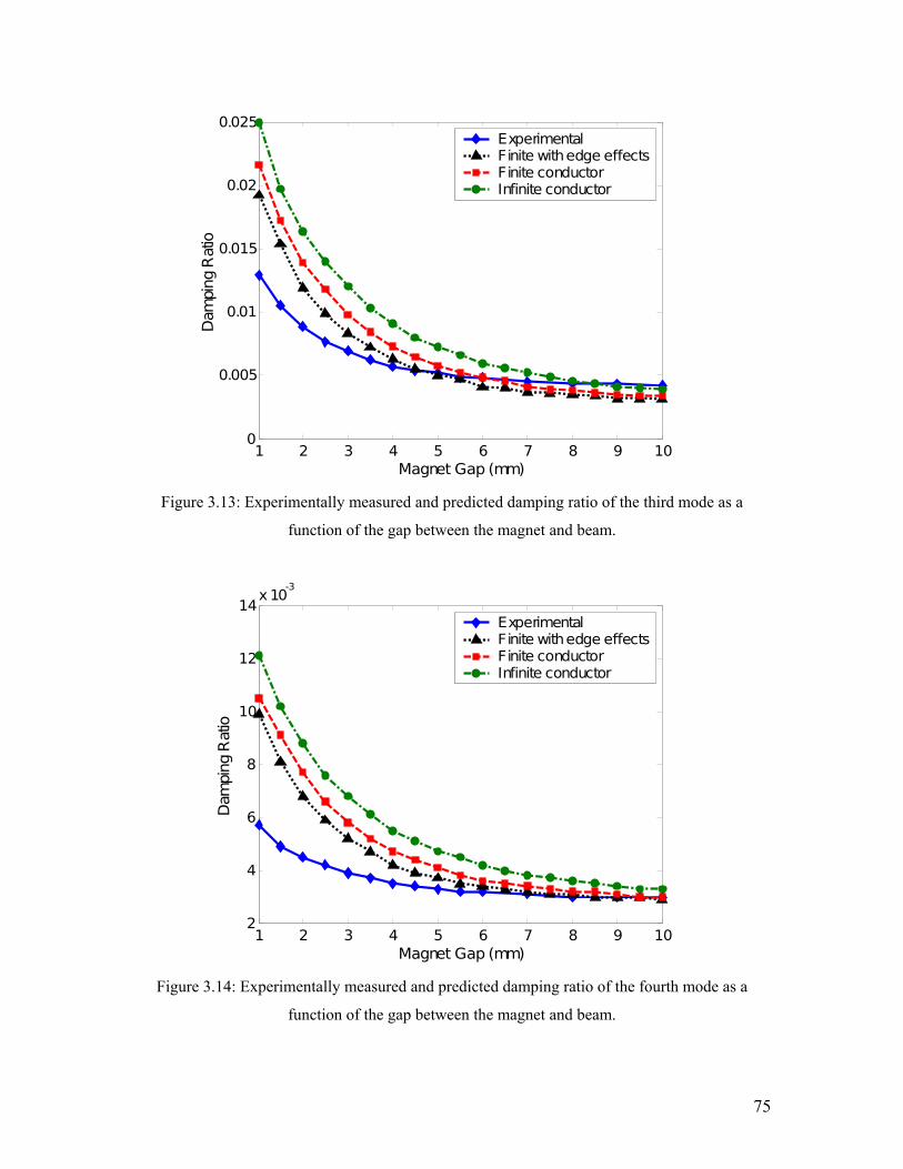
75

1 2 3 4 5 6 7 8 9 100

0.005

0.01

0.015

0.02

0.025

Magnet Gap (mm)

Dam

ping

Rat

io

ExperimentalFinite with edge effectsFinite conductorInfinite conductor

Figure 3.13: Experimentally measured and predicted damping ratio of the third mode as a

function of the gap between the magnet and beam.

1 2 3 4 5 6 7 8 9 102

4

6

8

10

12

14x 10

-3

Magnet Gap (mm)

Dam

ping

Rat

io

ExperimentalFinite with edge effectsFinite conductorInfinite conductor

Figure 3.14: Experimentally measured and predicted damping ratio of the fourth mode as a

function of the gap between the magnet and beam.

76

3.3 Experimental Testing and Results of the Improved

Passive Eddy Current Damper Concept

The derivation of the eddy current density performed in chapter 2 showed that the generation of

eddy currents was due to the radial magnetic flux of the permanent magnet. Using this idea it is

realized that when a permanent magnet is brought into close proximity with a second magnet of

the same polarity, the magnetic field is compressed in the poling direction. The compression of

the magnetic field results in an increase in the radial magnetic flux as shown in Figure 3.1. Due

to this increased magnetic flux in the radial direction, the use of a second magnet causes the

damping force to be significantly higher than the use of a single magnet. Additionally, when a

second magnet is incorporated into the design the system, the damping effect becomes more

linear than with a single magnet. This occurs because the flux on both sides of the beam is equal

the beam’s motion in each direction results in an equal generation of eddy currents and damping

force, where as with a single magnet, significantly more force results from motion in one

direction as the other. Using this concept and the superposition of the magnetic fields developed

in chapter 2, the following section will perform experiments on a cantilever beam to show the

increased damping effect and the accuracy of the modeling techniques when used to predict the

damping added to the structure.

3.3.1 Passive Eddy Current Damper Experimental Setup

Similar to the experiments performed in the previous section, the improved eddy current

damping concept was experimentally tested on a cantilever beam to identify the accuracy and

versatility of the modeling techniques developed in predicting the damping when a second

magnetic is incorporated into the system. Furthermore, the experiments performed will show the

improved performance of this damper. The dimensions of the cantilever beam were left the same

as those used in the previous section and shown in Figure 3.2, in order to allow a comparison

between the use of a single and two magnets to be made. The experiments used two neodymium-

iron-boron (NdFeB) permanent magnets with radius and length of 6.35mm and 12.7mm,

respectively. Other relevant properties of the beam and magnet are shown in Table 3.1. When

predicting the damping added to the structure, it was necessary to include the effect of the highly

conductor aluminum beam in the analysis.

77

To show the accuracy of the model, and performance of the damper, the damping ratio of the

beam was measured as the gap between the face of the magnet and the surface of the conductor

was varied. The improved concept utilizes two permanent magnets positioned on opposite sides

of the beam rather than a single magnet. The two magnets were configured such that the same

magnetic poles were facing each other causing a repulsive force between the magnets and causing

the magnetic flux to be compressed along the poling axis of the magnet. The compression of the

magnetic flux in this way causes its magnitude in the radial direction to be substantially increased

and thus the damping force is enhanced. The layout of the magnets is shown in Fig. 3.15.

Figure 3.15: Experimental setup showing position of magnets and conducting plates.

To measure the damping ratio of the beam as the distance between the magnet and the

conductor is varied, the frequency response was measured. The beam was excited using a

piezoelectric patch mounted at the root of the beam and the displacement response at the tip of

the beam was recorded using a Polytec Laser vibrometer. Once the frequency response of the

system was determined the UMPA was applied to the frequency response allowing the damping

ratio of the system to be extracted.

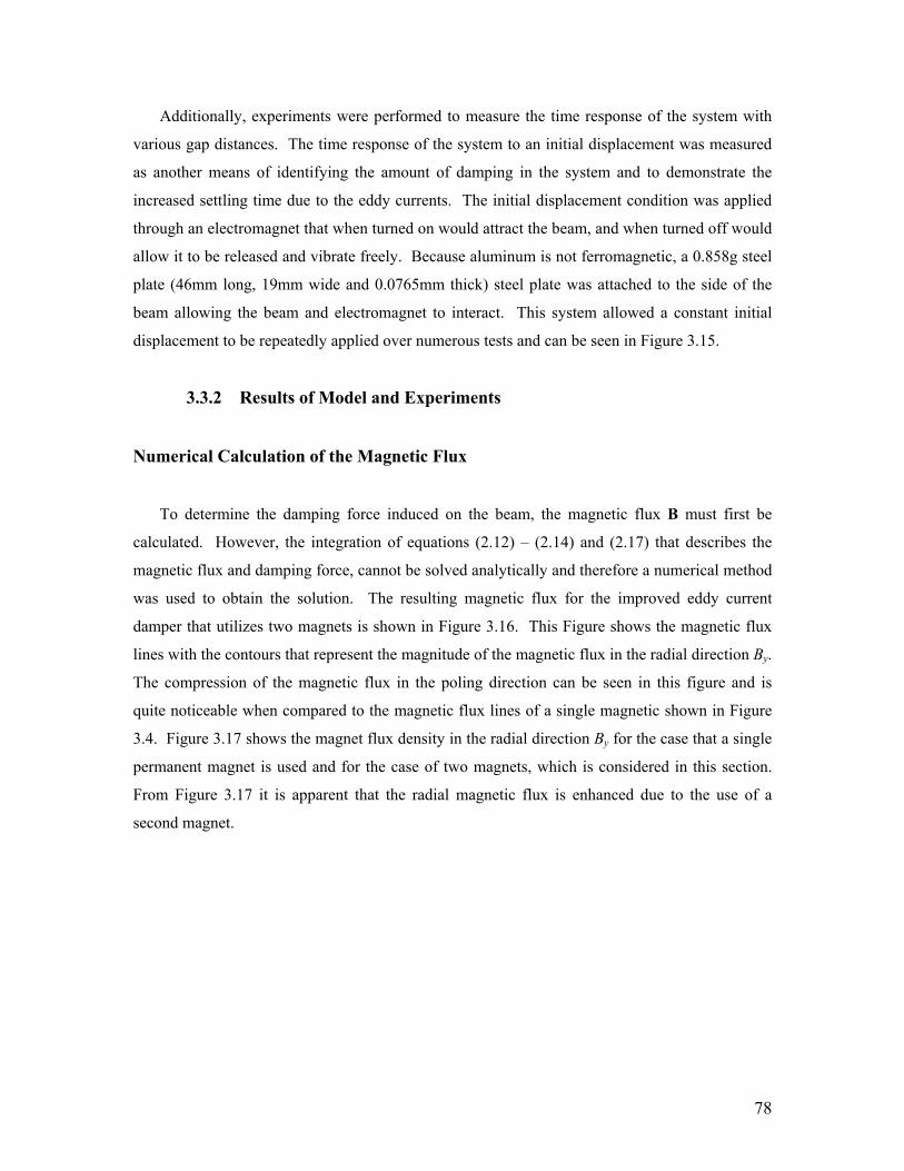
78

Additionally, experiments were performed to measure the time response of the system with

various gap distances. The time response of the system to an initial displacement was measured

as another means of identifying the amount of damping in the system and to demonstrate the

increased settling time due to the eddy currents. The initial displacement condition was applied

through an electromagnet that when turned on would attract the beam, and when turned off would

allow it to be released and vibrate freely. Because aluminum is not ferromagnetic, a 0.858g steel

plate (46mm long, 19mm wide and 0.0765mm thick) steel plate was attached to the side of the

beam allowing the beam and electromagnet to interact. This system allowed a constant initial

displacement to be repeatedly applied over numerous tests and can be seen in Figure 3.15.

3.3.2 Results of Model and Experiments

Numerical Calculation of the Magnetic Flux

To determine the damping force induced on the beam, the magnetic flux B must first be

calculated. However, the integration of equations (2.12) – (2.14) and (2.17) that describes the

magnetic flux and damping force, cannot be solved analytically and therefore a numerical method

was used to obtain the solution. The resulting magnetic flux for the improved eddy current

damper that utilizes two magnets is shown in Figure 3.16. This Figure shows the magnetic flux

lines with the contours that represent the magnitude of the magnetic flux in the radial direction By.

The compression of the magnetic flux in the poling direction can be seen in this figure and is

quite noticeable when compared to the magnetic flux lines of a single magnetic shown in Figure

3.4. Figure 3.17 shows the magnet flux density in the radial direction By for the case that a single

permanent magnet is used and for the case of two magnets, which is considered in this section.

From Figure 3.17 it is apparent that the radial magnetic flux is enhanced due to the use of a

second magnet.

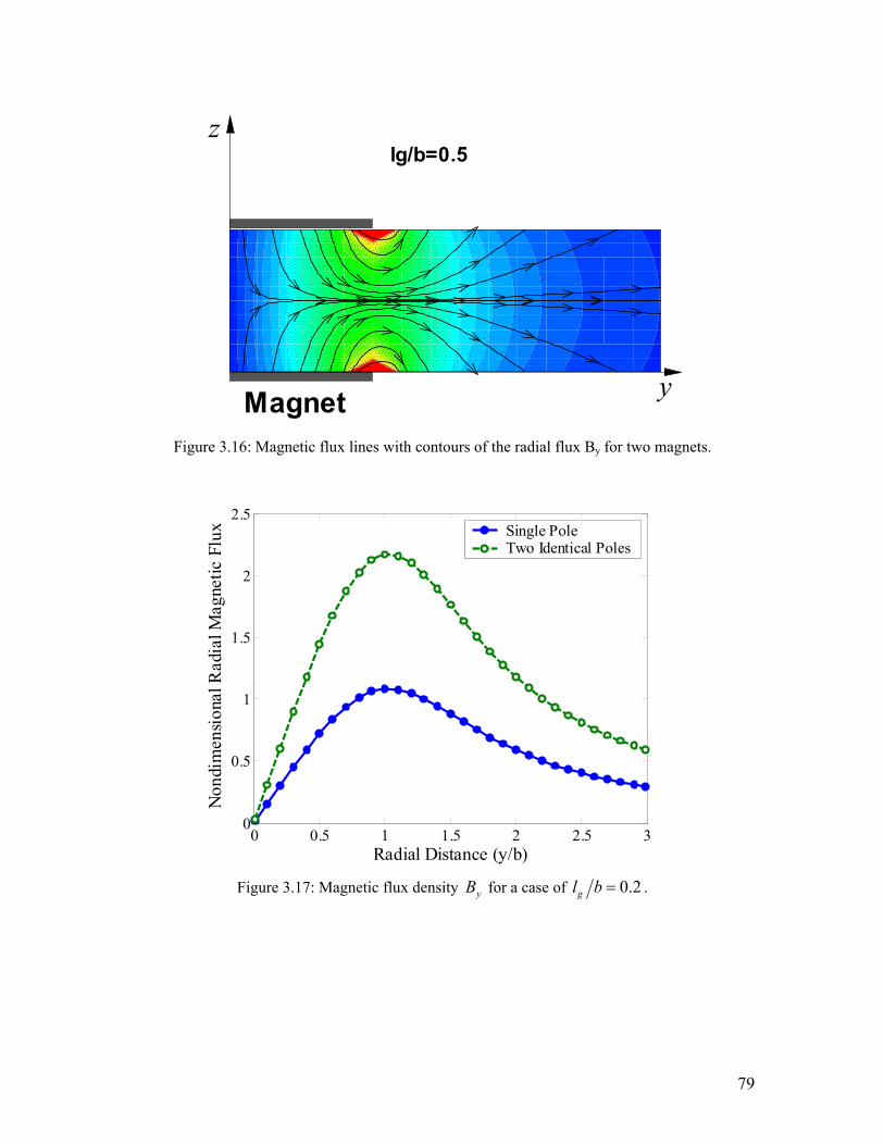
79

Magnet y

zlg/b=0.5

Figure 3.16: Magnetic flux lines with contours of the radial flux By for two magnets.

0 0.5 1 1.5 2 2.5 30

0.5

1

1.5

2

2.5

Radial Distance (y/b)

Non

dim

ensio

nal R

adia

l Mag

netic

Flu

x Single PoleTwo Identical Poles

Figure 3.17: Magnetic flux density yB for a case of 0.2gl b = .

80

Validation of Model through Experiments

Validation of the enhanced eddy damper model is performed by measuring the damping ratio

predicted by the model and the damping ratio measured in experiments. The performance of the

improved eddy current damper can be demonstrated by looking at the magnitude of the frequency

response function and the beam’s settling time to an initial displacement. In order to obtain the

damping ratio from the experimental data, the UMPA method was applied to the frequency

response. However, when performing the experiments it was found that the damping ratio of the

first mode was overdamped for the case that the magnets were in close proximity to the beam.

Therefore, in this gap range the time response of the beam when subjected to an initial

displacement was measured, thus allowing the log decrement to be calculated. One

experimentally obtained frequency response of the system before and after placement of both one

and two permanent magnets is shown in Figure 3.18. From this Figure it is apparent that the

damping of the structure is significantly increased after addition of the magnets into the system.

Additionally, the use of two magnets provides significantly more vibration reduction than when

one magnet is used. When two magnets are used and located 1mm from the conductor, the first

mode is overdamped and the magnitude is suppressed by approximately 54dB, the reduction in

the magnitude of the second, third and fourth modes are 31dB, 22.5dB and 14dB, respectively,

whereas when one magnet was used, the reduction in magnitude of the first, second and third

modes was 42.4dB, 21.9dB and 14.3dB, respectively. Furthermore, since this eddy current

damper does not contact the structure, significant damping can be added without changing the

dynamic response of the system, as can be seen in Figure 3.18. If other passive damping methods

such as constrained layer damping were to be used, the response of the structure would be

considerably altered due to a change in the mass and stiffness of the structure. The increased

damping through the use of two magnets can also be seen in Figure 3.19, which shows the time

response of the beam subjected to an initial displacement when one and two magnets are located a

distance of 2.5mm. These results indicate the advantage of using the new damper configuration

developed in this section for the suppression of transverse beam vibrations.

81

0 50 100 150 200 250 300 350 400-70

-60

-50

-40

-30

-20

-10

0

10

20

Frequency (Hz)

Mag

nitu

de (d

B)

UndampedDamped with two magnetsDamped with one magnet

Fig. 3.18: Experimentally obtained frequency response of the system before and after placement

of the magnets a distance of 1mm.

1.3 1.4 1.5 1.6 1.7 1.8 1.9 2-2

-1.5

-1

-0.5

0

0.5

1

1.5

2

2.5

Time (sec)

Dis

plac

emen

t (m

m)

Two MagnetsOne Magnet

Figure 3.19: Time response of the beam to an initial displacement when one and two magnets are

present at a distance of 2.5mm from the conductor.

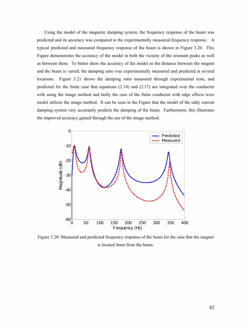
82

Using the model of the magnetic damping system, the frequency response of the beam was

predicted and its accuracy was compared to the experimentally measured frequency response. A

typical predicted and measured frequency response of the beam is shown in Figure 3.20. This

Figure demonstrates the accuracy of the model in both the vicinity of the resonant peaks as well

as between them. To better show the accuracy of the model as the distance between the magnet

and the beam is varied, the damping ratio was experimentally measured and predicted at several

locations. Figure 3.21 shows the damping ratio measured through experimental tests, and

predicted for the finite case that equations (2.14) and (2.17) are integrated over the conductor

with using the image method and lastly the case of the finite conductor with edge effects were

model utilizes the image method. It can be seen in the Figure that the model of the eddy current

damping system very accurately predicts the damping of the beam. Furthermore, this illustrates

the improved accuracy gained through the use of the image method.

0 50 100 150 200 250 300 350 400-60

-50

-40

-30

-20

-10

0

Frequency (Hz)

Mag

nitu

de (dB

)

P redictedMeasured

Figure 3.20: Measured and predicted frequency response of the beam for the case that the magnet

is located 4mm from the beam.

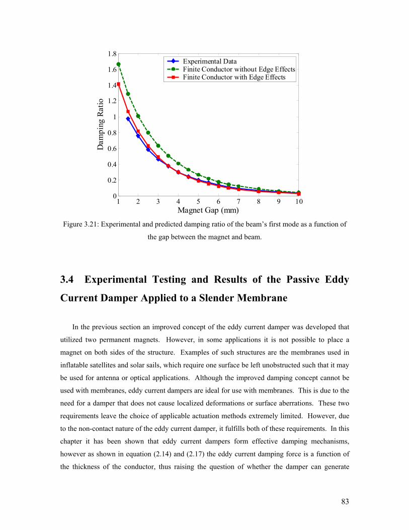
83

1 2 3 4 5 6 7 8 9 100

0.2

0.4

0.6

0.8

1

1.2

1.4

1.6

1.8

Magnet Gap (mm)

Dam

ping

Rat

io

Experimental DataFinite Conductor without Edge EffectsFinite Conductor with Edge Effects

Figure 3.21: Experimental and predicted damping ratio of the beam’s first mode as a function of

the gap between the magnet and beam.

3.4 Experimental Testing and Results of the Passive Eddy

Current Damper Applied to a Slender Membrane

In the previous section an improved concept of the eddy current damper was developed that

utilized two permanent magnets. However, in some applications it is not possible to place a

magnet on both sides of the structure. Examples of such structures are the membranes used in

inflatable satellites and solar sails, which require one surface be left unobstructed such that it may

be used for antenna or optical applications. Although the improved damping concept cannot be

used with membranes, eddy current dampers are ideal for use with membranes. This is due to the

need for a damper that does not cause localized deformations or surface aberrations. These two

requirements leave the choice of applicable actuation methods extremely limited. However, due

to the non-contact nature of the eddy current damper, it fulfills both of these requirements. In this

chapter it has been shown that eddy current dampers form effective damping mechanisms,

however as shown in equation (2.14) and (2.17) the eddy current damping force is a function of

the thickness of the conductor, thus raising the question of whether the damper can generate

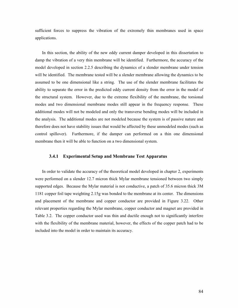
84

sufficient forces to suppress the vibration of the extremely thin membranes used in space

applications.

In this section, the ability of the new eddy current damper developed in this dissertation to

damp the vibration of a very thin membrane will be identified. Furthermore, the accuracy of the

model developed in section 2.2.5 describing the dynamics of a slender membrane under tension

will be identified. The membrane tested will be a slender membrane allowing the dynamics to be

assumed to be one dimensional like a string. The use of the slender membrane facilitates the

ability to separate the error in the predicted eddy current density from the error in the model of

the structural system. However, due to the extreme flexibility of the membrane, the torsional

modes and two dimensional membrane modes still appear in the frequency response. These

additional modes will not be modeled and only the transverse bending modes will be included in

the analysis. The additional modes are not modeled because the system is of passive nature and

therefore does not have stability issues that would be affected by these unmodeled modes (such as

control spillover). Furthermore, if the damper can performed on a thin one dimensional

membrane then it will be able to function on a two dimensional system.

3.4.1 Experimental Setup and Membrane Test Apparatus

In order to validate the accuracy of the theoretical model developed in chapter 2, experiments

were performed on a slender 12.7 micron thick Mylar membrane tensioned between two simply

supported edges. Because the Mylar material is not conductive, a patch of 35.6 micron thick 3M

1181 copper foil tape weighting 2.15g was bonded to the membrane at its center. The dimensions

and placement of the membrane and copper conductor are provided in Figure 3.22. Other

relevant properties regarding the Mylar membrane, copper conductor and magnet are provided in

Table 3.2. The copper conductor used was thin and ductile enough not to significantly interfere

with the flexibility of the membrane material, however, the effects of the copper patch had to be

included into the model in order to maintain its accuracy.

85

Figure 3.22: Dimensions of membrane strip and location of copper conductor.

Table 3.2: Physical properties of the beam, conductor and magnet.

Property Value

Young’s modulus of Mylar membrane 4.7 GPa

Density of Mylar membrane 1390 kg/m3

Young’s modulus of copper conductor 131 x 107 mho/m

Density of copper conductor 8910 kg/m3

Conductivity of copper conductor 1. 052 x 107 mho/m

Permanent magnet composition NdFeB 45

Residual magnetic flux of magnet 1.35 kGauss

The goals of the experiments performed in this study are to identify the damping ratio and

frequency response of the slender membrane subjected to an axial load when at vacuum and

ambient pressure. However, experimentally testing a membrane structure is very difficult due to

the limited choice of sensing and actuation methods, wrinkling, modal coupling and the

sensitivity to both boundary conditions and air currents. The boundary conditions of the

membrane are chosen to be pinned in order to maintain constant eigenfunctions as axial tension is

applied (Shaker, 1975). The pinned boundary conditions were constructed by clamping the edge

of the membrane strip between two 6.35 mm diameter steel rods, similar to the clamps used by

Hall et al. (2002). The axial load was applied to the membrane by attaching one of the pinned

boundary conditions to a Velmex unislide lead screw, while the other pinned boundary condition

was fixed to a Transducer Techniques MLP-75 load cell that measured the force applied to the

membrane by the lead screw, as shown in Figure 3.23. By monitoring the load cell reading and

adjusting the lead screw, the tension in the membrane could be accurately set. Due to the very

high flexibility of the membrane, both sensing and actuation techniques must be carefully chosen.

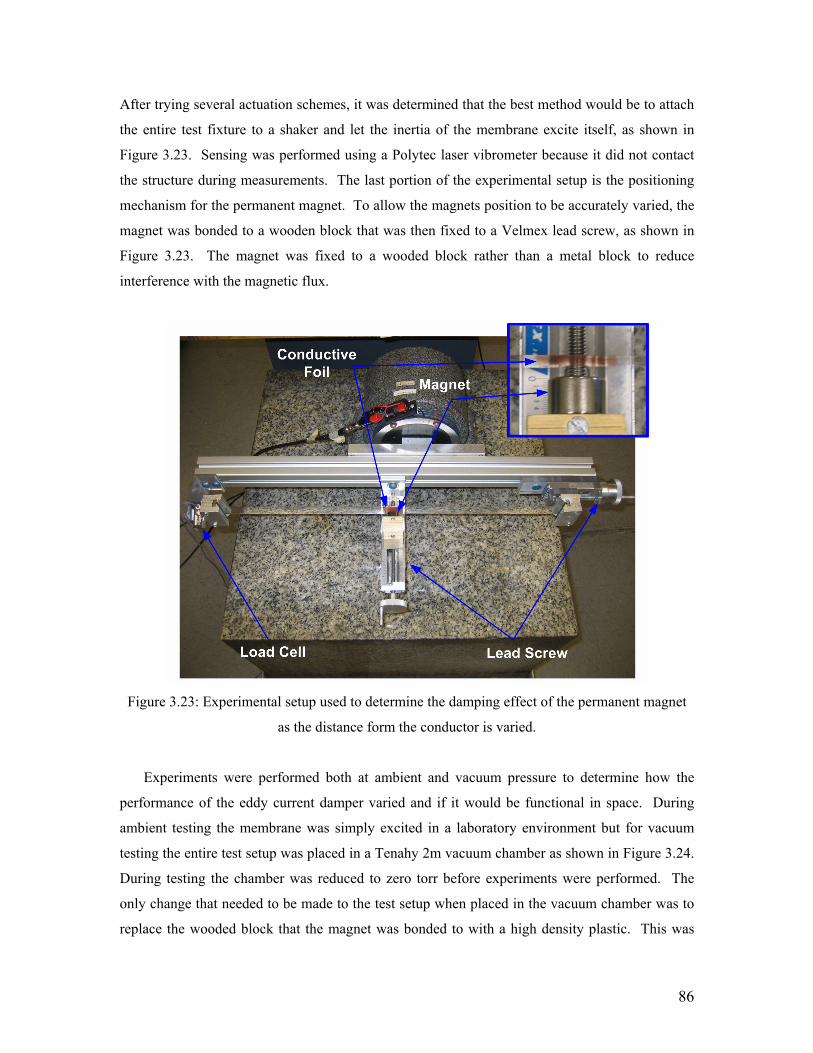
86

After trying several actuation schemes, it was determined that the best method would be to attach

the entire test fixture to a shaker and let the inertia of the membrane excite itself, as shown in

Figure 3.23. Sensing was performed using a Polytec laser vibrometer because it did not contact

the structure during measurements. The last portion of the experimental setup is the positioning

mechanism for the permanent magnet. To allow the magnets position to be accurately varied, the

magnet was bonded to a wooden block that was then fixed to a Velmex lead screw, as shown in

Figure 3.23. The magnet was fixed to a wooded block rather than a metal block to reduce

interference with the magnetic flux.

Figure 3.23: Experimental setup used to determine the damping effect of the permanent magnet

as the distance form the conductor is varied.

Experiments were performed both at ambient and vacuum pressure to determine how the

performance of the eddy current damper varied and if it would be functional in space. During

ambient testing the membrane was simply excited in a laboratory environment but for vacuum

testing the entire test setup was placed in a Tenahy 2m vacuum chamber as shown in Figure 3.24.

During testing the chamber was reduced to zero torr before experiments were performed. The

only change that needed to be made to the test setup when placed in the vacuum chamber was to

replace the wooded block that the magnet was bonded to with a high density plastic. This was

87

required because as the air was removed from the chamber the moisture in the wooden block was

also removed causing the block to shrink. The vacuum chamber had a glass window that allowed

the laser vibrometer to be used for measuring the membranes vibration. It was found through

experiments that the glass window did not affect the quality of the measured data, but rather, the

data’s quality was actually improved due to the isolation from air currents in the chamber.

Figure 3.24: Experimental setup in the vacuum chamber.

3.4.2 Results of the Model and Experiments

The scope of this research is to show the ability of the passive eddy current damping system

developed in this dissertation to add significant damping to a thin membrane structure and

develop an accurate model of the damping mechanism’s interaction with the membrane. The

ability of the eddy current damping system to add damping into the structure is shown by

measuring the frequency response before and after placement of the magnet. Figure 3.25, shows

the frequency response of the membrane when the eddy current damper is not present in the

system and for the case that the magnet is located a distance of 1mm from the membrane’s

surface. To help identify the modes shown in Figure 3.25, the frequencies are labeled B1 for the

first bending mode, B2 for the second bending, T1 for the first torsional and so on. Additionally,

Table 3.3 provides the frequencies of each of the first four bending modes and the first three

torsional modes when the membrane is at both ambient and vacuum pressure. The frequencies

presented in Table 3.3 were identified by performing a modal analysis on the structure. It can be

seen from Figure 3.25 that the damper provides significant damping to the membrane, reducing

the magnitude of the first bending mode by 13.7 dB and the third bending mode by 5.2 dB. The

88

second and fourth bending modes do not show any additional damping because the magnet is

located at the center of the membrane strip which is a nodal point for these modes.

0 50 100 150 200 250 300 350-30

-25

-20

-15

-10

-5

0

5

10

Frequency (Hz)

Mag

nitu

de (dB

)DampedUndamped

B1

B2

T1

T2 T3

B3

B4

Figure 3.25: Measured frequency response without magnet and with magnet a distance of 1mm

from membrane at ambient pressure.

Table 3.3: Bending and torsional natural frequencies of the membrane with a tension of 8.9N at

both vacuum and ambient pressure.

Mode Shape Ambient Pressure Vacuum Pressure

First Bending (B1) 62 Hz 71.7 Hz

First Torsional (T1) 88.5 Hz 157 Hz

Second Bending (B2) 154 Hz 194.5 Hz

Second Torsion (T2) 178 Hz 212 Hz

Third Bending (B3) 205.8 Hz 242.5 Hz

Third Torsion (T3) 249 Hz 326 Hz

Fourth Bending (B4) 307.5 Hz 379.7 Hz

During tests on the membrane at vacuum conditions it was found that the eddy current

damping system reduces the magnitude of the response better than at ambient conditions. The

89

frequency response of the membrane when the damping mechanism was not present and when the

magnet is located 1mm from the surface of the membrane is shown in Figure 3.26. From the

figure it can be seen that the magnitude of the first bending mode is reduced by 31.06 dB and the

third bending mode by 15.62 dB. As with the ambient tests the second and forth bending

frequencies are not damped by the magnet because it is located at a nodal point of the modes.

Additionally, a slight shift occurs in the second and fourth mode due to the hygroscopic effects of

the polymer which will be discussed later.

0 50 100 150 200 250 300 350 400 450-50

-40

-30

-20

-10

0

10

20

Frequency (Hz)

Mag

nitu

de (dB

)

DampedUndamped

B1

B2 B3

B4

Figure 3.26: Measured frequency response without magnet and with magnet a distance of 1mm

from membrane at vacuum pressure and at an axial load of 8.9N.

While the damper performs well at vacuum conditions, the dynamic response of the

membrane changes fairly significantly when subjected to vacuum pressure. The change in the

frequency response of the membrane between ambient and vacuum pressure are compared in

Figure 3.27, and the shift in natural frequency for each mode can be seen in Table 3.3. The

change in dynamic response can be attributed to the hygroscopic effects of the Mylar material and

the decreased damping from the removal of air. The hygroscopic effects occur due to the

moisture in the polymer Mylar material being expelled as the pressure drops to vacuum. This

causes the polymer material to shrink and the tension applied to the membrane to increase. The

increase in tension was measured using the load cell, but the effect on other material properties

90

such the elastic modulus and density, could not be measured and therefore, could not be included

in the theoretical model of the system. For more information on the hygroscopic effect of

polymers at vacuum pressure see Bales et al. (2003). The amount of damping present in the

system was determined by applying the UMPA to the frequency response data. Using the UMPA

method, the damping ratio of the membrane system was determined for the magnet being placed

at various distances from the membrane surface in both ambient and vacuum conditions. The

resulting damping ratio of the membrane for each case is shown in Figure 3.28. As can be seen in

the figure the damping ratio maintains almost a constant offset of approximately 0.025 over the

tested range. The decrease in damping when the membrane is placed in a vacuum can be

attributed to lack of air damping which can make a significant difference in lightweight structures

such as membranes.

0 50 100 150 200 250 300 350 400 450-50

-40

-30

-20

-10

0

10

Frequency (Hz)

Mag

nitu

de (dB

)

Ambient PressureVacuum Pressure

Figure 3.27: Measured frequency response at ambient and vacuum pressure with magnet gap of

2mm and an axial load of 8.9N.

91

1 2 3 4 5 6 7 8 9 100

0.05

0.1

0.15

0.2

0.25

0.3

0.35

Magnet Gap (mm)

Dam

ping

Rat

io

Measured AmbientMeasured Vacuum

Figure 3.28: Measured damping ratio of membrane at both ambient and vacuum pressure with an

axial load of 8.9N.

After testing the performance of the eddy current damper at both ambient and vacuum

conditions the accuracy of the model could be validated against the measured data. Using the

model of the eddy current damping system that was been developed in chapter 2, the frequency

response of the membrane could be predicted as a function of the gap between the magnet and the

membrane surface. The predicted and measured damping ratio for the membrane at ambient

pressure for various gaps between the magnet and the membrane surface are shown in Figure

3.29. It can be seen from the figure that the model accurately predicts the damping ratio over the

entire range of gap lengths.

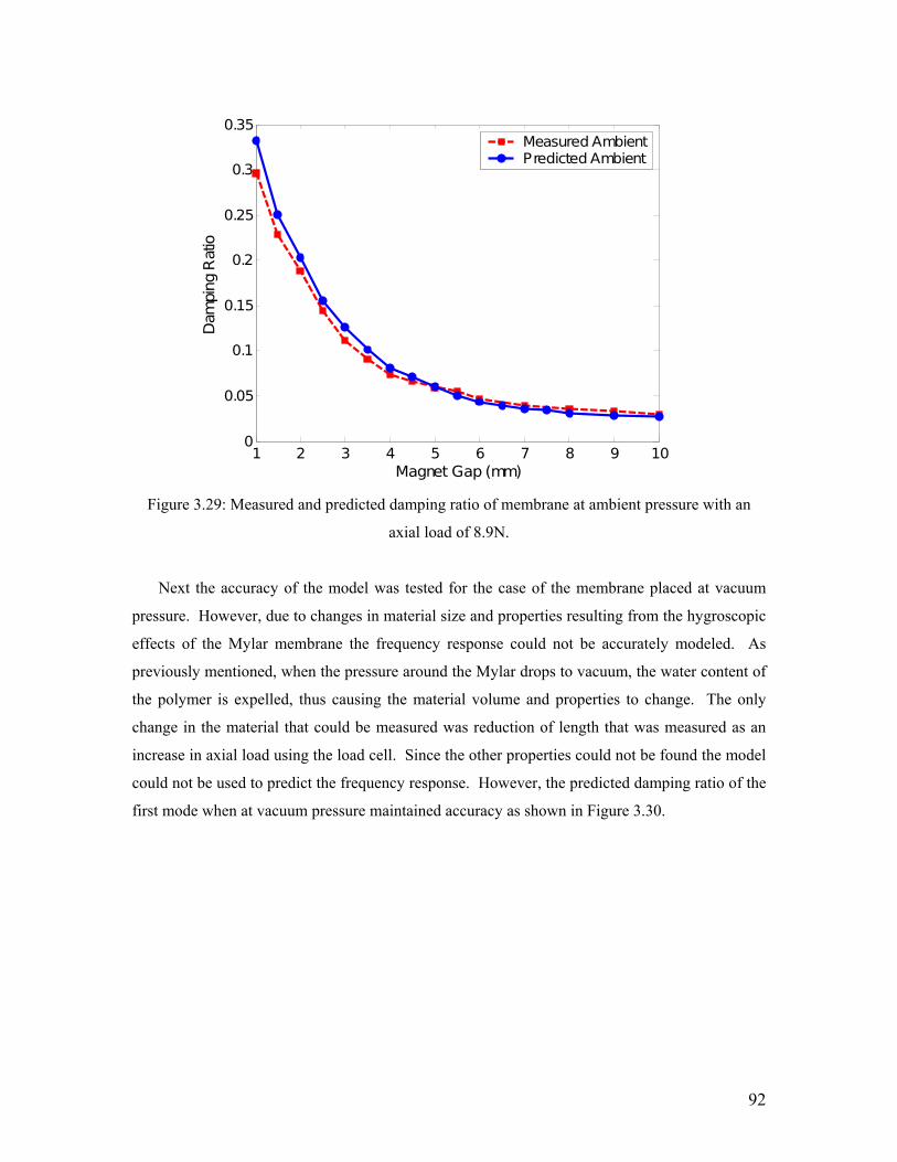
92

1 2 3 4 5 6 7 8 9 100

0.05

0.1

0.15

0.2

0.25

0.3

0.35

Magnet Gap (mm)

Dam

ping

Rat

io

Measured AmbientPredicted Ambient

Figure 3.29: Measured and predicted damping ratio of membrane at ambient pressure with an

axial load of 8.9N.

Next the accuracy of the model was tested for the case of the membrane placed at vacuum

pressure. However, due to changes in material size and properties resulting from the hygroscopic

effects of the Mylar membrane the frequency response could not be accurately modeled. As

previously mentioned, when the pressure around the Mylar drops to vacuum, the water content of

the polymer is expelled, thus causing the material volume and properties to change. The only

change in the material that could be measured was reduction of length that was measured as an

increase in axial load using the load cell. Since the other properties could not be found the model

could not be used to predict the frequency response. However, the predicted damping ratio of the

first mode when at vacuum pressure maintained accuracy as shown in Figure 3.30.

93

1 2 3 4 5 6 7 8 9 100

0.05

0.1

0.15

0.2

0.25

0.3

0.35

Magnet Gap (mm)

Dam

ping

Rat

io

Measured VacuumPredicted Vacuum

Figure 3.30: Measured and predicted damping ratio of membrane at vacuum pressure with an

axial load of 8.9N.

This damping mechanism has several advantages over other methods of applying damping to

the membrane. Because the intended use of this technology is to damp the vibrations of optical or

antenna membranes, the surface must remain flat, which limits the type of damping devices that

can be used. This point brings up one of the major advantages of this type of damping

mechanism; the damper is non-contact and therefore does not cause inconsistencies on the

membrane surface that would arise from bonding. The damper also applies a distributed force on

the surface of the membrane which is necessary to achieve global damping and avoid local

deformation. Furthermore, because the damper is non-contact it does not change the dynamic

response of the system which can be seen in Figures 3.25 and 3.26. Another advantage of this

type of damper is that it is extremely easy to install and only modifies the system damping.

Additionally, Magnetic dampers do not require any maintenance to stay functional, which is a

very important trait of any space system. For these reasons, magnetic damping mechanisms are

an excellent choice for use in space.

94

3.5 Chapter Summary

Eddy currents form an effective means of applying damping to a vibrating structure. However

they have generally been used for magnetic braking applications and those that have been aimed

at vibration suppression are typically ineffective at suppressing structural vibration, not

compatible with practical systems, or cumbersome to the structure resulting in significant mass

loading and changes to the dynamic response. To alleviate these issues, a new passive damping

mechanism has been developed. This damper functions by placing a permanent magnet a small

distance from a vibrating beam such that the beams motion is along the poling axes of the

magnet. Because the magnet does not contact the beam the damper is easy to install.

Furthermore, because the damper is non-contacting, it can be implemented without causing the

mass loading and added stiffness, which are common downfalls of other damping methods. By

avoiding mass loading and added stiffness, the damper does not change the mode shapes or

natural frequencies of the system, which is an important trait for those systems designed to have a

particular dynamic response but require additional damping after their design. The non-contact

nature of this system is also advantageous for providing damping to extremely flexible structures

such as membranes that would experience local deformations or surface irregularities if a

conventional damper were used. However, this damper has the limitation that a structure to

support the magnet must be included in the design.

The new damper configuration was theoretically modeled in chapter 2. This chapter began

by deriving the damping force, then incorporating the image method into the solution to enforce a

zero eddy current boundary condition (Lee and Park, 2002). After identifying the damping force,

the equations of motion for a beam and a slender membrane under tension were developed with

the effect of the eddy current damper included in the response. Once the theoretical models

required to predict the response of the beam had been developed, it was necessary to identify their

accuracy. Therefore, chapter 3 has developed several experiments to validate the accuracy of the

models developed in chapter 2.

First a cantilever beam was configured such that a permanent magnet was located a small

distance from a conductive patch bonded to the beam’s surface. The magnet was fixed to a lead

screw that allowed its position to be accurately changed and thus the damping ratio of the beam to

be determined as the position of the magnet is varied. The model was shown to accurately predict

the damping ratio on average with an error less than 13%. Furthermore, the use of a single

95

magnet was shown to increase the damping ratio of the first mode up to 0.35. Following the

results using a single magnet, the concept that the radial magnetic flux is responsible for the

generation of the eddy currents, which was identified in chapter 2, was used to improve the

dampers performance. By placing a second magnet on the opposite side of the beam, such that

similar poles were facing each other, the magnetic field in the radial direction could be magnified

and thus the eddy current density and damping force could be enhanced. This system was

experimentally tested and shown to match the models predictions very well, with the predicted

damping on average within 10%. Additionally, it was shown that the damping could be

significantly increased to the point that the cantilever beam’s fundamental mode of vibration

could be critically damped. The third experiment performed was on a thin slender membrane in

order to validate the ability of the eddy current damper to suppress the vibration of an extremely

thin structure. It was questionable as to the dampers performance on a thin structure because the

damping force is proportional to the thickness of the conductive material. However, it was shown

through experiments that the model accurately predicted the damping induced on the 12.7 micron

thick membrane and was able to suppress the vibration of the first mode by more than 97%.

96

Chapter 4

Development of a New Passive-Active

Magnetic Damper

4.1 Passive-Active Damper Concept

In chapters two and three, a new passive eddy current damping concept was developed and

modeled. This passive damping system functioned through the eddy currents that were formed in

the conductive beam due to its motion in a static magnetic field. As the beam vibrated in the

magnetic field, it was subjected to a time-varying magnetic flux that induced an electromotive

force (emf) causing eddy currents to form and circulate. The model developed in chapter two

showed that the density of the eddy currents, and the damping force generated, were a function of

the velocity of the beam in the magnetic field. To capitalize on this concept, this chapter will

develop a novel passive-active damping mechanism that consists of a permanent magnet which is

free to move relative to the beam. The passive component of this new system is the motion of the

beam in the static magnetic field, while an active component is added by controlling the position

of the magnet relative to the beam. By monitoring the beams motion and actively displacing the

magnet accordingly, the net velocity between the permanent magnet and the beam can be

controlled such that the damping applied to the beam can be maximized.

The passive-active nature of this system allows this damping mechanism to still be effective

as a passive device by leaving the magnet stationary. However when introducing active control

into a system, both advantages and disadvantages occur. The advantages of active control are

that specific frequencies can be targeted and vibration suppression can be achieved for various

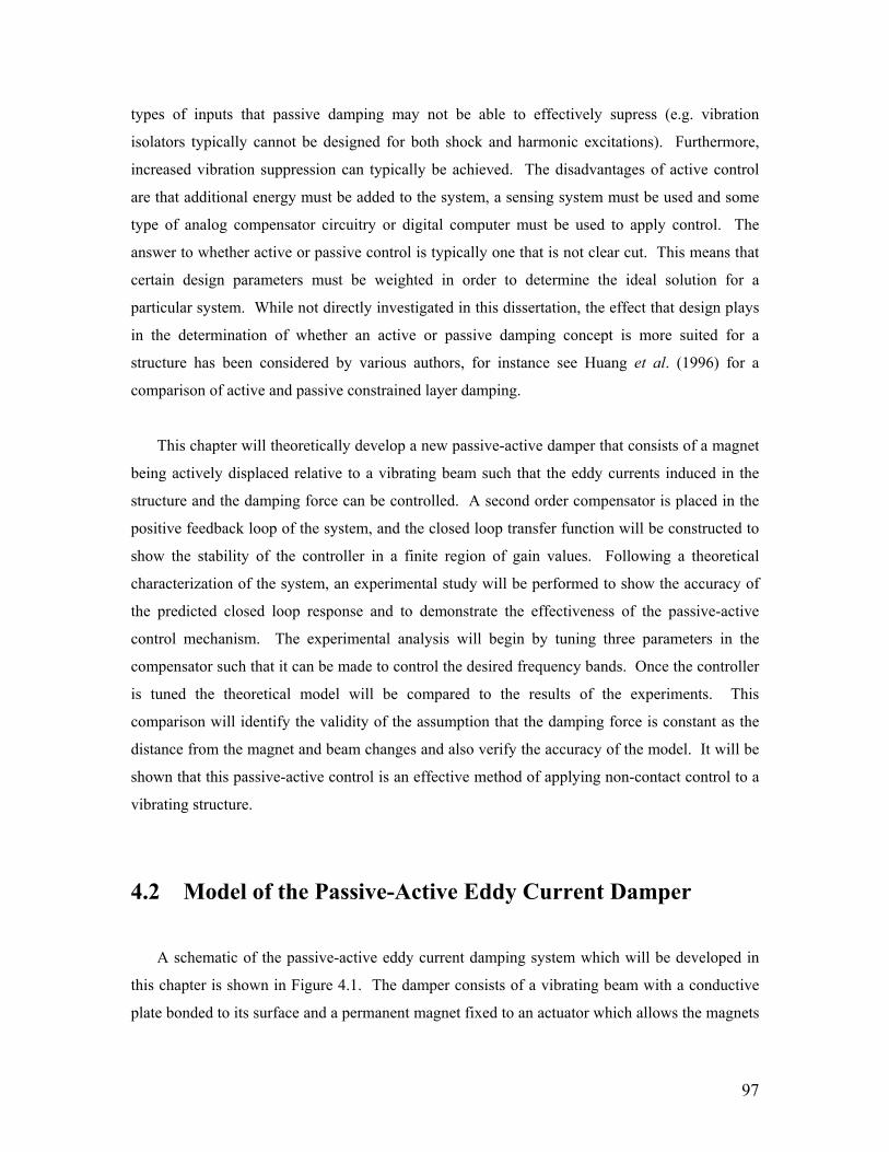
97

types of inputs that passive damping may not be able to effectively supress (e.g. vibration

isolators typically cannot be designed for both shock and harmonic excitations). Furthermore,

increased vibration suppression can typically be achieved. The disadvantages of active control

are that additional energy must be added to the system, a sensing system must be used and some

type of analog compensator circuitry or digital computer must be used to apply control. The

answer to whether active or passive control is typically one that is not clear cut. This means that

certain design parameters must be weighted in order to determine the ideal solution for a

particular system. While not directly investigated in this dissertation, the effect that design plays

in the determination of whether an active or passive damping concept is more suited for a

structure has been considered by various authors, for instance see Huang et al. (1996) for a

comparison of active and passive constrained layer damping.

This chapter will theoretically develop a new passive-active damper that consists of a magnet

being actively displaced relative to a vibrating beam such that the eddy currents induced in the

structure and the damping force can be controlled. A second order compensator is placed in the

positive feedback loop of the system, and the closed loop transfer function will be constructed to

show the stability of the controller in a finite region of gain values. Following a theoretical

characterization of the system, an experimental study will be performed to show the accuracy of

the predicted closed loop response and to demonstrate the effectiveness of the passive-active

control mechanism. The experimental analysis will begin by tuning three parameters in the

compensator such that it can be made to control the desired frequency bands. Once the controller

is tuned the theoretical model will be compared to the results of the experiments. This

comparison will identify the validity of the assumption that the damping force is constant as the

distance from the magnet and beam changes and also verify the accuracy of the model. It will be

shown that this passive-active control is an effective method of applying non-contact control to a

vibrating structure.

4.2 Model of the Passive-Active Eddy Current Damper

A schematic of the passive-active eddy current damping system which will be developed in

this chapter is shown in Figure 4.1. The damper consists of a vibrating beam with a conductive

plate bonded to its surface and a permanent magnet fixed to an actuator which allows the magnets

98

position to be actively controlled. The eddy currents are formed due to the net velocity between

the magnet and the beam occurring from the vibration of the beam and the active control applied

to the position of the magnet. Because the motion of the beam and the magnet lie on the same

axis as the poling direction of the magnet, the radial magnetic flux is responsible for the

formation of the eddy currents in the conductive material. The eddy current damping force will

be calculated first, followed by the dynamics of the beam and the coupling of these forces into its

response. The active controller will be a second order filter that is similar to that of a positive

position feedback controller (Fanson and Caughey, 1987) with the modification that the input is a

velocity and the output is the displacement of the magnet.

Figure 4.1: Cantilever beam in magnetic field generated by permanent magnet.

4.2.1 Model of the Eddy Current Damping Force

The symmetry of the circular permanent magnet allows the surface charges to be ignored and

thus the eddy current density J induced in the conductive sheet can be written as

99

( )BvJ ×= σ (4.1)

where the ×v B term is the cross product of the velocity v of the conductor and the magnetic

flux density B defining the electromotive force driving the eddy currents J. The velocity and

magnetic flux can be written as follows

( )kjiv mb vv −++= 00 (4.2)

kjiB zyx BBB ++= (4.3)

where the velocity of the beam vb and the velocity of the magnet vm are only in the z-direction.

After substitution of equations (2) and (3) into equation (1), the eddy current density is defined by

( ) ( )( )jiBvJ xymb BBvv +−−=×= σσ (4.4)

The above equation confirms that the magnetic flux in the z-direction has no effect on the induced

eddy currents and that the induced currents are solely dependent on the x- and y-components of

the magnetic flux or the flux tangential to the face of the conducting sheet.

In order to determine the eddy current density in the conducting sheet, the magnetic flux of

the permanent magnet must be found. For the case of a cylindrical permanent magnet, the

equation defining the flux density has been derived in chapter 2, thus only the resulting equations

for the magnetic flux density of the permanent magnet will be provided. The radial and

transverse magnetic flux density due to the circular magnet of length L are written by

( ) ( ) ( )∫− ′′−′−=0

100 ,,

4,

Ly zdzzybIzzbMzyBπ

µ (4.5)

( ) ( )∫− ′′−=0

200 ,,

4,

Lz zdzzybIbMzyBπ

µ (4.6)

where 'z is the distance in the z direction from the center of a magnetized infinitesimal strip, L is

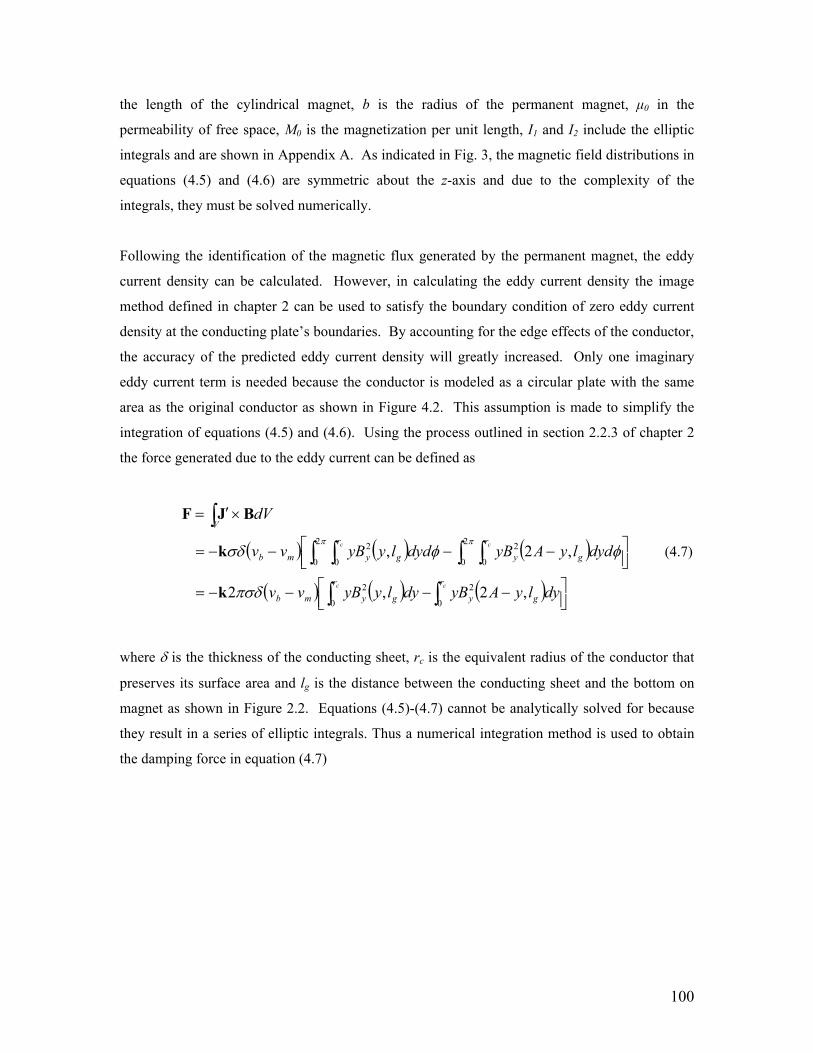
100

the length of the cylindrical magnet, b is the radius of the permanent magnet, µ0 in the

permeability of free space, M0 is the magnetization per unit length, I1 and I2 include the elliptic

integrals and are shown in Appendix A. As indicated in Fig. 3, the magnetic field distributions in

equations (4.5) and (4.6) are symmetric about the z-axis and due to the complexity of the

integrals, they must be solved numerically.

Following the identification of the magnetic flux generated by the permanent magnet, the eddy

current density can be calculated. However, in calculating the eddy current density the image

method defined in chapter 2 can be used to satisfy the boundary condition of zero eddy current

density at the conducting plate’s boundaries. By accounting for the edge effects of the conductor,

the accuracy of the predicted eddy current density will greatly increased. Only one imaginary

eddy current term is needed because the conductor is modeled as a circular plate with the same

area as the original conductor as shown in Figure 4.2. This assumption is made to simplify the

integration of equations (4.5) and (4.6). Using the process outlined in section 2.2.3 of chapter 2

the force generated due to the eddy current can be defined as

( ) ( ) ( )

( ) ( ) ( ) ⎥⎦⎤

⎢⎣⎡ −−−−=

⎥⎦⎤

⎢⎣⎡ −−−−=

×′=

∫∫

∫ ∫∫ ∫

∫

cc

cc

r

gy

r

gymb

g

r

yg

r

ymb

V

dylyAyBdylyyBvv

dydlyAyBdydlyyBvv

dV

0

2

0

2

2

0 0

22

0 0

2

,2,2

,2,

πσδ

φφσδππ

k

k

BJF

(4.7)

where δ is the thickness of the conducting sheet, rc is the equivalent radius of the conductor that

preserves its surface area and lg is the distance between the conducting sheet and the bottom on

magnet as shown in Figure 2.2. Equations (4.5)-(4.7) cannot be analytically solved for because

they result in a series of elliptic integrals. Thus a numerical integration method is used to obtain

the damping force in equation (4.7)

101

Figure 4.2: schematic showing the variables associated with the conducting plate.

4.2.2 Modeling of Cantilever Beam

The damping force calculated in equation (4.7) can now be incorporated into the dynamics of

the structure that the damper is to be applied to. For this analysis, a cantilever beam will be

studied. The equation of motion defining the dynamics of a cantilever beam were derived in

section 2.2.4 of chapter 2, and are written as

( ) ( ) ( ) ( ) ( ) ( ) ( )∫ ∑=

+=++L p

iii xtFdxxtxftrtrtr

01

, φφKCM (4.8)

where the mass matrix M, the damping matrix C, and the stiffness matrix K are defined by

( ) ( ) ( )∫==L T

ij dxxxxm0

φφρM (4.9)

( ) ( ) ( )∫ ′′′′==L T

ij dxxxxEIk0

φφK (4.10)

( )[ ][ ]eeij xcdiagc φ+== bCC (4.11)

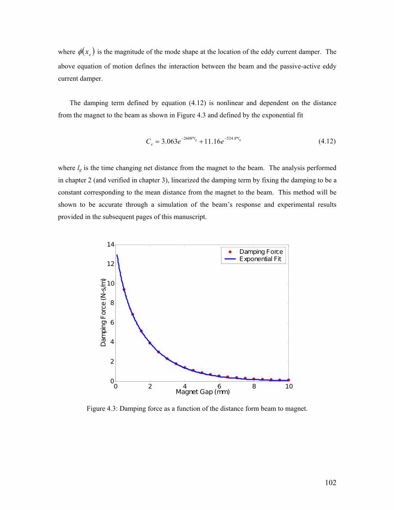
102

where ( )exφ is the magnitude of the mode shape at the location of the eddy current damper. The

above equation of motion defines the interaction between the beam and the passive-active eddy

current damper.

The damping term defined by equation (4.12) is nonlinear and dependent on the distance

from the magnet to the beam as shown in Figure 4.3 and defined by the exponential fit

gg ll

e eeC *8.524*2608 16.11063.3 −− += (4.12)

where lg is the time changing net distance from the magnet to the beam. The analysis performed

in chapter 2 (and verified in chapter 3), linearized the damping term by fixing the damping to be a

constant corresponding to the mean distance from the magnet to the beam. This method will be

shown to be accurate through a simulation of the beam’s response and experimental results

provided in the subsequent pages of this manuscript.

0 2 4 6 8 100

2

4

6

8

10

12

14

Magnet Gap (mm)

Dam

ping

For

ce (N

-s/m

)

Damping ForceExponential Fit

Figure 4.3: Damping force as a function of the distance form beam to magnet.

103

4.2.3 Controller Design

The position of magnet relative to the beam is actively controlled using a positive feedback

control law (Fanson and Caughey, 1987). The feedback controller is a second order filter with

three parameters chosen to provide the greatest vibration suppression of the frequency response.

The filter is defined by the following equation

22

2

2 fff

f

ssK

ωωζω

++ (4.13)

where K is the controller gain, ωf is the filter frequency and ζf is the filter damping ratio. The

compensator defined by equation (4.13) contains an extra zero in the numerator to account for the

dynamics of the electromagnetic actuator used to actively displace the magnet. The effective

bandwidth of the shaker is limited to approximately 100Hz due to the mass of the magnet and in

this range the velocity of the magnet attached to the tip of the shaker is accurately approximated

as the derivative of the control signal supplied to the actuator. Therefore, the input to the

controller is the velocity of the beam and the output of the controller is the velocity of the

permanent magnet. The three parameters in the controller transfer function are determined by

inspecting the frequency response of the system and stepping through various values until the

optimal values are determined.

The system containing the magnet and beam interaction along with the controller using a

single filter can be compiled into a block diagram of transfer functions defining the systems

dynamics. This block diagram is shown in Figure 4.4 and can be can be manipulated into a single

transfer function of the form

FGCFGG

RY

+−=

1 (4.14)

where Y is the output, R is the input G, C, and F represent the transfer functions of the beam,

controller and damping force, respectively. Using the equivalent transfer function of the passive-

active eddy current damping system, the stability of the controller can be demonstrated. The root

locus of the system is provided in Figure 4.5, and shows that for a finite range of gains the closed

loop system remains stable.

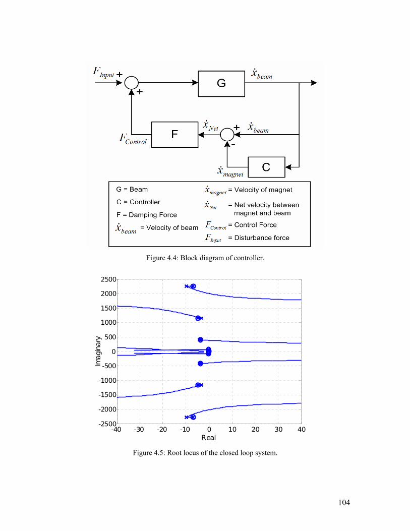
104

Figure 4.4: Block diagram of controller.

-40 -30 -20 -10 0 10 20 30 40-2500

-2000

-1500

-1000

-500

0

500

1000

1500

2000

2500

Real

Imag

inar

y

Figure 4.5: Root locus of the closed loop system.

105

4.3 Experimental Setup of Passive-Active Damper

To validate the predicted response of the passive-active control system experiments were

performed on a cantilever aluminum beam. The dimensions of the beam are shown in Figure 4.6.

For the experiments a neodymium-iron-boron (NdFeB) permanent magnet with radius and length

of 6.35 mm and 12.7 mm, respectively, was used. Other relevant properties of the beam and

magnet are shown in Table 4.1. The analysis of our system required that the eddy currents

generated in the beam be included due to the high conductivity of aluminum.

Fig. 4.6: Schematic showing the dimensions of the beam.

Table 4.1: Physical properties of the beam, conductor and magnet.

Property Value

Young’s modulus of beam 75 GPa

Density of beam 2700 kg/m3

Conductivity of aluminum beam 3.82 x 107 mho/m

Thickness of copper conductor 0.62 mm

Conductivity of copper conductor 5.80 x 107 mho/m

Permanent magnet composition NdFeB 35

Residual magnetic flux of magnet 1.21 kGauss

The passive-active control system functions by sensing the velocity of the beam and the

modifying the position of the permanent magnet such that eddy currents are formed allowing the

vibration of beam to be suppressed without contacting the beam. Two types of disturbances were

applied to the beam and the controller was used to reject them. The first was a continuous

harmonic excitation over a range of frequencies that was generated through a piezoelectric patch

mounted at the root of the beam. The second disturbance was an initial displacement, which was

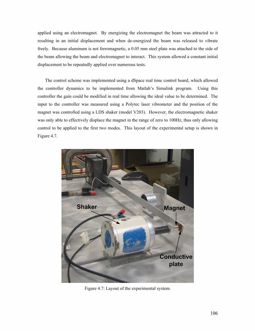
106

applied using an electromagnet. By energizing the electromagnet the beam was attracted to it

resulting in an initial displacement and when de-energized the beam was released to vibrate

freely. Because aluminum is not ferromagnetic, a 0.05 mm steel plate was attached to the side of

the beam allowing the beam and electromagnet to interact. This system allowed a constant initial

displacement to be repeatedly applied over numerous tests.

The control scheme was implemented using a dSpace real time control board, which allowed

the controller dynamics to be implemented from Matlab’s Simulink program. Using this

controller the gain could be modified in real time allowing the ideal value to be determined. The

input to the controller was measured using a Polytec laser vibrometer and the position of the

magnet was controlled using a LDS shaker (model V203). However, the electromagnetic shaker

was only able to effectively displace the magnet in the range of zero to 100Hz, thus only allowing

control to be applied to the first two modes. This layout of the experimental setup is shown in

Figure 4.7.

Figure 4.7: Layout of the experimental system.

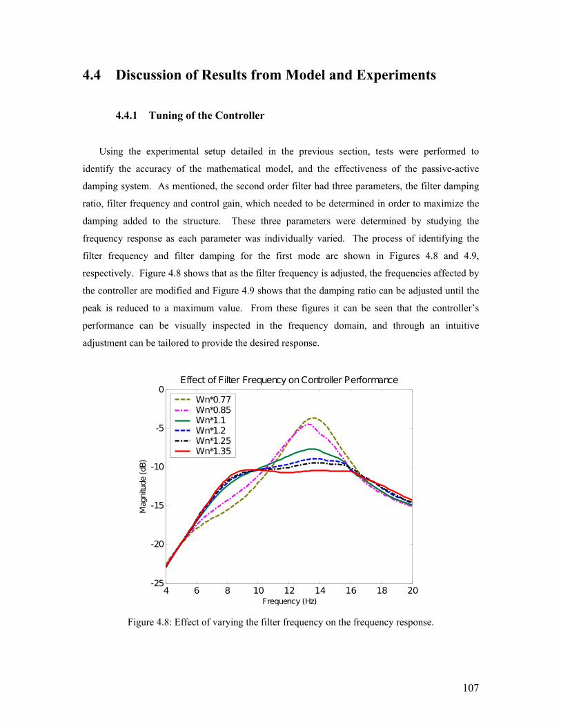
107

4.4 Discussion of Results from Model and Experiments

4.4.1 Tuning of the Controller

Using the experimental setup detailed in the previous section, tests were performed to

identify the accuracy of the mathematical model, and the effectiveness of the passive-active

damping system. As mentioned, the second order filter had three parameters, the filter damping

ratio, filter frequency and control gain, which needed to be determined in order to maximize the

damping added to the structure. These three parameters were determined by studying the

frequency response as each parameter was individually varied. The process of identifying the

filter frequency and filter damping for the first mode are shown in Figures 4.8 and 4.9,

respectively. Figure 4.8 shows that as the filter frequency is adjusted, the frequencies affected by

the controller are modified and Figure 4.9 shows that the damping ratio can be adjusted until the

peak is reduced to a maximum value. From these figures it can be seen that the controller’s

performance can be visually inspected in the frequency domain, and through an intuitive

adjustment can be tailored to provide the desired response.

4 6 8 10 12 14 16 18 20-25

-20

-15

-10

-5

0Effect of Filter Frequency on Controller Performance

Frequency (Hz)

Mag

nitu

de (

dB)

Wn*0.77Wn*0.85Wn*1.1Wn*1.2Wn*1.25Wn*1.35

Figure 4.8: Effect of varying the filter frequency on the frequency response.

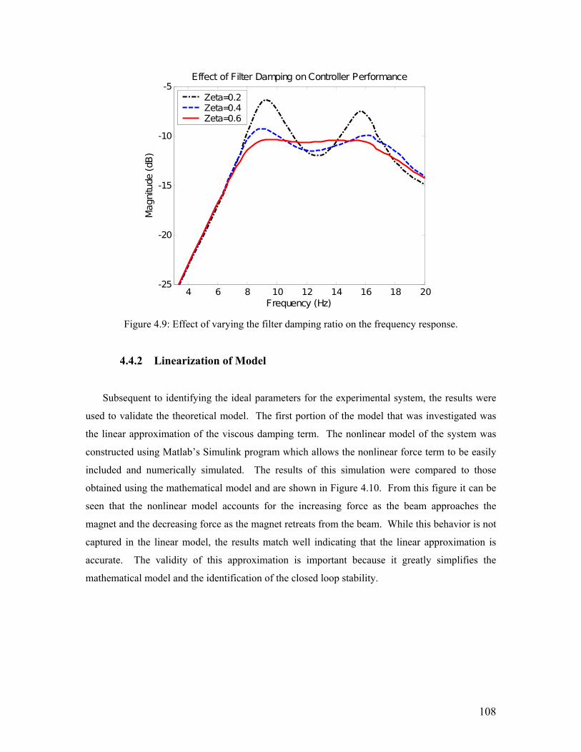
108

4 6 8 10 12 14 16 18 20-25

-20

-15

-10

-5Effect of Filter Damping on Controller Performance

Frequency (Hz)

Magn

itude

(dB

)

Zeta=0.2Zeta=0.4Zeta=0.6

Figure 4.9: Effect of varying the filter damping ratio on the frequency response.

4.4.2 Linearization of Model

Subsequent to identifying the ideal parameters for the experimental system, the results were

used to validate the theoretical model. The first portion of the model that was investigated was

the linear approximation of the viscous damping term. The nonlinear model of the system was

constructed using Matlab’s Simulink program which allows the nonlinear force term to be easily

included and numerically simulated. The results of this simulation were compared to those

obtained using the mathematical model and are shown in Figure 4.10. From this figure it can be

seen that the nonlinear model accounts for the increasing force as the beam approaches the

magnet and the decreasing force as the magnet retreats from the beam. While this behavior is not

captured in the linear model, the results match well indicating that the linear approximation is

accurate. The validity of this approximation is important because it greatly simplifies the

mathematical model and the identification of the closed loop stability.

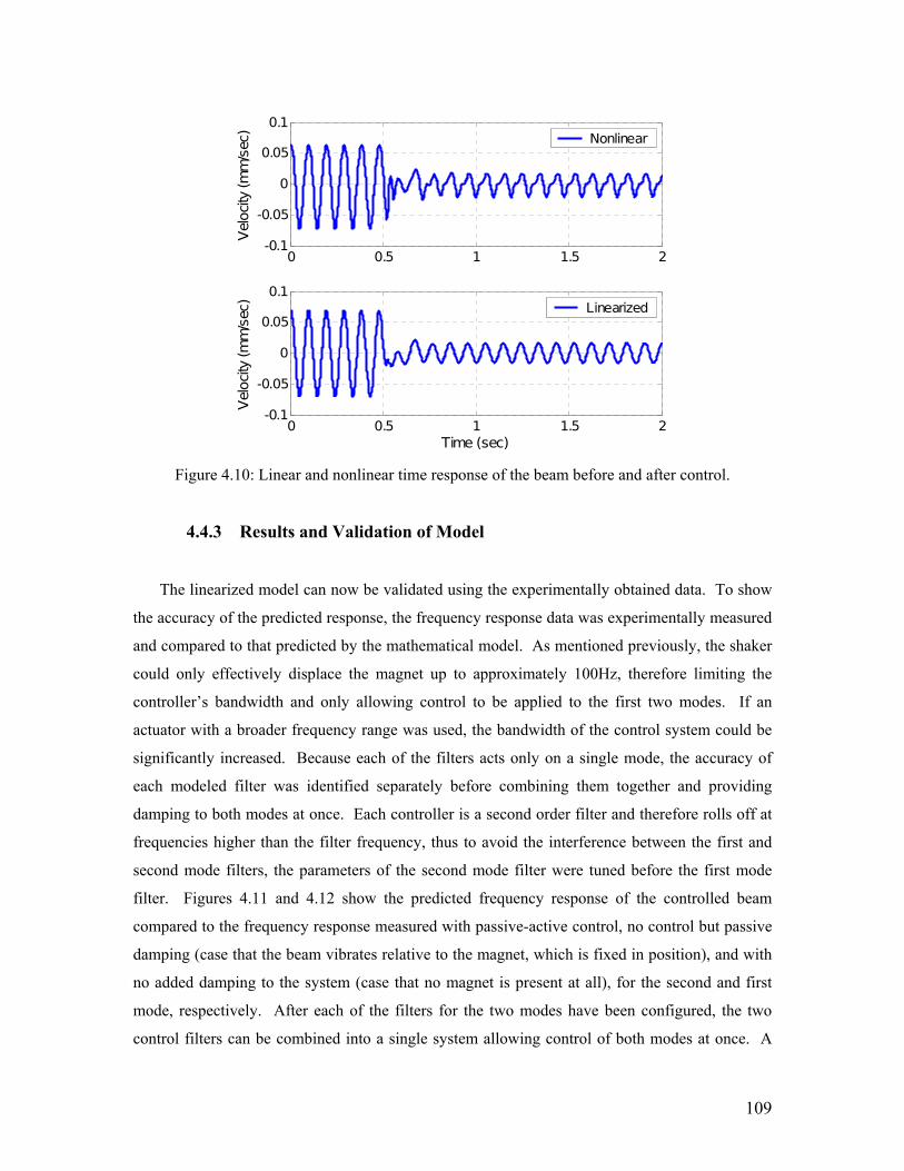
109

0 0.5 1 1.5 2-0.1

-0.05

0

0.05

0.1

Vel

ocity

(mm

/sec

)

0 0.5 1 1.5 2-0.1

-0.05

0

0.05

0.1

Time (sec)

Vel

ocity

(mm

/sec

)

Linearized

Nonlinear

Figure 4.10: Linear and nonlinear time response of the beam before and after control.

4.4.3 Results and Validation of Model

The linearized model can now be validated using the experimentally obtained data. To show

the accuracy of the predicted response, the frequency response data was experimentally measured

and compared to that predicted by the mathematical model. As mentioned previously, the shaker

could only effectively displace the magnet up to approximately 100Hz, therefore limiting the

controller’s bandwidth and only allowing control to be applied to the first two modes. If an

actuator with a broader frequency range was used, the bandwidth of the control system could be

significantly increased. Because each of the filters acts only on a single mode, the accuracy of

each modeled filter was identified separately before combining them together and providing

damping to both modes at once. Each controller is a second order filter and therefore rolls off at

frequencies higher than the filter frequency, thus to avoid the interference between the first and

second mode filters, the parameters of the second mode filter were tuned before the first mode

filter. Figures 4.11 and 4.12 show the predicted frequency response of the controlled beam

compared to the frequency response measured with passive-active control, no control but passive

damping (case that the beam vibrates relative to the magnet, which is fixed in position), and with

no added damping to the system (case that no magnet is present at all), for the second and first

mode, respectively. After each of the filters for the two modes have been configured, the two

control filters can be combined into a single system allowing control of both modes at once. A

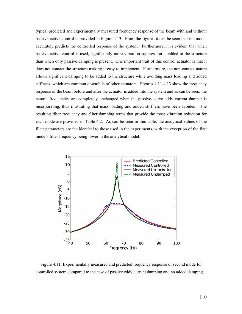
110

typical predicted and experimentally measured frequency response of the beam with and without

passive-active control is provided in Figure 4.13. From the figures it can be seen that the model

accurately predicts the controlled response of the system. Furthermore, it is evident that when

passive-active control is used, significantly more vibration suppression is added to the structure

than when only passive damping is present. One important trait of this control actuator is that it

does not contact the structure making it easy to implement. Furthermore, the non-contact nature

allows significant damping to be added to the structure while avoiding mass loading and added

stiffness, which are common downfalls of other actuators. Figures 4.11-4.13 show the frequency

response of the beam before and after the actuator is added into the system and as can be seen, the

natural frequencies are completely unchanged when the passive-active eddy current damper is

incorporating, thus illustrating that mass loading and added stiffness have been avoided. The

resulting filter frequency and filter damping terms that provide the most vibration reduction for

each mode are provided in Table 4.2. As can be seen in this table, the analytical values of the

filter parameters are the identical to those used in the experiments, with the exception of the first

mode’s filter frequency being lower in the analytical model.

40 50 60 70 80 90 100-35

-30

-25

-20

-15

-10

-5

0

5

10

15

Frequency (Hz)

Magn

itude

(dB

)

P redicted ControlledMeasured ControlledMeasured UncontrolledMeasured Undamped

Figure 4.11: Experimentally measured and predicted frequency response of second mode for

controlled system compared to the case of passive eddy current damping and no added damping.

111

2 4 6 8 10 12 14 16 18 20-45

-40

-35

-30

-25

-20

-15

-10

-5

0

5

Frequency (Hz)

Mag

nitu

de (dB

)

Predicted ControlledMeasured ControlledMeasured UncontrolledMeasured Undamped

Figure 4.12: Experimentally measured and predicted frequency response of first mode for

controlled system compared to the case of passive eddy current damping and no added damping.

10 20 30 40 50 60 70 80 90 100-40

-35

-30

-25

-20

-15

-10

-5

0

5

10

15

Frequency (Hz)

Mag

nitu

de (dB

)

P redicted ControlledMeasured ControlledMeasured Undamped

Figure 4.13: Experimentally measured and predicted frequency response of the beam before and

after passive-active control.

112

Table 4.2: Filter parameters used in experiments and model.

First Mode Second Mode

Experimental Analytical Experimental Analytical

Filter Frequency 1.35 x ω1 1.05 x ω1 0.97 x ω2 0.97 x ω2

Filter Damping Ratio 0.6 0.6 0.125 0.125

Subsequent to identifying the appropriate parameters for each filter and the accuracy of the

mathematical model in the frequency domain, the time response of the system was analyzed.

Using the filter parameters listed in Table 4.2, the beam was excited at its first and second natural

frequency with the magnet located at a fixed position, meaning that passive eddy current damping

was present. Once the beam reached steady state vibration the controller was turned on and the

beam settled to its controlled response. The experimental and predicted results for a continuous

excitation at the beams first natural frequency with the controller turned on at 1.0 sec are shown

in Figure 4.14, while a typical measured and predicted response of the beam excited at the second

natural frequency with the controller turned on at 0.5 seconds are shown in Figure 4.15. As can

be seen from these figures, the controller can quickly suppress the beams vibration. Furthermore,

the amplitude of vibration prior to turning the controller on corresponds to that of passive

damping and once the controller is turned on the amplitude of vibration is reduced by

approximately 79%, thus demonstrating the significant increase in vibration suppression

occurring when the passive-active damping technique is used. Additionally, from these two

figures it is evident that the theoretical model of the passive-active damping system is accurate in

predicting the time response of the controlled beam. However, the model’s accuracy could be

increased by incorporating the nonlinear damping force generated by the eddy current damper,

which is simple to implement in a numerical simulation yet difficult to model analytically.

113

0 0.5 1 1.5 2 2.5-0.1

-0.05

0

0.05

0.1

Time (sec)

Vel

ocity

(m/s

ec)

0 0.5 1 1.5 2 2.5-0.1

-0.05

0

0.05

0.1

Time (sec)

Vel

ocity

(m/s

ec) Measured

Predicted

Figure 4.14: Measured and predicted time response of the beam vibrating at its first bending

mode with the controller turned on at 1.0 second.

0 0.5 1 1.5 2-0.4

-0.2

0

0.2

0.4

Time (sec)

Vel

ocity

(m/s

ec)

0 0.5 1 1.5 2-0.4

-0.2

0

0.2

0.4

Time (sec)

Vel

ocity

(m/s

ec)

Measured

Predicted

Figure 4.15: Measured and predicted time response of the beam vibrating at its second bending

mode with the controller turned on at 0.5 seconds.

Once the performance of the passive-active controller had been demonstrated with a

continuous excitation, its ability to suppress an initial disturbance was investigated. The test was

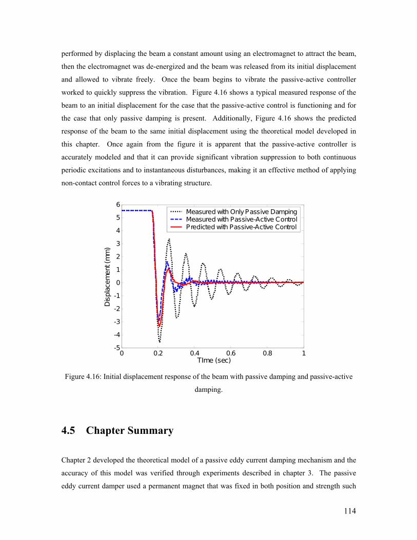
114

performed by displacing the beam a constant amount using an electromagnet to attract the beam,

then the electromagnet was de-energized and the beam was released from its initial displacement

and allowed to vibrate freely. Once the beam begins to vibrate the passive-active controller

worked to quickly suppress the vibration. Figure 4.16 shows a typical measured response of the

beam to an initial displacement for the case that the passive-active control is functioning and for

the case that only passive damping is present. Additionally, Figure 4.16 shows the predicted

response of the beam to the same initial displacement using the theoretical model developed in

this chapter. Once again from the figure it is apparent that the passive-active controller is

accurately modeled and that it can provide significant vibration suppression to both continuous

periodic excitations and to instantaneous disturbances, making it an effective method of applying

non-contact control forces to a vibrating structure.

0 0.2 0.4 0.6 0.8 1-5

-4

-3

-2

-1

0

1

2

3

4

5

6

TIme (sec)

Dis

plac

emen

t (m

m)

Measured with Only Passive DampingMeasured with Passive-Active ControlPredicted with Passive-Active Control

Figure 4.16: Initial displacement response of the beam with passive damping and passive-active

damping.

4.5 Chapter Summary

Chapter 2 developed the theoretical model of a passive eddy current damping mechanism and the

accuracy of this model was verified through experiments described in chapter 3. The passive

eddy current damper used a permanent magnet that was fixed in both position and strength such

115

that the motion of the structure in the magnetic field caused eddy currents to form. As the

currents circulate through the material, they are dissipated by the conductor’s internal resistance

and because a portion of the conductors kinetic energy was used to generate the currents a

damping force results. The density of the eddy currents and the damping force were shown to be

dependent on the velocity of the beam in the magnetic field. In this chapter a passive-active

damping scheme was developed by allowing the position of the magnet to be varied relative to

the beam. The passive component of this new system is the motion of the beam in the static

magnetic field, while an active component is added by controlling the position of the magnet

relative to the beam. By monitoring the beams motion and actively displacing the magnet

accordingly, the net velocity between the permanent magnet and the beam can be controlled such

that the damping applied to the beam can be maximized.

This chapter began by modifying the model developed in chapter 2, such that the motion of

the magnet was included in the damping force. Once the damping force for the passive-active

damping concept was developed, the design of the controller used to actively modify the position

of the magnet was outlined. The controller was chosen to be a second order filter with an input of

the velocity of the structure and an output of the position of the magnet. This choice of controller

input and output was chosen by theoretically and experimentally testing each combination. A

closed loop transfer function of the system was then identified in order to allow the stability of

the system to be shown. Using the root locus method, the closed loop response of a cantilever

beam was shown to be stable for a finite range of gain values. After showing the system’s

stability, the linear approximation used in the theoretical model needed to be verified for

accuracy. The effect of linearization on the model accuracy was identified by comparing the

response of a numerical simulation of the nonlinear system to the predicted response of the linear

system. The results showed that the dynamics were accurately predicted using the linear

assumption.

Once the theoretical model was formulated, an experimental analysis was performed to

demonstrate both the accuracy of model and the performance of the passive-active damper. An

electromagnetic shaker was chosen as the actuator to displace the permanent magnet. However,

the choice of a shaker limited the bandwidth of the controller to 100Hz because the shaker could

not effectively displace the permanent magnet above this frequency. Due to this limited

bandwidth, only the first two modes could be controlled, although if a more sophisticated

displacement actuator were used, higher modes could be targeted. The first step in performing

116

the experimental analysis was to experimentally tune the controller parameters such that it would

provide the most vibration suppression at the resonant frequencies. The resulting values for each

parameter were then compared to those identified from the theoretical model. It was shown that

parameters for each mode matched the model, with the exception of the filter frequency of the

first mode. Once both the model and the experiments were tuned, it was shown that the model

predicted the closed loop response of the beam very well. Furthermore it was demonstrated that

the passive-active controller could reduce the settling time of the passive system by 79%, thus

illustrating its effectiveness as a vibration suppression mechanism.

117

Chapter 5

Active Eddy Current Damping System

5.1 Introduction to the Active Eddy Current Controller

There exist many methods of adding damping to a vibrating structure; however, very few can

function without ever coming into contact with the structure. One such method is eddy current

damping. This magnetic damping scheme functions through the eddy currents that are generated

in a conductive material when it is subjected to a time changing magnetic field. Due to the

circulation of these currents a magnetic field is generated that interacts with the applied field

resulting in a force. In chapters 2-4, passive and passive-active dampers were developed that

caused the formation of eddy currents due to the motion of a conductor in a static magnetic field.

In this chapter, an active damper will be developed that functions by actively modifying the

current flowing in a coil, thus generating a time varying magnetic field. By actively controlling

the strength of the field around the conductor, the eddy currents induced and the resulting

damping force can be controlled.

While the passive eddy current damper developed in chapters 2 and 3, and the passive-active

eddy current damper developed in chapter 4 can provide significant damping to the structure, it is

often desirable to use a completely active system. For instance, in the case of a deployable

satellite it may be necessary to turn the magnetic field off when the satellite is packaged in its

launch configuration, which is not possible when permanent magnets are used. Furthermore, the

use of an active control system allows specific modes of vibration to be targeted and in most

cases more vibration suppression to be achieved. Additionally, in the case of the passive-active

vibration control system, an actuation method was required to displace the magnet relative to the

118

beam, which can be cumbersome and limit the bandwidth of the controller. However, the active

system does not require any additional hardware and can be used to apply control to higher

frequency modes. Lastly, the coil can be made to be very small and lightweight, which is

desirable in space applications.

In previous studies, electromagnets have been located a small distance from a conductive

structure such that the structures motion is in the poling axis, however, none of these studies have

investigated the ability to apply vibration control. For instance, Tani et al. (1990), Morisue

(1990), Tsuboi et al. (1990), Takagi et al. (1992) and Takagi and Tani (1994) have all analyzed

the response of a conducting plate subjected to impulsive magnetic fields. Each of these

researchers has applied upwards of 1000 amps to an electromagnet and predicted the dynamic

response. Additionally, Lee (1996) investigated the stability of electrically conducting beam-

plates when subjected to transverse magnetic fields. The study showed that three stability regions

existed, but never studied the effect of a time changing magnetic field or the ability to use the

system for vibration suppression.

This chapter develops a new active eddy current damper that utilizes an electromagnetic coil

to produce an emf in the beam. First, this chapter will develop the theoretical model of an active

eddy current damper that functions by placing an electromagnetic coil a small distance from a

conductive beam and actively changing the current flowing through the coil. A schematic of the

configuration of the system is shown below in Figure 5.1. As will be shown in the following

sections, the eddy current density will be both a function of the motion of the beam and the time

rate of change of the magnetic field generated by the coil. The beam’s motion will occur due to

its vibration, but the time rate of change of the magnetic flux applied to the beam will be actively

controlled by sensing the beam’s motion and adjusting the current flowing through the coil such

that the damping can be maximized. A feedback controller will be used to modify the current

supplied to the coil in order to control the force applied to the beam. Once the controller has been

developed the system will be numerically simulated and experiments performed to demonstrate

the accuracy of the model. Furthermore, the control system will be shown to be an effective

method of applying vibration control to a vibrating structure.

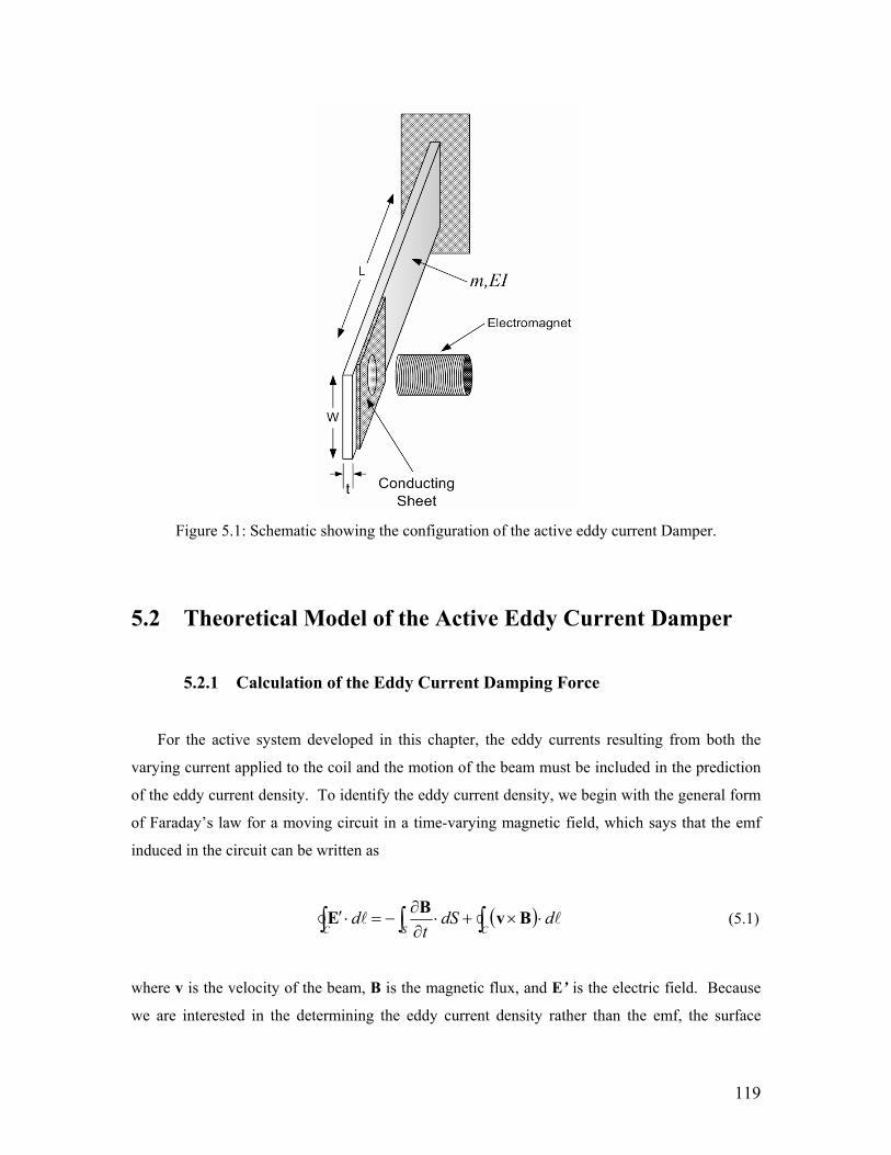
119

Figure 5.1: Schematic showing the configuration of the active eddy current Damper.

5.2 Theoretical Model of the Active Eddy Current Damper

5.2.1 Calculation of the Eddy Current Damping Force

For the active system developed in this chapter, the eddy currents resulting from both the

varying current applied to the coil and the motion of the beam must be included in the prediction

of the eddy current density. To identify the eddy current density, we begin with the general form

of Faraday’s law for a moving circuit in a time-varying magnetic field, which says that the emf

induced in the circuit can be written as

( )∫∫∫ ⋅×+⋅∂∂

−=⋅′CSC

ddSt

d BvBE (5.1)

where v is the velocity of the beam, B is the magnetic flux, and E’ is the electric field. Because

we are interested in the determining the eddy current density rather than the emf, the surface

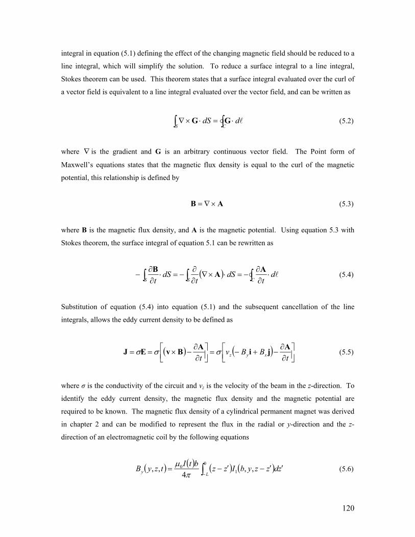
120

integral in equation (5.1) defining the effect of the changing magnetic field should be reduced to a

line integral, which will simplify the solution. To reduce a surface integral to a line integral,

Stokes theorem can be used. This theorem states that a surface integral evaluated over the curl of

a vector field is equivalent to a line integral evaluated over the vector field, and can be written as

∫ ∫ ⋅=⋅×∇S C

ddS GG (5.2)

where ∇ is the gradient and G is an arbitrary continuous vector field. The Point form of

Maxwell’s equations states that the magnetic flux density is equal to the curl of the magnetic

potential, this relationship is defined by

AB ×∇= (5.3)

where B is the magnetic flux density, and A is the magnetic potential. Using equation 5.3 with

Stokes theorem, the surface integral of equation 5.1 can be rewritten as

( ) ∫∫∫ ⋅∂∂

−=⋅×∇∂∂

−=⋅∂∂

−CSS

dt

dSt

dSt

AAB (5.4)

Substitution of equation (5.4) into equation (5.1) and the subsequent cancellation of the line

integrals, allows the eddy current density to be defined as

( ) ( ) ⎥⎦⎤

⎢⎣⎡

∂∂

−+−=⎥⎦⎤

⎢⎣⎡

∂∂

−×==t

BBvt xyz

AjiABvEJ σσσ (5.5)

where σ is the conductivity of the circuit and vz is the velocity of the beam in the z-direction. To

identify the eddy current density, the magnetic flux density and the magnetic potential are

required to be known. The magnetic flux density of a cylindrical permanent magnet was derived

in chapter 2 and can be modified to represent the flux in the radial or y-direction and the z-

direction of an electromagnetic coil by the following equations

( ) ( ) ( ) ( )∫− ′′−′−=0

10 ,,4

,,Ly zdzzybIzzbtItzyB

πµ

(5.6)

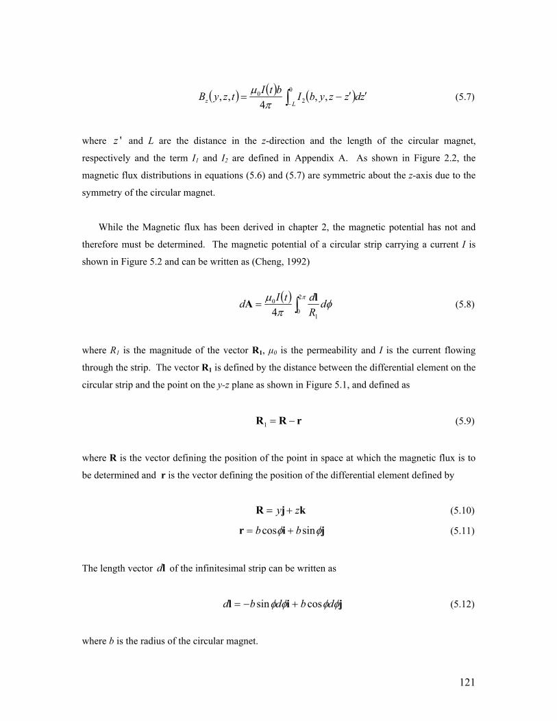
121

( ) ( ) ( )∫− ′′−=0

20 ,,4

,,Lz zdzzybIbtItzyB

πµ

(5.7)

where 'z and L are the distance in the z-direction and the length of the circular magnet,

respectively and the term I1 and I2 are defined in Appendix A. As shown in Figure 2.2, the

magnetic flux distributions in equations (5.6) and (5.7) are symmetric about the z-axis due to the

symmetry of the circular magnet.

While the Magnetic flux has been derived in chapter 2, the magnetic potential has not and

therefore must be determined. The magnetic potential of a circular strip carrying a current I is

shown in Figure 5.2 and can be written as (Cheng, 1992)

( )∫=

πφ

πµ 2

01

0

4d

RdtId lA (5.8)

where R1 is the magnitude of the vector R1, µ0 is the permeability and I is the current flowing

through the strip. The vector R1 is defined by the distance between the differential element on the

circular strip and the point on the y-z plane as shown in Figure 5.1, and defined as

rRR −=1 (5.9)

where R is the vector defining the position of the point in space at which the magnetic flux is to

be determined and r is the vector defining the position of the differential element defined by

kjR zy += (5.10)

jir φφ sincos bb += (5.11)

The length vector dl of the infinitesimal strip can be written as

jil φφφφ dbdbd cossin +−= (5.12)

where b is the radius of the circular magnet.

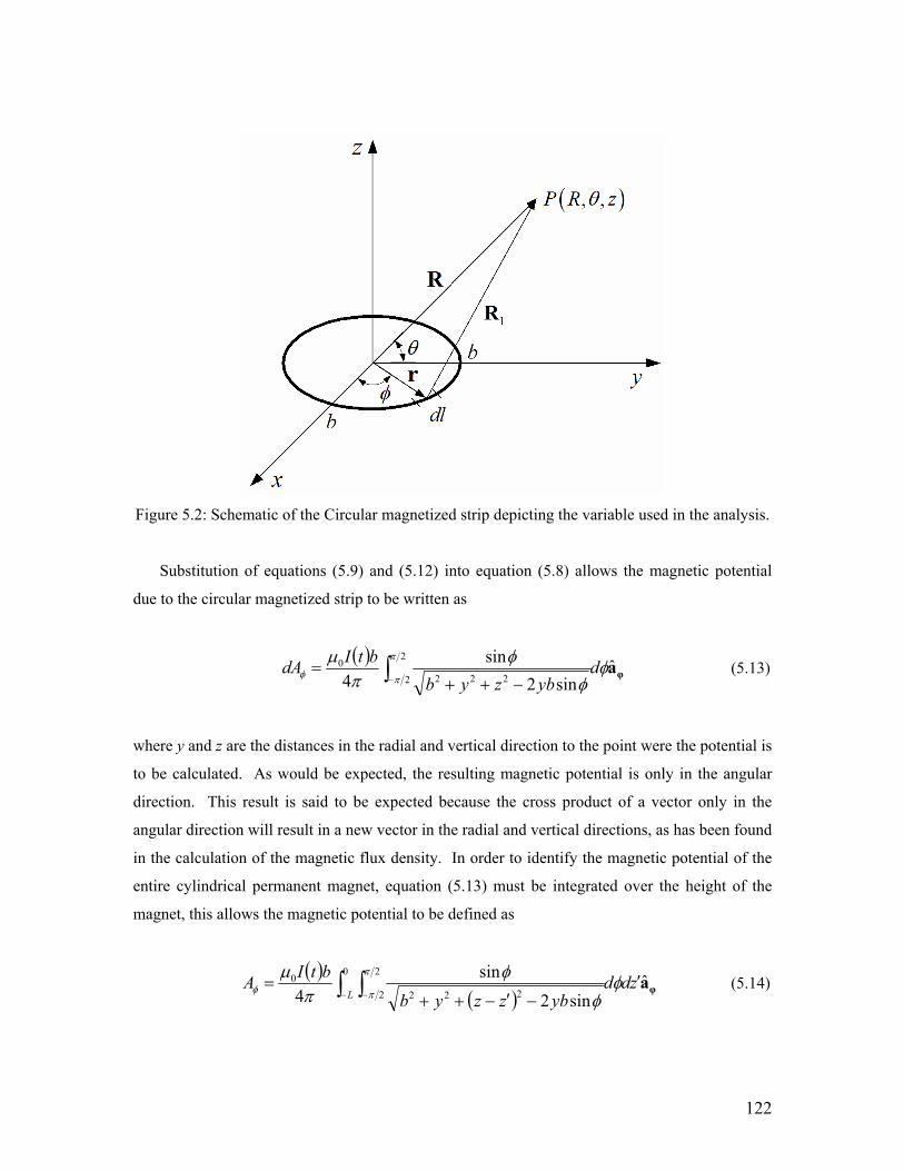
122

Figure 5.2: Schematic of the Circular magnetized strip depicting the variable used in the analysis.

Substitution of equations (5.9) and (5.12) into equation (5.8) allows the magnetic potential

due to the circular magnetized strip to be written as

( )φa

sin2sin

42

2 2220 φ

φφ

πµ π

πφ dybzyb

btIdA ∫− −++= (5.13)

where y and z are the distances in the radial and vertical direction to the point were the potential is

to be calculated. As would be expected, the resulting magnetic potential is only in the angular

direction. This result is said to be expected because the cross product of a vector only in the

angular direction will result in a new vector in the radial and vertical directions, as has been found

in the calculation of the magnetic flux density. In order to identify the magnetic potential of the

entire cylindrical permanent magnet, equation (5.13) must be integrated over the height of the

magnet, this allows the magnetic potential to be defined as

( )( ) φa

sin2

sin4

0 2

2 2220 ∫ ∫− −

′−′−++

=L

zddybzzyb

btIA φφ

φπ

µ π

πφ (5.14)

123

where z’ is the differential height of the magnet. Equation (5.14) can now be used along with

equation (5.6) to calculate the eddy current density of equation (5.5). Once the eddy current

density is known the damping force can be determined by

( ) ( )

( ) ( ) z

z

a

a

BJF

ˆ,,2

ˆ,,

0

2

0

2

0 0

22

0 0

⎥⎦

⎤⎢⎣

⎡−

∂∂

=

⎥⎦

⎤⎢⎣

⎡−

∂∂

=

×=

∫∫

∫ ∫∫ ∫

∫

cc

cc

r

gy

r

gy

g

r

y

r

gy

V

dylyyBvdylyBt

Ay

dydlyyBvdydlyBt

Ay

dV

φ

ππ φ

πσδ

φφσδ (5.15)

where δ and v are the thickness and the vertical velocity of the conducting sheet, respectively, rc

is the equivalent radius of the conductor that preserves its surface area and lg is the distance

between the conducting sheet and the bottom of magnet as was shown in Figure 2.2. When the

damping force is included into the equation of motion of the beam, it is split into two terms, one

defining the force due to a transformer emf and the second due to a motional emf. Equation

(5.15) contains two integrals, the first defines the transformer emf, or the force due to the time

changing magnetic field and the second integral defines the motional emf, or the eddy current

damping force due to the beam’s velocity in the magnetic field. The transformer force must be

included as an external force and the motional force can be included as a damping term due to its

dependence on the velocity of the beam. The integration of equations (5.6), (5.14) and (5.15)

cannot be solved for analytically because they result in a series of elliptical integrals and therefore

a numerical integration method must be used to obtain the damping force in equation (5.15). This

damping force can now be incorporated into the dynamics of the beam and the response can be

determined. However, in looking at equation (5.15) it can be seen that the eddy currents due to

both the motional and transformer emf are very nonlinear. For this reason the dynamics response

of the the system response will be numerically simulated in MATLAB’s Simulink program.

The force generated by actively controlling the strength of the magnetic field, results in an

interesting effect; the frequency of the force applied to the beam is twice the frequency of the

current applied to the coil. This effect is due to the trigonometric identity that states the product

of a sine and cosine wave results in a sine wave at twice the frequency of two waves. This

identity appears in the first integral in equation (5.15) defining the transformer portion of the eddy

current damping force as the product of the derivative of the magnetic potential and the magnetic

124

flux density. It may not be immediately apparent that this effect occurs until it is realized that the

magnetic flux density and magnetic potential are both a function of the time dependent current

applied to the electromagnet. This force doubling effect has serious consequences that affect the

design and performance of the active eddy current control system, and will be discussed in

section 5.2.3.

5.2.2 Inclusion of Active Damping in Beam Equation

The response of the beam and the eddy current damper can be defined in a very similar manor

as was done in chapter 4. The equation of motion for a beam was derived in chapter 2 and can be

written as follows

( ) ( ) ( ) ( ) ( ) ( ) ( )∫ ∑=

+=++L p

iii xtFdxxtxftrtrtr

01

, φφKCM (5.16)

where the mass matrix M, the damping matrix C, and the stiffness matrix K are defined by

( ) ( ) ( )∫==L T

ij dxxxxm0

φφρM (5.17)

( ) ( ) ( )∫ ′′′′==L T

ij dxxxxEIk0

φφK (5.18)

( ) ( )∫==L

bT

ij dxxcxc0

φφC (5.19)

where E is the modulus of elasticity, I is the beam’s moment of inertia, ρ is the area density of the

beam, cb is the beam’s damping coefficient, f(x,t) are distributed forces, Fi are concentrated

forces, and ( )xφ is the assumed mode shape of the beam. The equation of motion for the passive

and passive-active cases differs from the active damper, because there are now two separate eddy

current force terms. As mentioned in the previous section, one term is modeled as a concentrated

external force, while the other is modeled as a viscous damping force. The eddy current force due

to the transformer emf is included as a concentrated force and can be written as

( ) ( ) ( )e

r

yT xdyBt

AyFxtF c φπσδφ φ

⎥⎦

⎤⎢⎣

⎡∂∂

== ∫011 2 (5.20)

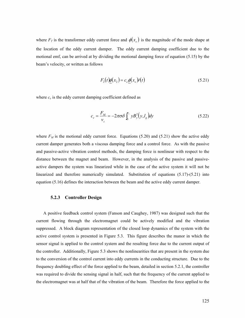
125

where FT is the transformer eddy current force and ( )exφ is the magnitude of the mode shape at

the location of the eddy current damper. The eddy current damping coefficient due to the

motional emf, can be arrived at by dividing the motional damping force of equation (5.15) by the

beam’s velocity, or written as follows

( ) ( ) ( ) ( )trxcxtF eeφφ =22 (5.21)

where ce is the eddy current damping coefficient defined as

( )∫−==cr

gyz

Me dylyyB

vFc

0

2 ,2πσδ (5.22)

where FM is the motional eddy current force. Equations (5.20) and (5.21) show the active eddy

current damper generates both a viscous damping force and a control force. As with the passive

and passive-active vibration control methods, the damping force is nonlinear with respect to the

distance between the magnet and beam. However, in the analysis of the passive and passive-

active dampers the system was linearized while in the case of the active system it will not be

linearized and therefore numerically simulated. Substitution of equations (5.17)-(5.21) into

equation (5.16) defines the interaction between the beam and the active eddy current damper.

5.2.3 Controller Design

A positive feedback control system (Fanson and Caughey, 1987) was designed such that the

current flowing through the electromagnet could be actively modified and the vibration

suppressed. A block diagram representation of the closed loop dynamics of the system with the

active control system is presented in Figure 5.3. This figure describes the manor in which the

sensor signal is applied to the control system and the resulting force due to the current output of

the controller. Additionally, Figure 5.3 shows the nonlinearities that are present in the system due

to the conversion of the control current into eddy currents in the conducting structure. Due to the

frequency doubling effect of the force applied to the beam, detailed in section 5.2.1, the controller

was required to divide the sensing signal in half, such that the frequency of the current applied to

the electromagnet was at half that of the vibration of the beam. Therefore the force applied to the

126

beam would be at the same frequency as its vibration. The equation used to divide the force is

half is as follows

( )∫=⎟⎠⎞

⎜⎝⎛

tdtωω sin

21sin (5.23)

were ω is the frequency of the harmonic signal. This equation is applied to the output of the

control filters which were designed for each mode. The feedback controller is a second order

filter with three parameters chosen to provide the greatest vibration suppression to the frequency

response. Two separate filter designs were used and are defined as

22

2

2 fff

f

ssK

ωωζω

++ (5.24)

22

22

2 fff

f

ssK

ωωζω

++ (5.25)

where K is the controller gain, ωf is the filter frequency and ζf is the filter damping ratio. The

filter defined in equation (5.24) was used to apply control to all modes but the second mode,

which was controlled using the filter defined in equation (5.25). Both compensators defined in

equations (5.24) and (5.25) contain an extra zero in the numerator to account for the integration

used in equation (5.23) that is required to reduce the frequency of the sensing signal by half. The

filter of equation (5.25) contains an additional zero to account for a phase shift that occurs after

the natural frequency in the closed loop response of the beam. The closed loop response of the

beam’s second mode with the filter of equation (5.24) and equation (5.25) can be seen in the

frequency response of Figure 5.4. This phase shift can be seen as a drop in the phase after the

natural frequency. The phase shift leads to an amplification of the response above the natural

frequency. This variation is caused by the relationship between the current applied to the coil and

the magnetic field generated. The effect of the coil was not immediately realized and results

showing the predicted response of the system before the coil dynamics were identified will be

presented first, followed by the results after the relation is included into the simulation.

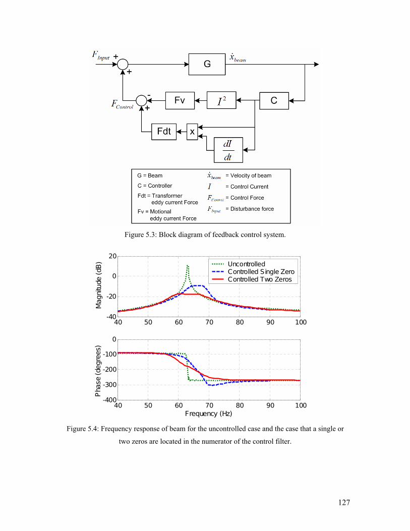
127

Figure 5.3: Block diagram of feedback control system.

40 50 60 70 80 90 100-40

-20

0

20

Mag

nitu

de (

dB)

40 50 60 70 80 90 100-400

-300

-200

-100

0

Frequency (Hz)

Pha

se (

degr

ees)

UncontrolledControlled Single ZeroControlled Two Zeros

Figure 5.4: Frequency response of beam for the uncontrolled case and the case that a single or

two zeros are located in the numerator of the control filter.

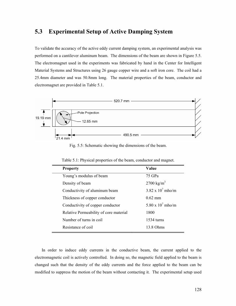
128

5.3 Experimental Setup of Active Damping System

To validate the accuracy of the active eddy current damping system, an experimental analysis was

performed on a cantilever aluminum beam. The dimensions of the beam are shown in Figure 5.5.

The electromagnet used in the experiments was fabricated by hand in the Center for Intelligent

Material Systems and Structures using 26 gauge copper wire and a soft iron core. The coil had a

25.4mm diameter and was 50.8mm long. The material properties of the beam, conductor and

electromagnet are provided in Table 5.1.

Fig. 5.5: Schematic showing the dimensions of the beam.

Table 5.1: Physical properties of the beam, conductor and magnet.

Property Value

Young’s modulus of beam 75 GPa

Density of beam 2700 kg/m3

Conductivity of aluminum beam 3.82 x 107 mho/m

Thickness of copper conductor 0.62 mm

Conductivity of copper conductor 5.80 x 107 mho/m

Relative Permeability of core material 1800

Number of turns in coil 1534 turns

Resistance of coil 13.8 Ohms

In order to induce eddy currents in the conductive beam, the current applied to the

electromagnetic coil is actively controlled. In doing so, the magnetic field applied to the beam is

changed such that the density of the eddy currents and the force applied to the beam can be

modified to suppress the motion of the beam without contacting it. The experimental setup used

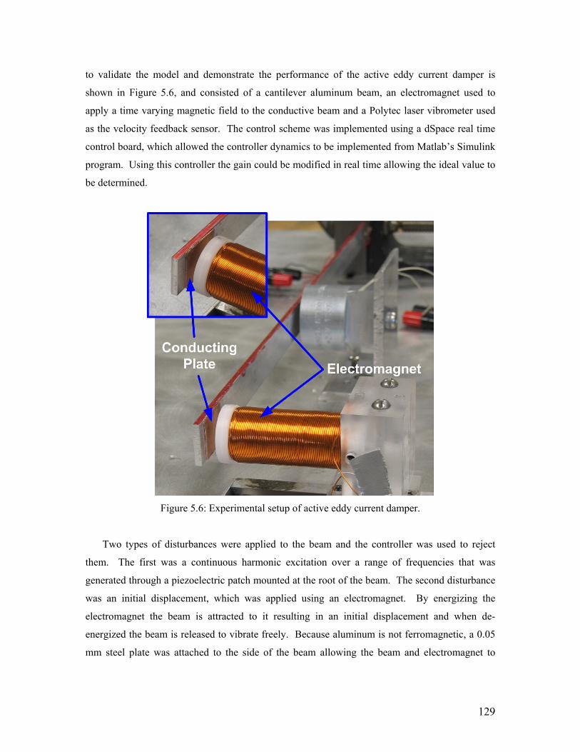
129

to validate the model and demonstrate the performance of the active eddy current damper is

shown in Figure 5.6, and consisted of a cantilever aluminum beam, an electromagnet used to

apply a time varying magnetic field to the conductive beam and a Polytec laser vibrometer used

as the velocity feedback sensor. The control scheme was implemented using a dSpace real time

control board, which allowed the controller dynamics to be implemented from Matlab’s Simulink

program. Using this controller the gain could be modified in real time allowing the ideal value to

be determined.

Figure 5.6: Experimental setup of active eddy current damper.

Two types of disturbances were applied to the beam and the controller was used to reject

them. The first was a continuous harmonic excitation over a range of frequencies that was

generated through a piezoelectric patch mounted at the root of the beam. The second disturbance

was an initial displacement, which was applied using an electromagnet. By energizing the

electromagnet the beam is attracted to it resulting in an initial displacement and when de-

energized the beam is released to vibrate freely. Because aluminum is not ferromagnetic, a 0.05

mm steel plate was attached to the side of the beam allowing the beam and electromagnet to

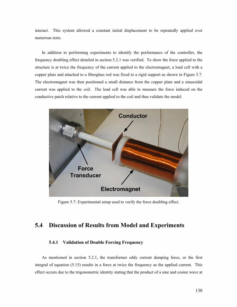
130

interact. This system allowed a constant initial displacement to be repeatedly applied over

numerous tests.

In addition to performing experiments to identify the performance of the controller, the

frequency doubling effect detailed in section 5.2.1 was verified. To show the force applied to the

structure is at twice the frequency of the current applied to the electromagnet, a load cell with a

copper plate and attached to a fiberglass rod was fixed to a rigid support as shown in Figure 5.7.

The electromagnet was then positioned a small distance from the copper plate and a sinusoidal

current was applied to the coil. The load cell was able to measure the force induced on the

conductive patch relative to the current applied to the coil and thus validate the model.

Figure 5.7: Experimental setup used to verify the force doubling effect.

5.4 Discussion of Results from Model and Experiments

5.4.1 Validation of Double Forcing Frequency

As mentioned in section 5.2.1, the transformer eddy current damping force, or the first

integral of equation (5.15) results in a force at twice the frequency as the applied current. This

effect occurs due to the trigonometric identity stating that the product of a sine and cosine wave at

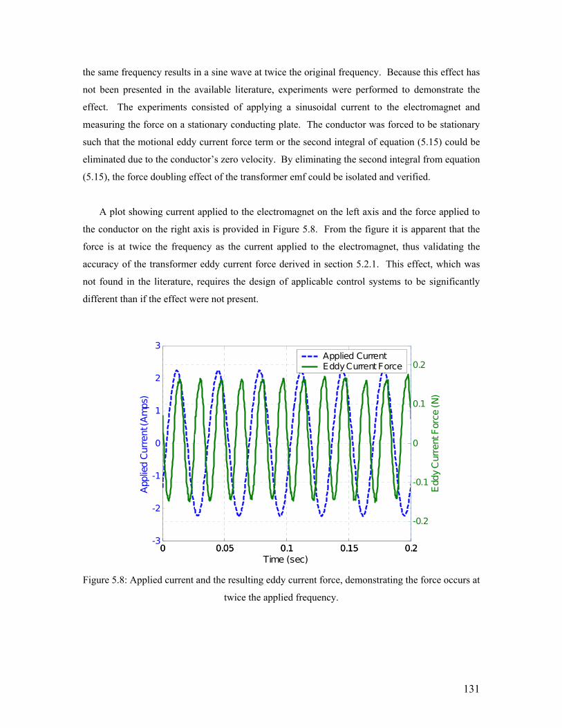
131

the same frequency results in a sine wave at twice the original frequency. Because this effect has

not been presented in the available literature, experiments were performed to demonstrate the

effect. The experiments consisted of applying a sinusoidal current to the electromagnet and

measuring the force on a stationary conducting plate. The conductor was forced to be stationary

such that the motional eddy current force term or the second integral of equation (5.15) could be

eliminated due to the conductor’s zero velocity. By eliminating the second integral from equation

(5.15), the force doubling effect of the transformer emf could be isolated and verified.

A plot showing current applied to the electromagnet on the left axis and the force applied to

the conductor on the right axis is provided in Figure 5.8. From the figure it is apparent that the

force is at twice the frequency as the current applied to the electromagnet, thus validating the

accuracy of the transformer eddy current force derived in section 5.2.1. This effect, which was

not found in the literature, requires the design of applicable control systems to be significantly

different than if the effect were not present.

0 0.05 0.1 0.15 0.2-3

-2

-1

0

1

2

3

App

lied

Cur

rent

(A

mps)

Time (sec)0 0.05 0.1 0.15 0.2

-0.2

-0.1

0

0.1

0.2

Edd

y C

urre

nt F

orce

(N

)

Applied CurrentEddy Current Force

Figure 5.8: Applied current and the resulting eddy current force, demonstrating the force occurs at

twice the applied frequency.

132

5.4.2 Tuning of the Controller

Once the controllers detailed in section 5.2.3 were designed, the appropriate filter properties

had to be identified. This process was detailed in section 4.3.1 of chapter 4 and consists of

observing the closed loop frequency response of the system and modifying the parameters to

achieve maximum damping. This process was first performed in the numerical simulation to

identify the predicted parameter and then these parameters were applied to the experiments and

retuned to obtain the variation in filter parameters. The resulting parameters and the performance

of the active control system will be provided in the subsequent section. Once the filter had been

tuned it could be effectively used to suppress the vibration of the beam.

5.4.3 Results and Validation of Model

Once the filters have been tuned to apply the maximum control to each targeted frequency,

the performance of the new active eddy current control system and the accuracy of the modeling

techniques developed in this chapter can be demonstrated through a comparison of experimental

and analytical results. Each controller is a second order filter that applies vibration suppression to

a narrow band of frequencies, typically located around one of the system’s natural frequencies;

therefore if multiple modes of vibration are to be controlled, each filter must be designed

separately. As mentioned in chapter 4, the second order filter rolls off at frequencies higher than

the filter frequency, thus allowing each filter to have little effect on higher modes but can lead to

spillover and destabilization of the lower frequencies. To avoid these negative effects, it is

standard that the higher mode controllers be designed first. To demonstrate the accuracy of the

theoretical model, both the frequency response and the time response of the system will be

experimentally measured and predicted through a numerical simulation.

Because tuning of the controller can be most easily seen in the frequency response, we will

begin by comparing the predicted and measured frequency response of the closed loop system.

Typically before multiple modes are controlled it is advantageous to apply control to each mode

separately, thus identifying trends in the filter parameters and modes that may have little

controllability, before compiling the entire group of filters together and trying to tune them.

Therefore, in the following plots between the predicted and measured frequency response, the

133

predicted response was tuned first to obtain the rough location of the experimental parameter

allowing the experimental filters to be quickly adjusted.

First, the frequency response of the active control system when applied to a single mode will

be predicted and compared to the experimental data. Figures 5.9 and 5.10 provide the measured

and predicted closed loop frequency response of the second and first mode compared to the

uncontrolled response of the beam. From these two figures it is evident that the active eddy

current control system can effectively apply vibration suppression to the cantilever beam. The

control system provides the second mode, shown in Figure 5.9, with approximately 29dB

(approximately 96.6% suppression) reduction in vibration and the first mode, shown in Figure

5.11, with approximately 30.5dB (greater than 97% suppression) reduction in vibration. These

results indicate the effectiveness of this new non-contact actuation system. Once the system was

demonstrated to be effective at each frequency, multiple filters were used together in order to

target several frequencies at once. One experiment performed, looked at applying control to the

first three modes of the cantilever beam and compared the measured frequency response to the

response predicted in the numerical simulation of the theoretical model. The three mode

controlled frequency response function for the case that the filter parameters are experimentally

tuned and the case that the filter parameters are tuned in the numerical simulation are compared to

the uncontrolled frequency response in Figure 5.11. The filter parameters used to apply control to

each mode for the theoretical and experimental cases are provided in Table 5.2. This experiment

was performed by tuning the controller parameters in the numerical simulation, then taking the

predicted parameters and applying them to the experimental system. While the predicted and

measured values do not lie directly upon each other, the two tuned responses do fall on top of

each other indicating that the numerical simulation provides a reasonably good prediction of the

maximum vibration suppression that can be achieved. The parameters that provide the maximum

vibration reduction in the theoretical model do not exactly match the experimentally tuned values

for reasons that will be discussed in the subsequent section.

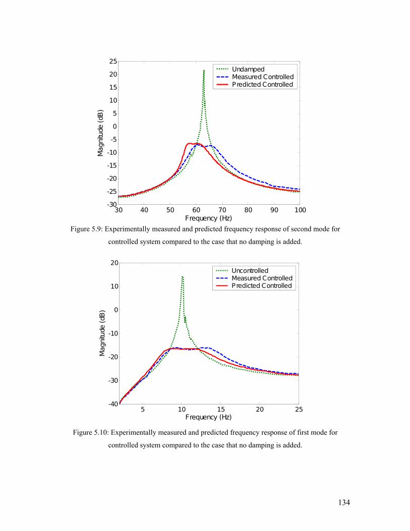
134

30 40 50 60 70 80 90 100-30

-25

-20

-15

-10

-5

0

5

10

15

20

25

Frequency (Hz)

Mag

nitu

de (dB

)

UndampedMeasured ControlledPredicted Controlled

Figure 5.9: Experimentally measured and predicted frequency response of second mode for

controlled system compared to the case that no damping is added.

5 10 15 20 25-40

-30

-20

-10

0

10

20

Frequency (Hz)

Mag

nitu

de (dB

)

UncontrolledMeasured ControlledPredicted Controlled

Figure 5.10: Experimentally measured and predicted frequency response of first mode for

controlled system compared to the case that no damping is added.

135

0 50 100 150 200

-30

-20

-10

0

10

20

30

Frequency (Hz)

Mag

nitu

de (dB

)

UncontrolledMeasured ControlledPredicted Controlled

Figure 5.11: Measured and predicted controlled response of the cantilever beam’s first three

bending modes compared to the uncontrolled case.

Table 5.2: Filter parameters used in the experiments and theory.

First Mode Second Mode Third Mode

Measured Predicted Measured Predicted Measured Predicted

Filter Frequency 1.37xω1 1.06xω1 0. 987xω2 0.875xω2 0.935xω3 0.985xω3

Filter Damping 0.34 0.4 0.1 0.065 0.07 0.07

Filter Gain -4 -25 -0.005 -0.0055 -4 -1.275

Identification of Model Inaccuracy Source

One occurrence that shows some of the system’s dynamics are not modeled is the shift in the

peak of the predicted controlled natural frequency, which can be seen in both Figures 5.9 and

5.11. This type of magnitude shift was also noticed in the experimental study and is documented

in section 5.2.3 and Figure 5.4. However, the shift was evident in the experiments when the

second mode’s filter only had a single free derivative and is present in the theoretical case when

the system has two free derivatives, but not a single. This difference made it apparent that a

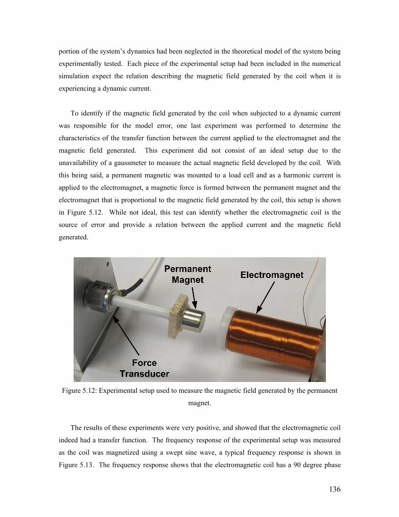
136

portion of the system’s dynamics had been neglected in the theoretical model of the system being

experimentally tested. Each piece of the experimental setup had been included in the numerical

simulation expect the relation describing the magnetic field generated by the coil when it is

experiencing a dynamic current.

To identify if the magnetic field generated by the coil when subjected to a dynamic current

was responsible for the model error, one last experiment was performed to determine the

characteristics of the transfer function between the current applied to the electromagnet and the

magnetic field generated. This experiment did not consist of an ideal setup due to the

unavailability of a gaussmeter to measure the actual magnetic field developed by the coil. With

this being said, a permanent magnetic was mounted to a load cell and as a harmonic current is

applied to the electromagnet, a magnetic force is formed between the permanent magnet and the

electromagnet that is proportional to the magnetic field generated by the coil, this setup is shown

in Figure 5.12. While not ideal, this test can identify whether the electromagnetic coil is the

source of error and provide a relation between the applied current and the magnetic field

generated.

Figure 5.12: Experimental setup used to measure the magnetic field generated by the permanent

magnet.

The results of these experiments were very positive, and showed that the electromagnetic coil

indeed had a transfer function. The frequency response of the experimental setup was measured

as the coil was magnetized using a swept sine wave, a typical frequency response is shown in

Figure 5.13. The frequency response shows that the electromagnetic coil has a 90 degree phase

137

shift, and has a break frequency at 15Hz, after witch the magnetic force generated has 20dB

attenuation per decade as the frequency is increased. These two characteristics of the frequency

response can be modeled as a single pole at 15Hz. Using this result, the dynamics of the

electromagnetic coil can be included in the numerical simulation and the dynamics of the

cantilever beam can be recalculated. However, the measured response shown in Figure 5.13

begins to have other dynamics at approximately 210Hz, which is almost the exact frequency at

which the third mode of the system occurs. Beyond this frequency the magnetic field generated

by the electromagnet cannot be accurately measured without a gaussmeter, thus interfering with

the ability to model the electromagnet at higher frequencies. As was shown previously, the

dynamics of the electromagnetic coil lead to inaccuracies in the model, thus to avoid these

inaccuracies only the first two modes of the structure that lie in the accurate range of the

measured field will be modeled. The frequency responses predicted by the theoretical model

when the dynamics of the electromagnetic coil are included in the simulation, compared to the

measured frequency response, are shown in Figure 5.14. As can be seen in the figure, the model

now more accurately predicts the frequency response and the second mode no longer has a shift

in the magnitude of the controlled response. The filter parameters used to apply control to each

mode for the theoretical model that includes the magnets dynamics, and experiments are provided

in Table 5.3. From this table, it can be seen that all tuned parameters used in the theory are now

almost identical to those used in the experiments. These results indicate that the source of error in

the previously calculated frequency response was due to the phase shift between the current

applied to the coil and the resulting magnetic field.

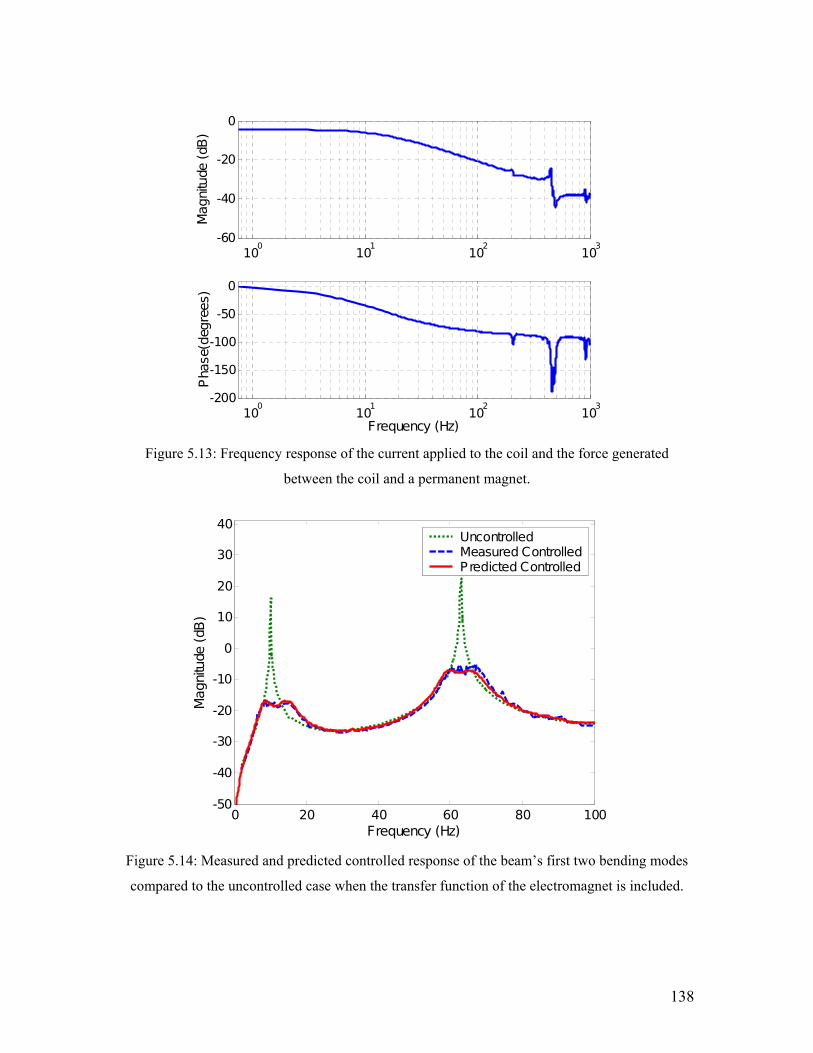
138

100

101

102

103

-60

-40

-20

0

Mag

nitu

de (dB

)

100

101

102

103

-200

-150

-100

-50

0

Frequency (Hz)

Pha

se(d

egre

es)

Figure 5.13: Frequency response of the current applied to the coil and the force generated

between the coil and a permanent magnet.

0 20 40 60 80 100-50

-40

-30

-20

-10

0

10

20

30

40

Frequency (Hz)

Mag

nitu

de (dB

)

UncontrolledMeasured ControlledPredicted Controlled

Figure 5.14: Measured and predicted controlled response of the beam’s first two bending modes

compared to the uncontrolled case when the transfer function of the electromagnet is included.

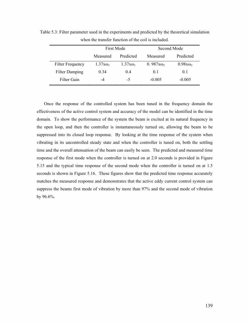
139

Table 5.3: Filter parameter used in the experiments and predicted by the theoretical simulation

when the transfer function of the coil is included.

First Mode Second Mode

Measured Predicted Measured Predicted

Filter Frequency 1.37xω1 1.37xω1 0. 987xω2 0.98xω2

Filter Damping 0.34 0.4 0.1 0.1

Filter Gain -4 -5 -0.005 -0.005

Once the response of the controlled system has been tuned in the frequency domain the

effectiveness of the active control system and accuracy of the model can be identified in the time

domain. To show the performance of the system the beam is excited at its natural frequency in

the open loop, and then the controller is instantaneously turned on, allowing the beam to be

suppressed into its closed loop response. By looking at the time response of the system when

vibrating in its uncontrolled steady state and when the controller is tuned on, both the settling

time and the overall attenuation of the beam can easily be seen. The predicted and measured time

response of the first mode when the controller is turned on at 2.0 seconds is provided in Figure

5.15 and the typical time response of the second mode when the controller is turned on at 1.5

seconds is shown in Figure 5.16. These figures show that the predicted time response accurately

matches the measured response and demonstrates that the active eddy current control system can

suppress the beams first mode of vibration by more than 97% and the second mode of vibration

by 96.6%.

140

0 0.5 1 1.5 2 2.5 3 3.5 4-0.04

-0.02

0

0.02

0.04

Vel

ocity

(m/s

ec)

0 0.5 1 1.5 2 2.5 3 3.5 4-0.04

-0.02

0

0.02

0.04

Time (sec)

Vel

ocity

(m/s

ec) Measured

Predicted

Figure 5.15: Measured and predicted time response of the beam excited at its first bending mode

with the controller turned on at 2.0 seconds.

0 0.5 1 1.5 2 2.5 3-0.2

-0.1

0

0.1

0.2

Vel

ocity

(m

/sec

)

0 0.5 1 1.5 2 2.5 3-0.2

-0.1

0

0.1

0.2

Time (sec)

Vel

ocity

(m

/sec

) Measured

Predicted

Figure 5.16: Measured and predicted time response of the beam excited at its second bending

mode with the controller turned on at 1.5 seconds.

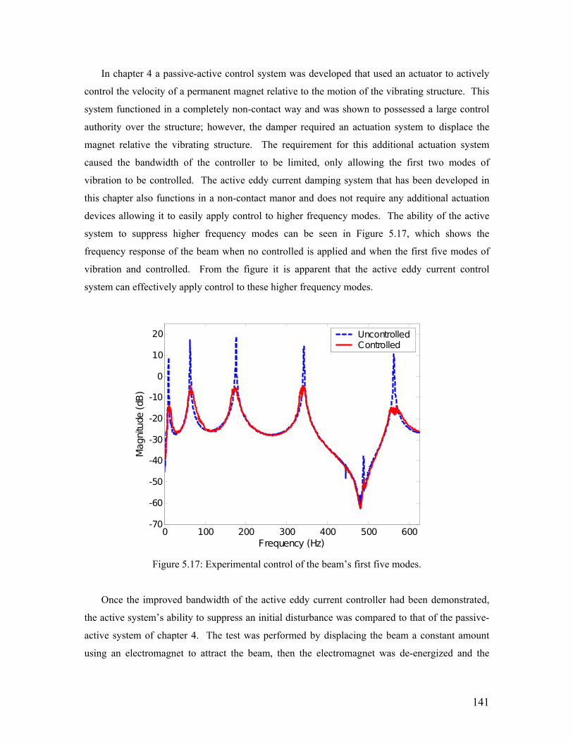
141

In chapter 4 a passive-active control system was developed that used an actuator to actively

control the velocity of a permanent magnet relative to the motion of the vibrating structure. This

system functioned in a completely non-contact way and was shown to possessed a large control

authority over the structure; however, the damper required an actuation system to displace the

magnet relative the vibrating structure. The requirement for this additional actuation system

caused the bandwidth of the controller to be limited, only allowing the first two modes of

vibration to be controlled. The active eddy current damping system that has been developed in

this chapter also functions in a non-contact manor and does not require any additional actuation

devices allowing it to easily apply control to higher frequency modes. The ability of the active

system to suppress higher frequency modes can be seen in Figure 5.17, which shows the

frequency response of the beam when no controlled is applied and when the first five modes of

vibration and controlled. From the figure it is apparent that the active eddy current control

system can effectively apply control to these higher frequency modes.

0 100 200 300 400 500 600-70

-60

-50

-40

-30

-20

-10

0

10

20

Frequency (Hz)

Mag

nitu

de (dB

)

UncontrolledControlled

Figure 5.17: Experimental control of the beam’s first five modes.

Once the improved bandwidth of the active eddy current controller had been demonstrated,

the active system’s ability to suppress an initial disturbance was compared to that of the passive-

active system of chapter 4. The test was performed by displacing the beam a constant amount

using an electromagnet to attract the beam, then the electromagnet was de-energized and the

142

beam was released from its initial displacement and allowed to vibrate freely. Once the beam

begins to vibrate, the controller works to quickly suppress the vibration. A typical experimentally

measured controlled response to an initial condition is shown in Figure 5.18 for both the passive-

active system, and the fully active system. From this figure it can be seen that the active control

system can effectively suppress the vibration of the beam, and that the settling time is comparable

to that of the passive-active damper. Therefore, in addition to having a larger bandwidth than the

passive-active controller, the active system is much smaller and can effectively suppress an initial

disturbance.

0 0.2 0.4 0.6 0.8 1 1.2-1

-0.5

0

0.5

1

1.5

Dis

pla

cem

ent (

mm

)

0 0.2 0.4 0.6 0.8 1 1.2-5

0

5

Time (sec)

Dis

plac

emen

t (m

m)

Active Control

Passive-Active Control

Figure 5.18: Initial displacement response of the beam with the active controller and the passive-

active damper developed in chapter 4.

5.5 Chapter Summary

Eddy currents are formed when a conductive material is subjected to a time varying magnetic

flux. This time changing flux can be formed in various different ways, for instance the eddy

currents used in chapter 2 and 3 were formed due to the motion of the conductor in a static

magnetic field. In chapter 5, the eddy currents are induced by actively varying the current applied

143

to an electromagnet. As the current changes, the magnetic flux is also modified allowing eddy

currents to form in the conductor. By utilizing a sensing system to monitor the vibration of the

beam, a compensator can be applied in the feedback loop to actively control the current applied to

the electromagnet and thus the forces induced on the beam, allowing the vibration to be

suppressed.

This chapter has begun by deriving the equations necessary to determine the eddy currents

induced in the conductive material. For the actuation system considered here, a time changing

magnetic flux is induced on the conductor by two sources. The first is due to the motion of the

conductor in the magnetic field generated by the electromagnet and the second is due to the time

varying current applied to the electromagnetic coil. Once the equations defining the eddy current

density had been derived, the force applied to the structure due to the interaction between the

eddy currents and the applied magnetic field could be found. The equations defining the eddy

current force result in an interesting finding; that the force applied to the beam is at twice the

frequency as the current applied to the electromagnet. This effect, while fascinating, leads to

difficult control issues that arise due to the need for the control force to be at relatively the same

frequency as the structures vibration. However, this means that the current applied to the beam

must be at half the frequency of the sensing signal, which requires an additional transfer function.

Once the issues associated with the frequency doubling affect were identified and corrected, the

control system was formulated. The compensators were designed to be second order filters with a

free derivative in the numerator to account for an integration performed in the algorithm to reduce

the sensing frequency by half.

Subsequent to the identification of an algorithm that easily allowed the frequency of the

sensor signal to be reduced by half, the compensator’s parameters could be tuned. The equations

governing the eddy currents induced in the beam are very nonlinear making them very difficult to

analytically model. Therefore, a numerical simulation of the complete system was performed to

predict the ideal filter parameters to be used in the experiments. Once the filters had been tuned

in the simulation, an experimental setup was constructed that consisted of a cantilever aluminum

beam with an electromagnet positioned a small distance from its surface. The active control

system was implemented using a real time data acquisition system that allowed the filter

parameters to be quickly modified. The parameters predicted in the theoretical model were

initially used in the experiments to obtain the correct location of the parameters and were then

tuned to provide the most vibration suppression.

144

After identifying both the predicted and experimentally tuned filter values, a comparison of

the values revealed a significant amount of variation between the two. Therefore, it was

determined that the numerical simulation of the system had neglected some important dynamics

in the experimental setup. In order to identify the neglected dynamics, the transfer function

between the input and output of each component was measured. These tests showed that the

equipment was all accounted for in the numerical simulation and left only the dynamics of the

electromagnetic coil to blame. The last experiment performed identified the transfer function

between the current applied to the coil and the magnetic field generated. Once this relation was

modeled and included in the simulation, it was found that the predicted filter parameters were

almost identical to the tuned values for in the experiments. This result showed that the dynamics

of the coil could be not neglected. Once the numerical simulation was shown to be accurate, the

performance of the active eddy current control system was identified. It was shown that the

active controller could suppress the cantilever beam’s first mode of vibration by more than 97%

and the second mode by approximately 96.6%. Furthermore, the active system was compared to

the passive-active controller developed in chapter 4. One of the major limitations of the passive-

active control system was that it required an additional actuation device to displace a permanent

magnet relative to the beam. The actuator that was chosen in chapter 4 limited the controller’s

bandwidth to only the first two modes of vibration. Therefore to show the increased bandwidth

of the active system, control was applied to the beam’s first five modes of vibration with an

average attenuation of approximately 25dB. Additionally, it was shown that the active system

could suppress an initial displacement with a comparable settling time.

145

Chapter 6

Conclusions

The optical power of satellites such as the Hubble telescope is directly related to the size of the

primary mirror. However, due to the limited capacity of the shuttle bay, progress towards the

development of more powerful satellites using traditional construction methods has come to a

standstill. Therefore, to allow larger satellites to be launched into space the Air Force, NASA and

DARPA have shown significant interest in the development of ultra large inflatable structures

that can be packaged inside the shuttle bay and then deployed once in space. To facilitate the

packaging of the inflated device in its launch configuration, most structures utilize a thin film

membrane as the optical or antenna surface. Once the inflated structure is deployed in space, it is

subject to vibrations induced mechanically by guidance systems and space debris as well as

thermally induced vibrations from variable amounts of direct sunlight. For the optimal

performance of the satellite, it is crucial that the vibration of the membrane be quickly

suppressed. However, due to the extremely flexible nature of the membrane structure, few

actuation methods exist that avoid local deformation and surface aberrations.

Realizing the severe limitations posed by the presently available actuation techniques, this

dissertation has sought to develop new actuation methods capable of fulfilling the requirements of

inflatable structures. The search for applicable actuation methods has lead to the development of

systems that utilize a variety of active materials such as PZT, terfenol-D, electro-rheological,

magneto-rheological, and shape memory alloys. However, one method of providing vibration

suppression that has not seen significant research is eddy current damping. Dampers of this type

function through the eddy currents that are generated in a conductive material experiencing a time

changing magnetic field. The density of these currents is directly related to the velocity of the

conductor in the magnetic field. However, following the generation of these currents, the internal

146

resistance of the conductor causes them to dissipate into heat. Because a portion of the moving

conductor’s kinetic energy is used to generate the eddy currents, which are then dissipated, a

damping effect occurs. This damping force can be described as a viscous force due its

dependence on the velocity of the conductor.

While eddy currents form an effective method of applying damping, they have normally been

used for magnetic braking applications. Furthermore, the dampers that have been designed for

vibration suppression have typically been ineffective at suppressing structural vibration (Zheng et

al. 2003), incompatible with practical systems, and cumbersome to the structure resulting in

significant mass loading and changes to the dynamic response (Kwak et al. 2004). To alleviate

these issues, this dissertation has identified three previously unrealized damping mechanisms that

function through eddy currents and has developed the necessary modeling techniques required to

design and predict the performance of each. The dampers do not contact the structure, thus,

allowing them to add damping to the system without inducing the mass loading and added

stiffness that are typically common with other forms of damping. The first damping concept is

completely passive and functions solely due to the conductor’s motion in a static magnetic field.

The second damping system is semi-active and improves the passive damper by allowing the

magnet’s position to be actively controlled, thus, maximizing the magnet’s velocity relative to the

beam and enhancing the damping force. The final system is completely active and uses an

electromagnet, through which the current can be actively modified to induce a time changing

magnetic flux on the beam and a controlled damping effect.

6.1 Brief Summary of Dissertation and Results

This dissertation has investigated the development of three new vibration control mechanisms

that function through the eddy currents generated in a conductive material that is subjected to a

time varying magnetic flux. This time varying magnetic flux can be induced on the material in

several different ways, each of which has been used to design a new damping mechanism that has

not been previously demonstrated. In total, three dampers have been designed, modeled and

tested, each showing that it can apply significant damping to a vibrating structure. The first

damper that has been developed is of completely passive nature and does not require any

additional energy to be added into the system. This damping system functions by placing a

permanent magnet a small distance from the vibrating structure. Due to the structure’s vibration

147

in the static magnetic field, it experiences a time changing magnetic flux that induces eddy

currents in the material. The theoretical model necessary to predict eddy currents induced in the

conductor and the damping force generated was developed in chapter 2. Once the damping force

was identified, the eddy current damper was coupled into the equations of motion of both a beam

and a thin membrane under an axial load. This theoretical model was then validated through an

experimental analysis which has been presented in chapter 3. The first structure tested was a

cantilever beam and the results showed that the model could accurately predict the damping

induced on the structure and could apply significant vibration attenuation. For the first bending

mode of vibration, the damping ratio was predicted within 10% over a large range of gaps

between the magnet and the beam. Additionally, it was shown that damper could increase the

damping in the first mode of vibration from 0.2% to approximately 35%, an increase of over 175

times.

After identifying the performance of the passive system using a single magnet, an improved

damping concept was developed in chapter 3. This improved concept consisted of placing a

second magnet on the opposite side of the vibrating structure such that the two magnets had

similar poles facing one another. When two magnets with similar poles are brought into close

proximity, a force is generated due to the compression of the magnetic field in the poling

direction. This compression of the magnetic field results in an increased magnetic flux in the

radial direction and because the eddy current rely on the radial magnetic flux, the damping effect

is enhanced. This new system was modeled using the superposition of the two magnetic fields

and an experimental analysis was performed. The results of the study showed that once again the

model could predict the damping ratio within 10% and that the damper could apply more than

critical damping to the beam.

The last study performed that utilized the purely passive magnetic damper, investigated the

application of damping to a very thin membrane. The membrane structure is difficult to apply

control to due to its extreme flexibility, which causes typically actuation methods to results in

only local deformations. This issue if further complicated by the use of membranes as metrology

surfaces in deployable space structures. In applications such as these, the membrane must uphold

strict surface tolerances to perform optimally. However, the choice of actuation method becomes

very limited due to the bonding of an actuator to the surface of the membrane resulting in surface

aberrations that can hinder its performance. Because eddy current dampers function in a non-

contact manor, they can be utilized while avoiding these issues, thus forming an ideal membrane

148

vibration control mechanism. However, the eddy current damper is highly dependent on the

thickness of the conductive structure, raising the issue of whether sufficient control forces can be

generated in the extremely thin membranes used for space applications. Therefore, the last study

performed in chapter 3 was to identify the eddy current dampers ability to suppress the vibration

of a thin membrane. To do so, an experimental test rig was constructed and the passive damper

was tested at both ambient and vacuum pressure. It was shown that the theoretical model of the

membrane coupled with the eddy current damper could effectively predict the induced damping,

and that the damper could generate approximately 30% damping at ambient pressure and upwards

of 25% damping at vacuum pressures. These results illustrate both the dampers compatibility

with thin membranes and their functionality in high atmospheric and space applications

Subsequent to the development of the passive eddy current damper, a novel damping concept

was developed that combined and active component into the passive system. In the passive

damper the conductor’s motion in a static magnetic field allowed the eddy current to form. The

new passive-active damper functions by providing the magnet with the ability to change its

position relative to the beam, such that the net velocity between the beam and magnet can be

maximized and the damping force enhanced. The density of the eddy currents formed using this

damping system can be modeled in much the same way as the passive system but a feedback

control system must be designed to actively modify the magnet’s position relative to the motion

of the beam. The compensator in the feedback loop was designed to be a second order filter. The

closed loop transfer function of the complete dynamic system was identified and shown to be

stable for a finite range of gains. Following the development of the theoretical closed loop

transfer function, an experiment was developed to validate the model and identify the

performance if the system. To actively displace the magnet, an electromagnetic shaker was used

because it was readily available; however this actuator could only effectively displace the magnet

up to 100Hz, thus limiting control to the first two modes. The results of these experiments

showed that the predicted tuned filter parameters matched those found in the laboratory and that

the measured closed loop frequency response was in excellent agreement with the theory.

Furthermore, it was demonstrated that the passive-active control system could effectively

suppress the vibration of the cantilever beam’s first bending mode by approximately 27dB and

the second bending mode by approximately 25dB.

The third and last eddy current damping mechanism is a completely active control system

that utilizes an electromagnet. In the two previously discussed eddy current dampers, a

149

permanent magnet was used and the eddy currents were induced due to a net velocity between the

structure and the static magnetic field. The active system subjects the conductive material to a

time changing magnetic flux by actively varying the current flowing through an electromagnet,

which allows the intensity of the magnetic field around the conductor to be controlled. The

equations defining the density of the eddy currents formed have been derived for this new damper

in chapter 5. However, because the conductor is also moving or vibration in the time varying

field generated by the electromagnet, both the motional eddy currents and the transformer eddy

currents must be accounted for. The resulting equations identified an interesting effect; that the

force induced on the beam due to the formation of the eddy currents is at twice the frequency of

the current applied to the electromagnet. This frequency doubling effect requires the feedback

control system to divide the sensor signals frequency by half, such that the control current is at

half the sensor frequency and the resulting control force is at the frequency of vibration. An

algorithm to perform this frequency reduction was designed along with a feedback compensator.

Due to the nonlinearities involved with the active control system the closed loop response could

not be analytically solved and required a numerical simulation to be performed.

Following the theoretical development of the system’s closed loop response, experiments

were performed to validate the derived model. The first experiment demonstrated that the

frequency doubling effect did occur, thus validating the correctness of the derived equations.

Next, the transfer function defining the relation between the current applied to the electromagnet

and the resulting magnetic field was experimentally measured and included into the numerical

simulation. With this relationship known, the numerical model was used to predict the tuned

values of the filter parameters, which were then compared to those identified through

experiments. The results showed that when the transfer function defining the coil dynamics was

included into the simulation, the predicted parameters were nearly identical to the measured ones.

The active control system was also shown to effectively suppress the beam’s first mode of

vibration by more than 97% and the second mode of vibration by approximately 96.6%.

Furthermore, the performance of the active eddy current control system was compared to that of

the passive-active system. The results of this comparison showed that the active system could

suppress an initial disturbance with a comparable settling time and that it could apply vibration

control to higher frequency modes (control was applied to the first five bending modes of the

beam with an average suppression of 25 dB), were as the passive-active system was limited by

the actuation system chosen.

150

6.2 Contributions

In most applications, the additional mass and stiffness that are induced due to the use of a

vibration damper, while undesirable are not major design criteria. However, in recent years there

has been a growing interest in the development of ultra large lightweight deployable structures.

Because these structures are deployable, they are packaged in their launch configuration and

deployed once in space. The packaging of the satellite leads to the requirement that the

metrology surface be flexible and has typically been a very thin membrane. Because this

membrane is to be used as a metrology surface it must hold extremely strict surface tolerances

which can easily be exceeded if the membrane is subjected to structural vibrations. This

requirement that the membrane must be free of vibration for it to perform optimally, leads to

difficult control issues brought on by the membranes extremely flexible nature. The extreme

flexibility places severe limitations on the actuation methods compatible with the membrane.

These limitations are due to the fact that the bonding of an actuator to the membrane can result in

surface aberrations and that if a point actuation method were used, only local deformations would

result. The eddy current effect can lead to an ideal damping mechanism, however due to the

ineffectiveness of the previously developed eddy current damping mechanisms; their potential

has not been realized. Therefore, my research has identified three previously unknown methods

of applying damping to a vibrating structure, and has developed the necessary modeling

techniques required to design and predict the performance of each.

This dissertation has developed three new methods of applying vibration suppression to a

structure, each of which has not been previously identified. Each of these dampers functions

through the eddy currents that are formed when a conductive material experiences a time varying

magnetic flux. This time changing magnetic flux can be generated in several different ways, each

of which will be used to identify a new damping mechanism. Because the damping mechanisms

function through magnetic fields, they can be made such that they apply damping forces without

ever coming into contact with the structure, a feature unique to the described eddy current

damper. This property allows the dampers to be applied without inducing mass loading or added

stiffness, which are typical downfalls of other means of damping. Furthermore, the non-contact

properties allow these dampers to be applied to the very thin membranes used in inflatable

satellite applications without causing surface imperfections or localized deformations, which are

unavoidable when using other damping systems, and result in non-optimal performance.

151

The first damper is of completely passive nature that after a thorough literature review was

determined to be the only existing passive non-contact damping system. Most typical eddy

current damping mechanisms have been developed such that the motion of the conductor is

perpendicular to the poling axis of the magnet. This particular configuration, while able to

generated significant damping forces, is not ideal for use in structural vibration applications due

the necessity to fix a cumbersome device to the structure. The passive damper developed in this

dissertation function such that the motion of the conductor is in the poling direction of the

magnet. This subtle difference allows the new damper to be both easily installed into the system

and to apply damping forces in a non-contact manor. Furthermore, this dissertation has derived

and validated the theoretical model necessary to predict the density of the eddy currents formed

and the damping induced on the vibrating structure by the passive system.

Furthermore, this dissertation has developed a second passive damper that can apply

significantly more vibration to the structure by placing a second magnet on the opposite side of

vibrating structure as the first, such that they have similar poles facing each other. This improved

damping concept was theoretically modeled and experimentally validating showing the

significant improvement in damping, and the validity of the model. In addition to developing a

new passive eddy current damper and the necessary theoretical model to predict the systems

interaction with a vibrating structure, the passive damper has been shown to be effective for the

suppression of membrane vibrations. Because the eddy currents induced in the structure are

dependent on the thickness of the conductive material it was questionable as to whether sufficient

damping forces could be generated to suppress the membranes vibration. Through both a

theoretical and experimental evaluation of the damping force induced, it was shown that the

vibration of the structure could be effectively suppressed. This provided the first demonstration

of the compatibility of eddy current damping mechanisms and extremely thin membranes.

Following the development of the new passive damping system, the concept was combined

with an active component to form a novel passive-active damper. The passive-active system

utilizes an actuator and compensator to actively modify the position of the magnet relative to the

vibrating structure. Using this system the net velocity between the magnet and the beam and the

rate of change in the magnetic flux applied to the conducting structure can be controlled such that

the damping force can be maximized. A magnetic damping system that functions by actively

controlling the velocity of a static magnetic field relative the structure has never before been

152

studied, making this system the first of its kind. The passive-active control system has been

analytically modeled using a linearization of the damping force. This model has also been

validated through experiments that showed the model’s linearization to be accurate and the

predicted closed loop dynamics to be extremely well represented by the model. This passive-

active control system also performs in a non-contact fashion making it ideal for use with

lightweight structures.

Lastly, a new completely active damping concept has been developed. This damper works by

controlling the current flowing through an electromagnetic coil such that a time varying magnetic

field is generated. A full theoretical model of this system was derived and revealed an interesting

result that could not be found in the existing literature. It was found that the force induced on the

conductive structure is at twice the frequency as the current applied to the coil. Because this

result had not been shown before, an experiment was performed and demonstrated that it

prediction was correct. Using this concept, a feedback compensator was designed such that it

could reduce the sensing frequency by half and apply control only to a narrow band of

frequencies around a resonant peak. This control system allowed the active eddy current damper

to effectively suppress the vibration of the structure. While a structure subjected to a time

changing magnetic field has been investigated previously (Tani et al. 1990, Morisue 1990, Tsuboi

et al. 1990, Takagi et al. 1992, and Takagi and Tani 1994), the modeling had been performed

using finite elements and was not used for vibration control. Therefore, the theoretical model,

and vibration damping mechanism are both contributions to the field.

This dissertation has made numerous contributions in the design, modeling and development

of new vibration suppression methods. Each of the three dampers developed represents a new

technology and the accompanying modeling techniques provides a method for future researchers

to design the mechanism before its construction. This is a major advance because due to the lack

of design tools currently available, eddy current dampers are built in an ad hoc way causing them

to be expensive to construct. Additionally, the three innovative damping mechanisms that have

resulted from this research apply control forces to the structure without contacting it, which

cannot be done by any other passive vibration control system. The non-contact nature of the

damper allows them to be easily applied while avoiding mass loading and added stiffness, which

is a common downfall of other damping methods. Furthermore, the dampers developed are also

ideal for use in space because they have a low dependence on temperature, are frictionless and

require no maintenance, and use only metallic materials alleviating issue with out gassing a seals

153

that may leak. For these reasons and the non-contact nature of the dampers, they are compatible

with the flexible membranes needed to advance the performance of optical satellites.

6.3 Recommendations for Future Work

This dissertation has developed three new eddy current damping mechanisms, each of which

functions differently. A theoretical model of each damper was derived and experiments were

performed to validate each model. The results of these tests showed that the models accurately

predicted the response of the system. However, because this research has mainly focused on the

design and development of these damping mechanisms, there are still some topics that could be

further researched. In the case of the passive system the model developed should be used to

optimize the design a magnetic damper. An optimization of the damping mechanism would

allow important design criteria to be identified, thus allowing design engineers to select only

important parameters.

In the case of the passive-active and the fully active systems, the damping force induced is

very nonlinear; however a linear compensator was used for the control system, which could

potentially provide less than optimal performance to the nonlinear system. Therefore, it is

necessary that a nonlinear controller be designed for each of these systems to determine if

additional damping could be achieved. In the case of the active system a more accurate

measurement of the relationship between the applied current and the generated magnetic field

should be made to improve the accuracy of the model.

Lastly, each of the damping mechanism should be designed into a two dimensional

membrane system such that the effectiveness of these dampers for the suppression vibration in the

membranes used in inflatable structures can be identified. This final experiment will demonstrate

the functionality of the dampers for space applications provide the ground necessary to pursue

their development further.

154

Bibliography

Agnes, G.S. and Rogers, J.W., 2000, “Piezoelectric Excitation of Inflatable Space Structures for

Modal Testing,” Proceedings of SPIE’s 7th Annual Smart Materials and Structures Conference,

Vol. 3985-88, Newport Beach, CA, pp. 806-819.

Allemang, R.J. and Brown, D.L., 1998, “A unified Matrix Polynomial Approach to Modal

Identification,” Journal of Sound and Vibration, Vol. 211, No. 3, pp. 301-322.

Bae, J.S., Kwak, M.K., and Inman, D. J., 2004, “Vibration Suppression of Cantilever Beam Using

Eddy Current Damper,” Journal of Sound and Vibration, submitted.

Bailey, T. and Hubbard Jr., J.E., 1985, “Distributed Piezoelectric-Polymer Active Vibration

Control of a Cantilever Beam,” Journal of Guidance and Control, Vol. 8, No. 5, pp. 605-611.

Bales, G.L., Hall, J.L., Flint, E.M. and Glease, R.M., 2003, “Experimental Issues that Impact In-

Vacuum Dynamic Characterization of Thin Film Membranes,” AIAA Paper No. 2003-1743,

Proceeding of the 44th AIAA/ASME/ASCE/AHS Structures, Structural Dynamics and Materials

Conference, April 7-10, Norfolk, VA.

Baz, A., Poh, S. and Studer, P., 1987, “Optimum Vibration Control of Flexible Beams by Piezo-

Electric Actuators,” Proceedings of the Sixth VPI & SU/AIAA Symposium on Dynamics and

Control of Large Structures, June 29th-July 1st, Blacksburg, VA, pp. 217-234.

Baz, A. and Poh, S., 2000, “Performance Characteristics of the Magnetic Constrained Layer

Damping,” Shock and Vibration, Vol. 7, pp. 81-90.

155

Blandino, J.R., Pappa, R.S., and Black J.T., 2003, “Modal Identification of Membrane Structures

with Videogrammetry and Laser Vibrometry, AIAA Paper No. 2003-1745, Proceeding of the 44th

AIAA/ASME/ASCE/AHS Structures, Structural Dynamics and Materials Conference, April 7-10,

Norfolk, VA.

Briand, G., Wicks, A.L. and Inman, D.J., 2000, “Vibration Testing for Control of Inflated

Objects,” Proceedings of the 18th International Modal Analysis Conference, San Antonio, Texas,

February.

Cadwell, L.H., 1996, “Magnetic Damping: Analysis of an eddy current brake using an air track,”

Journal of Physics, Vol. 64, pp. 917-923.

Cambell, J.D., 1956, “On the Theory of Initially Tensioned Circular Membranes Subjected to

Uniform Pressure,” Quarterly Journal of Mechanics and Applied Mathematics, Vol. 9, pp. 84-93.

Chein, W.Z., 1948, “Asymptotic behavior of a Thin Clamped Plate under Uniform Normal

Pressure at Very Large Deflection,” Experimental Stress Analysis Part 2, pp. 139-146.

Cheng, D. K., 1992, Field and Wave Electromagnetics, Addison-Wesley Publishing Company.

Chopra, I., 2002, “Review of State of Art Smart Structures and Integrated Systems,” AIAA

Journal, Vol. 40, No. 11, pp. 2145-2187.

Claflin, E.S. and Bareket, N., 1986, “Configuring an Electrostatic Membrane Mirror by Least-

Squares Fitting with Analytically Derived Influence Functions,” Journal of the Optical Society of

America, A. Optical and Image Science, Vol. 3, No. 11, pp. 1833-1839.

Crawley, E. and Anderson, E., 1990, “Detailed Models of Piezoceramic actuation of beams,”

Journal of Intelligent Material Systems and Structures, Vol. 1, No. 1, pp. 4-25.

Crawley, E.F. and de Luis, J., 1985, “Use of Piezo-Ceramics as Distributed Actuators in Large

Space Structure,” Proceeding of the 26th AIAA/ASME/ASCE/AHS Structures, Structural

Dynamics and Materials Conference, April 15-17th, Orlando, Florida, pp. 126-133.

156

Cugat, O., Mounaix, P., Basrour, S., Divoux, C. and Reyne, G., 2000, Deformable Magnetic

Mirror for Adaptive Optics: First Results,” Proceedings of the 13th Annual International

Conference on Micro-Electro-Mechanical Systems, Miyazaki, Japan, pp. 485-490.

Cunningham, R.E., 1986, Passive Eddy current Damping as a Means of Vibration Control in

Cryogenic Turbomachinery,” NASA Technical Paper number NASA-TP-2562, Access No. N86-

24722.

Davis, L.C. and Reitz, J.R., 1971, “Eddy Currents in Finite Conducting Sheets,” Journal of

Applied Physics, Vol. 42, No. 11, pp. 4119-4127.

De Blonk, B., 2003, “Selecting Models to Predict the Optical-Level Behavior of Membrane

Primary Mirrors,” AIAA Paper No. 2003-1653, Proceeding of the 44th AIAA/ASME/ASCE/AHS

Structures, Structural Dynamics and Materials Conference, April 7-10, Norfolk, VA, Vol. 3, pp.

2298-2308.

Dharamsi, U.K., Evanchik, D.M. and Blandino, J.R., 2002, Comparing Photogrammetry with a

Conventional Displacement Measurement Technique on a 0.5m Square Kapton Membrane,”

AIAA Paper No. 2002-1258, Proceeding of the 43th AIAA/ASME/ASCE/AHS Structures,

Structural Dynamics and Materials Conference, April 22-25, Denver, CO.

Dickey, R.W., 1967, “The Plane Circular Elastic Surface under Normal Pressure,” Archives for

Rational Mechanics and Analysis, Vol. 26, pp. 219-236.

Divoux, C., Cugat, O., Basrour, S., Mounaix, P., Kern, P. and Boussey-Saïd, J., 1998,

“Miniaturized Deformable Magnetic Mirror for Adaptive Optics,” Proceedings of the SPIE

Conference on Adaptive Optical System Technologies; Part 2, Kona, HI, USA, Vol. 3353, No. 2,

pp. 850-857.

Fanson, J.L. and Caughey,T.K., 1987, “Positive Position Feedback Control for Large Space

Structures,” AIAA Paper No. 87-0902, Proceeding of the 28th AIAA/ASME/ASCE/AHS

Structures, Structural Dynamics and Materials Conference, April 9-10th, Monterey, CA, pp. 588-

598.

157

Flint, E.M. and Glease, R.M., 2001, “Characterization, Prediction, and Improvement of Stretched

Flat Hexagonal Gossamer Membrane Dynamic Response,” AIAA Paper No. 2001-1410,

Proceeding of the 42nd AIAA/ASME/ASCE/AHS Structures, Structural Dynamics and Materials

Conference, April 16-19, Seattle, WA, USA.

Flint, E., Bales, G., Glease, R. and Bradford, R., 2003, “Experimentally Characterizing the

Dynamics of 0.5m+ Diameter Doubly Curved Shells Made from Thin Films, AIAA Paper No.

2003-1831, Proceeding of the 44th AIAA/ASME/ASCE/AHS Structures, Structural Dynamics

and Materials Conference, April 7-10, Norfolk, VA, USA.

Fredrick, J.R. and Darlow, M.S., 1994, “Operation of an electromagnetic Eddy Current Damper

wit a Supercritical Shaft,” ASME Journal of Vibration and Acoustics, Vol. 116, No. 4, pp. 578-

580.

Freeland, R.E., Bilyeu, G.D. Veal, G.R., Steiner, M.D. and Carson, D.E., 1997, “Large Inflatable

Deployable Antenna Flight Experiment Results,” Acta Astronautica, Vol. 41, No. 4-10. pp. 267-

277.

Freeland, R.E., Bilyeu, G.D. Veal, G.R. and Mikulas, M.M., 1998, “Inflatable Deployable Space

Structures Technology Summary,” International Astrological Association.

Fung, R-F., Sun, J-H. and Hsu, S-M., 2002, “vibration control of the Rotating Flexable-

Shaft/Multi-Flexable-Disk System with the Eddy-Current Damper,” ASME Journal Of Vibrations

and Acoustics, Vol. 124, pp. 519-526.

Graves, K.E., Toncich, D. and Ionvenitti, P.G., 2000, “Theoretical Comparison of the Motional

and Transformer EMF Device Damping Efficiency,” Journal of Sound and Vibration, Vol. 233,

No. 3, pp. 441-453.

Greschik, G., Mikulas, M.M. and Palisoc, A., 1998, Approximations and Errors in Pressurized

Axisymmetric Membrane Shape Predictions,” AIAA Paper No. 1998-2101, Proceeding of the

39th AIAA/ASME/ASCE/AHS Structures, Structural Dynamics and Materials Conference, Long

Beach, CA, USA, Vol. 4, pp. 2761-2771

158

Griffith, D.T. and Main, J.A., 2000, “Modal Testing of an Inflated Thin Film Polymide Torus

Structure,” Proceedings of the 18th International Modal Analysis Conference, San Antonio,

Texas, Febuary.

Grosso, Ronald P. and Yellin, Martin, 1977, “The membrane Mirror as an Adaptive Optical

Element,” Journal of the Optical Society of America, Vol. 67, No. 3, pp. 399-406.

Gunter, E.J., Humphris, R.R. and Severson, S.J., 1983, “Design Study of Magnetic Eddy-Current

Vibration Dampers for Application to Cryogenic Turbomachinery,” University of Virginia Report

UVA/528210/MAE84/101, NASA Grant NAG-3-263.

Hagood, N.W., Chung, W.H. and Von Flotow, A. 1990, “Modeling of Piezoelectric Actuator

Dynamics for Active Structural Control,” Journal of Intelligent Materials Systems and Structures,

Vol. 1, pp. 327-354.

Hahn, K.D., Johnson, E.M., Brokken, A. and Baldwin, S., 1998, “Eddy Current Damping of a

Magnet Moving Through a Pipe,” American Journal of Physics, Vol. 66, No. 12, pp. 1066-1076.

Hall J., Glease, R.M. and Flint, E., 2002, “Dynamic Behavior of Thin Film Membranes,” AIAA

Paper No. 2002-1378, Proceeding of the 43rd AIAA/ASME/ASCE/AHS Structures, Structural

Dynamics and Materials Conference, April 22-25th, Denver, CO.

Hanagud, S., Obal, M.W. and Meyyappa, M., 1985, “Electronic Damping Techniques and Active

Vibration Control,” AIAA Paper No. 85-0752, Proceeding of the 26th AIAA/ASME/ASCE/AHS

Structures, Structural Dynamics and Materials Conference, April 15-17th, Orlando, FL, pp. 126-

133.

Heald, M.A., 1988, “Magnetic Braking Improved theory,” American Journal of Physics, Vol. 56,

No. 6, pp.521-522.

Huang, S.C., Inman, D.J. and Austin, E.M., 1996, “Some Design Considerations for Active and

Passive Constrained Layer Damping Treatments,” Smart Structures and Materials, Vol. 5, pp.

301-313.

159

Juang J.N. and Hunag, W., 1983, “Static Shape Forming for an Electrostatically Controlled

Membrane Miror,” Proceedings of the American Control Conference, Vol. 3, pp. 1310-1316.

Jagourel, R., Madec, P. and Sechaud, M., 1990, “Adaptive Optics: A Bimorph Mirror for

Wavefront Correction,” Proceeding of the SPIE conference on Amplitude and Intensity Spatial

Interferometry, Tucson, AR, USA, Vol. 1237, pp. 394-405.

Jenkins, C.H., Wilkes, J.M. and Marker, D.K., 1998, “Improved Surface Accuracy of Precision

Membrane Reflectors Through Adaptive Rim Control,” AIAA Paper No. 1998-1983, Proceeding

of the 39th AIAA/ASME/ASCE/AHS/ASC Structures, Structural Dynamics, and Materials

Conference, Long Beach, CA, Vol. 3 pp. 2302-2308

Jenkins, C.H., 2001, “Gossamer Spacecraft: Membrane and Inflatable Structures Technology for

Space Applications,” American Institute of Aeronautics and Astronautics (AIAA), Reston, VA.

Kao, R., and Perrone, N., 1971, “Large Deflections of Axisymmetric Circular Membranes,”

International Journal of Solids and Structures, Vol. 7, pp. 1601-1612.

Kao, R., and Perrone, N., 1972, “Large Deflections of Flat Arbitrary Membranes,” Computers

and Structures, Vol. 2, pp. 535-546.

Karnopp, M., 1989, “Permanent Magnet Linear Motors Used as Variable Mechanical Damper for

Vehicle Suspensions,” Vehicle System Dynamics, Vol. 18, pp. 187-200.

Kienholtz, D.A., Pendleton, S.C., Richards, K.E. and Morgenthaler, D.R., 1994, “Demonstration

of Solar Array Vibration Suppression,” Proceedings of SPIE’s Conference on Smart Structures

and Materials, Orlando, FL, Feb. 14-16, Vol. 2193, pp. 59-72.

Kienholtz, D.A., Smith, C.A. and Haile, W.B., 1996, “A Magnetically Damped Vibration

Isolation System for a Space Shuttle Payload,” Proceeding of SPIE’s International Symposium on

Smart Structures and Materials, San Diego, CA, Vol. 2720, pp. 272-280.

160

Klingerman, Y., Gottlieb, O. and Darlow, M.S., 1998a, “Analytic and Experimental Evaluation of

Instability in Ratordynamic System wit Electromagnetic Eddy-Current Damper,” ASME Journal

of Vibrations and Acoustics, Vol. 120, pp. 272-278.

Klingerman, Y., Gottlieb, O. and Darlow, M.S., 1998b, “Nonlinear Vibration of a Rotating

System with an Electromagnetic Damper and a Cubic Restoring Force,” Journal of Sound and

Vibration, Vol. 4, pp. 131-144.

Kligerman, Y. and Gottlieb, O., 1998, “Dynamics of a Rotating System with a Nonlinear Eddy-

Current Damper,” Transactions of the ASME Journal of Vibration and Acoustics, Vol. 120, pp.

848-853.

Kobayashi, H. and Aida, S., 1993, Development of a Houde Damper using Magnetic Damping,”

Proceedings of the 14th Biennial ASME Conference on Vibration and Noise, Albuquerque, NM,

USA, Vol. 62, pp. 25-29.

Kwak, M.K., Lee, M.I. and Heo, S., 2003, “Vibration Suppression Using Eddy Current Damper,”

Korean Society for Noise and Vibration Engineering, in press.

Larose, G.L., Larsen, A. and Svensson, E., 1995, “Modeling of Tuned Mass Dapers for Wind

Tunnel Tests on a full-bridge areoelastic model,” Journal of Wind Engineering and Industrial

Aerodynamics, Vol. 54/55, pp. 427-437.

Lee, C.K., Chiang, W.W. and O’Sullivan, T.C., 1989, “Piezoelectric Modal Sensors and

Actuators Achieving Critical Active Damping on a Cantilever Plate,” AIAA Paper No. 89-1390-

CP, Proceeding of the 30th AIAA/ASME/ASCE/AHS Structures, Structural Dynamics and

Materials Conference, Mobile, Alabama, April 3-5th, pp. 2018-2026.

Lee, J.S., 1996, “Dynamic Stability of Beam Plates in Transverse Magnetic Fields,” Journal of

Engineering Mechanics, Vol. 122, No. 2, pp. 89-94.

Lee, K. and Park, K., 1999, “Optimal Robust Control of a Contact-less Brake System using an

Eddy Current, Mechatronics, Vol. 9 No. 6, pp. 615-631.

161

Lee, K. and Park, K., 2001a, “Modeling of the Eddy Currents with the Consideration of the

induced Magnetic Flux,” Proceeding of the IEEE International Conference on Electric and

Electronic Technology, Vol. 2, pp. 762-768.

Lee, K. and Park, K., 2001b, “Eddy Currents Modeling with the Consideration of the Magnetic

Reynolds Number,” Proceeding of the International Symposium on Industrial Electronics, Pusan,

South Korea, June 12-16, Vol. 1, pp. 678-683.

Lee, K. and Park, K., 2002, “Modeling Eddy Currents with Boundary Conditions by Using

Coulomb’s Law and the method of Images,” IEEE Transactions on Magnetics, Vol. 38, No. 2,

pp. 1333-1340.

Leigh, L., Hamidzadeh, H., Tinker, M. and Slade, K.N., 2001, “Dynamic Characterization of an

Inflatable Concentrator for Solar Thermal Propulsion,” AIAA Paper No. 2001-1406, Proceeding

of the 42nd AIAA/ASME/ASCE/AHS/ASC Structure, Structural Dynamics, and Material

Conference and Exhibit, Seattle, WA, April 16-19.

Main, J.A., Martin, J. and Nelson, G., 1999, “Noncontact Shape Control of Membrane Mirrors,”

Proceedings of the Ultra Lightweight Space Optics Challenge Workshop, Napa, CA, March 24–

25.

Marker, D.K. and Jenkins, C.H., 1997, “Surface Precision of Optical Membranes with

Curvature,” Optics Express, Vol. 1, No. 11, pp. 324-331.

Marker, D.K., Carreras, J.M., Wilkes, J.M., Jenkins, C.H., Duneman, D., Rotge, J.R. and Hogge,

C.B., 1998, “Optical Evaluation of Membrane Mirrors with Curvature,” Proceeding of the SPIE

Conference on Adaptive Concepts and Innovative Supporting Technologies for Large-Aperture

Imaging System, San Diego, CA, Vol. 3430, pp. 202-208.

Matsuzaki, Y., Ishikubo, Y., Kamita, T., and Ikeda, 1997, “Vibration Control System Using

Electromagnetic Forces,” Journal of Intelligent Material Systems and Structures, Vol. 8, pp. 751-

756.

162

Matsuzaki, T., Ikeda, T., Nae, A. and Sasaki, T., 2000, “Electromagnetic Forces for a New

Vibration Control System: Experimental Verification,” Smart Materials and Structures, Vol. 9,

No. 2, pp. 127-131.

Merkle, F., Freischalad, K. and Bille, J., 1981, “Development of an Active Optical Mirror for

Astronomical Application,” Presented at the ESO Conference on Scientific Importance of High

Angular Resolution at Infrared and Optical Wavelengths, Garching, Germany, March.

Morisue, T., 1990, “Analysis of a Coupled Problem: The Felix Cantilevered Beam,” IEEE

Transactions on Magnetics, Vol. 26, No. 2, pp. 540-543.

Nagaya, K., Kojima, H., Karube, Y. and Kibayashi, 1984, “Braking Force and Damping

Coefficient of Eddy Current Brakes Consisting of Cylindrical Magnets and Plate Conductors of

Arbitrary Shape,” IEEE Transactions on Magnetics, Vol. MAG-20, No. 6, pp. 2136-2145.

Oh, L., Ruzzene, M. and Baz, A., 1999, “Control of the Dynamic Characteristics of Passive

Magnetic Composites,” Composites Part B: Engineering, Vol. 30, pp. 739-751.

Oh, L., Poh, S., Ruzzene, M. and Baz, 2000, “Vibration Control of Beams Using Electro-

Magnetic Compressional Damping Treatment,” ASME Journal Vibration and Acoustics, Vol.

122, pp. 235-243.

Omer, A. and Baz, A., 2000, “Vibration Control of Plates Using Electromagnetic Compressional

Damping Treatment, Journal of Intelligent Material Systems and Structures, Vol. 11, pp. 791-

797.

Pappa, R.S., Giersch, L.R. and Quagliaroli, J.M., 2001, “Photogrammetry of a 5m Inflatable

Space Antenna with Consumer Digital Cameras,” Experimental Techniques, July/Aug. pp. 21-29.

Pappa, R.S., Jones, T.W., Black, J.T., Walford, A., Robson, S. and Shortis, M.R., 2002,

“Photogrammetry Methodology Development for Gossamer Spacecraft Structures,” Sound and

Vibration, Vol. 36, No. 8, 2002, pp. 12-21.

163

Pappa, R.S., Black, J.T., Blandio, J.R., Jones, T.W., Danehy, P.M. and Dorrington, A.A., 2003,

Dot-Projection Photogrammetry and Videogrammetry of Gossamer Space Structures,” Journal of

Spacecraft and Rockets, Vol. 40, No. 6, pp. 858-867.

Park, G., Kim, M.H. and Inman, D.J., 2001, “Integration of Smart Materials into Dynamics and

Control of Inflatable Space Structures,” Journal of Intelligent Materials Systems and Structures,

Vol. 12, No. 6, pp. 423-433.

Park, G., Ruggiero, E. and Inman, D.J., 2002, “Dynamic Testing of Inflatable Structures Using

Smart Materials,” Journal of Smart Materials and Structures, Vol. 11, pp. 1-9.

Perkins, W.P. and Rohniger, G., June 6, 1978, “Controlled Flexible Membrane Reflector,” U.S.

Patent Number 4,093,351.

Preliminary Mission Report, “Spartan 207/Inflatable Antenna Experiment Flown on STS-77,”

Spartan Project, Code 740.1, NASA Gaddard Space Flight Center, Greenbelt, MD, Febuary 14,

1997.

Rogers, J.W. and Agnes, G.S., 2002, “Modeling a Piezothermoeleastic Beam String,” Journal of

Spacecraft and Rockets, Vol. 39, No. 5, pp. 725-731.

Rogers, J.W. and Agnes, G.S., 2002, “Modeling a Piezothermoelastic Laminated Plate-

Membrane,” Journal of Intelligent Material Systems and Structures, Vol. 13, No. 5, pp. 303-316.

Rodgers, J.W. and Agnes, G.S., 2002, “Formulation of Asymptotic Finite Elements sing the

Method of Integral Multiple Scales,” AIAA Paper No. 2002-1663, Proceeding of the 43rd

AIAA/ASME/ASCE/AHS/ASC Structures, Structural Dynamics, and Materials Conference,

AIAA Gossamer Spacecraft Forum, April 22-25, Denver, CO.

Rogers, J.W. and Agnes, G.S., 2003, “Modeling Discontinuous Axisymmetric Active Optical

Membranes,” Journal of Spacecraft and Rockets, Vol. 40, No. 4, pp. 553-564.

Ruggiero, E., Park, G., Inman, D.J. and Main, J.A., 2002, “Smart Materials in Inflatable Structure

Applications,” AIAA Paper No. 2002-1563, Proceeding of the 43rd

164

AIAA/ASME/ASCE/AHS/ASC Structures, Structural Dynamics, and Materials Conference,

AIAA Gossamer Spacecraft Forum, April 22-25, Denver, CO.

Ruzzene, M., Oh, J. and Baz, A., 2000, “ Finite Element Modeling of Magnetic Constrained

Layer Damping, Journal of Sound and Vibration, Vol. 236, No. 4, pp. 657-682.

Schieber, D., 1974, “Braking Torque on Rotating Sheet in Stationary Magnetic Field,”

Proceedings of the Institution of Electrical Engineers, Vol. 121, No. 2, pp. 117-122.

Schieber, D., 1975, “Optimal Dimensions of Rectangular Electromagnet for Braking Purposes,”

IEEE Transactions on Magnetics, Vol. 11, No. 3, pp. 948-952.

Schmid, M. and Varga, P., 1992, “Analysis of Vibration-Isolating Systems for Scanning

Tunneling Microscopes,” Ultramicroscopy, Vol. 42-44, Part B, pp. 1610-1615.

Schmidt, R., 1974, “On Berger’s Method in the Non-Linear Theory of Plates,” Journal of Applied

Mechanics, Vol. 41, pp. 521-523.

Schmidt, R., and DaDeppo, D.A., 1974, “A New Approach to the Analysis of Shells, Plates and

Membranes with Finite Deflections,” International Journal of Non-Linear Mechanics, Vol. 9, pp.

409-419.

Shaker, F.J., 1975, “Effect of Axial Load on Modes and Frequencies of Beams,” NASA

Technical Note D-8109.

Shaw, F.S., Perrone, N., 1954, “A Numerical Solution for the Non-Linear Deflection of

Membranes,” Journal of Applied Mechanics, Vol. 21, pp. 117-128.

Simeu, E. and Georges, D., 1996, “Modeling and Control of an Eddy Current Brake,” Control

Engineering Practice, Vol. 4, No. 1, pp. 19-26.

Slade, K.N., Tinker, M.L., Lassiter, J.O. and Engberg, R., 2001, “Dynamics of an Inflatable

Structure in Vacuum and Ambient Conditions,” AIAA Journal, Vol. 39, No. 5, pp. 894-901.

165

Sodano, H.A., Park, G. and Inman, D.J., 2004, Multiple Sensors and Actuators for Vibration

Suppression of an Inflated Torus, AIAA Journal of Rockets and Spacecraft, Vol. 42, No. 2.

Solter, M.J., Horta, L.G. and Panetta, A.D., 2003, “A Study of a prototype Actuator Concepts for

Membrane Boundary Control,” AIAA Paper No. 2003-1736, Proceeding of the 43rd

AIAA/ASME/ASCE/AHS/ASC Structures, Structural Dynamics, and Materials Conference,

AIAA Gossamer Spacecraft Forum, April 7-10, Norfolk, VA.

Sommerfeld, A., 1889, Proceedings of the London Mathematical Society, Vol. 28, pp. 395.

Takagi, T., Tani, J., Matsuda, S., and Kawamura, S., 1992, “Analysis and Experiment of

Dynamic Deflection of a Thin Plate with a Coupling Effect,” IEEE Transactions on Magnetics,

Vol. 28, No. 2, pp. 1259-1262.

Takagi, T. and Tani, J., Dynamic Behavior of a Plate in Magnetic Field by Full Coupling and

MMD Methods, IEEE Transactions on Magnetics, Vol. 30, No. 5, pp. 3296-3299.

Talami, H. and Iye, M., 1994, “Membrane Deformable Mirror for SUBARU Adaptive Optics,”

Proceedings of the SPIE Conference on Adaptive Optics in Astronomy, Vol. 2201, pp. 762-767.

Tani, J., Minagawa, M., Ohtomo, K. and Saigo, M., 1990, “Dynamic Behavior of Thin Plates

under Impulsive Magnetic Field,” IEEE Transactions on Magnetics, Vol. 26, No. 2, pp. 544-547.

Teshima H., Tanaka, M., Miyamoto,K., Nohguchi, K. and Hinata, K., 1997, “Effect of Eddy

Current Dampers on the Vibrational Properties in Superconducting Levitation Using Melt-

Processed YBaCuO Bulk Superconductors,” Physica C, Vol. 274, pp. 17-23.

Thomas, M. and Veal, G., 1984, “Highly Accurate Inflatable Reflectors,” AFRPL TR-84-021.

Tinker, M.L., 1998, “Passively Adaptive Inflatable Structure for the Shooting Star Experiment,”

AIAA paper No. 98-1986, pp. 2320-2326.

166

Tsubi, H., Tanaka, M. and Misaki, T., 1990, “Eddy current and Deflection Analysis of a thin

Plate in Time-Changing Magnetic Fields,” IEEE Transactions on Magnetics, Vol. 26, No. 5, pp.

1647-1649.

Wagner, J., 2000, “Optical Metrology of Adaptive Membrane Mirrors,” M.S. Thesis, U.S. Air

Force Institute of Technology, Wright-Patterson AFB, OH.

Weil, N.A. and Newmark, N.M., 1955, “Large Plastic Deformations of Circular Membranes,” Journal of Applied Mechanics, Vol. 22, pp533-538.

Wiederick, H.D., Gauthier, N., Campbell, D.A. and Rochon, P., 1987, “Magnetic Braking:

Simple theory and experiment,” American Journal of Physics, Vol. 55, No. 6, pp. 500-503.

Wouterse, J.H., 1991, “Critical Torque and Speed of Eddy Current Brake with Widley Seperated

soft Iron Poles,” IEE Proceedings. Part B, Electric Power Applications, Vol. 138, No. 4, pp. 153-

158.

Zheng, X.J., Zhou, Y.-H. and Miya, K., 2001, “An Analysis of Variable Magnetic Damping of a

Cantilever Beam-Plate with end coils in Transverse Magnetic Fields,” Fusion Engineering and

Design, Vol. 55, pp. 457-465.

Zheng, H., Li, M. and He, Z., 2003, “Active and Passive Magnetic Constrained Damping

Treatment,” International Journal of Solids and Structures, Vol. 40, pp. 6767-6779.

167

Appendix A

Elliptic Integrals Associated with the Magnetic Flux of a

Cylindrical Permanent Magnet

168

The integrals defining the magnetic flux density of the cylindrical permanent magnet are

derived in chapter 2 and contain the elliptical integrals provided below. These integrals are too

difficult to solve analytically and must therefore be computed using numerical integration

techniques. The magnetic flux density in the y-direction defined in equation 2.10 contains the

integration I1 defined by

( )

⎥⎦

⎤⎢⎣

⎡

⎭⎬⎫

⎩⎨⎧

⎟⎠⎞

⎜⎝⎛ −

+⎟⎠⎞

⎜⎝⎛ −

−⎭⎬⎫

⎩⎨⎧

⎟⎠⎞

⎜⎝⎛ −

+⎟⎠⎞

⎜⎝⎛ −

=

−+= ∫

22222

21212

2

2

0 2322

1

4,4

34,4

4,4

34,4

1

sin2

sin

nybE

nybEp

nybE

nybEm

bynp

dybzb

I

ππππ

φφ

φπ

(A1)

where terms m2, n2 and p2 are defined as

2222 zybm ++= (A2)

( ) 222 zybn +−= (A3)

( ) 22 zybp ++= (A4)

where b is the radius of the permanent magnet and y and z are the position in the radial and poling

directions, respectively. The elliptic integrals of equation A1 are written as

( ) ( )∫ −==φ

θθφ0

2121 sin1, dmmE (A5)

( ) ( )∫−

−==φ

θθφ0

2122 sin1, dmmE (A6)

The magnetic flux density in the z-direction defined in equation 2.11 contains the integration I2

defined as

( )

⎥⎦

⎤⎢⎣

⎡

⎭⎬⎫

⎩⎨⎧

⎟⎠⎞

⎜⎝⎛ −

+⎟⎠⎞

⎜⎝⎛ −

+⎭⎬⎫

⎩⎨⎧

⎟⎠⎞

⎜⎝⎛ −

+⎟⎠⎞

⎜⎝⎛ −

=

−+

−= ∫

22222

21212

2

0 2322

2

4,4

34,4

4,4

34,4

1

sin2

sin

nybE

nybEp

nybE

nybEs

bnp

dybzb

ybI

ππππ

φφ

φπ

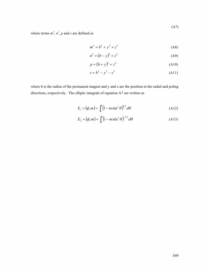
169

(A7)

where terms m2, n2, p and s are defined as

2222 zybm ++= (A8)

( ) 222 zybn +−= (A9)

( ) 22 zybp ++= (A10)

222 zybs −−= (A11)

where b is the radius of the permanent magnet and y and z are the position in the radial and poling

directions, respectively. The elliptic integrals of equation A7 are written as

( ) ( )∫ −==φ

θθφ0

2121 sin1, dmmE (A12)

( ) ( )∫−

−==φ

θθφ0

2122 sin1, dmmE (A13)

170

Vita

Henry A. Sodano was born on October, 4 1979 to parents Henry and Peggy Sodano in

Fairfax, Virginia. He graduated from Robinson Secondary School in June 1998 and began his

first year of collage with a major of Mechanical Engineering at Virginia Tech in August of that

year. Following four years of undergraduate study, he received his Bachelors of Science in

Mechanical Engineering in May of 2002. After the completion of his undergraduate program he

was invited to perform summer research at the Center for Intelligent Material Systems and

Structures (CIMSS) at Virginia Tech. The work that he performed during that summer, earned

him a graduate research position, and he began work on his master’s degree in the fall of 2002

under the direction of Dr. Daniel J. Inman. His research focus was in vibration control of

inflatable space structures and power harvesting using piezoelectric materials. In April of 2003

during the pursuit of his mater’s degree, Henry was awarded a NASA Graduate Student Research

Program fellowship (GSRP) to fund his efforts towards a Doctorate of Philosophy in Mechanical

Engineering beginning in August of 2003. He completed his Master of Science in Mechanical

Engineering on July 31st 2003, and began to work towards a Ph.D at Virginia Tech. The topic of

his Ph.D research has been in the development of vibration suppression mechanisms compatible

with the extremely thin membranes used with deployable satellites. After performing research in

the topic for approximately 21 months his research had lead to the development of three new

actuation methods, each of which applied control forces without contacting the structure.

Following the completion of his Ph.D, Henry looks forward to obtaining a faculty position in the

Mechanical Engineering Department at Michigan Technological University.

Postal Address:

310 Durham Hall

Virginia Tech mail code 261

Blacksburg, VA 24061