University of Tennessee, Knoxville University of Tennessee, Knoxville

TRACE: Tennessee Research and Creative TRACE: Tennessee Research and Creative

Exchange Exchange

Chancellor’s Honors Program Projects Supervised Undergraduate Student Research and Creative Work

5-2015

Development of an Efficient Data Processing Procedure for the Development of an Efficient Data Processing Procedure for the

Prediction of Cleavage Fracture in Reactor Pressure Vessel Steels Prediction of Cleavage Fracture in Reactor Pressure Vessel Steels

Using the J-AUsing the J-A22 Method Method

Phoebe E. Fogelman University of Tennessee - Knoxville, pfogelma@vols.utk.edu

Follow this and additional works at: https://trace.tennessee.edu/utk_chanhonoproj

Part of the Mechanics of Materials Commons

Recommended Citation Recommended Citation Fogelman, Phoebe E., "Development of an Efficient Data Processing Procedure for the Prediction of Cleavage Fracture in Reactor Pressure Vessel Steels Using the J-A2 Method" (2015). Chancellor’s Honors

Program Projects. https://trace.tennessee.edu/utk_chanhonoproj/1891

This Dissertation/Thesis is brought to you for free and open access by the Supervised Undergraduate Student Research and Creative Work at TRACE: Tennessee Research and Creative Exchange. It has been accepted for inclusion in Chancellor’s Honors Program Projects by an authorized administrator of TRACE: Tennessee Research and Creative Exchange. For more information, please contact trace@utk.edu.

Development of an Efficient Data Processing Procedure for the Prediction of Cleavage Fracture in

Reactor Pressure Vessel Steels Using the J-A2 Method

Phoebe E. Fogelman

College of Engineering

Department of Mechanical Engineering

Thesis Advisor: Dr. Larry Sharpe

Contents Abstract .......................................................................................................................................................... i

Table of Symbols and Abbreviations ............................................................................................................ ii

Table of Figures ........................................................................................................................................... iii

Introduction ................................................................................................................................................... 1

Background ............................................................................................................................................... 1

Mathematical Models ................................................................................................................................ 2

Purpose ...................................................................................................................................................... 3

Method .......................................................................................................................................................... 4

Description of Abaqus Model ................................................................................................................... 4

Data Processing ......................................................................................................................................... 6

Analysis of Deep-Cracked Specimen ....................................................................................................... 7

Results and Discussion ................................................................................................................................. 8

Process Validation .................................................................................................................................... 8

Deep-Cracked Specimen ......................................................................................................................... 10

Limitations and Future Directions .............................................................................................................. 11

Acknowledgements ..................................................................................................................................... 11

References ................................................................................................................................................... 12

i

Abstract

Nuclear power plants have played an important role in decreasing the world’s dependence on

fossil fuels.As structures age, however, the hazards of continued operation must be evaluated against the

cost of closure or refurbishment. The mechanism of failure for reactor pressure vessel steel is therefore of

great concern. Because the competing ductile and brittle failure mechanisms result in a stochastic process,

determination of critical values is computationally intensive. Finite element analysis is used to discretize

the problem and simulate loading conditions to characterize material behavior. The J-A2 method is a

proposed improvement on the Hutchinson, Rice, and Rosengren solution to the failure prediction

problem, which has a conservative bias. Because the J-A2 method relies on the solution of a quadratic

equation, however, the calculations are much more complicated. In order to continue validating this

method, numerous experimental data sets will have to be compared to simulated results. With the former

data structure and organization, this validation would be extraordinarily time-consuming, and delegating

to research assistants would require extensive training and troubleshooting. The purpose of this project

was therefore to develop a more automated and efficient method of processing data and demonstrate that

resulting calculations are equivalent to those obtained by the original procedure. Furthermore, an

additional data set is analyzed with the J-A2 method, and computed critical values are compared with

those experimentally determined at failure. The streamlined data processing procedure does, in fact,

generate the same prediction as the previous method when applied to shallow-cracked specimens in 3-

point bending. When used to analyze deep-cracked specimens, a curve fit is required to determine

properties at the intersection with the material failure curve.

ii

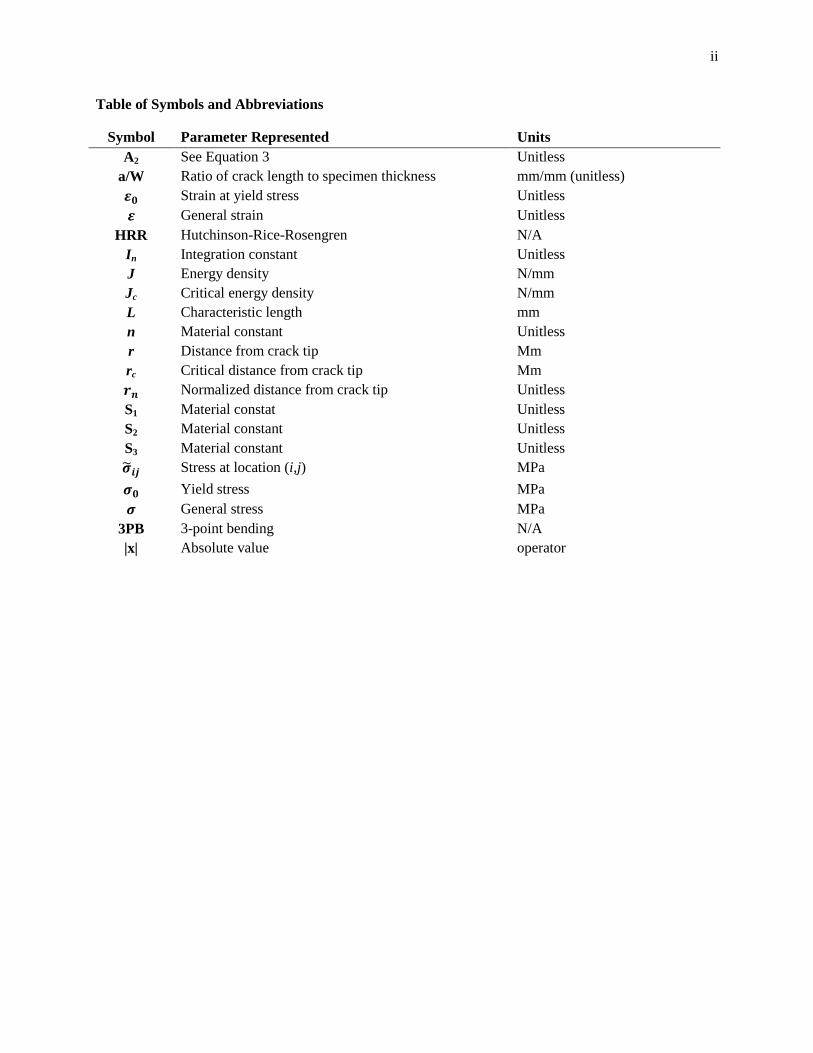
Table of Symbols and Abbreviations

Symbol Parameter Represented Units

A2 See Equation 3 Unitless

a/W Ratio of crack length to specimen thickness mm/mm (unitless)

Strain at yield stress Unitless

General strain Unitless

HRR Hutchinson-Rice-Rosengren N/A

In Integration constant Unitless

J Energy density N/mm

Jc Critical energy density N/mm

L Characteristic length mm

n Material constant Unitless

r Distance from crack tip Mm

rc Critical distance from crack tip Mm

Normalized distance from crack tip Unitless

S1 Material constat Unitless

S2 Material constant Unitless

S3 Material constant Unitless

Stress at location (i,j) MPa

Yield stress MPa

General stress MPa

3PB 3-point bending N/A

|x| Absolute value operator

iii

Table of Figures

Figure 1. Comparison of stress-strain curves for ductile and brittle materials………………….. 1

Figure 2. 3D rendering of shallow-cracked specimen…………………………………………… 4

Figure 3. Abaqus model of 3-Point Bending specimen with a shallow crack…………………… 4

Figure 4. (a) Specimen with mesh……………………………………………………………….. 5

Figure 4. (b) Detail view of mesh surrounding crack tip………………………………………... 5

Figure 5. Crack propagation path selected in Abaqus…………………………………………… 6

Figure 6. Abaqus model of 3-Point Bending specimen with a deep crack………………………. 7

Figure 7. Graphical representation of Excel analysis results for shallow-cracked specimen…… 9

Figure 8. Graphical representation of Matlab analysis results for shallow-cracked specimen….. 9

Figure 9. Graphical representation of results from analysis of deep-cracked specimen………… 10

1

Figure 1. Comparison of stress-strain

curves for ductile and brittle

materials [3].

Introduction

Background

Although nuclear power generation as a percent of total energy generation in the United States

peaked in the mid-1990s to early 2000s, 99 reactors remain in operation [1]. Furthermore, the European

Union relies on nuclear reactors for approximately 27% of its total energy needs [2]. Nuclear power

therefore plays an important role in the global effort to decrease dependence on fossil fuels. The future of

nuclear power is uncertain, however, as disasters such as the Fukushima meltdown have strongly

influenced public opinion and led to re-evaluations of nuclear power plant design within the scientific

community. As of March 2015, 24 plants operating in the United States had either filed for license

renewal or announced intentions to do so within the coming years [1]. Closure of these plants would

significantly decrease the country’s nuclear power generation capabilities, and improvements required to

continue operation could be extremely expensive. Continued operation without thorough inspection and

analysis, however, could have disasterous and even more costly consequences. Among the factors

considered by the Nuclear Regulatory Commission when reviewing license renewal requests, structural

integrity of steel used in reactor pressure vessels is weighted heavily.

The elastic behavior of ferritic steels such as A508 is

paramount, as the transition from ductile to brittle behavior causes

catastrophic failure. Materials that exhibit ductile behavior will

continue to visibly deform before fracturing, as shown by the

relatively large strain at failure for ductile materials (Figure 1).

Brittle materials, however, fail unexpectedly when subjected to a

load greater than yield strength or cyclic loading beyond the

fatigue limit. Another way to express the difference between

ductile and brittle materials is that ductile materials are capable of

absorbing more energy before failure. The energy absorbed is

equal to the area under the stress-strain curve, which (as apparent in Figure 1) is much greater for ductile

2

materials. Continued use of structures that display surface cracks is therefore permissible if constructed

from ductile, but not brittle, material. Ferritic steels in pressure vessel reactors are categorized as ductile

materials. However, ductile materials exhibit brittle fracture behavior at low temperatures, and randomly

distributed microscopic brittle zones cause macroscopic brittle behavior in alloys under certain loading

conditions [4]. When cracks are present in the material, these competing failure mechanisms make actual

fracture toughness difficult to quantify [5]. During a criticality, the sudden temperature change caused by

the activation of cooling water extends the effects of these micro-zones, further complicating the

determination of material properties on a macroscopic level.

Mathematical Models

Scientists and engineers use the term “constraint effect” to denote the degree to which

macroscopic behavior is governed by local brittle (also known as plastic) zones. “High constraint”

conditions refer to cases in which the plastic behavior is constrained to a small region immediately

surrounding the crack tip. Specimens in which plastic behavior predominates in areas far from the crack

tip are classified as “low constraint”. High and low constraint are therefore relative terms which are used

to classify material behavior based on specimen geometry and loading conditions [6]. Recent studies have

shown that high constraint specimens exhibit greater experimental fracture toughness than low constraint

specimens, necessitating changes in the mathematical model for failure prediction [7]. It should be noted

that failure due to crack propagation through local plastic zones is known as “onset of cleavage fracture”.

The critical values of various parameters are therefore defined at this stress state.

Mathematical prediction of cleavage failure was introduced in a seminal paper by Hutchinson,

Rice, and Rosengren in 1968. In this paper, stress in a power-law hardening nonlinear material at some

distance from the crack tip was expressed as a stress field. The relationship between stress and strain for

such a material is defined according to the Ramberg-Osgood equation

(

)

( )

3

where both n and are material constants. To express stress at a certain distance r from the crack tip, the

HRR solution employs the J integral, a measure of energy absorbed per fracture surface area. Thus, the

stress at location (i,j) is defined as

(

)

( ) ( )

All variables except and r are material properties. Thus, these three quantities are used to fully

characterize fracture conditions according to the HRR method.

While useful, the HRR solution has significant limitations. Pure dependence of stress on the J

integral at a given distance r from the crack tip ignores constraint effects. Furthermore, this solution

assumes only very small deformations, which may not be the case if high constrant conditions exist. The

result of these simplifications is an overly conservative prediction of material toughness. Sharpe and Chao

therefore propose an alternate expression which is based on an expansion of the Ramberg-Osgood

equation [7]. This expansion adds two terms to the HRR solution, giving the equation

(

)

[(

) ( ) (

) ( )

(

) ( ) ] ( )

When a material failure curve is known, the value of the J integral at failure (Jc) can be determined from

the intersection with the Crack Driving Force curve. As explained in [7], the Crack Driving Force curve is

generated by plotting multiple (J,|A2|) pairs at a constant load. This relationship between the empirically

determined material failure curve and the simulated Crack Driving Force curve allows the validity of the

J-A2 method to be assessed.

Purpose

The aim of this project is to demonstrate that the same results can be obtained more efficiently

and with lower probability of human error by taking advantage of the ability to execute functions in

Abaqus finite element analysis software via Python script. Furthermore, the streamlined data processing

method is used to generate results for a specimen not included in previous studies. A comparison between

4

Figure 2. 3D rendering of shallow-cracked specimen

(millimeters).

these results and experimental behavior is then used to assess degree to which the J-A2 method is further

validated.

Method

Description of Abaqus Model

The model used in the process development and validation portion of this study (shown in Figures

2 and 3) is the same as that used by Sharpe and Chao. A brief summary of geometry, loading conditions,

and mesh properties is provided, and more details can be found in [4] and [7]. Dimensions of the entire

part, including crack tip are shown in Figure 2.

Due to the symmetric part geometry and loading conditions, modeling only the left half of the part saved

computation time without compromising the accuracy of results. The left half of the shallow crack

specimen was modeled in Abaqus as a 2-dimensional deformable planar part (Figure 3) with the

deformation plasticity properties of A508 steel. The ram and the support were also created in 2-

dimensional space as analytical rigid parts. To model the conditions of 3-point bending, a surface contact

interaction between the specimen and the two loading parts (support and ram) was defined. Furthermore,

the support was defined as having zero displacement during the loading process. Since the ram was used

to load the specimen, the initial value of displacement was changed in increments of 0.5 for a total of 100

increments. A node on the right edge and 1.8mm from the bottom of the specimen was selected as the

crack tip to reflect the a/W ratio of 0.18 in the experimental set-up. The direction of crack propagation

was set to the positive y direction along the specimen edge, and the option to model as a half-crack was

selected to reflect the symmetry incorporated into the model.

Figure 3. Abaqus model of 3-Point Bending

specimen with a shallow crack.

5

Figure 4. (a) Specimen with mesh. (b) Detail view of mesh surrounding crack tip.

The mesh shown in Figure 4 was created by the authors of [7] and used in this analysis without

modification. Figure 4a shows the global mesh applied to areas far from the crack tip. Because the area

immediately surrounding the crack tip was the most important, a semicircle with a diameter of 4μm

contained 640 quadrilateral quadratic elements with reduced integration. To reduce computation time, a

total of only 272 quadrilateral quadratic reduced integration elements were defined over a region of 267.8

mm2 that was considered outside of the plastic zone. The larger semicircular mesh, which is visible in

Figure 4, contained 1024 elements of the same type. A transition region between the fine and coarse

meshes used 105 triangular quadratic elements of increasing size to maintain continuity between the two

sections of differently-sized quadrilateral elements.

Before running the Abaqus analysis, both field and history outputs were defined. Field outputs are

those for which values depend on position, while history outputs are those for which values depend on

time. Stress, displacement, and strain, along with other common physical parameters were specified as

outputs. Because these values would increase throughout the loading process, the end of the loading

process was specified as the output time. An additional output was requested in order to model crack

growth. As the load is increased, energy is dissipated by both the crack growth and the deformation of the

surrounding region. This energy release rate is reflected by the J-integral [8]. The area over which the J-

integral is calculated is referred to as a contour. While Abaqus automatically calculates contours when a

6

crack is defined, the user must select the number to be used for the J-integral calculation. For this

analysis, 30 contours were used, and the J-integral was calculated at contour 30.

Data Processing

The first step in data processing was to define a path that included

the nodes along the line of crack propagation, as shown in Figure 5. The

value of stress in the x-direction (S11) is then calculated at each node along

the path for selected time points in the loading process. The previous

method of data analysis required the user to manually select which frames

(time points) to use in the analysis. For each frame, the S11 value at each

node along the path was saved as an X-Y dataset, with distance from

crack tip (r) on the x-axis and stress on the y-axis. Each X-Y dataset was

copied manually into Excel for calculations. Additionally, the J-integral at contour 30 for each of the

selected frames was recorded. Based on material constants and the additive solution of the quadratic in

Equation 3, the value of A2 was calculated at each node. To determine which points along the path should

be included in the calculation of the composite A2 value at each time, an additional parameter rn was

introduced as

( )

Points for which the value of rn was greater than 2 and less than 5 were included, and the A2 value was the

average of the value calculated at each point. The J-integral was plotted against A2 for the selected time

points to form the crack driving force curve. Therefore, for each point on the graph, a dataset would have

to be manually generated in Abaqus and copied into Excel. Several intermediate calculations were then

required to reach the final value.

While the Excel spreadsheet approach was sufficient for processing data from a single analysis,

the process would have to be repeated each time a feature of the model was changed. This limitation was

a major deterrent to research on specimens of different shapes or materials. Python and Matlab, when

Figure 5. Crack propagation

path selected in Abaqus.

7

used in conjunction, provided a solution to this problem. First, a Python script containing a series of

commands (a macro) is executed in the Abaqus environment. While the user must define the path before

running the macro, the only other interaction required is entry of the job name and the path name. If a job

has already been analyzed, and the user does not wish to delete the resulting files, an alternate unique

identifier can be selected. The macro automatically uses frames from the second half of the loading

process to generate the same datasets as those created manually. The J-integral dataset is written to a .dat

file to be easily imported into Matlab. The other data sets are written to text files, which require additional

parsing in Matlab. In order to ensure that the correct files are read in Matlab, the macro creates an

additional text file which records the job name and the frames being analyzed. In Matlab, the user runs

the analysis script and enters the name of the job or identifier. Matlab then creates a data structure called

‘Calcs’ which has a field for each frame. Each of the fields then has several subfields where the data from

Abaqus and intermediate calculations are stored. After performing the calculations, a matrix of J values

and A2 values is produced and graphed, with J values on the y axis, as shown in Figure 8.

Analysis of Deep-Cracked Specimen

The validity of the J-A2 method for predicting failure under higher constraint loading conditions

was also evaluated by analyzing a deep-cracked specimen subjected to 3-point bending. Also made of

A508 steel and tested at -85°C, data for this specimen was available in [4]. The deep-cracked specimens

used in the study had a ratio of crack length to

specimen length (a/W) of approximately 0.53,

as opposed to the 0.18 shallow-cracked

specimens. The authors of [7] had created an

Abaqus model for this specimen with the crack

tip location adjusted to 5.3 mm along the right

edge, as shown in Figure 6. However, the investigators were previously unable to obtain reasonable

results using this model. In the time between publication and the present study, other researchers have

Figure 6. Abaqus model of 3-Point Bending

specimen with a deep crack.

8

warned against the use of reduced integration elements around a crack tip. Reduced integration

quadrilateral quadratic elements have eight nodes instead of nine due to the elimination of the center

node. While numerical integration is faster with reduced elements, the mesh surrounding the crack tip was

changed to be composed of full integration quadrilateral quadratic elements. Because of the high

constraint conditions and resulting lower material toughness, the rate of loading was also reduced from

0.5 mm/s to 0.2 mm/s. In all other respects, the analysis of the deep-cracked specimen was the same as

that used with the shallow-cracked specimen.

Results and Discussion

Process Validation

Before analyzing additional datasets using the Python and Matlab scripts, the results had to first

be compared to those obtained with the original method. That is, the crack driving force curve was

required to be the same shape and intersect the material failure curve at the same value in order for the

process to be considered valid. Figures 7 and 8 show the driving force curve plotted with the material

failure curve for the previous procedure and the procedure developed in this study, respectively. The use

of different frames had a slight effect on the values used to create the curve, and the range of values for

used in the new procedure was smaller. It should be noted that the point labeled in Figure 7 is not the

actual intersection point but the experimental data point closest to the intersection. The intersection

clearly lies slightly above this data point at a y value of approximately 55 N/mm, which is consistent with

the value in Figure 8. This data processing procedure was therefore validated against the original process,

allowing more efficient analysis of other models.

9

0.392, 53.72307921

0

20

40

60

80

100

120

140

160

180

0 0.1 0.2 0.3 0.4 0.5

J (N

/mm

)

|A2|

MFC rc = 0.104 mm, σc = 1830 MPa

Crack DF (3PB a/W=0.18)

3PB shallow exp data

3PB (a/W = 0.18)

Figure 7. Graphical representation of Excel analysis results for shallow-cracked specimen.

Figure 8. Graphical representation of Matlab analysis results for shallow-cracked specimen.

10

Figure 9. Graphical representation of results from analysis of deep-cracked

specimen.

Deep-Cracked Specimen

In the paper that introduced the J-A2 method for fracture prediction, the authors validated the

results by noting that the intersection between the crack driving force curve and the material failure curve

fell in the middle of the range of experimental failure values [7]. Figure 7 illustrates this relationship

between the three datasets. Although the material used for the deep-cracked specimen is identical, the

same relationship does not hold true. As shown in Figure 9, the crack driving force curve intersects the

material failure curve well below actual failure points. However, the experimental failure data is not

centered on the material failure curve, as was the case in Figure 8. The rightward shift of the failure curve

relative to the actual data points indicates that the model would predict lower constraint, and therefore

greater material toughness than demonstrated experimentally. The scatter of experimental data above the

material failure curve, however, suggests that this failure curve may not accurately represent experimental

conditions. A fourth order polynomial best-fit line is used to show that the intersection between the

driving force curve and the experimental data would occur at approximately the midpoint of the spread.

However, as best-fit lines were not used in previous analyses, the conclusions that can be drawn about the

validity of the J-A2 method are extremely limited.

11

Limitations and Future Directions

The original objective of this investigation was to obtain more data to evaluate the validity of the

J-A2 method. However, the cumbersome process of data analysis was a major hindrance and likely to

deter future students from continuing the project. The scope of the project therefore shifted, although the

analysis of the deep-cracked specimen partially fulfilled the original goal. In order to continue evaluating

the J-A2 method, more data will have to be gathered. The Matlab and Python scripts are robust enough to

handle different materials (with a few adjustments) and differently shaped specimens, making future

analyses much more efficient. The availability of test data is somewhat limited, however, which may

necessitate material testing on campus. After more research is conducted, the accuracy and potential

limitations of the J-A2 metod can be more adequately discussed.

Acknowledgements

This project would have been impossible without the involvement of Dr. Larry Sharpe, on whose

patience, knowledge, and sense of humor I heavily relied. Without the support of my parents, I would

likely still be typing the first sentence … of my first paper Freshman year. I would also like to thank the

Haslam Scholars Program for the multitude of opportunities it afforded me. Finally, I owe a great deal to

my fellow Scholars for their encouragement and constant leadership by example.

12

References

[1] “U.S. Nuclear Power Plants”. Nuclear Energy Institute. Washington D.C., 2015. Accessed 8 May

2015. Web.

[2] “Nuclear Power in the European Union”. World Nuclear Association. London, United Kingdom. 22

May 2015. Accessed 30 May 2015. Web.

[3] Tarr, Martin. “Mechanical Properties of Metals”. Creative Commons License. Accessed 9 May 2015.

Web.

[4] Hohe, J., Hebel, J. Friedmann, V., and D. Siegele. “Probabalistic failure assessment of ferritic steels

using the master curve approach including constraint effects”. Engineering Fracture Mechanics.

74 (2007): 1274-1292.

[5] M. Karlik, et al. “Microstructure of Reactor Pressure Vessel Steel Close to the Fracture Surface”.

Proceedings of the 16th European Conference of Fracture. Androupolis, Greece: 2006. Web.

[6] Chau, Y.J. and P.S. Lam. “Constraint Effect in Fracture – What is it?”. University of South Carolina

Press. Columbia.

[7] L. Sharpe and Y.Chao. “Constraint Effects in Fracture: Investigation of Cruciform Specimens

usingthe J-A2 Method”. Proceedings of the 13th International Conference on Fracture. Beijing,

China: 2013.

[8] Simha, N.K. et al. “J-integral and crack driving force in elastic-plastic materials”. Journal of the

Mechanics and Physics of Solids. 56 (9): 2876-2895.