development of an aircraft and landing gears model with ... · development of an aircraft and...

Development of an Aircraft and Landing Gears Modelwith Steering System in Modelica-Dymola

Gianluca VerzichelliAirbus UK Ltd.

BS99 7AR, Filton. United [email protected]

Abstract

This paper describes one of the first uses of Modelica,with Dymola, for modelling and simulation activitiesof landing gears in Airbus. The application of Dymolawas for the development of a model of the whole Air-craft and the auxiliary and main landing gears, includ-ing tires, wheels, oleo-pneumatic shock absorbers, air-frame, etc.The suitability of Modelica for describing model atsystem level has been exploited. In this case, it hasprovided steering functions for the whole Aircraft,with the development of the Nose and Body WheelHydraulics Steering System connected to the mechan-ical domain. Furthermore, most of the electrical com-ponents, part of the Control and Monitoring System ofthe Aircraft, have been taking into account, so that theinteraction between the electrical, hydraulics and me-chanical domains forms a close link using one mod-elling language. The model has been developed usingmainly the free library Mechanics and the commerciallibrary HyLib.Keywords: aircraft; landing gear; steering system;simulation; modelling.

1 Introduction

Over the last three decades, civil aircraft systems havebecome progressively more integrated, encompassingseveral different domains: structure, power, controland software. In a such tightly coupled environmentthe use of one modeling and simulation language likeModelica, can provide tangible advantages for the en-gineers. In particular, it can decrease the lead-time todevelop several ready-to-use architectures of the Air-craft model, with different levels of detail, so that theengineers can investigate many more what-if strate-gies with high level of accuracy of the analysis, thusminimizing the risks of the design-build-test-fix cycle,

which is an expensive, uncompetitive, unpredictable –and ultimately prone to failures, paradigm of productdevelopment.

2 Aircraft Library

The following sections highlight the main featuresof the sub-models developed for the Aircraft Library.Any of them can be placed in a super-model to createa detailed architecture of a desired aircraft which thencan be tested under the foreseen simulated operativeconditions, see Figure 1.

Figure 1: Snapshot of the full model in Dymola

2.1 Airframe Model

The Airframe Model contains the mass, inertia ten-sor and the main geometrical characteristics of theAircraft (A/C) like wheelbase, track, etc. The mass islumped and concentrated at the Centre of Gravity (CG)location and the inertia tensor is calculated with re-spect to the CG. The user can define the position ofthe CG (yellow sphere) with respect to the Mean Aero-dynamic Chord (MAC) of the A/C (purple segment),

Development of an Aircraft and Landing Gears Model with Steering System in Modelica-Dymola

The Modelica Association 181 Modelica 2008, March 3rd − 4th, 2008

typically between 35% and 42% of the MAC, see Fig-ure 2.

Figure 2: Airframe Model in Dymola with parameter-ized attachment points

In addition the user can define the attachment points ofthe Nose, Wing, Body Landing Gears, the Engines andthe Vertical Tail Plane Pressure Centre with respect tothe Aircraft Datum, see Figure 3.

Figure 3: GUI for definition of the Airframe Modelmain parameters

The approach to lump the whole mass and inertia ten-sor of the A/C at the CG location is quite common andstraightforward, it is also typical of the models builtwith a top-down approach. This method implies anextensive use of the FixedTranslation Block, with nomass and inertia: the only mass and inertia are in theAirframe Model. Though this is theoretically correct,Modelica could experience problems solving the equa-tion of motions in all the cases where there is a localtranslation or rotation of two parts: for instance, therotation of the steerable aft axle of the Body LandingGear with respect to the Bogie. This method is also un-advisable in all those cases when the models are builtwith a bottom-up approach (many sub-models whichwill be used to develop a top level model): in thesecases, each part of the sub-models should have its owncorrect, or at least realistic, mass and inertia, so that

the sub-model can be verified and validated in isola-tion.

2.2 Shock Absorber Model

The Shock Absorber is represented by means of anoleo-pneumatic suspension model. Its characteristicsvary with relative displacement, velocity and direc-tion of travel of the sliding cylinder with respect to theouter cylinder. The model contains characteristics forstiffness and damping for each of the landing gears assupplied by the vendors (polytropic dynamic curves).Stiffness force is calculated as a function of oleo ex-tension displacement via evaluation of spring stiffnesscurves, see Figure 4.Damping force is calculated as a function of oleo ex-tension displacement, the rate of change of oleo ex-tension displacement and oleo extension displacementdirection. To achieve this, two damping coefficientcurves are used, one defining the compression strokecoefficient against oleo extension displacement andone defining rebound stroke, see Figure 5 and Figure 6.Oleo damping force is then calculated by multiplyingthis coefficient by velocity squared.At the top-level, the user can define the rake angle ofthe shock absorber and other key characteristics (max-imum stroke, sliding cylinder length, etc.).

Figure 4: Stiffness force vs. shock absorber closure at20◦ Celsius (Normalized)

2.3 Bogie Model

The main functionality of the Bogie model is to pro-vide attachment points for the wheels and the bottomof the shock absorber so to create a correct load pathdistribution of the weight of the A/C on the ground.The user can choose between a Dual, a Dual Tandema Tri-Twin Tandem Bogie. Obviously other types of

G. Verzichelli


Figure 5: Compression damping force vs. shock ab-sorber closure at 20◦ Celsius (Normalized)

Figure 6: Rebound damping force vs. shock absorberclosure at 20◦ Celsius (Normalized)

Landing Gears Wheel Layouts model can be easily de-veloped: Dual Twin, Dual Twin Tandem, etc. In thecase of the Body Wheel Steering (BWS), the aft axleis steerable, see Figure 7, so the model provides extrafunctionalities: these are explained in § 2.3.1.The user can define the main geometrical characteris-tics like track and wheelbase and whether consider itas massless and with zero inertia or not.

2.3.1 Body Landing Gear Model

The Body Landing Gear (BLG) Model has extra func-tionality because of its characteristic of having the aftaxle steerable. It includes the LineForceWithTwoM-asses Block for the inclusion of the steering actuatorand lock actuator characteristics (lumped masses ofcylinder and piston) and connection to the hydraulicsactuator of the Steering System Model, as well as Re-turn springs. In addition, a brake Block has been usedto simulate the status of locked condition of the aftaxle. When the Avionic System commands to lock theaft axle, supposed to be initially unlocked, a command

Figure 7: Tri-Twin Tandem Bogie Model with steer-able aft axle and lock system

to retract the lock actuator is sent.The Lock system uses a wedge beam that pivots a oneend attached to the bogie whilst the other end is at-tached to the locking actuator, see Figures 7 and 8.

Figure 8: Lock System

As the lock beam is drawn towards the aft axle viathe Return springs (retraction of the lock actuator) itengages its wedge into a V-shape aperture in the axlecausing it to be locked. As the lock beam is deployedaway from the aft axle (extension of the lock actuator)the wedge becomes free from the aperture in the axleallowing the axle to rotate freely. The return springsnot only reduce the closing force needed to lock thelocking wedge but also maintain the locking wedge inits closed position.At the moment, given a certain part, Modelica does notrecognize the surface of it but only frame a and frameb, together with the position of the CG with respect toframe a, the mass and inertia tensor of the part. So thesimulation of surfaces contact/collision is not possibleunless the point, or points, of contact/collision remainknown during the whole simulation.

2.4 Tyre Model

The modelling and simulation activity of a tyre, andin particular of an aircraft tyre – subject to higher slip



angles with respect to automotive tyres – represents adifficult task. Many different tyre models have beendeveloped in Modelica: Magic Formula model, RillModel, Brush Model, see [1], with different level ofaccuracy and computational effort. The model devel-oped for the Aircraft Library represents a good com-promise between accuracy and simulation time andit seems to be suitable for on ground manoeuvrabil-ity studies. Obviously, thanks to the modularity de-velopment feature of the Modelica language, when amore detailed model of the tyre will be developed, thiscan be easily and quickly implemented in the full A/Cmodel.The model developed makes use mainly of look up ta-bles with empirical data extracted from tyre suppliersmanufacturers. The model calculates Lateral Slip An-gle, Side and Drag Forces, Vertical Reaction and SelfAligning Torque. The point of application of the Side,Drag Forces and Self Aligning Torque is fixed and it iscoincident with the vertical projection of the axle hubat a vertical distance equal to deformed radius of thetyre. The runway and taxiway are assumed to be flatand the camber angle is neglected. The model allowsthe user to chose the value of the coefficient of rollingresistance, the tyre deformed radius, the inflation pres-sure, the tyre damping coefficient, the mass and inertiaof the tyre.

2.4.1 Lateral Slip Angle Computation

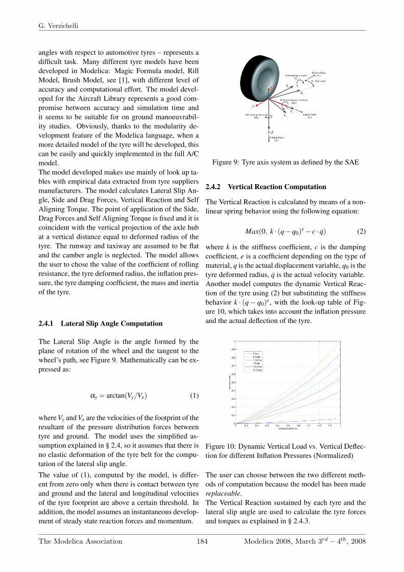
The Lateral Slip Angle is the angle formed by theplane of rotation of the wheel and the tangent to thewheel’s path, see Figure 9. Mathematically can be ex-pressed as:

αy = arctan(Vy/Vx) (1)

where Vy and Vx are the velocities of the footprint of theresultant of the pressure distribution forces betweentyre and ground. The model uses the simplified as-sumption explained in § 2.4, so it assumes that there isno elastic deformation of the tyre belt for the compu-tation of the lateral slip angle.The value of (1), computed by the model, is differ-ent from zero only when there is contact between tyreand ground and the lateral and longitudinal velocitiesof the tyre footprint are above a certain threshold. Inaddition, the model assumes an instantaneous develop-ment of steady state reaction forces and momentum.

Figure 9: Tyre axis system as defined by the SAE

2.4.2 Vertical Reaction Computation

The Vertical Reaction is calculated by means of a non-linear spring behavior using the following equation:

Max(0, k · (q−q0)e − c · q̇) (2)

where k is the stiffness coefficient, c is the dampingcoefficient, e is a coefficient depending on the type ofmaterial, q is the actual displacement variable, q0 is thetyre deformed radius, q̇ is the actual velocity variable.Another model computes the dynamic Vertical Reac-tion of the tyre using (2) but substituting the stiffnessbehavior k · (q− q0)e, with the look-up table of Fig-ure 10, which takes into account the inflation pressureand the actual deflection of the tyre.

Figure 10: Dynamic Vertical Load vs. Vertical Deflec-tion for different Inflation Pressures (Normalized)

The user can choose between the two different meth-ods of computation because the model has been madereplaceable.The Vertical Reaction sustained by each tyre and thelateral slip angle are used to calculate the tyre forcesand torques as explained in § 2.4.3.

G. Verzichelli


2.4.3 Side, Drag Forces and Self Aligning TorqueComputation

The equations which compute the drag and side forcesare as follow:

D = µR ·Fz +D′cos(αy)−S′sin(αy) (3)

S = S′cos(αy)+D′sin(αy) (4)

where µR is the rolling friction coefficient, Fz is theVertical Load, D′ and S′ are the drag and side forcesresolved in the wheel plane reference system and αy isthe slip angle. Notably, there is no need to manipulatethem if αy changes sign, because of the trigonomet-ric functions sin and cos and the shape of the curvesof Figures 11 and 12. Differently, if the A/C changesthe direction of motion, i.e. instead of moving for-ward, moves backward, during push-back manoeuvresfor instance, there is the need to change the sign of theprevious equations. For this reason, the RHS of (3)and (4) is multiplied by (− tanh(τ ·Vx)), where τ is atime constant chosen by the user and the tanh is used toassure a smooth transition around zero (the A/C is as-sumed to move forward when Vx < 0). The final equa-tions are:

D = [µ ·Fz +D′cos(αy)−S′sin(αy)] · [− tanh(τ ·Vx)]

S = [S′cos(αy)+D′sin(αy)] · [− tanh(τ ·Vx)]

The torque developed by the Self Aligning Torque canbe simply computed using the look-up table of Fig-ure 13. A snapshot of the tyre model in Dymola isgiven in Figure 14.

Figure 11: Drag Force vs. Slip Angle for differentVertical Load (Normalized)

Figure 12: Side Force vs. Slip Angle for different Ver-tical Load (Normalized)

Figure 13: Self Aligning Torque vs. Slip Angle fordifferent Vertical Load (Normalized)

2.5 Engine Model

The Engine Model is simply represented by a PIDController. The user can define the desired steady statevelocity and the spool time: the engine forces changeaccordingly to maintain the value of the demanded ve-locity. In fact during a turn, the A/C speed tends to de-cay because of the development of the centripetal forceat the tyre contact footprint which counterbalances thecentrifugal force. The user can also decide when toswitch the engine on (T hrust 6= 0) or off (T hrust = 0)due to conditions linked either to time-based events orboolean-based events. Furthermore, in order to simu-late an instantaneous loss of thrust, due for instance toan engine failure for the simulation of a rejected take-off case, the TriggeredMax block is used. It samplesthe continuous input signal whenever the trigger inputsignal is rising (i.e., trigger changes from false to true).The maximum, absolute value of the input signal (En-gine Thrust) at the sampling point is provided as out-put signal. So the Thrust on the remaining functioningengines is assumed to be constant and its value equal



Figure 14: Tyre Model in Dymola

to the one at the instant when the failure occurred.

2.6 Aerodynamic Model

The Aerodynamic forces and momenta are lumped atthe CG location. The equations used are as follows:

FxA =12

ρV 2CGS Cx

FyA =12

ρV 2CGS Cy

FzA =12

ρV 2CGS Cz (5)

MxA =12

ρV 2CGS b Cl

MyA =12

ρV 2CGS c̄ Cm

MzA =12

ρV 2CGS b Cn

where S is the wing wet area, b the wing span, and c̄ themean aerodynamic chord. These equations are multi-plied with a positive or negative sign to account forthe axes reference system. The computation of someof the angles necessary for the evaluation of the coef-ficients of (5) is as follow:

α = arctan( u

w

)β = arcsin

(v

|VCG|

)

Other angles and their rate of change are computed us-ing a similar approach.The rotation of the Rudder is taken into account sep-arately using the look-up table of Figure 15. It is as-sumed that the rudder has full authority when its ro-tation reaches 30◦, and it increases linearly from zeroto 30◦. The rotation of the rudder implies also a rota-tion of the nose wheel, this has been implemented inthe Steering Laws in the Monitoring and CommandingModel.

Figure 15: Rudder Force at 30◦ Rotation vs. A/CSpeed (Normalized)

2.7 Hydraulics Steering System Model

The Hydraulics Steering System Model consists of aNose Wheel Steering (NWS) and a BWS system. Forthe first one the kinematics of the actuation consists ofa push-pull actuator arrangement which is capable tosteer the A/C from a straight ahead position (θNWS =0 deg) to a full powered steering rotation of the NoseWheel (θNWS = ±θNWSmax). For the second one, thekinematics consist of a single linear actuator, whichsteers the BWS accordingly to the actual position ofthe NWS angle and ground speed of the A/C (θBWS =f (θNWS, GSA/C)). An overview of the NWS and BWSSteering System models is given hereafter.

2.7.1 NWS Hydraulics Steering System Model

At the top-level, the system briefly consists of a Nor-mal Selector Valve Manifold (NSELVM), an AlternateSelector Valve Manifold (ASELVM), a Local Electro-hydraulic Generation System (LHEGS), Nose Land-ing Gear (NLG) Shutoff-Swivel Valve, an HydraulicControl Block (HCB), a servo-valve electro-hydraulicNWS, two Change Over Valves and two steering actu-ators. In addition, the system is connected to the hy-draulic power distribution system via the High Pres-sure (≈ 350 bar) and Low Pressure Manifolds (≈5 bar). All the electrical signals necessary to ener-gize and de-energize the various selector valves andcommand the servo-valve are sent by/to COM/MONto the Hydraulics System. In turn, the latter trans-mits all the signal necessary to monitor the systemto COM/MON, for instance the value of the pressuredownstream NSELVM, via Pressure Transducer (PT)PT4.In the model, all the previous elements have been mod-eled, except the ASELVM and the LHEGS, which are

G. Verzichelli


mainly necessary only if particular faults in the systemoccur (Reversion from Normal to Alternate Mode) andthey will be modeled in the future, see Figure 16.

Figure 16: NWS Hydraulics Steering System Modelin Dymola

The model of COM/MON does not pretend to be ex-haustive nor representative of the whole COM/MONsystem, its principal task is to support the functioningof the Hydraulics System Model. The Model has beenbuilt keeping a net interface between the hydraulic do-main, the mechanical domain and the avionic domain:the green flanges represent the interface with the at-tachment points of the mechanical steering actuatorsand the blue and purple signals the interface with theavionic domain, see Figure 16.

The position of the spool of the servo-valve is con-trolled by a PI controller which modulates the cur-rent in order to minimize the error between NWScommanded angle (θNWScom) and actual NWS angle(θNWS). The position of the servo-valve spool allowsthe hydraulic flow to differentially pressurize the fourchambers (Left and Right, Annulus and Full Bore) ofthe steering actuators, so to create push or pull forceson the pistons ends.The attachment points of the actuators are fixed: tothe stationary flange for the cylinders and to the rotat-ing sleeve for the pistons, respectively. This, and theirposition with respect to the upper strut of the shockabsorber, are such to create a steering torque, which istransmitted, via the torque links, to the bottom of theshock absorber strut (piston fork) allowing the A/C tosteer, see Figures 17, 18 and 19.Of particular interest is the situation when one of thetwo actuators stalls: the line of action of the hydraulicforce intersects the axle of rotation of the strut, creat-ing no moment arm. The angle at which this happensis called Change Over Angle (θCOV ), and it is equal to:

θCOV = θ0 − arctan(Fry/Frx)

with θ0 being the angle between the x axis of the noselanding gear reference frame and the vector SrON, Frx

and Fry equal to the x and y coordinates of Fr. Thesecoordinates given in a reference system with the x− yplane orthogonal to the strut axle (if the rake angle isdifferent from zero).

Figure 17: Actuators-rotary sleeve assembly

When θNWS = ±θCOV , one of the two Change OverValve receives the command to change its position, seeFigure 16, either the left or the right one dependingif the A/C is performing a clockwise turn or counter-clockwise turn, so that the corresponding actuator be-gins to push or pull and viceversa.

2.7.2 BWS Hydraulics Steering System Model

At the top-level, the system briefly consists of a Steer-ing Selector Valve Manifold (SSELVM), a left andright BWS Hydraulic Control Block including Selec-tor Valves and Steering Actuator, a left and right lockactuator, a left and right BWS electro-hydraulic servo-vale, an High Pressure supply line (HP) and Low Pres-sure supply line (LP) Manifolds and ATA 29 Electro-Motor Pump (EMP), see Figure 20.Whilst the steering functions of the BWS is similar tothe NWS, except the fact that there is one linear steer-ing actuator per side, the additional challenge has beenin modelling the lock/un-lock mechanism and un-lockactuator, as already explained in § 2.3.1, see Figure 8.

2.8 Monitoring and Commanding Model

The Monitoring and Commanding Model developed atthis stage has the main purpose of allowing the correctfunctioning of the hydraulic and mechanical Model.



Figure 18: NLG Model with Actuators-rotary sleeveassembly in Dymola

The signals to energize or de-energize the several se-lector valves are sent accordingly to the actual condi-tions of the A/C, so to create a closed loop between themain three domains. The implementation of the Steer-ing Laws has been also developed in this model, seefor instance the command of the BWS angle in accor-dance with the actual NWS angle, Figure 21.A more comprehensive model will be developed in asecond stage: in doing that, an extensive use of theStaeGraph Library will be pursued.

3 Simulation Results

The following sections highlight the Dymola set upused to run simulations and the results obtained froma simulation of a Rejected Take Off (RTO) scenario.

3.1 Simulation Settings

The type of integration algorithm used depended uponthe model that was tested. In the case of pure mechan-ical model, the Dassl or the Lsodar algorithms per-formed in an excellent manner. When it came to sim-ulate the full model, combining avionic, hydraulic andmechanical domains, the best performance has beenachieved using the Sdirk34hw method. Notably, theincrease of tolerance of the integrator did not improve

Figure 19: NLG driven by hydraulics actuators at 70◦

with side, drag and vertical forces (blue) and self-aligning torque (green) in Dymola

Figure 20: BWS Hydraulics Steering System Modelin Dymola

the simulation time: as explained in [2], a condition ofoptimum should exists, in the case of the full modela tolerance of 10−5 was used. Quite challenging hasbeen the identification of the right initial conditions:Dymola by default, assigns arbitrary values for the ini-tial conditions of certain variables. The assumptionmade by the software should always be validated bythe user. In the case of the full A/C model, at the begin-ning of the simulation, there are many events that oc-cur: the A/C is settling down on the soil (impact forcedifferent from zero and the shock absorber starts to becompressed), the A/C speed begins to reach the steadystate value, and especially, the hydraulic circuit tendsto find the steady state condition. All this could bequite time consuming from a simulation point of view.Ideally the user should try to find the value of the vari-ables in the steady state condition which would liketo use as starting point of his/her investigation, recordthose values, and use them as initial conditions for allthe following simulations. When this is done, he/she

G. Verzichelli


Figure 21: BWS Steering Laws

could simulate the model up to the steady state con-dition and then used this final condition, as a startingpoint for a new simulation. This method can be usedonly if the model has reached an high level of maturityand many changes are no longer necessary.

3.2 RTO simulation test

The test has been carried out with the following pre-conditions and assumptions: A/C speed at the instantof the left outer engine failure equal to 130 kt, massequal to 560 t, CG position equal to 37.5 %, rollingfriction coefficient µR, equal to 6 e−3, all the steeringcontrollers active, (θNWScom = 0) with no pilots correc-tion after engine failure, no aerodynamic forces andrudder force.The main outputs of interest are the trajectory of thenose and CG, Figures 23 and 24, A/C heading ψ , Fig-ure 27; A/C CG lateral linear and angular accelera-tions, ayCG and ω̇zCG respectively, Figures 25 and 26.Notably, It takes 1.25 s before the CG linear acceler-ation along y direction starts to become negative, seeFigure 25, in fact the CG first moves towards the pos-itive x− z half plane and then after a while, it starts tomove towards the negative x− z half plane, followingthe nose. After three seconds from the instant of thesimulated engine failure, the nose has moved of circa37.22 cm towards the left.

4 Future Work

The future work will be mainly based on the enhance-ment of the Aircraft Library with the development ofmore comprehensive models and new models as well;on the investigation of Modelica capability to producecode to run models in a Real Time environment forhybrid simulations on the landing gear test rig and, fi-nally, on the validation of the models with Flight Test

Figure 22: Snapshot of the A/C, five seconds after aleft outer engine failure with highlighted CG trajectory(in blue)

Figure 23: CG and Nose trajectory (engine failure atx = −382.47 m. A/C moves forward when x < 0)

and Test Rig Data.

5 Conclusions

Though the work presented in this paper is one of thefirst large-scale application of Modelica for the simu-lation of landing gears and aircrafts, its findings madeclear the power and potentiality of the language tomodel and simulate so tightly coupled systems suchthe ones which equip new modern airplanes.The fact that the source code is completely open to theuser implies a huge potentiality to increase the level ofaccuracy of every model component/assembly/system.The acasuality feature of the language implies a realopportunity to develop a re-usable library of modelswhich is not truly possible with models built with a ca-sual language. Furthermore, the system modeled withModelica provides a unique feature which is the ca-pability of the model to look like the real system un-dergoing the design process: in a large enterprise this



Figure 24: CG and Nose trajectory (engine failure atx = −382.47 m. A/C moves forward when x < 0)(Magnified)

Figure 25: A/C linear acceleration along y at CG loca-tion (Magnified)

represents a point of convergence between designersand modelers. No particular skills are necessary to beable to read the model which faithfully should repre-sent the system, so that feedbacks, critics, enhance-ments, approvals can be easily agreed between severalactors not necessarily experts of modelling and simu-lations techniques, even before any type of simulationis performed.

If Modelica is used in a large industrial environmentsome enhancements are advisable, though these issuesmay not be necessarily attributable to Modelica itself:the capability of creating geometry (with mass, iner-tia, CG location and surface shape information) di-rectly from a Computer-Aided Drawing (CAD) soft-ware in an automated manner; a flexible body sim-ulation capability, including contacts and conditionalconnection/dis-connection of bodies/joints during thesame simulation.

Figure 26: A/C angular acceleration along z at CG lo-cation

Figure 27: A/C heading angle ψ

6 Acknowledgments

The Author would like to acknowledge Airbus for giv-ing the opportunity to attend the Modelica 2008 Con-ference and present this work, Mr. Sanjiv Sharma forthe continuous support and for reviewing the paper,Miss. Serena Simoni for having accepted the chal-lenge of learning Modelica and Dymola and startedthis work and finally Claytex Services Limited andDynasym AB for solving technical issues related tothe use of the software.

Acronyms

A/C Aircraft

ASELVM Alternate Selector Valve Manifold

BLG Body Landing Gear

BWS Body Wheel Steering

CAD Computer-Aided Drawing

G. Verzichelli


Figure 28: A/C demanded and actual speed [m/s]

Figure 29: A/C demanded and actual speed [m/s](Magnified)

CG Centre of Gravity

EMP ATA 29 Electro-Motor Pump

GUI Graphical User Interface

HCB Hydraulic Control Block

HP High Pressure supply line

LHEGS Local Electro-hydraulic Generation System

LP Low Pressure supply line

MAC Mean Aerodynamic Chord

NLG Nose Landing Gear

NSELVM Normal Selector Valve Manifold

NWS Nose Wheel Steering

PT Pressure Transducer

RTO Rejected Take Off

References

[1] M. Beckman and J. Andreasson. Wheel modellibrary for use in vehicle dynamics studies. KTHVehicle Dynamics, [email protected]

[2] C. Clauβ and P. Beater. Electronic, Hydraulic,and Mechanical Subsystems of a Universal Test-ing Machine Modeled with Modelica. 2nd Inter-national Modelica Conference, Proceedings, pp.25-30, Germany



development of an aircraft and landing gears model with ... · development of an aircraft and...

Documents