development of a preliminary cost estimation

DEVELOPMENT OF A PRELIMINARY COST ESTIMATION METHOD FOR

WATER TREATMENT PLANTS

By

JWALA RAJ SHARMA

Presented to the Faculty of the Graduate School of

The University of Texas at Arlington in

Partial Fulfillment of Requirements

for the Degree of

MASTER OF SCIENCE IN CIVIL ENGINEERING

THE UNIVERSITY OF TEXAS AT ARLINGTON

MAY 2010

iii

ACKNOWLEDGEMENTS

I wish to express my appreciation for Dr. Mohammad Najafi, Ph.D., P.E., Director of Center for

Underground Research and Education (CUIRE) and Assistant Professor, The University of Texas at

Arlington, for his continuous and invaluable guidance, support, and encouragement during my graduate

studies, and research works. It has been a pleasure working under him in various research projects

including this thesis.

I wish to thank Dr. Syed R. Qasim, Professor Emeritus, for his special guidance during the

research project which this thesis report is based on.

I wish to acknowledge the members of my graduate committee, Dr. Melanie L. Sattler, P.E., and

Dr. Hyeok Choi for serving on my committee and their review and suggestions for improvement of the

thesis report.

A special thanks to my father Murali Prasad Sharma, and mother Geeta Sharma, to whom this

thesis report is dedicated. Lastly, I wish to thank my wife, Srishti Pathak, for her love, support, and

patience throughout my graduate work.

March 25, 2010

iv

ABSTRACT

DEVELOPMENT OF A PRELIMINARY COST ESTIMATION METHOD FOR

WATER TREATMENT PLANTS

Jwala Raj Sharma, M.S.

The University of Texas at Arlington, 2010

Supervising Professor: Dr. Mohammad Najafi

Reliable cost estimates for construction, and operation and maintenance (O&M) of water

treatment plants are essential for their project planning and design. During the planning phases of the

project, preliminary cost estimates are developed for major project components, and for screening of

alternatives.

Construction and O&M cost curves are widely used for developing preliminary cost estimates.

This method is time consuming and there is possibility of human errors. Therefore, for this thesis,

construction, and O&M cost equations were developed considering historical cost data for different unit

operations and processes involved in a water treatment plant. These equations were developed from

historical cost data and can be used to develop preliminary cost estimate for different alternative process

trains of a water treatment project. The historical cost data were updated to September 2009 costs by

using Engineering News Record (ENR) and Bureau of Labor Statistics (BLS) cost indexes, and

September 2009 prices of energy and labor.

Use of single cost index to further update construction and O&M costs provides a simple and

straight forward method for future cost updating using ENR construction and building cost indexes.

v

TABLE OF CONTENTS

ACKNOWLEDGEMENTS ............................................................................................................................. iii

ABSTRACT .................................................................................................................................................. iv

LIST OF ILLUSTRATIONS .......................................................................................................................... vii

LIST OF TABLES ......................................................................................................................................... ix

Chapter Page

1 INTRODUCTION ........................................................................................................................................ 1

1.1 Background ......................................................................................................................................... 1

1.2 Need Statement .................................................................................................................................. 2

1.3 Objectives ........................................................................................................................................... 3

1.4 Methodology ....................................................................................................................................... 3

1.5 Thesis Organization ............................................................................................................................ 3

1.6 Expected Outcome ............................................................................................................................. 4

1.7 Chapter Summary ............................................................................................................................... 4

2 LITERATURE REVIEW .............................................................................................................................. 5

2.1 Introduction ......................................................................................................................................... 5

2.2 Water Treatment Plants and Their Processes .................................................................................... 5

2.2.1 Water Quality ............................................................................................................................... 5

2.2.2 Water Treatment System ............................................................................................................ 6

2.2.3 Unit Operations and Processes................................................................................................... 7

2.3 Water Treatment Plant Cost Data .................................................................................................... 23

2.4 Equation Generation ......................................................................................................................... 23

2.5 Cost Update ...................................................................................................................................... 24

2.5.1 The Engineering News Record (ENR) Indexes ......................................................................... 25

2.5.2 Indexes Applicable for Update of Cost ...................................................................................... 26

2.5.3 Bureau of Labor Statistics (BLS) Indexes ................................................................................. 26

2.6 Present worth and annual equivalent worth calculation ................................................................... 27

2.7 Chapter Summary ............................................................................................................................. 28

3 METHODOLOGY ..................................................................................................................................... 29

3.1 Introduction ....................................................................................................................................... 29

3.2 Comparison of Cost Update Methods .............................................................................................. 29

vi

3.2.1 Single Index ............................................................................................................................... 29

3.2.2 Multiple Indexes ........................................................................................................................ 29

3.2.3 Controlled Single Index ............................................................................................................. 29

3.3 Update of Construction and O&M Cost Data.................................................................................... 30

3.4 Development of Cost Equations ....................................................................................................... 31

3.5 Use of Microsoft Excel™ for Regression Analysis ........................................................................... 31

3.6 Excel™ Template to Prepare Preliminary Cost Estimate of Water Treatment Plant ....................... 32

3.7 Chapter Summary ............................................................................................................................. 33

4 RESEARCH RESULTS ............................................................................................................................ 34

4.1 Introduction ....................................................................................................................................... 34

4.2 Comparison of Cost Update Methods .............................................................................................. 34

4.3 Generalized Construction Cost Equations ........................................................................................ 34

4.3.1 Generalized Operation and Maintenance Cost Equations ........................................................ 37

4.4 Illustration.......................................................................................................................................... 59

4.5 Excel™ Template for Preliminary Cost Estimate of 1 mgd to 200 mgd Water Treatment Plants .... 61

4.5.1 Project Details ........................................................................................................................... 61

4.5.2 Unit Operation and Processes .................................................................................................. 62

4.5.3 Summary of Capital Costs ......................................................................................................... 62

4.5.4 Summary of O&M Costs ............................................................................................................ 62

4.5.5 Present & Annual Value ............................................................................................................ 62

4.6 Chapter Summary ............................................................................................................................. 63

5 CONCLUSIONS AND RECOMMENDATIONS........................................................................................ 64

5.1 Conclusions ...................................................................................................................................... 64

5.2 Recommendations for Future Research ........................................................................................... 64

APPENDIX

A. COST AND LOCATION INDEXES FOR THE UNITED STATES .......................................................... 66

B. CONTROLLED SINGLE INDEX UPDATES AT INTERVAL OF 8 AND 10 YEARS .............................. 76

C. COST BASIS FOR WATER TREATMENT UNIT OPERATIONS AND PROCESSES .......................... 82

D. LIST OF ABBREVIATIONS .................................................................................................................... 95

REFERENCES ............................................................................................................................................ 98

BIOGRAPHICAL INFORMATION ............................................................................................................. 101

vii

LIST OF ILLUSTRATIONS

Figure Page

1.1 Components of Capital, and Operation and Maintenance Costs ..................................................... 2

2.1 Alternative Unit Operations and Processes for Different Stages of Residual Management .......... 21

3.1 Flow Chart for Forward Method ...................................................................................................... 31

3.2 Sample Equation Generation Chart from Excel™ .......................................................................... 32

4.1 Comparison of Updated Construction Costs of Chlorine Storage and Feed System .................... 35

4.2 Comparison of Updated Construction Costs of Liquid Alum Feed System .................................... 35

4.3 Comparison of Updated Construction Costs of Rectangular Clarifier ............................................ 36

4.4 Comparison of Updated Construction Costs of Gravity Filtration Structures ................................. 36

4.5 Comparison of Updated Construction Costs of Gravity Filtration Structures ................................. 37

B.1 Construction Costs of 3600 ft2 Rectangular Clarifier, Updated Using Single Index, Multiple Indexes, and Controlled Single Index, 8 yr Interval ................................ 77

B.2 Construction Costs of 50 mgd Gravity Filtration Structure, Updated Using Single Index, Multiple Indexes, and Controlled Single Index, 8 yr Interval ................................ 77

B.3 Construction Costs of 540 lb/hr Capacity Liquid Alum Feed System, Updated Using Single Index, Multiple Indexes, and Controlled Single Index, 8 yr Interval ................................ 78

B.4 Construction Costs of 2000 lb/day Chlorine Storage and Feed System, Updated Using Single Index, Multiple Indexes and Controlled Single Index, 8 yr Interval ................................. 78

B.5 Construction Costs of 1400 ft2 Filter Area Capacity Air-Water Backwash, Updated Using Single Index, Multiple Indexes, and Controlled Single Index, 8 yr Interval ................................ 79

B.6 Construction Costs of 3600 ft2 Rectangular Clarifier, Updated Using Single Index, Multiple Indexes, and Controlled Single Index, 10 yr Interval .................................................... 79

B.7 Construction Costs of 50 mgd Gravity Filtration Structure, Updated Using Single Index, Multiple Indexes, and Controlled Single Index, 10 yr Interval .................................................... 80

B.8 Construction Costs of 540 lb/hr Capacity Liquid Alum Feed System, Updated Using Single Index, Multiple Indexes, and Controlled Single Index, 10 yr Interval .............................. 80

B.9 Construction Costs of 2000 lb/day Chlorine Storage and Feed System, Updated Using Single Index, Multiple Indexes and Controlled Single Index, 10 yr Interval ............................... 81

viii

B.10 Construction Costs of 1400 ft2 Filter Area Capacity Air-Water Backwash, Updated Using Single Index, Multiple Indexes, and Controlled Single Index ..................................................... 81

ix

LIST OF TABLES

Table Page

2.1 Summary of Various Unit Operations and Processes ...................................................................... 6

2.2 Selection Guide for Some Basic Types of Clarifiers ...................................................................... 12

2.3 Types of Filter Medium and Applications ....................................................................................... 14

2.4 Advantages and Disadvantages of Different Types of Backwash System .................................... 16

2.5 Features of Membrane Processes and Ion Exchange ................................................................... 17

2.6 General Advantages and Disadvantages of Water Treatment Oxidants ....................................... 19

2.7 Descriptions and Applications of Different Stages of Residual Management and Their Alternatives ................................................................................................................. 22

2.8 Cost Components and Applicable Index for Construction and Operation & Maintenance Costs of Water Treatment Plants ............................................................................................... 26

2.9 October 1978, Modified October 1978 and September 2009 Index Values .................................. 27

4.1 Generalized Construction Cost Equations Applicable for 1 to 200 mgd Water Treatment Plants .............................................................................................................. 38

4.2 Generalized Construction Cost Equations Applicable for 2,500 gpd to 1 mgd Water Treatment Plants .............................................................................................................. 47

4.3 Generalized O&M Cost Equations Applicable to 1 mgd to 200 mgd Water Treatment Plants .............................................................................................................. 50

4.4 Generalized O&M Cost Equations Applicable for 2,500 gpd to 1 mgd Water Treatment Plants .............................................................................................................. 56

A.1 Cost and Location Indexes for the United States........................................................................... 67

C.1 Cost Basis for Water Treatment Unit Operations and Processes ................................................. 83

1

CHAPTER 1

INTRODUCTION

This chapter presents a brief introduction to cost estimation for construction, and operation and

maintenance (O&M) of water treatment plants and their importance in evaluation of project feasibility.

1.1 Background

Capital and O&M costs of water treatment plants are essential for planning and design of the

treatment facilities. These costs are used to evaluate the financial and economic benefits of the project.

Additionally, these costs are essential for evaluation and comparison of cost and benefits of different

alternatives to select the most feasible alternative.

Water treatment plants utilize many treatment units to achieve a desired degree of treatment. The

collective arrangement of treatment processes are called process diagram, process train or flow

schematic. Many process trains can be assembled from different processes to achieve a desired level of

treatment. However, the most preferred process train is the one that is most cost effective. Many

guidelines have been developed that may assist planners and engineers for evaluation and selection of

cost-effective process diagram.

Cost estimating is defined as the process of prediction of the cost of performing the work within

the scope of the project (Holm et al., 2005). The accuracy of the estimate depends upon how well the

variables and uncertainties within the scope of the project are defined and understood. The construction

and O&M costs of any water treatment project are best developed using detailed engineering cost

estimates. Various components of the capital and O&M costs are shown in Figure 1.1. The cost

components are based on actual quantities of material and manufacturers’ data on the equipment. Such

cost estimates are feasible only after the project design is nearing the final steps and the engineering

plans and specifications are fully developed. However, during the early planning phases of the project

2

when alternative selection and project design are in conceptual stages, preliminary cost estimates

constitute valuable data source for decision making.

Figure 1.1: Components of Capital, and Operation and Maintenance Costs

Historically, alternative but less reliable preliminary cost estimates of treatment units were made

from many published cost curves. These curves have been traditionally developed by U.S. Environmental

Protection Agency (USEPA), public utilities and consulting engineers. Later, Qasim et al. (1992)

developed mathematical equations from the cost curves that simplified the preliminary cost estimating of

capital and O&M costs of treatment units. U.S. Bureau of Reclamation developed computer programs that

integrate the cost equations and provide preliminary cost estimates.

1.2 Need Statement

Developing preliminary cost data from cost curves is time consuming and is subject to human

error in reading the graphical coordinates. Cost equations are more convenient and accurate. Also, these

equations can easily be integrated in a computer program to develop design and cost estimates of the

treatment units. Most challenging task however is updating historical costs into current dollar. The

historical capital and O&M cost estimates utilize combination of indexes provided by Engineering News

Record (ENR) and Bureau of Labor Statistics (BLS) for different cost components of the treatment

Capital Costs O&M Costs

Site preparation and earthwork

Structure

Pipelines

Equipment and installation

Electrical, mechanical and instrumentation

Energy

Parts and Materials

Labor

Site improvement and project closure

3

processes. Over the past forty years BLS has changed bases for cost indexing several times. As a result,

updating costs using the BLS index is more complicated than using ENR indexes.

There is a need to develop a simplified and widely used method to develop and update the capital

and O&M costs. Microsoft Excel™ is a popular and widely used computer spreadsheet program. It offers

a great deal of flexibility and accuracy to develop generalized capital and O&M cost equations. Likewise,

ENR indexes have been traditionally used for cost updating for most infrastructures. To utilize only ENR

indexes for cost updating will offer simplicity and effectiveness in capital cost updating to current dollars.

1.3 Objectives

The objectives of this research are (i) to utilize ENR and BLS indexes to update historical costs to

current costs, (ii) to use a common software tool such as utilize Microsoft Excel™ to develop construction

and O&M cost equations for water treatment processes, and (ii) to accord utilization of the most widely

used ENR engineering indexes to further update the costs.

1.4 Methodology

A comprehensive literature search was conducted to identify and review the available material.

The sources searched include government documents and published reports, books, journal articles,

theses and dissertations, and websites. The subjects searched include (i) construction and O&M costs of

water treatment processes, (ii) theory and design of water treatment processes, (iii) procedures to

develop construction and O&M cost equations, and (iv) applicable methods and cost indexes to update

the historical costs in current dollars.

Microsoft Excel™ was utilized to develop construction, and O&M cost equations from data

obtained through comprehensive literature search. An Excel™ template was created for preliminary

construction, and O&M cost estimates of water treatment plants.

1.5 Thesis Organization

Chapter 1 presents introduction to the cost estimation of water treatment plants and introduces

objectives and methodologies of the thesis. Chapter 2 consists of literature review of process description,

existing cost data of water treatment plants, information on developing cost equations, and cost updating

indexes. Chapter 3 contains the methodology for developing cost equations. The construction and O&M

cost equations developed for water treatment processes are truly the results of this study. They are

4

presented separately in Chapter 4. The case study data are also provided in this chapter. Finally, chapter

5 contains the discussion, conclusions and recommendations.

1.6 Expected Outcome

The expected outcome of this research is availability of cost equations of water treatment

processes and indexes for updating capital and operating costs. These equations and cost indexes will

provide a resource for treatment plant designers and planners to compare the preliminary costs of

process trains and select the most cost-effective system. Additionally, these cost equation can be

integrated within the computer program to select and design a most cost effective treatment plant.

A product of this research will also be a computer program which will have capability to generate

and estimate the cost of alternative process trains and select the most cost effective system.

1.7 Chapter Summary

Preliminary construction and O&M cost estimates for water treatment plants are important for

evaluation of project feasibility and arrangement of project funding. Development of reliable data and

estimation technique is necessary. The objectives of this thesis are to address these needs. The research

methodology will consist of comprehensive literature search and use of computer software for

development of cost estimation method.

5

CHAPTER 2

LITERATURE REVIEW

2.1 Introduction

This chapter consists of the review of findings of a comprehensive literature search that was

conducted as a part of this research. The subjects searched include (i) construction and O&M costs of

water treatment processes, (ii) theory and design of water treatment processes, (iii) procedures to

develop construction and O&M cost equations, and (iv) applicable methods and cost indexes to update

the historical costs in current dollars. Procedures to develop cost equations and applicable indexes will be

reviewed in this chapter.

2.2 Water Treatment Plants and Their Processes

2.2.1 Water Quality

Water in its pure state is a colorless, odorless and tasteless liquid. But, it is able to dissolve most

minerals and can carry other inorganic and inorganic compounds as well as microorganisms in

suspended and/or dissolved form. Thus, water in its natural form mostly contains impurities.

Principal inorganic ions found in most natural water are calcium, magnesium, sodium, potassium,

iron, manganese, carbonate-bicarbonate, chloride, sulfate, nitrate, phosphate and fluoride. There may

also be other minor inorganic ions present in water depending upon the source path of the water. Right

doses of most of these inorganic ions, especially minerals like calcium, magnesium, sodium, potassium,

iron, etc., are essential for human life while other inorganic ions and overdoses of essential inorganic ions

may be toxic to humans. Alkalinity, hardness, total dissolved solids, conductivity, dissolved oxygen,

turbidity, particle count, sodium adsorption ratio and stability of water are indicators for quality and

quantity of inorganic impurities in water.

Organic contaminants present in natural water may be natural organic matter or synthetic

inorganic compounds. Natural organic matters are mainly proteins, carbohydrates and lipids originated

from plant and animal residues. Humification of these substances produces a variety of chemical groups

like hydroxyl, carboxyl, methoxyl and quinoid. Principal synthetic organic compounds that may be found in

6

natural water are surfactants, pesticides and herbicides, cleaning solvents, polychlorinated biphenyls and

disinfection by-products. BOD5, COD, TOC, TOD, ThOD, color, ultraviolet absorbance and fluorescence

are indicators of quality and quantity of organic compounds present in water.

Disease carrying microorganisms like bacteria, viruses, fungi, algae, protozoa and parasitic

worms may be present in raw water.

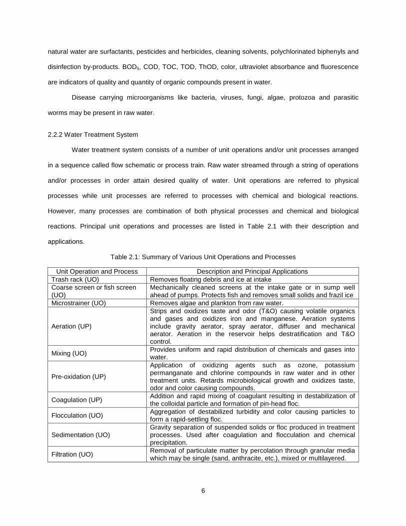
2.2.2 Water Treatment System

Water treatment system consists of a number of unit operations and/or unit processes arranged

in a sequence called flow schematic or process train. Raw water streamed through a string of operations

and/or processes in order attain desired quality of water. Unit operations are referred to physical

processes while unit processes are referred to processes with chemical and biological reactions.

However, many processes are combination of both physical processes and chemical and biological

reactions. Principal unit operations and processes are listed in Table 2.1 with their description and

applications.

Table 2.1: Summary of Various Unit Operations and Processes

Unit Operation and Process Description and Principal Applications Trash rack (UO) Removes floating debris and ice at intake Coarse screen or fish screen (UO)

Mechanically cleaned screens at the intake gate or in sump well ahead of pumps. Protects fish and removes small solids and frazil ice

Microstrainer (UO) Removes algae and plankton from raw water.

Aeration (UP)

Strips and oxidizes taste and odor (T&O) causing volatile organics and gases and oxidizes iron and manganese. Aeration systems include gravity aerator, spray aerator, diffuser and mechanical aerator. Aeration in the reservoir helps destratification and T&O control.

Mixing (UO) Provides uniform and rapid distribution of chemicals and gases into water.

Pre-oxidation (UP)

Application of oxidizing agents such as ozone, potassium permanganate and chlorine compounds in raw water and in other treatment units. Retards microbiological growth and oxidizes taste, odor and color causing compounds.

Coagulation (UP) Addition and rapid mixing of coagulant resulting in destabilization of the colloidal particle and formation of pin-head floc.

Flocculation (UO) Aggregation of destabilized turbidity and color causing particles to form a rapid-settling floc.

Sedimentation (UO) Gravity separation of suspended solids or floc produced in treatment processes. Used after coagulation and flocculation and chemical precipitation.

Filtration (UO) Removal of particulate matter by percolation through granular media which may be single (sand, anthracite, etc.), mixed or multilayered.

7

Table 2.1 - continued

Unit Operation and Process Description and Principal Applications

Chemical precipitation (UP) Addition of chemicals in water to transform dissolved compounds into insoluble matters. Removes hardness, iron and manganese and many heavy metals.

Lime-soda ash (UP) Chemical precipitation process to remove hardness of water by precipitating excess amounts of calcium (Ca) and magnesium (Mg).

Recarbonation (UP) Bubbling of carbon dioxide. Restores chemical balance of water after lime-soda process. Converts supersaturated forms of Ca and Mg into more soluble forms. Lowers pH.

Activated carbon adsorption (UP)

Used as powdered activated carbon (PAC) at the intake or as granular activated carbon (GAC) bed after filtration. Removes T&O causing compounds, chlorinated compounds and many metals.

Activated alumina (UP) Removes species like fluoride, phosphate, arsenic and selenium from water by hydrolytic adsorption.

Disinfection (UP) Achieved by ultraviolet radiation and by oxidative chemicals such as chlorine (most common), bromine, iodine, potassium permanganate and ozone. Kills disease-causing organisms.

Ammoniation (UP) Converts free chlorine residual to chloramines. Chloramines are less reactive and thus have fewer tendencies to combine with organic compounds. Reduces T&O and Trihalomethane (THM) formation.

Fluoridation (UP) Addition of sodium fluoride, sodium silicofluoride and/or hydrofluosilicic acid in finished water. Optimizes fluoride level for control of tooth decay.

Biological Denitrification (UP) Provision of organic source such as ethanol or sugar to act as hydrogen donor (oxygen acceptor) and carbon source for anaerobic reduction of nitrate to gaseous nitrogen.

Demineralization (UP) Achieved by ion exchange, membrane process, distillation and/or freezing. Removes dissolved salts.

Ion exchange (UP) Beds containing cation and anion exchange resins. Removes hardness, nitrate and ammonia by selective resins.

Reverse osmosis (RO) and ultrafiltration (UO)

Passage of high-quality water through semi-permeable membranes. Removes dissolved solids like nitrate and arsenic.

Electro-dialysis (UO) Uses electrical potential to remove cations and anions through ion-selective membranes. De-mineralizes water.

Distillation (UO) Consists of multiple-effect evaporation and condensation and distillation with vapor compression. De-mineralizes water.

Freeze (UO) Consists of freezing of saline water and melting of ice (consisting of pure water) so obtained.

Note: UO = Unit operation; UP = unit process. Source: (Qasim et al., 2000, pp. 35-37)

2.2.3 Unit Operations and Processes

Unit operations consist of physical processes used in treatment of water. Principal unit processes

and their cost bases are described below.

2.2.3.1 Aeration

After removal of some solid particles at intake by physical operations like screens and strainers,

aeration is the first process in a water treatment facility. Aeration is process of bringing water in contact

8

with air or other gases in order to expedite the transfer gas and/or volatile substances in and from water

(Cornwell, 1990). Addition of oxygen and removal of hydrogen sulfide, methane and various volatile

organic and aromatic compounds is achieved by aeration. Aeration reduces concentration of taste and

odor producing substances like hydrogen sulfide and various organic compounds by oxidation. It also

oxidizes iron and magnesium to render them insoluble. As a result of above mentioned oxidations, the

cost of subsequent treatment processes are reduced. (Qasim et al., 2000; ASCE and AWWA, 1990).

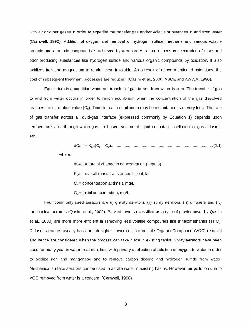
Equilibrium is a condition when net transfer of gas to and from water is zero. The transfer of gas

to and from water occurs in order to reach equilibrium when the concentration of the gas dissolved

reaches the saturation value (Cs). Time to reach equilibrium may be instantaneous or very long. The rate

of gas transfer across a liquid-gas interface (expressed commonly by Equation 1) depends upon

temperature, area through which gas is diffused, volume of liquid in contact, coefficient of gas diffusion,

etc.

dC/dt = KLa(Cs – C0) .......................................................................................... (2.1)

where,

dC/dt = rate of change in concentration (mg/L.s)

KLa = overall mass-transfer coefficient, l/s

Cs = concentration at time t, mg/L

C0 = initial concentration, mg/L

Four commonly used aerators are (i) gravity aerators, (ii) spray aerators, (iii) diffusers and (iv)

mechanical aerators (Qasim et al., 2000). Packed towers (classified as a type of gravity tower by Qasim

et al., 2000) are more more efficient in removing less volatile compounds like trihalomethanes (THM).

Diffused aerators usually has a much higher power cost for Volatile Organic Compound (VOC) removal

and hence are considered when the process can take place in existing tanks. Spray aerators have been

used for many year in water treatment field with primary application of addition of oxygen to water in order

to oxidize iron and manganese and to remove carbon dioxide and hydrogen sulfide from water.

Mechanical surface aerators can be used to aerate water in existing basins. However, air pollution due to

VOC removed from water is a concern. (Cornwell, 1990).

9

2.2.3.2 Coagulation and Flocculation

Water treatment processes require techniques, understanding and input from a wide range of

disciplines including engineering, chemistry, water quality and microbiology (Qasim et al., 2000).

Coagulation and flocculation have different meanings to different people and no unique correct and

universal definitions for these terms exist (Amirtharajah & O'Melia, 1990). ASCE and AWWA, 1990

described coagulation and flocculation as a chemical/physical process of blending or mixing a coagulating

chemical into a stream and then gently stirring the blended mixture in order to improve the particle and

colloid reduction efficiency of subsequent settling and/or filtration process. Similary, according to Qasim et

al., 2000, suspended particles with lower size spectrum do not readily settle and require physical and

chemical conditioning. Coagulation is chemical conditioning of colloids by addition of chemicals that

modify the physical properties of colloids. Flocculation is physical conditioning of colloids by gently mixing

the suspension to accelerate interparticle contact and thus promoting agglomeration of colloidal particles

into larger floc. Whereas, according to Amirtharajah & O'Melia, 1990, coagulation encompasses all

reactions, mechanisms and results in the overall process of particle aggregation within water being

treated. These include in situ coagulant formation, chemical particle destabilization and physical

interparticle contacts. Flocculation is the physical process of producing contacts.

Stable colloids are colloids which do not readily settle. Colloids like ordered structures from soap

and detergent molecules (micelles), proteins, starches large polymers and some humic substances are

stable indefinitely. These colloids are energetically or thermodynamically instable are are termed as

reversible colloids (Amirtharajah & O'Melia, 1990). Colloids that are not stable indifinitely are termed as

irreversible and can be coagulated. The terms stable and unstable for irreversible colloids have kinetic

meaning. Coagulation is used to increase the rate or kinetics at which particles aggregate.

The principal forces occurring between particles are electrostatic forces, van der Waals forces

and hydrodynamic forces or Brownian motion (Amirtharajah & O'Melia, 1990; Qasim et al., 2000). Most of

the colloids present in water are electrically charged. The particles with similar charge repel each other

while the ones with opposite charges attract each other. These forces of attraction and repulsion are

electrostatic forces. The force of attraction between any two mass that depend on mass of the bodies and

10

the distance between them is known as van der Waals forces. Hydrodynamic forces or Brownian motion

is force due to motion of water molecules.

Coagulation involves addition of chemicals into water in order to break down the stabilizing forces

and/or enhance the destabilizing forces. Such chemicals may be metal salts like aluminium sulfate (alum),

ferric sulfate, ferric chloride and ferrous sulfate and/or polymers. These chemicals are known as

coagulants. The processes involved in colloid destabilization are compression of the double layer,

counter-ion adsorption and charge neutralization, interparticle bridging, enmeshment in a precipitate and

hetero-coagulation (Qasim et al, 2000; Amirtharajah & O'Melia, 1990).

Compression of the double layer includes addition of positive (counter) ions to neutralize the

predominant negative charge in colloids. This reduces the electrostatic forces of repulsion between the

similar ions and van der Waals forces become predominant. As a result, floc is formed due to

agglomeration of particles by van der Waals forces of attraction between the particles.

2.2.3.3 Clarification (Sedimentation and Floatation)

Clarification is defined as process of separating suspension into clarified fluid and more

concentrated suspension (Kawamura, 2000). Clarification is widely used after coagulation and flotation

and before filtration in order to reduce load on filtration process (ASCE and AWWA, 1990; Kawamura,

2000; Qasim et al., 2000; Gregory & Zabel, 1990). Sedimentation utilizes gravity settling to remove

suspended solids while floatation utilizes buoyancy for solid-liquid separation (Kawamura, 2000).

Based on criteria of the size, quantity, and specific gravity of the suspended solids to be

separated, Kawamura (2000) classified sedimentation process into grit chamber (plain sedimentation)

and sedimentation tanks (clarifiers). Qasim et al., (2000) and Gregory & Zabel (1990) described four

types or classes of sedimentation: (i) Type I Sedimentation or discrete settling that describes the

sedimentation of low concentrations of particles that settle as individual entities, eg. Silt, sand,

precipitation, etc.; (ii) Type II sedimentation or flocculant settling that describes sedimentation of larger

concentrations of solid that agglomerate as they settle, eg. Coagulant surface waters; (iii) Type III

sedimentation or hindered settling or zone settling that describes sedimentation of a suspension with

solids concentration sufficiently high to cause the particles to settle as a mass, eg. Upper portion of

sludge blanket in sludge thickeners; (iv) Type IV sedimentation or compression settling that describes

11

sedimentation of suspensions with solids concentration so high that the particles are in contact with one

another and further sedimentation can occur only by compression of mass, eg. lower portion of gravity

sludge thickeners.

According to Kawamura (2000), important cinsiderations that directly affect the design of the

sedimentation process are: (i) overall treatment process, (ii) nature of the suspended matter within the

raw water, (iii) settling velocity of the suspended particles to be removed, (iv) local climatic conditions, (v)

raw water characteristics, (vi) geological characteristics of the plant site, (vii) variations in the plant flow

rate, (viii) occurrence of flow short-circuiting within the tank, (ix) type and overall configuration of the

sedimentation tank, (x) design of the tank inlet and outlet, (xi) type and selection of high-rate settling

modules, (xii) method of sludge removal, and (xiii) cost and shape of the tank.

Horizontal flow-type sedimentaion basins are most common in water treatment (ASCE and

AWWA, 1990). Configuration of horizontal flow-type sedimentation basins can be rectangular, multistorey,

circular, and inclined (plate and tube) settlers (Gregory & Zabel, 1990). Other types of clarifiers that are

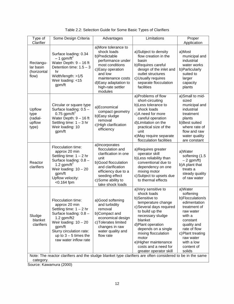
used in water treatment are upflow clarifiers, reactor clarifiers and sludge blanket clarifiers. Some design

criteria, advantages and disadvantages, and proper application of some basic types of clarifiers are listed

in Table 2.2.

In floatation, gas bubbles are attached to solid particles to cause the apparent density of the

bubble-solid agglomerates to be less than that of water, thereby allowing the agglomerate to float to the

surface (Gregory & Zabel, 1990). Three types of flotation are: (i) electrolytic flotation, (ii) dispersed-air

flotation, and (iii) dissolved-air flotation. Types of flotation tanks used are circular tanks, rectangular tanks

and combined flotation and filtration tanks (Gregory & Zabel, 1990).

2.2.3.4 Filtration

The fundamental system in a water treatment process train that removes particulate matter is

filtration (Kawamura, 2000). Although processes like coagulation, flocculation, and sedimentation remove

much of the turbidity causing colloidal materials, further removal of colloidal materials is required in order

to meet public health standards promulgated after the 1986 Safe Drinking Water Act Amendments.

Filtration is commonly utilized to achieve such further colloid removal (Qasim et al., 2000). Filtration can

12

Table 2.2: Selection Guide for Some Basic Types of Clarifiers

Type of Clarifier

Some Design Criteria Advantages Limitations Proper Application

Rectangu-lar basin (horizontal flow)

Surface loading: 0.34 – 1 gpm/ft2

Water Depth: 9 – 16 ft Detention time: 1.5 – 3

hr Width/length: >1/5 Weir loading: <15

gpm/ft

a) More tolerance to shock loads

b) Predictable performance under most conditions

c) Easy operation and low maintenance costs

d) Easy adaptation to high-rate settler modules

a) Subject to density flow creation in the basin

b) Requires careful design of the inlet and outlet structures

c) Usually requires separate flocculation facilities

a) Most municipal and industrial water works

b) Parlicularly suited to larger capacity plants

Upflow type (radial-upflow type)

Circular or square type Surface loading: 0.5 –

0.75 gpm/ft2 Water Depth: 9 – 16 ft Settling time: 1 – 3 hr Weir loading: 10

gpm/ft

a) Economical compact geometry

b) Easy sludge removal

c) High clarification efficiency

a) Problems of flow short-circuiting

b) Less tolerance to shock loads

c) A need for more careful operation

d) Limitation on the practical size of the unit

e) May require separate flocculation facilities

a) Small to mid-sized municipal and industrial treatment plants

b) Best suited where rate of flow and raw water quality are constant

Reactor clarifiers

Flocculation time: approx 20 min

Settling time: 1 – 2 hr Surface loading: 0.8 –

1.2 gpm/ft2 Weir loading: 10 – 20

gpm/ft Upflow velocity:

<0.164 fpm

a) Incorporates flocculation and clarification in one unit

b) Good flocculation and clarification efficiency due to a seeding effect

c) Some ability to take shock loads

a) Requires greater operator skill

b) Less reliability than conventional due to dependency on one mixing motor

c) Subject to upsets due to thermal effects

a) Water softening (1.5 – 2 gpm/ft)

b) A plant that treats a steady quality of raw water

Sludge blanket clarifiers

Flocculation time: approx 20 min

Settling time: 1 – 2 hr Surface loading: 0.8 –

1.2 gpm/ft2 Weir loading: 10 – 20

gpm/ft Slurry circulation rate:

up to 3 – 5 times the raw water inflow rate

a) Good softening and turbidity removal

b) Compact and economical design

c) Tolerates limited changes in raw water quality and flow rate

a) Very sensitive to shock loads

b) Sensitive to temperature change

c) Several days required to build up the necessary sludge blanket

d) Plant operation depends on a single mixing flocculation motor

e) Higher maintenance costs and a need for greater operator skill

a) Water softening

b) Flocculation/sedimentation treatment of raw water with a constant quality and rate of flow

c) Plant treating raw water with a low content of solids

Note: The reactor clarifiers and the sludge blanket type clarifiers are often considered to be in the same category.

Source: Kawamura (2000)

13

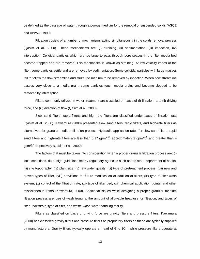
be defined as the passage of water through a porous medium for the removal of suspended solids (ASCE

and AWWA, 1990).

Filtration cosists of a number of mechanisms acting simultaneously in the solids removal process

(Qasim et al., 2000). These mechanisms are: (i) straining, (ii) sedimentation, (iii) impaction, (iv)

interception. Colloidal particles which are too large to pass through pore spaces in the filter media bed

become trapped and are removed. This mechanism is known as straining. At low-velocity zones of the

filter, some particles settle and are removed by sedimentation. Some colloidal particles with large masses

fail to follow the flow streamline and strike the medium to be removed by inpaction. When flow streamline

passes very close to a media grain, some particles touch media grains and become clogged to be

removed by interception.

Filters commonly utilized in water treatment are classified on basis of (i) filtration rate, (ii) driving

force, and (iii) direction of flow (Qasim et al., 2000).

Slow sand filters, rapid filters, and high-rate filters are classified under basis of filtration rate

(Qasim et al., 2000). Kawamura (2000) presented slow sand filters, rapid filters, and high-rate filters as

alternatives for granular medium filtration process. Hydraulic application rates for slow sand filters, rapid

sand filters and high-rate filters are less than 0.17 gpm/ft2, approximately 2 gpm/ft2, and greater than 4

gpm/ft2 respectively (Qasim et al., 2000).

The factors that must be taken into consideration when a proper granular filtration process are: (i)

local conditions, (ii) design guidelines set by regulatory agencies such as the state department of health,

(iii) site topography, (iv) plant size, (v) raw water quality, (vi) type of pretreatment process, (vii) new and

proven types of filter, (viii) provisions for future modification or addition of filters, (ix) type of filter wash

system, (x) control of the filtration rate, (xi) type of filter bed, (xii) chemical application points, and other

miscellaneous items (Kawamura, 2000). Additional issues while designing a proper granular medium

filtration process are: use of wash troughs; the amount of allowable headloss for filtration; and types of

filter underdrain, type of filter, and waste-wash-water handling facility.

Filters as classified on basis of driving force are gravity filters and pressure filters. Kawamura

(2000) has classified gravity filters and pressure filters as proprietory filters as these are typically supplied

by manufacturers. Gravity filters typically operate at head of 6 to 10 ft while pressure filters operate at

14

higher head (Qasim et al., 2000). Gravity filters are used on both small and large water treatment systems

while pressure are typically used in small water treatment systems only because of cost.

Filters as classified on basis of direction of flow can be downflow or upflow. Downflow filters are

most usually used in water treatment system (Qasim et al., 2000).

The solids-holding capacity of the filter bed, the hydraulic loading rate of the filters, and the

finished water quality depend heavily upon the selection of filter media (Qasim et al., 2000). The most

commonly used filter mediums are silica sand and anthracite coal. Other materials that may be used as

filter media are garnet, ilmenite, pumice, and synthetic materials (Kawamura, 2000). On basis of number

of filtration medium used, filters can be categorized as single-medium filters, dual-media filters and mixed-

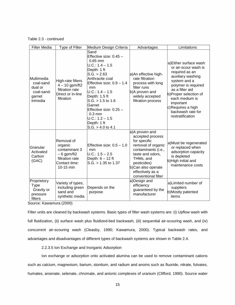
media filters. Different types of filter media and their applications are listed in Table 2.3.

Filters must be cleaned from time to time in order to continue filtration with same efficeincy.

According to (Qasim et al., 2000), filter cell must be cleaned when either (i) the head loss through the

filter exceeds the design value, (ii) turbidity breakthrough causes the effluent quality to be less than a

minimum acceptable level, or (iii) a pre-selected maximum filter run time has passed since it was cleaned.

Table 2.3: Types of Filter Medium and Applications

Filter Media Type of Filter Medium Design Criteria Advantages Limitations

Fine Sand

Slow Sand filter 0.05 – 0.17 gpm/ft2 filtration rate

Effective size: 0.25 – 0.35 mm

U.C.+: 2-3 Depth: 3.3 – 4 ft S.G.* > 2.63

a) Simple design and construction

b) Good effluent quality without pretreatment

a) Requires a large filter bed area

b) Applicable only for good quality area

c) Requires frequent scaping off of surface layer (every 20 – 30 days)

Medium sand

Rapid sand filters 2 – 3 gpm/ft2 filtration rate


U.C.: 1.4 – 1.7 Depth: 2 – 2.5 ft S.G. > 2.63

a) A proven and widely accepted filtration process

b) A wide application range if pretreatment is provided

a) Rather short filter runs due to surface filtration

b) Always a need for coagulation pretreatment and an auxiliary washing system

Coarse sand

High-rate filters 5 – 12 gpm/ft2 filtration rate

Direct filtration


U.C.: 1.4 – 1.7 Depth: 2.6 – 7 ft S.G. > 2.63

a) An effective high-rate filtration process with very long filter runs

b) A wide application range with polymer pretretment.

a) Auxiliary wash system is limited to air-scour type

b) Requires deep filter cells and a special underdrain

15


Filter Media Type of Filter Medium Design Criteria Advantages Limitations

Multimedia coal-sand dual or

coal-sand-garnet trimedia

High-rate filters 4 – 10 gpm/ft2 filtration rate

Direct or in-line filtration

Sand Effective size: 0.45 – 0.65 mm

U.C.: 1.4 – 1.5 Depth: 1 ft S.G. > 2.63 Anthracite coal Effective size: 0.9 – 1.4 mm

U.C.: 1.4 – 1.5 Depth: 1.5 ft S.G. > 1.5 to 1.6 Garnet Effective size: 0.25 – 0.3 mm

U.C.: 1.2 – 1.5 Depth: 1 ft S.G. > 4.0 to 4.1

a) An effective high-rate filtration process with long filter runs

b) A proven and widely accepted filtration process

a) Either surface wash or air-scour wash is required as an auxiliary washing system and a polymer is required as a filter aid

b) Proper selection of each medium is important

c) Requires a high backwash rate for restratification

Granular Activated Carbon (GAC)

Removal of organic contaminant 3 – 6 gpm/ft2 filtration rate

Contact time: 10-15 min


U.C.: 1.5 – 2.5 Depth: 6 – 12 ft S.G. > 1.35 to 1.37

a) A proven and accepted process for specific removal of organic contaminants (i.e., taste and odors, THMs, and pesticides)

b) Can also operate effectively as a conventional filter

a) Must be regenerated or replaced when adsorption capacity is depleted

b) High initial and maintenance costs

Proprietory Type

Gravity or pressure filters

Variety of types, including green sand and synthetic media

Depends on the purpose

a) Design and efficiency guaranteed by the manufacturer

a) Limited number of suppliers

b) Mostly patented items


Filter units are cleaned by backwash systems. Basic types of filter wash systems are: (i) Upflow wash with

full fluidization, (ii) surface wash plus fluidized-bed backwash, (iii) sequential air-scouring wash, and (iv)

concurrent air-scouring wash (Cleasby, 1990; Kawamura, 2000). Typical backwash rates, and

advantages and disadvantages of different types of backwash systems are shown in Table 2.4.

2.2.3.5 Ion Exchange and Inorganic Adsorption

Ion exchange or adsorption onto activated alumina can be used to remove contaminant cations

such as calcium, magnesium, barium, stontium, and radium and anoins such as fluoride, nitrate, fulvates,

humates, arsenate, selenate, chromate, and anionic complexes of uranium (Clifford, 1990). Source water

16

is continually passed through a packed bed of ion-exchange resin bed of ion-exchange resin beds or

alumina granules to achieve ion-exchange. The flow of water may be in upflow or downflow.

Table 2.4: Advantages and Disadvantages of Different Types of Backwash System

Backwash System Typical Backwash Rates Advantages Limitations

Upflow wash with full fluidization

15 to 23 gpm/ft2 a) Restratification of

layers in dual-media.

a) Movement of fine grains to top in rapid sand filters

b) Does not solve all dirty-filter problems.

c) Usually requires auxiliary scour system.

Surface wash plus fluidized-bed backwash

Fixed nozzle system: 2 to 4 gpm/ft2

Rotary nozzle system: 0.5 to 2 gpm/ft2

a) Relatively simple, better cleaning action and lower water requirements.

b) Accessible for maintenance and repair.

a) Rotary type washers sometimes stick in one position temporarily and do not rotate as intended.

b) Mud balls may sink in fluidized beds and no longer come in contact of surface wash jets.

Sequential air-scouring wash

Airflow rate: 3 scfm/ft2 Water flow: 8 to 12 gpm/ft2

a) Interstitial water velocities are increased.

a) Possible loss of filter media.

Concurrent air-scouring wash

For dual-media with about 1.0-mm ES anthracite and 0.5mm ES sand: Airflow rate: 1 to 2 scfm/ft2 Water flow: 5 to 8 gpm/ft2

For sands about 1.00 mm ES: Airflow rate: 2 to 4 scfm/ft2 Water flow: 6 gpm/ft2

For sands about 2.00 mm ES: Airflow rate: 6 to 8 scfm/ft2 Water flow: 6 to 8 gpm/ft2

a) Covers full filter area.

b) Adaptable to any filter dimensions.

c) Agitates entire filter depth.

a) Very limited application. b) Possible loss of filter media. c) Possibility of moving

supporting gravel.

Adapted from Cleasby (1990), Kawamura (2000) and ASCE & AWWA (1990)

The largest application of ion exchange to drinking water treatment has been for softening, i.e.,

removal of calcium, magnesium, and other polyvalent cations in exchange for sodium (Clifford, 1990).

Radium and barium can also be removed during ion softening. Nitrate, arsenate, chromate, and selenate

can be removed by resin beds containing chloride-form anion-exchange resins. Activated alumina is used

to remove fluoride and arsenate. Table 2.5 gives some features of ion exchange process.

2.2.3.6 Membrane processes

Advanced membrane technologies provide superior potable water quality more efficiently than

conventional treatment systems and the depletion of water supplies, saltwater intrusion, and water

pollution, especially by complex organic materials like priority pollutants have contributed to their

17

expanded use (Conlin, 1990). Membrane processes include use of semipermeable membranes to

separate impurities from water.

Table 2.5: Features of Membrane Processes and Ion Exchange

Process Suitable Water Pore/Resin Size

Mol. Wt. Cutoff

(daltons)

Driving Force

Removal Objects Feature

Micro-filtration (MF)

500- µm self-cleaning cartridge filter

0.1-0.2 µm, 0.2 µm is more common

300,000 10-20 psig

Particulates and microbial

Batch process, removal of particles over 0.5 µm

Ultra-filtration (UF)

200 to 500 µm self-cleaning cartridge filter

0.0031-0.01 µm, 0.01 µm is more common

50,000 10-40 psig

Molecular size compounds, particulates and microbial

Batch process, liquid-solid separation

Nano-filtration (NF)

Regular filter effluent or MF filtrate

0.001-0.005 µm

200-400 75-150 psig

NOM, including color, virus, Ca, Mg

Batch process, DBPs control and softening

Reverse Osmosis (RO)

Filtered water, 100- 36,000 mg/L salts

< 1 nm - > 200 psig

Ionized salt ions and colloidal matter

Continuous process, 90-95% inorganic salts and 95-99% organic matter

Electrodialysis (ED)

Filtered water, 500- 8,000 mg/L salts

< 1 nm -

DC*, 0.27-0.36kW/lb salt

Ionized salt ions

Continuous process, incomplete removal of salts

Ion Exchange

Settled or filtered water, 50-1,000 mg/L salts

< 1 nm - < 7 psig

Ionized ions Batch process, complete removal of salts


According to Kawamura (2000), the distinct advantages of of membrane processes over

conventional treatment processes are: (i) removal of suspended solids, with no coagulant, up to about

200 ntu turbidity, (ii) reliable production of good filtered water, (iii) very high “log removal” of Giardia- and

Cryptosporidium- sized particles, (iv) much less space (footprint) required than for the conventional

treatment process, (v) easy integration into the automatic control system, (vi) minimum labor requirement

so that it can maintain unattended operation most of the time, (vii) chemical-free backwash water that can

often be discharged to local water bodies, and (viii) long-term compliance with drinking water regulations.

Kawamura (2000) listed the followings as the shortcomings of membrane processes: (i) membrane

fouling (by bacteria, chlorine residual, and cationic polymer for certain types of membrane), (ii)

18

requirement of treatment of chemically washed waste before disposal, and (iii) need for pretreatment of

poor-quality raw water.

Different types of membrane processes available are: (i) Microfiltration, (ii) Ultrafiltration, (iii)

Nanofiltration, (iv) Reverse osmosis, and (v) Electrodialysis. Diferent features of these membrane

processes are presented in Table 2.5.

2.2.3.7 Chemical Oxidation

Chemical oxidation plays several important roles in water treatment and can be added at several

locations in the treatment process depending upon the purpose of oxidation (Glaze, 1990). Chemical

oxidants are usually added for following purposes: (i) as first stage disinfection, (ii) control of biological

growth in basins, (iii) color removal, (iv) control of tastes and odors, (v) reduction of specific organic

pollutants, (vi) precipitation of metals, (vii) treatment to control growth on filters, (viii) to remove

manganese, and (ix) to provide an extra level of disinfection. Commonly used chemical oxidants are: (i)

Oxygen, (ii) Chlorine, (iii) Chloramines, (iv) Ozone, (v) potassium permanganate, and (vi) Chlorine

dioxide. General advantages and disadvantages of these oxidants are given in Table 2.6.

2.2.3.8 Adsorption of Organic Compounds

Accumulation of a substance (adsorbate) at the interface (adsorbent) between two phases, such

as a liquid and a solid, or a gas and a solid, is called adsorption (Snoeyink, 1990). Primary adsorbent of

organic compounds in water treatment processes is activated carbon. The uses of activated carbon are:

(i) tasteand odor control, (ii) color removal, (iii) removal of mutation causing and toxic substance, and (iv)

removal of THMs. Two primarily used activated carbons in water treatment processes are (i) Powdered

Activated Carbon (PAC), and (ii) Granular Activated Carbon (GAC). Kawamura (2000) listed GAC as a

filter media. Features of GAC as filter media are given in Table 2.3. Advantages of PAC are: (i) low capital

cost, and (ii) ability to change dosage with change in water quality (Snoeyink, 1990). Disadvantages of

PAC include: (i) high operating costs (if high dosage required for long period of time), (ii) inability to

regenerate, (iii) low TOC removal, (iv) difficulty in sludge disposal, and (v) difficulty in complete removal of

PAC particle from finished water.

19

Table 2.6: General Advantages and Disadvantages of Water Treatment Oxidants

Oxidant Advantages Limitations

Chlorine Strong oxidant; Simple feeding; Persistent residual; Long history of use

Chlorinated by-products; Possibility of taste and odor problems; Effectiveness influenced by pH

Chlorimines No THM formation; Persistent residual; Simple feeding; Long history of use

Weak oxidant; Some TOX formation; Possibility of taste, odor, and growth problems

Ozone

Strong oxidant; Usually no THM or TOX formation; No taste or odor problem; Some by-products are biodegradable; Little pH effect; Coagulant aid

Short half-life; On-site generation required; Energy intensive; Complex generation and feeding; Corrosive

Chlorine dioxide Strong oxidant; Relatively persistent residual; No THM formation; No pH effect

TOX formation; ClO3 and ClO2 by-products; On-site generation required; Hydrocarbon odors possible

Potassium permanganate

Easy to feed; No THM formation Pink H2O; Unknown by-products; Causes precipitation

Oxygen Simple feeding; No-by-products; Companion Stripping; Nontoxic

Weak oxidant; Corrosion and scaling

Source: Glaze (1990)

2.2.3.9 Disinfection

Disinfection is a process designed for the deliberate reduction of a number of pathogenic

microorganisms (Haas, 1990). The word “deliberate” and “reduction” are important here because: (i) other

processes like filtration, coagulation and flocculation, etc., also achieve some pathogen reduction but this

is not their primary objective (Haas, 1990), and (ii) total destruction or removal of all organisms is called

sterilization which is not to be confused with disinfection (Kawamura, 2000). Disinfection can be achieved

by chemical oxidation (chemicals involved are discussed above in section g) or ultraviolet (UV) irradiation.

According to Kawamura (2000), major considerations in selecting a disinfection process are: (i)

the presence of surrogate organisms in the drinking water supply, (ii) the feasibility of uding alternative

disinfectants, (iii) the disinfectant residual-contact time relationship, (iv) the formation of disinfectant by-

products and their magnitude, (v) the quality of the process water, (vi) safetly problems associated with

the disinfectants, and (vii) the cost of each disinfection alternative.

2.2.3.10 Water Stability

Tendency of water to either dissolve (corrosion) or deposit (scaling) certain minerals in pipes,

plumbing, and appliance sufaces is known as stability (Qasim et al., 2000). Common method to calculate

stability of water is the Langelier saturation index (LI). Common treatments for corrosive waters are

20

addition of hydrated lime, soda ash or sodium hydroxide. Scale forming waters are commonly treated by

recarbonation.

2.2.3.11 Finished Water Reservoirs (Clearwell)

A clearwell is a storage tank commonly located at a water treatment plant (Qasim et al., 2000).

Four basic purposes of clearwell are: (i) to meet water peak demands, (ii) to provide a sufficient volume of

water for plant operations including filter washing, (iii) to ensure adequate chlorine contact time, and (iv)

to store enough water for firefighting (Kawamura, 2000). Three basic types of clearwells are: (i) ground

level up to approximately 30 ft in height and a steel or reinforced concrete tank, usually cylindrical in

shape, (ii) ground level, a rectangular or square deep basin (25 ft) with a reinforced concrete structure

having vertical sidewalls or a trapezoidal cross section with sidewalls of rather thin concrete and

peripheral walls composed of reinforced concrete that are 8 ft high to support roofing system or anchored

floating membrane cover, and (iii) a rectangular, rather shallow (10 ft) reinforced-concrete tank, located

directly underneath filter structure (Kawamura, 2000). High service pumps may be required for water

distribution (Qasim et al., 2000).

2.2.3.12 Residual Processing and Disposal (Management)

Water treatment processes as discussed above leave behind many residues. A residue is

something remaining after another part has been taken away (Doe, 1990). It is not appropriate to refer all

residues as wastes because some of the residues can be recycled. Residues from water treatment

processes contain organic and inorganic turbidity-causing solids, including algae, bacteria, viruses, silt

and clay, and precipitated chemicals (Qasim et al., 2000). Historically, water treatment residuals were

discharged in natural water bodies. This had major environment implications like aluminium toxicity to

aquatic organisms and so forth (Doe, 1990). Such discharged is now prohibited under the Water Pollution

Control Act Amendments of 1972 and the Clean Water Act of 1977 (Qasim et al., 2000). With these

environmental and legal implications, residual management is one of the major components of any water

treatment facility.

Selection and design of residual management system depends upon quantity of the sludge,

solids content, and the nature of solids. These are primarily a function of treatment processes, added

chemicals, and quality of raw water (Qasim et al., 2000). Some of primary residuals from a water

21

treatment plant are: (i) alum of iron coagulation sludge, (ii) softening sludge, (iii) filter backwash, (iv) iron

and manganese precipitation sludge, (v) residues from coagulant aid, (vi) residues from filter aid, (vii)

spent PAC, (viii) diatomeceous-Earth Filter Washwater, and (ix) spent brine.

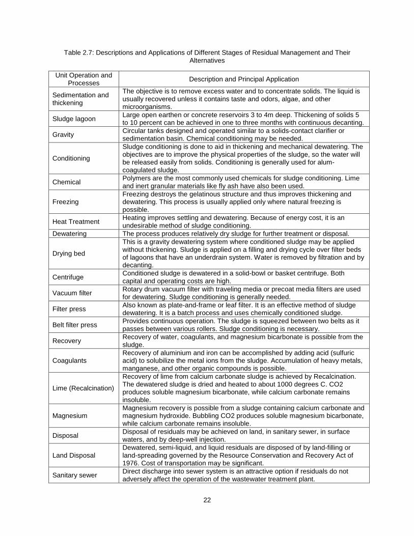
Residual management generally consists of five stages: (i) Thickening, (ii) Conditioning, (iii)

Dewatering, (iv) Recovery, and (v) Ultimate Disposal. Figure 2.1 gives various alternatives for different

stages of residual management. Description and applications of the stages and their alternatives have

been listed in Table 2.7.

Source: Qasim et al. (2000)

2.2.3.13 Instrumentation and Process Control

Modern supervisory control and data acquisition systems can be used to monitor the treatment

plants and distribution systems. The major advantage of computerizing treatment plants is effective

process control through decisions based on timely and accurate information (Kawamura, 2000). There

are six computer systems that are different combinations of the following tasks: (i) report generation, (ii)

data acquisition and logging/report generation/alarm indication, (iii) data acquisition and logging/report

generation/alarm indicator/plant graphic display, (iv) advanced display and data handling: data acquisition

and logging/report generation/alarm indication/plant graphic display/analog variable displays, (v) manual

plant control and advanced data handling: data acquisition and logging/report generation/alarm indication/

Thickening

1. Lagooning 2. Gravity

Thickener 3. Dissolved

Air Flotation

Conditioning

1. Freezing and Thawing

2. Chemical

Dewatering

1. Drying Beds

2. Lagoons 3. Vacuum

Filter 4. Frame

Filter Press

5. Belt Filter Press

6. Centrifuge

Recovery

1. Coagulant

2. Lime 3. Magnesiu

m

Ultimate Disposal

1. Land Disposal

2. Lagooning 3. Land

spreading and Land Filling

4. Discharge into Sanitary Sewer

5. Discharge into Surface Water

6. Deep-well

Figure 2.1: Alternative Unit Operations and Processes for Different Stages of Residual Management

22

Table 2.7: Descriptions and Applications of Different Stages of Residual Management and Their Alternatives

Unit Operation and Processes

Description and Principal Application

Sedimentation and thickening

The objective is to remove excess water and to concentrate solids. The liquid is usually recovered unless it contains taste and odors, algae, and other microorganisms.

Sludge lagoon Large open earthen or concrete reservoirs 3 to 4m deep. Thickening of solids 5 to 10 percent can be achieved in one to three months with continuous decanting.

Gravity Circular tanks designed and operated similar to a solids-contact clarifier or sedimentation basin. Chemical conditioning may be needed.

Conditioning

Sludge conditioning is done to aid in thickening and mechanical dewatering. The objectives are to improve the physical properties of the sludge, so the water will be released easily from solids. Conditioning is generally used for alum-coagulated sludge.

Chemical Polymers are the most commonly used chemicals for sludge conditioning. Lime and inert granular materials like fly ash have also been used.

Freezing Freezing destroys the gelatinous structure and thus improves thickening and dewatering. This process is usually applied only where natural freezing is possible.

Heat Treatment Heating improves settling and dewatering. Because of energy cost, it is an undesirable method of sludge conditioning.

Dewatering The process produces relatively dry sludge for further treatment or disposal.

Drying bed

This is a gravity dewatering system where conditioned sludge may be applied without thickening. Sludge is applied on a filling and drying cycle over filter beds of lagoons that have an underdrain system. Water is removed by filtration and by decanting.

Centrifuge Conditioned sludge is dewatered in a solid-bowl or basket centrifuge. Both capital and operating costs are high.

Vacuum filter Rotary drum vacuum filter with traveling media or precoat media filters are used for dewatering. Sludge conditioning is generally needed.

Filter press Also known as plate-and-frame or leaf filter. It is an effective method of sludge dewatering. It is a batch process and uses chemically conditioned sludge.

Belt filter press Provides continuous operation. The sludge is squeezed between two belts as it passes between various rollers. Sludge conditioning is necessary.

Recovery Recovery of water, coagulants, and magnesium bicarbonate is possible from the sludge.

Coagulants Recovery of aluminium and iron can be accomplished by adding acid (sulfuric acid) to solubilize the metal ions from the sludge. Accumulation of heavy metals, manganese, and other organic compounds is possible.

Lime (Recalcination)

Recovery of lime from calcium carbonate sludge is achieved by Recalcination. The dewatered sludge is dried and heated to about 1000 degrees C. CO2 produces soluble magnesium bicarbonate, while calcium carbonate remains insoluble.

Magnesium Magnesium recovery is possible from a sludge containing calcium carbonate and magnesium hydroxide. Bubbling CO2 produces soluble magnesium bicarbonate, while calcium carbonate remains insoluble.

Disposal Disposal of residuals may be achieved on land, in sanitary sewer, in surface waters, and by deep-well injection.

Land Disposal Dewatered, semi-liquid, and liquid residuals are disposed of by land-filling or land-spreading governed by the Resource Conservation and Recovery Act of 1976. Cost of transportation may be significant.

Sanitary sewer Direct discharge into sewer system is an attractive option if residuals do not adversely affect the operation of the wastewater treatment plant.

23


Unit Operation and Processes

Description and Principal Application

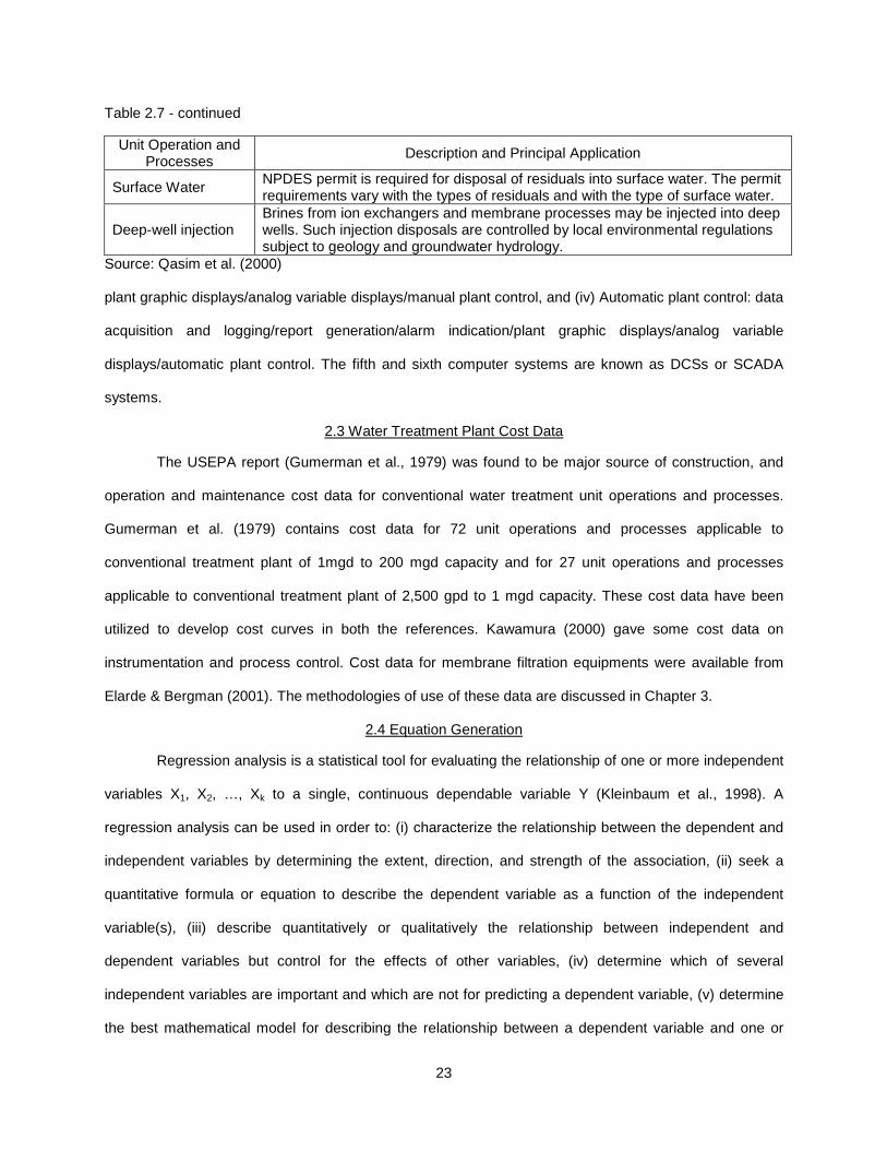
Surface Water NPDES permit is required for disposal of residuals into surface water. The permit requirements vary with the types of residuals and with the type of surface water.

Deep-well injection Brines from ion exchangers and membrane processes may be injected into deep wells. Such injection disposals are controlled by local environmental regulations subject to geology and groundwater hydrology.

Source: Qasim et al. (2000)

plant graphic displays/analog variable displays/manual plant control, and (iv) Automatic plant control: data

acquisition and logging/report generation/alarm indication/plant graphic displays/analog variable

displays/automatic plant control. The fifth and sixth computer systems are known as DCSs or SCADA

systems.

2.3 Water Treatment Plant Cost Data

The USEPA report (Gumerman et al., 1979) was found to be major source of construction, and

operation and maintenance cost data for conventional water treatment unit operations and processes.

Gumerman et al. (1979) contains cost data for 72 unit operations and processes applicable to

conventional treatment plant of 1mgd to 200 mgd capacity and for 27 unit operations and processes

applicable to conventional treatment plant of 2,500 gpd to 1 mgd capacity. These cost data have been

utilized to develop cost curves in both the references. Kawamura (2000) gave some cost data on

instrumentation and process control. Cost data for membrane filtration equipments were available from

Elarde & Bergman (2001). The methodologies of use of these data are discussed in Chapter 3.

2.4 Equation Generation

Regression analysis is a statistical tool for evaluating the relationship of one or more independent

variables X1, X2, …, Xk to a single, continuous dependable variable Y (Kleinbaum et al., 1998). A

regression analysis can be used in order to: (i) characterize the relationship between the dependent and

independent variables by determining the extent, direction, and strength of the association, (ii) seek a

quantitative formula or equation to describe the dependent variable as a function of the independent

variable(s), (iii) describe quantitatively or qualitatively the relationship between independent and

dependent variables but control for the effects of other variables, (iv) determine which of several

independent variables are important and which are not for predicting a dependent variable, (v) determine

the best mathematical model for describing the relationship between a dependent variable and one or

24

more independent variables, (vi) assess the interactive effects of two or more independent variables with

regard to a dependent variable, (vii) compare several derived regression relationships, and (viii) obtain a

valid and precise estimate of one or more regression coefficients from a larger set of regression

coefficients in a given model (Kleinbaum et al., 1998). In this research, regression analysis has been

used to seek a quantitative equation to describe the costs of treatment plants (dependent variable) as a

function of treatment capacity and other parameters like area, feed capacity, etc. (independent variables).

A number of set of observations (estimates in case of this research) can be plotted on a graph to

get a scatter diagram. Basic questions to be dealt with in regression analysis are: (i) what is the most

appropriate mathematical model to use – a straight line, a parabola, a log function, a power function, or

what?, (ii) how to determine the best-fitting model for the data? (Kleinbaum et al., 1998). Common

strategies to tackle first problem are: (i) forward method – begins with simply structured model and adds

more complexity in successive steps, if necessary, (ii) backward method – begins with a complicated

model and successively simplifies it, and (iii) model suggested from experience or theory. Two methods to

solve second question are: (i) least-squares method, and (ii) minimum-variance method. Both these

methods yield same solution (Kleinbaum et al., 1998).

2.5 Cost Update

Order-of-magnitude estimates of projects can be done by making adjustments to cost of similar

project, if available, with respect to variables like time, location and size. These adjustments require

appropriate cost scale-up and location factors. Cost indexes are used to measure a given project to a

basis and typically reference a base year, which is assigned an index value of 100 (Remer et al., 2008).

The oldest cost index currently being used by the engineers is the Engineering News Record (ENR)

index, which started in 1909 (Grogan, 1994). Cost and location indexes available in the United States are

listed in Appendix A.

Inflation and location indexes use a base year or base location. These indexes can be used to

estimate the cost of similar project at different time and/or location. Equations 2 and 3 can be used to

estimate costs (adapted from Remer et al., (2008)).

25

Cost2 = Cost1 X (Cost Index2/Cost Index1) ..................................................................... (2.2)

Where,

Cost2 = Estimated cost at time of construction

Cost1 = Actual/estimated historical cost

Inflation Index1 = Inflation index at construction/estimation of historical cost

Inflation Index2 = Inflation index at time of construction

Cost2 = Cost1 X (Location Index2/Location Index1) ........................................................ (2.3)

Where,

Cost2 = Estimated cost at location of construction

Cost1 = Actual/estimated cost at location of project of available data

Location Index1 = Location index at location of project of available data

Location Index2 = Location index at location of construction

2.5.1 The Engineering News Record (ENR) Indexes

Most frequently used single indexes in the construction industry are the ENR Construction Cost

Indexes (CCI) and Building Cost Indexes (BCI) (Gumerman et al., 1979). Key advantages of the ENR

indexes are their availability, their simplicity, and their geographical specificity. The CCI uses 200 hours of

common labor, multiplied by the 20-city average rate for wages and fringe benefits. The BCI uses 68.38

hours of skilled labor, multiplied by the 20-city wage-fringe average for three trades: a) bricklayers, b)

carpenters, and c) structural ironworkers. For their materials component, both indexes use 25 cwt of

fabricated standard structural steel at the 20-city average price, 1.128 tons of bulk portland cement priced

locally and 1,088 board-ft of 2x4 lumber priced locally. The ENR indexes measure how much it costs to

purchase this hypothetical package of goods compared to what it was in the base year. CCI can be used

where labor component of the work is high while BCI is more applicable for structures (Grogan, 2009).

However, many engineers and planners believe that ENR indexes are not applicable to water treatment

plant construction because ENR indexes do not include mechanical equipment or pipes and valves

(Gumerman et al., 1979).

The USEPA report provides ENR index data with 1967 as base year. However, use of index

value with 1913 as base year was found more desirable because ENR indexes with 1913 base year are

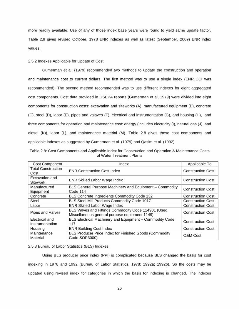
26

more readily available. Use of any of those index base years were found to yield same update factor.

Table 2.9 gives revised October, 1978 ENR indexes as well as latest (September, 2009) ENR index

values.

2.5.2 Indexes Applicable for Update of Cost

Gumerman et al. (1979) recommended two methods to update the construction and operation

and maintenance cost to current dollars. The first method was to use a single index (ENR CCI was

recommended). The second method recommended was to use different indexes for eight aggregated

cost components. Cost data provided in USEPA reports (Gumerman et al, 1979) were divided into eight

components for construction costs: excavation and siteworks (A), manufactured equipment (B), concrete

(C), steel (D), labor (E), pipes and valaves (F), electrical and instrumentation (G), and housing (H), and

three components for operation and maintenance cost: energy (includes electricity (I), natural gas (J), and

diesel (K)), labor (L), and maintenance material (M). Table 2.8 gives these cost components and

applicable indexes as suggested by Gumerman et al. (1979) and Qasim et al. (1992).

Table 2.8: Cost Components and Applicable Index for Construction and Operation & Maintenance Costs of Water Treatment Plants

Cost Component Index Applicable To Total Construction Cost

ENR Construction Cost Index Construction Cost

Excavation and Sitework

ENR Skilled Labor Wage Index Construction Cost

Manufactured Equipment

BLS General Purpose Machinery and Equipment – Commodity Code 114

Construction Cost

Concrete BLS Concrete Ingredients Commodity Code 132 Construction Cost Steel BLS Steel Mill Products Commodity Code 1017 Construction Cost Labor ENR Skilled Labor Wage Index Construction Cost

Pipes and Valves BLS Valves and Fittings Commodity Code 114901 (Used Miscellaneous general purpose equipment 1149)

Construction Cost

Electrical and Instrumentation

BLS Electrical Machinery and Equipment – Commodity Code 117

Construction Cost

Housing ENR Building Cost Index Construction Cost Maintenance Material

BLS Producer Price Index for Finished Goods (Commodity Code SOP3000)

O&M Cost

2.5.3 Bureau of Labor Statistics (BLS) Indexes

Using BLS producer price index (PPI) is complicated because BLS changed the basis for cost

indexing in 1978 and 1992 (Bureau of Labor Statistics, 1978; 1992a; 1992b). So the costs may be

updated using revised index for categories in which the basis for indexing is changed. The indexes

27

provided in the USEPA report provides BLS indexes with 1967 as base year. Modified 1978 October

indexes can also be obtained from official BLS website (Bureau of Labor Statistics, 2009). Table 2.9 gives

October, 1978 modified BLS index values as well September, 2009 index values.

Table 2.9: October 1978, Modified October 1978 and September 2009 Index Values

Index October 1978 Value of Index

Modified October 1978 Value of Index

Updated September 2009 Value of Index

ENR Construction Cost Index 265.38 (1967 = 100)

2859.0 (1913 = 100)

8585.71 (1913 = 100)

ENR Skilled Labor Wage Index 247.0 (1967 = 100)

2467.8 (1913 = 100)

8251.14 (1913 = 100)

BLS General Purpose Machinery and Equipment – Commodity Code 114

221.3 (1967 = 100)

72.9 (1982 = 100)

199.1* (1982 = 100)

BLS Concrete Ingredients Commodity Code 132 221.1 (1967 = 100)

71.6 (1982 = 100)

235.2* (1982 = 100)

BLS Steel Mill Products Commodity Code 1017 262.1 (1967 = 100)

75.0 (1982 = 100)

169.2* (1982 = 100)

BLS Valves and Fittings Commodity Code 114901 (Used Miscellaneous general purpose equipment 1149)

236.4 (1967 = 100)

70.2 (1982 = 100)

227.4* (1982 = 100)

BLS Electrical Machinery and Equipment – Commodity Code 117

167.5 (1967 = 100)

72.3 (1982 = 100)

113.7* (1982 = 100)

ENR Building Cost Index 254.8 (1967 = 100)

1727.5 (1913 = 100)

4764.44 (1913 = 100)

BLS Producer Price Index for Finished Goods (Commodity Code SOP3000)

199.7 (1967 = 100)

71.6 (1982 = 100)

173.4* (1982 = 100)

Adapted from Gumerman et al.(1979); Bureau of Labor Statistics (2009); Engineering News-Record

(1978 & 2009)

2.6 Present worth and annual equivalent worth calculation

Present worth (PW) of annual operation and maintenance cost is a minimum sum that must be

invested today at a given interest rate to pay for O&M cost every year throughout the life of the water

treatment plant. Equivalent annual cost is uniform series of expenditures at the end of each year that is

equivalent to different nonuniform capital and O&M expenditures made during the life cycle of the

treatment plant (Qasim et al., 1992). Equivalent annual cost is used to calculate cost per unit of water

treated. Also, when different alternatives are considered, equivalent annual costs are used to compare

and select the most cost effective alternative.

The present worth of annual O&M cost, and equivalent annual costs are obtained from

Equations 2.4, and 2.5 respectively.

28

PW of annual O&M cost = (total annual O&M cost) x CRF–1 ........................................ (2.4)

Equivalent annual cost, $/year = project PW x CRF ..................................................... (2.5)

Where,

PW = present worth

CRF = capital recovery factor = i/(1 – (1 + i)–n)

i = interest rate

n = design period, years;

2.7 Chapter Summary

Various treatment units combine to form a process train in a water treatment plant. Water quality

is the first indicator of types of unit operations and processes required in a treatment plant. Within these

unit operations and processes, there are different alternatives that can be used for same purpose. For

example, if clarifier is considered, designer has options of rectangular, circular, or upflow clarifiers.

Therefore, it is important to know, firstly, what treatment processes are required (for example if a clarifier

is required in this case), and secondly which is alternative is most cost effective. Various unit operations

and processes were discussed in this chapter.

Historical cost data for treatment units are available in literatures. The method to update these

costs primarily utilizes cost indexes like ENR and BLS indexes. Regression analysis is a tool to come up

with equations from set of data. The project feasibility and alternative evaluations are carried out by

calculating present worth, and annual equivalent worth of project alternatives. The information consisted

in this chapter are necessarily findings of the literature search and does not contain any opinion of the

author of this thesis.

29

CHAPTER 3

METHODOLOGY

3.1 Introduction

This chapter discusses the methodology adopted to obtain the final results of this research. The

overview of the methodology was listed in Chapter 1. This chapter provides details of methodology of this

research.

3.2 Comparison of Cost Update Methods

One of the objectives of this research was to make it possible for future updates of construction

and O&M cost data using single index. Use of single index is simple. However, use of multiple indexes

provides more accurate data. It was necessary to observe how the results obtained by using single and

multiple indexes vary with time involved in cost update. For this purpose, five treatment units: (i) chlorine

storage and feed system (2000 lb/day capacity), (ii) liquid alum feed system (540 lb/hr capacity), (iii)

rectangular clarifier (3600 ft2 surface area), (iv) gravity filtration structure (50 mgd capacity), and (v) air-

water backwash (1400 ft2 filter area capacity). Construction costs of each of these treatment units were

updated for every year from 1978 to 2009 by following three methods:

3.2.1 Single Index

ENR Construction Cost Index (CCI) was used to update 1978 October construction cost. Average

yearly index values were used to update the construction cost to each year from 1978 to 2009.

3.2.2 Multiple Indexes

Cost indexes listed in Table 2.8 were used to applicable construction cost components. Average

yearly index values were used to update the construction cost to each year from 1978 to 2009.

3.2.3Controlled Single Index

Updating by controlled single index value involved using both single and multiple indexes. This

approach was adopted to see if difference in results from using single and multiple indexes could be

30

controlled. The procedure adopted for this approach is as follows: (a) Single ENR CCI was used to

update construction cost for each year from 1978 to 1983. (b) Multiple indexes were used for construction

cost update to year 1984. (c) 1984 construction cost obtained from step (b) was used with single ENR

CCI to update construction cost for each year from 1985 to 1989. (d) Similarly, multiple indexes were

used for construction cost update to years 1990, 1996, 2002, and 2008. (e) 1990, 1996, 2002, and 2008

construction costs were respectively updated by using single ENR CCI to 1991-1995, 1997-2001, 2003-

2007 and 2009 construction costs.

3.3 Update of Construction and O&M Cost Data

Gumerman et al. (1979) provided October 1978 construction and O&M cost data for different

treatment units applicable to water treatment plants of 1 mgd to 200 mgd (Volume 2) and 2500 gpd to 1

mgd (Volume 3). It was necessary for these cost data to be updated to 2009 cost data. This update would

allow further updates to be done by using single index. For this purpose, each of October 1978

construction and O&M cost data were updated to September 2009 costs.

Construction costs were updated by using multiple cost indexes for different construction cost

components as listed in Table 2.8. The index values listed in Table 2.9 were used. Installed membrane

equipment costs were updated to September, 2009 costs by using BLS General Purpose Machinery and

Equipment – Commodity Code 114.

The O&M costs include cost for energy (electricity, natural gas, and diesel), labor, and

maintenance materials. The estimates provided by Gumerman et al. (1979) are based on unit energy cost

of $0.03/kW.h of electricity, $0.0013/scf of natural gas, and $0.45/gal of diesel. Unit labor costs are based

on $10/ labor-hr. October, 1978 O&M costs data were updated to September, 2009 O&M cost data. The

energy cost update was based on unit energy cost of $0.0981/kW.h of electricity (Energy Information

Administration, 2010a), $0.00898/scf of natural gas (Energy Information Administration, 2010b) and

$2.626/gal of diesel (Energy Information Administration, 2010c). Likewise, labor cost update was based

on $ 45.82/ labor-hr (Engineering News Records, 2009). October, 1978 maintenance material costs were

updated to September, 2009 maintenance material costs by using BLS Producer Price Index (PPI) for

Finished Goods (Commodity Code SOP3000).

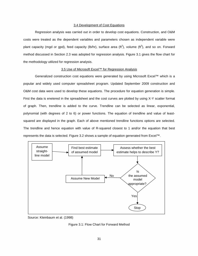
31

3.4 Development of Cost Equations

Regression analysis was carried out in order to develop cost equations. Construction, and O&M

costs were treated as the dependent variables and parameters chosen as independent variable were

plant capacity (mgd or gpd), feed capacity (lb/hr), surface area (ft2), volume (ft3), and so on. Forward

method discussed in Section 2.3 was adopted for regression analysis. Figure 3.1 gives the flow chart for

the methodology utilized for regression analysis.

3.5 Use of Microsoft Excel™ for Regression Analysis

Generalized construction cost equations were generated by using Microsoft Excel™ which is a

popular and widely used computer spreadsheet program. Updated September 2009 construction and

O&M cost data were used to develop these equations. The procedure for equation generation is simple.

First the data is enetered in the spreadsheet and the cost curves are plotted by using X-Y scatter format

of graph. Then, trendline is added to the curve. Trendline can be selected as linear, exponential,

polynomial (with degrees of 2 to 6) or power functions. The equation of trendline and value of least-

squared are displayed in the graph. Each of above mentioned trendline functions options are selected.

The trendline and hence equation with value of R-squared closest to 1 and/or the equation that best

represents the data is selected. Figure 3.2 shows a sample of equation generated from Excel™.

Source: Kleinbaum et al. (1998)

Figure 3.1: Flow Chart for Forward Method

Is

No the assumed model

appropriate?

Yes

Stop

Assume straight-

line model

Find best estimate of assumed model

Assess whether the best estimate helps to describe Y?

Assume New Model

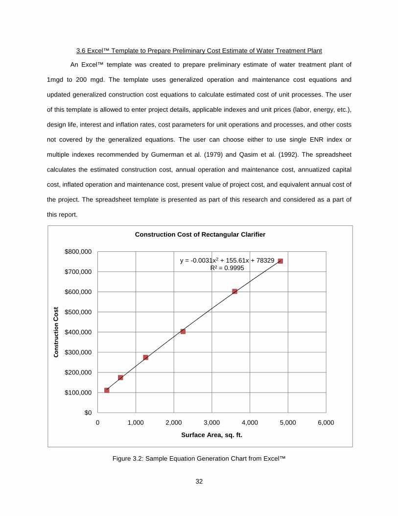
32

3.6 Excel™ Template to Prepare Preliminary Cost Estimate of Water Treatment Plant

An Excel™ template was created to prepare preliminary estimate of water treatment plant of

1mgd to 200 mgd. The template uses generalized operation and maintenance cost equations and

updated generalized construction cost equations to calculate estimated cost of unit processes. The user

of this template is allowed to enter project details, applicable indexes and unit prices (labor, energy, etc.),

design life, interest and inflation rates, cost parameters for unit operations and processes, and other costs

not covered by the generalized equations. The user can choose either to use single ENR index or

multiple indexes recommended by Gumerman et al. (1979) and Qasim et al. (1992). The spreadsheet

calculates the estimated construction cost, annual operation and maintenance cost, annuatized capital

cost, inflated operation and maintenance cost, present value of project cost, and equivalent annual cost of

the project. The spreadsheet template is presented as part of this research and considered as a part of

this report.

Figure 3.2: Sample Equation Generation Chart from Excel™

y = -0.0031x2 + 155.61x + 78329R² = 0.9995

$0

$100,000

$200,000

$300,000

$400,000

$500,000

$600,000

$700,000

$800,000

0 1,000 2,000 3,000 4,000 5,000 6,000

Co

nstru

ctio

n C

ost

Surface Area, sq. ft.

Construction Cost of Rectangular Clarifier

33

3.7 Chapter Summary

Firstly, difference in results by updating cost by single and multiple indexes were compared. A

new concept of controlled single index updating was introduced. From the result of this comparison, it

was decided to update all available historical data to September 2009 cost. This would enable further

updates to costs be done more accurately by using single cost index. Regression analysis was utilized to

generate cost equations which would yield September 2009 construction and O&M costs. Microsoft

Excel™ was used to carry out these regression analyses. The equations thus obtained were used to

devise an Excel™ template to estimate construction and O&M costs for water treatment plants.

34

CHAPTER 4

RESEARCH RESULTS

4.1 Introduction

This chapter presents the results of this research. The results of yearly cost updates made to five

treatment units listed in Section 3.2 are presented. Generalized construction and O&M cost equations are

presented in separate tables for 1 to 200 mgd water treatment plants and 2500 gpd to 1 mgd treatment

plants. An example to illustration calculation of construction cost, O&M cost, present worth, and

equivalent annual worth is presented. An Excel™ template for preliminary cost estimate of 1 mgd to 200

mgd water treatment plants is a result of this research. Features of this template are described in this

chapter. The template itself is a supplemental submission to this thesis.

4.2 Comparison of Cost Update Methods

Comparisons were made for results obtained from construction cost updates made by three

methods: (i) single index, (ii) multiple indexes, and (iii) controlled single index. These three methods are

explained in Section 3.2. The costs were updated for five treatment units: (i) chlorine storage and feed

system (2000 lb/day capacity), (ii) liquid alum feed system (540 lb/hr capacity), (iii) rectangular clarifier

(3600 ft2 surface area), (iv) gravity filtration structure (50 mgd capacity), and (v) air-water backwash (1400

ft2 filter area capacity). The results are presented in Figures 4.1, 4.2, 4.3, 4.4 and 4.5.

The results show that updated construction costs obtained from controlled single index method is

close to that obtained from multiple indexes. Controlled single index in the results shown were done at

interval of five years. Interval of eight and ten years were also tested which are shown in Appendix B.

4.3 Generalized Construction Cost Equations

Two sets of generalized construction cost equations were generated: (i) generalized construction

cost equations applicable for 1 mgd to 200 mgd water treatment plants (Table 4.1), and (ii) generalized

construction cost equations applicable for 2,500 gpd to 1 mgd water treatment plants (Table 4.2). These

cost equations yield the estimated construction cost for September, 2009. September, 2009 was selected

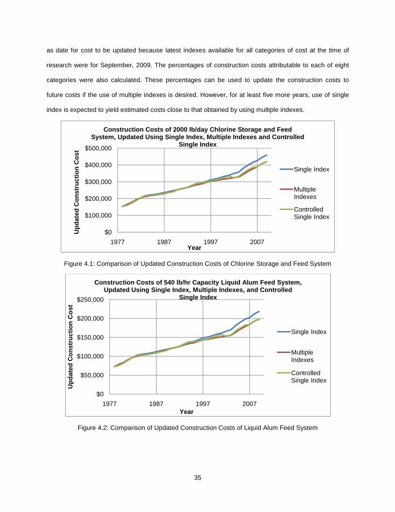
35

as date for cost to be updated because latest indexes available for all categories of cost at the time of

research were for September, 2009. The percentages of construction costs attributable to each of eight

categories were also calculated. These percentages can be used to update the construction costs to

future costs if the use of multiple indexes is desired. However, for at least five more years, use of single

index is expected to yield estimated costs close to that obtained by using multiple indexes.

Figure 4.1: Comparison of Updated Construction Costs of Chlorine Storage and Feed System

Figure 4.2: Comparison of Updated Construction Costs of Liquid Alum Feed System

$0

$100,000

$200,000

$300,000

$400,000

$500,000

1977 1987 1997 2007

Up

dat

ed C

on

stru

ctio

n C

ost

Year

Construction Costs of 2000 lb/day Chlorine Storage and Feed System, Updated Using Single Index, Multiple Indexes and Controlled

Single Index

Single Index

Multiple Indexes

Controlled Single Index

$0

$50,000

$100,000

$150,000

$200,000

$250,000

1977 1987 1997 2007

Up

dat

ed C

on

stru

ctio

n C

ost

Year

Construction Costs of 540 lb/hr Capacity Liquid Alum Feed System, Updated Using Single Index, Multiple Indexes, and Controlled

Single Index

Single Index

Multiple Indexes


36

Figure 4.3: Comparison of Updated Construction Costs of Rectangular Clarifier

Figure 4.4: Comparison of Updated Construction Costs of Gravity Filtration Structures

$0

$100,000

$200,000

$300,000

$400,000

$500,000

$600,000

$700,000

1977 1987 1997 2007

Up

dat

ed C

on

stru

ctio

n C

ost

Year

Construction Costs of 3600 ft2 Rectangular Clarifier, Updated Using Single Index, Multiple Indexes, and Controlled Single Index

Single Index

Multiple Indexes


$0

$1,000,000

$2,000,000

$3,000,000

$4,000,000

$5,000,000

$6,000,000

$7,000,000

1977 1987 1997 2007

Up

dat

ed C

on

stru

ctio

n C

ost

Year

Construction Costs of 50 mgd Gravity Filtration Structure, Updated Using Single Index, Multiple Indexes, and Controlled Single Index

Single Index

Multiple Indexes


37

Figure 4.5: Comparison of Updated Construction Costs of Gravity Filtration Structures

4.3.1 Generalized Operation and Maintenance Cost Equations

Two sets of generalized operation and maintenance cost equations were generated: (i)

generalized operation and maintenance cost equations applicable for 1 mgd to 200 mgd water treatment

plants (Table 4.3), and (ii) generalized operation and maintenance cost equations applicable for 2,500

gpd to 1 mgd water treatment plants (Table 4.4). These cost equations yield the estimated operation and

maintenance cost for September, 2009. The percentage of cost attributable to five categories, (i) energy,

(ii) natural gas, (iii) maintenance materials, (iv) labor, and (v) diesel, were also calculated.

$0

$100,000

$200,000

$300,000

$400,000

$500,000

$600,000

1977 1987 1997 2007

Up

dat

ed C

on

stru

ctio

n C

ost

Year

Construction Costs of 1400 ft2 Filter Area Capacity Air-Water Backwash, Updated Using Single Index, Multiple Indexes, and


Single Index

Multiple Indexes

38

Table 4.1: Generalized Construction Cost Equations Applicable for 1 to 200 mgd Water Treatment Plants

Treatment Units

Construction Costs

Cost Equations Eq.

No.

Component Cost-Percentages Applicable Ranges

of x

A B C D E F G H Minimu

m Maximu

m Raw Water Pumping Raw Water Pumping Facilities TDH = 30 ft. CC = 9355.4 x + 60290 4.1 40 19 36 5 1 200 TDH = 100 ft. CC = 12627 x + 68364 4.2 45 15 27 13 1 200 x = plant capacity, mgd Pretreatment Chlorine Storage and Feed Cylinder Storage CC = 3E–6 x3 – 0.0423 x2 + 267.97 x +

29368 4.3 40 6 4 3 47 10 10,000

On-site storage tank with rail delivery

CC = 1E–6 x3 – 0.0158 x2 + 98.896 x + 10708

4.4 80 2 10 4 3 1 2,000 10,000

Direct feed from rail car CC = 0.0019 x2 + 13.734 x + 47956 4.5 82 8 5 3 2 2,000 10,000 x = chlorine feed capacity, lb/day Chlorine Dioxide Generating and Feed

CC = – 0.0783 x2 + 663.68 x + 82909 4.6 29 36 3 2 30 1 5,000

x = chlorine dioxide feed capacity, lb/day Ozone Generations Systems CC = 0.0002 x3 – 1.3451 x2 + 4147.8 x +

212878 4.7 83 15 2 10 3,500

x = ozone generation capacity, lb/day Ozone Contact Chambers CC = 6E–6 x2 + 5.181 x + 41901 4.8 6 21 24 49 460 92,000 x = contact chamber volume, ft3 On-Site Hypochlorite Generation Systems

CC = 8E–6 x3 – 0.1413 x2 + 884.72 x + 87471

4.9 66 25 3 6 10 10,000

x = hypochlorite generation rate, lb/day Powdered Activated Carbon Feed Systems

CC = – 0.0577 x2 + 778.86 x + 175653 4.10 1 56 4 5 8 14 10 2 3.5 7,000

x = feed capacity, lb/hr Powdered Carbon Regeneration – Fluidized Bed Process

CC = 7E–7 x3 – 0.0361 x2 + 832.64 x + 2000000

4.11 49 42 8 1 209 33,360

x = regeneration capacity, lb/day

39


Treatment Units

Construction Costs

Cost Equations Eq.

No.


of x


m Maximu

m Powdered Carbon Regeneration – Atomized Suspension Process

CC = 511.53 x + 342140 4.12 85 7 8 1,000 10,000

x = regeneration capacity, lb/day Aeration Diffused Aeration Basin CC = 0.2287 x3 – 133.51 x2 + 64933 x +

287711 4.13 1 63 2 2 21 9 2 1.9 380

x = aeration basin volume, 1000 ft3 Aeration Towers CC = – 19.857 x2 + 25002 x + 175725 4.14 64 7 7 20 2 0.68 256 x = aeration tower volume, 1000 ft3 Coagulation, Precipitation and Flocculation Liquid Alum Feed System CC = – 0.0249 x2 + 280.21 x + 54288 4.15 64 14 2 4 16 5.4 5,400 Dry Alum Feed System CC = 240.78 x + 71071 4.16 41 4 5 3 47 10 5,000 x = feed capacity, lb/hr Ferrous Sulfate Feed Systems CC = – 0.002 x2 + 222.15 x + 63563 4.17 41 4 5 3 47 10.7 5,350 x = feed capacity, lb/hr Ferric Sulfate Feed Systems CC = – 0.001 x2 + 177.92 x + 63605 4.18 41 4 5 3 47 13.3 6,600 x = feed capacity, lb/hr Polymer Feed Systems CC = – 0.0055 x3 + 1.8481 x2 – 19.72 x +

54155 4.19 70 4 2 4 20 1 200

x = feed capacity, lb/day Sulfuric Acid Feed Systems CC = – 0.0029 x2 + 48.434 x + 22648 4.20 33 7 3 6 51 10 5,000 x = feed capacity, gpd Sodium Hydroxide Feed Systems

CC = 20.35 x + 36294 4.21 59 20 8 6 7 10 10,000

x = feed capacity, lb/day Rapid Mix, G = 300 /s CC = 0.0002 x2 + 22.776 x + 28584 4.22 4 38 10 10 23 15 100 20,000 x = total basin volume, ft3 Rapid Mix, G = 600 /s CC = 0.0002 x2 + 29.209 x + 30388 4.23 3 47 8 8 21 13 100 20,000 x = total basin volume, ft3 Rapid Mix, G = 900 /s CC = 0.0002 x2 + 55.443 x + 29756 4.24 2 68 5 5 16 4 100 20,000 x = total basin volume, ft3

40


Treatment Units

Construction Costs

Cost Equations Eq.

No.


of x


m Maximu

m Flocculation Horizontal Paddle Systems, G = 20 /s

CC = 5E–12 x3 – 7E–6 x2 + 6.8748 x + 162853

4.25 6 17 18 18 30 11 1,800 1,000,000

Horizontal Paddle Systems, G = 50 /s

CC = 5E–12 x3 – 7E–06 x2 + 7.7415 x + 158139

4.26 5 25 15 15 30 10 1,800 1,000,000

Horizontal Paddle Systems, G = 80 /s

CC = – 0.000004 x2 + 9.3239 x + 160468 4.27 4 35 11 12 30 8 1,800 500,000

Vertical Turbine Flocculators, G = 20 /s

CC = – 0.0005 x2 + 26.863 x + 34588 4.28 3 22 11 13 35 16 1,800 25,000


CC = – 0.0005 x2 + 28.042 x + 32609 4.29 3 22 11 13 35 16 1,800 25,000


CC = – 0.0005 x2 + 27.306 x + 33732 4.30 3 24 11 12 35 15 1,800 25,000

x = total basin volume, ft3 Sedimentation Upflow Solids Contact Clarifiers CC = 3E–7 x3 – 0.0095 x2 + 167.45 x +

181434 4.31 5 49 9 8 28 1 255 14,544

x = net effective settling area, ft2 Circular Clarifiers CC = – 0.0005 x2 + 86.89 x + 182801 4.32 3 31 9 33 16 6 2 707 31,416 Rectangular Clarifiers CC = – 0.0031 x2 + 155.61 x + 78329 4.33 4 26 11 22 24 12 1 240 4,800 x = surface area, ft2 Tube Settling Modules CC = – 5.6888 x2 + 17121 x + 21973 4.34 51 25 24 1 200 x = tube module area, ft2 Contact Basins CC = 611.54 x0.5804 4.35 8 22 26 44 2,640 52,800 x = basin volume, ft2 Filtration Gravity Filtration Structures CC = 2.642 x3 – 822.49 x2 + 138705 x +

453613 4.36 1 18 7 3 24 26 3 18 1 200

x = plant flow rate, mgd Filtration Media Rapid Sand CC = 7558.4 x + 13488

4.37 100

1 200

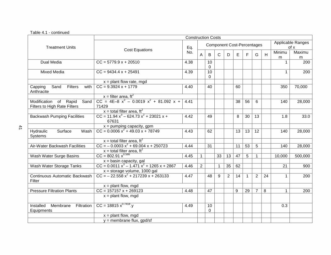
41


Treatment Units

Construction Costs

Cost Equations Eq.

No.


of x


m Maximu

m Dual Media CC = 5779.9 x + 20510 4.38 10

0 1 200

Mixed Media CC = 9434.4 x + 25491 4.39 100

1 200

x = plant flow rate, mgd Capping Sand Filters with Anthracite

CC = 9.3924 x + 1779 4.40 40 60 350 70,000

x = filter area, ft2 Modification of Rapid Sand Filters to High Rate Filters

CC = 4E–8 x3 – 0.0019 x2 + 81.092 x + 71429

4.41 38 56 6 140 28,000

x = total filter area, ft2 Backwash Pumping Facilities CC = 11.94 x3 – 624.73 x2 + 23021 x +

67631 4.42 49 8 30 13 1.8 33.0

x = pumping capacity, gpm Hydraulic Surface Wash Systems

CC = 0.0006 x2 + 49.03 x + 78749 4.43 62 13 13 12 140 28,000

x = total filter area, ft2 Air-Water Backwash Facilities CC = – 0.0003 x2 + 69.004 x + 250723 4.44 31 11 53 5 140 28,000 x = total filter area, ft2 Wash Water Surge Basins CC = 802.91 x0.586 4.45 1 33 13 47 5 1 10,000 500,000 x = basin capacity, gal Wash Water Storage Tanks CC = 0.0011 x3 – 1.471 x2 + 1265 x + 2867 4.46 2 1 35 62 21 900 x = storage volume, 1000 gal Continuous Automatic Backwash Filter

CC = – 22.558 x2 + 217239 x + 263133 4.47 48 9 2 14 1 2 24 1 200

x = plant flow, mgd Pressure Filtration Plants CC = 157157 x + 269123 4.48 47 9 29 7 8 1 200 x = plant flow, mgd

Installed Membrane Filtration Equipments

CC = 18815 x0.7418.y 4.49 100

0.3

x = plant flow, mgd y = membrane flux, gpd/sf

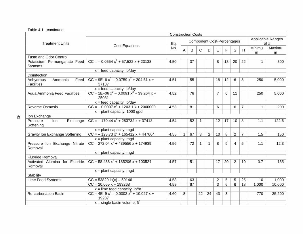
42


Treatment Units

Construction Costs

Cost Equations Eq.

No.


of x


m Maximu

m Taste and Odor Control Potassium Permanganate Feed Systems

CC = – 0.0554 x2 + 57.522 x + 23138 4.50 37 8 13 20 22 1 500

x = feed capacity, lb/day Disinfection Anhydrous Ammonia Feed Facilities

CC = 9E–6 x3 – 0.0759 x2 + 204.51 x + 37137

4.51 55 18 12 6 8 250 5,000

x = feed capacity, lb/day Aqua Ammonia Feed Facilities CC = 1E–06 x3 – 0.0091 x2 + 39.264 x +

25081 4.52 76 7 6 11 250 5,000

x = feed capacity, lb/day Reverse Osmosis CC = – 0.0007 x2 + 1203.1 x + 2000000 4.53 81 6 6 7 1 200 x = plant capacity, 1000 gpd Ion Exchange Pressure Ion Exchange Softening

CC = – 170.44 x2 + 283732 x + 37413 4.54 52 1 12 17 10 8 1.1 122.6

x = plant capacity, mgd Gravity Ion Exchange Softening CC = – 123.73 x2 + 165412 x + 447664 4.55 1 67 3 2 10 8 2 7 1.5 150 x = plant capacity, mgd Pressure Ion Exchange Nitrate Removal

CC = 272.04 x2 + 439556 x + 174939 4.56 72 1 1 8 9 4 5 1.1 12.3

x = plant capacity, mgd Fluoride Removal Activated Alumina for Fluoride Removal

CC = 58.438 x2 + 185206 x + 103524 4.57 51 17 20 2 10 0.7 135

x = plant capacity, mgd Stability Lime Feed Systems CC = 53829 ln(x) – 59146 4.58 63 2 5 5 25 10 1,000

CC = 20.065 x + 193268 4.59 67 3 6 6 18 1,000 10,000 x = lime feed capacity, lb/hr Re-carbonation Basin CC = 4E–9 x3 – 0.0002 x2 + 10.027 x +

19287 4.60 8 22 24 43 3 770 35,200

x = single basin volume, ft3

43


Treatment Units

Construction Costs

Cost Equations Eq.

No.


of x


m Maximu

m Re-carbonation – Liquid CO2 as CO2 Source

CC = 9E–8 x3 – 0.001 x2 + 42.578 x + 130812

4.61 55 25 13 7 380 15,000

x = installed capacity, lb/day Re-carbonation – Submerged Burners as CO2 Source

CC = – 7E–11 x4 + 2E–6 x3 – 0.0107 x2 + 46.074 x + 128953

4.62 55 24 17 4 500 10,000

x = installed capacity, lb/day Re-carbonation – Stack Gas as CO2 Source

CC = 1490.2 x0.5399 4.63 46 31 15 8 2,500 50,000

x = installed capacity, lb/CO2/day Multiple Hearth Recalcination CC = 0.0005 x3 – 2.9835 x2 + 7188.6 x +

1000000 4.64 60 31 1 8 179 2,925

x = effective hearth area, ft2 Concrete Gravity Carbon Contactors, 7.5 min Empty Bed Contact Time and 5 ft Bed Depth

CC = 1E–06 x3 – 0.0452 x2 + 1094.8 x + 502902

4.65 1 18 6 3 20 33 3 16 140 28,000

x = total contactor area, ft2 Concrete Gravity Carbon Contactors, 12.5 min Empty Bed Contact Time and 8.3 ft Bed Depth

CC = 1E-06 x3 – 0.0492 x2 + 1171.5 x + 561247

4.66 1 17 7 3 24 30 3 15 140 28,000

x = total contactor area, ft2 Steel Gravity Carbon Contactors, 20 ft Diameter, 20 ft deep Tanks

CC = – 429.69 x2 + 491322 x + 8537 4.67 43 1 10 22 3 21 5 100

x = number of contactors

Steel Gravity Carbon Contactors, 30 ft Diameter, 20 ft deep Tanks

CC = 897917 x + 822066 4.68 44 1 10 22 3 20 10 40

x = number of contactors Pressure Carbon Contactors – 7.5 min Empty Bed Contact Time and 5 ft Bed Depth

CC = 1778.5 x + 136180 4.69 50 1 9 20 6 14 157 6,786

x = total contactor area, ft2

44


Treatment Units

Construction Costs

Cost Equations Eq.

No.


of x


m Maximu

m Pressure Carbon Contactors – 15 min Empty Bed Contact Time and 10 ft Bed Depth

CC = 2000.7 x + 154612 4.70 49 1 8 19 6 17 157 6,786

x = total contactor area, ft2 Pressure Carbon Contactors – 30 min Empty Bed Contact Time and 20 ft Bed Depth

CC = 3185.1 x + 205007 4.71 51 6 19 4 20 157 6,786

x = total contactor area, ft2 Conversion of Sand Filter to Carbon Contactor (Carbon Bed Depth = 30”)

CC = – 0.00004 x2 + 60.712 x + 69940 4.72 10 26 63 1 875 175,000

x = contactor volume, ft3 Off-Site Regional Carbon Regeneration – Handling and Transportation

CC = 0.0004 x2 + 41.116 x + 40083 4.73 15 3 30 47 5 1,000 20,000

x = on-site storage capacity, ft3 Multiple Hearth Granular Carbon Regeneration

CC = 406413 x0.4067 4.74 50 33 2 1 14 27 1,509

x = furnace hearth area, ft2 Infrared Carbon Regeneration Furnace

CC = 1E–8 x3 – 0.0011 x2 + 87.308 x + 601190

4.75 64 21 1 5 9 2,400 60,000

x = regeneration capacity, lb/day Granular Carbon Regeneration – Fluid Bed Process

CC = 2E–8 x3 – 0.0018 x2 + 93.965 x + 2000000

4.76 66 25 1 8 6,000 24,000

x = regeneration capacity, lb/day Clear Water Storage and Distribution Below-Ground Clearwell Storage CC = – 0.0697 x2+ 1161.9 x + 115431 4.77 3 43 19 34 1 10 7,500 x = clearwell capacity, 1000 gal Ground-Level Clearwell Storage CC = 4E–06 x3 – 0.0636 x2 + 585.7 x +

86980 4.78 76 10 5 2 6 1 8.5 9,400.4

x = clearwell capacity, 1000 gal

45


Treatment Units

Construction Costs

Cost Equations Eq.

No.


of x


m Maximu

m Finished Water Pumping Facilities

TDH = 30 ft. CC = – 4.8889 x2 + 13015 x + 44288 4.79 44 13 28 15 1.5 300 TDH = 100 ft. CC = 0.1909 x3 – 85.9 x2 + 28173 x + 53608 4.80 60 10 17 13 1.5 300 x = plant capacity, mgd In-Plant Pumping CC = 11.758 x2 + 12402 x + 84932 4.81 17 2 2 39 28 6 6 1 200 x = plant flow, mgd Residuals Processing and Disposal Pressure Diatomite Filters CC = – 76.954 x2 + 218790 x + 498789 4.82 61 18 6 9 6 1 200 x = plant flow, mgd Vacuum Diatomite Filters CC = 62.099 x2 + 280763 x + 207572 4.83 32 26 25 3 14 1 200 x = plant flow, mgd Chemical Sludge Pumping – Unthickened Sludge

CC = 1E–6 x3 – 0.0246 x2 + 174.33 x + 89824

4.84 2 15 6 4 31 30 5 7 20 10,000

x = pumping capacity, gpm Chemical Sludge Pumping – Thickened Sludge

CC = 0.0004 x3 – 0.7412 x2 + 494.82 x + 22130

4.85 68 16 4 3 9 5 1,250

x = pumping capacity, gpm Gravity Sludge Thickeners CC = 0.0039 x4 – 1.0079 x3 + 82.537 x2 +

2833.3 x + 68377 4.86 4 39 13 12 31 1 20 150

x = diameter, ft Vacuum Filters CC = – 0.1664 x2 + 1863 x + 465811 4.87 50 26 2 1 21 9.4 1,320 x = total filter area, ft2 Sludge Dewatering Lagoons CC = 16.041 x3 – 1483.3 x2 + 60825 x +

14155 4.88 5

4 4 26 16 0.3 60

x = effective storage volume, million gallons Filter Press CC = 0.0093 x3 – 12.453 x2 + 9607.7 x +

734176 4.89 61 21 1 1 16 4.3 896

x = total filter press volume, ft3 Decanter Centrifuges CC = 0.0133 x3 – 12.685 x2 + 5635.3 x +

411407 4.90 50 19 7 1 23 10 500

x = machine capacity, gpm

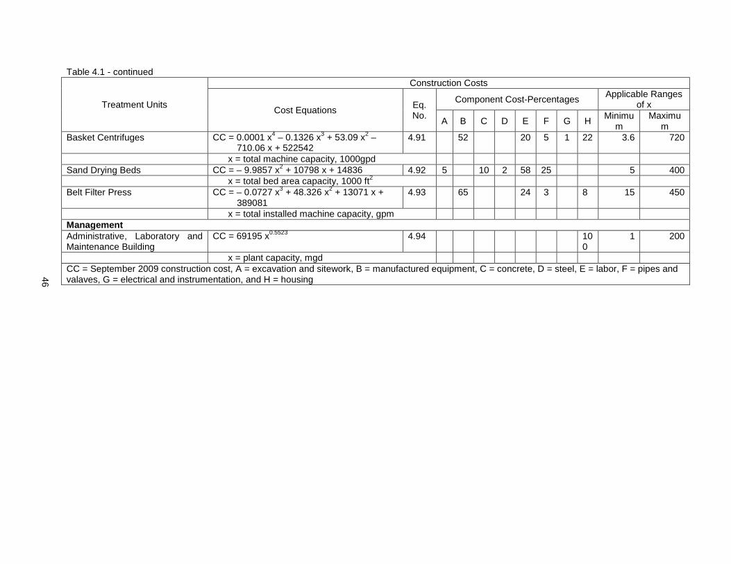
46


Treatment Units

Construction Costs

Cost Equations Eq.

No.


of x


m Maximu

m Basket Centrifuges CC = 0.0001 x4 – 0.1326 x3 + 53.09 x2 –

710.06 x + 522542 4.91 52 20 5 1 22 3.6 720

x = total machine capacity, 1000gpd Sand Drying Beds CC = – 9.9857 x2 + 10798 x + 14836 4.92 5 10 2 58 25 5 400 x = total bed area capacity, 1000 ft2 Belt Filter Press CC = – 0.0727 x3 + 48.326 x2 + 13071 x +

389081 4.93 65 24 3 8 15 450

x = total installed machine capacity, gpm Management Administrative, Laboratory and Maintenance Building

CC = 69195 x0.5523 4.94 100

1 200

x = plant capacity, mgd CC = September 2009 construction cost, A = excavation and sitework, B = manufactured equipment, C = concrete, D = steel, E = labor, F = pipes and valaves, G = electrical and instrumentation, and H = housing

47

Table 4.2: Generalized Construction Cost Equations Applicable for 2,500 gpd to 1 mgd Water Treatment Plants

Treatment Units

Construction Costs

Cost Equations Eq. No.


of x


m Maximu

m Package Complete Treatment Plants

CC = – 0.1356 x2 + 971.3 x + 151058 4.95 1 41 1 12 3 13 29

Filtration Rate 2 gpm/sq. ft. x = 2.5 x plant capacity, gpm 4 560 Filtration Rate 5 gpm/sq. ft. x = plant capacity, gpm 10 1,400 Package Gravity Filter Plants CC = 0.0004 x3 – 0.7213 x2 + 860.37 x +

268511 4.96 1 23 16 10 7 11 32

Filtration Rate 2 gpm/sq. ft. x = 2.5 x plant capacity, gpm 80 560 Filtration Rate 5 gpm/sq. ft. x = plant capacity, gpm 200 1,400 Package Pressure Filtration Plants

CC = 0.0059 x3 – 5.0895 x2 + 2024.7 x + 60520

4.97 41 2 16 2 7 32

Filtration Rate 2 gpm/sq. ft. x = 2.5 x plant capacity, gpm 80 560 Filtration Rate 5 gpm/sq. ft. x = plant capacity, gpm 200 1,400 Filter Media Rapid Sand CC = 0.0005 x3 – 0.2286 x2 + 104.37 x + 402 4.98 10

0 4 280

Dual Media (Coal-Sand) CC = – 0.0259 x2 + 121.91 x + 596 4.99 100

4 280

Mixed Media CC = 0.0021 x3 – 0.9505 x2 + 275.35 x + 2607

4.100 100

4 280

x = filter area, ft2 Package Pressure Diatomite Filters

CC = – 0.0003 x3 + 0.4823 x2 + 179.64 x + 127018

4.101 1 57 1 10 4 3 24 28 1,000

x = plant capacity, 1000 gpd Package Vacuum Diatomite Filters

CC = 0.0013 x3 – 1.4383 x2 + 887.4 x + 119909

4.102 1 67 1 5 6 1 19 30 720

x = plant flow, gpm Package Ultrafiltration Plants CC = 0.0003 x3 – 0.8109 x2 + 2016.9 x +

38246 4.103 63 1 9 1 8 18 2.5 1,000

x = plant flow, 1000 gpd

48


Treatment Units

Construction Costs



of x


m Maximu

m Package Granular Activated Carbon Columns

CC = 0.0084 x3 – 5.2233 x2 + 1318.4 x + 27144

4.104 24 2 24 13 2 35 1.7 350

x = plant flow, gpm Potassium Permanganate Feed Systems

CC = 20,323 4.105 21 6 6 2 65 1

x = plant capacity, mgd Polymer Feed Systems CC = 50,974 4.106 68 5 2 4 21 1 x = plant capacity, mgd Powdered Activated Carbon Feed Systems

CC = – 37.856 x2 + 888.08 x + 8061 4.107 81 13 6 1 10

x = feed system capacity, lb/hr Direct Feed Gas Chlorination CC = 11,838 4.108 34 10 3 3 50 100 x = feed capacity, lb/day Sodium Hypochlorite Solution Feed

CC = 11,954 4.109 29 10 9 3 49 2,5000 1,000,000

x = plant capacity, gpd Ozone Generation Systems CC = – 45.636 x2 + 7302.4x + 58785 4.110 65 13 22 0.5 10 x = ozone generation capacity, lb/day Ozone Contact Chambers CC = 5.7586 x0.9048 4.111 81 3 1 15 850 13,540 x = contactor volume, gal Chlorine Dioxide Generating and Feed System

CC = 26,683 4.112 48 8 7 3 34 50

x = chlorine generating capacity, lb/day Ultraviolet Light Disinfection CC = 0.0065 x2 + 93.179 x + 9042 4.113 1 58 5 4 4 4 24 10 780 x = plant capacity, gpm Reverse Osmosis CC = – 1E–6 x2 + 3.4414 x + 26179 4.114 59 13 12 16 2,500 1,000,00

0 x = plant capacity, gpd Pressure Ion Exchange Softening

CC = 2E–13 x3 – 4E–07 x2 + 0.4275 x + 132617

4.115 1 34 2 2 13 20 16 12 70,000 860,000

x = plant capacity, gpd

49


Treatment Units

Construction Costs



of x


m Maximu

m Pressure Ion Exchange Nitrate Removal

CC = 3E–13 x3 – 4E–7 x2 + 0.5706 x + 130264

4.116 49 1 1 9 17 13 10 70,000 830,000

x = plant capacity, gpd Activated Alumina Fluoride Removal

CC = 5600.1 x0.2911 4.117 24 15 27 23 11 12,700 910,000

x = plant capacity, gpd Bone Char Fluoride Removal CC = – 2E–18x4 + 4E–12x3 – 2E–6 x2 +

0.8756 x + 126895 4.118 31 17 19 15 18 16300 800,000

x = plant capacity, gpd Package Raw Water Pumping Facilities, TDH = 50 ft

CC = – 7E–7 x4 + 0.0012 x3 – 0.7024 x2 + 217.03 x + 29989

4.119 9 52 5 23 9 2 20 700

x = pumping capacity, gpm Package High Service Pumping Stations

CC = – 0.0189 x2 + 49.995 x + 28397 4.120 78 14 6 2 30 1,100

x = pumping capacity, gpm Steel Backwash/Clearwell Tanks CC = – 1E–5 x2 + 2.5112x + 3117 4.121 2 4 79 15 500 30,000 x = storage volume, gal Sludge Dewatering Lagoons CC = 6E–10 x3 – 0.00002 x2 + 0.6293 x +

5960 4.122 3

4 13 28 25 1,500 30,000

x = effective lagoon volume, ft3 Sand Drying Beds CC = – 0.004 x2 + 21.321 x + 2593 4.123 5 36 4 27 28 200 800 x = bed area, ft2 CC = September 2009 construction cost, A = excavation and sitework, B = manufactured equipment, C = concrete, D = steel, E = labor, F = pipes and valaves, G = electrical and instrumentation, and H = housing

50

Table 4.3: Generalized O&M Cost Equations Applicable to 1 mgd to 200 mgd Water Treatment Plants

Treatment Units

Operation and Maintenance Costs


Component Cost-Percentages

Applicable Ranges of x

I J K L M Minim

um Maxim

um Raw Water Pumping Raw Water Pumping Facilities TDH = 30 ft. O&MC = 5768.2 x + 23723 4.124 73 22 5 1 200 TDH = 100 ft. O&MC = 8709.5 x + 23723 4.125 81 15 4 1 200 x = plant capacity, mgd Pretreatment Chlorine Storage and Feed Cylinder Storage O&MC = 5E–7 x3 – 0.0085 x2 + 65.019 x + 20205 4.126 18 74 8 10 10,000 On-site storage tank with rail delivery O&MC = – 0.003 x2 + 5.8195 x + 43965 4.127 2 75 23 2,000 10,000 Direct feed from rail car O&MC = – 0.00006 x2 + 2.1722 x + 42499 4.128 3 68 29 2,000 10,000 x = chlorine feed capacity, lb/day Chlorine Dioxide Generating and Feed O&MC = – 0.0106 x2 + 105.82 x + 32441 4.129 6 85 9 1 5,000 x = chlorine dioxide feed capacity, lb/day Ozone Generations Systems O&MC = – 0.0093 x2 + 354.32 x + 33867 4.130 76 16 8 10 3,500 x = ozone generation capacity, lb/day On-Site Hypochlorite Generation Systems O&MC = – 0.0034 x2 + 147.44 x + 25004 4.131 70 20 10 10 10,000 x = hypochlorite generation rate, lb/day Powdered Activated Carbon Feed Systems O&MC = – 0.0204 x2 + 262.07 x + 54144 4.132 27 56 17 3.5 7,000 x = feed capacity, lb/hr Powdered Carbon Regeneration – Fluidized Bed Process

O&MC = 3E–8 x3 – 0.012 x2 + 300.16 x + 68295 4.133 41 44 13 2 220 32,570

x = regeneration capacity, lb/day Powdered Carbon Regeneration – Atomized Suspension Process

O&MC = 56.048 x + 53991 4.134 7 75 16 2 1,000 10,000

x = regeneration capacity, lb/day Aeration Diffused Aeration Basin O&MC = 19557 x + 76673 4.135 74 25 1 1.9 380 x = aeration basin volume, 1000 ft3 Aeration Towers O&MC = 1525.2 x + 4343 4.136 63 22 15 0.68 256 x = aeration tower volume, 1000 ft3

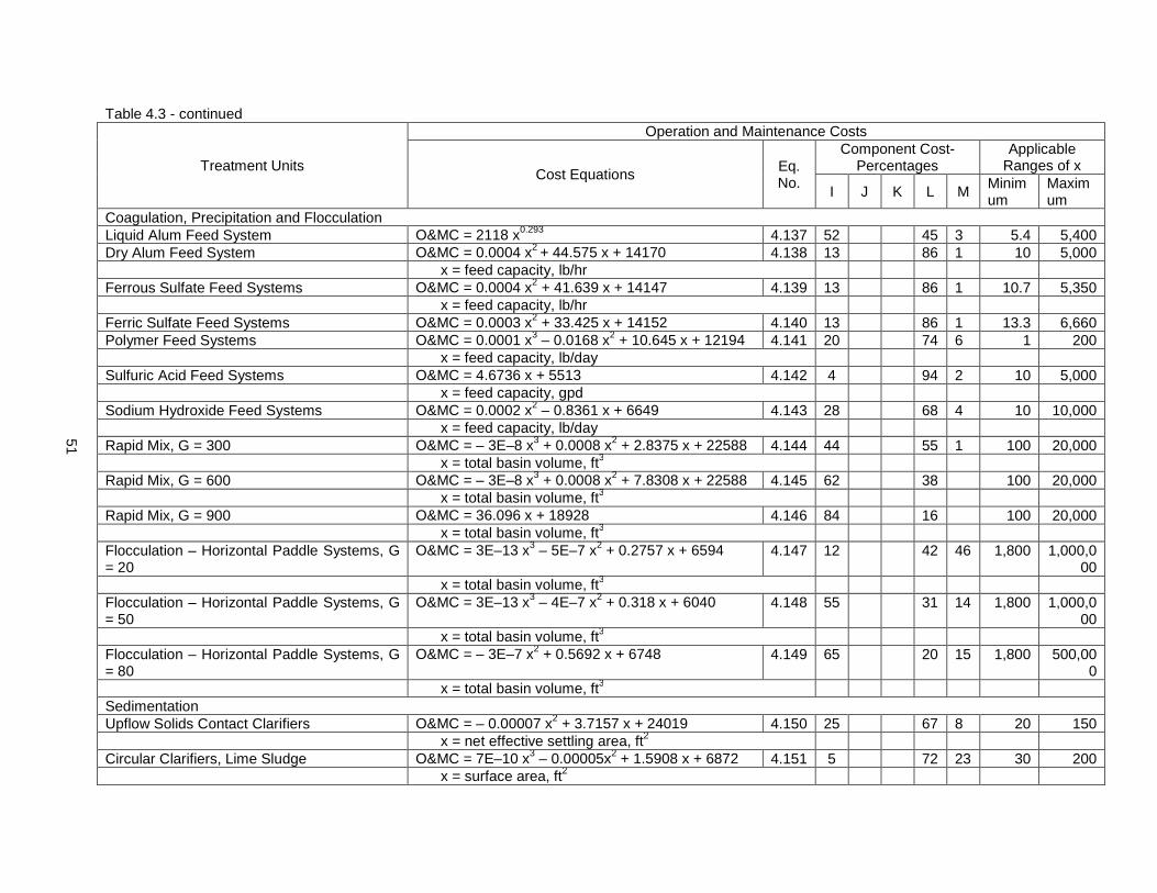
51


Treatment Units





I J K L M Minimum

Maximum

Coagulation, Precipitation and Flocculation Liquid Alum Feed System O&MC = 2118 x0.293 4.137 52 45 3 5.4 5,400 Dry Alum Feed System O&MC = 0.0004 x2 + 44.575 x + 14170 4.138 13 86 1 10 5,000 x = feed capacity, lb/hr Ferrous Sulfate Feed Systems O&MC = 0.0004 x2 + 41.639 x + 14147 4.139 13 86 1 10.7 5,350 x = feed capacity, lb/hr Ferric Sulfate Feed Systems O&MC = 0.0003 x2 + 33.425 x + 14152 4.140 13 86 1 13.3 6,660 Polymer Feed Systems O&MC = 0.0001 x3 – 0.0168 x2 + 10.645 x + 12194 4.141 20 74 6 1 200 x = feed capacity, lb/day Sulfuric Acid Feed Systems O&MC = 4.6736 x + 5513 4.142 4 94 2 10 5,000 x = feed capacity, gpd Sodium Hydroxide Feed Systems O&MC = 0.0002 x2 – 0.8361 x + 6649 4.143 28 68 4 10 10,000 x = feed capacity, lb/day Rapid Mix, G = 300 O&MC = – 3E–8 x3 + 0.0008 x2 + 2.8375 x + 22588 4.144 44 55 1 100 20,000 x = total basin volume, ft3 Rapid Mix, G = 600 O&MC = – 3E–8 x3 + 0.0008 x2 + 7.8308 x + 22588 4.145 62 38 100 20,000 x = total basin volume, ft3 Rapid Mix, G = 900 O&MC = 36.096 x + 18928 4.146 84 16 100 20,000 x = total basin volume, ft3 Flocculation – Horizontal Paddle Systems, G = 20

O&MC = 3E–13 x3 – 5E–7 x2 + 0.2757 x + 6594 4.147 12 42 46 1,800 1,000,000

x = total basin volume, ft3 Flocculation – Horizontal Paddle Systems, G = 50

O&MC = 3E–13 x3 – 4E–7 x2 + 0.318 x + 6040 4.148 55 31 14 1,800 1,000,000

x = total basin volume, ft3 Flocculation – Horizontal Paddle Systems, G = 80

O&MC = – 3E–7 x2 + 0.5692 x + 6748 4.149 65 20 15 1,800 500,000

x = total basin volume, ft3 Sedimentation Upflow Solids Contact Clarifiers O&MC = – 0.00007 x2 + 3.7157 x + 24019 4.150 25 67 8 20 150 x = net effective settling area, ft2 Circular Clarifiers, Lime Sludge O&MC = 7E–10 x3 – 0.00005x2 + 1.5908 x + 6872 4.151 5 72 23 30 200 x = surface area, ft2

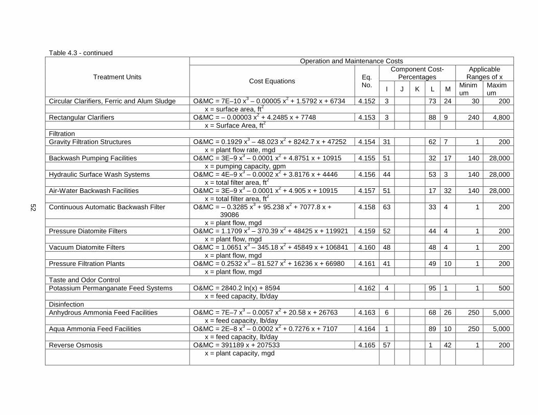
52


Treatment Units





I J K L M Minimum

Maximum

Circular Clarifiers, Ferric and Alum Sludge O&MC = 7E–10 x3 – 0.00005 x2 + 1.5792 x + 6734 4.152 3 73 24 30 200 x = surface area, ft2 Rectangular Clarifiers O&MC = – 0.00003 x2 + 4.2485 x + 7748 4.153 3 88 9 240 4,800 x = Surface Area, ft2 Filtration Gravity Filtration Structures O&MC = 0.1929 x3 – 48.023 x2 + 8242.7 x + 47252 4.154 31 62 7 1 200 x = plant flow rate, mgd Backwash Pumping Facilities O&MC = 3E–9 x3 – 0.0001 x2 + 4.8751 x + 10915 4.155 51 32 17 140 28,000 x = pumping capacity, gpm Hydraulic Surface Wash Systems O&MC = 4E–9 x3 – 0.0002 x2 + 3.8176 x + 4446 4.156 44 53 3 140 28,000 x = total filter area, ft2 Air-Water Backwash Facilities O&MC = 3E–9 x3 – 0.0001 x2 + 4.905 x + 10915 4.157 51 17 32 140 28,000 x = total filter area, ft2 Continuous Automatic Backwash Filter O&MC = – 0.3285 x3 + 95.238 x2 + 7077.8 x +

39086 4.158 63 33 4 1 200

x = plant flow, mgd Pressure Diatomite Filters O&MC = 1.1709 x3 – 370.39 x2 + 48425 x + 119921 4.159 52 44 4 1 200 x = plant flow, mgd Vacuum Diatomite Filters O&MC = 1.0651 x3 – 345.18 x2 + 45849 x + 106841 4.160 48 48 4 1 200 x = plant flow, mgd Pressure Filtration Plants O&MC = 0.2532 x3 – 81.527 x2 + 16236 x + 66980 4.161 41 49 10 1 200 x = plant flow, mgd Taste and Odor Control Potassium Permanganate Feed Systems O&MC = 2840.2 ln(x) + 8594 4.162 4 95 1 1 500 x = feed capacity, lb/day Disinfection Anhydrous Ammonia Feed Facilities O&MC = 7E–7 x3 – 0.0057 x2 + 20.58 x + 26763 4.163 6 68 26 250 5,000 x = feed capacity, lb/day Aqua Ammonia Feed Facilities O&MC = 2E–8 x3 – 0.0002 x2 + 0.7276 x + 7107 4.164 1 89 10 250 5,000 x = feed capacity, lb/day Reverse Osmosis O&MC = 391189 x + 207533 4.165 57 1 42 1 200 x = plant capacity, mgd

53


Treatment Units





I J K L M Minimum

Maximum

Pressure Ion Exchange Softening O&MC = – 12.039 x2 + 18861 x + 102201 4.166 14 36 50 1.1 122.6 x = plant flow rate, mgd Gravity Ion Exchange Softening O&MC = 15935 x + 108481 4.167 9 36 55 1.5 150 x = plant flow rate, mgd Pressure Ion Exchange Nitrate Removal O&MC = – 226.04 x3 + 3754.5 x2 + 49769 x +

109914 4.168 4 27 69 1.1 12.3

x = plant capacity, mgd Activated Alumina for Fluoride Removal O&MC = 6.102 x2 + 11322 x + 106281 4.169 12 52 36 0.7 135 x = plant capacity, mgd Stability Lime Feed Systems O&MC = 4616.7 x0.4589 4.170 4 93 3 10 10,000 x = feed capacity, lb/day Re-carbonation – Liquid CO2 as CO2 Source O&MC = 1E–8 x3 – 0.0004 x2 + 6.19 x + 10265 4.171 32 23 45 380 15,000 x = installed capacity, lb/day Re-carbonation – Submerged Burners as CO2 Source

O&MC = 4E–8 x3 – 0.0008 x2 + 35.551 x + 9322 4.172 12 82 3 3 500 10,000

x = installed capacity, lb/day Re-carbonation – Stack Gas as CO2 Source O&MC = 5E–10 x3 – 0.00004 x2 + 3.7312 x + 4608 4.173 55 27 18 2,500 50,000 x = installed capacity, lb/CO2/day Clear Water Storage and Distribution Finished Water Pumping Facilities TDH = 30 ft. O&MC = 6296 x + 22339 4.174 75 20 5 1.5 300 TDH = 100 ft. O&MC = 16097 x + 22339 4.175 90 8 2 1.5 300 x = plant capacity, mgd In-Plant Pumping TDH = 35 ft O&MC = 6506 x + 23506 4.176 75 20 5 1 200 TDH = 75 ft O&MC = 12388 x + 23506 4.177 86 11 3 1 200 x = pumping rate, mgd Residuals Processing and Disposal Multiple Hearth Recalcination O&MC = 0.00008 x3 – 0.2149 x2 + 1333.5 x +

180001 4.178 6 63 28 3 179 2,925

x = effective hearth area, ft2

54


Treatment Units





I J K L M Minimum

Maximum

Concrete Gravity Carbon Contactors O&MC = 45.505 x + 53026 4.179 31 62 7 140 28,000 x = total contactor area, ft2 Steel Gravity Carbon Contactors, 20 ft Diameter, 20 ft deep Tanks

O&MC = – 2.0894 x2 + 26464 x + 74238 4.180 47 46 7 5 100

x = number of contactors Steel Gravity Carbon Contactors, 30 ft Diameter, 20 ft deep Tanks

O&MC = – 140.03 x2 + 62173 x + 9742 4.181 43 52 5 10 40

x = number of contactors Pressure Carbon Contactors O&MC = – 0.0029 x2 + 100.71 x + 97478 4.182 28 60 12 157 6,786 x = total surface area, ft2 Multiple Hearth Granular Carbon Regeneration

O&MC = – 0.2581 x2 + 2202.3 x + 81957 4.183 7 61 30 2 27 1,509

x = furnace hearth area, ft2 Infrared Carbon Regeneration Furnace O&MC = – 0.00002 x2 + 37.192 x + 109145 4.184 66 29 5 2,400 60,000 x = regeneration capacity, lb/day Granular Carbon Regeneration – Fluid Bed Process

O&MC = 15.503 x + 128481 4.185 9 42 36 13 6,000 24,000

x = regeneration capacity, lb/day Chemical Sludge Pumping – Unthickened Sludge

O&MC = 3E–7 x3 – 0.0055 x2 + 40.98 x + 10803 4.186 26 27 47 20 10,000

x = pumping rate, gpm Chemical Sludge Pumping – Thickened Sludge

O&MC = – 0.0443 x2 + 117.88 x + 6447 4.187 43 31 26 5 1,250

x = pumping rate, gpm Gravity Sludge Thickeners O&MC = 0.4225 x2 + 84.568 x + 4554 4.188 9 73 18 20 150 x = diameter, ft Vacuum Filters O&MC = 0.0007 x3 – 1.4542 x2 + 1441 x + 48536 4.189 26 53 21 9.4 1,320 x = total filter area, ft2 Sludge Dewatering Lagoons O&MC = – 0.0111 x2 + 352.87 x + 4914 4.190 7 92 1 10 5,000 x = volume of sludge removed, 1000 ft3 Filter Press O&MC = – 0.0021 x3 + 3.288 x2 + 340.87 x +

353816 4.191 10 88 2 4.3 896

x = total filter press volume, ft3

55


Treatment Units





I J K L M Minimum

Maximum

Decanter Centrifuges O&MC = 19829 x0.4168 4.192 27 61 12 10 500 x = feed sludge flow, gpm Basket Centrifuges O&MC = 1056.4 x + 26656 4.193 58 34 8 3.6 720 x = sludge flow rate, 1000 gpd Sand Drying Beds O&MC = 0.6868 x2 + 1730 x + 24236 4.194 7 89 4 5 400 x = total sand drying bed area, 1000 ft2 Belt Filter Press O&MC = 0.5981 x2 + 1598.4 x + 48127 4.195 30 62 8 15 450 x = feed sludge flow rate, gpm Management Administrative, Laboratory and Maintenance Building

O&MC = 88589 x0.4529 4.196 10 85 5 1 200

x = plant capacity, mgd I = Electricity Cost at $0.0981/kW.h, J = Natural Gas Cost at $0.00898/scf, K = Diesel cost at $2.626/gal, L = Labor Cost at $45.82/hr, M = Maintenance Material Cost

56

Table 4.4: Generalized O&M Cost Equations Applicable for 2,500 gpd to 1 mgd Water Treatment Plants

Treatment Units





I J K L M Minim

um Maxim

um Package Complete Treatment Plants Filtration Rate 2 gpm/sq. ft. O&MC = 0.0061 x3 – 5.397 x2 + 1523.3 x + 57882 4.197 10 87 3 4 560 Filtration Rate 5 gpm/sq. ft. O&MC = 0.0004 x3– 0.8642 x2 + 611.46 x + 57972 4.198 11 86 3 10 1,400 x = plant capacity, gpm Package Gravity Filter Plants Filtration Rate 2 gpm/sq. ft. O&MC = – 0.0877 x2 + 256.91 x + 128821 4.199 12 86 2 80 560 Filtration Rate 5 gpm/sq. ft. O&MC = – 0.0142 x2 + 105.68 x + 128812 4.200 13 85 2 200 1,400 x = plant capacity, gpm Package Pressure Filtration Plants Filtration Rate 2 gpm/sq. ft. O&MC = – 0.0001 x3 + 0.0245 x2 + 83.539 x + 18973 4.201 22 76 2 0.7 140 Filtration Rate 5 gpm/sq. ft. O&MC = – 0.00002 x3 + 0.0141 x2 + 90.432 x + 18957 4.202 23 75 2 1.7 350 x = plant capacity, gpm Package Pressure Diatomite Filters O&MC = – 0.0001 x3 + 0.1477 x2 + 122.97 x + 30678 4.203 9 90 1 28 1,000 x = plant capacity, 1000 gpd Package Vacuum Diatomite Filters O&MC = 0.0002 x3 – 0.1553 x2 + 160.62 x + 32178 4.204 11 88 1 30 720 x = plant flow, gpm Package Ultrafiltration Plants O&MC = 241.28 x + 17092 4.205 12 30 58 2.5 1,000 x = plant flow, 1000 gpd Package Granular Activated Carbon Columns

O&MC = 0.0005 x3 – 0.3763 x2 + 140.13 x + 4959 4.206 23 49 28 1.7 350

x = plant flow, gpm Potassium Permanganate Feed Systems O&MC = 5127 4.207 7 90 3 1 x = plant capacity, mgd Polymer Feed Systems O&MC = 12,156 4.208 21 74 5 1 x = plant capacity, mgd Powdered Activated Carbon Feed Systems O&MC = – 20.669 x2 + 2045.5 x + 7466 4.209 2 97 1 1 10 x = feed system capacity, lb/hr Direct Feed Gas Chlorination O&MC = 8893 4.210 5 94 1 100 x = Feed Capacity in lb/day

57


Treatment Units





I J K L M Minimum

Maximum

Sodium Hypochlorite Solution Feed O&MC = 17,080 4.211 2 98 2,500 1,000,000

x = Plant Capacity, gpd Ozone Generation Systems O&MC = – 199.56 x2 + 3395 x + 16492 4.212 11 87 2 0.5 10 x = ozone generation capacity, lb/day Chlorine Dioxide Generating and Feed System

O&MC = 17,490 4.213 3 96 1 50

x = chlorine generating capacity, lb/day Ultraviolet Light Disinfection O&MC = 15.6 x + 2162 4.214 33 21 46 10 780 x = plant flow rate, gpm Reverse Osmosis O&MC = – 3E–7 x2 + 0.885 x + 26400 4.215 38 27 35 2,500 1,000,0

00 x = plant capacity, gpd

Pressure Ion Exchange Softening O&MC = 1E–13 x3 – 2E–7 x2 + 0.1517 x + 39162 4.216 4 89 7 70,000

860,000

x = plant flow rate, gpd Pressure Ion Exchange Nitrate Removal O&MC = 1E–13 x3 – 2E–7 x2 + 0.2095 x + 38182 4.217 3 72 25 70,00

0 830,00

0 x = plant flow rate, gpd Activated Alumina Fluoride Removal O&MC = 12175 ln (x) – 76070 4.218 2 94 4 12,70

0 910,00

0 x = plant capacity, gpd Bone Char Fluoride Removal O&MC = 2E–13 x3 – 3E–7 x2 + 0.1869 x + 37854 4.219 7 87 6 16,30

0 800,00

0 x = plant capacity, gpd Package Raw Water Pumping Facilities, TDH = 50 ft

O&MC = 16.348 x + 2344 4.220 48 49 3 20 700

x = pumping capacity, gpm Package High Service Pumping Stations O&MC = – 0.0049 x2 + 26.708 x + 4194 4.221 56 43 1 30 1,100 x = pumping capacity, gpm Sludge Dewatering Lagoons O&MC = – 2E–9 x3 + 0.00005 x2 + 0.0963 x + 761 4.222 7 88 5 750 15,000 x = volume of sludge removed, ft3/yr

58


Treatment Units





I J K L M Minimum

Maximum

Sand Drying Beds O&MC = 0.0153 x2 + 3.2229 x + 6179 4.223 1 1 98 200 800 x = bed area, ft2 I = Electricity Cost at $0.0981/kW.h, J = Natural Gas Cost at $0.00898/scf, K = Diesel cost at $2.626/gal, L = Labor Cost at $45.82/hr, M = Maintenance Material Cost

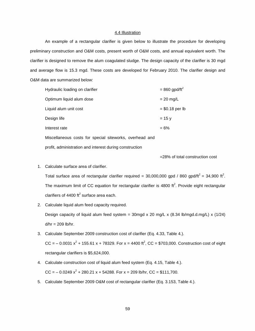
59

4.4 Illustration

An example of a rectangular clarifier is given below to illustrate the procedure for developing

preliminary construction and O&M costs, present worth of O&M costs, and annual equivalent worth. The

clarifier is designed to remove the alum coagulated sludge. The design capacity of the clarifier is 30 mgd

and average flow is 15.3 mgd. These costs are developed for February 2010. The clarifier design and

O&M data are summarized below:

Hydraulic loading on clarifier = 860 gpd/ft2

Optimum liquid alum dose = 20 mg/L

Liquid alum unit cost = $0.18 per lb

Design life = 15 y

Interest rate = 6%

Miscellaneous costs for special siteworks, overhead and

profit, administration and interest during construction

=28% of total construction cost

1. Calculate surface area of clarifier.

Total surface area of rectangular clarifier required = 30,000,000 gpd / 860 gpd/ft2 = 34,900 ft2.

The maximum limit of CC equation for rectangular clarifier is 4800 ft2. Provide eight rectangular

clarifiers of 4400 ft2 surface area each.

2. Calculate liquid alum feed capacity required.

Design capacity of liquid alum feed system = 30mgd x 20 mg/L x (8.34 lb/mgd.d.mg/L) x (1/24)

d/hr = 209 lb/hr.

3. Calculate September 2009 construction cost of clarifier (Eq. 4.33, Table 4.).

CC = – 0.0031 x2 + 155.61 x + 78329. For x = 4400 ft2, CC = $703,000. Construction cost of eight

rectangular clarifiers is $5,624,000.

4. Calculate construction cost of liquid alum feed system (Eq. 4.15, Table 4.).

CC = – 0.0249 x2 + 280.21 x + 54288. For x = 209 lb/hr, CC = $111,700.

5. Calculate September 2009 O&M cost of rectangular clarifier (Eq. 3.153, Table 4.).

60

O&MC = – 0.00003 x2 + 4.2485 x + 7748. For x = 4300 ft2, O&MC = $25,860/y. O&M cost for

eight rectangular clarifiers is $206,880/y.

6. Calculate September 2009 O&M cost of liquid alum feed system (Eq. 3.137, Table 4.).

O&MC = is 2118 x0.293. For x = 209 lb/hr, O&MC = $10,100/y.

7. Update the construction cost of clarifier and alum feed system to February, 2010 (Eq. 2.2).

February 2010 ENR CCI = 8671.77 (Engineering News-Record, 2010). February 2010

construction cost = ($5,624,000 + $111,700) x (8671.77/8585.71) = $5,793,100.

8. Update O&M costs of rectangular clarifier to February, 2010.

September 2009 O&M cost for rectangular clarifier = $206,880/y. Component percent of

electricity, labor and maintenance materials are 3%, 88% and 9% respectively (Eq. 3.30, Table

4.). The September 2009 annual costs of each component are $6210, $182,050, and $18,620

respectively. The updated February 2010 unit price of electricity, and labor are 0.0942/kW.h

(Energy Information Administration, 2010), and $46.57 (Engineering News-Record, 2010)

respectively. February 2010 ENR CCI is 8671.77 (Engineering News-Record, 2010). The updated

February 2010 cost of electricity = $6210/y x (0.0942/0.0981) = $5960/y; labor = $182,050/y x

(46.57/45.82) = $185,030/y; and maintenance materials = $18,620/y x (8671.77/8585.71) =

$18,810/y. Total February 2010 O&M cost of clarifiers = $209,800/y.

9. Update O&M costs of liquid alum feed system to February, 2010.

September 2009 O&M cost for alum feed system = $10,100/y. Component percent of electricity,

labor and maintenance materials are 52%, 45% and 3% respectively (Eq. 3.14, Table 4.). The

September 2009 annual costs of each component are $5250/y, $4550/y, and, $300/y

respectively. The updated February 2010 cost of electricity = $5250/y x (0.0942/0.981) = $5040/y;

labor = $4550/y x (46.57/45.82) = $4620/y; and, maintenance materials = $300/y x

(8671.77/8585.71) = $300/y. Total February 2010 O&M cost of liquid alum feed system =

$9960/y.

61

10. Calculate February 2010 cost of liquid alum feed.

The average plant flow = 15.3 mgd. Annual liquid alum requirement = 15.3 mgd x 20 mg/L x (8.34

lb/mgd.d.mg/L) x 365 d/y = 931,500 lb/y. Annual liquid alum cost in February 2010 = 931,500 lb/y

x $0.18/lb = $167,670/y.

11. Calculate the capital cost.

Special costs are 28 percent of construction cost. Total capital cost = 1.28 x $5,793,100 =

$7,415,200.

12. Calculate the present worth of annual O&M cost, and equivalent annual costs (Eq. 2.4 & 2.5)

The design life of the facility is 15 yrs and interest rate is 6%.

CRF = 0.06/(1 – 1.06)–15 = 0.103.

PW of annual O&M cost = ($209,800 + $9960 + $167,670)/0.103 = $3,761,460.

Project PW = $3,761,460 + $7,415,200 = $11,176,660.

Annual equivalent cost = $11,176,660 x 0.103 = $1,151,200.

4.5 Excel™ Template for Preliminary Cost Estimate of 1 mgd to 200 mgd Water Treatment Plants

An Excel™ template was prepared for preliminary cost estimate of 1 mgd to 200 mgd water

treatment plants. This template is a result of thesis and has been submitted as a supplementary file to the

thesis. It allows the users to enter the design data to obtain desired outputs. The outputs include total

capital costs, operation and maintenance costs, project present worth, annual equivalent worth, and cost

per gallon of water treated. The template contains following spreadsheets:

4.5.1 Project Details

This spreadsheet allows the user to enter basic project design data. The information users can

input are date of estimate, name of the project, project location, design capacity, average plant flow (as

percentage of design capacity), project design life, interest rate, expected inflation rate, current labor

price, current electricity price, current diesel price, current natural gas price, and special costs (general

contractor’s overhead, engineering, land, legal, fiscal, and administrative) as percentage of construction

cost. The user can use either single index or multiple indexes for cost updates. If single index option is

chosen, the user can further select between using ENR Construction Cost Index or ENR Building Cost

Index. The user is asked to enter current value of single index selected. If multiple index option is

62

selected, the user is asked to enter current value of all applicable indexes which are ENR Skilled Labor

Index, BLS General Purpose Machinery Index, BLS Concrete Ingredients Index, BLS Steel Mill Products

Index, BLS Valves and Fittings Index, BLS Electrical Machinery and Equipment Index, ENR Building Cost

Index, and BLS Producer Price Index for Commodity.

4.5.2 Unit Operation and Processes

In this spreadsheet, the users enter design criteria of each treatment unit that is part of the

process train being evaluated. Current construction and O&M costs are automatically calculated through

built in equations and update factors. The equations presented in Tables 10 & 12 are comprehensively

used as built in equations. Update factors are calculated from the indexes entered by the user.

Construction and O&M costs of each treatment unit selected by the user as required are presented as

output.

4.5.3 Summary of Capital Costs

This spreadsheet presents summary of the capital costs obtained from the design criteria entered

by the user. The users can also input self calculated other capital costs not covered by the built in

equations of the template.

4.5.4 Summary of O&M Costs

This spreadsheet presents summary of the O&M costs obtained from the design criteria entered

by the user. The users can also input self calculated O&M costs not covered by the built in equations of

the template. Most of the chemical costs are calculated through built in equations as well. However, the

chemical costs not covered in “Unit Operation and Processes” spreadsheet must be entered separately in

this spreadsheet.

4.5.5 Present & Annual Value

This spreadsheet presents final output of the template. Annual cost for each year is presented in

tabular form. Present value of the project, annual equivalent worth, and cost per gallon of water treated is

presented.

63

4.6 Chapter Summary

The cost equations presented in Tables 4.1, 4.2, 4.3 and 4.4 are essentially the results of this

thesis. Illustration to show steps to utilize these equations to calculate present value and annual

equivalent worth of a project was presented in this chapter. Excel™ template for estimation of capital and

O&M costs of water treatment plants was also described.

64

CHAPTER 5

CONCLUSIONS AND RECOMMENDATIONS

5.1 Conclusions

Generalized construction, and operation and maintenance cost equations are convenient way to

develop preliminary cost estimates of water treatment plants during the planning phase. The construction

and O&M equations presented in this thesis are quicker to use than the cost curves. Probability of human

error is considerably decreased when cost equations are used instead of cost curves. If short time interval

is involved, the construction and O&M costs updating procedure using single ENR cost index can be

used. Designers may use same approach presented in this paper but with other cost indexes if desired.

The total present worth and equivalent annual costs are used to evaluate and compare the

economics of different alternatives, and to arrange for project funding and to secure engineering design

services.

The cost estimates developed from these equations are only preliminary estimates and do not

represent the accutate cost estimate of the project. Actual construction costs of the projects heavily

depend on the site conditions, weather, competetion among bidders and suppliers, and general local and

nationwide economic conditions. Therefore, detailed estimates of construction, and operation and

maintenance costs cannot be generalized and must be developed for each specific project. Design details

and cost estimates based on quantities of materials, equipment, and labor should be used to develop

detailed cost estimate of the project.

5.2 Recommendations for Future Research

The users of the cost equations presented in this thesis must be aware of the cost components

included in the equations. The cost components included in these equations are general. However,

detailed estimate of project costs are specific and cannot be generalized. Therefore, use of these

equations is recommended for evaluation of alternatives and arrangement of funds. The detailed estimate

of project costs require quantity take-offs of detailed design and actual prices provided by manufacturers,

suppliers and subcontractors.

65

It is recommended that the construction & O&M costs are updated at intervals of at five to eight

years and new set of equations be presented in this time interval. Other available cost indexes (presented

in Appendix A) should also be evaluated to see which index best fits to predict construction and O&M

costs of water treatment plants. It is essential to compare the result of the equations presented in this

thesis with the actual cost data obtained from the industry. This comparison will help in evaluation of

usefulness of cost equations and indexes in preliminary estimates of water treatment plant construction,

and O&M costs.

66

APPENDIX A

COST AND LOCATION INDEXES FOR THE UNITED STATES

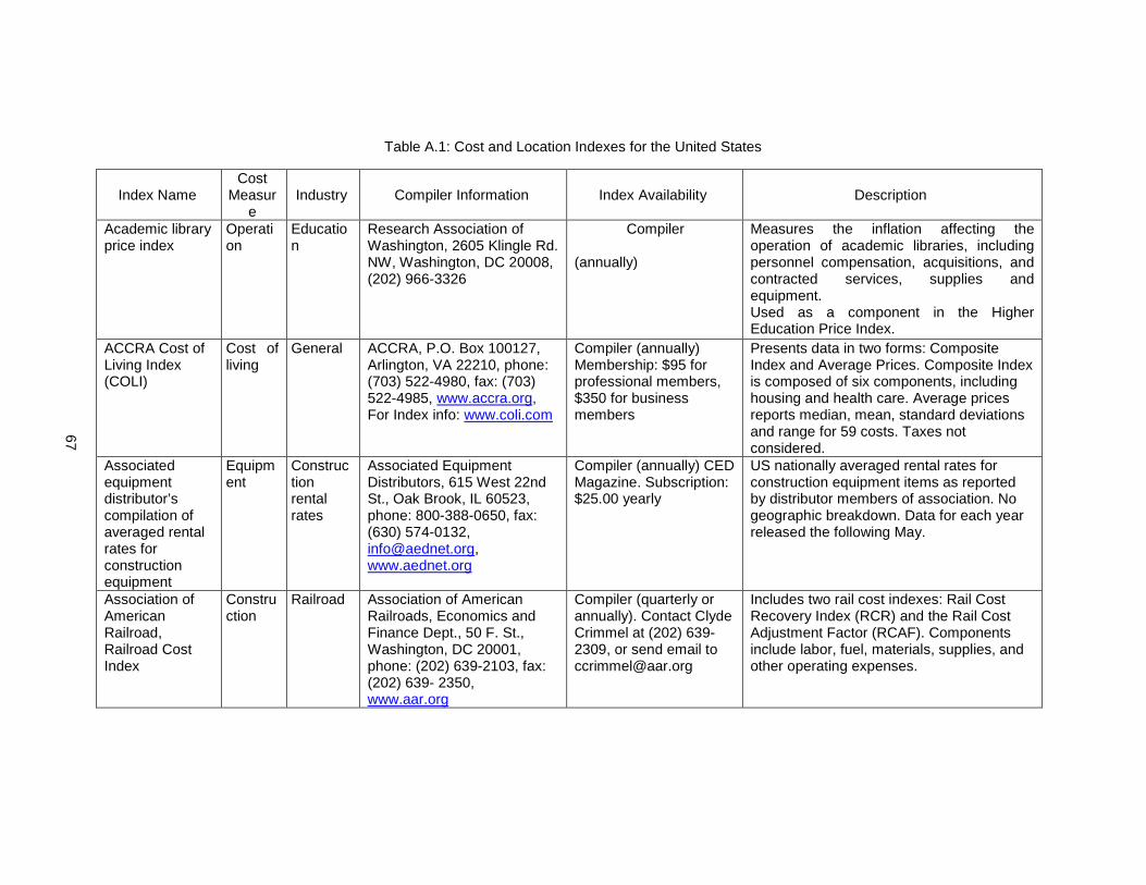
67

Table A.1: Cost and Location Indexes for the United States

Index Name Cost

Measure

Industry Compiler Information Index Availability Description

Academic library price index

Operation

Education

Research Association of Washington, 2605 Klingle Rd. NW, Washington, DC 20008, (202) 966-3326

Compiler

(annually)

Measures the inflation affecting the operation of academic libraries, including personnel compensation, acquisitions, and contracted services, supplies and equipment. Used as a component in the Higher Education Price Index.

ACCRA Cost of Living Index (COLI)

Cost of living

General ACCRA, P.O. Box 100127, Arlington, VA 22210, phone: (703) 522-4980, fax: (703) 522-4985, www.accra.org, For Index info: www.coli.com

Compiler (annually) Membership: $95 for professional members, $350 for business members

Presents data in two forms: Composite Index and Average Prices. Composite Index is composed of six components, including housing and health care. Average prices reports median, mean, standard deviations and range for 59 costs. Taxes not considered.

Associated equipment distributor’s compilation of averaged rental rates for construction equipment

Equipment

Construction rental rates

Associated Equipment Distributors, 615 West 22nd St., Oak Brook, IL 60523, phone: 800-388-0650, fax: (630) 574-0132, [email protected], www.aednet.org

Compiler (annually) CED Magazine. Subscription: $25.00 yearly

US nationally averaged rental rates for construction equipment items as reported by distributor members of association. No geographic breakdown. Data for each year released the following May.

Association of American Railroad, Railroad Cost Index

Construction

Railroad Association of American Railroads, Economics and Finance Dept., 50 F. St., Washington, DC 20001, phone: (202) 639-2103, fax: (202) 639- 2350, www.aar.org

Compiler (quarterly or annually). Contact Clyde Crimmel at (202) 639-2309, or send email to [email protected]

Includes two rail cost indexes: Rail Cost Recovery Index (RCR) and the Rail Cost Adjustment Factor (RCAF). Components include labor, fuel, materials, supplies, and other operating expenses.

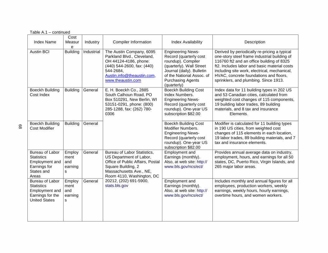
68

Table A.1 – continued

Index Name Cost

Measure


Austin BCI Building Industrial The Austin Company, 6095 Parkland Blvd., Cleveland, OH 44124-4186, phone: (440) 544-2600, fax: (440) 544-2684, [email protected], www.theaustin.com

Engineering News-Record (quarterly cost roundup). Compiler (quarterly). Wall Street Journal (daily). Bulletin of the National Assoc. of Purchasing Agents (quarterly)

Derived by periodically re-pricing a typical one-story steel frame industrial building of 116760 ft2 and an office building of 8325 ft2. Includes labor and basic material costs including site work, electrical, mechanical, HVAC, concrete foundations and floors, sprinklers, and plumbing. Since 1913.

Boeckh Building Cost Index

Building General E. H. Boeckh Co., 2885 South Calhoun Road, PO Box 510291, New Berlin, WI 53151-0291, phone: (800) 285-1288, fax: (262) 780- 0306

Boeckh Building Cost Index Numbers. Engineering News-Record (quarterly cost roundup). One-year US subscription $82.00

Index data for 11 building types in 202 US and 53 Canadian cities, calculated from weighted cost changes of 115 components, 19 building labor trades, 89 building materials, and 8 tax and insurance

Elements.

Boeckh Building Cost Modifier

Building General Boeckh Building Cost Modifier Numbers. Engineering News-Record (quarterly cost roundup). One-year US subscription $82.00

Modifier is calculated for 11 building types in 190 US cities, from weighted cost changes of 115 elements in each location, 19 labor trades, 89 building materials, and 7 tax and insurance elements.

Bureau of Labor Statistics Employment and Earnings for States and Areas

Employment and earnings

General Bureau of Labor Statistics, US Department of Labor, Office of Public Affairs, Postal Square Building, 2 Massachusetts Ave., NE, Room 4110, Washington, DC 20212, (202) 691-5900, stats.bls.gov

Employment and Earnings (monthly). Also, at web site: http:// www.bls.gov/ncs/ect/

Provides annual average data on industry, employment, hours, and earnings for all 50 states, DC, Puerto Rico, Virgin Islands, and 265 major labor areas.

Bureau of Labor Statistics Employment and Earnings for the United States

Employment and earnings

General Employment and Earnings (monthly). Also, at web site: http:// www.bls.gov/ncs/ect/

Includes monthly and annual figures for all employees, production workers, weekly earnings, weekly hours, hourly earnings, overtime hours, and women workers.

69


Index Name Cost

Measure


Bureau of Labor Statistics Employment Cost Index for Private Industry Workers

Wages and salaries, benefits, and compensation

General Bureau of Labor Statistics, Office of Compensation and Working Conditions, Suite 4175, 2 Massachusetts Ave., NE, Washington, DC 20212, phone: (202) 691-6199, fax: (202) 691-6647, stats.bls.gov

For the indexes: http://stats.bls.gov/ news.release/eci.toc.htm

Provides semi-annual wages and salaries, benefits, and compensation indexes for private industry workers, categorized by industry and occupational groups. Not seasonally adjusted.

Bureau of Labor Statistics Producer Price Index – Construction Machinery and Equipment

Producer price

Construction machinery and equipment

Producer prices and price index (monthly)

Nine categories of construction equipment and machinery, including Portable Air Compressors and Parts. Based on direct price reporting of typical transaction and list prices generally from manufacturer to distributor. Monthly, since January 1947.

Bureau of Reclamation

Construction

General Bureau of Reclamation, Denver Federal Center, P.O. Box 25007, 5th Ave. and Kippling, Denver, CO 80225, phone: (303) 445-2784, www.usbr.gov/

Compiler (quarterly); Engineering News-Record (bi-annually). Publications also at bookstore.gpo.gov/index.html

Compiler’s release covers 34 types of dam and water projects. ENR publishes the Bu-Rec’s general property index that measures costs for office and maintenance buildings associated with its projects. Website includes construction quarterly indexes for 36 types of structures.

Chemical Engineering Plant Cost Index (CEPCI)

Construction

Plant (chemical)

Chemical Engineering, McGraw Hill, Inc., 1221 Avenue of the Americas, New York, NY 10020, phone: (212) 512-2000, www.mcgraw-hill.com, Also, http://www.che.com/pindex/

Chemical Engineering (biweekly) annual subscription $495; US Bureau of Labor Statistics survey of hourly earnings (monthly); BLS National Survey of Professional, Administrative, Technical, and Clerical Pay

Specifically for a chemical process plant, but used throughout the process industry. Cost components include equipment, machinery, labor, building materials, engineering, and supervision costs. Productivity corrections for wages/salaries and engineering services.

70


Index Name Cost

Measure


Consumer Price Index

Goods Consumer

Bureau of Labor Statistics, Division of Consumer Prices and Price Indexes, Suite 3130, 2 Massachusetts Ave., NE, Washington, DC 20212, (202) 691-7000, stats.bls.gov

BLS press release (initial). Consumer Prices and Price Index (monthly). BLS supplements (annually). More info at http://www.bls.gov/cpi/

Measures average changes in prices of about 400 goods and services bought by wage earners and clerical workers, both families and single persons. Weightings based on periodic surveys. Annually and monthly, since 1913.

Dept. of Commerce Composite CCI

Construction

General Bureau of the Census, Construction Statistics Division, US Dept. of Commerce, Washington, DC 20233, www.census.gov

Construction Reports (monthly); Construction Review (bi-monthly); Engineering News-Record (quarterly cost roundup); or get historical data (1964–2003) at: www.census.gov/pub/const/C30/indexes.html

Combination of various cost indexes weighted monthly to the current relative importance of major classes of construction. Publishes two construction related indexes. First, a composite fixed-weight index is a ratio of the annual value of new construction put in place in current dollars to comparable values in 1992. This index reflects only a change in price. The second reflects changes in prices but also changes in the composition of value put in place. This reflects market conditions as well as price. Both published monthly.

Dept of Commerce Schedule of Annual Indexes for Carriers by Railroad

Construction

Railroad Interstate Commerce Div., Bureau of the Accounts, Washington, DC 20423

Compiler (annually) A series of indexes that trends reproduction cost changes in railroad property and equipment. Cost components include grading, tunnels, bridges, ties, rail, locomotives, and freight cars. Indexes applicable to national average only. Since 1915.

Dodge Building Cost Index

Construction

General Marshall and Swift, 1617 Beverly Blvd, Los Angeles. CA 90026, phone: (800) 526-2756, (800) 262-4729, Or, (800) 393–6343, http://www.marshallswift. comwww.marshallswift.com

Dodge Unit Cost Guide Components include labor (22 trades), material, and equipment costs includes crew sizes, productivity rates, individual prices for hard-to-find items, and location factors for 1000 regions in US and Canada included. Compiled quarterly.

71


Index Name Cost

Measure


Engineering News- Record Building Cost Index

Construction —structure cost dominates

General Engineering News- Record, McGraw-Hill, Inc., Two Penn Plaza, New York, NY 10121-2298, phone: (212) 904–3507, www.enr.com

Engineering News- Record (weekly). One year US subscription $82.00

Applicable to structure construction. Obtained by weekly re-pricing of a hypothetical block of construction in 20 US cities. Includes skilled labor, structural steel shapes, cement and lumber.

Engineering News- Record Common Labor Index

Labor Wage-rate


Data obtained by averaging current wage rates for common labor on buildings and other construction and by averaging rates for bricklayers, carpenters, and structural ironworkers in 20 US cities.

Engineering News- Record Materials Cost Index

Materials

General Engineering News- Record (weekly). One year US subscription $82.00

Indexes of structural steel, portland cement, and lumber materials.

Engineering News- Record Skilled Labor Index

Labor Wage-rate


Covers skilled labor wage rates, based on base rates and fringe benefits, in dollars per hour for 20 cities in the US. Index also tracks union wages, plus fringe benefits for certain workers.

Federal Highway Administration (FHWA) Construction Bid Price Index

Construction

Highway-Federal

Highway-Federal US Department of Transportation, Federal Highway Administration, 400 7th Street, SW, Washington, DC 20590, www.fhwa.dot.gov

Price Trends for Federal-Aid Highway Construction (quarterly); Survey of Current Business (monthly); Engineering News-Record (quarterly cost roundup); Highway and heavy construction (quarterly); Highway statistics (annually)

Tracks cost of current prices for base period quantities. Derived from average unit bid prices for excavation, surfacing, and structures. Restructured when necessary. Quarterly since 1972. Annually, since 1962.

72


Index Name Cost

Measure


Fru-Con BCI Building Industrial Fru-Con Corporation, 15933 Clayton Rd., P.O. Box 100, Ballwin (St. Louis), MO 63011, phone: 1-800-FRUCON, or (636) 391–6799, fax: (636) 391-4513, [email protected] , www.frucon.com

Compiler (monthly) Based on an average industrial building in St. Louis region. Components include current labor and materials costs (fridges, concrete mortar, clay, lumber, plastics, metals, paint, and glass). Weightings adjusted if needed.

Handy-Whitman of Public Utility Construction Cost Index

Construction

Public utility

Whitman, Requardt and Associates, 801 South Caroline Street, Baltimore, MD 21231, phone: (410) 235-3450, fax: (410) 243-5716, [email protected] , www.wrallp.com

Compiler (annually) Treats construction costs separately for electric, gas, water, and telephone utility construction. Weightings and components revised when needed. For 6 US geographical regions in 48 contiguous states. Since 1912. There is also an index for a reinforced concrete building.

Higher Education Price Index

Operation

Education

Research Association of Washington, 2605 Klingle Rd. NW, Washington, DC 20008

Compiler (annually) Measures the price level of goods and services colleges and universities purchase for their current education operations.

JOC-ECRI Industrial Price Index

Raw materials

Industrial Economic Cycle Research Institute, 420 Lexington Avenue, Suite 1645, New York, NY 10170, phone: (212) 557-7788, fax: (212) 557-9874, www.businesscycle.com

Compiler. Journal of Commerce: www.joc.com

This index is designed to yield a cyclical leading indicator of the inflation cycle. Made of 18 components divided into 4 sub-indexes: Petroleum products, Metals, Textiles and Miscellaneous. Created in 1986 and revised in 1994.

Lee Saylor BCI Building General Saylor Publications, Inc., 9420 Topanga Canyon Blvd., Suite 203, Chatsworth, CA 91311, phone: (800) 624-3352, fax: (818) 718-8024, [email protected], www.saylor.com

Compiler (monthly). Construction Costs: 74.95 per copy Indexes (from 1967 to 2005): www.saylor.com/indexes.htm

Components include 9 types of labor and 23 materials costs quoted in 20 cities. A Labor-Material Cost Index weighted at 54% labor and 46% materials. Subcontractor Index also available for 21 materials. Monthly. Lee Saylor went bankrupt in 1995. Index now compiled by Saylor Publications, Inc.

73


Index Name Cost

Measure


Marshall and Swift Industrial Equipment Cost Index

Equipment

General Marshall and Swift, 1617 Beverly Blvd, Los Angeles. CA 90026, phone: (800) 526-2756, www.marshallswift.com

Chemical Engineering. Marshall Valuation Service (monthly). Valuation Book (quarterly)

Represents a composite of the equipment costs of an entire plant based on a national average. Covers 48 industries with the general average for all. Since 1913. Also available for 18 Canadian cities.

Marshall and Swift Commercial Building Estimator Software

Building General Commercial Estimator. For more information: www.swiftestimator.com/ce.asp

Allows user to quickly estimate costs on nearly 250 commercial, industrial, retail, agricultural or institutional buildings including all classes, sizes, shapes and quality levels.

Marshall and Swift Building Cost Index

Building Industrial, appraisal

Marshall Valuation Service (monthly). Valuation Book (quarterly)

Index is an average of 100 US cities combined into various regional, district, and national indexes. Tracks costs of 5 types of buildings in various parts of US: fire-proof steel, reinforced concrete, masonry, wood, and pre-engineering steel frames. Components include materials, equipment and labor. Since 1901.

Means Building Construction Cost

Construction

General R. S. Means Company, Inc., PO Box 800, 63 Smiths Lane, Kingston, MA 02364-9988, phone: (800) 334-3509, fax: (800) 632-6732, www.rsmeans.com

CostWorks software. Allows user to access industry-standard Means construction costs. $142.95 (2005) and $154.95 (2006)

Tracks construction costs for 16 components in 305 US cities and Canadian cities and 50 components for New York, Houston, LA, Chicago, and Boston. National averages for 30 largest US cities included.

Means Assemblies Cost

Complete build-ing Ass-emblies

General Tracks assemblies’ costs for 16 components in 305 US cities and Canadian cities. National averages for 30 largest US cities included.

Means Concrete & Masonry Cost

Construction

General Cost facts for virtually all concrete/masonry estimating needs, from complicated formwork to various sizes and face finishes of brick and block. Unit cost section contains more than 8,500 selected entries.

74


Index Name Cost

Measure


Means Electrical Cost

Construction

General R. S. Means Company, Inc., PO Box 800, 63 Smiths Lane, Kingston, MA 02364-9988, phone: (800) 334-3509, fax: (800) 632-6732, www.rsmeans.com

CostWorks software. Allows user to access industry-standard Means construction costs. $142.95 (2005) and $154.95 (2006)

More than 15,000 unit and systems costs with design tables.

Means Facilities Construction Cost

Construction

General CostWorks software. Allows user to access industry-standard Means construction costs. $329.95 (2005) and $356.95 (2006)

Provides costs associated with maintenance, construction and renovation of commercial, industrial, municipal, and institutional properties.

Nelson-Farrar Refinery Construction Cost Index

Construction

Refinery Oil and Gas Journal, 1421 S. Sheridan Rd., Tulsa, OK 74112, phone:(918) 832–9301, FAX: (918) 831–9776, ogj.pennnet.com/cd_anchor_home/

Oil and Gas Journal Components include process equipment, electrical machinery, instrumentation, heat exchangers, materials, and labor costs. Since 1926.

Nelson-Farrar Refinery Operating Cost Index

Operating

Refinery Oil and Gas Journal, 1421 S. Sheridan Rd., Tulsa, OK 74112, phone:(918) 832–9301, fax: (918) 831–9776, ogj.pennnet.com/cd_anchor_home/

Oil and Gas Journal Measures inflation effects on refinery operating costs. Components include fuel, labor, chemicals, maintenance, and investment costs.

New Residential Construction Index

Construction

Housing construction

Bureau of the Census, Residential Construction Branch, 4700 Silver Hill Road, Washington, DC 20233, (301) 763–5160, www.census.gov

Information on web site http://www.census.gov/const/www/newresconstindex.html

Provides index including building permits, housing starts and housing completions. By US and regions, this index provides quarterly starts and completions.

Producer Price Index

Goods Producer Bureau of Labor Statistics, Producer Price Index, Suite 3840, 2 Massachusetts Ave., NE, Washington, DC 20212, (202) 691- 7705, stats.bls.gov

BLS press release (initial). Producer Prices and Price Index (monthly). BLS supplements (annually).

Covers all commodities produced or imported and sold in US primary markets. Listed separately and by groups, such as Crude Materials and Finished Goods. Based on sales of large lots in the primary market, reported by survey. Since 1890.

75


Index Name Cost

Measure


Research and Development Price Index

Goods Education


Compiler (annually)

Measures the inflation affecting university research funding and expenditures.

Richardson Construction Cost Trend Reporter

Labor Construction

Richardson Engineering Services, Inc., PO Box 9103, Mesa. AZ 85214- 9103, phone: (480) 497-2062, fax: (480) 497-5529

Compiler (semi-annually)

Tracks average labor rates for various types of construction crews. Averaged for the entire US. Enables detailed labor cost estimation for construction projects.

Richardson International Construction Factors

Location factors

Construction

Richardson Engineering Services, Inc., PO Box 9103, Mesa. AZ 85214-9103, phone: (480) 497-2062, FAX: (480) 497-5529

Compiler (semi-annually)

Provides location factors based on typical process plants for 14 major process industry locations around the world.

School Price Index

Operation

Education


Compiler (annually) Measures the price level of goods and services purchased by primary and secondary education institutions.

United States Import and Export Price Index

Imported and exported goods

General Bureau of Labor Statistics, Office of International Prices, Suite 3955, 2 Massachusetts Ave., NE, Washington, DC 20212, phone: (202) 691-7101, fax: (202) 691-7179, stats.bls.gov

For the indexes: stats.bls.gov/mxp/home.htm

Provides indexes of goods or services purchased from abroad by US residents (imports) or sold to foreign buyers by US residents (exports). Monthly indexes by locality of origin are available

US Periodical Price Index

Periodicals

General http://www.ala.org/ American Libraries (annual)

Includes indexes that track change in annual subscription of periodicals. Also, this has breakdowns by subject categories and ranks by subscription price increases .

Source: Remer et al. (2008)

76

APPENDIX B

CONTROLLED SINGLE INDEX UPDATES AT INTERVAL OF 8 AND 10 YEARS

77

Figure B.1: Construction Costs of 3600 ft2 Rectangular Clarifier, Updated Using Single Index, Multiple Indexes, and Controlled Single Index, 8 yr Interval

Figure B.2: Construction Costs of 50 mgd Gravity Filtration Structure, Updated Using Single Index, Multiple Indexes, and Controlled Single Index, 8 yr Interval

$0

$100,000

$200,000

$300,000

$400,000

$500,000

$600,000

$700,000

1977 1987 1997 2007

Up

dat

ed C

on

stru

ctio

n C

ost

Year

Single Index

Multiple Indexes


$0

$1,000,000

$2,000,000

$3,000,000

$4,000,000

$5,000,000

$6,000,000

$7,000,000

1977 1987 1997 2007

Up

dat

ed C

on

stru

ctio

n C

ost

Year

Single Index

Multiple Indexes


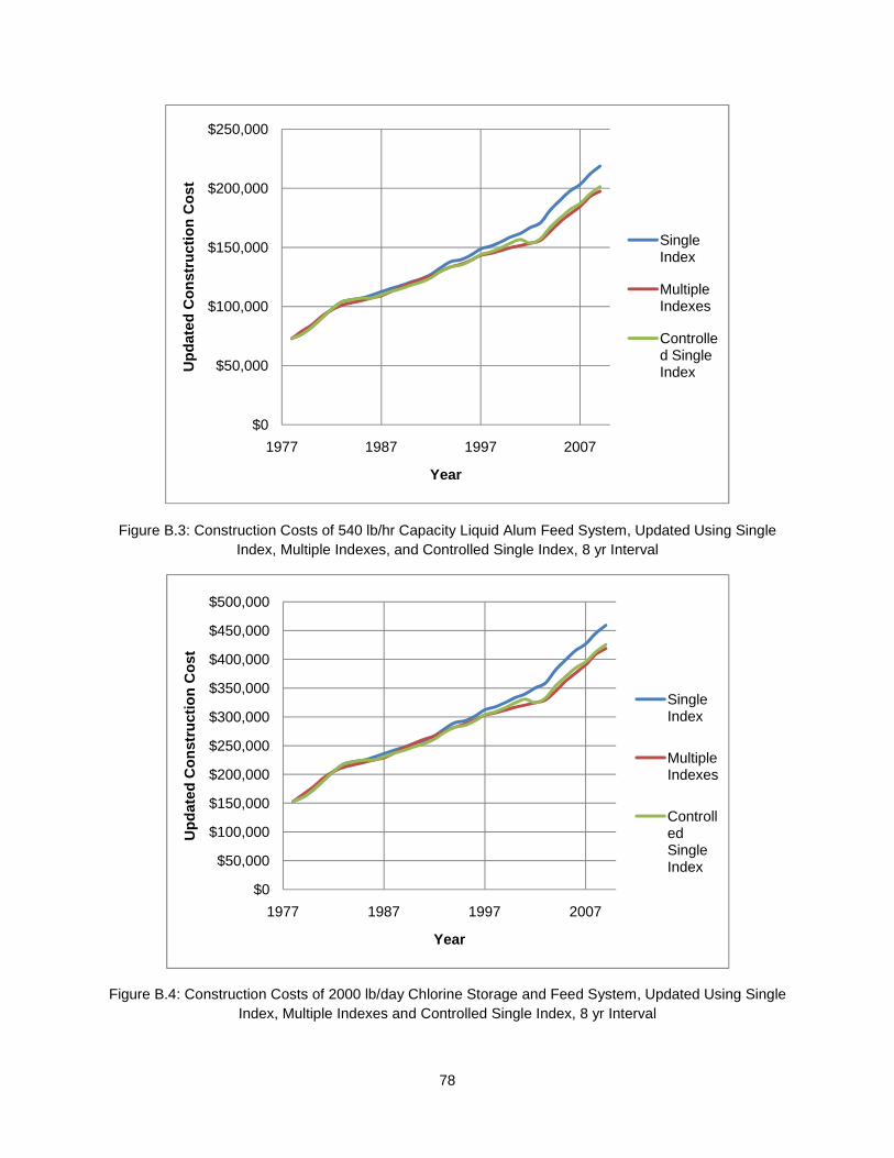
78

Figure B.3: Construction Costs of 540 lb/hr Capacity Liquid Alum Feed System, Updated Using Single Index, Multiple Indexes, and Controlled Single Index, 8 yr Interval

Figure B.4: Construction Costs of 2000 lb/day Chlorine Storage and Feed System, Updated Using Single Index, Multiple Indexes and Controlled Single Index, 8 yr Interval

$0

$50,000

$100,000

$150,000

$200,000

$250,000

1977 1987 1997 2007

Up

dat

ed C

on

stru

ctio

n C

ost

Year

Single Index

Multiple Indexes


$0

$50,000

$100,000

$150,000

$200,000

$250,000

$300,000

$350,000

$400,000

$450,000

$500,000

1977 1987 1997 2007

Up

dat

ed C

on

stru

ctio

n C

ost

Year

Single Index

Multiple Indexes


79

Figure B.5: Construction Costs of 1400 ft2 Filter Area Capacity Air-Water Backwash, Updated Using Single Index, Multiple Indexes, and Controlled Single Index, 8 yr Interval

Figure B.6: Construction Costs of 3600 ft2 Rectangular Clarifier, Updated Using Single Index, Multiple Indexes, and Controlled Single Index, 10 yr Interval

$0

$100,000

$200,000

$300,000

$400,000

$500,000

$600,000

1977 1987 1997 2007

Up

dat

ed C

on

stru

ctio

n C

ost

Year

Single Index

Multiple Indexes


$0

$100,000

$200,000

$300,000

$400,000

$500,000

$600,000

$700,000

1977 1987 1997 2007

Up

dat

ed C

on

stru

ctio

n C

ost

Year

Single Index

Multiple Indexes


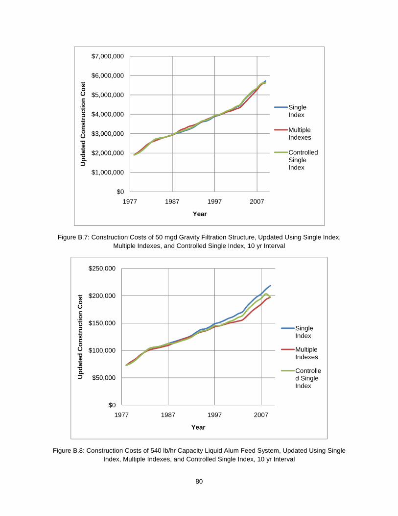
80

Figure B.7: Construction Costs of 50 mgd Gravity Filtration Structure, Updated Using Single Index, Multiple Indexes, and Controlled Single Index, 10 yr Interval

Figure B.8: Construction Costs of 540 lb/hr Capacity Liquid Alum Feed System, Updated Using Single Index, Multiple Indexes, and Controlled Single Index, 10 yr Interval

$0

$1,000,000

$2,000,000

$3,000,000

$4,000,000

$5,000,000

$6,000,000

$7,000,000

1977 1987 1997 2007

Up

dat

ed C

on

stru

ctio

n C

ost

Year

Single Index

Multiple Indexes


$0

$50,000

$100,000

$150,000

$200,000

$250,000

1977 1987 1997 2007

Up

dat

ed C

on

stru

ctio

n C

ost

Year

Single Index

Multiple Indexes


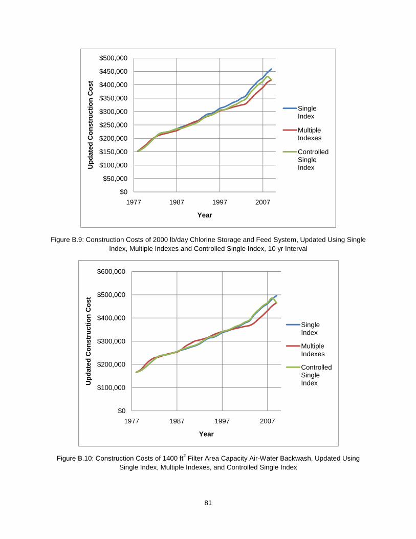
81

Figure B.9: Construction Costs of 2000 lb/day Chlorine Storage and Feed System, Updated Using Single Index, Multiple Indexes and Controlled Single Index, 10 yr Interval

Figure B.10: Construction Costs of 1400 ft2 Filter Area Capacity Air-Water Backwash, Updated Using Single Index, Multiple Indexes, and Controlled Single Index

$0

$50,000

$100,000

$150,000

$200,000

$250,000

$300,000

$350,000

$400,000

$450,000

$500,000

1977 1987 1997 2007

Up

dat

ed C

on

stru

ctio

n C

ost

Year

Single Index

Multiple Indexes


$0

$100,000

$200,000

$300,000

$400,000

$500,000

$600,000

1977 1987 1997 2007

Up

dat

ed C

on

stru

ctio

n C

ost

Year

Single Index

Multiple Indexes


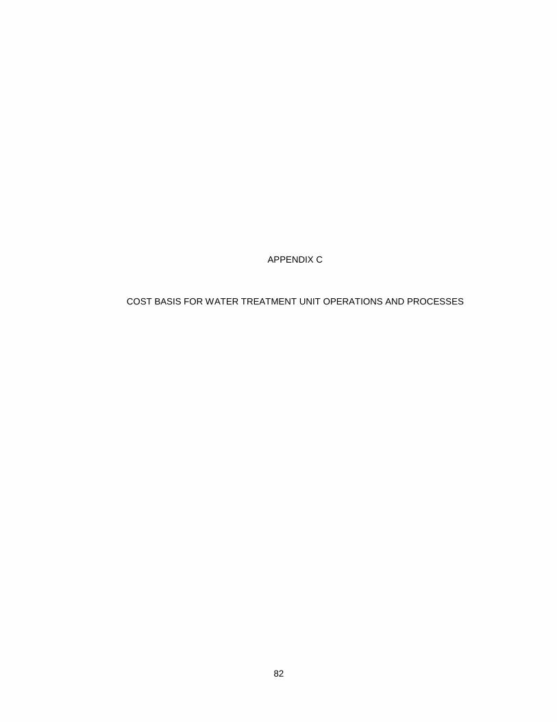
82

APPENDIX C

COST BASIS FOR WATER TREATMENT UNIT OPERATIONS AND PROCESSES

83

Table C.1: Cost Basis for Water Treatment Unit Operations and Processes

Treatment Units Construction Cost Operation & Maintenance Cost Raw Water Pumping Raw Water Pumping Facilities

Includes pumps, valves and manifold piping, and electrical equipment and instrumentation. Wet well and housing are not included.

Energy costs include pumps and motors. Maintenance material cost includes repair parts for pumps and motors, valves, and electrical starters and controls. Labor cost includes O&M of pumps and motors, valves, and electrical controls.

TDH = 30 ft.

TDH = 100 ft.

Diffused Aeration Basin

Includes open rectangular reinforced concrete basins, direct drive centrifugal compressors, and porous diffusers.

Energy cost includes continuous operation of direct drive centrifugal air compressors. Maintenance material costs include lubricants, replacement components for air compressors, and air diffusion equipment. Labor costs include maintenance of air compressors, air piping, valves, and diffusers and for maintenance of aeration basins.

Aeration Towers Includes rectangular aeration towers with 16-ft of PVC media and overall tower height of 22-ft, reinforced concrete basin support, and electrically driven induced-draft fans with fan stacks and drift eliminators.

Energy cost includes continuous operation of induced draft fan. Maintenance material costs include replacement of packing media, lubricants for fans and motors, and other miscellaneous items. Labor costs include fan and motor maintenance, weekly housing of distributing nozzles and media to remove slime growths, and occasional repair or replacement of damaged packaged media.

Coagulation, Precipitation, and Flocculation Liquid Alum Feed System

Includes uncovered (indoor for small installations) or covered (and vented with insulation and heating for larger installations) fiber glass reinforced polyester (FRP) tanks for 15 days storage, dual-head metering pumps, standby metering pump, 150 ft 316 stainless steel pipe to convey liquid alum, and miscellaneous fittings and valves for each metering pump.

Energy costs include solution mixers, feeder operation, building lighting, ventilation, heating, and heating for outdoor storage tanks (large liquid feed installations). Maintenance material costs are based on 3% of manufactured equipment cost. Alum costs are not included. Labor costs include chemical loading, routine O&M of feeding equipment, and alum unloading.

Dry Alum Feed System

Based on use of commercial dry alum with a density of 60 lb/ft3, Includes mild steel storage hoppers for 15 days dry alum storage, dust collectors, volumetric feeders for small installations and mechanical weigh belt feeders for large installations, solution tanks located directly beneath storage hoppers, and dual-head diaphragm metering pumps.

84

Table C.1 – Continued Treatment Units Construction Cost Operation & Maintenance Cost

Ferrous Sulfate Feed Systems

Based on use of FeSO4.7H2O with density of 64 lb/ft3. Includes indoor MS storage hoppers for 15 days storage, hoppers, volumetric feeders/mechanical weigh belt feeders, dual-head diaphragm metering pumps, and housing.

Energy costs include solution mixers, feeder operation, building lighting, ventilation, and heating. Maintenance material costs are based on 3% of manufactured equipment cost. Labor costs include chemical unloading, and routine O&M.

Ferric Sulfate Feed Systems

Based on use of Fe(SO4)3.3H2O with density of 80 lb/ft3. Includes indoor MS storage hoppers for 15 days storage, hoppers, volumetric feeders/mechanical weigh belt feeders, dual-head diaphragm metering pumps, and housing.

Energy costs include solution mixers, feeder operation, building lighting, ventilation, and heating. Maintenance material costs are based on 3% of manufactured equipment cost. Labor costs include chemical unloading, and routine O&M.

Polymer Feed Systems

Based on use of dry polymers, fed manually to a storage hopper located on the chemical feeder. Includes chemical feed equipment. No standby or redundant equipment is provided.

Energy costs include feeder and metering pump, and building energy requirements. Maintenance material costs are based on 3% of manufactured equipment and pipe/valve costs. Labor costs include unloading, routine operation and maintenance of chemical feeder and solution metering pump.

Sulfuric Acid Feed Systems

Includes storage tank, metering pump (with standby pump), and FRP tanks for outside storage for 15 days or indoor building area required for storage in drums.

Energy costs include metering pump and building energy for indoor storage. Maintenance material costs are 3% of equipment cost. Labor costs include unloading chemical and O&M for metering pumps.

Sodium Hydroxide Feed Systems

For less than 200 lb/day (dry NaOH) includes a volumetric feeder, two day tanks - mixing and feeding, and pipes and valves. Each tank includes a mixer and a dual-head metering pump. For more than 200 lb/day, includes indoor FRP tanks for 15 days of storage, dual-head metering pumps, and a standby metering pump.

Energy costs include volumetric feeder, mixer, and metering pump. Maintenance material costs are 3% of equipment cost, excluding tanks. Labor costs include unloading chemical and O&M for dual-metering pumps.

Rapid Mix, G = 300 /s Includes reinforced concrete basins (common wall construction for multiple basins), vertical shaft, variable speed turbine mixers, paddle and TEFC motors.

Energy costs are based on motor horsepower. Maintenance material cost includes oil for the gearbox drive unit. Labor costs include jar testing, routine operation and maintenance, oil change, draining, inspection, and cleaning.

Rapid Mix, G = 600 /s

Rapid Mix, G = 900 /s

Flocculation Systems

Includes rectangular-shaped, 12 ft deep reinforced concrete structures, flocculators, manufactured equipments.

Energy costs include motor and mechanism. Maintenance material costs are based on 3% of manufactured equipment cost. Labor costs include O&M of basins, and oil change.

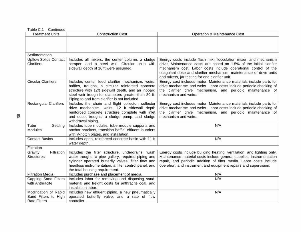
85


Sedimentation Upflow Solids Contact Clarifiers

Includes all mixers, the center column, a sludge scraper, and a steel wall. Circular units with sidewall depth of 16 ft were assumed.

Energy costs include flash mix, flocculation mixer, and mechanism drive. Maintenance costs are based on 1.5% of the initial clarifier mechanism cost. Labor costs include operational control of the coagulant dose and clarifier mechanism, maintenance of drive units and mixers, jar testing for one clarifier unit.

Circular Clarifiers Includes center feed clarifier mechanism, weirs, baffles, troughs, a circular reinforced concrete structure with 12ft sidewall depth, and an inboard steel weir trough for diameters greater than 80 ft. Piping to and from clarifier is not included.

Energy cost includes motor. Maintenance materials include parts for drive mechanism and weirs. Labor costs include periodic checking of the clarifier drive mechanism, and periodic maintenance of mechanism and weirs.

Rectangular Clarifiers Includes the chain and flight collector, collector drive mechanism, weirs, 12 ft sidewall depth reinforced concrete structure complete with inlet and outlet troughs, a sludge pump, and sludge withdrawal piping.

Energy cost includes motor. Maintenance materials include parts for drive mechanism and weirs. Labor costs include periodic checking of the clarifier drive mechanism, and periodic maintenance of mechanism and weirs.

Tube Settling Modules

Includes tube modules, tube module supports and anchor brackets, transition baffle, effluent launders with V-notch plates, and installation.

N/A

Contact Basins Includes open, reinforced concrete basin with 11 ft water depth.

N/A

Filtration Gravity Filtration Structures

Includes the filter structure, underdrains, wash water troughs, a pipe gallery, required piping and cylinder operated butterfly valves, filter flow and headloss instrumentation, a filter control panel, and the total housing requirement.

Energy costs include building heating, ventilation, and lighting only. Maintenance material costs include general supplies, instrumentation repair, and periodic addition of filter media. Labor costs include operation, and instrument and equipment repairs and supervision.

Filtration Media Includes purchase and placement of media. N/A Capping Sand Filters with Anthracite

Includes labor for removing and disposing sand, material and freight costs for anthracite coal, and installation labor.

N/A

Modification of Rapid Sand Filters to High Rate Filters

Includes new effluent piping, a new pneumatically operated butterfly valve, and a rate of flow controller.

N/A

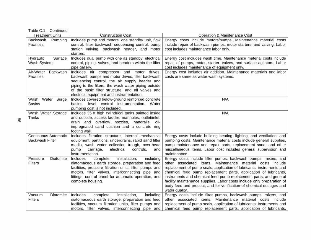
86


Backwash Pumping Facilities

Includes pump and motors, one standby unit, flow control, filter backwash sequencing control, pump station valving, backwash header, and motor starters.

Energy costs include motors/pumps. Maintenance material costs include repair of backwash pumps, motor starters, and valving. Labor cost includes maintenance labor only.

Hydraulic Surface Wash Systems

Includes dual pump with one as standby, electrical control, piping, valves, and headers within the filter pipe gallery.

Energy cost includes wash time. Maintenance material costs include repair of pumps, motor, starter, valves, and surface agitators. Labor cost includes maintenance of equipment only.

Air-Water Backwash Facilities

Includes air compressor and motor drives, backwash pumps and motor drives, filter backwash sequencing control, the air supply header and piping to the filters, the wash water piping outside of the basic filter structure, and all valves and electrical equipment and instrumentation.

Energy cost includes air addition. Maintenance materials and labor costs are same as water wash systems.

Wash Water Surge Basins

Includes covered below-ground reinforced concrete basins, level control instrumentation. Water pumping cost is not included.

N/A

Wash Water Storage Tanks

Includes 35 ft high cylindrical tanks painted inside and outside, access ladder, manholes, outlet/inlet, drain and overflow nozzles, handrails, oil-impregnated sand cushion and a concrete ring footing wall.

N/A

Continuous Automatic Backwash Filter

Includes filtration structure, internal mechanical equipment, partitions, underdrains, rapid sand filter media, wash water collection trough, over-head pump carriage, electrical controls, and instrumentation.

Energy costs include building heating, lighting, and ventilation, and pumping costs. Maintenance material costs include general supplies, pump maintenance and repair parts, replacement sand, and other miscellaneous items. Labor cost includes general supervision and maintenance.

Pressure Diatomite Filters

Includes complete installation, including diatomaceous earth storage, preparation and feed facilities, pressure filtration units, filter pumps and motors, filter valves, interconnecting pipe and fittings, control panel for automatic operation, and complete housing.

Energy costs include filter pumps, backwash pumps, mixers, and other associated items. Maintenance material costs include replacement of pump seals, application of lubricants, instruments and chemical feed pump replacement parts, application of lubricants, instruments and chemical feed pump replacement parts, and general facility maintenance supplies. Labor costs include only preparation of body feed and precoat, and for verification of chemical dosages and water quality.

Vacuum Diatomite Filters

Includes complete installation, including diatomaceous earth storage, preparation and feed facilities, vacuum filtration units, filter pumps and motors, filter valves, interconnecting pipe and

Energy costs include filter pumps, backwash pumps, mixers, and other associated items. Maintenance material costs include replacement of pump seals, application of lubricants, instruments and chemical feed pump replacement parts, application of lubricants,

87


fittings, control panel for automatic operation, and sitework and excavation around immediate vicinity.

instruments and chemical feed pump replacement parts, and general facility maintenance supplies. Labor costs include only preparation of body feed and precoat, and for verification of chemical dosages and water quality.

Pressure Filtration Plants

Includes complete filtration plant with vessels, cylinder operated butterfly valves, filter face piping and headers within the filter gallery, filter flow control and measurement instrumentation, headloss instrumentation, and a mass filter control panel. Housing is included.

Energy costs include process, and housing heating, lighting and ventilating. Maintenance materials include additional filter media, charts and ink for recorders, and miscellaneous repair items.

Taste and Odor Control Potassium Permanganate Feed Systems

Includes day tank, dual-head diaphragm pump, and metering pump (with one standby metering pump).

Energy costs for solution mixers and metering pumps, maintenance material costs as 3% of manufactured equipment cost, and labor costs for unloading drums of chemicals, preparation of solution, and routine operation of the solution metering pump were included.

Powdered Activated Carbon Feed Systems

Includes below ground uncovered concrete tanks, mixers, equipment for PAC feed, a diaphragm type metering pump (for less than 20 lb/hr feed rate) or a positive displacement-type pump (for more than 20 lb/hr feed rate), and an overhead rotodip volumetric feeder.

Energy costs include pump motors and continuous mixing. Maintenance material costs include oil for gearbox drives and minor repair of pumps, motors, and switching gear. Labor costs include unloading, inspection and routine maintenance, cleaning, gearbox oil change, and slurry pumps.

Disinfection Chlorine Storage and Feed

Cylinder Storage Use of 150 lb cylinders for feed rates up to 100 lb/day and ton cylinders for feed rates up to 2,000 lb/day. Maximum chlorinator capacity of 8,000 lb/day with one standby chlorinator per installation. Includes residual analyzers with flow-proportioning controls included for 1,000 lb/day and more, injector pumps, chlorinator room and cylinder storage room. Electrically operated, monorail trolley included for 100 lb/day and more.

Includes heating, lighting, and ventilation, electrical hoist (when cylinders are used), evaporators and injector pump. Cost of chlorine is not included. Labor requirements based on loading and unloading cylinders, time to connect and disconnect cylinders and time for routine daily checking (for cylinder storage). Labor requirements for on-site tank storage include time to unload bulk delivery truck or rail tanker. Labor requirements for rail car include time to move the rail car into place and to connect and disconnect cars from the feed system. Also includes checking and maintenance labor time for all systems.

On-site storage tank with rail delivery

Includes cost of turnout from the main line, 500 ft of on-site track, unloading platform.

Direct feed from Includes rail siding, chlorinator, evaporator, and

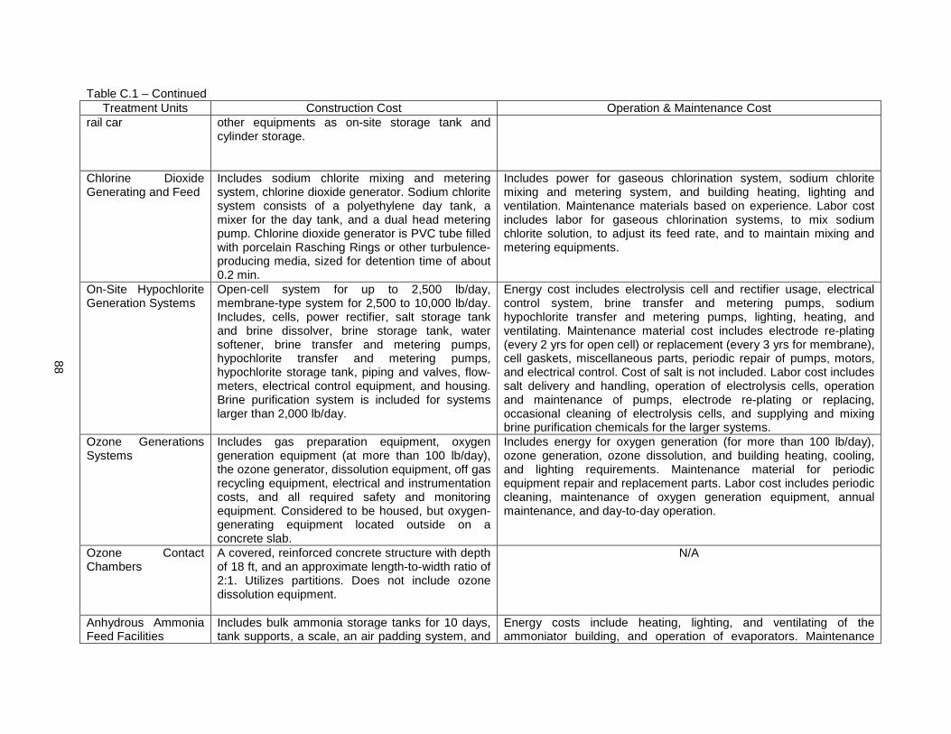
88


rail car other equipments as on-site storage tank and cylinder storage.

Chlorine Dioxide Generating and Feed

Includes sodium chlorite mixing and metering system, chlorine dioxide generator. Sodium chlorite system consists of a polyethylene day tank, a mixer for the day tank, and a dual head metering pump. Chlorine dioxide generator is PVC tube filled with porcelain Rasching Rings or other turbulence-producing media, sized for detention time of about 0.2 min.

Includes power for gaseous chlorination system, sodium chlorite mixing and metering system, and building heating, lighting and ventilation. Maintenance materials based on experience. Labor cost includes labor for gaseous chlorination systems, to mix sodium chlorite solution, to adjust its feed rate, and to maintain mixing and metering equipments.

On-Site Hypochlorite Generation Systems

Open-cell system for up to 2,500 lb/day, membrane-type system for 2,500 to 10,000 lb/day. Includes, cells, power rectifier, salt storage tank and brine dissolver, brine storage tank, water softener, brine transfer and metering pumps, hypochlorite transfer and metering pumps, hypochlorite storage tank, piping and valves, flow-meters, electrical control equipment, and housing. Brine purification system is included for systems larger than 2,000 lb/day.

Energy cost includes electrolysis cell and rectifier usage, electrical control system, brine transfer and metering pumps, sodium hypochlorite transfer and metering pumps, lighting, heating, and ventilating. Maintenance material cost includes electrode re-plating (every 2 yrs for open cell) or replacement (every 3 yrs for membrane), cell gaskets, miscellaneous parts, periodic repair of pumps, motors, and electrical control. Cost of salt is not included. Labor cost includes salt delivery and handling, operation of electrolysis cells, operation and maintenance of pumps, electrode re-plating or replacing, occasional cleaning of electrolysis cells, and supplying and mixing brine purification chemicals for the larger systems.

Ozone Generations Systems

Includes gas preparation equipment, oxygen generation equipment (at more than 100 lb/day), the ozone generator, dissolution equipment, off gas recycling equipment, electrical and instrumentation costs, and all required safety and monitoring equipment. Considered to be housed, but oxygen-generating equipment located outside on a concrete slab.

Includes energy for oxygen generation (for more than 100 lb/day), ozone generation, ozone dissolution, and building heating, cooling, and lighting requirements. Maintenance material for periodic equipment repair and replacement parts. Labor cost includes periodic cleaning, maintenance of oxygen generation equipment, annual maintenance, and day-to-day operation.

Ozone Contact Chambers

A covered, reinforced concrete structure with depth of 18 ft, and an approximate length-to-width ratio of 2:1. Utilizes partitions. Does not include ozone dissolution equipment.

N/A

Anhydrous Ammonia Feed Facilities

Includes bulk ammonia storage tanks for 10 days, tank supports, a scale, an air padding system, and

Energy costs include heating, lighting, and ventilating of the ammoniator building, and operation of evaporators. Maintenance

89


all required gauges and switches, an evaporator, an ammoniator, and flow-proportioning equipment.

material costs were based on experience. Labor costs include transfer of ammonia to storage tank, and day-to-day O&M.

Aqua Ammonia Feed Facilities

Includes one horizontal pressure vessel and its supports, piping and valves, and the metering pump.

Energy cost includes only operation of metering pump. Maintenance material costs include repair parts for metering pump, valve repairs, and painting of the storage tank. Labor costs include unloading, and O&M.

Reverse Osmosis Includes housing, structural steel and miscellaneous metalwork, tanks, piping, valves, pumps, reverse osmosis membrane elements and pressure vessels, flow meters, cartridge filters, acid and polyphosphate feed equipment, and cleaning equipment.

Energy costs include high-pressure feed-water pumps, other pumps and chemical feed equipment, and lighting, heating, and ventilating for housing. Maintenance material costs include membrane replacement, replacement of cartridge filters, membrane cleaning chemicals, and materials for periodic repair of pumps, motors, and electrical control equipment. Labor costs include cleaning and replacing membranes, replacing cartridge filters, maintaining pumps, determining and preparing proper dosages, maintaining chemical feed equipment, and monitoring performance.

Pressure Ion Exchange Softening

Includes contact vessels, resins, two open reinforced concrete salt storage/brining basins, pumping facilities, an eductor.

Energy costs include regenerant pumping, rinse pumping, backwash pumping, and building heating, lighting, and ventilation. Maintenance material costs include periodic repair and replacement of components (1% of construction cost), and resin replacement (13% of resin cost). Labor cost includes O&M or ion exchange vessels and pumping facilities.

Gravity Ion Exchange Softening

Pressure Ion Exchange Nitrate Removal

Includes two open reinforced concrete salt storage/brining basins, resins, pumping facilities, an eductor.

Energy costs include regenerant pumping, rinse pumping, backwash pumping, and building heating, lighting, and ventilation. Maintenance material costs include periodic repair and replacement of components (1% of construction cost), and resin replacement (25% of resin cost). Labor cost includes O&M or ion exchange vessels and pumping facilities.

Activated Alumina for Fluoride Removal

Includes contact vessels, 10 ft deep resins, a caustic dilution tank, sulfuric acid storage tank (for more than 70 mgd), metering pumps, and pumping facilities.

Energy costs include regenerant pumping, occasional backwash pumping, and building heating, lighting, and ventilation. Maintenance material costs include periodic repair and replacement of components (1% of construction cost), and activated alumina replacement (10% of activated alumina cost). Labor cost includes O&M or ion exchange vessels and pumping facilities.

Stability

90


Lime Feed Systems Hydrated lime for feed rates up to 50 lb/hr and quicklime at higher rates. Includes volumetric or gravimetric feeder, and dissolving tank with 5-min detention time for hydrated lime. Includes elevated hoppers for 30 day storage, lime slakers, dust collector, bin gate, flexible connection to the slaker, and standby slakers for quicklime.

Energy costs include feeder, slaker, and grit removal. Maintenance material costs were based on 3% of manufactured equipment costs. Lime cost is not included. Labor costs include unloading, O&M for lime feeder, slaker, and associated grit removal.

Re-carbonation Basin Includes reinforced concrete structure, complete with influent and effluent channels, foam suppression piping and sprayers, and handrails surrounding the basin.

N/A

Re-carbonation – Liquid CO2 as CO2 Source

Includes a storage tank with 10 days storage, two CO2 vaporizers and solution-type CO2 feeders (one of each is standby), an injector pump for the solution water, a stainless steel main header, diffuser pipes for the recarbonation basin, and an automatic control system.

Energy costs include injector pump and CO2 vaporizer. Maintenance material costs are based on experience from chlorine feed facilities. Labor cost includes only checking and adjustment of the feeder and vaporizer.

Re-carbonation – Submerged Burners as CO2 Source

Includes stainless steel submerged burner assembly, a pump, a centralized control panel, pipes and valves, automatic control.

Electricity cost includes pump. Natural gas cost is based on manufacturer’s recommendations. Maintenance material costs are based on 5% of manufactured equipment cost. Labor costs include oil change, cleaning air filter, and quarterly and annual maintenance.

Re-carbonation – Stack Gas as CO2 Source

Includes compressors, a compressed CO2 supply line, diffuser piping, and a pH-controlled feed system.

Energy cost includes compression of stack gas to 8 psi. Maintenance material costs include compressor repair parts, valve maintenance, and maintenance of electrical components. Labor cost includes maintenance of compressor and related accessories.

Clear Water Storage and Distribution Below-Ground Clearwell Storage

Includes reinforced concrete structures, instrumentation and control of clearwell water level, and instrumentation for turbidity and chlorine measurement and other quality control operations.

N/A

Ground-Level Clearwell Storage

Includes steel tanks, instrumentation and control of clearwell water level, and instrumentation for turbidity and chlorine measurement and other quality control operations.

N/A

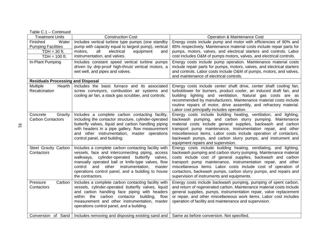
91


Finished Water Pumping Facilities

Includes vertical turbine type pumps (one standby pump with capacity equal to largest pump), vertical motors, all electrical equipment and instrumentation, and valves.

Energy costs include pump and motor with efficiencies of 90% and 85% respectively. Maintenance material costs include repair parts for pumps, motors, valves, and electrical starters and controls. Labor cost includes O&M of pumps motors, valves, and electrical controls.

TDH = 30 ft. TDH = 100 ft. In-Plant Pumping Includes constant speed vertical turbine pumps

driven by drip-proof high-thrust vertical motors, a wet well, and pipes and valves.

Energy costs include pump operation. Maintenance material costs include repair parts for pumps, motors, valves, and electrical starters and controls. Labor costs include O&M of pumps, motors, and valves, and maintenance of electrical controls.

Residuals Processing and Disposal Multiple Hearth Recalcination

Includes the basic furnace and its associated screw conveyors, combustion air systems and cooling air fan, a stack gas scrubber, and controls.

Energy costs include center shaft drive, center shaft cooling fan, turboblower for burners, product cooler, an induced draft fan, and building lighting and ventilation. Natural gas costs are as recommended by manufacturers. Maintenance material costs include routine repairs of motor, drive assembly, and refractory material. Labor cost principally includes operation.

Concrete Gravity Carbon Contactors

Includes a complete carbon contacting facility, including the contactor structure, cylinder-operated butterfly valves, liquid and carbon handling piping with headers in a pipe gallery, flow measurement and other instrumentation, master operations control panel, and building.

Energy costs include building heating, ventilation, and lighting, backwash pumping, and carbon slurry pumping. Maintenance material costs include general supplies, backwash and carbon transport pump maintenance, instrumentation repair, and other miscellaneous items. Labor costs include operation of contactors, backwash pumps, and carbon slurry pumps, and instrument and equipment repairs and supervision.

Steel Gravity Carbon Contactors

Includes a complete carbon contacting facility with vessels, face and interconnecting piping, access walkways, cylinder-operated butterfly valves, manually operated ball or knife-type valves, flow control and other instrumentation, master operations control panel, and a building to house the contractors.

Energy costs include building heating, ventilating, and lighting, backwash pumping and carbon slurry pumping. Maintenance material costs include cost of general supplies, backwash and carbon transport pump maintenance, instrumentation repair, and other miscellaneous items. Labor costs include cost of operation of contactors, backwash pumps, carbon slurry pumps, and repairs and supervision of instruments and equipments.

Pressure Carbon Contactors

Includes a complete carbon contacting facility with vessels, cylinder-operated butterfly valves, liquid and carbon handling face piping with headers within the carbon contactor building, flow measurement and other instrumentation, master operations control panel, and a building.

Energy costs include backwash pumping, pumping of spent carbon, and return of regenerated carbon. Maintenance material costs include general supplies, pumps, instrumentation repair, valve replacement or repair, and other miscellaneous work items. Labor cost includes operation of facility and maintenance and supervision.

Conversion of Sand Includes removing and disposing existing sand and Same as before conversion. Not specified.

92


Filter to Carbon Contactor (Carbon Bed Depth = 30”)

gravel, installing carbon collection troughs and related piping and valves outside of filter, installation of slurry pumps and related controls for transport of spent carbon, reactivated carbon storage tank, reactivated carbon eductors, and distribution piping.

Off-Site Regional Carbon Regeneration – Handling and Transportation

Includes elevated tanks (cylinder for less than 2000 ft3 or rectangular), stainless steel dewatering screens, and associated pipes and valves.

N/A

Multiple Hearth Granular Carbon Regeneration

Includes basic furnace, center shaft drive, furnace and cooling fans, spent carbon storage and dewatering equipment, auxiliary fuel system, exhaust scrubbing system, regenerated carbon handling system, quench tank, steam boiler, control panel, and instrumentation.

The costs are for operation of 100% of time. Electricity cost includes furnaces, building lighting and ventilation. Natural gas costs are as recommended by the manufacturers at 1000 BTU/scf. Maintenance material costs include maintenance and repair of electrical drive machinery, replacement of rabble arms, and damaged refractory materials. Labor cost principally includes operation of equipment.

Infrared Carbon Regeneration Furnace

Includes pre-manufactured furnace modules (drying, pyrolysis, and activation), spent carbon holding tank, dewatering feed screw, quench tank, after burner, wet scrubber, exhaust gas blower, all duck work, scrubber water piping and valves within process limits, process electrical equipment and controls, and prefabricated metal housing.

Energy cost includes operation of infrared heating units, cooling and exhaust blowers, scrubbing water system, and building lighting and ventilation. Maintenance material cost includes replacement cost of tungsten filament quartz heating units, small moving parts, and general equipment maintenance. Labor cost includes operation and maintenance of equipment.

Granular Carbon Regeneration – Fluid Bed Process

Includes spent and regenerated carbon storage, carbon dewatering system, fluid bed reactor, fluidizing air blower, quench tank, particulate scrubber, interconnecting piping and electrical equipment within process area limits, and controls and instrumentation. A 35 ft steel building is also included.

Electricity cost includes fluidizing air blower and other operation and maintenance requirements. Natural gas costs include heating. Maintenance material cost includes replacement parts for electrical drive machinery, damaged refractory materials, and other general maintenance items. Labor cost includes O&M of equipment.

Powdered Carbon Regeneration – Fluidized Bed Process

Includes fluidized bed reactor, cyclone and venture separators, heat exchangers, fluidizing air blower, carbon feed and removal equipment, process pumps and piping, and controls and instrumentation.

Electricity cost includes operating furnaces. Natural gas costs heating. Maintenance material costs include maintenance and repair of electrical drive and control machinery, replacement of FBF refractory materials, replacement of silica sand, and other general equipment maintenance items. Labor cost includes O&M of

93


equipment. Powdered Carbon Regeneration – Atomized Suspension Process

Includes manufactured equipment costs for basic reactor, spent carbon slurry storage tank, furnace feed pump, regenerated carbon recovery equipment, and exhaust scrubbing facilities – all furnished and installed, and installation labor cost.

Electricity cost includes process pumping and reactor air supply. Natural gas cost is for heating. Maintenance material costs include repair of electrically driven machinery, heating units, and routine maintenance of system. Labor cost includes operation of equipment.

Chemical Sludge Pumping – Unthickened Sludge

Includes variable speed horizontal centrifugal pump, one standby pump, pipes and valves, and housing above dry well. Entire dry well cost is not covered.

Energy cost includes pumping lime sludge with 65% efficiency. Maintenance material costs include periodic repair of the pumps, motors, and electrical control units. Labor cost includes periodic checking of pumps and motors, and periodic maintenance.

Chemical Sludge Pumping – Thickened Sludge

Includes progressive cavity pump and motors, required pipes and valves, electrical equipment and instrumentation, and housing.

Energy cost includes pumping thickened lime mud. Maintenance material costs include periodic repair of the pumps, motors, and electrical control units. Labor cost includes periodic checking of pumps and motors, and periodic maintenance.

Gravity Sludge Thickeners

Includes cost of thickener mechanism and its installation, and reinforced concrete structure with 12 ft sidewall.

Energy cost includes average cost for driving thickener mechanism for lime, alum, and ferric sludge. Maintenance material and labor costs include repair and normal maintenance of thickener drive mechanism and weirs.

Vacuum Filters Includes vacuum drum filter, vacuum and filtrate pump assemblies, precast pump and storage tanks, belt, conveyor, interconnecting piping, electrical controls and housing.

Electricity costs include drum drive, discharge roller, vacuum and filtrate pumps, precoat pump, tank agitators, and belt conveyor. Maintenance material and labor costs include estimated annual costs for filter operation and maintenance, and for replacement parts.

Sludge Dewatering Lagoons

Includes unlined lagoons. Land cost is not included.

Includes sludge removal from the lagoon.

Filter Press Includes the filter press, feed pumps (including one standby), a lime storage bin and feeders, a sludge conditioning and mixing tank, an acid wash system, and housing.

Energy costs include operation of feed pump, open-close mechanism and tray mover. Maintenance material and labor costs include annual costs estimated from manufacturers’ experience and data from several operating installations.

Decanter Centrifuges Includes decanter centrifuge and provisions for preparation, storage, and application of polymers.

Energy costs include main drive unit, back drive unit, and polymer preparation and feed equipment. Maintenance material costs include annual cost for replacement parts and miscellaneous components, and for general maintenance. Labor costs include start-up and adjustment, polymer preparation, and occasional maintenance involving machine and motor lubrication.

94


Basket Centrifuges Includes basket centrifuge and equipments for preparation, storage, and application of polymers.

Energy costs include machine acceleration, sludge feeding, skimming, decelerating, and sludge plowing. Energy costs also include polymer preparation and feed equipment. Maintenance material costs include annual cost for maintenance, replacement parts, lubrication, and other consumable items. Labor costs include start-up and adjustment, polymer preparation, and required maintenance.

Sand Drying Beds Includes uncovered and unlined sand drying beds, sludge distribution piping, 9 inch of sand overlying 9 inch of gravel media, 2 ft concrete dividers between beds, and underdrain system. Land cost is not included.

Energy cost includes front-end loader. Maintenance material cost includes replacement of sand lost during bed cleaning. Labor costs include sludge removal and bed preparation.

Belt Filter Press Includes belt press unit, wash pump, conditioning tank, feed pump, polymer storage tank and pump, belt conveyor, and electrical control panel.

Energy costs include belt drive unit, belt wash pump, conditioning tank, feed pump, polymer pump and tanks, belt conveyor, and electrical control panel. Maintenance material and labor costs are based on equipment manufacturers’ data.

Management Administrative, Laboratory and Maintenance Building

Based on building area review of over dozen of treatment facilities.

Includes O&M costs related to administrative, laboratory, and maintenance functions. Energy cost is based on building area requirement. Maintenance material costs are not directly assignable to specific plant components and include O&M of administrative facilities such as office supplies, communications, dues, subscriptions, office equipment repairs, travel expenses, training course expense, and custodial supplies. Labor costs include only administration and management of plant like superintendent, assistant superintendent, plant chemist, bacteriologist, clerk, and maintenance supervisor.

95

APPENDIX D

LIST OF ABBREVIATIONS

96

BCI Building Cost INdex

BLS Bureau of Labor Statistics

BOD5 5-day Biochemical Oxygen Demand

CC Construction Cost

CCI Construction Cost Index

COD Chemical Oxygen Demand

CRF Capital Recovery Factor

DCS Distributed Control System

ED Electrodialysis

ENR Engineering News-Record

ES Effective Size

GAC Granular Activated Carbon

LI Langelier Saturation Index

MF Microfiltration

NF Nanofiltration

O&M Operation and Maintenance

O&MC Operation and Maintenance Cost

PAC Powdered Activated Carbon

PW Present Worth

RO Reverse Osmosis

SCADA Supervisory Control and Data Acquisition

THM Trihalomethane

ThOD Theoritical Oxygen Demand

TOC Total Organic Compound

TOD Total Oxygen Demand

TOX Total Organic Halogen

T&O Taste and Odor

UF Ultrafiltration

97

UO Unit Operation

UP Unit Process

USEPA United States Environmental Protection Agency

UV Ultraviolet

VOC Volatile Organic Compound

98

REFERENCES

Amirtharajah, A., and O'Melia, C. R. (1990). "Coagulation Processes: Destabilization, Mixing, and Flocculation." Water Quality and Treatment: A handbook of Community Water Supplies - Fourth Edition, American Water Works Association, ed., McGraw-Hill, Inc., New York, 269-365.

ASCE, and AWWA. (1990). Water Treatment Plant Design, Second Edition. McGraw-Hill, Inc., New York.

Bureau of Labor Statistics. (2009). "Producer Price Index Commodity Data." http://data.bls.gov/PDQ/outside.jsp?survey=wp (10/22, 2009).

Bureau of Labor Statistics. (1992a). "Producer Price and Price Indexes: Data of April 1992." US Department of Labor, Washington, D.C.

Bureau of Labor Statistics. (1992b). "Producer Price Index Historical." US Department of Labor, Washington, D.C.

Bureau of Labor Statistics. "Producer Prices and Price Indexes: Data for 1978." Rep. No. 1978, US Department of Labor, Washington, D.C.

Cleasby, J. L. (1990). "Filtration." Water Quality and Treatment: A Handbook of Community Water Supplies, Forth Edition, American Water Works Association, ed., McGraw-Hill, Inc, New York, 455-560.

Clifford, D. A. (1990). "Ion Exchange and Inorganic Adsorption." Water Quality and Treatment: A Handbook of Community Water Supplies, Forth Edition, American Water Works Association, ed., McGraw-Hill, Inc., New York, 561-639.

Conlin, W. J. (1990). "Membrane Processes." Water Quality and Treatment: A Handbook of Community Water Supplies, Forth Edition, American Water Works Association, ed., McGraw-Hill, Inc., New York, 709-746.

Cornwell, D. A. (1990). "Air Stripping and Aeration." Water Quality and Treatment - A Handbook of Community Water Supplies, Forth Edition, American Water Works Association, ed., McGraw-Hill, Inc., New York, 229-268.

Doe, P. W. (1990). "Water Treatment Plant Waste Management." Water Quality and Treatment: A Handbook of Community Water Supplies, Forth Edition, American Water Works Association, ed., McGraw-Hill, Inc., McGraw-Hill, Inc., 955-996.

Elarde, J. R., and Bergman, R. A. (2001). "The Cost of Membrane Filtration for Municipal Water Supplies." AWWA Membrane Technology Conference Proceedings, American Water Works Association, Denver, Colorado, .

Energy Information Administration. (2010). "Average Retail Price of Electricity to Ultimate Customers by End-Use Sector." http://www.eia.doe.gov/cneaf/electricity/epm/table5_6_a.html (2/19, 2010).

99

Energy Information Administration. (2010). "Natural Gas Monthly." Rep. No. DOE/EIA‐0130(2010/01), Energy Information Administration, Wahington, DC.

Energy Information Administration. (2010). "Weekly Retail On-Highway Diesel Prices." http://tonto.eia.doe.gov/oog/info/wohdp/diesel.asp (2/19, 2010).

Engineering News-Record. (2010). "Construction Economics." ENR: Engineering News-Record, 264(4), 18-19.

Engineering News-Record. (2009). "Construction Economics." ENR, 263(9), 108-111.

Engineering News-Record. (1978). "Construction Scoreboard." ENR, 201(16), 93.

Glaze, W. H. (1990). "Chemical Oxidation." A Handbook of Community Water Supplies, Forth Edition, American Water Works Association, ed., McGraw-Hill, Inc., New York, 747-779.

Gregory, R., and Zabel, T. F. (1990). "Sedimentation and Flotation." Water Quality and Treatment: A Handbook of Community Water Supplies, Forth Edition, American Water Works Association, ed., McGraw-Hill, Inc., New York, 367-453.

Grogan, T. (2009). "How To Use ENR's Cost Indexes." ENR: Engineering News-Record, 262(9), 37-38.

Grogan, T. (1994). "Cost History: Indexes Hit by High Lumber Prices." ENR: Engineering News-Record, 232(13), 48.

Gumerman, R. C., Culp, R. L., and Hansen, S. P. (1979). "Estimating Water Treatment Costs." Rep. No. EPA-600/2-79-162a-d, Municipal Environmental Research Laboratory, Office of Research and Development, U.S. Environmental Protection Agency, Cincinati, Ohio 45268.

Haas, C. N. (1990). "Disinfection." Water Quality and Treatment: A Handbook of Community Water Supplies, Forth Edition, American Water Works Association, ed., McGraw-Hill, Inc., New York, 977-932.

Holm, L., Schaufelberger, J. E., Griffin, D., and Cole, T. (2005). Construction Cost Estimating: Process and Practices. Pearson Education, Inc., Upper Saddle River, New Jersey.

Kawamura, S. (2000). Integrated Design and Operation of Water Treatment Facilities. John Wiley & Sons, Inc., New York.

Kleinbaum, G. G., Lawrence, L. K., Muller, K. E., and Nizam, A. (1998). Applied Regression Analysis and Other Multivariable Methods, Third Edition. Brooks/Cole Publishing Company, Pacific Grove, California.

Qasim, S. R., Lim, S. W. (., Motley, E. M., and Heung, K. G. (1992). "Estimating costs for treatment plant construction." J.Am.Water Works Assoc., 84(8), 56-62.

Qasim, S. R., Motley, E. M., and Zhu, G. (2000). Water Works Engineering: Planning, Design & Operation. Prentice-Hall, Inc., Upper Saddle River, NJ.

Remer, D. S., Lin, S., Yu, N., and Hsin, K. (2008). "An update on cost and scale-up factors, international inflation indexes and location factors." Int J Prod Econ, 114(1), 333-346.

100

Snoeyink, V. L. (1990). "Adsorption of Organic Compounds." Water Quality and Treatment: A Handbook of Community Water Supplies, Forth Edition, American Water Works Association, ed., McGraw-Hill, Inc., McGraw-Hill, Inc., 781-875.

Vernick, A. S., and Walker, E. C. (1981). Handbook of Water Treatment Processes. Marcel Dekker, Inc., New York.

101

BIOGRAPHICAL INFORMATION

Jwala Raj Sharma completed his Bachelor’s Degree in Civil Engineering from Institute of

Engineering, Tribhuvan University in Kathmandu, Nepal. He started MS in Civil Engineering at the

University of Texas at Arlington in Fall 2008. During his time at the UTA, he contributed in various

researched. He aspires to continue with more researches.

development of a preliminary cost estimation

Documents