development of a novel lc-ms/ms method …development of a novel lc-ms/ms method for the detection...

DEVELOPMENT OF A NOVEL LC-MS/MS METHOD FOR THE DETECTION OF ADULTERATION OF SOUTH

AFRICAN SAUVIGNON BLANC WINES WITH 3-ALKYL-2-METHOXYPYRAZINES.

P. Alberts

Thesis presented in partial fulfillment of the requirements for the degree of

Master of Science (Chemistry)

at

Stellenbosch University

Dr. A. J. de Villiers (supervisor) Stellenbosch

Dr. M. A. Stander (co-supervisor) March 2008

i

Declaration

I, the undersigned, hereby declare that the work contained in this thesis is my

own original work and that I have not previously in its entirety or in part submitted

it at any university for a degree.

Signature:__________________________

Date:______________________________

Copyright © 2008 Stellenbosch University

All rights reserved

ii

Summary

A method for the detection of adulteration of South African Sauvignon blanc

wines, by enrichment with foreign sources of 3-alkyl-2-methoxypyrazenes, is

described. The levels of three 3-alkyl-2-methoxypyrazenes (3-isobutyl-, 3-

isopropyl- and 3-sec-butyl-2-methoxypyrazine) in South African Sauvignon blanc

wines were measured with liquid chromatography-mass spectrometry. Sample

preparation involved clean-up and pre-concentration by distillation followed by

solvent extraction of the distillate with dichloromethane. Extracts were acidified

and concentrated by evaporation and finally reconstituted to a fixed volume to

affect quantitative pre-concentration of the samples. Sample extracts were

separated with reversed phase liquid chromatography utilizing a phenyl-hexyl

separation column. Residues were measured with liquid chromatography-mass

spectrometry utilizing a tandem quadrupole mass spectrometric detector

operated in multiple reaction monitoring mode for optimal trace level quantitation.

Atmospheric pressure chemical ionization was utilized as electrospray ionization

was found to suffer from quenching effects attributed to the sample matrix.

Qualitative information was obtained from the relevant molecular ions as well as

two secondary ion transitions (and one ion ratio) in each case. Recoveries

obtained by the extraction procedure were better than 90% with coefficient of

variance of better than 10% at concentrations from 1 to 100 ng/L. The limit of

detection of the method was 0.03 ng/L and the limit of quantification 0.10 ng/L for

the three analytes measured. The described LC-MS method is more sensitive for

the determination of 3-alkyl-2-methoxypyrazines in wine than GC methods

reported for the same purpose.

From the experimental data, a set of parameters were established to discriminate

adulterated South African Sauvignon blanc wines. It was demonstrated that the

3-isobutyl-2-methoxypyrazine concentration, despite showing considerable

variance, was confined to a relatively narrow range spanning approximately two

orders of magnitude (0.20 to 22 ng/L). A clear indication of possible maximum

iii

values for this compound in South African Sauvignon blanc wines was obtained

from the analysis of a large number of samples (577), spanning most relevant

wine producing regions and representing vintages 2003 to 2006. It was also

demonstrated that South African Sauvignon blanc wines contain the major 3-

alkyl-2-methoxypyrazenes in reasonably distinct relative amounts and that the

said ratios of abundance may be used to elucidate authenticity. The expected

effect of adulteration with green pepper extracts or some synthetic preparations

on the 3-isobutyl-2-methoxypyrazine concentration as well as the relative

abundances were also determined by characterizing the corresponding profiles in

green peppers and some synthetic flavor preparations. Two adulterated samples

in the dataset were identified by both outlined criteria. A limited number of wines

of other cultivars were also analyzed. The results represent the most complete

and accurate data on the 3-alkyl-2-methoxypyrazine content of South African

Sauvignon blanc wines to date.

A publication covering the work presented in this thesis is currently in

preparation.

iv

Opsomming

`n Metode word beskryf vir die opsporing van vervalsing van Suid-Afrikaanse

Sauvignon blanc wyn met wynvreemde bronne van 3-alkiel-2-metoksiepirasiene

om die soetrissiegeur daarvan te bevorder. Die vlakke van drie 3-alkiel-2-

metoksiepirasiene (3-isopropiel-, 3-isobutiel- en 3-sek-butiel-2-metoksiepirasien)

is bepaal deur middel van vloeistofchromatografie-massaspektrometrie.

Monstervoorbereiding behels distillasie gevolg deur vloeistofekstraksie met

dichlorometaan. Ekstrakte is aangesuur en die oplosmiddel is afgedamp waarna

dit opgemaak is tot ’n bekende volume. Die ekstrakte is met feniel-heksiel

gebaseerde omgekeerdefase vloeistofchromatografie geskei en die vlakke van

drie 3-alkiel-2-metoksiepirasiene in Suid-Afrikaanse Sauvignon blanc wyn is met

behulp van massaspektrometrie gemeet. Die massaspektrometer is in multi-

reaksie moniteringsmodus gebruik om optimale spoor-vlak kwantifisering te

bewerkstellig terwyl kwalitatiewe inligting uit ioon-oorgange en verhoudings

verkry is. Positiewelading atmosferiesedruk chemiese ionisasie is gebruik nadat

bevind is dat elektrosproei-ionisasie deur die matriks onderdruk is. Die

herwinning met die metode behaal, is beter as 90% met koeffisiënt van variasie

van beter as 10% by konsentrasies tussen 1 en 100 ng/L. Die deteksielimiet was

0.03 ng/L en kwantifiseringslimiet 0.10 ng/L, vir al drie analiete. Die metode bied

beter sensitiwiteit vir die bepaling van 3-alkiel-2-metoksiepirasiene in wyn as

gaschromatografiese metodes wat vir dieselfde doel aangewend is.

Die eksperimentele data is gebruik om parameters vas te stel waarvolgens

vervalsde wyn onderskei kon word. Dit is gedemonstreer dat die 3-isobutiel-2-

metoksiepirasienkonsentrasie, ten spyte van beduidende variasie, beperk is tot ’n

redelike nou konsentrasiegebied. Die vlakke het gevarieer oor twee ordegroottes,

tussen ongeveer 0.20 en 22 ng/L. Hierdie inligting het egter ’n duidelike

aanduiding van moontlike perke wat vir die komponent in Suid-Afrikaanse

Sauvignon blanc wyn verwag kan word, gelewer aangesien ’n statisties

beduidende aantal monsters ontleed is (577) en die relevante produserende

v

areas goed verteenwoordig is. Oesjare tussen 2003 en 2006 is ook goed

verteenwoordig in die studie. Verder is dit ook duidelik dat Suid-Afrikaanse

Sauvignon blanc wyn die drie vernaamste 3-alkiel-2-metoksiepirasiene in

redelike konstante relatiewe hoeveelhede bevat. Die relatiewe verhouding van

die genoemde stowwe is ook in soetrissie en sintetiese middels bepaal en

aangesien die verhouding daarvan in wyn beduidend verskil het van die in

soetrissie en sintetiese middels, kon vervalsing ook hieruit bepaal word. Die

verwagte invloed van vervalsing met soetrissie en sintetiese middels op die

relatiewe hoeveelhede in wyn kon gevolglik bepaal word. Hierdie twee faktore

kon dus gebruik word om vervalsing van Suid-Afrikaanse Sauvignon blanc wyn

met soetrissie ekstrakte en sintetiese middels te bepaal. Twee vervalsde wyne is

met beide strategieë gëidentifiseer. `n Beperkte aantal wyne van ander kultivars

is ook met die metode ontleed. Die resultate wat in hierdie studie verkry is,

verteenwoordig die volledigste inligting betreffende die 3-alkiel-2-

metoksiepirasiene in Suid-Afrikaanse Sauvignon blanc wyn.

vi

Acknowledgements

I would like to express my gratitude to the following persons and institutions:

• The supervisors for the project, Drs. A.J. de Villiers and M.A. Stander.

• Professor S.O. Paul for help with statistical analysis of the data.

• The South African National Department of Agriculture, in particular Mr. A.

Smith for facilitating the project.

• The Wine and Spirit Board of South Africa, in particular Mr. H van der

Merwe, for providing samples of Sauvignon blanc wine.

• For their kind assistance with method development and sample

preparation, my colleagues A. le Roux, W. Ndaba, J. Waries and M.

Maarman.

• J. Ebersohn, representative for Waters Micromass, for efficient and

professional support.

vii

Abbreviations

APCI

atmospheric pressure chemical ionization

S/N SBMP

signal-to-noise ratio 3-sec-butyl-2-methoxypyrazine

cGC capillary gas chromatography SBSE stir bar sorptive extraction CI confidence interval SDB styrene-divinylbenzene CL confidence limits SIM single-ion monitoring DAD diode array detector SPE solid phase extraction DC direct current SPME solid phase microextraction DCM dichloromethane Stdev Standard deviation DVB divinylbenzene TIC total ion chromatogram EI electron-impact ionization TOF time-of-flight EMP 3-ethyl-2-methoxypyrazine UV ultraviolet ESI electrospray ionization UV-Vis ultraviolet visible EU European Union v / v volume-per-volume GC gas chromatography GC-MS

gas chromatography mass spectrometry

HPLC

high-performance liquid chromatography

IBMP 3-isobutyl-2-methoxypyrazine ID internal diameter IPEP 3-isopropyl-2-ethoxypyrazine IPMP 3-isopropyl-2-methoxypyrazine LC liquid chromatography LC-MS

liquid chromatography-mass spectrometry

m/v mass per volume m/z mass to charge ratio MDL minimum detection limit MMP 3-methyl-2-methoxypyrazine MQL minimum quantification limit MRM multiple reaction monitoring MS mass spectrometer ND not detected NPD nitrogen-phosphorus detector NQ not quantified PC principal component PCA principal component analysis PDMS polydimethylsiloxane PEG polyethylene glycol PSDVB polystyrene divinylbenzene Q quadrupole analyzer QTOF quadrupole time-of-flight RF radio frequency RP-LC

reversed phase liquid chromatography

RSD relative standard deviation

Table of contents

Declaration i

Summary ii

Opsomming iv

Acknowledgements vi

Abbreviations vii

CHAPTER 1 1 Introduction 1

1.1. Historical perspective on wine and adulteration 1

1.2. Sauvignon blanc wine 4

1.3. Origin, chemical properties and flavor characteristics of

methoxy-pyrazines 6

1.4. Analytical methodologies for the analysis of methoxypyrazines in wine 10

1.5. Detection of adulteration: Characterization of the profile of

relative abundance of the major 3-alkyl-2-methoxypyrazines in

Sauvignon blanc wine 13

1.6. Proposed methodology for characterizing the profile of

3-alkyl-2-methoxypyrazines in South African Sauvignon blanc wine 16

CHAPTER 2 23 Analytical techniques 23

2.1. Introduction 23

2.2. General description of chromatography 23

2.2.1. Migration rates of solutes in chromatographic separations 25

2.2.2. Band broadening in chromatography 27

2.2.3. Optimization of chromatographic resolution 31

2.2.4. Differences between liquid chromatography and

gas chromatography 32

2.3. High performance liquid chromatography 33

2.3.1. The HPLC column 33

2.3.2. Column efficiency in HPLC 34

2.3.3. Modes of separation in liquid chromatography 35

2.3.4. HPLC instrumentation 39

2.3.5. Mobile phase treatment system 40

2.3.6. Solvent delivery system 41

2.3.7. Sample injection systems 43

2.3.8. Column thermostat 44

2.3.9. Detectors 45

2.4. Gas chromatography 58

2.4.1. Gas chromatographic columns 58

2.4.2. Carrier gases 60

2.4.3. Sample injection systems 60

2.4.4. Derivativization 63

2.4.5. Column oven 63

2.4.6. Detectors 63

CHAPTER 3 69 Development and optimization of a sample preparation procedure for the

liquid chromatographic analysis of trace levels of 3-alkyl-2-methoxypyrazines

in wine 69

3.1. Introduction 69

3.2. Experimental 72

3.2.1. Materials 72

3.2.2. Liquid chromatographic methods and instrumentation 74

3.3. Results and discussion 75

3.3.1. HPLC method performance 75

3.3.2. Development and optimization of a solvent extraction

procedure 78

3.3.3. Evaluation of distillation as sample treatment for the analysis

of methoxypyrazines in wine 84

3.3.4. Evaluation of solid phase extraction for the isolation and

pre-concentration of 3-isobutyl-2-methoxypyrazine from wine 93

3.3.5. Evaluation of stir bar sportive extraction (SBSE) for the

isolation and pre-concentration of IBMP from wine 107

3.4. Conclusions 109

CHAPTER 4 115 Development of an optimized liquid chromatography - mass spectrometric method for

trace level quantitation of selected 3-alkyl-2-methoxypyrazines 115

4.1. Introduction and objectives 115

4.2. Experimental 116

4.2.1. Materials 116

4.2.2. Instrumentation 116


4.3.1. Initial selection of chromatographic separation mode 118

4.3.2. Determination of the optimal flow rate in the chromatographic separation

utilizing 4.6 mm diameter columns 122

4.3.3. Determination of optimal ionization parameters for the

LC-MS analysis of methoxypyrazines 123

4.3.4. Optimization of positive mode electrospray ionization

parameters 125

4.3.5. Reversed phase separation of methoxypyrazines using

optimized electrospray ionization conditions 137

4.3.6. Method specificity utilizing isocratic reversed phase

separation and electrospray ionization 143

4.3.7. Atmospheric pressure chemical ionization 143

4.3.8. Efficiency of atmospheric pressure chemical ionization in

various elution systems utilized in reversed phase separations 144

4.3.9. Effect of the orientation of the APCI probe on ionization

efficiency 146

4.3.10. Effect of mobile phase flow-rate on ionization efficiency 148

4.3.11. Optimisation of APCI source parameters 149

4.3.12. Optimisation of instrument tuning parameters for MS-MS operation 152

4.3.13. Method specificity utilizing separation on a C18 column and atmospheric

pressure chemical ionization 154

4.3.14. LC-APCI-MS analysis of methoxypyrazines in wine 160


CHAPTER 5 168 Validation of the optimized RP-LC-APCI-MS method for the analysis of

3-alkyl-2-methoxypyrazines in wine 168


5.2. Materials and methods 168

5.2.1. Chemicals and samples 168

5.2.2. Sample preparation 169

5.2.3. Chromatographic details 170


5.3.1. Minimum method criteria 170

5.3.2. Determination of the linear working range 172

5.3.3. Limits of detection and quantitation 177

5.3.4. Method specificity 179

5.3.5. Method accuracy 180

5.3.6. Method precision 181

5.3.7. Uncertainty of measurements and reporting of results 181

5.3.8. System stability 182


CHAPTER 6 186 The contents of some 3-alkyl-2-methoxypyrazines in South African

Sauvignon blanc wine and detection of adulteration 186


6.2. Materials and methods 187

6.2.1. Samples 187

6.2.2. Sample preparation 188

6.2.3. Chromatographic details 189

6.2.4. Statistical methods 190


6.3.1. Sauvignon blanc wines 190

6.3.2. 3-Alkyl-2-methoxypyrazine content of other cultivars 208

6.3.3. Multivariate analysis of the 3-alkyl-2-methoxypyrazine data 209


CHAPTER 7 228 Summary and final concluding remarks 228

APPENDIX 1: MASS SPECTRA OF COMPONENTS OF INTEREST 234

APPENDIX 2: QUANTITATIVE DATA FOR WINES ANALYZED

IN THE STUDY 237

APPENDIX 3: PICTURES 255

1

CHAPTER 1

Introduction

1.1. Historical perspective on wine and adulteration

Wine may have an archeological origin dating back more than 7.5 thousand

years, with the earliest suspected wine residues dating from the early to mid-

fifth millennium B.C. Clear evidence of intentional winemaking first appears in

representations of wine presses that date back to the reign of Udimu in Egypt,

some 5000 years ago. The development of wine-making and the

domestication of the wine grape, Vitis vinifera, are thought to have occurred in

southern Caucasia, an area that includes parts of present-day north-western

Turkey, northern Iraq, Azerbaijan and Georgia. Domestication may also have

occurred independently in Spain.

The evolution of wine-making from an infrequent occurrence to a routine

agricultural event may have followed the development of a settled agricultural

lifestyle. At the same time, beneficial properties such as low mineral and water

requirements as well as excellent regenerative powers and woody structure,

which have permitted the grapevine to withstand considerable winterkill while

producing acceptable yields in cool climates, favored its cultivation and the

spread of viticulture. For ancient humans, the result of grape fermentation was

the transformation of a perishable, periodically available fruit into a relatively

stable beverage with novel and potentially intoxicating properties. Wine also

developed an association with religious rites with much symbolic value.

From Caucasia, grape growing and wine making spread into Palestine, Syria,

Egypt and Mesopotamia and from this base wine consumption and its socio-

religious connections reached the Mediterranean. In more recent times,

European exploration and colonization have spread grapevine cultivation into

most of the temperate climatic regions of the globe. Wines began to take on

2

their modern expression in the 17th century when the use of sulfur in barrel

treatment are thought to have become widespread, thus greatly increasing the

likelihood of producing better-quality wines and extending their aging

potential. The utilization of glass bottles and cork as a closure in the 17th

century provided conditions favorable for the production of modern wine. With

the discovery by Pasteur around 1860 of the central importance of yeasts and

bacteria to fermentation, the chain of events was set in motion that has

produced the incredible range of wines that typifies modern commerce. From

these humble origins, grape production has developed into the world’s most

important fresh fruit crop. Worldwide grape production in 1992 exceeded that

for oranges, bananas or apples. The area planted under grapevines in 1990

was estimated at about 8.7 million hectares of which approximately 71% of

the yield was fermented into wine.1

South Africa has a long history of winemaking, dating back to 1655, when Jan

van Riebeeck planted the first vines in the Cape. In 1659 the first wine was

made from these plantings. In the late 18th and early 19th centuries the Cape

wine industry became famous for Constantia, a sweet, fortified wine that was

much sought-after in the royal courts of Europe and was venerated by writers

of that time. Napoleon Bonaparte reputedly requested a bottle of Constantia

on his deathbed. The specialization in fortified wine production is still evident

in the South African wine industry today as about half of its capacity is

dedicated to fortified wine and brandy. In modern times the South African wine

industry started to blossom after the Second World War, with the perfection of

cold fermentation techniques for white wines. Since the recent transition to a

democracy, South African wine exports proliferated, mainly to the United

Kingdom, the Netherlands and other European destinations. The explosive

growth in wine exports from South Africa are demonstrated by the fact that it

increased from 855 000 cases in 1990 to 15.4 million cases in 2000, an

incredible 1 700 percent increase. At the present day, the South African

industry is changing from predominantly white to red wines, as is reflected by

the fact that 75% of new plantings are red varieties, particularly Cabernet

Sauvignon and Shiraz. This transition reflects the fact that the climate in South

Africa is more conducive to Bordeaux and Rhône-style wines.1,2 South Africa

3

also posses a red variety of own, Pinotage, which is a cross between Pinot

Noir and Cinsaut.3

The thorny issue of defining exactly what is wine has historically been

contentious and remains difficult to answer to this date. The variability and

value of wine have traditionally made it a target for unscrupulous operators

and the wine trade has been beset with adulteration and fraud throughout its

history. The long human chain stretching from grower to consumer affords

many opportunities for illegal practices. As early as the first century A.D.,

Pliny the Elder bemoaned the fact that not even the nobility was exempt from

falling victim to fraudulent practices in the wine trade of his time.

It is also important to recognize that the law viewed the same procedures

differently through the ages, sometimes condoning and sometimes

condemning identical practices. The simplest and most obvious form of

adulteration is the addition of water to the product to increase the volume.

Dilution of wine with water was however an accepted practice in ancient

Greece. Another obvious means of increasing volumes of wine is to blend it

with spirits or other inferior wines. This practice was common among

Bordeaux merchants of the 18th century who blended fine clarets destined for

the English market with rough wines imported from Spain, the Rhône or the

Midi, to increase profits. Systematization by the Portuguese government of the

practice of adding Brandy to wine eventually led to the production of Port as it

is known today.4 One particularly controversial method of altering the nature

of wine is the addition of sugar during fermentation to increase the eventual

alcoholic strength, a practice also known as Chaptalization.

One of the most common forms of fraud does not involve the addition of any

substance to the product, but merely the label. An early example of fraud

involving the region of origin of wine from Roman times, involved passing

ordinary wines off as valuable Falernian, the most highly prized Italian wine

from that period. Today, controlled appellations, a method based on the

French system, are widely used for labeling wine and designating quality and

geographical delimitation. The adoption of controlled appellation systems as

4

well as regulations and legislation served to create the legal apparatus to

combat fraud and adulteration so that although once rife, it is considerably

rarer in the wine trade of today.4,5

1.2. Sauvignon blanc wine

Sauvignon blanc is the vine variety solely responsible for some of the world’s

most popular and most distinctive dry white wines with the best examples of

the cultivar produced in France, particularly those from Sancerre and Pouilly-

Fumé.5 Sauvignon blanc is also one of the most important white wine cultivars

in South Africa.6 In 2004, 6944 ha of Sauvignon blanc were cultivated in South

Africa, which represented 12.8% of white wine varieties and 6.9% of total wine

variety plantings.7 Sauvignon blanc’s most identifiable characteristic is its

piercing, instantly recognizable aroma, described as various nuances of

green, grassy, herbaceous, green pepper, asparagus and gooseberry.5,6,8

Variously substituted 3-alkyl-2-methoxypyrazines are known to contribute to

the distinctive vegetal and herbaceous character associated with wine of this

cultivar.6,8,9

Sauvignon blanc wine is extremely sensitive to climatic, viticultural and

production factors, partly due to the temperature and light-sensitivity of the 3-

alkyl-2-methoxypyrazines.6,9,10 In South Africa, Sauvignon blanc grapes ripen

early in mid-season. At optimum maturity the average sugars are 21 to 24°

Balling with a total titratable acidity of 6 to 7 g/L.11 In the grapes, the

concentration of 3-alkyl-2-methoxypyrazines decrease as a result of solar

exposure during ripening.9,10 Consequently, in unsuitable, hotter climates,

high concentrations at harvest is usually associated with a lack of ripeness

and may have a negative impact on wine aroma quality.6 Sauvignon blanc

wine is therefore better adapted to cooler climates as higher overall aroma

concentrations are observed in wines produced in the cooler regions.6 The

South African climate is therefore generally not conducive to the production of

Sauvignon blanc wine possessing the desired and characteristic vegetal and

herbaceous character associated with products from France and New

5

Zealand. In South Africa, Sauvignon blanc wines with a pungent and precise

varietal character are only produced in cool localities and by applying specific

canopy management and enological practices.9,12 A number of outstanding

Sauvignon blanc wines have nevertheless been produced in South Africa,

contrary to the climatological suitability of the region and to the surprise of

eminent wine-writers.12

Flavor and aroma not only contributes to the varietal and regional

distinctiveness of wine, but also has a dramatic influence on the price of the

product. Adulteration of some South African Sauvignon blanc wines by

enrichment with foreign sources of 3-alkyl-2-methoxypyrazines have recently

been confirmed.13 It is suspected that the alkylmethoxypyrazine levels in the

adulterated wines were enriched with extracts obtained from green peppers.

The possibility that synthetic alkylmethoxypyrazine preparations, which are

widely available in the food industry, were also used for the same purpose

cannot be excluded.

South African and international standards prescribe that wine shall be the

product of fermented grape juice and that wine shall be considered

adulterated when a foreign, unapproved substance is added to the product.14

Premium wine quality should therefore strictly be achieved through a

favorable balance between fruit-, fermentation- and processing-derived flavor

and aroma. Adulteration of wine may have an adverse effect on the South

African wine export industry. Wine exported in 2004 amounted to 269 million

liters, which is 39% of the total production of wine for that year.7 The

continued accessibility of wine export markets to South African producers is

regarded as of the utmost importance to the economy of the wine producing

regions of South Africa. It is therefore imperative that the extent of possible

adulteration in the South African Sauvignon blanc industry be investigated.

The enforcement of the laws is a political-economic decision and the

effectiveness of regulations depends largely on the willingness and ability of

enforcing agencies to assess compliance. However, the technical ability to

assess compliance is within the realm of science. The objective of this

6

dissertation is therefore to establish an unambiguous method for the

elucidation of authenticity of South African Sauvignon blanc wine, specifically

regarding adulteration with foreign sources of 3-alkyl-2-methoxypyrazines.

1.3. Origin, chemical properties and flavor characteristics of methoxy-pyrazines

Pyrazines (1,4-diazines) are nitrogen-containing heterocyclic compounds that

are widely distributed in nature.15 The 3-alkyl-2-methoxypyrazines are

important flavor components due to their extremely low sensory detection

thresholds.6,15,16,17 Various 3-alkyl-2-methoxypyrazines have been identified in

a number of materials of vegetable origin where they contribute significantly to

the characteristic aroma of each species.15,17 Three 3-alkyl-2-

methoxypyrazines, namely 3-isobutyl-2-methoxypyrazine (IBMP), 3-isopropyl-

2-methoxypyrazine (IPMP) and 3-sec-butyl-2-methoxypyrazine (SBMP) are

particularly dominant in several vegetable species.18 In many cases all three

mentioned 3-alkyl-2-methoxypyrazines are present, with one compound often

clearly dominant.17 In green- and red peppers, the isobutyl compound

predominates while the sec-butyl compound predominates in carrot, parsnip,

beetroot and silverbeet and the isopropyl compound in peas, broad beans,

cucumber and asparagus.17 Although possessing higher odor thresholds, 3-

ethyl-2-methoxypyrazine (EMP) and 3-methyl-2-methoxypyrazine (MMP) were

also identified in some materials of vegetable origin.10,15,19 Table 1.1. presents

a summary of the odor threshold and flavor description of the 3-alkyl-2-

methoxypyrazines under investigation.8,10,15,16,17,20

7

Table 1.1.: Odor threshold and flavor properties of the relevant 3-alkyl-2-methoxypyrazines.8,10,15,16,17,20

Compound Odor threshold in water (ng/L)

Flavor description

IBMP 1 to 2 Bell peppers IPMP 1 to 2 Bell peppers, green peas SBMP 1 to 2 Galbanum, ivy leaves, green peas EMP 425 Raw potato MMP 4 000 Roasted peanuts

Comprehensive physical and chemical data pertaining to the compounds of

interest were not available, Table 1.2. presents some properties of pyrazine

(1,4-diazine), a related compound. A boiling point of 50 ºC was however

reported for IBMP in a literature reference which may provide an indication of

the volatility of these compounds (less substituted congeners expected to be

more volatile).21

Table 1.2.: Physical and chemical of pyrazine (1,4-diazine).22,23

Compound pK1 (27°C) pK2(27°C) mp (°C) bp (°C) density (g/mL)

Pyrazine 0.65 -5.78 51.0 115 1.0311

8

N

N O

CH3

CH3

N

N O

CH3

CH3

3-Methyl-2-methoxypyrazine 3-Ethyl-2-methoxypyrazine

N

N O

CH3

CH3

CH3

N

N O

CH3

CH3 CH3

3-Isopropyl-2-methoxypyrazine 3-Isobutyl-2-methoxypyrazine

N

N O

CH3

CH3

CH3

3-sec-Butyl-2-methoxypyrazine

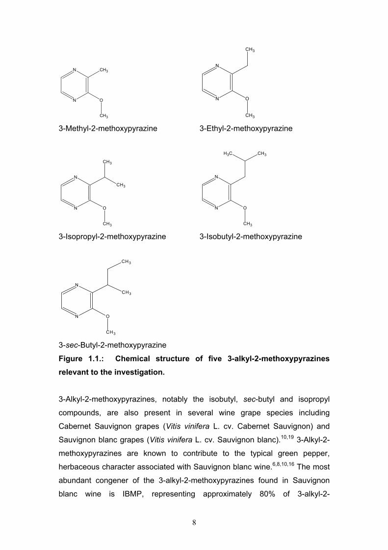
Figure 1.1.: Chemical structure of five 3-alkyl-2-methoxypyrazines relevant to the investigation.

3-Alkyl-2-methoxypyrazines, notably the isobutyl, sec-butyl and isopropyl

compounds, are also present in several wine grape species including

Cabernet Sauvignon grapes (Vitis vinifera L. cv. Cabernet Sauvignon) and

Sauvignon blanc grapes (Vitis vinifera L. cv. Sauvignon blanc).10,19 3-Alkyl-2-

methoxypyrazines are known to contribute to the typical green pepper,

herbaceous character associated with Sauvignon blanc wine.6,8,10,16 The most

abundant congener of the 3-alkyl-2-methoxypyrazines found in Sauvignon

blanc wine is IBMP, representing approximately 80% of 3-alkyl-2-

9

methoxypyrazines commonly found in wine.6,10,19 Studies also demonstrated

that IBMP is the main contributor to the vegetal aroma in Sauvignon blanc

wine.6,8 The fact that IBMP is also the dominant congener in green peppers,

may explain the supposed use thereof in the adulteration of wine. The other

major 3-alkyl-2-methoxypyrazines commonly found in wine, SBMP and IPMP,

each represent approximately 10% of the total 3-alkyl-2-methoxypyrazines in

wine.10,19 The occurrence of EMP in Sauvignon blanc have also been

tentatively reported while the possible occurrence of MMP has been

suggested based upon a feasible biosynthetic route.10 Although it is unlikely

that EMP and MMP may make a significant contribution to Sauvignon blanc

aroma, due to their high odor detection thresholds, they were nevertheless

tentatively included in the investigation. If present at all, the levels of EMP and

MMP may possibly be attenuated by adulteration of Sauvignon blanc wine

with fruit extracts.

The olfactory threshold at which these compounds are sensed is

extraordinarily low, values ranging from 0.5 to 2 ng/L in water are reported in

the literature for the alkylmethoxypyrazines.16,19,20,24 The detection threshold

of IBMP in red wine is 10 to 15 ng/L while 1 to 2 ng/L has a significant

influence on the aroma of a methoxypyrazine-free white wine.8,19,20,24 The

ability of a specific compound to impact the aroma of a wine depends on the

specificity of the aromatic note of such a compound.25 In addition to the fact

that the vegetable character of wine may primarily be attributed to the

presence of IBMP, Ferreira et al. reported that other volatile wine aroma

compounds may synergistically interact with IBMP to significantly enhance the

perceived pepper odor nuance.26 On the contrary, components such as fusel

alcohols, acids, esters, ß-damascenone and some volatile phenols are not

able to individually affect the aroma of wine even if they are present at

concentrations well above their odor thresholds.25 It may therefore be

concluded that IBMP, present at levels of the order of a few parts per trillion,

may have a significant impact on the aroma of Sauvignon blanc wine.

Methoxypyrazine concentrations in grapes are influenced by a multiplicity of

factors including grape variety, fruit maturity, season, climate and solar

10

exposure of the fruit.6,9,19 South African Sauvignon blanc wines contain

approximately < 1 to 14 ng/L of IBMP and often possess very little or no

cultivar character as far as the typical grassy, green pepper aroma is

concerned.6 As the minor 3-alkyl-2-methoxypyrazines are expected to be

present at levels of no more than approximately 10% of that of IBMP, these

may occur at levels of the order of < 0,1 to 2 ng/L respectively, but no relevant

quantitative data are currently available.19 Australian Sauvignon blanc wine,

produced under similar climatological conditions, contains approximately 2 to

15 ng/L of IBMP.6 France and New Zealand, which have cooler climates and

are famous for producing high quality Sauvignon blanc wines, typically range

from 5 to 40 ng/L and 10 to 35 ng/L IBMP respectively.6,12

1.4. Analytical methodologies for the analysis of methoxypyrazines in wine

Several analytical methodologies have been employed successfully for the

measurement of selected 3-alkyl-2-methoxypyrazines in wine. These

exclusively comprise gas chromatography, either in conjunction with mass

spectrometric detection 10,18,24,27,28,29 or nitrogen-phosphorous selective

detection (NPD).20,27 Due to the very low levels of the analytes, sample pre-

concentration is indispensable in all methods used. Sample preparation

generally involves clean-up and pre-concentration utilizing various techniques

including liquid-liquid extraction 10,18,24,28,29,30 distillation 10,18,20,28,29, solid phase

extraction 10,18,28,29 and ionic strength adjustment for the headspace

techniques.20,27 Sample introduction commonly entails splitless injection of

concentrated extracts 10,18,24,29,30 or headspace solid phase micro-extraction

(SPME) utilizing various fibers.20,27 An internal standard is universally used in

conjunction with the various gas chromatographic techniques while the choice

of internal standard varied between deuterium labeled analogs 10,18,27,28,30 and

differently substituted pyrazines.20,24,29 Table 1.3. presents a concise summary

of some methods of analysis reported for the determination of various 3-alkyl-

2-methoxypyrazines in wine.

Table 1.3.: Summary of methods reported in the literature for the analysis of methoxypyrazines in wine.

Author Analysis technique Sample preparation and introduction

Detection Analytes Performance of the method

Kotseridis et al.24

Capillary gas chromatography (cGC) utilizing Carbowax-20M phase and MMP as internal standard.

Solvent extraction with diethyl ether-hexane (1/1, v/v). Splitless injection of concentrated sample extract.

Mass spectrometer operating in selected ion monitoring (SIM) mode.

IBMP MQL:b 2 ng/L

Sala et al.20

cGC utilizing two phases for compound identification, CP-Wax and SPB-35. IPEPa internal standard.

Headspace solid phase micro-extraction (SPME) utilizing a 65 µm PDMS/DVB fiber. Samples were acidified and distilled followed by neutralization and ionic strength adjustment prior to SPME sampling.

Nitrogen Phosphorous Detector (NPD)

IBMP, SBMP, IPMP, EMP

MDL:c 0.3 ng/L (IBMP, IPMP and SBMP). 1.0 ng/L (EMP), (S/N = 3:1)

Roujou de Boubee et al.18

cGC utilizing a BP20 phase and deuterium labeled IBMP as internal standard.

Steam distillation of samples after pH adjustment with NaOH, extraction of distillate with cation exchange resin, elution with 10% NaOH and finally extraction of aqueous phase with dichloromethane. Splitless injection of concentrated sample extract.

Chemical ionization mass spectrometry. Scan mode (m/z 165 - 172)

IBMP Calibration started at 2 ng/L.

Ryan et al.27

Two-dimensional gas chromatography utilizing BPX5 and BP20 phases. d3-IBMP utilized as internal standard.

Headspace SPME utilizing a 65 µm PDMS/DVB fiber and ionic strength adjustment of samples.

Time-of-flight mass spectrometry (utilizing d3-IBMP internal standard) and NPD

IBMP, SBMP

MDL(TOF): 1.96 ng/L MDL(NPD): 0.5 ng/L (IBMP only)

Kotseridis et al.30

cGC utilizing Carbowax-20M phase and deuterium

Solvent extraction with diethyl ether-hexane (1/1, v/v). Splitless

Mass spectrometer operating in SIM

IBMP MQL: 2 ng/L (S/N = 3:1)

12

labeled IBMP as internal standard.

injection of concentrated sample extract.

mode.

Lacey et al.10

cGC utilizing deuterium labeled IBMP and IPMP as internal standards.

Distillation of samples followed by extraction of the distillate with cation exchange resin. Resin washed with 15% NaOH and finally extraction from aqueous phase with dichloromethane. Splitless injection of concentrated sample extract.

Mass spectrometry. IBMP IPMP SBMP

MDL: 0.15 ng/L

Allen et al.28

cGC utilizing BP 5, DB-1, DB-1701 and DB-Wax phases and deuterium labeled IBMP as internal standard.

Distillation of samples (pH 6) followed by extraction of the distillate with cation exchange resin. Resin washed with 10% NaOH and finally extraction of aqueous phase with dichloromethane. Cold on-column injection of concentrated sample extract.

Mass spectrometry (SIM).

IBMP IPMP

Variable, < 1 ng/L

Hashizume et al.29

cGC utilizing a DB-Wax phase and 2-Methyl-3-n-propylpyrazine as internal standard.

Steam distillation of samples (pH 5) followed by extraction of the distillate with ion exchange resin. Resin washed with 20% KOH / 1 M Na2CO3, extraction of aqueous phase with dichloromethane. Splitless injection of concentrated sample extract.

Mass spectrometry (SIM).

IBMP IPMP

0.2 ng/kg (grapes)

a = 3-Isopropyl-2-ethoxypyrazine b = Minimum quantification limit c = Minimum detection limit .

13

1.5. Detection of adulteration: Characterization of the profile of relative abundance of the major 3-alkyl-2-methoxypyrazines in Sauvignon blanc wine

At present, an unambiguous method for the detection of adulteration of South

African Sauvignon blanc wine by fraudulent enrichment of the levels of 3-alkyl-2-

methoxypyrazines, does not exist. South African regulatory laboratories, tasked

with auditing the Sauvignon blanc industry, utilize the method of Kotseridis et

al.24 to build a historical database of quantitative data pertaining specifically to 3-

isobutyl-2-methoxypyrazine. Possible cases of adulteration are identified by

evaluation of the relevant quantitative data for the region and vintage and

comparison with the database of expected values. Due to the variable natural

abundance of 3-isobutyl-2-methoxypyrazine in South African Sauvignon blanc

wine, a strategy of analyzing the IBMP content of must samples prior to alcoholic

fermentation and the final product, has recently been employed in an effort to

detect possible cases of adulteration. As IBMP can only be produced while the

grapes are on the vine, unexplained increases in the quantity of IBMP during the

winemaking process may then provide conclusive evidence of adulteration.

The method of Kotseridis et al.24 (MQL = 2 ng/L) is only suitable for the

determination of IBMP in South African Sauvignon blanc wines and is not

generally applicable for the determination of 3-alkyl-2-methoxypyrazines at their

natural levels of occurrence. Insufficient data pertaining to the relative abundance

of 3-alkyl-2-methoxypyrazines in South African Sauvignon blanc wine is therefore

currently available.

The characteristic cultivar character associated with Sauvignon blanc wine is in

part attributed to certain methoxypyrazines, of which IBMP is the most

important.6,8,9 It may be expected that the other 3-alkyl-2-methoxypyrazine

congeners that are present in Sauvignon blanc grapes, such as IPMP and

SBMP, contribute to the typical green pepper, herbaceous nuances that

14

distinguishes the variety, as these may be present at levels above their sensory

thresholds.8,10,19 As different grape cultivars have distinctive sensory properties, it

may reasonably be assumed that Sauvignon blanc wine contain these congeners

in distinct relative amounts, causing the varietal distinction. This assumption is

supported by the findings of Lacey et al. who reported that that the relative

proportions of three methoxypyrazines in Sauvignon blanc wine of Australian,

New Zealand and French origin are fairly constant and that the relative

abundance of IBMP to IPMP is approximately 7:1.10 Allen et al. similarly found

that the typical abundance of SBMP in some red wines are approximately 2% of

that of IBMP.28 Murray et al. reported that greenpeppers contains the three

relevant methoxypyrazine congeners in fixed relative amounts and that a ratio of

approximately 100:1 exists for IBMP to IPMP.17

A possible strategy for the detection of adulteration may therefore be to

characterize the profile of relative abundances of 3-alkyl-2-methoxypyrazines in

South African Sauvignon blanc wine. If the ratios are found to be consistent, then

samples from all regions producing Sauvignon blanc wine should be analysed to

determine the amount of variance in the typical pattern so that parameters may

be established for authentication of South African Sauvignon blanc wine in this

regard. Quantitative data for the different congeners may also be used as

supplementary information in cases where adulteration is suspected. Green

pepper extracts as well as commercial synthetic preparations should also be

analysed to determine the expected effect of adulteration on the typical

methoxypyrazine profile.

The investigation may be complicated by the fact that wine, labelled as a single

cultivar product, may contain small amounts of wine from a different cultivar.

Current South African legislation, effective from January 2006, stipulates that at

least 85% of the contents of a single cultivar product shall be derived from

grapes of that cultivar. Legislation effective up to December 2005, required that

75% of the contents of a single cultivar wine be derived from grapes of that

15

cultivar.14 This implies that, depending on the vintage, single cultivar products

may contain up to 25% of wine from a different cultivar. The fact that Sauvignon

blanc wines may contain undisclosed amounts of wine from other cultivars, may

affect the amount of variance in the relative abundances of the 3-alkyl-2-

methoxypyrazines, if a pattern is found to exist.

The timing of the harvest is of critical importance from a viticultural point of view

as this determines the properties of the fruit, such as the balance between the

natural accumulated sugars and acids, which sets the limit on the potential

quality of the wine.1,5 Some producers of Sauvignon blanc wine in South Africa

follow a practice of selective and repeated harvesting to obtain fruit possessing

distinct qualities. In the warmer wine-producing regions of South Africa, the IBMP

content of Sauvignon blanc grapes decrease during ripening.9 A proportion of the

fruit may therefore be harvested before it has reached optimal maturity to ensure

high levels of IBMP. A varietal-typical product may thus be obtained by

combining the grapes, which were harvested at different times. This practice may

clearly affect the levels of the 3-alkyl-2-methoxypyrazines in the product and

possibly their relative abundances.

The overall objectives of the study are therefore to establish a method for

elucidation of authenticity of South African Sauvignon blanc wine, specifically

regarding enrichment with foreign 3-alkyl-2-methoxypyrazines, and to perform an

audit of the industry in this regard. Within this context, the following goals were

identified:

1. The implementation of an analytical procedure for the quantitation of

various 3-alkyl-2-methoxypyrazines in South African Sauvignon blanc

wines. This procedure should be capable of accurate and precise

measurements in a concentration range of approximately 0.1 to 50 ng/L.

16

2. Analysis of Sauvignon blanc wine samples representative of the South

African industry to determine the absolute levels of 3-alkyl-2-

methoxypyrazines and possible ratios of relative abundance that may exist

between the various congeners as well as the amount of variance across

the typical spectrum of wines. The expected effect of adulteration with

green pepper extracts and synthetic green pepper flavor preparations, on

the typical spectrum, should also be determined by characterization of the

relative abundance in the mentioned substances.

3. Use of this information to establish parameters that may be used to

discriminate adulterated wine and to predict the effect of adulteration with

green peppers and synthetic green pepper flavor preparations, on the

relative abundance of various 3-alkyl-2-methoxypyrazines in Sauvignon

blanc wine.

1.6. Proposed methodology for characterizing the profile of 3-alkyl-2-methoxypyrazines in South African Sauvignon blanc wine

A major factor that challenges the investigation of wine flavor and aroma are the

extremely low concentrations of the wine flavor components. The concentration

of the various 3-alkyl-2-methoxypyrazines in South African Sauvignon blanc wine

are expected to be in the range of approximately < 0,1 to 14 ng/L.6 Such low

levels necessitate highly sensitive and selective extraction and analysis methods

for quantitative purposes. Chemical changes that occur during aging are not

expected to complicate the investigation. De Boubee et al. reported that the

IBMP content of one Cabernet Sauvignon and one Sauvignon blanc wine

remained unchanged during bottle ageing for three years in a dark cellar.21

Due to the very low and variable concentrations expected for the 3-alkyl-2-

methoxypyrazines in wine, an efficient sample clean-up and pre-concentration

17

step is essential for the successful measurement of the substances under

investigation. The sample preparation procedure should offer quantitative pre-

concentration of the analyte and be robust in order to be suitable for the analysis

of large numbers of samples. Various sample preparation techniques were

evaluated for this purpose including solvent extraction, distillation, solid phase

extraction (SPE), and stir bar sorptive extraction (SBSE). Solvent extraction, in

combination with distillation, was finally selected as the sample preparation

technique as it is particularly suitable for the isolation and pre-concentration of

trace quantities of a species.31

Liquid chromatography-mass spectrometry (LC-MS) was selected as the

analytical technique for measuring the levels of 3-alkyl-2-methoxypyrazines

despite the fact that practically all relevant publications report the use of gas

chromatography for this purpose. The LC-MS mass selective detector offers

sensitivity and selectivity of the same order as equivalent gas chromatography

mass spectrometry (GC-MS) detectors. The liquid chromatographic technique

however offers advantages over gas chromatography such as higher sample

loading capacity and superior sample introduction precision. The latter obviates

the requirement for an internal standard for quantitation as is the case with gas

chromatography. Liquid chromatography is also better suited for the analysis of

thermally unstable components and can accommodate acids and non-volatile

solvents, which may be indispensable as part of an efficient sample preparation

procedure. Very high electrospray ionization efficiencies, up to 100%, have

recently been reported for LC-MS. The compounds of interest are also aromatic,

incorporating heteroatoms with lone pairs of electrons in their ring structure, and

contain electron donating methoxy groups and alkyl side-chains, structural

characteristics that aid charge stabilization in positive mode ionization. These

factors suggest that the LC-MS technique may provide very efficient and

sensitive detection of the compounds of interest.32 The advantages associated

with the liquid chromatographic technique are therefore expected to outweigh the

superior resolution attainable with gas chromatography so that better overall

18

sensitivity is expected from a LC-MS method. The lower resolving power of liquid

chromatography compared to gas chromatography, may however place

particularly stringent demands on sample clean-up, separation and mass

selective detection processes.

19

REFERENCES

(1) R. S. Jackson, WINE SCIENCE: PRINCIPLES, PRACTICE AND

PERCEPTION, 2 nd ed. (2000), Academic Press, San Diego, 1 - 6.

(2) P. Hands, D. Hughes, NEW WORLD OF WINE FROM THE CAPE OF

GOOD HOPE, (2001), Tien Wah Press (Pte) Tld, Singapore, 1 - 25.

(3) J. Simon, DISCOVERING WINE, (1997), Mitchell Beazley, 25 Victoria

Street, London, SW1H0EX, 147.

(4) H. Jones, P. Docherty, THE NEW SOTHEBY’S WINE ENCYCLOPEDIA,

(1997), Dorling Kindersley Limited, 9 Henrietta Street, London WC2E 8PS,

377.

(5) J. Robinson, THE OXFORD COMPANION TO WINE, 2nd ed. (1999),

Oxford University Press, Great Clarendon Street, Oxford, 3 - 4.

(6) J. Marais, P. Minnaar, F. October, 2-METHOXY-3-ISOBUTYLPYRAZINE

LEVELS IN A SPECTRUM OF SOUTH AFRICAN SAUVIGNON BLANC

WINES, Wynboer (2004).

(7) SOUTH AFRICAN WINE INDUSTRY INFORMATION & SYSTEMS

(SAWIS), S.A. Wynbedryfstatistiek no. 29 (2005), P.O. Box 238, Paarl,

7620, 9 - 14.

(8) M. S. Allen, M. J. Lacey, R. L. N. Harris, W. V. Brown, CONTRIBUTION

OF METHOXYPYRAZINES TO SAUVIGNON BLANC WINE AROMA.

Am. J. of Enol. Vitic., 42 (1991), 109 – 112.

(9) J. Marais, FACTORS AFFECTING SAUVIGNON BLANC WINE QUALITY.

Wynboer 12 (2005), 69 - 70.

(10) M. J. Lacey, M. S. Allen, R. L. N. Harris, W. V. Brown,

METHOXYPYRAZINES IN SAUVIGNON BLANC GRAPES AND WINE.

Am. J. Enol. Vitic., 42 (1991), 103 – 108.

(11) P. Hands, D. Hughes, WINES AND BRANDIES OF THE CAPE OF GOOD

HOPE, Stephan Phillips Publishers, 69.

(12) J. Halliday, H. Johnson, THE ART AND SCIENCE OF WINE (2000),

Mitchell Beazley, Hong Kong, 34 - 35.

20

(13) C. Du Plessis, GEURMIDDEL-SKADE GROOTLIKS BEPERK, Wineland,

(2005).

(14) LIQUOR PRODUCTS ACT, Act 60 (1989), Government Gazette of the

Republic of South Africa.

(15) J. A. Maga, C. E. Sizer, PYRAZINES IN FOODS. A REVIEW. J. Agr.

Food Chem., 21 (1973), 22 – 30.

(16) C. Sala, O. Busto, J. Guasch, F. Zamora, CONTENTS OF 3-ALKYL-2-

METHOXYPYRAZINES MUSTS AND WINES FROM VITIS VINIFERA

VARIETY CABERNET SAUVIGNON: INFLUENCE OF IRRIGATION AND

PLANT DENSITY, J. Sci. Food. Agric., 85 (2005), 1131 – 1136.

(17) K. E. Murray, F. B. Whitfield, THE OCCURRENCE OF 3-ALKYL-2-

METHOXYPYRAZINES IN RAW VEGETABLES, J. Sci. Food. Agric., 26

(1975), 973 – 986.

(18) D. Roujou De Boubee, C. Van Leeuwen, D. Dubourdieu,

ORGANOLEPTIC IMPACT OF 2-METHOXY-3-ISOBUTYLPYRAZINE ON

RED BORDEAUX AND LOIRE WINES, EFFECT OF ENVIRONMENTAL

CONDITIONS ON CONCENTRATIONS IN GRAPES DURING

RIPENING, J. Agric. Food Chem., 48 (2000), 4830 – 4834.

(19) P. J. Hartmann, THE EFFECT OF WINE MATRIX INGREDIENTS ON 3-

ALKYL-2- METHXYPYRAZINES MEASUREMENTS BY HEADSPACE

SOLID-PHASE MICROEXTRACTION (HS-SPME), (2003), Virginia

Polytechnic Institute and State University, Blacksburg, Virginia.

(20) C. Sala, M. Mestres, M.P. Marti, O. Bustro, J. Guasch, HEADSPACE

SOLID-PHASE MICROEXTRACTION OF ANALYSIS OF 3-ALKYL-2-

METHOXYPYRAZINES IN WINE, J. Chromatogr. A, 953 (2002), 1 – 6

(21) D. Roujou De Boubee. RESEARCH ON 2-ALKYL-3-

METHOXYPYRAZINES IN GRAPES AND WINES. School of Oenology,

University of Bordeaux.

(22) Z. Rappoport, CRC HANDBOOK OF TABLES FOR ORGANIC

COMPOND IDENTIFICATION. 3rd ed. CRC Press, Inc. Boca Raton,

Florida.

21

(23) D. R. Lide, CRC HANDBOOK OF CHEMISTRY AND PHYSICS, 86th ed.

(2005 – 2006), CRC Press, 6000 Broken Sound Parkway NW, Suite 300

Boca Raton FL.

(24) Y. Kotseridis, A. Anocibar Beloqui, A. Bertrand, J. P. Doazan, AN

ANALYTICAL METHOD FOR STUDYING THE VOLATILE

COMPONENTS OF MERLOT NOIR CLONE WINES Am. J. Enol. Vitic.

49 (1998), 44 – 48.

(25) A. Escudero, B. Gogorza, M.A. Melus, N. Ortin, J. Cacho, V. Fereirra.

CHARACTERIZATION OF THE AROMA OF A WINE FROM

MACCABEO. KEY ROLE PLAYED BY COMPOUNDS WITH LOW ODOR

ACTIVITY VALUES. J. Agric. Food Chem., 52 (2004), 3516 - 3524.

(26) A. Escudero, E. Campo, L. Farina, J. Cacho, V. Ferreira, ANALYTICAL

CHARACTERIZATION OF THE AROMA OF FIVE PREMIUM RED

WINES. INSIGHTS INTO THE ROLE OF ODOR FAMILIES AND THE

CONCEPT OF FRUITINESS OF WINES. J. Agric. Food Chem., 55

(2007), 4501 - 4510.

(27) D. Ryan, P. Watkins, J. Smith, M. Allen. P. Marriott, ANALYSIS OF

METHOXYPYRAZINES IN WINE USING HEADSPACE SOLID PHASE

MICROEXTRACTION WITH ISOTOPE DILUTION AND

COMPREHENSIVE TWO-DIMENSIONAL GAS CHROMATOGRAPHY. J.

Sep. Sci., 28 (2005), 1075 - 1082.

(28) M. S. Allen, M. J. Lacey, S. Boyd, DETERMINATION OF

METHOXYPYRAZINES IN RED WINES BY STABLE ISOTOPE

DILUTION GAS CHROMATOGRAPHY-MASS SPECTROMETRY. J. Agr.

Food Chem., 42 (1994), 1734 - 1738.

(29) K. Hashizume, T. Samuta, GRAPE MATURITY AND LIGHT EXPOSURE

AFFECT BERRY METHOXYPYRAZINE CONCENTRATION. Am. J. Enol.

Vitic., 50 (1999), 194 – 198.

(30) Y. Kotseridis, R. L. Baumes, A. Bertrand, G. K. Skouroumounis,

QUANTITATIVE DETERMINATION OF 2-METHOXY-3-

ISOBUTYLPYRAZINE IN RED WINES AND GRAPES OF BORDEAUX

22

USING A STABLE ISOTOPE DILUTION ASSAY. J. Chromatogr., 841

(1999), 229 - 237.

(31) D. A. Skoog, D.M. West, F.J. Holler, FUNDAMENTALS OF ANALYTICAL

CHEMISTRY 7th ed.(1996), Saunders College Publishing, Orlando, 760 -

777.

(32) G. J. Van Berkel, V. Kertesz, USING THE ELECTROCHEMISTRY OF

THE ELECTROSPRAY ION SOURCE, Analytical Chemistry, (2007), 5510

- 5520.

23

CHAPTER 2

Analytical techniques

2.1. Introduction

Generally, methods for chemical analysis are at best selective, few are truly

specific. Consequently, separation of analytes from potential interferences is

vitally important in analytical investigations.1 This requirement becomes even

more important in trace level analysis where the concentration of the analyte,

relative to sample matrix components, may be exceedingly small. Modern

analytical separations are most commonly performed using chromatography and

electrophoresis. Especially the modern versions of high performance liquid

chromatography (HPLC) and capillary gas chromatography (cGC) are by far the

most widely used separation techniques.1,2,3

In this Chapter an overview of the analytical techniques relevant to the study are

presented. Apart from a broad introduction to chromatography, the focus of the

discussion will primarily be on liquid chromatography and more specifically on the

techniques used for analyses of residues in this study. A brief overview of gas

chromatographic techniques, relevant to the study, will also be presented.

2.2. General description of chromatography

In chromatographic separations the sample or analyte molecules are transported

in a mobile phase through an immiscible stationary phase, which is fixed in a

column or on a solid surface. The sample is dissolved in the mobile phase, which

may be a gas, a liquid or a supercritical fluid. The two phases are selected to

ensure that components of the sample distribute themselves between the mobile

24

phase and the stationary phases to varying degrees. With the flow of the mobile

phase, those components that are retained weakly by the stationary phase elute

from the system before strongly retained components. As a consequence of

these differences in mobility, components may be separated into discrete bands

that can be analyzed quantitatively and/or qualitatively.1,2,3,4,5

Chromatographic methods are categorized based upon the physical means by

which the mobile and stationary phases are brought together. In column

chromatography, the stationary phase is held in a tube, generally referred to as a

column, through which the mobile phase is forced under pressure or gravity. In

planar chromatography, the stationary phase is supported on a flat surface

through which the mobile phase moves by capillary action or under the influence

of gravity. Separation in both planar and column chromatography are based upon

the same chemical equilibria.1,2,3,4,5 A more fundamental classification of column

chromatographic methods is based on the types of mobile and stationary phases

and the equilibria involved in the transfer of solutes between the phases, as is

shown in Table 2.1.

25

Table 2.1.: Classification of the most common column chromatographic separations.1

Classification Method Stationary phase Equilibrium Liquid-liquid or partitioning

Liquid adsorbed on solid

Partition between immiscible liquids

Liquid-bonded phase

Organic species bonded to solid

Partition between liquid and bonded phase

Liquid-solid or adsorption

Solid Adsorption

Ion exchange Ion exchange resin Ion exchange

Liquid chromatography

Size exclusion Liquid in interstices of polymeric solid

Partition/sieving

Gas-liquid Liquid adsorbed on solid

Partition between gas and liquid

Gas-bonded phase


Partition between gas and bonded phase

Gas chromatography

Gas-solid Solid Adsorption Supercritical fluid-bonded phase


Partition between super-critical fluid and bonded surface

Supercritical-fluid chromatography

Supercritical fluid-solid

Solid Adsorption

2.2.1. Migration rates of solutes in chromatographic separations

Chromatographic separation depends on the relative rates at which different

solutes move down the column. These rates are determined by the equilibrium

constants for the reactions by which the solutes distribute themselves between

the mobile and stationary phases. The distribution constant, K is described by the

equation:

K = cS/cM (1)

where cS and cM is the molar concentration of the solute in the mobile and

stationary phases, respectively. Ideally, K is constant over a wide range of solute

concentrations which results in characteristics such as symmetric Gaussian type

peaks and retention times that are independent of solute concentration.1

26

The retention factor, k’, is defined as the time that the solute spends in the

stationary phase relative to the time it spends in the mobile phase, while

retention time represents the total time that the solute spends in the column.

The retention factor, k’ for solute A is defined as follows:

k’A = (KA VS)/VM = (tR – tM)/tM (2)

where KA is the distribution constant, VS and VM are the phase volume of the

stationary and mobile phases and tR and tM the retention time of the solute and

an unretained peak, respectively. Ideally, separations are performed under

conditions in which the retention factor for the solutes is in the range 2 to 10.1

The selectivity factor, α, of a separation for two species A and B is defined as

follows:

α = KB/KA = ((tR)B – tM)/ ((tR)A – tM) (3)

where KB and KA are the distribution constants for the strongly and less strongly

retained species and tR and tM the retention time of the solute and an unretained

peak respectively.1

The resolution, RS of a column provides a quantitative measure of its ability to

resolve two solutes, A and B, in a mixture:

RS = 2[(tR)B – (tR)A] / (WA + WB) = 2 Δ tR / (WA + WB) (4)

where (tR)B and (tR)A are the retention time of solute A and B and WA and WB, the

width of the peaks at the baseline (Figure 2.1.). A resolution of 1.5 provides

complete baseline separation of two components.1,2,3

27

As the peak widths of two adjacent peaks in high efficiency chromatography are

approximately equal, the resolution equation may also be written in terms of α, k’

and N:

RS = ((N)1/2) / 4 . ((α -1) / α) . (k2 / 1 + k2) (5)

where N is the plate count, α the selectivity factor and k2 the retention factor of

the last eluting solute.2,4

Figure 2.1.: Resolution for Δ tR = 4 σ.* * Introduction to Separation Science, Stellenbosch University 2007, P. Sandra, A.J. de Villiers.

2.2.2. Band broadening in chromatography

In any chromatographic process, separation is generally accompanied by dilution

of the analyte, a phenomenon commonly referred to as band or peak broadening.

28

Peak broadening predominantly occurs as the sample is separated on the

column, but may also occur outside the column. Extra-column band broadening

includes the dilution attributed to the injector, connecting tubing as well as the

detector.1 The discussion that follows pertains specifically to on-column peak

broadening.

Chromatographic peaks generally resemble Gaussian curves because variable

residence time of the solutes in the mobile phase leads to irregular migration

rates with a symmetric spread of velocities around the mean value. The breadth

of a Gaussian curve is directly related to the variance, σ2 of measurement. The

efficiency of a column is therefore conveniently expressed in terms of variance

per unit length. The plate height, H is given by the equation:

H = σ2/L (6)

where L is the length of the column and σ2 carries units of length squared. H

therefore represents a linear distance in centimeters. The plate height may be

thought of as the length of column that contains the fraction of solute that lies

between L – σ and L. The column therefore becomes more efficient with smaller

values of H.1,3

The plate count, N is related to H by the equation:

N = L / H (7)

where L is the length of the column packing. N may also be approximated by

determining W1/2, the width of the peak at half-height. The plate count is then

given by:

N = 5.54 (tR / W1/2)2 (8)

29

where tR is the retention time of the peak. The efficiency of the chromatographic

column increase as the plate count becomes greater. The plate count N and

plate height H may be used to measure column performance. Where two

columns are compared, the same compound should be used in determining

these parameters.1

Peak broadening during the chromatographic separation is the consequence of

longitudinal diffusion, multiple flow paths through a packed bed and the finite rate

at which several mass-transfer processes occur. The contribution of each of

these processes to the plate height is described by the Van Deemter equation:

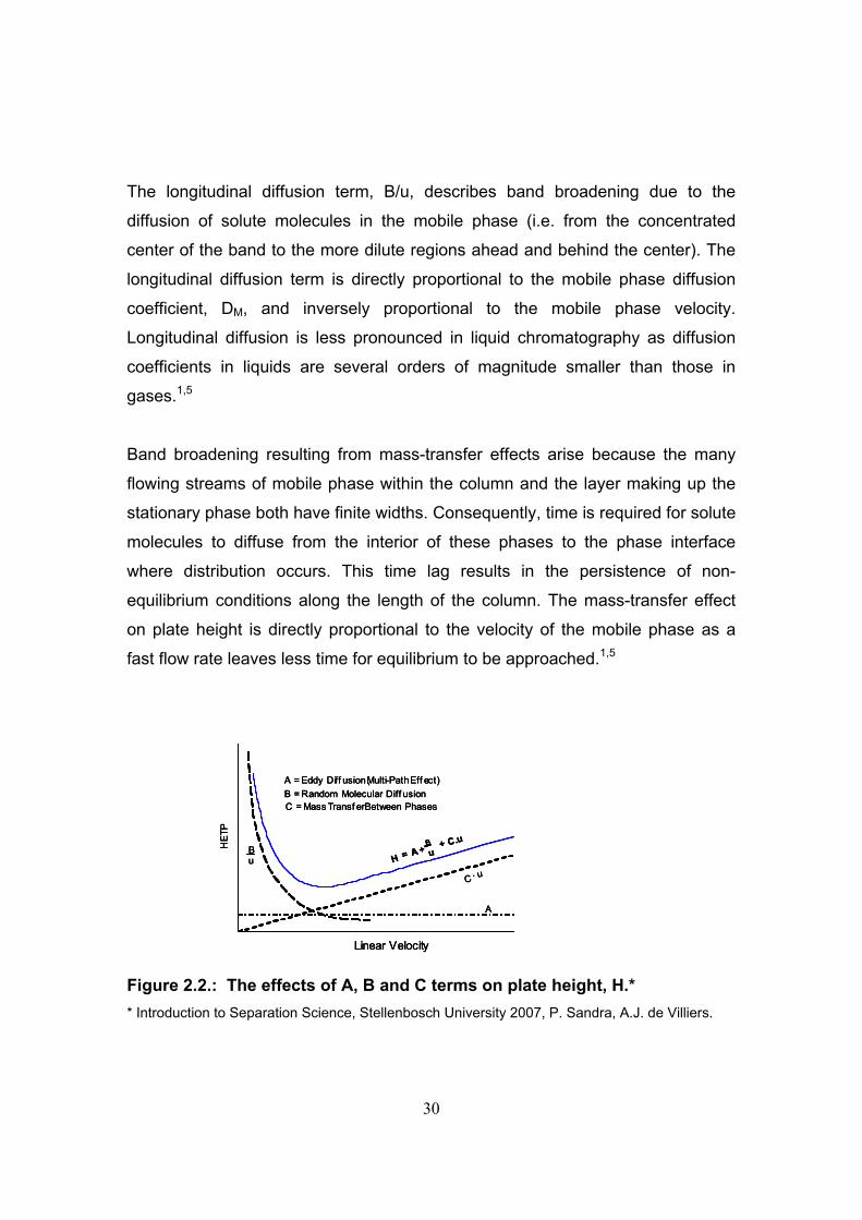
H = A + B/u + (C)u (9)

where u is the linear velocity of the mobile phase and the coefficients A, B and C

are related to the phenomena of multiple flow paths, longitudinal diffusion and

mass-transfer between the phases, respectively.1,3,4,5 Figure 2.2. graphically

relates these factors to plate height (H).5

The multi-path term, A describes peak broadening that results from the multitude

of pathways by which a solute molecule can find its way through a packed bed.

Due to the variable lengths of these pathways, the residence time in the column

for molecules of the same species differ. Solute molecules therefore reach the

end of the column over a time interval, which leads to peak broadening. This

effect, also called eddy diffusion, is directly proportional to the diameter of the

packing particles. Multi-path peak broadening may be partially offset by ordinary

diffusion, which results in the transfer of molecules from a stream following one

pathway to a stream following anther pathway. At very low velocities, a large

number of these transfers occur so that numerous pathways are sampled by

each molecule and the rate at which each molecule moves down the column

tends to approach the average. At moderate to high velocities, sufficient time for

diffusion averaging is not available and band broadening is observed.1,3

30

The longitudinal diffusion term, B/u, describes band broadening due to the

diffusion of solute molecules in the mobile phase (i.e. from the concentrated

center of the band to the more dilute regions ahead and behind the center). The

longitudinal diffusion term is directly proportional to the mobile phase diffusion

coefficient, DM, and inversely proportional to the mobile phase velocity.

Longitudinal diffusion is less pronounced in liquid chromatography as diffusion

coefficients in liquids are several orders of magnitude smaller than those in

gases.1,5

Band broadening resulting from mass-transfer effects arise because the many

flowing streams of mobile phase within the column and the layer making up the

stationary phase both have finite widths. Consequently, time is required for solute

molecules to diffuse from the interior of these phases to the phase interface

where distribution occurs. This time lag results in the persistence of non-

equilibrium conditions along the length of the column. The mass-transfer effect

on plate height is directly proportional to the velocity of the mobile phase as a

fast flow rate leaves less time for equilibrium to be approached.1,5

H = A + + C.uHE

TP

Bu

C. u

A

Linear Velocity

A = Eddy Diff usion(Multi-PathEff ect)B = Random Molecular Diff usionC = Mass Transf erBetween Phases

BuH = A + + C.uH

ETP

Bu

C. u

A

Linear Velocity


BuH = A + + C.uH

ETP

Bu

C. u

A

Linear Velocity


Bu

Figure 2.2.: The effects of A, B and C terms on plate height, H.* * Introduction to Separation Science, Stellenbosch University 2007, P. Sandra, A.J. de Villiers.

31

2.2.3. Optimization of chromatographic resolution

A chromatographic separation is optimized by varying experimental conditions

until the components of a mixture are separated efficiently with a minimum

expenditure of time. In seeking optimum conditions for achieving a desired

separation, the fundamental parameters pertaining to retention (k’), selectivity

(α), and efficiency (N or H), may be adjusted. Optimization experiments are

therefore aimed at altering the relative migration rates of solutes and at reducing

peak broadening.1

Peak resolution, Rs, as expressed in terms of α, k’ and N may therefore be

optimized by manipulating each of these variables (equation 5).

Peak resolution is proportional to the square root of the plate number. A fourfold

increase in the plate number therefore doubles the peak resolution. Resolution

may therefore be optimized by increasing the plate number or by optimizing the

plate height. The plate number may be increased by using longer columns while

the plate height may be reduced by using smaller diameter columns in gas

chromatography or by reducing the particle size in liquid chromatography. The

plate height may also be reduced by optimizing the mobile phase velocity.

Optimization of the selectivity factor has the largest effect on resolution.

Selectivity may be optimized by changing the stationary phase in gas

chromatography while the stationary as well as the mobile phases may be

altered in liquid chromatography to optimize selectivity.

For values above 5, the influence of the retention factor, k, on resolution is small.

On the other hand, low k values result in poor peak resolution. In gas

chromatography the retention factor may be increased by decreasing the column

temperature, changing the stationary phase or increasing the phase ratio, while

32

in liquid chromatography the mobile phase, stationary phase or phase ratio may

be altered to optimize the retention factor.1,4

2.2.4. Differences between liquid chromatography and gas chromatography

Focusing on liquid and gas chromatography, the most prevalent forms of

chromatographic separations, some pertinent differences can be highlighted.

The high diffusion rates and low viscosity of gaseous separations inherently lend

them to the use of capillary columns. Thin columns (commonly 250-320 μm i.d.)

coated with a thin layer of liquid stationary phase are therefore used in modern

gas chromatography. In liquid chromatography, by comparison, analyte diffusion

and mobile phase viscosity are two orders of magnitude lower and higher,

respectively, compared to gas chromatography. As a consequence, packed

columns are used in liquid chromatography, where small particles are used to

reduce the diffusion distances. As a direct result, high pressures are required to

force the highly viscous liquid mobile phase through a packed bed.

Moreover, in gas chromatography, the mobile phase is an inert gas and no

interactions take place between the solute and the mobile phase, so that

separation is essentially a function of interactions between the solute and the

stationary phase. As separation is performed in the gas phase, the distribution

between the two phases is significantly affected by the volatility of the analyte,

and therefore by the temperature. In fact, in the absence of specific interactions

with the stationary phase, as commonly occurs when using apolar phases,

separation is primarily based on differences in vapor pressures, with analytes

eluting in sequence of increasing boiling point. For this reason, temperature

programming is commonly used to regulate retention in GC separations.

33

In liquid chromatography an interactive mobile phase is utilized, which provides

an additional parameter for selectivity tuning as separation is the result of

interactions of the solute with both the mobile and stationary phases.

Accordingly, mobile phase gradients are most often used to control analyte

retention in HPLC.

In the following sections column characteristics, separation modes and

instrumental aspects will be discussed briefly for liquid and gas

chromatography.1,6,7

2.3. High performance liquid chromatography

Early liquid chromatographic separations were performed in large diameter glass

columns packed with relatively large diameter stationary phase particles.

Decreasing the particle size of columns affected vast increases in efficiency but

required sophisticated instruments operating at high pressure. High performance

liquid chromatography, HPLC, is the term used to distinguish these modern

instrumental liquid chromatographic techniques from classical gravity flow- and-

thin layer liquid chromatography. HPLC is currently the most widely used

analytical separation technique, mainly as a result of its broad applicability and

amenability to accurate and sensitive analysis.1

2.3.1. The HPLC column

The heart of the HPLC system is the column, where the actual separation of

sample components occurs. Modern HPLC columns consist of heavy-walled

stainless steel tubes (Figure 2.3.) pressure packed with fine-diameter packing

material, and equipped with inlet and outlet fittings for incorporation into the

system between the injector and detector.8

34

Macroporous silica gel is by far the most important adsorbent for liquid-solid

chromatography and is also the material used to prepare most bonded phase

packings. Silica particles can be produced reliably with defined particle size, are

physically stable at high pressures, porous to increase sample capacity and can

easily be derivatized with different materials to tune the selectivity.3

Figure 2.3.: HPLC columns, guard column (disposable cartridge and holder) and connector.* * Agilent Technologies Inc., Waldbronn, Germany.

2.3.2. Column efficiency in HPLC

Plate numbers for liquid chromatographic columns are an order of magnitude

smaller than those encountered with gas chromatographic columns. This is

largely due to the pressure drop in liquid chromatography, which limits the

potential length of packed columns. Gas chromatographic columns, which may

be as long as 60 m, provide a larger number of theoretical plates and superior

efficiency. Nonetheless, with two interactive phases and a diversity of stationary

phases, HPLC offers a variety of variables that may be manipulated to optimize

separation selectivity (the α factor) to separate complex mixtures.1

35

Adjustment of the solvent composition, in terms of the types of solvent as well as

their relative proportions in the mobile phase, permits manipulation of k’ and α to

resolve the components in a mixture. The resolution may also be improved by

increasing N, by lengthening the column or more practically, by reducing H. H

may be reduced by reducing the particle size or by altering the flow rate (to

operate at uopt) or viscosity of the mobile phase. Reducing the viscosity affects an

increase in the diffusion coefficient in the mobile phase and may be affected by

elevating the column temperature. Finally, the nature of the interactions with the

stationary phase may be changed by utilizing any of a variety of different

stationary phases.1

Important variables that affect on-column peak broadening in liquid

chromatography are the diameter and size distribution of the packing particles,

diffusion coefficients in the mobile and stationary phases and the flow rate of the

mobile phase.1,8 The Van Deemter equation may be used to relate the

parameters that causes peak broadening to H as a function of mobile phase

velocity, and therefore to optimize these parameters.

2.3.3. Modes of separation in liquid chromatography

All forms of liquid chromatography are differential migration processes where

sample components are selectively retained by a stationary phase. Retention in

liquid chromatography is a complex process involving solute interactions in both

the mobile and stationary phases. Modes of interaction include liquid-liquid

(partition) chromatography, liquid-solid (adsorption) chromatography, ion

exchange chromatography and two types of size exclusion chromatography

namely gel-permeation and gel-filtration chromatography.1,3

36

Reversed phase liquid chromatography (RP-LC) is a form of partition

chromatography which is based on the partitioning of analytes between a

relatively apolar stationary phase and a relatively polar mobile phase and, is the

most widely used separation mode in liquid chromatography. The popularity of

reversed phase liquid chromatography is explained by its unmatched simplicity,

versatility and scope. The near universal application of reversed phase liquid

chromatography stems from the fact that virtually all organic molecules have

hydrophobic regions in their structure and are capable of interacting with the

stationary phase. The rapid equilibration of the stationary phase with changes in

mobile phase composition ensures amenability with gradient elution techniques.3

Reversed phase chromatography is most likely to provide optimum retention and

selectivity where the solutes have limited hydrogen-bonding groups or a

predominant aliphatic- or aromatic character. This mode of liquid

chromatography is particularly well suited for separating solutes based on the

size and structure of alkyl groups and was therefore used exclusively in the

separations performed in this study.3,6 The following discussion will therefore be

limited to reversed phase liquid chromatography.

Retention in reversed phase liquid chromatography occurs by non-specific

hydrophobic interactions of the solute with the stationary phase. Hydrophobic

retention, as encountered in RP-LC, involves mainly apolar compounds or apolar

portions of molecules. Hydrophobic retention is reduced by increasing the

fraction of organic solvent in the aqueous mobile phase. The less polar the

added organic solvent, the greater the effect. The predominant factors that

determines the hydrophobicity of the stationary phase are the length of the alkyl

chain or the total number of carbon atoms as well as the bonding density.3,6,9

In reversed phase liquid chromatography (RP-LC), the apolar, hydrophobic

stationary phase is commonly obtained by chemical derivitization of silica

particles with apolar moieties such as C18 functional groups. The mobile phase

commonly consists of a partially or fully aqueous solution. Elution of the solute is

37

achieved by decreasing the polarity of the mobile phase through increasing the

fraction of organic modifier. Under such conditions, the least polar, hydrophobic

solutes are retained more strongly and display the longest retention times while

polar compounds do not partition to a significant extent into the stationary phase

and elute first. Methanol and acetonitrile are popular solvents because they have

low viscosities, are readily available with excellent purity and are miscible with

water in all proportions. Eluents of intermediate strength between these solvents

and water are usually obtained by mixing these in appropriate ratios.6

Isocratic elution, where the composition of the mobile phase remains unchanged

throughout the separation process, may fail to provide separation of compounds

with widely varying k’ values within an acceptable time. To separate a sample

that contains compounds that are both weakly and strongly retained, the

retention of the individual compounds must be changed during the

chromatographic run, using a process called gradient elution. Gradient elution

involves changing the mobile phase composition, either stepwise or continuously,

during the chromatographic analysis. This process is used to gradually reduce k’

values of the components so that all compounds elute without excessive analysis

time (and band broadening). The small k’ value at the time of elution affects

narrow peakwidths, resulting in increased sensitivity. In reversed phase

chromatography, solvent gradients are generated by increasing the fraction of

organic modifier in the mobile phase.6 Modern HPLC instruments may use up to

four solvents to produce intricate gradients to allow separation of complex

mixtures.

The stationary phase for C18 columns are typically prepared by covalent

attachment of the octadecyl hydrocarbon to silanol groups on the silica support

particles. Bonded-phase packings are relatively stable as the stationary phase is

chemically bound to the solid support. The siloxane (Si-O-Si-R) bond, widely

used for this purpose, is prepared by the reaction of alkoxysilane with surface

silanol groups of hydrolyzed silica gel. For steric reasons, it is not possible for all

38

silanol groups to react and the silica surface consequently consists of a small

percentage of un-derivatized silanol groups in addition to the hydrocarbon

functional groups. Remaining silanol groups may be removed by reaction with a

suitable silylating agent that is able to penetrate the location of the unreacted

silanol groups. This process, known as endcapping, renders the material less

polar, and reduces possible secondary polar interactions. The additional polar

and ionic interactions provided by silanol groups in non-endcapped phases may

enhance selectivity where the solute posses some polar character, but may also

cause unwanted band broadening for basic compounds. The bonded alkyl

phases offer fast analyses and rapid re-equilibration when the mobile phase is

altered, as in gradient elution. The stability of the Si-O-Si bond is dependent the

mobile phase pH and above pH 7, the bonds may be hydrolized with consequent

degradation of the stationary phase.1,6

The main limitation of silica as a support material is the pH range over which it is

stable. Most chemically modified silicas are useful from pH ~2 to 8 and will

experience accelerated degradation outside this range. Polymeric materials

possess wide pH stability and when chemically modified with hydrophobic

functional groups, these materials may be used for reversed phase separations.

Polystyrene-divinylbenzene phase may be used in the manner. The possibility of

utilizing π–π interactions or charge transfer effects with the phenyl phase may

lead to different selectivity than solely hydrophobic interactions. The phase is

suited for non-selective retention of solutes of low to moderate polarity via a

reversed phase mechanism. The large surface area associated with the

polymeric sorbents imparts a relatively high capacity to the phase, although the

tendency of the material to expand and contract in different mobile phase

compositions may lead to non-reproducible chromatographic performance.6,8,9

Ion-pair chromatography, which may be considered to be a version of RP-LC, is

used to separate ionized or ionizable species on reversed phase columns. In ion-

pair chromatography an ion-pairing reagent is added to the mobile phase. The

39

ion-pair reagent possesses both hydrophobic and polar (typically ionic) functional

groups and as a result is retained by the stationary phase, thereby providing the

otherwise apolar stationary phase with an ionic functionality. Most ion-pair

reagents contain alkyl groups to enhance retention on the apolar stationary

phase. The modified stationary phase may then retain and separate organic

solute ions of opposite charge by formation of a reversible ion-pair complexes. At

the same time, the stationary phase is able to retain and separate non-ionized

organic solutes. Ion-pair chromatography thus extends the utility of reversed

phase chromatography to ionic compounds.6

Sample focusing is readily adaptable to reversed-phase chromatography. An

injection solvent such as water that is significantly weaker than the mobile phase

is used to dissolve the sample. Focusing of the solute plug occurs at the head of

the column as the retention of analytes is enhanced under these conditions.

Gradient elution may subsequently be used to separate the sample starting from

a narrow band.6

2.3.4. HPLC instrumentation

An HPLC separation is performed by pumping the mobile phase from a reservoir,

through an optional degasser and injector, into the column, and out to the

detector. The sample, dissolved in a suitable solvent, is introduced into the

flowing mobile phase by making use of the injector. Inside the column, separation

of analyte molecules occurs according to the specific column and mobile phase

combination, following which analytes are eluted from the column and passed

into the detector. The detector generates a signal for the separated compounds

(if detected), which is sent to a suitable data system. The data system then

generates a plot of signal intensity as a function of time – this ‘picture’ of the

separation is called a chromatogram. Figure 2.4. presents a schematic

representation of an HPLC system. Chromatographic data may be quantitative

40

and where the detector is capable of acquiring spectral information of eluted

compounds, qualitative data may be generated at the same time.8 An overview of

the hardware that supports the column in HPLC will be presented with special

reference to the equipment used in this study.

Injector

Detector

Chromatogram

Column

Solvents

Pumps

Mixer

Injector

Detector

Chromatogram

Column

Solvents

Pumps

Mixer

Injector

Detector

Chromatogram

Column

Solvents

Pumps

Mixer

Figure 2.4.: Schematic of HPLC instrument.* * Introduction to Separation Science, Stellenbosch University 2007, P. Sandra, A.J. de Villiers.

2.3.5. Mobile phase treatment system

HPLC instruments are usually equipped with glass reservoirs that contain the

solvents. Dissolved gasses, mostly oxygen and nitrogen, may interfere with the

analysis by forming bubbles in the system. Bubbles may cause the pump to

malfunction, lead to band spreading and interfere with the performance of the

detector.1

Dissolved gasses may be removed by any of a number of strategies. Degassing

may be achieved by sparging, where gasses are swept out of solution by fine

41

bubbles of an inert gas that is not soluble in the mobile phase. Helium is often

used for this purpose. Continuous vacuum degassers use permeable

membranes that separate the mobile phase stream from a vacuum source,

thereby effectively outgassing the mobile phase before it is fed into the pumping

system. Suction filtration also effectively removes dissolved gasses from the

mobile phase in addition to elimination of suspended particles. Degassing of the

mobile phase may also be achieved by sonication, distillation or heating and

stirring.1

2.3.6. Solvent delivery system

The solvent delivery system acquires solvent from the reservoirs through a filter,

pressurizes the solvent sufficiently to overcome resistance from the column

packing material and drives it through the system. The demands placed on an

HPLC solvent delivery system are severe. These include the requirements to

produce a reproducible pulse-free output at pressures up to 400 bar with

accurate flow control at flow rates from 0.1 to 10 mL/min. For gradient elution

precise and accurate control over at least two solvents is desired. The system

should also have a small internal volume for solvent variation in gradient elution

and all components should be corrosion resistant.1

Basic pump designs include the reciprocating piston displacement pump, syringe

pumps and pneumatic or constant pressure pumps.1 As the reciprocating piston

displacement pump is used almost exclusively in modern solvent delivery

systems, the discussion will be limited to this design.

This pump consists of a metal body drilled out to provide a pumping chamber

that is sealed at the back with a Teflon seal through which an inert piston rides.

Pistons are commonly made of beryl glass and are operated by a cam-driven

motor. The inlet and outlet ports are equipped with check-valves that open and

42

close alternately to control the flow of solvent into and out of the cylinder. During

the filling stroke, the inlet check-valve opens to admit solvent to the chamber

while the outlet valve closes to prevent pressurized solvent from re-entering the

chamber. During the pressurization stroke the inlet check-valve closes to prevent

solvent from running back into the reservoir while the outlet valve opens to allow

solvent delivery to the system.8

A problem inherent to this design is that pressure pulses are produced which are

transmitted through the system and negatively affect the analysis in the form of

signal noise. This problem may be minimized by three methods.8 Opposing

multiple pump heads may be used to pressurize the system at different times so

that at any particular time one or the other pump is pressurizing the system. By

arranging the pressurizing cycles of the two pumps so that they are slightly out of

phase, a gradual take-over between the alternate delivery strokes may be

established.6 This method increases the cost of the solvent delivery system, but

produces relatively pulse-free solvent delivery. The system can also be designed

to speed up the refilling stroke with the result that the single pump spends the

majority of its time in the delivery mode. This design is not as efficient as dual-

pump systems, but is less expensive. Pulse dampeners may also be used in

conjunction with dual-pump or single pump systems to reduce pressure pulsation

in the solvent delivery system.8

A separation that employs a single solvent of constant composition is called an

isocratic elution. Separation efficiency may be enhanced by gradient elution

where the solvent delivery system is programmed to mix two or more solvents,

continuously or in a series of steps. Solvents used in the formation of the

gradient may be mixed in two ways, after the pump-heads (high pressure mixing)

or before the pumps (low pressure mixing). High-pressure mixing essentially

combines the output of two isocratic pumps, each dedicated to one solvent. This

system is expensive and essentially restricted to binary gradients, but can

produce sharp, reproducible gradient profiles. Low-pressure mixing employs a

43

proportioning valve between the pump head and the solvent reservoirs and is

capable of mixing more than two channels, but efficient degassing is required for

accurate formation of the gradient.6,8

A small internal volume is critical in pump design as changes in solvent

composition during gradient elution should be rapid and accurate. The capacity

of the pump chamber in most reciprocating piston displacement pumps vary from

approximately 35 to 400 µL which makes this design amenable to gradient

elution techniques.6

2.3.7. Sample injection systems

The main criteria for sample introduction in HPLC are good precision of injection

volumes, low memory effects, and the ability to inject variable sample volumes.

The injection system should also possess minimal dead volume so that negligible

peak broadening is contributed by injection. Sample introduction may be

performed manually or by using an automated injector. Automated sampling

systems offer advantages such as better reproducibility and increased

throughput. Modern automated sampling systems may also offer features such

as on-line pre-column derivatization, dilution of samples, internal standard

addition, barcode readout for sample tracking and heating or cooling for

improved stability.1,6,8,10

Injection systems are commonly based on a six-port valve, which is switched

between two positions for each injection to permit sample introduction without

depressurizing the system (Figure 2.5.). During the loading phase, the sample is

drawn or placed into a sample loop. When the valve is switched to the inject

position, the loop becomes part of the mobile phase stream, thus transporting the

sample to the column. Most automated injectors utilize a metering device based

on a precision syringe to inject volumes ranging from 0.1 to 1800 µL, depending

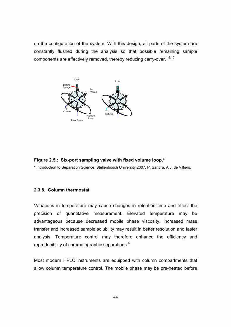
44

on the configuration of the system. With this design, all parts of the system are

constantly flushed during the analysis so that possible remaining sample

components are effectively removed, thereby reducing carry-over.1,6,10

ToWaste

Sample Loop

From Pump

ToColumn

SampleSyringe

LoadInject

ToColumn

Figure 2.5.: Six-port sampling valve with fixed volume loop.* * Introduction to Separation Science, Stellenbosch University 2007, P. Sandra, A.J. de Villiers.

2.3.8. Column thermostat

Variations in temperature may cause changes in retention time and affect the

precision of quantitative measurement. Elevated temperature may be

advantageous because decreased mobile phase viscosity, increased mass

transfer and increased sample solubility may result in better resolution and faster

analysis. Temperature control may therefore enhance the efficiency and

reproducibility of chromatographic separations.8

Most modern HPLC instruments are equipped with column compartments that

allow column temperature control. The mobile phase may be pre-heated before

45

entering the column. Temperatures may be regulated to a few tenths of a degree

from near-ambient to 200°C.1

2.3.9. Detectors

The ideal detector for liquid chromatography should be sensitive and selective

and characterized by a linear response to the solute over a wide dynamic range.

In addition the detector should be reliable with good stability and reproducibility,

non-destructive and have a small internal volume (to reduce extra-column band

broadening). To be compatible with modern high-efficiency, small-particle

columns, the detector should also have a fast response time.1

Liquid chromatographic detectors can be divided into two basic types. Bulk

property detectors respond to a mobile phase bulk property, such as refractive

index. In contrast, solute property detectors respond to a property of the solute,

such as UV absorbance or fluorescence. The bulk property detectors are

universal but are relatively insensitive compared to solute property detectors.

Pre- and post-column derivatization techniques may be used to expand the

applicability of the solute property detectors.6 The most common detectors used

in combination with liquid chromatography include.1

• Absorbance

• Fluorescence

• Electrochemical

• Refractive index

• Conductivity

• Mass spectrometry

• FT-IR

• Light scattering

46

The most common liquid chromatographic detectors in use are based upon UV-

visible absorption. These optical detectors are classified as fixed-wavelength,

variable wavelength or diode array detectors.6 For the purposes of this study,

diode array and mass spectrometric detectors will be discussed.

2.3.9.1. Diode array detector

Ultraviolet frequencies correspond to wavelengths of approximately 10 to 400 nm

while the visible spectrum extends from approximately 400 to 750 nm.11 UV-

visible energies correspond to electronic transitions, the energy needed to excite

an electron from one molecular orbital to the next.12 During transition to a higher

electronic level, a molecule can undergo simultaneous transitions between any of

a number of sub-levels, corresponding to various vibrational and rotational

states. As a result UV-visible absorption bands are broad and the corresponding

spectra are lacking in detail.13,14 Absorption by molecular oxygen limits the range

of conventional UV-visible detectors to wavelengths longer than approximately

190 nm.12

For absorbance measurements in the eluent from a chromatographic column, a

flow-through cell that is typically based on a Z-shaped design is used. In order to

minimize extra column band broadening, the volume of the cell is kept as small

as possible while at the same time maintaining a sufficient path length. Typical

cell volumes are of the order of 10 µL per centimeter of optical path length for

conventional diameter separation columns. The energy that passes through the

flow cell is compared with that of a reference and a signal that is the log of the

ratio of the two measurements is produced. In accordance with the Beer-Lambert

law, the absorption of monochromatic radiation is linear with solute

concentration.1,3

The Beer-Lambert law is typically given by the following equation:

47

A = log (I0 / I) = ε b c (10)

where I0 and I is the incident and transmitted intensities, ε is the molar

absorptivity of the solute with units of L.mol-1.cm-1, b the path length in

centimetres and c the molar concentration of the solute.1 This relationship

predicts that the magnitude of the absorption signal is proportional to the molar

absorptivity of the solute at the particular wavelength, the pathlength of the

detector and the solute concentration.

The most powerful ultraviolet-visible spectrophotometric detectors are diode

array instruments, which permit simultaneous collection of data over the

wavelength range of approximately 190 to 900 nm. These detectors are

equipped with an illumination source that is typically a combination of deuterium-

arc-discharge lamp for the UV radiation and a tungsten lamp for the visible

region. Diode array detectors work in a parallel configuration by simultaneously

monitoring all wavelengths. Energy from the sample cell is focused onto a

dispersion device, typically a grating, and the resulting monochromatic

wavelengths are directed onto the array of photodetectors (Figure 2.6.).

Complete spectra may thus be obtained in fractions of a second.3,6,15

Spectral data may be used to elucidate qualitative information from

chromatographic data in addition to the customary quantitative information. The

ratio of the absorbance at two wavelengths is structure specific and the purity of

a chromatographic peak may be elucidated by absorbance ratio-ing, a technique

whereby the ratio of absorbance at two wavelengths in the spectra is compared.

Analyte absorption spectra may also be compared with a library of user-

generated spectra for tentative compound identification.6

For UV detection, mobile phase solvents should be chosen to ensure low

absorbtion at the wavelength region of interest. Water, methanol and acetonitrile

48

permit operation in the UV range down to 210 nm. Where the acquisition

wavelengths are chosen so that the mobile phase does not absorb strongly, UV-

visible detectors can be used with gradient methods.6

Tungsten lamp

Deuterium lamp

Lens

Holmium oxide f ilter

CellProgrammable

slit Grating

1024 element

diode array

190 nm950 nm

Figure 2.6.: Components of a UV visible diode array detector.* * Agilent Technologies Inc., Waldbronn, Germany.

2.3.9.2. Mass spectrometric detector

Mass spectrometry, one of the most generally applicable of all analytical tools,

provides qualitative and quantitative information about the atomic and molecular

composition of inorganic and organic materials. The main advantages of mass

spectrometry as an analytical technique are increased sensitivity and specificity

compared to most other analytical techniques. The sensitivity and specificity

results primarily from a combination of the action of the analyzer as an effective

mass-to-charge ratio filter (thereby reducing background interference), sensitive

49

electron multiplier detectors and characteristic fragmentation patterns of solute

molecules.6 For these reasons, the mass spectrometer is probably the closest to

the ideal detector for liquid chromatography. Interfacing liquid chromatography

with mass spectrometry provides a powerful analytical technique particularly

amenable to trace level analysis. A schematic diagram of the components of a

typical liquid chromatography-mass spectrometry instrument is depicted in Figure

2.7.

Mass spectrometer Figure 2.7.: Components of an LC-MS system.2

A fundamental problem in coupling liquid chromatography with mass

spectrometry is the enormous mismatch between the relatively large mass flows

involved in HPLC and the vacuum requirements of the mass spectrometer.1 To

overcome this problem, several interfaces have been developed for efficient

sample introduction into the mass spectrometer.

HPLC

Ionizing interface

Focusing ion optics

Mass analyzer

Ion collection system

Data handling and system control

Vacuum system

50

Modern LC/MS systems generally utilize non-evacuated interfaces in which the

solvent is removed as the sample is ionized prior to introduction into the high-

vacuum environment of the mass spectrometer. Such interfaces mainly comprise

a combination of heaters, reduced pressure and gas nebulizers to volatilize and

remove unwanted eluent. Concurrent ionization of target compounds is achieved

by spraying the eluent either from an electrically charged capillary or across a

corona discharge needle during the final stages of evaporation. Generally the

configuration may be changed to produce positively or negatively charged ions.

The two prevalent types of atmospheric pressure interfaces that are also relevant

to the current study are the electrospray ionization (ESI) and atmospheric

pressure chemical ionization (APCI) interfaces. Each of these may fail to ionize

some types of compounds and switching between sources may be required in

order to ionize as many as possible of the sample components. Multimode

sources capable of ionizing diverse compounds are available but this design

suffers from a loss in sensitivity compared to dedicated sources.8

2.3.9.2.1. Electrospray interface

The electrospray ionization (ESI) interface (Figure 2.8.) is suited for use with

polar and ionized materials. It is a soft ionization technique that is characterized

by little fragmentation. It is also concentration independent and therefore suited

for use with microflow liquid chromatography systems.8

In the electrospray interface ionization is accomplished by passing the effluent

from the liquid chromatograph down a heated metal capillary tube along which a

3 to 4 kV electric charge differential is applied. This field charges the surface of

the liquid and forms a spray of charged droplets. The evaporating liquid is

sprayed out of the end of the tube where a concentric flow of an inert nebulizing

gas aids final evaporation. The charged droplets are attracted towards a capillary

sampling orifice while a counterflow of heated drying gas shrinks the droplets and

51

carries away uncharged material. The droplets shrink to the point where

electrostatic forces exceed the cohesive forces and the ions are desorbed into

the gas phase. The gas phase ions pass into the low-pressure region of the ion

source.3,8,16

Evaporation RayleighLimit

Reached

CoulombExplosion Analyte IonEvaporation

+

+++++ + +

++

++

-- -- -- +++++++

+++-- -

- --

++++

+++++++++++

-- -- --

+++++++++++

-- -- --

+++ +++----

+++ +++ ----

+++

++

+ ----

+++ +++ ----

+

++++

+ ----

+

++++

+ -- -- ++++ + +

++

-- -- -- ++++++

+++++

-- -- -- ++++++

+++++

-- -- --

+++

++

+----

++

++

+++

+ + + + + + + + + + + + +

+

+

Heated nitrogen dryinggas

Dielectric capillaryentrance

Nebulizer gas

Solvent spray

Electrospray Ions

Figure 2.8.: Electrospray interface and schematic ESI process.* * Agilent Technologies Inc., Waldbronn, Germany.

2.3.9.2.2. Atmospheric pressure chemical ionization interface

The atmospheric pressure chemical ionization (APCI) interface is typically used

for less polar compounds and can accommodate relatively large flow rates. As

with ESI, the design utilizes an off-axis flow path to ensure that only the charged

sample components enter the mass spectrometer while mobile phase solvent is

diverted out of the system. The APCI interface utilizes an inert nebulizing gas to

entrain and break up the eluent stream into small droplets. The nebulizer

capillary may be heated to aid evaporation of the solvent. After the desolvation

52

process, a dry vapor of solvent and analyte ions are produced which are sprayed

across a corona discharge needle operated at approximately 25 kV to ionize the

shrinking droplets. Solvent molecules are then ionized by the corona discharge

and act as an ionized reagent gas which subsequently ionizes analyte molecules

by atmospheric pressure chemical ionization. A cone-shaped impactor plate,

pointing towards the source region, is charged opposite to that applied to the

corona needle to draw the ions to the mass spectrometer entrance. A

countercurrent flow of dry nitrogen gas acts as a curtain to sweep uncharged

solvent vapors away from the pinhole orifice thus minimizing clustering of

charged analyte ions with water and other polar molecules.3,8 Figure 2.9.

presents a schematic representation of the APCI process.

Figure 2.9.: Atmospheric pressure chemical ionization interface and schematic APCI process.* * Agilent Technologies Inc., Waldbronn, Germany.

Dielectric capillary

Heater

HPLC inlet

Corona dischargeneedle

Vaporizer

Nebulizer gas

+

+

+

++

++

+

+

+

+

+

+

+

++

++

+

++

+

+

[Solv + H] + A -->Solv + [A + H]+

+ Dielectric capillary

Heater

HPLC outlet


Vaporizer

Nebulizer gas

+

+

+

++

++

+

+

+

+

+

+

+

++

++

+

++

+

+

[Solv + H] + A -->Solv + [A + H]+


Heater

HPLC


Vaporizer

Nebulizer gas


Heater

HPLC


Vaporizer

Nebulizer gas

+

+

+

++

++

+

+

+

+

+

+

+

++

++

+

++

+

+

[Solv + H] + A -->Solv + [A + H]+


Heater

HPLC inlet


Vaporizer

Nebulizer gas

+

+

+

++

++

+

+

+

+

+

+

+

++

++

+

++

+

+

[Solv + H] + A -->Solv + [A + H]+


Heater

HPLC inlet


Vaporizer

Nebulizer gas


Heater

HPLC inlet


Vaporizer

Nebulizer gas

+

+

+

++

++

+

+

+

+

+

+

+

++

++

+

++

+

+

[Solv + H] + A -->Solv + [A + H]+


Heater

HPLC outlet


Vaporizer

Nebulizer gas


Heater

HPLC outlet


Vaporizer

Nebulizer gas

+

+

+

++

++

+

+

+

+

+

+

+

++

++

+

++

+

+

[Solv + H] + A -->Solv + [A + H]+


Heater

HPLC


Vaporizer

Nebulizer gas


Heater

HPLC


Vaporizer

Nebulizer gas

+

+

+

++

++

+

+

+

+

+

+

+

++

++

+

++

+

+

[Solv + H] + A -->Solv + [A + H]+

+

53

2.3.9.3. Ion optics

Once a sample is ionized, the charged ions are moved from the interface through

a pinhole entrance into the higher-vacuum area of the spectrometer. An

oppositely charged draw-out lens works with movement from atmospheric

pressure to high-vacuum to pull ions into the entrance chamber. A repeller at the

back of the entrance has the same charge as the ions and forces them into the

focussing lens. Variable voltage charges on the focusing lens with the same

polarity as the molecular ions function by squeezing the ions into a narrow

stream that is focussed on the mass analyzer.

2.3.9.4. Mass analyzer

Functionally, all mass spectrometers perform three basic tasks; creating gaseous

ion fragments from the sample, sorting these ions according to their mass-to-

charge (m/z) ratios and measuring the relative abundance of the ion fragments of

each mass.6 LC-MS systems may be categorized into four basic designs

according to the mass analyzer system used. The quadrupole (or octapole) type

analyzer use a bundle of oppositely charged rods, swept with radio frequency, to

separate and focus the ions on the detector. In the ion trap design, a three

dimensional spherical or quadrupole arrangement is used to contain and then

release the ions. Separation is achieved by varying the dc/RF voltage to expel

ions of increasing m/z into the detector. The third type ejects ions in a burst mode

into a time-of-flight tube where the traveling time to the detector is dependent on

the m/z ratio of the ions, with lighter fragments arriving at the detector first. The

fourth type has a trapping volume that is bombarded with a full frequency radio

signal that momentarily promotes ions to a higher-energy state. Upon collapse a

modified all-frequency signal is produced which is analyzed with Fourier

transform software to produce an intensity versus m/z ratio signal.8

54

Combinations of one or all of these designs are used to create hybrid systems

that combine multiple mass analyzer modules with collision and ion-trapping cells

to separate, fragment and detect not only the molecular ion, but also fragments,

commonly referred to as daughter ions. The ability of these tandem MS or

MS/MS systems to determine fragmentation products of particular molecular ions

in this manner allows the analyst to perform structural elucidation studies or to

confirm the identity of the solute. Hybrid systems are also suited for accurate

quantitation at trace levels as the analyzers can be tuned to single ion

frequencies corresponding to the molecular ion and daughter ion of the target

compound, thus generating very specific signals with low background noise.8 The

focus of the following discussion will be on the triple quadrupole mass

spectrometer design, utilized in this study.

2.3.9.4.1. Triple quadrupole mass analyzers

The triple quadrupole mass spectrometer combines two conventional scanning

quadrupole analyzers with a collision cell. The target ion selected from the first

analyzer is allowed to collide with inert gas molecules in the collision cell to

induce fragmentation. The fragmented ions are then passed into the second

analyzer for separation and subsequent detection. In earlier models, a

quadrupole was used as a collision cell hence the term triple quadrupole mass

spectrometer.8 To identify these components in the following discussion, the first

quadrupole analyzer, collision cell and second quadrupole analyzer will be

numbered Q1, Q2 and Q3, respectively.

The quadrupole analyzer has four cylindrical rods clamped in a tubular

arrangement by ceramic collars. The exact hyperbolic spacing between

diagonally opposed rods is critical for mass spectrometer operation. Opposing

rods have the same direct current charge applied to them while adjacent rods

have opposite charge applied. Ions are focussed into the tunnel formed by the

55

four rods and follow a corkscrew flight path down the rods as they are swept

forward by a changing radio frequency signal. Only ions following stable

trajectories at a given frequency are expelled from the quadrupole to collide with

the ion detector. Ion masses that follow unstable paths at the particular dc/RF

voltage collide with the inner walls of the analyzer rods, and are not detected.8

Two scanning techniques, continuous scanning and selected ion monitoring

(SIM) are used to acquire mass spectrometric data. In the continuous scan

mode, a scan of a pre-defined mass range is performed at fixed time intervals for

the duration of the experiment. A total ion current profile may thus be generated

that represents a normalized plot of the sum of ion abundance as a function of

time. Mass spectra may then be obtained for each of the sequence of scans thus

performed. When operated in SIM mode, one or a few ions may be monitored

exclusively throughout the experiment.3

Following ionization and ion focusing, ions enter Q1, where the direct-current

charged surfaces of the analyzer are then swept with a changing radio frequency

signal that selects different mass ions for each frequency and allows them to

follow a stable path through the analyzer. The stable ions at each frequency are

then expelled into the collision cell Q2. Here, selected parent ions are

fragmented by collision with molecules of an inert gas. The energy of these

collisions, and therefore the degree of fragmentation that the molecules undergo,

is regulated by the collision voltage. The resulting daughter ions are then

focussed onto the second quadrupole analyzer, Q3. The mass spectrum of the

resulting daughter ions is obtained by scanning with quadrupole analyzer Q3. In

this manner a complete three-dimensional fragmentation map may be obtained

by recording the mass spectrum of each fragmentation ion of a parent

compound.8

The triple quadrupole LC-MS may be operated in any one of four modes

depending on the aim of the experiment. In the parent ion mode, Q1 is scanned

56

and all ions sent to the fragmentation chamber. Quadrupole Q3 is then ‘parked’

at a frequency to select a specific fragment ion common to related compounds.

In the daughter ion mode, Q1 is fixed at a suitable frequency to select a specific

ion that is passed to the collision cell. Quadrupole Q3 is then scanned for

fragmentation information that can be used to identify the structure of the ion

under investigation. In the neutral loss mode, both Q1 and Q3 are scanned with a

specific frequency offset. Only ions that loose a common uncharged fragment are

detected, thereby providing information about their fragmentation type. The fourth

operational mode is particularly suited for the trace analysis of compounds in

complex mixtures, even in cases where the components are not completely

separated. In this mode, both Q1 and Q3 are set at single ion frequencies

specific for the compound (ion) under investigation and one of its daughter

fragments, respectively. The signals that are generated are therefore very

specific to the compound under investigation while interferences are excluded.

By using a small scan range and a high signal sampling rate, a greater number of

data points may be averaged for a given m/z value and time, thus producing a

signal with higher signal-to-noise ratios. In this way sensitivity and detection limits

may be optimised.8,18

2.3.9.5. Ion detectors

The resolved ion beam, after passage through the mass analyzer, sequentially

strikes the ion detector. Several types of detector are used with mass

spectrometers. For ion currents less than 10-15 A, an electron multiplier detector

is required.6 This discussion will focus on the electron multiplier detector.

The electron multiplier detector uses an impact and cascade mechanism. When

a charged particle strikes the membrane surface of the conversion dynode, the

impinging ions are converted to electrons. The resulting electrons then strike the

coated surface of the detector wall, releasing multiple electrons. These electrons

57

in turn cascade down the curved tube of the detector, releasing multiple electrons

on each impact. This cascade of electrons amplifies the signal of a single contact

for transfer to the data system. Gain ranges of the order of 105 to 107 may be

attained with this detector design.6,8,17

2.3.9.6. Vacuum system

The operation of the spectrometer requires a collision-free path for the ions. To

achieve this, the pressure in the spectrometer should be less than 10–6 torr to

prevent collisions of the ions with air molecules.6,8

The required high-vacuum environment is established in a two-staged process. A

rough vacuum is established first with a laboratory rotary-vane oil pump. A

turbomolecular pump connected in series provides the final operating vacuum.

The turbo pump has a series of vanes mounted on a shaft that rotates at very

high speeds. The vanes force the air from the vacuum chamber prior to venting it

out through the roughing pump. The turbo pump contains no oil that can

contaminate the analyzer, but may be prone to mechanical failure.8

2.3.9.7. LC-MS data handling

The data system may be used to record the signal strength of all ions detected

as well as spectral information at any given time in the chromatographic run in a

three dimensional block of data. A total ion chromatogram (TIC) is a plot of the

signal strength of all ions versus time whereas a spectrum is a plot of signal

strength versus mass to charge ratio at any given time. The m/z ratios of the ions

are determined by calibrating the dc/RF frequency with standards of known mass

to charge ratio.8

58

2.4. Gas chromatography

Gas chromatography is in many instances the technique of choice for the

separation of thermally stable and volatile organic and inorganic compounds. In

gas chromatography, the sample, often vaporized, is injected onto the head of a

chromatographic column. As with HPLC, the column is where the actual

separation of sample components occurs. Elution is brought about by the flow of

an inert gaseous mobile phase. The mobile phase transports the gaseous

analyte through the column and separation, specific to the column and analyte

combination, occurs prior to their detection. Gas-liquid chromatography, based

upon the partitioning of the analyte between a gaseous mobile phase and a liquid

stationary phase which is immobilized on the surface of an inert solid, is by far

the most widely used form of gas chromatography.1,6 This discussion will focus

exclusively on gas-liquid chromatography. An overview of relevant gas

chromatographic techniques and hardware is presented with special reference to

the equipment utilized in publications referenced in this study.

2.4.1. Gas chromatographic columns

Two general types of columns are encountered in gas chromatography, namely

packed and capillary columns. Capillary columns provide faster and more

efficient separation and are almost exclusively used today. Capillary columns are

usually constructed of fused silica and may be as long as 50 m or more. The high

permeability or low resistance to carrier-gas flow of capillary columns enables

long columns to generate large numbers of theoretical plates.2,6 In order to fit into

an oven for thermostatting, capillary columns are formed into coils of suitable

diameter.

59

In capillary columns the stationary phase is a uniform film of liquid with thickness

of the order of a few tenths of a micrometer coated on the interior of the capillary.

Film thickness primarily affects the retentive character and capacity of a column.

Desirable properties for the immobilized liquid stationary phase includes low

volatility, thermal stability, chemical inertness and solvent characteristics such

that k’ and α values for the solutes to be resolved fall within a suitable range. The

criteria for column efficiency, described earlier for HPLC, are fully applicable to

gas chromatography. Two differences should be noted however. First, there is no

contribution to band broadening due to eddy diffusion in capillary columns.

Second, longitudinal diffusion is more important in gas chromatography as

diffusion rates in gasses are much larger than that in liquids.1

Retention time for a solute in a given column depends upon its distribution

constant, as discussed earlier. In GC this distribution is dependant on the

volatility of the analyte, and therefore the temperature, as well as on chemical

interaction with the stationary phase. Two types of separation can be

distinguished. In the first instance, when an apolar stationary phase such as

polydimethylsiloxane (PDMS) is used, non-specific interaction with the stationary

phase dominates. Analytes are therefore separated largely due to differences in

volatility. This is determined by the respective vapor pressures of the analytes,

and this mode of separation is referred to as a boiling point separation (analytes

elute in order of increasing boiling points). In contrast, when more polar

stationary phases such as polyethylene glycol (PEG) are used, specific chemical

interactions such as dipole interactions and hydrogen bonding predominantly

determine analyte retention. A range of stationary phases, varying from relatively

apolar to relatively polar, are available to achieve satisfactory separations.1

60

2.4.2. Carrier gases

Chemically inert carrier gases that are most often used in gas chromatography

include helium, nitrogen and hydrogen. Associated with the gas supply are

pressure regulators and gauges and optional purifiers to remove impurities and

moisture. Flow rates are controlled by pressure regulators in the instrument.

Modern gas chromatographs are often equipped with electronic flow meters that

enable constant flow or constant pressure modes of operation.1

The purpose of the carrier gas is to transport the sample through the column to

the detector. The three most common gases provide practically the same

minimum plate height, but the optimal linear velocities increase in the order

nitrogen < helium < hydrogen. Plate height curves for helium and hydrogen are

flatter meaning that a smaller loss in efficiency will be suffered when linear

velocities higher than the optimum are used, leading to significant reductions in

analysis times. The ratio of carrier gas viscosity to the diffusion coefficients of the

sample components should be as small as possible and in this respect hydrogen,

followed by helium are the most efficient carrier gasses.6

2.4.3. Sample injection systems

In order to effectively exploit the high efficiencies of GC columns, it is required

that a suitable sample size be introduced as a discrete band of vapor. The most

common method of sample injection involves the use of a microsyringe to inject a

liquid or gaseous sample through a self-sealing septum into a vaporizer port,

located at the head of the column. The injection port is usually maintained at

about 50°C above the boiling point of the least volatile component of the sample.

Capillary columns, commonly used today, require smaller sample sizes than that

produced by a microsyringe. A split injector is employed to deliver a fraction of

the injected sample to the head of the column, with the remainder going to waste.

61

Splitless injection may be utilized for trace-level analysis where the entire

sample, including any solvent, is injected onto the column (this method often

requires focusing mechanisms to avoid excessive band broadening due to

injection). The injection port is vented after a predetermined amount of time to

eliminate excess solvent from the system. Alternatively, although less often used,

more reproducible injection of liquids and gases may be achieved by using a six-

port rotary sample valve, similar to that used with liquid chromatography.1,6

Headspace sampling is a technique that may be utilized when only the vapor

above the sample is of interest, particularly if the sample is a liquid that would

normally require some processing before injection, such as blood. Headspace

sampling can be done on any sample provided that the partition coefficient allows

a sufficient amount of analyte into the gaseous phase.6

Purge and trap may similarly be used to purge volatile organic constituents from

a sample which may then be trapped on a suitable adsorbent. Efficient

desorption may be achieved by purging with an inert gas at elevated temperature

(~300°C). Desorbed volatiles are typically re-focused by cryo-trapping. The gas

chromatographic separation may then proceed upon heating and elution of the

volatiles onto the chromatographic column.6

Gas-liquid chromatography reaches a practical limit when the amount of energy

needed to vaporize the sample is the same as the amount of energy required to

break a carbon-carbon bond. The technique of pyrolysis (or controlled

fragmentation) extends gas chromatographic analysis to such low-volatility

compounds as rubber and polymers and involves the formation of volatile

fragments for subsequent introduction into the chromatographic column for

analysis.6

Cool on-column injection is a capillary column inlet that allows direct deposition

of liquid sample into the column. Both the inlet and the column are held

62

substantially below the boiling point of the solvent during the injection, after which

both are increased to vaporize the sample and initiate chromatography. The

temperature of the inlet should be controlled independently from the column

temperature for highest reproducibility and flexibility. Since the sample is

deposited directly into the column without being evaporated first, cool on-column

inlets have the highest reproducibility and lowest discrimination and

decomposition of any inlet. Sample introduction into small diameter capillary

columns may however be problematic, and focusing methods generally are

imperative in this mode of injection.2

Solid Phase Microextraction (SPME) is a form of sample preparation which

involves exposing a polymer-coated fused silica fiber to a sample. The analytes

partition into the stationary phase until an equilibrium has been reached, after

which the fiber is removed from the sample. Analytes may then be thermally

desorbed in the injector of a gas chromatograph. The fiber is typically contained

in a syringe-like device to facilitate handling. SPME sampling may be performed

directly in liquid samples or, if the analytes are sufficiently volatile, from the

headspace above the liquid sample. In SPME analytes are not extracted

quantitatively from the matrix, instead the extracted quantity depends on the

equilibrium distribution of analyte between the sorbent and sample matrix. This

approach requires careful calibration utilizing surrogates or standard addition to

quantify the analytes and to compensate for matrix variations and the associated

effects on distribution ratios.19

Automatic samplers may be utilized to provide unattended operation of most

sample introduction techniques. Automatic samplers are consistently more

precise than manual sample measurement and injection.6

63

2.4.4. Derivativization

Derivatization prior to gas chromatographic analysis is often desirable to improve

thermal stability, adjust volatility or to introduce a detector-orientated tag into a

molecule. Ideally all relevant functional groups should be derivatized

quantitatively and rapidly and upon injection of the reaction mixture, the excess

reagent should elute with the solvent peak.6

2.4.5. Column oven

Column temperature is an important variable, as outlined above, and must be

controlled to a few tenths of a degree for precise GC work. The optimal column

temperature depends on the boiling point range of the sample components and

degree of separation required. In general, optimal resolution is associated with

minimal temperature, but the cost of lower temperature is an increase in elution

time.1 Most often temperature gradients are used in capillary GC to effectively

separate analytes across a broad range of boiling points with sufficient resolution

in an acceptable time.

2.4.6. Detectors

As is the case with HPLC, a multitude of detectors have been developed for gas

chromatography. The characteristics of the ideal detector are basically the same

as that described for HPLC. Detectors available for use with gas

chromatographic systems include the following:1

• Flame ionization detector

• Thermal conductivity detector

• Sulfur chemiluminescence detector

64

• Electron-capture detector

• Atomic emission detector

• Nitrogen phosphorous detector

• Flame photometric detector

• Mass spectrometric detector

• Infrared spectrophotometric detector

The flame ionization detector (FID) is the most widely used and generally

applicable detector for gas chromatography. Selective detectors such as the

electron-capture detector (ECD), flame photometric detector (FPD) and nitrogen-

phosphorus detector (NPD) are primarily responsive to specific functional groups.

These detectors have found specialized areas of application such as the analysis

of environmental samples for pesticides and other pollutants. Spectral detectors

such as MS and IR not only serve as sensitive and selective detectors, but also

to identify compounds.1

For the purposes of this study, the discussion will be limited to detectors that

were used to measure the substances under investigation, as described in the

literature references, namely the nitrogen-phosphorus detector (NPD) and mass

spectrometric (MS) detector. As the principles of the mass separation and ion

detection were discussed earlier and apply similarly to GC-MS, the focus here

will be limited to ionization for GC-MS.

The nitrogen-phosphorus detector is primarily responsive towards compounds

containing nitrogen and phosphorus. The effluent from the gas chromatograph is

passed into the detector where a dilute hydrogen and air gas mixture is heated to

yield reactive hydrogen atoms. The hydrogen atoms, through a series of chain

reactions, produce a highly reactive chemical environment that primarily exists in

a gaseous layer near the hot thermionic source. Analyte molecules are

decomposed in the hot, chemically active layer and nitrogen or phosphorus

65

compounds, which form electronegative decomposition products, are selectively

ionized. The resulting ion current is then measured at the collector electrode.2

Gas chromatography may be coupled to mass spectrometry to provide a

powerful tool for quantitative and qualitative analysis of complex sample

mixtures. The flow rates employed for capillary columns are generally low

enough that the column output may be fed directly into the ionization chamber of

the mass spectrometer.

Electron impact ionization may be utilized to ionize solutes eluting from the gas

chromatograph in a high vacuum. In electron impact ionization, the analyte

molecules are bombarded with electrons in the heated ionization source. The

energy of the ionizing electrons is typically regulated to a value of 70 eV by

controlling the accelerating voltage, established between the cathode and source

housing. When an electron strikes a neutral molecule, it may ionize the molecule

by knocking out an additional electron to create a radical cation. In addition to

ionization, electron impact ionization may also fragment a molecule to yield a

characteristic mixture of ions. Under electron impact conditions the molecular ion

is often unstable resulting in the loss of useful information concerning the

molecular weight of the analyte.1,3,12

Chemical ionization is effected by reacting neutral analyte molecules with a high

concentration of reagent gas ions. An electron beam mainly ionizes the reagent

gas molecules as these exceed the concentration of the analyte molecules by

several orders of magnitude. The source is operated at high pressure compared

to electron impact ionization with the result that ion-molecule interactions

predominate. Chemical ionization is generally less energetic than electron impact

ionization resulting in the production of stable molecular ions or molecular ion

adducts with little additional fragmentation. The high pressure environment in the

chemical ionization source also favor the production of thermal electrons which

66

may be captured by molecules with a high electron affinity thus producing

negatively charged molecular ions.3

67

REFERENCES

(1) D. A. Skoog, F. J. Holler, T. A. Nieman, PRINCIPLES OF

INSTRUMENTAL ANALYSIS, 5th ed. (1998), Saunders College

Publishing, Philadelphia, 673 - 777.

(2) R. L. Grob, MODERN PRACTICE OF GAS CHROMATOGRAPHY, 3rd

ed.(1995), John Wiley & Sons, 605 Third Avenue, New York, NY 10158-

0012,.

(3) C. F. Poole, S. K. Poole, CHROMATOGRAPHY TODAY, (1991), Elsevier

Science Publishing Company Inc., 655 Avenue of the Americas, New

York, NY 10010, U.S.A.

(4) P. Sandra, RESOLUTION – DEFINITION AND NOMENCLATURE,

Journal of High Resolution Chromatography, 12 (1989), 82 - 86.

(5) P. Sandra, RESOLUTION – COLUMN EFFICIENCY, Journal of High

Resolution Chromatography, 12 (1989), 273 - 277.

(6) H. H. Willard, L. L. Merritt Jr., J. A. Dean, F. A. Settle Jr.,

INSTRUMENTAL METHODS OF ANALYSIS, 7th ed. (1988), Wadsworth

Publishing Company, Belmont, California, 465 - 652.

(7) T. Welsch, D. Michalke, (MICELLAR) ELECTROKINETIC

CHROMATOGRAPHY:AN INTERESTING SOLUTION FOR THE LIQUID

PHASE SEPARATION DILEMMA, J. Chromatogr., A, 1000 (2003), 935 - 951.

(8) M. C. McMaster, LC/MS A PRACTICAL USER’S GUIDE, (2005), John

Wiley & Sons Inc., 111 River Street, Hoboken, NJ 07030, 51 - 84.

(9) J. Cazes, ENCYCLOPEDIA OF CHROMATOGRAPHY, 2nd ed.(2005),

Taylor and Francis Group, 6000 Broken Sound Parkway, NW, Suite 300,

Boca Raton, FL 33487-2742, 1473 - 1476.

(10) HPLC FOR ENVIRONMENTAL ANALYSIS, Hewlett-Packard Company,

Publication Number: 12-5091-9750E, Printed in France 05/94.

(11) D. D. Ebbing, S. D. Gammon, GENERAL CHEMISTRY, 6th ed. (1999),

Houghton Mifflin Company, 222 Berkeley Street, Boston MA, 279.

68

(12) L.G. Wade Jr., ORGANIC CHEMISTRY, 4th ed.(1999), Prentice-Hall inc.,

Upper Saddle River, New Jersey 07458, 856 - 858.

(13) R. T. Morrison, R. N. Boyd, ORGANIC CHEMISTRY, 6th ed.(1992),

Prentice-Hall inc., Englewood Cliffs, New Jersey, 07632, 597.

(14) D. L. Pavia, G. M. Lampman, G. S.Kriz, INTRODUCTION TO

SPECTROSCOPY, Harcourt Brace Publishers, 1996, 267-302.

(15) REFERENCE MANUAL: AGILENT 1100 SERIES DIODE ARRAY AND

MULTIPLE WAVELENGTH DETECTORS, Manual Part Number: G1315-

90005, Edition 05/2004, Agilent Technologies Inc., Hewlett-Packard-

Strasse 8, 76337, Waldbronn, Germany.

(16) BASICS OF LC/MS, Hewlett-Packard Company, (23) 5968-2543E, Printed

in the U.S.A., 10/98.

(17) J. Baker, MASS SPECTROMETRY, 2nd ed.(1999), John Wiley and Sons,

95 - 116.

(18) WATERS MICROMASS QUATTRO PREMIER XE MASS

SPECTROMETER OPERATOR’S GUIDE, Waters Corporation, 34 Maple

street, MA 01757, U.S.A.

(19) A. J. Handley, EXTRACTION METHODS IN ORGANIC ANALYSIS,

(1999), Sheffield Academic Press Ltd, Mansion House, 19 Kingfield Road,

Sheffield S11 9AS, England.

69

CHAPTER 3

Development and optimization of a sample preparation procedure for the liquid chromatographic analysis of

trace levels of 3-alkyl-2-methoxypyrazines in wine

3.1. Introduction

The concentrations of 3-alkyl-2-methoxypyrazines in South African Sauvignon

blanc wine are expected to fluctuate between approximately < 0.1 and 14 ng/L.1

It is essential that the method of analysis utilized is capable of precise

measurements in the range of typical values. For the application of compiling a

profile of relative abundances of 3-alkyl-2-methoxypyrazines in South African

Sauvignon blanc wine, the method should preferably yield detection limits of the

order of 0.005 ng/L or better. The ultra-low levels expected for the analytes under

investigation necessitate highly sensitive and selective extraction and analysis

methods for quantitative purposes. To facilitate the successful liquid

chromatography-mass spectrometric (LC-MS) analysis of sub parts-per-trillion

levels of 3-alkyl-2-methoxypyrazines in Sauvignon blanc wine, an efficient and

compatible sample clean-up and pre-concentration procedure therefore needs to

be developed and optimized.

A preliminary investigation revealed that an estimated detection limit in the order

of 1 pg of IBMP may be expected from some modern LC-MS systems. It then

follows that if the equivalent of 200 mL of wine can be loaded on the column, a

limit of detection of 0.005 ng/L of IBMP may be achieved. A sample pre-

concentration step is therefore essential in order to achieve the required

sensitivity. Analytical liquid chromatographic systems offer injection volumes of

up to 1 mL, but large injection volumes may overload the analytical column and

70

degrade sensitivity and precision, depending on the matrix of the extract.

Utilization of large injection volumes (in the order of 1 mL) may therefore be

feasible, provided that the extract can be chromatographed without loss of

resolution. It is therefore essential that the pre-concentration procedure is

selective so that the bulk of the wine matrix components may effectively be

eliminated to yield relatively clean, aqueous extracts. The ideal sample

preparation procedure should therefore affect pre-concentration of a factor of at

least 200 as well as a measure of selectivity for sample clean-up to facilitate

large injection volumes, in order to impart the desired sensitivity to the method.

The sample preparation procedure should also be robust and impart a relatively

small amount of quantitative uncertainty to the method.

The efficiency of solvent extraction, solid phase extraction (SPE) and stir bar

sorptive extraction (SBSE) sample preparation techniques were evaluated to

determine their suitability for the application. The preliminary experimental work

was performed utilizing wine fortified with mg/L quantities of 3-isobutyl-2-

methoxypyrazine and measuring the residues with reversed phase liquid

chromatography with UV detection. Subsequent experiments, aimed at

evaluating the efficiency of the said techniques for the extraction of 3-alkyl-2-

methoxypyrazines from the distillates of wine samples, were performed with the

LC-MS method utilizing APCI ionization. Where LC-MS was used for measuring

the residues, samples were fortified at ng/L levels.

Solvent extraction is a separation method based upon the distribution of a solute

between two immiscible liquids. The distribution coefficient of the solute in the

two liquids is the equilibrium constant that describes the distribution ratio of the

solute between the two phases. Generally, distribution coefficients between two

immiscible liquids is sufficiently large to accomplish efficient partitioning of the

solute into one or the other liquid.2

71

Solid phase extraction (SPE) is a versatile sample preparation technique utilizing

a multitude of adsorbents based on polar, hydrophobic and/or ion exchange

interactions.3 Adsorbent chemistries and parameters for separation are based on

the same principles that apply to equivalent liquid chromatographic techniques.

Adsorbent material is typically packed in disposable cartridges for convenient

application of liquid samples. SPE may be used to establish three important pre-

requisites for trace-level analysis namely enrichment, removal of interfering

matrix components and changing of the sample matrix for subsequent analyses.

Since the analyte can either be adsorbed on the SPE phase or flow through

unretained, two general separation strategies are possible. In the first case, the

liquid sample may be forced through the conditioned cartridge where the analyte

is retained on the phase. The matrix may then be washed off followed by

selective elution of the analyte. Alternatively, the conditioned phase may retain

interferents while the analyte pass through the column, allowing purification of

the sample solution. SPE also offer advantages over conventional liquid-liquid

extraction such as enhanced selectivity, speed, broad application range, low

solvent consumption and potential automation.

Distillation permits a simple and convenient method for separation of volatile

components from a sample mixture. As distillation was also used successfully as

part of sample preparation procedures in several publications referenced in this

study, the effectiveness thereof was evaluated for sample clean-up and pre-

concentration.4,5,6

Stir bar sorptive extraction (SBSE) is a new solventless extraction method where

the analyte are enriched from the sample matrix by sorption into a

polydimethylsiloxane (PDMS)–coated stir bar.7 Extraction of the analyte may be

achieved by stirring directly in liquid samples or alternatively, by placing the bar

in the headspace of the agitated or heated sample. Partitioning of the analyte

between the PDMS phase and the sample matrix is based on the relevant

equilibrium distribution ratio as well as the ratio of phases present. Analysis may

72

be performed following thermal desorption (for gas chromatographic analysis), or

alternatively liquid desorption may be achieved by stirring with a small volume of

suitable solvent for subsequent liquid phase separation.8

This Chapter reports the evaluation of each of the outlined techniques as well as

combinations thereof, for sample preparation in the trace level determination of

3-alkyl-2-methoxypyrazines in wine.

3.2. Experimental

3.2.1. Materials

High purity solvents and chemicals were used throughout the experiment.

Dichloromethane (DCM) and tannic acid were from Merck (Darmstadt,

Germany), Di-ethyl ether from Saarchem (Merck, South Africa), IBMP,

acetonitrile, ethanol and methanol from Aldrich (Sigma-Aldrich, South Africa)

hexane from Burdick & Jackson (Honeywell International, U.S.A.), formic acid

from Associated Chemical Enterprises (ACE, South Africa) and sodium

hydroxide from Sigma (Sigma-Aldrich, South Africa).

Standards were prepared by weighing appropriate amounts of reference material

on an analytical balance. Dilutions were made using A-grade volumetric

glassware. Intermediate standards were prepared in ethanol while working

standards were prepared in 10% ethanol. Wine samples were fortified

volumetrically by adding appropriate amounts of standards.

The SPE products that were evaluated were as follows (Table 3.1.):

73

Table 3.1.: SPE products evaluated in the investigation.

Manufacturer International Sorbent Technologies Ltd 9 Description IST Isolute C18(EC) Sorbent chemistry Octadecyl Sorbent mass 200 mg / 3 mL Particle size 50 µm Endcapped yes Manufacturer Waters Corporation 10 Description Oasis HLB Sorbent chemistry Divinylbenzene and N-vinylpyrrolidone Sorbent mass 60 mg / 3 mL Particle size 30 µm Manufacturer Waters Corporation 10 Description Oasis HLB Sorbent chemistry Divinylbenzene and N-vinylpyrrolidone Sorbent mass 500 mg / 6 mL Particle size 30 µm Manufacturer Phenomenex 11 Description Strata SDB-L Sorbent chemistry Unmodified polystyrene-divinylbenzene Sorbent mass 500 mg / 3 mL Particle size 100 µm Manufacturer Waters Corporation 10 Description Waters Sep-Pac Vac Silica Sorbent chemistry Silica Sorbent mass 200 mg / 3 mL Manufacturer Phenomenex 11 Description Strata SCX Sorbent chemistry Silica based sulfonic acid Sorbent mass 500 mg / 3 mL Particle size 55 µm

74

3.2.2. Liquid chromatographic methods and instrumentation

An Agilent 1100 LC system (Agilent Technologies, Waldbronn, Germany) fitted

with quaternary pump, autosampler, column oven and UV-visible diode array

detector (DAD) was used to analyze the fortified wine samples, distillates and

extracts. The liquid chromatographic parameters were as follows: The mobile

phase was an acetonitrile/water gradient starting at 50% acetonitrile for 30

seconds, then increasing acetonitrile to 95% in 7 minutes, followed by 95%

acetonitrile for 4 minutes, at a flow rate of 0.5 mL/minute. The column was a

Phenomenex Luna C18, 150 x 4.6 mm, with 3 µm particle-size, thermostatted at

30°C. Variable injection volumes were used. The chromatographic signal at 292

nm was acquired while spectra between 190 and 400 nm were recorded.

Where the residues were measured with LC-MS, a Waters Alliance LC system

(Waters Corporation, Milford, U.S.A.) incorporating a quaternary pump,

autosampler, column oven and Micromass Quattro Premier XE tandem

quadrupole mass spectrometric detector (Manchester, U.K.), was used.

Ionization was achieved utilizing a dedicated APCI probe. The column was a

Phenomenex Luna C18 of dimensions 250 x 4.6 mm x 3 µm, thermostatted at

40°C. The mobile phase was a methanol/water gradient, starting at 95% water

for 1 minute, then changing to 95% methanol in 18 minutes, followed by 3

minutes at 95% methanol. A variable flow-rate was used, starting at 0.75

mL/minute for 1 minute and then changing with the solvent gradient to 0.85

mL/minute in 18 minutes. Re-equilibration time was 4 minutes, during which the

flow also reverted to the starting value of 0.75 mL/minute. Data acquisition was in

MRM mode, acquiring data for the relevant primary as well as secondary ion

transitions (167 > 125, 167 > 124). The mass spectrometer source parameters

were as in Table 3.2.:

75

Table 3.2.: Source parameters for Ion Sabre APCI probe.

Parameter Value Corona needle 4.4 µA Cone voltage 34 V Extractor voltage 6 V RF lens 0 V Source temperature 150°C Desolvation temperature 250°C Cone gas (N2) 100 L/Hr Desolvation gas (N2) 200 L/Hr

3.3. Results and discussion

3.3.1. HPLC method performance

The UV spectrum of IBMP, as measured with the DAD detector, revealed two

maxima, at 214 nm and 292 nm, respectively (Figure 3.1.). Despite the fact that

the absorption at 214 nm is more intense, the 292 nm wavelength was used for

quantitation as less possible interference from the wine matrix components were

anticipated at the longer wavelengths.

76

Using a detection wavelength of 292 nm, the HPLC method provided adequate

selectivity for the detection of IBMP, fortified to mg/L levels, in the presence of

wine matrix components (Figure 3.2.).

nm200 225 250 275 300 325 350 375

mAU

0

1

2

3

4

5

6

7

nm200 225 250 275 300 325 350 375

mAU

0

1

2

3

4

5

6

7

Figure 3.1.: UV spectrum of 3-isobutyl-2-methoxypyrazine, acquired by HPLC-DAD (10 ng in mobile phase).

77

Figure 3.2.: Comparison between chromatograms obtained for a Sauvignon Blanc wine (bottom), and the same wine spiked with 3.0 mg/L of 3-isobutyl-2-methoxypyrazine (top). Injection volume: 10 µL, detection: 292 nm. Other HPLC conditions are as specified in section 3.2.2.

The linear response of the system over the concentration range used during

method development was determined by injecting various masses of IBMP. The

response of the system was found to be linear over the entire mass range used

(Figure 3.3., r = 0.9999). The limit of detection (LOD) was estimated

conservatively using a signal-to-noise (S/N) ratio of more than 10, providing a

value of 0.50 ng injected on-column. The LOD was determined using a standard

solution and therefore does not necessarily apply to real wine extracts.

min0 2 4 6 8 10 12 14

mAU

0

10

20

30

40

50

60

70

IBMP

min0 2 4 6 8 10 12 14

mAU

0

10

20

30

40

50

60

70

IBMP

78

0

50

100

150

200

250

300

0 20 40 60 80 100 120

Mass IBMP (ng)

Peak

are

a (m

AU

)

Figure 3.3.: Calibration curve for the HPLC-UV analysis of IBMP standard, 0.50 to 100 ng, r = 0.9999.

The precision of the liquid chromatographic system was evaluated by performing

repeated injections of 25 μL of a standard solution containing 2.5 mg/L IBMP.

Repeatability, as expressed by the relative standard deviation (RSD) of the peak

area, was found to be excellent (0.7% RSD).

3.3.2. Development and optimization of a solvent extraction procedure

3.3.2.1. Comparison of different solvents

It is essential that the analytes of interest display a favorable distribution between

the extraction solvent and the sample matrix to ensure their efficient extractive

separation from the wine matrix. Several solvents have been used for the

extraction of methoxypyrazines from wines. Kotseridis et al.12 used a di-ethyl

ether/hexane mixture for the extraction of various compounds including IBMP,

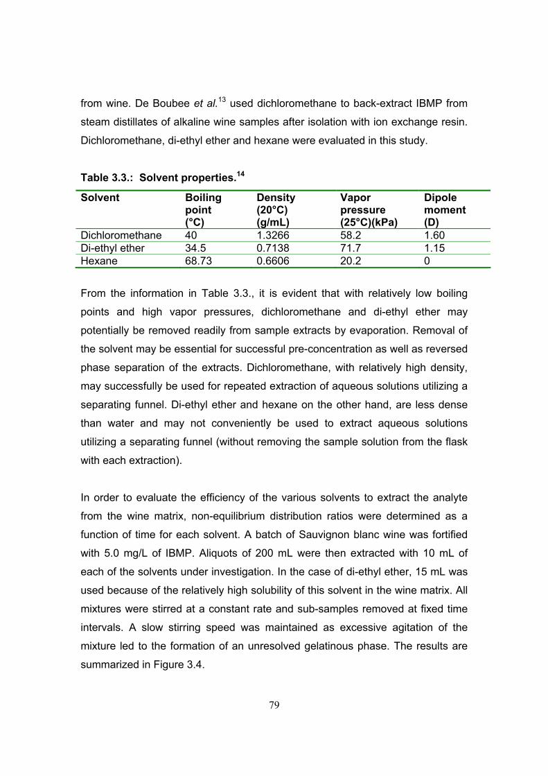
79

from wine. De Boubee et al.13 used dichloromethane to back-extract IBMP from

steam distillates of alkaline wine samples after isolation with ion exchange resin.

Dichloromethane, di-ethyl ether and hexane were evaluated in this study.

Table 3.3.: Solvent properties.14

Solvent Boiling point (°C)

Density (20°C) (g/mL)

Vapor pressure (25°C)(kPa)

Dipole moment (D)

Dichloromethane 40 1.3266 58.2 1.60 Di-ethyl ether 34.5 0.7138 71.7 1.15 Hexane 68.73 0.6606 20.2 0

From the information in Table 3.3., it is evident that with relatively low boiling

points and high vapor pressures, dichloromethane and di-ethyl ether may

potentially be removed readily from sample extracts by evaporation. Removal of

the solvent may be essential for successful pre-concentration as well as reversed

phase separation of the extracts. Dichloromethane, with relatively high density,

may successfully be used for repeated extraction of aqueous solutions utilizing a

separating funnel. Di-ethyl ether and hexane on the other hand, are less dense

than water and may not conveniently be used to extract aqueous solutions

utilizing a separating funnel (without removing the sample solution from the flask

with each extraction).

In order to evaluate the efficiency of the various solvents to extract the analyte

from the wine matrix, non-equilibrium distribution ratios were determined as a

function of time for each solvent. A batch of Sauvignon blanc wine was fortified

with 5.0 mg/L of IBMP. Aliquots of 200 mL were then extracted with 10 mL of

each of the solvents under investigation. In the case of di-ethyl ether, 15 mL was

used because of the relatively high solubility of this solvent in the wine matrix. All

mixtures were stirred at a constant rate and sub-samples removed at fixed time

intervals. A slow stirring speed was maintained as excessive agitation of the

mixture led to the formation of an unresolved gelatinous phase. The results are

summarized in Figure 3.4.

80

0

20

40

60

80

100

120

0 20 40 60Time (minutes)

Rec

over

y (%

)

DCMDi-ethyl etherHexane

Figure 3.4.: Recovery of IBMP from a spiked wine sample (5.0 mg/L) for dichloromethane, di-ethyl ether and hexane as a function of extraction time.

It is evident from Figure 3.4. that dichloromethane is the best-suited extraction

solvent for this application. In addition to higher recoveries for dichloromethane,

this solvent is also denser than wine, which facilitates successive extractions with

small aliquots of solvent when utilizing a separating funnel. This step is vital for

the efficient extraction of IBMP. Dichloromethane also possesses a relatively

high vapor pressure (58.2 kPa at 25ºC 14), which suggest that the extracts may

be evaporated readily for concentration purposes.

3.3.2.2. Optimization of extraction parameters using dichloromethane

The non-equilibrium distribution ratios of IBMP between the wine matrix and

dichloromethane were used to provide guidance as to an efficient the extractive

separation procedure using this solvent. The factors that were evaluated include

81

the number of extractions, the amount of solvent used in each extraction and the

equilibration time for each extraction.

It was demonstrated that at least 87% of IBMP was extracted from 200 mL of

wine in 20 minutes with 10 mL solvent (Figure 3.4.). Consequently, the number of

additional extractions that are required to extract the remaining IBMP (using a

constant extraction time of 20 minutes) were determined. A batch of Sauvignon

blanc wine fortified with 5.0 mg/L of IBMP was once again used in these

experiments. An aliquot of 200 mL of the fortified wine was extracted with two 10

mL aliquots of dichloromethane for 20 minutes followed by three further 20

minute extractions with 5 mL of solvent. Small volumes of wine were removed for

analysis after each extraction to determine the amounts of IBMP remaining. The

results are summarized in Figure 3.5. From the data it is evident that three

extraction steps are optimal as negligible amounts of IBMP remains in the wine

after that.

0

20

40

60

80

100

120

0 1 2 3 4 5 6Extractions

Frac

tion

rem

aini

ng (%

)

Figure 3.5.: Fraction of IBMP remaining in wine as a function of number of extractions with dichloromethane.

82

Following multiple extractions, the solvent was evaporated prior to reconstitution

in the HPLC mobile phase as at the start of the gradient (50% acetonitrile). In

order to avoid analyte loss, concentrated formic acid (0.5 mL) was added to the

extracts prior to the evaporation step. The acidic medium ensures that the

pyrazines are protonated and therefore reduces loss due to evaporation.

The optimized solvent extraction procedure is summarized below:

• Using an A-grade volumetric flask (200 mL), accurately transfer 200 mL of

wine to a 250 mL separating funnel containing a 35 mm egg-shaped

magnet.

• Add 10 mL of dichloromethane to the separating funnel.

• Stopper tightly and stir for 20 minutes at slow speed.

• Allow phases to separate and drain the organic phase into a graduated

pear-shaped flask containing 0.5 mL concentrated formic acid.

• Mix the contents of the flask on a vortex mixer and place under gentle

stream of nitrogen.

• Repeat with 10 mL followed by 5 mL portions of dichloromethane.

• Evaporate the dichloromethane from the extract until less than 0.5 mL

remains.

• Reconstitute to 1 mL with mobile phase, vortex and transfer to a 1.5 mL

vial for injection.

The repeatability of the optimized procedure was assessed by seven recovery

experiments using a Sauvignon blanc wine fortified with 2.5 mg/L of IBMP.

Recovery was determined by comparison of the peak area of IBMP in the fortified

wine prior to extraction and in the reconstituted extracts. The average of seven

recovery measurements was 95%, with an RSD value of 11%.

It was demonstrated that dichloromethane could be utilized for the solvent

extraction of mg/L quantities of IBMP from wine. The solvent extraction

83

procedure described is capable of practically quantitative extraction of IBMP from

Sauvignon blanc wine with good repeatability and a concentration factor of 200.

From a practical perspective, it was found that it is essential to stir the mixture

slowly with a large magnet to ensure efficient extraction while preventing the

formation of emulsions. An example of an HPLC chromatogram obtained for the

extraction of a Sauvignon Blanc wine fortified with 2.5 mg/L IBMP is presented in

Figure 3.6.

Figure 3.6.: Chromatograms obtained for an extract of Sauvignon blanc wine containing no measurable quantities of IBMP (bottom) and the same wine fortified with 2.5 mg/L IBMP (top). Concentration factor 200, 0.2 µL injected.

min0 2 4 6 8 10 12 14

mAU

0

10

20

30

40

IBMP

min0 2 4 6 8 10 12 14

mAU

0

10

20

30

40

IBMP

84

3.3.3. Evaluation of distillation as sample treatment for the analysis of methoxypyrazines in wine

The dichloromethane extraction procedure described above suffers from

relatively poor selectivity, with the result that many components of the wine

matrix are co-extracted with the analytes of interest. Due to the high

concentration factor of the extraction procedure, wine matrix components are

expected to be present in high concentrations. Matrix interference may therefore

be expected to limit the HPLC injection volume, as overload of the column will

result in a loss of chromatographic resolution. Resolution of the analyte is an

important parameter as a loss in sensitivity will result from poor resolution. Very

high concentrations of co-eluting matrix elements may also possibly interfere with

efficient mass spectrometric detection of the components of interest.

The 3-alkyl-2-methoxypyrazines are known to be volatile and several authors

reported the use of distillation as part of successful sample preparation

procedures for the determination of IBMP in wine.13,15 Distillation may therefore

be used in combination with solvent extraction to improve the efficiency of the

sample preparation procedure. By separating the 3-alkyl-2-methoxypyrazines

from the non-volatile components of the wine matrix, distillation may impart an

extra measure of selectivity, thus reducing the matrix of the extract. Distillation

will also serve to reduce the volume of sample to be extracted as well as the

amount of solvent required for the extraction. This will provide the added

advantage of reducing the time required for evaporation of the solvent. In

addition, the efficiency of the sample preparation procedure may also be

improved as larger effective volumes of sample may be extracted resulting in

increased concentration factors while reducing the required equilibration time.

The extent of wine matrix co-extraction as well as potential selectivity benefits of

distillation was estimated by recording the chromatographic signal at 195 nm of a

dichloromethane extract of a wine and the extract of a distillate of the same wine.

85

An aliquot of 200 mL of wine was extracted with dichloromethane as described

previously. The same volume of the wine was then distilled followed by

dichloromethane extraction of the distillate. Equal volumes of the two extracts

thus obtained were then analyzed to determine the comparative reduction in

matrix components brought about by distillation.

Figure 3.7.: Overlay of chromatograms of an extract of Sauvignon blanc wine (top), and the extract of the distillate of the same wine (bottom). Detection: 195 nm. Concentration factor 200, 25 µL injected.

From Figure 3.7. it is clear that distillation of the wine prior to extraction

eliminates many matrix components from the extract. It should be noted that

Figure 3.7. does not reveal all components that may possibly be eliminated by

distillation. Sugars, which are a major matrix component, would also be

eliminated by distillation but as the sugars do not absorb UV light, the effect of

the elimination of such compounds from the extract is not reflected in Figure 3.7.

min0 2 4 6 8 10 12 14

mAU

0

500

1000

1500

2000

2500

IBMP

min0 2 4 6 8 10 12 14

mAU

0

500

1000

1500

2000

2500

IBMP

86

3.3.3.1 Optimization of distillation parameters for the extraction of methoxypyrazines from wine

A premise for the successful utilization of distillation to improve the efficiency of

the sample preparation procedure is quantitative recovery of the analyte from the

sample by the distillation process.

The 3-alkyl-2-methoxypyrazines are organic bases, which may potentially be

protonated at low pH to form non-volatile quaternary ammonium ions. Hartman et

al. reported that the concentration of the alkyl-methoxypyrazines in the

headspace of spiked model wines were significantly reduced at a matrix pH

below 2, and was virtually eliminated below pH 1. In contrast, recovery values

remained fairly constant between pH 3 and 11.16 Wine generally has a pH of

between 3 and 4 and adjustment of the pH to improve recovery should therefore

not be required.17 The effect of sample pH on the recovery of IBMP during

distillation was nevertheless evaluated. In addition, the optimal volume of

distillate that needs to be collected from a particular volume of sample distilled

was also determined.

In order to evaluate the efficiency of distillation to recover the analyte from the

wine matrix, fortified samples were distilled into different fractions in order to

determine the amount of IBMP in each fraction. A batch of Sauvignon blanc wine

that was fortified with 2.0 mg/L IBMP was used in these experiments. Aliquots of

200 mL of the fortified wine were distilled utilizing simple distillation and the

distillate collected in 25 mL fractions. To investigate the effect of pH on the

volatility of the analyte, the pH of two wine samples were adjusted with sodium

hydroxide. Recoveries were determined by analyzing the various fractions thus

obtained. The results of these experiments are summarized in Figure 3.8.

87

0

20

40

60

80

100

0 1 2 3 4 5 6Fractions (25 mL)

Reco

very

(%)

pH 3.1pH 4.9pH 9.5

Figure 3.8.: Recovery of IBMP from 200 mL wine at various pH values by distillation.

From the data it can be observed that IBMP is practically quantitavely recovered

from 200 mL wine in the first three 25 mL fractions. It should therefore be

sufficient to distil the sample to a volume of equivalent to 50% of the original

sample volume where simple distillation is used. It was also demonstrated that

wine pH, in the range 3.1 to 9.5, does not affect the recovery of IBMP from wine

by distillation.

The possibility that fractional distillation will provide more efficient separation of

the analyte from less volatile components of the wine matrix was also

investigated. A batch of Sauvignon blanc wine was fortified with 2.0 mg/L IBMP

and aliquots of 200 mL and 500 mL were distilled utilizing a 60 cm fractionating

column while the distillate was collected in 25 mL fractions for analysis. The

results are summarized in Figure 3.9.

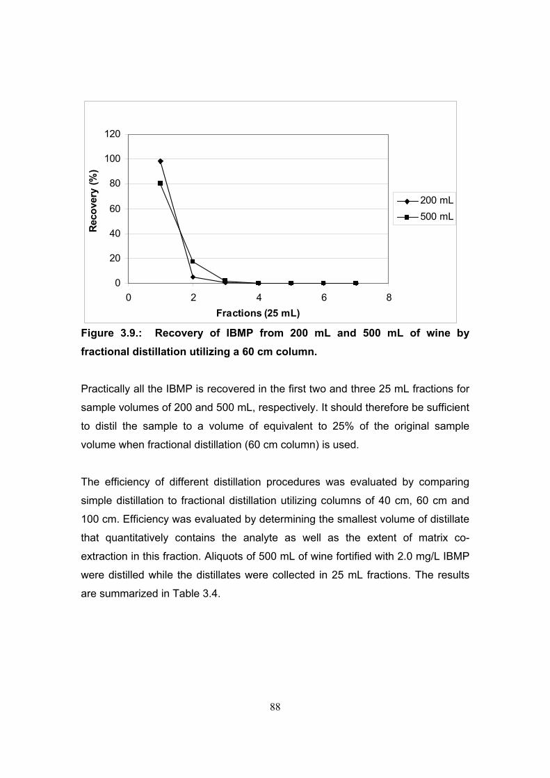
88

0

20

40

60

80

100

120

0 2 4 6 8Fractions (25 mL)

Reco

very

(%)

200 mL500 mL

Figure 3.9.: Recovery of IBMP from 200 mL and 500 mL of wine by fractional distillation utilizing a 60 cm column.

Practically all the IBMP is recovered in the first two and three 25 mL fractions for

sample volumes of 200 and 500 mL, respectively. It should therefore be sufficient

to distil the sample to a volume of equivalent to 25% of the original sample

volume when fractional distillation (60 cm column) is used.

The efficiency of different distillation procedures was evaluated by comparing

simple distillation to fractional distillation utilizing columns of 40 cm, 60 cm and

100 cm. Efficiency was evaluated by determining the smallest volume of distillate

that quantitatively contains the analyte as well as the extent of matrix co-

extraction in this fraction. Aliquots of 500 mL of wine fortified with 2.0 mg/L IBMP

were distilled while the distillates were collected in 25 mL fractions. The results

are summarized in Table 3.4.

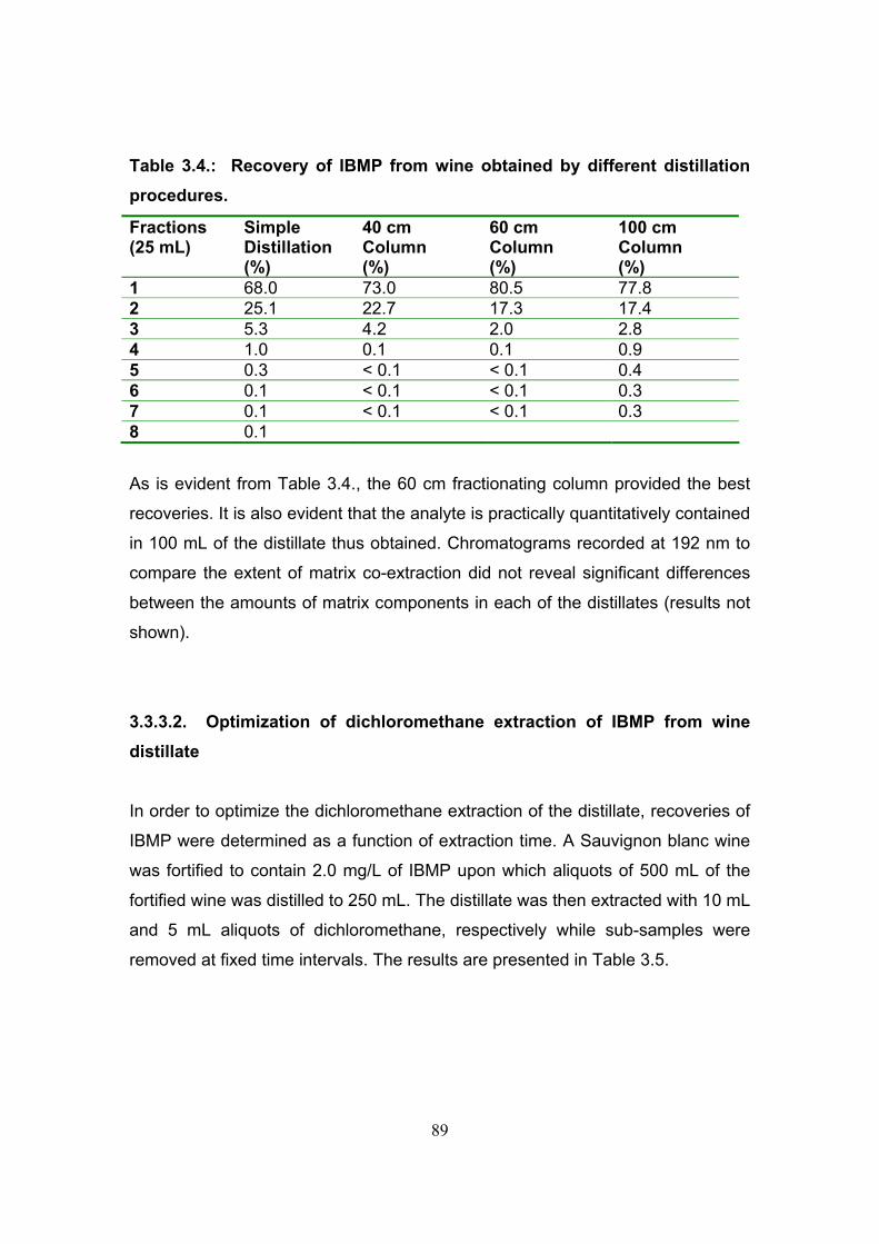
89

Table 3.4.: Recovery of IBMP from wine obtained by different distillation procedures.

Fractions (25 mL)

Simple Distillation (%)

40 cm Column (%)

60 cm Column (%)

100 cm Column (%)

1 68.0 73.0 80.5 77.8 2 25.1 22.7 17.3 17.4 3 5.3 4.2 2.0 2.8 4 1.0 0.1 0.1 0.9 5 0.3 < 0.1 < 0.1 0.4 6 0.1 < 0.1 < 0.1 0.3 7 0.1 < 0.1 < 0.1 0.3 8 0.1

As is evident from Table 3.4., the 60 cm fractionating column provided the best

recoveries. It is also evident that the analyte is practically quantitatively contained

in 100 mL of the distillate thus obtained. Chromatograms recorded at 192 nm to

compare the extent of matrix co-extraction did not reveal significant differences

between the amounts of matrix components in each of the distillates (results not

shown).

3.3.3.2. Optimization of dichloromethane extraction of IBMP from wine distillate

In order to optimize the dichloromethane extraction of the distillate, recoveries of

IBMP were determined as a function of extraction time. A Sauvignon blanc wine

was fortified to contain 2.0 mg/L of IBMP upon which aliquots of 500 mL of the

fortified wine was distilled to 250 mL. The distillate was then extracted with 10 mL

and 5 mL aliquots of dichloromethane, respectively while sub-samples were

removed at fixed time intervals. The results are presented in Table 3.5.

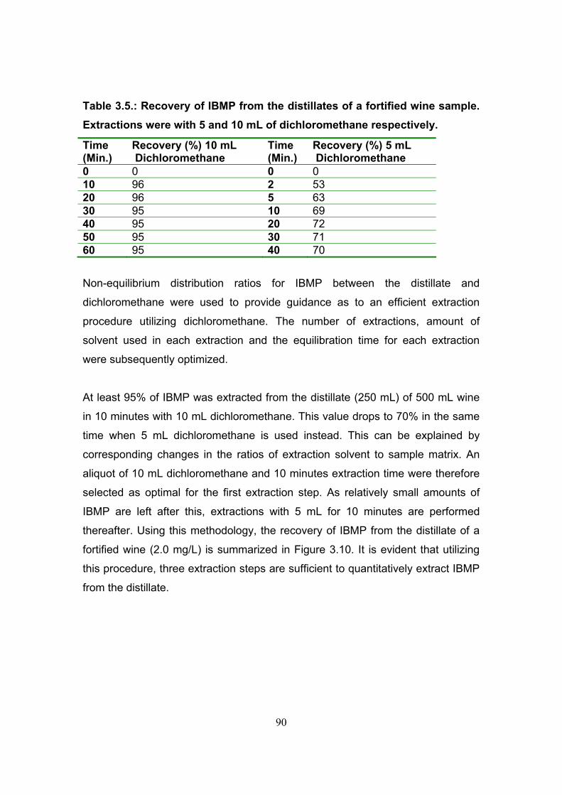
90

Table 3.5.: Recovery of IBMP from the distillates of a fortified wine sample. Extractions were with 5 and 10 mL of dichloromethane respectively.

Time (Min.)

Recovery (%) 10 mL Dichloromethane

Time (Min.)

Recovery (%) 5 mL Dichloromethane

0 0 0 0 10 96 2 53 20 96 5 63 30 95 10 69 40 95 20 72 50 95 30 71 60 95 40 70

Non-equilibrium distribution ratios for IBMP between the distillate and

dichloromethane were used to provide guidance as to an efficient extraction

procedure utilizing dichloromethane. The number of extractions, amount of

solvent used in each extraction and the equilibration time for each extraction

were subsequently optimized.

At least 95% of IBMP was extracted from the distillate (250 mL) of 500 mL wine

in 10 minutes with 10 mL dichloromethane. This value drops to 70% in the same

time when 5 mL dichloromethane is used instead. This can be explained by

corresponding changes in the ratios of extraction solvent to sample matrix. An

aliquot of 10 mL dichloromethane and 10 minutes extraction time were therefore

selected as optimal for the first extraction step. As relatively small amounts of

IBMP are left after this, extractions with 5 mL for 10 minutes are performed

thereafter. Using this methodology, the recovery of IBMP from the distillate of a

fortified wine (2.0 mg/L) is summarized in Figure 3.10. It is evident that utilizing

this procedure, three extraction steps are sufficient to quantitatively extract IBMP

from the distillate.

91

0

20

40

60

80

100

120

0 1 2 3 4 5 6

Extractions

Frac

tion

rem

aini

ng (%

)

Figure 3.10.: Fraction of IBMP remaining in the distillate (250 mL) of 500 mL wine upon extraction with dichloromethane.

The optimized sample preparation procedure utilizing distillation followed by

dichloromethane extraction is summarized below:

• Using an A-grade volumetric flask (500 mL), accurately transfer 500 mL of

wine to a 1 L boiling flask containing a single glass ball. To prevent the

wine from foaming, a spatula tip of tannic acid may be added.

• Distill the wine until a volume of at least 100 mL is collected. The distillate

is collected in a 100 mL volumetric flask.

• Transfer the distillate quantitatively (rinsing with water) to a 500 mL

separating funnel and add 10 mL of dichloromethane as well as a 35 mm

egg-shaped magnet.

• Stopper tightly and stir for 10 minutes at high speed.

• Allow phases to separate and drain the organic phase into a graduated

pear-shaped flask containing 0.5 mL concentrated formic acid.

• Mix the contents of the flask on a vortex mixer and place under gentle

stream of nitrogen.

92

• Repeat with two 5 mL portions of dichloromethane.

• Evaporate the combined dichloromethane fractions from the extract until

less than 0.5 mL of formic acid remains.

• Reconstitute to 1 mL with mobile phase, vortex and transfer to a 1.5 mL

vial.

Figure 3.11.: Comparison between chromatograms obtained for a Sauvignon Blanc wine fortified with 2.0 mg/L IBMP (25 µL injected, top), and the dichloromethane extract of the distillate of the same wine (bottom). Concentration factor 500, 0.1 µL injected. Other HPLC conditions are as specified in section 3.2.2.

The effectiveness of the optimized distillation/extraction procedure was assessed

by the recovery of IBMP from wine using seven extractions of a Sauvignon blanc

wine (fortified with 2.0 mg/L IBMP). Recovery was determined by comparison of

the peak areas obtained for the fortified wine, distillate and reconstituted extracts,

respectively. The recovery for the distillation process was found to be 102%

(RSD = 0.6%), while the total recovery was 110% (RSD = 12%).

min0 2 4 6 8 10 12 14

mAU

0

10

20

30

40

50

60

70

IBMP

min 0 2 4 6 8 10 12 14

mAU

0

10

20

30

40

50

60

70

IBMP

93

In conclusion, it was demonstrated that distillation in combination with

dichloromethane extraction offers a very efficient sample pre-treatment step for

the recovery of IBMP from wine while yielding an effective concentration factor of

500. Figure 3.11. shows chromatograms of a fortified wine and the corresponding

extract.

3.3.4. Evaluation of solid phase extraction for the isolation and pre-concentration of 3-isobutyl-2-methoxypyrazine from wine

As the IBMP molecule posses apolar functionality in addition to the relatively

polar methoxy- and aromatic amine functionalities, normal phase, reversed

phase as well as ion exchange SPE chemistries were evaluated for the SPE

study. Each separation was optimized to determine the capacity of the relevant

SPE cartridge as well as optimal conditions for elution of interferences. Recovery

and the level of enrichment of the analyte from the wine matrix were also

determined in each case.

3.3.4.1 SPE on reversed phase C18 sorbents

In reversed phase chromatography, the stationary phase is apolar and the mobile

phase is a relatively polar solvent.2 The principles that were discussed for

reversed phase liquid chromatography is equally applicable to reversed phase

SPE.

IBMP is expected to be retained strongly via reversed phase mechanism on an

apolar C18 phase as the molecule posses a five-carbon alkyl chain. The column

(200 mg / 3 mL) was conditioned by applying 1 mL of acetonitrile followed by 1

mL of water. Aliquots of 10 mL of wine, fortified to 2.0 mg/L, were applied to the

94

column and the effluent collected in separate fractions for HPLC-UV analysis.

The capacity of the column was determined by analyzing each effluent fraction

and determining the sample volume corresponding to analyte breakthrough.

Breakthrough for IBMP was observed following application of more than 80 mL of

wine. It was therefore assumed that 50 mL is the optimal sample volume (Figure

3.12.).

0

2

4

6

8

10

12

0 20 40 60 80 100 120 140

Total volume loaded (mL)

Pea

k Ar

ea

Figure 3.12.: IBMP breakthrough on C18 SPE column.

Optimal conditions for removal of the sample matrix were then determined by

loading 10 mL of fortified wine onto several columns and applying 1 mL of a

wash solution containing increasing amounts of acetonitrile to each column. The

effluents were collected separately for liquid chromatographic analysis to

determine the fractions that contained eluted analyte. Wash solutions of pure

water and 20, 40, 60 and 80% acetonitrile were evaluated. Breakthrough of IBMP

was observed for wash solutions containing 40% or more of acetonitrile. A

solution of 20% acetonitrile was therefore selected as the most efficient wash

solvent under the described conditions.

95

The efficiency of the optimized C18 SPE process was evaluated by determining

the average recovery of IBMP from wine. An aliquot of 50 mL of fortified wine

(2.0 mg/L) was loaded onto a conditioned column followed by rinsing with 1 mL

of 20% acetonitrile in water. The analyte was then eluted from the column with

three 1 mL portions of acetonitrile and the eluent transferred to a 50 mL pear-

shaped vessel with a 3 mL graduated stem. To prevent volatilization of the

analyte during reduction of the solvent, 0.5 mL concentrated formic acid was

added to the solution. The solution was then evaporated to approximately 0.5 mL

and made up to 1 mL with water, thus producing a concentration factor of 50.

This procedure was repeated three times, and the average recovery of IBMP was

measured as 88% (6.1% RSD, n = 3).

3.3.4.2. SPE on mixed mode reversed phase cartridges

3.3.4.2.1. Direct extraction from wine

New sorbent types for SPE that are designed to have a hydrophilic-lipophilic

balance when used under reversed phase conditions, have recently become

available, and are designed to enhance retention of acidic, basic as well as

neutral compounds. One such phase, marketed under the name Oasis, contains

a sorbent consisting of a copolymer of divinylbenzene and N-vinylpyrrolidone

units. The divinylbenzene units impart lipophilic character to the phase while the

N-vinylpyrrolidone units provide hydrophilic interactions.10

It is expected that IBMP will be strongly retained on the Oasis phase as the

molecule posses an apolar alkyl chain as well as relatively polar aromatic amine-

and methoxy functional groups.

96

The 60 mg / 3 mL Oasis column was conditioned, as prescribed, by applying 1

mL of methanol followed by 1 mL of water. Aliquots of 10 mL of fortified wine

were then applied to the column and the effluent collected separately. The

capacity of the column was determined by analyzing the fractions to determine

the sample volume corresponding to analyte breakthrough. The results indicated

that breakthrough occurred upon loading sample volumes of larger than 100 mL

(Figure 3.13.). It was therefore assumed that 50 mL is the optimal volume of wine

that can be extracted under the described conditions if breakthrough is to be

avoided.

0

0.5

1

1.5

2

2.5

0 20 40 60 80 100 120 140

Total volume loaded (mL)

Pea

k ar

ea

Figure 3.13.: IBMP breakthrough on Oasis column, direct extraction of wine.

Optimal conditions for removal of the sample matrix were determined by loading

10 mL of fortified wine onto several conditioned columns and applying wash

solutions to the column as prescribed by the manufacturer. An initial wash with 1

mL of 5% aqueous methanol was applied to all columns, followed by rinsing with

1 mL of solutions containing 2% ammonia and increasing amounts of methanol in

97

water (10, 20, 30, 40 and 50% methanol were evaluated). A basic rinsing solution

is used to ensure that the analyte remain neutral (and therefore relatively apolar),

thus maximizing retention. Effluents were collected separately for liquid

chromatographic analysis to determine the fractions that contained eluted

analyte. It was found that only a solution of 2% ammonia and 50% methanol in

water, applied after the initial wash, eluted some solute from the column. A

solution of 2% ammonia in 30% methanol was therefore considered to be the

most efficient wash solvent under the described conditions.

The efficiency of the process was evaluated by determining the recovery of IBMP

from wine. An aliquot of 50 mL of fortified wine (2.0 mg/L) was loaded onto a

conditioned column. Elution of matrix components took place in a two-step

process, which consisted of applying first 1 mL of a solution of 5% methanol in

water followed by 1 mL of 2% ammonia and 30% methanol in water. The analyte

was then eluted from the column with three 1 mL aliquots of a solution of 2%

acetic acid in methanol. Protonation of the analyte by the acetic acid renders it

relatively polar to enhance elution from the column. The solvent was then

evaporated and reconstituted as above (for C18 SPE) to produce a concentration

factor of 50. The average recovery for this procedure was 79% (5.1% RSD, n =

3).

3.3.4.2.2. Extraction from the distillate of a wine sample

Distillation of wine samples, prior to solvent extraction, provided an effective

method for elimination of non-volatile matrix components. Subsequent separation

of extracts thus obtained on a C18 column followed by LC-APCI-MS analysis

revealed that some unknown matrix components persisted, which interfered with

the determination of IPMP. As Oasis columns provided the best performance

regarding sample clean-up and pre-concentration, of the SPE products that were

98

evaluated, the use thereof in tandem with distillation was evaluated to eliminate

the said interferon.

The 500 mg / 6 mL Oasis column was conditioned by applying 5 mL of methanol

followed by 5 mL of water. An aliquot of 500 mL wine (fortified to 200 ng/L) was

then distilled utilizing a 60 cm fractionating column and the first 100 mL of the

distillate collected. The distillate was transferred to a 500 mL separating funnel

and extracted with dichloromethane as described in section 3.3.3.2. The

combined extracts were reduced to approximately 2 mL and subsequently

reconstituted in 25 mL 2% ammonia in water for application to the SPE column.

The capacity of the column was determined by analyzing the fraction

corresponding to the last 2 mL of solution that was passed through the column to

ensure complete analyte retention. For these experiments the content of

methoxypyrazines were measured with LC-APCI-MS as outlined in the

experimental section.

Removal of the sample matrix was optimized by applying 1 mL aliquots of rinsing

solvents consisting of 2% ammonia in water and 10 to 90% methanol (in 10%

increments) to the column. Each effluent was collected separately for LC-MS

analysis to determine the fractions that contained eluted analyte.

It was found that a solution of 2% ammonia in 90% methanol eluted measurable

quantities of the analyte from the column. A solution of 2% ammonia and 70%

methanol in water was therefore considered to be the most efficient wash

solvent. It was subsequently confirmed that elution with three 1 mL aliquots of

this (latter) solution did not remove measurable quantities of the 3-alkyl-2-

methoxypyrazines from the column. Elution of the analyte was achieved utilizing

a solution of 5% formic acid in acetone.

Repeatability of the optimized procedure was evaluated by determining the

recovery of IBMP from a wine sample, fortified to contain 200 ng/L IBMP.

99

Aliquots of 500 mL wine were distilled and 100 mL of the distillate collected.

Distillates were extracted with dichloromethane and the combined fractions

reduced under nitrogen, at room temperature, to approximately 2 mL. This

solution was then reconstituted to 25 mL with a solution of 2% ammonia in water

and applied to a pre-conditioned SPE cartridge. The collection vessel was rinsed

three times with 1 mL of water and transferred to the cartridge, prior to washing

with three 1 mL aliquots of 2% ammonia in 70% methanol. Analytes were eluted

from the column with five 2 mL aliquots of a solution of 5% formic acid in

acetone. The solvent was evaporated and the solution reconstituted as before,

thus producing a concentration factor of 500. Residual formic acid served to

protonate the analyte, thus rendering it less volatile. Residues were measured

with LC-APCI-MS. The average recovery of IBMP from the wine matrix was 82%

(RSD = 4.3%, n = 3).

3.3.4.3. Reversed phase SPE on polystyrene-divinylbenzene (PSDVB) cartridges

The polystyrene-divinylbenzene phase is a highly cross-linked polymer that is

unmodified and does not exhibit secondary interactions.11 The phase is suited for

non-selective retention of solutes of low to moderate polarity via a reversed

phase mechanism. The large surface area associated with the polymeric

sorbents imparts a relatively high capacity to the phase.

A PSDVB cartridge was conditioned with 1 mL of acetonitrile followed by 1 mL of

water. Aliquots of 10 mL of wine, fortified with 2.0 mg/L IBMP, were applied

consecutively and each effluent fraction collected separately for HPLC-UV

analysis. After a total volume of 120 mL was loaded without saturation of the

column, the aliquots were increased to 30 mL. A total volume of 570 mL wine

was eventually loaded onto the column without saturation of the phase. It was

therefore assumed that the column has a capacity of at least 500 mL.

100

Elimination of the sample matrix was optimized by loading 10 mL aliquots of

fortified wine onto several columns and applying 1 mL of wash solutions

containing increasing amounts of acetonitrile (20, 40, 60 and 80% in water) to

each column. Each effluent was collected separately for HPLC-UV analysis to

determine the fractions that contained eluted analyte. Since small amounts of

analyte were detected in the 40% acetonitrile fraction, a solution of 20%

acetonitrile was selected as the most efficient wash solvent.

The efficiency was evaluated by determining the average recovery from a wine

fortified with 2.0 mg/L IBMP. An aliquot of 50 mL of wine was loaded onto a

conditioned column. Matrix components were rinsed off with 1 mL of a 20%

solution of acetonitrile in water while the analyte was eluted with three 1 mL

aliquots of acetonitrile. Solvent removal and reconstitution was as before, thus

producing a concentration factor of 50. It should be noted that the phase has the

capacity to extract at least 500 mL of wine and that larger concentration factors

may be realized. The average recovery of IBMP from the wine matrix was 84%

(RSD = 8.3%, n = 3).

3.3.4.4. SPE on normal phase silica sorbents

In normal phase (NP) chromatography, polar compounds are adsorbed from a

relatively apolar environment onto a polar stationary phase.2 On the unmodified

silica phases, the primary interaction is polar, but the silanol groups are ionizable

and can also be utilized as a weak cation exchanger. NP-SPE was evaluated for

removal of apolar interferences by retention of the relatively polar 3-alkyl-2-

methoxypyrazines. The polarity of water generally precludes the use of silica

SPE columns for the extraction of polar compounds from an aqueous

environment.

101

The silica SPE cartridge was conditioned by applying 1 mL of isooctane. Aliquots

of 10 mL of fortified wine were then applied to the column and the effluent

collected separately for liquid chromatographic analysis. The capacity of the

cartridge was determined and analyte breakthrough was observed after 20 mL of

wine was loaded onto the column. This relatively low capacity of the silica phase

may be ascribed to an unfavorable partitioning ratio of the solute between the

polar, aqueous wine matrix and the polar stationary phase. It may therefore be

concluded that the phase is not saturated, but rather that partitioning of the solute

towards the aqueous sample matrix predominates with the result that the solute

elutes without significant retention on the stationary phase.

Matrix removal was evaluated by loading 10 mL of fortified wine onto a single

cartridge and applying 1 mL aliquots of wash solvents of increasing polarity. Only

water-soluble solvents were evaluated to ensure compatibility with the HPLC

method. The effluent was collected separately for HPLC-UV analysis to

determine the fractions that contained eluted analyte. The results were as follows

(Table 3.6.):

Table 3.6.: Determination of optimal conditions for sample clean-up and pre-concentration utilizing normal phase SPE.

Wash Solution Peak area (pA.s) Tetrahydrofuran 11.6 Acetone 5.6 Acetonitrile 3.1 Methanol - Water -

It can be seen that tetrahydrofuran, the least polar, water-soluble solvent

investigated, eluted IBMP from the column. Effective removal of wine matrix

components from the column is therefore not possible under the described

conditions. The efficiency of the silica SPE procedure was considered too low for

effective pre-concentration of IBMP from wine and was not further evaluated.

102

3.3.4.5. SPE on strong and weak cation exchange sorbents

Cation exchange sorbents may be used to extract positively charged (basic)

compounds from aqueous samples via ionic interactions between the charged

solute and the conjugated base of the stationary phase. Residual silanol groups

on the silica support provide secondary polar interactions while the aliphatic or

aromatic links may present secondary apolar interactions. Retained cationic

compounds may be eluted with a solution of high ionic strength, by neutralizing

the charge on the cationic solute, or by eliminating the charge on the stationary

phase. Due to secondary apolar interactions, the addition of an organic modifier

may enhance elution of the solute.

Strong cation exchange sorbents generally consist of sulfonic acid groups

bonded to a silica support via aliphatic or aromatic links. The sulfonic acid group

is characterized by a very low pKa (< 1.0) with the result that it remains ionized

even at low pH. Weak cation exchange sorbents consist of an aliphatic carboxylic

acid bonded to a silica support.9 The carboxylic acid functional group posses a

pKa of approximately 4.8 and is generally used to extract basic compounds

capable of carrying a positive charge at pH 6.8 or higher. Elution of the solute

from the column may be achieved utilizing the same strategies discussed for the

strong cation exchangers.

3.3.4.5.1 Optimization of an SPE procedure on a strong cation exchange sorbent

The Strata SCX cartridge was conditioned by applying 1 mL of methanol followed

by 1 mL of water. It is assumed that the amine functional groups of pyrazines are

protonated and positively charged in the wine matrix which has a typical pH

ranging between 3 and 4.17 Aliquots of 10 mL wine, fortified to 2.0 mg/L, were

applied to various columns followed by a rinsing step with 1 mL water. Analyses

103

of the effluents revealed complete retention of the solute. A variety of strategies

for elution of the solute from the column were then evaluated.

• Elution with concentrated acid (three 1 mL portions of 2 N sulfuric acid).

The proposed mechanisms are a mixture of displacement of the solute by

a concentrated solution of ions and elimination of the charge on the

stationary phase by protonation of the sulfonic acid groups at low pH (the

pH of the 2 N sulfuric acid solution is approximately 0.7).

• Elution with concentrated acid with added organic phase (three 1 mL

portions of 50% 2 N sulfuric acid in methanol). Possible elution

mechanisms involved are ionic strength, neutralization of the charge on

the stationary phase as well addition of an organic modifier to compensate

for secondary apolar interactions.

• Elution with strong base (three 1 mL portions of 2 N sodium hydroxide).

Proposed mechanisms are a mixture of displacement of the solute by a

concentrated solution of ions as well as neutralizing the charge on the

cationic solute. The pH of the 2 N sodium hydroxide solution was

approximately 14.

• Elution with a strong base with added organic phase (three 1 mL portions

of a solution of 50% 2 N sodium hydroxide in methanol). Possible elution

mechanisms are ionic strength, neutralization of the charge on the solute

as well addition of an organic modifier to compensate for secondary apolar

interactions.

It was found that the solute is not eluted from the column with any of the

proposed solvent systems, indicating that the protonated tertiary di-amine

functional group of methoxypyrazines is very strongly retained on this phase. De

Boubee et.al.13 successfully rinsed the solute from a small mass of cation

exchange resin with 10% NaOH, as opposed to ~8% used in this study in

conjunction with 500 mg cartridges. Strong ion exchangers are also known to

irreversible retain very strong ions such as quaternary amines.18

104

3.3.4.5.2. Extraction of methoxypyrazines from the distillate of a wine sample utilizing a strong cation exchange sorbent

Several authors reported the successful use of cation exchange resin for the

isolation of IBMP from the distillates of wine samples.4,5,13,15 As this mechanism

was anticipated to provide excellent clean-up of extracts for subsequent reversed

phase separation, this combination was evaluated. As a relatively large,

concentrated NaOH solution is required for elution of the analyte from the SCX

resin, back-extraction into dichloromethane is essential. Unlike with with gas

chromatography, these extracts then need to be evaporated to remove the

dichloromethane followed by reconstitution in mobile phase so that the solutions

may be compatible with reversed phase liquid chromatographic separation.

An aliquot of 100 mL of the fortified wine sample (200 ng/L) was distilled utilizing

simple distillation and 50 mL of the distillate was collected. An aliquot of 1 mL of

sulfuric acid was added and the solution reconstituted to 100 mL with water. The

500 mg SCX column was conditioned by applying 1 mL of methanol followed by

1 mL of water. The total volume of the acidified distillate (100 mL) was then

applied to the column. The capacity of the column was determined by analyzing

the fraction corresponding to the last 2 mL of distillate that was passed through

the column. It was found that no analyte breakthrough occurred during the

sample loading step.

The column was rinsed with 1 ml of a solution of 10% methanol in water.

Analysis of the rinse revealed that no measurable quantities of the analyte were

removed during this step.

Optimal conditions for elution of the analyte from the column were determined by

applying 1 mL aliquots of a solution of 5% sodium hydroxide in 50% methanol to

105

the column. Residues were extracted (from elution solution) into

dichloromethane. Aliquots of 0.5 mL concentrated formic acid were then added to

the dichloromethane fractions followed by evaporation to less than 0.5 mL.

Extracts were then reconstituted in 2.5 mL of water for analysis. From the results

it was evident that elution of the solute may be affected with at least six 1 mL

aliquots of 5% sodium hydroxide in 50% methanol.

The optimal conditions for the extraction of the analyte from the elution solution

(5% sodium hydroxide in 50% methanol) were then determined by performing

repeated extractions with 2.5 mL dichloromethane. It was found that three

extractions with 2.5 mL dichloromethane ensure complete recovery of the solute

from the elution solution.

The efficiency of the optimized distillation/SPE (SCX) procedure was evaluated

by determining the average recovery of IBMP from the distillate of fortified wine

samples (200 ng/L). Aliquots of 100 mL of wine were distilled and 50 mL of the

distillate collected. Aliquots of 1 mL sulfuric acid were then added to each

distillate prior to reconstitution to 100 mL with water. These solutions were

applied to pre-conditioned SCX cartridges. The collection vessels were rinsed

with water and the water passed through the respective columns. After rinsing

the cartridges with 1 mL 10% methanol in water, the analyte were eluted with five

2 mL aliquots of 5% sodium hydroxide in 50% methanol. The eluents were

subsequently extracted with three 2.5 mL aliquots of dichloromethane. To the

dichloromethane fraction were then added 0.5 mL concentrated formic acid upon

which the fraction was evaporation to 0.5 mL. Finally the extracts were

reconstituted in 1 mL of water for analysis, yielding a concentration factor of 100.

Even though the average recovery (n = 3) was 95%, the repeatability of this

procedure was very poor, as reflected by an RSD value of 43%. It is anticipated

that the poor repeatability of this procedure results from the extraordinary large

number of steps that are required to obtain the extract in a solution that is

compatible with reversed phase liquid chromatographic separation. When

106

dissolved in the strong sodium hydroxide solution, the IBMP molecule is also

expected to be uncharged and relatively volatile. Moreover, it is expected that the

high ionic strength of the sodium hydroxide solution may enhance partitioning of

the neutral analyte into the vapor phase, similarly to ionic strength adjustment for

SPME sampling. Losses by volatilization of the analyte may thus occur during

this step.

3.3.4.5.3. SPE on weak cation exchange sorbents

A weak cation exchange cartridge was conditioned by applying 1 mL of methanol

followed by 1 mL of water. As before, it can be assumed that methoxypyrazines

are protonated in the wine matrix.17 An aliquot of 10 mL of fortified wine

containing 2.0 mg/L of IBMP, was applied to the cartridge, followed by rinsing

with 1 mL water. Analyses of the effluents revealed that the solute passed

through the column un-retained under these conditions. Since the pH of wine is

below the pKa of the carboxylic acid functional group of the stationary phase, it is

presumed that protonation of the stationary phase is responsible for this

observation. This precludes the use of this phase for the extraction of the solute

from wine without pH adjustment.

The experiment was therefore repeated with a fortified wine of which the pH was

adjusted to approximately 9 by the addition of 5% (m/v) sodium hydroxide.

Analysis of the effluent revealed that practically no retention is achieved under

these conditions. One possible explanation for this result is that the charge on

the aromatic amine groups is eliminated under these conditions, with the result

that the (uncharged) analyte passes through the cation exchange column un-

retained. In conclusion, it was found that the weak cation exchange sorbent was

unsuitable for the extraction of IBMP from wine samples.

107

3.3.5. Evaluation of stir bar sportive extraction (SBSE) for the isolation and pre-concentration of IBMP from wine

SBSE is often used for headspace sampling of volatile analytes in conjunction

with thermal desorption and subsequent gas chromatographic analysis.17 The

technique is however equally amenable to liquid sampling as well as liquid

desorption, with the result that it can be used with liquid chromatography as

well.8

The efficiency of SBSE utilizing a polydimethylsiloxane (PDMS) phase was

evaluated for sorption of IBMP from wine samples. The technique was evaluated

for direct extraction by stirring in wine samples as well as sorption of volatile

material from the headspace of an agitated wine sample. PDMS is an apolar

phase and is expected to display affinity towards IBMP.

Since extraction in SBSE is based on the partitioning into the PDMS phase, and

therefore an equilibrium process, extraction time of 1 hour was allowed for both

absorption- and desorption steps. The stir bar was re-activated between

experiments by thermal desorption at 220°C for three hours under constant

nitrogen flow of 175 mL/min. Recovery of IBMP from the wine samples was

determined by analyzing the wine before and after extraction as well as the

extract after liquid desorption of the stir bar.

3.3.5.1. SBSE in headspace mode

An aliquot of 5 mL of fortified wine (2.0 mg/L IBMP) and 1.5 g of sodium chloride

were transferred to a 25 mL vial containing a small Teflon-coated stir-bar. The

PDMS-coated stir-bar was placed in the headspace of the sample utilizing a

glass adapter, upon which the vial was sealed. The sample solution was stirred

for 1 hour during the extraction step. The stir-bar was subsequently removed and

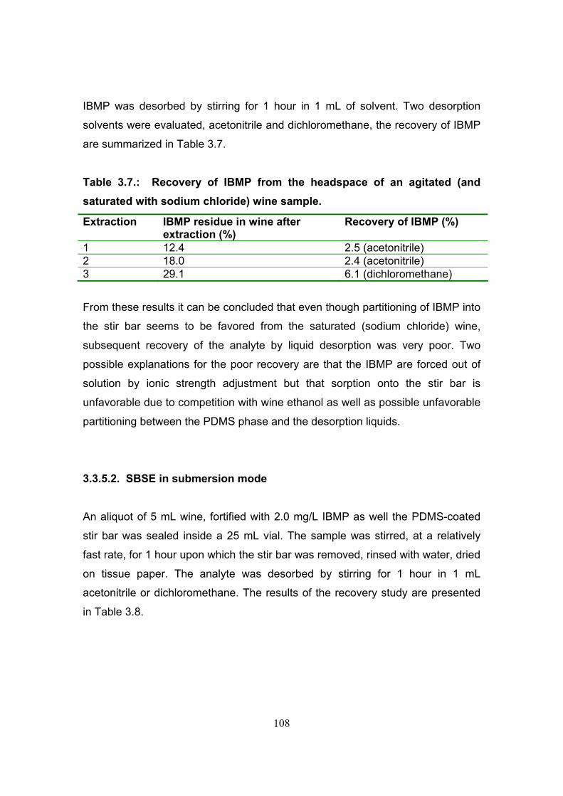
108

IBMP was desorbed by stirring for 1 hour in 1 mL of solvent. Two desorption

solvents were evaluated, acetonitrile and dichloromethane, the recovery of IBMP

are summarized in Table 3.7.

Table 3.7.: Recovery of IBMP from the headspace of an agitated (and saturated with sodium chloride) wine sample.

Extraction IBMP residue in wine after extraction (%)

Recovery of IBMP (%)

1 12.4 2.5 (acetonitrile) 2 18.0 2.4 (acetonitrile) 3 29.1 6.1 (dichloromethane)

From these results it can be concluded that even though partitioning of IBMP into

the stir bar seems to be favored from the saturated (sodium chloride) wine,

subsequent recovery of the analyte by liquid desorption was very poor. Two

possible explanations for the poor recovery are that the IBMP are forced out of

solution by ionic strength adjustment but that sorption onto the stir bar is

unfavorable due to competition with wine ethanol as well as possible unfavorable

partitioning between the PDMS phase and the desorption liquids.

3.3.5.2. SBSE in submersion mode

An aliquot of 5 mL wine, fortified with 2.0 mg/L IBMP as well the PDMS-coated

stir bar was sealed inside a 25 mL vial. The sample was stirred, at a relatively

fast rate, for 1 hour upon which the stir bar was removed, rinsed with water, dried

on tissue paper. The analyte was desorbed by stirring for 1 hour in 1 mL

acetonitrile or dichloromethane. The results of the recovery study are presented

in Table 3.8.

109

Table 3.8.: Recovery of IBMP from a wine sample (direct stirring).

Extraction IBMP residue in wine after extraction (%)

Recovery of IBMP (%)

1 84.1 10.0 (acetonitrile) 2 No result. 25.0 (acetonitrile) 3 86.1 7.6 (dichloromethane)

These results indicate that partitioning of the relatively polar IBMP into the PDMS

phase is not favored. Subsequent liquid extraction provided relatively good

removal of the extracted analyte, in contrast to the result obtained for headspace

sampling. It can be concluded that SBSE (in both headspace and immersion

modes) in combination with liquid desorption is not an effective sample

pretreatment step for the analysis of methoxypyrazines in wine samples by

HPLC.

A possible explanation for the poor performance of SBSE may be that the

ethanol content of the wine interfered with efficient sorption of IBMP into the

phase. Successful application of the SPME technique, utilizing PDMS-DVB

fibers, was reported where the wine was acidified and distilled to remove the

ethanol followed by neutralization and ionic strength adjustment, prior to

extraction.6

3.4. Conclusions

Various sample clean-up and pre-concentration strategies were evaluated

including distillation, solvent extraction and solid phase extraction.

It was demonstrated that dichloromethane solvent extraction is capable of

quantitative extractive pre-concentration of mg/L levels of IBMP from Sauvignon

blanc wine. The average recovery was better 90% with RSD of 11%, while a

concentration factor of 200 was attained utilizing direct solvent extraction with

110

dichloromethane. A total of 25 mL of dichloromethane is used in the process with

total equilibration time of 60 minutes. Total time per sample is 2 hours.

Distillation may be used in tandem with the described solvent extraction

procedure to improve the efficiency of the sample preparation procedure.

Distillation imparts an extra measure of selectivity to the process thus reducing

the matrix of the extract. The distillates also require less solvent for extraction

with reduced equilibration time. As the evaporation of solvent from the extract is

very time consuming, reduction of the amount of solvent required will make the

process more time-efficient. The efficiency of the sample preparation procedure

is also improved as larger effective volumes of sample may be extracted

resulting in increased concentration factors. When used in tandem, the average

recovery of the combined processes was 110% with RSD of 12% while yielding a

concentration factor of 500. A total of 20 mL of dichloromethane is used in the

process with total equilibration time of 30 minutes. Total time per sample is 90

minutes.

When solvent extraction is performed on the distillate, the mixture can be stirred

at a fast rate thereby speeding up the process. The dichloromethane extracts

must not be evaporated to complete dryness as losses of IBMP then occur while

the addition 0.5 mL concentrated formic acid prior to evaporation ensures

protonation of the analyte thereby rendering it less volatile (ionic state less

volatile than neutral molecule).

The efficiency of various SPE phases was evaluated for direct extraction of IBMP

from the wine matrix. Table 3.9. summarizes the results obtained with various

phases.

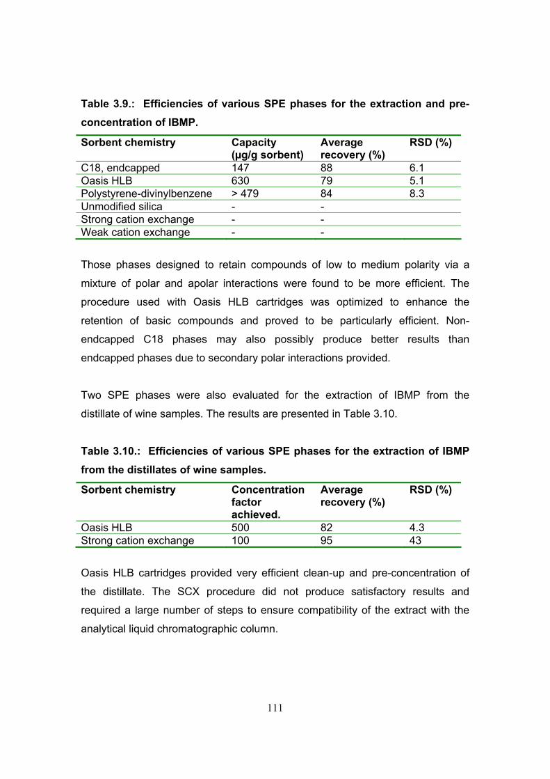
111

Table 3.9.: Efficiencies of various SPE phases for the extraction and pre-concentration of IBMP.

Sorbent chemistry Capacity (µg/g sorbent)

Average recovery (%)

RSD (%)

C18, endcapped 147 88 6.1 Oasis HLB 630 79 5.1 Polystyrene-divinylbenzene > 479 84 8.3 Unmodified silica - - Strong cation exchange - - Weak cation exchange - -

Those phases designed to retain compounds of low to medium polarity via a

mixture of polar and apolar interactions were found to be more efficient. The

procedure used with Oasis HLB cartridges was optimized to enhance the

retention of basic compounds and proved to be particularly efficient. Non-

endcapped C18 phases may also possibly produce better results than

endcapped phases due to secondary polar interactions provided.

Two SPE phases were also evaluated for the extraction of IBMP from the

distillate of wine samples. The results are presented in Table 3.10.

Table 3.10.: Efficiencies of various SPE phases for the extraction of IBMP from the distillates of wine samples.

Sorbent chemistry Concentration factor achieved.

Average recovery (%)

RSD (%)

Oasis HLB 500 82 4.3 Strong cation exchange 100 95 43

Oasis HLB cartridges provided very efficient clean-up and pre-concentration of

the distillate. The SCX procedure did not produce satisfactory results and

required a large number of steps to ensure compatibility of the extract with the

analytical liquid chromatographic column.

112

The PSDVB phase provided the capacity to extract the required volume of wine

(500 mL) to affect a concentration factor of 500, but the practicality of loading this

volume on standard SPE cartridges generally rendered this technique unsuitable

for use in this study. Oasis HLB produced the same concentration factor when

utilized to extract the reconstituted (2% aqueous ammonia) dichloromethane

extract of a (distilled) wine sample and provided very efficient sample clean-up.

The procedure was however very elaborate and did not remove critical

interferons as was evident upon C18 separation of the extracts and APCI-LC-MS

analysis.

The efficiency of the polydimethylsiloxane coated stir-bar for the absorption of

IBMP from wine samples was very low. Sala et.al.6 reported the successful use

of polydimethylsiloxane-divinylbenzene coated fibers in the headspace solid-

phase microextraction of IBMP from wine with excellent recovery. The procedure

described however involves distillation of an acidified (pH 0.5) wine sample to

remove ethanol and other volatile interfering matrix components with subsequent

neutralization, in conjunction with high ionic strength, for headspace extraction of

various 3-alkyl-2-methoxypyrazines. It may therefore be assumed that that

ethanol and other wine matrix components, that were not removed prior to

extraction in this study, prohibited efficient recovery of IBMP from unmodified

wine samples by saturation of the phase.

It can be concluded that fractional distillation (60 cm column) followed by

dichloromethane solvent extraction produced very efficient pre-concentration (a

factor of 500) of wine samples. The recovery obtained was 110% with RSD of

12%. Additional sample clean-up was achieved by further extracting the sample

solution with Oasis HLB SPE columns, but this degraded the precision (82%

recovery, RSD = 4.3%) and time-efficiency of the procedure. The procedure

utilizing distillation in combination with dichloromethane solvent extraction as

described in section 3.3.3.2. was considered as most suited for use in the

investigation.

113

REFERENCES



WINES, Wynboer, (2004).

(2) D. A. Skoog, D.M. West, F.J. Holler, FUNDAMENTALS OF ANALYTICAL

CHEMISTRY, 7th ed.(1996), Saunders College Publishing, Orlando, 764 -

774.

(3) SAMPLE PREPARATION; SOLID PHASE EXTRACTION AND

MEMBRANE FILTRATION, Machery-Nagel GmbH & Co. KG P.O. Box

101352, D-52313 Duren, Germany, 2 - 9.


METHOXYPYRAZINES IN RED WINES BY STABLE ISOTOPE

DILUTION GAS CHROMATOGRAPHY-MASS SPECTROMETRY, J. Agr.

Food Chem., 42 (1994), 1734 - 1738.


AFFECT BERRY METHOXYPYRAZINE CONCENTRATION, Am. J. Enol.

Vitic., 50 (1999), 194 - 198.

(6) C. Sala, M. Mestres, M.P. Marti, O. Bustro, J. Guasch, HEADSPACE

SOLID-PHASE MICROEXTRACTION OF ANALYSIS OF 3-ALKYL-2-

METHOXYPYRAZINES IN WINE, J. Chromatogr. A, 953 (2002), 1 – 6

(7) E. Baltussen, P. Sandra, F. David, C. Cramers, STIR BAR SORPTIVE

EXTRACTION (SBSE), A NOVEL EXTRACTION TECHNIQUE FOR

AQUEOUS SAMPLES: THEORY AND PRINCIPLES, J. Microcolumn

Sep., 11 (1999), 737 – 747.

(8) A. De Villiers, G. Vanhoenacker, F. Lynen, P. Sandra, STIR BAR

SORPTIVE EXTRACTION-LIQUID DESORPTION APPLIED TO THE

ANALYSIS OF HOP-DERIVED BITTER ACIDS IN BEER BY MICELLAR

ELECTROKINETIC CHROMATOGRAPHY, Electrophoresis 25 (2004),

WILEY-VCH Verlag GmbH & Co. KGaA, Weinheim, 1 - 7.

114

(9) CATALOGUE OF SAMPLE PREPARATION PRODUCTS AND

SERVICES, International Sorbent Technology Ltd., Dyffryn Business Park,

Hengoed, Mid Glamorgan, UK CF82 7RJ.

(10) Waters Corporation, 34 Maple Street Milford, MA, 01757 U.S.A.

(11) CHROMATOGRAPHY COLUMNS AND SUPPLIES 04/05 CATALOG,

Phenomenex, 411 Madrid Avenue Torrance, CA 90501-1430, U.S.A.

(12) Y. Kotseridis, A. Anocibar Beloqui, A. Bertrand, J. P. Doazan, AN

ANALYTICAL METHOD FOR STUDYING THE VOLATILE

COMPONENTS OF MERLOT NOIR CLONE WINES, Am. J. Enol. Vitic.

49 (1998), 44 - 48.

(13) D. Roujou De Boubee, C. Van Leeuwen, D. Dubourdieu,

ORGANOLEPTIC IMPACT OF 2-METHOXY-3-ISOBUTYLPYRAZINE ON

RED BORDEAUX AND LOIRE WINES, EFFECT OF ENVIRONMENTAL

CONDITIONS ON CONCENTRATIONS IN GRAPES DURING

RIPENING, J. Agric. Food Chem., 48 (2000) 4830 – 4834.

(14) D. R. Lide, CRC HANDBOOK OF CHEMISTRY AND PHYSICS, 86th ed.

(2005 – 2006), CRC Press, 6000 Broken Sound Parkway NW, Suite 300

Boca Raton FL.


METHOXYPYRAZINES IN SAUVIGNON BLANC GRAPES AND WINE,

Am. J. Enol. Vitic., 42 (1991), 103 – 108.

(16) P. J. Hartmann, H. M. McNair, B. W. Zoecklein, MEASUREMENT OF 3-

ALKYL-2-METHOXYPYRAZINE BY HEADSPACE SOLID-PHASE

MICROEXTRACTION IN SPIKED MODEL WINES, Am. J. Enol. Vitic., 53

(2002), 285 - 288.

(17) R. S. Jackson, WINE SCIENCE: PRINCIPLES, PRACTICE AND

PERCEPTION, 2 nd ed.(2000), Academic Press, San Diego, 240.

(18) M. C. McMaster, LC/MS A PRACTICAL USER’S GUIDE, (2005) John

Wiley & Sons Inc., 111 River Street, Hoboken, NJ 07030.

115

CHAPTER 4

Development of an optimized liquid chromatography - mass spectrometric method for trace level quantitation

of selected 3-alkyl-2-methoxypyrazines

4.1. Introduction and objectives

The objective of this Chapter is to describe the development of an optimized

liquid chromatography mass spectrometric (LC-MS) method for sensitive and

selective measurement of selected 3-alkyl-2-methoxypyrazines in wine namely 3-

isobutyl-2-methoxypyrazine (IBMP), 3-isopropyl-2-methoxypyrazine (IPMP), 3-

sec-butyl-2-methoxypyrazine (SBMP), 3-ethyl-2-methoxypyrazine (EMP) and 3-

methyl-2-methoxypyrazine (MMP). As the expected levels of the analytes in wine

are very low, a sample preparation step affecting pre-concentration of a factor of

500 (described in Chapter 3) was used. Extracts were separated utilizing

reversed phase liquid chromatography followed by atmospheric pressure

ionization for mass spectrometric analysis. To facilitate accurate trace level

quantitation of the components of interest in the presence of concentrated matrix

elements, experiments were aimed at determining the optimal experimental

parameters pertaining to the separation, ionization, fragmentation and detection

of the substances under investigation.

116

4.2. Experimental 4.2.1. Materials

Only high purity solvents and chemicals were used throughout the experiment.

Acetonitrile, dichloromethane and tannic acid were from Merck (Darmstadt,

Germany), IBMP, IPMP, SBMP, EMP, MMP, methanol and ethanol from Aldrich

(Sigma-Aldrich, South Africa) hexane from Burdick & Jackson (Honeywell

International, U.S.A.) and formic acid from Associated Chemical Enterprises

(ACE, South Africa).


on an analytical balance followed by dilution utilizing A-grade volumetric


standards were prepared in 10% ethanol. For the exploratory work, where the

efficiency of octadecyl and polystyrene-divinylbenzene columns were compared

utilizing LC-UV, working standards were prepared in 50% acetonitrile to

correspond approximately to the gradient starting concentration. Wine samples

for the recovery studies were fortified by adding appropriate amounts of

standards followed by distillation, solvent extraction and pre-concentration as

described in Chapter 3.

4.2.2. Instrumentation

The LC-MS system utilized was a Waters Alliance 2695 liquid chromatograph

(Waters Corporation, Milford, U.S.A.), equipped with a six-port switching valve

and Waters Micromass Quattro Premier XE tandem quadrupole mass

spectrometric detector (Manchester, U.K.). Nitrogen gas for the atmospheric-

pressure interface was supplied by a generator while bottled argon (5.0) was

used as collision gas. Post-column addition of reagents was done with a

117

Shimadzu LC-6A liquid chromatography pump and Shimadzu SCL-6B system

controller (Shimadzu Corporation, Kyoto, Japan), synchronized with the LC-MS

system. Analytes were ionized utilizing either of two atmospheric pressure

ionization techniques namely electrospray ionization (ESI) and atmospheric

pressure chemical ionization (APCI). The mass spectrometer was operated in

multiple reaction monitoring (MRM) mode. Mass spectral information was

acquired by direct infusion of standards of 3 to 8 mg/L of the components of

interest via an integrated syringe pump.

For the preliminary evaluation of the efficiency of octadecyl and polystyrene-

divinylbenzene columns, an Agilent 1100 LC system (Agilent Technologies,

Waldbronn, Germany) fitted with quaternary pump, autosampler, column oven

and UV-visible diode array detector was used. The mobile phase consisted of

various acetonitrile/water gradients. The columns were a Luna C18 (150 x 4.6

mm) with 3 µm particles and a PolymerX polystyrene-divinylbenzene column

(150 x 4.1 mm) with 3 µm particles (both Phenomenex, Torrance, U.S.A.). The

column-temperature was 30°C and variable injection volumes were used. The

chromatographic signal at 292 nm was acquired while spectra between 190 and

400 nm were recorded. All columns evaluated during the course of the study are

summarized in Table 4.1.

A Waters API Q-TOF Ultima LC-MS system was used to perform accurate mass

determinations of the molecular- and fragment ions of the methoxypyrazines.

Ionization was performed using positive ESI with a capillary voltage of 3.5 kV.

The cone voltage was 35 V while the source and desolvation temperatures were

100 and 250 °C respectively. Desolvation gas flow was 200 L/h and cone gas

flow 50 L/h. The collision energy for MS/MS mode of operation was 20 eV.

118

Table 4.1.: Description of columns used in the investigation.

Phase Manufacturer / brand name

Dimensions

C18 Phenomenex Luna

150 x 4,6 mm, 3 µm

Polystyrene-divinylbenzene

Phenomenex PolymerX

150 x 4,1 mm, 3 µm

Phenyl hexyl Phenomenex Luna

250 x 4,6 mm, 5 µm

C8 Agilent Xorbax Eclipse XDB C8

150 x 4.6 mm, 5 µm

C5 Phenomenex Luna

150 x 4,6 mm, 5 µm

CN Phenomenex Luna

250 x 4,6 mm, 5 µm 50 x 4.6 mm, 5 µm


4.3.1. Initial selection of chromatographic separation mode

The 3-alkyl-2-methoxypyrazines under investigation are relatively apolar

molecules and are expected to be retained strongly on reversed phase columns.

Strong solute retention may facilitate elution with a mobile phase that contains a

relatively high proportion of organic modifier as well as potential separation of the

solute from matrix interferences via a gradient. Efficient removal of the elution

solvent during the ionization process is critical for optimal introduction of the ions

into the mass spectrometer and hence method sensitivity. Solvent evaporation

and ionization are also more efficient from a mobile phase that contains a higher

proportion of an appropriate volatile organic modifier. Moreover, co-eluting matrix

elements may interfere with the efficient ionization and mass spectrometric

determination of target compounds and separation of interferences may therefore

be critical for method performance. For this reason the initial part of this

investigation focused on the choice of optimal chromatographic conditions, taking

into account these considerations.

119

4.3.1.1. Evaluation of C18 and polystyrene-divinylbenzene phases for the reversed phase separation of various 3-alkyl-2-methoxypyrazines

The efficiency of octadecyl and polystyrene-divinylbenzene phases was

evaluated for the reversed phase separation of five 3-alkyl-2-methoxypyrazines.

The objective was to identify the phase that offers the best resolution as well as

strongest retention of the analytes, with consequent higher proportion of organic

modifier in the mobile phase at the time of elution.

A standard was analyzed by the liquid chromatographic method with UV

detection described in the experimental section. The gradient used for elution of

the analytes from the C18 column was as follows: Initially 50% acetonitrile for 30

seconds, 50 to 95% acetonitrile in 7 minutes, 95% acetonitrile for 4 minutes. The

flow-rate in the separation was deliberately restricted to 0.5 mL/minute as it was

envisaged that this separation would eventually be used in conjunction with

electrospray ionization and therefore necessitate lower flow rates.

As expected, the degree of retention on the apolar phases increased with the

number of carbon atoms and their arrangement, in the bonded alkyl chain. The

order of elution was MMP, EMP, IPMP, IBMP and SBMP (Figure 4.1.).

120

Figure 4.1.: Standard of MMP (27 ng), EMP (26 ng), IPMP (25 ng), IBMP (96 ng), SBMP (24 ng), in 50% acetonitrile, C18 phase, 150 x 4.6 mm x 3 µm. Signal recorded at 292 nm.

The gradient used for elution of the analytes from the polystyrene-divinylbenzene

phase started at 45% acetonitrile for 1 minute, increased to 75% acetonitrile in 7

minutes, followed by 75% acetonitrile for 2 minutes. The flow-rate was restricted

to 0.5 mL/minute for the reasons discussed earlier (Figure 4.2.).

min0 2 4 6 8 10 12 14

mAU

- 5

0

5

10

15

20

MMP EMP IPMP

IBMP

SBMP

min0 2 4 6 8 10 12 14

mAU

0

5

10

15

20

MMP EMPIPMP

IBMP

SBMP

121

Figure 4.2.: Standard of MMP (27 ng), EMP (26 ng), IPMP (25 ng), IBMP (96 ng), SBMP (24 ng), in 50% acetonitrile, polystyrene-divinylbenzene phase, 150 x 4.6 mm x 3 µm. Signal recorded at 292 nm.

The peaks are clearly better resolved on the C18 phase and the corresponding

fraction of organic solvent in the mobile phase is also greater than is the case on

the polystyrene-divinylbenzene phase. Any attempt to increase the fraction of

organic solvent in the mobile phase in the separation on the latter phase resulted

in a severe loss of resolution. The C18 phase was therefore provisionally

selected for performing the separations in the investigation. It should be noted

that the separations were performed at less than optimal mobile phase flow-rates

in both instances as the purpose here was to compare the efficiency of the two

phases. As it was envisaged that the separation method would eventually be

used in conjunction with electrospray ionization, the evaluation was carried out at

relatively low (less than optimal) flow-rates.

min 0 2 4 6 8 10 12

mAU

- 5

0

5

10

15

20

MMP EMP IPMP

IBMP

SBMP

min 0 2 4 6 8 10 12

mAU

-

0

5

10

15

20

MMP EMP IPMP

IBMP

SBMP

122

4.3.2. Determination of the optimal flow rate in the chromatographic separation utilizing 4.6 mm diameter columns

It is imperative to optimize flow-rates in chromatographic separations in order

maximize the plate count and to achieve optimal signal-to-noise ratios for peaks

of interest. The optimal flow rate on the C18 column (150 x 4.6 mm) was

determined by performing a series of injections of a standard of IBMP at different

flow rates. The mobile phase in the isocratic separation consisted of 88%

aqueous acetonitrile with 1% formic acid. Mass spectrometric detection with

electrospray ionization was utilized in these experiments. The number of

theoretical plates (N) for each separation was determined as follows:1

N = 5.54 (tR / W1/2)2 (8)

Where tR is retention time and W1/2 the peak width at half-height.1 It is evident

from the results summarized in Figure 4.3. that the optimal flow rate on the 4.6

mm diameter column is approximately 1 mL/minute, correlating with the value

expected for small organic molecules.

123

15

17

19

21

23

25

27

29

31

0.3 0.5 0.7 0.9 1.1 1.3

Flowrate (mL/minute)

N (x

100

0)

Figure 4.3.: Column efficiency at various flow rates.

4.3.3. Determination of optimal ionization parameters for the LC-MS analysis of methoxypyrazines

Target compounds, upon elution from the column, need to be ionized in order to

draw them into the mass spectrometer for analysis. The interface between the

liquid chromatograph and the mass spectrometric detector must be capable of

removing most of the elution solvent while efficiently conferring a charge to the

target species. The charged species should then selectively be drawn into the

mass spectrometer. As the objective of the study is to measure trace level

components in a complex matrix, it is imperative to optimize the selective

ionization and introduction of these components in order to confer the highest

possible level of sensitivity to the method. Table 4.2. presents some relevant

chemical data of the substances under investigation:

124

Table 4.2.: Chemical data of the 3-alkyl-2-methoxypyrazines.2

Substance Molecular formula Molecular weight (Da) MMP C6H8N2O 124.14 EMP C7H10N2O 138.17 IPMP C8H12N2O 152.20 IBMP C9H14N2O 166.22 SBMP C9H14N2O 166.22

Methoxypyrazines are aromatic bases with pairs of nonbonding electrons

available to abstract a proton and form positively charged species. As the

protonated, cationic species are still aromatic, it is expected that it will react

readily to produce stable cations. The protonation may proceed as follows

(Figure 4.4.) with the positive charge residing on the no.1 nitrogen, activated by

the methoxy group.3

N

N O

CH3

R N

N+

O

CH3

R

H

H+

H+

H+-

Where R = CH3 or CH2CH3 or CH(CH3)2 or CH2CH(CH3)2 or CH(CH3)CH2CH3

Figure 4.4.: Protonation of the 3-alkyl-2-methoxypyrazines.

Two atmospheric pressure ionization techniques capable of positive mode

ionization were available with the instrument used in this study, namely

electrospray ionization (ESI) and atmospheric pressure chemical ionization

(APCI). As the methoxypyrazines will be measured in multiple reaction

monitoring (MRM) mode, it is imperative that the introduction of precursor

molecular ions is optimized in order to measure resulting daughter ions at optimal

sensitivity.

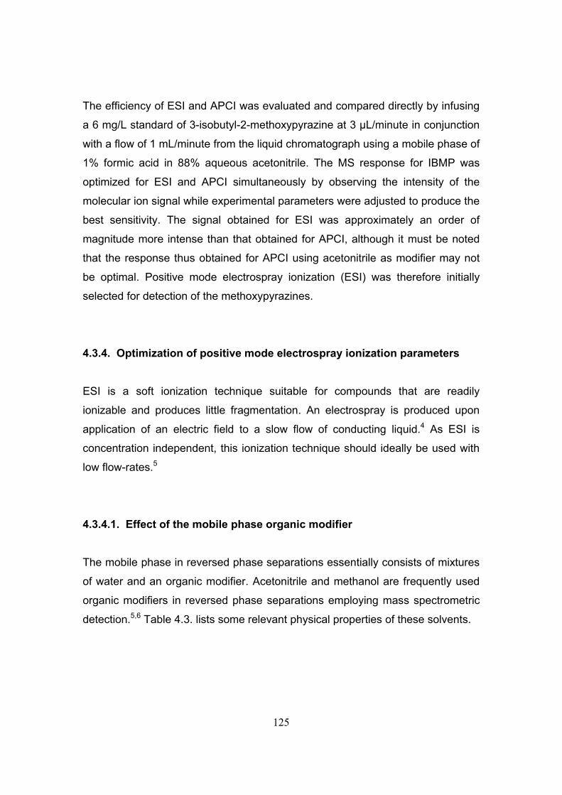
125

The efficiency of ESI and APCI was evaluated and compared directly by infusing

a 6 mg/L standard of 3-isobutyl-2-methoxypyrazine at 3 µL/minute in conjunction

with a flow of 1 mL/minute from the liquid chromatograph using a mobile phase of

1% formic acid in 88% aqueous acetonitrile. The MS response for IBMP was

optimized for ESI and APCI simultaneously by observing the intensity of the

molecular ion signal while experimental parameters were adjusted to produce the

best sensitivity. The signal obtained for ESI was approximately an order of

magnitude more intense than that obtained for APCI, although it must be noted

that the response thus obtained for APCI using acetonitrile as modifier may not

be optimal. Positive mode electrospray ionization (ESI) was therefore initially

selected for detection of the methoxypyrazines.

4.3.4. Optimization of positive mode electrospray ionization parameters

ESI is a soft ionization technique suitable for compounds that are readily

ionizable and produces little fragmentation. An electrospray is produced upon

application of an electric field to a slow flow of conducting liquid.4 As ESI is

concentration independent, this ionization technique should ideally be used with

low flow-rates.5

4.3.4.1. Effect of the mobile phase organic modifier

The mobile phase in reversed phase separations essentially consists of mixtures

of water and an organic modifier. Acetonitrile and methanol are frequently used

organic modifiers in reversed phase separations employing mass spectrometric

detection.5,6 Table 4.3. lists some relevant physical properties of these solvents.

126

Table 4.3.: Physical properties of the organic modifiers studied during the optimization of positive mode electrospray ionization parameters7,8

Solvent Molecular weight (Da)

Boiling point (°C)

Polarity index

Viscosity (m Pa s)

Acetonitrile 41.05 81.7 5.8 0.369 Methanol 32.04 64.6 5.1 0.544 Water 18.02 100.0 9.0 0.890

Electrospray ionization efficiency was evaluated in elution systems of aqueous

acetonitrile and methanol. Sample introduction was by direct infusion of a

standard (3 mg/L) at 5 µL/minute via a syringe pump in conjunction with a flow of

0.3 mL/minute from the liquid chromatograph at the various mobile phase

compositions. The MS response (scan mode) was optimized by observing the

intensity of the molecular ion while experimental parameters were adjusted to

produce the best sensitivity. Mass spectra obtained for 3-methyl-2-

methoxypyrazine in 95% aqueous acetonitrile and methanol are compared in

Figures 4.5. and 4.6.

127

Figure 4.5.: ESI (positive ion mode) mass spectrum for MMP, 95% acetonitrile.

Figure 4.6.: ESI (positive ion mode) mass spectrum for MMP, 95% methanol.

m/z40 60 80 100 120 140 160 180 200

%

0

60.40

m/z40 60 80 100 120 140 160 180 200

%

0

125.12

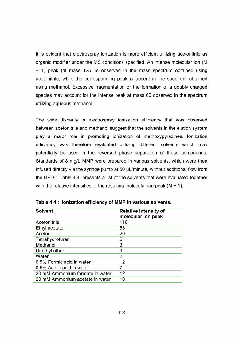
128

It is evident that electrospray ionization is more efficient utilizing acetonitrile as

organic modifier under the MS conditions specified. An intense molecular ion (M

+ 1) peak (at mass 125) is observed in the mass spectrum obtained using

acetonitrile, while the corresponding peak is absent in the spectrum obtained

using methanol. Excessive fragmentation or the formation of a doubly charged

species may account for the intense peak at mass 60 observed in the spectrum

utilizing aqueous methanol.

The wide disparity in electrospray ionization efficiency that was observed

between acetonitrile and methanol suggest that the solvents in the elution system

play a major role in promoting ionization of methoxypyrazines. Ionization

efficiency was therefore evaluated utilizing different solvents which may

potentially be used in the reversed phase separation of these compounds.

Standards of 8 mg/L MMP were prepared in various solvents, which were then

infused directly via the syringe pump at 50 µL/minute, without additional flow from

the HPLC. Table 4.4. presents a list of the solvents that were evaluated together

with the relative intensities of the resulting molecular ion peak (M + 1).

Table 4.4.: Ionization efficiency of MMP in various solvents.

Solvent Relative intensity of molecular ion peak

Acetonitrile 116 Ethyl acetate 53 Acetone 20 Tetrahydrofuran 5 Methanol 3 Di-ethyl ether 3 Water 2 0.5% Formic acid in water 12 0.5% Acetic acid in water 7 20 mM Ammonium formate in water 12 20 mM Ammonium acetate in water 10

129

Of the solvents evaluated, ionization of MMP is most efficient in acetonitrile.

Further optimization experiments therefore focussed on acetonitrile as the

organic mobile phase modifier utilized in conjunction with electrospray ionization.

4.3.4.2. The effect of the aqueous content of the mobile phase on ionization efficiency

As demonstrated earlier, the 3-alkyl-2-methoxypyrazines under investigation may

be separated efficiently utilizing reversed phase chromatography. The selected

separation involves gradient elution where the aqueous fraction of the mobile

phase is varied from 50% to 5% during the chromatographic run. The effect of

the varying aqueous content of the mobile phase on the ionization efficiency

utilizing ESI was evaluated by acquiring MS scan data while increasing the

aqueous content of the mobile phase. The response measured for mass 125 (3-

methyl-2-methoxypyrazine) at various mobile phase compositions is shown in

Figure 4.7.

130

0

2

4

6

8

10

12

80 85 90 95 100 105

Acetonitrile (%)

Inte

nsity

(x 1

000

000

)

Figure 4.7.: Intensity of M + 1 peak of MMP obtained with (positive mode) ESI at various mobile phase compositions of acetonitrile and water (100%, 99%, 95%, 90% and 85% acetonitrile respectively).

The ionization efficiency decreased when increasing the aqueous content of the

mobile phase above 5%. It was observed that in 85% aqueous acetonitrile, the

molecular ion peak (M + 1) is completely absent from the relevant spectrum.

4.3.4.3. The use of a volatile buffer to promote ionization

As protonation of the compound of interest is a premise for efficient positive

mode electrospray ionization, the use of formic acid to promote ionization was

investigated.

For this investigation, sample introduction was by direct infusion of a standard of

3 mg/L at 5 µL/minute via a syringe pump, in conjunction with a flow of 1

131

mL/minute from the liquid chromatograph. The quaternary solvent delivery

system was utilized to produce mobile phase compositions of varying acetonitrile,

water and formic acid content. The relative intensity of the molecular ion at each

mobile phase composition was obtained from the relevant mass spectra. Initial

investigations were performed using 3-methyl-2-methoxypyrazine, as this

compound is relatively weakly retained in the reversed phase separation and

hence elutes in mobile phase with a relatively high aqueous content. Figure 4.8.

presents the relative intensities of the molecular ion (M + 1, m/z = 125) at each

mobile phase composition for 3 mg/L MMP.

0

5

10

15

20

25

30

35

40

45

0 2 4 6 8 10 12Formic acid added (%)

Rela

tive

resp

onse 50%

60%70%80%90%95%

Figure 4.8.: ESI Ionization efficiency of MMP in mobile phase compositions ranging from 50% to 95% acetonitrile and 0% to 11% formic acid.

The addition of formic acid to the mobile phase affected an increase in the

ionization efficiency across the entire range of mobile phase compositions

evaluated. The optimal amount of formic acid decreases as the fraction of

acetonitrile in the mobile phase increases, while ionization efficiency increases

with the acetonitrile content of the mobile phase (as observed previously). The

132

most intense signal was observed using a mobile phase consisting of 90%

acetonitrile with 2% formic acid.

As optimal ionization efficiency was obtained between 80 and 90% acetonitrile

with between 2 and 4% formic acid, additional experiments were performed in

this range of mobile phase compositions. 3-Isobutyl-2-methoxypyrazine is the

most significant congener in Sauvignon blanc wine and is expected to elute with

the other major 3-alkyl-2-methoxypyrazines, IPMP and SBMP, at higher organic

modifier content of the mobile phase. Subsequent experiments were therefore

aimed at optimizing ionization of this compound. Figure 4.9. presents the relative

intensities of the molecular ion (M + 1, m/z = 167) at intermediate mobile phase

compositions for 6 mg/L IBMP infused at 5 µL/minute.

0

10

20

30

40

50

60

0 2 4 6 8 10Formic acid added (%)

Rel

ativ

e re

spon

se 80%83%86%89%92%

Figure 4.9.: ESI Ionization efficiency of IBMP in mobile phase compositions ranging from 80% to 92% acetonitrile and 0% to 8% formic acid.

It was found that optimal ionization of IBMP was obtained between 86% and 92%

acetonitrile with the addition of 1% formic acid. Further experiments at mobile

phase compositions of between 85 and 90% acetonitrile with 1% added formic

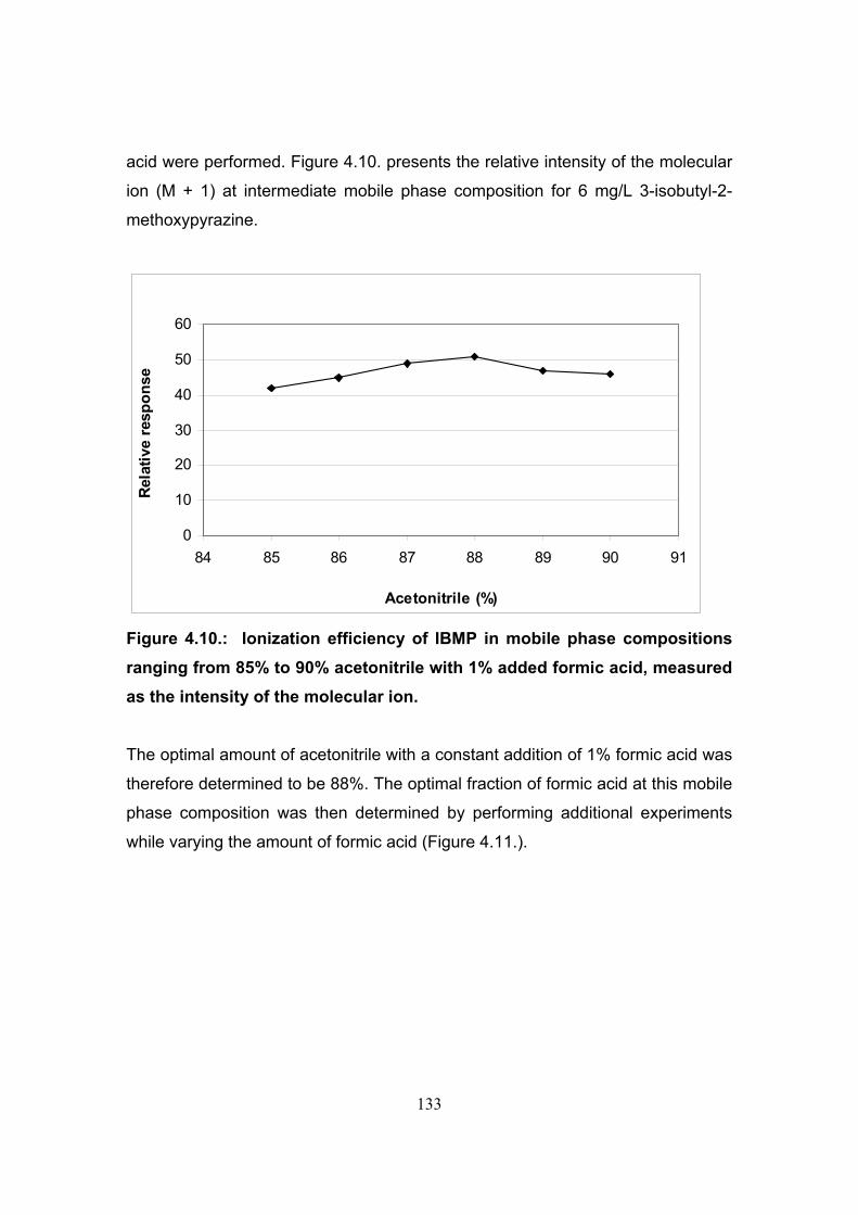
133

acid were performed. Figure 4.10. presents the relative intensity of the molecular

ion (M + 1) at intermediate mobile phase composition for 6 mg/L 3-isobutyl-2-

methoxypyrazine.

0

10

20

30

40

50

60

84 85 86 87 88 89 90 91

Acetonitrile (%)

Rel

ativ

e re

spon

se

Figure 4.10.: Ionization efficiency of IBMP in mobile phase compositions ranging from 85% to 90% acetonitrile with 1% added formic acid, measured as the intensity of the molecular ion.

The optimal amount of acetonitrile with a constant addition of 1% formic acid was

therefore determined to be 88%. The optimal fraction of formic acid at this mobile

phase composition was then determined by performing additional experiments

while varying the amount of formic acid (Figure 4.11.).

134

0

10

20

30

40

50

60

0 0.2 0.4 0.6 0.8 1 1.2 1.4 1.6

Formic acid (%)

Rela

tive

resp

onse

Figure 4.11.: Ionization efficiency of IBMP in mobile phase compositions ranging from 0.25% to 1.50% formic acid in 88% aqueous acetonitrile.

Electrospray ionization was therefore found to be optimal in a mobile phase

consisting of 1% formic acid in 88% acetonitrile. The variation in ionization

efficiency observed may be rationalized by considering that at the relatively high

flow-rates used (1 mL/minute), evaporation was more efficient in a mobile phase

that contains a relatively high proportion of volatile organic modifier. The increase

in efficiency with addition of formic acid that was observed may possibly be

ascribed to enhanced conductivity of the mobile phase and more efficient

protonation of the analyte at lower mobile phase pH.

4.3.4.4. The effect of mobile phase flow-rate on ionization efficiency

The effect of mobile phase flow-rate on the electrospray ionization efficiency was

evaluated by infusing a standard via the syringe pump at 5 µL/minute while

varying the flow from the liquid chromatograph between 0.1 and 1.0 mL/minute.

A 6 mg/L standard of IBMP was infused together with a mobile phase

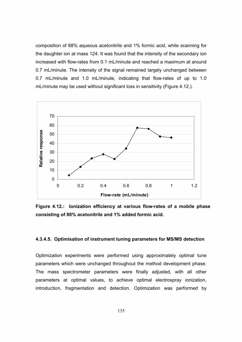
135

composition of 88% aqueous acetonitrile and 1% formic acid, while scanning for

the daughter ion at mass 124. It was found that the intensity of the secondary ion

increased with flow-rates from 0.1 mL/minute and reached a maximum at around

0.7 mL/minute. The intensity of the signal remained largely unchanged between

0.7 mL/minute and 1.0 mL/minute, indicating that flow-rates of up to 1.0

mL/minute may be used without significant loss in sensitivity (Figure 4.12.).

0

10

20

30

40

50

60

70

0 0.2 0.4 0.6 0.8 1 1.2

Flow-rate (mL/minute)

Rela

tive

resp

onse

Figure 4.12.: Ionization efficiency at various flow-rates of a mobile phase consisting of 88% acetonitrile and 1% added formic acid.

4.3.4.5. Optimisation of instrument tuning parameters for MS/MS detection

Optimization experiments were performed using approximately optimal tune

parameters which were unchanged throughout the method development phase.

The mass spectrometer parameters were finally adjusted, with all other

parameters at optimal values, to achieve optimal electrospray ionization,

introduction, fragmentation and detection. Optimization was performed by

136

infusing a standard (6 mg/L) of IBMP at 3 µL/minute via a syringe pump, in

conjunction with a flow of 1.0 mL/minute from the liquid chromatograph at the

mobile phase composition of 88% acetonitrile with 1% formic acid. Various

parameters were optimized by observing the intensity of the relevant ions while

adjusting each parameter to produce the best sensitivity. Tables 4.5. and 4.6.

presents the optimized instrument tuning parameters determined in this manner.6

Table 4.5.: Optimized ESI tuning parameters for MS/MS operation determined for mobile phase of 88% acetonitrile with 1% added formic acid.

Parameter Value Source: Positive mode electrospray ionization Capillary (kV) 2.2 Cone (V) 34 Extractor (V) 6.00 RF Lens (V) 0.1 Source Temperature (°C) 120 Desolvation Temperature (°C) 350 Cone Gas Flow (L/Hr) 50 Desolvation Gas Flow (L/Hr) 650 Analyzer LM 1 Resolution 10.0 HM 1 Resolution 10.0 Ion Energy 1 0.3 Entrance -5 Collision (eV) 18 Exit 0 LM 2 Resolution 14.0 HM 2 Resolution 14.0 Ion Energy 2 1.0 Multiplier (V) 700 Collision Gas Flow (L/Hr) 0.40

The parameters for the MRM transitions were optimized by infusing a standard of

3 mg/L of the five components in conjunction with a mobile phase flow of 1

mL/minute from the HPLC. The mobile phase was 88% aqueous acetonitrile with

1% added formic acid. Experimental parameters were adjusted to produce

optimal response for the components of interest. The inter channel delay time

was 0.020 seconds while the inter scan time was 0.100 seconds.

137

Table 4.6.: Optimized parameters for MRM transitions.

Compound Parent Ion (Da)

Daughter Ion (Da)

Transition Cone (V)

Collision (eV)

MMP 125.0 56.2 2 ° 34 20 125.0 97.0 1 ° 34 14 EMP 139.0 83.0 2 ° 34 16 139.0 124.0 1 ° 34 18 IPMP 152.9 83.0 3 ° 34 16 152.9 122.9 2 ° 34 26 152.9 137.9 1 ° 34 18 IBMP 167.0 97.0 2 ° 34 20 167.0 125.0 1 ° 34 16 SBMP 167.0 123.0 2 ° 34 24 167.0 138.0 1 ° 34 18

4.3.5. Reversed phase separation of methoxypyrazines using optimized electrospray ionization conditions

As the sample extracts are expected to contain relatively large amounts of

potentially interfering matrix elements (especially considering the concentration

factor associated with the proposed sample preparation procedure),

chromatographic separation is essential to separate the majority of the matrix

elements from the peaks of interest. An optimized separation would involve

gradient elution starting with a high aqueous fraction in the mobile phase. To

compensate for the quenching effect of water experienced by early eluting peaks,

the initial fraction of formic acid should correspondingly be increased. The three

major wine methoxypyrazines, IPMP, IBMP and SBMP, are however strongly

retained and may efficiently be eluted in 88% acetonitrile, where ionization

efficiency is optimal. Alternatively, all five components may be determined with

maximum efficiency by isocratic elution using the optimal mobile phase

composition. As the mobile phase in the proposed isocratic separation contains a

relatively high organic fraction, the reduced viscosity of the mobile phase

provides the option to use longer columns to increase the separation efficiency.

138

Two possible strategies for the reversed phase separation of the components of

interest were therefore identified for evaluation. These comprised gradient elution

of the components of interest with post-column addition of optimized amounts of

formic acid and isocratic elution at a mobile phase composition where

electrospray ionization of the components of interest is optimal.

4.3.5.1. Gradient elution with post-column addition of optimized amounts of formic acid

The proportion of formic acid required to optimize electrospray ionization is

relatively high and varies from approximately more than 10% in 50% aqueous

acetonitrile to 2% in 95% aqueous acetonitrile. The relatively high amount of

formic acid required in this range of mobile phase compositions precludes the

use of the liquid chromatography system for its introduction as the silica-based

analytical column can only tolerate a mobile phase pH of between 2 and 8.8 The

application of a gradient for the separation therefore demands that the required

formic acid be added independently, via post-column addition. Formic acid was

introduced via post-column addition utilizing a second LC system employing a

time-programmed flow gradient to produce an optimal mobile phase composition

throughout the separation. A relay switch on the primary separation system was

used to synchronize the two LC systems. A pulse damper was utilized with the

secondary liquid chromatography system, in an effort to produce pulse-free,

consistent delivery of the post-column reagent.

The C18 column described in section 4.2.2. was used to perform the separation.

The gradient used in the separation was as follows: 50% acetonitrile initially,

increased to 90% acetonitrile in 5 minutes (via a concave curve), followed by

90% acetonitrile for 10 minutes, at a constant flow-rate of 0.4 mL/minute. Post-

column addition of formic acid was done isocratically, by adding a 50% solution

139

in acetonitrile, via a flow-controlled gradient as follows: Starting at 0.1 mL/minute

for 10.5 minutes, changing to 0.02 mL/minute in 30 seconds followed by 0.02

mL/minute for 3.5 minutes. The column temperature was 40°C for these

experiments.

The method described above produced efficient separation of the components of

interest. It was however found that the variation in peak area between injections

was relatively large, with a relative standard deviation of approximately 20%. As

the amount of formic acid in the mobile phase significantly affects the ionization

efficiency, especially at relatively high aqueous compositions, small variations in

the addition of formic acid to the mobile phase are expected to significantly affect

the measured peak areas. It may reasonably be assumed that post-column

addition of reagents would be more precise if the secondary system was used at

higher flow-rates (due to pump limitations at these low flow-rates), but the

addition of the post-column reagent was deliberately minimized to reduce the

resulting peak-broadening.

140

Figure 4.13.: Gradient reversed phase separation of a standard containing 20 pg MMP, EMP, IPMP and SBMP and 80 pg IBMP with post-column addition of optimized amounts of formic acid, ESI ionization.

Gradient separation as described produced efficient separation (Figure 4.13.) of

the components of interest but as reproducibility of the results was poor the

performance of the method was regarded as inadequate. Optimal method

efficiency could not be realized utilizing gradient elution.

4.3.5.2. Isocratic elution at the optimal mobile phase composition

The optimal mobile phase composition for electrospray ionization of IBMP was

determined to be 88% aqueous acetonitrile with 1% added formic acid. The pH of

this solution is approximately 2.6, which is high enough for routine utilization with

silica-based stationary phases. Isocratic reversed phase separation of the

Time0.00 2.00 4.00 6.00 8.00 10.00 12.00 14.00 16.00

%

IBMP

IPMP

EMP

MMP

SBMP

141

components of interest with this mobile phase composition was therefore

investigated.

As the composition of the mobile phase is dictated by the ionization efficiency,

the only chromatographic parameter available for manipulation to achieve

optimal separation (with the selected phase) is the efficiency, determined by the

column length (and particle size). The column had a diameter of 4.6 mm with 3

µm particle size, the flow-rate was therefore maintained at 1.0 mL/minute while

the column-oven temperature was kept at 40°C. Optimization experiments

therefore basically reduced to the determination of the longest effective column

that can be used at optimal conditions without generation of excessive back-

pressure.

It was determined that a column of effective length of 300 mm produced efficient

resolution of the components of interest. When operated with the specified

mobile phase composition at 1.0 mL/minute and at 40°C, the back-pressure on

the system did not exceed 152 bar. (The pressure limit of the column is 240 bar.)

142

Figure 4.14.: Isocratic reversed phase separation of a standard containing 20 pg MMP, EMP, IPMP and SBMP and 80 pg IBMP, 300 mm C18 column (88% aqueous acetonitrile, 1% added formic acid), ESI ionization.

Isocratic elution utilizing an optimized mobile phase composition (88%

acetonitrile, 1% formic acid) produced the highest ionization efficiency for all

components of interest. Approximate detection limits were in the order of 0.1 pg

on column for all five components. The reproducibility of results was good while

the use of a column with effective length of 300 mm resulted in adequate

resolution for all components. The six-port valve was utilized to divert the column

effluent to waste prior to elution of the components of interest as well as

thereafter. The effluent flow was switched to the detector only when the

components of interest eluted to avoid fouling of the source with non-volatile

sample matrix.

Time0.00 1.00 2.00 3.00 4.00 5.00 6.00 7.00 8.00

%

IBMP

IPMP

EMPMMP

SBMP

143

Isocratic elution, as described in this section, was therefore considered to be the

most efficient mode of separation to be utilized in conjunction with electrospray

ionization.

4.3.6. Method specificity utilizing isocratic reversed phase separation and electrospray ionization

A preliminary evaluation of method specificity revealed that the analyte response

was attenuated by co-eluting matrix elements of the sample extract. It was

concluded that electrospray ionization of the analyte are suppressed in the

presence of concentrated matrix elements present in the extracts.

Chromatographic separation, as described in paragraph 4.3.5.1. and 4.3.5.2.,

failed to resolve the analyte sufficiently from the interfering sample matrix to

produce an unattenuated signal. Subsequent clean-up of the extracts with mixed

mode reversed phase SPE, as described in Chapter 3 (3.3.4.2.2.), in

combination with isocratic as well as gradient separation, similarly failed to

resolve the interferons to affect levels of efficiency comparable to that obtained

with the standards. ESI is not universally applicable to all analytes that can be

ionized and it is widely accepted that some analytes are incompatible with this

source.4 Atmospheric pressure chemical ionization (APCI) is known to be less

susceptible to matrix effects and was therefore subsequently evaluated for the

analysis of 3-alkyl-2-methoxypyrazines in wine.

4.3.7. Atmospheric pressure chemical ionization

APCI was provisionally determined to be free from quenching effects caused by

the sample matrix and was therefore optimized for possible utilization in the

determination of methoxypyrazines in concentrated wine extracts. APCI can also

144

tolerate relatively high flow-rates and are therefore compatible with the use of 4.6

mm diameter separation columns operated at optimum flow-rates.5

4.3.8. Efficiency of atmospheric pressure chemical ionization in various elution systems utilized in reversed phase separations

The efficiency of APCI was evaluated in elution systems of aqueous acetonitrile

and methanol. Sample introduction was by direct loop injections of a standard to

produce 80 pg of analyte on column, with a mobile phase flow of 0.75 mL/minute.

The quaternary pump was utilized to produce various mobile phase compositions

starting from 50% organic phase and increasing to 98% in 10% increments. A

constant composition of 1% formic acid was used in each of these mobile

phases, as this was found to provide optimal ionization efficiency in ESI. The

MRM transitions indicated previously for ESI were used to evaluate the effect of

the mobile phase composition. The results are summarized in Figure 4.15.

0

20

40

60

80

100

40 60 80 100

Mobile phase composition (%)

Rel

ativ

e re

spon

se

AcetonitrileMethanol

Figure 4.15.: APCI ionization efficiency of IBMP in acetonitrile- and methanol based mobile phases, with 1% formic acid.

145

APCI efficiency in the aqueous methanol system (1% formic acid) was found to

produce higher sensitivity (above 60% organic phase).

Protonation of the target species is a premise for efficient positive mode APCI,

and as a volatile acidic modifier was found to significantly affect ESI ionization

efficiency, the amount of formic acid in the mobile phase was further optimized

for APCI. Sample introduction and detection was performed as outlined above

while mobile phase compositions ranged from 0 to 2% formic acid in 90%

aqueous methanol and acetonitrile respectively. The results for the MRM

acquisitions for IBMP are summarized in Figure 4.16.

0

20

40

60

80

100

0 0.5 1 1.5 2 2.5

Added formic acid (%)

Rela

tive

resp

onse

AcetonitrileMethanol

Figure 4.16.: Ionization efficiency in 90% aqueous acetonitrile and methanol mobile phases with various amounts of added formic acid.

Formic acid, added to an effective concentration of 0.5% was found to be optimal

in both mobile phase systems. The improvement in ionization efficiency realized

with the use of added formic acid (up to 2%) was insignificant, utilization of this

reagent was therefore suspend. It is also evident that ionization in aqueous

146

methanol is more efficient throughout the range investigated, and methanol was

therefore selected as the organic modifier in the reversed phase separations

performed with APCI.

4.3.9. Effect of the orientation of the APCI probe on ionization efficiency

In the APCI interface, the mobile phase stream enters the probe where it is

pneumatically converted to an aerosol, which is then rapidly dried and converted

to the gas phase. The position of the probe may be adjusted parallel to the axis

running through the ion optics and the pinhole entrance to the mass

spectrometer. The effect of this adjustment is to orientate the spray optimally

relative to the corona discharge needle and the sampling cone. The position of

the spray relative to the corona discharge needle and the sampling cone is

critical for the respective processes of ionization and ion transfer. The source is

equipped with a vernier probe adjuster to facilitate precise positioning of the tip.

Figure 4.17.: APCI source illustrating the position of the probe, corona needle and sampling orifice.

Probe

Sampling orifice

Corona needle

147

The effect of probe orientation on the APCI efficiency was evaluated by making

repeated direct loop injections of a standard to produce 80 pg of analyte on

column in conjunction with a mobile phase flow of 0.75 mL/minute, while

adjusting the probe through the range of possible settings. MRM transition

signals were used to observe the effect of the probe orientation. As the position

of the APCI probe was found to have a significant effect on the efficiency, further

experiments were also carried out at intermediate vernier settings (240 pg on

column) thus refining the optimal probe position. The results for IBMP in the

range of possible probe orientations are presented in Figure 4.18.

0

10

20

30

40

50

60

0 5 10 15

Vernier setting

Rel

ativ

e re

spon

se

Coarse adjustmentFine adjustment

Figure 4.18.: Effect of probe orientation on ionization efficiency of IBMP. Optimized ionization and introduction of ions is achieved when the effluent spray

is directed approximately at the mid-point between the corona discharge needle

and the sample cone. The vernier setting corresponding to the best signal was

6.5.

148

4.3.10. Effect of mobile phase flow-rate on ionization efficiency

The effect of mobile phase flow-rate on APCI ionization efficiency was evaluated

by observing the intensity of the signal obtained while varying the flow from the

liquid chromatograph between 0.2 and 1.1 mL/minute. The mobile phase

composition was 90% methanol with 1% formic acid. The response for IBMP as a

function of flow-rate is presented below (Figure 4.19.).

0

1020

30

40

5060

70

80

0 0.2 0.4 0.6 0.8 1 1.2

Flow rate (mL/minute)

Rel

ativ

e re

spon

se

Figure 4.19.: APCI ionization efficiency of IBMP at various mobile phase flow-rates.

From these data it can be concluded that the efficiency essentially increases with

flow rate across the studied range. Higher flow-rates appears to enhance the

efficiency, a phenomenon that that may be explained by the fact that in APCI

analyte molecules are ionized by interaction with ionized solvent molecules so

that at higher flow-rates more interactions, and hence higher efficiencies, are

possible.4 This suggests that a 4.6 mm diameter analytical separation column

and flow rates close to or at the optimal flow rate of 1.0 mL/minute may be used

in the current application.

149

4.3.11. Optimisation of APCI source parameters

The corona discharge current may have a significant effect on sensitivity and

depends upon the polarity of the compound as well as the analytical mobile

phase.9 The optimal corona discharge current was determined utilizing the same

protocol as before and observing the effect of the corona discharge current on

the intensity of the signals obtained (Figure 4.20.). A corona discharge current of

4.4 μA was found to provide the best signal response and was therefore used in

subsequent experiments.

0

10

20

30

40

50

60

70

80

0 2 4 6 8 10 12Discharge current (uA)

Rela

tive

resp

onse

Figure 4.20.: APCI ionization efficiency at various corona discharge currents.

Inside the APCI probe, the eluent stream emerging from the fused silica capillary

is converted to an aerosol spray of fine droplets. The nebulizer plume is then

rapidly heated in a stream of nitrogen gas to ensure that it leaves the probe as a

stream of desolvated sample droplets. The support gas controls the droplet

residence time and allows the sample to be swept from the probe efficiently.9

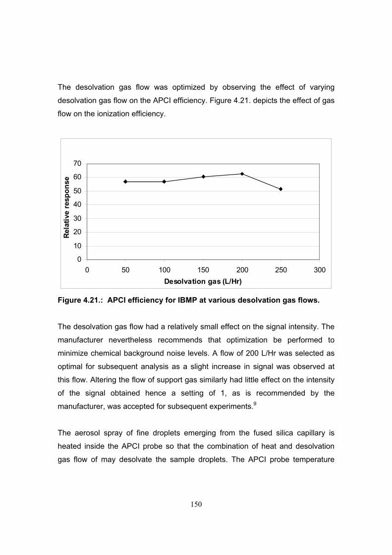
150

The desolvation gas flow was optimized by observing the effect of varying

desolvation gas flow on the APCI efficiency. Figure 4.21. depicts the effect of gas

flow on the ionization efficiency.

0

10

20

30

40

50

60

70

0 50 100 150 200 250 300Desolvation gas (L/Hr)

Rela

tive

resp

onse

Figure 4.21.: APCI efficiency for IBMP at various desolvation gas flows.

The desolvation gas flow had a relatively small effect on the signal intensity. The

manufacturer nevertheless recommends that optimization be performed to

minimize chemical background noise levels. A flow of 200 L/Hr was selected as

optimal for subsequent analysis as a slight increase in signal was observed at

this flow. Altering the flow of support gas similarly had little effect on the intensity

of the signal obtained hence a setting of 1, as is recommended by the

manufacturer, was accepted for subsequent experiments.9

The aerosol spray of fine droplets emerging from the fused silica capillary is

heated inside the APCI probe so that the combination of heat and desolvation

gas flow of may desolvate the sample droplets. The APCI probe temperature

151

may be controlled to ensure efficient desolvation of the analyte droplets without

possible thermal decomposition of the target species.9

The probe temperature was optimized by observing the intensity of signals

obtained for different desolvation temperatures while maintaining the desolvation

gas flow at the previously determined optimal value of 200 L/hour.

0

20

40

60

80

100

0 100 200 300 400 500 600 700Desolvation temperature ( °C)

Rel

ativ

e re

spon

se

Figure 4.22.: APCI efficiency of IBMP at various desolvation temperatures at a desolvation gas-flow of 200 L/hour.

A desolvation temperature of 200°C was determined to be optimal (Figure 4.22.).

The maximum desolvation temperature recommended for operation of the APCI

probe is 650°C.9 The observed optimal temperature is therefore relatively low, a

phenomenon that may be ascribed to the fact that the analyte molecules are

relatively volatile and that the eluting mobile phase is similarly volatile. Optimal

efficiency may therefore simply be achieved at relatively low desolvation

temperatures.

152

4.3.12. Optimisation of instrument tuning parameters for MS-MS operation

For optimal quantitative MRM analysis, the MS tuning parameters were adjusted

to achieve the highest sensitivity for each analyte. Tuning was performed by

infusing 5 mg/L standards of the methoxypyrazines under investigation at 15

µL/minute via a syringe pump, in conjunction with a flow of 1.0 mL/minute from

the liquid chromatograph, at the mobile phase composition encountered in the

separation (80% aqueous methanol). The parameters were optimized by

observing the intensity of the relevant ions while experimental parameters were

adjusted (Table 4.7.). The inter channel delay time and the inter scan time was

0.020 seconds and 0.100 seconds respectively.

Table 4.7.: Tuning parameters for APCI MS-MS operation.

Parameter Value Source: IonSABRE APCI source, positive mode Corona (µA) 4.4 Cone (V) 34 Extractor (V) 6.00 RF Lens (V) 0 Source Temperature (°C) 150 Desolvation Temperature (°C) 200 Cone Gas Flow (L/Hr) 50 Desolvation Gas Flow (L/Hr) 200 Analyzer LM 1 Resolution 10.0 HM 1 Resolution 10.0 Ion Energy 1 0.3 Entrance -5 Collision (eV) 18 Exit 0 LM 2 Resolution 14.0 HM 2 Resolution 14.0 Ion Energy 2 1.0 Multiplier (V) 700 Collision Gas Flow (L/Hr) 0.35

153

Table 4.8.: MRM transitions used.


Daughter Ion (Da)

Transition Cone (V)

Collision (eV)

MMP 125.0 56.2 2 ° 34 20 125.0 97.0 1 ° 34 14 EMP 139.0 111.0 2 ° 34 16 139.0 123.9 1 ° 34 18 IPMP 152.9 122.9 2 ° 34 26 152.9 137.9 1 ° 34 18 IBMP 167.0 124.0 2 ° 34 22 167.0 125.0 1 ° 34 16 SBMP 167.0 123.0 2 ° 34 24 167.0 138.0 1 ° 34 18

The fragmentation patterns observed for the ion transitions listed in Table 4.8.

correspond mainly to cleavage of the alkyl side-chain at the alkyl-substituted

carbon atoms. The observed cleavage of the branched alkyl side-chains are due

to charge stabilization at the position of branching. Generally the largest

substituent at a branch is eliminated most readily (SBMP, 167 > 138). In alkyl-

substituted aromatic compounds, cleavage is also very probable at the bond β to

the ring (IPMP, IBMP and SBMP). The aromatic ring stabilizes resulting cationic

daughter ion by charge delocatization.10 The relevant mass spectra obtained are

attached as Appendix 1. Table 4.9. presents accurate mass information and

proposed molecular formulae pertaining to the molecular ions and daughter ion

fragments listed in Table 4.8. Accurate mass determinations were performed

utilizing the Q-TOF instrument specified in the experimental section (4.2.2.). The

integrity of the data is evident from the close correlation between the observed

and theoretical masses obtained for the relevant molecular ions (M + 1).

Furthermore it can be noted that the observed masses of the primary and

secondary daughter ions correlate very well with the theoretical masses of the

proposed molecular formulae indicating a high degree of confidence in the

proposed elemental compositions of these secondary ions.

154

Table 4.9.: Accurate mass information and molecular formulae pertaining to ion transitions of interest.

Compound M + 1 Observed mass (Theoretical mass) (Da)

Daughter 1 Observed mass (Da)

Elemental composition (Theoretical mass) (Da)

Daughter 2 Observed mass (Da)

Elemental composition (Theoretical mass) (Da)

MMP 125.0721 (125.0715)

97.0765 C4H5N2O (97.0402)

56.0497 C2H2NO (56.0136)

EMP 139.0873 (139.0871)

124.0656 C6H8N2O (124.0637)

111.0910 C5H7N2O (111.0558)

IPMP 153.1028 (153.1004)

138.0806 C7H10N2O (138.0793)

123.0567 C6H7N2O (123.0558)

IBMP 167.1184 (167.1160)

125.0714 C6H9N2O (125.0715)

124.0639 C6H8N2O (124.0637)

SBMP 167.1180 (167.1160)

138.0783 C7H10N2O (138.0793)

123.0572 C6H7N2O (123.0558)

4.3.13. Method specificity utilizing separation on a C18 column and atmospheric pressure chemical ionization

A preliminary evaluation of method specificity revealed that the analyte response

for IBMP and SBMP was not affected by the matrix of the extracts and that the

peaks of interest were sufficiently resolved from interferences. An unknown

interfering compound, with identical molar mass and daughter ions, was however

found to co-elute with IPMP. Co-elution was evident from the fact that the ion

ratio for the two transitions were not consistent with that obtained for the

calibration standards. Identification of the interferon was attempted utilizing off-

line GC-MS and LC-TOF analysis of collected fractions but was unsuccessful.

Lacey et al. reported similarly that matrix elements interfered with the

determination of IPMP in Sauvignon blanc wines with GC-MS.11 Separation of

the interferon from IPMP was attempted by additional optimization of the solvent

gradient. Changes in the solvent gradient failed to achieve separation of the

interferon from IPMP. As IPMP is, after IBMP, probably the most abundant 3-

alkyl-2-methoxypyrazine in Sauvignon blanc wine11, the relevant quantitative

155

information may be essential in the characterization of the methoxypyrazine

profile of the cultivar and detection of adulteration of the wine. It is therefore

imperative that this compound be separated from interferences so that it may be

quantified successfully.

Figure 4.23.: Standard of MMP (68.4 pg), EMP (65.9 pg), IPMP (61.5 pg), IBMP (238.4 pg) and SBMP (60.4 pg), separated on C18 column.

Time 5.00 10.00 15.00 20.00

%

0

5.00 10.00 15.00 20.00

%

0

5.00 10.00 15.00 20.00

%

0

5.00 10.00 15.00 20.00

%

0

5.00 10.00 15.00 20.00

%

0

SBMP

IBMP

IPMP

EMP

MMP

156

Figure 4.24.: Sample extract separated on C18 column showing co-eluting compounds.

Three separate strategies were then evaluated for resolution of IPMP from the

interferon, namely SPE clean-up of the extract, utilization of alternative column

chemistries to achieve sufficient selectivity to affect separation and online sample

clean-up and separation utilizing a secondary column in tandem with the primary

separation column.

Time 5.00 10.00 15.00 20.00

%

0

5.00 10.00 15.00 20.00

%

0

5.00 10.00 15.00 20.00

%

0

5.00 10.00 15.00 20.00

%

0

5.00 10.00 15.00 20.00

%

0

SBMP

IBMP

Interferonco-elutingwith IPMP

Interferon co-eluting with EMP

MMP not detected

157

4.3.13.1. SPE clean-up of extracts for reversed phase separation on a C18 column

Sample clean-up utilizing Oasis mixed mechanisms SPE in combination with

distillation and solvent extraction, as described in Chapter 3 (3.3.4.2.2.), was

evaluated to remove the interfering compound co-eluting with IPMP. Oasis SPE

cartridges contain a sorbent that is a copolymer composed of divinylbenzene and

N-vinylpyrrolidone units and is designed to have a hydrophilic-lipophilic balance

when used under reversed phase conditions. This procedure was optimized to

enhance retention of basic compounds and it was hoped that an alternative

selectivity would be achieved with this method so that the interferon might be

removed. It was however found that the co-eluting interferon persisted upon

separation of the purified extract on a C18 column. Quantification of IPMP was

therefore not possible utilizing this method with additional SPE sample clean-up.

4.3.13.2. Evaluation of alternative column chemistries to achieve improved selectivity for the reversed phase separation of the 3-alkyl-2-methoxypyrazines

Alternative reversed phase column chemistries were evaluated for the separation

of sample extracts to ensure resolution of analytes from interfering matrix

elements. These experiments were also aimed at identifying column chemistries

that may be utilized in tandem for on-line sample clean-up and separation,

described in the following section. Additional column chemistries that were

evaluated were phenyl-hexyl, C8, C5 and cyano (column details in Table 4.1.).

It was observed that the phenyl-hexyl as well as the C8 columns provided

separation of the three major 3-alkyl-2-methoxypyrazines (IPMP, IBMP and

SBMP) from major matrix interferences. However, major matrix interferences co-

eluted with the minor 3-alkyl-2-methoxypyrazines (MMP and EMP). The phenyl-

158

hexyl column produced stronger retention of the analytes which afforded elution

with a mobile phase containing a relatively high fraction of volatile organic

solvent. The gradient used for elution of the analytes from the phenyl-hexyl

phase afforded elution of the major 3-alkyl-2-meyhoxypyrazines in a mobile

phase consisting of approximately 80% methanol, while similar elution on the C8

phase was achieved in approximately 70% methanol. The advantages of eluting

the analytes in a mobile phase that contains a relatively high fraction of volatile

solvent are more efficient solvent removal in the ionization source and hence

better sensitivity as well as potential separation from interferences, as discussed

earlier.

4.3.13.3. Online clean-up of extracts utilizing a secondary column in tandem with the primary separation column

The LC-MS system incorporates a six-port valve that enables the system to be

configured for sample injection on one column (preparative or secondary column)

followed by time-programmable switching of the effluent to the main separation

(or primary) column. A premise for successful reversed phase on-line sample

clean-up and separation utilizing a secondary column in tandem with the primary

separation column, is that the organic content of the eluting mobile phase on the

secondary column must not exceed that of the starting mobile phase on the

primary separation column, to facilitate concentration of the solute at the head of

this column. The preferred column combination for such a strategy would

therefore require that the compounds of interest be eluted from the secondary

column utilizing a mobile phase that has a relatively high aqueous content while

separation on the primary column is achieved with a mobile phase with high

organic content. The cyano column (50 x 4.6 mm, 5 μm) was selected as the

secondary column and phenyl-hexyl (250 x 4.6 mm, 5 μm) as the primary

separation column, as they are relatively polar and apolar respectively and

correspondingly required low and high organic content of the mobile phase for

159

elution of the compounds of interest. It is also expected that relatively apolar

interferences may efficiently be removed from the analytes by separation on the

relatively polar secondary column. Separation on the apolar primary column may

then possibly be free from strongly retained interferences that co-elute with the

substances under investigation.

The separation was performed as follows: The sample extract was injected on

the secondary column and the effluent diverted to waste. The solvent program

started at 5% methanol, constant for 1 minute, increasing to 40% methanol in 7

minutes via a linear gradient followed by 40% methanol for 1 minute. At 7

minutes the effluent was switched from waste to the primary separation column.

At 8 minutes the methanol content was increased linearly from 40% to 90% in 12

minutes. After 1 minute, the methanol content was decreased to 15%

(equilibration of primary separation column). The effluent was diverted to waste

at run-time 26 minutes upon which the secondary column was equilibrated at 5%

methanol for 1.5 minutes, for a total run-time of 27.5 minutes. The flow was

constant throughout the separation at 1.0 mL/minute and the column-oven

temperature was controlled at 40°C. The maximum pressure did not exceed 160

bar.

It was found that separation on the two-column system described affected

separation of the major interferences from IPMP. Co-eluting matrix elements

were however still found to interfere with the determination of the minor 3-alkyl-2-

methoxypyrazines (MMP and EMP). Figure 4.25. presents a chromatogram

obtained for a standard that was separated utilizing the described method. It can

also be noted that MMP is not detected at this concentration. This compound

eluted in a relatively aqueous mobile phase, and ionization parameters

(especially desolvation temperature of 200°C) was optimized for ionization of

methoxypyrazines in mobile phases that contains a higher organic content.

Ionization efficiency in the relatively aqueous phase was therefore not optimal

and may account for the absence of MMP from the chromatogram.

160

Time5.00 10.00 15.00 20.00

%

9

5.00 10.00 15.00 20.00

%

1

5.00 10.00 15.00 20.00

%

2

5.00 10.00 15.00 20.00

%

1

5.00 10.00 15.00 20.00

%

1

SB

MP

IBM

PIP

MP

EM

P

Time5.00 10.00 15.00 20.00

%

9

5.00 10.00 15.00 20.00

%

1

5.00 10.00 15.00 20.00

%

Time5.00 10.00 15.00 20.00

%

9

5.00 10.00 15.00 20.00

%

1

5.00 10.00 15.00 20.00

%

2

5.00 10.00 15.00 20.00

%

1

5.00 10.00 15.00 20.00

%

1

2

5.00 10.00 15.00 20.00

%

1

5.00 10.00 15.00 20.00

%

1

SB

MP

SB

MP

IBM

PIB

MP

IPM

PIP

MP

EM

PE

MP

Figure 4.25.: Chromatogram of standard solution containing 13.7 pg MMP, 13.2 pg EMP, 12.3 pg IPMP, 47.6 pg IBMP and 12.1 pg SBMP. Reversed phase separation utilizing CN functionalized secondary column in tandem with Ph-hexyl primary separation column.

4.3.14. LC-APCI-MS analysis of methoxypyrazines in wine

In summary, it was shown that APCI is more efficient utilizing methanol as the

mobile phase organic modifier, and that ionization efficiency generally increases

161

with methanol content and the addition of formic acid (up to 1%). Since optimal

sensitivity depends on the amount of methanol in the mobile phase, the

chromatographic separations of methoxypyrazines were optimized to achieve

separation via gradient elution in order to ensure elution of the target analytes

with a methanol-rich mobile phase. As the addition of formic acid affected a

relatively small increase in efficiency it was not used in the method due to the

effect it may have on the longer term stability of the silica-based separation

columns utilized. The two-column system as well as the phenyl-hexyl column

affected resolution of the three important 3-alkyl-2-methoxypyrazines (IPMP,

IBMP and SBMP) from most major matrix interferences. It was finally decided

that the phenyl-hexyl phase provides the highest efficiency for separation of the

sample extracts and as the procedure is relatively uncomplicated compared to

the former, it was accepted for utilization in the investigation. A preliminary

evaluation of method specificity revealed the analyte response was not affected

by the matrix of the extracts and that the peaks of interest were sufficiently

resolved from major interferences (Figure 4.27.). The two minor 3-alkyl-2-

methoxypyrazines, MMP and EMP, were however completely obscured by

unresolved matrix elements. Matrix interference was observed to be more

problematic with the said congeners for two reasons. Firstly they have lower

molecular ion-and daughter-ion masses, interfering ions were therefore possibly

more common. Secondly these were also retained less strongly by the stationary

phase not only resulting in elution in a region of the chromatogram where most of

the sample matrix is expected, but also eluting in a relatively aqueous fraction of

the mobile phase, thereby reducing their detectability. As these compounds were

also expected to have very low concentrations and are not known to be present

or to play a role in the odor of the cultivar, they were excluded from the

investigation. The focus was therefore exclusively on the major 3-alkyl-2-

methoxypyrazines (IPMP, IBMP and SBMP) from this point onwards.

As separation of closely eluting compounds is critical in this application, the

efficiency of the designated column must be optimal. The column dimensions

162

was limited to 250 x 4.6 mm with particle size of 5 µm to achieve high relative

efficiency (longer column) while limiting the backpressure (larger particle size)

resulting from separation via a methanol and water gradient. The optimized

gradient separation utilizing the phenyl-hexyl phase was as follows: The gradient

started at 35% methanol, increased (linearly) to 85% methanol in 18 minutes

followed by column clean-up at 95% methanol for 2.5 minutes. The flow was

maintained at 1.0 mL/minute throughout and re-equilibration time was 3.5

minutes. The column temperature was maintained at 40°C and the total run-time

was 25 minutes while the divert valve was used to direct the effluent to the

detector only between time 14 and 18 minutes, the rest going to waste. Figure

4.26. and 4.27. represents MRM chromatograms obtained for a standard and

wine extract utilizing separation on this phase (only primary ion transitions

shown).

163

Figure 4.26: Chromatogram of a standard containing 61.6 pg IPMP, 238.4 pg IBMP and 60.4 pg SBMP. Gradient separation on phenyl-hexyl column.

Time5.00 10.00 15.00 20.00

%

0

5.00 10.00 15.00 20.00

%

0

5.00 10.00 15.00 20.00

%

0

SBMP

IBMP

IPMP

164

Figure 4.27: Chromatogram of a Sauvignon blanc wine extract, separated on a phenyl-hexyl column using the optimized separation conditions (100 µL injected). Extract prepared as described in experimental section (concentration factor 500). Interferon separated from IPMP peak.

4.4. Conclusions

Electrospray ionization was utilized initially for ionization of five 3-alkyl-2-

methoxypyrazines. The mobile phase and tuning parameters were optimized

Time 5.00 10.00 15.00 20.00

%

0

5.00 10.00 15.00 20.00

%

0

5.00 10.00 15.00 20.00

%

0

SBMP

IBMP

Interferon

IPMP

165

using standards and relatively high efficiencies were obtained. It was however

subsequently found that the matrix of the wine extracts caused severe quenching

of the ionization and that no form of additional sample clean-up, separation or

tuning could resolve this defect.

ESI generally requires low mobile phase flow-rates.4 The manufacturer of the

system claims that flow-rates of up to 1.0 mL/minute may be accommodated but

that typical values ranging between 0.1 and 0.2 mL/minute are preffered.6 It has

however been reported that (low) flow-rate may be critical for efficient ESI

(depending on various factors including instrument design) and it is possible that

the flow-rate utilized with ESI in this investigation (1.0 mL/minute) was too high

and that this contributed to the quenching effects that were experienced in the

presence of the wine matrix.12 The flow-rate used (1.0 mL/minute) was optimal

for the 4.6 mm diameter separation columns while flow splitting was not

considered due to the sensitivity requirements of the method. The larger

diameter columns (4.6 mm) were utilized as opposed to that of 2.1 mm as the

former provides larger loading capacity8, a critical factor for efficient separation of

concentrated extracts via large injection volumes. It was also determined that

with standards, the efficiency of ESI did not decrease with flow-rates between 0.2

and 0.7 mL/minute and that it was relatively unchanged between 0.7 and 1.0

mL/minute. With real samples containing extremely concentrated matrices, the

flow-rate requirements for optimal ionization efficiency might have been different

from those attainable with standards.

Atmospheric pressure chemical ionization was then optimized for use with the

reversed phase separation method utilizing a C18 phase. Sensitivity obtained

with APCI was approximately an order of magnitude lower than with ESI but

ionization of the analytes were unaffected by the wine sample matrix. It was then

found that unknown matrix components co-eluted with IPMP as well as MMP and

EMP. Separation selectivity was improved by utilizing a phenyl-hexyl separation

phase to resolve IPMP while MMP and EMP was omitted from the investigation.

166

In conclusion, ESI and APCI were evaluated for the trace-level analysis of 3-

alkyl-2-methoxypyrazines in wine. ESI is more efficient, but was not suitable due

to matrix effects. APCI avoided this problem, and an optimized method for the

analysis of the three major wine 3-alkyl-2-methoxypyrazines was developed

which produced good performance. This optimized APCI method with separation

on a phenyl-hexyl phase was subsequently validated (Chapter 5) for the

determination of three 3-alkyl-2-methoxypyrazines (IPMP, IBMP and SBMP) in

South African Sauvignon blanc wine.

167

REFERENCES

(1) D. A. Skoog, F. J. Holler, T. A. Nieman, PRINCIPLES OF

INSTRUMENTAL ANALYSIS, 5th ed.(1998), Saunders College

Publishing, Philadelphia, 660 - 724.

(2) Sigma Chemicals, P.O. Box 10434, Aston Manor, 1630, South Africa.

(3) L.G. Wade Jr., ORGANIC CHEMISTRY, 4th ed.(1999), Prentice-Hall inc.,

Upper Saddle River, New Jersey, 07458, 856 - 858.

(4) C. F. Poole, S. K. Poole, CHROMATOGRAPHY TODAY, (1991), Elsevier

Science Publishing Company Inc., 655 Avenue of the Americas, New

York, NY 10010, U.S.A.

(5) M. C. McMaster, LC/MS A PRACTICAL USER’S GUIDE, (2005), John

Wiley & Sons Inc., 111 River Street, Hoboken, NJ 07030, 51 - 84. (6) WATERS MICROMASS QUATTRO PREMIER XE MASS

SPECTROMETER OPERATOR’S GUIDE, Waters Corporation, 34 Maple

street, MA 01757, U.S.A.

(7) D. R. Lide, CRC HANDBOOK OF CHEMISTRY AND PHYSICS, 86th

ed.(2006 – 2006), CRC Press, 6000 Broken Sound Parkway NW, Suite

300, Boca Raton FL.

(8) Phenomenex, 411 Madrid ave., Torrance, CA, 90501-1430, U.S.A.

(9) IonSABRE APCI USER’S GUIDE, Waters Corporation, 34 Maple Street,

Milford, MA 01757, U.S.A.

(10) R. M. Silverstein, G. C. Bassler, T. C. Morrill, SPECTROMETRIC

IDENTIFICATION OF ORGANIC COMPOUNDS, 5th ed., John Wiley &

Sons Inc, 3 - 44. (11) M. J. Lacey, M. S. Allen, R. L. N. Harris, W. V. Brown,


Am. J. Enol. Vitic., 42 (1991), 103 – 108.

(12) G. J. van Berkel, V. Kertesz, USING THE ELECTROCHEMISTRY OF

THE ELECTROSPRAY ION SOURCE, Analytical Chemistry, (2007), 5510

- 5520.

168

CHAPTER 5

Validation of the optimized RP-LC-APCI-MS method for the analysis of 3-alkyl-2-methoxypyrazines in wine


The objective of this study is in the first instance to quantify selected 3-alkyl-2-

methoxypyrazines in South African Sauvignon blanc wine and secondly to use

the information to characterize authentic wine in this regard. In this Chapter the

performance characteristics of the analytical method developed previously will be

validated to illustrate that the method is capable of producing the required

quantitative analytical data.

5.2. Materials and methods

5.2.1. Chemicals and samples

Acetonitrile, dichloromethane and tannic acid were from Merck (Darmstadt,

Germany), IBMP, IPMP, SBMP, methanol and ethanol from Aldrich (Sigma-

Aldrich, South Africa) and formic acid from Associated Chemical Enterprises

(ACE, South Africa).


on an analytical balance followed by dilution utilizing A-grade volumetric


standards were prepared in 10% ethanol.

169

Wine samples for the recovery study were prepared by mixing together at

random, various bottled Sauvignon blanc wines to establish batches of at least 5

L. Aliquots of each batch were then transferred to 1 L volumetric flasks, to which

appropriate amounts of standard were added and finally made up to the mark

with wine, to produce series of fortified wine samples. Each series of wine

samples thus consisted of unfortified wine as well as fortified wine (three levels of

fortification: 1, 10 and 100 ng/L).

5.2.2. Sample preparation

Aliquots of wine samples were transferred to an A-grade 500 mL volumetric flask

up to the mark. The contents of the flask were then transferred quantitatively to a

1 L boiling flask by repeated rinsing with water. After a single glass ball and

spatula tip of tannic acid were added, the sample was distilled utilizing a 60 cm

fractionating column, continuing distillation until 100 mL of distillate was

collected. The distillate was cooled in a two-stage process, first passing through

a water-cooled condenser followed by passage through a slurry of ice and water

before collection in a 100 mL volumetric flask. The distillate was then transferred

quantitatively to a 500 mL separating funnel, containing a 35 mm egg-shaped

magnet, by repeated rinsing with water. The distillate was then extracted with

three portions (10 mL, 5 mL and 5 mL) of dichloromethane by rapid stirring for 10

minutes at a time. The combined dichloromethane fractions were transferred to a

pear-shaped vessel with a 1.5 mL graduated stem, to which 0.5 mL of

concentrated formic acid was added previously. The dichloromethane extracts

were evaporated at room temperature under a stream of nitrogen gas until less

than 0.5 mL of concentrate remained. Finally the extract was reconstituted to 1

mL utilizing a solution of 40% acetonitrile in water, homogenized and transferred

to a 1.8 mL amber vial for analysis.

170

5.2.3. Chromatographic details

The LC-MS system utilized was a Waters Alliance 2695 liquid chromatograph

(Waters Corporation, Milford, U.S.A.) with Waters Micromass Quattro Premier XE

tandem quadrupole mass spectrometric detector (Manchester, U.K.). The

concentrated sample extracts were separated by reversed phase liquid

chromatography utilizing a methanol and water gradient and a phenyl hexyl

separation column (Phenomenex Luna, 250 x 4.6 mm, 3µm) thermostatted at

40°C. The gradient started at 35% methanol, increased to 85% in 18 minutes,

followed by a column clean-up step consisting of 95% methanol for 2.5 minutes.

The flow was maintained at 1.0 mL/minute throughout the separation and re-

equilibration time was 3.5 minutes. Variable injection volumes were used ranging

from 5 to 100 µL. Components of interest were introduced into the mass

spectrometer utilizing atmospheric pressure chemical ionization (positive ion

mode). The mass spectrometer was operated in multiple reaction monitoring

(MRM) mode, the experimental parameters are given in Chapter 4 (Table 4.7.

and 4.8.).


5.3.1. Minimum method criteria

Limited quantitative data available for 3-alkyl-2-methoxypyrazines in South

African Sauvignon blanc wines indicate levels of IBMP in the range of < 1 to 14

ng/L.1 Although no corresponding information pertaining to the other major 3-

alkyl-2-methoxypyrazines, IPMP and SBMP, are available in the literature, these

are expected to be at levels not exceeding approximately 10 to 20% of the total

3-alkyl-2-methoxypyrazines in Sauvignon blanc wine.2 A comparable study

involving a number of Sauvignon blanc wines of Australian, New Zealand and

French origin, produced the following results:2

171

Table 5.3.: Methoxypyrazine levels in some Australian, New Zealand and French Sauvignon blanc wines.2

Methoxypyrazine Levels (ng/L) IPMP 0.9 to 5.6 IBMP 0.6 to 38.1 SBMP 0.1 to 1.0

It should be noted that the limit of detection of the analytical method used in this

study was 0.15 ng/L and that IPMP and SBMP were not detected in some of the

wines. The methoxypyrazine levels in New Zealand wines were also significantly

(and consistently) higher than in Australian wines, a phenomenon ascribed to the

fact that fruit grown under cool conditions generally produces higher

methoxypyrazine levels.2,3,4

In order to characterize the profile of abundance of 3-alkyl-2-methoxypyrazines in

South African Sauvignon blanc, the analytical method should at least be capable

of accurate determination of the three important methoxypyrazines namely IPMP,

IBMP and SBMP. Method detection levels in the order of 0.03 ng/L and minimum

quantification levels in the order of 0.10 ng/L may be considered minimum

requirements in terms of sensitivity for the purpose of this study. The method

accuracy, expressed as recovery, should be better than 80%. As a single 750 mL

bottle is available per sample and 500 mL of wine is consumed in the sample

preparation procedure, the precision of the method must be such that reliable

results may be produced from a single determination per sample. The intra-assay

precision, expressed as the RSD of the recovery, should therefore be better than

10%.

172

5.3.2. Determination of the linear working range

A linearity study utilizing standards was performed to demonstrate linear system

response over the range of expected residue levels. Quantities ranging from

extinction levels to 4000 pg on column were injected, which corresponded to a

maximum sample residue level of 80 ng/L, a concentration factor of 500 and a

100 µL injection. The mass of analyte injected was plotted against measured

peak area as well as response factor (peak area/mass). The results of the

linearity study are summarized in Tables 5.4. to 5.6.

Table 5.4.: Linearity, IPMP primary and secondary ion transitions (152.9 to 137.9 and 122.9 respectively).

Mass (pg)

Average peak area /% RSD (n = 3, 152.9 > 137.9)

Response factor (area / mass)



0.6150 15 / 74% 24 32 / 46% 52 1.230 47 / 58% 38 63 / 14% 51 2.460 55 / 55% 22 81 / 43% 33 6.150 161 / 16% 26 150 / 26% 24 24.60 873 / 9% 35 768 / 12% 31 123.0 3937 / 4% 32 3545 / 1% 29 369.0 11940 / 4% 32 10446 / 3% 28 1230 40482 / 5% 33 36899 / 6% 30

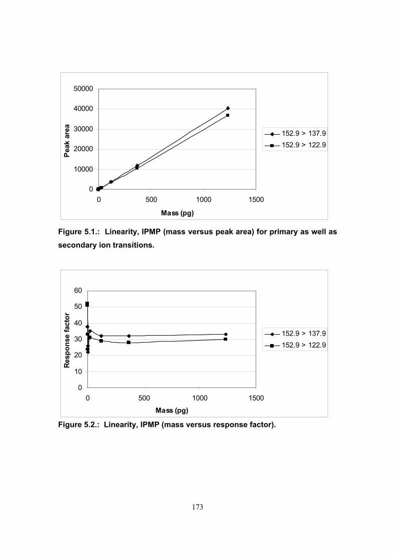
173

0

10000

20000

30000

40000

50000

0 500 1000 1500

Mass (pg)

Pea

k ar

ea 152.9 > 137.9152.9 > 122.9

Figure 5.1.: Linearity, IPMP (mass versus peak area) for primary as well as secondary ion transitions.

0

10

20

30

40

50

60

0 500 1000 1500

Mass (pg)

Resp

onse

fact

or

152.9 > 137.9152.9 > 122.9

Figure 5.2.: Linearity, IPMP (mass versus response factor).

174

Table 5.5.: Linearity, IBMP primary and secondary ion transitions (167.0 to 125.0 and 124.0 respectively).

Mass (pg)





2.384 110 / 32% 46 70 / 29% 29 4.768 280 / 15% 59 186 / 19% 39 9.536 582 / 17% 61 405 / 7% 42 23.84 1456 / 8% 61 1152 / 5% 48 95.36 6434 / 3% 67 4753 / 4% 50 476.8 29483 / 1% 62 21028 / 1% 44 1430 93214 / 1% 65 67438 / 1% 47 4768 306207 / 4% 64 224342 / 4% 47

0

50000

100000

150000

200000

250000

300000

350000

0 1000 2000 3000 4000 5000 6000Mass (pg)

Pea

k ar

ea 167.0 > 125.0167.0 > 124.0

Figure 5.3.: Linearity, IBMP (mass versus peak area).

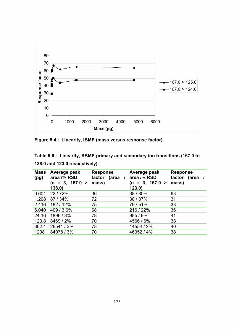
175

0

10

20

30

40

50

60

70

80

0 1000 2000 3000 4000 5000 6000Mass (pg)

Resp

onse

fact

or

167.0 > 125.0167.0 > 124.0

Figure 5.4.: Linearity, IBMP (mass versus response factor).

Table 5.6.: Linearity, SBMP primary and secondary ion transitions (167.0 to 138.0 and 123.0 respectively).

Mass (pg)





0.604 22 / 72% 36 38 / 80% 63 1.208 87 / 34% 72 38 / 37% 31 2.416 182 / 12% 75 79 / 51% 33 6.040 409 / 3.6% 68 216 / 22% 36 24.16 1896 / 3% 78 985 / 9% 41 120.8 8469 / 2% 70 4566 / 6% 38 362.4 26541 / 3% 73 14554 / 2% 40 1208 84078 / 3% 70 46052 / 4% 38

176

0

15000

30000

45000

60000

75000

90000

0 500 1000 1500Mass (pg)

Peak

Are

a

167.0 > 138.0167.0 > 123.0

Figure 5.5.: Linearity, SBMP (mass versus peak area).

0

15

30

45

60

75

90

0 500 1000 1500Mass (pg)

Res

pons

e fa

ctor

167.0 > 138.0167.0 > 123.0

Figure 5.6.: Linearity, SBMP (mass versus response factor).

The Pearson’s correlation coefficients5, r, were determined from the limit of

quantification (5 pg) to highest injected masses in each case and were as follows

Table 5.7.:

177

Table 5.7.: Pearson’s correlation coefficients for the calibration curves of the compounds of interest.

Compound IPMP IBMP SBMP Primary transition 0.99998 0.99998 0.99987 Secondary transition 0.99985 0.99998 0.99987

The system response was found to be linear between the quantification limit and

4 000 pg and 1000 pg on-column for IBMP, and IPMP and SBMP respectively.

Quantification of the said compounds should therefore strictly be performed

within this mass range. When actual samples are analyzed, the system may be

calibrated over a smaller concentration range which is better suited to the

determination of the substances under investigation at realistic sample

concentrations. Where the sample concentration exceeds the established

working range, appropriate injection volumes should be used to ensure that the

mass injected falls within the actual calibration range.

5.3.3. Limits of detection and quantitation

The limits of detection (MDL) and of quantitation (MQL) of the method for the

substances under investigation were obtained from the linearity study. These

values were estimated based on the smallest amount of solute that produced a

signal equivalent to three times and ten times of the average noise, respectively.

The data processing software (Masslynx 4.0) was used to calculate the signal-to-

noise ratios using unsmoothed chromatograms for each of the MRM signals. At

the minimum quantifiable level, the ratios of all ions used for identification and

quantitation were found to be consistent with those produced at higher

concentrations (Table 5.9.). Measured minimum detectable quantities obtained

correspond to sample residue levels of 0.03 ng/L, while the minimum

quantification limits correspond to levels of 0.10 ng/L, considering sample pre-

concentration of a factor of 500 and injection volumes of 100 µL.

178

Table 5.8.: Minimum detectable and quantifiable levels obtained with the method.

Methoxypyrazine MDL (pg on column) MQL (pg on column) IPMP 1.5 5.0 IBMP 1.5 5.0 SBMP 1.5 5.0

Time5.00 10.00 15.00 20.00

%

5.00 10.00 15.00 20.00

%

5.00 10.00 15.00 20.00

%

SB

MP

IBM

PIP

MP

Time5.00 10.00 15.00 20.00

%

5.00 10.00 15.00 20.00

%

5.00 10.00 15.00 20.00

%

Time5.00 10.00 15.00 20.00

%

5.00 10.00 15.00 20.00

%

5.00 10.00 15.00 20.00

%

SB

MP

SB

MP

IBM

PIP

MP

Figure 5.7.: Chromatogram of a standard solution containing the three 3-alkyl-2-methoxypyrazines under investigation close to the limit of quantitation. IPMP = 6.2 pg, IBMP = 23.8 pg, SBMP = 6.0 pg.

179

5.3.4. Method specificity

The three target methoxypyrazines were identified utilizing retention times as well

as the ratios of abundance measured for the relevant primary- and secondary

ions. Table 5.9. presents the relevant data used for peak identification (obtained

from calibration standards).

Table 5.9.: Criteria for peak identification.

Methoxypyrazine Retention time (minutes)

Primary transition

Secondary transition

Ratio of ions

IPMP 15.39 152.9 > 137.9 152.9 > 122.9 1.11 IBMP 16.81 167.0 > 125.0 167.0 > 124.0 1.37 SBMP 17.21 167.0 > 138.0 167.0 > 123.0 1.88

Some European Union guidelines for compound identification by MS/MS require

that a precursor parent ion together with two daughter ions (and one ion ratio) be

obtained for confirmatory purposes. The relative daughter ion intensities,

expressed as a percentage of the intensity of the most intense ion, must be

consistent with that of the reference standards (at comparable concentrations).

The relevant retention times obtained for the analytes in the sample should also

match those of the reference standards. The maximum allowable tolerance

regarding the ion ratios is approximately ± 20% while retention times should

correlate within 2.5%.6

The compounds of interest, determined in wine samples (unfortified wine as well

as fortified to 1, 10 and 100 ng/L) as part of the recovery study, produced

retention time and ion ratio values (Table 5.10.) that were consistent with the

identification criteria outlined above. These criteria (Table 5.9.) were therefore

also applied for compound identification in this study.

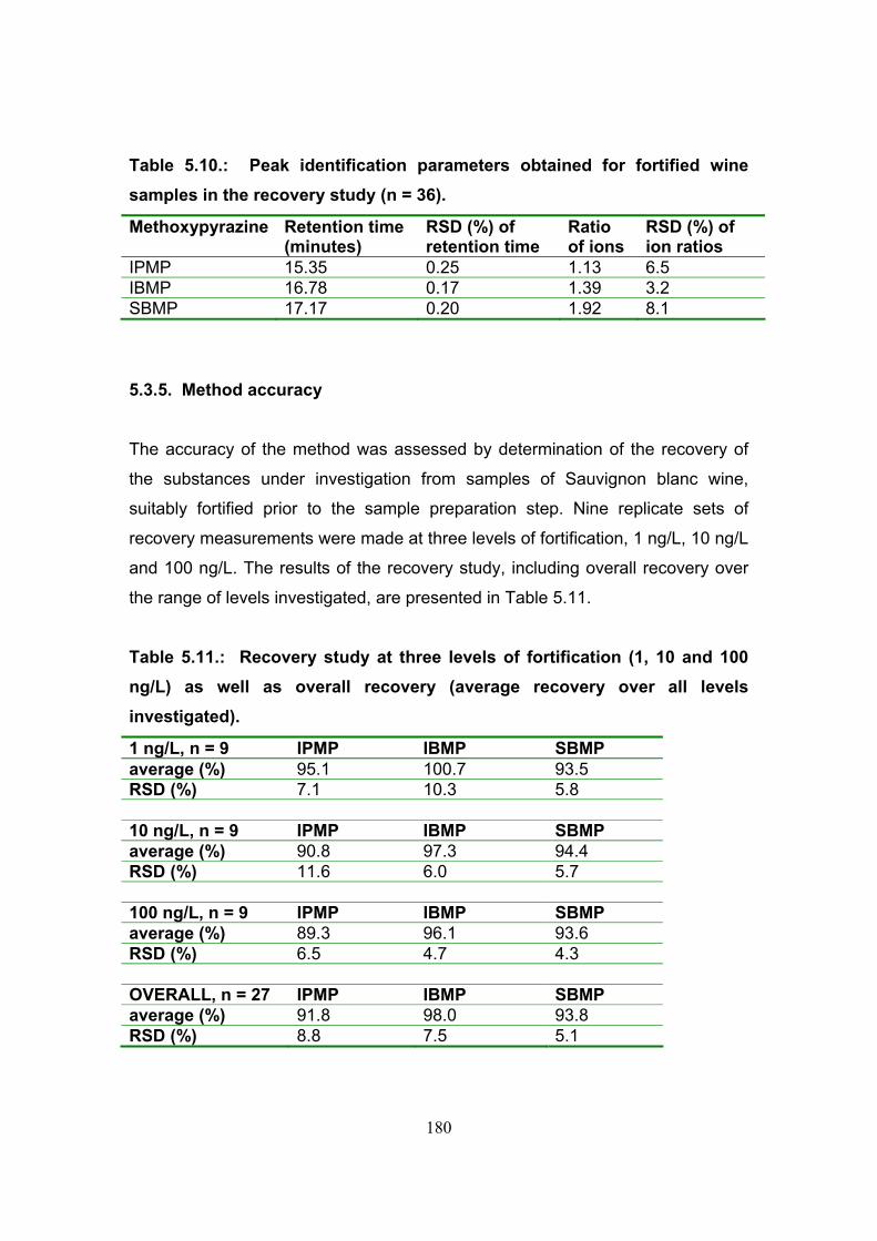
180

Table 5.10.: Peak identification parameters obtained for fortified wine samples in the recovery study (n = 36).

Methoxypyrazine Retention time (minutes)

RSD (%) of retention time

Ratio of ions

RSD (%) of ion ratios

IPMP 15.35 0.25 1.13 6.5 IBMP 16.78 0.17 1.39 3.2 SBMP 17.17 0.20 1.92 8.1

5.3.5. Method accuracy

The accuracy of the method was assessed by determination of the recovery of

the substances under investigation from samples of Sauvignon blanc wine,

suitably fortified prior to the sample preparation step. Nine replicate sets of

recovery measurements were made at three levels of fortification, 1 ng/L, 10 ng/L

and 100 ng/L. The results of the recovery study, including overall recovery over

the range of levels investigated, are presented in Table 5.11.

Table 5.11.: Recovery study at three levels of fortification (1, 10 and 100 ng/L) as well as overall recovery (average recovery over all levels investigated).

1 ng/L, n = 9 IPMP IBMP SBMP average (%) 95.1 100.7 93.5 RSD (%) 7.1 10.3 5.8 10 ng/L, n = 9 IPMP IBMP SBMP average (%) 90.8 97.3 94.4 RSD (%) 11.6 6.0 5.7 100 ng/L, n = 9 IPMP IBMP SBMP average (%) 89.3 96.1 93.6 RSD (%) 6.5 4.7 4.3 OVERALL, n = 27 IPMP IBMP SBMP average (%) 91.8 98.0 93.8 RSD (%) 8.8 7.5 5.1

181

5.3.6. Method precision

The reproducibility of the LC-MS instrument was determined by performing

repeated injections of a standard solution containing the three methoxypyrazines.

Reproducibility was expressed as the standard deviation of the peak area

obtained for the components of interest (Table 5.12.).

Table 5.12.: Instrument precision obtained for the LC-MS system upon injection of a standard (n = 7).

IPMP (61.5 pg) IBMP (238.4 pg) SBMP (60.4 pg) average 2181 15699 4404 RSD (%) 2.9 1.5 4.3

The intra-assay precision was assessed by considering the repeatability obtained

in the recovery study. The recovery of the substances under investigation was

better than 90% with RSD of less that 10% at concentrations of 1 ng/L, 10 ng/L

and 100 ng/L.

5.3.7. Uncertainty of measurements and reporting of results

The uncertainty of measurements associated with the procedure was estimated

by calculating the range of the 95% confidence interval (C.I.) about the

measurements performed in the recovery study (i.e. at levels of 1 ng/L, 10 ng/L

and 100 ng/L). The confidence limits (C.L.) pertaining to the recovery of the

target species were calculated using the following equation:7

95% C.L. = mean value ± zs / (n)1/2

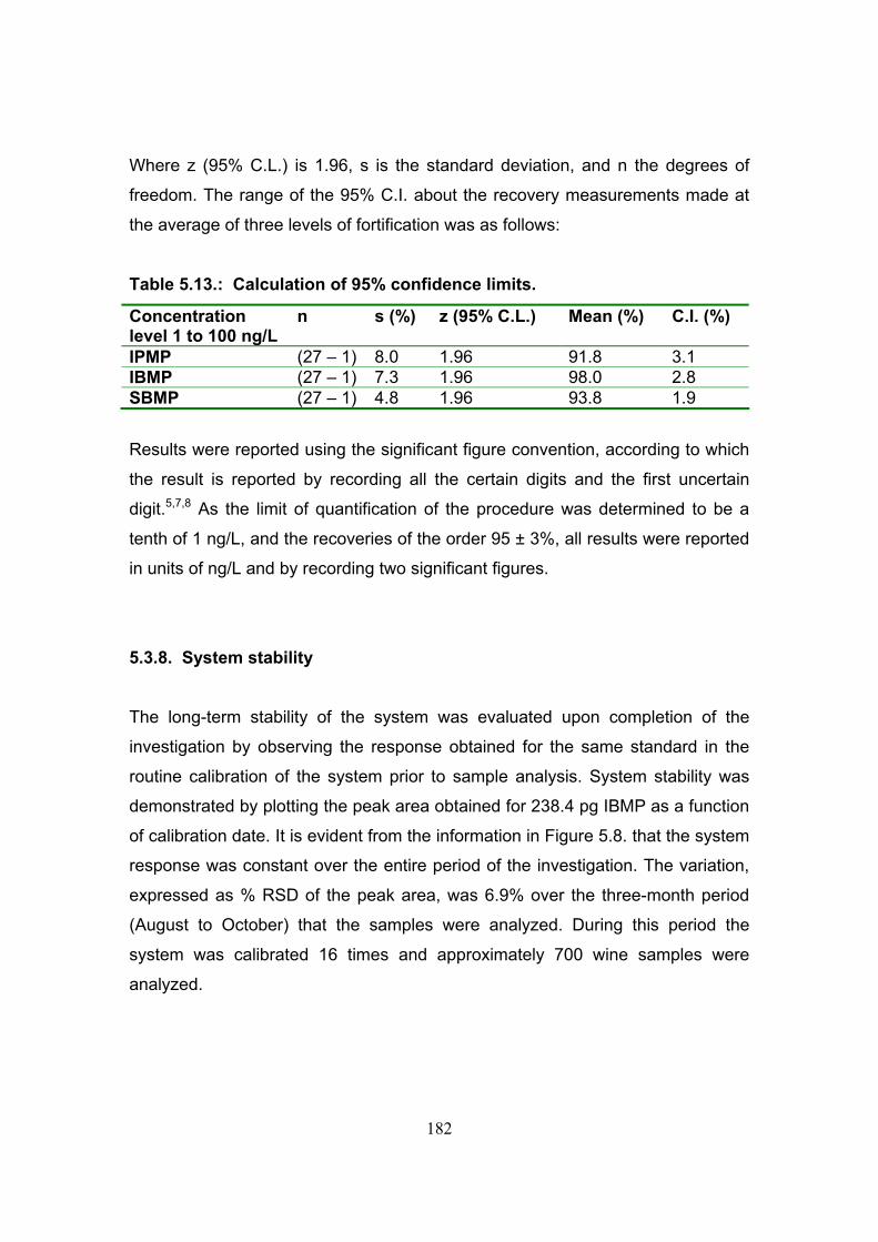
182

Where z (95% C.L.) is 1.96, s is the standard deviation, and n the degrees of

freedom. The range of the 95% C.I. about the recovery measurements made at

the average of three levels of fortification was as follows:

Table 5.13.: Calculation of 95% confidence limits.

Concentration level 1 to 100 ng/L

n s (%) z (95% C.L.) Mean (%) C.I. (%)

IPMP (27 – 1) 8.0 1.96 91.8 3.1 IBMP (27 – 1) 7.3 1.96 98.0 2.8 SBMP (27 – 1) 4.8 1.96 93.8 1.9

Results were reported using the significant figure convention, according to which

the result is reported by recording all the certain digits and the first uncertain

digit.5,7,8 As the limit of quantification of the procedure was determined to be a

tenth of 1 ng/L, and the recoveries of the order 95 ± 3%, all results were reported

in units of ng/L and by recording two significant figures.

5.3.8. System stability

The long-term stability of the system was evaluated upon completion of the

investigation by observing the response obtained for the same standard in the

routine calibration of the system prior to sample analysis. System stability was

demonstrated by plotting the peak area obtained for 238.4 pg IBMP as a function

of calibration date. It is evident from the information in Figure 5.8. that the system

response was constant over the entire period of the investigation. The variation,

expressed as % RSD of the peak area, was 6.9% over the three-month period

(August to October) that the samples were analyzed. During this period the

system was calibrated 16 times and approximately 700 wine samples were

analyzed.

183

0

5

10

15

20

3 Aug

6 Aug

14 Aug

16 Aug

21 Aug

22 Aug

29 Aug

5 Sep

t

12 Sep

t

20 Sep

t

27 Sep

t3 O

ct9 O

ct

16 O

ct

17 O

ct

29 O

ct

Calibration date

Peak

are

a x

1000

Figure 5.8.: System stability over the period of the investigation (August to October) expressed as the peak area of 238.4 pg IBMP on column.

5.4. Conclusions

The validation study revealed that the method met the minimum requirements as

outlined in section 5.3.1. and that it is therefore suitable for the routine trace level

determination of the said compounds in Sauvignon blanc wine.

The recoveries obtained indicate that the sample preparation procedure,

described in Chapter 3, produces precise (RSD less than 10%) pre-concentration

of the analytes with good recovery (better than 90%). The precision of the LC-

APCI-MS method was equally good (RSD less than 5%) while linear system

184

response was demonstrated from 5 to 4000 pg injected. The MDL and MQL for

the method were determined to be 0.03 and 0.10 ng/L respectively.

The performance characteristics of this LC-MS method were generally better

than that of all published GC methods utilized for the same purpose. The GC

methods produced MDL values ranging from 0.15 to 2 ng/L while MQL values in

the order of 2 ng/L were reported. These latter techniques are therefore at least

five times less sensitive than the described LC-MS method.

185

REFERENCES

(1) J. Marais, P. Minnaar, F. October, 2-METHOXY-3-

ISOBUTYLPYRAZINE LEVELS IN A SPECTRUM OF SOUTH AFRICAN

SAUVIGNON BLANC WINES, Wynboer, (2004).



Am. J. Enol. Vitic., 42 (1991), 103 – 108.

(3) M. S. Allen, M. J. Lacey, R. L. N. Harris, W. V. Brown, CONTRIBUTION

OF METHOXYPYRAZINES TO SAUVIGNON BLANC WINE AROMA,

Am. J. Enol. Vitic., 42 (1991), 109 - 112.

(4) K. Hashizume, T. Samuta, GRAPE MATURITY AND LIGHT

EXPOSURE AFFECT BERRY METHOXYPYRAZINE

CONCENTRATION, Am. J. Enol. Vitic., 50 (1999), 194 - 198.

(5) VOGEL’S TEXTBOOK OF QUANTITATIVE CHEMICAL ANALYSIS, 5 th

ed.(1991), Longman Scientific & Technical, Harlow, 127 - 149.

(6) M. J. O’Keeffe, S. Martin, L. Regan, VALIDATION OF A

MULTIRESIDUE LIQUID CHROMATOGRAPHY-TANDEM MASS

SPECTROMETRIC METHOD FOR THE QUANTITATION AND

CONFIRMATION OF CORTICOSTEROID RESIDUES IN URINE,

ACCORDING TO THE PROPOSED SANCO 1085 CRITERIA FOR

BANNED SUBSTANCES, Analytica Chimica Acta, 483 (2003), 341 -

350.

(7) D. A. Skoog, D. M. West, F. J. Holler, FUNDAMENTALS OF

ANALYTICAL CHEMISTRY, 7 th ed. (1996), Saunders College

Publishing, Orlando, 660 - 724.

(8) J. M. Miller, J. B. Crowther, ANALYTICAL CHEMISTRY IN A GMP

ENVIRONMENT, A PRACTICAL GUIDE, (2000), John Wiley & Sons

Inc., 605 Third Avenue, New York, NY 10158-0012, 77 - 103.

186

CHAPTER 6

The contents of some 3-alkyl-2-methoxypyrazines in South African Sauvignon blanc wine and detection of

adulteration


The overall objectives of this study were in the first instance to develop and

implement a method for the determination of 3-alkyl-2-methoxypyrazines in South

African Sauvignon blanc wine at their natural levels of occurrence and secondly

to analyze a spectrum of wines, representative of the South African Sauvignon

blanc industry. A comprehensive database of the 3-alkyl-2-methoxypyrazine

content of South African Sauvignon blanc wine may thus be established, and

used to implement a protocol for unequivocal identification of adulterated wines

regarding addition of foreign sources of 3-alkyl-2-methoxypyrazines.

Residues of the three major 3-alkyl-2-methoxypyrazines in South African

Sauvignon blanc wines were analyzed by liquid chromatography with mass

spectrometric detection. The method yielded qualitative (confirmatory)

information pertaining to the components of interest in addition to quantitative

information. Three 3-alkyl-2-methoxypyrazenes, 3-isobutyl-2-methoxypyrazine

(IBMP), 3-sec-butyl-2-methoxypyrazine (SBMP) and 3-isopropyl-2-

methoxypyrazine (IPMP) were thus investigated and quantified. The method

yielded limits of detection and quantification of 0.03 ng/L and 0.10 ng/L,

respectively.

Two parameters were identified that may be used to distinguish adulterated

wines. The IBMP concentration, despite showing considerable variance, was

187

confined to a range spanning approximately two orders of magnitude (0.40 to 44

ng/L). Possible maximum values for this compound in South African Sauvignon

blanc wines may therefore be established and classification of the wine according

to factors such as the region of origin and vintage attempted. Furthermore, it was

found that South African Sauvignon blanc wines contain the three analysed

pyrazenes in distinct relative amounts and that these ratios may therefore be

used to elucidate authenticity. In addition, the effect of adulteration with green

pepper extracts or synthetic flavor preparations on the relative abundances were

evaluated by characterizing the corresponding profiles in green pepper extracts

and synthetic flavor preparations. The analytes were also determined in

Sauvignon blanc vine leaves and in a small number of wines of other cultivars.

The data was analyzed utilizing multivariate and univariate statistical methods to

investigate possible grouping of samples in the dataset and to distinguish

adulterated wines. Principal component analysis (Statistica version 7 and 8) and

Anova (Statistica version 8) were used to perform data analysis. The results for

Anova are discussed concurrently with that of PCA.

6.2. Materials and methods

6.2.1. Samples

A total of 577 South African Sauvignon blanc wines, from all wine-producing

regions and of vintages 1999 to 2007, were analyzed. A number of wines

produced form other grape cultivars (roughly 6 per cultivar, recent vintages) were

also analyzed. Samples were obtained from submissions under the South African

controlled appellations system (South African Wine and Spirit Board) as well as

from export applications (South African National Department of Agriculture). Two

samples suspected to be adulterated with green pepper extracts or synthetic

preparations, were also confiscated earlier by the Department of Agriculture

188

under the provisions of the Liquor Products Act.1,2 In order to maintain

confidentiality, information pertaining to individual producers and estates are

omitted.

Green peppers were obtained from the local trade and were not purchased from

the same vendor or on the same date. The synthetic flavor preparations were

from The Duckworth Group (Killarney Gardens, South Africa) while Sauvignon

blanc vine leaves were obtained from the IWBT, Stellenbosch University.

Additional information pertaining to the chemical analysis of the Sauvignon blanc

wine samples were obtained from archived data that were used for certification of

the products under the South African controlled appellations system. Methods of

analysis used to obtain this data were as follows: Alcohol content by

densiometry, total reducing sugars by flow-injection analysis, total acidity by

titration and the pH was measured with a pH meter.

6.2.2. Sample preparation

Aliquots of wine samples (500 mL) were distilled (60 cm fractionating column)

followed by exhaustive liquid extraction with dichloromethane. The combined

dichloromethane fractions (stabilized with formic acid) were then evaporated and

reconstituted to 1 mL with a solution of 40% acetonitrile in water and transferred

to a 1.8 mL amber vial for analysis. A detailed description of the sample

preparation process is given in Chapter 3.

The extraction of 3-alkyl-2-methoxypyrazines from vegetable materials (green

peppers and leaves) was based on the validated procedure that was used for

wine. The material (approximately 25 g) was weighed on an analytical balance

and manually ground to a pulp utilizing a pestle and mortar. The pulp was then

transferred to a boiling flask by rinsing with a solution of 10% ethanol. To the

189

contents of the flask was added 100 mL of a solution of 10% ethanol, a spatula

tip of tannic acid and a boiling stone, followed by distillation of the solution. The

distillate thus obtained (50 mL) was extracted and concentrated similarly to the

wine distillates.

The synthetic preparations were analyzed after weighing followed by serial

dilution to yield an appropriately diluted sample.

6.2.3. Chromatographic details

The analyses were carried out using a Waters Alliance 2695 liquid

chromatograph (Waters Corporation, Milford, U.S.A.) with Waters Micromass

Quattro Premier XE tandem quadrupole mass spectrometric detector

(Manchester, U.K.). The samples were separated by reversed phase liquid

chromatography utilizing a methanol and water gradient and a phenyl hexyl

separation column (Phenomenex Luna, 250 x 4.6 mm, 3 µm) thermostatted at

40°C. The gradient started at 35% methanol and increased to 85% in 18 minutes,

followed by column clean-up and re-equilibration. The flow was 1.0 mL/minute

and the total run-time 25 minutes. Components of interest were ionized utilizing

atmospheric pressure chemical ionization in the positive ion mode. The mass

spectrometer was operated in multiple reaction monitoring (MRM) mode,

acquiring data for two ion transitions as described in Table 6.1. Ion ratios thus

obtained served to positively identify the substances under investigation.

Complete LC-MS method details are given in Chapter 4.

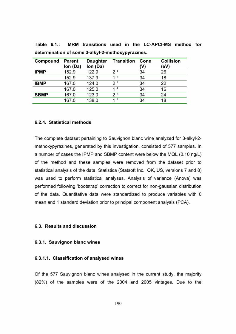
190

Table 6.1.: MRM transitions used in the LC-APCI-MS method for determination of some 3-alkyl-2-methoxypyrazines.


Daughter Ion (Da)

Transition Cone (V)

Collision (eV)

IPMP 152.9 122.9 2 ° 34 26 152.9 137.9 1 ° 34 18 IBMP 167.0 124.0 2 ° 34 22 167.0 125.0 1 ° 34 16 SBMP 167.0 123.0 2 ° 34 24 167.0 138.0 1 ° 34 18

6.2.4. Statistical methods

The complete dataset pertaining to Sauvignon blanc wine analyzed for 3-alkyl-2-

methoxypyrazines, generated by this investigation, consisted of 577 samples. In

a number of cases the IPMP and SBMP content were below the MQL (0.10 ng/L)

of the method and these samples were removed from the dataset prior to

statistical analysis of the data. Statistica (Statsoft Inc., OK, US, versions 7 and 8)

was used to perform statistical analyses. Analysis of variance (Anova) was

performed following ‘bootstrap’ correction to correct for non-gaussian distribution

of the data. Quantitative data were standardized to produce variables with 0

mean and 1 standard deviation prior to principal component analysis (PCA).


6.3.1. Sauvignon blanc wines

6.3.1.1. Classification of analysed wines

Of the 577 Sauvignon blanc wines analysed in the current study, the majority

(82%) of the samples were of the 2004 and 2005 vintages. Due to the

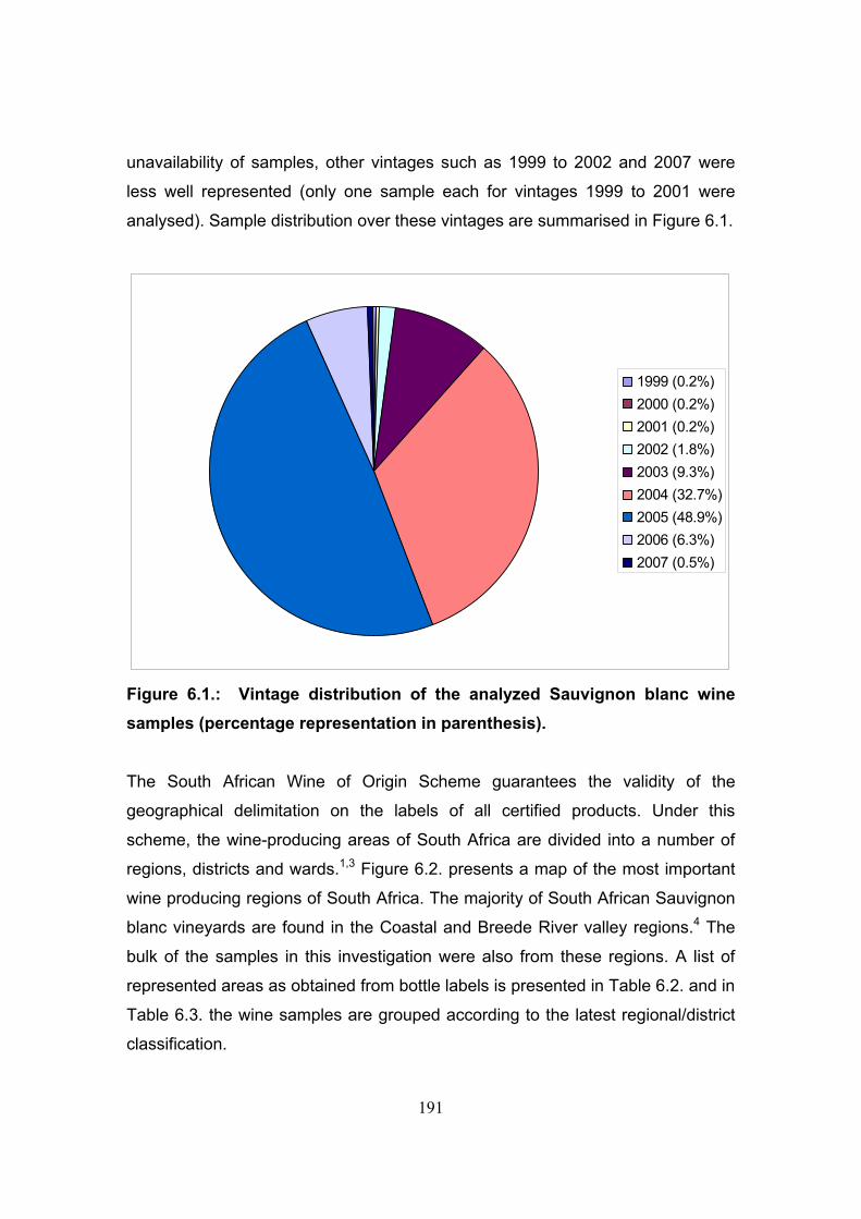
191

unavailability of samples, other vintages such as 1999 to 2002 and 2007 were

less well represented (only one sample each for vintages 1999 to 2001 were

analysed). Sample distribution over these vintages are summarised in Figure 6.1.

1999 (0.2%)2000 (0.2%)2001 (0.2%)2002 (1.8%)2003 (9.3%)2004 (32.7%)2005 (48.9%)2006 (6.3%)2007 (0.5%)

Figure 6.1.: Vintage distribution of the analyzed Sauvignon blanc wine samples (percentage representation in parenthesis).

The South African Wine of Origin Scheme guarantees the validity of the

geographical delimitation on the labels of all certified products. Under this

scheme, the wine-producing areas of South Africa are divided into a number of

regions, districts and wards.1,3 Figure 6.2. presents a map of the most important

wine producing regions of South Africa. The majority of South African Sauvignon

blanc vineyards are found in the Coastal and Breede River valley regions.4 The

bulk of the samples in this investigation were also from these regions. A list of

represented areas as obtained from bottle labels is presented in Table 6.2. and in

Table 6.3. the wine samples are grouped according to the latest regional/district

classification.

192

Figure 6.2.: Wine producing regions of South Africa.

193

Table 6.2.: Distribution of samples over the wine-producing regions of South Africa according to label classification.1

No. Classification on label. No. of samples. 1 Bonnievale 1 2 Bottelary 4 3 Breede River Valley 5 4 Cape Agulhas 5 5 Cape Point 2 6 Cederberg 2 7 Constantia 16 8 Darling 5 9 Devon Valley 1 10 Durbanville 20 11 Elgin 9 12 Elim 7 13 Franschhoek 12 14 Goudini 12 15 Groenekloof 5 16 Klein Rivier 1 17 Coastal Region 65 18 Lutzville 2 19 McGregor 3 20 Nuy 5 21 Paarl 25 22 Prince Albert Valley 1 23 Robertson 54 24 Simonsberg 12 25 Slanghoek 5 26 Stellenbosch 88 27 Swartland 3 28 Tradouw 1 29 Tulbagh 2 30 Walker Bay 9 31 Wellington 8 32 Western Cape** 153 33 Worcester 33 ** = includes all wine producing regions of the Western Cape.

194

Table 6.3.: Distribution of samples according to the latest regional/district classification.3

No. Region/district. No. of samples. 1 Breede River Valley 118 2 - Breedekloof 17 3 - Robertson 58 4 - Worcester 38 5 Coastal Region 268 6 - Cape Point 2 7 - Constantia 16 8 - Darling 10 9 - Paarl 45 10 - Tygerberg 20 11 - Stellenbosch 105 12 - Swartland 3 13 - Tulbagh 2 14 Little Karoo 1 15 - Tradouw 1 16 Olifants River 2 17 - Lutzville Valley 2 19 Cape Agulhas 12 20 Overberg 10 21 Walker Bay 9 22 Cederberg* 2 23 Prince Albert Valley* 1 24 Western Cape** 153 * = wards

** = includes all wine producing regions of the Western Cape.

From the information in Table 6.3. it is evident that of the samples that originated

from a specific area, approximately 91% were from the Breede River Valley and

Coastal regions, where most Sauvignon blanc vineyards are located. Sampling

may therefore be considered as reasonably representative of the overall South

African Sauvignon blanc production as far as geographical origin is concerned.

195

6.3.1.2. Interpretation of quantitative 3-alkyl-2-methoxypyrazine data: Elucidation of criteria for authenticity

Quantitative data for the three major 3-alkyl-2-methoxypyrazines obtained in the

study are presented in Appendix 2 of this thesis. From these data it was

concluded that IBMP is the major 3-alkyl-2-methoxypyrazine in South African

Sauvignon blanc wine. This observation is in agreement with the finding of

various other reports on this subject.5,6,7 It has also been reported that IBMP is

the principal contributor to the vegetal aroma in Sauvignon blanc wine.6 As IBMP

is also the most abundant 3-alkyl-2-methoxypyrazine in green peppers8, it is

apparent that the levels of this compound may be attenuated by the addition of

green pepper extracts to Sauvignon blanc wine.

The concentration of IBMP was therefore identified as a potential parameter that

may be utilized to detect adulteration of South African Sauvignon blanc wine. In

this study, measured values for the IBMP concentration in 575 South African

Sauvignon blanc wines ranged from 0.40 to 44 ng/L with an average of 6.2 ng/L.

Lacey et al. 7 reported values of 0.6 to 38 ng/L in a study of 22 Sauvignon blanc

wines of Australian, New Zealand and French origin. New Zealand Sauvignon

blanc wine contained consistently higher levels of IBMP with an average of 26

ng/L compared to 6.8 ng/L for Australian wines. A study conducted by Allen et

al.6 on eight commercial Sauvignon blanc wines of Australian and New Zealand

origin produced values of 4.7 to 33 ng/L for the IBMP concentration.

It has tentatively been reported that Sauvignon blanc wine as well as some red

wines contain the three major 3-alkyl-2-methoxypyrazines in fairly constant

relative amounts.7,9 Lacey et al. 7 reported that Sauvignon blanc wines in

particular display a ratio of 7:1 (SD = 1.9) for IBMP to IPMP. As IBMP has been

reported to be far more dominant relative to the other 3-alkyl-2-methoxypyrazines

in green peppers (approximately 100:1)8, it follows that adulteration of wine with

this commodity may enrich the levels of IBMP disproportionately. The ratios of

196

relative abundance of the three major 3-alkyl-2-methoxypyrazines may therefore

reveal this form of adulteration. In this study it was determined that the levels of

IPMP varied between < 0.03 and 3.9 ng/L while that of SBMP varied between <

0.03 and 3.2 ng/L. In the study conducted by Lacey et al. 7 concentrations of

IPMP ranging between 0.9 and 5.6 ng/L and of SBMP ranging between 0.1 and

1.3 ng/L were reported. Allen et al. 6 reported IPMP concentrations up to 3.8

ng/L. It should be noted that neither of these authors were able determine IPMP

or SBMP in all the wines that were investigated and that these values therefore

pertain to a subset of the wines in these respective studies.

The improved level of sensitivity (LOQ = 0.10 ng/L) attained with the analytical

method developed in this study facilitates the quantitative determination of three

major 3-alkyl-2-methoxypyrazines in South African Sauvignon blanc wine. The

method is therefore suited to produce data that permits the implementation of

both strategies outlined above.

6.3.1.3. Determination of limits for the occurrence of IBMP in South African Sauvignon blanc wines

The concentrations of IBMP in South African Sauvignon blanc wines are

influenced by a multitude of factors. A close relationship between the climate of

the area and the season and the levels of IBMP in South African Sauvignon

blanc wine has been reported. This grape variety is also sensitive to viticultural

and production factors.5,10,11 This has been attributed to the temperature and light

sensitivity of the 3-alkyl-2-methoxypyrazines.5,10 Significant variance may

therefore be expected for the concentrations of IBMP in South African Sauvignon

blanc wines. Minimum and maximum values found in this investigation were 0.40

and 44 ng/L respectively while the average of all samples was 6.2 ng/L with RSD

of 102% (n = 575). The median was determined to be 4.3 ng/L, indicating that the

197

majority of samples are at the lower end of the scale. The distribution of IBMP

levels in the analyzed wines is presented in Figure 6.3.

020406080

100120140160180

< 13 -

57 -

9

11 - 1

3

15 - 1

7

19 - 2

1

23 - 2

5

27 - 2

9

31 - 3

3

35 - 3

7

39 - 4

1

43 - 4

5

IBMP concentration (ng/L)

Num

ber o

f sam

ples

0

10

20

30

40

50

0 100 200 300 400 500 600

Samples

IBM

P co

ncen

trat

ion

(ng/

L)

020406080

100120140160180

< 13 -

57 -

9

11 - 1

3

15 - 1

7

19 - 2

1

23 - 2

5

27 - 2

9

31 - 3

3

35 - 3

7

39 - 4

1

43 - 4

5

IBMP concentration (ng/L)

Num

ber o

f sam

ples

0

10

20

30

40

50

0 100 200 300 400 500 600

Samples

IBM

P co

ncen

trat

ion

(ng/

L)

Figure 6.3.: Distribution of IBMP levels in 575 analyzed South African Sauvignon blanc wines: Number of samples as a function of concentration (top), and (bottom) concentration of IBMP in each of the samples (Appendix 2).

198

These results show a relatively large variation (RSD = 102%) in the IBMP

concentration across all analyzed wines. It is also evident that the highest

number of samples contains between 1 and 3 ng/L IBMP and that the frequency

decreases from that up to the maximum concentration of 44 ng/L. It is therefore

clear that the regions and vintages should be considered separately in order to

attempt a more accurate classification of the limits for this compound, taking into

consideration the effect of each of these parameters. Table 6.4. presents a

summary of the IBMP content of vintages 2002 to 2006 for wines grouped

according to geographical origin while Table 6.5. presents the same information

for each vintage.

Table 6.4.: IBMP levels and standard deviation (ng/L) in Sauvignon blanc wines from different wine-making regions over vintages 2002-2006 (minimum / maximum / average / number of samples).

Region/district All vintages Standard deviation Breede River Valley 0.66 / 26 / 5.8 / 118 6.0 - Breedekloof 2.6 / 26 / 8.6 / 17 6.8 - Robertson 0.66 / 26 / 5.8 / 58 7.2 - Worcester 1.3 / 17 / 4.6 / 38 3.6 Coastal Region 0.40 / 38 / 6.4 / 267 5.0 - Constantia 6.0 / 20 / 11 / 16 4.2 - Darling 4.6 / 19 / 12 / 10 4.6 - Paarl 0.52 / 24 / 4.0 / 45 5.2 - Tygerberg 0.74 / 38 / 10 / 20 8.0 - Stellenbosch 0.76 / 20 / 5.2 / 105 3.2 Cape Agulhas 4.2 / 42 / 14 / 12 12 Overberg 2.4 / 26 / 9.4 / 10 7.2 Walker Bay 1.2 / 26 / 5.6 / 9 7.6 Western Cape** 0.48 / 44 / 5.4 / 153 7.2 ** = all wine producing areas of the Western Cape.

199

Table 6.5.: IBMP levels (ng/L) in Sauvignon blanc wines from different wine-making regions for the vintages 2002-2006 (minimum / maximum / average / number of samples).

Region/district 2002 2003 2004 2005 2006 Breede River Valley

- Breedekloof 2.6 / 20 / 7.0 / 10 4.4 / 26 / 11 / 7 - Robertson 0.66 / 26 / 6.0 / 51 2.2 / 13 / 5.8 / 4 - Worcester 1.8 / 16 / 6.6 / 3 1.3 / 11 / 3.4 / 17 2.8 / 17 / 5.4 / 18 Coastal Region - Constantia 12 / 18 / 15 / 3 6.6 / 20 / 11 / 12 - Darling 13 / 19 / 15 / 6 - Paarl 0.82 / 7.8 / 3.6 / 16 0.52 / 24 / 4.0 / 26 - Tygerberg 0.74 / 14 / 5.2 / 5 3.6 / 13 / 8.8 / 4 6.4 / 12 / 9.6 / 7 - Stellenbosch 3.4 / 5.6 / 4.4 / 4 0.76 / 20 / 4.8 / 30 1.0 / 16 / 5.4 / 66 2.8 / 10 / 5.4 / 3 Cape Agulhas 4.2 / 14 / 9.6 / 10 Overberg 2.4 / 26 / 8.6 / 4 5.6 / 13 / 9.6 / 4 Walker Bay 1.2 / 8.4 / 3.4 / 7 Western Cape** 1.2 / 7.0 / 3.4 / 4 1.7 / 9.8 / 5.0 / 33 0.48 / 44 / 5.0 / 102 0.58 / 24 / 9.4 / 12 ** = all wine producing areas of the Western Cape.

Maximum values for IBMP show some variance (17 to 44 ng/L) across the wine

producing regions, and over the sampled vintages. The minimum, maximum and

average values obtained for those samples in this investigation for which a specific

regional delimitation were available, are graphically depicted in Figure 6.4. The

maximum value was displayed in black, and at the centre of the three parameters in

this bar graph to clearly illustrate variability across the regions.

0

10

20

30

40

50

Breede

kloof

Robert

son

Worces

ter

Consta

ntia

Darling

Paarl

Tygerb

erg

Stellen

bosc

h

Cape A

gulha

s

Overbe

rg

Walker

Bay

Wester

n Cap

e

IBM

P (n

g/L)

MinMaxAve

Figure 6.4.: Summary of the minimum, maximum and average values of IBMP in Sauvignon blanc wine as a function of region. Only samples with specific regional classification are shown, vintages 1999 to 2007.

From the information in Figure 6.4. it can be observed that some regions such as

Constantia and Darling (cooler climate, close to ocean) are characterized by

relatively high average IBMP values but that their maximum values are nevertheless

lower than those of some warmer (inland) regions like Robertson and Paarl (which

in turn had lower average values). On the other hand, Cape Agulhas, a cool region

in close proximity to the ocean displays a relatively high average and maximum

value. This variable nature of the occurrence of IBMP in South African Sauvignon

blanc wines may be illustrated at the hand of two examples. Figure 6.5. presents an

illustration of the IBMP content of wines produced on the same estate in the

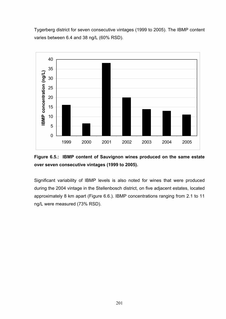
201

Tygerberg district for seven consecutive vintages (1999 to 2005). The IBMP content

varies between 6.4 and 38 ng/L (60% RSD).

0

5

10

15

20

25

30

35

40

1999 2000 2001 2002 2003 2004 2005

IBM

P c

once

ntra

tion

(ng/

L)

Figure 6.5.: IBMP content of Sauvignon wines produced on the same estate over seven consecutive vintages (1999 to 2005).

Significant variability of IBMP levels is also noted for wines that were produced

during the 2004 vintage in the Stellenbosch district, on five adjacent estates, located

approximately 8 km apart (Figure 6.6.). IBMP concentrations ranging from 2.1 to 11

ng/L were measured (73% RSD).

202

0

2

4

6

8

10

12

Estate 1 Estate 2 Estate 3 Estate 4 Estate 5

IBM

P c

once

ntra

tion

(ng/

L)

Figure 6.6.: IBMP content of Sauvignon wines (Stellenbosch, 2004 vintage) produced on five different estates, located in close proximity.

Considering the two illustrations presented above, it is clear that no rigid maximum

values can be set for the concentration of IBMP in South African Sauvignon blanc

wines. The data also suggest that factors such as the region of origin and vintage

are not exclusively determinative regarding the IBMP content of the samples but that

other factors, such as production variables may also play a role in determining the

concentration, an observation supported (to some extent) by some local

research.5,10 The regional data in Table 6.4. seems to reinforce this observation as

there is clearly no obvious correlation between maximum and average values

between the regions, which would indicate that a particular region produces

consistently high values. Cape Agulhas is an exception, producing a high average

and high maximum value. The significance of this is that although a particular region

may posses a low average, a relatively high maximum value may at the same time

be expected, a point that is well illustrated by the data for the Paarl region (Figure

6.4.).

Despite this conclusion, the level of IBMP in wines across all vintages and

geographical origins did not exceed 44 ng/L. Measured values above ~70 ng/L can

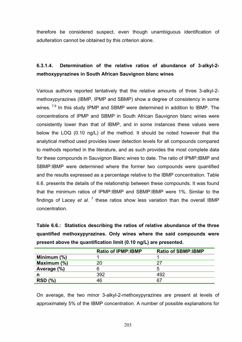
203

therefore be considered suspect, even though unambiguous identification of

adulteration cannot be obtained by this criterion alone.

6.3.1.4. Determination of the relative ratios of abundance of 3-alkyl-2-methoxypyrazines in South African Sauvignon blanc wines

Various authors reported tentatively that the relative amounts of three 3-alkyl-2-

methoxypyrazines (IBMP, IPMP and SBMP) show a degree of consistency in some

wines. 7,9 In this study IPMP and SBMP were determined in addition to IBMP. The

concentrations of IPMP and SBMP in South African Sauvignon blanc wines were

consistently lower than that of IBMP, and in some instances these values were

below the LOQ (0.10 ng/L) of the method. It should be noted however that the

analytical method used provides lower detection levels for all compounds compared

to methods reported in the literature, and as such provides the most complete data

for these compounds in Sauvignon Blanc wines to date. The ratio of IPMP:IBMP and

SBMP:IBMP were determined where the former two compounds were quantified

and the results expressed as a percentage relative to the IBMP concentration. Table

6.6. presents the details of the relationship between these compounds. It was found

that the minimum ratios of IPMP:IBMP and SBMP:IBMP were 1%. Similar to the

findings of Lacey et al. 7 these ratios show less variation than the overall IBMP

concentration.

Table 6.6.: Statistics describing the ratios of relative abundance of the three quantified methoxypyrazines. Only wines where the said compounds were present above the quantification limit (0.10 ng/L) are presented.

Ratio of IPMP:IBMP Ratio of SBMP:IBMP Minimum (%) 1 1 Maximum (%) 20 27 Average (%) 6 5 n 392 492 RSD (%) 46 67

On average, the two minor 3-alkyl-2-methoxypyrazines are present at levels of

approximately 5% of the IBMP concentration. A number of possible explanations for

204

the variation in measured abundances may be found. The fact that South African

producers may (legally)1 add certain undisclosed amounts of wines from other

cultivars to wine labelled as Sauvignon blanc may certainly contribute to the said

variability. The variation of these ratios may also be attributed to different rates of

evolution of the relevant species in the grape prior to harvesting, a phenomenon

reported to occur in Cabernet Sauvignon grapes.12 The time of harvest may then

play a determinative role in the relative abundances.

The relatively large variation in these ratios indicates that no rigid values exist for the

quantitative relationship between the three 3-alkyl-2-methoxypyrazines. A value of

1%, relative to IBMP, may however tentatively be considered as the minimum level

and lower ratios may indicate possible adulteration of the wine sample with a source

rich in IBMP. Such cases may then be evaluated by also taking into consideration

the relative IBMP level of the sample.

Sauvignon blanc leaves were also analyzed in an attempt to determine the ratio

between these components and as the 3-alkyl-2-methoxypyrazines probably

partially originate from the leaves this may possibly provide useful information

pertaining to the relevant abundances.13 Leaves were sampled at two stages of

development, darker green from the top of the vine and smaller light green (young)

leaves from lower down. The samples were collected on the same day in October

during the 2007 season. As the leaves were at a relatively early stage of

development, the concentrations were relatively low with the result that only IBMP

were quantified. The dark green leaves contained 44 ng/kg IBMP and the lighter

leaves 32 ng/kg. Due to time constraints it was not possible to follow the evolution of

the components of interest in the leaves.

6.3.1.5. Determination of the effect of adulteration on the 3-alkyl-2-methoxypyrazine profile

Several green peppers were analyzed as described in the experimental section to

determine the relative amounts of 3-alkyl-2-methoxypyrazines, with the aim of

determining the effect of wine adulteration with pepper extracts. These peppers

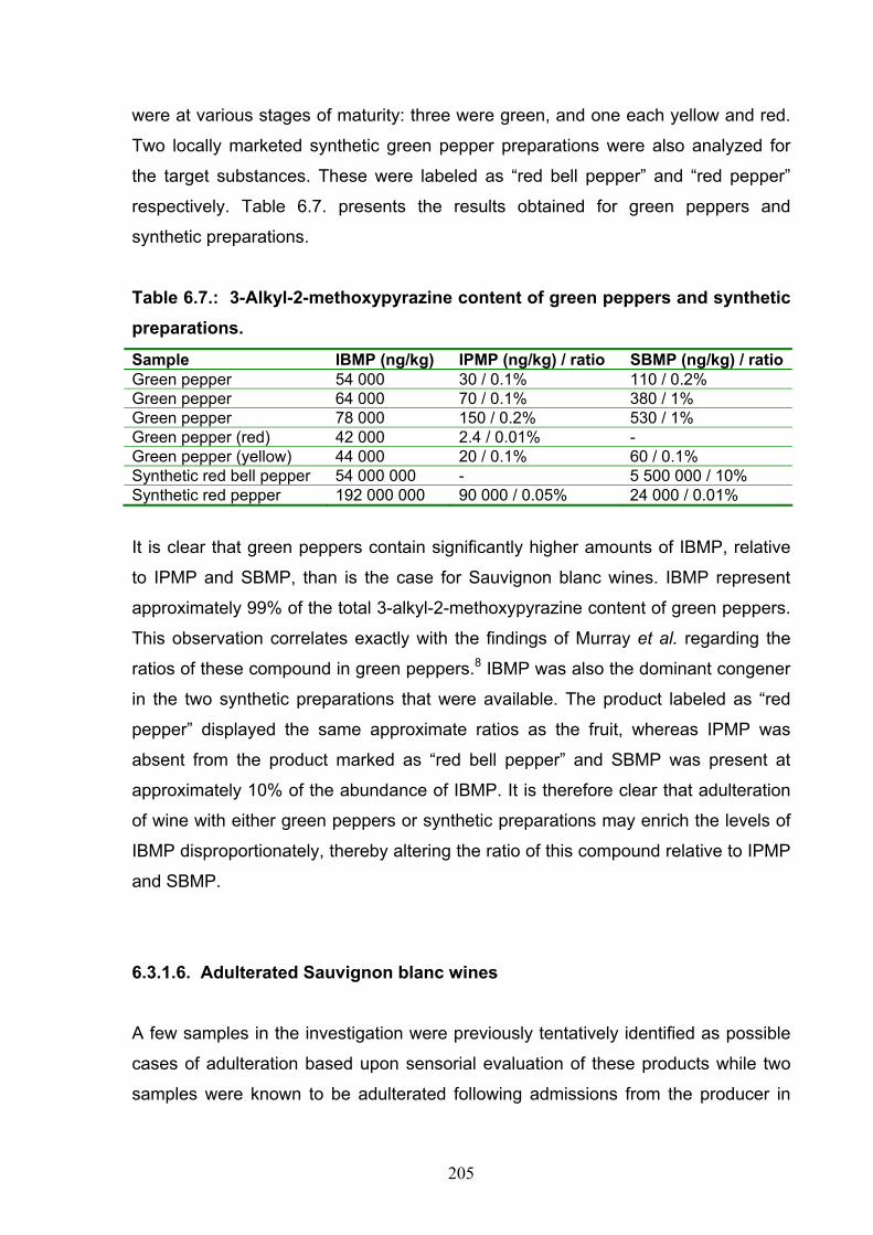
205

were at various stages of maturity: three were green, and one each yellow and red.

Two locally marketed synthetic green pepper preparations were also analyzed for

the target substances. These were labeled as “red bell pepper” and “red pepper”

respectively. Table 6.7. presents the results obtained for green peppers and

synthetic preparations.

Table 6.7.: 3-Alkyl-2-methoxypyrazine content of green peppers and synthetic preparations.

Sample IBMP (ng/kg) IPMP (ng/kg) / ratio SBMP (ng/kg) / ratio Green pepper 54 000 30 / 0.1% 110 / 0.2% Green pepper 64 000 70 / 0.1% 380 / 1% Green pepper 78 000 150 / 0.2% 530 / 1% Green pepper (red) 42 000 2.4 / 0.01% - Green pepper (yellow) 44 000 20 / 0.1% 60 / 0.1% Synthetic red bell pepper 54 000 000 - 5 500 000 / 10% Synthetic red pepper 192 000 000 90 000 / 0.05% 24 000 / 0.01%

It is clear that green peppers contain significantly higher amounts of IBMP, relative

to IPMP and SBMP, than is the case for Sauvignon blanc wines. IBMP represent

approximately 99% of the total 3-alkyl-2-methoxypyrazine content of green peppers.

This observation correlates exactly with the findings of Murray et al. regarding the

ratios of these compound in green peppers.8 IBMP was also the dominant congener

in the two synthetic preparations that were available. The product labeled as “red

pepper” displayed the same approximate ratios as the fruit, whereas IPMP was

absent from the product marked as “red bell pepper” and SBMP was present at

approximately 10% of the abundance of IBMP. It is therefore clear that adulteration

of wine with either green peppers or synthetic preparations may enrich the levels of

IBMP disproportionately, thereby altering the ratio of this compound relative to IPMP

and SBMP.

6.3.1.6. Adulterated Sauvignon blanc wines

A few samples in the investigation were previously tentatively identified as possible

cases of adulteration based upon sensorial evaluation of these products while two

samples were known to be adulterated following admissions from the producer in

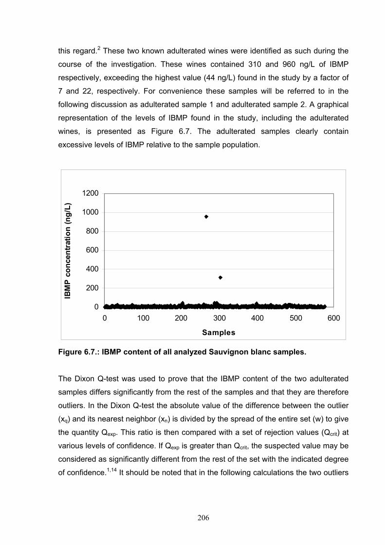
206

this regard.2 These two known adulterated wines were identified as such during the

course of the investigation. These wines contained 310 and 960 ng/L of IBMP

respectively, exceeding the highest value (44 ng/L) found in the study by a factor of

7 and 22, respectively. For convenience these samples will be referred to in the

following discussion as adulterated sample 1 and adulterated sample 2. A graphical

representation of the levels of IBMP found in the study, including the adulterated

wines, is presented as Figure 6.7. The adulterated samples clearly contain

excessive levels of IBMP relative to the sample population.

0

200

400

600

800

1000

1200

0 100 200 300 400 500 600

Samples

IBM

P co

ncen

tratio

n (n

g/L)

Figure 6.7.: IBMP content of all analyzed Sauvignon blanc samples.

The Dixon Q-test was used to prove that the IBMP content of the two adulterated

samples differs significantly from the rest of the samples and that they are therefore

outliers. In the Dixon Q-test the absolute value of the difference between the outlier

(xq) and its nearest neighbor (xn) is divided by the spread of the entire set (w) to give

the quantity Qexp. This ratio is then compared with a set of rejection values (Qcrit) at

various levels of confidence. If Qexp is greater than Qcrit, the suspected value may be

considered as significantly different from the rest of the set with the indicated degree

of confidence.1,14 It should be noted that in the following calculations the two outliers

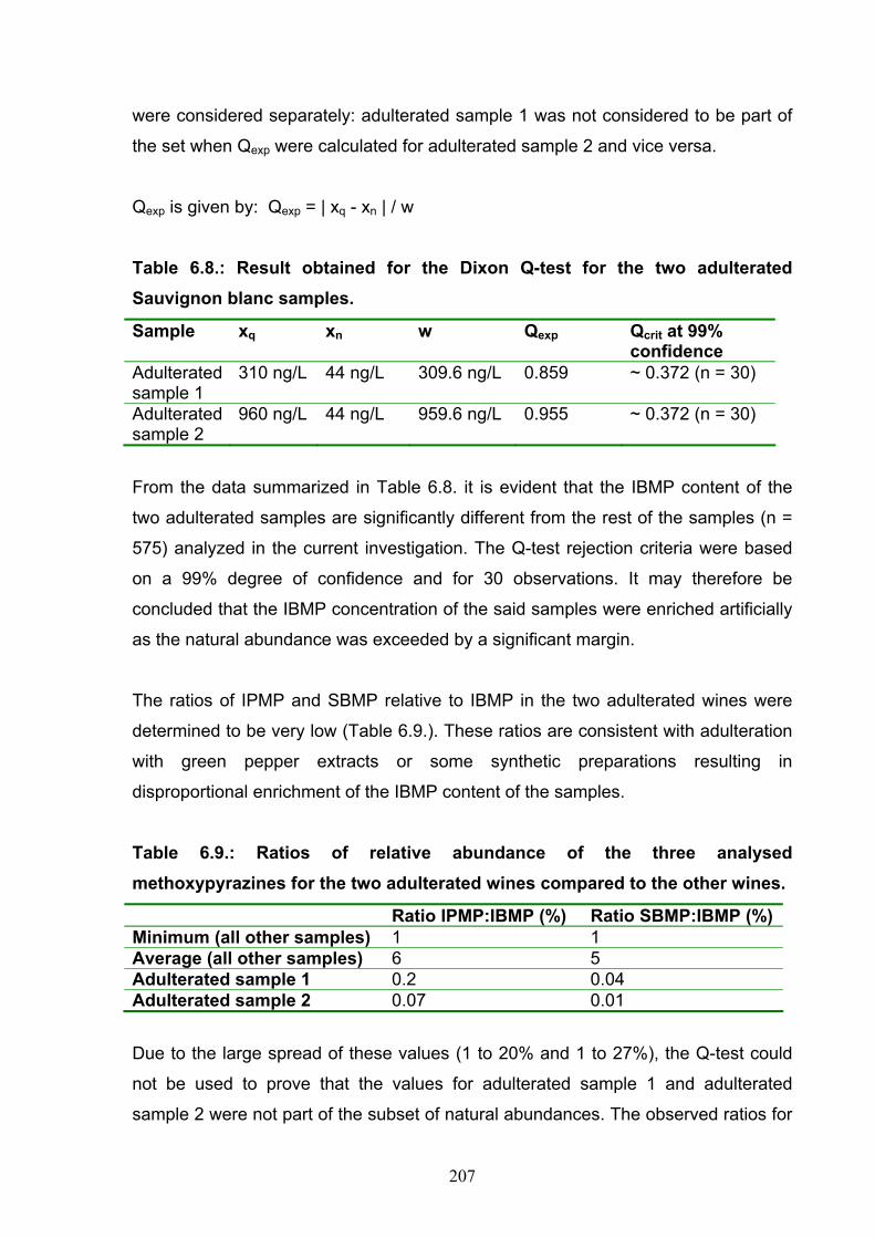
207

were considered separately: adulterated sample 1 was not considered to be part of

the set when Qexp were calculated for adulterated sample 2 and vice versa.

Qexp is given by: Qexp = | xq - xn | / w

Table 6.8.: Result obtained for the Dixon Q-test for the two adulterated Sauvignon blanc samples.

Sample xq xn w Qexp Qcrit at 99% confidence

Adulterated sample 1

310 ng/L 44 ng/L 309.6 ng/L 0.859 ~ 0.372 (n = 30)

Adulterated sample 2

960 ng/L 44 ng/L 959.6 ng/L 0.955 ~ 0.372 (n = 30)

From the data summarized in Table 6.8. it is evident that the IBMP content of the

two adulterated samples are significantly different from the rest of the samples (n =

575) analyzed in the current investigation. The Q-test rejection criteria were based

on a 99% degree of confidence and for 30 observations. It may therefore be

concluded that the IBMP concentration of the said samples were enriched artificially

as the natural abundance was exceeded by a significant margin.

The ratios of IPMP and SBMP relative to IBMP in the two adulterated wines were

determined to be very low (Table 6.9.). These ratios are consistent with adulteration

with green pepper extracts or some synthetic preparations resulting in

disproportional enrichment of the IBMP content of the samples.

Table 6.9.: Ratios of relative abundance of the three analysed methoxypyrazines for the two adulterated wines compared to the other wines.

Ratio IPMP:IBMP (%) Ratio SBMP:IBMP (%) Minimum (all other samples) 1 1 Average (all other samples) 6 5 Adulterated sample 1 0.2 0.04 Adulterated sample 2 0.07 0.01

Due to the large spread of these values (1 to 20% and 1 to 27%), the Q-test could

not be used to prove that the values for adulterated sample 1 and adulterated

sample 2 were not part of the subset of natural abundances. The observed ratios for

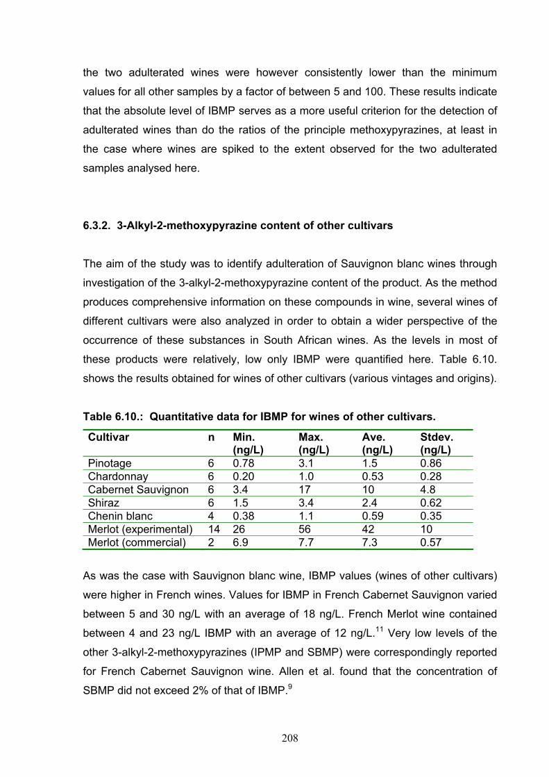
208

the two adulterated wines were however consistently lower than the minimum

values for all other samples by a factor of between 5 and 100. These results indicate

that the absolute level of IBMP serves as a more useful criterion for the detection of

adulterated wines than do the ratios of the principle methoxypyrazines, at least in

the case where wines are spiked to the extent observed for the two adulterated

samples analysed here.

6.3.2. 3-Alkyl-2-methoxypyrazine content of other cultivars

The aim of the study was to identify adulteration of Sauvignon blanc wines through

investigation of the 3-alkyl-2-methoxypyrazine content of the product. As the method

produces comprehensive information on these compounds in wine, several wines of

different cultivars were also analyzed in order to obtain a wider perspective of the

occurrence of these substances in South African wines. As the levels in most of

these products were relatively, low only IBMP were quantified here. Table 6.10.

shows the results obtained for wines of other cultivars (various vintages and origins).

Table 6.10.: Quantitative data for IBMP for wines of other cultivars.

Cultivar n Min. (ng/L)

Max. (ng/L)

Ave. (ng/L)

Stdev. (ng/L)

Pinotage 6 0.78 3.1 1.5 0.86 Chardonnay 6 0.20 1.0 0.53 0.28 Cabernet Sauvignon 6 3.4 17 10 4.8 Shiraz 6 1.5 3.4 2.4 0.62 Chenin blanc 4 0.38 1.1 0.59 0.35 Merlot (experimental) 14 26 56 42 10 Merlot (commercial) 2 6.9 7.7 7.3 0.57

As was the case with Sauvignon blanc wine, IBMP values (wines of other cultivars)

were higher in French wines. Values for IBMP in French Cabernet Sauvignon varied

between 5 and 30 ng/L with an average of 18 ng/L. French Merlot wine contained

between 4 and 23 ng/L IBMP with an average of 12 ng/L.11 Very low levels of the

other 3-alkyl-2-methoxypyrazines (IPMP and SBMP) were correspondingly reported

for French Cabernet Sauvignon wine. Allen et al. found that the concentration of

SBMP did not exceed 2% of that of IBMP.9

209

No information was obtained for other cultivars in Table 6.10. Pinotage is a cultivar

that is unique to South Africa and to the best of our knowledge these compounds

have never been detected in these wines. The experimental Merlot samples

produced very high levels relative to the other South African wines. The

experimental Merlot wines were produced from a single experimental vineyard

where the effect of different viticultural practices was studied. Although a detailed

evaluation of these parameters on the IBMP content of the wines falls outside the

scope of the current work, it can be noted that differences in viticultural practices

have a significant effect on the IBMP content (a factor two for the same vintage,

vineyard and clone in this example).

6.3.3. Multivariate analysis of the 3-alkyl-2-methoxypyrazine data

A number of multivariate data analysis techniques exists that may be utilized to

extract useful information from complex data sets. The key to obtain the desired

information is to establish the objective of the investigation clearly. Multivariate data

analysis (MVA) may be used to achieve three main aims, namely: data description,

discrimination and classification, and regression and prediction.15 In this study

principal component analysis (PCA) was utilized to study the differences between

wine samples (discrimination) in the methoxypyrazine dataset. The objectives of the

PCA study were to confirm the conclusions regarding the adulterated wines as well

as to study possible correlations between the data and vintage and region of origin

of the products. The latter was attempted because for such a large dataset

containing many variables, it is not easy to visualize such correlations.

6.3.3.1. Brief overview of PCA

PCA involves transformation of a set of correlated variables to a set of uncorrelated

factors (referred to as principal components or PC’s) in such a manner that the

underlying covariance is maximized.15 The utility of PCA stems from the fact that the

derived variables are often better descriptors of the data structure than the original

210

variables. As a large part of the variance in the original dataset can be modeled by a

limited number of latent variables, PCA effectively reduces the dimensionality of the

data and in this way facilitates visual inspection of complex data sets.15,16 The

results of PCA are therefore commonly interpreted visually. As the total variance

within the data set is mainly accounted for by the first few PC’s, these may be used

plot the data. The similarity or differences between objects (samples) may then be

determined readily from these plots.

The original variables are related to the PC’s, and loading vectors, also called

loadings, may be viewed as the bridge between these entities. Loadings reveal the

extent of the contribution of each variable to meaningful variation in the data.15

Therefore the loadings of each of the original variables plotted against the derived

latent variables produces a loadings plot that may be used to identify those variables

responsible for differentiation of samples on each PC. From the loadings plot the

correlation (i.e. co-variance) between variables may also be determined, with the

angle between loading vectors indicative of their correlation. This is used to study

potential relationships between the original variables. On the other hand, a scores

plot depicts the scores of each object or sample on selected PCs, and is used to

study the relationships between samples. Distinct clusters would reveal the grouping

of similar objects. Typically, scores plots are used to investigate potential grouping

of samples, while subsequent investigation of loadings plots can be used to

determine which variables are responsible for this differentiation between samples.

6.3.3.2. Results for adulterated wines

PCA was first applied in order to corroborate results for outliers (adulterated

samples 1 and 2, numbered 18 and 19) with those obtained by univariate statistics.

To investigate the two outliers PCA was performed using only IPMP, IBMP and

SBMP variables. The loading plot for PC1 and PC2 (Figure 6.8.) reveals that IPMP

and SBMP are positively correlated with PC1 while IBMP is likewise correlated with

PC2. The loading vector for IBMP is approximately orthogonal to those of IPMP and

SBMP, indicating that these variables do not covary. The IBMP content therefore

plays a minor role in discriminating wines according to PC1 and vice versa. The

211

score plot clearly show the two adulterated samples differentiated on PC2. These

two samples are therefore distinguished based on their (high) IBMP content. Sample

96 is distinguished on PC1, based on a high IPMP and SBMP content. This product

is a barrel-fermented Sauvignon blanc wine, indicating that this wine style may

possibly be correlated with high ratios (IPMP:IBMP and SBMP:IBMP) as values of

13 and 16% were obtained, compared to mean values of ~5%. Regarding the

following figures, it should be noted that the term “factor” (Statistica) refers to the

principal component (PC).

Projection of the variables on the factor-plane ( 1 x 2)

Active

IBMP (ng/L)

SBMP (ng/L

IPMP (ng/L

-1.0 -0.5 0.0 0.5 1.0

Factor 1 : 57.27%

-1.0

-0.5

0.0

0.5

1.0

Fact

or 2

: 32

.81%

IBMP (ng/L)

SBMP (ng/L)

IPMP (ng/L)

Projection of the cases on the factor-plane ( 1 x 2)Cases with sum of cosine square >= 0.00

Active

446211811914264 145141 42115111131 73125 76122 123360442452581426431 583425171578 262319400544528 226524 26331 20247414479511219562165449461595

96506

241273 410204 16260482446263274168 296459258297 238517202413306501 526167282084804301321401403 1029825551903773993332437466290291586373 46528143555041820650459620015222 4121645722054234543742075022795634 935410387138523839468410831731847113823135190316 100105109 999145 31436104106308865789312 355383 1103093159298143310311140 107101 88493 261406 328558600711333243 18521430323323239283250 481350253254553248383299516 539588276552577 40529 25139633040219751421527 18354754556534556455917 433201460 540153576293505441156326523 487 211543566162193 371343580432434212 574157277416489521348453507 6470152209415478 411522451 198176475598158510 554508579448199444531352594494407292 5353035426531169 601602 603604155196468483 605490417252172355149571150179 430560228218282335 467181584215294

58 6341 65404811713969685961671341354911466137116 80129130126781287772 12470747113213375 11281 127

18

19

-4 -2 0 2 4 6 8 10 12

Factor 1: 57.27%

-5

0

5

10

15

Fact

or 2

: 32.

81%

446211811914264 145141 42115111131 73125 76122 123360442452581426431 583425171578 262319400544528 226524 26331 20247414479511219562165449461595

96506

241273 410204 16260482446263274168 296459258297 238517202413306501 526167282084804301321401403 1029825551903773993332437466290291586373 46528143555041820650459620015222 4121645722054234543742075022795634 935410387138523839468410831731847113823135190316 100105109 999145 31436104106308865789312 355383 1103093159298143310311140 107101 88493 261406 328558600711333243 18521430323323239283250 481350253254553248383299516 539588276552577 40529 25139633040219751421527 18354754556534556455917 433201460 540153576293505441156326523 487 211543566162193 371343580432434212 574157277416489521348453507 6470152209415478 411522451 198176475598158510 554508579448199444531352594494407292 5353035426531169 601602 603604155196468483 605490417252172355149571150179 430560228218282335 467181584215294

58 6341 65404811713969685961671341354911466137116 80129130126781287772 12470747113213375 11281 127

18

19


Active

IBMP (ng/L)

SBMP (ng/L

IPMP (ng/L

-1.0 -0.5 0.0 0.5 1.0

Factor 1 : 57.27%

-1.0

-0.5

0.0

0.5

1.0

Fact

or 2

: 32

.81%

IBMP (ng/L)

SBMP (ng/L)

IPMP (ng/L)


Active

446211811914264 145141 42115111131 73125 76122 123360442452581426431 583425171578 262319400544528 226524 26331 20247414479511219562165449461595

96506

241273 410204 16260482446263274168 296459258297 238517202413306501 526167282084804301321401403 1029825551903773993332437466290291586373 46528143555041820650459620015222 4121645722054234543742075022795634 935410387138523839468410831731847113823135190316 100105109 999145 31436104106308865789312 355383 1103093159298143310311140 107101 88493 261406 328558600711333243 18521430323323239283250 481350253254553248383299516 539588276552577 40529 25139633040219751421527 18354754556534556455917 433201460 540153576293505441156326523 487 211543566162193 371343580432434212 574157277416489521348453507 6470152209415478 411522451 198176475598158510 554508579448199444531352594494407292 5353035426531169 601602 603604155196468483 605490417252172355149571150179 430560228218282335 467181584215294

58 6341 65404811713969685961671341354911466137116 80129130126781287772 12470747113213375 11281 127

18

19

-4 -2 0 2 4 6 8 10 12

Factor 1: 57.27%

-5

0

5

10

15

Fact

or 2

: 32.

81%

446211811914264 145141 42115111131 73125 76122 123360442452581426431 583425171578 262319400544528 226524 26331 20247414479511219562165449461595

96506

241273 410204 16260482446263274168 296459258297 238517202413306501 526167282084804301321401403 1029825551903773993332437466290291586373 46528143555041820650459620015222 4121645722054234543742075022795634 935410387138523839468410831731847113823135190316 100105109 999145 31436104106308865789312 355383 1103093159298143310311140 107101 88493 261406 328558600711333243 18521430323323239283250 481350253254553248383299516 539588276552577 40529 25139633040219751421527 18354754556534556455917 433201460 540153576293505441156326523 487 211543566162193 371343580432434212 574157277416489521348453507 6470152209415478 411522451 198176475598158510 554508579448199444531352594494407292 5353035426531169 601602 603604155196468483 605490417252172355149571150179 430560228218282335 467181584215294

58 6341 65404811713969685961671341354911466137116 80129130126781287772 12470747113213375 11281 127

18

19

Figure 6.8.: PCA analysis to discriminate adulterated samples, only IPMP, IBMP and SBMP variables.

6.3.3.3. Grouping of wine samples according to geographical origin

It has been hypothesized that region of origin plays an important role in determining

the 3-alkyl-2-methoxypyrazine content of Sauvignon blanc wines. Quantitative

differences were reported between French, New Zealand and Australian products6,7

as well as between locally produced wines, with different origins5,10. Local

investigations attributed regional differences in IBMP concentration to macro- and

microclimatic variations between regions and seasons.10 PCA and Anova were used

to investigate possible grouping of samples according to origin.

212

Grouping of wine samples according to origin and the possible existence of a

relationship between 3-alkyl-2-methoxypyrazine content and other wine parameters

(alcohol and reducing sugar content, total acidity and pH) were investigated using

PCA with the objective to use this information for authenticity elucidation. The two

outliers (adulterated sample 1 and 2) and samples with non-specific regional

classification (such as Western Cape), were removed from the dataset. Firstly all

variables were used (IPMP, IBMP and SBMP concentration as well as alcohol and

reducing sugar content, pH and total acidity) and then secondly only the

methoxypyrazine variables. The loading plot shows that in PC2 total acidity (TA) and

pH are inversely related (as expected, high acidity leads to low wine pH). PC1

accounts for 35% of the variance, and the methoxypyrazines are responsible for

variation explained by this PC. Significant correlation (covariance) between the three

methoxypyrazines are observed on PC1 (Figure 6.9.).

Figure 6.9.: PCA analysis for grouping of samples according to region of origin, all variables included (PC1 versus PC2).

No clear distinction according to region is evident from the score plot although some

samples are differentiated based on high methoxypyrazine content and are

positioned to the left in Figure 6.9. PC1 versus PC3 distinguishes a single wine from

Constantia but this separation is based on an unusually high sugar content for this

noble late harvest wine (Figure 6.10.). Omission of this sweet Constantia wine from

the relevant dataset yielded no significant improvement in the separation (not

shown).


Active

IBMP (ng/L)

SBMP (ng/L)

IPMP (ng/L)

Alc (% v/v)

Sug (g/L)

pH

T.A. (g/L)

-1.0 -0.5 0.0 0.5 1.0

Factor 1 : 35.46%

-1.0

-0.5

0.0

0.5

1.0

Fact

or 2

: 18

.27%

IBMP (ng/L)

SBMP (ng/L)

IPMP (ng/L)

Alc (% v/v)

Sug (g/L)

pH

T.A. (g/L)


Active-12 -10 -8 -6 -4 -2 0 2 4

Factor 1: 35.46%

-5

-4

-3

-2

-1

0

1

2

3

4

5

Fact

or 2

: 18.

27%

213

Figure 6.10.: PCA analysis for grouping of samples according to region of origin with all variables included, PC1 versus PC3.

The same analysis was then performed but using only three variables (IPMP, IBMP

and SBMP). Here PC1 accounts for variation in overall methoxypyrazine content

while in PC2 IBMP and IPMP are inversely correlated to SBMP (Figure 6.11.).

Figure 6.11.: PCA analysis for grouping of samples according to region of origin, only IPMP, IBMP and SBMP variables, PC1 versus PC2.


Active-12 -10 -8 -6 -4 -2 0 2 4

Factor 1: 35.46%

0

5

10

15

Fact

or 3

: 16.

20%


Active

IBMP (ng/L)

SBMP (ng/L)

IPMP (ng/L)

-1.0 -0.5 0.0 0.5 1.0

Factor 1 : 81.09%

-1.0

-0.5

0.0

0.5

1.0

Fact

or 2

: 14

.94%

IBMP (ng/L)

SBMP (ng/L)

IPMP (ng/L)


Active

BreedekloofBreedekloofBreedekloofBreedekloof

BreedekloofBreedekloof



BreedekloofBreedekloofBreedekloofBreedekloofBreedekloofBreedekloof

Breedekloof

Cape AgulhasCape AgulhasCape AgulhasCape Agulhas


Cape AgulhasCape Agulhas

Cape Agulhas

Cape Agulhas

Cape Point

Cape PointCederberg

Cederberg

ConstantiaConstantiaConstantiaConstantia

ConstantiaConstantia


Constantia

Constantia


Constantia

Constantia

DarlingDarlingDarling


DarlingDarling DarlingDarlingLutzville

Lutzville

OverbergOverbergOverberg

Overberg Overberg

OverbergOverbergOverbergOverberg

Overberg

Paarl

PaarlPaarlPaarl

PaarlPaarlPaarl

PaarlPaarlPaarl

PaarlPaarlPaarlPaarlPaarlPaarl Paarl

PaarlPaarlPaarl

Paarl

Paarl Paarl

PaarlPaarl

PaarlPaarlPaarl

PaarlPaarlPaarlPaarlPaarlPaarl

Paarl

Paarl

PaarlPaarl

PaarlPaarlPaarlPaarl

PaarlPaarl

PaarlRobertsonRobertson

RobertsonRobertsonRobertson

RobertsonRobertsonRobertsonRobertsonRobertsonRobertsonRobertson

RobertsonRobertsonRobertsonRobertsonRobertsonRobertsonRobertsonRobertsonRobertsonRobertson



RobertsonRobertsonRobertsonRobertsonRobertson

RobertsonRobertsonRobertsonRobertson


RobertsonRobertson

RobertsonRobertsonRobertsonRobertsonRobertsonRobertsonRobertson Robertson

RobertsonRobertson


Robertson

RobertsonStellenboschStellenbosch

Stellenbosch

StellenboschStellenboschStellenboschStellenboschStellenboschStellenbosch

StellenboschStellenboschStellenboschStellenbosch StellenboschStellenboschStellenbosch

StellenboschStellenbosch

StellenboschStellenboschStellenboschStellenbosch

Stellenbosch

StellenboschStellenboschStellenbosch

Stellenbosch StellenboschStellenboschStellenboschStellenboschStellenboschStellenboschStellenboschStellenboschStellenboschStellenbosch

StellenboschStellenboschStellenboschStellenboschStellenbosch



Stellenbosch


Stellenbosch


StellenboschStellenboschStellenbosch Stellenbosch











Stellenbosch



Swartland

SwartlandSwartlandTulbaghTulbagh

TygerbergTygerberg

Tygerberg

Tygerberg

TygerbergTygerbergTygerberg

Tygerberg

Tygerberg

TygerbergTygerberg

Tygerberg

TygerbergTygerberg

Tygerberg

TygerbergTygerbergTygerbergTygerberg

Tygerberg

Walker BayWalker BayWalker BayWalker BayWalker Bay

Walker BayWalker BayWalker Bay

Walker Bay

WorcesterWorcesterWorcesterWorcesterWorcesterWorcesterWorcesterWorcesterWorcesterWorcester

WorcesterWorcesterWorcesterWorcesterWorcester

WorcesterWorcester

WorcesterWorcester

Worcester

WorcesterWorcesterWorcesterWorcesterWorcesterWorcesterWorcesterWorcester

WorcesterWorcesterWorcesterWorcesterWorcesterWorcester

WorcesterWorcesterWorcesterWorcester

-12 -10 -8 -6 -4 -2 0 2 4

Factor 1: 81.09%

-8

-6

-4

-2

0

2

4

Fact

or 2

: 14.

94%

BreedekloofBreedekloofBreedekloofBreedekloof




BreedekloofBreedekloofBreedekloofBreedekloofBreedekloofBreedekloof

Breedekloof



Cape AgulhasCape Agulhas

Cape Agulhas

Cape Agulhas

Cape Point

Cape PointCederberg

Cederberg




Constantia

Constantia


Constantia

Constantia



DarlingDarling DarlingDarlingLutzville

Lutzville

OverbergOverbergOverberg

Overberg Overberg

OverbergOverbergOverbergOverberg

Overberg

Paarl

PaarlPaarlPaarl

PaarlPaarlPaarl

PaarlPaarlPaarl

PaarlPaarlPaarlPaarlPaarlPaarl Paarl

PaarlPaarlPaarl

Paarl

Paarl Paarl

PaarlPaarl

PaarlPaarlPaarl

PaarlPaarlPaarlPaarlPaarlPaarl

Paarl

Paarl

PaarlPaarl

PaarlPaarlPaarlPaarl

PaarlPaarl

PaarlRobertsonRobertson


RobertsonRobertsonRobertsonRobertsonRobertsonRobertsonRobertson

RobertsonRobertsonRobertsonRobertsonRobertsonRobertsonRobertsonRobertsonRobertsonRobertson



RobertsonRobertsonRobertsonRobertsonRobertson



RobertsonRobertson

RobertsonRobertsonRobertsonRobertsonRobertsonRobertsonRobertson Robertson

RobertsonRobertson


Robertson

RobertsonStellenboschStellenbosch

Stellenbosch


StellenboschStellenboschStellenboschStellenbosch StellenboschStellenboschStellenbosch



Stellenbosch


Stellenbosch StellenboschStellenboschStellenboschStellenboschStellenboschStellenboschStellenboschStellenboschStellenboschStellenbosch




Stellenbosch


Stellenbosch


StellenboschStellenboschStellenbosch Stellenbosch











Stellenbosch



Swartland

SwartlandSwartlandTulbaghTulbagh

TygerbergTygerberg

Tygerberg

Tygerberg

TygerbergTygerbergTygerberg

Tygerberg

Tygerberg

TygerbergTygerberg

Tygerberg

TygerbergTygerberg

Tygerberg

TygerbergTygerbergTygerbergTygerberg

Tygerberg

Walker BayWalker BayWalker BayWalker BayWalker Bay

Walker BayWalker BayWalker Bay

Walker Bay

WorcesterWorcesterWorcesterWorcesterWorcesterWorcesterWorcesterWorcesterWorcesterWorcester

WorcesterWorcesterWorcesterWorcesterWorcester

WorcesterWorcester

WorcesterWorcester

Worcester

WorcesterWorcesterWorcesterWorcesterWorcesterWorcesterWorcesterWorcester

WorcesterWorcesterWorcesterWorcesterWorcesterWorcester

WorcesterWorcesterWorcesterWorcester

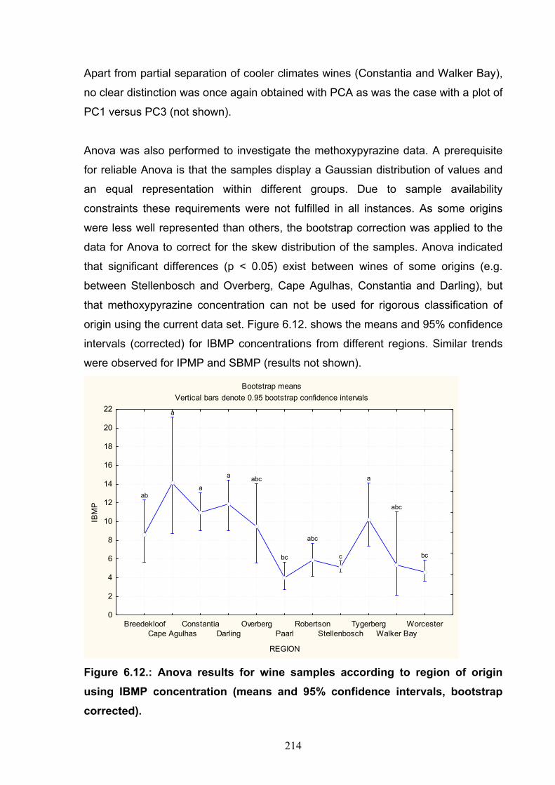
214

Apart from partial separation of cooler climates wines (Constantia and Walker Bay),

no clear distinction was once again obtained with PCA as was the case with a plot of

PC1 versus PC3 (not shown).

Anova was also performed to investigate the methoxypyrazine data. A prerequisite

for reliable Anova is that the samples display a Gaussian distribution of values and

an equal representation within different groups. Due to sample availability

constraints these requirements were not fulfilled in all instances. As some origins

were less well represented than others, the bootstrap correction was applied to the

data for Anova to correct for the skew distribution of the samples. Anova indicated

that significant differences (p < 0.05) exist between wines of some origins (e.g.

between Stellenbosch and Overberg, Cape Agulhas, Constantia and Darling), but

that methoxypyrazine concentration can not be used for rigorous classification of

origin using the current data set. Figure 6.12. shows the means and 95% confidence

intervals (corrected) for IBMP concentrations from different regions. Similar trends

were observed for IPMP and SBMP (results not shown).

Figure 6.12.: Anova results for wine samples according to region of origin using IBMP concentration (means and 95% confidence intervals, bootstrap corrected).

Bootstrap meansVertical bars denote 0.95 bootstrap confidence intervals

BreedekloofCape Agulhas

ConstantiaDarling

OverbergPaarl

RobertsonStellenbosch

TygerbergWalker Bay

Worcester

REGION

0

2

4

6

8

10

12

14

16

18

20

22

IBM

P

ab

a

a

a abc

bc

abc

c

a

abc

bc

215

For the following figures only two distinct regions were compared (Constantia (C)

and Worcester (Wo)), as these regions are relatively cool and warm respectively

and more pronounced differences are therefore expected.

The loading plot for all variables reveals that the pyrazines contribute almost

exclusively to PC1 while the other variables contribute mainly to PC2 (Figure 6.13.).

TA and pH are also directly related here as opposed to before (with all regions). The

spreading of Constantia (C) wines to the right on the score plot are due to higher

methoxypyrazine values while the one sample distinguished on PC2 is due to the

high sugar content of that sample (noble late harvest wine). When the analyses was

performed on the same subset, but with the two extreme C-values omitted, a slight

but inconclusive improvement was observed (results not shown).


Active

IBMP-N(%)SBMP-N(%IPMP-N(%

Alc (% v/v)

Sug (g/L)

pH

T.A. (g/L)

-1.0 -0.5 0.0 0.5 1.0

Factor 1 : 39.74%

-1.0

-0.5

0.0

0.5

1.0

Fact

or 2

: 22

.81%


Active

C

CCC

C CC

CCC

C

C

C

CCWO

WOWOWOWO WOWO

WOWO

WO WO

WO

WOWO

WO

WOWO

WOWO

WOWO

WOWO

WO

WO

-2 0 2 4 6

Factor 1: 39.74%

-2

0

2

4

6

8

Fact

or 2

: 22.

81%


Active

IBMP-N(%)SBMP-N(%IPMP-N(%

Alc (% v/v)

Sug (g/L)

pH

T.A. (g/L)

-1.0 -0.5 0.0 0.5 1.0

Factor 1 : 39.74%

-1.0

-0.5

0.0

0.5

1.0

Fact

or 2

: 22

.81%


Active

C

CCC

C CC

CCC

C

C

C

CCWO

WOWOWOWO WOWO

WOWO

WO WO

WO

WOWO

WO

WOWO

WOWO

WOWO

WOWO

WO

WO

-2 0 2 4 6

Factor 1: 39.74%

-2

0

2

4

6

8

Fact

or 2

: 22.

81%

Figure 6.13.: PCA analysis for grouping of samples according to region of origin (only wines from Constantia (C) and Worcester (Wo) included), using all variables, PC1 versus PC2.

Similar differentiation is observed on the score plot of PC1 versus PC3, mainly due

to differences in methoxypyrazines content (Figure 6.14.). Although no clear

separation was achieved, it can however be accepted that Constantia (C) produces

Sauvignon blanc wine with slightly higher methoxypyrazine concentrations.

216


Active

C

C C

C

C

CC

CC

CCC

C

C

C

WO

WO

WO

WO

WO

WO

WO

WO

WO

WO WO

WO

WO

WO

WOWO

WO

WO

WOWO

WOWO

WO

WO

WO

-2 0 2 4 6

Factor 1: 39.74%

-2

-1

0

1

2

Fact

or 3

: 15.

40%

Figure 6.14.: PCA analysis for grouping of samples according to region of origin for samples from Constantia (C) and Worcester (Wo), using all variables, PC1 versus PC3.

The same subset of samples was analyzed using only the three methoxypyrazine

values for each sample. The loading plot now shows that the three variables are

mainly correlated (negatively) with PC1 while the score plot displays slight

differentiation of some Constantia wines, attributed mainly to this PC. Once again

some differentiation is possible without complete separation (Figure 6.15.). PC1

versus PC3 produced similar results (not shown).

217


Active

IBMP-N(%)

SBMP-N(%)

PMP-N(%)

-1.0 -0.5 0.0 0.5 1.0

Factor 1 : 85.59%

-1.0

-0.5

0.0

0.5

1.0Fa

ctor

2 :

12.1

5%


Active

C

C

C

CC

CC

C

CC

CCC

C

C

WO

WO

WOWO

WOWOWOWOWO

WO

WO

WO

WOWOWO

WOWOWO

WO

WO WO

WO

WOWO

WO

-8 -6 -4 -2 0 2

Factor 1: 85.59%

-1.0

-0.5

0.0

0.5

1.0

1.5

2.0

Fact

or 2

: 12.

15%


Active

IBMP-N(%)

SBMP-N(%)

PMP-N(%)

-1.0 -0.5 0.0 0.5 1.0

Factor 1 : 85.59%

-1.0

-0.5

0.0

0.5

1.0Fa

ctor

2 :

12.1

5%


Active

C

C

C

CC

CC

C

CC

CCC

C

C

WO

WO

WOWO

WOWOWOWOWO

WO

WO

WO

WOWOWO

WOWOWO

WO

WO WO

WO

WOWO

WO

-8 -6 -4 -2 0 2

Factor 1: 85.59%

-1.0

-0.5

0.0

0.5

1.0

1.5

2.0

Fact

or 2

: 12.

15%

Figure 6.15.: PCA analysis for grouping of samples according to region of origin for samples from Constantia (C) and Worcester (Wo), using methoxypyrazine variables, PC1 versus PC2.

Anova revealed that significant differences exist between wines from Constantia and

Worcester (p < 0.05). It should be noted though that the limiting factors discussed

for Anova is also valid here due to sample availability constraints.

As these PCA results did not show clear separation of these two regions (Constantia

and Worcester), the exercise was repeated using data for Stellenbosch (ST) and

Paarl (P). The loading plot for all variables revealed the same trends as discussed

before for Constantia and Worcester. The methoxypyrazines carry approximately

the same weight in PC1 but almost none in PC2. No improved separation was

obtained for these samples compared with the previous combination.

The loading plot of PC1 versus PC2 utilizing only the methoxypyrazine data

revealed that the three pyrazines are negatively correlated (to the same extent) on

PC1, while their loadings on PC2 were smaller (IBMP was positively, and IPMP and

SBMP negatively correlated on this PC). A slightly improved separation was

obtained with Paarl (P) confined mostly to positive PC1 and 2, possibly due to lower

total methoxypyrazines with relatively higher IBMP. PC1 versus PC3 produced no

additional information (Figure 6.16.).

218


Active

P

P

P

PP

P

P

P

P

P

P

P

PP

P

ST

ST

ST

ST

ST STST

ST

ST

ST

ST

ST

ST

STSTST

ST

ST

ST

ST

STST

ST

ST ST

ST

ST

ST

STST

ST

ST

ST ST

ST

ST

ST

ST ST

ST

ST

ST

ST

ST ST

ST

ST

ST

ST

ST

STST

ST

ST

STSTST

ST

ST

-5 -4 -3 -2 -1 0 1 2

Factor 1: 30.95%

-3

-2

-1

0

1

2

3

4Fa

ctor

2: 2

5.00

%


Active

P

P

P

P

P

PP

PP

P

PP

P

P

P

ST

ST STSTST

ST

ST

ST

ST

STST

ST

ST

ST

ST

ST

ST

ST

ST

ST STST

STST STST

ST

ST

STSTSTSTST

ST

ST

ST ST

ST

ST STSTST

ST

ST

STST

STSTST

ST

ST

STST

ST

ST

ST

ST

ST

ST

-5 -4 -3 -2 -1 0 1 2

Factor 1: 71.72%

-2

-1

0

1

2

3

Fact

or 2

: 16.

89%


Active

P

P

P

PP

P

P

P

P

P

P

P

PP

P

ST

ST

ST

ST

ST STST

ST

ST

ST

ST

ST

ST

STSTST

ST

ST

ST

ST

STST

ST

ST ST

ST

ST

ST

STST

ST

ST

ST ST

ST

ST

ST

ST ST

ST

ST

ST

ST

ST ST

ST

ST

ST

ST

ST

STST

ST

ST

STSTST

ST

ST

-5 -4 -3 -2 -1 0 1 2

Factor 1: 30.95%

-3

-2

-1

0

1

2

3

4Fa

ctor

2: 2

5.00

%


Active

P

P

P

P

P

PP

PP

P

PP

P

P

P

ST

ST STSTST

ST

ST

ST

ST

STST

ST

ST

ST

ST

ST

ST

ST

ST

ST STST

STST STST

ST

ST

STSTSTSTST

ST

ST

ST ST

ST

ST STSTST

ST

ST

STST

STSTST

ST

ST

STST

ST

ST

ST

ST

ST

ST

-5 -4 -3 -2 -1 0 1 2

Factor 1: 71.72%

-2

-1

0

1

2

3

Fact

or 2

: 16.

89%

Figure 6.16.: PCA analysis for grouping of samples according to region of origin for samples from Stellenbosch (St) and Paarl (P), using all variables (left) and only methoxypyrazine variables (right). PC1 versus PC2.

Anova also showed that there was no significant difference between Stellenbosch

and Paarl methoxypyrazine data (p > 0.05).

The same exercise was repeated for Robertson and Constantia without any clear

differentiation between these regions with PCA (results not shown). Anova similarly

reveal no significant difference between the data for Robertson and Constantia (p >

0.05).

6.3.3.4. Grouping of wine samples according to vintage

Vintage has been reported to play an important role in determining the

methoxypyazine content of wines from a particular region, mainly through annual

variations in average temperature and rainfall.5 PCA and Anova were applied to the

dataset in order to determine whether grouping of wine samples according to

vintage could be observed. The dataset contained samples of vintages 2002 to 2006

and all variables were included initially. The loading plot once more revealed that

PC1 carries most of the information and is positively correlated with

methoxypyrazine content. Some wines from 2005 appear to be differentiated

219

according to high methoxypyrazine content but generally no clear differentiation

according to vintage is obtained (Figure 6.17.).


Active

IBMP (ng/L) SBMP (ng/L)

IPMP (ng/L

Alc (% v/v)

Sug (g/L)

pH

T.A. (g/L)

-1.0 -0.5 0.0 0.5 1.0

Factor 1 : 36.33%

-1.0

-0.5

0.0

0.5

1.0

Fact

or 2

: 19

.25%


Active

1999

2001

20022002

2002

2002

2002

2002

2003

2003

200320032003

200320032003

200320032003

2003

2003

2003

2003

2003

2003

2003

2003

2003

2003

200320032003

2003

2003

2003

20032003

20032003

2003

20032003

2004

2004

2004

20042004

20042004

2004

2004

2004

20042004

20042004

2004

2004

2004

2004

20042004

2004

2004

200420042004

20042004

2004

2004

2004

2004

20042004

2004

2004

200420042004

2004

2004

20042004

2004

2004

2004

20042004

200420042004

20042004

2004

2004

20042004

2004

2004

2004

200420042004

2004

2004200420042004

200420042004

2004

200420042004

20042004 20042004

200420042004

2004

2004

2004

20042004

2004

2004

2004

2004

2004

2004

2004

2004

20042004

2004

2004

2004

2004

2004

2004

2004

20042004

2004

2004

2004

2004

2004

2004

2004

2004

2004

2004

2004

2004

2004

2004

2004

20042004

2004

20042004

20042004

20042004

20042004

2004

2004 2004

2005

2005

2005

2005

2005

2005

2005

2005

2005

20052005

20052005

20052005

2005

2005

2005

2005

2005

2005

2005

2005

2005200520052005

20052005

2005

200520052005

2005

2005

2005

2005

20052005 2005

2005

2005

2005

200520052005

2005

2005

20052005

2005

2005

2005

2005

2005

20052005

20052005

2005

2005

2005200520052005

200520052005

2005

20052005

20052005

200520052005200520052005

20052005

20052005

20052005

2005

2005

2005

2005

2005

2005 2005

20052005

20052005

2005

200520052005

2005

2005

2005

20052005

2005

2005

2005

2005

2005

2005

2005

2005

2005

2005

2005

2005

2005

20052005

2005

2005

2005

2005

2005

2005 200520052005

2005

20052005

2005

2005

2005

2005

2005

2005

2005

2005 2005

2005

2005

2005

2005

2005

2005

2005

2005

2005

20052005

2005

2005

2005

2005

2005

20052005

2005

2005

2005

2005

2005

2005

2006

2006

2006

2006

2006

200620062006

200620062006

20062006

2006

2006

2006

200620062006

20062006

2006

200620062006

2006

2006

2006

20062007

2007

-2 0 2 4 6 8 10

Factor 1: 36.33%

-4

-2

0

2

4

Fact

or 2

: 19.

25%


Active

IBMP (ng/L) SBMP (ng/L)

IPMP (ng/L

Alc (% v/v)

Sug (g/L)

pH

T.A. (g/L)

-1.0 -0.5 0.0 0.5 1.0

Factor 1 : 36.33%

-1.0

-0.5

0.0

0.5

1.0

Fact

or 2

: 19

.25%


Active

1999

2001

20022002

2002

2002

2002

2002

2003

2003

200320032003

200320032003

200320032003

2003

2003

2003

2003

2003

2003

2003

2003

2003

2003

200320032003

2003

2003

2003

20032003

20032003

2003

20032003

2004

2004

2004

20042004

20042004

2004

2004

2004

20042004

20042004

2004

2004

2004

2004

20042004

2004

2004

200420042004

20042004

2004

2004

2004

2004

20042004

2004

2004

200420042004

2004

2004

20042004

2004

2004

2004

20042004

200420042004

20042004

2004

2004

20042004

2004

2004

2004

200420042004

2004

2004200420042004

200420042004

2004

200420042004

20042004 20042004

200420042004

2004

2004

2004

20042004

2004

2004

2004

2004

2004

2004

2004

2004

20042004

2004

2004

2004

2004

2004

2004

2004

20042004

2004

2004

2004

2004

2004

2004

2004

2004

2004

2004

2004

2004

2004

2004

2004

20042004

2004

20042004

20042004

20042004

20042004

2004

2004 2004

2005

2005

2005

2005

2005

2005

2005

2005

2005

20052005

20052005

20052005

2005

2005

2005

2005

2005

2005

2005

2005

2005200520052005

20052005

2005

200520052005

2005

2005

2005

2005

20052005 2005

2005

2005

2005

200520052005

2005

2005

20052005

2005

2005

2005

2005

2005

20052005

20052005

2005

2005

2005200520052005

200520052005

2005

20052005

20052005

200520052005200520052005

20052005

20052005

20052005

2005

2005

2005

2005

2005

2005 2005

20052005

20052005

2005

200520052005

2005

2005

2005

20052005

2005

2005

2005

2005

2005

2005

2005

2005

2005

2005

2005

2005

2005

20052005

2005

2005

2005

2005

2005

2005 200520052005

2005

20052005

2005

2005

2005

2005

2005

2005

2005

2005 2005

2005

2005

2005

2005

2005

2005

2005

2005

2005

20052005

2005

2005

2005

2005

2005

20052005

2005

2005

2005

2005

2005

2005

2006

2006

2006

2006

2006

200620062006

200620062006

20062006

2006

2006

2006

200620062006

20062006

2006

200620062006

2006

2006

2006

20062007

2007

-2 0 2 4 6 8 10

Factor 1: 36.33%

-4

-2

0

2

4

Fact

or 2

: 19.

25%

Figure 6.17.: PCA analysis for grouping of samples according to vintage, using all variables (PC1 versus PC2).

Anova (Figure 6.18.) showed that significant differences exist between some

vintages when 2002 and 2006 were included (p < 0.05). However, Anova of the

2004 and 2005 data (197 and 295 samples, respectively) revealed no significant

differences between these vintages (p > 0.05). As the subsets of samples of

vintages 2004 and 2005 comply with the requirements for reliable Anova, it may be

concluded that no significant differences between vintages were observed where

reliable data was available. The same trends were also observed for IPMP and

SBMP.

220

Bootstrap meansVertical bars denote 0.95 bootstrap confidence intervals

2002 2003 2004 2005 2006

YEAR

0

2

4

6

8

10

12

14

16

18

IBMP

(ng/L)

abc

a

ab b

cBootstrap means

Vertical bars denote 0.95 bootstrap confidence intervals

2002 2003 2004 2005 2006

YEAR

0

2

4

6

8

10

12

14

16

18

IBMP

(ng/L)

abc

a

ab b

cBootstrap means

Vertical bars denote 0.95 bootstrap confidence intervalsBootstrap means

Vertical bars denote 0.95 bootstrap confidence intervals

2002 2003 2004 2005 2006

YEAR

0

2

4

6

8

10

12

14

16

18

IBMP

(ng/L)

abc

a

ab b

c

Figure 6.18.: Anova results for wine samples according to vintage using IBMP concentration (means and 95% confidence intervals, bootstrap corrected).

The exercise was then repeated utilizing PCA and using only the methoxypyrazine

variables (Figure 6.19.). The methoxypyrazines were correlated negatively on PC1,

which also carried most of the information. The score plot once again revealed

limited separation based on higher methoxypyrazine values in the 2005 vintage.

221


Active

IBMP (ng/L)

SBMP (ng/L)

PMP (ng/L)

-1.0 -0.5 0.0 0.5 1.0

Factor 1 : 80.73%

-1.0

-0.5

0.0

0.5

1.0Fa

ctor

2 :

15.5

4%


Active

20032003200320032003

2003

200320032003200320032003

2003

2003

20032003

20032003

200320032003200320032003200320032003

2003200320032003

2003

200320032004

20042004

20042004200420042004

2004

20042004200420042004

2004200420042004

200420042004

2004200420042004

20042004200420042004 2004200420042004 2004

20042004200420042004

200420042004200420042004

2004200420042004 200420042004200420042004

20042004

20042004200420042004

2004200420042004

20042004

20042004200420042004

20042004

2004

20042004200420042004 200420042004

200420042004

20042004

2004

200420042004 2004200420042004

2004

20042004

200420042004200420042004200420042004200420042004

20042004

20042004

2004200420042004

2004200420042004200420042004

200420042004200420042004 2005

2005200520052005

2005

20052005200520052005

2005

2005

20052005 20052005

2005

2005

20052005

20052005

20052005

200520052005

20052005

20052005 200520052005200520052005200520052005

2005 2005200520052005200520052005

20052005

2005

200520052005200520052005200520052005200520052005

20052005200520052005

2005

2005200520052005

200520052005

20052005

2005 20052005

20052005200520052005

2005

200520052005200520052005 2005

200520052005

2005200520052005

20052005

20052005200520052005

20052005

20052005200520052005

2005

2005

2005 2005200520052005

200520052005

2005

200520052005200520052005

20052005

2005

200520052005

20052005 2005

2005

2005

20052005200520052005200520052005

20052005200520052005

20052005

2005200520052005

2005200520062006

2006

2006

2006

20062006

2006200620062006

20062006

2006

200620062006

2006 2006

2006

20062006

20062006 2006

200620062006 2006

-10 -8 -6 -4 -2 0 2

Factor 1: 80.73%

-8

-6

-4

-2

0

2

Fact

or 2

: 15.

54%


Active

IBMP (ng/L)

SBMP (ng/L)

PMP (ng/L)

-1.0 -0.5 0.0 0.5 1.0

Factor 1 : 80.73%

-1.0

-0.5

0.0

0.5

1.0Fa

ctor

2 :

15.5

4%


Active

20032003200320032003

2003

200320032003200320032003

2003

2003

20032003

20032003

200320032003200320032003200320032003

2003200320032003

2003

200320032004

20042004

20042004200420042004

2004

20042004200420042004

2004200420042004

200420042004

2004200420042004

20042004200420042004 2004200420042004 2004

20042004200420042004

200420042004200420042004

2004200420042004 200420042004200420042004

20042004

20042004200420042004

2004200420042004

20042004

20042004200420042004

20042004

2004

20042004200420042004 200420042004

200420042004

20042004

2004

200420042004 2004200420042004

2004

20042004

200420042004200420042004200420042004200420042004

20042004

20042004

2004200420042004

2004200420042004200420042004

200420042004200420042004 2005

2005200520052005

2005

20052005200520052005

2005

2005

20052005 20052005

2005

2005

20052005

20052005

20052005

200520052005

20052005

20052005 200520052005200520052005200520052005

2005 2005200520052005200520052005

20052005

2005

200520052005200520052005200520052005200520052005

20052005200520052005

2005

2005200520052005

200520052005

20052005

2005 20052005

20052005200520052005

2005

200520052005200520052005 2005

200520052005

2005200520052005

20052005

20052005200520052005

20052005

20052005200520052005

2005

2005

2005 2005200520052005

200520052005

2005

200520052005200520052005

20052005

2005

200520052005

20052005 2005

2005

2005

20052005200520052005200520052005

20052005200520052005

20052005

2005200520052005

2005200520062006

2006

2006

2006

20062006

2006200620062006

20062006

2006

200620062006

2006 2006

2006

20062006

20062006 2006

200620062006 2006

-10 -8 -6 -4 -2 0 2

Factor 1: 80.73%

-8

-6

-4

-2

0

2

Fact

or 2

: 15.

54%

Figure 6.19.: PCA analysis for grouping of samples according to vintage, only methoxypyrazine variables used (PC1 versus PC2).

As this result produced a slight measure of success, this was investigated further by

analyzing data for the Stellenbosch region only, attempting classification according

to vintage (Figure 6.20.). No classification according to vintage was however

achieved for the Stellenbosch region and a plot of PC1 versus PC3 (not shown)

similarly lacked any clear structure.


Active

BMP (ng/L)

SBMP (ng/L)

PMP (ng/L)

-1.0 -0.5 0.0 0.5 1.0

Factor 1 : 80.17%

-1.0

-0.5

0.0

0.5

1.0

Fact

or 2

: 14

.56%

IBMP (ng/L)

SBMP (ng/L)

IPMP (ng/L)


Active

20022002

2003

20032003

2003 200420042004

20042004

200420042004

2004 2004

2004

2004

20042004

20042004

2004

2004

20042004

2004

2004

2004

2004 2004

2004

2004

2004

20042004

2005

200520052005

2005 2005

20052005

2005

20052005

2005

2005

2005

2005

2005

200520052005

2005

2005

2005

2005

2005

20052005

2005

2005

2005

20052005

2005

2005

20052005

20052005

20052005

2005

20052005

2005

2005200520052005

2005

2005

20052005

2005

2005

20052005

2005

2005

2005

20052005

2005

2005

2005

2005

2005

2005

2006

2006

2006

-6 -5 -4 -3 -2 -1 0 1 2

Factor 1: 80.17%

-3

-2

-1

0

1

2

Fact

or 2

: 14.

56% 2002

2002

2003

20032003

2003 200420042004

20042004

200420042004

2004 2004

2004

2004

20042004

20042004

2004

2004

20042004

2004

2004

2004

2004 2004

2004

2004

2004

20042004

2005

200520052005

2005 2005

20052005

2005

20052005

2005

2005

2005

2005

2005

200520052005

2005

2005

2005

2005

2005

20052005

2005

2005

2005

20052005

2005

2005

20052005

20052005

20052005

2005

20052005

2005

2005200520052005

2005

2005

20052005

2005

2005

20052005

2005

2005

2005

20052005

2005

2005

2005

2005

2005

2005

2006

2006

2006


Active

BMP (ng/L)

SBMP (ng/L)

PMP (ng/L)

-1.0 -0.5 0.0 0.5 1.0

Factor 1 : 80.17%

-1.0

-0.5

0.0

0.5

1.0

Fact

or 2

: 14

.56%

IBMP (ng/L)

SBMP (ng/L)

IPMP (ng/L)


Active

20022002

2003

20032003

2003 200420042004

20042004

200420042004

2004 2004

2004

2004

20042004

20042004

2004

2004

20042004

2004

2004

2004

2004 2004

2004

2004

2004

20042004

2005

200520052005

2005 2005

20052005

2005

20052005

2005

2005

2005

2005

2005

200520052005

2005

2005

2005

2005

2005

20052005

2005

2005

2005

20052005

2005

2005

20052005

20052005

20052005

2005

20052005

2005

2005200520052005

2005

2005

20052005

2005

2005

20052005

2005

2005

2005

20052005

2005

2005

2005

2005

2005

2005

2006

2006

2006

-6 -5 -4 -3 -2 -1 0 1 2

Factor 1: 80.17%

-3

-2

-1

0

1

2

Fact

or 2

: 14.

56% 2002

2002

2003

20032003

2003 200420042004

20042004

200420042004

2004 2004

2004

2004

20042004

20042004

2004

2004

20042004

2004

2004

2004

2004 2004

2004

2004

2004

20042004

2005

200520052005

2005 2005

20052005

2005

20052005

2005

2005

2005

2005

2005

200520052005

2005

2005

2005

2005

2005

20052005

2005

2005

2005

20052005

2005

2005

20052005

20052005

20052005

2005

20052005

2005

2005200520052005

2005

2005

20052005

2005

2005

20052005

2005

2005

2005

20052005

2005

2005

2005

2005

2005

2005

2006

2006

2006

Figure 6.20.: PCA analysis for grouping of samples according to vintage, Stellenbosch region and methoxypyrazine variables only (PC1 versus PC2).

The same exercise was then repeated, attempting to classify data from various

regions according to vintage, analyzing data from Constantia, Darling and Overberg.

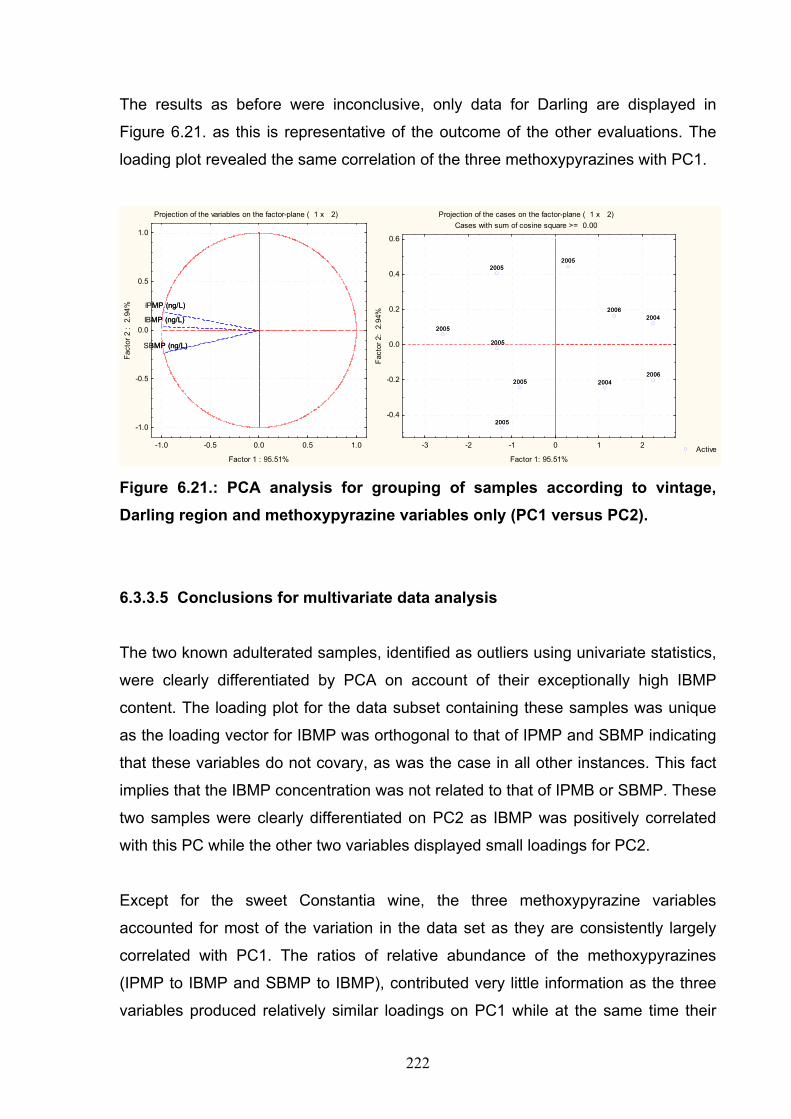
222

The results as before were inconclusive, only data for Darling are displayed in

Figure 6.21. as this is representative of the outcome of the other evaluations. The

loading plot revealed the same correlation of the three methoxypyrazines with PC1.


Active

MP (ng/L)

BMP (ng/L)

MP (ng/L)

-1.0 -0.5 0.0 0.5 1.0

Factor 1 : 95.51%

-1.0

-0.5

0.0

0.5

1.0

Fact

or 2

: 2

.94%

IBMP (ng/L)

SBMP (ng/L)

IPMP (ng/L)


Active

2004

2004

2005

20052005

2005

2005

2005

2006

2006

-3 -2 -1 0 1 2

Factor 1: 95.51%

-0.4

-0.2

0.0

0.2

0.4

0.6

Fact

or 2

: 2.

94%

2004

2004

2005

20052005

2005

2005

2005

2006

2006


Active

MP (ng/L)

BMP (ng/L)

MP (ng/L)

-1.0 -0.5 0.0 0.5 1.0

Factor 1 : 95.51%

-1.0

-0.5

0.0

0.5

1.0

Fact

or 2

: 2

.94%

IBMP (ng/L)

SBMP (ng/L)

IPMP (ng/L)


Active

2004

2004

2005

20052005

2005

2005

2005

2006

2006

-3 -2 -1 0 1 2

Factor 1: 95.51%

-0.4

-0.2

0.0

0.2

0.4

0.6

Fact

or 2

: 2.

94%

2004

2004

2005

20052005

2005

2005

2005

2006

2006

Figure 6.21.: PCA analysis for grouping of samples according to vintage, Darling region and methoxypyrazine variables only (PC1 versus PC2).

6.3.3.5 Conclusions for multivariate data analysis

The two known adulterated samples, identified as outliers using univariate statistics,

were clearly differentiated by PCA on account of their exceptionally high IBMP

content. The loading plot for the data subset containing these samples was unique

as the loading vector for IBMP was orthogonal to that of IPMP and SBMP indicating

that these variables do not covary, as was the case in all other instances. This fact

implies that the IBMP concentration was not related to that of IPMB or SBMP. These

two samples were clearly differentiated on PC2 as IBMP was positively correlated

with this PC while the other two variables displayed small loadings for PC2.

Except for the sweet Constantia wine, the three methoxypyrazine variables

accounted for most of the variation in the data set as they are consistently largely

correlated with PC1. The ratios of relative abundance of the methoxypyrazines

(IPMP to IBMP and SBMP to IBMP), contributed very little information as the three

variables produced relatively similar loadings on PC1 while at the same time their

223

contributions to PC2 was poor. Clear differentiation of the samples according to

region of origin utilizing PCA was not achieved. Considering that two extreme cases

(Constantia and Worcester) were only partially differentiated illustrates that other

production factors possibly play a far more determinative role in this regard. It was

similarly found that clear differentiation of the samples according to vintage was not

evident from PCA, even considering only samples form a specific region.

Stellenbosch, Constantia, Darling and Overberg were unsuccessfully evaluated for

possible differentiation according to vintage.

The loading plots for the data also revealed that the loading vectors for the three

methoxypyrazines and the other variables (alcohol and sugar content, total acidity

and pH) were in general consistently orthogonal indicating that the two sets of

variable are unrelated. As no covariance was thus observed, the time of harvesting

and phenological ripeness (that might manifest in a high total acidity for relatively

early harvesting4 and vice versa) does not appear to play a determinative role in the

methoxypyrazine content of the samples. The same general observation also

applies to the sugar content, which showed very little covariance with the

methoxypyrazine content of the sample (here a high sugar content may indicate

relative late harvesting resulting in lower wine methoxypyrazines).

It can be concluded that the significant variance in methoxypyrazine content and

ratios cannot unambiguously be ascribed to either geographical origin or vintage.

6.4. Conclusions

Two wines were identified as adulterated based on criteria that were developed in

this study. The Dixon Q-test test was applied to the data pertaining to the IBMP

concentration of the samples to demonstrate that the outliers were significantly

different from the population and that the deviations observed cannot be ascribed to

natural variance within the dataset. The ratios of abundance of IPMP and SBMP

relative to IBMP in the two adulterated products were also significantly lower than

those of the unadulterated samples. Although this difference could not statistically

be classified as significant, this phenomenon is consistent with adulteration of wine

224

with green pepper extracts or synthetic preparations. Results for the two adulterated

wines were confirmed utilizing PCA. The PCA loading plot revealed that with the two

adulterated wines, IBMP did not covary with IPMP and SBMP indicating that the

IBMP content in these samples were disproportionally high compared to

unadulterated samples.

Investigation of the data by PCA and Anova indicates that no clear grouping of

wines according to vintage or region of origin is evident. Knowledge of the vintage or

region of origin therefore provides very limited information for elucidation of

authenticity. As no clear correlation between the methoxypyrazine content and other

wines parameters (alcohol and reducing sugar content, total acidity and pH) were

observed, this also contributed no information regarding authenticity.

Unsuccessful classification of Sauvignon blanc wines may principally be attributed to

the wide variation in the 3-alkyl-2-methoxypyrazine concentration of the samples, a

phenomenon reported by various other authors.5,7,11,12,17 The concentration of these

components are reported to decline dramatically as ripening progress, more than

96% of the veraison level of IBMP was lost by normal harvesting maturity. Factors

associated with this decline include ripening temperature, viticultural conditions (soil

type, pruning and training, and plantation density) and light exposure .7,10,11,12,17

Regarding light exposure, it was postulated that the berry concentration of IBMP is

the result of two opposing effects, stimulation of biological formation on the one

hand and photodegradation on the other.17 It is also reported that IBMP mainly

resides in stems, skins and seeds in Cabernet Sauvignon grapes, while relatively

small amounts are located in the flesh. Although extractability was reported to play

minor role, prolonged skin contact resulted in significant increases of IBMP content

of juice.19 Settling is reported to have an equally dramatic influence on the IBMP

content of Sauvignon blanc must, clarification was reported to remove up to 50% of

IBMP.13,18 It may therefore be assumed that all the factors outlined above act

together in a complex manner so that the final 3-alkyl-2-methoxypyrazine

concentration of the samples are not simply the product of the vintage or region of

origin but rather an intricate combination of diverse factors.

225

Finally it should be noted that neither of the two strategies that were used can

provide absolute evidence of adulteration. As a very small amount of IBMP (1 to 2

ng/L) may have a significant effect on the aroma of Sauvignon blanc wine6,

manipulation of the aroma may be achieved by the addition of relatively small

quantities of IBMP to wine. Since the variation in the IBMP content, as well as in the

relative ratios, are relatively large in South African wines, the method may not be

able to detect cases of adulteration where small, measured amounts of adulterants

were added. Adulteration with small measured amounts may however not be easy

to achieve (without sophisticated equipment) because of the very low quantities, and

large volumes (of wine) involved. Synthetic preparations, where the

methoxypyrazine content may possibly be certified, may offer unscrupulous

producers an easy opportunity to manipulate the aroma of Sauvignon blanc wine

undetected.

226

REFERENCES



(2) C. du Plessis, GEURMIDDEL-SKADE GROOTLIKS ,BEPERK, Wineland,

(2005).

(3) J. Platter, SOUTH AFRICAN WINES 2007, The John Platter SA Wine Guide

(Pty) Ltd, P.O. Box 1466, Hermanus, 7200, 57 - 58.

(4) P. Hands, D. Hughes, WINES AND BRANDIES OF THE CAPE OF GOOD

HOPE, Stephan Phillips Publishers, 69.



WINES, Wynboer, (2004).

(6) M. S. Allen, M. J. Lacey, R. L. N. Harris, W. V. Brown, CONTRIBUTION OF

METHOXYPYRAZINES TO SAUVIGNON BLANC WINE AROMA, Am. J.

Enol. Vitic., 42 (1991), 109 - 112.


METHOXYPYRAZINES IN SAUVIGNON BLANC GRAPES AND WINE, Am.

J. Enol. Vitic., 42 (1991), 103 - 108.

(8) K. E. Murray, F. B. Whitfield, THE OCCURRENCE OF 3-ALKYL-2-

METHOXYPYRAZINES IN RAW VEGETABLES, J. Sci. Food. Agric., 26

(1975), 973 - 986.


METHOXYPYRAZINES IN RED WINES BY STABLE ISOTOPE DILUTION

GAS CHROMATOGRAPHY-MASS SPECTROMETRY, J. Agr. Food Chem.,

42 (1994), 1734 - 1738.

(10) J. Marais, FACTORS AFFECTING SAUVIGNON BLANC WINE QUALITY,

Wynboer, (2005), 69 - 70.

(11) D. Roujou De Boubee, C. Van Leeuwen, D. Dubourdieu, ORGANOLEPTIC

IMPACT OF 2-METHOXY-3-ISOBUTYLPYRAZINE ON RED BORDEAUX

AND LOIRE WINES, EFFECT OF ENVIRONMENTAL CONDITIONS ON

CONCENTRATIONS IN GRAPES DURING RIPENING, J. Agric. Food

Chem., 48 (2000), 4830 – 4834.

227

(12) C. Sala, O. Busto, J. Guasch, F. Zamora, INFLUENCE OF VINE TRAINING

AND SUNLIGHT EXPOSURE ON THE 3-ALKYL-2-METHOXYPYRAZINE

CONTENT IN MUSTS AND WINES FROM THE VITIS VINIFERA VARIETY

CABERNET SAUVIGNON, J. Agr. Food Chem., 52 (2004), 3492 – 3497.

(13) D. Roujou de Boubee, RESEARCH ON 2-METHOXY-3-

ISOBUTYLPYRAZINE IN GRAPES AND WINE, School of Oenology,

University of Bordeaux II.

(14) D. A. Skoog, F. J. Holler, T. A. Nieman, PRINCIPLES OF INSTRUMENTAL

ANALYSIS, 5th ed. (1998), Saunders College Publishing, Philadelphia, 11 -

68.

(15) K. H. Esbensen, MULTIVARIATE DATA ANALYSIS IN PRACTICE, 5th ed.

(2002), CAMO Process AS, Nedre Vollgate 8, N-0158 Oslo, Norway, 1 - 97.

(16) B. G. M. Vandeginste, D. L. Massart, L. M. C. Buydens, et al., HANDBOOK

OF CHEMOMETRICS AND QUALIMETRICS, Part B, (1997), Elsevier.


AFFECT BERRY METHOXYPYRAZINE CONCENTRATION, Am. J. Enol.

Vitic., 50 (1999), 194 - 198.

(16) D. Roujou De Boubee, A. M. Cumsille, M. Pons, D. Dubourdieu, LOCATION

OF 2-METHOXY-3-ISOBUTYLPYRAZINE IN CABERNET SAUVIGNON

GRAPE BUNCHES AND ITS EXTRACTABILITY DURING VINIVICATION,

Am. J. Enol. Vitic., 53 (2002), 1 – 5.

(19) M. Maggu, R. Winz, P.A. Kilmartin, M.C.T. Trought, L. Nicolau, EFFECT OF

SKIN CONTACT AND PRESSURE ON THE COMPOSITION OF

SAUVIGNON BLANC MUST, J.Agric. Food Chem., 55 (2007), 10281 –

10288.

CHAPTER 7

Summary and final concluding remarks

The South African Sauvignon blanc industry was under intense scrutiny for a

number of years regarding adulteration of wines with foreign sources of 3-alkyl-2-

methoxypyrazines.1 In 2004, following an investigation conducted by the Wine and

Spirit Board and the Agricultural Research Council (ARC Nietvoorbij), two producers

admitted that illegal flavorants were added to their wines. The total volume of

production of the relevant products were subsequently destroyed.2 As adulteration

constitutes a transgression of the Liquor Products Act3, official samples of the

contaminated products were confiscated by officials from the National Department of

Agriculture while details of the case were passed on to the National Prosecuting

Authority for consideration of possible legal action.

Regulation of the South African wine industry is a function that resorts under the

National Department of Agriculture. As adulteration may tarnish the image of South

African wines in the international market place and jeopardize the market share that

South African producers command, it was decided that an extensive audit of the

industry should be performed as a matter of the utmost urgency. Furthermore it was

required that the two cases of adulteration be investigated and that evidence should

be prepared to support possible litigation in this regard.

Within this context, the objectives of the study were two-fold in nature: Firstly a

methodology for the determination of 3-alkyl-2-methoxypyrazines in South African

Sauvignon blanc wines was developed and implemented (Chapters 3, 4 and 5), and

secondly a spectrum of wines representative of the industry were analyzed to

establish parameters for authenticity elucidation and to perform an extensive audit of

the industry (Chapter 6) at the same time. A comprehensive database of the 3-alkyl-

2-methoxypyrazine content (Appendix 2, Table A) of South African Sauvignon blanc

wines was thus established to provide information to enable the industry audit.

Supplementary information yielded by possible sources of adulteration namely

229

green peppers and synthetic green pepper preparations, were also obtained in order

to predict the effect of the addition thereof to wine. A small number of wines of other

cultivars (Appendix 2, Table B) as well as Sauvignon blanc leaves were also

analyzed.

Liquid chromatography-mass spectrometry (LC-MS) was selected as the analytical

technique for measuring the levels of 3-alkyl-2-methoxypyrazines. The described

method, utilizing distillation and solvent extraction for sample clean-up and pre-

concentration followed by LC-MS determination of the residues, offered enhanced

sensitivity compared to other techniques that were used for the same purpose. The

method performance mostly allowed determination of the 3-alkyl-2-

methoxypyrazines in South African Sauvignon blanc wines at their natural levels of

occurrence. Table 7.1. summarize some of the performance characteristics of the

method.

Table 7.1.: Performance characteristics of the method utilized for determination of 3-alkyl-2-methoxypyrazines in South African Sauvignon blanc wine.

Parameter Value MDL 0.03 ng/L MQL 0.10 ng/L Linear system response Demonstrated for 5 to 4000 pg on column for IBMP

and 5 to 1000 pg on column for IPMP and SBMP. Recovery Better than 90% (RSD < 10%) at levels 1, 10 and 100

ng/L Instrument precision RSD better than 5% utilizing aqueous standards. Specificity Molecular ion and one ion ratio for two secondary ion

transitions were obtained.

The method described in this work represents the first known instance where LC-MS

was applied for trace-level quantitation of 3-alkyl-2-methoxypyrazines in wine. The

method produced improved levels of sensitivity compared to GC methods used for

the same purpose and was successfully used to generate the most complete

database pertaining to the 3-alkyl-2-methoxypyrazine content of South African

Sauvignon blanc wine to date. The improved sensitivity realized with the method

enabled the authors to quantify IBMP in all samples investigated as well as IPMP

and SBMP in the majority of cases. The IBMP content was also measured in a

230

number of wines of other cultivars including for the first known instance in Pinotage,

a unique South African cultivar. The improved sensitivity attained with the method

therefore opens possibilities to study these components in wines which previously

contained them in levels that were below the capabilities of known techniques.

A total of 577 South African Sauvignon blanc wines, from all wine-producing regions

and of vintages 1999 to 2007, were analyzed. Due to sample availability constraints,

only the 2004 and 2005 vintages were well represented with 197 and 295 samples

respectively. Sauvignon blanc wines are mainly produced in the Breede River Valley

and Coastal regions and as 118 and 268 samples were from these respective

regions, sampling may be considered as reasonably representative regarding

geographical origin of the wines.

Measured values for the IBMP concentration in this study ranged from 0.40 to 44

ng/L (RSD = 102%) with an average of 6.2 ng/L and median of 4.3 ng/L indicating

that the distribution of values are not symmetrical, the majority of the samples were

at the lower end of the scale. The concentrations of IPMP and SBMP in South

African Sauvignon blanc wines were consistently lower than that of IBMP, and

ranged from < 0.03 to 3.9 ng/L and < 0.03 to 3.2 ng/L respectively. The ratios of

IPMP to IBMP, and SBMP to IBMP were determined to be approximately 5% in

each case. The analysis of green peppers revealed that IBMP is similarly the

dominant 3-alkyl-2-methoxypyrazine as was the case with the synthetic flavor

preparations. However, the relative abundances of IPMP and SBMP were generally

far smaller in these items compared to Sauvignon blanc wine. Two criteria were

therefore identified that may be used for authenticity elucidation; the absolute

concentration of IBMP, and the ratios of IPMP to IBMP and SBMP to IBMP.

The data was also analyzed to determine whether factors such as the

methoxypyrazine content and other wine parameters (alcohol and reducing sugar

content, total acidity and pH) may be correlated with the region of origin or vintage of

the samples. Data analysis was performed using univariate statistics as well as

PCA. The results revealed that only a superficial relationship between the 3-alkyl-2-

methoxypyrazine content of the samples and some regions of origin could be

established. No correlation with the vintage or any of the other wine parameters

231

could be established. Rigid parameters could therefore not be established for the

elucidation of authenticity, the factors discussed above should be considered

together to establish authenticity. The method was nevertheless able to discriminate

the two adulterated samples based on disproportionately high levels of IBMP.

The two adulterated samples contained statistically significant elevated levels of

IBMP while the ratios of abundance of IPMP and SBMP were consistent with

adulteration. No additional cases of adulteration in the dataset were identified based

on the said criteria, a finding that may serve to restore confidence in the wine

industry as it would certainly appear that adulteration is not as widespread as it was

at first assumed to be. In this regard it should be noted that the suspicion is that

adulteration mainly took place in vintages earlier than 2004. Although a limited

number of samples of these relatively early vintages were available, these revealed

no indication of adulteration as discussed above. Where small, but significant (only 1

to 2 ng/L IBMP required to influence wine aroma) amounts of adulterants may have

been added, the method could clearly not detect the duplicity. From a practical

perspective, the addition of small amounts of methoxypyrazines to large volumes of

wine to affect enrichment at levels that does not exceed the natural abundance, may

be difficult to achieve without sophisticated equipment.

From the data it is also evident that it certainly is possible to produce Sauvignon

blanc wine in South Africa that posses the desired and characteristic herbaceous

aroma. A total of 82% of the samples contained IBMP above the perceptible level in

white wine (2 ng/L) while 16% of the products contained more that 10 ng/L IBMP.

Further research in the viticultural field may reveal the factors that contribute to the

high levels of IBMP observed in some wines and possibly facilitate the production of

wines with consistently high levels. Future method developments regarding

detection of adulteration may possibly focus on other substances unique to green

peppers and synthetic preparations (but not wine) that might be added to wine as a

result of the adulteration process. However, such components if present at all would

almost certainly be present at very low concentrations. The probability that a natural

component of this nature, present at ultra-trace levels will be unique to green

peppers and not to wine may be small. This method is therefore currently the only

available option to determine adulteration of this nature and as it utilizes two sets of

232

parameters for authenticity elucidation, it represents an improvement on similar

strategies utilized for the same purpose.

233

REFERENCES

(1) DIE BURGER, 14 February 2004.

(2) C. du Plessis, GEURMIDDEL-SKADE GROOTLIKS BEPERK, Wineland,

(2005).



Appendix 1: Mass spectra of components of interest

3-Methyl-2-methoxypyrazine

3-Ethyl-2-methoxypyrazine

m/z 50 60 70 80 90 100 110 120 130 140 150 160 170 180 190 200

%

0

100

124.04

111.03

138.87

m/z 50 60 70 80 90 100 110 120 130 140 150 160

%

0

100

56.17

125.02

96.99

235

3-Isopropyl-2-methoxypyrazine

3-Isobutyl-2-methoxypyrazine

m/z 50 60 70 80 90 100 110 120 130 140 150 160 170 180 190 200 210 220

%

0

100

123.98

166.98

124.98

m/z 50 60 70 80 90 100 110 120 130 140 150 160 170 180 190 200

%

0

100

137.87

122.97

152.90

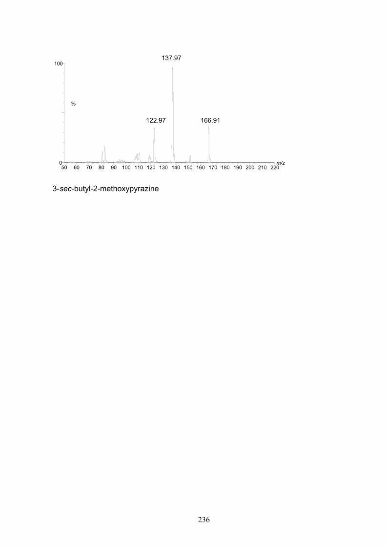
236

3-sec-butyl-2-methoxypyrazine

m/z 50 60 70 80 90 100 110 120 130 140 150 160 170 180 190 200 210 220

%

0

100 137.97

122.97

166.91

Appendix 2: Quantitative data for wines analyzed in the study Table A: Data pertaining to Sauvignon blanc wine (main study). No. Origin Vintage IBMP(ng/L) SBMP(ng/L) IPMP(ng/L) IPMP(%) SBMP(%) Alc(%v/v) Sug(g/L) pH T.A.(g/L) 1 Western Cape 2004 3.9 0.16 0.19 4.9 4.1 12.62 1.4 3.24 6.4 2 Western Cape 2004 4.8 0.22 0.15 3.1 4.6 12.23 1.6 3.58 6.0 3 Franschhoek 2004 0.82 NQ ND - - 13.49 3.3 3.09 7.3 4 Franschhoek 2004 1.1 NQ ND - - 13.41 1.3 3.05 7.1 5 Paarl 2004 4.6 0.18 0.16 3.5 3.9 15.10 1.3 3.49 4.9 6 Stellenbosch 2005 11 0.24 0.63 5.7 2.2 13.32 1.7 3.38 6.0 7 Stellenbosch 2002 2.5 NQ 0.13 5.2 - 13.32 2.5 3.19 6.0 8 Western Cape 2003 6.9 0.12 ND - 1.7 12.71 1.5 3.36 5.8 9 Western Cape 2003 1.2 NQ ND - - 13.41 1.5 3.35 7.3 10 Wellington 2004 6.9 0.25 0.67 9.7 3.6 12.28 2.5 3.19 6.3 11 Stellenbosch 2002 2.2 0.11 NQ - 5.0 13.32 1.3 3.71 5.8 12 Western Cape 2004 3.2 0.12 NQ - 3.8 12.62 4.2 3.28 6.8 13 Coastal region 2005 3.2 NQ 0.21 6.6 - 12.88 4.7 2.97 6.8 14 Coastal region 2005 3.4 0.12 0.11 3.2 3.5 12.88 4.7 2.97 6.8 15 Wellington 2005 1.6 ND ND - - 11.76 5.3 3.36 7.0 16 Groenekloof 2005 15 0.47 1.3 8.4 3.1 12.71 1.3 3.39 7.3 17 Stellenbosch 2005 4.3 ND NQ - - 13.49 1.7 3.07 7.1 18 Coastal region 2004 310 0.12 0.68 0.2 0.0 19 n/o 2004 960 0.14 0.69 0.1 0.0 20 Constantia 2004 18 0.40 1.1 6.1 2.2 12.97 1.6 3.38 6.9 21 Stellenbosch 2004 2.1 NQ NQ - - 13.14 1.6 3.20 6.3 22 Coastal region 2004 8.7 0.30 0.64 7.4 3.4 13.06 1.3 3.17 6.6 23 Stellenbosch 2004 5.2 0.18 0.30 5.8 3.5 12.88 2.4 3.43 6.8 24 Western Cape 2003 1.6 NQ NQ - - 13.36 1.7 3.19 6.5 25 Western Cape 2004 2.8 0.13 NQ - 4.6 13.94 2.4 3.32 6.0 26 Constantia 2004 12 0.25 0.85 7.1 2.1 12.97 3.3 3.25 7.5 27 Western Cape 2004 4.7 0.16 0.63 13.4 3.4 13.37 2.7 3.80 4.8 28 Paarl 2003 3.1 0.10 0.14 4.5 3.2 12.88 1.4 3.44 4.9 29 Stellenbosch 2004 2.1 NQ NQ - - 13.53 1.7 3.11 5.9 30 Swartland 2004 3.6 ND 0.11 3.1 - 12.19 1.6 3.48 5.9 31 Tulbagh 2004 2.2 0.12 ND - 5.5 12.97 2.9 2.93 6.9 32 Coastal region 2005 18 0.29 1.0 5.6 1.6 13.23 1.8 3.47 6.9

238

No. Origin Vintage IBMP(ng/L) SBMP(ng/L) IPMP(ng/L) IPMP(%) SBMP(%) Alc(%v/v) Sug(g/L) pH T.A.(g/L) 33 Western Cape 2004 8.4 0.19 0.41 4.9 2.3 12.02 3.2 3.57 5.6 34 Robertson 2004 3.1 0.13 0.18 5.8 4.2 12.49 1.0 3.34 6.4 35 Robertson 2004 25 0.38 1.3 5.0 1.5 12.83 1.4 3.62 7.6 36 Robertson 2004 3.2 0.18 0.11 3.4 5.6 12.80 1.6 3.45 6.4 38 Robertson 2004 1.6 0.10 ND - 6.3 13.76 3.1 3.36 6.7 39 Robertson 2004 1.7 0.10 ND - 5.9 13.72 2.8 3.31 6.6 40 Worcester 2003 1.4 0.13 ND - 9.3 13.21 7.5 3.43 6.5 41 Worcester 2002 2.2 0.15 ND - 6.8 12.70 5.8 3.07 7.8 42 Slanghoek 2003 20 0.30 0.88 4.4 1.5 12.39 1.1 3.19 7.2 43 Breëriviervallei 2003 1.5 NQ NQ - - 13.77 1.4 3.32 5.3 44 Goudini 2003 5.4 0.21 0.11 2.0 3.9 12.90 1.0 3.19 6.1 45 Robertson 2004 2.3 0.13 0.24 10.4 5.7 12.49 1.1 3.57 5.4 46 Robertson 2004 1.7 NQ NQ - - 13.98 2.9 3.30 6.6 47 Robertson 2004 1.8 0.10 NQ - 5.6 13.60 2.3 3.62 6.4 48 Worcester 2003 1.3 0.10 ND - 7.7 13.19 2.3 3.42 6.8 49 Worcester 2003 2.5 0.15 0.17 6.8 6.0 12.25 1.2 3.46 5.8 50 Breëriviervallei 2003 0.72 NQ NQ - - 13.19 1.4 3.16 5.8 51 Robertson 2004 0.66 NQ NQ - - 13.01 1.3 3.20 5.9 52 Robertson 2004 3.2 0.20 0.17 5.3 6.3 11.93 1.3 3.39 7.5 53 Robertson 2004 24 0.31 1.3 5.5 1.3 12.45 1.3 3.58 8.0 54 Robertson 2004 5.7 0.17 0.17 3.0 3.0 12.38 2.0 3.49 8.0 56 Robertson 2003 1.9 0.13 NQ - 6.8 12.01 1.4 3.60 6.4 57 Robertson 2004 3 0.12 NQ - 4.0 12.10 1.2 3.11 6.2 58 Worcester 2002 1.8 0.13 NQ - 7.2 12.93 2.7 3.41 6.3 59 Worcester 2003 2.7 0.26 0.11 4.1 9.6 13.41 7.2 3.11 7.0 60 Breëriviervallei 2002 1.7 0.13 0.12 7.1 7.6 12.63 2.6 3.46 6.4 61 Worcester 2003 3.1 0.36 0.10 3.2 11.6 13.07 9.4 3.18 7.1 62 Goudini 2003 5.8 0.24 0.33 5.7 4.1 12.94 3.6 3.18 6.2 63 Worcester 2002 16 0.46 0.19 1.2 2.9 12.78 1.2 3.53 5.0 64 Goudini 2003 3.6 0.13 NQ - 3.6 11.48 1.0 3.50 6.9 65 Worcester 2003 6 0.22 0.23 3.8 3.7 11.59 1.1 3.57 6.8 66 Worcester 2003 11 0.11 0.23 2.1 1.0 11.41 1.1 3.41 7.0 67 Worcester 2003 2.8 0.29 NQ - 10.4 13.33 7.8 3.16 6.6 68 Worcester 2003 3.2 0.18 0.10 3.1 5.6 11.10 1.0 3.59 7.0 69 Worcester 2003 2.3 0.10 NQ - 4.3 10.79 1.3 3.28 6.3 70 Worcester 2004 5.1 0.29 0.25 4.9 5.7 12.67 1.6 3.34 6.5

239

No. Origin Vintage IBMP(ng/L) SBMP(ng/L) IPMP(ng/L) IPMP(%) SBMP(%) Alc(%v/v) Sug(g/L) pH T.A.(g/L) 71 Nuy 2004 5.9 0.23 0.36 6.1 3.9 12.97 1.3 3.36 7.0 72 Nuy 2004 4.5 0.19 0.22 4.9 4.2 13.14 1.8 3.29 6.6 73 Goudini 2004 11 0.28 0.62 5.6 2.5 13.14 5.1 3.33 7.4 74 Worcester 2004 3 0.17 0.28 9.3 5.7 12.19 1.4 3.25 6.4 75 Worcester 2004 4.3 0.12 NQ - 2.8 12.31 3.3 3.20 5.8 76 Slanghoek 2004 11 0.31 0.96 8.7 2.8 11.81 4.2 3.37 7.6 77 Worcester 2004 6.1 0.21 0.23 3.8 3.4 12.10 1.0 3.46 6.1 78 Worcester 2004 2.8 0.19 0.21 7.5 6.8 12.19 3.0 3.29 6.3 80 Worcester 2004 4.6 0.39 0.22 4.8 8.5 12.40 3.9 3.61 7.3 81 Worcester 2004 5.4 0.16 0.17 3.1 3.0 12.62 2.0 3.49 6.5 82 Robertson 2004 3.9 0.14 NQ - 3.6 11.34 1.4 3.41 6.4 83 Robertson 2004 25 0.44 1.1 4.4 1.8 12.31 1.5 3.53 7.4 84 Robertson 2004 1.2 NQ NQ - - 13.36 2.8 3.13 6.9 86 Robertson 2004 11 0.26 0.24 2.2 2.4 13.30 1.3 3.39 5.7 87 Robertson 2004 3.9 0.10 0.15 3.8 2.6 12.16 4.6 3.31 7.1 88 Robertson 2004 4.6 0.11 0.44 9.6 2.4 11.88 1.4 3.40 6.7 89 Robertson 2004 3.8 0.18 0.21 5.5 4.7 12.05 1.0 3.07 5.8 90 Robertson 2004 2.7 0.16 NQ - 5.9 13.46 2.7 3.30 7.8 91 Bonnievale 2004 4.6 0.18 0.48 10.4 3.9 12.49 3.5 3.25 6.9 92 Robertson 2004 2.8 0.18 0.13 4.6 6.4 12.45 1.4 3.33 6.5 93 Robertson 2004 11 0.30 0.60 5.5 2.7 11.62 2.0 3.19 6.5 94 Western Cape 2004 8.3 0.12 0.30 3.6 1.4 12.19 3.2 3.21 7.1 95 Western Cape 2004 4.2 0.15 0.22 5.2 3.6 12.71 1.3 3.33 6.9 96 Constantia 2005 20 3.2 2.6 12.9 15.8 13.58 2.6 3.25 6.3 97 Prince Albert Valley 2005 4.2 0.16 NQ - 3.8 12.19 6.0 3.26 6.2 98 Robertson 2004 2.3 0.15 NQ - 6.5 13.42 1.3 3.76 5.3 99 Robertson 2004 17 0.46 1.2 7.1 2.7 11.59 1.9 3.38 7.1 100 McGregor 2004 5.4 0.44 0.76 14.1 8.1 12.02 2.7 3.43 6.3 101 Robertson 2004 1.5 NQ ND - - 12.10 1.4 3.21 6.2 103 Robertson 2004 5.3 0.21 0.27 5.1 4.0 12.56 1.5 3.52 7.6 104 Robertson 2004 2.7 0.18 0.23 8.5 6.7 12.80 1.5 3.44 6.4 105 McGregor 2004 4.1 0.36 0.40 9.8 8.8 12.02 3.2 3.30 6.8 106 Robertson 2004 2.8 0.20 0.13 4.6 7.1 12.80 1.6 3.45 6.4 107 Robertson 2004 5.1 0.22 0.45 8.8 4.3 12.28 3.0 3.52 6.5 108 Robertson 2004 1 0.13 NQ - 13.0 13.49 2.8 3.25 6.7 109 McGregor 2004 1.7 0.24 0.15 8.8 14.1 12.31 3.4 3.33 6.2

240

No. Origin Vintage IBMP(ng/L) SBMP(ng/L) IPMP(ng/L) IPMP(%) SBMP(%) Alc(%v/v) Sug(g/L) pH T.A.(g/L) 110 Robertson 2004 24 0.45 1.6 6.8 1.9 12.66 1.3 3.56 7.7 111 Goudini 2004 4.4 0.18 0.27 6.1 4.1 12.31 1.1 3.33 6.4 112 Worcester 2004 5.8 0.23 0.29 5.0 4.0 12.14 1.0 3.44 5.7 113 Robertson 2004 1.4 0.13 NQ - 9.3 12.14 1.1 3.50 5.7 114 Nuy 2003 2 0.16 NQ - 8.0 12.46 1.6 3.21 6.4 115 Slanghoek 2003 17 0.22 0.22 1.3 1.3 12.36 3.0 3.28 7.3 116 Worcester 2003 2.5 0.15 NQ - 6.0 12.50 1.2 3.45 5.8 117 Worcester 2003 2.3 0.15 0.19 8.3 6.5 13.15 3.2 3.32 6.0 118 Goudini 2003 4.1 0.22 0.22 5.4 5.4 12.51 2.4 3.36 5.8 119 Goudini 2003 4.9 0.18 0.26 5.3 3.7 12.78 1.7 3.40 5.6 120 Breëriviervallei 2003 1.3 0.10 NQ - 7.7 13.83 2.5 3.43 6.8 121 Breëriviervallei 2003 1.3 0.13 0.10 7.7 10.0 13.49 1.2 3.39 7.0 122 Slanghoek 2004 10 0.31 0.91 9.1 3.1 11.76 1.2 3.45 6.7 123 Slanghoek 2004 26 0.78 3.3 12.8 3.0 13.98 1.5 3.27 6.0 124 Worcester 2004 6.3 0.37 0.54 8.6 5.9 11.53 1.4 3.38 6.3 125 Goudini 2004 9.3 0.24 0.52 5.6 2.6 11.10 2.9 3.71 5.7 126 Worcester 2004 3.1 0.23 0.24 7.7 7.4 11.79 1.5 3.39 5.9 127 Worcester 2004 17 0.56 0.73 4.3 3.3 11.79 1.2 3.44 6.7 128 Worcester 2004 3.1 0.14 0.17 5.5 4.5 13.25 1.2 3.36 6.3 129 Worcester 2004 4.7 0.27 0.32 6.8 5.7 12.75 3.8 3.59 5.8 130 Worcester 2004 4 0.25 0.22 5.5 6.3 12.75 3.3 3.48 5.9 131 Goudini 2004 5.7 0.15 NQ - 2.6 11.09 1.3 3.51 6.4 132 Nuy 2004 5.6 0.26 0.25 4.5 4.6 12.49 2.7 3.32 6.6 133 Nuy 2004 5.9 0.27 0.21 3.6 4.6 12.66 1.1 3.22 7.8 134 Worcester 2003 2.8 0.33 0.11 3.9 11.8 13.08 2.0 3.28 6.1 135 Worcester 2003 1.9 0.30 0.12 6.3 15.8 13.36 5.0 3.28 6.4 137 Worcester 2003 9.4 0.20 0.19 2.0 2.1 13.15 2.6 3.41 6.2 138 Robertson 2004 2.3 0.17 0.17 7.4 7.4 11.09 1.1 3.40 7.1 139 Worcester 2003 2.6 0.17 0.31 11.9 6.5 13.03 3.8 3.28 6.8 140 Robertson 2004 1 0.15 NQ - 15.0 12.28 2.8 3.36 6.4 141 Goudini 2003 2.5 0.22 NQ - 8.8 13.26 1.5 3.39 6.5 142 Goudini 2003 2.7 0.19 0.11 4.1 7.0 13.27 1.0 3.51 5.8 143 Robertson 2004 2.7 0.21 0.12 4.4 7.8 12.88 3.3 3.48 5.7 145 Goudini 2003 4.4 0.30 0.18 4.1 6.8 12.18 1.3 3.28 7.4 146 Tradouw 2003 1.4 0.15 0.12 8.6 10.7 13.67 2.2 3.43 5.1 147 Coastal region 2003 18 0.28 0.20 1.1 1.6 12.62 2.7 3.44 5.9

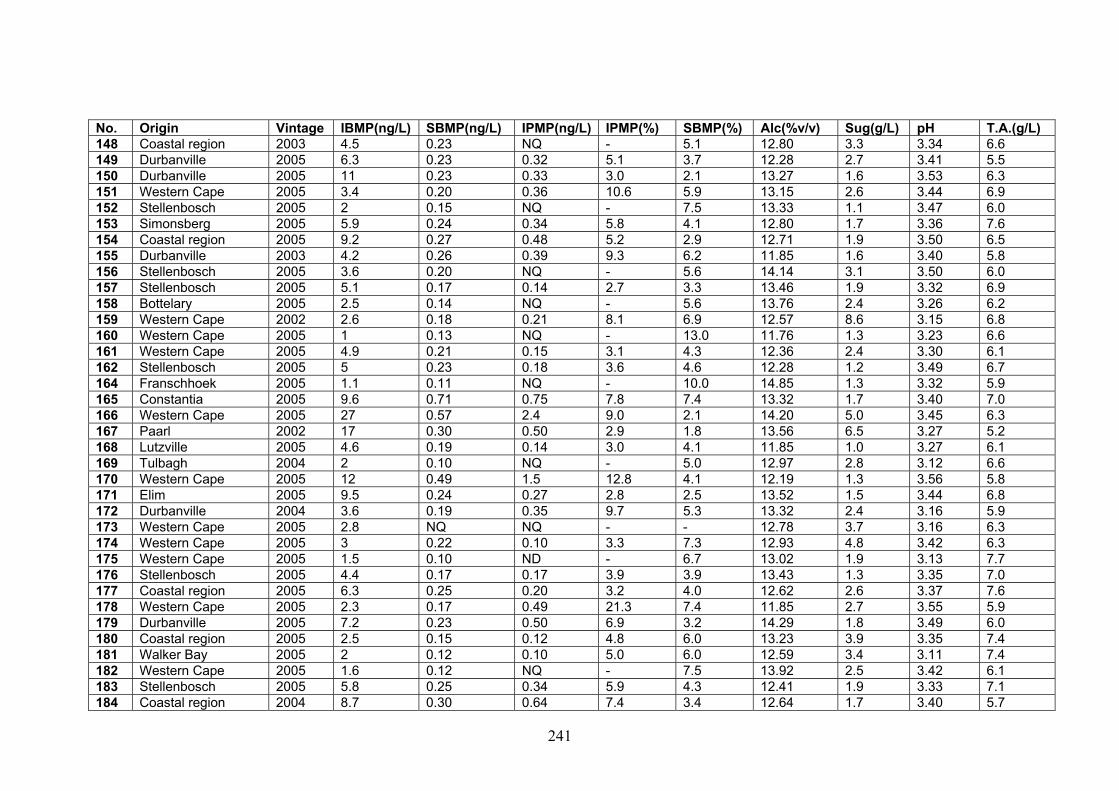
241

No. Origin Vintage IBMP(ng/L) SBMP(ng/L) IPMP(ng/L) IPMP(%) SBMP(%) Alc(%v/v) Sug(g/L) pH T.A.(g/L) 148 Coastal region 2003 4.5 0.23 NQ - 5.1 12.80 3.3 3.34 6.6 149 Durbanville 2005 6.3 0.23 0.32 5.1 3.7 12.28 2.7 3.41 5.5 150 Durbanville 2005 11 0.23 0.33 3.0 2.1 13.27 1.6 3.53 6.3 151 Western Cape 2005 3.4 0.20 0.36 10.6 5.9 13.15 2.6 3.44 6.9 152 Stellenbosch 2005 2 0.15 NQ - 7.5 13.33 1.1 3.47 6.0 153 Simonsberg 2005 5.9 0.24 0.34 5.8 4.1 12.80 1.7 3.36 7.6 154 Coastal region 2005 9.2 0.27 0.48 5.2 2.9 12.71 1.9 3.50 6.5 155 Durbanville 2003 4.2 0.26 0.39 9.3 6.2 11.85 1.6 3.40 5.8 156 Stellenbosch 2005 3.6 0.20 NQ - 5.6 14.14 3.1 3.50 6.0 157 Stellenbosch 2005 5.1 0.17 0.14 2.7 3.3 13.46 1.9 3.32 6.9 158 Bottelary 2005 2.5 0.14 NQ - 5.6 13.76 2.4 3.26 6.2 159 Western Cape 2002 2.6 0.18 0.21 8.1 6.9 12.57 8.6 3.15 6.8 160 Western Cape 2005 1 0.13 NQ - 13.0 11.76 1.3 3.23 6.6 161 Western Cape 2005 4.9 0.21 0.15 3.1 4.3 12.36 2.4 3.30 6.1 162 Stellenbosch 2005 5 0.23 0.18 3.6 4.6 12.28 1.2 3.49 6.7 164 Franschhoek 2005 1.1 0.11 NQ - 10.0 14.85 1.3 3.32 5.9 165 Constantia 2005 9.6 0.71 0.75 7.8 7.4 13.32 1.7 3.40 7.0 166 Western Cape 2005 27 0.57 2.4 9.0 2.1 14.20 5.0 3.45 6.3 167 Paarl 2002 17 0.30 0.50 2.9 1.8 13.56 6.5 3.27 5.2 168 Lutzville 2005 4.6 0.19 0.14 3.0 4.1 11.85 1.0 3.27 6.1 169 Tulbagh 2004 2 0.10 NQ - 5.0 12.97 2.8 3.12 6.6 170 Western Cape 2005 12 0.49 1.5 12.8 4.1 12.19 1.3 3.56 5.8 171 Elim 2005 9.5 0.24 0.27 2.8 2.5 13.52 1.5 3.44 6.8 172 Durbanville 2004 3.6 0.19 0.35 9.7 5.3 13.32 2.4 3.16 5.9 173 Western Cape 2005 2.8 NQ NQ - - 12.78 3.7 3.16 6.3 174 Western Cape 2005 3 0.22 0.10 3.3 7.3 12.93 4.8 3.42 6.3 175 Western Cape 2005 1.5 0.10 ND - 6.7 13.02 1.9 3.13 7.7 176 Stellenbosch 2005 4.4 0.17 0.17 3.9 3.9 13.43 1.3 3.35 7.0 177 Coastal region 2005 6.3 0.25 0.20 3.2 4.0 12.62 2.6 3.37 7.6 178 Western Cape 2005 2.3 0.17 0.49 21.3 7.4 11.85 2.7 3.55 5.9 179 Durbanville 2005 7.2 0.23 0.50 6.9 3.2 14.29 1.8 3.49 6.0 180 Coastal region 2005 2.5 0.15 0.12 4.8 6.0 13.23 3.9 3.35 7.4 181 Walker Bay 2005 2 0.12 0.10 5.0 6.0 12.59 3.4 3.11 7.4 182 Western Cape 2005 1.6 0.12 NQ - 7.5 13.92 2.5 3.42 6.1 183 Stellenbosch 2005 5.8 0.25 0.34 5.9 4.3 12.41 1.9 3.33 7.1 184 Coastal region 2004 8.7 0.30 0.64 7.4 3.4 12.64 1.7 3.40 5.7

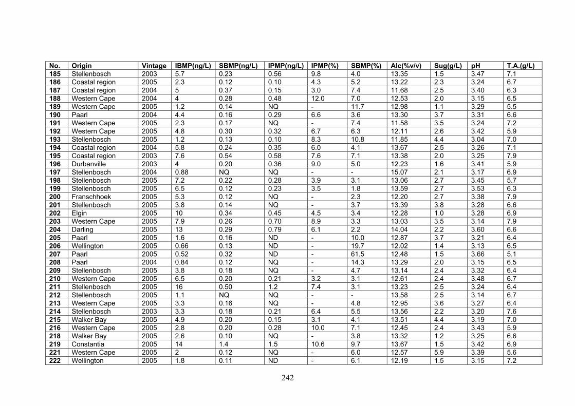
242

No. Origin Vintage IBMP(ng/L) SBMP(ng/L) IPMP(ng/L) IPMP(%) SBMP(%) Alc(%v/v) Sug(g/L) pH T.A.(g/L) 185 Stellenbosch 2003 5.7 0.23 0.56 9.8 4.0 13.35 1.5 3.47 7.1 186 Coastal region 2005 2.3 0.12 0.10 4.3 5.2 13.22 2.3 3.24 6.7 187 Coastal region 2004 5 0.37 0.15 3.0 7.4 11.68 2.5 3.40 6.3 188 Western Cape 2004 4 0.28 0.48 12.0 7.0 12.53 2.0 3.15 6.5 189 Western Cape 2005 1.2 0.14 NQ - 11.7 12.98 1.1 3.29 5.5 190 Paarl 2004 4.4 0.16 0.29 6.6 3.6 13.30 3.7 3.31 6.6 191 Western Cape 2005 2.3 0.17 NQ - 7.4 11.58 3.5 3.24 7.2 192 Western Cape 2005 4.8 0.30 0.32 6.7 6.3 12.11 2.6 3.42 5.9 193 Stellenbosch 2005 1.2 0.13 0.10 8.3 10.8 11.85 4.4 3.04 7.0 194 Coastal region 2004 5.8 0.24 0.35 6.0 4.1 13.67 2.5 3.26 7.1 195 Coastal region 2003 7.6 0.54 0.58 7.6 7.1 13.38 2.0 3.25 7.9 196 Durbanville 2003 4 0.20 0.36 9.0 5.0 12.23 1.6 3.41 5.9 197 Stellenbosch 2004 0.88 NQ NQ - - 15.07 2.1 3.17 6.9 198 Stellenbosch 2005 7.2 0.22 0.28 3.9 3.1 13.06 2.7 3.45 5.7 199 Stellenbosch 2005 6.5 0.12 0.23 3.5 1.8 13.59 2.7 3.53 6.3 200 Franschhoek 2005 5.3 0.12 NQ - 2.3 12.20 2.7 3.38 7.9 201 Stellenbosch 2005 3.8 0.14 NQ - 3.7 13.39 3.8 3.28 6.6 202 Elgin 2005 10 0.34 0.45 4.5 3.4 12.28 1.0 3.28 6.9 203 Western Cape 2005 7.9 0.26 0.70 8.9 3.3 13.03 3.5 3.14 7.9 204 Darling 2005 13 0.29 0.79 6.1 2.2 14.04 2.2 3.60 6.6 205 Paarl 2005 1.6 0.16 ND - 10.0 12.87 3.7 3.21 6.4 206 Wellington 2005 0.66 0.13 ND - 19.7 12.02 1.4 3.13 6.5 207 Paarl 2005 0.52 0.32 ND - 61.5 12.48 1.5 3.66 5.1 208 Paarl 2004 0.84 0.12 NQ - 14.3 13.29 2.0 3.15 6.5 209 Stellenbosch 2005 3.8 0.18 NQ - 4.7 13.14 2.4 3.32 6.4 210 Western Cape 2005 6.5 0.20 0.21 3.2 3.1 12.61 2.4 3.48 6.7 211 Stellenbosch 2005 16 0.50 1.2 7.4 3.1 13.23 2.5 3.24 6.4 212 Stellenbosch 2005 1.1 NQ NQ - - 13.58 2.5 3.14 6.7 213 Western Cape 2005 3.3 0.16 NQ - 4.8 12.95 3.6 3.27 6.4 214 Stellenbosch 2003 3.3 0.18 0.21 6.4 5.5 13.56 2.2 3.20 7.6 215 Walker Bay 2005 4.9 0.20 0.15 3.1 4.1 13.51 4.4 3.19 7.0 216 Western Cape 2005 2.8 0.20 0.28 10.0 7.1 12.45 2.4 3.43 5.9 218 Walker Bay 2005 2.6 0.10 NQ - 3.8 13.32 1.2 3.25 6.6 219 Constantia 2005 14 1.4 1.5 10.6 9.7 13.67 1.5 3.42 6.9 221 Western Cape 2005 2 0.12 NQ - 6.0 12.57 5.9 3.39 5.6 222 Wellington 2005 1.8 0.11 ND - 6.1 12.19 1.5 3.15 7.2

243

No. Origin Vintage IBMP(ng/L) SBMP(ng/L) IPMP(ng/L) IPMP(%) SBMP(%) Alc(%v/v) Sug(g/L) pH T.A.(g/L) 223 Coastal region 2004 5.3 0.20 0.15 2.8 3.8 12.01 5.3 3.36 7.0 224 Coastal region 2005 3.9 0.12 0.21 5.4 3.1 12.27 2.4 3.26 6.0 225 Coastal region 2005 4 0.16 0.20 5.0 4.0 12.02 2.3 3.22 6.3 226 Cederberg 2005 5.9 0.30 0.19 3.2 5.1 13.29 2.1 3.25 8.3 228 Walker Bay 2004 1.4 0.13 0.10 7.1 9.3 12.88 2.6 3.16 6.7 229 Coastal region 2003 3.2 0.16 0.16 5.0 5.0 12.97 3.5 3.37 6.2 230 Western Cape 2005 3.3 0.18 0.13 3.9 5.5 11.26 4.1 3.44 5.9 232 Western Cape 2004 5.8 0.17 0.12 2.1 2.9 11.17 7.3 3.53 5.8 233 Stellenbosch 2004 2.3 0.12 0.17 7.4 5.2 12.71 1.2 3.34 6.0 234 Coastal region 2004 12 0.26 0.51 4.3 2.2 12.45 1.6 3.45 5.8 235 Western Cape 2004 5.8 0.25 0.35 6.0 4.3 11.59 2.7 3.42 6.3 236 Western Cape 2004 5.9 0.21 0.17 2.9 3.6 12.19 3.4 3.40 6.0 237 Western Cape 2003 4.1 0.16 0.20 4.9 3.9 12.80 2.9 3.41 5.6 238 Klein Rivier 2004 26 0.77 2.5 9.7 3.0 12.62 1.3 3.62 5.5 239 Stellenbosch 2004 1.2 0.11 NQ - 9.2 13.23 1.4 3.32 6.5 240 Western Cape 2004 4.1 0.12 0.21 5.1 2.9 12.88 1.4 3.38 6.0 241 Darling 2004 9.1 0.31 0.51 5.6 3.4 13.06 2.4 3.45 6.6 242 Coastal region 2004 12 0.33 0.72 6.0 2.8 12.53 1.7 3.46 5.5 243 Devon Valley 2003 5.1 0.15 0.18 3.5 2.9 13.40 2.4 3.24 7.3 244 Western Cape 2004 5.5 0.20 0.13 2.4 3.6 12.02 2.8 3.55 6.0 245 Western Cape 2006 5.1 0.27 0.19 3.7 5.3 12.28 3.5 3.39 6.1 246 Coastal region 2005 7.7 0.19 0.32 4.2 2.5 12.97 2.6 3.16 6.7 247 Constantia 2005 6.7 0.24 0.26 3.9 3.6 13.06 3.2 3.09 6.8 248 Stellenbosch 2004 3.5 0.14 0.11 3.1 4.0 12.97 3.5 3.37 6.0 249 Coastal region 2003 0.4 0.11 ND 2.5 27.5 13.32 4.5 3.51 6.4 250 Stellenbosch 2004 4.3 0.13 0.10 2.3 3.0 12.02 2.5 3.36 6.5 251 Stellenbosch 2004 6.1 0.25 0.24 3.9 4.1 11.93 1.5 3.27 7.5 252 Durbanville 2004 13 0.25 0.95 7.3 1.9 12.57 2.3 3.47 6.6 253 Stellenbosch 2004 4.4 0.20 0.27 6.1 4.5 12.45 5.4 3.18 7.4 254 Stellenbosch 2004 3.6 0.15 0.13 3.6 4.2 12.53 3.3 3.33 7.4 255 Franschhoek 2004 1.8 0.11 NQ - 6.1 13.41 2.2 3.19 7.0 256 Coastal region 2004 11 0.34 0.70 6.4 3.1 12.45 2.1 3.19 6.3 257 Western Cape 2004 5.5 0.18 0.37 6.7 3.3 12.88 4.1 3.25 6.0 258 Elgin 2004 2.3 0.11 NQ - 4.8 12.71 1.5 3.10 7.3 259 Western Cape 2004 8.4 0.35 0.81 9.6 4.2 12.19 2.2 3.47 6.0 260 Groenekloof 2005 16 0.50 1.1 6.8 3.1 12.80 1.5 3.51 7.1

244

No. Origin Vintage IBMP(ng/L) SBMP(ng/L) IPMP(ng/L) IPMP(%) SBMP(%) Alc(%v/v) Sug(g/L) pH T.A.(g/L) 261 Robertson 2006 4 0.27 0.18 4.5 6.8 11.26 3.9 3.18 7.1 262 Elim 2006 34 0.88 2.0 5.9 2.6 13.85 5.5 3.31 6.2 263 Darling 2006 8.2 0.25 0.59 7.2 3.0 13.41 1.2 3.39 5.9 264 Western Cape 2005 4.8 0.16 0.26 5.4 3.3 12.36 3.8 3.25 6.5 265 Swartland 2006 2.9 0.17 0.18 6.2 5.9 12.45 1.3 3.25 6.0 266 Coastal region 2004 9.8 0.35 0.68 6.9 3.6 12.62 2.7 3.40 5.6 267 Western Cape 2005 3.3 0.16 0.10 3.0 4.8 13.14 3.1 3.13 6.9 268 Western Cape 2005 8.7 NQ NQ - - 12.36 4.6 3.50 6.4 269 Western Cape 2005 1.6 0.12 ND - 7.5 12.36 5.5 3.46 5.9 270 Western Cape 2005 1.7 0.14 NQ - 8.2 11.85 6.2 3.30 7.2 271 Coastal region 2006 4.1 0.29 0.39 9.5 7.1 12.71 1.7 3.23 6.8 272 Coastal region 2006 9.8 0.28 0.52 5.3 2.9 12.45 3.5 3.25 7.3 273 Groenekloof 2004 4.6 0.19 0.45 9.8 4.1 13.32 1.9 2.96 7.3 274 Groenekloof 2006 5.9 0.21 0.30 5.1 3.6 13.58 1.6 3.28 6.8 275 Western Cape 2005 5 0.20 0.45 9.0 4.0 12.62 4.0 3.27 6.4 276 Stellenbosch 2004 2.5 0.10 0.16 6.4 4.0 14.04 3.8 3.30 6.9 277 Simonsberg 2005 4.5 0.16 0.18 4.0 3.6 13.32 2.0 3.21 6.6 279 Paarl 2006 2.1 0.24 NQ - 11.4 11.59 1.1 3.23 5.5 280 Coastal region 2005 9.7 0.26 0.29 3.0 2.7 11.53 1.6 3.31 4.9 281 Paarl 2005 1.4 0.11 NQ 2.9 7.9 13.23 2.4 3.08 6.0 282 Walker Bay 2005 2.3 0.10 NQ - 4.3 13.23 2.0 3.23 5.7 283 Stellenbosch 2004 3.2 0.16 0.13 4.1 5.0 12.62 2.6 3.34 6.2 284 Coastal region 2004 5.1 0.20 0.20 3.9 3.9 12.80 1.6 3.23 6.3 285 Western Cape 2004 1.7 0.13 NQ - 7.6 13.49 1.9 3.34 6.8 286 Coastal region 2006 17 0.42 0.94 5.5 2.5 13.06 3.3 3.24 6.8 287 Western Cape 2004 4.9 0.29 0.23 4.7 5.9 11.17 3.9 3.39 6.4 288 Western Cape 2006 9.4 0.38 0.70 7.4 4.0 12.83 3.1 3.08 7.4 289 Coastal region 2005 10 0.22 0.31 3.1 2.2 12.60 2.2 3.44 6.3 290 Paarl 2005 1.1 0.17 NQ - 15.5 12.40 3.0 3.58 5.7 291 Paarl 2005 24 0.23 0.11 0.5 1.0 13.49 2.3 3.44 6.6 292 Stellenbosch 2006 3.3 0.15 NQ - 4.5 13.37 1.8 3.22 6.6 293 Stellenbosch 2005 5.3 0.20 0.14 2.6 3.8 12.48 3.1 3.29 6.4 294 Walker Bay 2006 25 1.3 1.6 6.6 5.2 12.85 1.8 3.14 7.3 295 Western Cape 2006 23 0.63 1.9 8.1 2.7 12.95 3.6 3.25 6.5 296 Lutzville 2006 31 0.74 2.2 7.2 2.4 12.56 2.8 3.18 8.3 297 Elgin 2004 2.8 0.18 0.11 3.9 6.4 12.57 1.6 2.99 7.1

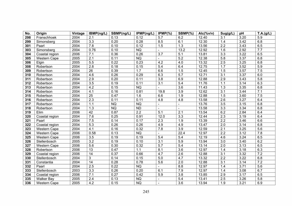
245

No. Origin Vintage IBMP(ng/L) SBMP(ng/L) IPMP(ng/L) IPMP(%) SBMP(%) Alc(%v/v) Sug(g/L) pH T.A.(g/L) 298 Franschhoek 2004 2.1 0.13 0.12 5.7 6.2 12.40 3.1 3.20 5.9 299 Simonsberg 2004 3.3 0.20 0.28 8.5 6.1 12.30 1.4 3.42 6.8 301 Paarl 2004 7.8 0.10 0.12 1.5 1.3 13.56 2.2 3.43 6.5 303 Simonsberg 2004 0.76 0.10 NQ - 13.2 12.92 1.6 2.92 7.7 304 Coastal region 2006 7.1 0.36 0.26 3.7 5.1 13.81 3.3 3.22 6.5 305 Western Cape 2005 2.1 0.11 NQ - 5.2 12.38 5.8 3.37 6.8 306 Elgin 2005 5.5 0.22 0.23 4.2 4.0 13.32 2.5 3.25 6.8 308 Robertson 2004 2.8 0.18 0.15 5.4 6.4 12.75 1.7 3.52 5.9 309 Robertson 2004 26 0.39 1.7 6.6 1.5 12.45 1.5 3.57 7.5 310 Robertson 2004 4.6 0.26 0.29 6.3 5.7 12.71 3.1 3.37 6.0 311 Robertson 2004 2.9 0.20 0.11 3.8 6.9 12.88 2.9 3.43 5.8 312 Robertson 2004 3.5 0.19 0.11 3.1 5.4 11.76 1.1 3.14 6.3 313 Robertson 2004 4.2 0.15 NQ - 3.6 11.43 1.3 3.35 6.8 314 Robertson 2004 4.1 0.16 0.81 19.8 3.9 12.62 3.1 3.44 7.1 315 Robertson 2004 25 0.47 1.6 6.6 1.9 12.88 1.5 3.60 7.5 316 Robertson 2004 2.3 0.11 0.11 4.8 4.8 13.58 2.6 3.27 6.4 317 Robertson 2004 1.1 NQ NQ - - 13.76 3.5 3.15 6.8 318 Robertson 2004 1.3 NQ ND - - 13.58 3.3 3.34 6.8 319 Elim 2006 42 0.87 2.2 5.1 2.1 13.54 6.2 2.84 6.4 320 Coastal region 2004 7.6 0.25 0.91 12.0 3.3 12.44 2.3 3.19 6.4 321 Paarl 2004 7.5 0.14 0.17 2.3 1.9 13.39 2.2 3.46 6.6 322 Coastal region 2004 5.3 0.26 0.26 4.9 4.9 13.47 2.0 3.14 6.8 323 Western Cape 2004 4.1 0.16 0.32 7.8 3.9 12.59 2.1 3.25 5.6 324 Western Cape 2006 0.58 0.13 NQ - 22.4 12.97 2.2 3.12 7.8 325 Western Cape 2006 3.5 0.19 0.19 5.4 5.4 12.19 4.6 3.24 6.5 326 Stellenbosch 2005 3.2 0.19 0.10 3.1 5.9 13.94 3.0 3.40 6.2 327 Western Cape 2006 5.6 0.30 0.32 5.7 5.4 13.14 2.0 3.13 6.5 328 Robertson 2006 13 0.47 1.1 8.1 3.6 12.97 1.4 3.18 6.3 329 Coastal region 2006 14 0.37 0.66 4.7 2.6 12.88 3.1 3.32 7.2 330 Stellenbosch 2004 3 0.14 0.15 5.0 4.7 13.32 2.2 3.22 6.8 331 Constantia 2004 14 0.28 0.78 5.6 2.0 12.88 3.1 3.14 7.2 332 Paarl 2004 2.5 0.22 NQ - 8.8 12.97 1.4 3.71 5.6 333 Stellenbosch 2003 3.3 0.26 0.20 6.1 7.9 12.97 1.4 3.08 6.7 334 Coastal region 2006 7.1 0.27 0.42 5.9 3.8 13.85 2.9 3.17 6.5 335 Walker Bay 2005 2.4 0.13 NQ - 5.4 13.41 2.5 3.26 5.8 336 Western Cape 2005 4.2 0.15 NQ - 3.6 13.94 1.9 3.21 6.9

246

No. Origin Vintage IBMP(ng/L) SBMP(ng/L) IPMP(ng/L) IPMP(%) SBMP(%) Alc(%v/v) Sug(g/L) pH T.A.(g/L) 337 Western Cape 2005 2.5 0.18 NQ - 7.2 13.14 1.3 3.03 6.5 338 Western Cape 2005 1.8 0.13 0.11 6.1 7.2 12.62 2.6 3.51 6.0 339 Western Cape 2005 1.9 0.17 NQ - 8.9 11.76 2.2 3.29 6.5 340 Western Cape 2005 1.8 0.14 NQ - 7.8 13.41 4.1 3.19 6.6 341 Western Cape 2005 1.2 0.14 NQ - 11.7 13.23 1.4 3.22 6.0 342 Western Cape 2005 4 0.21 0.16 4.0 5.3 12.62 1.7 3.36 6.2 343 Stellenbosch 2005 6.9 0.22 0.19 2.8 3.2 12.88 2.7 3.27 5.6 344 Western Cape 2005 2 0.15 NQ - 7.5 12.88 3.2 3.50 5.5 345 Stellenbosch 2005 4.3 0.16 0.16 3.7 3.7 13.58 2.8 3.29 6.0 346 Western Cape 2005 2.6 0.19 0.19 7.3 7.3 11.76 1.8 3.29 6.8 347 Western Cape 2005 3.6 0.20 0.10 2.8 5.6 12.28 3.2 3.57 5.7 348 Stellenbosch 2005 6.8 0.14 0.37 5.4 2.1 12.36 4.7 3.23 7.9 349 Western Cape 2005 2.2 0.17 NQ - 7.7 11.56 3.4 3.26 6.4 350 Stellenbosch 2004 7.2 0.16 0.11 1.5 2.2 11.68 3.2 3.44 5.5 351 Western Cape 2005 2.9 0.13 0.22 7.6 4.5 11.93 2.4 3.47 6.1 352 Stellenbosch 2005 4.9 0.17 0.24 4.9 3.5 13.58 2.5 3.40 6.4 353 Western Cape 2004 9.1 0.23 0.30 3.3 2.5 12.17 2.0 3.55 5.9 354 Swartland 2005 3.9 0.20 NQ - 5.1 13.49 1.6 3.61 6.4 355 Durbanville 2005 8.5 0.19 0.39 4.6 2.2 12.80 1.9 3.43 6.7 356 Western Cape 2005 5.1 0.10 0.17 3.3 2.0 13.41 2.1 3.68 5.8 357 Coastal region 2005 1.3 0.11 NQ - 8.5 12.97 1.3 3.50 5.8 358 Western Cape 2005 4.5 0.13 0.24 5.3 2.9 13.06 2.4 3.19 6.9 359 Western Cape 2005 3.1 0.76 0.36 11.6 24.5 11.68 2.4 3.45 6.8 360 Elim 2005 14 0.48 1.2 8.5 3.4 13.06 2.0 3.26 6.5 361 Coastal region 2005 3.1 0.17 NQ - 5.5 12.02 1.8 3.21 6.7 362 Western Cape 2005 5.9 0.20 0.41 6.9 3.4 11.68 4.6 3.17 7.0 363 Western Cape 2005 3.1 0.20 ND - 6.5 12.45 2.2 3.27 7.2 364 Western Cape 2005 1.1 0.14 NQ - 12.7 12.97 1.7 3.31 7.4 365 Western Cape 2005 2.6 0.19 ND - 7.3 11.68 2.2 3.36 6.6 366 Western Cape 2005 1.9 0.14 NQ - 7.4 13.85 5.3 3.45 6.5 367 Western Cape 2005 2.3 0.15 NQ - 6.5 12.19 3.1 3.26 6.1 368 Western Cape 2005 1.3 0.18 ND - 13.8 13.17 3.2 3.41 7.3 369 Western Cape 2005 1.1 0.17 NQ - 15.5 12.28 6.3 3.24 6.8 370 Western Cape 2005 2.6 0.15 0.13 5.0 5.8 12.28 2.3 3.44 6.6 371 Stellenbosch 2005 4.6 0.37 0.22 4.8 8.0 12.28 2.3 3.41 6.2 372 Western Cape 2005 1.9 0.15 NQ - 7.9 12.71 3.2 3.50 6.7

247

No. Origin Vintage IBMP(ng/L) SBMP(ng/L) IPMP(ng/L) IPMP(%) SBMP(%) Alc(%v/v) Sug(g/L) pH T.A.(g/L) 373 Wellington 2005 1.4 0.18 NQ - 12.9 12.10 2.9 3.30 6.1 374 Paarl 2005 6 0.23 0.21 3.5 3.8 13.58 1.6 3.32 7.4 375 Western Cape 2005 1.1 0.16 NQ - 14.5 12.88 1.3 3.22 5.2 376 Western Cape 2005 1.6 0.16 ND - 10.0 12.36 1.3 3.44 5.3 377 Paarl 2004 4.4 0.24 0.29 6.6 5.5 13.49 2.2 3.22 6.3 378 Western Cape 2005 3.9 0.21 NQ - 5.4 11.76 3.7 3.26 6.2 379 Western Cape 2005 2.3 0.17 NQ - 7.4 12.02 4.5 3.22 6.2 380 Western Cape 2005 0.98 0.16 ND - 16.3 12.10 4.0 3.44 6.3 381 Western Cape 2005 0.94 0.31 NQ - 33.0 12.36 1.2 3.25 6.5 382 Western Cape 2005 1.8 0.22 NQ - 12.2 12.36 1.4 3.11 6.5 383 Stellenbosch 2004 3.1 0.21 0.18 5.8 6.8 12.97 2.5 3.26 6.4 384 Western Cape 2005 2.2 0.16 NQ - 7.3 14.47 4.8 3.64 5.1 385 Western Cape 2005 2 0.18 ND - 9.0 11.85 4.4 3.17 6.2 386 Western Cape 2005 1.8 0.15 ND - 8.3 11.51 4.2 3.31 7.0 387 Western Cape 2005 4.4 0.19 0.18 4.1 4.3 12.88 2.0 3.48 6.8 388 Western Cape 2005 3.4 0.14 NQ - 4.1 12.71 6.2 3.40 7.4 389 Western Cape 2005 6.1 0.18 0.10 1.6 3.0 12.02 4.0 3.28 7.1 391 Coastal region 2004 5.3 0.22 0.35 6.6 4.2 12.62 2.3 3.33 5.9 393 Coastal region 2003 22 0.27 0.20 0.9 1.2 13.23 1.9 3.35 5.9 394 Western Cape 2005 2.8 0.23 0.19 6.8 8.2 11.85 1.2 3.43 6.5 395 Western Cape 2004 8.6 0.27 0.37 4.3 3.1 12.45 1.6 3.23 6.0 396 Stellenbosch 2004 8.8 0.30 0.46 5.2 3.4 13.88 4.5 3.36 6.3 397 Western Cape 2004 2.8 0.18 0.28 10.0 6.4 12.33 3.3 3.50 5.8 398 Western Cape 2004 4.4 0.20 0.23 5.2 4.5 12.28 6.9 3.46 6.2 399 Paarl 2004 5.7 0.19 0.21 3.7 3.3 13.15 1.2 3.57 7.2 400 Cape Point 2004 13 0.61 0.70 5.4 4.7 13.23 2.5 3.29 6.5 401 Paarl 2004 1.7 0.18 0.13 7.6 10.6 13.24 2.7 3.04 5.8 402 Bottelary 2004 2.3 0.18 0.17 7.4 7.8 13.94 5.6 3.01 7.8 403 Paarl 2004 2.1 0.19 0.12 5.7 9.0 13.14 3.0 2.97 8.9 404 Western Cape 2004 4.7 0.22 0.30 6.4 4.7 11.09 3.6 3.46 5.8 405 Stellenbosch 2004 8.6 0.37 0.78 9.1 4.3 14.29 1.4 3.42 5.6 406 Robertson 2006 4.4 0.17 0.13 3.0 3.9 13.49 3.4 3.20 8.4 407 Stellenbosch 2006 2.8 0.18 ND - 6.4 13.58 3.3 3.42 5.8 408 Coastal region 2005 8.2 0.25 0.40 4.9 3.0 12.88 1.5 3.33 6.4 410 Darling 2005 19 0.61 1.4 7.4 3.2 12.97 1.5 3.40 7.4 411 Simonsberg 2005 3.9 0.44 0.14 3.6 11.3 12.02 1.4 3.26 6.8

248

No. Origin Vintage IBMP(ng/L) SBMP(ng/L) IPMP(ng/L) IPMP(%) SBMP(%) Alc(%v/v) Sug(g/L) pH T.A.(g/L) 412 Paarl 2005 13 0.24 0.33 2.5 1.8 13.06 2.6 3.52 6.6 413 Elgin 2005 9.1 0.32 0.54 5.9 3.5 13.49 1.6 3.24 6.6 414 Constantia 2005 6.5 0.32 0.36 5.5 4.9 12.73 2.8 3.26 6.6 415 Stellenbosch 2005 1 0.11 ND - 11.0 13.41 3.3 3.43 6.0 416 Simonsberg 2005 5.1 0.20 0.12 2.4 3.9 13.32 2.0 3.21 6.6 417 Durbanville 2004 9.6 0.31 0.58 6.0 3.2 12.71 1.5 3.05 7.0 418 Franschhoek 2005 0.9 0.11 NQ - 12.2 12.71 2.0 3.29 6.8 419 Western Cape 2005 4.1 0.20 0.18 4.4 4.9 12.53 2.9 3.26 6.5 420 Western Cape 2005 2.8 0.21 ND - 7.5 11.26 2.8 3.19 6.5 421 Western Cape 2005 2.1 0.17 0.34 16.2 8.1 12.45 2.4 3.43 5.9 422 Coastal region 2005 4.2 0.24 0.21 5.0 5.7 14.11 4.1 3.29 6.6 423 Franschhoek 2005 1.1 NQ ND - - 12.71 3.0 2.98 7.5 424 Western Cape 2005 2.3 0.19 0.12 5.2 8.3 13.06 1.4 3.45 5.9 425 Cape Agulhas 2005 4.2 0.18 0.23 5.5 4.3 12.62 2.2 3.36 5.8 426 Cape Agulhas 2005 9.6 0.23 0.20 2.1 2.4 14.56 2.4 3.15 6.9 427 Coastal region 2005 3.1 0.18 0.20 6.5 5.8 13.06 4.0 3.04 7.3 428 Coastal region 2005 5.8 0.33 0.39 6.7 5.7 13.14 4.3 3.10 7.0 429 Western Cape 2005 0.72 0.13 ND - 18.1 12.71 3.4 2.90 6.4 430 Durbanville 2005 11 0.41 0.79 7.2 3.7 13.67 1.8 3.47 6.8 431 Cape Agulhas 2005 7.4 0.20 0.38 5.1 2.7 14.56 4.3 3.33 6.5 432 Stellenbosch 2005 3.2 0.18 NQ - 5.6 13.49 4.3 3.45 6.1 433 Stellenbosch 2005 5.8 0.29 0.22 3.8 5.0 12.71 1.6 3.06 7.2 434 Stellenbosch 2005 2.7 0.19 NQ - 7.0 13.32 3.6 3.23 6.6 435 Wellington 2005 1.1 0.11 ND - 10.0 13.06 1.5 3.42 4.8 436 Western Cape 2005 3.5 0.13 0.13 3.7 3.7 12.19 2.0 3.24 6.4 437 Wellington 2005 0.72 0.12 NQ - 16.7 11.93 1.5 3.11 6.3 438 Western Cape 2005 0.62 0.16 ND - 25.8 12.10 4.4 3.50 6.2 440 Western Cape 2005 2.1 0.14 NQ - 6.7 12.97 1.6 3.67 5.5 441 Stellenbosch 2005 4.4 0.19 0.14 3.2 4.3 12.88 1.3 3.25 7.5 442 Elim 2005 11 0.24 0.73 6.6 2.2 14.56 3.6 3.17 7.1 443 Western Cape 2005 0.52 0.14 NQ - 26.9 14.02 3.1 3.60 5.9 444 Stellenbosch 2005 6.3 0.17 0.28 4.4 2.7 13.41 2.8 3.42 6.8 445 Western Cape 2005 2.2 0.20 0.18 8.2 9.1 12.19 2.2 3.38 6.3 446 Darling 2005 14 0.49 0.96 6.9 3.5 12.45 1.7 3.72 5.3 447 Western Cape 2005 0.54 0.12 NQ - 22.2 12.80 2.6 3.58 4.3 448 Stellenbosch 2005 8.2 0.20 0.40 4.9 2.4 14.38 2.0 3.14 7.8

249

No. Origin Vintage IBMP(ng/L) SBMP(ng/L) IPMP(ng/L) IPMP(%) SBMP(%) Alc(%v/v) Sug(g/L) pH T.A.(g/L) 449 Constantia 2005 12 0.73 0.76 6.3 6.1 13.14 1.5 3.17 6.2 450 Coastal region 2005 5.7 0.39 0.32 5.6 6.8 12.88 1.4 3.29 7.1 451 Stellenbosch 2005 1.8 NQ NQ - - 13.85 1.0 3.27 6.0 452 Elim 2005 14 0.30 0.72 5.1 2.1 13.14 2.0 3.37 6.6 453 Stellenbosch 2005 9.1 0.33 0.40 4.4 3.6 12.36 5.2 3.11 8.3 454 Franschhoek 2005 0.96 NQ NQ - - 13.76 1.6 3.33 6.2 455 Western Cape 2005 3.7 0.13 NQ - 3.5 11.51 2.3 3.32 6.9 456 Coastal region 2005 4.2 0.29 0.20 4.8 6.9 12.88 1.2 3.34 7.0 457 Coastal region 2005 16 0.39 0.63 3.9 2.4 13.94 3.6 3.36 7.4 458 Coastal region 2005 5.7 0.33 0.41 7.2 5.8 12.88 4.0 3.20 6.4 459 Elgin 2004 3.6 0.13 0.21 5.8 3.6 12.97 1.7 3.16 7.5 460 Stellenbosch 2005 2.3 NQ NQ - - 12.97 3.3 3.19 7.1 461 Constantia 2005 9 0.56 0.43 4.8 6.2 13.41 2.4 3.30 6.4 462 Western Cape 2004 2.7 0.18 ND - 6.7 12.10 1.3 3.17 6.4 463 Coastal region 2005 4.8 0.17 0.13 2.7 3.5 12.80 1.8 3.31 6.3 464 Western Cape 2005 0.54 NQ NQ - - 12.28 1.6 3.60 5.3 465 Franschhoek 2005 7.8 0.28 0.50 6.4 3.6 13.85 2.5 3.42 6.9 466 Paarl 2005 7.3 0.20 0.28 3.8 2.7 13.06 1.4 3.65 6.4 467 Walker Bay 2005 8.4 0.25 0.30 3.6 3.0 13.06 1.7 3.04 6.8 468 Durbanville 2003 0.74 0.18 NQ - 24.3 12.02 1.7 3.56 5.2 469 Western Cape 2005 2.9 0.15 0.12 4.1 5.2 12.36 3.1 3.27 5.9 470 Stellenbosch 2005 3.9 0.11 0.20 5.1 2.8 14.65 6.7 3.14 6.6 471 Coastal region 2005 7.7 0.29 0.26 3.4 3.8 12.36 4.4 3.10 7.3 472 Western Cape 2005 1.3 0.13 NQ - 10.0 12.62 1.5 3.56 6.4 473 Coastal region 2005 4.6 0.17 0.13 2.8 3.7 12.88 1.5 3.28 6.3 474 Western Cape 2004 1.7 0.13 NQ - 7.6 12.10 1.2 3.26 6.3 475 Stellenbosch 2005 6.1 0.13 0.22 3.6 2.1 13.14 2.1 2.99 6.5 476 Western Cape 2005 0.48 NQ NQ - - 12.97 1.7 3.31 7.4 477 Coastal region 2005 4.4 0.24 0.14 3.2 5.5 13.58 2.6 3.10 7.4 478 Stellenbosch 2005 2 0.14 0.14 7.0 7.0 12.71 2.9 3.46 6.3 479 Constantia 2005 7.3 0.29 0.43 5.9 4.0 12.53 3.8 3.11 7.6 480 Paarl 2004 2.4 0.17 0.16 6.7 7.1 14.38 3.0 3.68 5.2 481 Stellenbosch 2004 11 0.45 1.1 10.0 4.1 12.53 5.0 3.36 6.7 482 Groenekloof 2005 15 0.55 0.98 6.5 3.7 12.80 1.3 3.40 7.1 483 Durbanville 2003 2.9 0.17 0.17 5.9 5.9 12.19 2.3 3.31 5.9 485 Western Cape 2005 7.6 0.25 0.36 4.7 3.3 13.14 2.6 3.16 7.1

250

No. Origin Vintage IBMP(ng/L) SBMP(ng/L) IPMP(ng/L) IPMP(%) SBMP(%) Alc(%v/v) Sug(g/L) pH T.A.(g/L) 487 Stellenbosch 2005 6.7 0.28 0.37 5.5 4.2 14.47 1.5 3.40 6.0 489 Simonsberg 2005 5 0.20 0.17 3.4 4.0 12.97 2.0 3.33 7.0 490 Durbanville 2004 8.7 0.32 0.44 5.1 3.7 13.32 1.8 3.40 6.6 491 Western Cape 2004 2.6 NQ 0.13 5.0 - 13.94 3.6 3.41 6.7 492 Coastal region 2006 17 0.39 0.72 4.2 2.3 13.23 2.8 3.32 6.9 493 Robertson 2006 2.1 ND NQ - - 12.19 2.3 3.28 7.0 494 Stellenbosch 2005 3.3 0.32 0.15 4.5 9.7 14.56 4.0 3.31 6.3 495 Coastal region 2005 1.8 NQ 0.34 18.9 1.7 11.59 2.9 3.27 5.9 496 Coastal region 2004 4.6 NQ 0.22 4.8 - 13.58 1.4 3.25 6.6 497 Coastal region 2004 11 0.26 0.66 6.0 2.4 12.28 1.9 3.44 6.2 498 Western Cape 2004 3.7 NQ NQ - - 11.93 6.2 3.44 6.8 499 Western Cape 2004 7.2 0.13 0.45 6.3 1.8 13.23 3.4 3.31 6.5 500 Western Cape 2005 40 0.78 2.4 5.9 2.0 15.19 2.0 3.54 5.8 501 Elgin 2006 6 0.18 0.41 6.8 3.0 12.80 2.3 3.36 6.7 502 Paarl 2005 0.54 0.26 NQ - 48.1 12.28 1.5 3.69 5.0 503 Western Cape 2005 1.1 NQ NQ - - 13.49 3.5 3.54 6.1 504 Wellington 2005 0.6 ND NQ - - 12.02 1.2 3.25 6.5 505 Stellenbosch 2005 5.4 NQ 0.16 3.0 - 13.76 2.2 3.12 7.4 506 Constantia 2005 12 2.0 1.2 10.2 16.3 13.23 2.1 3.25 7.1 507 Stellenbosch 2005 8.4 0.14 0.48 5.7 1.7 12.10 5.0 3.07 8.0 508 Stellenbosch 2005 7.4 0.22 0.47 6.4 3.0 13.67 1.8 3.42 6.2 509 Western Cape 2004 2.7 NQ 0.14 5.2 - 11.76 1.6 3.25 7.1 510 Stellenbosch 2005 2.6 NQ NQ - - 13.67 2.6 3.17 5.9 511 Constantia 2005 7 0.26 0.36 5.1 3.7 12.97 2.6 3.15 7.5 512 Western Cape 2005 4.3 0.12 0.24 5.6 2.8 12.80 2.9 3.29 6.9 513 Western Cape 2005 3.4 NQ 0.11 3.2 - 12.53 1.6 3.48 6.3 514 Stellenbosch 2004 1.3 ND NQ - - 13.49 6.2 3.62 5.5 515 Western Cape 2004 9.8 0.25 1.1 10.7 2.6 12.02 1.9 3.91 5.3 516 Stellenbosch 2004 8.4 0.23 0.45 5.4 2.7 12.19 4.0 3.43 6.2 517 Elgin 2005 13 0.26 0.88 6.8 2.0 13.06 1.2 3.37 5.6 518 Western Cape 2005 43 1.0 3.3 7.7 2.3 15.19 2.0 3.54 5.8 519 Coastal region 2005 5 0.18 0.20 4.0 3.6 14.11 4.1 3.29 6.6 520 Western Cape 2004 6.7 0.16 0.49 7.3 2.4 12.62 4.1 3.22 5.4 521 Simonsberg 2005 5.2 NQ 0.13 2.5 - 13.14 2.2 3.27 6.8 522 Simonsberg 2005 4.3 0.36 0.14 3.3 8.4 12.02 1.4 3.26 6.8 523 Stellenbosch 2005 3.8 NQ 0.15 3.9 - 13.32 1.9 3.22 6.5

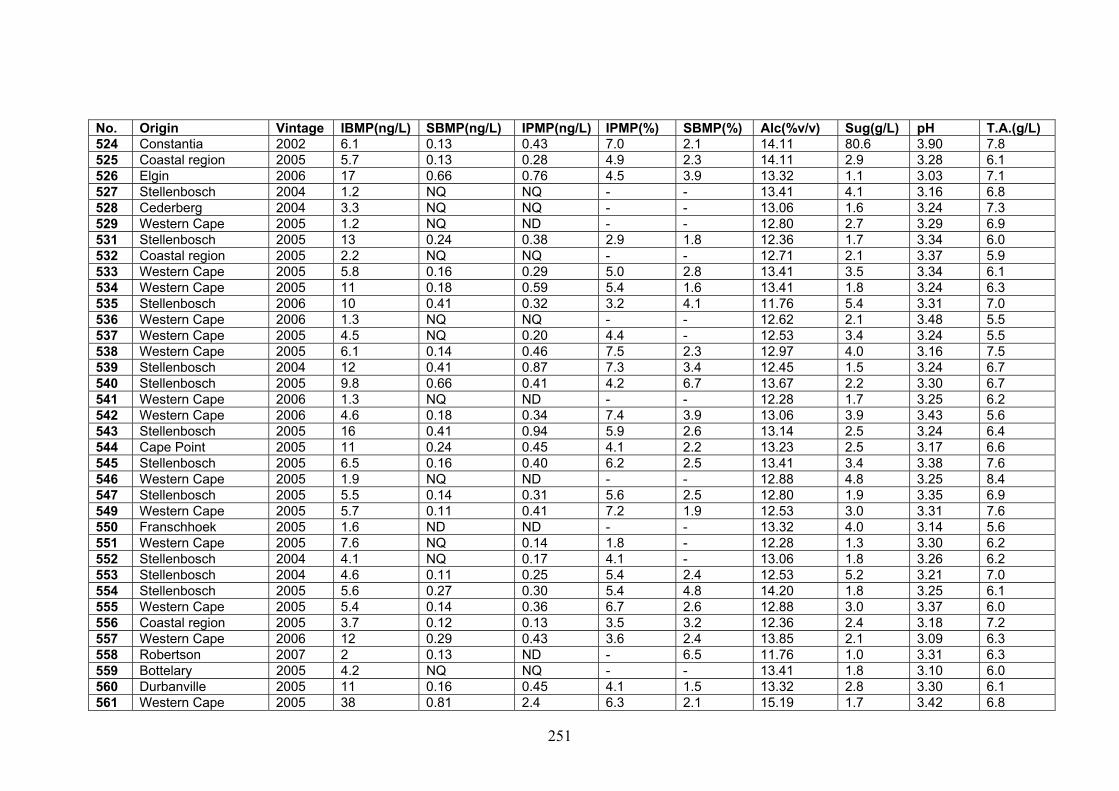
251

No. Origin Vintage IBMP(ng/L) SBMP(ng/L) IPMP(ng/L) IPMP(%) SBMP(%) Alc(%v/v) Sug(g/L) pH T.A.(g/L) 524 Constantia 2002 6.1 0.13 0.43 7.0 2.1 14.11 80.6 3.90 7.8 525 Coastal region 2005 5.7 0.13 0.28 4.9 2.3 14.11 2.9 3.28 6.1 526 Elgin 2006 17 0.66 0.76 4.5 3.9 13.32 1.1 3.03 7.1 527 Stellenbosch 2004 1.2 NQ NQ - - 13.41 4.1 3.16 6.8 528 Cederberg 2004 3.3 NQ NQ - - 13.06 1.6 3.24 7.3 529 Western Cape 2005 1.2 NQ ND - - 12.80 2.7 3.29 6.9 531 Stellenbosch 2005 13 0.24 0.38 2.9 1.8 12.36 1.7 3.34 6.0 532 Coastal region 2005 2.2 NQ NQ - - 12.71 2.1 3.37 5.9 533 Western Cape 2005 5.8 0.16 0.29 5.0 2.8 13.41 3.5 3.34 6.1 534 Western Cape 2005 11 0.18 0.59 5.4 1.6 13.41 1.8 3.24 6.3 535 Stellenbosch 2006 10 0.41 0.32 3.2 4.1 11.76 5.4 3.31 7.0 536 Western Cape 2006 1.3 NQ NQ - - 12.62 2.1 3.48 5.5 537 Western Cape 2005 4.5 NQ 0.20 4.4 - 12.53 3.4 3.24 5.5 538 Western Cape 2005 6.1 0.14 0.46 7.5 2.3 12.97 4.0 3.16 7.5 539 Stellenbosch 2004 12 0.41 0.87 7.3 3.4 12.45 1.5 3.24 6.7 540 Stellenbosch 2005 9.8 0.66 0.41 4.2 6.7 13.67 2.2 3.30 6.7 541 Western Cape 2006 1.3 NQ ND - - 12.28 1.7 3.25 6.2 542 Western Cape 2006 4.6 0.18 0.34 7.4 3.9 13.06 3.9 3.43 5.6 543 Stellenbosch 2005 16 0.41 0.94 5.9 2.6 13.14 2.5 3.24 6.4 544 Cape Point 2005 11 0.24 0.45 4.1 2.2 13.23 2.5 3.17 6.6 545 Stellenbosch 2005 6.5 0.16 0.40 6.2 2.5 13.41 3.4 3.38 7.6 546 Western Cape 2005 1.9 NQ ND - - 12.88 4.8 3.25 8.4 547 Stellenbosch 2005 5.5 0.14 0.31 5.6 2.5 12.80 1.9 3.35 6.9 549 Western Cape 2005 5.7 0.11 0.41 7.2 1.9 12.53 3.0 3.31 7.6 550 Franschhoek 2005 1.6 ND ND - - 13.32 4.0 3.14 5.6 551 Western Cape 2005 7.6 NQ 0.14 1.8 - 12.28 1.3 3.30 6.2 552 Stellenbosch 2004 4.1 NQ 0.17 4.1 - 13.06 1.8 3.26 6.2 553 Stellenbosch 2004 4.6 0.11 0.25 5.4 2.4 12.53 5.2 3.21 7.0 554 Stellenbosch 2005 5.6 0.27 0.30 5.4 4.8 14.20 1.8 3.25 6.1 555 Western Cape 2005 5.4 0.14 0.36 6.7 2.6 12.88 3.0 3.37 6.0 556 Coastal region 2005 3.7 0.12 0.13 3.5 3.2 12.36 2.4 3.18 7.2 557 Western Cape 2006 12 0.29 0.43 3.6 2.4 13.85 2.1 3.09 6.3 558 Robertson 2007 2 0.13 ND - 6.5 11.76 1.0 3.31 6.3 559 Bottelary 2005 4.2 NQ NQ - - 13.41 1.8 3.10 6.0 560 Durbanville 2005 11 0.16 0.45 4.1 1.5 13.32 2.8 3.30 6.1 561 Western Cape 2005 38 0.81 2.4 6.3 2.1 15.19 1.7 3.42 6.8

252

No. Origin Vintage IBMP(ng/L) SBMP(ng/L) IPMP(ng/L) IPMP(%) SBMP(%) Alc(%v/v) Sug(g/L) pH T.A.(g/L) 562 Constantia 2005 13 1.1 1.1 8.7 8.2 13.67 2.6 3.45 6.5 563 Western Cape 2005 10 0.21 0.48 4.8 2.1 13.23 1.1 3.30 6.3 564 Stellenbosch 2005 1.7 NQ ND - - 13.23 2.8 3.34 6.7 565 Stellenbosch 2005 5.5 0.14 0.32 5.8 2.5 13.14 3.3 3.39 7.6 566 Stellenbosch 2005 6 0.11 0.39 6.5 1.8 12.36 6.1 3.35 6.4 567 Western Cape 2004 2.6 NQ 0.17 6.5 - 13.67 5.0 3.44 5.8 568 Coastal region 2005 14 0.38 0.81 5.8 2.7 13.67 2.0 3.22 6.7 569 Western Cape 2007 18 0.42 1.1 6.2 2.3 12.62 1.4 2.96 7.7 570 Western Cape 2005 5.4 NQ 0.21 3.9 - 12.36 4.0 3.28 6.7 571 Durbanville 2005 12 0.20 0.44 3.7 1.7 11.68 1.2 3.40 6.0 572 Franschhoek 2005 1.1 NQ NQ - - 14.65 1.3 3.32 5.9 573 Western Cape 2005 3.6 NQ 0.24 6.7 - 12.62 1.7 3.36 6.2 574 Stellenbosch 2005 8.4 0.21 0.49 5.8 2.5 13.94 2.2 3.26 7.7 576 Simonsberg 2005 5.9 0.12 0.32 5.4 2.0 12.71 1.5 3.30 7.1 577 Stellenbosch 2004 4.2 NQ 0.20 4.8 - 12.53 1.5 3.36 6.4 578 Cape Agulhas 2005 4.9 NQ 0.38 7.8 - 12.62 2.2 3.36 5.8 579 Simonsberg 2005 8.1 0.21 0.55 6.8 2.6 13.76 1.6 3.35 6.3 580 Stellenbosch 2005 3.9 0.11 0.32 8.2 2.8 13.58 1.5 3.40 5.7 581 Cape Agulhas 2005 13 0.23 0.82 6.3 1.8 13.06 2.0 3.26 6.5 582 Coastal region 2005 7.7 NQ 0.20 2.6 - 12.71 3.4 3.42 6.5 583 Elim 2005 9.5 0.28 0.73 7.7 2.9 13.58 2.9 3.28 6.7 584 Walker Bay 2005 1.2 NQ 0.13 10.8 - 13.58 1.6 3.33 6.4 585 Coastal region 2005 3.7 NQ 0.14 3.8 - 12.02 2.3 3.22 6.3 586 Paarl 2005 20 NQ 0.18 0.9 - 13.41 2.3 3.44 6.6 587 Western Cape 2005 5.3 0.11 0.16 3.0 2.1 12.19 3.6 3.31 5.8 588 Stellenbosch 2004 20 0.26 0.65 3.3 1.3 12.45 3.4 3.51 6.5 589 Western Cape 2005 44 0.83 3.9 9.0 1.9 15.19 2.0 3.60 5.9 590 Western Cape 2006 24 0.67 2.1 8.7 2.8 12.80 3.4 3.27 6.6 593 Coastal region 2005 4.1 NQ NQ - - 12.10 2.6 3.22 6.0 594 Simonsberg 2005 4.9 0.11 0.16 3.3 2.2 13.58 2.5 3.40 6.4 595 Constantia 2005 9.1 0.51 0.40 4.4 5.6 13.06 2.6 3.30 2.6 596 Paarl 2005 0.78 NQ NQ - - 13.06 2.8 3.44 5.4 597 Coastal region 2005 2.9 NQ NQ - - 12.88 4.7 2.97 6.8 598 Bottelary 2005 7 0.26 0.45 6.4 3.7 13.76 2.7 3.21 6.8 599 Western Cape 2006 23 0.51 1.5 6.3 2.2 12.8 3.7 3.28 6.7 600 Robertson 2007 5.7 0.12 0.32 5.6 2.1 12.42 0.7 3.60 8.1

253

No. Origin Vintage IBMP(ng/L) SBMP(ng/L) IPMP(ng/L) IPMP(%) SBMP(%) Alc(%v/v) Sug(g/L) pH T.A.(g/L) 601 Durbanville 1999 16 0.43 1.8 11.4 2.7 12.93 2.0 3.53 7.4 602 Durbanville 2000 6.4 NQ 0.26 4.1 - 12.98 2.5 3.45 6.5 603 Durbanville 2001 38 0.69 2.5 6.6 1.8 13.00 2.8 3.22 7.5 604 Durbanville 2002 20 0.60 2.2 10.8 3.0 12.76 1.8 3.32 7.7 605 Durbanville 2003 14 0.35 1.5 11.0 2.5 12.57 1.8 3.42 7.2

a = adulterated sample 1

b = adulterated sample 2

ND = not detected

NQ = not quantified

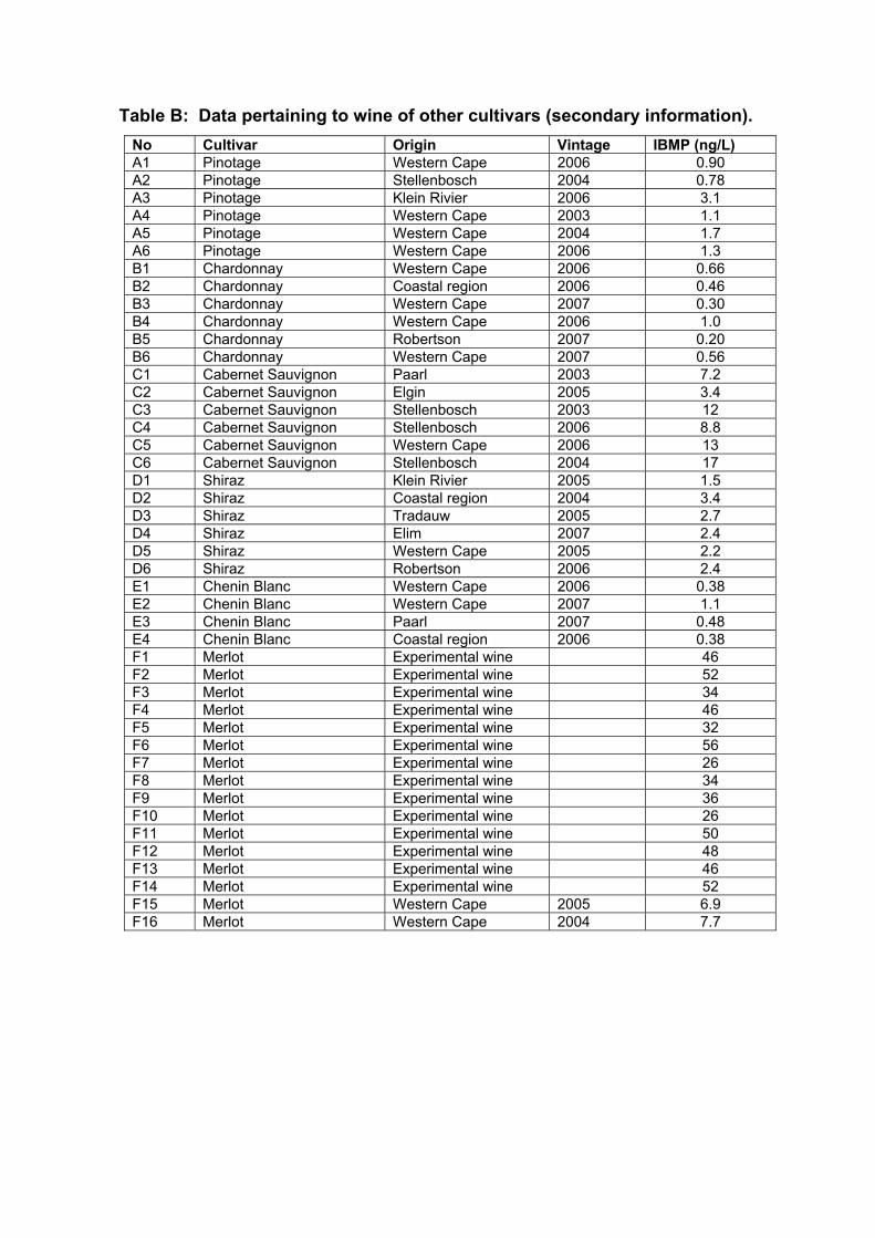
Table B: Data pertaining to wine of other cultivars (secondary information). No Cultivar Origin Vintage IBMP (ng/L) A1 Pinotage Western Cape 2006 0.90 A2 Pinotage Stellenbosch 2004 0.78 A3 Pinotage Klein Rivier 2006 3.1 A4 Pinotage Western Cape 2003 1.1 A5 Pinotage Western Cape 2004 1.7 A6 Pinotage Western Cape 2006 1.3 B1 Chardonnay Western Cape 2006 0.66 B2 Chardonnay Coastal region 2006 0.46 B3 Chardonnay Western Cape 2007 0.30 B4 Chardonnay Western Cape 2006 1.0 B5 Chardonnay Robertson 2007 0.20 B6 Chardonnay Western Cape 2007 0.56 C1 Cabernet Sauvignon Paarl 2003 7.2 C2 Cabernet Sauvignon Elgin 2005 3.4 C3 Cabernet Sauvignon Stellenbosch 2003 12 C4 Cabernet Sauvignon Stellenbosch 2006 8.8 C5 Cabernet Sauvignon Western Cape 2006 13 C6 Cabernet Sauvignon Stellenbosch 2004 17 D1 Shiraz Klein Rivier 2005 1.5 D2 Shiraz Coastal region 2004 3.4 D3 Shiraz Tradauw 2005 2.7 D4 Shiraz Elim 2007 2.4 D5 Shiraz Western Cape 2005 2.2 D6 Shiraz Robertson 2006 2.4 E1 Chenin Blanc Western Cape 2006 0.38 E2 Chenin Blanc Western Cape 2007 1.1 E3 Chenin Blanc Paarl 2007 0.48 E4 Chenin Blanc Coastal region 2006 0.38 F1 Merlot Experimental wine 46 F2 Merlot Experimental wine 52 F3 Merlot Experimental wine 34 F4 Merlot Experimental wine 46 F5 Merlot Experimental wine 32 F6 Merlot Experimental wine 56 F7 Merlot Experimental wine 26 F8 Merlot Experimental wine 34 F9 Merlot Experimental wine 36 F10 Merlot Experimental wine 26 F11 Merlot Experimental wine 50 F12 Merlot Experimental wine 48 F13 Merlot Experimental wine 46 F14 Merlot Experimental wine 52 F15 Merlot Western Cape 2005 6.9 F16 Merlot Western Cape 2004 7.7

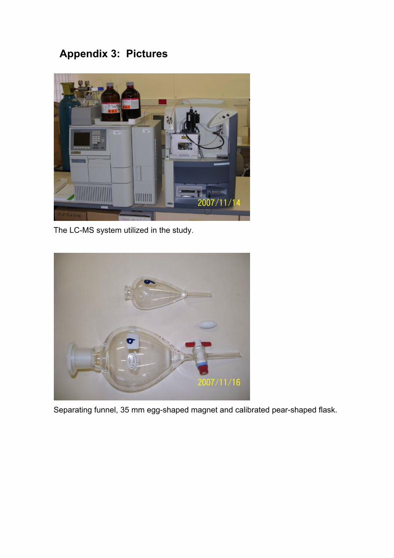
Appendix 3: Pictures

The LC-MS system utilized in the study.

Separating funnel, 35 mm egg-shaped magnet and calibrated pear-shaped flask.

256

Distillation apparatus with 60 cm fractionating column.

Equipment for evaporation of solvent from sample extracts.

development of a novel lc-ms/ms method …development of a novel lc-ms/ms method for the detection...

Documents