development of a novel hvdc system model for control design
TRANSCRIPT
This article was downloaded by: [American Public University System]On: 03 May 2013, At: 07:42Publisher: Taylor & FrancisInforma Ltd Registered in England and Wales Registered Number:1072954 Registered office: Mortimer House, 37-41 Mortimer Street,London W1T 3JH, UK
Electric Machines & PowerSystemsPublication details, including instructions forauthors and subscription information:http://www.tandfonline.com/loi/uemp19
Development of a NovelHVDC System Model forControl DesignR. K. Pandey, Arindam Ghosh, SachchidanandPublished online: 29 Oct 2010.
To cite this article: R. K. Pandey, Arindam Ghosh, Sachchidanand (1999):Development of a Novel HVDC System Model for Control Design, Electric Machines& Power Systems, 27:11, 1243-1257
To link to this article: http://dx.doi.org/10.1080/073135699268696
PLEASE SCROLL DOWN FOR ARTICLE
Full terms and conditions of use: http://www.tandfonline.com/page/terms-and-conditions
This article may be used for research, teaching, and private studypurposes. Any substantial or systematic reproduction, redistribution,reselling, loan, sub-licensing, systematic supply, or distribution in anyform to anyone is expressly forbidden.
The publisher does not give any warranty express or implied or makeany representation that the contents will be complete or accurate orup to date. The accuracy of any instructions, formulae, and drug dosesshould be independently verified with primary sources. The publishershall not be liable for any loss, actions, claims, proceedings, demand, orcosts or damages whatsoever or howsoever caused arising directly orindirectly in connection with or arising out of the use of this material.
Electric Machines and Power Systems, 27:1243–1257, 1999Copyright c° 1999 Taylor & Francis, Inc.0731-356X / 99 $12.00 + .00
Development of a Novel HVDC System Modelfor Control Design
R. K. PANDEY
Department of Electrical EngineeringInstitute of TechnologyBanaras Hindu UniversityVaranasi-221 005, India
ARINDAM GHOSHSACHCHIDANAND
Department of Electrical EngineeringIndian Institute of TechnologyKanpur-208 016, India
The operation of HVDC converters is discrete in nature. It is, therefore, properto take into account the discrete behavior of converter operation while devel-oping the system model for small signal stability analysis. This paper presentsthe development of such a system model, which also explicitly includes the ef-fect of phase angle of respective AC bus voltages. A modular approach has beenadopted for the formulation of complete state space system model. Utilizing thesystem model, the stability is examined in the controller parameter plane usingeigenvalue analysis. The stability domains thus obtained are validated throughdetailed dynamic digital simulation.
Keywords HVDC, multirate sampling, discrete-time, continuous-time, IPC
1 Introduction
The study of low frequency oscillations in an integrated AC/ DC power systemand the control design for damping these oscillations based on small signal stabil-ity analysis has become vital for modern power systems. An improperly designedcontroller would degrade the system performance by aggravating adverse dynamicinteractions. An HVDC system is a large scale multivariable system that is bothnonlinear and prone to external disturbances. This makes the stability investiga-tions extremely complex. A standard practice to overcome this problem is to carryout stability investigations using linearized perturbation models in which the sys-tem is linearized around a nominal operating point. Although representation ofpower system in linear domain is adequate for small signal stability analysis, it isessential that the extent of details included in system representation should enablestudy of both local and global eŒects of the controls. To achieve this objective, it is
Manuscript received in �nal form on January 4, 1999.Address correspondence to R. K. Pandey.
1243
Dow
nloa
ded
by [
Am
eric
an P
ublic
Uni
vers
ity S
yste
m]
at 0
7:42
03
May
201
3
1244 R. K. Pandey et al.
important that the behavior of various components of the HVDC system be appro-priately represented in a linear domain. In this context, both continuous-time anddiscrete-time system representation have been described in the literature [1–12]. Inthe development of continuous-time system model, the converter is represented asa voltage source described by the average DC voltage equation of the converter.In discrete-time representation, the converter is modeled, taking into considerationthe discrete nature of its control that is eŒective not only at discrete-time instantscorresponding to the valve �ring instants, but also at the instants correspondingto the completion of the commutation process. Both of these discrete-time instantsneed to be adequately taken into consideration while representing the converter forsmall signal stability investigations [11]. Although the stability analysis reported in[11] and other publications consider that the AC voltages on the two ends of theDC line are synchronized, the practical situation may not be quite so.
The paper describes the development of a two-terminal HVDC system modelin a state space framework. In the recti�er and inverter operation, the beginning ofa valve conduction and the end of commutation process are not assumed coincidentin general. In steady state this leads to four discrete-time instants in an interval of60° . The DC link model in such a situation has been derived employing the theoryof multirate sampling [11]. Although the DC link model presented in this paperignores the detailed representation of AC system under the assumption that thehost AC systems at the two ends are strong, it explicitly represents the phase angleseparation of the converter AC bus voltages. The system model is used for stabilityanalysis of a two-terminal sample system. The stability domains are obtained inthe controller parameter plane using eigenvalue analysis. The stability regions arefurther validated through detailed digital simulation. The eŒects of variation in (a)the AC bus voltage phase angle separation, (b) the inverter extinction angle ° , and(c) transformer leakage reactance has been examined on converter control stability.
2 System Model
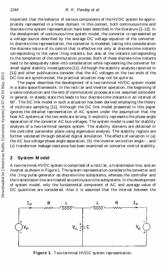
A two-terminal HVDC system is comprised of a recti�er, a transmission line, and aninverter as shown in Figure 1. The system representation considers the converter andthe �ring pulse generator as discrete-time subsystems, whereas the controller andthe transmission line are treated as continuous-time subsystems. In the developmentof system model, only the fundamental component of AC and average value ofDC quantities are considered. Also it is assumed that the interval between the
Figure 1. Two-terminal HVDC system representation.
Dow
nloa
ded
by [
Am
eric
an P
ublic
Uni
vers
ity S
yste
m]
at 0
7:42
03
May
201
3
Development of a Novel HVDC System Model 1245
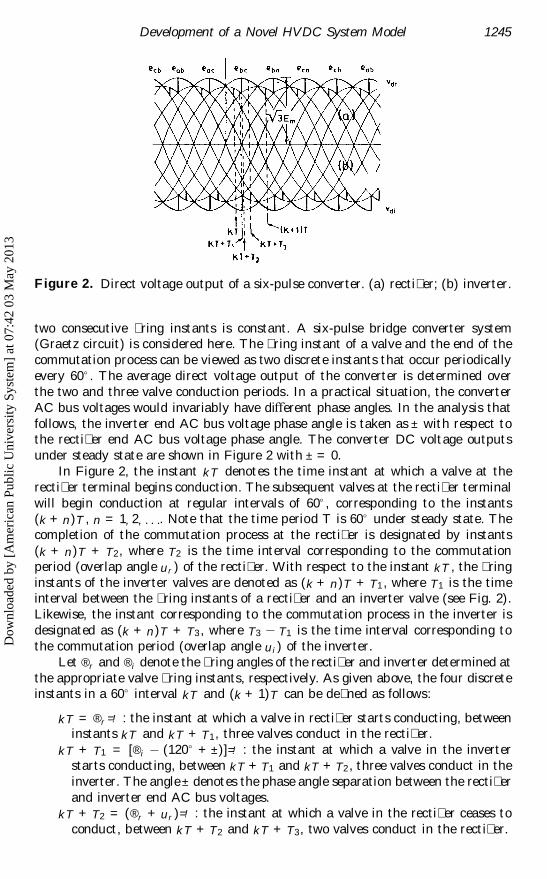
Figure 2. Direct voltage output of a six-pulse converter. (a) recti�er; (b) inverter.
two consecutive �ring instants is constant. A six-pulse bridge converter system(Graetz circuit) is considered here. The �ring instant of a valve and the end of thecommutation process can be viewed as two discrete instants that occur periodicallyevery 60° . The average direct voltage output of the converter is determined overthe two and three valve conduction periods. In a practical situation, the converterAC bus voltages would invariably have diŒerent phase angles. In the analysis thatfollows, the inverter end AC bus voltage phase angle is taken as ± with respect tothe recti�er end AC bus voltage phase angle. The converter DC voltage outputsunder steady state are shown in Figure 2 with ± = 0.
In Figure 2, the instant kT denotes the time instant at which a valve at therecti�er terminal begins conduction. The subsequent valves at the recti�er terminalwill begin conduction at regular intervals of 60° , corresponding to the instants(k + n)T , n = 1, 2, . . .. Note that the time period T is 60° under steady state. Thecompletion of the commutation process at the recti�er is designated by instants(k + n)T + T2, where T2 is the time interval corresponding to the commutationperiod (overlap angle ur ) of the recti�er. With respect to the instant kT , the �ringinstants of the inverter valves are denoted as (k + n)T + T1, where T1 is the timeinterval between the �ring instants of a recti�er and an inverter valve (see Fig. 2).Likewise, the instant corresponding to the commutation process in the inverter isdesignated as (k + n)T + T3, where T3 T1 is the time interval corresponding tothe commutation period (overlap angle ui) of the inverter.
Let ®r and ®i denote the �ring angles of the recti�er and inverter determined atthe appropriate valve �ring instants, respectively. As given above, the four discreteinstants in a 60° interval kT and (k + 1)T can be de�ned as follows:
kT = ®r =!: the instant at which a valve in recti�er starts conducting, betweeninstants kT and kT + T1, three valves conduct in the recti�er.
kT + T1 = [®i (120° + ±)]=!: the instant at which a valve in the inverterstarts conducting, between kT + T1 and kT + T2, three valves conduct in theinverter. The angle± denotes the phase angle separation between the recti�erand inverter end AC bus voltages.
kT + T2 = (®r + ur )=!: the instant at which a valve in the recti�er ceases toconduct, between kT + T2 and kT + T3, two valves conduct in the recti�er.
Dow
nloa
ded
by [
Am
eric
an P
ublic
Uni
vers
ity S
yste
m]
at 0
7:42
03
May
201
3
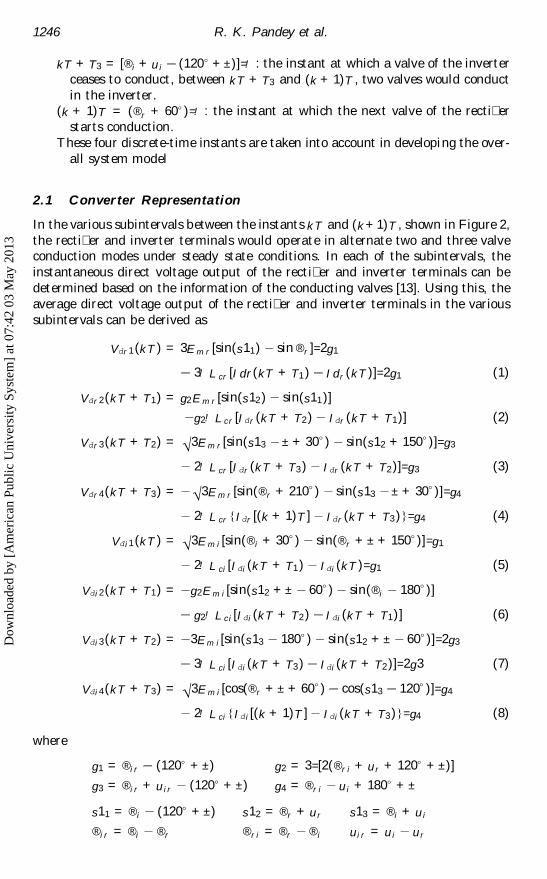
1246 R. K. Pandey et al.
kT + T3 = [®i + ui (120° + ±)]=!: the instant at which a valve of the inverterceases to conduct, between kT + T3 and (k + 1)T , two valves would conductin the inverter.
(k + 1)T = (®r + 60° )=!: the instant at which the next valve of the recti�erstarts conduction.
These four discrete-time instants are taken into account in developing the over-all system model
2.1 Converter Representation
In the various subintervals between the instants kT and (k + 1)T , shown in Figure 2,the recti�er and inverter terminals would operate in alternate two and three valveconduction modes under steady state conditions. In each of the subintervals, theinstantaneous direct voltage output of the recti�er and inverter terminals can bedetermined based on the information of the conducting valves [13]. Using this, theaverage direct voltage output of the recti�er and inverter terminals in the varioussubintervals can be derived as
Vdr 1(kT ) = 3E m r [sin(s11) sin®r ]=2g1
3!L cr [I dr(kT + T1) I dr (kT )]=2g1 (1)
Vdr 2(kT + T1) = g2E m r [sin(s12) sin(s11)]
g2!L cr [Idr (kT + T2) Idr (kT + T1)] (2)
Vdr 3(kT + T2) = Ö 3E m r [sin(s13 ± + 30° ) sin(s12 + 150° )]=g3
2!L cr [I dr (kT + T3) Idr (kT + T2)]=g3 (3)
Vdr 4(kT + T3) = Ö 3E m r [sin(®r + 210° ) sin(s13 ± + 30° )]=g4
2!L cr {Idr [(k + 1)T ] Idr (kT + T3)}=g4 (4)
Vdi1(kT ) = Ö 3E m i[sin(®i + 30° ) sin(®r + ± + 150° )]=g1
2!L ci [Idi(kT + T1) Idi(kT )=g1 (5)
Vdi2(kT + T1) = g2E m i[sin(s12 + ± 60° ) sin(®i 180° )]
g2!L c i[Idi(kT + T2) I di(kT + T1)] (6)
Vdi3(kT + T2) = 3E m i[sin(s13 180° ) sin(s12 + ± 60° )]=2g3
3!L ci [Idi(kT + T3) Idi(kT + T2)]=2g3 (7)
Vdi4(kT + T3) = Ö 3E m i[cos(®r + ± + 60° ) cos(s13 120° )]=g4
2!L ci{Idi[(k + 1)T ] Idi(kT + T3)}=g4 (8)
where
g1 = ®ir (120° + ±) g2 = 3=[2(®r i + ur + 120° + ±)]
g3 = ®ir + uir (120° + ±) g4 = ®r i ui + 180° + ±
s11 = ®i (120° + ±) s12 = ®r + ur s13 = ®i + ui
®ir = ®i ®r ®r i = ®r ®i uir = ui ur
Dow
nloa
ded
by [
Am
eric
an P
ublic
Uni
vers
ity S
yste
m]
at 0
7:42
03
May
201
3
Development of a Novel HVDC System Model 1247
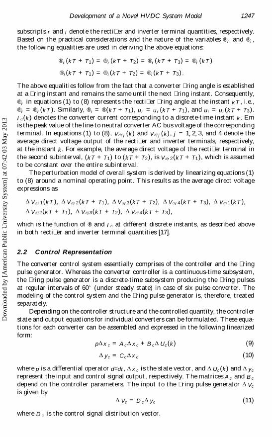
subscripts r and i denote the recti�er and inverter terminal quantities, respectively.Based on the practical considerations and the nature of the variables ®r and ®i ,the following equalities are used in deriving the above equations:
®r (kT + T1) = ®r (kT + T2) = ®r (kT + T3) = ®r (kT )
®i(kT + T1) = ®i(kT + T2) = ®i(kT + T3) .
The above equalities follow from the fact that a converter �ring angle is establishedat a �ring instant and remains the same until the next �ring instant. Consequently,®r in equations (1) to (8) represents the recti�er �ring angle at the instant kT , i.e.,®r = ®r (kT ). Similarly, ®i = ®(kT + T1), ur = ur (kT + T1), and ui = ui(kT + T3).Id (k ) denotes the converter current corresponding to a discrete-time instant k . Emis the peak value of the line to neutral converter AC bus voltage of the correspondingterminal. In equations (1) to (8), Vdr j (k ) and Vdij (k), j = 1, 2, 3, and 4 denote theaverage direct voltage output of the recti�er and inverter terminals, respectively,at the instant k . For example, the average direct voltage of the recti�er terminal inthe second subinterval, (kT + T1) to (kT + T2), is Vdr 2(kT + T1), which is assumedto be constant over the entire subinterval.
The perturbation model of overall system is derived by linearizing equations (1)to (8) around a nominal operating point. This results as the average direct voltageexpressions as
D Vdr 1(kT ), D Vdr 2(kT + T1), D Vdr 3(kT + T2) , D Vdr 4(kT + T3), D Vdi1(kT ),
D Vdi2(kT + T1), D Vdi3(kT + T2), D Vdi4(kT + T3),
which is the function of ® and I d at diŒerent discrete instants, as described abovein both recti�er and inverter terminal quantities [17].
2.2 Control Representation
The converter control system essentially comprises of the controller and the �ringpulse generator. Whereas the converter controller is a continuous-time subsystem,the �ring pulse generator is a discrete-time subsystem producing the �ring pulsesat regular intervals of 60° (under steady state) in case of six pulse converter. Themodeling of the control system and the �ring pulse generator is, therefore, treatedseparately.
Depending on the controller structure and the controlled quantity, the controllerstate and output equations for individual converters can be formulated. These equa-tions for each converter can be assembled and expressed in the following linearizedform:
p D x c = A c D x c + B c D Uc (k ) (9)
D yc = C c D x c (10)
where p is a diŒerential operator d=dt, D x c is the state vector, and D Uc (k ) and D yc
represent the input and control signal output, respectively. The matrices A c and B c
depend on the controller parameters. The input to the �ring pulse generator D Vc
is given byD Vc = D c D yc (11)
where D c is the control signal distribution vector.
Dow
nloa
ded
by [
Am
eric
an P
ublic
Uni
vers
ity S
yste
m]
at 0
7:42
03
May
201
3
1248 R. K. Pandey et al.
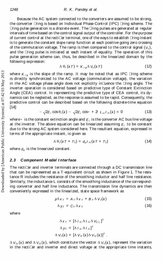
Because the AC system connected to the converters are assumed to be strong,the converter �ring is based on Individual Phase Control (IPC) �ring scheme. The�ring pulse generation is a discrete event. The �ring pulses are generated at regularintervals of time based on the control signal output of the controller. For the purposeof current control at the recti�er terminal, one of the ways to establish �ring instantis to generate the constant slope ramp function at each positive going zero crossingof the commutation voltage. The ramp is then compared to the control signal (Vc ),and the �ring pulse is initiated at each instant of equality. The operation of thispulse generation scheme can, thus, be described in the linearized domain by thefollowing expression:
D ®r (kT ) = K r g D Vc (kT ) (12)
where K r g is the slope of the ramp. It may be noted that as IPC �ring schemeis directly synchronized to the AC voltage (commutation voltage), the variationin the AC voltage phase angle does not explicitly in�uence the �ring angle. Theinverter operation is considered based on predictive type of Constant ExtinctionAngle (CEA) control. In representing the predictive type of CEA control, its dy-namics can be neglected, as the response is assumed to be rapid. Consequently, thepredictive control can be described based on the following discrete-time equation[14]:
Ö 2E i cos®i(k ) Ö 2E i cos° + 2!L c iIdi(k) = 0 (13)
where° is the constant extinction angle and E i is the converter AC bus line voltageat the inverter. The above equation can be linearized assuming E i to be constantdue to the strong AC system considered here. The resultant equation, expressed interms of the appropriate instant, is given as
D ®i(kT + T1) = da I di(kT + T1) (14)
where da is the linearized constant.
2.3 Component Model Interface
The recti�er and inverter terminals are connected through a DC transmission linethat can be represented as a T-equivalent circuit as shown in Figure 1. The resis-tance R includes the resistance of the smoothing inductor and half line resistance.Similarly, the inductance L consists of the smoothing inductance of the correspond-ing converter and half line inductance. The transmission line dynamics are thenconveniently expressed in the linearized, state space framework as
p D x T = A T D x T + B T D Vd(k ) (15)
D yT = CT D x T (16)
where
D x T = [D Idr D Idi D VC L ]T
D yT = [D Idr D Idi]T
D Vd(k ) = [D Vdr (k ) D Vdi(k )]T .
D Vdr (k ) and D Vdi(k ), which constitute the vector D Vd(k ), represent the variationin the recti�er and inverter end direct voltage at the appropriate time instants,
Dow
nloa
ded
by [
Am
eric
an P
ublic
Uni
vers
ity S
yste
m]
at 0
7:42
03
May
201
3
Development of a Novel HVDC System Model 1249
respectively [17]. The matrices A T , B T , and C T can be formed appropriately usingthe line parameters. It will be evident that both the transmission line and con-trol system dynamic equations are continuous in time. These are then combinedtogether as
p D x = A D x + B D Vd (k ) (17)
where A is the state matrix, B T is the input distribution matrix, and
D x = [D x c D Idr D Idi D VC L ]T .
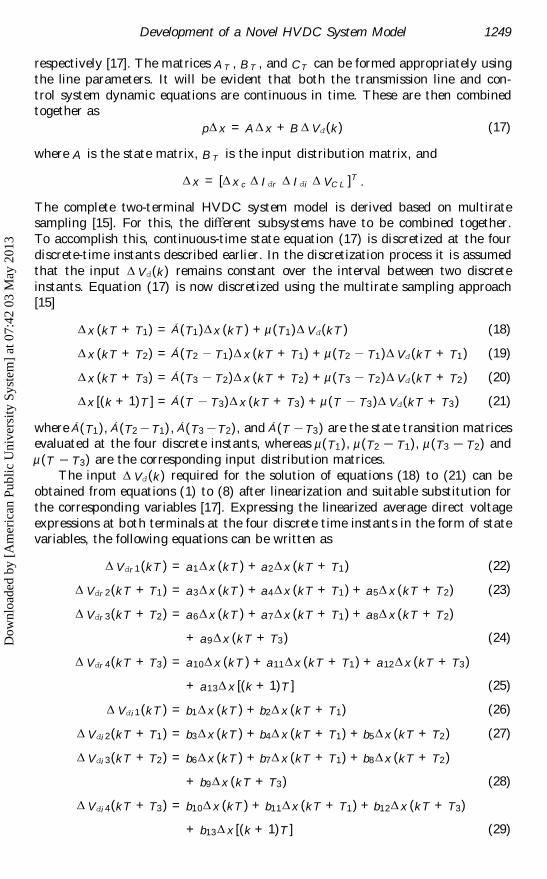
The complete two-terminal HVDC system model is derived based on multiratesampling [15]. For this, the diŒerent subsystems have to be combined together.To accomplish this, continuous-time state equation (17) is discretized at the fourdiscrete-time instants described earlier. In the discretization process it is assumedthat the input D Vd(k ) remains constant over the interval between two discreteinstants. Equation (17) is now discretized using the multirate sampling approach[15]
D x (kT + T1) = Á(T1) D x (kT ) + µ(T1) D Vd(kT ) (18)
D x (kT + T2) = Á(T2 T1) D x (kT + T1) + µ(T2 T1) D Vd (kT + T1) (19)
D x (kT + T3) = Á(T3 T2) D x (kT + T2) + µ(T3 T2) D Vd (kT + T2) (20)
D x [(k + 1)T ] = Á(T T3) D x (kT + T3) + µ(T T3) D Vd(kT + T3) (21)
where Á(T1), Á(T2 T1), Á(T3 T2), and Á(T T3) are the state transition matricesevaluated at the four discrete instants, whereas µ(T1), µ(T2 T1), µ(T3 T2) andµ(T T3) are the corresponding input distribution matrices.
The input D Vd (k ) required for the solution of equations (18) to (21) can beobtained from equations (1) to (8) after linearization and suitable substitution forthe corresponding variables [17]. Expressing the linearized average direct voltageexpressions at both terminals at the four discrete time instants in the form of statevariables, the following equations can be written as
D Vdr 1(kT ) = a1 D x (kT ) + a2 D x (kT + T1) (22)
D Vdr 2(kT + T1) = a3 D x (kT ) + a4 D x (kT + T1) + a5 D x (kT + T2) (23)
D Vdr 3(kT + T2) = a6 D x (kT ) + a7 D x (kT + T1) + a8 D x (kT + T2)
+ a9 D x (kT + T3) (24)
D Vdr 4(kT + T3) = a10 D x (kT ) + a11 D x (kT + T1) + a12 D x (kT + T3)
+ a13 D x [(k + 1)T ] (25)
D Vdi1(kT ) = b1 D x (kT ) + b2 D x (kT + T1) (26)
D Vdi2(kT + T1) = b3 D x (kT ) + b4 D x (kT + T1) + b5 D x (kT + T2) (27)
D Vdi3(kT + T2) = b6 D x (kT ) + b7 D x (kT + T1) + b8 D x (kT + T2)
+ b9 D x (kT + T3) (28)
D Vdi4(kT + T3) = b10 D x (kT ) + b11 D x (kT + T1) + b12 D x (kT + T3)
+ b13 D x [(k + 1)T ] (29)
Dow
nloa
ded
by [
Am
eric
an P
ublic
Uni
vers
ity S
yste
m]
at 0
7:42
03
May
201
3
1250 R. K. Pandey et al.
where a1 to a13 and b1 to b13 are appropriate vectors of dimension 1 ´ 4. Usingequations (22) to (29), the discretized state equations (18) to (21) can be combinedin the following form:
D x [(k + 1)T ] = M D x (kT ) (30)
where M is the closed loop matrix of the system. It is to be noted that the eigenval-ues of matrix M indicate the system stability, i.e., for the stable system operation,the eigenvalues must lie in the unit circle.
3 Case Study
The stability analysis of a two-terminal DC link has been carried out primarily toillustrate the system model developed. The system parameters and operating con-ditions of the sample system are given in the Appendix. The recti�er is consideredto be equipped with the constant current control using �rst order regulator. Thevalve �ring instants are established through IPC �ring scheme. Predictive type ofCEA control is considered at the inverter terminal. Various case studies have beencarried out to investigate the eŒect of variation in the converter AC bus voltagephase angle, extinction angle, and transformer leakage inductance on the stabilitycharacteristics of the system.
EŒect of the Phase Angle
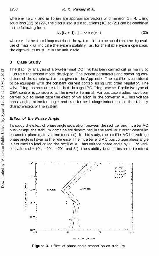
To study the eŒect of phase angle separation between the recti�er and inverter ACbus voltage, the stability domains are determined in the recti�er current controllerparameter plane (gain vs time constant). In this study, the recti�er AC bus voltagephase angle is taken as the reference. The inverter end AC bus voltage phase angleis assumed to lead or lag the recti�er AC bus voltage phase angle by ±. For vari-ous values of ± (0° , 10° , 20° , and 5° ), the stability boundaries are determined
Figure 3. EŒect of phase angle separation on stability.
Dow
nloa
ded
by [
Am
eric
an P
ublic
Uni
vers
ity S
yste
m]
at 0
7:42
03
May
201
3
Development of a Novel HVDC System Model 1251
as shown in Figure 3. In general, it can be seen that the phase angle separationbetween the recti�er and inverter end AC bus voltage in�uences the system sta-bility. Although the system stability improves when inverter AC bus voltage lagsthe recti�er AC bus voltage (± = 10° , and 20° ), it marginally deteriorates whenthe inverter AC bus voltage leads the recti�er AC bus voltage (± = 5° ). Becausethe phase angle has some in�uence on the stability characteristics of the system, itmay not be strictly correct to assume that the AC bus voltage at the two ends arecoincident, as has been done in most of the analysis in the literature [8].
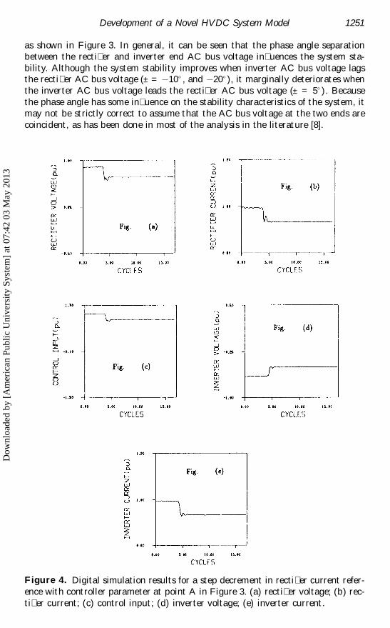
Figure 4. Digital simulation results for a step decrement in recti�er current refer-ence with controller parameter at point A in Figure 3. (a) recti�er voltage; (b) rec-ti�er current; (c) control input; (d) inverter voltage; (e) inverter current.
Dow
nloa
ded
by [
Am
eric
an P
ublic
Uni
vers
ity S
yste
m]
at 0
7:42
03
May
201
3
1252 R. K. Pandey et al.
Validation of the M odel
The stability boundary for ± = 0° in Figure 3 is validated at the points A andC using the dynamic digital simulation program [16]. The simulation results areobtained following a step change in the current reference (1.0 pu to 0.92 pu) atthe recti�er terminal. A corresponding change is also made in the inverter currentsetting to maintain the same current margin. The controller parameters correspond-ing to points A and C are chosen for the simulation purpose. The system responses(recti�er voltage, recti�er current, control input at the recti�er terminal, invertervoltage, and inverter current) are shown in Figures 4 and 5 for points A and C, re-
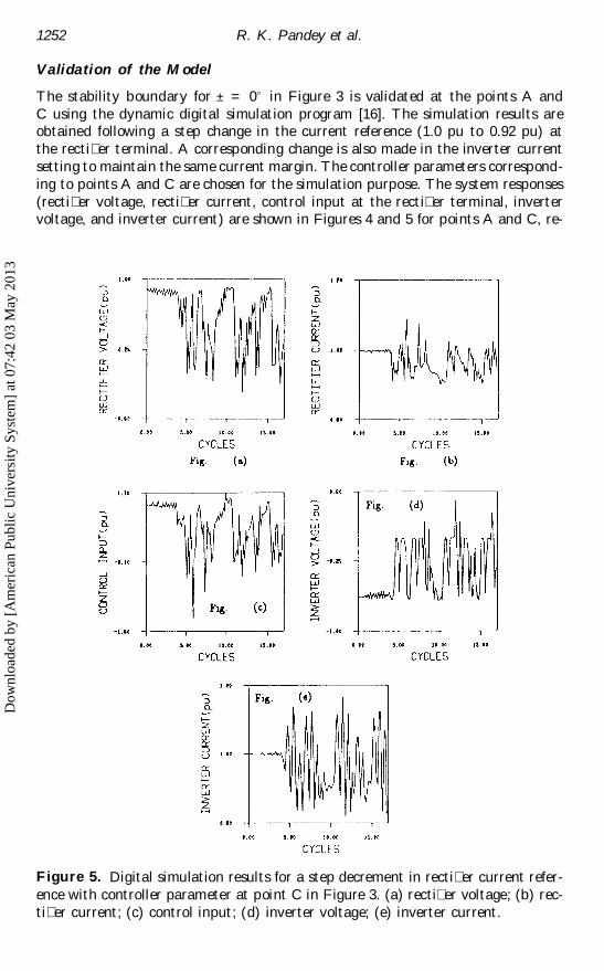
Figure 5. Digital simulation results for a step decrement in recti�er current refer-ence with controller parameter at point C in Figure 3. (a) recti�er voltage; (b) rec-ti�er current; (c) control input; (d) inverter voltage; (e) inverter current.
Dow
nloa
ded
by [
Am
eric
an P
ublic
Uni
vers
ity S
yste
m]
at 0
7:42
03
May
201
3
Development of a Novel HVDC System Model 1253
spectively. The system operation shows a stable behavior with the recti�er currentcontroller parameters corresponding to point A (Fig. 4), whereas very large oscil-lations can be noticed with controller parameters at point C (Fig. 5), indicating anunstable system behavior. It may be mentioned that with the controller parameterscorresponding to point C, the oscillations were so large that the simulation couldnot proceed beyond 17 cycles, as the converter valves ceased conduction at currentzero, which was encountered due to the large oscillations in the current.
EŒect of Extinction Angle
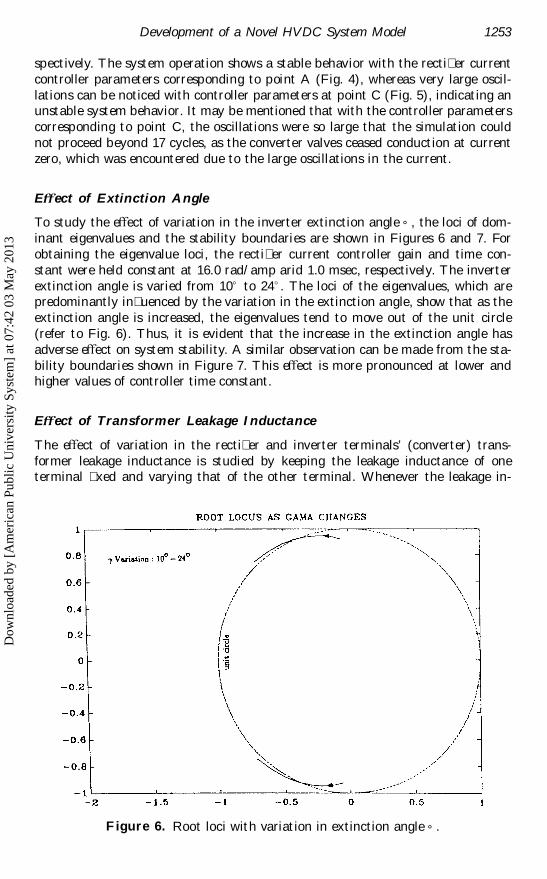
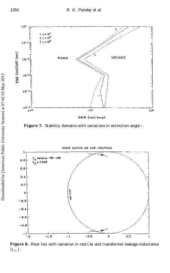
To study the eŒect of variation in the inverter extinction angle ° , the loci of dom-inant eigenvalues and the stability boundaries are shown in Figures 6 and 7. Forobtaining the eigenvalue loci, the recti�er current controller gain and time con-stant were held constant at 16.0 rad/ amp arid 1.0 msec, respectively. The inverterextinction angle is varied from 10° to 24° . The loci of the eigenvalues, which arepredominantly in�uenced by the variation in the extinction angle, show that as theextinction angle is increased, the eigenvalues tend to move out of the unit circle(refer to Fig. 6). Thus, it is evident that the increase in the extinction angle hasadverse eŒect on system stability. A similar observation can be made from the sta-bility boundaries shown in Figure 7. This eŒect is more pronounced at lower andhigher values of controller time constant.
EŒect of Transformer Leakage Inductance
The eŒect of variation in the recti�er and inverter terminals’ (converter) trans-former leakage inductance is studied by keeping the leakage inductance of oneterminal �xed and varying that of the other terminal. Whenever the leakage in-
Figure 6. Root loci with variation in extinction angle ° .
Dow
nloa
ded
by [
Am
eric
an P
ublic
Uni
vers
ity S
yste
m]
at 0
7:42
03
May
201
3
1254 R. K. Pandey et al.
Figure 7. Stability domains with variations in extinction angle ° .
Figure 8. Root loci with variation in recti�er end transformer leakage inductance(L cr ).
Dow
nloa
ded
by [
Am
eric
an P
ublic
Uni
vers
ity S
yste
m]
at 0
7:42
03
May
201
3
Development of a Novel HVDC System Model 1255
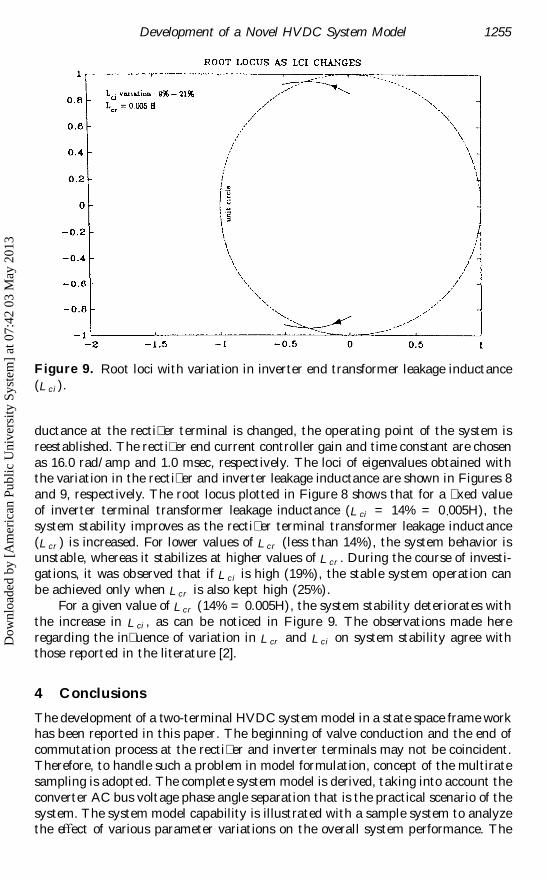
Figure 9. Root loci with variation in inverter end transformer leakage inductance(L c i).
ductance at the recti�er terminal is changed, the operating point of the system isreestablished. The recti�er end current controller gain and time constant are chosenas 16.0 rad/ amp and 1.0 msec, respectively. The loci of eigenvalues obtained withthe variation in the recti�er and inverter leakage inductance are shown in Figures 8and 9, respectively. The root locus plotted in Figure 8 shows that for a �xed valueof inverter terminal transformer leakage inductance (L ci = 14% = 0.005H), thesystem stability improves as the recti�er terminal transformer leakage inductance(L cr ) is increased. For lower values of L cr (less than 14%), the system behavior isunstable, whereas it stabilizes at higher values of L cr . During the course of investi-gations, it was observed that if L c i is high (19%), the stable system operation canbe achieved only when L cr is also kept high (25%).
For a given value of L cr (14% = 0.005H), the system stability deteriorates withthe increase in L ci , as can be noticed in Figure 9. The observations made hereregarding the in�uence of variation in L cr and L c i on system stability agree withthose reported in the literature [2].
4 Conclusions
The development of a two-terminal HVDC system model in a state space frame workhas been reported in this paper. The beginning of valve conduction and the end ofcommutation process at the recti�er and inverter terminals may not be coincident.Therefore, to handle such a problem in model formulation, concept of the multiratesampling is adopted. The complete system model is derived, taking into account theconverter AC bus voltage phase angle separation that is the practical scenario of thesystem. The system model capability is illustrated with a sample system to analyzethe eŒect of various parameter variations on the overall system performance. The
Dow
nloa
ded
by [
Am
eric
an P
ublic
Uni
vers
ity S
yste
m]
at 0
7:42
03
May
201
3

1256 R. K. Pandey et al.
predictions obtained from the study are validated further with the dynamic digitalsimulation in order to give support to the results obtained.
References
[1] Eriksson, K., Liss, G., and Persson, E. V., 1970, “Stability of the control system forHVDC transmission analysis using theoretically calculated nyquist diagrams,” IEEETrans., PAS–89, pp. 733–740.
[2] Carrol, D. P., and Krause, P. C., 1970, “Stability analysis of a DC power system,”IEEE Trans., PAS-89, 1112–1119.
[3] Fallside, F., and Farmer, A. R., 1967, “ Ripple instability in closed loop control systemswith thyristor ampli�ers,” Proc. Inst. Electr. Eng., 114, 139–152.
[4] Parrish, P. A., and McVey, E. S., 1967, “A theoretical model for single phase siliconcontrolled recti�er systems,” IEEE Trans., AC-12, 577–579.
[5] Hazell, P. A., and Flower, J. O., 1970, “Stability properties of certain thyristor bridgecontrol systems: Pt. I-The thyristor bridge as a discrete control system,” Proc. Inst.Electr. Eng., 117, 1405–1412.
[6] Sucena-Paiva, J. P., Hernadez, R., and Freris, L. L., 1972, “Stability Study of Con-trolled Recti�ers Using a New Discrete Model,” Proc. Inst. Electr. Eng., 119, 1285–1293.
[7] Sucena-Paiva, J. P., and Freris, L. L., 1973, “Stability of a DC transmission linkbetween strong AC systems,” Proc. Inst. Electr. Eng., 120, 1233–1243.
[8] Sucena-Paiva, J. P., and Freris, L. L., 1974, “Stability of a DC transmission linkbetween weak AC systems,” Proc. Inst. Electr. Eng., 121, 508–515.
[9] Padiyar, K. R., and Sachchidanand, 1985, “Stability of converter control for multi-terminal HVDC systems,” IEEE Trans., PAS-104, 690–696.
[10] Pandey, R. K., Sachchidanand, and Ghosh, A., 1989, “Multirate sampling basedHVDC converter model,” IEEE Midwest Symp. on Circuits and Systems, Illinois.
[11] Pandey, R. K., Arindam Ghosh and Sachchidanand, 1990, “Two terminal HVDCsystem model for converter control stability analysis based on multirate sampling,”Electric Power Systems Research, 19, 145–154.
[12] Padiyar, K. R., 1990, “ HVDC power transmission system,” Wiely Eastern Limited,New Delhi.
[13] Kimbark, E. W., 1971, “Direct current transmission,” Vol. 1, Wiley, New York.[14] Hingorani, N. G., and Chadwick, P., 1968, “A new constant extinction angle control
for AC/ DC/ AC static converters,” IEEE Trans. PAS-87, 866–872.[15] Kuo, B. C., 1981, “Digital Control Systems,” Holt, Rinehart and Winston, New York.[16] Padiyar, K. R., Sachchidanand, Kothari, A. G., Bhattacharyya, S., and Ajai Srivas-
tava, 1989, “ Study of HVDC controls through e� cient dynamic digital simulation ofconverters,” IEEE Trans., PWRD-4, 2171–2178.
[17] Pandey, R. K., 1991, “A discrete-time HVDC system model for stability analysisand self-tuning control design,” Ph.D. Thesis, Dept. of Electrical Engineering, IndianInstitute of Technology Kanpur, India.
Appendix
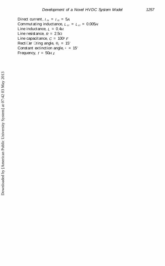
The operating conditions and the parameters of the sample system used for stabilityanalysis are as follows:
No load recti�er direct voltage, Vdr 0 = 100VNo load inverter direct voltage, Vdi0 = 74.636V
Dow
nloa
ded
by [
Am
eric
an P
ublic
Uni
vers
ity S
yste
m]
at 0
7:42
03
May
201
3
Development of a Novel HVDC System Model 1257
Direct current, Idr = Idi = 5ACommutating inductance, L cr = L c i = 0.005HLine inductance, L = 0.4HLine resistance, R = 2.5WLine capacitance, C = 100¹FRecti�er �ring angle, ®r = 15°
Constant extinction angle, ° = 15°
Frequency, f = 50H z
Dow
nloa
ded
by [
Am
eric
an P
ublic
Uni
vers
ity S
yste
m]
at 0
7:42
03
May
201
3