DEVELOPMENT OF A COMPUTER-AIDED

ACCELERATED DURABILITY TESTING METHOD FOR

GROUND VEHICLE COMPONENTS

By

A. K. M. Shafiullah

A Thesis Submitted to the Faculty of Graduate Studies of

The University of Manitoba

In partial fulfilment of the requirements of the degree of

MASTER OF SCIENCE

Department of Mechanical and Manufacturing Engineering

University of Manitoba

Winnipeg, Manitoba

Copyright © 2012 by A. K. M. Shafiullah

i

Abstract

Presently in ground vehicle industries, conducting durability tests with a high

acceleration factor have become increasingly demanding for the less time and cost

involvement. In the previous work, to accelerate the field test, the standard ‘test tailoring’

approach has been modified due to the requirement of high acceleration factors and the

limitations of testing implementation. In this study, a computer-aided testing method is

developed for the validation of this modified approach. Hence, a new test-piece has been

designed by a conjugative approach involving the finite element technique and fatigue

analysis. Afterwards, the accelerated durability loading profiles synthesized via the

modified approach have been applied on the designed test-piece and the fatigue life has

been simulated to verify the effectiveness of those loading profiles. Simulation results

show that loading profiles with an acceleration factor up to 330 can be successfully

generated with an accuracy of 95% by this modified approach.

ii

Acknowledgements

I would like to express my sincere gratitude to my advisor, Dr. Christine Q. Wu for the

guidance to carry out this work. I deeply appreciate for her valuable time, patience and

insight throughout the course of this work. This thesis would not have been possible

without the help and support she has given towards me. Thank you Dr. Wu.

Along with my advisor I would like to thank Dr. Olanrewaju Ojo and Dr. Dagmar

Svecova for serving my committee. I would like to express my appreciation for their

valuable suggestions to improve this work. I also like to thank Dr. Neil Popplewell for

providing me the fundamental background knowledge of vibration and make me

interested to work better in this field.

I am also thankful to Mr. Brad Lamothe from the ‘Motor Coach Industries’, Mr. Steve

Swiddle and Mr. Ken Carmichael from the ‘WESTEST’ for their technical support in this

work. I would also like to thank my colleagues Ms. Ke Xu, Mr. Sushil Doranga, and Mr.

Ehsan Jalayeri for their help in preparing the materials for the tests.

Last but not the least I would like to thank my friends and family for their enormous

support. Specially, I would like to thank my wife for her inspiration, without which I

could not have achieved my goals.

iii

Dedication

I would like to show my heartiest gratitude to my parents for the sacrifices they made for

me and for always believing in me.

iv

Table of Contents

Abstract i

Acknowledgements ii

Dedication iii

Table of Contents iv

List of Figures vi

List of Tables ix

Nomenclature xi

1. Introduction 01

1.1. Accelerated Durability (AD) Tests 01

1.2. Literature Survey 03

1.3. Problem Statement 08

1.4. Objective and Problem Formulation 09

1.5. Organization 11

2. Computer-Aided Accelerated Durability Test- Methodology 12

2.1. Synthesizing AD Testing Loading Profiles 12

2.2. Development of the CAM With Specific Dynamic

Features and Fatigue Life 19

2.2.1. Numerical Vibration and Stress Analysis of the Specimen 19

2.2.2. Experiments for Vibration and Stress Analysis 21

v

2.3. FE Based Numerical Fatigue Analysis and the Verification of the

Synthesized AD Loading Profiles 25

3. Results and Discussion 32

3.1. Synthesized Highly AD Profiles, FDS And ERS Comparison 32

3.2. Design of the Test-Piece and Its Validation 36

3.2.1. Features of the Designed Test-piece 36

3.2.2. Determination of the Dynamic Parameters of the System 39

3.2.3. Comparison between Numerical and Experimental Result 41

3.2.4. Dynamics and Stress Analysis of the CAM 44

3.2.5. Stress Relation with the Fatigue Life 52

3.3. Verification of the AF of the developed AD Tests 55

3.3.1. Numerical Fatigue test and Validation 55

3.3.2. Experimental Durability Tests and Fractography 57

3.3.3. Effect of Plasticity and S-N Curve Slope in

Durability Test Life 61

4. Conclusions and Future Works 69

References 71

Appendix A- Details of the all Considered Test-Piece and their Comparison with the

Selected One 77

Appendix B- Other Fatigue Results 85

Appendix C- Miscellaneous Findings While Generating the AD Test 88

vi

List of Figures

Title Page No

Figure 1: Pennsylvania Testing Facility 02

Figure 2: Shaker Machines Used in Durability Tests 03

Figure 3: The Process Flow Of Generating AD Profiles From nCode

GlyphWorks

16

Figure 4: (a) Road Test Acceleration Data (Z-Vertical Direction) and

(b) Geometry of the Seven Events

18

Figure 5: Meshed CAD with Solid Elements with a Finer Mesh around the

Critical Notches

21

Figure 6: The Experimental Setup: (a) Hydraulic Shaker with the

Mounted Specimens (b) The Data Acquisition System

23

Figure 7: Beams with Attached (a) Strain Gauges and (b) Accelerometer

and Tip Mass

24

Figure 8: Attached Strain Gauges and their Locations in the Designed

Specimen Used for the Test with the 24 Hours Accelerated PSD

24

Figure 9: S-N Curve Formulation for Aluminum 6061 T651 Alloy 28

Figure 10: Vibration Fatigue Process Flow in DesignLife 30

Figure 11: Process Flow of AD Testing Methodology 31

Figure 12: Generated AD Tests of Different Duration for Constant a FDS 33

Figure 13: Response Spectra for Different AD Tests for Constant a FDS 34

Figure 14: Damage Spectra for Different AD Tests for Constant a FDS 35

Figure 15: Notch Orientations of the Designed Specimen (Top-View) 37

Figure 16: (a) The Physical Test-Piece (b) The Test-Piece with Sensors, for

the Experimental Comparisons

38

Figure 17: Linearity Approximation around the Resonance 40

Figure 18: Sample Vibration Time History From the Test-Piece 41

vii

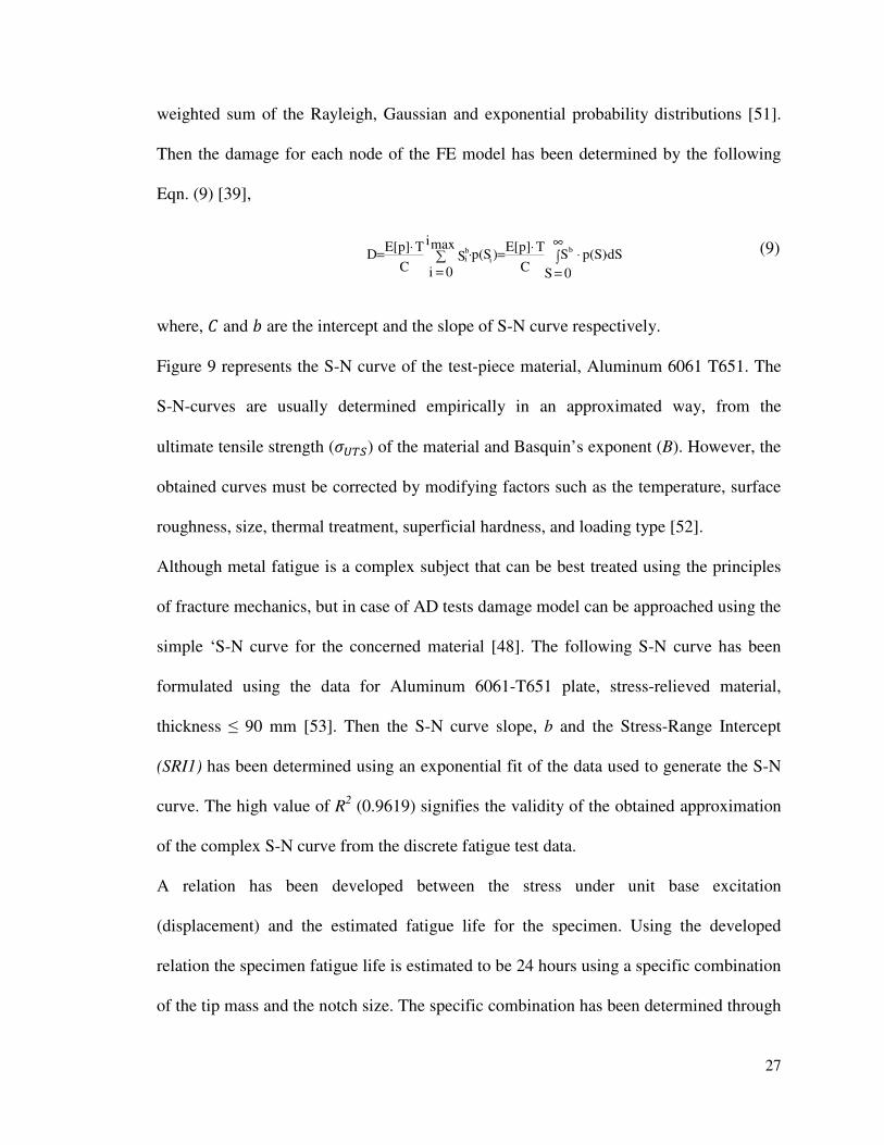
Figure 19: First Four Vibration Modes of the Specimen 45

Figure 20: Experimental Sine Sweep FRF Spectra 46

Figure 21: Von Mises Strains at First Four Natural Frequencies of the

Specimen

47

Figure 22: Von Mises Stress Distribution Over the Model 48

Figure 23: Stress/Strain Distributions for the 4 Hours PSD Over the

Critical Region

50

Figure 24: The Stress PSD Determined From the FEA 51

Figure 25: Relation between the Absolute Maximum Principal Stress and

the Durability Life

53

Figure 26: Effect of the Notch Orientations to the Different Stress

Transfer Functions

54

Figure 27: Effect of the End Masses to the Different Stress

Transfer Functions

54

Figure 28: Fatigue Life Distribution over the CAM for 20 Hours PSD 56

Figure 29: Fatigue Life Distributions over the CAM for Different

Accelerated PSD

57

Figure 30: Failure of the Designed Test-Piece (Experimental) 58

Figure 31:(a) Fracture Surfaces of the Failed Test-Pieces 59

(b) Fracture Surfaces of the Failed Test-Pieces under Optical

the Microscope

60

Figure 32: The Strain History of an Overly Compressed Durability

Loading Profile

64

Figure 33: Comparison of the TC Ratio of Different AD Profiles With the

Theoretical One

66

Figure 34: Deviation in the Determined Fatigue Life for Different

TC Ratios

67

Appendix Section

Figure 1A: Comparison of the Natural Frequencies between the FE and

the Experiment

81

viii

Figure 2A: Attached Strain Gauges in Differently Designed Specimens 81

Figure 3A: Comparison of Strain Results between the FE and

The Experiment

83

Figure 4A: Response Spectra of Different AD Tests for Constant

FDS (b=6)

88

Figure 5A: Damage Spectrums of Different AD Tests for Constant

FDS (b=6)

89

Figure 6A: Response Spectra for Different AD Tests (Full) for

Constant ERS (b=6)

90

Figure 7A: FDS for Different AD Tests (Full) For Constant ERS (b=6) 91

ix

List of Tables

Title Page No

Table 1: Range of Values of ‘b’ for Different Materials 14

Table 2: The Natural Frequencies And the Damping Ratios for the First Two

Vibration Modes for Different Specimens

39

Table 3: Comparison of the Natural Frequencies between the FE and

the Experimental Model

42

Table 4: Comparison of Strains between the FE and the Experimental

Model for the 24 Hours Loading Profile

42

Table 5: The Comparison of Maximum Tip Deflections between the FEA

the Experiment

43

Table 6: Comparisons of the RMS Stresses (1-Sigma) Over the CAM 49

Table 7: Verification of the Synthesized AD Tests (�=6) 56

Table 8: Natural Frequencies and Damping Ratios for the First Two

Bending Vibration Modes for the Different Specimens

61

Table 9: Comparison of Strains between the FE and the Experiments for

Beam Set 2

62

Table 10: Verification of the Synthesized AD Tests (b=5.5) 65

Appendix Section

Table 1A: Fatigue Lives of the Different Test-Pieces under the 24 Hours

Loading

77

Table 2A: The Natural Frequencies and the Damping Ratios for the First

Two Bending Modes for Different Specimens (Experimental)

78

Table 3A: Gain Ratios of the First Two Bending Modes (Experimental) 78

Table 4A: Strains Developed in the 24 Hours Durability Test in 79

x

the FE Models

Table 5A: Comparison of the Natural frequencies between the FE and

the Experimental Model

80

Table 6A: Comparison of Strains between the FEA and the Experiment 82

Table 7A: Comparison of Strain Distributions between the FEA

and the Experiments

84

Table 8A: Fatigue Lives in Different Locations of the Specimens Based on

Experiments

85

Table 9A: Estimated Fatigue Life of the Four Selected Specimens Using

Different Cycle Counting Algorithms in the Frequency Domain

86

xi

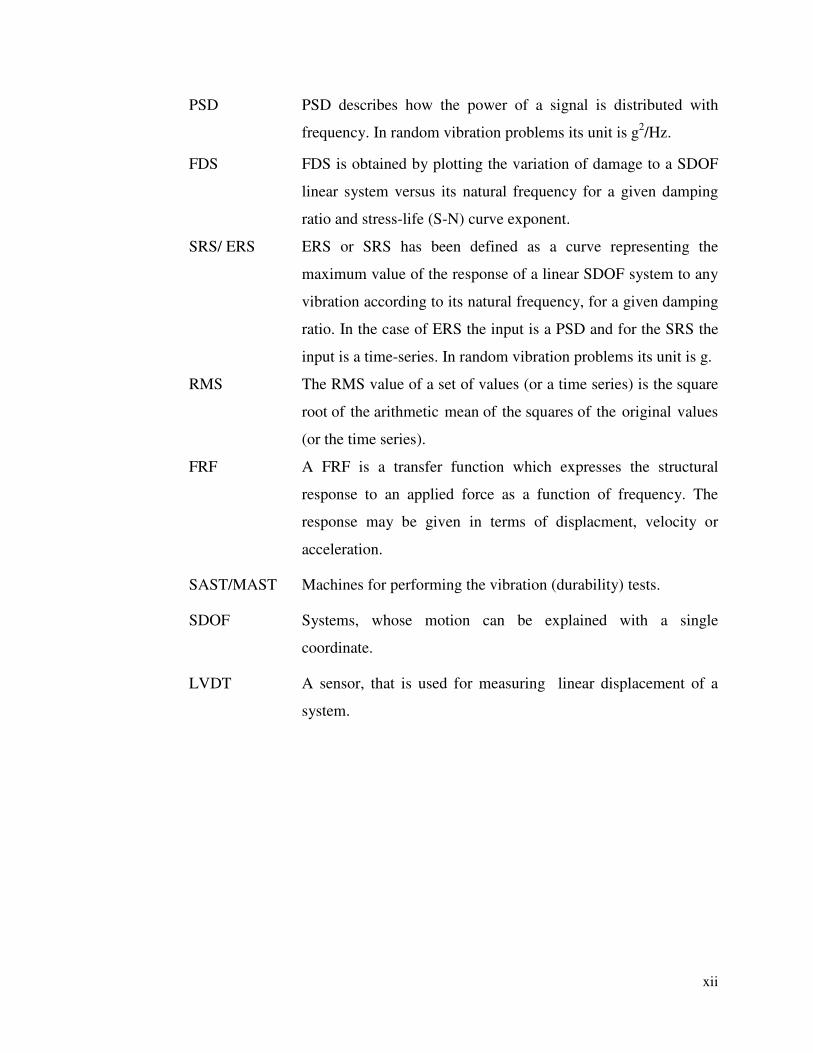
Nomenclature

1. Acronyms

AD Accelerated Durability

AF Acceleration Factor

CAE Computer-Aided Engineering

CAM/ CAD Computer-Aided Model/Design

FEA Finite Element Analysis

FDS Fatigue Damage Spectrum

FRF Frequecy Response Function

FE Finite Element

FLR Fatigue Life Ratio

LVDT Linear Variable Differential Transformer

PSD Power Spectral Density

RMS Root Mean Square

S-N Stress Life

SRS/ ERS Shock/ Extreme Response Spectrum

SAST/MAST Single/Multi Axis Simulation Table

SDOF Single Degree Of Freedom

2. Definitions for Selected Acronyms

FLR The ratio of the fatigue life of a specific specimen under the

original load and the accelerated load.

LES A system whose deformation under load is assumed to be linear

elastic.

AF AF is the ratio of the duration of the original (field) test and the

duration of the accelerated test.

xii

PSD PSD describes how the power of a signal is distributed with

frequency. In random vibration problems its unit is g2/Hz.

FDS FDS is obtained by plotting the variation of damage to a SDOF

linear system versus its natural frequency for a given damping

ratio and stress-life (S-N) curve exponent.

SRS/ ERS ERS or SRS has been defined as a curve representing the

maximum value of the response of a linear SDOF system to any

vibration according to its natural frequency, for a given damping

ratio. In the case of ERS the input is a PSD and for the SRS the

input is a time-series. In random vibration problems its unit is g.

RMS The RMS value of a set of values (or a time series) is the square

root of the arithmetic mean of the squares of the original values

(or the time series).

FRF A FRF is a transfer function which expresses the structural

response to an applied force as a function of frequency. The

response may be given in terms of displacment, velocity or

acceleration.

SAST/MAST Machines for performing the vibration (durability) tests.

SDOF Systems, whose motion can be explained with a single

coordinate.

LVDT A sensor, that is used for measuring linear displacement of a

system.

1

Chapter 1

Introduction

1.1. Accelerated Durability (AD) Tests

Ground vehicles must pass the durability tests as a pre-launch requirement to meet the

necessary standards for the safety, reliability, durability and comfort. These durability

tests (field tests) are usually conducted in the proving grounds, which are designed to

simulate the real road environments (events) during the tests. A map of a typical

durability testing facility at Pennsylvania Transportation Institute has been presented in

Figure 1 [1]. During the durability tests the ground vehicles need to be driven a certain

amount of mileage without exhibiting any failure mechanism including any crack

initiation in critical suspension, frame and cab systems to certify the marketability of the

vehicle [2]. Hence, these durability assessments also possess the risk of nullifying the

invested time and money, if any of the components of the driven vehicle fails during the

test.

As an alternate, AD test can be designed for the laboratories to simulate the driving

conditions of the field tests in a shorter period of time. An effective accelerated lab test

not only helps avoid the unexpected failures during the field tests but also can be used to

quantify the life span of ground vehicle components with less investment of time and

money. Moreover, information regarding the determination of the warranty timeframe of

2

the vehicle components to minimize the product recalls and complaints after marketing

can be obtained once the AD test is conducted [2]. The benefit of AD tests over the field

test is that it can be better reproduced and observed, as the individual vehicle component

can be tested under the controlled environment rather than the full vehicle prototype.

However, the challenge exists as the loads to be used in the rig test (controlled

environment) have to be derived based on the measurements performed either on the test

tracks or in the public roads [3].

Figure 1: Pennsylvania Testing Facility [1]

A proficient AD test should satisfy the following two criteria [2]:

1. The AD test should produce the same failure mechanism as those observed in the real-

world loading conditions, i.e., being representative of the real loading environments.

2. The AD test should be accelerated with no occurrence of the unrealistic high load

which can possibly alter the response of the structure hence the failure mechanism.

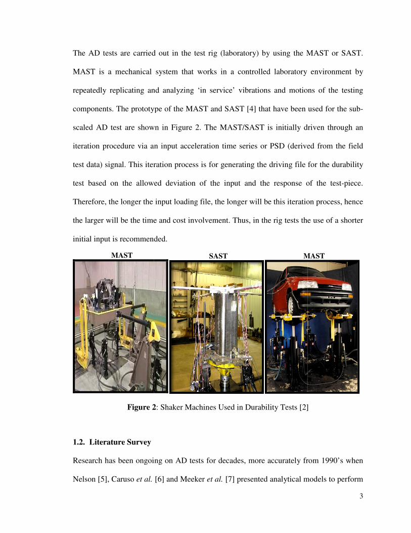
The AD tests are carried out in the test rig

MAST is a mechanical system that works in a controlled

repeatedly replicating and analyzing

components. The prototype of the MAST and SAST

scaled AD test are shown

iteration procedure via an input acceleration

test data) signal. This iteration process is

test based on the allowed

Therefore, the longer the input

the larger will be the time an

initial input is recommended.

Figure 2

1.2. Literature Survey

Research has been ongoing on AD tests for decades, more accurately from 1990’s when

Nelson [5], Caruso et al.

MAST

carried out in the test rig (laboratory) by using the MAST

MAST is a mechanical system that works in a controlled laboratory environment by

peatedly replicating and analyzing ‘in service’ vibrations and motions of

. The prototype of the MAST and SAST [4] that have been used for the sub

scaled AD test are shown in Figure 2. The MAST/SAST is initially driven

via an input acceleration time series or PSD (derived from the field

. This iteration process is for generating the driving file

the allowed deviation of the input and the response of the

, the longer the input loading file, the longer will be this iteration process

the larger will be the time and cost involvement. Thus, in the rig tests the

recommended.

2: Shaker Machines Used in Durability Tests [2]

Research has been ongoing on AD tests for decades, more accurately from 1990’s when

[6] and Meeker et al. [7] presented analytical models to perform

SAST MAST

3

MAST or SAST.

laboratory environment by

vibrations and motions of the testing

been used for the sub-

driven through an

erived from the field

for the durability

deviation of the input and the response of the test-piece.

iteration process, hence

the use of a shorter

[2]

Research has been ongoing on AD tests for decades, more accurately from 1990’s when

analytical models to perform

MAST

4

the accelerated tests. In 1992, Ashmore et al. [8] demonstrated a procedure to perform

accelerated tests in the test course which can be treated as the first guideline to perform

the AD test for ground vehicles. They explored the effect of critical test parameters (the

test field roughness severity and the vehicle speed in the test course) on the AF and also

verified their assumptions of the method to get valid results. More techniques have been

introduced afterwards to accelerate the reliability or durability field tests. Briefly these

techniques have been categorized as the time-domain-based or the frequency-domain-

based approaches. Earlier techniques have been accelerating the durability tests mostly in

the time domain.

Time-domain-based techniques include short-inverse-Fourier transform (SIFT) [9], time

correlated fatigue damage (TCFD) [10], strain gauge editing technique (SGET) [11]-[13]

and racetrack editing technique (RTET) [14]. All these techniques [9]-[14] are broadly

termed as the ‘fatigue damage editing’, which is a signal processing technique. In such a

technique, the signal (the time-history of the strain, acceleration, and displacement) is

collected from the field tests via sensors like strain gauges, accelerometers, LVDTs, etc

and edited to retain the desired percentage of the damaging portion of the signal. In these

techniques [9]-[14], non-damaging or less damaging parts (according to the S-N curve of

the material) are removed from the signal hence accelerate the tests. To perform the test

in the laboratory, the edited signal is correlated with the acceleration or the displacement

of the shaker machines [12]. ‘Mildly Non-Stationary Mission Synthesis’ (MNMS) which

is a time-domain-based signal processing technique, produces shorter mission signals

from long records of experimental data [15]. In [15] the MNMS technique is

demonstrated up to an AF of 10 and found to be efficient in low AF (1 to 3). Broadly, the

5

time-domain-based techniques are reliable as it deals with the real time data without any

transformation. Moreover, the theories are well established and a lot of experimental data

is also available in the time-domain-based techniques. However, the AF cannot be truly

controlled in these techniques since the AF mostly depends upon the severity of the

acceleration, displacement or strain data collected from the durability track [9]-[15].

Moreover, in [16] the experimental and numerical techniques (FE transient analysis) are

blended together as an efficient and reliable means for performing the dynamic response

and the durability analysis of heavy commercial vehicles. The transient analysis in time-

domain becomes computationally expensive if the considered analysis time is large or the

system is complex comparing to frequency-domain-based computational methods [17].

Hence, it can be also concluded that the time-domain-based techniques cost more

computational time and machine memory than the frequency-domain-based techniques.

The earliest complete literature has been found practising the frequency-domain-based

approach for fatigue life prediction of metallic structure in 1986 by Bishop [18]. This

approach has been refined with computer-aided techniques, i.e. FE has been incorporated

[19] [20] to perform the durability analysis of machine components in a more convenient

way. For the random vibration problems, the methodology of performing the durability

analysis of mechanical/electronic components in the frequency domain have been

presented in [21]-[27]. The techniques used here have been tailored from [18] and [20].

In these works, durability assessments have been carried out using a combination of FE

random vibration and numerical fatigue analysis. Furthermore, in [28] the spectral

damage of a ‘Linear Elastic System’ (LES) has been predicted in the frequency domain

using a novel approach of energy isoclines, whose function consists of both FRF and the

6

material fatigue properties of that system. Later, to reduce the testing time, frequency-

domain-based durability tests have been accelerated using different techniques.

Literature that addressed accelerating the field test using the frequency-domain-based

techniques can be found in [29]-[44]. In literature [29]-[33], to accelerate the test, the

RMS values of the test PSD have been increased; hence higher stress levels have been

developed in the structure to make it fail faster. In these cases, the RMS values have been

found to be arbitrarily increased [29]-[32] or it has been increased by using the inverse

power law [33]. In [29] the acceleration level (g) of the vibration test profiles has been

elevated and applied to differently damped (coated) cantilever beams to determine the

effect of damping on the AF of the considered vibration test profiles. In some cases the

temperature loading profile also has been accelerated by elevating its RMS level to

account the temperature effect along with the vibration loading while performing the

bench test on a metallic component (the catalytic converter) [30]. In [31] and [32] the

accelerated test has been performed in aluminum beams with elevated RMS level of the

test PSD. In these works, the effect of the damping co-efficient [31] and the effect of

different cycle counting algorithms (Dirlik, Narrowband, Steinberg, Lalanne etc) [32] on

the fatigue lives of cantilever beams has been analysed. However, these techniques [29]-

[33] have not been accounted for the impact failure or the failure mechanism alteration

while accelerating the test. Some other techniques have also been proposed in the

literature [34]-[36]. A ‘step-stress accelerated random vibration life testing method’ has

been presented to accelerate the test in [34]. An analytical solution has been presented to

calculate the fatigue damage for a linear elastic SDOF system which has been used as the

specifications of the accelerated vibration tests [35]. Moreover literature have been found

7

which addressed the usage of inverse power laws in the accelerated fatigue testing under

wide-band Gaussian random loading [36]. These techniques [34]-[36] are more on the

theoretical side and not yet been exercised in the practical applications.

In 2006, Halfpenny [37] proposed a novel approach, the ‘test tailoring approach’ of

accelerating the durability tests. In this technique, the AF can be controlled up to the

theoretical limit defined by the Condition 1. This technique also contains the algorithm

to avoid impact failures in high AF. The ‘test tailoring approach’ is consisting of two

steps, (1) mission profiling and (2) test synthesis. Mission profiling involves determining

the SRS and the FDS from the field test data by applying a SDOF transfer function to the

input acceleration signal (field test acceleration data). The calculation is repeated over a

range of natural frequencies to give histograms of maximum response and fatigue against

the frequency. The ‘test synthesis’ process in the ‘test tailoring approach’ accelerates the

field test using the information (FDS and SRS) of the mission profiling. The conditions

of generating AD loading profiles through the ‘test tailoring approach’ can be briefly

described as below,

Condition 1: ERS of the accelerated test must be below the SRS of the road/field test to

avoid creating unrealistic load which may cause impact/shock failure.

Condition 2: FDS of the accelerated test must be same as the FDS of the road/field test

to ensure the same failure mechanism.

So in this approach, accelerated test profiles are obtained by synthesizing a field test PSD

with a same damage potential of FDS, while bounding the solution with SRS and ERS

[38].

8

Halfpenny in 2008 [39], also embedded the ‘test tailoring approach’ with CAE, where the

combination of generating the durability loading profiles and testing those in the test rig

has been elaborated [39]. The ‘test tailoring approach’ has also been applied in the

aviation applications [40]-[42], accelerating a 12000-hour field test to a 4-hour lab test to

evaluate the durability of the helicopter components in uni-axial [41] and tri-axial

directions [42]. In [40] the ‘test tailoring approach’ has been exercised to perform a

numerical AD test of an automobile component. None of these works [40]-[42] validated

the claimed AF of the generated loading profiles used in their durability analysis.

Xu et al. [43] and Cull et al. [44] also applied the ‘test tailoring approach’ to generate

accelerated loading profiles for the durability tests of ground vehicle components. In [43]

the damaging events of the field test acceleration data have been identified successfully

for the ‘mission profiling’ process and later accelerated the field test via the ‘test

synthesis’ technique. Prior to this work, the framework has been established in [44] for

generating these successful AD loading profiles using the commercial software nCode

GlyphWorks. This methodology has been refined and adopted in [43] to synthesise

effective AD loading profiles in [44].

1.3. Problem Statement

Field test data of 330 hours, collected from Altoona test track [1] needs to be accelerated

to perform a 24-hours equivalent (or less) lab test through any existing or new approach.

The challenges of this works are described as follows:

1. To accelerate the concerned 330-hour test keeping all the dynamic features of the

field test, where the conventional ‘test tailoring approach’ was exceeding the

theoretical limit defined by Condition 1.

9

2. To generate an equivalent 60s acceleration time series from the 24-hours accelerated

test PSD (of the 330-hour test) which can be repeated for 1440 times to get the

desired FDS. This equivalent 60s time series must be produced for the rig tests to

reduce the time and cost involved in the iteration process with the full period tests

(e.g. 24-hour test).

Hence, to accelerate the field test, in [43] the standard ‘test tailoring approach’ has been

modified’ to obtain the desired AF (e.g. the AF of accelerating the 330 hours field test to

24 hours is 13.75) and to satisfy the Condition 1 and 2 for implementation. To apply this

new modified approach to industrial durability tests, it needs to be validated.

Furthermore, in this modified approach some assumptions have been made on the

important dynamic properties of the considered SDOF system [43], which should be

verified to validate the framework adopted in [43].

1.4. Objective and Problem Formulation

This work is mainly focused on verifying the ‘modified test tailoring approach’ of

generating the AD loading profiles for ground vehicle components presented in [43]. The

significance of this work is to develop a tool which can potentially provide the guideline

for the ground vehicle manufacturers to perform numerical AD tests complimentary to

the expensive field or lab testing. The objectives of this work can be categorized in the

following manner:

1. To synthesize AD loading profiles of higher AF (>13.75) from the considered 330-

hours of field test through the ‘modified test tailoring approach’. A different S-N

curve slope and FDS generating algorithm than the previous work [43] have been

chosen to accelerate the AD loading profiles of shorter duration in this work.

10

2. Designing a new test-piece having specific dynamic features and fatigue life to

perform the numerical and experimental durability tests.

3. Validation of the AF of the synthesized AD loading profiles and the verification of

consistent fatigue mechanism resulted for performing fatigue/durability assessment

with those loading profiles. i.e., validation of the ‘modified test tailoring approach’.

4. Presenting a guideline for performing a valid AD test both in the test-rig and in

numerical techniques with the existing Altoona field [1] test data.

In this work, AD loading profile has been synthesized through ‘modified test tailoring

approach’ via commercial software nCode GlyphWorks [45]. This approach consists of

two distinguished techniques termed as ‘Mission Profiling’ and ‘Test Synthesis’. Mission

Profiling generates the reference SRS and FDS from the Altoona field [1] test

acceleration data. In addition, via ‘Test Synthesis’ technique the AD loading profiles are

obtained by synthesizing a field test PSD with a same damage potential of FDS, while

bounding the solution with SRS and ERS. Furthermore, a new featured test-piece has

been designed by a conjugative approach involving the FEA and the fatigue analysis (S-

N analysis) for a specific fatigue or durability life. The design is validated afterwards to

perform the durability tests and verify the AF of the applied durability test profiles. In

this case, to perform the FEA, and the fatigue analysis, Education Version of ANSYS

13.0 [46] and nCode DesignLife 7.0 [47] has been used in this work. Ideally the

durability or FLR should be same as the AF of the considered AD loading profiles.

Hence, the FLR and the AF for every applied AD profiles have been compared to

validate the effectiveness of the synthesized AD loading profiles. Experiments have also

11

been performed to validate failure mechanism of AD loading profiles to signify the

numerical results.

1.5. Organization

In Chapter 2, the methodology computer-aided AD test has been discussed. In the first

part of the computer-aided AD test, Section 2.1, the method and materials of the

synthesized AD tests are presented, where the PSD of the AD loading profiles have been

generated with the corresponding SRS and FDS satisfying the Condition 1 and 2,

discussed in Section 1.2. In the second part of computer-aided AD test, Section 2.2, the

design techniques of the test piece having a specific durability life of 24 hours are

presented through FEA and the standard fatigue analysis. The 24-hour duration has been

taken as a reference and it is the preferred applicable durability test, to simulate the 330

hour of the field test. Experiments which have been performed to validate the design are

also presented in this section. In the third part of the computer-aided AD test, Section 2.3,

the synthesized AD loading profiles have been applied to the CAM of the test-piece and

the corresponding fatigue life has been determined. Later, the FLR and the AF for every

AD profiles have been compared to validate the effectiveness of the synthesized AD

loading profiles. Results and discussions are presented in Chapter 3. In this chapter the

feature of the synthesized AD loading profiles (PSD, SRS and FDS) and the designed

test-piece (material, geometry, boundary condition, dynamics and fatigue life) have been

presented. The validations of the test-piece’s design and the generated AD loading

profiles have also been demonstrated in this chapter. Conclusions and the future works

are presented in Chapter 4. References and appendices are appended afterwards.

12

Chapter 2

Computer- Aided Accelerated Durability Test-Methodology

This work has three major parts. They are synthesizing the AD loading profiles using the

‘modified test tailoring approach’, designing a specific dynamically featured test-piece or

specimen with a certain fatigue life and testing the specimen under the generated AD

profiles to verify their effectiveness. Such effectiveness has been defined as the

consistency between the AF and the FLR, which is referred as the ratio of the fatigue life

of a specific specimen under the original load and the accelerated load. The considered

AD loading profiles have been synthesized from 330 hours of field test to 24, 20, 15, 10,

8, 6, 4, 2 and 1 hour via the modified approach with the identical data and the parameters

presented in literature [43] using the commercial software nCode GlyphWorks. Nine (9)

AD loading profiles have been synthesized in this work to provide enough information

for the validation.

2.1. Synthesizing AD Testing Loading Profiles

The main objective of AD testing is to reduce the time of the conventional durability tests

without altering failure mechanism. In frequency-domain-based techniques, the vibration

test is usually accelerated by elevating the stress level [33]. In this process, the reference

vibration loading profile, which needs to be accelerated, is in the form of a PSD. The

relationship between the PSD levels and the test durations is given as [41],

13

1

2B/n

2

1

T

T)

W

W( = (1)

where, ��and �� are the field and accelerated laboratory test PSD amplitudes (g2/Hz),

respectively, �� and �� are the field and laboratory test durations in hours, respectively, �

is the inverse slope of the Wohler curve (S-N curve) or the Basquin’s exponent and � is

the stress damping constant. In Eqn. (1) � and � are the material properties.

In this work the AD loading profile has been generated from the field test data through

the ‘modified test tailoring approach’. The ‘test tailoring approach’ has been developed

based on a SDOF system. The first stage of the ‘test tailoring approach’ is the mission

profiling, where the SRS and the FDS of the field test data is determined by the following

formulations [39],

2

1

nnnn T)]ln(f)PSD(fQf[π)ERS(f ⋅⋅⋅⋅⋅= (2)

)2

bΓ(1]

)f2(2π

)PSD(fQ[

C

KTf)FDS(f 2

b

3n

nb

nn +⋅⋅

⋅⋅⋅⋅= (3)

where, is the spring stiffness of the SDOF system, � is the natural frequency of the

SDOF system, � is the time period of the accelerated test, � is the dynamic amplification

factor, ��(�) is the power spectral density of the input acceleration, �(�) is the

Gamma function defined by�(�) = � �(���)∞

�∙ ��� ∙ ��, � and � are the slope and the

intercept of the S-N curve respectively, where the S-N curve is defined by � = ∙ �!

where, is the no of cycles to failure of cyclic stress amplitude � .

The second stage of the ‘test tailoring approach’ is the ‘test synthesis’, where the AD

loading profiles (PSD) are generated using the following Eqn. (4) [39]. During the ‘test

14

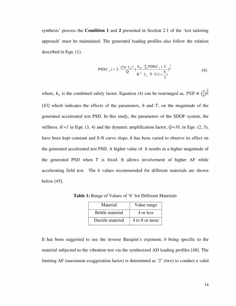
synthesis’ process the Condition 1 and 2 presented in Section 2.1 of the ‘test tailoring

approach’ must be maintained. The generated loading profiles also follow the relation

described in Eqn. (1).

b

2

nb

n3

nn ]

)2

bΓ(1TfK

C)FDS(fck[

Q)f(2π

2)PSD(f+⋅⋅⋅

∑ ⋅⋅⋅⋅=

where, "# is the combined safety factor. Equation (4) can be rearranged as, �� ∝ (�

%)&'

[43] which indicates the effects of the parameters, � and�, on the magnitude of the

generated accelerated test PSD. In this study, the parameters of the SDOF system, the

stiffness, =1 in Eqn. (3, 4) and the dynamic amplification factor, �=10, in Eqn. (2, 3),

have been kept constant and S-N curve slope, � has been varied to observe its effect on

the generated accelerated test PSD. A higher value of � results in a higher magnitude of

the generated PSD when � is fixed. It allows involvement of higher AF while

accelerating field test. The b values recommended for different materials are shown

below [45].

Table 1: Range of Values of ‘b’ for Different Materials

It has been suggested to use the inverse Basquin’s exponent, b being specific to the

material subjected to the vibration test via the synthesized AD loading profiles [48]. The

limiting AF (maximum exaggeration factor) is determined as ‘2’ (two) to conduct a valid

Material Value range

Brittle material 4 or less

Ductile material 4 to 8 or more

(4)

15

durability test in the test rigs [49]. The exaggeration factor is defined as the ratio of the

PSD level of the accelerated test and the road test.

In this work, the ‘modified test tailoring approach’ [43] has been developed to generate

the durability loading profiles to perform accelerated tests. In the modified approach, the

acceleration time series of a duration of 60s is extracted using the inverse Fourier

transformation (IFT) from the full period accelerated PSD, which is synthesized via the

‘test synthesis’ process of the standard ‘test tailoring approach’ [43]. This equivalent 60s

loading profile (time series) is termed as the partial test loading profile and it must have

the similar pattern and contain the same dynamic features of the field test. As the RMS

value of the full period test is certain times ( () of the one of the partial test, the loading

profile of the partial test is repeated for ( times to obtain the desired FDS as the full

period test. The number of recurrence( () is calculated using Eqn. (5)

pfr /TTN = (5)

where, �) and �* are the durations of the full and partial periods of the accelerated

durability tests respectively.

The other benefit of the partial testing is that it allows higher time compression than the

full period AD loading profiles. Hence partial tests help in generating highly AD loading

profiles for the industrial durability testing. The process-flow of generating the full period

AD loading profiles and partial tests, using nCode GlyphWorks, has been presented in

Figure 3.

For this work, the field test acceleration data has been collected via a tri-axial

accelerometer from the front axle of the test vehicle driven in the Altoona proving ground

[1]. This proving ground is designed to simulate the real road conditions during the

16

field/road test of the heavy ground vehicles. The collected 694 seconds acceleration data

from the field test includes six laps and every lap contains seven different road events [2].

Figure 4 represents the field test acceleration data (sample) and the geometries of the

seven road events of the durability track. In this case, the ground vehicles are required to

drive 6250 miles without any failure in the main components [44].

Figure 3: The Process Flow of Generating AD Profiles Using

nCode GlyphWorks

As a first step of the modified approach, all of the seven (7) events have been

successfully identified from the collected acceleration data [43]. Then using the

acceleration data of each event, the SRS and the FDS of the field test have been

developed through the ‘mission profiling’ technique. From this FDS of the field test data,

the AD loading profiles of full duration period have been synthesized by the ‘test

5

1

2

6

7 8

4 3

17

syntheses’ technique. Later, the partial test has been obtained by filtering the full period

test PSD by the white noise of duration of 60 seconds (60s). Later, the ERS and the

equivalent FDS of the partial test have been determined and compared against the field

test SRS and FDS to validate the synthesized partial tests. Here the equivalent FDS is

determined by multiplying the recurrence number( () with the FDS of the 60s partial

test. To satisfy the Condition 2, presented in Chapter 1 the equivalent FDS determined

from the accelerated partial tests have been kept the same as the FDS of the field test to

ensure the same failure mechanism.

Moreover, the ERS of the partial test has been compared against the SRS of the field test.

To satisfy the Condition 1 mentioned in Chapter 1 the ERS of the synthesized partial

tests have been kept lower than the field test SRS to avoid the alteration of the failure

mechanism. As this work is based on the modified approach [43], the ERS of the partial

test, instead of the ERS of the full period test has been compared with the SRS of the

field test.

In GlyphWorks, the process starts with the ‘Test Synthesis Glyph’ (marked as ‘1’) where

the FDS of the field test determined via the mission profiling technique has been fed and

the full test AD loading profile has been obtained as output (‘Full Period AD Test’,

marked as ‘2’) after the synthesis process. Afterwards, the full period AD test has been

filtered (marked as ‘6’) by white noise of 60s duration to get the partial test loading

profile (MAST/SAST driving file). To confirm a valid AD test, the ERS and the

equivalent FDS of the ‘Partial Test PSD’ (marked as ‘5’) have been compared (marked as

‘7’ and ‘8’) with those of the field test. The equivalent FDS is found by multiplying

(marked as ‘4’) the FDS of the partial test (marked by ‘3’) by the recurrence no.

18

Figure 4: (a) Road Test Acceleration Data (Z-Vertical Direction) and (b) Geometry of

the Seven Events

100 200 300 400 500 600 700

-1

-0.5

0

0.5

1

Time, Seconds

Nor

mal

ised

Acc

eler

atio

n, g

(a)

(b)

5. Railway crossing

19

2.2. Development of the CAM with Specific Dynamic Features and Fatigue Life

A cantilever beam has been designed to demonstrate a computer-aided AD test and to

validate the modified process of generating the highly compressed AD tests for the

ground vehicle components. In this work, cantilever beams have been chosen for its well

established mathematical model. The criteria of designing the test piece are as follows:

• The dominant vibration mode must be a bending mode and the natural frequency of

this mode should be close to 7 Hz. It is crucial as it is the first natural frequency of

the suspension system of the considered ground vehicles.

• The lateral vibration mode must be least dominant if it lies in the frequency

bandwidth of 0-60 Hz. The specimen should have a very low tendency to vibrate in

lateral directions because only the vertical excitation is applied.

• The fatigue life of the specimen should be 24 hours under the reference loading

which is developed based on the modified procedure presented in [43].

The design process involves, (1) FEA along with a standard fatigue analysis (S-N) to

obtain the specific durability life span of the cantilever beam and (2) experiments to

verify the dynamic characteristics of the designed test-piece.

2.2.1. Numerical Vibration and Stress Analysis of the Specimen

The objective of the FEA is to analyze the dynamic response and the stresses of the test-

piece. Firstly, the FE model has been developed in SOLIDWORKS. The geometry file is

then imported to ANSYS. SOLID 95 elements have been used for meshing the

SOLIDWORKS model. Approximately 150,000 elements have been used in the meshed

model and it has been shown in Figure 5. The primary assumptions used in FEA are as

follows:

20

• The model is linear and the material is homogeneous and linear elastic;

• The damping ratio is constant as 2%, temperature and humidity effects are negligible

Aluminum 6061-T651 alloy has been selected for the beam. Different notch orientations

(cross section) and tip mass combinations have been analyzed to find the specimen with

the desired frequencies and mode shapes. The modal analysis has been performed using

software ANSYS through ‘ANSYS Parametric Design Language’.

In this work, the cantilever beams have been placed horizontally and experienced the

vertical acceleration to its fixed end. Hence, to achieve the structural responses

(displacements and strains) both random vibration analysis and harmonic response

analysis has been performed through ANSYS. The modal analysis is a pre-requisite to

both of the above mentioned analyses, therefore the same boundary conditions, material

properties, meshing, damping properties of modal analysis are applicable to both

harmonic response analysis and random vibration analysis.

The random vibration analysis in ANSYS is capable of solving the base excitation

problem using PSD as an input. Stress or displacement results are determined as a PSD in

the probabilistic manner following the normal distribution through this analysis. On the

other hand, as ANSYS is not capable of providing unit acceleration while performing

harmonic response analysis, unit displacement have been used instead of the acceleration

through coupled degree of freedom to excite the base. Considering a linear SDOF system,

the stress response of the specimen can be obtained for different input. To determine the

response PSD for a particular input PSD, the FRF results of the harmonic response

analysis has been used as shown in Eqn. (6) [42]. This stress PSD has been used as the

input for the fatigue analysis.

21

Figure 5: Meshed CAD with Solid Elements with a Finer Mesh around the Critical

Notches

(f)G(f)h(f)q

i

q

jh(f)G ij

*jiyy ⋅⋅∑∑=

where, +,,() and +-.() are the output and input PSD to the system and ℎ() is the

transfer function of the system. ‘*’ is used to represent the complex conjugate of the

transfer function [42]. The results from FEA are then passed to the commercial software

nCode DesignLife for performing the fatigue analysis of the designed test-piece.

2.2.2. Experiments for Vibration and Stress Analysis

Performed FEA has been verified by the experiments as the CAM (FE model) needs to be

used in the numerical fatigue analysis. Parameters, e.g., damping, linearity of the

specimen and the response of the SAST to the input have also been obtained through

experiments. The test procedure comprises of ‘sine sweep tests’ in three different

Fixed end

Top view

Isometric view

X

Z

X

Y

(6)

22

frequency ranges in the 3-65 Hz bandwidth and a 5-minute durability test with the partial

tests extracted from the selected 24, 20, 4 and 1 hours accelerated PSD.

Here, The three sine sweep trials have been, 0.1g peak to peak at 0.5 octaves per minute

in the range of 3-65 Hz (test-a), 0.2g peak to peak at 0.1 octaves per minute in the range

of 3-8 Hz (test-b) and 0.2g peak to peak at 0.1 octaves per minute in the range of 45-65

Hz (test-c). The main objective of performing the sine sweep test is to determine the

natural frequencies in the range of 0-60 Hz and the damping present in the system.

In the experiment, the specimens, placed horizontally, have been subjected to vertical

vibration through the SAST [4]. This SAST is run by the hydraulic power by means of

the MTS actuator series 206. This actuator has a moving mass of 16.8 kg. The fixture

having a mass of 21.12 kg has been attached to the actuator which yields the total moving

mass of the shaker to 37.92 kg without the specimens attached. While attaching the

specimens (cantilever beams) to the fixture, an 88 N-m torque has been applied. Prior

starting the test it has been verified through the iterative technique that the shaker table

can implement the loading provided, with a very least amount of deviation, i.e. RMS

deviation less than 4%.

One 4393 type piezoelectric uniaxial charge accelerometer has been attached at the tip of

each attached beam to collect the acceleration response of the beam. This accelerometer

is chosen for its very low weight (4 gm with magnet attached) and very high shock

absorbing capacity (±25000g). An accelerometer of the same type is also attached to the

fixture to get the response acceleration of the actuator or the base. Figure 6, shows the

hydraulic shaker/SAST and all the four specimens mounted in the fixture (a) and the data

acquisition system (Somat eDaq Plus) (b) to collect and store the data that was received

23

from the transducers.

Figure 6: The Experimental Setup: (a) Hydraulic Shaker with the Mounted Specimens

(b) The Data Acquisition system

Also six strain rosettes (CEA-13-062UR-350) and five axial strain gauges (two EA-

031DE-350/E and three EA-062DN-350/E) have also been attached to different locations

of the beams to collect the strain histories. Figure 7 shows the physical beam with the

strain gauges, tip mass and accelerometer attached. Before starting the test, the

accelerometers and the strain gauges have been calibrated to the required scale of the data

acquisition system. After every trial the residual stresses have been recorded and

calibrated to zero for the convenience of the analysis. The data acquisition system is

capable of collecting data from 36 channels simultaneously. Data has been collected at a

sampling rate of 2500 Hz which is around 39 times of the maximum frequency of the

loading applied to the system. A 60s loading profile from the reference loading has been

used to perform a 5-minute durability test. The profile has been repeated for five (5)

times to generate more consistent strain data. ‘Remote Parameter Control’ (RPC)

(a) (b)

Fixture

Hydraulic Actuator

24

software has been used to apply the loading to the SAST. As the iteration process

becomes expensive using the full period AD loading profile, the representative 60s time

series has been used.

Figure 7: Beams with Attached (a) Strain Gauges and (b) Accelerometer and Tip Mass

Figure 8: Attached Strain Gauges and their Locations in the Designed Specimen Used

for the Test with the-24 Hours Accelerated PSD

Figure 8 presents the locations of the strain gauges attached to the designed beams. Strain

Cantilever Beams

Accelerometer

Tip Mass

Strain Gauges (a) (b)

25

data has been collected during this 5-minute durability test to compare the experimental

strains (maximum equivalent Von Mises) with the strain results found from the random

vibration analysis performed on the FE model. The natural frequencies that were found

from the sine sweep test will also be compared with those from the FE model. After

verification, fatigue analysis is performed on the model based on the results of FEA.

Furthermore, by double integrating the filtered (via a high pass filter, threshold is 3 Hz)

tip response acceleration data, the displacement history of the tip of the beam has been

obtained. Using the tip displacement history and the length of the beam the angular

deviation history of the tip of the beam from the horizontal axis has been determined.

Afterwards, the maximum angular deviation has been compared with that of the FEA to

verify the soundness of the FE model. Linearity in the response of the beam has also been

discussed from the angular deviation data.

2.3. FE Based Numerical Fatigue Analysis and the Verification of the Synthesized

AD Loading Profiles

There are two distinct reasons for performing the numerical fatigue analysis. They are:

• To design a dynamically featured test-piece for approximately 24 hours of fatigue life

(Significance level0 ≤ 0.05).

• To determine the FLR of the designed test-piece for different AD loading profiles

which are synthesized in this work and verify their effectiveness.

The FRF results (displacements, stresses and strains under the unit base excitation) of the

CAM have been determined through the harmonic response analysis and transferred to

nCode DesignLife for the fatigue analysis. In the case of heavy ground vehicles, the

stress-life (S-N) method is very effective to be used in the determination of the durability

26

[50]. Hence, in this work, to determine the durability or the fatigue life of the test-piece,

the S-N fatigue analysis has been performed in the frequency domain.

For the S-N method the stress information (stress-time histories or stress PSDs) needs to

be separated to the stress ranges and the number of stress reversals. The Rainflow Cycle

Counting Algorithm and ‘Dirlik’, ‘Narrowband’, ‘Lalanne’, ‘Steinberg’ algorithms can

be used to perform this separation [51] in the time-domain-based and the frequency-

domain-based S-N method, respectively. Afterwards, using the material’s S-N data, the

damage for each stress/strain reversal is determined and the accumulated damage is

calculated according to Miner’s law to find out the total damage. In the previous

literature it has been found that Dirlik’s algorithm is the most consistent with the

‘Rainflow cycle algorithm’ [17]. Hence, ‘Dirlik’s’ algorithm has been widely used to

perform the frequency-domain-based fatigue analysis. In this work, ‘Dirlik’s’ algorithm

has been used to design the final specimen as well. The mathematical model of the

‘Dirlik’s is as follows [39],

p(S)TE[p]N(S) ⋅⋅= (7)

where, (�) is the number of the stress cycles of range � (MPa) expected in time � (s),

5[7] is the expected number of peaks and probability density function of stress range � is

as follows,

0

2

3

2

2

2

2

λ

2Z

eZD2RZ

eR

ZDQZ

eQ1D

p(S)

−⋅⋅+

−⋅+

−

⋅

= (8)

Parameters ��, ��, �:, ;, <= and > can be determined from the respective mathematical

formulations [28] prescribed by Dirlik. The Dirlik Eqn. (7 and 8) is based on the

27

weighted sum of the Rayleigh, Gaussian and exponential probability distributions [51].

Then the damage for each node of the FE model has been determined by the following

Eqn. (9) [39],

dS

0S

p(S)SC

TE[p])p(S

maxi

0iS

C

TE[p]D b

ibi ⋅∫

∞

=

⋅⋅

=⋅∑=

⋅= (9)

where, � and � are the intercept and the slope of S-N curve respectively.

Figure 9 represents the S-N curve of the test-piece material, Aluminum 6061 T651. The

S-N-curves are usually determined empirically in an approximated way, from the

ultimate tensile strength (?@%A) of the material and Basquin’s exponent (B). However, the

obtained curves must be corrected by modifying factors such as the temperature, surface

roughness, size, thermal treatment, superficial hardness, and loading type [52].

Although metal fatigue is a complex subject that can be best treated using the principles

of fracture mechanics, but in case of AD tests damage model can be approached using the

simple ‘S-N curve for the concerned material [48]. The following S-N curve has been

formulated using the data for Aluminum 6061-T651 plate, stress-relieved material,

thickness ≤ 90 mm [53]. Then the S-N curve slope, b and the Stress-Range Intercept

(SRI1) has been determined using an exponential fit of the data used to generate the S-N

curve. The high value of R2 (0.9619) signifies the validity of the obtained approximation

of the complex S-N curve from the discrete fatigue test data.

A relation has been developed between the stress under unit base excitation

(displacement) and the estimated fatigue life for the specimen. Using the developed

relation the specimen fatigue life is estimated to be 24 hours using a specific combination

of the tip mass and the notch size. The specific combination has been determined through

28

the trial and error technique. While developing the relationship, the maximum absolute

principal stress has been determined from a consistent location irrespective to the notch

sizes/orientations and tip mass combinations. To determine the maximum absolute

principal stress, the harmonic response analysis has been performed for the amplitude of

1 meter (unit displacement in the SI system) sinusoidal base excitation in the 0-60 Hz

frequency bandwidth with a frequency step of 0.2 Hz. As this stress analysis has been

performed for the unit excitation, it has been termed as the transfer function of stress

transfer function (Pa/m).

Figure 9: S-N Curve Formulation for Aluminum 6061 T651 Alloy

Validation of the ‘modified test tailoring approach’ presented in [43] has been performed

by testing the designed specimen with the synthesized AD loading profiles. Theoretically,

for a successful AD test the AF should be equal to the FLR of the specimen. To

determine the fatigue life, the result file (.rst) of ANSYS containing the FRF results has

y = 8E+08x-0.109

R² = 0.9619

5.0E+07

5.0E+08

5E+02 5E+03 5E+04 5E+05 5E+06 5E+07 5E+08

Str

ess

Ran

ge,

Pa

No of Cycles to Fail

Series1

Trendline SN

Curve (Adopted)

29

been imported to nCode DesignLife and the fatigue life has been determined for all

synthesized AD loading profiles using frequency-domain-based S-N method. The

absolute maximum principal stress has been used as the stress invariant as the mean bi-

axiality ratio, ‘r’, which is in the range of -1˂r˂ 0 [54]. While determining the maximum

absolute principal stress from the experimental strains, the transverse sensitivity of the

gauges, 1, 2 and 3 of the rosettes have been taken as 0.012, 0.006 and 0.012 [55]. Dirlik

algorithm [39] has been used to separate the absolute maximum principal stress PSD to

the stress ranges, the number of stress reversals, and Goodman criteria has been used to

correct the existing mean stress. As the level of AD loading profiles has a unit of ‘g’ and

the stress transfer functions has an unit of ‘Pa/m’, to make the units consistent, the AD

loading profiles have been integrated twice and converted to the displacement spectrum

density before using it in the fatigue analysis [56]. Finally, the expected fatigue life and

the estimated fatigue life of the developed model have been compared. The process flow

of vibration fatigue analysis performed via nCode DesignLife has been presented below

in Figure 10.

In this process it has been shown that the ‘FE FRF Results Glyph’ (marked as ‘1’) and

the displacement PSD (‘FFT’ (Fast Fourier Transform), marked as ‘2’) of the 60s partial

test has been used as the input to the ‘Vibration CAE Glyph’ (‘Vibration Fatigue

Analysis’, marked as ‘3’) for the fatigue analysis. Proper material, algorithms and the

loading information have also been imported into this glyph for performing a standard S-

N analysis to obtain the ‘Fatigue Life Distribution Glyph’ (marked as ‘4’) in the model.

The displacement PSD has been found by double integrating the acceleration signal of

the partial test. Filtering has also been performed before the integration process to

30

remove the frequency content less than 3 Hz because the SAST/MAST cannot implement

any frequency below this limit. Output of the process can be found in the ‘Fatigue Life

Distribution Glyph’, and the ‘Data Glyph’ (marked as ‘5’).

Figure 10: Vibration Fatigue Process Flow in DesignLife

In Figure 11, the design process of the test-piece has been described via a flow. It

summarizes the techniques used in this chapter. The total flow divided into two analyses

boxes for better understanding. They are ‘AD Testing and FE Analysis’ and the ‘FE

based Fatigue Analysis’. Detail of these two analyses can found within the boxes.

Combining the results of these two analyses the test-piece has been designed via a trial

and error method.

1 3

2

4

5

31

Figure 11: Process Flow of AD Testing Methodology

AD Testing and FE Analysis

FE based Fatigue

Analysis

32

Chapter 3

Results and Discussion

This section consists of three subsections. In Section 3.1, results from the ‘modified test

tailoring approach’ have been presented. In Section 3.2, the design of the test-piece has

been presented with its featured results and experimental validation. Section 3.3 presents

the numerical durability analysis results to validate the generated AD loading profiles

hence the ‘modified test tailoring approach’.

3.1. Synthesized Highly AD Profiles, FDS and ERS Comparison

Features of AD loading profiles generated via ‘modified test tailoring approach’ have

been presented in this section. These loading profiles have been synthesised from 330

hours of field test data. In Figure 12, full period AD test profiles of different duration

(1.5, 2, 4, 8, 10, 15, 20 and 24 hours) have been demonstrated. These AD loading profiles

have been shown in a form of PSD against frequency in a bandwidth of 0-60 Hz. The

amplitude of the PSD is expressed in ‘g2/Hz’, where, ‘g’ is the gravitational acceleration.

It is found that for all of the accelerated profiles, the level of the PSD gets higher when

the duration of the test has been shortened. These loading profiles also keep the similar

trends for the frequency components to ensure the same failure mechanism. Moreover, all

of the PSD this figure show a peak around 7.25 Hz, which represents the natural

frequency of the suspension systems of the vehicle under study.

33

Figure 12: Generated AD Tests of Different Duration for a Constant FDS

These synthesized AD loading profiles can be used as the input to the SAST/MAST in

two forms: 1) a PSD or equivalent time series of a full test period, and 2) an equivalent

60s time series. For implementation, the second method is recommended to save the cost

and time involved in the iterative process of generating the driving files for the

SAST/MAST [57]. Hence, the partial tests have been generated from the full period tests.

As the partial tests are implemented in the durability tests, the ERS and equivalent FDS

of the partial test has been compared with the SRS and FDS of the field test. The

0 10 20 30 40 50 6010

-7

10-6

10-5

10-4

10-3

10-2

10-1

Frequency, Hz

PSD

Lev

el, g

2 / H

z

Reference PSD(24 hours)1.5 hours PSD2 hours PSD4 hours PSD8 hours PSD10 hours PSD15 hours PSD20 hours PSD

34

equivalent FDS is determined by multiplying the recurrence number( () (Eqn. 5) with

the FDS of the 60s partial test.

Figure 13: Response Spectra for Different AD Tests for a Constant FDS

Figure 13 represents the comparison of the ERS of the partial test profiles synthesized via

modified approach with the SRS of the field test. The amplitude of the ERS is expressed

in ‘g’, the gravitational acceleration. It has been shown that levels of all the ERS (g) are

below the SRS of the field test. Therefore, the synthesized durability loading profiles

have not caused any impact failure or alternation of the failure mechanism of the

0 10 20 30 40 50 600

0.5

1

1.5

2

2.5

3

3.5

Frequency, Hz

Acc

eler

atio

n, g

Field test SRS1.5 hour ERS2 hour ERS4 hour ERS8 hour ERS10 hour ERS15 hour ERS24 hour ERS

35

structure. The bandwidth of 0-60 Hz has been chosen because after 60 Hz the response of

the components of the ground vehicles is very low.

Figure 14: Damage Spectra for Different AD Tests for a Constant FDS

Equivalent FDS of the synthesized partial AD loading profiles via modified approach and

the field test has been presented in Figure 14. Here, the partial tests (of 60s) have been

repeated for ‘Nr’ times to cause the same damage as of the full period tests, i.e., to make

the durations of the full period test and the partial test the same. Then the FDS of the field

test and the equivalent FDS of the partial test have been compared. Figure 14 shows that

the equivalent FDS of all of the partial accelerated profiles almost overlap with the FDS

0 10 20 30 40 50 6010

-20

10-15

10-10

10-5

100

Frequency, Hz

Dam

age

Field test FDS1.5 hour FDS2 hour FDS4 hour FDS8 hour FDS10 hour FDS15 hour FDS24 hour FDS

Rel

ativ

e D

amag

e S

pect

rum

Lev

el

36

of the field test. Thus the modified approach guarantees the consistence between the

failure mechanisms for all the AD loading profiles, which is the most important feature of

an accelerated test. In Figure 14, the damage is presented in log-scale along the Y axis as

the damage is very low comparing to the linear scale. It has also been observed from

Figure 12 and Figure 14 that in the frequency range of 25-60 Hz, the level of the

accelerated PSD is low to cause any significant damage (< 10��D) to the considered

system. Some deviation on the FDS of the AD profiles with the field test has been

observed between 50-55 Hz. This deviation has negligible effect on the durability process

as the level of accelerated PSD (Figure 12) in this frequency range is low.

Hence, the field test may be accelerated to any durations within the upper-bound keeping

the same damage mechanism using the ‘modified test tailoring approach’. The Upper-

bound is determined by the SRS of the field tests. Thus this approach eliminates the risk

of high AF which can alter the failure mechanism. It can be concluded that the AF is

much more controlled in this ‘modified test tailoring approach’ then other existing

techniques. Importantly, the modified approach is valid up to linear elastic region of the

considered system.

3.2. Design of the Test-Piece and Its Validation

The features of the designed test-piece, its experimental validation and the iterative

technique of the design process have been presented in this section.

3.2.1. Features of the Designed Test-Piece

The features of the designed test-piece satisfying the criterion discussed in Section 2.2 has

been summerized as follows with the notch orientations shown in Figure 15.

37

38.1

mm19 mm

75 mm

20 mm

30 mm20 mm

R8

mm

R3.5m

m

R7

mmR8 m

m

15 mm

25 mm

R7.

11 m

m

275.4 mm

101.6 mm

R6

mm

R7

mm

R6 mm

45°

R7.11 mm

1. Type of the structure Cantilever beam

2. Material Aluminum 6061 T651

3. Cantilever length 73 cm

4. Cross section 12.7 cm x 0.79 cm

5. Tip mass 251 gm

6. Fatigue life under the reference loading 23.8 hours(estimated)

Figure 15: Notch Orientations of the Designed Specimen (Top-View)

Figure 16 shows (a) the physical test-piece attached to the fixture, (b) the same test-piece

with the attached sensors for experimental strain collection. Two sets of beams of the

same design configuration have been fabricated for the experimental validation.

These sets have beam fabricated in different places. First set (4 beams) of the beams have

been manufactured earlier for the validation of the design and the second set (12 beams)

has been fabricated later to perform the experimental durability tests to verify the AF of

the synthesized AD loading profiles. The number of beams is a multiple integer of 4

(four) because the fixture has been built to hold maximum 4 specimens at a time. Test-

pieces have been subjected to sine sweep tests and trial durability tests with 24, 20, 8 and

1 hour accelerated PSD. All the trial durability tests have been performed for 5 minutes.

38

To collect the strains, one rosette and two axial strain gauges have been attached in the

location R_1, A_1 and A_2 respectively which are shown in Figure 16(a).

Figure 16: (a) The Physical Test-Piece (b) The Test-Piece with Sensors, for the

Experimental Comparisons

R_1

A_1 A_2

(b)

(a)

39

3.2.2. Determination of the Dynamic Parameters of the System

In this section, important dynamic properties, i.e. the natural frequencies, damping

coefficients and linear response behaviors of the designed test-piece have been

experimentally determined. Table 1 summarizes the averaged results found from the

three performed logarithmic-sine sweep tests presented in Section 2.2. From these test

results, two vibration (bending) modes have been found within the frequency bandwidth

of 0-60 Hz. As the acceleration data has been collected only for the vertical direction, no

lateral vibration mode (second vibration mode) can be obtained from this experimental

acceleration data. It is also observable from the experimental results that the first bending

mode is, at an average, 3.5 times more dominant than the second one. Hence the damping

ratio of the first mode is considered as the constant damping (0.2053%) throughout the

FEA [25].

Table 2: The Natural Frequencies and the Damping Ratios for the First Two Vibration

Modes for Different Specimens

Test Set

Natural Frequency of the 1st Mode

(Hz)

Damping Ratio of the

1st Mode (%)

Natural Frequency of the 3rd Mode

(Hz)

Damping Ratio of the 3rd Mode

(%)

Gain Ratio of the 1st and

3rd Mode

1 7.114 0.2053 56.91 0.6857 3.190

Regarding the linearity approximation, around the vicinity of the natural frequencies of

the first two bending modes, structural non-linear response has been observed. Beyond

such vicinity, the specimen behaves closely to a linear system. This phenomenon can be

observed in Figure 17. In this figure, gain ratios between two different base excitations

have been plotted against the frequency. For the linear response of a system, the gain

ratio for different excitation should be unity. In these cases the gain ratio violates this

40

criterion around 7.11 Hz and 56.9 Hz which are the first and third natural frequency of

the specimen.

Figure 17: Linearity Approximation around the Resonance

However, the natural frequency and the damping ratio of the first mode can also be

determined from the free vibration test using the logarithmic decrement rule. As the

natural frequency and the damping ratio of the other vibration modes cannot be retrieved

by this rule, sine sweep tests are necessary to determine the dynamics of the other modes.

Figure 18 shows the free vibration history of the test piece along with the points

considered for applying the logarithmic decrement rule. The exponential envelope

(window) determined from the measured data has been presented in this figure shows

how ideally the damping affects the vibration (response). Using the two points shown in

Figure 18, the natural frequency and the damping ratio of the first mode can be

determined using the fundamental relationships of a SDOF system. Importantly, the

5 6 7 8

0.7

0.8

0.9

1

1.1

1.2

1.3

Frequency, Hz

Gai

n R

atio

52 54 56 58 600.5

0.7

0.9

1.1

1.3

1.5

Frequency, Hz

Gai

n R

atio

41

results determined from the FRF of the sine sweep test and the free vibration test are

close in both quantitative and qualitative sense.

Figure 18: Sample Vibration Time History from the Test-Piece

3.2.3. Comparison between Numerical and Experimental Results

In this section, the FEA and the experimental results have been compared to validate the

design. The damping ratio determined from the experiments has been updated in FEA to

compare strains of FEA with those from the experiments. Table 2 presents a comparison

of the averaged natural frequencies for the first four vibration modes of the test-pieces. It

shows that the maximum deviation between the FEA and the experiments based on the

natural frequency of the first mode is 2.162% and overall the maximum deviation is

5.091% in the fourth mode. Test has also been performed to ensure the convergence of

the FEA results prior to the analysis.

115 119 123 127 131 135-1

-0.5

0

0.5

1

Time, Seconds

Nor

mal

ized

T

ip A

ccel

erat

ion

↓

↓

First Point

Second Point

Measured Data Exponential Window

42

Table 3: Comparison of the Natural Frequencies between the FE and the Experimental

Model

Test Set

Vibration Modes Analytical Natural Frequencies (FE)

Hz

Experimental Natural Frequencies

Hz

Percentage (%) of

deviation

1

First (bending) 7.272 7.114 2.161

Second(transverse) 33.82 N/A -------

Third (bending) 59.66 56.91 4.616

Forth (bending) 174.7 165.8 5.091

Another comparison between the maximum equivalent Von Mises strains from the

experiments and the FEA for the selected locations (Figure 5) is presented in Table 3. An

axial strain gauge is attached at the location A1 and two of the strain rosettes are attached

at locations R1, R2. The maximum deviation in the strain results is found as 2.610% at

the location A1 and the minimum deviation is found as 0.390% at R2. While determining

the maximum Von Mises strains from the FEA, 3 − ? results are considered 99.73% of

the results (data).

Table 4: Comparison of Strains between the FE and the Experimental Model for the 24

Hours Loading Profile

Test Set

Strain Gauges/ Rosettes

Area Averaged FE Strains (3-sigma)

(µε)

Experimental Strains

(µε)

Absolute Deviation in Strains

(%)

1

A1 1416 1454 2.610

R1 984.0 990.6 0.660

R2 1266 1271 0.390

The maximum tip deflections of the cantilever beams (the test-piece) under different AD

43

loading profiles have been compared between the numerical and experimental techniques

in Table 4. In the experiment 24, 4 and 1 hour loading profiles have been implemented.

From these tests, the average deviation in maximum tip displacement has been found as

6.30%. It is observed from the results presented in Table 4, as the duration of the

accelerated PSD gets lower, this deviation becomes higher. The 4 hour and the 1 hour

loading profile have been implemented in a different set of beams (test set 2) which may

have caused the relatively larger deviation in the tip displacements.

In Table 4 the experimental axial angular deviations from the fixed end in the first

vibration mode have been presented. It shows that the maximum angular deviation is 7.42

degree which indicates the non-linearity in the structural response. The maximum angular

deviation has been found to be increasing with the RMS of the accelerated profile.

Analyzing the results from Section 3.2.3, it can be concluded that the CAM truly

represents the physical test-piece as the deviations between the FEA and the experimental

results are low.

Table 5: The Maximum Tip Deflection Comparison between the FEA

and the Experiment

Test Sets

Duration of Accelerated

PSD

(Hours)

Numerical Maximum Tip Displacement

(3-sigma) (cm)

Mean-corrected Experimental Maximum Tip Displacement

(cm)

Percentage (%) of

Deviation in the

Results

Experimental Angular

Deviation with the Fixed end

(degree)

1 24 6.09 6.41 4.99% 5.01

2

04 8.48 7.42 12.5% 5.80

01 10.6 9.12 13.9% 7.12

44

3.2.4. Dynamics and Stress Analysis of the Test-piece

In this section several dynamic features (the mode shapes, tip displacements and

stress/strains) of the designed cantilever beam have been discussed. Firstly, Figure 19

presents the first four mode shapes of the developed CAM of the designed test-piece. The

natural frequencies and the damping ratio of these vibration modes can be obtained

through the sine sweep tests (Table 2). In Figure 20, the FRF results obtained from the

sine sweep tests have been presented. These results (spectra), (a) input acceleration, (b)

response acceleration, (c) coherence, (d) gain of the system, (e) cross spectrum, (f)

inertance and (g) receptance has been plotted against the frequency. Receptance only

describes the response of the system in terms of its displacement amplitudes under the

unit excitation. Velocity and acceleration amplitude can also used as the FRFs which are

known as the mobility and the inertance.

In Figure 20, the gain spectrum (Figure 20(d)) of the system, three distinguished peaks

around 7 Hz, 59 Hz and 174 Hz have been observed. These peaks represent the three

natural frequencies (bending modes) of the test-piece at the given frequency range (0-200

Hz). Furthermore, the coherence (Figure 20(c)) of the signal has been found significant

(very close to unity) at the natural frequencies. In the inertance (Figure 20(d)) and

receptance (Figure 20(d)) spectra the response of the second and third vibration mode

have been insignificant which indicates the first mode of vibration is much more

dominant than the other vibration modes.

45

Figure 19: First Four Vibration Modes of the Specimen

Second mode shape

Third mode shape

Fourth mode shape

First mode shape

Fixed End

Fixed End

Fixed End

Fixed End

46

Figure 20: Experimental Sine Sweep FRF spectra

Figure 21 shows the maximum Von Mises strain distribution in the first four vibration

modes of the test-piece. The locations of the maximum strain of the FE model in those

vibration modes have been encircled in the following figure. In these contour plots, red

and blue color represents the maximum and the minimum of the considered parameter,

respectively. Hence the bar colors blue to red follow the increasing manner of the

contoured parameter. Combining the information of Figure 19 and Figure 21, the possible

location of maximum Von Mises stress in the durability tests can be determined. In this

0 20 40 60 80 100 120 140 160 180 2000

0.01

0.02

0.03

Frequency, HzIn

put,

m/s

2

(a)

0 20 40 60 80 100 120 140 160 180 2000

2

4

Frequency, Hz

Res

pons

e, m

/s2

(b)

0 20 40 60 80 100 120 140 160 180 2000

0.1

0.2

0.3

0.4

Frequency, HzCro

ss s

pect

rum

, (

m/s

2 )2 /Hz

(e)

0 20 40 60 80 100 120 140 160 180 2000

50

100

Frequency, Hz

Gai

n

(d)

0 20 40 60 80 100 120 140 160 180 200-1

-0.5

0

Frequency, Hz

Coh

eren

ce

(c)

0 20 40 60 80 100 120 140 160 180 2000

0.05

0.1

Frequency, Hz

Res

po

nse

, m

/s

(g)

0 20 40 60 80 100 120 140 160 180 2002000

1

2x 10

-3

Frequency, Hz

Res

po

nse

, m

(f)(f) (g)

47

problem, it has already been shown that the first mode is most dominant vibration mode

in the bandwidth of 0-60 Hz. Thus for this mode the maximum strain developed at the

location A which is the most possible maximum stress location in the durability tests in

this frequency band.

Figure 21: Von Mises Strains at First Four Natural Frequencies of the Specimen

Von Mises stress is one of the most popular stress invariant to perform the stress analysis

for the ductile materials. A Von Mises stress contours over the CAM for the 2-hour AD

loading profile has been presented in Figure 22. In this figure the location of maximum

stress in the FE model is shown at the location A, which is consistent with the location

presented in Figure 21. As the stress distributions are qualitatively similar for all AD

loading profiles, only one of them has been presented.

First vibration mode

A

Third vibration mode Fourth vibration mode

Second vibration mode

48

As the geometry of the structure and the loading is symmetric about the plane of

symmetry along the longitudinal axis (mid-plane), the stress distribution is also

symmetric about the mid-plane. Hence, location A and location B or similar points

(equally distant) to the mid-plane should be ideally symmetric regarding the stress

distribution. So most likely the locations A and B are the two most vulnerable locations

to fatigue failure as well.

Figure 22: Von Mises Stress Distribution over the Model

Table 5 shows a comparison among the different stresses developed in the FE model of

the test-piece. The AD loading profiles of 24, 20, 15, 8, 4 and 1-hour are applied to the

Critical Region

(High stress region)

A

B

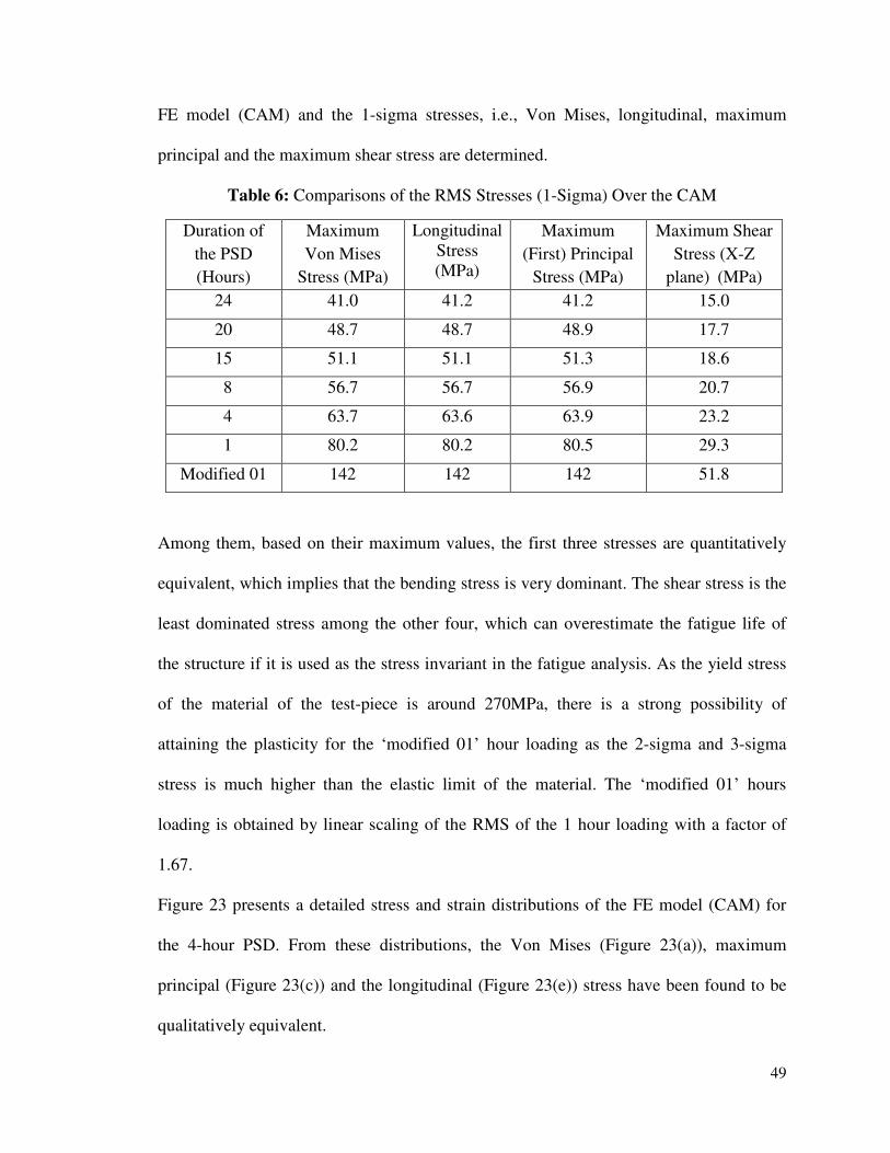
49

FE model (CAM) and the 1-sigma stresses, i.e., Von Mises, longitudinal, maximum

principal and the maximum shear stress are determined.

Table 6: Comparisons of the RMS Stresses (1-Sigma) Over the CAM

Duration of the PSD (Hours)

Maximum Von Mises

Stress (MPa)

Longitudinal Stress (MPa)

Maximum (First) Principal

Stress (MPa)

Maximum Shear Stress (X-Z

plane) (MPa)

24 41.0 41.2 41.2 15.0

20 48.7 48.7 48.9 17.7

15 51.1 51.1 51.3 18.6

8 56.7 56.7 56.9 20.7

4 63.7 63.6 63.9 23.2

1 80.2 80.2 80.5 29.3

Modified 01

142 142 142 51.8

Among them, based on their maximum values, the first three stresses are quantitatively

equivalent, which implies that the bending stress is very dominant. The shear stress is the

least dominated stress among the other four, which can overestimate the fatigue life of

the structure if it is used as the stress invariant in the fatigue analysis. As the yield stress

of the material of the test-piece is around 270MPa, there is a strong possibility of

attaining the plasticity for the ‘modified 01’ hour loading as the 2-sigma and 3-sigma

stress is much higher than the elastic limit of the material. The ‘modified 01’ hours

loading is obtained by linear scaling of the RMS of the 1 hour loading with a factor of

1.67.

Figure 23 presents a detailed stress and strain distributions of the FE model (CAM) for

the 4-hour PSD. From these distributions, the Von Mises (Figure 23(a)), maximum

principal (Figure 23(c)) and the longitudinal (Figure 23(e)) stress have been found to be

qualitatively equivalent.

50

Figure 23: Stress/Strain Distributions for the 4 Hours PSD over the Critical Region

a. Maximum Principal Stress Contours b. Maximum Shear Stress

c. Von Mises Stress Contours d. Von Mises Stress Contours

Normal to Stress Raiser

e. Axial Stress Contours f. Maximum Shear Strain along the ‘Cutting Plane’

‘Cutting Plane’

g. Von Mises Strain Contours

h. Maximum Principal strain

C

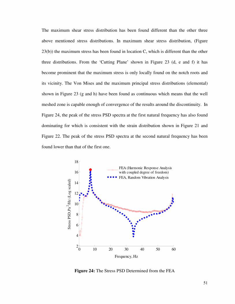
51

The maximum shear stress distribution has been found different than the other three

above mentioned stress distributions. In maximum shear stress distribution, (Figure

23(b)) the maximum stress has been found in location C, which is different than the other

three distributions. From the ‘Cutting Plane’ shown in Figure 23 (d, e and f) it has

become prominent that the maximum stress is only locally found on the notch roots and

its vicinity. The Von Mises and the maximum principal stress distributions (elemental)

shown in Figure 23 (g and h) have been found as continuous which means that the well

meshed zone is capable enough of convergence of the results around the discontinuity. In

Figure 24, the peak of the stress PSD spectra at the first natural frequency has also found

dominating for which is consistent with the strain distribution shown in Figure 21 and

Figure 22. The peak of the stress PSD spectra at the second natural frequency has been

found lower than that of the first one.

Figure 24: The Stress PSD Determined from the FEA

0 10 20 30 40 50 602

4

6

8

10

12

14

16

18

Frequency, Hz

Str

ess

PS

D,P

a2/H

z (L

og s

cale

d)

FEA (Harmonic Response Analysiswith coupled degree of freedom)

FEA, Random Vibration Analysis

52

3.2.5. Stress Relation With Fatigue Life

The development of this relationship is a part of the iterative design technique. It relates

the estimated fatigue life with the tress (the absolute maximum principal stress under unit

excitation) which is related to the notch orientation, tip mass, geometry, material and the

boundary conditions of the test piece. In this case, only the combinations among the five

notch sizes and tip masses are used keeping the geometry, material and the boundary

conditions fixed. As the stress distribution considered in this relationship is due to the

unit base excitation, this stress is termed as the stress transfer function (Pa/m). To

synthesize the best fit relation of the data (the stress transfer function vs. estimated

fatigue life) presented in Figure 25, the exponential fit is used where the estimated fatigue

lives are determined via FE based fatigue analysis. This relationship is presented in Eqn.

(10)

S = K N-0.202 (10)

where, ‘S’ is the absolute maximum principal stress transfer function (Pa/m) ,‘N’ is the

fatigue life in hours and ‘K’=5x1011 (SI unit). It has been determined from the above

relation (Eqn. 10) that under the reference loading (the 24-hour loading), to obtain the

desired fatigue life for the designed test-piece, the maximum absolute principal stress

transfer function should be 2.61x1011Pa/m. Afterwards, the test-piece has been designed

via an iterative technique satisfying both the stress transfer function and the specific

fatigue life.

In this iterative technique different combinations of notch orientations and tip masses

have been considered. There were a total of 48 combinations considered (6 tip masses x 8

notch orientations) for this technique. For every combination the stress transfer function

53

and corresponding fatigue life has been determined for the 24 hours loading. The relation

between the maximum principle stress transfer function for the different notch

orientations and tip masses has been presented in Figure 26 and Figure 27 respectively.

For the selected combinations from this set, Eqn. (10) has been developed. Using Eqn.

(10), for the desired life the stress transfer function has been determined and for that

value the combination of the tip masses and notch orientations has been obtained.

Figure 25: Relation between the Absolute Maximum Principal Stress and the Durability

Life

100

101

102

103

104

0.5

1

1.5

2

2.5

3

3.5

4x 10

11

Estimated Fatigue Life, Hours

Tra

nsfe

r F

unct

ion

of S

tres

s, P

a/m

54

Figure 26: Effect of the Notch Orientations to the Different Stress Transfer Functions

Figure 27: Effect of the End Masses to the Different Stress Transfer Functions

0 1 2 3 4 5 6 7 8 90

0.5

1

1.5

2

2.5

3

3.5

4x 10

11

Sample No

Tra

nsfe

r F

unct

ion

of S

tres

s, P

a/m

Von Mises stress

Maximum principal stressMaximum shear stress

244 246 248 250 252 254 2560

0.5

1

1.5

2

2.5

3

3.5x 10

11

Tip Mass, gm

Tra

nsfe

r F

unct

ion

of S

tres

s, P

a/m

Von Mises stress

Maximum principal stressMaximum shear stress

55

3.3. Verification of the AF of the Developed AD Tests

The validation of the ‘modified test tailoring approach’ has been discussed in this part.

Both numerical and experimental method has been applied to perform this validation.

3.3.1. Numerical Fatigue test and Validation

In this section, the synthesized AD loading profiles have been validated via numerical

fatigue tests. The test-piece has been designed to have a fatigue life of 24 hours under the

reference 24 hours accelerated PSD and its FLR should be the same as the AF for other

accelerated loading profile. Table 6 shows the comparison of the expected and estimated

fatigue lives of the designed specimen for all of the synthesized AD loading profiles. In

this table, the numerical fatigue test results for the loading profiles, having an AF up to

330 as compared to the field tests have been presented with an average deviation of 4.3%

between the determined and expected fatigue life of the test-piece. From the same table,

the minimum and maximum deviation has been found as 0.84% for the 24 hours and

12.3% for the 6 hours loading profile respectively. The low errors between the expected

and estimated fatigue lives shown in Table 6 indicate the generated AD loading profiles

are effective in accelerating the durability tests with the desired AF.

Figure 28 shows the fatigue life distribution over the CAM based on the FE results. It has

been found that the fatigue life distribution is consistent with the stress distributions. The

minimum fatigue life has been found in point B, which is the second semi-circular notch

root from the fixed end.

Moreover, in Figure 29, the fatigue life distribution over the CAM has been presented for

various accelerated PSDs. It has been observed in Figure 29 that the fatigue life

distributions are similar for all of the accelerated PSD. Importantly, this location has been

56

found the same for all the applied AD loading profiles. Therefore, location A and B (due

to symmetry) are the most probable crack initiation locations in the model.

Figure 28: Fatigue Life Distributions over the CAM for 20 Hours PSD

Table 7: Verification of the Synthesized AD Tests (�=6)

Parameters of AD Loading Profiles

AD Validation

Method

Expected Fatigue

Life of the Specimen

Fatigue Life Determined Through

FE based Fatigue Model

Absolute Percentage

(%) of Deviation

b=6 & TD=24hours SRS & FDS 24 hours 23.80 hours 0.84%

b=6 & TD=20hours SRS & FDS 20 hours 19.46 hours 2.77%

b=6 & TD=15hours SRS & FDS 15 hours 15.24 hours 1.60%

b=6 & TD=10hours SRS & FDS 10 hours 9.420 hours 5.80%

b=6 & TD=6 hours SRS & FDS 6 hours 6.740 hours 12.3%

Isometric view Enlarged Front View

Enlarged Isometric view

Most Damaged Nodes

Fixed End

B

A

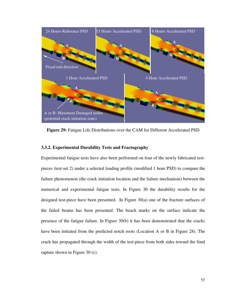
57

Figure 29: Fatigue Life Distributions over the CAM for Different Accelerated PSD

3.3.2. Experimental Durability Tests and Fractography

Experimental fatigue tests have also been performed on four of the newly fabricated test-

pieces (test-set 2) under a selected loading profile (modified 1 hour PSD) to compare the

failure phenomenon (the crack initiation location and the failure mechanism) between the

numerical and experimental fatigue tests. In Figure 30 the durability results for the

designed test-piece have been presented. In Figure 30(a) one of the fracture surfaces of

the failed beams has been presented. The beach marks on the surface indicate the

presence of the fatigue failure. In Figure 30(b) it has been demonstrated that the cracks

have been initiated from the predicted notch roots (Location A or B in Figure 28). The

crack has propagated through the width of the test-piece from both sides toward the final

rapture shown in Figure 30 (c).

24 Hours Reference PSD 15 Hours Accelerated PSD 8 Hours Accelerated PSD

1 Hour Accelerated PSD 4 Hour Accelerated PSD

A

Fixed end direction

A or B: Maximum Damaged nodes (potential crack initiation zone)

B

A

B

A

B

A

B

A

B

58

Figure 30: Failure of the Designed Test-Piece (Experimental)

(a)

(b)

(c)

Possible Crack Initiation Location

Possible Crack Initiation Location

A

B

Second semi-circular notch roots from the fixed end

Fixed end

B A

59

Figure 31(a): Fracture Surfaces of the Failed Test-Pieces

Fractographic examination has also been carried out to confirm the failure mechanism in

all of the fracture surfaces. These fracture surfaces (Sample 1, Sample 2 and Sample 3)

shown in Figure 31(a) have been examined under the optical electron microscope.

Optical microscope images of the fracture surfaces have been presented in the Figure

31(b) to show the features on the surfaces failed by fatigue testing. The beach marks in

every failure surface confirm the presence of fatigue as a consistent failure mechanism in

Sample 1

Sample 2 Sample 3

Area under optical microscope

Area under optical microscope

60

this case. The shiny surface of those figures refers to the region of stable crack growth

and the dull surface refers to the unstable crack growth towards final rupture.

Figure 31(b): Fracture Surfaces of the Failed Test-Pieces under the Optical Microscope

The cracks normal to the beach marks leading towards the notch roots (sample 2) indicate

these cracks initiate from the notch roots. Thus the failure mechanism (crack initiation

location and the failure type) has been verified by the experimental durability test and

fractography.

Sample 1 Sample 2

Sample 3

Dull Surface

Shiny Surface

Beach Marks

61

3.3.3. Effect of Plasticity and S-N Curve Slope in Durability Life

After the numerical durability analysis the experimental durability test has been

performed on the newly fabricated beam set 2. The partial test loading profile

corresponding to the 1-hour PSD has been used to carry out this test. However, the test

was not successful (failure time did not mach) due to the inaccuracy of the manufacturing

of the beam. Hence the 1-hour loading profile (Modified 1 hour loading profile) has been

modified to obtain desired dynamic response (natural frequencies, stresses and mode

shapes) in the preliminary tests.

To verify claimed inaccuracy of manufacturing, a sine sweep test with amplitude of 0.2 g

(peak-peak) in a frequency bandwidth of 3-65 Hz and 5-minute trial durability tests with

the 20-hour, 4-hour and 1-hour loading have been performed. The results from these

discussed tests have been compared with those from numerical analysis. In Table 7, the

natural frequency and the damping ratio have been compared between two test-sets of the

fabricated beams.

Table 8: Natural Frequencies and Damping Ratios for the First Two Bending Vibration

Modes for the Different Specimens

Test sets Natural Frequency of the 1st Mode

(Hz)

Damping Ratio of the

1st Mode (%)

Natural Frequency of the 3rd Mode

(Hz)

Damping Ratio of the 3rd Mode

(%)

Gain Ratio of the 1st

and 3rd Mode

1 7.114 0.2054 56.91 0.6857 3.190

2 6.856 0.3794 59.60 0.5546 3.120

Deviation 3.634% 84.76% 4.728% 19.11% 2.190

62

It is found that for the second set of beams the deviation from the expected value in the

natural frequency and damping ratio are 3.634% and 84.74% respectively. For the second

mode the deviation of these parameters has found as 19.11% and 2.190%. This deviation

of the damping ratio and the natural frequencies have significantly affected to the strain

distribution in the newly fabricated test-piece as well.

In Table 8, the experimental strain RMS from the location R_1, A_1 and A_2 shown in

Figure 16(a) have been compared with that of the FEA. The experimental strains have

been collected from the 5-minute trial durability test with the 20-hour, 4-hour and 1-hour

loading profiles. With this set of beams (set 2) the average deviation found for location

R_1 as 12.68%, A_1 as 13.01% and A_2 as 13.09% for different loading profiles which

is much higher than the previous set of beams.

Table 9: Comparison of Strains between the FE and the Experiment for Beam Set 2

Loading Profiles

Beam Set-Strain Gauges or Rosettes

Area Averaged

FE Strains (GH) RMS (1-Sigma)

Experimental

Strains(GH) RMS

Absolute Deviation in Strains (%)

20 hours PSD

2-A_1 492.8 580.9 17.88

2-A_2 473.0 575.3 21.56

2-R_1 512.5 617.9 20.50

04 hours PSD

2-A_1 643.8 630.8 2.014

2-A_2 618.0 624.6 1.061

2-R_1 669.5 670.9 0.217

Modified 01 hours

PSD

2-A_1 809.0 654.0 19.15

2-A_2 777.0 647.7 16.64

2-R_1 841.5 695.4 17.33

Thus the new fabricated beam is not supposed to fail within the prescribed time for which

it has been designed. Hence, the existing loading needs to be modified according to the

63

new test-piece. The average experimental durability life of the newly designed cantilever

beams (test set-2) which have been subjected to the modified 1-hour durability test has

been as 11.77 hours.

From Table 9, it has been found that the experimental fatigue life for the specimen is

11.77 hours which has been predicted as 0.706 hours for the modified 1 hour loading

using the standard S-N analysis. The possible reasons behind this deviation can be (1) the

involvement of plasticity, (2) inaccurate estimation of the slope of the S-N curve, b, in

the ‘test synthesis’ process. Hence, the effect of these two probable causes has been

investigated.

In the experiment, the strains have been found exceeding the elastic limit (~3855GH),

where the stress-strain relation is nonlinear which can underestimate the fatigue life. The

Von Mises, absolute maximum principal and maximum shear strain histories from

location R_1 and the sample bending strain histories from the location A_1 and A_2 have

been shown in Figure 32. From these strain histories, it has been observed that the

developed strains in these locations are exceeding the elastic limit of the considered

material. Therefore numerical strain life analyses using the experimental strains have

been used to accommodate the plasticity in the fatigue analysis and the fatigue life was

determined as 13.12 hours.

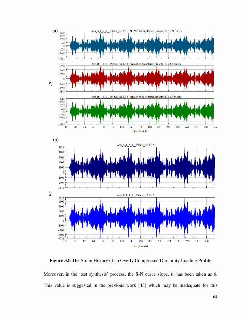
64

Figure 32: The Strain History of an Overly Compressed Durability Loading Profile

Moreover, in the ‘test synthesis’ process, the S-N curve slope, b, has been taken as 6.

This value is suggested in the previous work [43] which may be inadequate for this

(b))

(a))

GH

GH

65

specific material. Hence in this section the effect of the S-N curve slope has been

explored. To observe the effect of changing this parameter, b=5.5 [29] has been used with

the results shown in Table 10.

Table 10: Verification of the Synthesized AD Tests (b=5.5)

Parameters of AD Loading Profiles

AD Validation

Method

Expected Fatigue Life

of the Specimen

Fatigue Life Determined

Through FE based Fatigue Model

Absolute Percentage

(%) of Deviation

b=5.5 & TD=24 hours SRS & FDS 106.0 hours 106.0 Reference

b=5.5 & TD=20 hours SRS & FDS 88.33 hours 87.79 0.6113%

b=5.5 & TD=15 hours SRS & FDS 66.25 hours 72.32 8.3930%

b=5.5 & TD=12 hours SRS & FDS 53.00 hours 54.53 2.8870%

b=5.5 & TD=10 hours SRS & FDS 44.16 hours 46.43 4.4610%

b=5.5 & TD=08 hours SRS & FDS 35.33 hours 35.85 1.4720%

b=5.5 & TD=6 hours SRS & FDS 26.50 hours 27.02 1.9620%

b=5.5 & TD=4 hours SRS & FDS 17.66 hours 15.43 12.620%

b=5.5 & TD=2 hours SRS & FDS 8.833 hours

7.179 13.510%

It has been found from Table 10 that with the same AF, the expected and estimated

fatigue lives increase significantly as b decreases from 6 to 5.5. As discussed in the

Section 2.1, a lower value of b results in a lower magnitude of the generated PSD, which

allows a longer fatigue life, i.e., the inverse Basquin’s exponent b has a significant effect

on the generated durability testing loading profiles. Therefore using an improper S-N

curve exponent can be one of the causes for the discrepancy between the numerical and

experimental fatigue lives. As for generating a better AD testing profile, the effect of b

has been found crucial; so the material specific S-N curve can be used.

66

In contrary, Figure 33 has been plotted using the data set of Table 10 to show how the

estimated fatigue life deviates from the expected fatigue life for different time

compression ratios. The time compression (TC) ratio here is referred to the AF. The

standard deviation of the results found for different AF plotted in Figure 34 provides a

simple statistical evaluation of the estimated fatigue lives for b=5.5. So it is prominent

that the durability loading profiles are very effective for b=5.5 as well.

Figure 33: Comparison of the TC Ratio of Different AD Profiles

With the Theoretical One

Although the fatigue life increases with the decrease in b, the AF of the generated loading

profiles remains the same as the FLR, which indicates the ‘modified test tailoring

approach’ is equally efficient in different S-N curve exponent. Hence, the effectiveness

10 20 30 40 50 60 70 80 90 100 110 12010

20

30

40

50

60

70

80

90

100

110

120

Expected Fatigue Life of the Specimen, Hours

Est

imat

ed F

atig

ue L

ife

of t

he S

peci

men

, H

ours

Theoretical

TC ratio 13.75TC ratio 16.50

TC ratio 22

TC ratio 27.5

TC ratio 33

TC ratio 41.25TC ratio 55

TC ratio 82.5

67

of the AD profiles of different AF synthesized via ‘modified test tailoring approach’ has

been validated using a newly designed test-piece.

Figure 34: Deviation in the Determined Fatigue Life for Different TC Ratios

The following issues should also be considered into the ‘modified test tailoring

approach’:

(1) The ‘test tailoring approach’ is based on linear SDOF system which is limited to

the elastic limit for the material.

(2) If the generic b is used to synthesis the AD loading profiles, it is necessary to

check the developed stress level (plastic/elastic) in the test-piece for the

synthesized AD loads.

(3) To account the plasticity in the fatigue analysis the strain life method should be

adopted to predict the structural life with over-compressed AD loading profile.

0 25 50 75 100 125 150 17510

20

30

40

50

60

70

80

90

100

110

Time Compression (TC) Ratio

Fat

igue

Lif

e of

the

Spe

cim

en,

Hou

rs

68

An over -compressed loading profile has an ERS higher than the SRS of the field

test and has the FDS same as the FDS of the same as the field test. Though

generation of this kind of loading profile is not encouraged in the ‘test tailoring

approach’, strain life analysis can be used as a remedy.

69

Chapter 4

Conclusions and Future Works

A computer-aided AD test has been performed to validate the ‘modified test tailoring

approach’ of generating highly AD loading profiles for ground vehicle components. This

approach has been previously proposed in [43]-[44] due to the limitations of testing

implementation and the requirement of high AF in the durability tests of heavy ground

vehicle components. In the modified approach, the full period of accelerated PSD can be

represented by an equivalent 60s time series multiples, keeping the same amount of

damage. This new modified approach needs to be validated. Hence in this work, the 330-

hour field test has been accelerated up to a 1-hour durability test using the modified

approach and the corresponding fatigue analysis has been performed on a newly designed

test-piece to verify those AD loading profiles, hence the ‘partial test approach’.

In this work, the test-piece has been designed via a conjugative approach involving FEA

and fatigue analysis for a specific 24 hours of durability life. To justify the design, it has

been satisfactorily tested against the experiment. Good agreements have been found

between the numerical results from the CAM and the experimental result of the test-

piece. Hence the developed CAM properly represents the physical system used in the

experiment.

70

Numerical fatigue tests have been performed on the verified CAM using the generated

AD loading profiles and a sound agreement has also been found on the estimated and the

expected fatigue lives. The effectiveness of the synthesized AD loading profiles has also

been observed almost insensitive to the S-N curve; hence the modified approach can be

used for a wide range of materials. From the simulation results, the estimated crack

initiation locations are the same for different AD loading profiles. In addition, these

initiation locations have been found identical in the experiment and the simulations.

Moreover, fractography shows the beach marks on the failure surfaces which indicate the

presence of fatigue failure of the specimen. Although in this study the experimental and

the numerical fatigue lives have not matched for the designed test-piece, the failure

mechanism has been found to be consistent between the experimental and numerical

analyses. The probable reasons behind the discrepancy in the fatigue lives under 1-hour

loading profile has been investigated and outlined in the previous Section 3.3. Thus, the

AD profiles synthesized based on the modified approach have also successfully passed

the computer-aided fatigue tests.

The modified approach is very promising to produce the driving files for the test rig to

perform highly AD tests of the ground vehicle components. As future work, aaccelerated

labs tests can be performed with the generated durability loading profiles validate the

durability life of the test-piece. Furthermore, the use of the ‘Transmission Electron

Microscopy' to examine the effect of local plasticity can be a very good addition to the

current work. Importantly, caution should also be taken to the fact that the modified

approach is valid up to the elastic limit of the material when accelerating the field test

with high an AF.

71

References

[1]. Pennsylvania Transportation Institute – Vehicle System and Safety Group. (2007,

Nov. “Bus Research and Testing Facility (“Test Track”) [Online] Available:

http://www.vss.psu.edu/BTRC/btrc_test_track_htm.

[2]. Xu Ke, Development of Vibration Loading Profiles for Accelerated Durability

Tests of Ground Vehicles, MSc thesis, University of Manitoba, (2011).

[3]. K. Dressler, M. Speckert, and G. Bitsch. “Virtual durability test rigs for automotive

engineering”, Vehicle System Dynamics. vol. 47 (4) April 2009, 387-401.

[4]. Steve S., “An introduction to Mutli-Axes Simulation Tables (MAST)”, Slides from

WESTEST, 2010.

[5]. Nelson, W., 1990, Accelerated Testing, Statistical Models, Test Plans and Data

Analyses, John Wiley & Sons, New York.

[6]. Caruso H and Dasgupta A.," A Fundamental Overview of Accelerated Testing

Analytical Models", Reliability and Maintainability Symposium (RAMS)

Proceedings, IEEE, 1998, pp. 389 – 393.

[7]. Meeker, W.Q. & Escobar, L.A. (1993). A Review of Recent Research and Current

Issues in Accelerated Testing, International Statistical Review 61, 1, pp. 147-168.

[8]. Ashmore C., Piersol A. G., Witte J. J., 1992, “Accelerated Service Life Testing of

Automotive Vehicles in a Test Course”, Vehicle Systems Dynamics , Vol. 21,

pp.89–108.

[9]. Abdullah S, Nizwan C K E, Nauwi M Z, 2009, A Study of Fatigue Data Editing

Using the Short-Time Fourier Transform (STFT), American Journal of Applied

Science 6(4): 565-575.

[10]. Kadhim N A, Abdullah S, Ariffin A K. Effect of the fatigue data editing technique

associated with finite element analysis on the component fatigue design period.

Materials and Design, 2011: 32 1020-1030.

72

[11]. Stephens et. al., Fatigue Damage editing for accelerated durability testing using

strain range and SWT parameter criteria, Int. J. of Fatigue Vol. 19, Nos 8-9, pp.

599606, 1997.

[12]. Yay, K., Ereke, I. M., Bilir, M., Cataltepe, V. , 2009, Fatigue strength of an urban

type midi bus vehicle chassis by using FEM analysis and accelerated fatigue life

test, Society of Automotive Engineers World Congress, ISSN 0148-7191, Detroit,

USA.

[13]. Ziong J.J., Shenoi R.A., A load history generation approach for full-scale

accelerated fatigue tests, Engineering Fracture Mechanics 75 (2008) 3226–3243.

[14]. Lin, K-Y, Hwang, J-W and Chang, J-M, Accelerated durability assessment of motor

cycle components in real life simulation testing, Proc. IMechE Vol. 224 Part D: J.

Automobile Engineering, 2009.

[15]. Abdullah, S, Giacomin, J A, and Yates, J R, A mission synthesis algorithm for

fatigue damage analysis, Proc. IMechE Vol. 218 Part D: J. Automobile

Engineering, 2004.

[16]. Chinnaraj K , Sathya P M, Lakshmana R C. Dynamic Response Analysis of a

Heavy Commercial Vehicle Subjected to Extreme Road Operating Conditions.

Journal of Physics: Conference Series 181 (2009) 012070, doi:10.1088/1742-

6596/181/1/012070.

[17]. Haiba M., Barton D.C., Brooks P.C. and Levesley M.C., Review of life assessment

techniques applied to dynamically loaded automotive components, Computers and

Structures 80 (2002) 481–494.

[18]. N.W.M. Bishop, The use of frequency domain parameters to predict structural

fatigue, PhD thesis, Warwick University, (1988).

[19]. Jhung D.H. and Bae S.I., Automotive Component Fatigue Life Estimation by

Frequency Domain Approach, Key Engineering Materials, Vols. 297-300 (2005),

pp. 1776-1786.

[20]. N.W.M.Bishop, Vibration Fatigue Analysis in the Finite Element Environment,

XVI ENCUENTRO DEL GRUPO ESPAÑOL DE FRACTURA, (1999).

73

[21]. Halfpenny A., A Frequency Domain Approach for Fatigue Life Estimation from

Finite Element Analysis, Key Engineering Materials, Vols. 167-168 (1999), pp.

401-410.

[22]. A. Al-Yafawi, S. Patil, D. Yu, S. Park, J. Pitarresi, Random Vibration Test for

Electronic Assemblies Fatigue Life Estimation, Thermal and Thermomechanical

Phenomena in Electronic System (ITherm), IEEE, 2010, pp. 1-7.

[23]. S. Patil, D. Yu, S. Park, S. Chung, Finite Element Based Fatigue Life Prediction for

Electronic Components under Random Vibration Loading, Electronic Components

and Technology Conference (ECTC), IEEE, 2010, pp. 188-193.

[24]. Ma C.H., Study of Acoustic Fatigue Life Estimation for Composite Structure Based

on Power Spectral Density, Materials Research Innovations, Vols. 15 (2011), pp.

118-121.

[25]. Li R. S., 2001, ‘‘A Methodology for Fatigue Prediction of Electronic Components

under Random Vibration Load,’’ ASME J. Electron. Packag. 123(4), Dec., pp.

394–400.

[26]. Hyun D.H., Automotive Component Fatigue Life Estimation by Frequency Domain

Approach, Key Engineering Materials, Vols. 297-300(2005), pp. 1776-1783.

[27]. Moon S-I, Chao I-J and Youn D, Fatigue Life Evaluation of Mechanical

Components Using Vibration Fatigue Analysis Technique, Journal of Mechanical

Science and Technology 25 (3) (2011) 631-637.

[28]. C-J. Kin, Y. J. Kang, B-H. Lee, Experimental spectral damage prediction of a linear

elastic system using acceleration response, Mechanical Systems and Signal

Processing 25 (2011) 2538–2548.

[29]. Pothula A, Gupta A and Kathawate Guru R (2011) Fatigue failure in random

vibration and accelerated testing, Journal of vibration and control 0(0), 1-8.

[30]. Pace, L., Jayat, F., Konieczny, R., Forster, M. et al., "Accelerated Durability Test

for Metallic Substrates Tailored for Motorcycle Application," SAE Technical

Paper 2011-32-0512, 2011, doi:10.4271/2011-32-0512.

[31]. Wala MKBG and Gupta, A, “Accelerated testing and Damping”, Proceedings of

International Modal Analysis Conference XXVII: Conference & Exposition on

Structural Dynamics, 2009.

74

[32]. Nagulapalli VK, Gupta, A, and Fan S. “Estimation of Fatigue Life of Aluminum

Beams subjected to Random Vibration”, Proceedings of International Modal

Analysis Conference XXV, 2007.

[33]. J. Pulido, Practical Reliability of Structure under Road Loading, Reliability and

Maintainability Symposium (RAMS) Proceedings, IEEE, 2011, pp. 1-7.

[34]. Allegri G, Zhang X., On the inverse power laws for accelerated random fatigue

testing, International Journal of Fatigue, 30 (2008): 967-977.

[35]. Sun FQ, Li XY, Zhang ZR and Jiang TM, 2010, Step-stress Accelerated Random

Vibration Life Testing, Advanced Material Research, Vol. 118-120, pp.606–610.

[36]. Lee Y-L, Polehna D and Kang H-T, 2010, “Fatigue Damage Severity Calculation

for Vibration Test”, Journal of Testing and Evaluation, Vol. 38(6), pp.1–10.

[37]. Halfpenny A. (2006). Mission Profiling and Test Synthesis based on fatigue damage

spectrum. Ref. FT342, 9th Int. Fatigue Cong. Atlanta, USA. Elsevier, Oxford, UK.

Available: www.hbm.com/ncode.

[38]. Pompetzki, M., Dabel B,, Lin X., (2010), Advancement in Automotive Durability

Process, Structural Durability and Health Monitoring, Vol. 5, No. 2, pp.69–76.

[39]. Halfpenny A and Kihm F. Environmental Accelerated Testing. Use of Virtual test

to extend physical Approach, White Paper (2008). Available:

www.hbm.com/ncode.

[40]. Jung D-H. Reliability achievement of the driving systems parts through

development of vibration-fatigue evaluation method. Engineering Procedia 10

(2011) 1906-1916.

[41]. Özsoy S, Celik M, Kadioglu F S. An accelerated life test approach for aerospace

structural components, Eng Fail Anal 2008; 15(7): 956-957.

[42]. M. Aykan, M. Celik , Vibration fatigue analysis and multi-axial effect in testing of

aerospace structures, Mechanical Systems and Signal Processing 23(2009) 897-

907.

[43]. Xu K., Wu Y. and Wu C. Q., 2011 Development of Vibration Loading Profiles for

Accelerated Durability Tests of Ground Vehicles, 4th Annual Dynamic Systems

and Control Conference, Arlington, VA, USA.

75

[44]. S. Cull, C. Yang, and C. Wu, “Generation and verification of accelerated durability

tests”, Department of Mechanical and Manufacturing Engineering, University of

Manitoba, Internal Report, 2010.

[45]. GlyphWorks Theory [Electronic], Available with nCode GlyphWorks software,

nCode, 2010.

[46]. ANSYS13.0 Software ANSYS Inc., Canonsburg, PA, USA.

[47]. DesignLife Worked-out Examples [Electronic], Available with nCode GlyphWorks

software, nCode, 2010.

[48]. Piersol A. G., “ACCELERATED VIBRATION TESTING- proceed with caution,”

Tustin Training News, January 1993. Available at: http://www.ttiedu.com.

[49]. NATO AECTP 200 (2003). Validation of mechanical environmental test methods

and severities. NATO AECTP 200, Ed. 3, Section 2410. Final Draft Sept 2003.

[50]. Wannenburg, J. and Heyns, P.S. (2010) ‘An overview of numerical methodologies

for durability assessment of vehicle and transport structures’, Int. J. Vehicle

Systems Modeling and Testing, Vol. 5, No. 1, pp.72–101.

[51]. Zalaznik A and Nagode M. Frequency Based Fatigue Analysis and Temperature

Effect. Materials and Design 32 (2011) 4794–4802.

[52]. Palsma E.S. and Vidal F.A.C., (2002), Fatigue Damage Analysis of on Body Shell

Of A Passenger Vehicle, Journal of Materials Engineering and Performance, Vol.

11, No. 4, pp.450-460.

[53]. J. Gilbert Kaufman, 2008, “Properties of Aluminum Alloys-Fatigue data and the

effects of temperature, Product Form and Processing”, ASM international, ISBN-

10:0-871170-839-7.

[54]. Multi-axial Fatigue Theory, MSC software [online], Available at: http: // www.

mscsoftware.com/training_videos/patran/Reverb_help/index.html#page/Fatigue%2

0Users%20Guide/fat_mulitaxial.07.5.html.

[55]. P. M. Hall, On Using Strain Gauges in Electronic Assemblies When Temperature Is

Not Constant, IEEE Transactions On Components, Hybrids And Manufacturing

Technology, Vol .Chmt-9,No.4,December 1986.

[56]. Han S. and Chung J.W., A, “Retrieving Displacement Signal from Measured

Acceleration Signal”, Proceedings of International Modal Analysis Conference

76

XX: Conference & Exposition on Structural Dynamics, 2002.

[57]. Shafiullah, A.K.M., Wu, C.Q., 2012, “Validation of Loading Profiles for

Accelerated Durability Testing of Ground Vehicle Components”, Proceedings of

CSME. (Submitted).

[58]. Heiber G., “Test Time Exaggeration Factor,” Tustin Training News, 1994.

Available: http://www.ttiedu.com.

[59]. Paulus M. and Doughty K. (2010) ‘Effect of Resonant Frequency Shifting on Time

to Failure of a Cantilevered Beam under Vibration , Journal of IEST, Vol. 53, No.

1, pp.59–68.

[69]. Petracconi et. al., Fatigue life simulation of a rear tow hook assembly of a passenger

car, Engineering Failure Analysis 17 (2010) 455–463.

[61]. Oman S, Fazdiga M, Nagode M. Estimation of air-spring life based on accelerated

experiments. Materials and Design, 2011: 32 1020-1030.

[62]. “Theoretical and Experimental Researches Using Accelerated Life Testing in

Aerospace”, International Journal for Engineering and Information Sciences ,Vol.

4, No. 2, pp. 117–122 (2009).

[63]. Brown G.W. and Ikegami R.," The Fatigue of Aluminium Alloys Subjected to

Random Loading", Experimental Mechanics. 1970, pp. 321-327.

[64]. D. Benasciutti, R. Tovo, “Spectral methods for lifetime prediction under wide-band

stationary random processes”, International Journal of Fatigue, vol.27, pp. 867-877,

2005.

[65]. S. Srikantan, S. Yerrapalli, H. Keshtkar, “Durability design process for truck body

structure”, International Journal of Vehicle Design, vol.23, pp. 94-108, 2000.

[66]. Specification Development using ERS and FDS, Available at: http: //

christian.lalanne. free.fr/Home/Home_ E.htm, 2009.

[67]. Western Canada testing Inc. (Feb, 2008). “WESTEST MAST Table” [Online].

Available: http://www.westest.ca /mast.htm [August 16, 2009].

77

Appendices

Appendix A- Details of the all Considered Test-Pieces and their

Comparison with the Selected One

Three other test-pieces has also been modeled and fabricated to verify the adopted

numerical method in this work. These three models have different fatigue life than 24

hours under the reference loading. The fatigue lives of all the four different

models/specimens are presented in Table 1A.

Table 1A: Fatigue Lives of Different Test-Pieces under the 24 Hours Loading

Test Duration

Fatigue Lives in Hours

Specimen 1 (selected)

Specimen 2 Specimen 3 Specimen 4

24 hour 23.80 5.436 131.2 9385

Other than the fatigue life, the criterions presented in Section 2.2 have been maintained

mentioned, while modeling those specimens. The dynamic features of all of the 4

specimens have been compared in this section. Among the specimens the selected one

shows the ‘best fit’ with the experiments.

Table 2A shows that all of the considered specimens have two bending modes in the

frequency range of 0-60 Hz. The lateral modes have not been extracted from the

experiment as only the vertical excitation has been applied. Table 3A demonstrates the

dominancy of the bending mode in the considered frequency range (0-60 Hz). It is

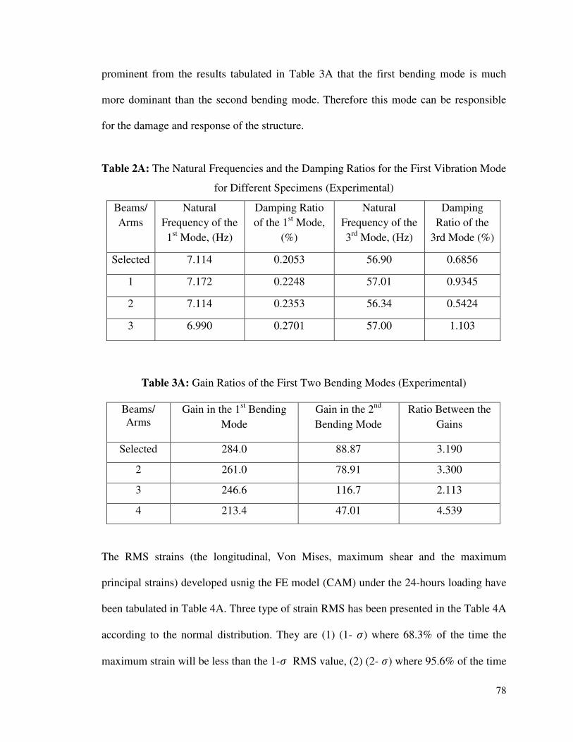
78

prominent from the results tabulated in Table 3A that the first bending mode is much

more dominant than the second bending mode. Therefore this mode can be responsible

for the damage and response of the structure.

Table 2A: The Natural Frequencies and the Damping Ratios for the First Vibration Mode

for Different Specimens (Experimental)

Beams/ Arms

Natural Frequency of the 1st Mode, (Hz)

Damping Ratio of the 1st Mode,

(%)

Natural Frequency of the 3rd Mode, (Hz)

Damping Ratio of the

3rd Mode (%)

Selected 7.114 0.2053 56.90 0.6856

1 7.172 0.2248 57.01 0.9345

2 7.114 0.2353 56.34 0.5424

3 6.990 0.2701 57.00 1.103

Table 3A: Gain Ratios of the First Two Bending Modes (Experimental)

Beams/ Arms

Gain in the 1st Bending Mode

Gain in the 2nd Bending Mode

Ratio Between the Gains

Selected 284.0 88.87 3.190

2 261.0 78.91 3.300

3 246.6 116.7 2.113

4 213.4 47.01 4.539

The RMS strains (the longitudinal, Von Mises, maximum shear and the maximum

principal strains) developed usnig the FE model (CAM) under the 24-hours loading have

been tabulated in Table 4A. Three type of strain RMS has been presented in the Table 4A

according to the normal distribution. They are (1) (1- ?) where 68.3% of the time the

maximum strain will be less than the 1-? RMS value, (2) (2- ?) where 95.6% of the time

79

the maximum strain will be less than the 2-? RMS value and (3) (3- ?) where 99.7% of

the time the maximum strain will be less than the 3-? RMS value.

Table 4A: Strains Developed in the 24 Hours Durability Test in the FE Models

Beams/ Arms/

Specimens

Type of the

Strain Result

Maximum Strain in the X direction (Longitudinal axis

of the beam) (µE )

Maximum Von Mises

Strain

(µE )

Maximum Shear Strain (XZ Plane)

(µE )

Maximum Principal

Strain

(µE )

Selected (Set 1)

(1-?) 802.3 814.6 769.5 835.6

(2-?) 1604 1629 1539 1707

(3-?) 2407 2443 2308 2506

1 (1-?) 756.4 756.1 623.3 756.4

(2-?) 1512 1512 1246 1512

(3-?) 2269 2268 1870 2269

2 (1-?) 741.7 741.8 609.7 743.2

(2-?) 1483 1483 1219 1486

(3-?) 2225 2225 1818 2230

3 (1-?) 710.4 709.1 590.6 712.9

(2-?) 1420 1418 1181 1426

(3-?) 2131 2127 1772 2138

Table 5A shows the comparison of the natural frequencies between the experiment and

the FEA results for considered specimens. First four modes have been taken for the

comparison. The lateral vibration mode (second mode) has not been compared as only

vertical excitation has been considered. From the results, for the first vibration mode the

least deviation has been observed in ‘Specimen 2’ as 1.723% and the most one as 2.702%

in specimen 3. Overall the maximum deviation in the natural frequency has been found in

‘Specimen 2’ as 5.090% in the fourth mode. The maximum deviations in the natural

80

frequencies (of the specimens) between the FEA and experimental results have also been

presented in Figure 1A with bar diagrams. Through this figure a comparison of the ‘good

of fit’ of the specimen’s analytical (FEA) natural frequency with the experiments have

been demonstrated.

Table 5A: Comparison of the Natural Frequencies between the FE and the Experimental model

Beams/

Arms/

Specimens

Vibration Modes Experimental Natural

Frequencies (Hz)

Analytical Natural

Frequencies (Hz)

Absolute Percentage (%)

of Deviation

Selected First (bending) 7.114 7.273 2.163

Second (transverse) N/A 33.82 ------------

Third (bending) 56.91 59.66 4.616

Fourth (bending) 165.8 174.7 5.090

1 First (bending) 7.171 7.297 1.723

Second (transverse) N/A 35.441 ---------

Third (bending) 57.01 59.57 4.288

Fourth (bending) 167.40 175.5 4.654

2 First (bending) 7.114 7.308 2.661

Second (transverse) N/A 34.718 -----------

Third (bending) 56.34 59.13 4.728

Fourth (bending) 164.8 173.4 4.941

3 First (bending) 6.989 7.184 2.702

Second (transverse) N/A 32.987 ---------

Third (bending) 57.00 59.82 4.723

Fourth (bending) 166.6 175.4 5.056

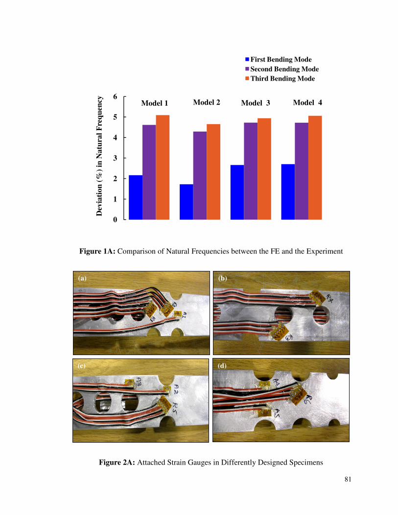
81

Figure 1A: Comparison of Natural Frequencies between the FE and the Experiment

Figure 2A: Attached Strain Gauges in Differently Designed Specimens

0

1

2

3

4

5

6D

evia

tion

(%

) in

Natu

ral

Fre

qu

ency

First Bending Mode

Second Bending Mode

Third Bending Mode

Model 1 Model 2 Model 3 Model 4

(a) (b)

(c) (d)

82

According to this ‘good of fit’ the specimens can be arranged in the following order:

Specimen 2, Specimen 1, Specimen 3 and Specimen 4. Table 6A presents a comparison

of maximum Von Mises strain results at different locations of the considered specimens

determined via FEA and experiments. In these locations, presented in Figure 2A, the

strain gauges have been attached to the beams to collect the experimental strains. In this

figure R1, R2, R3, R4, R5, R6 are strain rosettes and A1, A2, A3, A4 and A5 are the

axial strain gauges.

Table 6A: Comparison of Strains between the FEA and the Experiment

Strain Gauges/ Rosettes

Attached with the Arm

No

Area Averaged FE Strains (µE)

Experimental Strains (µE)

Absolute Deviation in Strains (%)

A1 Selected 1416 1454 2.610

R1 Selected 984.0 990.5 0.660

R2 Selected 1266 1271 0.390

R3 1 1639 1880 12.79

R4 1 1500 1725 13.04

A2 2 1635 1695 3.540

A3 2 1318 1317 0.114

R5 2 1359 1290 5.349

A4 3 1624 1583 2.620

A5 3 1336 1305 2.414

R6 3 1329 1272 4.481

The strains have been collected from 24-hours trial durability test. From this table, the

least average (of location A1, R1 and R2) deviation in the strain results has been found

as 1.22% in the selected specimen and the maximum average (of R1 and R2) deviation is

83

listed as 12.92% in specimen 2. The average strain deviation is 3% (considering location

A2, R3 and R5) and 3.17% (considering location A4, A5 and R6) in specimen 3 and

specimen 4respectively.

In Figure 3A, the average deviations (%) in the maximum Von Mises strain results for

the considered specimens have been presented via bar diagrams. From Figure 3A it is

prominent that the experimental strain in specimen 1 is the least deviated from the FEA

with the applied assumptions.

Figure 3A: Comparison of the Strain Results between the FE and the Experiment

Table 7A presents the strain ratio of two different location of the same specimen

determined from both FEA and experiments. In this case the deviations of strain ratios

have been found significantly lower, which further indicates that the FE model is good

enough to predict the strains. The maximum deviation in this ratio between the FEA and

0

2

4

6

8

10

12

14

Dev

iati

on

(%

) in

Str

ain

Res

ult

s

Geometric model 1

Geometric model 2

Geometric model 3

Geometric model 4

84

experiment has been found as 2.070% among all the considered pairs of gauges presented

in Table 7A.

Table 7A: Comparison of Strain Distributions between the FE and the Experiment

Strain Gauges/ Positions

Ratios of Strains from FEA

Ratios of strain from Experiments

Absolute Deviation

A5, A4 1.216 1.213 0.2467 %

A4, R6 1.222 1.244 1.807 %

R2, R1 1.286 1.283 0.272 %

A1, R1 1.439 1.469 2.070 %

R3, R4 1.093 1.089 0.283 %

A2, A3 1.240 1.287 1.240 %

85

Appendix B- Other Fatigue Results

The fatigue life using the experimental strains collected from different locations

presented in Figure 2A has been demonstrated in the Table 8A.

Table 8A: Fatigue Lives in Different Locations of the Specimens Based on Experiments

Beams/ Arms/

Specimens

Locations Approaches Fatigue Lives

(hours)

1 A1 SN Method with Goodman correction 208.0

1 R1 SN Method with Goodman correction 7613.0

1 R2 SN Method with Goodman correction 773.6

2 R3 SN Method with Goodman correction 58.89

2 R4 SN Method with Goodman correction 26.60

3 A2 SN Method with Goodman correction 63.00

3 A3 SN Method with Goodman correction 680.9

3 R5 SN Method with Goodman correction 736.9

4 A4 SN Method with Goodman correction 153.2

4 A5 SN Method with Goodman correction 931.1

4 R6 SN Method with Goodman correction 1145

In this case, the fatigue lives have been determined in the time domain using the stress

life (S-N) technique. Goodman criterion has been used to correct the mean stress effect.

These results can be used with the results from Table 5A to deduce a relationship

between the strain RMS value and the expected fatigue life. This relationship can be used

86

as a preliminary tool to find out the fatigue life of critical locations based on the

developed stress.

Furthermore, in the frequency-domain-based S-N method for fatigue life estimation

depends on the different of cycle counting algorithms. It has previously been found that

Dirlik algorithm in the frequency-domain-based techniques has the best match with the

‘rainflow cycle counting algorithm’ in the time based domain techniques. In this case,

effect of other different cycle counting algorithms like Narrowband, Steinberg and

Lalanne on the fatigue life of the specimens have also been explored. It has been found

that the Narrowband algorithm yields a conservative value of fatigue life and Lalanne

algorithm overestimate the fatigue life than the other two algorithms. In this work,

Specimen 1 has been designed for 23.8 hours under the reference 24 hours AD loading

profile using Dirlik’s algorithm. Table 9A represents the fatigue life of four selected

specimens using different cycle counting algorithms in frequency domain.

Table 9A: Estimated Fatigue Life of the Four Selected Specimens Using Different Cycle

Counting Algorithms in the Frequency Domain

Loading Duration

Cycle Counting Algorithm

Fatigue Life in Hours

Specimen 1 (Selected)

Specimen 2 Specimen 3 Specimen 4

24 hours

Dirlik 23.80 5.436 131.2 9385

Narrowband 8.416 5.424 130.7 2482

Steinberg 10.30 6.979 159.4 3206

Lalanne 38.48 5.428 130.9 1.223 x104

20 hours

Dirlik 19.46 4.044 105.5 6548

Narrowband 7.037 4.035 105.1 1659

Steinberg 8.630 5.479 128.2 2204

87

Table 9A (Cond.) Loading Duration

Cycle Counting Algorithm

Fatigue Life in Hours

Specimen 1 (Selected)

Specimen 2

Specimen 3 Specimen 4

20 hours Lannane 31.50 4.038 105.2 7827

15 hours

Dirlik 15.24 2.331 67.26 5606

Narrowband 7.876 2.326 67.06 1483

Steinberg 9.740 3.760 81.98 1970

Lannane 25.17 2.327 67.12 5573

10 hours

Dirlik 9.419 0.880 31.18 2484

Narrowband 2.927 0.878 31.07 593.4

Steinberg 3.744 1.771 38.41 708.1

Lannane 10.92 0.878 31.11 2468

8 hours

Dirlik 8.391 0.721 26.66 2155

Narrowband 2.055 0.719 26.57 472.9

Steinberg 2.658 1.480 32.98 564.4

Lannane 8.540 0.720 26.60 2142

4 hours

Dirlik 4.091 0.421 17.26 1468

Narrowband 1.258 0.420 17.20 319.2

Steinberg 1.695 0.986 21.72 384.4

Lannane 5.336 0.421 17.22 1497

2 hours

Dirlik 1.901 0.223 10.63 821.4

Narrowband 0.709 0.223 10.59 193.1

Steinberg 1.023 0.597 13.80 232.2

Lannane 3.098 0.222 10.60 915.4

1 hours

Dirlik 1.045 0.062 3.557 352.6

Narrowband 0.244 0.062 3.543 77.50

Steinberg 0.442 0.148 5.298 94.16

Lalanne 1.017 0.062 3.547 350.3

88

Appendix C- Miscellaneous Findings While Generating the AD Test

Figure 4A presents the ERS of the partial tests of different duration. These partial tests

has been synthesized using inverse Basquin’s exponent, b=6. It has been observed that

the ERS of the synthesized profiles exceeds the SRS of the field test in a good manner

when the duration of the partial tests is 10 hours or less. All the synthesized loading

profiles are equivalent to 330 hours of field test.

Figure 4A: Response Spectra of Different AD Tests for Constant FDS (b=6)

0 10 20 30 40 50 600

0.5

1

1.5

2

2.5

3

3.5

Frequency, Hz

Acc

eler

atio

n, g

8 hour ERS

10 hour ERS

15 hour ERS24 hour ERS

Field Test SRS

89

Therefore it is necessary to conclude that using suggested b=6 by Xu [2], the accelerated

loading profiles should not be generated for 12 hours or less. Hence to generate loading

profiles up to 1 hour a different S-N curve slope, b=5.5 has been used in this work.

There are different algorithms to calculate the FDS from the input acceleration data. The

Rayleigh and Lalanne are two of these algorithms which produce the FDS with slightly

different damage content. It has been observed from the comparison of Figure 5A and

Figure 14 that for the Lalanne algorithm, FDS of the partial tests fit better with the FDS

of the field test than the Rayleigh algorithm.

Figure 5A: Damage Spectra of Different AD Tests for Constant FDS (b=6)

AD loading profiles also can also be synthesised keeping the ERS constant. In this case

the FDS of the AD loading profiles will vary with the change of the duration of the

loading profiles. Figure 6A presents the ERS of different AD profiles when SRS of the

0 10 20 30 40 50 6010

-20

10-15

10-10

10-5

100

105

Frequency, Hz

Dam

age

1 hour FDS

6 hour FDS

12 hour FDS24 hour FDS

Field Test FDS

Rel

ativ

e D

amag

e S

pect

rum

Lev

el

90

field test has been taken as the input to the ‘test synthesis’ process. This technique

enables us to generate the AD profiles with less duration as the ERS of loading profile is

insensitive with the attained AF. However, as the FDS does change in this technique,

there is a good chance of the alteration of failure mechanism in this case. Hence

practically this technique should not be practised.

Figure 7A shows the equivalent FDS of the different AD loading profile which has been

synthesized keeping the ERS constant. This figure demonstrates that equivalent FDS of

the AD loading profile changes when the duration of the AD test changes for a constant

ERS. Thus in this approach the response of the system can be controlled by sacrificing

the damage content which is not recommended.

Figure 6A: Response Spectra for Different AD Tests (Full) for Constant ERS (b=6)

0 10 20 30 40 50 600

0.5

1

1.5

2

2.5

3

3.5

Frequency, Hz

Acc

eler

atio

n, g

1 hour ERS

8 hour ERS

24 hour ERS48 hour ERS

Field Test SRS

91

Figure 7A: FDS for Different AD Tests (Full) For Constant ERS (b=6)

0 10 20 30 40 50 6010

-25

10-20

10-15

10-10

10-5

100

Frequency, Hz

Dam

age

8 hour FDS

10 hour FDS15 hour FDS

24 hour FDS

Rel

ativ

e D

amag

e S

pect

rum

Lev

el