development of a 2-d 2-group neutron noise simulator

Development of a 2-D 2-group neutronnoise simulator

C. Demaziere*

Chalmers University of Technology, Department of Reactor Physics, SE-412 96 Goteborg, Sweden

Received 10 May 2003; accepted 27 August 2003

Abstract

In this paper, the development of a so-called neutron noise simulator is reported. Thissimulator calculates both the direct and the adjoint reactor transfer function between a stat-ionary noise source and its induced neutron noise for any 2-dimensional heterogeneous crit-

ical system. The main advantage of this neutron noise simulator is that any realistic core canbe modelled, since the simulator is designed to rely on a set of material constants corres-ponding to the actual reactor operating conditions. The calculations are performed in the

2-group diffusion approximation and in the frequency domain. The spatial discretisation iscarried out with respect to the finite difference scheme. The noise source, expressed as an‘‘absorber of variable strength’’ type, is defined directly from the fluctuations of the macroscopic

cross-sections and can be spatially distributed over the core or concentrated in a few discretenodes. If the noise source is a point-source, the simulator actually estimates the 2-dimensional2-group discretised Green’s function of the system. From the calculated Green’s function, theneutron noise induced by a ‘‘vibrating absorber’’ type of noise source can also be determined.

Different benchmark cases show that this neutron noise simulator works satisfactorily.# 2003 Elsevier Ltd. All rights reserved.

1. Introduction

It is well known that the neutron noise, i.e. the difference between the time-dependent neutron flux and its time-averaged value, assuming that all the processesare stationary and ergodic in time, allows the determination of many interestingfeatures of a reactor. The neutron noise can be used either for diagnostic purposes,

Annals of Nuclear Energy 31 (2004) 647–680

www.elsevier.com/locate/anucene

0306-4549/$ - see front matter # 2003 Elsevier Ltd. All rights reserved.

doi:10.1016/j.anucene.2003.08.007

* Tel.: +46-31-772-3082; fax: +46-31-772-3079.

E-mail address: [email protected] (C. Demaziere).

http://www.sciencedirect.com



http://www.elsevier.com/locate/anucene/a4.3d

mailto:[email protected]

when an abnormal situation is suspected, or for estimating a dynamical core para-meter, whereas the reactor is at steady-state conditions. Many examples can befound in the literature (Thie, 1963; Thie, 1981; Uhrig, 1970; Williams, 1974). Forthe former, it is now common practice to determine any flow blockage by esti-mating the flow velocity in the corresponding fuel channel. The cross-correlationbetween two neutron detectors can be used for that purpose. But the neutron noisecan be utilized for other diagnostics tasks, such as the estimation of core barrelvibrations, or the localisation of a noise source such as an unseated fuel assembly.For the latter category, namely the determination of global dynamical core para-meters, the Decay Ratio in Boiling Water Reactors (BWRs) (D’Auria et al., 1997)and the Moderator Temperature Coefficient of reactivity in Pressurised WaterReactors (PWRs) (Demaziere and Pazsit, 2003b) are probably the two most sig-nificant applications.

Consequently, the calculation of the dynamic reactor transfer function, i.e. theneutron noise induced by a given noise source, is of prime importance. Althoughmany commercial codes for static calculations are available, there is no dedicatedcode, to our knowledge, that is able to calculate the dynamic reactor transfer func-tion. Even if time-dependent codes are used to estimate the Decay Ratio forinstance, the neutron noise has not been given enough attention so far. Severalresearch groups demonstrated that the calculation of the dynamic reactor transferfunction was possible mainly by modifying existing static core simulators, but nocode specifically dedicated to the calculation of the neutron noise in power reactorswas ever developed. As a matter of fact, only simplified dynamic reactor transferfunctions have been estimated in the literature, for instance in case of homogeneousreactors, or reactors assumed to be constituted of a few homogeneous regions.Williams (1967) and Analytis (1982) were probably the first authors contributing themost to the calculation of the reactor noise in heterogeneous systems. In thesepapers, the source-sink method of Horning, Feinberg, and Galanin was used fortreating the neutron noise of point-like fuel pins surrounded by a moderator. Due tothe complexity of this method, only infinite lattice problems could be investigated.Later on, Antonopoulos-Domis and Skarpeta (1986) calculated the neutron noise in1-dimensional heterogeneous systems, where the reactor was spatially discretisedusing finite differences and where the slowing-down was accounted for with a2-group slowing-down kernel. In this investigation, the fuel pins were explicitlytaken into account by choosing a fine mesh. Based on the earlier work of van Dam(1975, 1976), van der Hagen et al. (1992) were the first authors to propose a neutronnoise simulator that was able to handle a whole core by modifying an existing staticneutron diffusion code.

Compared to the static flux, in certain aspects the calculation of the neutron noisein the frequency domain is even simpler than the estimation of the static flux, as willbe seen in the following. The main reason lies with the fact that the first-order neu-tron noise can be expressed as a source problem, not an eigenvalue problem as forthe static flux. Consequently, using a static core simulator to estimate the neutronnoise, as was done by van der Hagen et al. (1992) requires one to ‘‘trick’’ the staticcore simulator so that it can handle the calculation of the neutron noise, i.e. the

648 C. Demaziere / Annals of Nuclear Energy 31 (2004) 647–680

simulator is still solving an eigenvalue problem by some artefact. Since the system ismultiplying and, in particular at low frequencies, near to critical, iterations had to bemade over the fission source, and this led to convergence problems depending on theiteration method applied. This procedure therefore renders the calculation of the neu-tron noise cumbersome and difficult. Most importantly, the relative simplicity ofhaving a source problem compared to the estimation of the static flux is abandoned.

More recently, Khericha (2001) proposed a 2-energy group, 2-dimensional simu-lator based on nodal methods, which calculates the frequency-dependent detectoradjoint function. Due to the use of nodal methods, an iteration procedure is againrequired.

In this paper, a fundamentally different approach was used to calculate the neu-tron noise and the corresponding adjoint function in 2-dimensional heterogeneoussystems. For cases where the neutron noise is searched for at one given position inthe core, for instance where a neutron detector is located, for several positions of thenoise source, the calculation of the induced neutron noise by using the adjointfunction is actually more practical. A code specifically dedicated to the calculationof the neutron noise, using both the forward and the adjoint approaches, was thusdeveloped. A spatial discretisation scheme based on finite differences was chosen sothat the inherent advantage of the source problem could be kept, i.e. no iterationprocedure is required for this code and the solution is directly sought by matrixinversion. By this means, the calculation of the dynamic reactor transfer function isstraightforward, does not require any ‘‘trick’’ like in previous investigations men-tioned above, and convergence problems are thus avoided. A drawback of using afinite difference scheme is the fact that the intranodal material composition isassumed to be spatially homogeneous, and only the neutron noise spatially-averagedon each node can be estimated. One way of coping with this problem is to use a finermesh. As pointed out by Pazsit (1992), this refinement might not be so useful sincethe main application of a neutron noise simulator is the estimation of the dynamicreactor transfer function for unfolding procedures. In this inverting task, the noisesource can only be characterised from the neutron noise measured in a few discretelocations. Using a few detectors renders the unfolding algorithm a coarse one, whichthus makes the exact calculation of the transfer function unnecessary.

Another main feature of this neutron noise simulator is the coupling between thecalculator and the static core simulator SIMULATE-3 (Covington, 1995), whichmakes it possible to model any power reactor at representative operating conditions.More specifically, the SIMULATE-3 code is used to provide, to the neutron noisesimulator, a set of data corresponding to the actual reactor steady-state conditions,i.e. the point-kinetic parameters and core maps of cross-sections. The main advan-tage of using SIMULATE-3 is the fact that these cross-sections are edited at theactual reactor status for each node, i.e. fuel temperature, moderator temperature,void fraction (in case of BWRs), boron content (in case of PWRs), burnup, historyeffects, and so forth. These cross-sections are edited in the 2-group diffusionapproximation, and thus the neutron noise simulator calculates in this approxim-ation the first-order noise in the frequency domain in a 2-dimensional representationof the core. The neutron noise simulator is able to model any PWR or BWR, which

C. Demaziere / Annals of Nuclear Energy 31 (2004) 647–680 649

are reactor types handled by SIMULATE-3, but any other reactor type can beactually modelled if a static core simulator can provide the data necessary to theneutron noise simulator.

In this paper, the theory of first-order neutron noise is first presented in the2-group diffusion approximation. The spatial discretisation scheme is thenexplained, and the processing of the data provided by SIMULATE-3 for theneutron noise simulator is touched upon. As will be explained in the following,the calculation of the static neutron flux and the corresponding eigenvalue basedon a discretisation scheme identical to the one used in the neutron noise calculatoris required. The development of such a static core simulator is also summarised inthis paper, and benchmark cases presented. Finally, the algorithms used in theneutron noise simulator are derived, and the calculation of some reference casesare reported. The benchmarking procedure showed the accuracy of the neutronnoise simulator.

2. First-order neutron noise in the 2-group diffusion approximation

In this section, the theory of the first-order neutron noise in the 2-group diffusionapproximation is recalled. The starting point is to write the time- and space-depen-dent flux of a critical system in the 2-group diffusion theory and for one group ofdelayed neutrons:

1

v1

@�1

@tr; tð Þ ¼ r � D1 rð Þr�1 r; tð Þ½ � þ

��f;2 r; tð Þ

keff1 �effð Þ�2 r; tð Þ þ lC r; tð Þ

þ��f;1 r; tð Þ

keff1 �effð Þ �a;1 r; tð Þ �rem r; tð Þ

� ��1 r; tð Þ ð1Þ

and

1

v2

@�2

@tr; tð Þ ¼ r � D2 rð Þr�2 r; tð Þ½ � �a;2 r; tð Þ�2 r; tð Þ þ�rem r; tð Þ�1 r; tð Þ ð2Þ

with the time-derivative of the neutron precursor density given as:

@C

@tr; tð Þ ¼ �eff

��f;1 r; tð Þ

keff�1 r; tð Þ þ

��f;2 r; tð Þ

keff�2 r; tð Þ

� � lC r; tð Þ ð3Þ

The effective fraction of delayed neutrons �eff is assumed to be the same inboth the thermal and fast groups. All the other symbols have their usualmeaning and the subscripts 1 and 2 refer to the fast and thermal groupsrespectively. Assuming that all the time-dependent terms can be expressed asfollows:


X r; tð Þ ¼ X0 rð Þ þ �X r; tð Þ ð4Þ

the static equations can be derived from Eqs. (1)–(4) and expressed in a matrix formas:

r �D rð Þr þ�sta rð Þh i

�1;0 rð Þ�2;0 rð Þ

� �¼ 0 ð5Þ

where

D rð Þ ¼D1 rð Þ 00 D2 rð Þ

� �ð6Þ

�sta rð Þ ¼��f;1;0 rð Þ

keff�a;1;0 rð Þ �rem;0 rð Þ

��f;2;0 rð Þ

keff�rem;0 rð Þ �a;2;0 rð Þ

24

35 ð7Þ

If one neglects the second-order terms, which is equivalent to saying that lineartheory is applicable, i.e. only small perturbations are considered, then substractingthe static equations given by Eqs. (5)–(7) from the time-dependent equations givenby Eqs. (1)–(3), and eliminating the precursor density through a temporal Fouriertransform, one obtains the following matrix equation:

r �D rð Þr þ�dyn r; !ð Þ

h i

��1 r; !ð Þ

��2 r; !ð Þ

� �

¼ �rem rð Þ��rem r; !ð Þ þ �a rð Þ��a;1 r; !ð Þ

��a;2 r; !ð Þ

� �þ �f r; !ð Þ

��f;1 r; !ð Þ

��f;2 r; !ð Þ

� � ð8Þ

where the different matrices/vectors are given as:

�dyn r; !ð Þ ¼

�1 r; !ð Þ��f;2;0 rð Þ

keff1

i!�effi!þ l

�rem;0 rð Þ �a;2;0 rð Þ þi!

v2

2664

3775 ð9Þ

�rem rð Þ ¼�1;0 rð Þ�1;0 rð Þ

� �ð10Þ

�a rð Þ ¼�1;0 rð Þ 0

0 �2;0 rð Þ

� �ð11Þ


�f r; !ð Þ ¼�1;0 rð Þ

keff1

i!�effi!þ l

�2;0 rð Þ

keff1

i!�effi!þ l

0 0

24

35; ð12Þ

the coefficient �1 r; !ð Þ is defined as:

�1 r; !ð Þ ¼ �a;1;0 rð Þ þi!

v1þ�rem;0 rð Þ

��f;1;0 rð Þ

keff1

i!�effi!þ l

; ð13Þ

and the Fourier transform of any time-dependent term �X r; tð Þ is:

�X r; !ð Þ ¼

ð11

�X r; tð Þei!tdt ð14Þ

As expected, for low frequencies, the dynamic matrix �dyn approaches thestatic matrix �sta i.e.

lim!! 0�dyn r; !ð Þ ¼ �sta rð Þ: ð15Þ

All the calculations are thus performed in the frequency domain directly, which isequivalent to defining complex cross-sections, as can be seen in Eqs. (9)–(13). Themain advantage of using the frequency domain instead of the time domain is two-fold. First, it is common practice to use the Fourier transform of the measured sig-nals. Second, because of the Fourier transform, the time derivative in the equationswas eliminated. There is consequently no need to properly choose a time discretisa-tion which allows taking into account the phenomena one wants to study, and forwhich the neutron noise has to be evaluated at each time step. In the frequencydomain instead, the calculation needs only to be performed once, assuming that thefrequency of interest is known. If not, scanning a frequency range does not appearto be a big burden.

3. Discretisation scheme

Due to r the operator in Eqs. (5) and (8), a spatial discretisation scheme has to bechosen. The finite difference scheme was retained for its simplicity and its efficiency.This discretisation is performed on a 2-dimensional system. The starting point of theprocedure is the integration of Eqs. (5) and (8) on an elementary node (I, J). Fig. 1gives the convention used for the orientation of the axes and the numbering of thenodes. Although only 2-dimensional cases are investigated in the following, the cal-culation of the leakage rate in the third direction is also required as will be explainedin Section 4. Therefore, Fig. 1 also gives the principles and conventions used forthe spatial discretisation in the direction perpendicular to the 2-dimensional planeof interest. The unknowns are consequently expressed by the following genericformulation:


�XI;J !ð Þ ¼1

Dx � Dy

ðI;Jð Þ

�X r; !ð Þdr ð16Þ

whereas the elements of the matrices/vectors D;�sta;�dyn; �rem; �a; and �f satisfythe following relationship:

mI;J !ð Þ�XI;J !ð Þ ¼1

Dx � Dy

ðI;Jð Þ

m r; !ð Þ�X r; !ð Þdr

() mI;J !ð Þ ¼

ÐI;Jð Þ

m r; !ð Þ�X r; !ð ÞdrÐI;Jð Þ�X r; !ð Þdr

ð17Þ

with �x and �y being the width of each node in the x and y directions respectively.This way of averaging is consistent with the 2-group constants provided by anystatic core calculator, so that the actual reaction rates are preserved. The spatialdiscretisation of the neutron noise can then be carried out according to the ‘‘box-scheme’’ (Nakamura, 1977) that allows writing:

1

Dx � Dy

ðI;Jð Þ

r � DG rð Þr��G r; !ð Þ½ �dr

¼ �Jx

G;I;J !ð Þ �JxG;I1;J !ð Þ� �

Dx

�JyG;I;J !ð Þ �JyG;I1;J !ð Þ

h iDy

ð18Þ

Fig. 1. The principles and conventions used in the discretisation scheme.


G being the group index. This expression can be rewritten in a more compact
withand practical form as follows:
1

Dx � Dy

ðI;Jð Þ

r � DG rð Þr��G r; !ð Þ½ �dr ¼ Xi¼x;y

�JiG;N !ð Þ �Ji

G;N1 !ð Þ� �

Dið19Þ

where i represents the direction (x or y), �i is the node width in the i direction, andthe subscripts ‘‘+1’’ and ‘‘1’’ represent the nodes adjacent to the node N in the +iand i directions respectively. In order to replace the current noise in Eq. (19) by anexpression containing only the flux noise, one can consider two consecutive nodes,since the current noise is continuous across the boundary between these two nodes.The current on the ‘‘right hand side’’ of the boundary can be written in a genericform as:

�JiG;Nþ" !ð Þ ¼ DG;Nþ1

��G;Nþ1 !ð Þ ��G;Nþ1=2 !ð Þ

Di=2ð20Þ

and the current on the ‘‘left hand side’’ of the boundary can be written in a genericform as:

�JiG;N" !ð Þ ¼ DG;N

��G;Nþ1=2 !ð Þ ��G;N !ð Þ

Di=2ð21Þ

Equating these two expressions allows eliminating the flux noise ��G;Nþ1=2 !ð Þ atthe boundary of the two nodes:

��G;Nþ1=2 !ð Þ ¼DG;N��G;N !ð Þ þDG;Nþ1��G;Nþ1 !ð Þ

DG;N þDG;Nþ1ð22Þ

The current noise can thus be determined, so that one obtains:

�JiG;N !ð Þ �Ji

G;N1 !ð Þ ¼ aiG;N��G;N !ð Þ þ biG;N��G;Nþ1 !ð Þ þ ciG;N��G;N1 !ð Þ ð23Þ

with the aiG;N; biG;N; and ciG;N coefficients given in Table 1. For nodes located at the

boundary of the system, the flux at the boundary is known and assumed to be equalto zero (one assumes that the reflector is thick enough so that one can neglect theextrapolation length). The current noise can thus be directly calculated by usingeither Eq. (20) or (21), the system boundary being either on the ‘‘left hand side’’or the ‘‘right hand side’’ of the node N one is studying, respectively. Conse-quently, the expressions for the aiG;N; b

iG;N; and ciG;N, coefficients are slightly

different for the outermost nodes of the system. For the sake of brevity, thederivation of these coefficients is not presented here. We directly refer to Table 1for the final results.


4. Required data

As can be seen in Eqs. (1)–(3) or alternatively in Eq. (8), the 2-D 2-group materialdata and the point-kinetic parameters (effective fraction of delayed neutrons andprecursors decay constant) of the core are required for the estimation of the inducedneutron noise. These data are obtained via the SIMULATE-3 code. The mainadvantage of using SIMULATE-3 is the fact that the macroscopic cross-sections areedited for each node at the actual operating conditions of the reactor. As a matter offact, SIMULATE-3 uses cross-sections that are tabulated as functions of differentparameters such as the fuel temperature, the moderator temperature, the void frac-tion (in case of BWRs), the boron content (in case of PWRs), the burnup, the his-tory effects, and so forth. This tabulation is performed by transport calculations viathe CASMO-4 code (Ekberg et al., 1995) for each fuel assembly in an infinite latticemodelled at all possible operating conditions of the reactor. When SIMULATE-3performs the coupled thermal-hydraulic/neutronic calculations, the cross-sectionsare thus interpolated for each node at the actual operating conditions for that node.SIMULATE-3 calculates consequently the static flux and the corresponding eigen-value. As can be seen in Eq. (8), the flux and the effective multiplication factor arealso required for estimating the neutron noise. However, the data given by SIMU-LATE-3 cannot be directly used in the neutron noise simulator, since a differentdiscretisation scheme is used in SIMULATE-3. The SIMULATE-3 calculations arecarried out via nodal methods based on a fourth-order polynomial representation ofthe intra-nodal flux distribution in both the fast and thermal groups (Covington,1995), whereas the discretisation scheme used in the 2-D 2-group neutron noisesimulator is based on finite differences. As presented previously, Eq. (8) wasobtained by substracting the static solution to the time-dependent solution, i.e. Eq.(5) is assumed to be fulfilled with the same discretisation scheme as the one used forEq. (8). It is thus obvious that using the static flux and eigenvalue calculated bySIMULATE-3 will not allow fulfilling Eq. (5) since a different discretisation schemeis used in SIMULATE-3. This is why one has to recalculate the static flux and thecorresponding eigenvalue with a static core simulator compatible with the neutronnoise simulator. The development of such a code is presented in Section 5. Since thestatic calculations represent an eigenvalue problem, it is customary to use an

Table 1

Coupling coefficients in the i-direction for the finite differences ‘‘box-scheme’’

a
iG;N b iG;N c iG;N
If the node N1 does not existD

2DG;NDG;Nþ1

i DG;N þDG;Nþ1

� �þ 2DG;N

Di D
2DG;NDG;Nþ1
i DG;N þDG;Nþ1

� �
0
2D D
If the nodesN1 andN+1 both exist
2DG;NDG;Nþ1

Di DG;N þDG;Nþ1

� �þ 2DG;NDG;N1

Di DG;N þDG;N1

� �
2DG;NDG;Nþ1
Di DG;N þDG;Nþ1

� �D

G;N G;N1

i DG;N þDG;N1

� �2D D

If the node N+1 does not exist2
DG;N
Diþ

2DG;NDG;N1

Di DG;N þDG;N1

� � 0
G;N G;N1
Di DG;N þDG;N1

� �


iterative procedure to calculate the static flux and the eigenvalue. The static flux andthe eigenvalue provided by SIMULATE-3 constitute an excellent first guess, andtherefore these quantities are also required for the static core simulator as an initialguess in the iteration process.

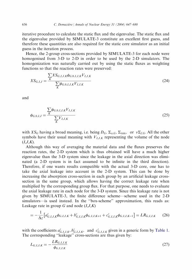
Hence, the 2-group cross-sections provided by SIMULATE-3 for each node werehomogenised from 3-D to 2-D in order to be used by the 2-D simulators. Thehomogenization was naturally carried out by using the static fluxes as weightingfunctions so that the reaction rates were preserved:

XSG;I;J ¼

PK

XSG;I;J;K�G;0;I;J;KVI;J;KPK

�G;0;I;J;KVI;J;Kð24Þ

and

�G;0;I;J ¼

PK

�G;0;I;J;KVI;J;KPK

VI;J;Kð25Þ

with XSG having a broad meaning, i.e. being DG;�a;G;�rem; or ��f;G: All the othersymbols have their usual meaning with VI;J;K representing the volume of the node(I,J,K).

Although this way of averaging the material data and the fluxes preserves thereaction rates, the 2-D system which is thus obtained will have a much highereigenvalue than the 3-D system since the leakage in the axial direction was elimi-nated (a 2-D system is in fact assumed to be infinite in the third direction).Therefore, if one wants results compatible with the actual 3-D core, one has totake the axial leakage into account in the 2-D system. This can be done byincreasing the absorption cross-section in each group by an artificial leakage cross-section in the same group, which allows having the correct leakage rate whenmultiplied by the corresponding group flux. For that purpose, one needs to evaluatethe axial leakage rate in each node for the 3-D system. Since this leakage rate is notgiven by SIMULATE-3, the finite difference scheme—scheme used in the 2-Dsimulators—is used instead. In the ‘‘box-scheme’’ approximation, this reads as:Leakage rate in group G and node (I,J,K)

¼ 1

DzazG;I;J;K�G;I;J;K þ bzG;I;J;K�G;I;J;Kþ1 þ czG;I;J;K�G;I;J;K1

� �¼ LRG;I;J;K ð26Þ

with the coefficients azG;I;J;K; bzG;I;J;K; and czG;I;J;K given in a generic form by Table 1.

The corresponding ‘‘leakage’’ cross-sections are thus given by:

LG;I;J;K ¼ LRG;I;J;K

�G;I;J;Kð27Þ


at the absorption cross-sections are modified in the following way:
so th
��a;G;I;J;K ¼ �a;G;I;J;K þ LG;I;J;K ð28Þ

The homogenization can then be carried out as described before, i.e. according to Eq.(24).

5. Static simulator

In this section, the algorithm used in the calculation of the static neutron flux andthe corresponding eigenvalue is highlighted. Since the estimation of the neutron fluxand the corresponding adjoint function have both some practical applications, andsince these two tasks are completely equivalent, both a forward static core simulatorand an adjoint static core simulator were actually developed and are reported in thefollowing.

Although the discretisation scheme was presented in Section 3 for the estimationof the neutron noise, it can be extended without any difficulty to the calculation ofthe static flux. For the sake of brevity, this derivation is not reported in this paper.One can easily show that the coupling coefficients are identical to the ones given inTable 1. The discretisation scheme thus allows writing the discretised form of the lefthand side of Eq. (5) for a node (I,J) in the following way:

r �D rð Þr þ�sta rð Þh i

�1;0 rð Þ

�2;0 rð Þ

� �� discrI;J

¼

��f;1;0;I;J

keff�a;1;0;I;J�rem;0;I;J

ax1;I;JDx

ay1;I;J

Dy��f;2;0;I;J

keff

�rem;0;I;J �a;2;0;I;J ax2;I;JDx

ay2;I;J

Dy

26664

37775

�1;0;I;J

�2;0;I;J

� �þ

bx1;I;JDx

0

0 bx2;I;JDx

2664

3775 �1;0;Iþ1;J

�2;0;Iþ1;J

� �þ

by1;I;J

Dy0

0 by2;I;J

Dy

26664

37775 �1;0;I;Jþ1

�2;0;I;Jþ1

� �

cx1;I;JDx

0

0 cx2;I;JDx

2664

3775

�1;0;I1;J

�2;0;I1;J

� �þ

cy1;I;J

Dy0

0 cy2;I;J

Dy

26664

37775

��1;0;I;J1

��2;0;I;J1

� �

ð29Þ


Forward calculations
5.1.
Regarding the calculation of the forward flux and the associated eigenvalue, Eq.(5) can be rewritten in a more convenient way:

�a;1;0;I;J þ�rem;0;I;J þax1;I;JDx

þay1;I;J

Dy0

�rem;0;I;J �a;2;0;I;J þax2;I;JDx

þay2;I;J

Dy

26664

37775

�1;0;I;J

�2;0;I;J

� �

þ

bx1;I;JDx

0

0bx2;I;JDx

2664

3775

�1;0;Iþ1;J

�2;0;Iþ1;J

� �þ

by1;I;J

Dy0

0by2;I;J

Dy

26664

37775

�1;0;I;Jþ1

�2;0;I;Jþ1

� �

þ

cx1;I;JDx

0

0cx2;I;JDx

2664

3775

�1;0;I1;J

�2;0;I1;J

� �þ

cy1;I;J

Dy0

0cy2;I;J

Dy

26664

37775

�1;0;I;J1

�2;0;I;J1

� �

¼1

keff

��f;1;0;I;J ��f;2;0;I;J

0 0

� �

�1;0;I;J

�2;0;I;J

� �ð30Þ

a generic form as follows:
or in
M � ¼1

keffF � ð31Þ

where � is a 2N vector column (N elements for the fast flux, and N elements for thethermal flux) if N is the total number of nodes of the system. The matrixes M and Fare 2N2N matrixes, but are obviously sparse.

The flux and the eigenvalue can then be searched for by using an iterative scheme.In the present study, the power iteration method was chosen for its simplicity and itsrelative efficiency (Bell and Glasstone, 1970; Nakamura, 1977). In such a method,the flux and the eigenvalue are given by the following expressions:

� nð Þ ¼ M1 1

kn1ð Þ

eff

F � n1ð Þ ð32Þ

and

knð Þ

eff ¼F � nð Þ

F � n1ð Þ k

n1ð Þ

eff ð33Þ

where (n) represents the iteration number. The starting point of this method is aninitial guess for � 0ð Þ and k

0ð Þ

eff . As mentioned previously, the values given by SIMU-LATE-3 were chosen. For the flux, the axially-condensed flux calculated accordingto Eq. (25) from the SIMULATE-3 results is actually used. Then, a new flux


distribution is calculated via Eq. (32), and subsequently a new eigenvalue is esti-mated via Eq. (33). This procedure is repeated until some convergence criteriaregarding both the neutron flux and the eigenvalue are fulfilled. Then the resultshave to be scaled since Eq. (31) is a homogeneous equation. The scaling factor iscalculated so that the power level corresponds to the one given by SIMULATE-3 inthe axially-condensed reactor:
X
fuel

�1;I;J�1;0;I;J þ �2;I;J�2;0;I;J

� ��static core simulator

¼Xfuel

�1;I;J�1;0;I;J þ �2;I;J�2;0;I;J

� ��SIMULATE3

ð34Þ

where �1,I,J and �2,I,J are the energy release per fast and thermal fission respectivelyfor a given node (I,J).

In the following, a benchmark between the static core simulator and SIMULATE-3 for a typical PWR is presented. This core actually corresponds to the SwedishRinghals-4 PWR (fuel cycle 16, cycle average burnup of 8.767 GWd/tHM). In sucha benchmark, the cross-sections used in the 2-D simulator were obviously obtaineddirectly from the 3-D core modelled in SIMULATE-3 without any modification ofthe absorption cross-sections (which would have been necessary to make in order totake the leakage in the axial direction into account, as described previously). Such across-section adjustment would have made the axially-condensed systems slightlydifferent with respect to the flux calculation. It is therefore expected that the eigen-value given by the static core simulator (2-D system) will be larger than the onegiven by SIMULATE-3 (3-D system) since the leakage in the axial direction is nottaken into account.

The results of the benchmarking are given in Figs. 2 and 3. The peaks observed inFig. 3 correspond to the reflector peaks, i.e. an increase of the thermal flux in thereflector region, and are also observed in the SIMULATE-3 results. As a result ofthe spatial discretisation, these peaks are higher when a reflector node is next to twofuel nodes. Furthermore, the agreement between the static core simulator andSIMULATE-3 is very good in the fuel zone. A more detailed analysis of the differ-ence between the 2-D static calculations and the SIMULATE-3 results would showthat the discrepancy is nevertheless relatively significant in the reflector zone forthree main reasons. First of all, the discretisation scheme used in the static coresimulator, i.e. the finite difference scheme, is known to give relatively poor resultswhen there are large flux gradients, such as for instance in the reflector region andclose to this region. SIMULATE-3 uses a nodal diffusion model, which gives muchmore accurate results in such cases. Another difference between the two modelling isthe number of nodes used in the calculation. In SIMULATE-3, the core is describedvia a 3232 lattice, whereas the static core simulator uses a 6464 lattice. In orderto compare the results of the two calculations, the SIMULATE-3 results weresimply expanded on the 6464 grid without any interpolation, i.e. the results arespatially homogeneous on each 22 node. Consequently, a reflector ‘‘assembly’’ isactually described by 22 nodes in the static core simulator, whereas it is described


Fig. 2. Static flux calculations in the fast group (the solution calculated by the 2-D 2-group static core simu-

lator is given in the upper figure, and the reference solution given by SIMULATE-3 is given in the lower figure).


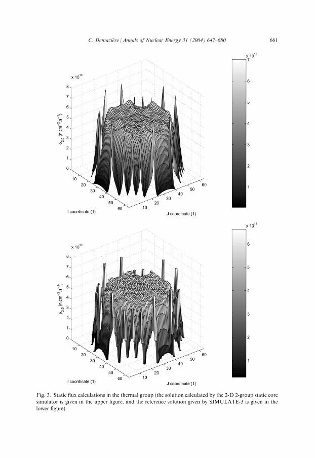
Fig. 3. Static flux calculations in the thermal group (the solution calculated by the 2-D 2-group static core

simulator is given in the upper figure, and the reference solution given by SIMULATE-3 is given in the

lower figure).


by only 11 node in SIMULATE-3. Since the static flux is assumed to vanish at thecore boundary, big discrepancies are thus expected in the reflector region. Finally,and most importantly, the edit of the cross-sections and fluxes by SIMULATE-3 isgiven for only one layer of reflector nodes surrounding the fuel region. It is veryunlikely that only one layer of nodes is used in the SIMULATE-3 calculations, oralternatively that the size of these reflector nodes are identical to the ones in the fuelregion. In the 2-D core simulator, all the nodes are assumed to have the samesize, and the layout of the core is derived from the SIMULATE-3 edit of thecross-sections. Thus, the modelling of the flux in the reflector nodes might bedifferent. Concerning the eigenvalue calculation, the static core simulator gives avalue of 1.00332, whereas SIMULATE-3 gives a value of 0.99998. This dis-crepancy was expected since the static core simulator represents a 2-D system inwhich the axial leakage was eliminated, whereas SIMULATE-3 represents an actual3-D system.

5.2. Adjoint calculations

For the sake of completeness, an adjoint static core simulator was also developed,since the calculation of the static adjoint function and eigenvalue is in many aspectsequivalent to the calculation of the forward static flux and its associated eigenvalue.There are several ways of defining an adjoint function, but it is common practice todefine it via the inner product of two flux functions ð Þ and � ð Þ, where representsthe variables of the phase space in which the functions are given. The inner productis then expressed as (Bell and Glasstone, 1970):

; �ð Þ ¼

ð� ð Þ �$ ð Þd ð35Þ

The adjoint L+ of the operator L is then defined as the one which satisfies

þ;L��

¼ Lþ þ; ��

ð36Þ

where + and �, which are the adjoint and forward functions respectively, satisfycertain boundary and continuity conditions. In 2-group diffusion theory, the adjointoperator is the transposed of the direct operator, so that the adjoint function can beeasily derived from Eq. (5) as:

r �D rð Þr þ�Tsta rð Þ

h i

�þ1;0 rð Þ�þ2;0 rð Þ

� �¼ 0 ð37Þ

We can then follow the same derivation as for the forward static core simulatorpresented in Section 5.1 to arrive to:


�a;1;0;I;J þ�rem;0;I;J þax1;I;JDx

þay1;I;J

Dy�rem;0;I;J

0 �a;2;0;I;J þax2;I;JDx

þay2;I;J

Dy

26664

37775

�þ1;0;I;J�þ2;0;I;J

" #

þ

bx1;I;JDx

0

0bx2;I;JDx

2664

3775

�þ1;0;Iþ1;J

�þ2;0;Iþ1;J

" #þ

by1;I;J

Dy0

0by2;I;J

Dy

26664

37775

�þ1;0;I;Jþ1

�þ2;0;I;Jþ1

" #

þ

cx1;I;JDx

0

0cx2;I;JDx

2664

3775

�þ1;0;I1;J

�þ2;0;I1;J

" #þ

cy1;I;J

Dy0

0cy2;I;J

Dy

26664

37775

�þ1;0;I;J1

�þ2;0;I;J1

" #

¼1

kþeff

��f;1;0;I;J 0

��f;2;0;I;J 0

� �

�þ1;0;I;J�þ2;0;I;J

" #

ð38Þ

or in a generic form

Mþ �þ ¼1

kþeffFþ �þ ð39Þ

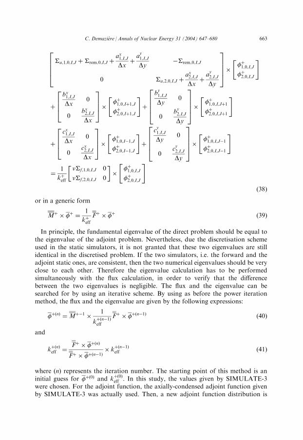
In principle, the fundamental eigenvalue of the direct problem should be equal tothe eigenvalue of the adjoint problem. Nevertheless, due the discretisation schemeused in the static simulators, it is not granted that these two eigenvalues are stillidentical in the discretised problem. If the two simulators, i.e. the forward and theadjoint static ones, are consistent, then the two numerical eigenvalues should be veryclose to each other. Therefore the eigenvalue calculation has to be performedsimultaneously with the flux calculation, in order to verify that the differencebetween the two eigenvalues is negligible. The flux and the eigenvalue can besearched for by using an iterative scheme. By using as before the power iterationmethod, the flux and the eigenvalue are given by the following expressions:

�þ nð Þ ¼ Mþ1 1

kþ n1ð Þ

eff

Fþ �þ n1ð Þ ð40Þ

and

kþ nð Þ

eff ¼Fþ �þ nð Þ

Fþ �þ n1ð Þ k

þ n1ð Þ

eff ð41Þ

where (n) represents the iteration number. The starting point of this method is aninitial guess for �þ 0ð Þ and k

þ 0ð Þ

eff . In this study, the values given by SIMULATE-3were chosen. For the adjoint function, the axially-condensed adjoint function givenby SIMULATE-3 was actually used. Then, a new adjoint function distribution is


calculated via Eq. (40), and subsequently a new eigenvalue is estimated via Eq. (41).This procedure is repeated until some convergence criteria regarding both theadjoint function and the eigenvalue are fulfilled. Then the results have to be scaledsince Eq. (39) is a homogeneous equation. The scaling is required for comparisonpurposes between the adjoint core simulator and SIMULATE-3. The scaling factoris calculated so that the volume integral of the fast adjoint function is equal to unity:

1

Nfuel�fuel�þ1;0;I;J ¼ 1 ð42Þ

where Nfuel is the number of nodes in the fuel region.This adjoint core simulator was then benchmarked against SIMULATE-3, by

using the same set of data as for the benchmark of the forward static core simulator.In such a benchmark, the cross-sections used in the 2-D simulator were once againobtained directly from the 3-D core modelled in SIMULATE-3 without any modifi-cation of the absorption cross-sections. It is therefore expected that the eigenvalue givenby the adjoint core simulator (2-D system) will be larger than the one given by SIMU-LATE-3 (3-D system) since the leakage in the axial direction is not taken into account.

The results of the benchmarking are given in Figs. 4 and 5. As can be seen in thesefigures, the agreement between the adjoint core simulator and SIMULATE-3 is verygood in the fuel zone. A more detailed analysis of the difference between the 2-Dstatic calculations and the SIMULATE-3 results would show that the discrepancy isrelatively significant in the reflector zone. The same reasons as the ones presented forthe static core simulator could explain this discrepancy, i.e. the difference in thespatial discretisation schemes between SIMULATE-3 and the adjoint core simu-lator, the different number of nodes used for the calculations, and the possibledifference of the modelling of the reflector region between the adjoint staticcore simulator and SIMULATE-3. Concerning the eigenvalue calculation, theadjoint core simulator gives a value of 1.00332, whereas SIMULATE-3 gives a valueof 0.99998 for kþeff . These values are identical to the ones given by the forwardstatic calculations, as expected. The discrepancy between the SIMULATE-3 andthe adjoint core simulator results was expected since the adjoint core simulatorrepresents a 2-D system in which the axial leakage was eliminated, whereasSIMULATE-3 represents an actual 3-D system.

6. Dynamic simulator

In this section, the algorithm used in the calculation of the neutron noise is high-lighted. As for the static calculations, the estimation of the neutron noise and thecorresponding adjoint function have both some practical applications. Since thesetwo tasks are completely equivalent, both a forward and an adjoint dynamic coresimulators were actually developed and are reported in the following.

Before turning to the algorithms used for the calculation of the neutron noise, it isadvisable to point out what kind of noise sources the neutron noise simulator canmodel. It is well known in power reactor noise analysis that localised noise sources


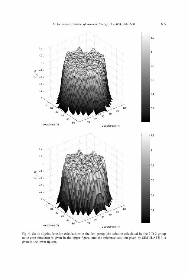
Fig. 4. Static adjoint function calculations in the fast group (the solution calculated by the 2-D 2-group

static core simulator is given in the upper figure, and the reference solution given by SIMULATE-3 is

given in the lower figure).


Fig. 5. Static adjoint function calculations in the thermal group (the solution calculated by the 2-D

2-group static core simulator is given in the upper figure, and the reference solution given by SIMULATE-3

is given in the lower figure).


can be classified into two categories, usually referred to as a vibrating absorber, andan absorber of variable strength or reactor oscillator (Bell and Glasstone, 1970). Thefirst one is typically represented by the lateral vibrations of a control rod in a PWR.The second one is due to time-varying cross-sections at a fixed point. Whereas themathematical treatment of the neutron noise induced by a vibrating absorber ismuch more complicated than of the neutron noise induced by an absorber ofvariable strength, only the vibrating absorber case was given any significantattention so far. As can be seen in the derivation of Eq. (8), the neutron noisesimulator is able to model noise sources of the ‘‘absorber of variable strengthtype’’. Nevertheless, the noise source induced by a ‘‘vibrating absorber type’’ ofnoise source can be estimated from the gradient of the neutron noise induced byan ‘‘absorber of variable strength’’ type of noise source located at the equilibriumposition of the vibrating rod as explained in the following. A vibrating absorbercan be modelled as being a 1-D structure that vibrates perpendicular to a 2-Dplane and that always remains parallel to itself. Consequently, the problem can becorrectly treated in this 2-D plane by assuming that the noise source is describedby (Williams, 1974):

�XS r; tð Þ ¼ � � � r rp " tð Þ� �

� r rp� ��

ð43Þ

where � is the strength of the perturbation, and rp its equilibrium position in the Fein-berg–Galanin model. The vector " tð Þ describes the 2-D vibrations of the noise sourcearound its equilibrium position. If one calculates now the neutron noise induced by apoint-source located at rp that has the same nature as the noise source modelled byEq. (43), i.e. a perturbation of the fast and/or thermal absorption cross-section, aperturbation of the fast and/or thermal fission cross-section, a perturbation of theremoval cross-section, the neutron noise simulator actually estimates the so-called2-group Green’s function defined from Eq. (8) as follows:


h i G�XS r; rp; !

� �¼ �XS r rp

� �ð44Þ

For the sake of brevity, the noise source in Eq. (44) is simply written as�XS r rp

� �, which is a two-component vector. Depending on the nature of the noise

source in Eq. (43), the exact expression of the noise source �XS r rp� �

can be derivedfrom the right hand side of Eq. (8). For example, the noise source in case offluctuations of the macroscopic removal cross-section is given as:

�rem r rp� �

¼�1;0 rð Þ� r rp

� ��1;0 rð Þ� r rp

� �� ð45Þ

The Green’s function fulfilling Eq. (44) is slightly different from its usual definition[see for instance (Pazsit and Glockler, 1983)].

Using a one-term Taylor expansion in " tð Þ, the neutron noise induced by thevibrating noise source defined in Eq. (43) can then be calculated as (Pazsit andGlockler, 1983):


��1 r; !ð Þ

��2 r; !ð Þ

� �¼ � � " !ð Þ � rrp G�XS r; rp; !

� �� ð46Þ

Consequently, the neutron noise induced by a vibrating noise source can be cal-culated by using the neutron noise simulator to first estimate the Green’s function,and then applying Eq. (46). The application of Eq. (46) is actually rather difficultsince it requires the calculation of the derivative of the Green’s function withrespect to the second variable, i.e. the equilibrium position of the noise source. Aswill be seen in Section 6.2, the estimation of the adjoint Green’s function instead ofthe forward Green’s function allows circumventing this problem. This means thatthe neutron noise simulator is able to estimate the spatial distribution of theneutron noise induced either by an ‘‘absorber of variable strength’’ type of noisesource or a ‘‘vibrating absorber’’ type of noise source in the 2-group diffusionapproximation.

Coming back to the neutron noise simulator itself and to the way Eq. (8) issolved, the discretisation scheme presented in Section 3 allows writing thediscretised form of the left hand side of Eq. (8) for a node (I,J) in the followingway:


h i

��1;0 r; !ð Þ

��2;0 r; !ð Þ

� �� discrI;J

¼

�1;I;J !ð Þax1;I;JDx

ay1;I;J

Dy��f:2;0;I;J

keff1

i!�effi!þ l

�rem;0;I;J �a;2;0;I;Jþi!

v2

ax2;I;JDx

ay2;I;J

Dy

26664

37775 ��1;I;J !ð Þ

��2;I;J !ð Þ

� �

þ

bx1;I;JDx

0

0 bx2;I;JDx

2664

3775 ��1;Iþ1;J !ð Þ

��2;Iþ1;J !ð Þ

� �þ

by1;I;J

Dy0

0 by2;I;J

Dy

26664

37775 ��1;I;Jþ1 !ð Þ

��2;I;Jþ1 !ð Þ

� �

þ

cx1;I;JDx

0

0 cx2;I;JDx

2664

3775 ��1;I1;J !ð Þ

��2;I1;J !ð Þ

� �þ

cy1;I;J

Dy0

0 cy2;I;J

Dy

26664

37775 ��1;I;J1 �!ð Þ

��2;I;J1 !ð Þ

� �

ð47Þ

6.1. Forward calculations

Regarding the calculation of the neutron noise, Eq. (8) can be rewritten in a moreconvenient way:


�1;I;J !ð Þ ax1;I;JDx

ay1;I;J

Dy��f;2;0;I;J

keff1

i!�effi!þ l

�rem;0;I;J �a;2;0;I;J þi!

v2

ax2;I;JDx

ay2;I;J

Dy

26664

37775

��1;I;J !ð Þ

��2;I;J !ð Þ

� �

þ

bx1;I;JDx

0

0 bx2;I;JDx

2664

3775

��1;Iþ1;J !ð Þ

��2;Iþ1;J !ð Þ

� �þ

by1;I;J

Dy0

0 by2;I;J

Dy

26664

37775

��1;I;Jþ1 !ð Þ

��2;I;Jþ1 !ð Þ

� �

þ

cx1;I;JDx

0

0 cx2;I;JDx

2664

3775

��1;I1;J !ð Þ

��2;I1;J !ð Þ

� �þ

cy1;I;J

Dy0

0 cy2;I;J

Dy

26664

37775

��1;I;J1 !ð Þ

��2;I;J1 !ð Þ

� �

¼�1;0;I;J

�1;0;I;J

� � ��rem;I;J !ð Þ þ

�1;0;I;J 0

0 �2;0;I;J

� �

��a;1;I;J !ð Þ

��a;2;I;J !ð Þ

� �

þ�1;0;I;J

keff1

i!�effi!þ l

�2;0;I;J

keff1

i!�effi!þ l

0 0

24

35

��f;1;I;J !ð Þ

��f;2;I;J !ð Þ

� �

ð48Þ

or in a generic form as follows:

N !ð Þ �� !ð Þ ¼ �S !ð Þ ð49Þ

Eq. (49) represents an heterogeneous equation, which can be directly inverted inorder to provide the flux noise as:

�� !ð Þ ¼ N1 !ð Þ �S !ð Þ ð50Þ

Consequently, the estimation of the neutron noise is in some aspects simpler thanthe estimation of the static flux, which is described by an eigenvalue equation. Onthe other hand, the neutron noise simulator relies on complex arithmetic, whichrenders the calculations more difficult than for the static cases.

As for the static core simulators, a benchmark of the dynamic core simulator wascarried out. Nevertheless, since no other dynamic core simulator was available at theDepartment of Reactor Physics, Chalmers University of Technology, the bench-marking of the numerical solution was performed against analytical solutions. Forthe sake of simplicity, it is assumed in the following that the noise source for thebenchmark cases is a point-source located at the core centre, and that the core isspatially homogeneous. This allows having a relatively simple expression for theanalytical solution. The material constants and the point-kinetic parameters corres-pond to a generic General Electric BWR/6, whereas the core layout is representative


of the Swedish Forsmark-1 BWR. Three different cases were considered: a noisesource defined in terms of the fluctuation of the fast absorption cross-section, one ofthe thermal absorption cross-section, and finally one of the removal cross-section.The accuracy of the neutron noise simulator was found to be completely indepen-dent of the type of noise source investigated. Therefore, in the following, only thecase of a macroscopic removal cross-section noise is presented. Since the noisesource was located in the middle of the core, the results are rotational-invariantaround the z-axis crossing the core centre. Therefore only the radial dependence ofthe fluxes is accounted for in the following. As pointed out previously, a static cal-culation using the static core simulator is also required before using the neutronnoise simulator, so that the reactor is critical when applying the discretisationscheme based on finite differences. Likewise, the eigenvalue has to be determinedprior to the calculation of the analytical solution. For that purpose, the reactorbuckling was estimated assuming that both the fast and thermal static fluxes weredistributed according to the fundamental mode. The analytical calculation of theneutron noise can then be performed by solving the following equation:


h i

��1 r; !ð Þ

��2 r; !ð Þ

� �¼ G �rem rð Þ� rð Þ ð51Þ

where G is the noise source strength. This coefficient allows also taking into accountthe fact that the noise source is homogeneously distributed over one or several nodesin the numerical solution (the nodes representing the core centre), and therefore isnot a point-source. Consequently, the G coefficient is adjusted so that the noisesource has the same strength in the analytical solution as in the numerical one. Theanalytical solution is thus simply given by:

��1 r; !ð Þ ¼ A K0 lrð Þ þ B I0 lrð Þ þ C Y0 �rð Þ þD J0 �rð Þ ð52Þ

��2 r; !ð Þ

¼ A cl K0 lrð Þ þ B cl I0 lrð Þ þ C c� Y0 �rð Þ þD c� J0 �rð Þ

ð53Þ

where l2 and �2 are the two eigenvalues of the following matrix:

�1 !ð Þ

D1

��f;2;0

keffD11

i!�effi!þ l

�rem;0

D2

1

D2�a;2;0 þ

i!

v2

2664

3775 ð54Þ

and the coupling coefficient cl and c� are given as follows:

cl ¼�rem;0

�a;2;0 þi!

v2

D2l

2

ð55Þ


c� ¼�rem;0

�a;2;0 þi!

v2

þD2�2

ð56Þ

The coefficients A, B, C, and D are solutions of the following equation, whichexpresses the fact that the neutron noise vanishes at the boundary of the system andthat the current noise is driven by the central noise source:

K0 lRð Þ I0 lRð Þ Y0 �Rð Þ J0 �Rð Þ

cl K0 lRð Þ cl I0 lRð Þ c� Y0 �Rð Þ c� J0 �Rð Þ

1 0 �r Y1 �Rð Þ½ �r ! 0 0

cl 0 c� �r Y1 �rð Þ½ �r ! 0 0

26664

37775

A

B

C

D

26664

37775

¼

0

01

2�D1G �1;0 0ð Þ

1

2�D2G �1;0 0ð Þ

26666664

37777775

ð57Þ

In the previous equations, R is the core radius and the function In, Jn, Kn, and Yn arethe modified Bessel function of the first kind, the Bessel function of the first kind, themodified Bessel function of the second kind, and the Bessel function of the secondkind, respectively with n being the order of the different functions.

Figs. 6 and 7 depict the amplitude of the flux noise and its phase for both theanalytical solution and the numerical one at a frequency of 0.5 Hz. Since the noisesimulator calculates a spatially-averaged flux noise over each node, the analyticalsolution was also averaged on each node, so that both solutions could be directlycompared. Furthermore, due to the difference in the modelling of the noise source inthe numerical and analytical solutions, i.e. its finite spatial distribution and its point-like character respectively, the flux noise differs between the two solutions. Althoughthe G coefficient allows scaling the analytical solution to the numerical one, the twosolutions are different in the nodes where the noise source is located for the numer-ical problem. Consequently, the numerical and analytical solutions are only given inFigs. 6 and 7 for positions further away from the noise source. It can be noticed thatthe agreement between the analytical and the numerical solutions is excellent, forboth the magnitude and the phase of the flux noise, both in the fast and thermalgroups.

6.2. Adjoint calculations

As will be seen in the following, the calculation of the adjoint function is asinteresting as the calculation of the neutron noise and has many practical applica-tions. In this Section, the development and benchmarking of an adjoint dynamic


Fig. 6. Comparison between the numerical and the analytical fast flux noise at a frequency of 0.5 Hz.


Fig. 7. Comparison between the numerical and the analytical thermal flux noise at a frequency of 0.5 Hz.


core simulator is reported. The same conventions and definitions of the adjointfunctions and operators as the ones presented in Section 5.2 are used in this section. In2-group diffusion theory, the adjoint operator is simply the transposed of the directoperator, so that the adjoint function can be easily derived from Eq. (8). It is actuallyadvantageous to calculate the adjoint function for a point-like source located at aposition r0. In such a case the adjoint function is solution of the following Equation:

r �D rð Þr þ�Tdyn r; !ð Þ

h i

��þ1 r; !ð Þ

��þ2 r; !ð Þ

� �¼

� r r0ð Þ

� r r0ð Þ

� �ð58Þ

For the sake of completeness, the source term in Eq. (58) is defined in both the fastand the thermal group. In some cases, such as calculating the response of a detectorto a noise source, it is more convenient to define the source term for the adjointproblem in the thermal group only, since detectors are very often sensitive to thethermal flux only. From Eq. (58), we can then follow the same derivation as for theforward dynamic core simulator presented in Section 6.1 to arrive at:

�1;I;J !ð Þ ax1;I;JDx

ay1;I;J

Dy�rem;0;I;J

��f;2;0;I;J

keff1

i!�effi!þ l

�a;2;0;I;J þ

i!

v2

ax2;I;JDx

ay2;I;J

Dy

26664

37775

��þ1;I;J !ð Þ

��þ2;I;J !ð Þ

" #

þ

bx1;I;JDx

0

0 bx2;I;JDx

2664

3775

��þ1;Iþ1;J !ð Þ

��þ2;Iþ1;J !ð Þ

" #þ

by1;I;J

Dy0

0 by2;I;J

Dy

26664

37775

��þ1;I;Jþ1 !ð Þ

��þ2;I;Jþ1 !ð Þ

" #

þ

cx1;I;JDx

0

0 cx2;I;JDx

2664

3775

��þ1;I1;J !ð Þ

��þ2;I1;J !ð Þ

" #þ

cy1;I;J

Dy0

0 cy2;I;J

Dy

26664

37775

��þ1;I;J1 !ð Þ

��þ2;I;J1 !ð Þ

" #

¼� I I0; J J0ð Þ

� I I0; J J0ð Þ

� �ð59Þ

or in a generic form:

Nþ !ð Þ ��þ !ð Þ ¼ �Sþ !ð Þ ð60Þ

Eq. (60) represents an heterogeneous equation, which can be directly inverted inorder to provide the adjoint function as:

��þ !ð Þ ¼ Nþ1 !ð Þ �Sþ !ð Þ ð61Þ

As for the forward dynamic core simulator, it is possible to benchmark the adjointdynamic core simulator against analytical solutions in some simplified cases.


Nevertheless, since the forward dynamic core simulator was already successfullybenchmarked against analytical solutions, the adjoint dynamic core simulator canbe benchmarked against the direct calculations by using the properties of the adjointoperators. This task is actually more challenging than the benchmarking againstanalytical solutions, since it can be done with strongly heterogeneous cores. In thefollowing, a BWR representative of the Swedish Forsmark-1 core (fuel cycle 16,middle of cycle conditions) was chosen. The starting point is to use Eq. (36), whichcan be rewritten as follows:

��þ;L��

¼ Lþ��þ; ��

ð62Þ

+
where the operators L and L can be formally defined from Eqs. (8) and (58),respectively, as:
L�� ¼ �S ð63Þ

and

Lþ��þ ¼ �Sþ: ð64Þ

If the noise source in the forward problem is, as in the adjoint problem, a point-like source, this time located at rS, i.e.

�S r; !ð Þ ¼�1� r rSð Þ

�2� r rSð Þ

� �; ð65Þ

Eq. (62) gives:
ð��þ1 r; r0; !ð Þ
��þ2 r; r0; !ð Þ

� ��1� r rSð Þ

�2� r rSð Þ

� �dr ¼

ð� r r0ð Þ

� r r0ð Þ

� ��1 r; rS; !ð Þ

��2 r; rS; !ð Þ

� �dr ð66Þ

and thus:

�1��þ1 rS; r0; !ð Þ þ �2��

þ2 rS; r0; !ð Þ ¼ ��1 r0; rS; !ð Þ þ ��2 r0; rS; !ð Þ ð67Þ

It can be seen from Eq. (67) that the adjoint function actually allows estimatingthe neutron noise at the position r0 induced by a noise source located in rS. If r0

coincides with the location of a neutron detector, the adjoint function is propor-tional to the sensitivity of the detector to fluctuations. This sensitivity is sometimescalled the field-of-view of the detector (van Dam, 1975). Furthermore, the left handside of Eq. (67) is given by the adjoint solution, whereas the right hand side of Eq. (67)is given by the forward solution. This opens up the possibility of benchmarking theadjoint dynamic core simulator. Such a benchmarking is presented in Figs. 8 and 9 ata frequency of 1 Hz, where the noise source in the forward problem was chosen tobe defined via the fluctuations of the macroscopic removal cross-section, i.e.

�S r; !ð Þ ¼� r rSð Þ�1;0 rð Þ� r rSð Þ�1;0 rð Þ

� �ð68Þ

which is equivalent to saying that �1=�1,0(rS) and �2=�1,0(rS). As can be seen inFigs. 8 and 9, the agreement between the adjoint and forward solutions is excellent.


Fig. 8. Comparison between the amplitude of the neutron noise given by the adjoint calculation (upper

figure) and the forward calculation (lower figure) at a frequency of 1 Hz.


Fig. 9. Comparison between the phase of the neutron noise given by the adjoint calculation (upper figure)

and the forward calculation (lower figure) at a frequency of 1 Hz.


As pointed out by Pazsit (1992), the calculation of the adjoint dynamic transferfunction is advantageous in cases when one wants to determine the neutron noise ata given position in the core, for instance where a neutron detector is located, forseveral positions of the noise source. For cases where the neutron noise is searchedfor at many positions in the core for one given noise source, the forward approach ismore practical. Another advantage of the adjoint dynamic core simulator is thepossibility of modelling the ‘‘vibrating absorber’’ type of noise source. As pointedout previously, the so-called discretised forward Green’s function, which is actuallycalculated by the forward dynamic core simulator, allows estimating the neutronnoise for this kind of noise source, as was demonstrated in Eq. (46). Nevertheless,applying Eq. (46) is rather difficult since it requires the calculation of the derivativeof the Green’s function with respect to the second variable, i.e. the equilibriumposition of the noise source. By using the adjoint approach instead, it can easily beshown that the neutron noise can be inferred from the following equation:

��1 r0; !ð Þ

��2 r0; !ð Þ

� �¼ � � " !ð Þ � rrp Gþ

�XS rp; r0; !� ��

ð69Þ

Compared to Eq. (46), calculating the derivative of the adjoint Green’s functionwith respect to the first variable is rather easy, since the full space dependence of theadjoint Green’s function with respect to the first variable is known. As before, theadjoint approach allows determining the induced flux noise at the position r0, andtherefore is only advantageous if one wants to estimate the response of one singleneutron detector. If the determination of the neutron noise in several locations isrequired, only the forward approach is applicable, but it supposes the prior knowl-edge of the derivative of the forward Green’s function with respect to the secondvariable.

7. Conclusions

In this paper, numerical tools for power reactor noise analysis were reported.More specifically, a dynamical core simulator and a static core simulator bothrelying on the 2-group diffusion approximation and finite differences weredeveloped for modelling 2-dimensional heterogeneous systems. The dynamicalsimulator allows estimating the neutron noise and the corresponding adjointfunction, whereas the static core simulator allows determining the static flux, thecorresponding adjoint function, and their associated eigenvalues. From a set ofdata—the point-kinetic parameters and 2-group material constants of the core—representative of the actual operating conditions of any type of reactor, thedynamical core simulator calculates the so-called reactor transfer function, i.e. thespatial distribution of the neutron noise induced by any type of spatially distributedor localised noise sources in the core. The prior use of the static core simulator isrequired to assure that the static equations are fulfilled with a discretisation schemecompatible with the dynamic calculations. Benchmarking of these simulatorsrevealed that they were working satisfactorily.


These numerical tools have already been applied to several practical cases, as thelocalisation of an unseated fuel assembly in the Swedish Forsmark-1 BWR channelinstability event (Demaziere and Pazsit, 2001), the explanation of the strong space-dependence of the Decay Ratio during the same event (Demaziere and Pazsit,2003a), and also the explanation of the underestimation of the MTC by noise ana-lysis in PWRs (Demaziere and Pazsit, 2003b). All these cases required the calcula-tion of the dynamical reactor transfer function of the corresponding reactors.Therefore, such applications would have been impossible without the developmentof the neutron noise simulator presented in this paper.

At this stage, the noise sources that the neutron noise simulator can handle haveto be defined directly from the fluctuations of the macroscopic cross-sections. Thedevelopment of a thermal-hydraulic module is planned in the future, so that a morestraightforward definition of the noise sources in the reactor would be possible. Forthat purpose, the simulators should also be able to model 3-dimensional systems.Another further development of the neutron noise simulator would be the type ofsystems that can be modelled. So far, only PWR and BWR cases, i.e. Light WaterReactor (LWR) cases, were investigated. Some work is currently under way tohandle CANDU reactors, and also subcritical source-driven systems. For theformer, the much longer diffusion length makes this kind of reactor particularlyinteresting, since the relaxation length of the local component of the neutron noise,related to local disturbances [as opposed to the global component related to thecoupled behaviour of the neutron noise over the whole core (Wach and Kosaly,1974), (Behringer et al., 1977)], will be much larger than for LWRs. For the latter,the equations have to be slightly modified due to the presence of an external neutronsource. Although the neutron noise simulator relies on linear theory, i.e. small fluc-tuations, the case of a source perturbation does not require such an approximation.A practical application of this would be the modelling of reactor transients due to abeam trip in ADS—Accelerator Source Driven—systems for instance.

Acknowledgements

The Swedish Nuclear Power Inspectorate (SKI - Statens Karnkraftinspektion) isacknowledged for its financial support during the development of the neutron noisesimulator. Professor Imre Pazsit is also deeply acknowledged for his commentsregarding both this work and this paper.

References

Analytis, G.Th., 1982. Frequency response of the neutron field to localized perturbations in a 3-D

heterogeneous lattice and applications. Annals of Nuclear Energy 9 (11–12), 601–613.

Antonopoulos-Domis, M., Skarpeta, K., 1986. Decomposition of neutron noise in a heterogeneous

reactor model into a local and a global component. Atomkernenergie Kerntechnik 48 (4), 221–223.

Behringer, K., Kosaly, G., Kostic, Lj., 1977. Theoretical investigation of the local and global components

of the neutron-noise field in a boiling water reactor. Nuclear Science and Engineering 63 (3), 306–318.


Bell, G.I., Glasstone, S., 1970. Nuclear Reactor Theory. Van Nostrand Reinhold Company, New York.

Covington, L.J., 1995. SIMULATE-3: Advanced Three-Dimensional Two-Group Reactor Analysis

Code—User’s Manual. Studsvik/SOA-95/15.

van Dam, H., 1975. A perturbation method for analysis of detector response to parametric fluctuations in

reactors. Atomkernenergie 25 (1), 70–71.

van Dam, H., 1976. Neutron noise in boiling water reactors. Atomkernenergie 27 (1), 8–14.

D’Auria, F. et al., 1997. State of the Art Report on Boiling Water Reactor Stability. NEA/CSNI/R(96)21.

Demaziere, C., Pazsit, I., 2001. 2-D 2-group neutron noise simulator and its application to anomaly

localisation. In: Proceedings of the International Meeting on Mathematical Methods for Nuclear

Applications (M&C2001), Salt Lake City, Utah, USA, 9–13 September, 2001, American Nuclear

Society.

Demaziere, C., Pazsit, I., 2003a. A phenomenological model for the explanation of a strongly space-

dependent decay ratio. In: Proceedings of the International Meeting on Nuclear Mathematical and

Computational Sciences (M&C2003), Gatlinburg, Tennessee, USA, 6–11 April, 2003, American

Nuclear Society.

Demaziere, C., Pazsit, I., 2003b. Development of a method for measuring the MTC by noise analysis and

its experimental verification in Ringhals-2. Nuclear Science and Engineering. (accepted).

Ekberg, K., Forssen, B.-H., Knott, D., 1995. CASMO-4: A Fuel Assembly Burnup Program—User’s

Manual. Studsvik/SOA-95/1.

van der Hagen, T.H.J.J., Hoogenboom, J.E., van Dam, H., 1992. A multidimensional multigroup model

for the determination of the frequency-dependent field of view of a neutron detector. Nuclear Science

and Engineering 110 (3), 237–253.

Khericha, S.T., 2001. Development of two-energy group, two-dimensional, frequency dependent detector

adjoint function based on the nodal method. Annals of Nuclear Energy 28 (11), 1049–1068.

Nakamura, S., 1977. Computational Methods in Engineering and Science with Applications to Fluid

Dynamics and Nuclear Systems. Wiley Interscience, New York.

Pazsit, I., 1992. Dynamic transfer function calculations for core diagnostics. Annals of Nuclear Energy 19

(5), 303–312.

Pazsit, I., Glockler, O., 1983. On the neutron noise diagnostics of pressurized water reactor control rod

vibrations. I. Periodic vibrations. Nuclear Science and Engineering 85 (2), 167–177.

Thie, J.A., 1963. Reactor Noise. Rowman and Littlefield, Inc, New York.

Thie, J.A., 1981. Power Reactor Noise. American Nuclear Society, La Grange Park, IL.

Uhrig, R.E., 1970. Random noise techniques in nuclear reactor systems. The Ronald Press Company,

New York.

Wach, D., Kosaly, G., 1974. Investigation of the joint effect of local and global driving sources in incore-

neutron noise measurements. Atomkernenergie 23 (4), 244–250.

Williams, M.M.R., 1967. Reactor noise in heterogeneous systems: I. Plate-type elements. Nuclear Science

and Engineering 30 (2), 188–198.

Williams, M.M.R., 1974. Random Processes in Nuclear Reactors. Pergamon Press, Oxford.


development of a 2-d 2-group neutron noise simulator

Documents