development and validation of a generic 3d model of the ...eprints.qut.edu.au/5636/1/5636.pdf ·...

COVER SHEET

This is the author-version of article published as: Schmutz, Beat and Reynolds, Karen J. and Slavotinek, John P. (2006) Development and validation of a generic 3D model of the distal femur. Computer Methods in Biomechanics and Biomedical Engineering 9(5):pp. 305-312. Accessed from http://eprints.qut.edu.au © 2006 Taylor & Francis

http://eprints.qut.edu.au/

Development and validation of a generic 3D model of the distal femur Dr. Beat Schmutz Institute of Health and Biomedical Innovation Queensland University of Technology 60 Musk Avenue Kelvin Grove Brisbane, QLD 4059 Australia Ph: +61 7 3138 6291 Fax: +61 7 3138 6030 E-mail: [email protected] A/Prof. Karen J. Reynolds School of Informatics & Engineering Flinders University GPO Box 2100 Adelaide SA 5001, Australia Tel: +61 8 8201 5190 Fax: +61 8 8201 3618 E-mail: [email protected] Dr. John P. Slavotinek Division of Medical Imaging Flinders Medical Centre Bedford Park SA 5042, Australia Tel: +61 8 8204 4154 Fax: +61 8 8374 1731 E-mail: [email protected]

1

mailto:[email protected]



Abstract

The development and validation of a virtual generic 3D model of the distal femur using

computer graphical methods is presented. The synthesis of the generic model requires

the following steps: acquisition of bony 3D morphology using standard CT (computed

tomography) imaging; alignment of 3D models reconstructed from CT images with a

common coordinate system; computer graphical sectioning of the models; extraction of

bone contours from the image sections; combining and averaging of extracted contours;

and 3D reconstruction of the averaged contours.

The generic models reconstructed from the averaged contours of six cadaver

femora were validated by comparing their surface geometry on a point to point basis

with that of the CT reconstructed reference models. The mean errors ranged from 0.99 -

2.5 mm and were in agreement with the qualitative assessment of the models.

Keywords

Generic 3D model; Femur; 3D contour reconstruction; 3D model alignment, Cadaveric

study

2

1 Introduction

Today a vast amount of literature exists on the anatomy and function of the knee joint

(for reviews see [1-3]). Despite this, controversy still exists regarding the exact shape of

the femoral condyles [4,5]. It is the geometry of the articulating surfaces of the knee

joint that contributes significantly to the movement pattern of the joint [5-7]. Therefore

the 3D morphology of the distal femur is of particular importance to the design of knee

replacement components. Although total knee replacement (TKR) surgery generally

enjoys a high success rate, with the increasing activity demand of patients there is a

need to improve the function and longevity of knee implants [8]. Given that knee

function and movement pattern of the femur are related to morphology, the capacity to

quantify morphology of the distal femur may assist design of joint replacement

components.

The 3D morphology of the distal femur has been quantified using various data

acquisition methods. Wismans et al. [9] developed a dial gauge to measure 50 – 100

points on each condyle of one cadaver specimen. Martelli et al. [10] used a FARO arm

electrogoniometer (accuracy 0.3 mm) to digitise the articulating surfaces of the distal

femur of six cadaver specimens. Ghosh [11] developed a close-range photogrammetric

3D mapping system (accuracy 0.2 mm) for the perspective diagramming of the knee

joint. Huiskes et al. [12] used an analytical stereophotogrammetric method (accuracy

0.2 mm) to measure the 3D articular geometry of a pair of knee joints. Siu et al. [13]

manually digitised the bone outlines from transverse CT scan images of five cadaver

specimens. In their study Siu and colleagues employed a calibration frame to

standardise positioning of the resected cadaver specimens during CT imaging.

3

All of the above studies were based on relatively small data sets of 1-6 cadaver

specimens. However, larger data sets are required in order to construct an average shape

of the condylar articulating surfaces representative of a larger population sample.

None of these data acquisition methods is particularly well suited for such a task

as they either require dissection of the joint and/or rely on specialist equipment that is

generally not present in hospitals. This study proposes a simpler data acquisition

method which makes use of CT images that have been acquired without a calibration

frame. The significant advantage of this approach is that it enables the development of a

generic model of the femur using existing (or newly acquired) CT scan image data from

a range of hospitals. Hence, a potentially greater and more age diverse source of image

data would be accessible.

The purpose of this study was to provide a quantitative answer to the question:

‘How well does a generic 3D model resemble a particular model of the distal femur?’

The method used to quantify the difference between two models was based on

calculating the disparity between the surface geometry of two models on a point to point

basis. To the best knowledge of the authors, such a comparison (on a point to point

basis) between a generic model and individual femur models has not yet been reported

in the literature.

2 Materials and Methods

2.1 Image data acquisition & 3D model reconstruction

4

CT scan data was obtained from the distal femur of nine intact embalmed human

cadaver lower limbs, made available by the Department of Anatomy & Histology of the

School of Medicine, Flinders University, South Australia. The average age of the

specimens was 80 years (range 72 - 89). Only right knees were available from five male

and four female donors.

Each leg was positioned in the centre of the scan field to minimise beam

hardening and partial volume effect [14]. This was achieved by aligning the longitudinal

axis of the leg with the scanning axis. The images were acquired in a helical mode with

a CT scanner (HiSpeed CT/i, General Electric Medical Systems) at the Flinders Medical

Centre, Adelaide, operating at 120 kV, 150 mA, with a pitch of 1.5:1 and a gantry

rotation time of 0.8 seconds. With all slices overlapping by 50% the effective slice

spacing was 0.5 mm for the condylar region and 1.5 mm for the diaphysis. From each

femur about 155 transverse image slices with a pixel size of 0.33 mm were obtained.

The image data were transferred to a PC (Pentium III, 1 GHz, 256 MB RAM) where 3D

models of the distal femora were reconstructed with an accuracy of 0.5 mm using

Mimics 7.30 software (Materialise, Leuven, Belgium) [15]. After their reconstruction

the 3D models were saved in DXF-file format such that they could be imported as

polygon mesh objects into IDL 5.5 (Research Systems Inc, Boulder, USA) for further

processing.

A visual inspection of the reconstructed models revealed that two of the models

were not suitable to be included in the data set used to develop a generic model of the

femur. One of the models displayed significant marginal osteophytes (a manifestation of

osteoarthrosis, a common degenerative condition), and the other exhibited a deep

‘groove’ on the anterior aspect of the condyles most likely an impression due to

5

movement of the patella. However, the models were still used for a comparison between

the developed generic model and femur models.

2.2 Alignment of the 3D models

Alignment of the models with a common coordinate system was performed using a

method adapted from Kwak et al. [16]. This was achieved by adjusting the position of

the models until the posterior aspects of the condyles appeared superimposed in the

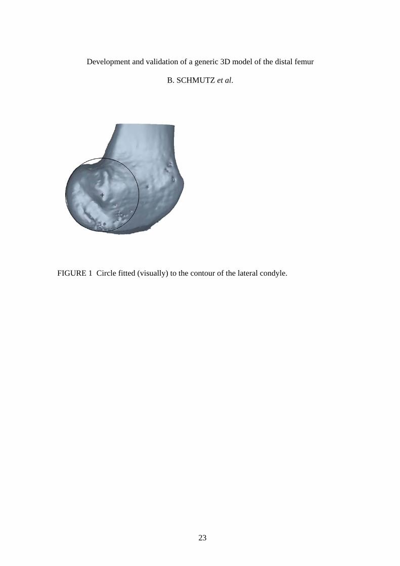
lateral/medial view (Fig. 1). A circle (of variable radius) was then visually fitted to the

profile of the condyle.

[Insert figure 1 about here]

The x-axis of the coordinate system was defined as the line passing through the

medial and lateral circle centres as seen in Figure 2. The midpoint between the circle

centres on the medial/lateral condyles was taken as the origin of the coordinate system.

The model was rotated about the x-axis until the diaphysial axis was parallel, in the yz-

plane, with the z-axis. The y-axis was orthogonal to both the x- and z-axes.


After alignment the models were scaled uniformly to the average condylar width

of the femur models. The circle centres on the medial and lateral condyles were taken as

6

measuring positions for determining the width of the femur. The distance between these

points does not necessarily correspond to the maximum width of the femur.

2.3 Repeatability study on the alignment method

A repeatability study was conducted to quantify the variability involved in aligning a

model with the common coordinate system. A randomly chosen model was aligned with

the coordinate system by following the method developed in this study. The following

values were recorded: the medial/lateral circle centres in data coordinates, the distance

between the circle centres on the medial/lateral condyles, and the angle through which

the model was rotated about the x-axis. The alignment was repeated five times with the

same model and the measurements were recorded. For each set of measurements the

average, standard deviation and worst case error were calculated.

2.4 Computerised re-sectioning of the models & contour extraction

The aligned and scaled models were computer graphically sectioned in planes

orthogonal to the z-axis. The models were sectioned at 1 mm intervals. The range on the

z-axis over which the models were sectioned spanned from 90 mm (proximal) to -28

mm (distal) generating 119 image slices for each model. The external bone contour was

automatically extracted from each image slice using a border tracing algorithm [17].

2.5 Combining and averaging of the extracted contours

7

In order to determine the average outline of the bone the extracted contours were

combined for each plane of section. Although the models have been aligned with a

common coordinate system, their contours in the shaft region when displayed together

were not closely superimposed as Figure 3a clearly shows.

[Insert figure 3a & 3c about here]

The most likely explanation for this lack of shaft alignment is due to differences

in the angle between the bone’s diaphysial axis and the line connecting the circle centres

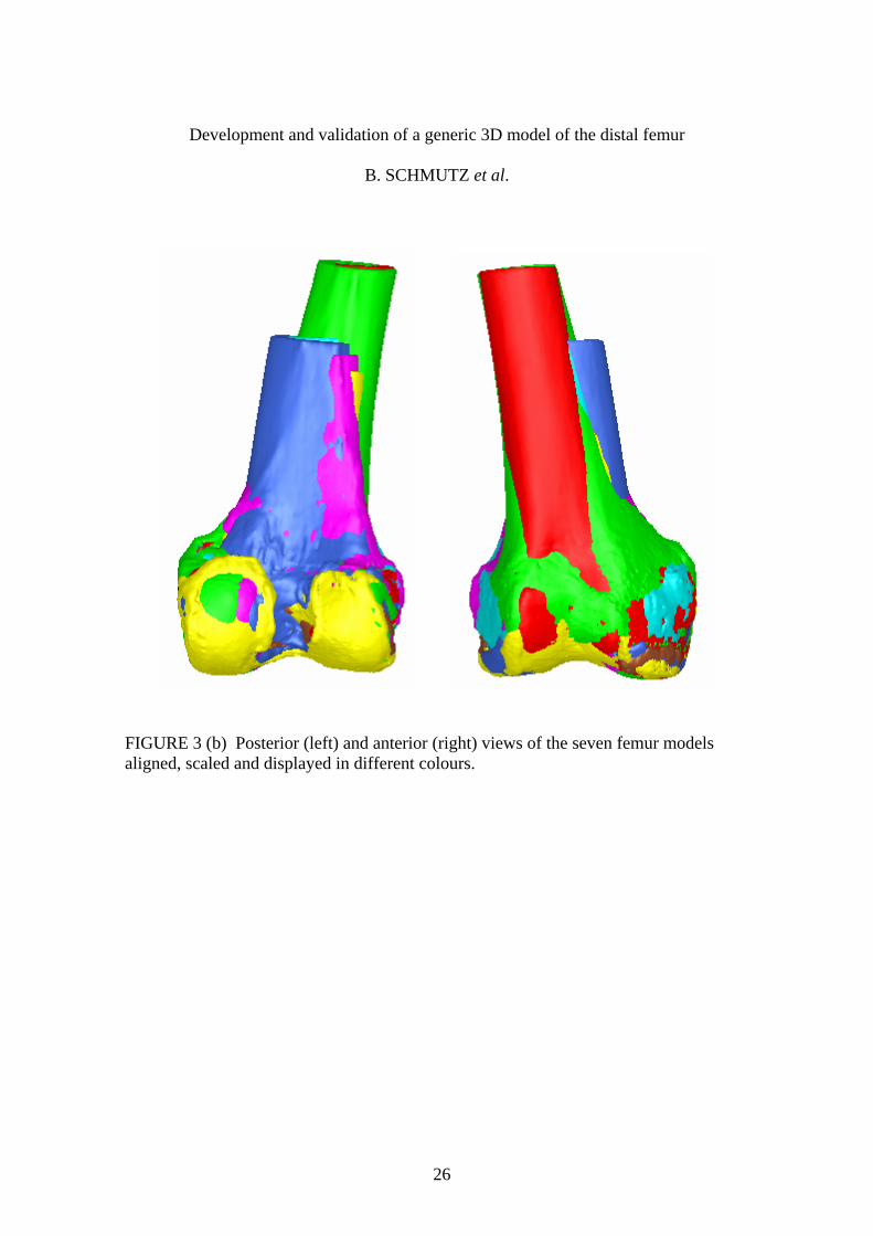
on the medial and lateral condyles (x-axis) as seen in Figure 3b.

To obtain a better alignment for the contours prior to averaging the contours

were translated such that their centroids were aligned at a common point (Fig. 3c). The

average of all the centroid positions was chosen as the common point for the alignment

of the contours. The average outline was determined by employing a graphical method

which lent itself to automation [15].

2.6 Reconstruction of the averaged contours

The generic 3D model was reconstructed from the average contour outlines by firstly

creating a volume (3D) array from the images of the average contour outlines. Then a

list of vertices and polygons describing the contour surface was generated. Finally, the

minimum amount of spatial smoothing was performed on the polygon mesh in order to

preserve the local morphology.

8

Due to the limited amount of image data it was necessary to take one femur

model (for validation) out of the data set of the available seven models and use the

remaining six for the development of the generic model. Using the approach of ‘take

one out’ removed any bias of the generic model towards the reference model since the

latter was excluded from the dataset used to generate the former. Furthermore, this

approach enabled using all seven CT image reconstructed models as reference models.

2.7 Validation of the generic model

The method used in this study to quantify the difference between two models was based

on calculating the disparity between the surface geometry of two models on a point to

point basis. The disparity function was based on Besl & McKay’s [18] Iterative Closest

Point (ICP) algorithm which calculates the Euclidean distance between a given point

and its nearest neighbour on a geometric entity. The definition of the disparity function

was adapted from Besl & McKay [18] and is presented in the appendix. The mean error

obtained by using Equation (3) is a measure of the overall similarity (disparity) between

two models. A low value indicates a high similarity whereas a high value indicates

greater disparity. The disadvantage of such an approach is that the error is non-

directional, i.e. it provides no reference to the location at which two models differ. To

provide some means of reducing the model space over which the error was calculated

the models were clipped proximally by a plane orthogonal to the z-axis and set at a

distance equal to half of the model’s condylar width away from the origin. In this way

the overall difference between the models in the condylar region could be quantified in

a way not affected by variations in the angle between the bone’s long axis and the line

9

connecting the circle centres on the medial and lateral condyles (x-axis) as seen in

Figure 3b. The mean error between the models was also calculated for the full length

(clipped at condylar width above origin) of the models.

Prior to quantifying the difference between a generic and a reference model the

generic model was scaled to the average (of three repeats) measurement of the condylar

width of the reference model. Then the two models were brought into optimal alignment.

The ‘gross’ alignment was achieved by aligning the models relative to the common

coordinate system. The alignment of the models was then iteratively ‘fine’ tuned by

transforming (translations and rotations) one model until the disparity function (Eqn. 2)

converged at a minimum.

The development and validation of the generic models was performed on a PC

(Pentium 4, 2.4 GHz, 512 MB RAM) using customised graphical user interfaces

developed in IDL 5.5 (Research Systems Inc, Boulder, USA).

3 Results

3.1 Repeatability of the alignment method

Repeatability of fitting circles to the medial/lateral profiles of the condyles was good,

the variation in the obtained circle coordinate positions being less than 1 mm (Table 1).

The y-component of the circle centres showed the greatest variability with a SD of 0.30

and 0.32 and a maximal difference between positions of 0.77 mm and 0.89 mm for the

lateral and the medial condyles, respectively.

10

[Insert table 1 about here]

The x-coordinates of the circle centres were fairly constant with a SD of 0.13

and 0.02, and a maximal difference between positions of 0.11 mm and 0.05 mm for the

lateral and the medial condyle, respectively. This was also reflected by the low variation

in the distance between the circle centres of 0.13 SD and 0.34 mm as the largest

difference in measurements which is equivalent to a percentage error of 0.4%. The

angle through which the model was rotated about the x-axis had a standard deviation of

0.11, with a relatively low maximum difference between the measurements of 0.26°.

3.2 Interspecimen variability

For a qualitative assessment of how and where the morphology of the femur models

differed, the models were aligned with the common coordinate system, scaled to the

average width of the data set and then displayed as different coloured polygon meshes

in the same view (Fig. 3b).

[Insert figure 3b about here]

The most obvious differences between the models are the variations in the angle

between the diaphysial axis and the axis joining the circle centres on the medial and

lateral condyles (x-axis). The differences in the condylar region appeared to be random

and relate to the local characteristic morphologies of the individual models. The

11

different lengths of the models are a result of scaling the individual models up or down

to the average width of the data set.

The largest interspecimen variability between the aligned contours was in the

order of 13 mm and caused by an osteophyte on the lateral aspect of the medial condyle.

The largest variability not caused by an osteophyte was 9 mm and occurred on the

anterior aspect of the medial condyle.

3.3 Resulting generic model

The generic model that has been developed from the data of seven femora is shown in

Figure 4.


3.4 Comparing reference models to the generic model

Error values between generic and femur models are provided for resection of the bone

shaft half the condylar width above the origin (Table 2) and full condylar width above

the origin (Table 3). Greatest maximum errors were recorded for femur 7 from an

individual with a groove on the anterior aspect of the condyles, whereas the greatest

mean errors were recorded from an individual with prominent osteophytes (femur 2).


12


4 Discussion

4.1 Repeatability study on the alignment of the models with the coordinate system

A repeatability study has demonstrated that the accuracy of the method for aligning the

reconstructed femur models with a common coordinate system prior to sectioning was

sufficient for the purpose of this project. The variations resulting from the alignment of

the model with the common coordinate system were either overshadowed by the

interspecimen variability of the bone contours, or were too small to have any noticeable

effect on the cross sectional dimension of the bone [15]. The only comparable study

[13] did not provide results regarding the repeatability of the alignment method used.

4.2 Resulting generic model

The developed generic model (Fig. 4) exhibits the characteristic shape of the distal

femur. The maximal interspecimen variability of 13 mm between the contours was

considerably higher than the 5 mm observed in the study by Siu et al. [13] who

considered that their five knees were representative of a ’normal‘ population. Studies by

Noble et al. [19,20] reported that the interspecimen variability in the morphology of

bones is increased by aging. The maximum variability in the bone contours in our study

was caused by an osteophyte on the lateral aspect of the medial condyle. Therefore, it is

most likely that the larger interspecimen variability of the knees used in this study was

13

due to the effect of aging as the average age of the knees was 20 years higher than that

in the study by Siu et al. [13].

By visual comparison, the generic model of this study contains more local

variations on the surface compared to Siu’s [13] model which is of smoother appearance.

This difference is most likely a combination of two factors: one is the narrower spacing

(0.5 mm compared to 3 mm in Siu’s [13] study) of the CT image slices; the other is the

minimal amount of smoothing performed on this model which was done in an effort to

preserve as much local surface detail as possible. Depending on the requirements of

future applications of the model further smoothing would be possible.

The model of the femur developed by Martelli et al. [10] based on the data of six

cadaveric knees can be considered as a reductionistic approach as the condyles were

represented by ellipsoids interconnected by a crossbar. Therefore, the visual appearance

of the generic model developed by Martelli significantly differs from the one presented

in this study. Comparison with other models [9,11,12] reported in the literature was not

conducted as those models were based on data sets of one to two femora.

The accuracy of the CT-based data acquisition method used in this study is

slightly lower compared to the methods used in similar studies [10-12]. However,

considering that the average outline of the combined contours was obtained it is

questionable whether a more accurate acquisition method would improve the result in

any meaningful way.

14

4.3 Comparing individual models to the generic models

There was a considerable spread in the average error values between the different femur

and generic models which ranged from 0.94 to 2.52 mm for the models that were

clipped at half of their condylar width (Table 2). For the longer models (clipped at their

condylar width) the average errors ranged from 0.99 to 2.52 mm (Table 3). As expected,

the average errors were lower for the models that did not display any bony outgrowths

(osteophytes) at the joint margins such as the models of femur 3, 5, 8 and 9. The highest

average errors of 2.19 and 2.52 mm were obtained for the two models (Femur 2 & 7)

that based on visual judgement, were excluded from the data set used to develop the

generic model. This indicates that the method of using the principle of ‘nearest

neighbour’ for quantifying the difference between two 3D models was in agreement

with the qualitative assessment of the models based on their visual appearance.

For the cases when the differences between the models with the longer shafts

were calculated the average error slightly decreased for two models (4 & 5) remained

the same for one (model 2) and slightly increased for six models. The greatest change of

0.05 mm in the average error was obtained for femur 3 and is equivalent to a 5%

increase of the value calculated for the shorter version of the model. This indicates that

although the variations in the angle between the diaphysial axis and the axis through the

condyles (x-axis of coordinate system) did affect the resulting average error, the extent

was not significant.

The minimum and maximum error values for both the short and the long

versions of the models did not appear to bear any relation to the average error, since

15

higher min/max values did not necessary result in higher average error values and vice

versa (see Table 2 & 3).

A visual comparison of the aligned models has shown that in no two cases were

the local morphological differences between a femur and generic model the same even

if the average error was similar such as for Femur 5 and Femur 9. This appears to be a

reflection of local morphological differences between individual bones.

Compared to studies involving CT image 3D reconstructions, the average errors

between generic and individual models of the femur are comparable to the higher end of

the range [21-24] of errors reported in the literature. This indicates that the generic

model developed in this study represents the morphology of a particular femur (from the

available dataset) reasonably well. Provided that the particular femur is considered

normal, i.e. does not contain a significant number of osteophytes or any other

deformities. However, it is important to note that the generic models used in this study

were both generated and validated based on image data from older specimens (average

age 80 years). Therefore, it is not known how representative the developed generic

model would be of a particular femur model generated from a younger (55 years)

subject.

In relation to the potential clinical relevance of the method of quantifying the

difference between two 3D models, osteophytes are routinely assessed visually with

regard to small, moderate or large size but do not necessarily relate strongly to clinical

symptoms as their size is only one of the features of degenerative joint disease. Thus, it

is not likely that the developed method of comparing two 3D models will be applied in

this particular clinical setting. Other potential clinical applications have not yet been

identified.

16

5 Conclusion

In this study, computer graphical methods were developed for the construction of a

generic 3D model of the distal femur based on CT-scan image data.

The advantage of this method of generating a generic model over other methods

[9-13] is that no specimens have to be dissected since the 3D data of the joint can be

acquired using standard CT imaging without the need for a calibration frame.

Furthermore, although more expensive than CT, MR (magnetic resonance imaging)

could potentially be used for the acquisition of data from patients/subjects without

exposing them to medically unjustified radiation. This method is therefore very

appealing as a technique applicable to the future development of generic models based

on larger and more age diverse data sets.

The resulting generic 3D model contained more local variations in the surface of

the condylar region compared to Siu’s [13] model which is most likely the result of

different imaging and reconstruction parameters used in this study. The general

morphology of the two models is comparable.

The differences between the generic model and a particular model of the femur

was quantified by means of an average error metric which was based on calculating the

Euclidean distances from points on the surface of one model to their nearest neighbours

on the other model. The considerable range of 0.99 - 2.5 mm in the obtained average

error values appears to be a reflection of the degree of bony outgrowths at the joint

margins of some models, since all the models with no outgrowths had lower error

values. This indicates that the method of using the principle of ‘nearest neighbour’ for

17

quantifying the difference between two 3D models was in agreement with the

qualitative assessment of the models based on their visual appearance.

The generic model represents the morphology of a particular femur (from the

available dataset) reasonably well, provided that the particular femur is considered

normal. Due to the limited and aged data set further studies will be required to develop a

generic model which is representative of a larger population sample.

Acknowledgement

The authors wish to thank the Department of Medical Imaging, Flinders Medical Centre,

for the CT scan images; the Department of Anatomy & Histology of the School of

Medicine, Flinders University for providing the cadaver specimens.

Appendix

The Euclidean distance d(p1, p2) between two points p1 = (x1 ,y1, z1) and p2 = (x2 ,y2, z2)

is d(p1, p2) = || p1 - p2 ||. Let A be the point set of vertex coordinates (x, y, z) of the

generic model denoted as A = {ai} for i = 1, ..., n. Let B be the point set of vertex

coordinates of the femur model denoted as B = {bj} for j = 1, ..., m. Then the minimum

Euclidean distance from point bj on the femur model to its closest neighbour ai on the

generic model is given by

( )}{( )ijnij abdAbd ,min,

,...,1min ∈= . (1)

18

The disparity function (D) is then defined as the sum of all the distance values from

every point (vertex) on the femur model (set B) to the closest point on the generic model

(set A), which can be written as:

. (2) (∑=

=m

jj AbdD

0min , )

To provide a more meaningful comparison between the models the average error

appeared to be more appropriate than the total error, since not all models had the same

number of vertices. Therefore, the sum in Equation (2) was divided by the number of

points in the vertex data set of the femur model to obtain the mean error (ME) as

follows

(∑=

=m

jj Abd

mME

0min ,1 ) . (3)

References

[1] Leyvraz PF. & Rakotomanana L., 2000, The anatomy and function of the knee –

The quest for the Holy Grail? The Journal of Bone & Joint Surgery, 82-B(8):

1093-1094.

[2] Pinskerova V., Maquet P. & Freeman MAR., 2000, Writings on the knee between

1836 and 1917. The Journal of Bone & Joint Surgery, 82-B(8):1100-1102.

19

[3] Wetz HH. & Jacob HAC., 2001, Funktionelle Anatomie und Kinematik des

Femurotibialgelenks: Forschungsergebnisse von 1836-1950. Der Orthopäde, 30:

135-144.

[4] Pinskerova V., Iwaki H. & Freeman MAR., 2000, The shapes and relative

movements of the femur and tibia at the knee. Der Orthopäde, 29(Suppl. 1): 3-5.

[5] Eckhoff DG., Bach JM., Spitzer VM. & Reinig KD., 2003, Three-dimensional

morphology and kinematics of the distal part of the femur viewed in virtual reality:

Part II. The Journal of Bone & Joint Surgery, 85-A(Suppl. 4): 97-104.

[6] Huson A., 1974, Biomechanische Probleme des Kniegelenks. Der Orthopäde, 3:

119-126.

[7] Kurosawa H., Walker PS., Abe S., Garg A. & Hunter T., 1985, Geometry and

motion of the knee for implant and orthotic design. Journal of Biomechanics,

18(7): 487-499.

[8] Noble P., Gordon M., Weiss J., Reddix R., Conditt M. & Mathis K. 2005, Does

total knee replacement restore normalknee function? Clinical Orthopaedics and

Related Research, 431:157-165.

[9] Wismans J., Veldpaus F., Janssen J., Huson A. and Struben P., 1980. A three-

dimensional mathematical model of the knee-joint. Journal of Biomechanics,

13(8): 677-685.

[10] Martelli S., Acquaroli F, Pinskerova V, Spettol A., & Visani A., 2002, An

Anatomical Model of the Knee Joint Obtained by Computer Dissection. In Dohi T.

& Kikinis R. (Eds.) Lecture Notes in Computer Science: Vol. 2489. Proceedings of

V MICCAI 2002, Tokyo, Sept. 23-28, 2002, (pp. 308-314), Springer, Berlin.

20

[11] Ghosh SK. 1983, A close-range photogrammetric system for 3-D measurements

and perspective diagramming in biomechanics. Journal of Biomechanics, 16(8):

667-674.

[12] Huiskes R., Kremers J., de Lange A., Woltring HJ., Selvik G. and van Rens Th.JG.

1985, Analytical stereophotogrammetric determination of three-dimensional knee-

joint geometry. Journal of Biomechanics, 18(8): 559-570.

[13] Siu D., Rudan J., Wevers HW. & Griffiths P., 1996, Femoral Articular Shape and

Geometry: A three-dimensional computerised analysis of the Knee. The Journal of

Arthroplasty, 11(2): 166-173.

[14] Rubin PJ., Leyvraz PF., Aubaniac JM., Argenson JN., Esteve P. & DeRoguin B.,

1992, The Morphology of the Proximal Femur: A Three-Dimensional

Radiographic Analysis. The Journal of Bone & Joint Surgery, 74-B: 28-32.

[15] Schmutz B., 2005, From planar radiographs to 3D models: Reconstruction of the

distal femur. PhD Thesis, Faculty of Science & Engineering, Flinders University,

South Australia.

[16] Kwak SD., Blankevoort L., Ahmad CS., Gardner TR., Grelsamer RP., Henry JH.,

Ateshian GA. & Mow VC., 1995, An anatomically based 3D coordinate system

for the knee joint. Adv. Bioeng. ASME, BED-31: 309-310.

[17] Fanning DW., 2002, FIND_BOUNDARY. [Computer program]. Available URL:

http://www.dfanning.com/programs/find_boundary.pro (accessed 5 June 2003)

[18] Besl PJ. & McKay ND., 1992, A Method for Registration of 3-D Shapes. IEEE

Transaction on Pattern Analysis and Machine Intelligence, 14(2): 239-256.

21

http://www.dfanning.com/programs/find_boundary.pro

[19] Noble PC., Alexander JW., Lindahl LJ., Yew DT., Granberry WM. & Tullos HS.,

1988, The anatomic basis of femoral component design. Clinical Orthopaedics,

235: 148–165.

[20] Noble PC., Box GG., Kamaric E., Fink MJ., Alexander JW. & Tullos HS., 1995,

The effect of aging on the shape of the proximal femur. Clinical Orthopaedics,

316: 31–44.

[21] Robertson DD., Yuan J., Bigliani LU., Flatow EL. & Yamaguchi K., 2000, Three-

Dimensional Analysis of the Proximal Part of the Humerus: Relevance to

Arthroplasty. Journal of Bone and Joint Surgery, 82-A(11): 1594-1602.

[22] Rubin PJ., Leyvraz PF., Aubaniac JM., Argenson JN., Esteve P. & DeRoguin B.,

1992, The Morphology of the Proximal Femur: A Three-Dimensional

Radiographic Analysis. The Journal of Bone & Joint Surgery, 74-B: 28-32.

[23] Aubin CE., Dansereau J., Parent F., Labelle H. & DeGuise JA., 1997,

Morphometric evaluations of personalised 3D reconstructions and geometric

models of the human spine. Medical & Biological Engineering & Computing,

November: 611-618.

[24] Nagashima M., Inoue K., Sasaki T., Miyasaka K., Matsumura G. & Kodama G.,

1998, Three-Dimensional Imaging and Osteometry of Adult Human Skulls using

Helical Computed Tomography. Surg Radiol Anat., 20: 291-297.

22

Development and validation of a generic 3D model of the distal femur

B. SCHMUTZ et al.

FIGURE 1 Circle fitted (visually) to the contour of the lateral condyle.

23


B. SCHMUTZ et al.

FIGURE 2 Femur model aligned with the coordinate system.

24


B. SCHMUTZ et al.

FIGURE 3 (a) Combined contours of aligned models. (c) Contours aligned with the average of their centroids (average contour in bold).

25


B. SCHMUTZ et al.

FIGURE 3 (b) Posterior (left) and anterior (right) views of the seven femur models aligned, scaled and displayed in different colours.

26


B. SCHMUTZ et al.

FIGURE 4 Posterior (left) and anterior (right) views of the generic model generated from the averaged contour data of seven femora.

27


B. SCHMUTZ et al. TABLE 1 Tabulated results of the repeatability study for alignment of a randomly chosen model with the common coordinate system.

L )ateral Circle Centre (mm Medial Circle Centre (mm) Distance Angle x z x y z (m ) (Deg)

- 8 8 -3 0 4 5 1 0 -4 0 y m

44.6 8.0 8.8 2.6 2.6 4.1 87.60 3.84 -44.61 8.23 -38.93 42.66 12.59 -44.06 87.53 3.77 -44.69 7.98 -38.83 42.61 12.64 -44.28 87.60 4.00 -44.94 7.46 -38.43 42.60 12.26 -44.30 87.87 3.75

-44.72 7.76 -38.90 42.62 13.14 -44.18 87.67 3.95 Average -44.73 7.90 -38.78 42.63 12.65 -44.18 87.65 3.86 SD 0.13 0.30 0.20 0.02 0.32 0.11 0.13 0.11 Max Error 0.11 0.77 0.49 0.05 0.89 0.24 0.34 0.26

28


B. SCHMUTZ et al. TABLE 2 Table of error values between femur models and generic models for which the bone shaft was resected at a distance equal to half of their condylar width above the origin.

Femur No.

min Error (mm)

max Error (mm)

mean Error (mm)

1 0.05 5.83 1.502 0.06 8.30 2.523 0.04 3.92 0.944 0.04 9.82 1.765 0.06 4.33 1.186 0.06 7.21 1.467 0.04 10.49 2.198 0.04 5.43 1.349 0.05 3.83 1.11

29


B. SCHMUTZ et al. TABLE 3 Table of error values between femur models and generic models for which the bone shaft was resected at a distance equal to their condylar width above the origin.

Femur No.

min Error (mm)

max Error (mm)

mean Error (mm)

1 0.07 6.09 1.542 0.07 8.55 2.523 0.02 4.29 0.994 0.04 9.64 1.745 0.04 4.37 1.176 0.04 7.73 1.497 0.07 10.43 2.218 0.08 5.45 1.369 0.05 3.95 1.14

30


B. SCHMUTZ et al. List of figure captions:

FIGURE 1 Circle fitted (visually) to the contour of the lateral condyle.

FIGURE 2 Femur model aligned with the coordinate system.

FIGURE 3 (a) Combined contours of aligned models. (c) Contours aligned with the average of their centroids (average contour in bold). FIGURE 3 (b) Posterior (left) and anterior (right) views of the seven femur models aligned, scaled and displayed in different colours. FIGURE 4 Posterior (left) and anterior (right) views of the generic model generated from the averaged contour data of seven femora.

31

development and validation of a generic 3d model of the ...eprints.qut.edu.au/5636/1/5636.pdf ·...

Documents