development and thermal management of a dynamically

Wright State University Wright State University

CORE Scholar CORE Scholar

Browse all Theses and Dissertations Theses and Dissertations

2018

Development and Thermal Management of a Dynamically Development and Thermal Management of a Dynamically

Efficient, Transient High Energy Pulse System Model Efficient, Transient High Energy Pulse System Model

Nathaniel J. Butt Wright State University

Follow this and additional works at: https://corescholar.libraries.wright.edu/etd_all

Part of the Mechanical Engineering Commons

Repository Citation Repository Citation Butt, Nathaniel J., "Development and Thermal Management of a Dynamically Efficient, Transient High Energy Pulse System Model" (2018). Browse all Theses and Dissertations. 1975. https://corescholar.libraries.wright.edu/etd_all/1975

This Thesis is brought to you for free and open access by the Theses and Dissertations at CORE Scholar. It has been accepted for inclusion in Browse all Theses and Dissertations by an authorized administrator of CORE Scholar. For more information, please contact [email protected].

https://corescholar.libraries.wright.edu/

https://corescholar.libraries.wright.edu/etd_all

https://corescholar.libraries.wright.edu/etd_comm

https://corescholar.libraries.wright.edu/etd_all?utm_source=corescholar.libraries.wright.edu%2Fetd_all%2F1975&utm_medium=PDF&utm_campaign=PDFCoverPages

http://network.bepress.com/hgg/discipline/293?utm_source=corescholar.libraries.wright.edu%2Fetd_all%2F1975&utm_medium=PDF&utm_campaign=PDFCoverPages

https://corescholar.libraries.wright.edu/etd_all/1975?utm_source=corescholar.libraries.wright.edu%2Fetd_all%2F1975&utm_medium=PDF&utm_campaign=PDFCoverPages

mailto:[email protected]

Development and Thermal Management of a Dynamically Efficient, Transient High Energy Pulse System Model

A thesis submitted in partial fulfillment of the requirements for the degree of Master of Science in Mechanical Engineering

By:

Nathaniel J. Butt B.S.M.E., Ohio Northern University, 2016

2018 Wright State University

Distribution Statement A: Unlimited Distribution

Cleared for Public Release by AFRL/WS Public Affairs on 07 MAY 2018

Case Number 88ABW-2018-2220

The views expressed in this article are those of the author and do not reflect the official policy or

position of the United States Air Force, Department of Defense, or the U.S. Government.

WRIGHT STATE UNIVERSITY

GRADUATE SCHOOL

April 25, 2018

I HEREBY RECOMMEND THAT THE THESIS PREPARED UNDER MY SUPERVISION BY Nathaniel J. Butt ENTITLED Development and Thermal Management of a Dynamically Efficient, Transient High Energy Pulse System Model BE ACCEPTED IN PARTIAL FULFILLMENT OF THE REQUIREMENTS FOR THE DEGREE OF Master of Science in Mechanical Engineering.

Rory Roberts, Ph.D.

Thesis Director

Rory Roberts, Ph.D.

Zifeng Yang, Ph.D.

Committee on Final Examination

Barry Milligan, Ph.D.

Interim Dean of the Graduate School

Mitch Wolff, Ph.D. Joseph C. Slater, Ph.D., P.E.

Chair, Department of Mechanical and

Materials Engineering

WRIGHT STATE UNIVERSITY

iv

Abstract:

Butt, Nathaniel J., M.S.M.E Department of Mechanical and Materials Engineering, Wright State

University, 2018. Development and Thermal Management of a Dynamically Efficient, Transient

High Energy Pulse System Model

As technology advances, the abilities of civilian and military vehicles, both air and ground, will

undoubtedly increase as well. One of the main areas of improvement is in the electronics area.

The new electronics are ever smaller, use ever higher amounts of electrical power, and require

ever smaller temperature tolerances. This leads to the problem of effectively managing the

increasing thermal loads and temperature tolerances on these systems. One electronic system

that causes concern is a high energy pulse system (HEPS). These devices have very high thermal

loads (100s of kW). On an air vehicle, where thermal management by legacy methods (i.e. fuel

as the heat sink) is already problematic, a HEPS will certainly overload the thermal management

system (TMS). HEPS performance must be understood and quantified more accurately to

understand the design requirements of a TMS for this device. To aid in this understanding, the

HEPS itself and a palletized system to thermally manage the HEPS will be modeled.

Previous analysis of a cryogenic palletized HEPS contained a simplified power model for a HEPS

that had a set efficiency and always gave a certain amount of optical power out and a certain

amount of power dissipated as heat based on that set efficiency. The HEPS model developed

and presented takes into account the temperature of internal HEPS components and changes

the efficiency accordingly. The HEPS efficiency changes with component temperature to

v

provide a better understanding of the consequences of not thermally managing a HEPS

effectively.

Along with the HEPS model, a cryogenic-based palletized TMS using Liquefied Natural Gas (LNG)

for indirectly cooling the HEPS was modeled. Using LNG as a method of cooling is a possible

alternative to using very large legacy systems (fuel as heat sink) to cool a HEPS. The architecture

of this palletized system uses LNG to cool the heat loads. The LNG then becomes the fuel for

the turbo-generator, which produces electrical power for the HEPS and other pallet systems.

The main reason for modeling a palletized system like this is to provide a platform to conduct a

comparison test between a constant efficiency HEPS model and a dynamic efficiency HEPS

model. This will show whether or not the dynamic efficiency aspects of HEPS operation must be

taken into account when designing the coupled TMS architecture. Learning the nuances of HEPS

component operation and how the component efficiencies change with temperature will pave

the way for future work in designing a TMS capable of keeping these HEPS component

temperatures in perfect balance, thus providing a robust, usable, and practical HEPS design.

vi

Table of Contents:

Introduction: .............................................................................................................................................. 1

Problem Overview: ................................................................................................................................... 1

Proposed Solution for HEPS Modeling: ..................................................................................................... 3

Palletized System Modeling: ..................................................................................................................... 7

Literature Review: .................................................................................................................................... 8

Previous HEPS Modeling Coupled with a Thermal Management System: ............................................... 8

Cryogenic Palletized HEPS with LNG: ...................................................................................................... 10

HEPS Internal Component Modeling: ..................................................................................................... 11

Exploratory Research and Study:......................................................................................................... 13

Background on Fiber Lasers: ................................................................................................................... 13

Modeling the Laser Beam: ...................................................................................................................... 15

Laser Diode Parameters: ......................................................................................................................... 16

Laser Diode Packaging: ........................................................................................................................... 18

HEPS Efficiency Definitions: .................................................................................................................... 21

Models Created in MATLAB/Simulink: ............................................................................................... 21

Temperature Sensitive HEPS Model: ...................................................................................................... 22

HEPS Cooling Loop: ................................................................................................................................. 27

Model Testing: ........................................................................................................................................ 31

Cryogenic Palletized System Model: ....................................................................................................... 37

Results and Discussion: ......................................................................................................................... 38

Test Stand with Water/Ethylene-Glycol Coolant: ................................................................................... 40

Test Stand with Cold Natural Gas Coolant: ............................................................................................. 50

Test Stand Results Discussion: ................................................................................................................ 59

Palletized System with Water/Ethylene-Glycol Coolant: ........................................................................ 60

Conclusions: ............................................................................................................................................. 74

References: ............................................................................................................................................... 78

vii

Table of Figures: Figure 1: Growth of Software Complexity in Aerospace Systems1 ............................................................... 1

Figure 2: Power and Thermal Requirements for Fighter Aircraft2 ................................................................ 2

Figure 3: Bohr Model and Energy Levels4 ..................................................................................................... 4

Figure 4: Two Methods of Pumping Solid State Lasers6 ............................................................................... 5

Figure 5: Fiber Laser Setup6 .......................................................................................................................... 5

Figure 6: Cladding Pumped Fiber Laser Example6 ......................................................................................... 6

Figure 7: Palletized System Achitecture by Nuzum3 ..................................................................................... 7

Figure 8: Palletized System Mission 1 Profile3 ............................................................................................ 11

Figure 9: Components of a HEPS with a SSL9 .............................................................................................. 12

Figure 10: Simple Fiber Laser Diagram showing Core and Cladding13 ........................................................ 14

Figure 11: Power Evolution of Ultrafast Fiber Lasers13 ............................................................................... 15

Figure 12: Diagram Showing Basics of Gaussian Curve Model for Laser Diode Output ............................. 16

Figure 13: Threshold Current vs. Optical Output Power of a Laser Diode19 ............................................... 18

Figure 14: Laser Diode Array Packaging Diagram ....................................................................................... 19

Figure 15: Laser Diode Modules Diagram, Array Size (4 x 4) ...................................................................... 20

Figure 16: HEPS Cooling Loop Model Diagram ........................................................................................... 28

Figure 17: Heat Exchanger With Energy Flow in and out of Each Discrete Volume23 ................................ 29

Figure 18: Plate Fin Configuration HX Geometry (fins serrated to promote turbulence)23 ........................ 30

Figure 19: Heat Plate Surface and Diode Stack Representation ................................................................. 30

Figure 20: Simulink Block Diagram of Heat Plates for Three Major HEPS Components ............................. 31

Figure 21: Laser Diode and Gain Medium Output (Diodes at Reference Temperature, 12°C) .................. 33

Figure 22: Laser Diode and Gain Medium Output (Diodes from 12°C to 22°C) ......................................... 34



Figure 25: Palletized TMS Architecture Diagram25 ..................................................................................... 37

Figure 26: Activation Profile for Test Stand HEPS Activation...................................................................... 41

Figure 27: Test Stand Configuration for Water/Ethylene-Glycol Cooling Fluid .......................................... 42

Figure 28: Optical Power of Laser Diode Configurations Cooled with Water/Ethylene-Glycol (Full and

Zoomed View, Heat Plate Thickness = 10mm) ............................................................................................ 42

Figure 29: Optical Power During HEPS Activation Cooled with Water/Ethylene-Glycol for Heat Plate

Thicknesses (10, 20, and 50 mm) ................................................................................................................ 43

Figure 30: Effective Efficiency during HEPS Activation Cooled with Water/Ethylene-Glycol for Heat Plate

Thicknesses (10, 20, and 50 mm) ................................................................................................................ 44

Figure 31: Re, h, and Laser Diode Stack Temperature Values for the (25x1) Array with a Heat Plate

Thickness = 10 mm ...................................................................................................................................... 46


Thickness = 10 mm ...................................................................................................................................... 47


Thickness = 10 mm ...................................................................................................................................... 48

viii

Figure 34: Water/Ethylene-Glycol In and Out Temperatures for the Three Diode Configuraitons with a

Heat Plate Thickness = 10 mm .................................................................................................................... 49

Figure 35: Test Stand Configuration for Cold Natural Gas Cooling Fluid .................................................... 51

Figure 36: Optical Power of Laser Diode Configurations Cooled with CNG (Full and Zoomed View, Heat

Plate Thickness = 10mm) ............................................................................................................................ 51

Figure 37: Optical Power During HEPS Activation Cooled with CNG for Heat Plate Thicknesses (10, 20,

and 50 mm) ................................................................................................................................................. 52

Figure 38: Effective Efficiency during HEPS Activation Cooled with CNG for Heat Plate Thicknesses (10,

20, and 50 mm) ........................................................................................................................................... 53


Thickness = 10 mm ...................................................................................................................................... 55


Thickness = 10 mm ...................................................................................................................................... 56


Thickness = 10 mm ...................................................................................................................................... 57

Figure 42: CNG In and Out Temperatures for the Three Diode Configuraitons with a Heat Plate Thickness

= 10 mm ...................................................................................................................................................... 58

Figure 43: Activation Profile for Palletized HEPS Simulations .................................................................... 61

Figure 44: Optical Power out of Constant Efficiency HEPS for Palletized TMS Simulation ........................ 62

Figure 45: Thermal and Electrical Power of Constant Efficiency HEPS for Palletized TMS Simulation ...... 63

Figure 46: Cold Tank Parameters of Constant Efficiency HEPS for Palletized TMS Simulation .................. 63

Figure 47: Hot Tank Parameters of Constant Efficiency HEPS for Palletized TMS Simulation.................... 64

Figure 48: Tank Temperatures of Constant Efficiency HEPS for Palletized TMS Simulation ...................... 65

Figure 49: Optical Power out of Dynamic Efficiency HEPS for Palletized TMS Simulation ......................... 66

Figure 50: Thermal and Electrical Power of Dynamic Efficiency HEPS for Palletized TMS Simulation ....... 67

Figure 51: Cold Tank Parameters of Dynamic Efficiency HEPS for Palletized TMS Simulation ................... 68

Figure 52: Hot Tank Parameters of Dynamic Efficiency HEPS for Palletized TMS Simulation .................... 68

Figure 53: Tank Temperatures of Dynamic Efficiency HEPS for Palletized TMS Simulation ....................... 69

Figure 54: Laser Diode Temperatures of Dynamic Efficiency HEPS for Palletized TMS Simulation............ 70

Figure 55: Reynolds Numbers of Dynamic Efficiency HEPS for Palletized TMS Simulation ........................ 71

Figure 56: Heat Transfer Coefficients of Dynamic Efficiency HEPS for Palletized TMS Simulation ............ 71

ix

Table of Tables: Table 1: HEPS Component Efficiencies9 ...................................................................................................... 12

Table 2: Important Laser Diode Characteristics .......................................................................................... 17

Table 3: HEPS Parameters Initially Defined ................................................................................................ 23

Table 4: HEPS Model Initial Testing Parameter Values ............................................................................... 32

Table 5: HEPS Model Parameter Values for Model Simulation .................................................................. 39

Table 6: Laser Diode Packaging Parameters Defined ................................................................................. 40

Table 7: Water/Ethylene-Glycol Test Stand Parameters ............................................................................ 41

Table 8: Energy Output of HEPS for Each Laser Diode Configuration and Heat Plate Thickness with

Configurations Ranked Best to Worst (Water/Ethylene-Glycol) ................................................................ 45

Table 9: CNG Test Stand Parameters .......................................................................................................... 50


Configurations Ranked Best to Worst (CNG) .............................................................................................. 54

Table 11: HEPS Component Efficiencies and Values for Constant Efficiency Simulation ........................... 61

Table 12: Water/Ethylene-Glycol (60%) Physical Properties at 287K and 298K ......................................... 72

Table 13: Water Physical Properties at 287K and 298K .............................................................................. 72

x

Nomenclature (Text):

AFRL = Air Force Research Laboratories AIAA = American Institute of Aeronautics and Astronautics APTMS = Adaptive Power and Thermal Management System AVS = Air Vehicle System CNG = Cold Natural Gas FTMS = Fuel Thermal Management System FWHM = Full Width Half Maximum h = Heat transfer coefficient (W/m2 K) HELLADS = High Energy Liquid Laser Area Defense System HEPS = High Energy Pulsed System LNG = Liquefied Natural Gas PAO = Polyalphaolefin Oil Re = Reynold’s Number SLOC = Software Lines of Code SSL = Solid State Laser TMS = Thermal Management System

Nomenclature (Equations):

𝐴𝑣𝑎𝑙𝑢𝑒 𝐿𝐷 = A Value for Laser Diode Stack Gaussian Profile (peak @ center wavelength)

𝐴𝑏𝑠𝑜𝑟𝑝𝑡𝑖𝑜𝑛 𝐶𝑢𝑟𝑣𝑒𝐺𝑀 = Gain Medium Efficiency Absorption Profile (Gaussian Curve) 𝐴𝑏𝑠𝑜𝑟𝑝𝑡𝑖𝑜𝑛 𝑃𝑜𝑤𝑒𝑟𝐺𝑀 = Multiply Input Laser Diode Power across all Wavelengths by the Gain

Medium Absorption Curve, this yields the actual gain medium absorption curve

𝐶𝑣𝑎𝑙𝑢𝑒 𝐿𝐷 = C Value for Laser Diode Gaussian Profile (spectral width) 𝐶𝑣𝑎𝑙𝑢𝑒 𝐺𝑚 = C value for Gain Medium Gaussian Profile

𝐺𝑎𝑢𝑠𝑠𝑖𝑎𝑛𝑎𝑙𝑙 𝑠𝑡𝑎𝑐𝑘𝑠 = Gaussian Curve for all Stack Profiles added together to form one curve 𝐺𝑎𝑢𝑠𝑠𝑖𝑎𝑛𝐿𝐷 𝑠𝑡𝑎𝑐𝑘(𝑥) = Actual Gaussian Curve for one Stack Profile, x from 1 to 𝑁𝑈𝑀𝐿𝐷 𝑠𝑡𝑎𝑐𝑘𝑠

𝐼𝐻𝐸𝑃𝑆 = Current to HEPS (Amps) 𝐼𝑚𝑎𝑥 = Max Current per Laser Diode (Amps) 𝐼𝑡ℎ = Threshold Current (Amps)

𝐿𝐷𝐻𝑃,𝑎𝑟𝑒𝑎 = Laser diode heat plate surface area (m2) 𝐿𝐷𝐻𝑃,𝑙𝑒𝑛𝑔𝑡ℎ = Laser diode heat plate length (flow direction) (m)

𝐿𝐷𝐻𝑃,𝑡ℎ𝑖𝑐𝑘𝑛𝑒𝑠𝑠 = Laser diode heat plate thickness (mm) 𝑁𝑈𝑀𝐷𝑖𝑜𝑑𝑒𝑠 = Total Number of Laser Diodes Required for 𝑃𝑜𝑤𝑒𝑟𝑜𝑝𝑡𝑖𝑐𝑎𝑙

𝑁𝑈𝑀𝐿𝐷/𝑠𝑡𝑎𝑐𝑘 = Number of Laser Diodes per Stack (diodes in parallel) 𝑁𝑈𝑀𝐿𝐷 𝑠𝑡𝑎𝑐𝑘𝑠 = Number of Laser Diode Stacks (diodes in series) 𝑁𝑈𝑀𝑀𝑜𝑑𝑢𝑙𝑒𝑠 = Number of Laser Diode Array Modules 𝑃𝑜𝑤𝑒𝑟𝑜𝑝𝑡𝑖𝑐𝑎𝑙 = HEPS Design Optical Power from Laser Diodes (W)

𝑃𝑜𝑤𝑒𝑟𝑜𝑝𝑡𝑖𝑐𝑎𝑙 𝐴𝑆𝐸 = Total optical power out of aperture sharing element 𝑃𝑜𝑤𝑒𝑟𝑜𝑝𝑡𝑖𝑐𝑎𝑙 𝐵𝐷 = Total optical power out of beam director 𝑃𝑜𝑤𝑒𝑟𝑜𝑝𝑡𝑖𝑐𝑎𝑙 𝐺𝑀 = Total optical power out of gain medium

xi

𝑃𝑜𝑤𝑒𝑟𝑜𝑝𝑡𝑖𝑐𝑎𝑙 𝐿𝐷 = Total optical power out of all laser diodes, area under 𝐺𝑎𝑢𝑠𝑠𝑖𝑎𝑛𝑎𝑙𝑙 𝑠𝑡𝑎𝑐𝑘𝑠 𝑃𝑜𝑤𝑒𝑟𝑜𝑝𝑡𝑖𝑐𝑎𝑙 𝑀𝑅 = Total optical power out of training mirrors 𝑃𝑜𝑤𝑒𝑟𝑝𝑒𝑟 𝐿𝐷,𝑒𝑙𝑒𝑐 = Electrical Power per Laser Diode (W) 𝑃𝑜𝑤𝑒𝑟𝑝𝑒𝑟 𝐿𝐷,𝑜𝑝𝑡 = Nominal Optical Power per Laser Diode at 𝜆𝑐𝑒𝑛𝑡𝑒𝑟 𝐿𝐷 (W)

𝑃𝑜𝑤𝑒𝑟𝑝𝑒𝑟 𝐿𝐷𝑠𝑡𝑎𝑐𝑘 = Power per Laser Diode Stack (W) 𝑃𝑜𝑤𝑒𝑟𝑟𝑜𝑙𝑙𝑜𝑣𝑒𝑟 = Rollover Power in terms of Design Optical Output Power

𝑃𝑜𝑤𝑒𝑟𝑤𝑎𝑙𝑙 𝑝𝑙𝑢𝑔 = HEPS Wall Plug Power (W) 𝑃𝑜𝑤𝑒𝑟 𝑂𝑢𝑡𝑜𝑝𝑡𝑖𝑐𝑎𝑙,𝑚𝑎𝑥 = Max Possible Optical Power out of HEPS

𝑅𝑜𝑙𝑙𝑜𝑣𝑒𝑟𝑐𝑜𝑒𝑓𝑓 = Coefficient for Laser Diode Rollover Power 𝑇𝑖𝑛 𝐿𝐷 = Temperature of Coolant Fluid into Laser Diode (K)

𝑇𝐿𝐷(𝑥) = Laser Diode Stack Temperatures, x from 1 to 𝑁𝑈𝑀𝐿𝐷 𝑠𝑡𝑎𝑐𝑘𝑠 (K) 𝑇𝑜𝑢𝑡 𝐿𝐷 = Temperature of Coolant Fluid out of Laser Diode (K) 𝑇𝑟𝑒𝑓 𝐿𝐷 = Reference Temperature for Laser Diode Characteristics (K) 𝑉𝑓𝑤𝑑 = Laser Diode Forward Voltage Drop per Stack 𝑉𝐻𝐸𝑃𝑆 = Voltage to HEPS (Volts)

𝑉𝑝𝑒𝑟 𝐿𝐷 = Voltage per Laser Diode (Volts) 𝜆𝑐𝑒𝑛𝑡𝑒𝑟 𝐺𝑀 = Nominal Center Wavelength of Gain Medium Absorption Spectrum (m) 𝜆𝑐𝑒𝑛𝑡𝑒𝑟 𝐿𝐷 = Nominal Center Wavelength of Laser Diode Output at 𝑇𝑟𝑒𝑓 𝐿𝐷 (m)

𝜆𝑐𝑒𝑛𝑡𝑒𝑟 𝐿𝐷(𝑥) = Center Wavelength of each Stack (x should go from 1 to 𝑁𝑈𝑀𝐿𝐷 𝑠𝑡𝑎𝑐𝑘𝑠)(m) 𝜆𝑓𝑤ℎ𝑚 𝐺𝑀 = Full Width Half Maximum of Gain Medium Absorption Peak (m) 𝜆𝑓𝑤ℎ𝑚 𝐿𝐷 = Full Width Half Maximum of Laser Diode Output (m) 𝜆𝑇 𝑐𝑜𝑒𝑓𝑓 = Wavelength Temperature Coefficient for Laser Diode (m/K)

𝜂𝐴𝑆𝐸 = Aperture Sharing Element Thermal Efficiency 𝜂𝐵𝐷 = Beam Director Thermal Efficiency

𝜂𝑒𝑓𝑓𝑒𝑐𝑡𝑖𝑣𝑒 = Max Possible HEPS Efficiency 𝜂𝐿𝐷,𝑚𝑎𝑥 = Max Laser Diode Efficiency

𝜂𝐿𝐷𝑠𝑙𝑜𝑝𝑒 = Laser Diode Slope Efficiency (W/Amp) 𝜂max 𝐺𝑀 = Peak Efficiency of Gain Medium at Center Wavelength

𝜂𝑀𝑅 = Optical Training Mirror Lumped Reflectivity 𝜂𝑜𝑣𝑒𝑟𝑎𝑙𝑙 = HEPS Overall Efficiency

xii

Acknowledgements:

If it were not for my advisors, Drs. Mitch Wolff and Rory Roberts, I would not have been able to

complete this thesis. When I was not sure where to go with the research or felt like I was not making

enough progress, their guidance and support through the entire process helped to keep me going. I

thank them both tremendously for their patience and encouragement throughout my entire time in the

Master’s program at Wright State University. They were always pushing me to see what I could

accomplish. This thesis exists in large part due to both of them. I also want to thank all the guys I went

through grad school with at Wright State University. You guys made the overall craziness of getting a

Master’s Degree in Mechanical Engineering slightly more bearable.

Along my entire education career, my family has been among my strongest supporters. I want to thank

my parents, for their unwavering support with all my decisions concerning my education. No matter

what I wanted to do, even when I decided to study abroad in South Korea, they were completely

supportive. My grandparents also played an important role in helping me in obtaining my

undergraduate education. They have always been involved in my life, and I can’t thank them enough for

everything they have done for me.

This thesis work would not have been possible if it wasn’t for funding provided by CITMAV (Center for

the Integrated Thermal Management of Aerospace Vehicles) and DAGSI (Dayton Area Graduate Studies

Institute). The work and research under the DAGSI funding was done in conjunction with the Airforce

Research Laboratories (AFRL) at Wright Patterson Airforce Base in Dayton, Ohio. I would like to thank

Dr. Soumya Patnaik of AFRL RQQI at Wright Patterson for her help and direction. The detailed HEPS

model created in this research exists in part because of her.

1

Introduction:

Before explaining the details of the project described in this thesis, some initial information must be

presented. The motivation behind this project will be presented, and problem to be solved will be

clearly explained to show there is a unique problem. Any research like this must always have a distinct

problem to solve. The research presented is heavily based on modeling and simulation. After defining

the problem, information should be collected regarding all aspects of the problem to achieve an

overarching understanding of what must be accomplished to provide a clear solution.

Problem Overview:

Engineers and scientists are constantly working on and testing new ideas and theories. These ideas and

theories help to move society forward in the way of technological advances. Working on the cutting

edge of technological advancement develops solutions for problems once deemed impossible to solve.

Along with these solutions, however, come more problems. It’s an endless cycle that will continue as

long as technology continues to progress. One observation from the recent past is how technology

seems to get ever more complex as it progresses. Aircraft are a perfect illustration of this phenomenon.

Advancements in technology are constantly being made for aircraft systems, and hence new issues are

always popping up. These issues found on today’s 5th generation fighter aircraft cannot necessarily be

solved using solutions of the past (legacy solutions). For example, they contain systems that have

exponentially increased in software complexity since 1980, demonstrated in Figure 1.

Figure 1: Growth of Software Complexity in Aerospace Systems1

The y-axis here is the natural log of the number of SLOC (software lines of code) onboard each

presented aircraft. It shows data for Boeing, Airbus, and US military fighters over 50 years to express the

rapid increase in software system complexity since 1965. The software required by these aircraft

2

systems are more complex because of changing mission requirements, especially with the development

of fly-by-wire technology. With this, aircraft are now designed to be inherently unstable. This instability

allows a much higher level of maneuverability when the aircraft is in flight. The system uses computers

to constantly monitor the aircrafts position in the air and make miniscule inputs to control surfaces to

keep the aircraft stable while in flight. The changing mission requirements have also forced

advancements in the area of other aircraft systems like higher power radar and better targeting

systems. Special aircraft skin coupled with a less radar reflective design shape allows for a decrease in

the possibility of the aircraft being detected. These help in aircraft effectiveness against opposing

targets, but they also give a pilot a better chance of returning from a mission.

The main concept to understand is all these subsystems need electricity to function. These requirements

place an ever-increasing load on the electrical power systems of an aircraft, as described by Iden2. With

electrical components becoming smaller, aircraft are able to be made smaller. However, this also means

more heat must be dissipated, and these 5th generation systems produce even more heat. This trend of

higher heat levels inside of a smaller volume aircraft is leading towards a crossroads in aircraft

development because power and thermal requirements for these aircraft are growing at a rate that will

soon eclipse and surpass the current power and thermal management technology. This drastic increase

in power and thermal requirements over the years is shown in Figure 2.

Figure 2: Power and Thermal Requirements for Fighter Aircraft2

Figure 2 gives a visual understanding of the large nonlinear increase in power and thermal requirements

over time. Notice the break in the y-axis, meaning the axis is not continuous and the power and thermal

requirements make a large leap at this point. According to this figure, more solutions for power and

thermal management of systems like the LRS II or a Laser Fighter need to be designed as the current

3

legacy solutions do not have the capability of coping with the magnitude of these power and thermal

requirements.

According to Nuzum3, another item engineers are looking to add to an aircraft that has garnered lots of

attention in recent years is a High Energy Pulse System (HEPS) with the capability of output levels on the

order of 100 kW. A HEPS has the potential to increase the thermal load on an aircraft by more than two

times. Creating an accurate model to capture HEPS performance is the central focus of this research. In

understanding HEPS performance, it can be determined how best to design a thermal management

system to dissipate such high heat loads. This knowledge could then be applied to the overarching issue

described above of power and thermal management on aircraft in that an accurate model of HEPS

operation could provide insight into how a large heat load from a HEPS might actually respond on a Tip

to Tail (T2T) aircraft model and necessary requirements to keep both the aircraft and the HEPS operating

properly.

Proposed Solution for HEPS Modeling:

It is pertinent to now give some background on a HEPS. This system is basically a very large laser. The

idea is to combine many laser diode beams together into a single beam that is then focused to a target

down range. A single laser diode output is relatively small, so a laser diode array consisting of many

diodes is needed to reach the output levels of 100 kW. Laser is actually an acronym standing for Light

Amplification by Stimulated Emission of Radiation. The laser is a relatively recent technology invented by

Theodore Maiman4. As more was understood about these lasers, their potential was soon discovered.

From its infancy, the laser has developed rapidly and is now commonplace in society with uses from Blu-

Ray players to cutting metal in the manufacturing industry. Most people would not guess a significant

number of the devices they use on a daily basis which utilize lasers to function properly. A HEPS takes

the concept of the laser inside a Blu-Ray and scales it up tremendously.

A laser produces a strong beam of light. However, the definition of light here is not the same as the

electromagnetic radiation that has a wavelength from 1 nm to 1000 μm4. This light is defined as being

monochromatic (same wavelength), coherent (the photons are perfectly in-phase), and highly

collimated (accurately parallel). Lasers operate on the principle of stimulated emission and the Bohr

Atom Model, shown in Figure 3.

4

Figure 3: Bohr Model and Energy Levels4

The Bohr Atoms Model is mostly used to understand quantum mechanics. However, the part about

stimulated emission is straight forward to understand. Electrons exists at different energy levels around

an atom, given by E1, E2, E3, and so on. If an electron at a specific energy level, it can jump to a higher

energy level by absorbing energy from some source. Likewise, it can drop to a lower energy level by

giving off energy. This energy given off when the electron decays back to a lower energy level is in the

form of a photon. If a material is stimulated at the proper power level, a continuous stream of photons

is produced. This stream is monochromatic, coherent, and highly collimated. The stimulated emission is

propelled by pumping the source material, which leads into the basic construction of a laser system.

Singh5 gives a good description of the basic construction and principle of a laser system. Each laser

system has a gain medium placed between two very reflective mirrors, which are optically parallel. It

must have some type of power source (like a laser diode) to pump the gain medium. This gain medium

might have the ability to increase the amplitude of the light going within it by stimulated emission.

Pumping, as described above, is normally accomplished through electrical or optical means. One of the

mirrors is said to be transmitting. This means when the beam has a high enough energy after bouncing

between the two mirrors, this transmitting mirror will let the beam escape in a pulse of focused, high

power light.

Several different types of lasers exist and each one has its advantages and disadvantages. Different laser

types developed out of different needs. According to Singh5, Solid State Lasers are very common and

achieve an active medium by doping (embedding) transition metals (metals that have partially filled sub-

shells of electrons), rare earth ions (Lanthanide series in periodic table), and some Actinides into lattice

structures. These elements are used because they have electrons in their outer sub-shells that they are

willing to emit more easily than other elements. The lattice structures are made of other materials,

sometimes metal and sometimes silica-based substrates. Mixing up the combination of transition metal

and lattice material yields a different lasing wavelength. Solid State Lasers are pumped most commonly

using an optical method as it is the most efficient due to the active medium’s broad absorption band5. A

diagram of solid state laser pumping is shown in Figure 4. They can either be pumped by laser diodes on

5

the side or the end. Blue represents the pump light carrying energy from the laser diode to the gain

medium, and red is the laser output.

Figure 4: Two Methods of Pumping Solid State Lasers6

Singh also discusses Semiconductor Lasers. These are small and cheap, though easily scaled for a specific

operation. They consist of a laser diode, which is made to produce light centered at a specified

wavelength. A Semiconductor laser is pumped with electrical current in the region where the 2 layers of

the gain medium material, an n-doped and p-doped semiconductor, meet.

Another type of laser, described by Ashoori6, is the Fiber Laser. These lasers, in recent years, have

become highly efficient. They can achieve multi-kW outputs with more efficiency than solid state lasers.

Here, the fiber is the actual gain medium. Fiber Lasers can be cooled much easier due to the thermal

loads being spread over meters of fiber. They have the least issues with optic problems caused by

thermal mismanagement. In a Fiber Laser setup, shown in Figure 5, the pumped laser diode output is

absorbed by a fiber and reflected/focused with a set of mirrors.

Figure 5: Fiber Laser Setup6

6

The design of an actual fiber for the gain medium and an example of a setup is shown in Figure 6. It

consists of an active fiber outside of a core surrounded by tubing of various materials. Cladding pumped

fiber amplifiers are superior to core pumped in the fact that core pumped is very restrictive to pump

power level and the thermal intensity at the fiber core entrance can damage to the fiber. Cladding

pumped allows the output from the laser diode to be absorbed by the inner cladding (active fiber in

Figure 6) and then propagate through it to be absorbed by the core. The light pink color energy

eventually transfers to the darker pink energy in the core. This is why the fibers are on the order of a

meter long or more. TEC stands for Thermoelectric Cooling.

Figure 6: Cladding Pumped Fiber Laser Example6

A fiber laser was chosen for use in modeling the HEPS for this research. Nuzum3 describes cooling a HEPS

directly with LNG for operation at cryogenic temperatures. While this is certainly an interesting area of

research, the HEPS model in this research is operating around room temperature. Cooling a fiber laser

properly allows the power to be scaled up without thermal effects causing degradation in laser

performance. This is a valuable advantage for designing a HEPS with an optical output on the order of

100 kW.

In previous research with HEPS simulation, the HEPS was modeled simply as a constant heat load3, 7, 8.

No components inside the HEPS were modeled in this research. Also, the HEPS efficiency was set to one

value, regardless of the HEPS temperature. In reality, a HEPS has several internal components, and each

of these components has an efficiency directly related to its temperature. Modeling a HEPS in-depth like

this is a relatively unexplored area of study, and this research attempts bridge this gap. The most

important aspect of the HEPS model in this work is how it takes into account the efficiency dependence

7

on temperature. This is important because of the potential for thermal runaway. When the HEPS

temperature increases, the efficiency decreases. This produces more heat, which in turn causes the

temperature to increase even more. This vicious circle of thermal runaway is a potentially catastrophic

problem plaguing all HEPS. Understanding this dynamic efficiency will give a solution for a more

complete understanding of HEPS operation and performance at the internal component level. It will give

insight into how exactly the internal HEPS component efficiencies change with temperature and how

they can be effectively thermally managed.

Palletized System Modeling:

Even though detailed modeling of a HEPS is the focus of this research, its performance when coupled

with a thermal management system is necessary to understand how different parameters of the HEPS

model effect its thermal management system. These power-thermal interactions are particularly

interesting for HEPS because the heat loads associated with these systems are highly transient. The heat

load produced by a HEPS goes from non-existent to very large in a very short period of time. Since the

components of a HEPS are temperature sensitive, the thermal management system must be able to

handle these transient heat loads and keep the temperatures within a reasonable range. This is the

challenge of HEPS thermal management. Modeling a simpler thermal management system like a

palletized design will allow for easier analysis of HEPS performance. The data gathered from the

palletized system performance will provide insight into power-thermal interactions of a HEPS and the

design requirements of its coupled thermal management system. A palletized system in the sense of this

research means a system that can stand alone, without utilizing any outside source/components for

normal operation. Previous research has been accomplished with a palletized system by Nuzum3, shown

in Figure 7. This system has the HEPS being cooled directly by LNG for operation at cryogenic

temperatures. Even though the HEPS model for this research is operating at room temperature, the

study by Nuzum will be used heavily for the proposed palletized system.

Figure 7: Palletized System Achitecture by Nuzum3

The palletized system, as developed by Nuzum3, consists of an LNG fuel tank where the cryogenic liquid

is kept. The LNG flow from the tank is controlled by the temperature of the HEPS amoung other

parameters. It has a mixing chamber where the different flows of natural gas come together after

8

cooling the HEPS. A micro-gas turbine burns the heated up natural gas to turn a generator, which

produces power to charge a battery. This battery provides electrical power to all the components of the

palletized system. In this way, it is seen how the palletized system is stand alone and self-sustaining.

The palletized system idea was used by Nuzum as another option of how to cool a HEPS on an air

vehicle. This idea was that a palletized system can simply be installed on the vehicle, and it has no effect

on the air vehicle’s thermal management system since it is self-contained. Its performance was

compared to that of a HEPS directly connected to the vehicle’s thermal management system via a T2T

model3. Several different mission were simulated, changing the amount of HEPS activation time during

each mission. This yielded data to show how the palletized thermal mangement system responded to

the changing heat loads. When the HEPS was on for a longer time, this meant a larger amount of heat

needed to be managed.

The palletized system for this research pulls heavily from the model by Nuzum3. However, there are

several key aspects of it that vary significantly. Some new architecture was created and added to it to

achieve the proper system design and capabilities for this research. It’s important to remember that

HEPS systems of this optical power size are years away from actualy being built and tested. Use of a

palletized system like this is, therefore, a valuable method to evaluate and analyze HEPS performance

and understand the thermal management requirements to successfully operate a HEPS of this size.

Literature Review:

The research and work contained in this thesis builds on material from several different facets of

engineering. Hence, the literature review will consist of work from various applicable areas. Realize the

literature on HEPS is limited in terms of a variety of sources, as this area of research is highly specialized.

The public knowledge available for this research is minimal, as information on HEPS specifications tend

to be very proprietary. Previous modeling of HEPS by several authors will be discussed including thermal

management impacts on both palletized system and T2T models. A Master’s thesis concerning modeling

of the specific components inside a HEPS is also presented as one of the very few works done on

modeling of internal HEPS components.

Previous HEPS Modeling Coupled with a Thermal Management System:

Nuzum, Donovan, Roberts, and Wolff published a paper in the 2016 AIAA Science and Technology Forum

concerning thermal management of high heat loads from a HEPS8. The main need for research in the

area of this paper is the increasing thermal demands of an air vehicle system (AVS). As the air vehicles

become smaller and the electronics become powerful, thermal management becomes ever more

important. Even though the electrical components of AVS technology have advanced rapidly in the past

several years becoming smaller and lighter, the thermal management system (TMS) technology used to

cool these components has not kept pace. It can no longer effectively manage the thermal loads of

these new 5th generation fight air vehicles. In this work, the HEPS model was very basic. It was simply

represented by a constant heat load when the HEPS was activated. The HEPS efficiency was set to be

9

constant, and no internal components were modeled. A unique aspect of this work was how the HEPS

was operated at cryogenic temperatures using Liquid Natural Gas (LNG). They showed a relationship

between the HEPS operating temperature and overall efficiency. If the HEPS was operated at a cryogenic

temperature versus room temperature, the efficiency increased significantly. At room temperature, the

HEPS could change only 2K in temperature before it was considered inoperable. At cryogenic

temperatures, this number increases to 6-7K. Noting also that LNG have a very high heat of vaporization

value (Hvap), this has the potential to make HEPS much more efficient, which means much lower thermal

loads. It also comes along with the complications of physically designing such a system. The LNG also

had the added capability, in this paper, of being used as fuel for the Air Vehicle. This HEPS model was

used on a T2T model and put through various missions with various HEPS firing times. These missions

with different firing times gave insight into how the TMS responds to high heat loads with and without

the integration of the LNG system. The LNG system gives the T2T model considerably more cooling

capability. They went into such detail as to include the cockpit temperature on the T2T model to see

how the heat load from the HEPS effected the pilot’s comfort level. In this way, they had a very real

grasp on what might happen if the high thermal loads from the HEPS were not managed properly. The

HEPS model in this work was chosen to be modeled simply due to the complexity of the T2T model. In

this choice, the nuances of temperature effect on HEPS operation are not fully studied in this work This

gap in the work shows a need for a more detailed HEPS model to fully understand the thermal

management problem.

Donovan presented a paper about HEPS thermal management at the 2016 AIAA Science and Technology

Forum7. It explains how new electronic technologies on air vehicles, like a HEPS, are causing issues

because legacy methods for cooling cannot be used. TMS studies were traditionally based on a kind of

worst case scenario steady state operation to understand the performance. A HEPS produces such high

heat loads that a TMS design based on steady state operations would be too heavy for use on an air

vehicle. Hence, transient system level modeling of these components is necessary for creation of a

viable design concept. This paper was about adjusting the size of components within the T2T model to

thermally control a HEPS to within a 2K temperature change when fired. Unlike the paper mentioned

above, the HEPS here is operated at room temperatures and is cooled by a PAO oil loop. Sources in the

paper tell about how in reality, a HEPS can only change 2K in temperature before many problems arise

with its operation at room temperature conditions. The model itself does not take into account what

actually happens to the HEPS when this temperature threshold is broken. The HEPS is placed into a T2T

model and the size of different thermal management components in the T2T model are adjusted in size

to see the effect on HEPS temperature. He was able to model a system in which the HEPS temperature

was kept under the given temperature limit. The HEPS efficiency was kept constant for these simulations

as well. Donovan shows how a comparable LNG system by Nuzum8 has the ability to cool not only the

HEPS, but the rest of the air vehicle systems as well. Utilizing the heat of vaporization for natural gas

yields an LNG cooling system with less mass and volume than a traditional fuel-based TMS in Donovan’s

work. This is a good example of the cooling effectiveness of LNG when compared to legacy style

methods.

10

The point of presenting these first two papers is to demonstrate the apparent gap in modeling the inner

workings of the HEPS when researching its effect on a TMS. The modeling is setup so the HEPS is

considered inoperable when the change in temperature goes out of the allowed range. They do not take

into account the changing HEPS efficiency when its temperature changes even slightly. There is no

modeling of what actually happens to the HEPS performance when the temperatures go out of range.

The internal components are complex and their intricacies are not easily modeled in a way that can be

smoothly integrated with a TMS. A T2T model takes a long time to run and produce data because of the

complexity and adding an equally complex HEPS subsystem model will only make the simulation run

slower. Clearly, a balance between model complexity and simulation run time must be reached to

achieve an accurate understanding of the interplay between a HEPS and its TMS.

Cryogenic Palletized HEPS with LNG:

A Master’s Thesis by Nuzum goes into detail about modeling a palletized system to thermally manage a

HEPS3. The main drawback of integrating the HEPS into an existing aircraft system is how the electrical

power must come from aircraft systems. With a self-contained palletized system, this is no longer an

issue. The idea is to burn the vaporized LNG from cooling the HEPS in a micro-gas turbine to supply just

enough power for HEPS operation. A bigger than necessary turbine would only add unneeded mass and

volume.

Referring back to Figure 7, the LNG is kept in a cryogenic storage tank. From here, the LNG can flow to

the HEPS to provide cooling or provide fuel directly to the gas turbine. This is because the gas turbine

must remain active even when the HEPS is not activated. The two flows meet and combine in a mixing

chamber. From here, the mixture has a quality. It is part vapor and part liquid. Before entering the gas

turbine, this mixture must be heated to a certain temperature so it contains just vapor. This is done

through the use of electric heat loads, and this electricity comes from the gas turbine. The flow to the

turbine must also be a certain pressure to ensure smooth turbine operation. This is accomplished by a

compressor forcing the natural gas into an expanding volume storage tank. The internal volume of this

storage tank expands and contracts accordingly to keep the gas flow out of the tank a constant 5 Bar of

pressure, as this is the required pressure for smooth and efficient turbine operation. The turbine turns a

generator, and the power from this generator is stored in a battery. From here, the generated electricity

is distributed as required to all the palletized system components. When the HEPS is activated, the

engine power demand can be monitored so the HEPS always has enough electrical power to work

properly.

Nuzum explains how palletized system performance can be assessed by watching the operation of

individual components. Contrary to work being done with integrating a HEPS into an existing air vehicle,

the only component temperature to regulate here is the HEPS. The micro-gas turbine can give pertinent

information as to system performance along with the LNG storage tank level. This will give an indication

as to the amount of LNG used throughout a given mission. Nuzum ran his palletized model through 3

different missions. The Mission 1 profile, shown in Figure 8, was 4 clusters of 6 activations over a 3000

11

second mission. Each activation consisted of 6 seconds of lasing power followed by 6 seconds of cooling

time for a total 144 seconds of lasing time.

Figure 8: Palletized System Mission 1 Profile3

Mission 2 was 6 clusters of 6 laser activation over a 3000 second mission. Each activation consisted of 2

seconds of lasing power followed by 2 seconds of cooling time for a total 72 seconds of lasing time.

Mission 3 was 4 clusters of 6 laser activations again over a 3000 second mission. Each activation

consisted of 8 seconds of lasing power followed by 8 seconds of cooling time for a total 192 seconds of

lasing time. Nuzum chose these varying missions to test the palletized system’s capability of dealing with

different length laser pulses, differing time between laser pulses, and a different amount of total lasing

time. Seeing how these parameters effect the thermal management capability of the palletized system is

important to understanding its cooling effectiveness.

The modeling work completed by Nuzum on these palletized models will be fully applied to this

research. Models of components he made, along with new ones, will be used for the new palletized

system.

HEPS Internal Component Modeling:

Gvozdich published a thesis on the effects of transient HEPS-type systems on an air vehicle TMS9. While

this document still examines the HEPS and its impact on vehicle level thermal management, the

research work discusses the HEPS modeling in greater detail. The HEPS is not just represented by a

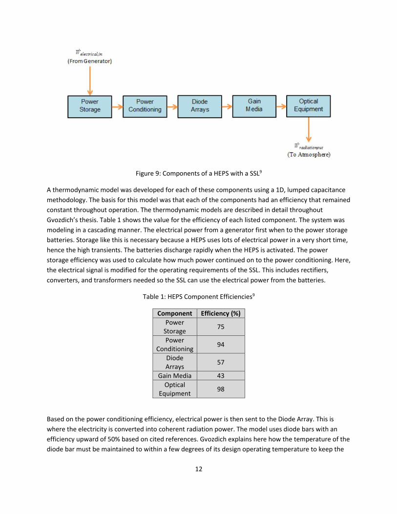
single heat load. As shown in Figure 9, Gvozdich created a detailed model of the HEPS utilizing a solid-

state laser (SSL) operating at room temperature containing Power Storage, Power Conditioning, Diode

Arrays, Gain Media, and Optical Equipment.

12

Figure 9: Components of a HEPS with a SSL9

A thermodynamic model was developed for each of these components using a 1D, lumped capacitance

methodology. The basis for this model was that each of the components had an efficiency that remained

constant throughout operation. The thermodynamic models are described in detail throughout

Gvozdich’s thesis. Table 1 shows the value for the efficiency of each listed component. The system was

modeling in a cascading manner. The electrical power from a generator first when to the power storage

batteries. Storage like this is necessary because a HEPS uses lots of electrical power in a very short time,

hence the high transients. The batteries discharge rapidly when the HEPS is activated. The power

storage efficiency was used to calculate how much power continued on to the power conditioning. Here,

the electrical signal is modified for the operating requirements of the SSL. This includes rectifiers,

converters, and transformers needed so the SSL can use the electrical power from the batteries.

Table 1: HEPS Component Efficiencies9

Component Efficiency (%)

Power Storage

75

Power Conditioning

94

Diode Arrays

57

Gain Media 43

Optical Equipment

98

Based on the power conditioning efficiency, electrical power is then sent to the Diode Array. This is

where the electricity is converted into coherent radiation power. The model uses diode bars with an

efficiency upward of 50% based on cited references. Gvozdich explains here how the temperature of the

diode bar must be maintained to within a few degrees of its design operating temperature to keep the

13

output power from the diodes within the wavelength absorption band of the gain media. This optical

power from the diodes is then absorbed by the gain media. Thermal management of the gain media is

important as well. After being absorbed by the gain media and losing yet more power to the

inefficiencies, the optical power radiation is put through an optical equipment model. This contains the

bean control, filters, mirrors, and structures to coalesce, reshape, and direct the radiation in the desired

manner. From here, the radiation beam of optical energy now travels downrange out of the HEPS.

Gvozdich goes on to explain the implementation of his HEPS-type model into the INVENT T2T Aircraft

Model for the purpose of performing thermal management analysis. The INVENT Program is an initiative

started by the Air Force to obtain a detailed and conceptual understanding of the future of thermal

management for air vehicles. For more background on the INVENT program, refer to papers written by

Bodie et al10, Walters et al11, and Wolff12. The work done by Gvozdich is similar to work done by

Donovan7 and Nuzum8 in how the focus is the on the power thermal interactions between a HEPS and a

T2T model.

Gvozdich takes modeling a HEPS further by modeling the individual components. However, these

component models still have a constant efficiency, regardless of the component temperature. He

acknowledges how component temperature plays a role in HEPS performance but does not quantify the

effect of changing temperature on efficiency. The research described in this literature review does not

contain any modeling/simulation of the dynamic efficiency phenomenon observed in HEPS components.

This shows the relevance of the proposed research in the Introduction section of this thesis, as it will

bridge the apparent gap in current HEPS modeling shown by this literature review. Modeling the

dynamic efficiencies of HEPS components is the next logical step in achieving better simulation data for

determining more effective designs of HEPS thermal management systems.

Exploratory Research and Study:

With this apparent gap in knowledge concerning the understanding of HEPS efficiency, this proposed

research is proven substantially relevant. An extensive amount of preliminary research is required to

comprehend the dynamically efficient nature of a HEPS. This beginning research focused on learning

more about laser beams, fiber lasers, methods to model them in terms of spectral power density and

developing a method to quantify the optical output from each component and follow it through each

cascading component. Research was also accomplished to understand the details into how temperature

affects the component efficiency.

Background on Fiber Lasers:

The process of producing a laser beam requires a source (laser diodes) to pump a gain medium and

optical equipment to focus the energy coming out of the gain medium. A fiber laser has been chosen for

use in this research due to its excellent performance characteristics in high power application. The name

fiber laser is in reference to using a kind of fiber optics for the gain medium, according to Tünnermann

et al13. This article states that fiber lasers have fantastic thermo-optical properties when compared to

14

most other types of lasers. This due to the large surface-to-volume ratio of the fiber. This large surface

area yields excellent heat disspiation along the length of the fiber. The fiber consists of a core

surrounded by cladding, which has a refractive index slightly lower than that of the core. The core

directs the light by complete internal reflection. The beam quality is so excpetional through a fiber that

it forms up as a near perfect Gaussian Beam. Hence, modeing the optical output using a Gaussian Curve

is valid for the fiber as well as the laser diode. Figure 10 below shows two diagrams of how a fiber laser

operates.

Figure 10: Simple Fiber Laser Diagram showing Core and Cladding13

As the pump light travels down the fiber, it is slowly absorbed over the entire length of the fiber and is

changed into high brightness, high power, and coherent laser radiation. The signal gain can be many

orders of magnitude higher in fibers versus SSL counterparts. This yields a fiber laser system with very

efficient operation and low pump threshold values, meaning it does not take much power from the

pump source before the gain medium activates. A fiber with Ytterbium-doped glass can see optical

efficiencies well above 80%13. This gives another reason as to why a fiber laser is a good choice for this

research. As fiber laser technology advances, the pulsed firing of these systems is becoming an area of

intense study. The term ultrafast is used to describe scenarios where the pulse of lasing is on the order

of ficoseconds in length. Figure 11 is provided below for a reference into the evolution of ultrafast fiber

amplifiers. Notice the large increase in fiber laser power. This shows great potential for increasingly

15

viable high power fiber lasers in the future, making the choice of fiber lasers for this research all the

more relevant for future work.

Figure 11: Power Evolution of Ultrafast Fiber Lasers13

Modeling the Laser Beam:

Lasers operate on the principle of stimulated emission. As stated earlier, a laser beam is

monochromatic, coherent, and highly collimated. It might seem like a challenging prospect to model a

laser beam and the energy contained within. However, Sun provides a place to begin with his excellent

book on the basics of laser diode beams14. He gives evidence to show that in his experience, the output

of a laser diode can be represented with negligible error using a Gaussian Curve. The model depends on

the center wavelength and the full width half maximum (FWHM) of the laser diode. Use of a Gaussian

Curve modeling methodology allows the spectral power density over a range of wavelength to be

shown. This is representative of the output wavelength of a given laser diode and the focus of the

output power around that wavelength. Figure 12 is an example of how the Gaussian Curve model would

be used to simulate laser diode output.

16

Figure 12: Diagram Showing Basics of Gaussian Curve Model for Laser Diode Output

λcenter LD (nominal center wavelength of laser diode) and λfwhm LD (laser diode FWHM) are parameters

taken directly from a laser diode. These parameters vary between diode types and sometimes even vary

between diodes of the same type due to manufacturing processes. The output is spectral power density,

normally in units of W/m. A Gaussian Curve can be modeled mathematically for the specific application

of laser diodes in equation 1 shown below.

𝑓(𝜆) = 𝐴𝑒−

(𝜆−𝜆𝑐𝑒𝑛𝑡𝑒𝑟 𝐿𝐷

)2

2𝑐2 |

𝑚

𝑛

(1)

A Gaussian curve is a continuous function over the entire domain. The wavelength is represented by λ.

The variables n and m are the bounds for the range of values for λ used to form the curve shown in

Figure 12. A is the peak of the curve, and c is the standard deviation of the curve based on the FWHM. If

all these values are known, the output of a laser diode can be reliably modeled using a Gaussian Curve.

The FWHM determines the concentration of optical power around the center wavelength. The laser

diode industry uses the FWHM value to specify and quantify the beam divergence. Beam divergence is

important concerning the optics aspect of study, but it goes to a level of detail that is beyond the scope

of this research. The concept of using a Gaussian Curve to simulate the power contained in a laser beam

is central to developing an accurate HEPS model.

Laser Diode Parameters:

Given this idea of the optical power output of a laser diode being centered on a specified wavelength, it

is important to understand the potential impact of temperature on the performance. Indeed, this

phenomenon of laser diode output wavelength shift due to temperature change does exist and has

been thoroughly studied in research by Kondow et al15, Welford et al16, and Adams et al17. Kondow’s

research is the most complete of these sources and explains how laser diodes are designed to output at

a certain wavelength. This design wavelength can vary for different applications. If the laser diode

changes temperature, this induces a wavelength shift in the optical output power. Kondow et al15

17

measured the temperature dependence of lasing wavelength of 1.2 to 1.3 μm for GaInNAs laser diodes

and found a value of 0.42 nm/°C15. This parameter represents the change in λcenter LD as the laser diode

temperature changes from its design reference temperature. Welford finds a value of 0.23 nm/°C in

Table 2 for a (GaAl)As laser diode16. This shows how different laser diodes will have a different shift

coefficient. More importantly, however, this work shows that the temperature change of a laser diode

effects its optical power output in terms of a shifting center wavelength. This will now be called the

wavelength temperature coefficient 𝜆𝑇 𝑐𝑜𝑒𝑓𝑓.

Since a laser diode’s output wavelength is based on temperature, equation 2 was created to represent

the actual center wavelength of a laser diode stack exposed to a temperature change. The current

temperature of the diode stack is compared to a reference temperature, and the equation yields the

actual center wavelength of the laser diode output compared to the nominal center wavelength at some

reference temperature.

𝜆𝑐𝑒𝑛𝑡𝑒𝑟 𝐿𝐷(𝑥) = 𝜆𝑐𝑒𝑛𝑡𝑒𝑟 𝐿𝐷 + ((𝑇𝐿𝐷(𝑥) − 𝑇𝑟𝑒𝑓 𝐿𝐷) ∗ 𝜆𝑇 𝑐𝑜𝑒𝑓𝑓) (2)

In this equation, x goes from 1 to 𝑁𝑈𝑀𝐿𝐷 𝑠𝑡𝑎𝑐𝑘𝑠. This creates a vector to store all the stack temperatures

and their corresponding current center wavelength. With a temperature change, the equaiton yields a

center wavelength different from the nominal center wavelength. In this way, the effect of temperature

change on a laser diode’s output can be quantified.

𝜆𝑇 𝑐𝑜𝑒𝑓𝑓 is not the only important laser diode parameter. To understand laser diode performance, several

parameters governing their operation must be understood. A list of these parameters and their

description are given in Table 2, with information taken from Kondow et al15, Hertsens18, and

OdicForce19.

Table 2: Important Laser Diode Characteristics

Parameter Name Description 𝐼𝑚𝑎𝑥 Max Current per Laser Diode (Amps) 𝐼𝑡ℎ Threshold Current (Amps)

𝑇𝑟𝑒𝑓 𝐿𝐷 Reference Temperature for Laser Diode Characteristics (°C) 𝑉𝑓𝑤𝑑 Laser Diode Forward Voltage Drop

𝜆𝑐𝑒𝑛𝑡𝑒𝑟 𝐿𝐷 Nominal Center Wavelength of Laser Diode Output at 𝑇𝑟𝑒𝑓 𝐿𝐷 (m)

𝜆𝑓𝑤ℎ𝑚 𝐿𝐷 Full Width Half Maximum of Laser Diode Output (m) 𝜆𝑇 𝑐𝑜𝑒𝑓𝑓 Wavelength Temperature Coefficient for Laser Diode (m/°C) 𝜂𝐿𝐷𝑠𝑙𝑜𝑝𝑒 Laser Diode Slope Efficiency (W/Amp)

The threshold current and laser diode slope efficiency require some more explanation here. Threshold

current is simply the current that must be provided to the laser diode before it starts lasing (producing

optical power) 18. Figure 13 shows this phenomenon in action.

18

Figure 13: Threshold Current vs. Optical Output Power of a Laser Diode19

Note how very little optical power is produced until the threshold current is reached. The laser diode

slope efficiency is the slope of the black line from the threshold current to the operating current (shown

as Iop in Figure 13) or the maximum current allowable for one laser diode18.

Laser Diode Packaging:

The power conversion efficiency of a laser diode is high, on the order of 50% to 60%20. Even with this

efficiency, a single laser diode alone cannot attain anywhere near the 100s of kWs required for a HEPS.

Hence, an array of many laser diodes must be used to achieve these high power levels. Several

individual laser diodes can be arranged in the form of bars4. These bars, or stacks, provide a means by

which to thermally manage several diodes at once (as the coolant can be used to cool the stack, in turn

cooling the diode) and a sort of thermal storage for the heat from the diode as well. The use of stacks

also allow several diodes to be operated at (or near) the same temperature, theoretically yielding beams

of the same center wavelength from each diode on the stack. This assumption of constant diode

temperature across a stack will be used in the HEPS model. Figure 14 gives a good visualization of using

stacks for a potential diode array design layout.

19

Figure 14: Laser Diode Array Packaging Diagram

The laser diodes receive electrical power to produce the beams. As per Figure 14, an array contains laser

diodes wired in both series and parallel. 𝑁𝑈𝑀𝐿𝐷 𝑠𝑡𝑎𝑐𝑘𝑠 is the number of diodes wired in series. It also

gives the number of stacks present in the array. 𝑁𝑈𝑀𝐿𝐷/𝑠𝑡𝑎𝑐𝑘 is the number of diodes in parallel. It is

representative of the number of diodes on each stack. These two values multiplied together will yield

the total number of laser diodes in the array. The array will be referenced from this point forward in the

following form: (𝑁𝑈𝑀𝐿𝐷/𝑠𝑡𝑎𝑐𝑘 x 𝑁𝑈𝑀𝐿𝐷 𝑠𝑡𝑎𝑐𝑘𝑠). This will allow the array size to be described easily.For

example, a (4 x 3) array has four laser diodes per stack and three stacks for a total of 12 laser diodes.

Each array of laser diodes is considered a module, and a certain number of these modules are used so

enough laser diodes exist between all the modules to yield the required design optical power output of

the HEPS. A schematic showing an example of how these modules could be laid out is shown in Figure

15.

20

Figure 15: Laser Diode Modules Diagram, Array Size (4 x 4)

The number of modules can be caluclated when the design optical power for the HEPS and the number

of diodes in series and parallel have been chosen. The equation for this is shown below in equation 3.

𝑁𝑢𝑚𝑀𝑜𝑑𝑢𝑙𝑒𝑠 =𝑃𝑜𝑤𝑒𝑟𝑜𝑝𝑡𝑖𝑐𝑎𝑙

𝑃𝑜𝑤𝑒𝑟𝑝𝑒𝑟 𝐿𝐷,𝑜𝑝𝑡∗𝑁𝑈𝑀𝐿𝐷 𝑠𝑡𝑎𝑐𝑘𝑠∗𝑁𝑈𝑀𝐿𝐷/𝑠𝑡𝑎𝑐𝑘 (3)

The total number of laser diodes requried to reach the design optical output power of the HEPS is

defined below in equation 4.

𝑁𝑢𝑚𝐷𝑖𝑜𝑑𝑒𝑠 = 𝑁𝑈𝑀𝐿𝐷 𝑠𝑡𝑎𝑐𝑘𝑠 ∗ 𝑁𝑈𝑀𝐿𝐷/𝑠𝑡𝑎𝑐𝑘 ∗ 𝑁𝑈𝑀𝑀𝑜𝑑𝑢𝑙𝑒𝑠 (4)

These parameters can vary by packaging design, but the number of diodes per each module was kept to

a perfect square (1, 4, 9, 16, 25…). This way, the number of diodes in series and parallel could be the

same if desired. If all diodes on one stack are assumed to be the same temperature, the stack can be

considered that temperature. The temperature of each stack can then be found using the heat

generated from the diodes on each stack and evaluating the energy equation using a 1D lumped

capacitance-type model9,21. This assumption of lumped capacitance is used later on when modeling the

HEPS in Simulink. In modeling the diode packaging this way, the thermal effects of having more diodes in

parrallel compared to more in series or a different number of modules altogether can be quantified.

21

The HEPS model does track the required electrical power needed for each laser diode array. Given a

certain amount of amperage and voltage being supplied to the diode array, the amperage seen by each

diode is the supplied amperage divided by the number of diodes in parallel. The voltage seen by each

diode is the supplied voltage divided by the number of diodes in series.

HEPS Efficiency Definitions:

Since a HEPS overall efficiency is dynamic, metrics must be created to quantify the efficiency while the

device is in operation. These allow a way to compare the electrical power into and out of the laser.

Equations 5 and 6 measure the optical efficiency.

𝜂𝑜𝑣𝑒𝑟𝑎𝑙𝑙 =𝑃𝑜𝑤𝑒𝑟𝑜𝑝𝑡𝑖𝑐𝑎𝑙 𝐴𝑆𝐸

𝑃𝑜𝑤𝑒𝑟𝑊𝑎𝑙𝑙 𝑃𝑙𝑢𝑔 (5)

𝜂𝑒𝑓𝑓𝑒𝑐𝑡𝑖𝑣𝑒 =𝑃𝑜𝑤𝑒𝑟𝑜𝑝𝑡𝑖𝑐𝑎𝑙 𝐴𝑆𝐸

𝑃𝑜𝑤𝑒𝑟 𝑂𝑢𝑡𝑜𝑝𝑡𝑖𝑐𝑎𝑙,𝑚𝑎𝑥 (6)

In equation 5, the overall efficiency is the amount of power out of the last HEPS component before the

laser beam is sent out (𝑃𝑜𝑤𝑒𝑟𝑜𝑝𝑡𝑖𝑐𝑎𝑙 𝐴𝑆𝐸) over the electrical power being provided to the HEPS. This is

important for obtaining an idea of the amount of optical power out of the HEPS versus the electrical

power supplied to the HEPS.

In equation 6, the effective efficiency is 𝑃𝑜𝑤𝑒𝑟𝑜𝑝𝑡𝑖𝑐𝑎𝑙 𝐴𝑆𝐸 over the maximum possible optical power out.

This parameter tells how close the actual HEPS efficiency is to its maximum value. This maximum value

is a theoretical value calculated from conditions at which the HEPS is operating at its maximum

efficiency. At this condition, all internal components are operating their peak efficiency. When this value

is at 100%, the HEPS is at its optimum operating point. Remember, 𝑃𝑜𝑤𝑒𝑟𝑜𝑝𝑡𝑖𝑐𝑎𝑙 𝐴𝑆𝐸 is going to be

constantly changing as the temperature of internal components change. This is why temperature control

of internal components is such a concern. In simulation, the goal is to optimize parameters so that

throughout operation, the effective efficiency stays as close as possible to 100% which gives the best

HEPS performance.

Models Created in MATLAB/Simulink:

The models created are based in the MATLAB/Simulink environment. As such, the analysis will utilize 1D

lumped capacitance methods. The idea of modeling in the Simulink environment lends itself well to

building the actual models because everything can be created in terms of components. These

components are “block diagrams” in the Simulink space. When the components are created, they are

independent in that they can be put into any other model and used given they are initialized correctly

with the proper files. This is a very organized way of modeling because the subsystems can be put inside

the main component block and kept in a neat and orderly fashion, allowing the governing equations to

be inserted and adjusted as necessary. Certain parts of a system could easily be added into or taken out

of the model with this approach. As with all models, the ones presented in this section are based on

assumptions. This means taking the necessary governing equations and simplifying those using

22

experimental results, engineering knowledge, and at some points making an educated estimate or guess

to provide closure in order to make the governing equations solvable. Hence, it is of paramount

importance to understand exactly how the model was created, as understanding the assumptions within

are critical in knowing to what extent the model results are accurate for use in simulation and

optimization of a real-life system. If the model assumptions and limitations are not properly

documented, it is impossible to know for certain the model’s potential usefulness and accuracy.

Therefore, the HEPS model and its palletized system for thermal management are fully described and

documented.

Temperature Sensitive HEPS Model:

The HEPS model was created to simulate the thermal and efficiency characteristics of a fiber laser while

in operation. Specifically, the temperatures of the internal components and their respective efficiencies

are the model’s focus. It was made to be a block in the Simulink environment so it could be moved and

used as a subsystem in any larger thermal management model. The model contains 3 main internal

HEPS components: Laser diodes, gain medium, and combiner. The combiner has 3 sub components:

Beam director, mirrors, and aperture sharing element. The optical power output of the laser diodes is

calculated, and the subsequent absorption of this energy by the gain medium is calculated as well. The

laser diode temperatures are important for this model’s operation. The gain medium temperature,

while every bit as important, is not taken into account in this model. Even though gain medium

absorption is very temperature dependent, it is simply beyond the scope of this research in terms of

both complexity and available time. The gain medium efficiency is held constant. The same goes for the

combiner. This component is based on very complicated optics, and its efficiency will also be held

constant for this model as that work is also beyond the scope of this research. Hence, the only

component performance based on temperature is the laser diodes. It will be seen how complicated it is

to model just the temperature dependent laser diodes alone. The model needs to track not only the

temperature change of the internal components due to heat generation, but also the temperature of

the cooling fluid as it flows through these components. The temperature change of internal components

is calculated based on the particular component’s heat plate temperature. The component temperature

is no longer confined to a certain temperature range, as was the case in work done by Gvozdich9 and

Nuzum3. Instead, the now dynamic efficiency of the HEPS can be monitored and the effect of this

temperature fluctuation on efficiency can be observed.

All the equations shown in this section are solved in the HEPS Simulink model. This system of equations

was created specifically for this model from knowledge learned in the exploratory study and research. In

order to solve the equations that determine HEPS performance, some parameters must first be defined.

These are specified in the beginning of the problem, and the model uses these parameters to

subsequently solve for any other variables needed in the equation. It is pertinent to list them out here in

Table 3, noting they are also listed in the nomenclature section.

23

Table 3: HEPS Parameters Initially Defined

Parameter – Definition

𝑇𝑟𝑒𝑓 𝐿𝐷 – Reference Temperature for Laser Diode Characteristics (°C)

𝑇𝑖𝑛 𝐿𝐷 – Temperature of Coolant Fluid into Laser Diode (°C)

𝑇𝑜𝑢𝑡 𝐿𝐷 – Temperature of Coolant Fluid out of Laser Diode (°C)

𝜆𝑐𝑒𝑛𝑡𝑒𝑟 𝐿𝐷 – Nominal Center Wavelength of Laser Diode Output at 𝑇𝑟𝑒𝑓 𝐿𝐷 (m)

𝜆𝑓𝑤ℎ𝑚 𝐿𝐷 – Full Width Half Maximum of Laser Diode Output (m)

𝜆𝑇 𝑐𝑜𝑒𝑓𝑓 – Wavelength Temperature Coefficient for Laser Diode (m/°C)

𝐼𝑡ℎ - Threshold Current (Amps)

𝐼𝑚𝑎𝑥 – Max Current per Laser Diode (Amps)

𝑁𝑈𝑀𝐿𝐷/𝑠𝑡𝑎𝑐𝑘 – Number of Laser Diodes per Stack (diodes in parallel)

𝑉𝑓𝑤𝑑 – Laser Diode Forward Voltage Drop per Stack

𝜂𝐿𝐷𝑠𝑙𝑜𝑝𝑒 – Laser Diode Slope Efficiency (W/Amp)

𝑅𝑜𝑙𝑙𝑜𝑣𝑒𝑟𝑐𝑜𝑒𝑓𝑓 – Coefficient for Laser Diode Rollover Power

𝜂max 𝐺𝑀 – Peak Efficiency of Gain Medium at Center Wavelength

𝜆𝑐𝑒𝑛𝑡𝑒𝑟 𝐺𝑀 – Center Wavelength of Gain Medium Absorption Spectrum (m)

𝜆𝑓𝑤ℎ𝑚 𝐺𝑀 – Full Width Half Maximum of Gain Medium Absorption Peak (m)

𝜂𝐵𝐷 – Beam Director Thermal Efficiency

𝜂𝑀𝑅 – Optical Training Mirror Lumped Reflectivity

𝜂𝐴𝑆𝐸 – Aperture Sharing Element Thermal Efficiency

𝑃𝑜𝑤𝑒𝑟𝑜𝑝𝑡𝑖𝑐𝑎𝑙 – HEPS Design Optical Power from Laser Diodes (W)

𝑃𝑜𝑤𝑒𝑟𝑤𝑎𝑙𝑙 𝑝𝑙𝑢𝑔 – HEPS Wall Plug Power (W)

From these defined input parameters, all other needed values can be calculated. The equations that

follow will define the process by which the model does calculations to find the HEPS efficiency. There

are more input variables that must be determined before the calculations start, and the parameters

from Table 3 are used to find these other input variables. Equations 7 through 14 are presented in such

an order that they only use variables already calculated or known. This allows the calculations to

proceed in a logical, easily followed manner. Once values are known, they can then be used to do

subsequent calculations.

𝑃𝑜𝑤𝑒𝑟𝑝𝑒𝑟 𝐿𝐷,𝑜𝑝𝑡 – Nominal Optical Power per Laser Diode at center wavelength λ (W)

𝑃𝑜𝑤𝑒𝑟𝐿𝐷,𝑜𝑝𝑡 = 𝐼𝑚𝑎𝑥 ∗ 𝜂𝐿𝐷𝑠𝑙𝑜𝑝𝑒 (7)

𝑁𝑈𝑀𝐿𝐷 𝑠𝑡𝑎𝑐𝑘𝑠 – Number of Laser Diode Stacks (diodes in series)

𝑁𝑈𝑀𝐿𝐷 𝑠𝑡𝑎𝑐𝑘𝑠 =𝑃𝑜𝑤𝑒𝑟𝑜𝑝𝑡𝑖𝑐𝑎𝑙

(𝑁𝑈𝑀𝐿𝐷/𝑠𝑡𝑎𝑐𝑘∗𝑃𝑜𝑤𝑒𝑟𝑝𝑒𝑟 𝐿𝐷,𝑜𝑝𝑡) (8)

24

𝐼𝐻𝐸𝑃𝑆 – Current to HEPS (Amps)

𝐼𝐻𝐸𝑃𝑆 = 𝐼𝑚𝑎𝑥 ∗ 𝑁𝑈𝑀𝐿𝐷/𝑠𝑡𝑎𝑐𝑘 (9)

𝑉𝐻𝐸𝑃𝑆 – Voltage to HEPS (Volts)

𝑉𝐻𝐸𝑃𝑆 =𝑃𝑜𝑤𝑒𝑟𝑤𝑎𝑙𝑙 𝑝𝑙𝑢𝑔

𝐼𝐻𝐸𝑃𝑆 (10)

𝑉𝑝𝑒𝑟 𝐿𝐷 – Voltage per Laser Diode (Volts)

𝑉𝑝𝑒𝑟 𝐿𝐷 =𝑉𝐻𝐸𝑃𝑆

𝑁𝑈𝑀𝐿𝐷 𝑠𝑡𝑎𝑐𝑘𝑠 (11)

𝑃𝑜𝑤𝑒𝑟𝑟𝑜𝑙𝑙𝑜𝑣𝑒𝑟 – Rollover Power in terms of Optical Output Power (W)

𝑃𝑜𝑤𝑒𝑟𝑟𝑜𝑙𝑙𝑜𝑣𝑒𝑟 = 𝑃𝑜𝑤𝑒𝑟𝑝𝑒𝑟 𝐿𝐷,𝑜𝑝𝑡 ∗ 𝑅𝑜𝑙𝑙𝑜𝑣𝑒𝑟𝑐𝑜𝑒𝑓𝑓 (12)

𝑃𝑜𝑤𝑒𝑟𝑝𝑒𝑟 𝐿𝐷,𝑒𝑙𝑒𝑐 – Electrical Power per Laser Diode (W)

𝑃𝑜𝑤𝑒𝑟𝑝𝑒𝑟 𝐿𝐷,𝐸𝑙𝑒𝑐 = 𝑉𝑝𝑒𝑟 𝐿𝐷 ∗ 𝐼𝑚𝑎𝑥 (13)

𝜂𝐿𝐷,𝑚𝑎𝑥 – Max Laser Diode Efficiency

𝜂𝐿𝐷,𝑚𝑎𝑥 =𝑃𝑜𝑤𝑒𝑟𝑝𝑒𝑟 𝐿𝐷,𝑜𝑝𝑡

𝑃𝑜𝑤𝑒𝑟𝑝𝑒𝑟 𝐿𝐷,𝐸𝑙𝑒𝑐 (14)

The variable 𝑇𝐿𝐷(𝑥) from equation 2 is the laser diode stack temperatures.

The variable x goes from 1 to 𝑁𝑈𝑀𝐿𝐷 𝑠𝑡𝑎𝑐𝑘𝑠 to represent all the stack temperatures. The values for this

variable come from the thermal bookkeeping side of the model, not within the HEPS model itself. This

thermal bookkeeping is described in the HEPS Cooling Loop: section.

With all these variables defined and preliminary calculations solved, the model can now use these values

to do the actual optical power production calculations. There is no power conditioning model here, so

rectifiers, converters, and the like are not modeled. It is assumed the HEPS can get electrical power at

the proper voltage, amperage, and phase it requires instantaneously. This removes the need to model

the complicated electronics that are outside the scope of this research.

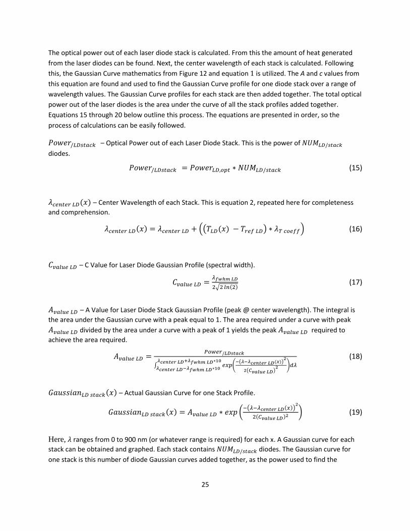
25

The optical power out of each laser diode stack is calculated. From this the amount of heat generated

from the laser diodes can be found. Next, the center wavelength of each stack is calculated. Following

this, the Gaussian Curve mathematics from Figure 12 and equation 1 is utilized. The A and c values from

this equation are found and used to find the Gaussian Curve profile for one diode stack over a range of

wavelength values. The Gaussian Curve profiles for each stack are then added together. The total optical

power out of the laser diodes is the area under the curve of all the stack profiles added together.

Equations 15 through 20 below outline this process. The equations are presented in order, so the

process of calculations can be easily followed.

𝑃𝑜𝑤𝑒𝑟/𝐿𝐷𝑠𝑡𝑎𝑐𝑘 – Optical Power out of each Laser Diode Stack. This is the power of 𝑁𝑈𝑀𝐿𝐷/𝑠𝑡𝑎𝑐𝑘

diodes.

𝑃𝑜𝑤𝑒𝑟/𝐿𝐷𝑠𝑡𝑎𝑐𝑘 = 𝑃𝑜𝑤𝑒𝑟𝐿𝐷,𝑜𝑝𝑡 ∗ 𝑁𝑈𝑀𝐿𝐷/𝑠𝑡𝑎𝑐𝑘 (15)

𝜆𝑐𝑒𝑛𝑡𝑒𝑟 𝐿𝐷(𝑥) – Center Wavelength of each Stack. This is equation 2, repeated here for completeness

and comprehension.

𝜆𝑐𝑒𝑛𝑡𝑒𝑟 𝐿𝐷(𝑥) = 𝜆𝑐𝑒𝑛𝑡𝑒𝑟 𝐿𝐷 + ((𝑇𝐿𝐷(𝑥) − 𝑇𝑟𝑒𝑓 𝐿𝐷) ∗ 𝜆𝑇 𝑐𝑜𝑒𝑓𝑓) (16)

𝐶𝑣𝑎𝑙𝑢𝑒 𝐿𝐷 – C Value for Laser Diode Gaussian Profile (spectral width).

𝐶𝑣𝑎𝑙𝑢𝑒 𝐿𝐷 =𝜆𝑓𝑤ℎ𝑚 𝐿𝐷

2√2 𝑙𝑛(2) (17)

𝐴𝑣𝑎𝑙𝑢𝑒 𝐿𝐷 – A Value for Laser Diode Stack Gaussian Profile (peak @ center wavelength). The integral is

the area under the Gaussian curve with a peak equal to 1. The area required under a curve with peak

𝐴𝑣𝑎𝑙𝑢𝑒 𝐿𝐷 divided by the area under a curve with a peak of 1 yields the peak 𝐴𝑣𝑎𝑙𝑢𝑒 𝐿𝐷 required to

achieve the area required.

𝐴𝑣𝑎𝑙𝑢𝑒 𝐿𝐷 =𝑃𝑜𝑤𝑒𝑟/𝐿𝐷𝑠𝑡𝑎𝑐𝑘

∫ 𝑒𝑥𝑝 (−(𝜆−𝜆𝑐𝑒𝑛𝑡𝑒𝑟 𝐿𝐷(𝑥))

2

2(𝐶𝑣𝑎𝑙𝑢𝑒 𝐿𝐷)2 )𝑑𝜆

𝜆𝑐𝑒𝑛𝑡𝑒𝑟 𝐿𝐷+𝜆𝑓𝑤ℎ𝑚 𝐿𝐷∗10

𝜆𝑐𝑒𝑛𝑡𝑒𝑟 𝐿𝐷−𝜆𝑓𝑤ℎ𝑚 𝐿𝐷∗10

(18)

𝐺𝑎𝑢𝑠𝑠𝑖𝑎𝑛𝐿𝐷 𝑠𝑡𝑎𝑐𝑘(𝑥) – Actual Gaussian Curve for one Stack Profile.

𝐺𝑎𝑢𝑠𝑠𝑖𝑎𝑛𝐿𝐷 𝑠𝑡𝑎𝑐𝑘(𝑥) = 𝐴𝑣𝑎𝑙𝑢𝑒 𝐿𝐷 ∗ 𝑒𝑥𝑝 (−(𝜆−𝜆𝑐𝑒𝑛𝑡𝑒𝑟 𝐿𝐷(𝑥))

2

2(𝐶𝑣𝑎𝑙𝑢𝑒 𝐿𝐷)2 ) (19)

Here, 𝜆 ranges from 0 to 900 nm (or whatever range is required) for each x. A Gaussian curve for each

stack can be obtained and graphed. Each stack contains 𝑁𝑈𝑀𝐿𝐷/𝑠𝑡𝑎𝑐𝑘 diodes. The Gaussian curve for

one stack is this number of diode Gaussian curves added together, as the power used to find the

26

Gaussian curve peak (𝐴𝑣𝑎𝑙𝑢𝑒 𝐿𝐷) for each stack is the combined power of all didoes on that one stack,

again assuming the stack/junction is uniform in temperature.

𝐺𝑎𝑢𝑠𝑠𝑖𝑎𝑛𝑎𝑙𝑙 𝑠𝑡𝑎𝑐𝑘𝑠 – Gaussian Curve for all Stack Profiles added together to form one curve. It is the

output curves of all laser diodes added together to make a single curve.

𝐺𝑎𝑢𝑠𝑠𝑖𝑎𝑛𝑎𝑙𝑙 𝑠𝑡𝑎𝑐𝑘𝑠 = ∑ 𝐺𝑎𝑢𝑠𝑠𝑖𝑎𝑛𝐿𝐷 𝑠𝑡𝑎𝑐𝑘(𝑥)𝑁𝑈𝑀𝐿𝐷 𝑠𝑡𝑎𝑐𝑘𝑠𝑥=1 (20)

𝑃𝑜𝑤𝑒𝑟𝑜𝑝𝑡𝑖𝑐𝑎𝑙 𝐿𝐷 – Total optical power out of all laser diodes, area under 𝐺𝑎𝑢𝑠𝑠𝑖𝑎𝑛𝑎𝑙𝑙 𝑠𝑡𝑎𝑐𝑘𝑠

The main value of concern from the laser diode calculations is 𝑃𝑜𝑤𝑒𝑟𝑜𝑝𝑡𝑖𝑐𝑎𝑙 𝐿𝐷. This is the value that

cascades into the next set of computations for the gain medium. All electrical power not converted to

optical power by the laser diodes is considered lost as heat. The optical power out of the laser diodes is

the input optical power to the gain medium. From the laser diodes, the calculations then move onto the

gain medium. The gain medium has its own specific center wavelength and wavelength FWHM. These

correspond to the laser diode output allowing the gain medium to absorb this optical power. When the

laser diode output shifts due to temperature change, this in turn has an effect on gain medium

absorption. Equations 21 through 23 below show and explain this process. They are again laid out in a

logical order so the process of calculations can be easily followed and understood.

𝐶𝑣𝑎𝑙𝑢𝑒 𝐺𝑚 – C value for Gain Medium Gaussian Profile

𝐶𝑣𝑎𝑙𝑢𝑒 𝐺𝑀 =𝜆𝑓𝑤ℎ𝑚 𝐺𝑀

2√2 ln(2) (21)

𝐴𝑏𝑠𝑜𝑟𝑝𝑡𝑖𝑜𝑛 𝐶𝑢𝑟𝑣𝑒𝐺𝑀 – Gain Medium Efficiency Absorption Profile (Gaussian Curve)

𝐴𝑏𝑠𝑜𝑟𝑝𝑡𝑖𝑜𝑛 𝐶𝑢𝑟𝑣𝑒𝐺𝑀 = 𝜂max 𝐺𝑀 ∗ 𝑒𝑥𝑝 (−(𝜆−𝜆𝑐𝑒𝑛𝑡𝑒𝑟 𝐺𝑀)2

2(𝐶𝑣𝑎𝑙𝑢𝑒 𝐺𝑀)2 ) (22)

𝜆 goes from 0 to 900 nm or whatever range is required. The A value is 𝜂max 𝐺𝑀 because the gain medium

efficiency is to be set. The next step creates a gain medium power absorption curve of the same

magnitude as the single Gaussian curve of the output of all laser diodes added together, only now the

gain medium efficiency can be set using the value 𝜂max 𝐺𝑀.

𝐴𝑏𝑠𝑜𝑟𝑝𝑡𝑖𝑜𝑛 𝑃𝑜𝑤𝑒𝑟𝐺𝑀 – Multiply input laser diode power across all wavelengths by the Gain Medium

Absorption Curve, this yields the actual gain medium absorption power curve that is close to the same

magnitude as the laser diode 𝐺𝑎𝑢𝑠𝑠𝑖𝑎𝑛𝑎𝑙𝑙 𝑠𝑡𝑎𝑐𝑘𝑠 curve.

𝐴𝑏𝑠𝑜𝑟𝑝𝑡𝑖𝑜𝑛 𝑃𝑜𝑤𝑒𝑟𝐺𝑀 = 𝐺𝑎𝑢𝑠𝑠𝑖𝑎𝑛𝑎𝑙𝑙 𝑠𝑡𝑎𝑐𝑘𝑠 ∗ 𝐴𝑏𝑠𝑜𝑟𝑝𝑡𝑖𝑜𝑛 𝐶𝑢𝑟𝑣𝑒𝐺𝑀 (23)

27

𝑃𝑜𝑤𝑒𝑟𝑜𝑝𝑡𝑖𝑐𝑎𝑙 𝐺𝑀 – Total area under the curve 𝐴𝑏𝑠𝑜𝑟𝑝𝑡𝑖𝑜𝑛 𝑃𝑜𝑤𝑒𝑟𝐺𝑀. This is the amount of optical

power out of the Gain Medium.

Any optical power that is not transferred to the gain medium is considered lost as heat. Notice how the

temperature of the gain medium is not taken into account. The optical power out of the gain medium

then cascades onward into the combiner. The combiner consists of three subcomponents, and each one

of these subcomponents has a set efficiency. The beam director, mirrors, and particularly the aperture

sharing element in fiber lasers are the controls that help guide the output of all the gain medium fibers

and help to coalesce all the individual laser beams into a single coherent, very high-power beam that is

then directed out of the HEPS. A paper by Begley et al22 describes combining the beams from a 10-diode

laser array and then the beams of 5 arrays (50 diodes) using a type of aperture sharing element. This

device has an efficiency that is very difficult to quantify, so it simply kept at a constant value. The

equations for calculating the optical power out of the combiner components are shown below by

equations 24 through 26.

For the beam director,

𝑃𝑜𝑤𝑒𝑟𝑜𝑝𝑡𝑖𝑐𝑎𝑙 𝐵𝐷 = 𝑃𝑜𝑤𝑒𝑟𝑜𝑝𝑡𝑖𝑐𝑎𝑙 𝐺𝑀 ∗ 𝜂𝐵𝐷 (24)

For the mirrors,

𝑃𝑜𝑤𝑒𝑟𝑜𝑝𝑡𝑖𝑐𝑎𝑙 𝑀𝑅 = 𝑃𝑜𝑤𝑒𝑟𝑜𝑝𝑡𝑖𝑐𝑎𝑙 𝐵𝐷 ∗ 𝜂𝑀𝑅 (25)

For the aperture sharing element,

𝑃𝑜𝑤𝑒𝑟𝑜𝑝𝑡𝑖𝑐𝑎𝑙 𝐴𝑆𝐸 = 𝑃𝑜𝑤𝑒𝑟𝑜𝑝𝑡𝑖𝑐𝑎𝑙 𝑀𝑅 ∗ 𝜂𝐴𝑆𝐸 (26)

This is the entire process of modeling the optical power out of the HEPS. Equations 15 through 26 were

built into Simulink for model simulation. The model was created with the ability to be easily

changed/improved later on. All the input variables are initialized through an Excel spreadsheet. In this

way, input parameters can be easily changed to run different studies. Changing the input parameters of

the HEPS model changes its operating characteristics. From these equations, a changing laser diode

stack temperature does not yield a significant decrease in laser diode optical output power. It instead

changes the center wavelength on which the diode it outputting. The optical power loss occurs in the

gain medium when diode output center wavelength no longer lines up with the gain medium absorption

center wavelength. A more in-depth explanation and graphical representation of this phenomenon is

discussed in the Model Testing Section.

HEPS Cooling Loop:

A HEPS produces large heat loads that must be dissipated. A cooling loop utilizing a 60% ethylene-glycol

water solution was modeled as an intermediate fluid between the HEPS operating at room temperature

and the LNG palletized TMS. The model was created in Simulink using components created in previous

28

research at Wright State University3,23. It includes storage tanks for the ethylene-glycol solution, pumps

to move this intermediate fluid, a heat exchanger for heat transfer between the ethylene-glycol solution

and cold natural gas, and heat plates for heat transfer between the HEPS components and the ethylene-

glycol solution. As these components were already created, they simply had to be integrated together in

a Simulink model. Figure 16 below shows a diagram for the layout of this model.

Figure 16: HEPS Cooling Loop Model Diagram

This cooling loop contains two storage tanks: One cold reservoir and one hot reservoir. Ethylene-glycol

solution from the cold reservoir is pumped through the Diodes, Fibers, and Combiner heat plate in

series. The fluid rises in temperature as it absorbs the heat generated by these three components in

series. The fluid then dumps into the hot reservoir. From here, the ethylene-glycol solution is pumped

through the heat exchanger and cooled by the cold natural gas flow from the palletized TMS (link to

palletized TMS section here). The flow rates from each pump are dependent on the activation state of

the HEPS and component temperature. A controller is used to determine the flow rate of each pump at

any given time based on these conditions. When the HEPS is activated, the cold reservoir pump is turned

on in attempt to keep the temperatures in check. The hot reservoir pump attempts to keep a specific

mass of coolant in the cold reservoir. For this model, everything is initially at room temperature.

The heat exchanger operates using a 1D lumped capacitance model. It contains the energy equations for

the heat transfer taking place between two fluids at different temperatures. It does not contain the

capability of doing two-phase calculations, as this model does not require this capability. The

temperature range seen by the ethylene-glycol solution in this model means it stays a liquid, and the

natural gas, while very cold, it still a gas. It is a multi-fluid heat exchanger with several different fluid

properties built in. The hot side fluid is the ethylene-glycol solution and the cold side fluid is Methane.

Methane is chosen to represent the liquefied natural gas because natural gas is composed of a very high

29

percentage of Methane. The heat exchanger material is Aluminum. The heat exchanger model comes

from Roberts et al23. A diagram of how the heat transfer takes place within the heat exchanger is shown

in Figure 17.

Figure 17: Heat Exchanger With Energy Flow in and out of Each Discrete Volume23

The cold fluid leaves at a higher temperature than which it entered, and the hot fluid leaves at a lower

temperature than which it entered. The model simulates a counter-flow plate fin heat exchanger. A

diagram of this is shown in Figure 18.

30

Figure 18: Plate Fin Configuration HX Geometry (fins serrated to promote turbulence)23

In the figure above, t is the plate thickness in between the hot and cold sides of the heat exchanger. The

fin height is represented by h and fin thickness by tf. The distance from the top of channel to the bottom

is b. The working fluid for the hot and cold sides flow through these channels is separated by the heat

exchanger plate material (Figure 17). Making the h in Figure 18 considerably small allows this heat

exchanger model to simulate the performance of a micro-channel heat exchanger. The heat exchanger

models use the Gnielinski Correlations to model flow through an offset strip fin (OSF) compact heat

exchanger.

The heat plates are one – sided heat exchangers. The hot side calculations of the heat exchanger are

taken out and replaced with an input for a heat load. For this case, Figure 17 would only have the cold

side with a heat load on the hot side of the heat exchanger material. This heat load is transferred to the

cold side fluid (ethylene-glycol solution) by solving the energy equations for heat transfer. The model

uses 𝑁𝑈𝑀𝑀𝑜𝑑𝑢𝑙𝑒𝑠 heat plates for the laser diodes and two more heat plates for the gain medium and

combiner components. The heat plates for the gain medium and combiner are identical to Butt25. Figure

19 shows how the diode stacks and corresponding heat plate surface integrate together in the model.

The cooling fluid flows on the opposite side of the heat plate.

Figure 19: Heat Plate Surface and Diode Stack Representation

The heat generated by the laser diode stacks is taken away by cooling fluid flowing on the opposite side

of the heat plate. The heat plate discrete volumes have a thickness of t from Figure 18. As stated earlier,

the thermal bookkeeping of the HEPS model is done by this cooling loop. The 1D lumped capacitance

assumption allows the heat plate calculations to be accomplished by discrete volumes. The laser diode

heat plate surface is broken up into 𝑁𝑈𝑀𝐿𝐷 𝑠𝑡𝑎𝑐𝑘𝑠 discrete volumes, one discrete volume represents one

laser diode stack. The heat plate calculations produce a temperature for each discrete volume. This is

the temperature of the heat plate surface section for each discrete volume. The laser diode stacks are

considered to be mounted directly on top of each heat plate section, as shown in Figure 19. The

31

assumption is made that the laser diode stack temperatures are equal to the temperature of the heat

plate section at each discrete volume. The temperature vector of each laser diode stack 𝑇𝐿𝐷(𝑥) is then

sent to the HEPS model where it is used in the calculations explained in the Temperature Sensitive HEPS

Model Section. This is the method for modeling the laser diode stack temperatures as a 1D lumped

capacitance model. The heat plate blocks in the Simulink model are shown below in Figure 20.

Figure 20: Simulink Block Diagram of Heat Plates for Three Major HEPS Components

Notice the similarity to the diagram of Figure 16. The three HEPS components are cooled by flow in

series. The laser diodes are cooled first followed by the gain medim and combiner. The laser diode heat

sent to the Laser Diode Heat Plate is the amount of heat produced by (𝑁𝑈𝑀𝐿𝐷/𝑠𝑡𝑎𝑐𝑘 x 𝑁𝑈𝑀𝐿𝐷 𝑠𝑡𝑎𝑐𝑘𝑠)

diodes. The heat sent to Gain Medium and Combiner heat plates is the total heat from each component.

There are as many laser diode heat plates as there are laser diode array modules. However, there is only

one laser diode heat plate in the model to speed up calculations. This works because each module

contains the same number of diodes and the amount of heat from each module will be the same.

Hence, the cooling flow in must be divided by 𝑁𝑈𝑀𝑀𝑜𝑑𝑢𝑙𝑒𝑠 to send cooling flow to each module. The

temperature of the cooling flow out of each module should be the same, and then the cooling flow is

multiplied by 𝑁𝑈𝑀𝑀𝑜𝑑𝑢𝑙𝑒𝑠 to set the cooling flow out to its actual value. This actual mass flow rate is

then sent on to the gain medium and combiner heat plates. This method simulates many modules at

one time without actually having to do the heat transfer and temperature calculations for every heat

plate and module.

Model Testing:

The following tests on the HEPS model were done using a test stand to see how the temperature shift

occurs and how it effects the power absorbed by the gain medium. The HEPS model wasn’t connected

to any other thermal management components for the tests. In this way, it could be determined if the

equations in the HEPS model were implemented correctly. Initial parameters were set for the model as

shown below in Table 4. These values are based on a mixture of sources mentioned previously and

estimated guesses, as the power-thermal trends are the focal point of this research.

32

Table 4: HEPS Model Initial Testing Parameter Values

Parameter – Definition Value

𝑇𝑟𝑒𝑓 𝐿𝐷 – Reference Temperature for Laser Diode Characteristics (°C) 12

𝜆𝑐𝑒𝑛𝑡𝑒𝑟 𝐿𝐷 – Nominal Center Wavelength of Laser Diode Output at 𝑇𝑟𝑒𝑓 𝐿𝐷 (m) 8.08e-07

𝜆𝑓𝑤ℎ𝑚 𝐿𝐷 – Full Width Half Maximum of Laser Diode Output (m) 5e-09

𝜆𝑇 𝑐𝑜𝑒𝑓𝑓 – Wavelength Temperature Coefficient for Laser Diode (m/°C) 2.7e-10

𝐼𝑡ℎ - Threshold Current (Amps) 20

𝐼𝑚𝑎𝑥 – Max Current per Laser Diode (Amps) 150

𝑁𝑈𝑀𝐿𝐷/𝑠𝑡𝑎𝑐𝑘 – Number of Laser Diodes per Stack (diodes in parallel) 10

𝑁𝑈𝑀𝐿𝐷 𝑠𝑡𝑎𝑐𝑘𝑠 – Number of Laser Diode Stacks (diodes in series) 100

𝑁𝑈𝑀𝑀𝑜𝑑𝑢𝑙𝑒𝑠 – Number of Modules 1

𝑉𝑓𝑤𝑑 – Laser Diode Forward Voltage Drop per Stack 1.9

𝜂𝐿𝐷𝑠𝑙𝑜𝑝𝑒 – Laser Diode Slope Efficiency (W/Amp) 1

𝑅𝑜𝑙𝑙𝑜𝑣𝑒𝑟𝑐𝑜𝑒𝑓𝑓 – Coefficient for Laser Diode Rollover Power 1.2

𝜂max 𝐺𝑀 – Peak Efficiency of Gain Medium at Center Wavelength 0.80

𝜆𝑐𝑒𝑛𝑡𝑒𝑟 𝐺𝑀 – Center Wavelength of Gain Medium Absorption Spectrum (m) 8.08e-07

𝜆𝑓𝑤ℎ𝑚 𝐺𝑀 – Full Width Half Maximum of Gain Medium Absorption Peak (m) 2e-08

𝜂𝐵𝐷 – Beam Director Thermal Efficiency 0.95

𝜂𝑀𝑅 – Optical Training Mirror Lumped Reflectivity 0.92

𝜂𝐴𝑆𝐸 – Aperture Sharing Element Thermal Efficiency 0.97

𝑃𝑜𝑤𝑒𝑟𝑜𝑝𝑡𝑖𝑐𝑎𝑙 – HEPS Design Optical Power from Laser Diodes (W) 150000

𝑃𝑜𝑤𝑒𝑟𝑤𝑎𝑙𝑙 𝑝𝑙𝑢𝑔 – HEPS Wall Plug Power (W) 306000

With these values being held constant, the operating temperature of the laser diode stacks could be

changed. The amount of optical power into the gain medium from the laser diodes for these tests is

constant at 148.4 kW. Since the thermal bookkeeping was not used in these tests, the temperature of

the laser diode stacks had to be manually set. For the 1st test shown in Figure 21, the laser diode stack

temperatures are all set to 12°C, meaning no deviation of stack temperature from the reference

temperature.

33

Figure 21: Laser Diode and Gain Medium Output (Diodes at Reference Temperature, 12°C)

The LD curve is the output curve of all the individual laser diode outputs added together. The area under

it represents the total power out of the laser diodes. The area under the GM Absorption curve is the

total power absorbed by the gain medium. The area in between these two curves represents the heat

generated within the gain medium. With no change in diode stack temperature, the peaks of both

curves are centered at 808 nm. With the given parameters, this case achieves the highest level of gain

medium absorption for the tests at 115.2 kW (~78% efficient). This makes sense as the laser diode stack

temperatures have not shifted as all making for ideal operation of the largest possible efficiency. For the

2nd test is shown in Figure 22, the diode stack temperatures are increasing linearly from 12°C to 22°C.

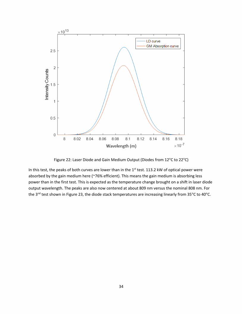
34

Figure 22: Laser Diode and Gain Medium Output (Diodes from 12°C to 22°C)

In this test, the peaks of both curves are lower than in the 1st test. 113.2 kW of optical power were

absorbed by the gain medium here (~76% efficient). This means the gain medium is absorbing less

power than in the first test. This is expected as the temperature change brought on a shift in laser diode

output wavelength. The peaks are also now centered at about 809 nm versus the nominal 808 nm. For

the 3nd test shown in Figure 23, the diode stack temperatures are increasing linearly from 35°C to 40°C.

35


This test shows laser diode stack temperatures clustered over a smaller range. However, this range is

further away from the reference temperature. This yields 84.5 kW of optical power absorbed by the gain

medium (~57% efficient). Notice how the LD curve is actually taller than in Figure 22, but the GM

Absorption curve is significantly shorter. Even though the laser diode output is more focused, it is

further from the wavelength the gain medium is tuned to. Less optical power is absorbed by the gain

medium in test 3 than in test 2. The peaks of the curves are located at around 814-815 nm. For the 4th

test shown in Figure 24, the diode stack temperatures are increasing linearly from 12°C to 62°C.

36


In this test, the range of diode temperatures is very large. The LD curve and GM Absorption curve are

almost half the size of their respective curves in the first three tests. The optical power absorbed by the

gain medium is smallest at a value of 80.3 kW (~54% efficient). When compared to the first 3 tests, and

this gives an idea of how much additional heat is generated when a temperature shift of this magnitude

occurs. Notice the flatter top of the LD curve and the asymmetrical shape of the GM Absorption curve. It

looks like this because the output from the laser diodes is no longer focused around a single center

wavelength. It is too spread out. The gain medium cannot absorb optical power efficiently when the

output wavelength from the diodes is not focused around that for which the gain medium is tuned.

These four simple tests yield helpful insight into how the laser diode stack temperatures effect optical

power absorption in the gain medium. The tests prove the equations have been properly implemented

in Simulink and the diode stack temperatures must remain as close to the reference temperature as

possible for the best optical performance. The goal is to maximize the area under the GM Absorption

curve during HEPS operation.

37

Cryogenic Palletized System Model:

The palletized thermal management system was created from research previously by Nuzum3. All the

components for the Simulink model came from this work. They simply had to be properly integrated

together and tweaked to achieve the desired performance and data acquisition. Figure 25 shows the

palletized TMS from Nuzum’s work. This palletized system was used for research done in an AIAA paper

by Butt25, and it provides a useful, system level model to compare the performance of a constant

efficiency HEPS versus a dynamic efficiency HEPS.

Figure 25: Palletized TMS Architecture Diagram25

The paper by Butt25 uses a constant efficiency HEPS model just like Nuzum3 (Figure 7), except the

palletized system architecture has been changed slightly. The HEPS no longer operates at cryogenic

temperatures where Nuzum’s did. A storage tank supplies LNG to the mixing chamber. The natural gas

still enters as a liquid. It becomes a cold gas and this cold gas is used to cool the water/ethylene-glycol

solution (see Figure 16 for a closeup view of this cooling loop). Unlike in Figure 7, once the natural gas

exits the heat exchanger (HX block), it has two possible paths: it can either be used for fuel in the micro

gas turbine to produce electrical power for the pallet, or it is sent back to the mixing chamber via a

blower. This blower creates a loop that allows the natural gas to circulate. Controllers take away enough

natural gas to power the micro gas turbine and keep the temperature of the gas flowing out of the

mixing chamber at a set temperature value. This is accomplished by flowing the required amount of LNG

from the storage tank into the mixing chamber. A palletized TMS like this will allow analysis of HEPS

performance when observed from the system level, yielding a better understanding of the power-

thermal requirements for a HEPS.

38

Butt25 examines the idea of duty cycle as it relates to HEPS. Duty cycle is the idea that a HEPS has a

certain amount of time it can be activated based on the TMS. After a certain amount of time, the

coolant runs out and the HEPS has to wait while the TMS “recharges” to regain its cooling capability for

any future usage. For example, consider a total time of 100 seconds and a HEPS activated for 10

seconds. This yields a 10% duty cycle (10/100). The HEPS can be activated for 10 seconds straight, or

short bursts totaling 10 seconds. Either way, because the TMS being designed for a 10% duty cycle, the

HEPS cannot operate for more than 10 seconds in a time period of 100 seconds. This idea applies to the

palletized TMS in Figure 25. At the beginning of a duty cycle, the cold tank if full of coolant ready to be

used. When the HEPS is activated, mass flow out of the cold tank is set to a certain value in kg/s. The

mass flow out of the hot tank through the CNG-Ethylene Glycol heat exchanger is set to the duty cycle

percentage of the flow out of the cold tank (i.e. 10%). With the proper amount of fluid (kg) starting out

in the cold tank, the cold tank will be empty by the end of the 100 seconds. All the fluid will now be

located in the hot tank and at least some of that fluid must be sent back through the heat exchanger

into the cold tank before the HEPS can again be cooled effectively by the TMS. Using the duty cycle to

properly setup the palletized model for comparing the constant efficiency HEPS and the dynamic

efficiency HEPS will be eplained more in the palletized system results section. Using the same palletized

TMS and duty cycle for each HEPS model will show how the performance of the HEPS changes when the

dynamic efficiency effects are accounted for.

Results and Discussion:

The models presented in the two previous sections were used to gain a more complete understanding of

the dynamic efficiency observed in HEPS operation and provide quantification of this phenomenon. One

of the goals for this research was to develop a model that shows this dynamic efficiency in action and

see the overall effects of laser diode temperature change on overall HEPS electrical to optical efficiency.

From this, the goal was to see which laser diode packaging method is more efficient. At this point, it is

important to list out the values for parameters in the HEPS model used in all testing. This is to ensure

that HEPS components operate in the same way across all tests. The parameters with numbers are held

constant. The parameters with --- are varied. In this way, the thermal management requirements can be

observed. Table 5 below contains the list of parameters.

39

Table 5: HEPS Model Parameter Values for Model Simulation

Parameter – Definition Value

𝑇𝑟𝑒𝑓 𝐿𝐷 – Reference Temperature for Laser Diode Characteristics (K) 298

𝜆𝑐𝑒𝑛𝑡𝑒𝑟 𝐿𝐷 – Nominal Center Wavelength of Laser Diode Output at 𝑇𝑟𝑒𝑓 𝐿𝐷 (m) 8.08e-07

𝜆𝑓𝑤ℎ𝑚 𝐿𝐷 – Full Width Half Maximum of Laser Diode Output (m) 5e-09

𝜆𝑇 𝑐𝑜𝑒𝑓𝑓 – Wavelength Temperature Coefficient for Laser Diode (m/K) 2.7e-10

𝐼𝑡ℎ - Threshold Current (Amps) 20

𝐼𝑚𝑎𝑥 – Max Current per Laser Diode (Amps) 150

𝑁𝑈𝑀𝐷𝑖𝑜𝑑𝑒𝑠– Total Number of Laser Diodes required to reach 𝑃𝑜𝑤𝑒𝑟𝑜𝑝𝑡𝑖𝑐𝑎𝑙 1000

𝑁𝑈𝑀𝐿𝐷/𝑠𝑡𝑎𝑐𝑘 – Number of Laser Diodes per Stack (diodes in parallel) ---

𝑁𝑈𝑀𝐿𝐷 𝑠𝑡𝑎𝑐𝑘𝑠 – Number of Laser Diode Stacks (diodes in series) ---

𝑁𝑈𝑀𝑀𝑜𝑑𝑢𝑙𝑒𝑠 – Number of Modules 40

𝑉𝑓𝑤𝑑 – Laser Diode Forward Voltage Drop per Stack 1.9

𝜂𝐿𝐷𝑠𝑙𝑜𝑝𝑒 – Laser Diode Slope Efficiency (W/Amp) 1

𝑅𝑜𝑙𝑙𝑜𝑣𝑒𝑟𝑐𝑜𝑒𝑓𝑓 – Coefficient for Laser Diode Rollover Power 1.2

𝜂max 𝐺𝑀 – Peak Efficiency of Gain Medium at Center Wavelength 0.80

𝜆𝑐𝑒𝑛𝑡𝑒𝑟 𝐺𝑀 – Center Wavelength of Gain Medium Absorption Spectrum (m) 8.08e-07

𝜆𝑓𝑤ℎ𝑚 𝐺𝑀 – Full Width Half Maximum of Gain Medium Absorption Peak (m) 2e-08

𝜂𝐵𝐷 – Beam Director Thermal Efficiency 0.95

𝜂𝑀𝑅 – Optical Training Mirror Lumped Reflectivity 0.92

𝜂𝐴𝑆𝐸 – Aperture Sharing Element Thermal Efficiency 0.97

𝑃𝑜𝑤𝑒𝑟𝑜𝑝𝑡𝑖𝑐𝑎𝑙 – HEPS Design Optical Power from Laser Diodes (W) 150000

𝑃𝑜𝑤𝑒𝑟𝑤𝑎𝑙𝑙 𝑝𝑙𝑢𝑔 – HEPS Wall Plug Power (W) 306000

𝐿𝐷𝐻𝑃,𝑎𝑟𝑒𝑎 – Laser diode heat plate area (m2) ---

𝐿𝐷𝐻𝑃,𝑙𝑒𝑛𝑔𝑡ℎ – Laser diode heat plate length (flow direction) (m) ---

𝐿𝐷𝐻𝑃,𝑡ℎ𝑖𝑐𝑘𝑛𝑒𝑠𝑠 – Laser diode heat plate thickness (mm) ---

Notice how the number of laser diodes in parallel and series are not listed. This is because the diode

packaging is changed throughout tests to determine the optimum packaging configuration for the laser

diodes for obtaining the highest electrical to optical efficiency. The laser diode heat plate parameters

are not shown either, as they also change with the diode packaging.

Referencing the laser diode array packaging diagram in Figure 14, remember how a laser diode array has

diodes placed in series and parallel. Diode packaging refers to how many diodes are in parallel and how

many are in series. After working out the math, each diode array must contain 25 diodes for the tests to

achieve the design optical power output given 40 modules. The different diode arrays and the values

associated with them to complete Table 5 are shown in Table 6 below.

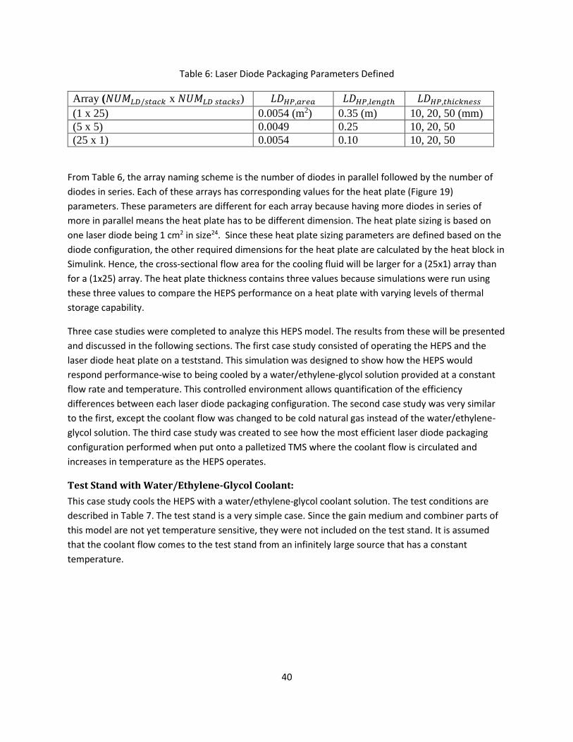
40

Table 6: Laser Diode Packaging Parameters Defined

Array (𝑁𝑈𝑀𝐿𝐷/𝑠𝑡𝑎𝑐𝑘 x 𝑁𝑈𝑀𝐿𝐷 𝑠𝑡𝑎𝑐𝑘𝑠) 𝐿𝐷𝐻𝑃,𝑎𝑟𝑒𝑎 𝐿𝐷𝐻𝑃,𝑙𝑒𝑛𝑔𝑡ℎ 𝐿𝐷𝐻𝑃,𝑡ℎ𝑖𝑐𝑘𝑛𝑒𝑠𝑠

(1 x 25) 0.0054 (m2) 0.35 (m) 10, 20, 50 (mm)

(5 x 5) 0.0049 0.25 10, 20, 50

(25 x 1) 0.0054 0.10 10, 20, 50

From Table 6, the array naming scheme is the number of diodes in parallel followed by the number of

diodes in series. Each of these arrays has corresponding values for the heat plate (Figure 19)

parameters. These parameters are different for each array because having more diodes in series of

more in parallel means the heat plate has to be different dimension. The heat plate sizing is based on

one laser diode being 1 cm2 in size24. Since these heat plate sizing parameters are defined based on the

diode configuration, the other required dimensions for the heat plate are calculated by the heat block in

Simulink. Hence, the cross-sectional flow area for the cooling fluid will be larger for a (25x1) array than

for a (1x25) array. The heat plate thickness contains three values because simulations were run using

these three values to compare the HEPS performance on a heat plate with varying levels of thermal

storage capability.

Three case studies were completed to analyze this HEPS model. The results from these will be presented

and discussed in the following sections. The first case study consisted of operating the HEPS and the

laser diode heat plate on a teststand. This simulation was designed to show how the HEPS would

respond performance-wise to being cooled by a water/ethylene-glycol solution provided at a constant

flow rate and temperature. This controlled environment allows quantification of the efficiency

differences between each laser diode packaging configuration. The second case study was very similar

to the first, except the coolant flow was changed to be cold natural gas instead of the water/ethylene-

glycol solution. The third case study was created to see how the most efficient laser diode packaging

configuration performed when put onto a palletized TMS where the coolant flow is circulated and

increases in temperature as the HEPS operates.

Test Stand with Water/Ethylene-Glycol Coolant:

This case study cools the HEPS with a water/ethylene-glycol coolant solution. The test conditions are

described in Table 7. The test stand is a very simple case. Since the gain medium and combiner parts of

this model are not yet temperature sensitive, they were not included on the test stand. It is assumed

that the coolant flow comes to the test stand from an infinitely large source that has a constant

temperature.

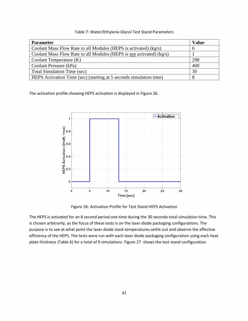
41

Table 7: Water/Ethylene-Glycol Test Stand Parameters

Parameter Value

Coolant Mass Flow Rate to all Modules (HEPS is activated) (kg/s) 6

Coolant Mass Flow Rate to all Modules (HEPS is not activated) (kg/s) 1

Coolant Temperature (K) 298

Coolant Pressure (kPa) 400

Total Simulation Time (sec) 30

HEPS Activation Time (sec) (starting at 5 seconds simulation time) 8

The activation profile showing HEPS activation is displayed in Figure 26.

Figure 26: Activation Profile for Test Stand HEPS Activation

The HEPS is activated for an 8 second period one time during the 30 seconds total simulation time. This

is chosen arbitrarily, as the focus of these tests is on the laser diode packaging configurations. The

purpose is to see at what point the laser diode stack temperatures settle out and observe the effective

efficiency of the HEPS. The tests were run with each laser diode packaging configuration using each heat

plate thickness (Table 6) for a total of 9 simulations. Figure 27 shows the test stand configuration.

42

Figure 27: Test Stand Configuration for Water/Ethylene-Glycol Cooling Fluid

The results of this case study are presented next. The optical power out of each diode array

configuration for each heat plate thickness is exhibited for easy observation of the most efficient

configuration. Other supporting data follows to confirm the test stand is operating within the laws of

Thermodynamics. Figure 28 is the optical power out of the HEPS based on three laser diode array

configurations over the entire mission profile for a heat plate thickness of 10 mm.

Figure 28: Optical Power of Laser Diode Configurations Cooled with Water/Ethylene-Glycol (Full and

Zoomed View, Heat Plate Thickness = 10mm)

43

The optical power output is 0 during the time when the HEPS is not activted, as is expected. Notice how

the optical power starts at a maximum point the moment the HEPS acivates and decreases as the HEPS

activation continues. The moment the HEPS activates, this is the maximum optical power that can

possibly be produced by the HEPS. At anytime after this, the temperature of the laser diode stacks is no

longer equal to the laser diode reference temperature. This temperature difference causes the

wavelength shift described earlier, which decreases the optical power absorbed by the gain medium.

The optical power out of the HEPS for all three heat plate thicknesses is shown in Figure 29.

Figure 29: Optical Power During HEPS Activation Cooled with Water/Ethylene-Glycol for Heat Plate

Thicknesses (10, 20, and 50 mm)

A thicker heat plate means more thermal storage is available. This, in turn, means the laser diode stack

temperatures do not rise as fast over the period of HEPS activation. The temperatures are more

controlled, and hence the optical power out of the HEPS does not decrease as fast during activation. This

optical power data leads to quantifying the effective efficiency of the HEPS (refer to equation 6),

displayed in Figure 30.

44

Figure 30: Effective Efficiency during HEPS Activation Cooled with Water/Ethylene-Glycol for Heat Plate

Thicknesses (10, 20, and 50 mm)

The effective efficiency takes into account that a HEPS has a maximum amount of optical power it can

output given absolutely perfect operating conditions, meaning all the laser diode stack temperatures

stay equal to the laser diode reference temperature for the duration of the HEPS activation time. This

optical power output value is compared to all the other optical output values and an efficiency is

calculated. The effective efficiency should be as close to 100% as possible for the duration of HEPS

activation to achieve the highest optical power output. As seen in Figure 30, the (1x25) array gives the

highest effective efficiency for every plate thickness, followed by the (5x5) array and then the (25x1)

array. For all thicknesses, the same laser diode configuration will eventually settle out to the same

efficiency value if activation time were extended long enough for steady-state operation. The extra

thermal storage simply increases the time to reach this steady state efficiency.

Another way of looking at this data is to observe the energy output from the HEPS over the activation

time period. This is simply done by taking the integral of the curves in Figure 29. Quantifying the area

under each of these curves gives an equally valuable method of analysis for understanding how and why

what laser diode configuration is the most efficient. Table 8 contains the energy output data for each

laser diode configuration during the HEPS activation period.

45


Configurations Ranked Best to Worst (Water/Ethylene-Glycol)

Heat Plate Thickness (mm) Array Energy Out of HEPS (kJ) Ranking

10

(1x25) 710.5 1

(5x5) 620.2 2

(25x1) 326.0 3

20

(1x25) 720.6 1

(5x5) 665.8 2

(25x1) 516.6 3

50

(1x25) 744.8 1

(5x5) 733.7 2

(25x1) 706.2 3

The (1x25) laser diode configuration has the most energy output for each heat plate thickness. Notice

how as the amount of thermal storage increases (thicker heat plate), the range of the energy output

values for the three laser diode configurations decreases. Again, the same laser diode configuration will

eventually settle out to the same efficiency value. The extra thermal storage simply increases the time

to reach this steady state efficiency.

It is of paramount importance to make sure the results shown above are thermally valid. This is

accomplished by analyzing coolant flow parameters into, out of, and within the laser diode heat plate

for each laser diode configuration. Remembering that the heat plate is divided up into 𝑁𝑈𝑀𝐿𝐷 𝑠𝑡𝑎𝑐𝑘𝑠

discrete volumes, the Reynold’s Number (Re) and convective heat transfer coefficient (h) at each of

these discrete volumes should be observed to know whether or not they are reasonable values given

the type of coolant and coolant flow rate. Table 7 gave a coolant flow rate of 6 kg/s. Notice that since

there are 40 modules, each heat plate actually sees a coolant flow of 0.15 kg/s when the HEPS is

activated. With this in mind, data for the coolant flow within the heat plate for the (25x1) array is


46


Thickness = 10 mm

There is only one laser diode stack in this configuration, so the one curve on each graph represents the

solitary discrete volume. With this configuration, the cross sectional area of the coolant flow is larger.

This should yield a small fluid velocity through the heat plate, which in turn should yield a relatively

small Reynold’s Number. From Figure 31, the Reynold’s Number peaks at around 1500. For a fluid like

water/ethylene glycol moving through an internal passage with the dimensions described in Table 6, this

is a reasonable value. This small Reynold’s Number yields an h value of around 0.9 W/cm2 K. Given the

Gnielinksi Correlations utilized by the heat plate calculations, this is a reasonable value with a working

fluid of water/ethylene-glycol. The single laser diode stack temperature shown has increased around

70K by the end of HEPS activation time when compared to the laser diode reference temperature of

298K. In looking at the other two laser diode configurations, the trends of these values can be observed.

From these trends, their validity can be better established. As the number of discrete volumes increases,

the amount of heat seen by each discrete volume decreases since the total amount of heat produced by

the laser diodes stays constant for each laser diode configuration. Figure 32 shows data for the coolant

flow within the heat plate for the (5x5) array.

47


Thickness = 10 mm

There are five laser diode stacks in this configuration, so the the Re and h values are evaluated locally at

the five discrete volumes of the heat plate. With this configuration, the cross sectional area of the

coolant flow is smaller than the (25x1) array. This should yield a larger fluid velocity through the heat

plate, which in turn should yield a relatively larger Reynold’s Number. In Figure 32, the Reynold’s

Number range is from around 3500 to 4000. For a fluid like water/ethylene-glycol moving through an

internal passage with the dimensions described in Table 6, this is a reasonable value. This larger range of

Reynold’s Numbers yields an h value range from around 3.9 to 4.7 W/cm2 K. Given the Gnielinksi

Correlations utilized by the heat plate calculations, this is a reasonable value with a working fluid of

water/ethylene-glycol. Because the cross sectional area for the coolant flow is smaller here than for the

(25x1) array, larger local Reynold’s Numbers (and therefore larger local h values) are to be expected.

Larger local h values coupled with a smaller amount of heat applied to each discrete volume means the

laser diode stack temperatures do not increase near as much when compared with the (25x1) diode

configuration in Figure 31. The data for the coolant flow within the heat plate for the (1x25) diode

configuration is displayed in Figure 33.

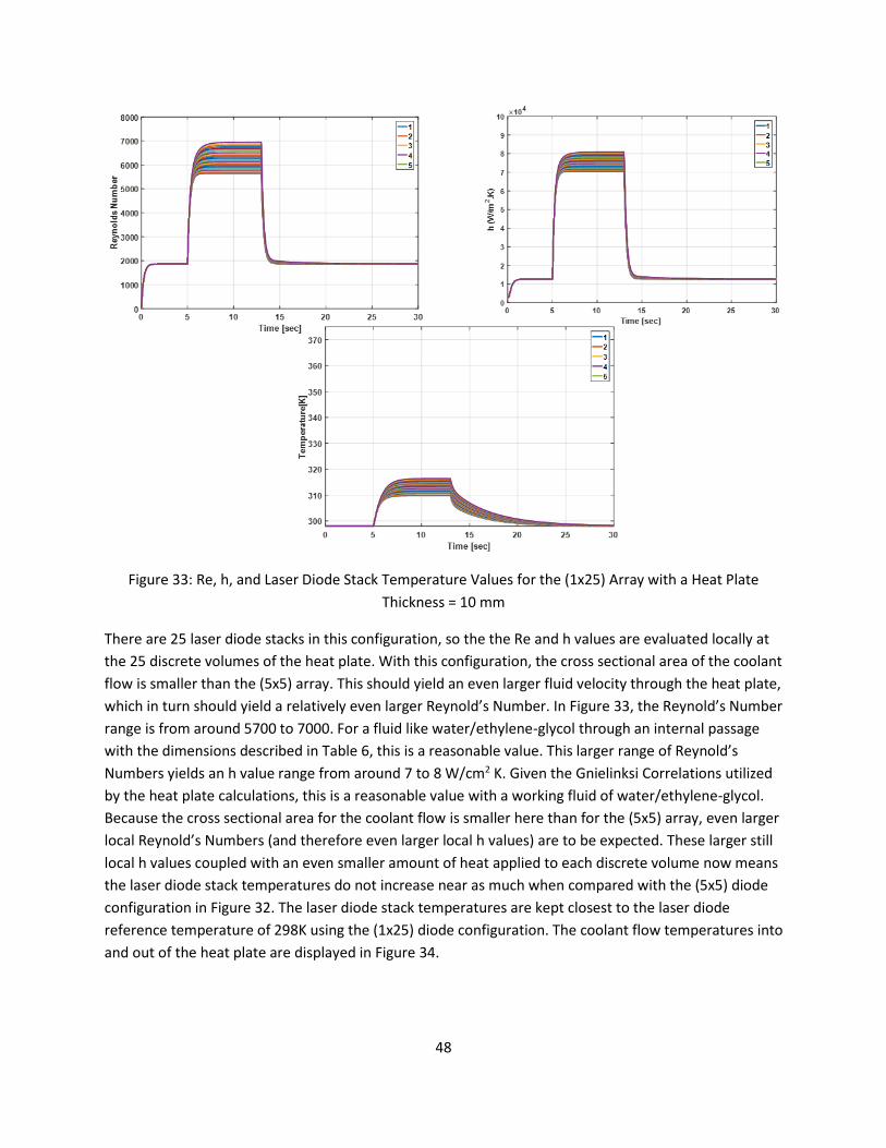
48


Thickness = 10 mm

There are 25 laser diode stacks in this configuration, so the the Re and h values are evaluated locally at

the 25 discrete volumes of the heat plate. With this configuration, the cross sectional area of the coolant

flow is smaller than the (5x5) array. This should yield an even larger fluid velocity through the heat plate,

which in turn should yield a relatively even larger Reynold’s Number. In Figure 33, the Reynold’s Number

range is from around 5700 to 7000. For a fluid like water/ethylene-glycol through an internal passage

with the dimensions described in Table 6, this is a reasonable value. This larger range of Reynold’s

Numbers yields an h value range from around 7 to 8 W/cm2 K. Given the Gnielinksi Correlations utilized

by the heat plate calculations, this is a reasonable value with a working fluid of water/ethylene-glycol.

Because the cross sectional area for the coolant flow is smaller here than for the (5x5) array, even larger

local Reynold’s Numbers (and therefore even larger local h values) are to be expected. These larger still

local h values coupled with an even smaller amount of heat applied to each discrete volume now means

the laser diode stack temperatures do not increase near as much when compared with the (5x5) diode

configuration in Figure 32. The laser diode stack temperatures are kept closest to the laser diode

reference temperature of 298K using the (1x25) diode configuration. The coolant flow temperatures into

and out of the heat plate are displayed in Figure 34.

49

Figure 34: Water/Ethylene-Glycol In and Out Temperatures for the Three Diode Configuraitons with a

Heat Plate Thickness = 10 mm

The temperatures of the coolant flow going into and coming out of the heat plate shown here provide

insight into how the coolant temperature is changing from the heat plate inlet to exit throughout the

HEPS activation time. Remember the flow rate to all modules is 6 kg/s when the HEPS is activated and 1

kg/s when the HEPS is not activated. This explains the behavior exhibited by each diode configuration in

the moments after the HEPS is deactivated. As the number of discrete volume decreases, the amount of

heat seen by each discrete volume increases. Hence, the (25x1) configuration has lots of heat to get rid

of from the single discrete volume. This is why the temperature dips the way it does. The flow rate

changing from 6 kg/s to 1 kg/s means the coolant flow out actually increases in temperature before it

begins to drop again because it is absorbing all the residual heat from the single discrete volume. This is

not seen in the (5x5) and (1x25) configurations because the residual heat in each discrete volume is not

large enough to have this effect.

The coolant flow data presented above is very similar for the cases with heat plate thicknesses of 20 and

50 mm. The only difference is that the Re and h values take a little longer to reach steady state when the

flow rate changes due to HEPS activation. The additional thermal storage capability also means the laser

diode stack temperatures also take longer to reach steady state. Over a constant period of HEPS

activation time (8 seconds), the laser diode stack temperatures show less of a change from the laser

50

diode reference temperature. This leads to the better efficiency values observed for a larger thermal

mass for the same amount of HEPS activation time in Figure 30.

Test Stand with Cold Natural Gas Coolant:

This case study is very similar to the one described above, but the HEPS is now cooled with cold natural

gas (CNG). The test conditions are described in Table 9.

Table 9: CNG Test Stand Parameters

Parameter Value

Coolant Mass Flow Rate to all Modules (HEPS is activated) (kg/s) 1.5

Coolant Mass Flow Rate to all Modules (HEPS is not activated) (kg/s) 0.25

Coolant Temperature (HEPS is activated) (K) 230

Coolant Temperature (HEPS is not activated) (K) 290

Coolant Pressure (kPa) 300

Total Simulation Time (sec) 30

HEPS Activation Time (starting at 5 seconds simulation time) (sec) 8

CNG was chosen for a comparison to the water/ethylene-glycol solution. Testing both a liquid and a gas

provides valuable data on the thermal capabilities of each one. Certain laser diode configurations may

be more efficient than others depending on the cooling fluid used. The differing properties between a

water/ethylene-glycol solution and CNG may control the laser diode stack temperatures in a different

manner. The lower density of the CNG will cause it to heat up faster when compared with the

water/ethylene-glycol solution. However, the larger temperature differential between the laser diode

stacks and the CNG might yield better temperature control. Notice how the CNG flow in temperature

becomes colder when the HEPS is activated, which is different from the water/ethylene-glycol test stand

where the coolant flow in stayed the same temperature regardless of whether or not the HEPS was

activated. This simple case using a test stand has the means to provide data for observing trends in HEPS

efficiency for both cooling fluids. Since the gain medium and combiner parts of this model are not yet

temperature sensitive, they were not included on this test stand either. It is assumed that the CNG

coolant flow comes to the test stand from an infinitely large source that has a constant temperature.

The profile showing HEPS activation is the same as for the water/ethylene-glycol tests displayed in

Figure 26. Again, this mission profile is chosen arbitrarily, as the focus of these tests is on the laser diode

packaging configurations. The purpose is to see at what point the laser diode stack temperatures settle

out and observe the effective efficiency of the HEPS. The tests were run with each laser diode packaging

configuration using each heat plate thickness (Table 6) for a total of 9 simulations. Figure 35 shows the

test stand configuration using CNG.

51

Figure 35: Test Stand Configuration for Cold Natural Gas Cooling Fluid

The CNG was modeled as pure Methane in the test stand. The optical power out of each diode array

configuration for each heat plate thickness is exhibited for easy observation of the most efficient

configuration. Other supporting data follows to confirm the test stand is operating within the laws of

Thermodynamics. Figure 36 is the optical power out of the HEPS based on three laser diode array

configurations over the entire mission profile for a heat plate thickness of 10 mm.

Figure 36: Optical Power of Laser Diode Configurations Cooled with CNG (Full and Zoomed View, Heat

Plate Thickness = 10mm)

52

The optical power output is 0 during the time when the HEPS is not activted, as is expected. Notice how

the optical power starts at a maximum point the moment the HEPS acivates and decreases as the HEPS

activation continues. The moment the HEPS activates, this is the maximum optical power that can

possibly be produced by the HEPS. At anytime after this, the temperature of the laser diode stacks is no

longer equal to the laser diode reference temperature. This temperature difference causes the

wavelength shift described earlier, which decreases the optical power absorbed by the gain medium.

The optical power out of the HEPS for all three heat plate thicknesses is shown in Figure 37.

Figure 37: Optical Power During HEPS Activation Cooled with CNG for Heat Plate Thicknesses (10, 20,

and 50 mm)

A thicker heat plate means more thermal storage is available. This, in turn, means the laser diode stack

temperatures do not rise as fast over the period of HEPS activation. The temperatures are more

controlled, and hence the optical power out of the HEPS does not decrease as fast during activation. This

optical power data leads to quantifying the effective efficiency of the HEPS (refer to equation 6),


53

Figure 38: Effective Efficiency during HEPS Activation Cooled with CNG for Heat Plate Thicknesses (10,

20, and 50 mm)

The effective efficiency takes into account that a HEPS has a maximum amount of optical power it can

output given absolutely perfect operating conditions, meaning all the laser diode stack temperatures

stay equal to the laser diode reference temperature for the duration of the HEPS activation time. Again,

this optical power output value is compared to all the other optical output values and an efficiency is

calculated. The effective efficiency should be as close to 100% as possible for the duration of HEPS

activation to achieve the highest optical power output. As shown in Figure 38, the (5x5) array gives the

highest effective efficiency for every plate thickness. The (1x25) array has the next highest efficiency for

the 10 and 20 mm heat plate thickness, but it falls to third place for the 50 mm plate thickness as the

(25x1) array has the second-best efficiency for the 50 mm heat plate thickness. For all heat plate

thicknesses, the same laser diode configuration will eventually settle out to the same efficiency value.

The extra thermal storage simply increases the time to reach this steady state efficiency.

Another way of looking at this data is to observe the energy output from the HEPS over the activation

time period. This is simply done by taking the integral of the curves in Figure 37. Quantifying the area

under each of these curves gives an equally valuable method of analysis for understanding how and why

which laser diode configuration is the most efficient. Table 10 contains the energy output data for each

laser diode configuration during the HEPS activation period.

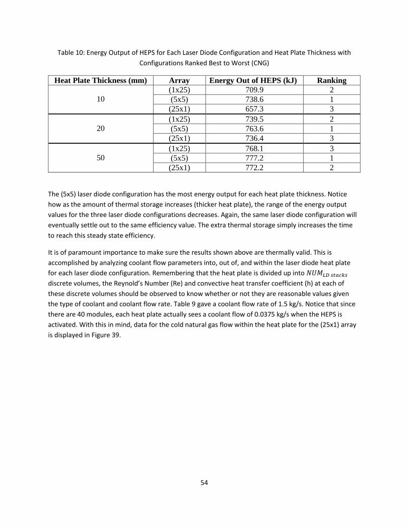
54


Configurations Ranked Best to Worst (CNG)

Heat Plate Thickness (mm) Array Energy Out of HEPS (kJ) Ranking

10

(1x25) 709.9 2

(5x5) 738.6 1

(25x1) 657.3 3

20

(1x25) 739.5 2

(5x5) 763.6 1

(25x1) 736.4 3

50

(1x25) 768.1 3

(5x5) 777.2 1

(25x1) 772.2 2

The (5x5) laser diode configuration has the most energy output for each heat plate thickness. Notice

how as the amount of thermal storage increases (thicker heat plate), the range of the energy output

values for the three laser diode configurations decreases. Again, the same laser diode configuration will

eventually settle out to the same efficiency value. The extra thermal storage simply increases the time

to reach this steady state efficiency.

It is of paramount importance to make sure the results shown above are thermally valid. This is

accomplished by analyzing coolant flow parameters into, out of, and within the laser diode heat plate

for each laser diode configuration. Remembering that the heat plate is divided up into 𝑁𝑈𝑀𝐿𝐷 𝑠𝑡𝑎𝑐𝑘𝑠

discrete volumes, the Reynold’s Number (Re) and convective heat transfer coefficient (h) at each of

these discrete volumes should be observed to know whether or not they are reasonable values given

the type of coolant and coolant flow rate. Table 9 gave a coolant flow rate of 1.5 kg/s. Notice that since

there are 40 modules, each heat plate actually sees a coolant flow of 0.0375 kg/s when the HEPS is

activated. With this in mind, data for the cold natural gas flow within the heat plate for the (25x1) array

is displayed in Figure 39.

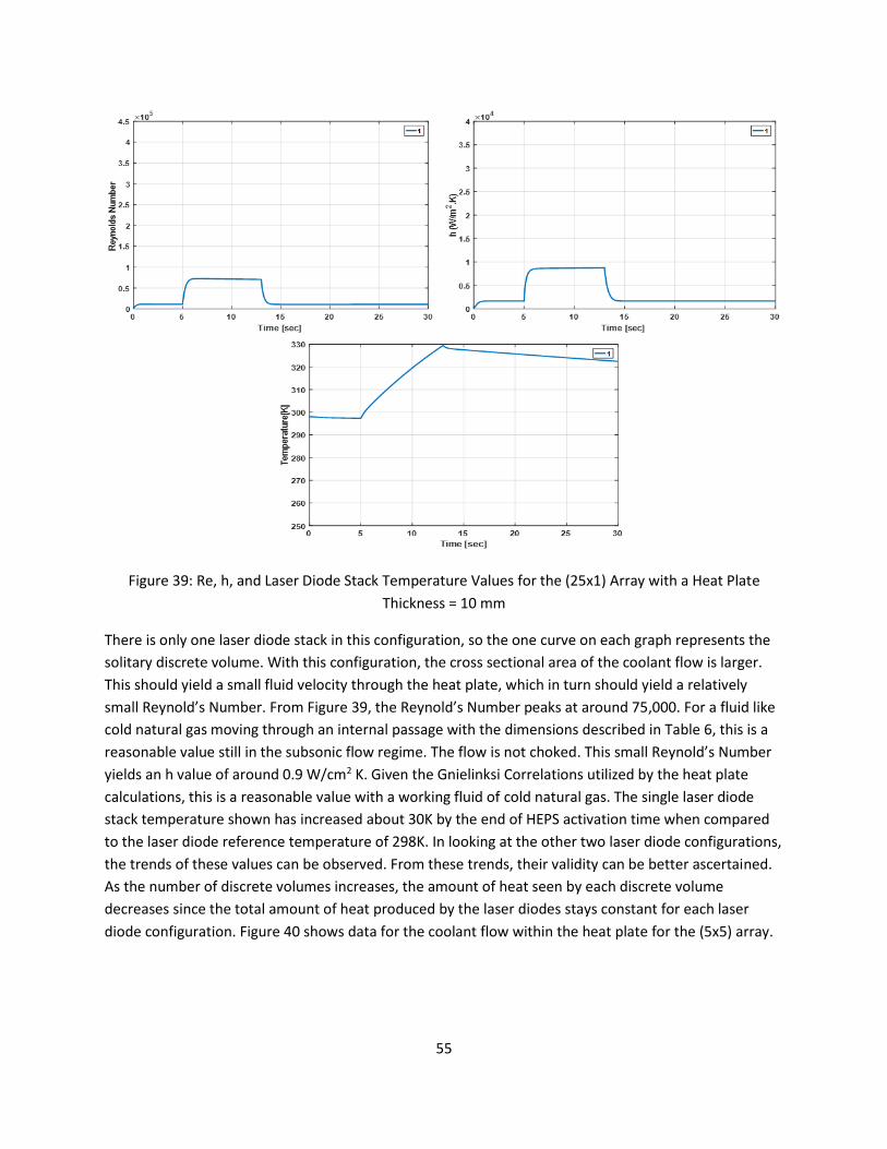
55


Thickness = 10 mm

There is only one laser diode stack in this configuration, so the one curve on each graph represents the

solitary discrete volume. With this configuration, the cross sectional area of the coolant flow is larger.

This should yield a small fluid velocity through the heat plate, which in turn should yield a relatively

small Reynold’s Number. From Figure 39, the Reynold’s Number peaks at around 75,000. For a fluid like

cold natural gas moving through an internal passage with the dimensions described in Table 6, this is a

reasonable value still in the subsonic flow regime. The flow is not choked. This small Reynold’s Number

yields an h value of around 0.9 W/cm2 K. Given the Gnielinksi Correlations utilized by the heat plate

calculations, this is a reasonable value with a working fluid of cold natural gas. The single laser diode

stack temperature shown has increased about 30K by the end of HEPS activation time when compared

to the laser diode reference temperature of 298K. In looking at the other two laser diode configurations,

the trends of these values can be observed. From these trends, their validity can be better ascertained.

As the number of discrete volumes increases, the amount of heat seen by each discrete volume

decreases since the total amount of heat produced by the laser diodes stays constant for each laser

diode configuration. Figure 40 shows data for the coolant flow within the heat plate for the (5x5) array.

56


Thickness = 10 mm

There are five laser diode stacks in this configuration, so the the Re and h values are evaluated locally at

the five discrete volumes of the heat plate. With this configuration, the cross sectional area of the

coolant flow is smaller than the (25x1) array. This should yield a larger fluid velocity through the heat

plate, which in turn should yield a relatively larger Reynold’s Number. In Figure 40, the Reynold’s

Number range is from around 190,000 to 210,000. For a fluid like cold natural gas moving through an

internal passage with the dimensions described in Table 6, this is a reasonable value. The Reynold’s

Number is decreasing at each discrete volume along the heat plate because the viscosity of a gas

increases as its temperature increases, and the fluid velocity increase due to heat addition is not enough

to counteract. This larger range of Reynold’s Numbers yields an h value range from around 1.9 to 2

W/cm2 K. Given the Gnielinksi Correlations utilized by the heat plate calculations, this is a reasonable

value with a working fluid of cold natural gas. Because the cross sectional area for the coolant flow is

smaller here than for the (25x1) array, larger local Reynold’s Numbers (and therefore larger local h

values) are to be expected. Larger local h values coupled with a smaller amount of heat applied to each

discrete volume means the laser diode stack temperatures do not increase near as much when

compared with the (25x1) diode configuration in Figure 39. The data for the coolant flow within the heat

plate for the (1x25) diode configuration is displayed in Figure 41.

57


Thickness = 10 mm

There are 25 laser diode stacks in this configuration, so the the Re and h values are evaluated locally at

the 25 discrete volumes of the heat plate. With this configuration, the cross sectional area of the coolant

flow is smaller than the (5x5) array. This should yield an even larger fluid velocity through the heat plate,

which in turn should yield a relatively even larger Reynold’s Number. In Figure 41, the Reynold’s Number

range is from around 330,000 to 400,000. For a fluid like cold natural gas moving through an internal

passage with the dimensions described in Table 6, this is a reasonable value. This larger range of

Reynold’s Numbers yields an h value range from around 3 to 3.4 W/cm2 K. Given the Gnielinksi

Correlations utilized by the heat plate calculations, this is a reasonable value with a working fluid of cold

natural gas. These values should be much lower than that of water/ethylene-glycol, and indeed they are.

Because the cross sectional area for the coolant flow is smaller here than for the (5x5) array, even larger

local Reynold’s Numbers (and therefore even larger local h values) are to be expected. These larger still

local h values coupled with an even smaller amount of heat applied to each discrete volume now means

the laser diode stack temperatures do not increase near as much when compared with the (5x5) diode

configuration in Figure 40. In fact, some stack temperatures drop below the laser diode reference

temperature as seen in Figure 41. The laser diode stack temperatures are not kept closer to the laser

diode reference temperature of 298K using the (1x25) diode configuration when compared to the (5x5)

configuration. The coolant flow temperatures into and out of the heat plate are displayed in Figure 42.

58

Figure 42: CNG In and Out Temperatures for the Three Diode Configuraitons with a Heat Plate Thickness

= 10 mm

The temperatures of the coolant flow going into and coming out of the heat plate shown here provide

insight into how the coolant temperature is changing from the heat plate inlet to exit throughout the

HEPS activation time. Remember the flow rate to all modules is 1.5 kg/s when the HEPS is activated and

0.25 kg/s when the HEPS is not activated. This explains the behavior exhibited by each diode

configuration in the moments after the HEPS is activated. The flow is in contact with the heat plate for

more time in the (1x25) configuration, it has more of a chance to heat up by the time it exits. The (25x1)

configuration provides less time for the CNG to be in contact with the heat plate, so the outlet

temperature of the flow is closer to the inlet temperature of the flow for this diode configuration during

HEPS activation.

The coolant flow data presented above is very similar for the cases with heat plate thicknesses of 20 and

50 mm. The only difference is that the Re and h values take a little longer to reach steady state when the

flow rate changes due to HEPS activation. The additional thermal storage capability also means the laser

diode stack temperatures also take longer to reach steady state. Over a constant period of HEPS

activation time (8 seconds), the laser diode stack temperatures show less of a change from the laser

diode reference temperature. This leads to the better efficiency values observed for a larger thermal

mass for the same amount of HEPS activation time as shown in Figure 38.

59

Test Stand Results Discussion:

The test stand cases are intriguing because the results show several interesting performance

characteristics. In using the dynamic efficiency HEPS model, the difference in effective efficiency

between laser diode array configurations was observed. Since the temperature of the laser diode stacks

is now connected to the optical power output via the wavelength shift, the model showed changing

optical power output as the HEPS operated for its 8 second time period.

Using the water/ethylene-glycol fluid, the (1x25) array had the best effective efficiency, followed by the

(5x5) array and then lastly by the (25x1) array. This is significant because it shows there is actually a

configuration of diode arrangement that yields the best effective efficiency. The best laser diode stack

temperature control occurs when the diodes are in series thermally. Mounting the diode stacks to a

thicker heat plate shows the effect of thermal storage on effective efficiency. A larger thermal storage

capability yields a slower increase in laser diode stack temperature over the same HEPS activation

period of 8 seconds. The stacks will still reach the same steady state temperature with more thermal

storage versus less. However, with more thermal storage, it takes longer to reach the steady state

temperature. This is both advantageous and detrimental. A larger thermal storage capability in this

setup also means more cooling capacity is needed to bring the laser diode stacks back to the diode

reference temperature. This is a trade off in that a larger thermal storage means the diode stack

temperature do not increase as fast yet need more cooling capacity, while a smaller thermal storage

means the diode stack temperatures increase faster yet do not need as much cooling capacity to bring

the temperatures back to the reference set point. Either one of these (larger or smaller thermal storage)

could be applicable depending on the TMS type/design used to cool the HEPS, as there are situations

where each style could be advantageous to utilize.

The flow rate of water/ethylene-glycol to the laser diode heat plates will now be investigated. There is a

total flow of 6 kg/s to all 40 modules, so each module sees 0.15 kg/s of coolant flow. The incoming flow

has to be split 40 different directions for use in all the heat plates. Having all this flow in parallel yields

the need for a very large manifold in a real-life system to deliver the coolant where it needs to go. This

large manifold, along with the laser diode heat plate, yields very large pressure drops in the system. A

higher number of laser diode stacks in series (1x25) yields a higher pressure drop across all 40 of the

heat plates. These factors combine to yield potential pressure drops on the order of Mega-Pascals,

which would require very large pumps in terms of both mass and volume. Even with a flow of 6 kg/s to

all modules, the diode stack temperatures are not kept close to the reference temperature. This means

even higher pressure drops will occur if the flow rate is higher. Clearly, this shows how challenging the

TMS design requirements could be for a HEPS with an optical output on the order of 100 kW.

Using cold natural gas (CNG) as the coolant in the test stand provides a good comparison to the

water/ethylene-glycol results. CNG differs in several ways. It is a gas, so it is much less dense than the

water/ethylene-glycol solution. It is flowing at a temperature of 230K versus the 298K of the

water/ethylene-glycol solution. The flow rate of the CNG during HEPS activation is also significantly less

60

at 1.5 kg/s to all modules (0.0375 kg/s to each module). For CNG, the (5x5) array had the best effective

efficiency, followed by the (1x25) array and then lastly by the (25x1) array during the HEPS activation

period of 8 seconds. These effective efficiencies are higher than the ones observed in the

water/ethylene-glycol solution test stand case. A larger thermal storage again shows much better

effective efficiency values.

The optimal diode configuration is different between the two test stand cases, (1x25) for

water/ethylene-glycol and (5x5) for CNG. This is significant as it shows there may be a different optimal

diode configuration for various cooling fluids at various flow temperatures. For CNG, the high difference

in temperature drives the heat transfer rate from the diode stacks. For water/ethylene-glycol, the higher

heat transfer coefficients drive the heat transfer rate from the diode stacks. The high temperature

difference for the CNG means it can provide better heat transfer and temperature control of the diode

stacks using a significantly lower flow rate to the laser diode heat plates. Overall, a HEPS cooled with

CNG would use less coolant during operation. Storing the required LNG uses much less mass and volume

than storing the required water/ethylene-glycol solution. There are cryogenic complexities not taken

into account in these test stand simulations about going to from LNG to CNG. The LNG must either be

heated, or the pressure must drop dramatically for the liquid to boil and become a cold gas. In order to

effectively and consistently cool the large heat loads from a HEPS, CNG could be a viable solution when

compared to cooling with a more traditional fluid like water/ethylene-glycol based on the test stand

results.

Palletized System with Water/Ethylene-Glycol Coolant:

This case study uses the palletized TMS shown in Figure 25. It is a much more complex simulation in that

now the HEPS performance is being examined coupled to a TMS. The goal is to observe the power-

thermal interactions betweenn the HEPS and TMS to see the differences in performance between the

previous constant efficiency HEPS model3,25 and the dynamic efficiency HEPS model already presented.

First, a case is presented with a constant efficiency HEPS model on the palletized TMS. This is very

similar to Butt25, but the constant efficiency of the HEPS is different from what was in the AIAA paper.

For this simulation, the laser diode, gain medium, and combiner efficiencies were given different values,

as shown in Table 11. The HEPS model has a constant electrical to optical efficiency of 32%, so it would

match the maximum optical efficiency possible out of the dynamic HEPS model. This gives a good basis

for comparing performance.

61

Table 11: HEPS Component Efficiencies and Values for Constant Efficiency Simulation

Parameter Value

Laser Diode Efficiency 0.48

Gain Medium Efficiency 0.78

Combiner Efficiency 0.85

Electrical Power to HEPS (kW) 306

Optical Power Out of HEPS (kW) 97

Thermal Load from Laser Diodes (kW) 159

Thermal Load from Gain Medium (kW) 33

Thermal Load from Combiner (kW) 17

Total Thermal Load from HEPS (kW) 209

The values in Table 11 stay the same throughout HEPS activation. The combiner efficiency is the

efficiency of three components: Beam Director, Mirrors, and Aperture Sharing Element. The efficiency

values for each of these individual components are set to 95%, 97%, and 92% respectively. This yields an

overall combiner efficiency of 85%. The activation profile showing HEPS activation for the palletized TMS

simulation is given in Figure 43.

Figure 43: Activation Profile for Palletized HEPS Simulations

The total time for this activation profile is 600 seconds. A 10% duty cycle was chosen, yielding a total

HEPS activation time for the activation profile of 60 seconds. The HEPS activation periods occur every 40

seconds with 4 seconds of actual activation time. The first HEPS activation occurs at 5 seconds into the

62

mission to allow some time for the TMS to power up and settle out, and the subsequent activations

occur at every 40 seconds thereafter.

Figure 44 displays the optical power out the HEPS for the entire time period of 600 seconds.

Figure 44: Optical Power out of Constant Efficiency HEPS for Palletized TMS Simulation

The optical power out follows the activation profile in Figure 43. It is constant during each activation and

throughout all activations. This is expected as the HEPS efficiency is kept constant for this simulation.

Figure 45 shows the thermal and electrical power produced and used by the HEPS.

63

Figure 45: Thermal and Electrical Power of Constant Efficiency HEPS for Palletized TMS Simulation

This is provided to show that the system is indeed functioning properly during the simulation and that

the thermal loads are being accounted for. It’s important to show information like this in order to prove

the simulation is actually doing the calculations properly. Another important area of the palletized

system’s performance is the parameters of the cold and hot storage tanks for the coling fluid (see Figure

25). The cold and hot tank fluid masses and flow rates are given below in Figures 46 and 47.

Figure 46: Cold Tank Parameters of Constant Efficiency HEPS for Palletized TMS Simulation

64

Figure 47: Hot Tank Parameters of Constant Efficiency HEPS for Palletized TMS Simulation

The flow rate from the cold tank is 6 kg/s when the state flow conditions are met (HEPS is activated),

and the flow rate from the hot tank is 0.6 kg/s when the state flow conditions are met. From Figures 46

and 47, it can be seen how the flow rates from each tank change throughout the 600 seconds.

Remember, the cold tank flow goes to cool the HEPS, and the hot tank flow goes to the heat exchanger

to be cooled by the CNG. The overall mass of coolant in the cold tank is decreasing throughout the 600

seconds, while the amount in the hot tank increasing. By the end, most of the coolant mass in now

located in the hot tank. Figure 48 below shows the average tank temperatures.

65

Figure 48: Tank Temperatures of Constant Efficiency HEPS for Palletized TMS Simulation

The flow out of the cold tank is meant to stay close to a temperature of 285K for the entire 600 seconds.

A constant temperature coolant flow to the HEPS is very important for operation. This is accomplished

by choosing a set point for the CNG flow temperature around the loop in Figure 25 of 244K. This 244K is

the temperature of the CNG when it comes out of the mixing chamber on it’s way to cool the ethylene-

glycol solution moving from the hot tank to the cold tank.

With the constant efficiency HEPS data presented, the dynamic efficiency HEPS data can be presented

and compared. The baseline results above show the palletized system operation with a constant HEPS

efficiency. The dynamic efficiency HEPS model is put onto this exact same palletized system so the

performance of each HEPS model can be directly compared. The parameter values for all the variables in

the dynamic HEPS model are the same as shown in Tables 5 and 6 using a laser diode packaging array of

(5x5). This means 5 diodes in parallel and 5 in series for each module. The activation profile for this

simulation is the same as in Figure 43. In the dynamic efficiency HEPS model, the temperature of the

laser diodes is taken into account. So, when the laser diode temperature moves away from its reference

temperature, the heat produced by the gain medium will increase due to the shift in wavelength output

from the laser diodes. This additional heat will be added to the palletized TMS. Also, the laser diode heat

plate is more accurately setup in the dynamic HEPS efficiency model to deal with the specific laser diode

array. Since the heat from the laser diodes is now more accurately accounted for, this could have a

significant effect on performance. Additionally, the laser diodes have a temperature set point (laser

diode reference temperature) they must be cooled to after every activation. To accomplish this, the

state flow control now allows 6 kg/s to flow to the laser diode modules when the HEPS is activated and

when the maximum laser diode temperature exceeds this set point. For the following simulation, this

66

laser diode reference temperature set point is 298K, the same as in Table 5. These differences between

the constant efficiency and dynamic efficiency HEPS models observed when operated on the same

palletized TMS will provide valuable data as to the effect of the dynamic efficiency phenomenon on

system performance. Figure 49 shows the optical power out of the HEPS for the entire time period.

Figure 49: Optical Power out of Dynamic Efficiency HEPS for Palletized TMS Simulation

Immediately, it is noticed how the simulation did not run for the entire 600 seconds This will be

discussed in detail later on when appropriate. Simply put, the cold tank fluid mass dropped to 0 kg

before the end of the 600 seconds. No mass in the cold tank means the palletized TMS cannot continue

to provide coolant to the operating HEPS. Already, this is a significant observation in performance

between the TMS using the constant efficiency HEPS model and the dynamic efficiency HEPS model.

Looking back to Figure 44 and comparing, a major difference can be seen in the optical power output

curves. The optical power out is constant in Figure 44, but not constant in Figure 49 above. This

decrease in optical power out due to laser diode temperature changes was observed in the test stand

simulations. The laser diode temperatures do not settle out during the HEPS activation, so the optical

power out is decreasing during each activation time of 4 seconds. The laser diodes make it back to their

reference temperature of 298 before the next activation because the optical power starts out at its

maximum possible value at each activation. If the laser diodes did not get back to 298K before the next

activation began, the optical power out would start at a lower value. This is the same constant optical

power out value shown in Figure 44. More analysis on the laser diode temperatures will be presented

later. Figure 50 shows the thermal and electrical power produced and used by the HEPS.

67

Figure 50: Thermal and Electrical Power of Dynamic Efficiency HEPS for Palletized TMS Simulation

Notice how the thermal load increases during activation periods. This occurs because of the drop in

optical power in Figure 49. Less optical power out means more heat produced. The dynamic efficiency

aspect of this model is again captured here with this data. Another important area of the palletized

system’s performance is the parameters of the cold and hot storage tanks for the cooling fluid (see

Figure 25). The cold and hot tank fluid masses and flow rates are given below in Figures 51 and 52.

68

Figure 51: Cold Tank Parameters of Dynamic Efficiency HEPS for Palletized TMS Simulation

Figure 52: Hot Tank Parameters of Dynamic Efficiency HEPS for Palletized TMS Simulation

The flow rate from the cold tank is 6 kg/s when the state flow conditions are met (HEPS is activated and

diode temperature is above the set point), and the flow rate from the hot tank is 0.6 kg/s when the state

69

flow conditions are met. From Figures 51 and 52, the flow rates from each tank change. The cold tank

flow goes to cool the HEPS, and the hot tank flow goes to the heat exchanger to be cooled by the CNG.

The overall mass of coolant in the cold tank is decreasing, while the amount in the hot tank is increasing.

By the time the simulation ends (about 250 seconds), all the coolant mass in now located in the hot

tank. The reason the entire activation profile cannot be completed is because the cold tank runs out of

coolant. The pumps need to be on for more time now to make sure the laser diodes get back to the set

point temperature after an activation period. This longer required pump operation time means coolant

is leaving the cold tank at an overall faster rate than with the constant efficiency HEPS model. Hence,

the given palletized TMS cannot run the activation profile to completion for the dynamic HEPS efficiency

model. The TMS must be redesigned in some way to achieve the desired performance. For example, a

larger cold tank would solve this problem. The TMS must be redesigned in some way. Figure 53 below

shows the average tank temperatures.

Figure 53: Tank Temperatures of Dynamic Efficiency HEPS for Palletized TMS Simulation

The flow out of the cold tank is meant to stay close to a temperature of 285K for the entire activation

profile and is kept quite close to this temperature. This is accomplished by choosing a set point for the

CNG flow temperature around the loop in Figure 25 of 250K. This number is different than in the

constant efficiency HEPS case due to the more accurate capture of the heat transfer between the laser

diode stacks and the cooling fluid. This 250K is the temperature of the CNG when it comes out of the

mixing chamber on it’s way to cool the ethylene-glycol solution moving from the hot tank to the cold

tank.

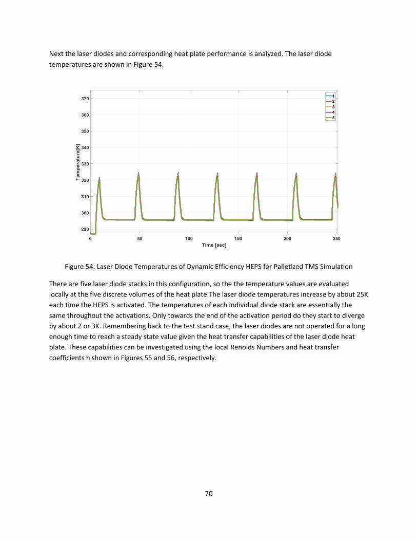
70

Next the laser diodes and corresponding heat plate performance is analyzed. The laser diode

temperatures are shown in Figure 54.

Figure 54: Laser Diode Temperatures of Dynamic Efficiency HEPS for Palletized TMS Simulation

There are five laser diode stacks in this configuration, so the the temperature values are evaluated

locally at the five discrete volumes of the heat plate.The laser diode temperatures increase by about 25K

each time the HEPS is activated. The temperatures of each individual diode stack are essentially the

same throughout the activations. Only towards the end of the activation period do they start to diverge

by about 2 or 3K. Remembering back to the test stand case, the laser diodes are not operated for a long

enough time to reach a steady state value given the heat transfer capabilities of the laser diode heat

plate. These capabilities can be investigated using the local Renolds Numbers and heat transfer

coefficients h shown in Figures 55 and 56, respectively.

71

Figure 55: Reynolds Numbers of Dynamic Efficiency HEPS for Palletized TMS Simulation

Figure 56: Heat Transfer Coefficients of Dynamic Efficiency HEPS for Palletized TMS Simulation

Again, there are five laser diode stacks in this configuration, so the the Reynolds Number and h values

are evaluated locally at the five discrete volumes of the heat plate. The range of Reynolds Numbers

72

during HEPS activation is from about 2200 to 2600, and the range of h values is about 1.9 to 2.6 W/cm2

K. Given 40 modules, each array of laser diodes sees a cooling flow of 0.15 kg/s. This is the same

condition as in the test stand case. Comparing the Reynolds numbers and h values here to the ones in

Figure 32 (Re is 3500 to 4000 and h is 3.9 to 4.7 W/cm2 K) , the values here are between 1.5 and 2 times

smaller than the values in Figure 32. This is a significant difference in heat transfer capability with the

same fluid (water/ethylene-glycol) moving at the same mass flow rate through the heat plate (0.15

kg/s). The difference in heat transfer capability is actually caused by the temperature of the fluid

entering the heat plate. In the test stand case, the fluid is on average 298K at the heat plate (+ or – 2K

based on where the temperature is taken within the heat plate). In the palletized TMS case, the fluid is

on average 287K at the heat plate (+ or – 2K based on where the temperature is taken within the heat

plate). It turns out this temperature difference is the cause of the reduced heat transfer capability, Table

12. The data is based on the temperature ranges observed for the fluid flowing through the laser diode

heat plate in the test stand case of 287K and 298K, respectively.

Table 12: Water/Ethylene-Glycol (60%) Physical Properties at 287K and 298K

Temperature Prandtl

Number

Dynamic

Viscosity

(kg/m s)

Thermal

Conductivity

(W/m K)

Specific Heat

J/kg K

Reynolds

Number

Nusselt

Number

287K 52-40 6.5-4.5e-3 0.358-0.354 3180-3130 2000-

2500

30-42

298K 36-30 4.2 -3.4e-3 0.363-0.359 3110-3060 3500-

4000

50-60

The increase in dynamic visocisty from 298K to 287K yields a decrease in the Reynolds Number, which in

turn yields a decrease in the Nusselt Number. Overall, this shows an overall reduction in heat transfer by

about half from 298K to 287K. This explains the difference in heat transfer coefficent values seen from

the test stand case to the palletized TMS case. Hence, if the HEPS activation period were longer, the

laser diode temperatures in Figure 54 would settle out at a steady state value higher than the steady

state value observed in the test stand case (Figure 32).

A water/ethylene-glycol solution is chosen because it has a lower freezing point than just plain water,

and this is good for the palletized system as it employes the use of cryogenic fluids for cooling that could

take the HEPS coolant fluid below the freezing point of plain water. However, as seen by Table 12, it also

has a large viscosity fluctuation given a relatively small temperature change. This has a negative effect in

the heat transfer capabilities of palletized TMS if the water/ethylene-glycol solution kept at a slightly

colder temperature. Table 13 shows the physical properties given the same temperature change if plain

water was used instead of a water/ethylene-glycol solution (test stand analysis only).

Table 13: Water Physical Properties at 287K and 298K

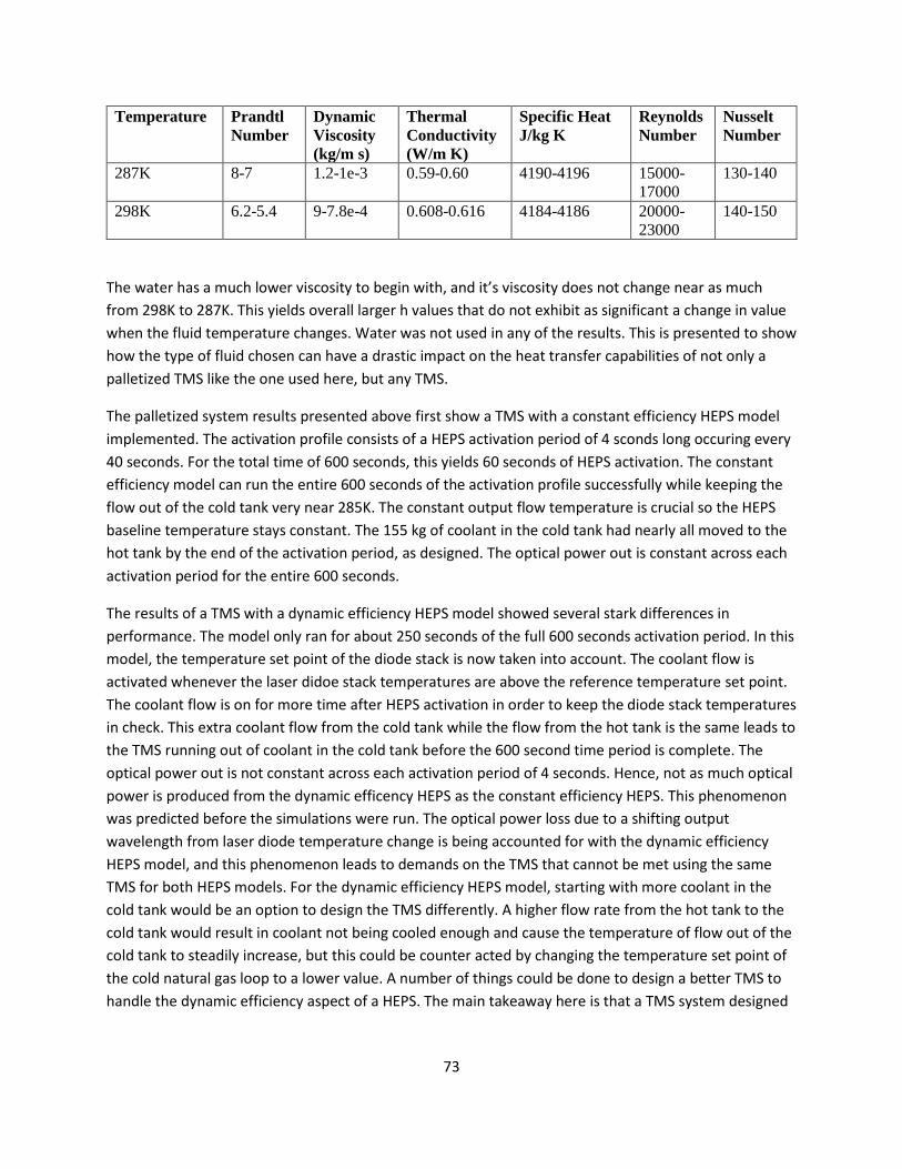
73

Temperature Prandtl

Number

Dynamic

Viscosity

(kg/m s)

Thermal

Conductivity

(W/m K)

Specific Heat

J/kg K

Reynolds

Number

Nusselt

Number

287K 8-7 1.2-1e-3 0.59-0.60 4190-4196 15000-

17000

130-140

298K 6.2-5.4 9-7.8e-4 0.608-0.616 4184-4186 20000-

23000

140-150

The water has a much lower viscosity to begin with, and it’s viscosity does not change near as much

from 298K to 287K. This yields overall larger h values that do not exhibit as significant a change in value

when the fluid temperature changes. Water was not used in any of the results. This is presented to show

how the type of fluid chosen can have a drastic impact on the heat transfer capabilities of not only a

palletized TMS like the one used here, but any TMS.

The palletized system results presented above first show a TMS with a constant efficiency HEPS model

implemented. The activation profile consists of a HEPS activation period of 4 sconds long occuring every

40 seconds. For the total time of 600 seconds, this yields 60 seconds of HEPS activation. The constant

efficiency model can run the entire 600 seconds of the activation profile successfully while keeping the

flow out of the cold tank very near 285K. The constant output flow temperature is crucial so the HEPS

baseline temperature stays constant. The 155 kg of coolant in the cold tank had nearly all moved to the

hot tank by the end of the activation period, as designed. The optical power out is constant across each

activation period for the entire 600 seconds.

The results of a TMS with a dynamic efficiency HEPS model showed several stark differences in

performance. The model only ran for about 250 seconds of the full 600 seconds activation period. In this

model, the temperature set point of the diode stack is now taken into account. The coolant flow is

activated whenever the laser didoe stack temperatures are above the reference temperature set point.

The coolant flow is on for more time after HEPS activation in order to keep the diode stack temperatures

in check. This extra coolant flow from the cold tank while the flow from the hot tank is the same leads to

the TMS running out of coolant in the cold tank before the 600 second time period is complete. The

optical power out is not constant across each activation period of 4 seconds. Hence, not as much optical

power is produced from the dynamic efficency HEPS as the constant efficiency HEPS. This phenomenon

was predicted before the simulations were run. The optical power loss due to a shifting output

wavelength from laser diode temperature change is being accounted for with the dynamic efficiency

HEPS model, and this phenomenon leads to demands on the TMS that cannot be met using the same

TMS for both HEPS models. For the dynamic efficiency HEPS model, starting with more coolant in the

cold tank would be an option to design the TMS differently. A higher flow rate from the hot tank to the

cold tank would result in coolant not being cooled enough and cause the temperature of flow out of the

cold tank to steadily increase, but this could be counter acted by changing the temperature set point of

the cold natural gas loop to a lower value. A number of things could be done to design a better TMS to

handle the dynamic efficiency aspect of a HEPS. The main takeaway here is that a TMS system designed

74

specifically for the constant efficiency HEPS does not have the capability to handle the additional heat

load and control requirements of a dynamic efficiency HEPS.

Conclusions:

Effective cooling of thermal loads generated by advanced electronics is becoming increasingly

challenging as these loads grow larger with the development of new technologies. Advanced electronic

technologies are smaller and lighter. The smaller sizes and higher heat loads mean the temperature

control of these electronics is becoming ever more important, as even small increases in temperature

can render the electronics inoperable. This makes the task of thermal management even more difficult.

A HEPS is one of these such systems. A HEPS is essentially a large laser system. In operating a HEPS with

an optical power output on the order of 100 kW, a large amount of electricity is required. This, in turn,

means a large amount of heat is produced. A HEPS is a temperature sensitive device, so it has very

stringent thermal management requirements. However, the effect on HEPS performance (electrical to

optical power efficiency) when its temperature changes is not yet fully understood. This power-thermal

interaction is of paramount importance in achieving an over-arching understanding of the temperature

sensitivity of a HEPS. As discussed in the literature review, significant work has been accomplished

integrating HEPS into T2T models and analyzing the thermal effects of the large HEPS heat loads on a

thermal management system3,7,8,9. The HEPS model used in the previously reported studies has a

constant efficiency, meaning the optical power out of the HEPS is constant regardless of the HEPS

temperature. Therefore, the HEPS model was just a heat load. No internal components were modeled.

In reality, a HEPS has several internal components including laser diodes, some type of gain medium,

and a combiner to bring all the beams generated by each laser diode together and coalecse them into a

single beam. It is these internal components that can negatively impact HEPS efficiency when they

change temperature. So, a gap exists in the research field: the dynamic aspect of the HEPS efficiency has

not been taken into account when modeling and simulation is done. The literature acknowledges how

HEPS temperature plays into its operation, but the change in efficiency due to intermal component

temperature change is not quantified. Further, very little research has been accomplished to develop an

approach for modeling the internal components of a HEPS. The next logical step in HEPS research, and

this thesis attempts to bridge this gap in knowledge to obtain a better understanding of the dynamic

efficiency aspect of HEPS operation. The main effort of this research created a detailed HEPS model with

more fidelity than in previous research studies. It also tested this dynamic efficiency HEPS model using a

palletized TMS to obtain an understanding of the difference in TMS requirements of a constant

efficiency HEPS versus a dynamic efficiency HEPS.

A significant amount of exploratory research and study was required for this research. A type of laser

had to chosen for use in the HEPS. A way of modeling a laser beam had to determined and

implemented. All three main components of a HEPS (laser diodes, gain medium, combiner) are

temperature sensitive in some way. This means when all of the components change temperature, there

is potential for degredation in HEPS optical power output. The temperature dependence is a complex

problem, and it was found during this preliminary research that modeling the temperature depedence

75

of the gain medium and combiner was outside the scope of the research. Hence, only the laser diode

temperature dependence was considered in the dynamic effciency HEPS model created. Laser diode

temperature dependence research showed a corrleation between laser diode temperature and the

wavelength of its optical output. Laser beams can be modeled as simple Gaussian curves14. These curves

have a center wavelength associated with them. At a certain reference temperature, a laser diode is

made to output around a certain center wavelength. When the laser diode temperature changes and

moves away from this reference temperature, the wavelength output shifts as well15. The gain medium

fiber is set to absorb the output from a laser diode, and it has a set center wavelength aligned with the

diode. When the center wavelength of both the laser diode output and the gain medium fiber are the

same, maximum optical power is absorbed by the gain medium. When the laser diode temperture

changes, the output wavelength shifts. Therefore, the center wavelengths of the laser diode output and

the gain medium do not line up. Less optical power is absorbed by the gain medium, and more heat is

produced by the gain medium. This is the dynamic efficiency aspect of the HEPS model. As the laser

diode temperatures change, the optical power out of the HEPS changes accordingly.

In addition to the dynamic efficiency HEPS model, a method was needed to calculate the temperature of

each diode stack. This was done using a heat exchanger model created in previous work23, and

modifying the heat exchanger to model a one sided heat plate. The heat plate is divided up into the

same number of discrete volumes as number of laser diode stacks. In this manner, a quantification of

each laser diode stack temperature is obtained. The laser diode heat plate, in conjunction with the

dynamic efficiency HEPS model, are the two models created from this research that show the

dependency of HEPS efficiency on laser diode temperature. Future work would be to do the same thing

for the gain medium and the combiner components because in reality, all have internal HEPS

component efficiencies that are effected by temperature. The research in this thesis provides a general

methodology for an approach to modeling not just the laser diodes, but all the components of a HEPS.

After creating and developing the model for a dynamic efficiency HEPS, two simulation test stand cases

were run. These tests cases compared HEPS performance with two different cooling fluids: a 60%

water/ethylene-glycol solution (case 1) and cold natural gas (case 2). These fluids have very different

properties, and yielded significantly different results. In terms of laser diode packaging, the (1x25) array

had the highest HEPS optical power out for case 1. However, the (5x5) array had the highest optical

power for case 2. This is due to the difference in fluid properties. A liquid cools in a differentl way than a

gas. The important thing from this test is it shows how the optimum laser diode array configuration may

be different based on the type of cooling fluid used. In case 1, a high heat transfer coefficient was

driving the heat transfer from the laser diodes. In case 2, a high temperature difference was driving the

heat transfer. Case 2 had overall higher optical power output values than case 1. This means case 2

exhibited the best temperature control of the laser diodes stacks. With heat loads of this magntiude, it

shows having a high temperature difference provides better temperature control.

A goal of this reseach was to demonstrate the importance of including dynamic effects of a HEPS and

how they must be taken into account to get an accurate understanding of the TMS design requirements.

The use of a palletized TMS provided a good base model on which to perform this analysis. Results from

76

a constant efficiency HEPS25 (case 3) on a palletized TMS were compared to results from a dynamic

efficiency HEPS (case 4) on the same palletized TMS. In this way, any difference in TMS performance

could be attributed to the dynamic efficiency effects. With this analysis completed, there was indeed a

difference in TMS performance. For case 3, the palletized TMS was sized accordingly to handle the heat

loading and temeprature control requirements for the constant efficiency HEPS. When case 4 was

simulated on the same palletized TMS, it only ran for 250 of the 600 seconds. By this time, the coolant in

the cold tank had been completely used up. The increase in laser diode temperature during HEPS

activation caused the optical power out to decrease. This caused the heat produced in the gain medium

to increase putting more heat into the cooling flow. Also in case 4, using the new laser diode heat plate,

the heat from the laser diodes was more accurately accounted for that in case 3. Even though coolant

flow controls used the same laser diode temperature set point for both cases, the more accurate

accounting of the laser diode heat in case 4 meant the coolant flow had to be on for more time to get

the laser diode temperatures back to their set point inbetween activations. If the flow from the cold

tank is on for more time, this means the amount of fluid in the cold tank will decrease at a faster rate

than in case 3. Hence, some change has to be made in TMS. The flow rate from the hot tank to the cold

tank cannot necessarily be increased because then the flow temperature out of the cold tank will not be

at a constant 285K. This is due to the fact that more flow means it will not decrease as much in

temperature, and keeping that 285K flow temperature out of the cold tank is of paramount importance

for proper HEPS operation. A possible change is to simply have larger tanks for the coolant. The initial

mass in the cold tank for cases 3 and 4 was 155 kg. In order to allow HEPS operation for the entire 600

seconds, this fuild mass would have to be increased to 360 kg. This size of the system is becoming

unreasonable. Either way, taking into account the dynamically effcient nature of a HEPS requires more

stringent TMS design requirements than just modeling a constant efficiency HEPS. By this observation,

the goal of the research for this thesis has been achieved. In order to accurately model the power-

thermal interactions of a HEPS on any TMS, the dynamic efficiency aspects of the HEPS operation need

to be taken into account. Only then can a more complete understanding of these power-thermal

interactions of a HEPS and its TMS be obtained. This knowledge will pave the way for future work in

designing a TMS capable of keeping these HEPS component temperatures in perfect balance, thus

providing a robust, usable, and practical HEPS design.

As seen in the palletized system analysis and comparison, HEPS thermal management requirements are

strict. A multitude of TMS designs will work to thermally manage a HEPS. However, simply designing

these systems for steady state operation is no longer feasible because the steady state designs are too

large to fit on the likes of an air vehicle. Hence, the transient operation of the HEPS must be considered

when designing the TMS. Anticipation of HEPS activation is key to these transiently designed systems. A

transient design would most likely incorporate a method of being able to provide high heat transfer

when the HEPS is activated and lower heat transfer when it is not. For heat loads of this magnitude,

some type of innovative cooling system like a phase-change fluid would be needed to achieve this. It is a

complex situation because the HEPS components must be kept as close to a constant temperature as

possible. Precisely controlling this phase change to keep the HEPS component temperatures in check

presents a challenging control problem. In obtaining eventual overall mass and volume estimates for a

77

HEPS and its coupeld TMS, a multidisciplinary, multiscale, and multifideltiy simulation of all relevant

systems must be applied. Esentially, a system level optimization is required to obtain the answer. This

will yield the optimum configuration to achieve adequate temperature control of HEPS components and

make the overall mass and volume of the system as small as possible. This is the main obstacle to

overcome before a viable HEPS design is produced for an air vehicle. Evidently, the work and results

presented in this research are just the tip of the iceberg. However, it provides a sound base of

knowledge and a generalized approach/process for modeling the internal components of a HEPS in

detail leading to a complete understanding and quantifiable correlation between the internal

component temperatures and HEPS optical efficiency.

The future of air vehicle technology is promising, as the technology is advancing at a rapid rate. New

ideas and concepts are constantly being conceived. A HEPS is one of these concepts that is considered to

have significant potential. Operating this advanced electronic system requires much more modeling and

simulation before production of a robust and viable HEPS can be created for field application. This

research shows how much more work needs to be accomplished to reach the point of creating a

functional HEPS with an optical power output on the order of 100 kW. It provides a good methodology

for eventually modeling all the internal components of a HEPS, as understanding the temperature

dependence of all HEPS components will reveal the necessary TMS requirements. Learning and

quantifying, to the proper accuracy, the nuances of HEPS component operation and how the component

efficiencies change with temperature will pave the way for future design of a TMS capable of keeping

HEPS component temperatures in perfect balance, therefore providing a robust, usable, and practical

HEPS design.

78

References: 1 Ward, D. T., Summary Final Report produced under the System Architecture Virtual Integration

(SAVI) Proof-Of-Concept Program, AFE #58, 2009. Available: http://savi.avsi.aero/wp-

content/uploads/sites/2/2015/08/SAVI-AFE58-00-001_Summary_Final_Report.pdf

2 Iden, S., “Integrated Vehicle Energy Technology (INVENT) Overview,” IEEE Annual Meeting, Cincinnati, Ohio: 2012, pp. 1–19. Available: https://www.scribd.com/document/254275746/INVENT-Overview-Iden

3 Nuzum, S. R., “Aircraft Thermal Management using Liquefied Natural Gas,” Master’s Thesis,

Department of Mechanical and Materials Engineering, Wright State University, Dayton, OH, 2016.

Available:

https://corescholar.libraries.wright.edu/cgi/viewcontent.cgi?referer=https://www.google.com/&

httpsredir=1&article=2620&context=etd_all

4 Melles Griot, “Introduction to Laser Technology” Available: http://www.astro.caltech.edu/~lah/ay105/pdf/Laser-Guide.pdf

5 Singh, S. C., Zeng, H., Guo, C. and Cai, W., Lasers: Fundamentals, Types, and Operations, in Nanomaterials: Processing and Characterization with Lasers (eds S. C. Singh, H. Zeng, C. Guo and W. Cai), Wiley-VCH Verlag GmbH & Co. KGaA, Weinheim, Germany, (pp. 1–34), 2012. Available: https://onlinelibrary.wiley.com/doi/pdf/10.1002/9783527646821

6 V. Ashoori, M. Shayganmanesh, R. R., “Heat Generation and Removal in Solid State Lasers,” in An

Overview of Heat Transfer Phenomena (S. N. Kazi, Ed.), InTech, Rijeka, Croatia, 2012. Available:

http://cdn.intechopen.com/pdfs/40634/InTech-

Heat_generation_and_removal_in_solid_state_lasers.pdf

7 Donovan, A. B., Nuzum, S. R., Roberts, R. A., and Wolff, M., “Impact of High Energy Pulsed Systems on an Aircraft’s Power and Thermal Management System,” AIAA Science and Technology Forum and Exposition 2016-0672, 2016. Available: https://www.researchgate.net/publication/295104212_Impact_of_High_Energy_Pulsed_Systems_on_an_Aircraft's_Power_and_Thermal_Management_System

8 Nuzum, S. R., Donovan, A., Roberts, R. A., and Wolff, M., “Dynamic Modeling at a Vehicle Level of a Cryogenic Based Thermal System for a High Powered System,” AIAA Science and Technology Forum and Exposition 2016, 2016, pp. 1–15.

9 Gvozdich, G. G., “Modeling the Effects of Transient High Energy Weapon Subsystems on High-

performance Aerospace Systems,” Master’s Thesis, Department of Mechanical Engineering,

Virginia Polytechnic Institute and State University, Blacksburg, VA, 2011. Available:

https://vtechworks.lib.vt.edu/bitstream/handle/10919/35704/Gvozdich_GG_T_2011.pdf?sequen

ce=1

10 Bodie, M., Russell, G., Mccarthy, K., Lucus, E., Zumberge, J., & Wolff, M., Thermal Analysis of an

Integrated Aircraft Model. In 48th AIAA Aerospace Sciences Meeting 2010-288, 2010, (pp. 1–12).

Available: http://highorder.berkeley.edu/proceedings/aiaa-annual-2010/paper0242.pdf

http://savi.avsi.aero/wp-content/uploads/sites/2/2015/08/SAVI-AFE58-00-001_Summary_Final_Report.pdf

http://savi.avsi.aero/wp-content/uploads/sites/2/2015/08/SAVI-AFE58-00-001_Summary_Final_Report.pdf

https://www.scribd.com/document/254275746/INVENT-Overview-Iden

https://corescholar.libraries.wright.edu/cgi/viewcontent.cgi?referer=https://www.google.com/&httpsredir=1&article=2620&context=etd_all

https://corescholar.libraries.wright.edu/cgi/viewcontent.cgi?referer=https://www.google.com/&httpsredir=1&article=2620&context=etd_all

http://www.astro.caltech.edu/~lah/ay105/pdf/Laser-Guide.pdf

https://onlinelibrary.wiley.com/doi/pdf/10.1002/9783527646821

http://cdn.intechopen.com/pdfs/40634/InTech-Heat_generation_and_removal_in_solid_state_lasers.pdf

http://cdn.intechopen.com/pdfs/40634/InTech-Heat_generation_and_removal_in_solid_state_lasers.pdf

https://www.researchgate.net/publication/295104212_Impact_of_High_Energy_Pulsed_Systems_on_an_Aircraft's_Power_and_Thermal_Management_System

https://www.researchgate.net/publication/295104212_Impact_of_High_Energy_Pulsed_Systems_on_an_Aircraft's_Power_and_Thermal_Management_System

https://vtechworks.lib.vt.edu/bitstream/handle/10919/35704/Gvozdich_GG_T_2011.pdf?sequence=1

https://vtechworks.lib.vt.edu/bitstream/handle/10919/35704/Gvozdich_GG_T_2011.pdf?sequence=1

http://highorder.berkeley.edu/proceedings/aiaa-annual-2010/paper0242.pdf

79

11 Walters, E., Amrhein, M., O’Connell, T., Iden, S., Lamm, P., Yerkes, K., … Wampler, B., INVENT

Modeling, Simulation, Analysis and Optimization. In 48th AIAA Aerospace Sciences Meeting

Including the New Horizons Forum and Aerospace Exposition, 2010, (pp. 1–11). Available:

https://pdfs.semanticscholar.org/e410/f890f549e4c1f83de0317b62e89763cf4744.pdf

12 Wolff, M., Integrated Thermal / Power / Propulsion / Vehicle Modeling Issues Related to a More

Electric Aircraft Architecture. In System Level Thermal Management for Enhanced Platform

Efficiency, RTO-MP-AVT-178 (pp. 1–26), 2010. Available:

https://www.sto.nato.int/publications/STO%20Meeting%20Proceedings/Forms/Meeting%20Pro

ceedings%20Document%20Set/docsethomepage.aspx?ID=33125&FolderCTID=0x0120D5200078

F9E87043356C409A0D30823AFA16F602008CF184CAB7588E468F5E9FA364E05BA5&List=7e2cc1

23-6186-4c30-8082-

1ba072228ca7&RootFolder=%2Fpublications%2FSTO%20Meeting%20Proceedings%2FRTO-MP-

AVT-178

13 Tünnermann, A., Schreiber, T., & Limpert, J., Fiber lasers and amplifiers: an ultrafast performance evolution. Applied Optics, 49(25), 2010. Available: https://www.osapublishing.org/ao/abstract.cfm?uri=ao-49-25-F71

14 Sun, H., Laser Diode Beam Basics. In A Practical Guide to Handling Laser Diode Beams (pp. 27–

51), 2015. Available: https://link.springer.com/content/pdf/10.1007/978-94-017-9783-2.pdf

15 Kondow, M., Kitatani, T., Nakahara, K., & Tanaka, T., Temperature dependence of lasing

wavelength in a GaInNAs laser diode. IEEE Photonics Technology Letters, 12(7), 777–779, 2000.

Available: https://ieeexplore.ieee.org/stamp/stamp.jsp?tp=&arnumber=853497

16 Welford, D., & Mooradian, A., Output power and temperature dependence of the linewidth of

single- frequency cw (GaAl)As diode lasers. Applied Physics Letters, 40(10), 865–867, 1982.

Available: https://aip.scitation.org/doi/pdf/10.1063/1.92945

17 Adams, A. R., Asada, M., Suematsu, Y., & Arai, S., The Temperature Dependence of the Efficiency

and Threshold Current of In 1- x Ga x As y P 1- y Lasers Related to Intervalence Band Absorption.

Japanese Journal of Applied Physics, 19(10), L621–L624, 1980. Available:

http://iopscience.iop.org/article/10.1143/JJAP.19.L621/pdf

18 Hertsens, T., An Overview of Laser Diode Characteristics. Application Note. 2005. Available:

https://www.newport.com/medias/sys_master/images/images/he9/hd7/8797049520158/AN05-

Laser-Diode-Characteristics-Overview.pdf

19 OdicForce Lasers, “Laser Diode” Available: http://odicforce.com/Background-and-Projects/Laser-Diodes

20 Paschotta, R., article on “Laser Diodes” in the Encyclopedia of Laser Physics and Technology, accessed 2018/1/30. Avaiable: https://www.rp-photonics.com/laser_diodes.html

21 Cengel, Y.A. and Ghajar, A.J., Heat and Mass Transfer: Fundamentals and Applications 4th Edition, New York: 2011.

https://pdfs.semanticscholar.org/e410/f890f549e4c1f83de0317b62e89763cf4744.pdf

https://www.sto.nato.int/publications/STO%20Meeting%20Proceedings/Forms/Meeting%20Proceedings%20Document%20Set/docsethomepage.aspx?ID=33125&FolderCTID=0x0120D5200078F9E87043356C409A0D30823AFA16F602008CF184CAB7588E468F5E9FA364E05BA5&List=7e2cc123-6186-4c30-8082-1ba072228ca7&RootFolder=%2Fpublications%2FSTO%20Meeting%20Proceedings%2FRTO-MP-AVT-178






https://www.osapublishing.org/ao/abstract.cfm?uri=ao-49-25-F71

https://link.springer.com/content/pdf/10.1007/978-94-017-9783-2.pdf

https://ieeexplore.ieee.org/stamp/stamp.jsp?tp=&arnumber=853497

https://aip.scitation.org/doi/pdf/10.1063/1.92945

http://iopscience.iop.org/article/10.1143/JJAP.19.L621/pdf

https://www.newport.com/medias/sys_master/images/images/he9/hd7/8797049520158/AN05-Laser-Diode-Characteristics-Overview.pdf

https://www.newport.com/medias/sys_master/images/images/he9/hd7/8797049520158/AN05-Laser-Diode-Characteristics-Overview.pdf

http://odicforce.com/Background-and-Projects/Laser-Diodes

http://odicforce.com/Background-and-Projects/Laser-Diodes

https://www.rp-photonics.com/laser_diodes.html

80

22 Begley, D. L., Casey, W. L., & Martin, D. W., Aperture shared laser diode array beam combiner.

Applied Optics, 27(13), 2685–2687, 1988. Available:

https://www.osapublishing.org/ao/abstract.cfm?uri=ao-27-13-2685

23 Roberts, R.A. and Doty, J.H., “Implementation of a Non-Equilibrium Exergy Analysis for an Aircraft Thermal Management System,” AIAA Aerospace Sciences Meeting 2012-1126, Nashville, TN, 2012, pp. 1-9. Available: https://www.researchgate.net/publication/271374792_Implementation_of_a_Non-Equilibrium_Exergy_Analysis_for_an_Aircraft_Thermal_Management_System

24 Northrop Grumman, “Cs Package Laser Diode – ARR97C040,” Available: https://datasheets.globalspec.com/ds/1219/NorthropGrummanCuttingEdgeOptronics/DE972117-2CFB-4CF3-B358-1853691AEE9D

25 Butt, N.J., Roberts, R. A., Wolff, M., and Thomas, S., “A Cryogenic High Energy Pulse System,” AIAA Propulsion and Energy Forum 2018, Cincinnati, OH, 2018, pp. 1-12.

https://www.osapublishing.org/ao/abstract.cfm?uri=ao-27-13-2685

https://www.researchgate.net/publication/271374792_Implementation_of_a_Non-Equilibrium_Exergy_Analysis_for_an_Aircraft_Thermal_Management_System

https://www.researchgate.net/publication/271374792_Implementation_of_a_Non-Equilibrium_Exergy_Analysis_for_an_Aircraft_Thermal_Management_System

https://datasheets.globalspec.com/ds/1219/NorthropGrummanCuttingEdgeOptronics/DE972117-2CFB-4CF3-B358-1853691AEE9D

https://datasheets.globalspec.com/ds/1219/NorthropGrummanCuttingEdgeOptronics/DE972117-2CFB-4CF3-B358-1853691AEE9D

development and thermal management of a dynamically

Documents