development and testing of a pem fuel cell system for an
TRANSCRIPT

Development and Testing of a PEM Fuel Cell System
for an Electric Land Speed Vehicle
A Thesis
Presented in Partial Fulfillment of the Requirements for Graduation with Distinction in
Mechanical Engineering at the Ohio State University College of Engineering
By
Carrington Bork
The Ohio State University
2009
Examination Committee:
Giorgio Rizzoni, Adivsor
Yann Guezennec

1
Abstract
Racing is truly the ultimate test for a vehicle technology. That is why students at the
Ohio State University built the Buckeye Bullet 2, the world’s first hydrogen fuel cell
powered land speed car. In October 2007, the Buckeye Bullet became the world’s fastest
fuel cell powered vehicle reaching a top speed of 360.977 [km/h] (224.301 [mph]). Although
this was a remarkable achievement it fell short of the vehicle’s ultimate goal to contend with
the original Buckeye Bullet’s battery powered record of 508.485 [km/h] (315.958 [mph]).
This thesis investigates the design improvements and testing methodology that the team used
to improve on their initial success. The focus is on the fuel cell system and directly related
systems. This paper reviews the following 2008 racing season as well as analyzes failures
that occurred during the 2008 racing events. Suggestions for further investigation and
improvement are also explained.

2
This thesis is dedicated to all the hard working individuals that have been a part of the Buckeye Bullet 2 team. Without their dedication and sleepless nights this
project would not be possible.

3
Table of Contents Chapter 1 : ........................................................................................................................... 8
1.1 Project Background .............................................................................................. 8 1.1.1 The Buckeye Bullet....................................................................................... 8 1.1.2 The Buckeye Bullet 2.................................................................................. 10 1.1.3 The Bonneville Salt Flats ............................................................................ 11
1.2 Previous Hydrogen Land Speed Records ........................................................... 12 1.2.1 The BMW H2R ........................................................................................... 12 1.2.2 The Ford Fusion 999 ................................................................................... 14
1.3 Brief Review of the Buckeye Bullet 2 2007 Racing Season .............................. 15 1.4 Thesis Motivation ............................................................................................... 16
Chapter 2 : ......................................................................................................................... 18 2.1 Vehicle Systems Overview ................................................................................ 18
2.1.1 Vehicle Layout ............................................................................................ 18 2.1.2 Fuel Cell System Introduction .................................................................... 21 2.1.3 Gas Delivery System................................................................................... 24 2.1.4 Cooling System ........................................................................................... 28 2.1.5 Electric Motor ............................................................................................. 28 2.1.6 Control System............................................................................................ 29 2.1.7 Data Acquisition System............................................................................. 30
2.2 Fuel Cell System Test Setup .............................................................................. 32 2.2.1 Dynamometer Testing ................................................................................. 32 2.2.2 TRC Testing ................................................................................................ 33 2.2.3 Load Bank Testing ...................................................................................... 34
Chapter 3 : ......................................................................................................................... 36 3.1 Review of 2007 Racing Season .............................................................................. 36 3.2 Hydrogen Leaks and Detection ............................................................................... 40 3.3 Module Hardware Changes ..................................................................................... 41
3.3.1 Hydrogen Injector Assembly ...................................................................... 41 3.3.2 Weight Reduction ....................................................................................... 47
3.4 Overpressure Event Analysis ............................................................................. 48 3.4.1 Overpressure Event Data ............................................................................ 48 3.4.2 Theoretical Mass Flow Rate through MFC ................................................ 53 3.4.3 Overpressure Event Model Development ................................................... 54 3.4.4 Overpressure Event Model Results ............................................................. 59

4
Chapter 4 : ......................................................................................................................... 66 4.1 Fuel Cell Model .................................................................................................. 66
4.1.1 Fuel Cell Model Definition ......................................................................... 67 4.1.2 Parameter Effect on Fuel Cell Stack Voltage ............................................. 71 4.1.3 Model Results ............................................................................................. 73
4.2 Fuel Cell Model Application .............................................................................. 78 4.3 2008 Season Results ........................................................................................... 79
4.3.1 Speed Week 2008 ....................................................................................... 79 4.3.2 FIA Meet 2008 ............................................................................................ 81
Chapter 5 : ......................................................................................................................... 85 5.1 Conclusion of Work ........................................................................................... 85 5.2 Future Work ....................................................................................................... 86
5.2.1 Possible Heliox System Revisions .............................................................. 86 5.2.2 Removal of Fuel Cell Humidification System ............................................ 89 5.2.3 New Motor .................................................................................................. 90
References ......................................................................................................................... 91 Appendix ........................................................................................................................... 93
5
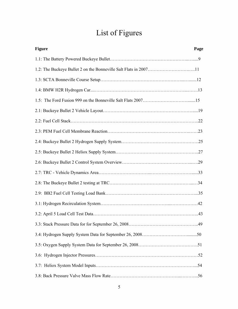
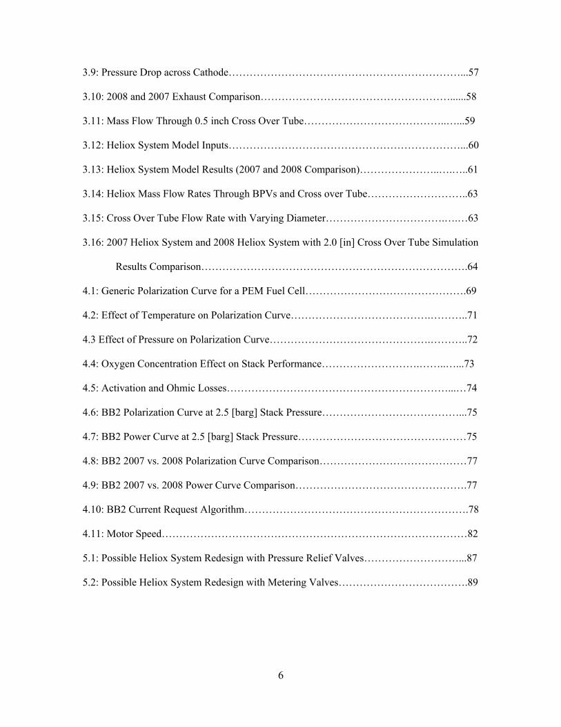
List of Figures
Figure Page
1.1: The Battery Powered Buckeye Bullet……………………………………………..….....9
1.2: The Buckeye Bullet 2 on the Bonneville Salt Flats in 2007……………………….….11
1.3: SCTA Bonneville Course Setup………………………………………………...….......12
1.4: BMW H2R Hydrogen Car....……………………………………………………...…….13
1.5: The Ford Fusion 999 on the Bonneville Salt Flats 2007………………………….......15
2.1: Buckeye Bullet 2 Vehicle Layout…………………………………………………….....19
2.2: Fuel Cell Stack…………………………………………………………………………..22
2.3: PEM Fuel Cell Membrane Reaction……………………………………………….……23
2.4: Buckeye Bullet 2 Hydrogen Supply System…………………………………………….25
2.5: Buckeye Bullet 2 Heliox Supply System………………………………………………..27
2.6: Buckeye Bullet 2 Control System Overview………………………………………...….29
2.7: TRC - Vehicle Dynamics Area……………………………...………………………......33
2.8: The Buckeye Bullet 2 testing at TRC………………………………………………...…34
2.9: BB2 Fuel Cell Testing Load Bank……………………………………………………...35
3.1: Hydrogen Recirculation System………………………………………...………………42
3.2: April 5 Load Cell Test Data……………………………………………………………..43
3.3: Stack Pressure Data for for September 26, 2008………………………………………..49
3.4: Hydrogen Supply System Data for September 26, 2008………………………….........50
3.5: Oxygen Supply System Data for September 26, 2008………………………………….51
3.6: Hydrogen Injector Pressures……………………………………………………………52
3.7: Heliox System Model Inputs…………………………………………………………...54
3.8: Back Pressure Valve Mass Flow Rate………………………………………...………...56
6
3.9: Pressure Drop across Cathode…………………………………………………………...57
3.10: 2008 and 2007 Exhaust Comparison………………………………………………......58
3.11: Mass Flow Through 0.5 inch Cross Over Tube…………………………………..…...59
3.12: Heliox System Model Inputs…………………………………………………………...60
3.13: Heliox System Model Results (2007 and 2008 Comparison)…………………..….…..61
3.14: Heliox Mass Flow Rates Through BPVs and Cross over Tube………………………..63
3.15: Cross Over Tube Flow Rate with Varying Diameter…………………………….….…63
3.16: 2007 Heliox System and 2008 Heliox System with 2.0 [in] Cross Over Tube Simulation
Results Comparison………………………………………………………………….64
4.1: Generic Polarization Curve for a PEM Fuel Cell……………………………………….69
4.2: Effect of Temperature on Polarization Curve………………………………….………..71
4.3 Effect of Pressure on Polarization Curve……………………………………….………..72
4.4: Oxygen Concentration Effect on Stack Performance……………………….……..…...73
4.5: Activation and Ohmic Losses………………………………………………………...…74
4.6: BB2 Polarization Curve at 2.5 [barg] Stack Pressure…………………………………...75
4.7: BB2 Power Curve at 2.5 [barg] Stack Pressure…………………………………………75
4.8: BB2 2007 vs. 2008 Polarization Curve Comparison……………………………………77
4.9: BB2 2007 vs. 2008 Power Curve Comparison………………………………………….77
4.10: BB2 Current Request Algorithm……………………………………………………….78
4.11: Motor Speed……………………………………………………………………………82
5.1: Possible Heliox System Redesign with Pressure Relief Valves………………………...87
5.2: Possible Heliox System Redesign with Metering Valves……………………………….89
7
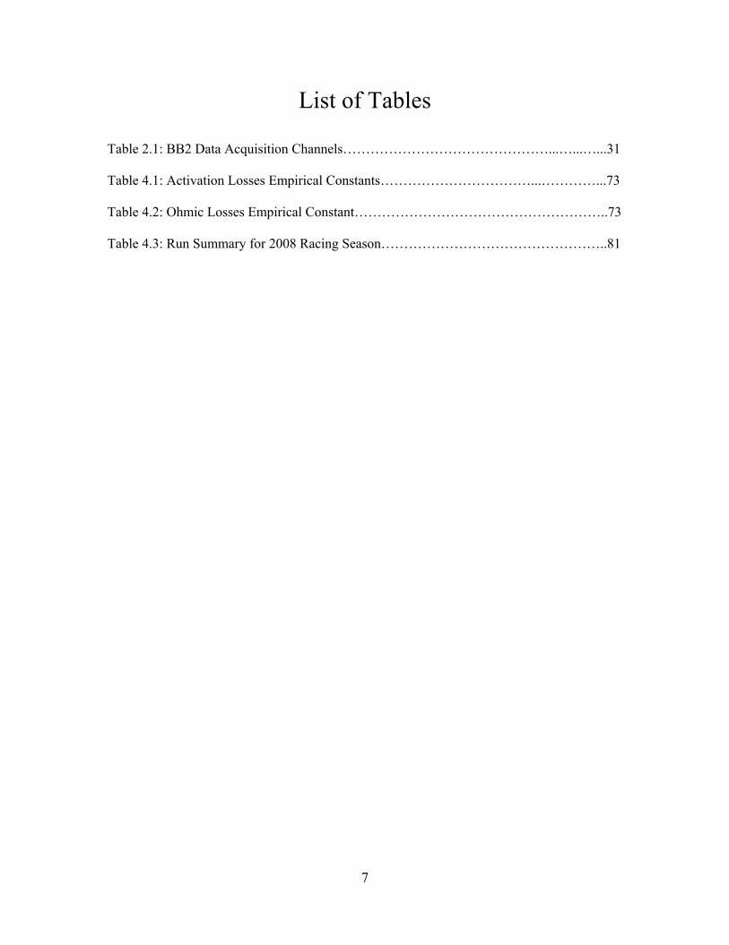
List of Tables
Table 2.1: BB2 Data Acquisition Channels………………………………………...…...…...31
Table 4.1: Activation Losses Empirical Constants……………………………...…………...73
Table 4.2: Ohmic Losses Empirical Constant………………………………………………..73
Table 4.3: Run Summary for 2008 Racing Season…………………………………………..81
8
Chapter 1 :
Introduction to Electric and Hydrogen
Land Speed Racing
This chapter gives information on the history of electric and hydrogen land speed
racing as it directly pertains to this thesis. It discusses the history of land speed racing at
Ohio State as well as previous Hydrogen powered land speed vehicles. It also discusses the
motivation for performing this research and its relevance to today’s automotive community.
1.1 Project Background
Almost immediately after the inception of the first automobiles, man has raced them.
There is an inherent drive to push vehicles to their limits of performance and speed. One of
the purest forms of motorsport is the all-out pursuit of top speed. Know as land speed racing,
this motorsport has been populated by big money teams and backyard mechanics alike. In
the past several years, a team of engineering students from the Ohio State University has
joined the ranks of these speed-enthusiasts as part of the Buckeye Bullet racing program.
1.1.1 The Buckeye Bullet
The Buckeye Bullet program evolved from the Ohio State University Smokin’
Buckeye team which raced in the Formula Lightning racing series during the 1990s. This
series was an intercollegiate series that raced open wheeled battery electric race cars. The

9
series ended in the late 1990s, leaving a group of students with a significant amount of
electric racing experience without a project to work on. This group of students eventually
started what has become the Buckeye Bullet Land Speed Racing Team. The original
Buckeye Bullet (BB1) was a battery powered electric streamliner. A streamliner is a
purpose-built race car for land speed racing. It is characterized by a long narrow body with
enclosed wheels. The Buckeye Bullet is pictured in Figure 1.1. The Buckeye Bullet was
initially powered by 12,000 sub-C cell NiMH batteries. In later seasons the batteries were
upgraded to prismatic NiMH batteries equivalent to that of almost 16 Toyota Prius battery
packs. In August 2004 the BB1 became the first electric car to travel faster than 300 mph.
The BB1 currently holds the record for the fastest electric car both internationally at 438.927
[km/h] (272.737 mph) (under FIA sanctioning) and nationally at 508.485 [km/h]( 315.958
mph )(under SCTA sanctioning).
Figure 1.1: The Battery Powered Buckeye Bullet

10
The Buckeye Bullet last raced in October 2004. At the end of the 2004 racing season
it was determined that the Buckeye Bullet had achieved its top speed potential given the state
of available battery technology at the time. Thus, a new generation of electric land speed
vehicle was proposed.
1.1.2 The Buckeye Bullet 2
What was proposed had never been previously attempted. The next generation, the
Buckeye Bullet 2 (BB2), is the world’s first hydrogen fuel cell powered land speed race car.
Like the BB1, the BB2 was designed and built by students at the Ohio State University with
the help of industry supporters. The most notable of these supports would be Ford Motor
Company and Ballard Power Systems. The Buckeye Bullet 2 is powered two Ballard P5 Fuel
Cell Modules (FCMs). Fuel cells were used in the BB2 as opposed to batteries for several
reasons. Fuel cell systems have been increasing in popularity in recent years and are a strong
candidate for widespread use in transportation applications in the future. Working with fuel
cells offers a whole new set of technical challenges for the Buckeye Bullet team to overcome.
Additionally from a performance standpoint they offer several advantages over batteries in
land speed racing. A batteries voltage and potential power output is dependent on the state of
charge of the battery. During a run the power output decreases as the battery’s state of
charge depletes, meaning that the vehicle can expend less power just when it needs it the
most: at high speed. For a fuel cell system the power output is constant as long there is fuel
available. Therefore, the power output can be constant throughout the entire run.
Additionally a battery takes time to recharge. The BB1 requires several hours of charging for
a complete charge. The BB2 can refueled within approximately 20 minutes. This is
important for international records. In order to obtain an international record the vehicle

11
must make two consecutive runs within an hour. The Buckeye Bullet team is currently
attempting to break the record held by the battery powered BB1 with the fuel cell powered
BB2.
Figure 1.2: The Buckeye Bullet 2 on the Bonneville Salt Flats in 2007
1.1.3 The Bonneville Salt Flats
The mecca for land speed racing is the Bonneville Salt Flats in Utah. The salt flats
are a naturally occurring surface created by an ancient salt lake that has evaporated leaving
behind miles of almost perfectly flat terrain. The salt flats stretch for over 30,000 acres. For
most of the year the salt flats are covered by shallow water, making it not suitable for racing.
However, during the late summer and early fall, the water dries and salt forms a hard surface
ideal for land speed racing.
Before racing events, a strip of salt is compacted and groomed to form a track for
racing. Under the Southern California Timing Association (SCTA) rules, the track consists
of 7 total miles. The first two miles of the track are for acceleration. Miles three through

12
five are timed miles. The last two miles are for deceleration. A timed mile is used to
determine a record. Therefore, the average speed through the fastest time mile is considered
for a record rather than the fastest instantaneous speed. The actual record speed is the
average of two consecutive runs over the same relative or physical mile[1]. Due to the
performance characteristics of the BB2, the fastest mile on a good run is always the fifth
mile. Figure 1.3 shows a depiction of the race course at Bonneville.
Figure 1.3: SCTA Bonneville Course Setup
1.2 Previous Hydrogen Land Speed Records
With many eyes on hydrogen as the world’s answer to green mobility in the future,
several attempts have been made to set land speed records with hydrogen powered vehicles.
1.2.1 The BMW H2R
The BMW H2R set the record for the world’s fastest hydrogen powered car on
September 19, 2004 at the Miramas Proving Grounds in France. The vehicle set nine records
including the fastest flying kilometer for a hydrogen car at 301.95 [km/h] (187.62 [mph]) and
the fastest flying mile at 292.66 [km/h] (181.85 [mph])[2]. Unlike the Buckeye Bullet 2, the
H2R is powered by a 6.0-liter V-12 internal combustion (IC) engine. The engine was based

13
on the BMW 760i’s gasoline powerplant and specially modified to run on hydrogen fuel.
The BMW H2R is shown in Figure 1.4.
The fundamental difference between the H2R and the Buckeye Bullet 2 is that the
H2R’s IC engine burns the hydrogen similar to the way that gasoline is burned in most cars.
The Buckeye Bullet 2 is powered by hydrogen fuel cells. The fuel cells combine hydrogen
and oxygen molecules without combustion and create electric energy directly from the
reaction. This electric energy is then transferred to kinetic energy by an electric motor. This
means that the Buckeye Bullet 2 can develop maximum power with greater efficiency
compared to the H2R.
Figure 1.4: BMW H2R Hydrogen Car [3]

14
1.2.2 The Ford Fusion 999
The Buckeye Bullet 2 was developed with the help of Ford Motor Company. Ford
built the Ford Fusion 999, a hydrogen fuel cell powered land speed car, concurrently with the
Buckeye Bullet 2 project. Both vehicles were a result of the collaboration of the Ford fuel
cell engineers and Ohio State University engineering students. The Ford 999 used the same
motor and inverter as the Buckeye Bullet 2 and a similar fuel cell system. Both the BB2 and
the Ford 999 fuel cell stacks were provided by Ballard Power Systems. The Ford 999 set the
record for the world’s fastest fuel cell vehicle at 333.612 [km/h] (207.297 [mph]) in August
2007 at the Bonneville Salt Flats, Utah [4]. The Ford Fusion 999 is shown in Figure 1.5.
The main difference between the 999 and the BB2 is that the Ford 999 was built to be
a production based race vehicle while the BB2 is a streamliner. The Ford 999 was built on a
Ford Fusion body heavily modified for land speed racing. Aside from the body the vehicle
retained almost no components from the production Ford Fusion. The production body limits
the 999’s potential top speed due to the higher drag coefficient compared to the BB2.

15
Figure 1.5: The Ford Fusion 999 on the Bonneville Salt Flats 2007
1.3 Brief Review of the Buckeye Bullet 2 2007 Racing Season
In August 2007 the Buckeye Bullet 2 made its inaugural appearance on the
Bonneville Salt Flats during Speedweek 2007. In its first appearance on the salt the vehicle
reached a speed of 324.502 [km/h] (201.636 [mph]). In October 2007 the BB2 raced during
the World Finals and during a private FIA sanctioned event. During the World Finals the car
achieved a top speed of 360.977 [km/h] (224.301 [mph]). The BB2 went on to set a world
record for the world’s fastest fuel cell powered vehicle at 212.641 [km/h] (132.129 [mph])
during the FIA meet in October 2007. These speeds attained were fantastic achievements for
the first season of racing. However, the vehicle had serious reliability issues during the 2007
racing season. The car was still far short of its intended goal of breaking 300 mph. Great
advances were made during the 2008 season in terms of reliability, ease of service and
performance. This thesis will document the progression of the BB2 from the 2007 season till

16
the 2008 season and explain the issues encountered, testing approach and methodology
involved in advancing the future of land speed racing even farther.
1.4 Thesis Motivation
The world is in need of new forms of clean, renewable energy both for transportation
and general public usage. This has been demonstrated by numerous publications and billions
of dollars in alternative fuel research. For passenger vehicles a number of manufacturers are
turning to fuel cell technology as a means of replacing the internal combustion engine. These
manufacturers include major names in the industry including: Ford, Daimler, General
Motors, Honda and Nissan. Indeed fuel cell technology holds a lot of potential for the future
of transportation; however, researchers and engineers have many problems to overcome
before fuel cell cars become mainstream. Also, fuel cell technology has many competitors
from battery powered vehicles, to plug-in hybrids and biofuels.
The Buckeye Bullet 2 is a showcase for fuel cell technology. It is meant to show
industry leaders and the general public what a fuel cell powered vehicle is capable of. The
Buckeye Bullet 2 is more than just a student project. Although its main goal remains to
provide experience and learning opportunities for students in Ohio State University’s College
of Engineering, it encompasses more than just education. This project and other alternative
fuel motorsports projects are meant to advance the state of technology for such areas and to
generate excitement about these green technologies. Motorsports inherently has a way of
pushing a technology to the absolute limits of what is possible. Additionally the project is
meant to portray the idea that “green” technology does not necessarily mean slow.
The a main goals of this thesis research are to improve upon the work of previous
team members and address performance and reliability issues encountered by the team during
the 2007 racing season. The main thrust was to perform extensive fuel cell system testing,

17
address shutdown conditions and improve the reliability. Also, it focused on increasing
power output and the accuracy of the fuel cell models. The work done in this thesis will push
the project closer to its goal of breaking 300 [mph] and advancing fuel cell technology while
bringing attention to fuel cells as a viable option for transportation.

18
Chapter 2 :
Vehicle Information and Testing Approach
This chapter gives a brief overview of the major vehicle systems. The focus will be
on the fuel cell and related systems. A brief background on fuel cell basics will be discussed.
The chassis, suspension, braking, body, and parachute systems will not be discussed in depth
in this paper. For further information on these aspects of the BB2 please see that following
references: [5][6][7][8]. Additionally, this chapter explains the testing setup used for fuel
cell system testing for the Buckeye Bullet 2.
2.1 Vehicle Systems Overview
The Buckeye Bullet 2 is far more complex in design and execution when compared to
the original Buckeye Bullet. Unlike the batteries used in the BB1, the fuel cell system in the
BB2 requires the use of a cooling system, gas delivery system, humidification system, and a
more sophisticated control system. This means that very little has been carried over from the
original car. The inverter and motor are the only two main components from the BB1 still
used in the BB2.
2.1.1 Vehicle Layout
In order for the Buckeye Bullet 2 to race, it requires the coordination of multiple
systems to facilitate power generation and direct that power to the wheels. Figure 2.1 shows
the major component layout for the vehicle.
19
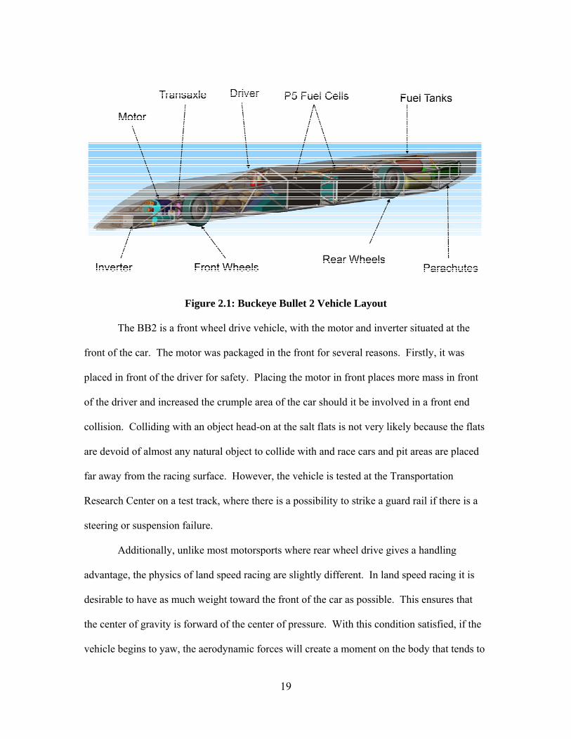
Figure 2.1: Buckeye Bullet 2 Vehicle Layout
The BB2 is a front wheel drive vehicle, with the motor and inverter situated at the
front of the car. The motor was packaged in the front for several reasons. Firstly, it was
placed in front of the driver for safety. Placing the motor in front places more mass in front
of the driver and increased the crumple area of the car should it be involved in a front end
collision. Colliding with an object head-on at the salt flats is not very likely because the flats
are devoid of almost any natural object to collide with and race cars and pit areas are placed
far away from the racing surface. However, the vehicle is tested at the Transportation
Research Center on a test track, where there is a possibility to strike a guard rail if there is a
steering or suspension failure.
Additionally, unlike most motorsports where rear wheel drive gives a handling
advantage, the physics of land speed racing are slightly different. In land speed racing it is
desirable to have as much weight toward the front of the car as possible. This ensures that
the center of gravity is forward of the center of pressure. With this condition satisfied, if the
vehicle begins to yaw, the aerodynamic forces will create a moment on the body that tends to
20
straighten the car. This adds aerodynamic stability to the car at high speeds. Also, since the
racing occurs on salt which can have a coefficient of friction anywhere from .4 to .6
depending on the salt conditions, the rate of acceleration is much less than that of a high
performance car on asphalt. This combined with a wheel base of more than 19 ft means that
there is very little weight transfer under acceleration. The combination of low weight
transfer under acceleration and the fact that the car is designed to have more mass in the front
of the car means that the front wheels will have more traction than the rear wheels. Thus,
having a properly design front wheel car is more advantageous in land speed racing.
The driver is positioned behind the front wheels, this gives him the best visibility and
safety. Additionally, it gives the driver a better sense of how the car is behaving, allowing
him better car control. The driver is protected by a 4130 chromoly steel cage and roll
structure with head restraints. As a redundant safety system the driver is also surrounded by
a carbon fiber honeycomb survival cell. On either side of the driver are the ice tanks which
hold up to 180 [kg] of ice used for cooling the fuel cells. All 180 [kg] of ice will be melting
in a single 90 second run.
The driver section of the car is separated from the rear portion of the vehicle by a
firewall. Directly behind the driver are the two Ballard P5 PEM fuel cell modules. These
modules were originally intended for use in transit city buses; producing up to 125 [kW]
apiece under normal operating conditions. The two modules in use by the BB2 team have
been specially modified for the specific application of land speed racing. These
modifications will be discussed in detail in later chapters.
The fuel cell modules are fueled by the compressed hydrogen and heliox tanks at the
rear of the car behind the rear axle. At the back of the car is the parachute system. The
parachutes are the primary means of deceleration from speeds above 320 [km/h] (~200
[mph]). The vehicle also has a redundant braking system. The vehicle’s mechanical brakes
21
are adapted from Goodrich Aerospace aircraft brakes used on a Lear Jet. These brakes
function similar to a clutch with 2 carbon rotors and 3 carbon stators. Many conventional
high performance automotive brake packages were considered for the vehicle, however, none
of them were capable of stopping the vehicle from top speed. The Goodrich brakes have the
capacity to stop the car from 500+ [km/h]. These brakes can be used for low speeds like
regular automotive brakes. Although they can stop the car from 500 [km/h], performing this
action will destroy the brakes. So they can only perform a high speed stop once. This is
perfectly acceptable because the brakes are only a backup system in case the parachute
system fails.
2.1.2 Fuel Cell System Introduction
A fuel cell is an electrochemical device that combines a fuel and an oxidant without
combustion and creates electricity directly. The Ballard P5 fuel cells used for the BB2, as
with many fuel cell systems, use hydrogen as the fuel and oxygen as the oxidant. The most
typical kind of fuel cell used in automotive applications is the permeable electron membrane
(PEM) fuel cells. PEM fuel cells work at low temperatures compared to other types of fuel
cells which means that they can be started quickly. This is a strong advantage for the vehicle
applications as customers are accustomed to internal combustion engines which require very
short startup time. Also PEM membranes can be made very thin which allows the total stack
to be more compact. Another advantage PEM fuel cells have for vehicle applications is that
they do not contain any corrosive fluid that other types of fuel cells contain. [9]
The PEM fuel cell consists of membrane electrode assemblies (MEAs) sandwiched
between bipolar plates. Multiple bipolar plates and MEAs are connected together to form the
fuel cell stack. Each cell produces between 1.2 and .5 volts depending on its loading
condition. The cells in the stack are connected in series which allows the overall stack in the

22
case of the BB2 to operate between 960 to 550 [V]. Figure 2.2 shows a generic exploded
diagram of a fuel cell stack with multiple MEAs and bipolar plates.
Figure 2.2: Fuel Cell Stack [10]
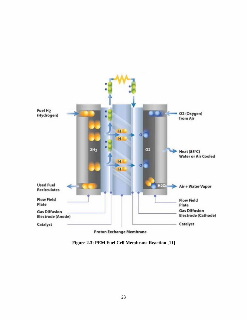
The MEA consists of an electrolytic polymer with catalyzed electrodes bonded to
either side. The electrolyte polymer allows the transfer of H+ ions across the membrane.
During operation, hydrogen is supplied on the anode side of the membrane and oxygen is
supplied on the cathode. The hydrogen atom ionizes to form H+ ions on the catalyzed anode
side of the membrane. The H+ ion then passes through the polymer membrane while the
electron travels through the bipolar plates and recombines with hydrogen and oxygen on
cathode to produce water. It is this flow of electrons that create the electric power that the
fuel cell outputs. The only products from the reaction are water, electricity and heat. Figure
2.3 shows a diagram of a typical PEM fuel cell reaction.
23
Figure 2.3: PEM Fuel Cell Membrane Reaction [11]

24
2.1.3 Gas Delivery System
The gaseous hydrogen that powers the fuel cells is stored at 350 [bar] in a DOT
approved carbon fiber and aluminum tank. A schematic of the hydrogen delivery system is
displayed in Figure 2.4. The hydrogen is stepped down from 350 [bar] to 17 [bar] by two
first stage regulators plumbed in parallel. The hydrogen is further reduced in pressure inside
each FCM by the hydrogen low pressure regulator. This regulator determines the pressure
that is delivered to the hydrogen injectors. During idle and low current draw the pressure
upstream of the injectors is approximately the same as the hydrogen loop stack pressure.
Under full current draw however this pressure can increase up to the hydrogen supply
pressure. Two injector nozzles are used in each stack. One nozzle is sized to supply
hydrogen at idle and low current draw. The larger nozzle is used to supply hydrogen during
high current draw. The original P5 module switched between the high and low flow injectors
depending on the current draw. This function has been disabled on the BB2 modules for
reasons discussed in chapter 3.

25

26
Most vehicle fuel cell systems use ambient air for the oxidant in the cathode loop of
the fuel cell. Like most pressurized fuel cell systems, the standard P5 module was designed
to use a motor driven compressor to compress ambient air to stack pressure. The BB2 uses
compressed heliox stored onboard in tanks rather than using a compressor. Using
compressed heliox rather than air has several advantages. First, the vehicle does not need to
carry on onboard compressor, which uses a significant portion of the energy generated by the
fuel cell. A compressor can use as much as 20% of the power produced by the fuel cell
stack. For the BB2 this would mean that 120 [kW] would be used to drive a compressor
rather than driving the vehicle forward. Additionally, the vehicle is raced on the Bonneville
Salt Flats. Any air drawn into the vehicle would contain salt particles as well as other
contaminants and would thus need to be filtered. Inevitably some contaminants would enter
the gas system and the stack and could reduce performance over time. Also, arguably the
most important reason the BB2 runs on compressed oxidant is because it allows the use of
higher concentrations of oxygen than ambient air. The vehicle currently uses a mixture of
60% helium and 40% oxygen. The higher oxygen concentration increases the power output
of the modules. This is discussed in more detail in the following chapters. Helium was used
rather than nitrogen as a mixing gas because it allowed for a lower mass flow rate of gas for
the same molar flow rate of oxygen. A lower mass flow rate results in lower pressure drops
across gas system restrictions and allows for the use of smaller pressure regulators.
Performance could be increased by using even higher oxygen concentration, how 100%
oxygen is very dangerous under high pressure. 40% oxygen was determined to be a good
compromise between increased performance and safety. Figure 2.5 shows a schematic of the
the BB2’s heliox delivery system.
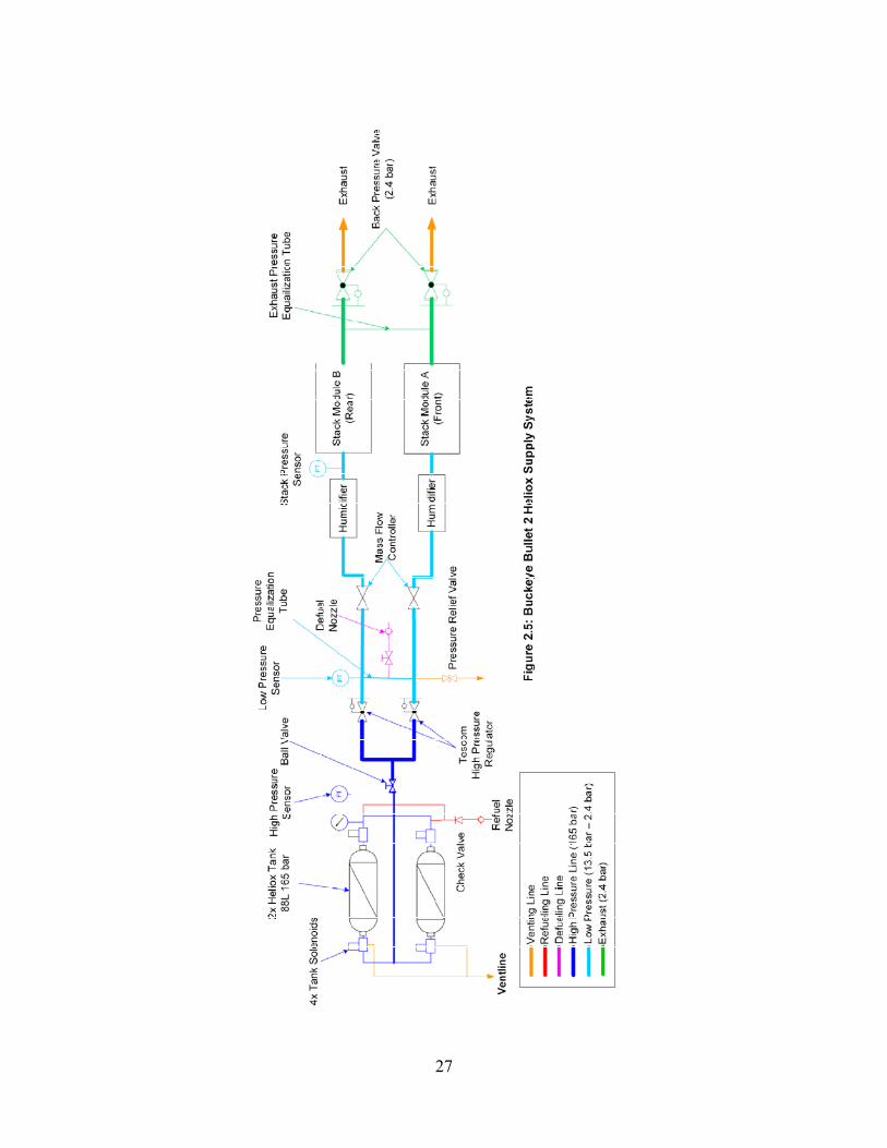
27

28
2.1.4 Cooling System
Fuel cell systems are generally more efficient than internal combustion engines [9],
however, they are still not perfect. The BB2 fuel cell system is approximately 50% efficient.
This means that if it is producing 500 [kW] of electricity it is also creating about 500 [kW] of
heat energy that needs to be removed from the system to ensure that it does not overheat.
The fuel cell system on the BB2 is design to operate at 80o C ideally. If the fuel cells reach
much higher than that temperature this could damage the MEAs and reduce the power output
of the stacks. The vehicle uses an ice bath to cool the modules. Ice was used as a heat sink
because it has the ability to absorb large amounts of energy by utilizing the phase change
from solid to liquid water. The vehicle uses 180 [kg] of ice each run. Therefore, it is
important that ice is cheap and easy to obtain. The cooling system uses two isolated loops for
cooling. The water flowing through the stack is isolated from the water flowing through the
ice tanks. This is because the water flowing through the stack is in contact with the bipolar
plates and thus must be deionized to avoid conducting electricity. Heat from the fuel cell
water loop is transferred to the ice tank loop through two heat exchangers mounted on either
side of the forward fuel cell module. Using two isolated loops allows the water in the ice
side to be relatively “dirty”, meaning that any source of ice can be used in the ice tanks.
2.1.5 Electric Motor
The BB2 uses the same motor and inverter as the original Buckeye Bullet. The motor
is a three phase AC induction motor and was custom made for the Buckeye Bullet program.
It is specially designed for land speed racing. It is able to deliver a large amount of power
over a short duration. The motor is capable of running at 520 [kW] for approximately 2
minutes. It can perform two runs like this within an hour of each other.

29
2.1.6 Control System
The BB2 uses sophisticated multilevel control system. Figure 2.6 shows an overview
of the BB2 control system. The Motohawk controller is the top level controller that controls
and coordinates between the other control devices. The Motohawk receives input from the
driver and the sends the appropriate commands to the inverter and Ballard controller. It also
monitors select data channels and relays information to the driver via the Bosch display. The
driver is able to see information such as speed, motor rpm, gear selection, as well as vehicle
warnings such as low hydrogen or heliox pressure. The same controller and software used in
the Ballard Bus Program has been retained for use in the BB2. This controller controls all
fuel cell functions and control. The original software from the Ballard Buses has been
specially modified for the use of the BB2.
Figure 2.6: Buckeye Bullet 2 Control System Overview

30
2.1.7 Data Acquisition System
Data collection is very important for prototype vehicles like the BB2. Without the
proper data available it is impossible to properly assess vehicle issues and failures. Data is
collected for each test and run of the vehicle. The vehicle has two data collection systems.
The Ballard data logger from the Ballard Buses is used to monitor data channels from inside
the fuel cell module such as stack pressure, temperature, control valve positions, heliox mass
flow rates, voltage, current, hydrogen leak detectors, smoke detectors etc. The voltage of
each cell row is also measure using the cell voltage monitors (CVMs). The individual cell
voltages are recorded using the Ballard data logger. The CVM measurements are very
important in diagnosing system issues. Low cells and reversed cell are symptoms of oxidant
or fuel starvation at the stack or flooding inside the module. Low cells are discussed further
in chapter 3. The National Instrument Compact Rio also functions as a data logger for the
other vehicle systems. This device records motor rpm, speed, cooling system temperatures,
gas supply pressures, etc. A more in depth list of Compact Rio data channels is shown in
Table 2.1. This list is not comprehensive.

31
Catergory SensorCockpit Throttle Pedal Input Cockpit 24V Battery Voltage Cockpit 12V Battery Voltage Cockpit Clutch Limit Switch Cockpit Clutch Pressure Cockpit Front Break Pressure Cockpit Rear Break Pressure Cockpit Brake Power Assist Accumulator Pressure Cockpit Control System Active LED Cockpit Up Shift Signal Cockpit Down Shift Signal Driveline Motor Speed Driveline Motor Temperature Driveline Transmission Temperature Driveline Transmission Gear Driveline Torque Reference to Inverter Driveline Inverter High Voltage Cooling 48V Battery Voltage Cooling Fuel Cell Cooling Loop Pump Command Cooling Ice Bath Cooling Loop Pump Command Cooling Coolant Pressure Module A Cooling Coolant Pressure Module B Heliox System Heliox Tank Pressure Heliox System Heliox Low Pressure Heliox System Heliox Pressure Before MFC Heliox System Heliox Pressure at Stack Inlet FCM A Heliox System Heliox Pressure at Stack Inlet FCM B Hydrogen System Hydrogen Tank Temperature Hydrogen System Hydrogen Tank Pressure Hydrogen System Hydrogen Low Pressure upstream Hydrogen System Hydrogen Low Pressure downstream Hydrogen System Hydrogen Pressure Before Injector FCM A Hydrogen System Hydrogen Pressure Before Injector FCM B Hydrogen System Hydrogen Pressure at Stack Inlet FCM A Hydrogen System Hydrogen Pressure at Stack Inlet FCM A Hydrogen System Hydrogen Pressure at Stack Outlet FCM A Hydrogen System Hydrogen Pressure at Stack Outlet FCM B Fuel Cell FCM B Voltage Fuel Cell FCM A Voltage GPS System GPS Speed GPS System GPS Heading
Table 2.1: BB2 Data Acquisition Channels
32
2.2 Fuel Cell System Test Setup
It was clear after the 2007 racing season that one of the largest issues facing the BB2
team was the need for better and easier procedures for testing the fuel cell systems. Prior to
the 2007 racing season there were only two main methods generally available to the Buckeye
Bullet team members for load testing the fuel cell systems. These methods were
dynamometer testing and track testing. Both of these test methods have advantages and
disadvantages for testing the fuel cell systems. However, both of them require extensive
setup time and effort.
2.2.1 Dynamometer Testing
A dynamometer is a machine that measures torque and speed of a motor and absorbs
the power output of the motor. The Center for Automotive Research at the Ohio State
University has two 745 [kW] (1000 [hp]) dynamometers that are available for BB2 team use.
During dynamometer testing it is required to remove the motor from the vehicle to connect it
to the dynamometer. During dynamometer testing, electric power it generated by the fuel
cells and sent through the inverter and into the motor. The motor transfers the electric power
into mechanical energy which is absorbed by the dynamometer.
This method of testing is useful for testing the overall driveline system and testing
how the motor, inverter and fuel cell systems work together. However, it takes two team
members working for an entire day to remove the motor from the car and setup the vehicle
for dynamometer testing as well as another day to do the reverse operation. For most of the
testing performed in 2008 the team was only interested in testing the fuel cell system. The
inverter and motor add additional variables to the test setup. Additionally, dynamometer
testing results in additional wear to the motor. Again, the motor is custom built and not
easily replaceable.

33
2.2.2 TRC Testing
The vehicle is track tested at the Transportation Research Center (TRC) in East
Liberty, Ohio. This is the only place other than the salt flats where the BB2 can run under its
own power. TRC has many testing areas including a dynamic handing course, gravel road,
durability testing areas and a 7 mile outer oval course. The BB2 tests on the Vechile
Dynamics Area (VDA) which consists of a large ~2 mile figure-8 circuit. An aerial view of
the VDA is shown in Figure 2.7.
Figure 2.7: TRC - Vehicle Dynamics Area
TRC testing is excellent for testing the entire vehicle. It not only tests the fuel cell
systems but also the transmission, suspension, brakes and parachute system. However, track
testing is less desirable if one only wants to test the fuel cell system. During TRC testing the
vehicle is able to test up to 160 [km/h]. Although this sounds fast for any vehicle, the BB2
does not even leave first gear at this speed. In fact, most of the testing performed at TRC is
not at full power because the vehicle spends most of the time at lower speeds where the
motor is not yet into its peak power region. Therefore, the fuel cell system cannot be
adequately tested at full power at TRC. Also, getting the car to the track and preparing it for
testing requires the effort of many team members and requires packing the car and support

34
equipment and transporting it to TRC. A picture of the BB2 testing at TRC is shown in
Figure 2.8.
Figure 2.8: The Buckeye Bullet 2 testing at TRC
2.2.3 Load Bank Testing
In response to the issues with the current testing methods a new fuel cell testing
method was necessary. A load bank was constructed to convert the electrical energy
produced by the fuel cells into heat energy that is then dissipated into the atmosphere. The
load bank consists of nine Avtron resistors ranging from 7.80 Ω to 5.10 Ω. The resistors can
be switched on individually, allowing the fuel cells to be run at nine discrete power levels
from low power up to full power. A picture of the load bank is displayed in Figure 2.9.
The resistors are cooled by a 11 [kW] three phase electric fan. When used with the
fan, the load bank is able to dissipate the 600+ [kW] that the two fuel cells combined can
generate for the 90 second duty cycle over which the car will typically run. Additional the
load bank can be used for short duration testing (<10 seconds) without cooling. This is
useful because it makes it possible to test the fuel cell on the salt flats without running the

35
car. Therefore, short tests can be performed in the pits without wasting valuable time on the
salt flats. One of the greatest advantages of the load bank is that it allows the fuel cell system
to be tested regardless of the condition of the rest of the vehicle. This means that the fuel
cells can be tested if the rest of the vehicle is disassembled or if the vehicle has just been run
on the salt. It takes less than 5 minutes to transition from a track ready car to the load bank
configuration. To transition to fuel cell testing the high voltage cables only need to be
removed from the inverter and plugged into the load bank. This saves valuable time during
testing and allows fuel cell system issues to be addressed quickly and separately from other
vehicle systems.
Figure 2.9: BB2 Fuel Cell Testing Load Bank
36
Chapter 3 :
Vehicle Design Improvements and Modifications
Land speed racing requires very unique design considerations for vehicles compared
to road cars and even other types of motorsports. This means that the requirements for the
fuel cells used for the Buckeye Bullet 2 are very different from those for which they were
originally designed. The Ballard P5 fuel cell modules were originally designed for city
transit buses that run at moderate power levels for an extended period of type with varying
power output. The BB2 runs for very short durations, usually under 90 seconds, and at full
power output for close to 85% of its run time. Therefore, the P5 fuel cell modules underwent
several modifications to optimize their design for land speed racing. This chapter will give a
brief review of the BB2’s first racing season in 2007 and highlight the changes that were
made to the fuel cell systems before the 2008 season. This chapter also contains analysis of
the over pressure events that occurred during the 2008 season.
3.1 Review of 2007 Racing Season
The BB2 was first raced on the Bonneville Salt Flats during Speed Week 2007. The
BB2’s highest recorded speed during that week was 324.502 [km/h] (201.636 [mph]). The
car reached a speed of 360.977 [km/h] (224.301 [mph]) during World Finals in October
2007. This became the fastest ever recorded speed for a hydrogen vehicle beating the Ford
999’s top recorded speed of 333.612 [km/h]. It should be noted that these are not

37
considered records under the SCTA because both the BB2 and the Fusion 999 are
categorized at straight electric vehicles in the E3 class. Therefore, the speed they would
need to break to be considered for a recorded is the all out electric land speed record set
by the original Buckeye Bullet at 508.485 [km/h]. The BB2 went on to set a FIA
sanctioned world record for the world’s fastest fuel cell vehicle at 212.641 [km/h]
(132.129 [mph]) during a private FIA meet following World Finals in 2007. All of the
speeds attained during the 2007 racing were fantastic results that pushed the envelope of
fuel cell technology. However, all the attempts fell short of the vehicle’s original design
goals to break 300 [mph] and contend with the BB1’s record for the world’s fastest
electric car.
There were many issues that plagued the 2007 racing season for the BB2. Keep
in mind that this was the first year the vehicle had ever been track tested or raced. It took
the original Buckeye Bullet three years of racing before it set the mark at the current
record. The BB1 also set its record using batteries rather than fuel cells. Although
batteries contain their own issues and pitfalls, the fuel cell system is massively more
complex than the battery packs. This can be easily illustrated by looking at the amount of
data being record by the two vehicles. The BB1 originally only recorded 4 data channels:
vehicle speed, motor rpm, voltage and current. The BB2 monitors hundreds of data
channels from voltage and current to gas system pressures, cooling temperatures,
solenoid positions, hydrogen sensors, etc.
Given the enormous amount of complexity, the team was still able to set a world
record during that first racing season. However, several issues still needed to be
38
addressed before the following racing season in order to achieve the program goals. A
new primary goal was set for the 2008 season: develop a reliable fuel cell system.
Most aborted runs during the 2007 season were a result of an automatic vehicle
shutdown. The Ballard controller monitors a variety of data channels and will shutdown
the fuel cell system when a number of conditions are met. These shutdowns are triggered
to prevent damage to fuel cell components and to ensure safety. The shutdowns during
the 2007 season were most commonly caused by detection of hydrogen leaks and low cell
voltages.
As part of the safety strategy, the Ballard controller monitors the hydrogen
concentration inside each module. A hydrogen sensor is placed in front of an exhaust fan
on the outer casing of each module. A vent on the front of each module allows ambient
air to be drawn into the module. This reduces the chances that a small hydrogen leak can
lead to a buildup of hydrogen in the module and result in a hydrogen concentration above
the flammable limit. All the air in the module that is drawn out by the exhaust fan passes
over the hydrogen detector. Hydrogen is flammable at 4% in air. The Ballard controller
will shut down both modules and close the hydrogen tank solenoid if the hydrogen sensor
registers a reading of 50% of the lower flammability limit for hydrogen (2% hydrogen
concentration) for longer than ~2-3 seconds. Several run attempts during the 2007 racing
season were aborted due to hydrogen leaks. The reaction to these hydrogen leaks is
discussed later in this chapter.
Another common shutdown condition for the vehicle in 2007 was low or reversed
cell voltages. Each voltage of the total 1920 individual cells in the BB2 is monitored and
recorded during the run. If any cell reads below .2 [V] for a short period (~5 seconds) the

39
modules will shutdown. These low cells are caused by a number of problems. Low cells
can be caused by low oxygen or hydrogen concentration on the cathode and anode,
respectively. The low reactant concentration can be attributed to restrictions in the
supply system, improper regulator settings resulting in low reactant pressure and reactant
leaks. Also, a low cell can be caused by water flooding. If the pores on an electrode or
the gas diffusion layer flood this will block the reactants from reaching the catalyst sites.
Product water is removed from the stack by the flow of reactant through the stack. If the
reactant velocity is not high to remove the product water adequately, reactant starvation
will occur. The rate at which water produced in the fuel cell is directly proportional to
current. Although water is not produced on the anode, water removal from the anode is
still a concern. Product water will travel through the membrane and collect on the anode;
therefore, flooding can occur there. A reversed cell is one that actually measures a
negative voltage. A reversed cell is caused by a low concentration of hydrogen.
These low and reversed cell essentially become resistors in the stack. They
reduce the overall stack power output. They also generate heat and if not addressed can
cause serious damage. The heat generated in combination with a catalyst can cause
hydrogen ignition if there is an internal stack leak that allows the correct concentration of
oxygen and hydrogen to occur. Also, the low and reversed cell can cause permanent
damage to the membranes which can affect their power output even after the cell returns
to normal operating voltage.
The largest issue facing the team at the end of the 2007 season was low and
reversed cells. The most significant reason for these low cells was hydrogen starvation in

40
the anode loop. The diagnosis and reaction to these failures is discussed in detail in the
following sections.
3.2 Hydrogen Leaks and Detection
Hydrogen has the lowest molecular weight and viscosity of any gas, therefore, it
has the highest leak rate compared to other gases and is more difficult to contain [12]. It
is very expensive and difficult to make a hydrogen system that is completely sealed. The
greatest leak potential is not within the stainless steel fittings that supply the fuel cells but
rather in the stacks themselves. There is always an accepted leak rate when dealing with
hydrogen systems. The BB2’s specification for acceptable leak rate at operating pressure
for one module is 2.5 [slpm] of hydrogen.
The air within each module is evacuated continuously with an exhaust fan on each
module. This reduces that chances that hydrogen will build up within the module and
reach a potentially flammable limit.
There are several methods that the BB2 uses to check for leaks in the hydrogen
system. The most extensive method is to connect the module to a leak checking device.
The leak check device allows the system to be pressurized and then measures the flow
rate of gases flowing through the device. This effectively quantifies the leak rate. The
coolant, heliox and hydrogen leak rates can be measured individually. Additionally the
cross leak rates between anode and cathode and coolant can be measured. This tool not
only measures the line leaks within the module but also the leak rates within the stack.
Another form of leak check that is less extensive and easily performed involves
pressurizing the system by opening the fuel tank and closing the purge valve. Then each
41
fitting needs to be either sprayed with soapy solution that indicates leaks by bubbling or a
hydrogen detector can be used to check each fitting for leaks.
In order to reduce the vehicle shutdowns due to hydrogen leak detections, the
Buckeye Bullet team adopted a more rigorous leak checking schedule. Under normal
operation the fuel cell modules would be leak checked after several hundred hours of
operation. During the 2008 racing season, each BB2 module was subjected to a full
metered leak check using a leak check device before each trip and then leak checked on
the salt using a hydrogen detector. This significantly reduced the hydrogen leaks
detected during operation.
3.3 Module Hardware Changes
The two fuel cell modules used for the BB2 are specially modified for the unique
characteristics of land speed racing. The BB2 modules run at a much higher power level than
the original P5 specification and thus the hydrogen system needed to be changed to account
for the increased hydrogen flow. Also, some systems were able to be removed to reduce
overall vehicle weight.
3.3.1 Hydrogen Injector Assembly
The amount of hydrogen consumed on the anode is directly proportional to the
current draw. If the hydrogen supply system to the stack is not able to flow enough
hydrogen, the concentration of hydrogen in the stack will decrease leading to hydrogen
starvation on the stack. Hydrogen starvation results in low cell voltages as previously
discussed. Additionally, even if the proper concentration of hydrogen is maintained on the
stack, if the hydrogen flow rate is not high enough flooding in the anode can occur.
For these reasons the hydrogen is circulated through the stack to ensure that there is
adequate flow velocity to remove product water. To facilitate this action some fuel cell

42
systems use an electric pump to recirculate the hydrogen. The P5 module uses a jet pump to
recirculate hydrogen. The flow of the hydrogen through the stack is driven by a combination
of hydrogen being consumed in the reaction and the momentum of the pressurized hydrogen
entering the anode loop through an orifice. A diagram of this system is shown in Figure 3.1.
Figure 3.1: Hydrogen Recirculation System
The hydrogen flow rate through the injector orifice is dependent on the orifice sizing
and the hydrogen inlet pressure. Each module contains one low flow and one high flow
injector for low current and high current, respectively. The normal P5 module will switch on
the high flow injector for high current draw. The low flow injector is always open.
The main issue during early testing in Spring 2008 was global hydrogen starvation in
both fuel cell modules. From Figure 3.1 it can be seen that hydrogen pressure in both stacks
drops off quickly at current draws greater than 600 combined amps. The supply pressure to
the injector assembly droops to ~ 9 [bar] during this high current area.

43
Figure 3.2: April 5 Load Cell Test Data
10 20 30 40 50 60 70 80 900
0.5
1
1.5
2
time [s]
Pres
sure
[bar
]
Heliox PressureH2 Stack Pressure Mod AH2 Stack Pressure Mod B
10 20 30 40 50 60 70 80 900
100
200
300
400
time [s]
Curr
ent [
Amps
]
Mod A CurrentMod B Current
10 20 30 40 50 60 70 80 900
2
4
6
8
10
12
time [s]
Pres
sure
[bar
]
Hydrogen Supply Pressure

44
Over several tests the supply pressure was increased to ~14.1 [bar] at fuel cell module
inlet. This increased the maximum possible current draw with some success, however,
hydrogen starvation continued to be a problem. Further increase of the hydrogen pressure
was not possible due to the rated pressure of certain hydrogen system components.
The mass flow rate needed is directly proportional to the current draw. The desired
mass flow rate of hydrogen can be determined by calculating the hydrogen consumed in the
fuel cell reaction:
2
where =desired mass flow rate of hydrogen ([g/s])
I = Current draw [A] F=Faraday’s Constant (96485 [C/mol]) MH2= Molecular mass of hydrogen (2.016 [g/mol]) Ncells= 960
500
2 964852.016 960
5.015 ⁄
The idle jet is able to deliver approximately 0.4 [g/s] of hydrogen under the described
loading condition. Therefore, the high flow injector needs to deliver 4.615 [g/s]. It should be
noted that normally more hydrogen is injected into that stack than is consumed for the
reaction. The excess hydrogen is purged during the normal purge cycling and also leaks
through the stack into the cathode loop. The hydrogen that leaks into the cathode loop is
carried out with the exhaust. The hydrogen that is purged exits the vehicle through the
exhaust. The purge valve periodically opens to remove helium and oxygen contaminants that
leak over from the cathode and lower hydrogen concentration on the anode. The contaminant
buildup in the anode is very minimal in 90 seconds. Therefore, the purge valve is always

45
closed above 300 [A] per module. Eliminating the purge cycle at high current draw helps to
maintain hydrogen pressure. Because no hydrogen is purged during high current draw and
very little leaks across the stack, the excess hydrogen entering the stack will be ignored for
the following calculations.
The actual mass flow rate of the hydrogen entering the stack through the high flow
injector is determined by the isentropic choked flow through a nozzle equation [13]:
21
where
po = absolute pressure before the injector [Pa] A* = area of the orifice [m^2] R = Ideal Gas Constant for Hydrogen (4124 [J/(kg*K)]) To = temperature before the injector [K] γ = specific heat ratio for hydrogen (1.41)
During the 2007 racing season the high flow injector orifice was 2.74 [mm] in
diameter. For the high flow injector with an orifice size of 2.74 [mm] at 10 [barg] before the
injector (note that 10 [barg] would correspond with 14.1 [barg] at the module inlet), the mass
flow rate is calculated as follows:
9.976 10 5.896 101.41
4124 273
.
.
3.804 [g/s]
This value shows that the mass flow rate through the choked flow injector is not
sufficient to supply the reaction at high current. Therefore, fuel starvation in the stack was
caused by the orifice of the injector being sized to small.
46
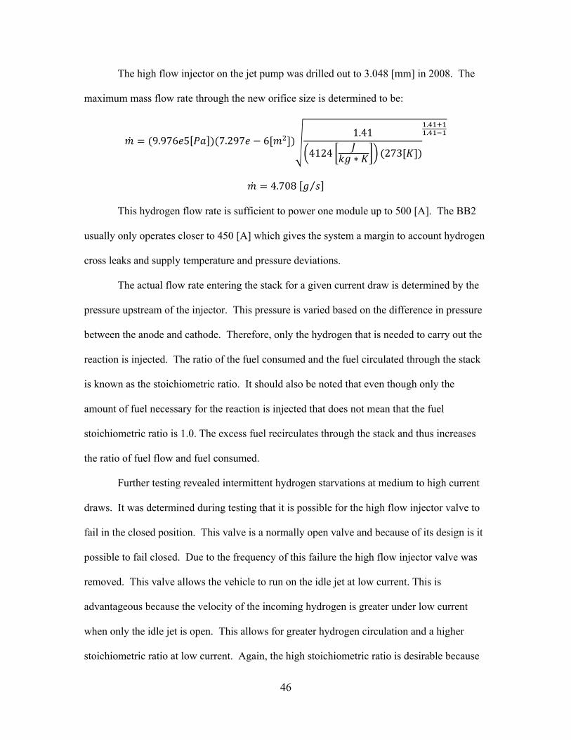
The high flow injector on the jet pump was drilled out to 3.048 [mm] in 2008. The
maximum mass flow rate through the new orifice size is determined to be:
9.976 5 7.297 61.41
4124 273
.
.
4.708 ⁄
This hydrogen flow rate is sufficient to power one module up to 500 [A]. The BB2
usually only operates closer to 450 [A] which gives the system a margin to account hydrogen
cross leaks and supply temperature and pressure deviations.
The actual flow rate entering the stack for a given current draw is determined by the
pressure upstream of the injector. This pressure is varied based on the difference in pressure
between the anode and cathode. Therefore, only the hydrogen that is needed to carry out the
reaction is injected. The ratio of the fuel consumed and the fuel circulated through the stack
is known as the stoichiometric ratio. It should also be noted that even though only the
amount of fuel necessary for the reaction is injected that does not mean that the fuel
stoichiometric ratio is 1.0. The excess fuel recirculates through the stack and thus increases
the ratio of fuel flow and fuel consumed.
Further testing revealed intermittent hydrogen starvations at medium to high current
draws. It was determined during testing that it is possible for the high flow injector valve to
fail in the closed position. This valve is a normally open valve and because of its design is it
possible to fail closed. Due to the frequency of this failure the high flow injector valve was
removed. This valve allows the vehicle to run on the idle jet at low current. This is
advantageous because the velocity of the incoming hydrogen is greater under low current
when only the idle jet is open. This allows for greater hydrogen circulation and a higher
stoichiometric ratio at low current. Again, the high stoichiometric ratio is desirable because

47
it helps remove water from the anode and ensures high hydrogen pressure and concentration
downstream in the stack. However, because the BB2 only operates at low power for a very
short amount of time, the valve was removed so that the BB2 always runs with both injectors
open.
3.3.2 Weight Reduction
Weight is the enemy of any high performance vehicle. Weight is not directly related
to the top speed of a vehicle. The absolute top speed occurs when the force pushing the car
forward by the drivetrain and the wheels equals the aerodynamic and rolling resistance forces
pushing the vehicle backwards. Therefore, top speed is directly a function of engine power,
traction, rolling resistance and aerodynamic resistance. However, the BB2 is accelerating
even through the last timed mile. Therefore, any weight reduction and subsequent increase in
acceleration results in a higher exit speed in the final timed mile. So reducing weight results
in a higher recorded speed. In the 2007 racing season the BB2 weighed approximately 2700
[kg] with a driver and loaded with cooling ice. Throughout 2008 many improvement were
made to the BB2 to reduce weight where possible. The cooling system and gas delivery
systems were revised to utilize light weight materials and reduce complexity.
Additionally, unnecessary systems were removed from the fuel cell modules in order
to reduce weight. The aluminum covers for the fuel cell panel were replaced with carbon
fiber panels or thinner walled aluminum panels. Also, the exhaust water recapture system
was removed. Normally the product water from the fuel cell stack is removed from the
exhaust and used in the humidification system. This eliminates the need to refill the
humidification system with water during the bus operation. However, for the BB2
application it is lighter to actually store more water on board and remove the water recapture
system.

48
All the weight reduction projects resulted in approximately 220 [kg] of weight being
removed from the vehicle.
3.4 Overpressure Event Analysis
During Speedweek 2008 the fuel cell system showed remarkable improvement in
reliability compared to the previous season. Throughout the first four days of racing there
were no aborted runs due to fuel cell issues. On August 23, 2008 after two aborted runs due
to a failure of the humidification pump on module B, the third run of the day resulted in
shutdown due to a hydrogen leak detection. After pulling the vehicle back into the pit area
and investigating further, it was discovered that a stack seal had be damaged by a pressure
spike in both the anode and cathode loop in module B. The pressure spike was attributed to a
malfunction of the mass flow controller (MFC) for module B. After bench testing MFC B
after the event, it was concluded that the MFC had failed due to an electrical failure caused
by corrosion and water intrusion on the MFC’s circuitry. At the time, the MFC for module A
did not exhibit this problem behavior. MFC B was subsequently replaced with a new MFC
of the same model.
During the FIA meet on September 26, 2008, the vehicle experienced a similar over
pressure event resulting in a blown seal in the fuel cell stack. The escaping hydrogen
and heliox ignited due to an unknown source and caused minor damage to the
vehicle. The majority of the damage occurred to the vehicle’s body panels and the
fuel cell module panels. All the major vehicle systems and more importantly the
driver survived the event without any harm.
3.4.1 Overpressure Event Data
Data from both over pressure events are very similar, thus we will focus on the more
severe over pressure event during the FIA meet. Figure 3.3 shows the stack pressures during

49
the overpressure event during the FIA meet in September 2008. From the data it can be seen
that the anode and cathode pressure spike in both modules just prior to hydrogen leak
detection. It should be noted that the pressure sensors used at the stack level saturate at 3.2
[bar]. Therefore, during the pressure spike, it is unclear of the actual pressure on the stack. It
is only known that the pressure is equal to or greater than 3.2 [bar]
Figure 3.3: Stack Pressure Data for for September 26, 2008
Figures 3.4 and 3.5 show the pressure data taken from the September 26 run for the
hydrogen and oxygen systems respectively. Figure 3.4 also shows the hydrogen detection
sensor reading. Figure 3.5 also shows the mass flow rate through the mass flow controllers.
0 5 10 15 20 25 30 35 40 45 50 550
0.5
1
1.5
2
2.5
3
3.5
Time [s]
Pre
ssur
e [b
arg]
Anode and Cathode Pressures
O2 Pressure Module A
O2 Pressure Module B
H2 Pressure Module A
H2 Pressure Module B
OPE
Pressure Spike

50
Figure 3.4: Hydrogen Supply System Data for September 26, 2008
0 10 20 30 40 50 600
100
200
300
400Pr
essu
re [b
arg]
Hydrogen Supply System
H2 Tank Pressure
OPE
0 10 20 30 40 50 600
5
10
15
20
Pres
sure
[bar
g]
H2 Pressure Before Low Pressure Regulator
OPE
0 10 20 30 40 50 600
1
2
3
4
Pres
sure
[Bar
g]
H2 Stack Pressure A
H2 Stack Pressure B
OPE
0 10 20 30 40 50 600
20
40
60
Time [s]
Leak
Det
ecto
r [%
LFL]
H2 Leak A
H2 Leak B
OPE

51
Figure 3.5: Oxygen Supply System Data for September 26, 2008
0 10 20 30 40 50 600
50
100
150P
ress
ure
[bar
g]Oxygen Supply System
O2 Tank Pressure
OPE
0 10 20 30 40 50 600
5
10
15
20
Pres
sure
[bar
g]
O2 Pressure before MFC
OPE
0 10 20 30 40 50 600
1
2
3
4
Pre
ssur
e [b
arg]
O2 Stack Pressure A
O2 Stack Pressure A
OPE
0 10 20 30 40 50 600
50
100
150
Time [s]
Mas
s Fl
owra
te [g
/s]
Air Flow AAir Flow BOPE
52
Analysis of the data in Figures 3.4 and 3.5 indicate that the pressure spike is likely
caused by a sudden uncontrolled increase in mass flow rate through MFC B. Because the
backpressure valve and fuel cell stack represent resistances to flow, an increase in mass flow
rate above the designed flow rate would result in an increase in cathode pressure. The mass
flow controllers have already proved to be unreliable in previous tests. The MFCs often
overshoot when reacting to step inputs resulting in mass flow rates above the command
value.
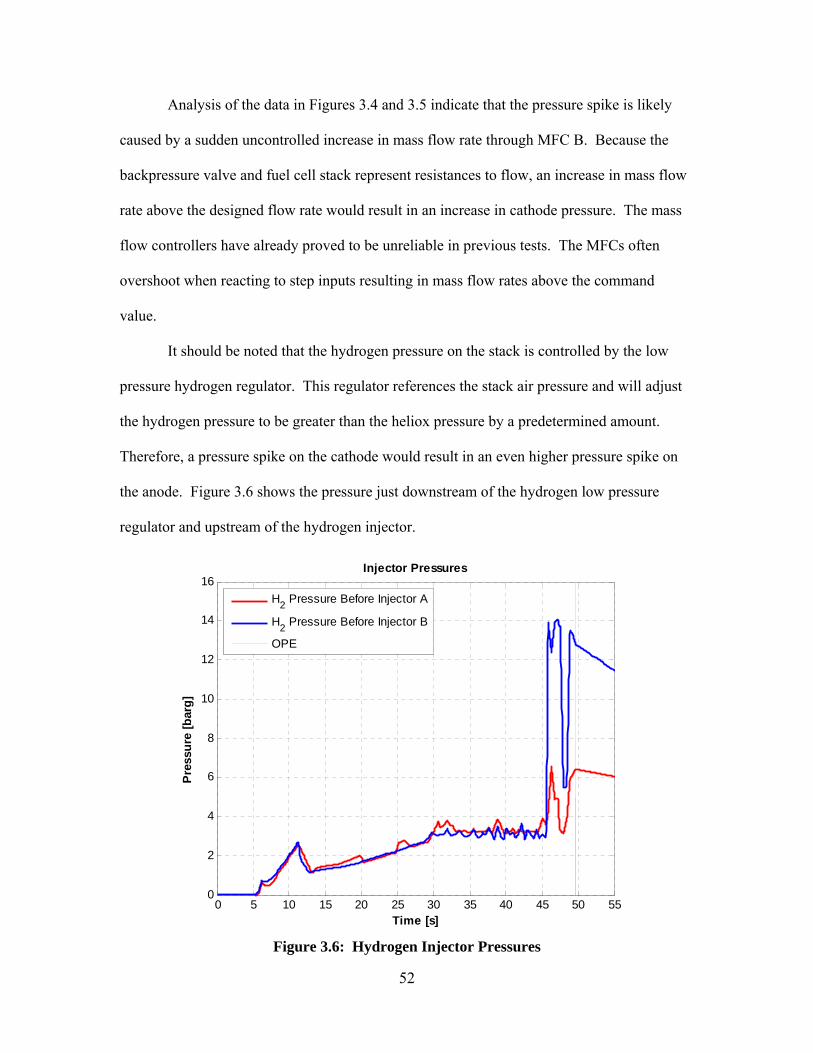
It should be noted that the hydrogen pressure on the stack is controlled by the low
pressure hydrogen regulator. This regulator references the stack air pressure and will adjust
the hydrogen pressure to be greater than the heliox pressure by a predetermined amount.
Therefore, a pressure spike on the cathode would result in an even higher pressure spike on
the anode. Figure 3.6 shows the pressure just downstream of the hydrogen low pressure
regulator and upstream of the hydrogen injector.
Figure 3.6: Hydrogen Injector Pressures
0 5 10 15 20 25 30 35 40 45 50 550
2
4
6
8
10
12
14
16
Time [s]
Pres
sure
[bar
g]
Injector Pressures
H2 Pressure Before Injector A
H2 Pressure Before Injector B
OPE

53
3.4.2 Theoretical Mass Flow Rate through MFC
During the overpressure event the MFC feedback signal was saturated at 150 [g/s] of
heliox, therefore, it is not possible to know how much heliox was actually flowing into the
system. In order to account for the worst case scenario, it can be assumed that the mass flow
through the MFC was governed by the choked flow condition through the MFC orifice. The
equation below describes the gas flow through the mass flow controller for its given flow
coefficient [14]. This equation is used because the large pressure drop across the valve
resulting in sonic choked flow.
1.4711
1.471 6950 6.0 13.51
. 5247 293.15
2.480 4 261.2 /
Where Q = Volumetric Flow Rate [slpm] N2 = Constant based on units [6950] SG = Specific Gravity Cv = Flow Coefficient [6.96] P1 = Upstream Pressure [bar] T1= Upstream Pressure [K]
This suggests that if the mass flow controllers failed in the open position that the
resulting gas flow rate would be 261 [g/s]. This is assuming an upstream pressure of 13.5
[bar]. It should be noted that the upstream pressure was 13.5 [bar] during the overpressure
event in August. However, the upstream pressure was lowered to 9.5 [bar] before the
overpressure event in September. An upstream pressure of 9.5 [bar] would correspond to a
max flow rate of 184 [g/s] of heliox. For the system model developed in the following
section the worst case flow rate of 261 [g/s] from the August overpressure event will be used
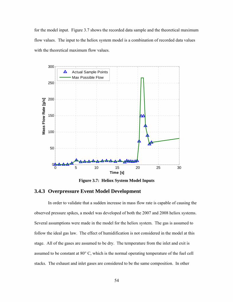
54
for the model input. Figure 3.7 shows the recorded data sample and the theoretical maximum
flow values. The input to the heliox system model is a combination of recorded data values
with the theoretical maximum flow values.
Figure 3.7: Heliox System Model Inputs
3.4.3 Overpressure Event Model Development
In order to validate that a sudden increase in mass flow rate is capable of causing the
observed pressure spikes, a model was developed of both the 2007 and 2008 heliox systems.
Several assumptions were made in the model for the heliox system. The gas is assumed to
follow the ideal gas law. The effect of humidification is not considered in the model at this
stage. All of the gases are assumed to be dry. The temperature from the inlet and exit is
assumed to be constant at 80° C, which is the normal operating temperature of the fuel cell
stacks. The exhaust and inlet gases are considered to be the same composition. In other
0 5 10 15 20 25 300
50
100
150
200
250
300
Time [s]
Mas
s Fl
ow R
ate
[g/s
]
Actual Sample PointsMax Possible Flow
55
words, the oxygen is not consumed through the stack. These assumptions are made because
both overpressure events occurred during low current draw which means that very little
oxygen was consumed and very little produce water was being produced. These assumptions
do reduce the accuracy of the model, however, this model is intended to determine within
relative accuracy whether the system will produce a pressure spike with a given input.
The inlet and exit manifold were modeled using a lumped volume approach. Here
the conservation of mass resulting in:
Adapting this equation into the ideal gas law produces:
Where
m = mass of the gas in the control volume [kg] = mass flow rate in or out of the control volume [kg/s] t = time P = pressure [N/m2] V = volume of the manifold [m3] R = Gas Constant for Heliox [546.9 J/(kg*K)] T = Temperature [K]
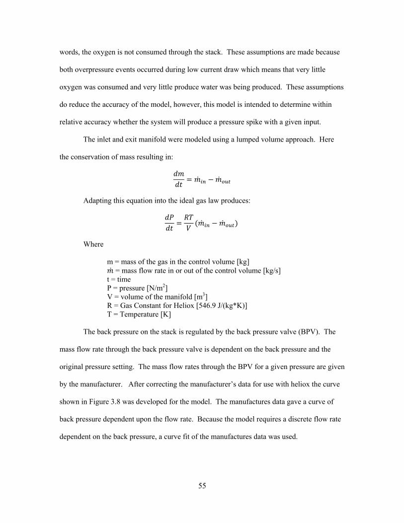
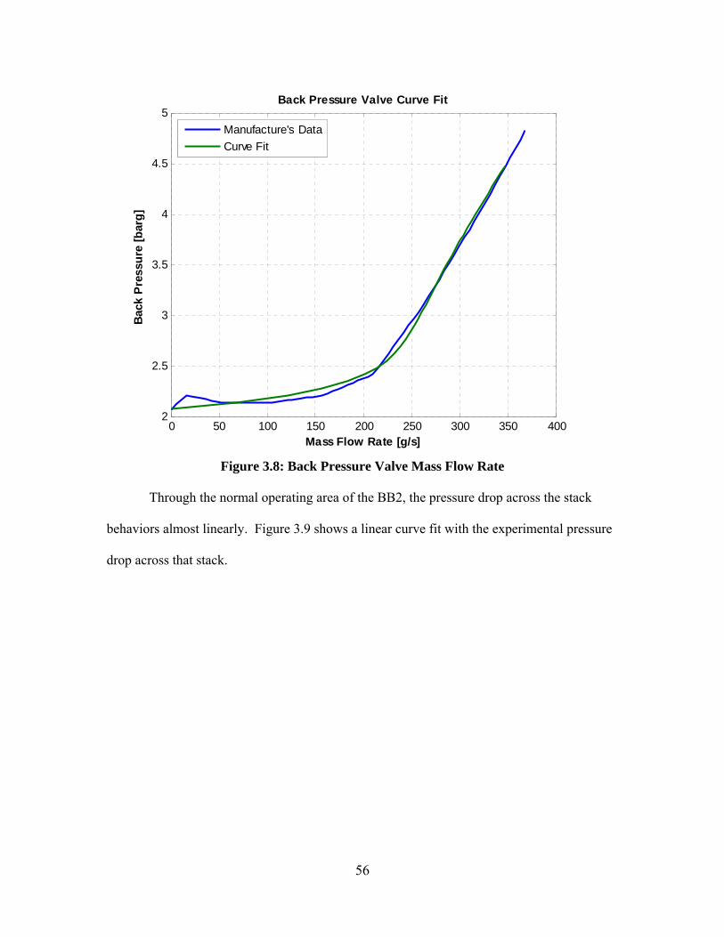
The back pressure on the stack is regulated by the back pressure valve (BPV). The
mass flow rate through the back pressure valve is dependent on the back pressure and the
original pressure setting. The mass flow rates through the BPV for a given pressure are given
by the manufacturer. After correcting the manufacturer’s data for use with heliox the curve
shown in Figure 3.8 was developed for the model. The manufactures data gave a curve of
back pressure dependent upon the flow rate. Because the model requires a discrete flow rate
dependent on the back pressure, a curve fit of the manufactures data was used.
56
Figure 3.8: Back Pressure Valve Mass Flow Rate
Through the normal operating area of the BB2, the pressure drop across the stack
behaviors almost linearly. Figure 3.9 shows a linear curve fit with the experimental pressure
drop across that stack.
0 50 100 150 200 250 300 350 4002
2.5
3
3.5
4
4.5
5Back Pressure Valve Curve Fit
Back
Pre
ssur
e [b
arg]
Mass Flow Rate [g/s]
Manufacture's DataCurve Fit

57
Figure 3.9: Pressure Drop across Cathode
The pressure drop across the stack may not perform linearly during the overpressure
events where the mass flow rate is much higher than the normal operating conditions.
However, the geometry of flow channels inside the stack and other necessary information to
create a more accurate model of the stack is not available to the BB2 team at this time.
Therefore, a linear stack flow resistance will be used for the heliox system model.
The main question to answer in performing this analysis is why there were two over
pressure events in 2008 and no over pressure events in 2007. The overall stack pressure in
2008 was higher than in 2007, however, during normal operation the anode and cathode
pressures remained below the 3.1 [bar] burst pressure of the stack. The only physical
changes to the heliox system between 2007 and 2008 was in the exhaust. In the 2007 the
exhaust from each module entered a single large exhaust tube that ran the length of the car
and exited the rear. In the 2008 exhaust system the overall length and subsequently the
0 10 20 30 40 50 60 70 80 900
0.05
0.1
0.15
0.2
0.25
0.3
0.35
0.4
0.45
Mass Flow Rate [g/s]
Pres
sure
Dro
p ac
ross
Cat
hode
[bar
]
Experimental DataCurve Fit

58
volume of the exhaust was reduced to remove weight. Each module exhausted through a
separate backpressure value. The back pressure was equalized between the modules by a 12.7
[mm] (0.5 [inch]) cross-over tube. The 2007 and 2008 exhaust systems are compared in
Figure 3.10.
Figure 3.10: 2008 and 2007 Exhaust Comparison
For the heliox system model the cross over tube was modeled using compressible
flow with friction through a tube [13]. The flow rate through the tube is dependent on the
ratio between module A and module B back pressure. The resulting curve is shown in figure
3.11. The mass flow rate through the cross over tube increases with increasing pressure ratio.

59
Figure 3.11: Mass Flow Through 12.7 mm Cross Over Tube
For the full Simulink model of the heliox system refer to the Appendix.
3.4.4 Overpressure Event Model Results
Both the 2007 and 2008 system parameters and volumes were integrated into the
heliox system model. The mass flow rate exiting MFC B in the system model is
described by the measured data with the addition of theoretical data where the sensor has
been saturated. The mass flow rate exiting MFC A is the actual mass flow rate measured
from the test data for the September 26 run. Figure 3.12 shows the system inputs used
for the comparison between the 2007 and 2008 systems.
1 1.5 2 2.50
5
10
15
20
25
30
35
40
45Cross Over Tube Flowrate (Pinlet = 2.4 barg)
Pressure Ratio (Pinlet/Pexit)
Mas
s Fl
owra
te [g
/s]

60
Figure 3.12: Heliox System Model Inputs
The results of the system model are shown in Figure 3.13.
0 5 10 15 20 25 300
50
100
150
200
250
300
Time [s]
Mas
s Fl
ow R
ate
[g/s
]
MFC AMFC B

61
Figure 3.13: Heliox System Model Results (2007 and 2008 Comparison)
The model accurately predicts that a pressure spike in the cathode does occur in
module B if the mass flow rate through MFC B does increase to 261 [g/s]. From Figure 3.13
it is obvious that the 2007 system would result in a lower pressure spike with the same mass
flow input and the same stack pressure settings.
Initially it was theorized that the decrease in exhaust volume between 2007 and 2008
was the main contributing factor that lead to the overpressure events. The idea being that a
larger exhaust size gave the system a larger capacitance and the short duration increase in the
0 5 10 15 20 25 302
2.5
3
3.5
4
4.5
Stac
k In
let P
ress
ure
[bar
]
0 5 10 15 20 25 302
2.2
2.4
2.6
2.8
3
Time [s]
Back
Pre
ssur
e [b
ar]
Inlet Pressure A 2007Inlet Pressure B 2007Inlet Pressure A 2008Inlet Pressure B 2008
Back Pressure 2007 A and BBack Pressure 2008 ABack Pressure 2008 B

62
mass flow rate would not significantly increase the back pressure. However, increasing the
volume in the 2008 model showed very little difference in output pressure.
It is more likely that the effect of having the excess flow regulated by two back
pressure valves in the 2007 system as opposed to the individual valves in the 2008 system
was the cause of pressure spike. Again, in the 2007 system the exhaust exited both fuel cell
modules and entered a common exhaust tube. Two back pressure valves were placed
downstream of this common exhaust. In the 2008 system the module exhausted through
individual back pressure valves. The back pressure was intended to be equalized using a 12.7
[mm] (0.5 [in]) cross over tube between the two exhaust tubes. The Simulink model shows
that the 12.7 [mm] cross over tube does not adequately equalize pressure between the two
modules. Therefore, the increased mass flow through FCM B is not completely shared with
the BPV for FCM A. The mass flow rates through each BPV and the cross over tube are
shown in Figure 3.14.
Increasing the size of the cross over tube aids in increasing the cross over flow rate
and subsequently equalizing the pressure between module A and B. Figure 3.15 shows
resistance values for various sized cross over tubes. Increasing the cross over tube diameter
to 50.8 [mm] (2.0 [in]) effectively equalizes pressure between module A and B. The pressure
varies by less than 1% between the two exhaust pressures with a 50.8 [mm] cross over tube.
This means that the model solution for the 2008 system with a 50.8 [mm] cross over tube
approaches 2007 model results. Figure 3.16 shows a comparison between the 2007 system
and the 2008 system with a 50.8 [mm] cross over tube.

63
Figure 3.14: Heliox Mass Flow Rates Through BPVs and Cross over Tube
Figure 3.15: Cross Over Tube Flow Rate with Varying Diameter
0 5 10 15 20 25 30-50
0
50
100
150
200
250
Time
Mas
s Fl
ow R
ate
[g/s
]
BPV ABPV BCross over Tube
1 1.5 2 2.50
200
400
600
800
1000
1200Cross Over Tube Flowrate (Pinlet = 2.4 barg)
Pressure Ratio (Pinlet/Pexit)
Mas
s Fl
owra
te [g
/s]
0.5 [in] Cross Over Tube1.0 [in] Cross Over Tube2.0 [in] Cross Over Tube

64
Figure 3.16: 2007 Heliox System and 2008 Heliox System with 50.8 [mm] Cross Over
Tube Simulation Results Comparison
These results indicate that the 2008 exhaust setup with a 50.8 [mm] cross over tube
does have comparable performance to the 2007 system. However, the model still indicates a
pressure spike above 3.1 [bar] which is the rated burst pressure of the stacks. These results
are obtained considering an operating inlet cathode pressure of 2.4 [bar] which reflects the
2008 pressure settings. The overall stack pressure could be reduced to account for this
potential overshoots in the mass flow rate. However, this would decrease the fuel cell’s
0 5 10 15 20 25 302
2.5
3
3.5
Time [s]
Inle
t Pre
ssur
e [b
ar]
0 5 10 15 20 25 302
2.1
2.2
2.3
2.4
2.5
2.6
2.7
Time [s]
Exha
ust P
ress
ure
[bar
]
FCM A (2.0 [in] cross over tube)FCM B (2.0 [in] cross over tube)FCM A (2007 system)FCM B (2007 system)
FCM A (2.0 [in] cross over tube)FCM B (2.0 [in] cross over tube)FCM A (2007 system)
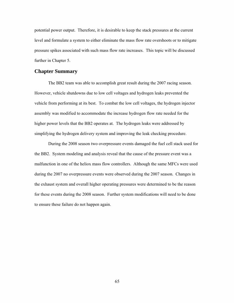
65
potential power output. Therefore, it is desirable to keep the stack pressures at the current
level and formulate a system to either eliminate the mass flow rate overshoots or to mitigate
pressure spikes associated with such mass flow rate increases. This topic will be discussed
further in Chapter 5.
Chapter Summary
The BB2 team was able to accomplish great result during the 2007 racing season.
However, vehicle shutdowns due to low cell voltages and hydrogen leaks prevented the
vehicle from performing at its best. To combat the low cell voltages, the hydrogen injector
assembly was modified to accommodate the increase hydrogen flow rate needed for the
higher power levels that the BB2 operates at. The hydrogen leaks were addressed by
simplifying the hydrogen delivery system and improving the leak checking procedure.
During the 2008 season two overpressure events damaged the fuel cell stack used for
the BB2. System modeling and analysis reveal that the cause of the pressure event was a
malfunction in one of the heliox mass flow controllers. Although the same MFCs were used
during the 2007 no overpressure events were observed during the 2007 season. Changes in
the exhaust system and overall higher operating pressures were determined to be the reason
for these events during the 2008 season. Further system modifications will need to be done
to ensure these failure do not happen again.

66
Chapter 4 :
Performance Results
The main focus of this research is to improve the reliability and performance of the
Ballard power plant used in the BB2. Large amounts of data are recorded during each run
and test session. Being able to identify factors that characterize a good run and a bad run are
essential. From a passenger car perspective, there are many considerations when judging the
performance of a fuel cell system. Such systems are designed to balance power output,
efficiency, cost, durability, longevity, safety and reliability. For the BB2 fuel cell system,
safety, of course, remains the principle criteria when analyzing post run results. The second
important criteria would be the power output. Modeling of the stack is important for gauging
the effect of changes on overall stack performance.
The stack model developed in this thesis is used in the overall vehicle simulator as
well as in the vehicle control code. This model helps to determine the theoretical top speed
of the vehicle. It can also be used to determine the amount of ice necessary to cool the
vehicle during a run. Additionally the vehicle gear ratios are determined by using the
simulator.
4.1 Fuel Cell Model
There are many models that have been developed in the literature for fuel cells.
These models vary greatly in their complexity and modeling approach. The type of model
and complexity level needs to match the function, resources and desired data for the specific

67
project. For the BB2 the model and polarization curves are used for determining
performance and power output. Also the polarization curves are used in overall vehicle
modeling which is used to determine the top speed of the vehicle, cooling strategy and gear
ratios. Also the polarization curve is used in the control for determine the current request.
The model is not used for prediction of fuel cell stack performance outside of the testing
conditions. This reduces the required complexity of the model. Many of the required
specifications for complex mechanistic models are not know to the BB2 team. Therefore, an
empirical model will be adopted for the use of the BB2 project.
4.1.1 Fuel Cell Model Definition
Hydrogen fuel cells combine hydrogen and oxygen to form water. The overall
reaction that takes place in a fuel cell is described by the following equation:
12
Based on this equation and thermodynamic principles, the ideal cell voltage can be
characterized by the Nerst Equation which is as follows [9]:
2 ln .
Where:
E = thermodynamic equilibrium potential [V] Eo = reference potential [V] R = gas constant (8.3143 [J/(mol*K)]) T = temperature [K] F = Faraday’s constant (96485 [C/mol]) PH2* = partial pressure of hydrogen [atm] PO2* = partial pressure of oxygen [atm]
This equation reduces to [15]:
1.229 8.5 10 298.15 4.3085 10 ln 0.5 ln

68
This potential represents the ideal cell voltage under no load. The actual cell voltage
is the sum of the ideal voltage and the sum of the losses. The three primary losses for a fuel
cell are the activation, ohmic and concentration losses.
Activation losses are a result of the voltage lost in driving the chemical reaction that
transfers the electrons to or from the electrode [9]. For the BB2, there are several ways to
decrease the activation losses. Raising the cell temperature increases the rate of reaction at
the anode and cathode and thus decreases the activation losses. Increasing the reactant
concentrations decreases the activation losses by more efficiently occupying catalyst sites.
Increasing the concentration of reactants can be achieved either by increasing the mole
fraction of the reactant within the mixture (not applicable for the anode because the hydrogen
concentration is already 100%) or by increasing the pressure. Additionally MEA designers
can decrease activation losses by using more effective catalysts and increasing the roughness
of the electrodes which increases the surface area and subsequently increases catalyst
reaction sites [9].
Ohmic losses are caused by the internal resistance of the stack materials to the flow
of electrons. These losses are the same as any electrical resistive losses in electrical systems.
These losses can be minimized by using electrodes and other conductive components with
the high conductivity and making the electrolyte as thin as possible [9].
Concentration losses or sometimes referred to as mass transport losses are the result
of the change in concentration of the reactants at the surface of the electrodes as the fuel is
used [16]. These losses can be minimized by increasing pressure and reactant concentration.
Figure 4.1 depicts the typical polarization curve for a PEM fuel cell. From the figure,
it can be seen that activation losses dominate the behavior of the polarization curve under low
current draw. The ohmic losses then determine the behavior in the middle portion.
Concentration losses dominate the very high current draw.

69
Figure 4.1: Generic Polarization Curve for a PEM Fuel Cell [17]
From experimental data the BB2 does not appear to enter this region where
concentration losses dominate. Therefore the modeling of the stack will ignore these losses.
In doing so the trends and power curves obtained from the experimental data will accurately
capture the performance of the modeling within the experimentally tested ranges. However,
the acquired data will not accurately predict fuel cell performance above these values.
The total fuel cell voltage can be characterized by the sum of the ideal open circuit
voltage with the activation and ohmic losses [15]:
Where:
V = cell voltage [V] E = thermodynamic potential as described by the Nerst Equation [V] ηact total = total activation losses [V]
ηact total = total ohmic losses [V]

70
The total activation losses are a sum of the activation losses at the cathode and anode:
Again, the individual parameters for the stack to mechanically determine the anode
and cathode activation losses independently are not know. Therefore, the anodic and
cathodic activation losses will be lumped together in one expression. The value for the total
activation losses can be determined empirically from the following formula [15]:
ln ln
Where:
ξ1, ξ2,ξ3, ξ4 = parametric coefficients T = temperature [K] cO2*=concentration of oxygen [mol/cm3] i = Current [A]
The oxygen concentration on the cathode is dependent on the partial pressure of the
oxygen and the temperature. It can be determined by the following equation[15]:
5.08 10 exp 498
Where PO2 is that partial pressure of oxygen. The temperature and pressures used to
develop this model will be taken at the average across the stack. This simplification is
adequate for the purposes of this empirical model.
The ohmic losses are a function of the internal resistance, Rinternal, of the stack and the
current draw. The ohmic losses can be determined by the following equation:
Where the internal resistance, Rinternal, is determined by the following parametric
equation[15]:
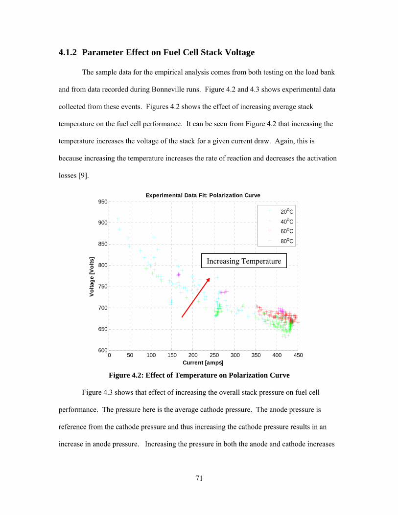
71
4.1.2 Parameter Effect on Fuel Cell Stack Voltage
The sample data for the empirical analysis comes from both testing on the load bank
and from data recorded during Bonneville runs. Figure 4.2 and 4.3 shows experimental data
collected from these events. Figures 4.2 shows the effect of increasing average stack
temperature on the fuel cell performance. It can be seen from Figure 4.2 that increasing the
temperature increases the voltage of the stack for a given current draw. Again, this is
because increasing the temperature increases the rate of reaction and decreases the activation
losses [9].
Figure 4.2: Effect of Temperature on Polarization Curve
Figure 4.3 shows that effect of increasing the overall stack pressure on fuel cell
performance. The pressure here is the average cathode pressure. The anode pressure is
reference from the cathode pressure and thus increasing the cathode pressure results in an
increase in anode pressure. Increasing the pressure in both the anode and cathode increases
0 50 100 150 200 250 300 350 400 450600
650
700
750
800
850
900
950Experimental Data Fit: Polarization Curve
Current [amps]
Vol
tage
[Vol
ts]
20oC
40oC
60oC
80oC
Increasing Temperature

72
the concentration of reactants and increases the catalyst site utilization. This increases the
overall stack voltage.
Figure 4.3: Effect of Pressure on Polarization Curve
One of the major advantages that the BB2 has over other fuel cell vehicles is that the
BB2 carries its own oxidant on board. This allows that BB2 to run on higher concentrations
of oxygen than the surrounding air. Figure 4.4 shows the effect of increasing the oxygen
concentration. This data was obtained from short stack testing performed at Ballard. Regular
air, heliox and pure oxygen were used for the test. The test clearly indicates that pure oxygen
has the highest voltage for a given current draw. However, pure oxygen is very dangerous.
At high pressure even stainless steel is flammable in the presence of pure oxygen. Therefore,
the BB2 uses a safer concentration of 40% oxygen to 60% helium.
0 50 100 150 200 250 300 350 400 450600
650
700
750
800
850
900
950Experimental Data Fit: Polarization Curve
Current [amps]
Vol
tage
[Vol
ts]
P<2.02.2>P>2.02.4>P>2.22.6>P>2.42.6>P
Increasing Pressure

73
Figure 4.4: Oxygen Concentration Effect on Stack Performance
4.1.3 Model Results
The empirical equations described in section 4.1.1 were solved using the least squares
linear regression method. The values obtained for ξ1-7 are shown in Table 4.1 and 4.2.
ξ1 0.8097 ξ2 -6.473*10-3 ξ3 -3.076*10-4 ξ4 1.533*10-4
Table 4.1: Activation Losses Empirical Constants
ξ5 9.190*10-4 ξ6 -1.985*10-6 ξ7 1.003*10-7
Table 4.2: Ohmic Losses Empirical Constants
The breakdown of the activation and ohmic loss components of the total voltage
reduction are shown graphically in Figure 4.5. The model clearly shows that the activation
0 100 200 300 400 500 600 700 800 900550
600
650
700
750
800
850
900
950
1000
1050Short Stack Testing
Current [amps]
Volta
ge [V
olts
]
Air (20.9% O2)
Heliox (40% O2)
100% O2

74
losses build quickly at low current values and then remain mostly constant at mid to high
current levels. The ohmic losses build steadily throughout the current range.
Figure 4.5: Activation and Ohmic Losses
The resulting polarization curve from the model is displayed in Figure 4.6. The
power generated by the fuel cells is given in Figure 4.7. Each figure gives the model voltage
for a given current as a function of temperature. The temperature of the fuel cell stack varies
throughout the run. The stacks start out at 20°C at the beginning of the run. The stack then
heats up as the run progresses. The stacks are actively cooled to maintain 80°C as the
maximum operating temperature. From Figure 4.7, the model indicates that at 80°C the
maximum power output of the stack is close to 600 [kW]. This matches the maximum power
observed during load cell testing.
0 100 200 300 400 500 600 700 800 9000
50
100
150
200
250
300
350
400
450
Current [Amps]
Volta
ge L
oss
[V]
Vact at 20oC
Vohm at 20oC
Vact at 40oC
Vohm at 40oC
Vact at 60oC
Vohm at 60oC
Vact at 80oC
Vohm at 80oC
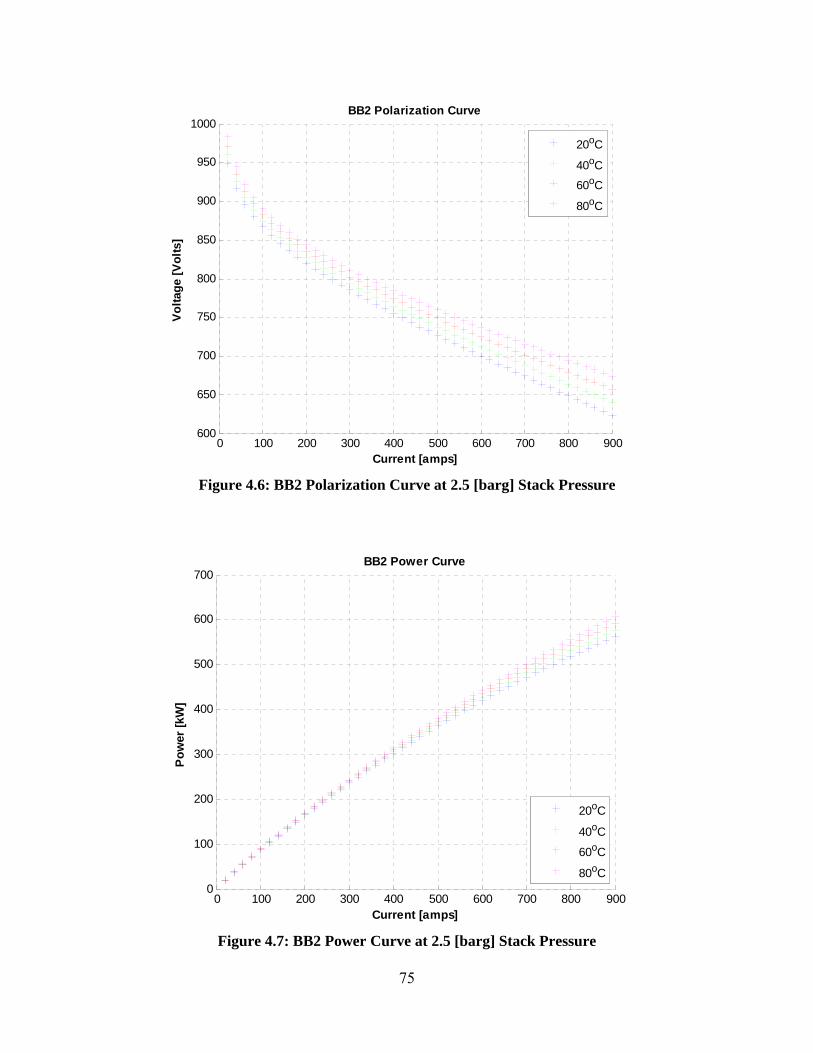
75
Figure 4.6: BB2 Polarization Curve at 2.5 [barg] Stack Pressure
Figure 4.7: BB2 Power Curve at 2.5 [barg] Stack Pressure
0 100 200 300 400 500 600 700 800 900600
650
700
750
800
850
900
950
1000BB2 Polarization Curve
Current [amps]
Volta
ge [V
olts
]
20oC
40oC
60oC
80oC
0 100 200 300 400 500 600 700 800 9000
100
200
300
400
500
600
700
Pow
er [k
W]
BB2 Power Curve
Current [amps]
20oC
40oC
60oC
80oC

76
The main focus of the testing during the 2008 season was to increase the fuel cell
reliablility. This was certainly accomplished. During Speedweek 2008 there were no fuel
cell system related vehicle shutdowns the first four days of racing. In addition to improved
reliability the team was able to improve the performance and maximum power output of the
Ballard P5 FCMs. Figure 4.8 shows a comparison of the theoretical polarization curve for
the 2007 and 2008 racing season. Figure 4.9 shows a comparison of the corresponding
power curve for the 2007 and 2008 season. For these figures the 2008 data was obtained
from the model previously discussed. The 2007 curves were obtained from empirical values
determined in [6]. Both were calculated using a stack pressure of 2.5 bar at 80°C. The
improvement in the overall stack performance can be attributed to several changes. The most
significant change would be in the increased hydrogen flow rate at high current.

77
Figure 4.8: BB2 2007 vs. 2008 Polarization Curve Comparison
Figure 4.9: BB2 2007 vs. 2008 Power Curve Comparison
0 100 200 300 400 500 600 700 800 900550
600
650
700
750
800
850
900
950
1000
Current [amps]
Volta
ge [V
olts
]
20082007
0 100 200 300 400 500 600 700 800 9000
100
200
300
400
500
600
700
Current [amps]
Pow
er [k
W]
20082007

78
4.2 Fuel Cell Model Application
The fuel cell model developed in this thesis is used for several reasons. The
empirical constants that are determined for the fuel cell performance can be input into the
total vehicle model for use to determine the vehicle’s theoretical top speed. For more
information able the BB2’s total vehicle model and its development refer to [6].
The theoretical polarization curve is also utilized by the vehicle’s control code.
The Motohawk controller receives input from the driver and requests a certain current
level from the Ballard controller. The Ballard controller uses the current request to
determine the mass flow rate of the heliox and other system parameters. The throttle
input of the driver corresponds to the percent of maximum power based on the motor’s
power/speed curve. This desired power is then converter to a current request using the
theoretical polarization curve. Figure 4.10 shows the current request algorithm for the
Buckeye Bullet 2.
Figure 4.10: BB2 Current Request Algorithm
3CAN - Current Command
2Current Request
1Power Max
RPM 2 Power
1
Power Speed Scale
Power 2 CurrentMultiply2
Alpha45 <= I <= 900
400 <= RPM <= 10500
3Software Power Limit
2Motor RPM
1AI - Throttle

79
4.3 2008 Season Results
2008 was the second racing season for the Buckeye Bullet 2. The 2007 season
proved to be a great learning experience for the team. Setting a world record in the first year
and achieving the fastest recorded speed for a hydrogen fuel cell powered vehicle are great
accomplishments. However, there were many issues with the vehicle that needed to be
address before the 2008 season if the team hoped to reach its goals of 300 mph. The BB2
raced twice during 2008; once in August during Speedweek and once in September during a
private FIA meet.
4.3.1 Speed Week 2008
The Buckeye Bullet 2’s first race event in 2008 was Speedweek. The main goal for
this meet was to prove the reliability of the fuel cell system. Before the first run several spin
tests were performed in the pit area to ensure that all systems were functioning properly on
the salt. The first run on the salt for that season occurred on August 19. This first run
resulted in a blistering 338 [km/h] (210 [mph]) speed recorded by the SCTA. This was a
great way to start of the week. However, during this run the vehicle was not shutdown by the
driver. The vehicle shutdown due to faulty emergency power off (EPO) switch. The EPO
switch is an electrical switch at the rear of the vehicle that allows a team member or safety
personal to cut power to the vehicle in the event of an emergency. The switch disconnects
power from the batteries to the fuel cell systems. This effectively closes the tank solenoids
and stops the fuel cells.
Several more run attempts were made with the faulty EPO switch before the failure
was properly identified. The EPO switch is required by SCTA rules; therefore, an
improvised replacement EPO switch was installed. On the morning of August 21, the
following run with the properly working EPO switch resulted in the vehicle reaching 360

80
[km/h] (224 [mph]) recorded by the SCTA. This run was ended by a premature deployment
of the vehicle’s parachutes. For ease of operation all driver controls are placed on the
steering wheel. This allows the driver to keep his hands on the wheel at all times. However,
during the run the driver inadvertently pushed the parachute release button rather than the
upshift button.
The course was shut down due to high winds so the next run was not until August 22.
The following run was the fastest run for the BB2 ever recorded. The top speed measured by
the SCTA was 461.024 [km/h] (286.467 [mph]) at the exit of the 5th mile. The top speed
measured by the vehicles onboard GPS system after the final timed mile was 478 [km/h] (297
[mph]). The fuel cell produced 560 kW during the run. All of the vehicle systems worked
flawlessly. The vehicle’s power was limited to 560 kW during the run by the inverter
settings. Until this time the inverter had not been the limiting factor. The fuel cells had
successfully reached over 600 kW of power during testing, therefore, it was known that the
car had more to give. Now with the fuel cell systems and other vehicle systems working
perfectly it was necessary to increase the inverter limits to increase the power draw from the
fuel cell modules.
The inverter settings were increased from 80% torque limit to 90% torque limit. The
subsequent run resulted in a vehicle shutdown due to an inverter fault. The following two
runs the inverter was limited back to 85% and 83% respectively. Both runs resulted in
inverter faults and shutdowns. It should be noted that throughout the week up to this point
there were no fuel cell related shutdowns. The reliability and performance of the fuel cell
systems had been verified. At this point the fuel cell system was no longer the limiting factor
in the power production.
On second run on August 23 a low humidification pump pressure caused a fuel cell
system shutdown. The third and final run on August 23 resulted in an overpressure event that

81
caused a leak in stack B. The failure was caused by a malfunction in MFC B that resulted in a
large overshoot in mass flow rate that lead to a pressure spike. Detailed analysis of this event
is discussed in chapter 3. This event ended Speedweek for BB2 team as a stack leak is not
field serviceable. A summary of the runs completed during Speedweek 2008 is shown in
Table 4.3. It should be noted that the peak speed presented in this table is recorded from the
vehicle’s GPS data and may not match the peak speed as recorded by the SCTA.
Run No. Date Peak Speed Peak Power Run end condition 1 August 19 360 km/h 553 kW Shutdown due to faulty EPO switch 2 August 20 63 km/h 178 kW Shutdown due to faulty EPO switch 3 August 21 365 km/h 550 kW Early parachute deployment 4 August 22 478 km/h 560 kW No faults 5 August 22 375 km/h 590 kW Shutdown from inverter over-current 6 August 22 455 km/h 589 kW Shutdown from inverter over-current 7 August 23 460 km/h 588 kW Shutdown from inverter over-current
Table 4.3: Run Summary for 2008 Racing Season [7]
4.3.2 FIA Meet 2008
The stack leak that occurred in August could only be repaired at the Ballard facilities
in Vancouver. The FIA meet began on September 22, 2008. This meant that FCM B had to
be shipped to Vancouver, serviced, shipped back to Ohio and installed into the vehicle in less
than one month. The task was completed with the diligence and dedication of BB2 team
members and Ballard personnel. However, the absence of the FCM made testing the fuel cell
system, inverter and motor almost impossible in-between the two racing events. Therefore,
after the fuel cell system was repaired an installed into the vehicle it was shipped to the salt
flats without testing.
Upon arrival to the salt flats during the FIA meet in 2008 it was discovered that the
vehicle had a very serious failure. The custom made motor had an internal short between the
rotor and stator that made the motor unusable. Disassembly of the motor at a shop in Utah
revealed that the carbon fiber windings that surround part of the rotor had frayed and shorted
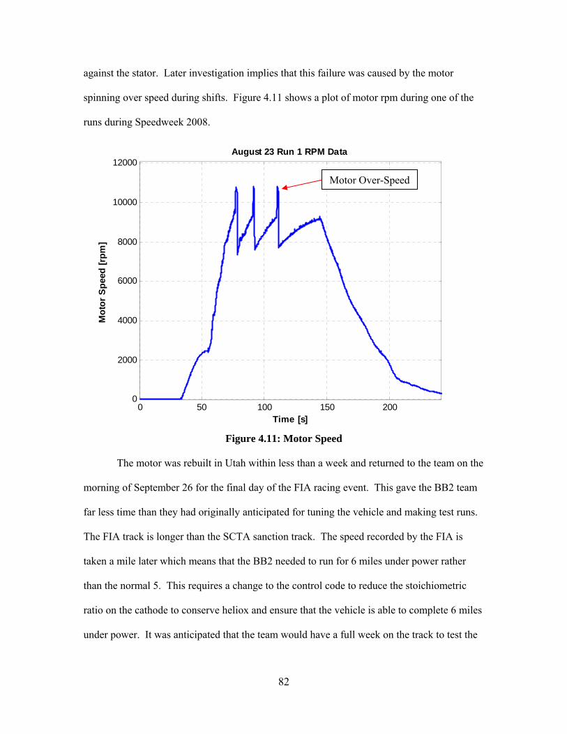
82
against the stator. Later investigation implies that this failure was caused by the motor
spinning over speed during shifts. Figure 4.11 shows a plot of motor rpm during one of the
runs during Speedweek 2008.
Figure 4.11: Motor Speed
The motor was rebuilt in Utah within less than a week and returned to the team on the
morning of September 26 for the final day of the FIA racing event. This gave the BB2 team
far less time than they had originally anticipated for tuning the vehicle and making test runs.
The FIA track is longer than the SCTA sanction track. The speed recorded by the FIA is
taken a mile later which means that the BB2 needed to run for 6 miles under power rather
than the normal 5. This requires a change to the control code to reduce the stoichiometric
ratio on the cathode to conserve heliox and ensure that the vehicle is able to complete 6 miles
under power. It was anticipated that the team would have a full week on the track to test the
0 50 100 150 2000
2000
4000
6000
8000
10000
12000August 23 Run 1 RPM Data
Time [s]
Mot
or S
peed
[rpm
]
Motor Over-Speed

83
necessary changes and make adjustments. However, with the motor failure an entire week of
testing and racing had to be compressed into one day of racing.
The team was able to complete 4 runs on August 26th. The first run on the 26th was
aborted due to a control code issue that resulted in a failure to properly open the hydrogen
tank solenoid. The hydrogen tank contains a safety system that will not permit high flow if
the pressure difference inside the tank and the connecting line is too great. This ensures that
if a significant leak occurs that hydrogen tank will restrict large flow rates. This means that
the control code must pressurize the hydrogen line before significant hydrogen flow rates. A
coding error caused prevented the line from properly pressurizing at the start and thus the
tank solenoids did not fully open.
After fixing the coding issue, the next two runs were aborted due to individual low
cell voltages. The exact cause of these low cells is not certain at this time. However, there
are several possible answers. During these runs the purge solenoid is commanded to say
open. This can happen for several reasons. The purge solenoid can be held open if the
hydrogen pressure is too high or if the stack has some low cell. The solenoid opens for low
cells in an effort to purge contaminants out of the anode and increase the hydrogen
concentration. However, for the BB2 low cells are usually not caused by anode contaminants
because the runs last for such a short time that there is not much time for contaminants to
leak over from the cathode. For the BB2, most low cells are caused by low hydrogen
pressure on the anode. Therefore opening purge makes this problem worst. The other
scenario is that the purge is held open to reduce hydrogen pressure on the stack because the
pressure is too high.
The final run on August 26th resulted in another overpressure event. MFC B
malfunctioned and overshot the mass flow command resulting in a pressure spike on the
cathode. Because the anode pressure references the cathode, the pressure on the anode

84
increased as well. The high pressure on the anode and cathode blew one of the stack seals on
module B. The escaping heliox and hydrogen ignited and caused minor damage to the
vehicle’s body panels and fuel cell module panels. All other major vehicle systems and the
driver were unharmed.
The fuel cell system that proved to be almost bullet proof during Speedweek showed
that it clearly still has room for improvement.
Chapter Summary
This chapter describes the approach used for modeling the BB2 fuel cell stack. The
fuel cell voltage at any current draw is determined to be the sum of the ideal stack voltage
and the activation and ohmic losses. Empirical methods were used to determine the voltage
losses and how they are affected by temperature, pressure, current draw, and reactant
concentration.
Changes made to the vehicle during the 2008 season drastically improved the fuel
cell system reliability. This allowed the team to achieve a top recorded speed of 461.024
[km/h] (286.467 [mph]) during Speedweek 2008. However, failures occurring both during
Speedweek and the private FIA week show the need for further improvement.

85
Chapter 5 :
Conclusion and Future Work
This chapter provides a summary and conclusion of the work presented in this thesis.
It also outlines future work to be done on the vehicle and the fuel cell systems. The majority
of the future work centers around addressing the overpressure events that occurred in 2008
and redesigning the system to eliminate this failure. This section also proposes several other
changes to the vehicle such as removing the fuel cell humidification system and making a
new motor.
5.1 Conclusion of Work
In two short years the Buckeye Bullet 2 has become the fastest hydrogen fuel cell
powered vehicle. This is an incredible feat considering that the students working on the
project only do so part time and attend a full course load of classes through much of the year.
Although the team receives support from industry supports, the students on the team still
remain the ultimate facilitators of the project.
Tremendous progress has been made with the vehicle between 2007 and 2008. In the
2007 season the vehicle had many issues that caused it to shut down. The primary issue was
hydrogen starvation at the stack. This problem was addressed by modifying the hydrogen
supply system to the stack to allow for high flow. The hydrogen injectors nozzles were
increased in size to accommodate 500 [amps] per module.
Another major area of improvement over the 2008 season was with vehicle weight
reduction. The majority of weight was removed from the gas delivery system, cooling

86
system and fuel cell modules. The total weight reduction reduced the vehicle weight by
roughly 8%.
The 2008 season saw a great improvement for the BB2. The fuel cell system
performed very reliably during Speedweek 2008. An unfortunate motor failure and a
shortened timeline for racing resulted in a disappointing FIA meet in 2008. Both events
ended with an overpressure event that damaged FCM B.
The cause of this overpressure event has been identified as a malfunction of the mass
flow controller for module B. Changes to the exhaust system and an overall higher stack
pressure between 2007 and 2008 increased the system sensitivity to increased mass flow rate
inputs. However, the following section will outline future plans to mitigate these failures.
5.2 Future Work
Although the Buckeye Bullet has come a long way in development since the project
was first start in 2004, there are still areas of the vehicle design that need to be addressed.
The heliox system needs to be revised to eliminate the possibility of pressure spikes that can
damage the stack seals. Additionally there may be potential for further weight reduction by
removal of the humidification system. Also, development of a new or modified motor might
improve power delivery to the driveline.
5.2.1 Possible Heliox System Revisions
It is evident from the model results shown in Chapter 3 that if a significantly higher
than designed mass flow rate of heliox enters the stack that a dangerous pressure increase can
occur. There are two main avenues to address this issue. One would be to allow the system
to release this pressure to eliminate the possibility of damage to the stack. The other
possibility would be to eliminate that possibility of having such a high mass flow rate.

87
The first methodology would require the least amount of modification to the current
system. This would entail installing some kind of pressure relief device on the heliox inlet of
the stack to release pressure in the case of a pressure surge. The current heliox system model
can be used to accurately assess the performance of such a system and determine the
necessary flow capacity and pressure setting of the pressure relief device. Figure 5.1 shows
one possible heliox system with a PRV at the inlet.
Figure 5.1: Possible Heliox System Redesign with Pressure Relief Valves
The second method for eliminating pressure spikes in the air system would be to
eliminate the potential to flow above normal flow rates. It is not clear exactly what causes
the MFCs to overshoot. It might be an issue with their software that causes overshoot in the
control system. It has been shown in testing that the MFCs are susceptible to moisture and
salt. Corrosion and water intrusion will cause undesired flow rates through the MFCs.
Another possibility is that the MFCs are susceptible to the vibrations they endure during a
run. Whatever the cause for the MFC failure it is not within the abilities of the BB2 team to
modify or redesign the MFC to eliminate the possibility of overshoot. Therefore, the only
way to eliminate the potential to have uncontrolled jumps in flow rate is to eliminate the mass
flow controllers from the system altogether.

88
The Ford 999 used a system of metering valves under choked flow conditions to
regulate the flow of heliox through the stack. The system consisted of an idle flow orifice
and a high flow orifice. Solenoid valves where used to actuate the high flow orifices. A
similar system could be adapted to replace the mass flow controllers. This is possible
because the vehicle only spends a short period of time at low power levels. 85% of the run is
spent at full power. However, this would slightly increase the overall heliox consumption
because more heliox would be wasted at the beginning of the run. This is a concern because
during the 2008 season the vehicle ran out of heliox just after the 5th mile which is adequate
for the SCTA course but too short for the FIA course. Although the stoichiometric ratio
could be adjusted to use less heliox this should only be considered as a last resort because
low stoich ratios can negatively affect fuel cell performance.
One option to address heliox consumption for this type of system would be to
increase the number of metering valves. A system with three different sized orifices could
generate 8 discrete flow levels. This would allow the vehicle to use heliox more efficiently
and makes this system more attractive. However, this system would take much more
development time and testing compared to simply installing a pressure relief valve. The
system currently performs well with the MFCs and changing the system entirely at this stage
in the project may not be worth the additional effort. Figure 5.2 shows a potential system
redesign using three metering valves.

89
Figure 5.2: Possible Heliox System Redesign with Metering Valves
5.2.2 Removal of Fuel Cell Humidification System
Water management is very important in fuel cell systems. Water is not only a
product of the reaction but also essential for the reaction to take place. Water allows the H+
ions to travel through the PEM membrane. As the water content falls, the conductivity falls
in a more or less linear fashion [9]. However, if there is too much water in the stack this can
cause flooding in the stack as previously discussed in chapter 3. Therefore control of the
humidification system is very important in fuel cell systems to ensure that the membranes are
hydrated to the appropriate amount.
One potential area for further weight reduction is the humidification system for the
BB2. The Ford 999 did not use an onboard humidification system. Rather they conditioned
the cells while stationary using a separate humidification system. Then during the run they
relied on the product water creation to provide adequate humidification. The water produced
in the reaction is directly proportional to the current draw. At 880 [Amps] the fuel cells are
producing 78.9 [g/s] of water during the reaction. Removing the system would reduce weight
and complexity in the system. Less complexity would mean there are less components to
fail. Several failures in the 2008 testing season were linked to the humidification system.
Further testing will be necessary to see if this is feasible for the BB2.

90
5.2.3 New Motor
The next major area of development for the BB2 will be in the motor and inverter.
The motor used for the BB2 is the same one that was used in the original Buckeye Bullet.
The motor was initially design for a higher voltage and lower current than what is ideal for
the BB2. One of the main issues during Speedweek 2008 was that the motor was not able to
draw the fuel cell’s maximum amount of power. Further dynamometer testing will be
necessary to determine whether the current motor and inverter are capable of drawing 600
[kW] at 680 [V] on the DC side.
If the current motor is not capable of this objective, it is possible to rewind the motor
and design is such that it produces the same power at a lower voltage and higher current.
This would allow the full 600 [kW] to be drawn from the fuel cells and increase power over a
larger RPM range.
91
References
[1] 2007 Rules and Record. Southen California Timing Association. 2007 [2] Göschel Burkhard. BMW’s Drivetrain for Tomorrow. Automotive Engineering
International, January 2005. [3] Serious Wheels. [Online] www.seriouswheels.com. [4] Ford sets land speed record with fuel cell racecar. Fuel Cells Bulletin. Volume 2007,
Issue 10, October 2007. [5] Hillstrom, Edward. Investigation of Chassis Rigidity and Vehicle Handling of an
Electric Land Speed Vehicle. The Ohio State University. 2003. [6] Sinsheimer, Benjamin. Design and Simulation of a Fuel Cell Land Speed Vehicle
Propulsion System. The Ohio State University. 2008. [7] Ponziani, Kevin. Control System Design and Optimization for the Fuel Cell Powered
Buckeye Bullet 2 Land Speed Vehicle. The Ohio State University. 2008. [8] Wright, Benjamin. Development and Modeling of a Suspension for the Ohio State
Buckeye Bullet 2. The Ohio State University. 2006 [9] J. Larminie, A. Dicks. Fuel Cell Systems Explained. New York: Wiley, 2003. [10] Future Energies. [Online] www.futureenergies.com [11] Ballard Power System. [Online] www.ballard.com [12] Ingimundarson, Ari. Stefanopoulou, Anna. Mckay, Denise. Model-Based Detection
of Hydrogen Leaks in a Fuel Cell Stack. IEEE Transaction on Control System Technology, Vol. 16, No. 5, September 2008.
[13] Anderson, John. Modern Compressible Flow. Third Edition. McGraw-Hill. New
York. 2003 [14] Valve Sizing. Technical Bulletin. Swagelok Company. December 2007 [15] J.C. Amphlett, R. M. Baumert, R.F. Mann, B.A. Peppley, P.R. Roberge. Performance
Modeling of the Ballard Mark IV Solid Polymer Electrolyte Fuel Cell. Electrochemical Science and Technology. Vol 142, No. 1, January 2005
[16] Forrai, Alexandru. Funato, Hirohito. Yanagita, Yukihiro. Kato, Yoshitsugu. Fuel-Cell
Paramter Estimation and Diagnositics. IEEE Transactions on Energy Converion, Vol. 20. No. 3. September 2005

92
[17] Fuel Cell Handbook. EG&G Technical Services. 7th Edition. November 2004 [18] 289 Series Spring-Loaded Relief Valves. Fisher Controls International. Bulletin
71.4:289 March 2008 [19] Sopko, Thomas, Dynamics and Stability Analysis of a Land Speed Record
Electric Vehicle, A Graduate School Thesis for The Ohio State University, 2001. [20] Layman, Jennifer L. Aerodynamic Design & Analysis of a High Speed Electric
Car, A Graduate School Thesis for The Ohio State University, 2002.
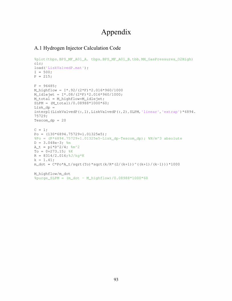
93
Appendix
A.1 Hydrogen Injector Calculation Code %plot(tbps,BPS_MF_A01_A, tbps,BPS_MF_A01_B,tbb,MH_GasPressures_O2High) clc; load('LiskValvedP.mat'); I = 500; P = 215; F = 96485; M_highflow = I*.92/(2*F)*2.016*960/1000 M_idlejet = I*.08/(2*F)*2.016*960/1000; M_total = M_highflow+M_idlejet; SLPM = (M_total)/0.08988*1000*60; Lisk_dp = interp1(LiskValvedP(:,1),LiskValvedP(:,2),SLPM,'linear','extrap')*6894.75729; Tescom_dp = 20 C = 1; Po = (130*6894.75729+1.01325e5); %Po = (P*6894.75729+1.01325e5-Lisk_dp-Tescom_dp); %N/m^3 absolute D = 3.048e-3; %m A_t = pi*D^2/4; %m^2 To = 0+273.15; %K R = 8314/2.016;%J/kg*K k = 1.41; m_dot = C*Po*A_t/sqrt(To)*sqrt(k/R*(2/(k+1))^((k+1)/(k-1)))*1000 M_highflow/m_dot %purge_SLPM = (m_dot - M_highflow)/0.08988*1000*60
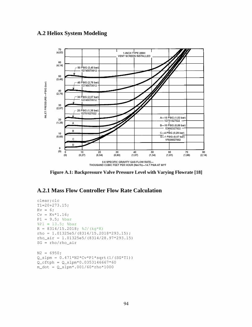
94
A.2 Heliox System Modeling
Figure A.1: Backpressure Valve Pressure Level with Varying Flowrate [18]
A.2.1 Mass Flow Controller Flow Rate Calculation clear;clc T1=20+273.15; Kv = 6; Cv = Kv*1.16; P1 = 9.5; %bar %P1 = 13.5; %bar R = 8314/15.2018; %J/(kg*K) rho = 1.01325e5/(8314/15.2018*293.15); rho_air = 1.01325e5/(8314/28.97*293.15) SG = rho/rho_air N2 = 6950; Q_slpm = 0.471*N2*Cv*P1*sqrt(1/(SG*T1)) Q_cftph = Q_slpm*0.0353146667*60 m_dot = Q_slpm*.001/60*rho*1000

95
A.2.2 Cross Over Tube Model %clear;clc;close all P = 3.4e5; T = 80+273.15; R = 8314/15.2018; %J/(kg*K) %D = .5*0.0254; D = 2*0.0254; E = .0025e-3; A = pi*D^2/4; L = .5588; cp_O2 = (3.626-1.878e-3*T+7.055e-6*T^2-6.764e-9*T^3+2.156e-12*T^4)*8314/32;%J/(kg*K) cp_He = 2.5*8314/4.003;%J/(kg*K) cp = .4*cp_O2+.6*cp_He; gamma = cp/(cp-R); mu_O2 = 2.04e-5; mu_He = 1.94e-5; mu = .4*mu_O2+.6*1.94e-5; M = 0.0001:.0001:1; F = (1-M.^2)./(gamma*M.^2)+(gamma+1)./(2*gamma).*log((gamma+1)*M.^2./(2+(gamma-1)*M.^2)); f = 0:.00001:.1; Re = 2.51./sqrt(f).*(10.^(-.5./sqrt(f))-E/D/3.7).^(-1); f = f(find(Re>=0)); Re = Re(find(Re>=0)); %loglog(Re,f) M1 = 0.01:.01:.999; a = sqrt(gamma*R*T); V = a*M1; rho = P/(R*T); Re_1 = rho*V*D/mu; f1 = interp1(Re,f,Re_1); for(i=1:length(M1)) F1 = 4*f1(i)*L/D; F1_s = (1-M1(i)^2)/(gamma*M1(i)^2)+(gamma+1)/(2*gamma)*log((gamma+1)*M1(i)^2/(2+(gamma-1)*M1(i)^2)); F2_s = F1_s-F1; M2 = interp1(F,M,F2_s); P_ratio(i) = M1(i)/M2*((2+(gamma-1)*M1(i)^2)/(2+(gamma-1)*M2^2))^(1/2); end M1 = M1((not(isnan(P_ratio)))); P_ratio = P_ratio(not(isnan(P_ratio))); m_dot = M1*P*A*sqrt(gamma/(T*R));

96
figure(1) plot(P_ratio.^(-1),m_dot*1000,'r','LineWidth',2) title('\fontsize10\bfCross Over Tube Flowrate (P_i_n_l_e_t = 2.4 barg)'); xlabel('\fontsize10\bfPressure Ratio (P_i_n_l_e_t/P_e_x_i_t)'); ylabel('\fontsize10\bfMass Flowrate [g/s]'); grid on; A.2.3: Heliox Full 2007 System Model
%close all %clear all P_preset = 35 SG = .5247 load air_command_180 Vim = .01095 V_em = .02394 sim Cathode_System_007_2007layout %% figure(1) plot(t,mdot_mfc_A,'r',t,mdot_mfc_B,'b') xlabel('time') ylabel('MFR g/s') legend('MFC A','MFC B') figure(2) plot(t,inlet_P_A,'r',t,inlet_P_B,'b',t,BP,'g') hold on xlabel('time') ylabel('Pressure (psi)') legend('Module A inlet P','Module B inlet P','Back P') save('results_2007_180','t','inlet_P_A','inlet_P_B','BP','mdot_mfc_A','mdot_mfc_B','mdot_exhaust') %V_em = .003491*2 %sim Cathode_System_007_2007layout % % figure(2) % plot(t,inlet_P,'b--',t,BP,'g--') % xlabel('time') % ylabel('Pressure (psi)') % %plot(tbb_cut,PT_A_07_B_cut*14.5,'r-')

97
% %legend('modeled inlet pressure 2007 volumes','modeled back pressure 2007 volumes',... % % 'modeled inlet pressure 2008 volumes','modeled back pressure 2008 volumes,')%,'PT A 07 from OPE') % axis([0 30 20 65])

98
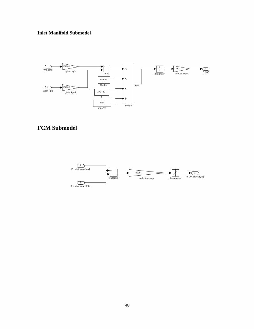
99
Inlet Manifold Submodel
FCM Submodel
1P (psi)
1/1000
g/s to kg/s1
1/1000
g/s to kg/s
Vim
V (m^3)
273+80
T
546.97
Rhelox
-K-
N/m^2 to psi
1s
Integrator
Divide
Add
2Wout (g/s)
1Win (g/s)
dp/dt
1m dot stack (g/s)
80/5
mdot/delta pSubtract Saturation2
P outlet manifold
1P inlet manifold

100
Exhaust Manifold Submodel
A.2.4: Heliox Full 2008 System Model
close all clear all P_preset = 35 SG = .5247 load air_command_180 load Crossover_Tube_Flow_data PR = [wrev(P_ratio_05) P_ratio_05.^-1]; MM = [wrev(M_05) -M_05]; Vim = .01095 V_em = .003491 diam = .5*.0254; %diameter in meters sim Cathode_System_008_2008layout2 %% figure(1) plot(t,mdot_mfc_A,'r',t,mdot_mfc_B,'b') xlabel('time') ylabel('MFR g/s') legend('MFC A','MFC B','exhaust')
1P (psi)
1/1000
g/s to kg/s1
1/1000
g/s to kg/s
V_em
V (m^3)
-C-
T
546.97
Rhelox
.000145
N/m^2 to psi
1s
Integrator
Divide
Add
2Wout (g/s)
1Win (g/s)
dp/dt

101
figure(2) plot(t,inlet_P_A,'r',t,inlet_P_B,'b',t,BP_A,'m',t,BP_B,'k') hold on xlabel('time') ylabel('Pressure (psi)') legend('Module A inlet P','Module B inlet P','Back P A','Back P B') figure(3) plot(t,mdot_exhaust_A,'r',t,mdot_exhaust_B,'b',t,mdot_cross_over,'k') xlabel('time') ylabel('MFR g/s') legend('mdot exhaust A','mdot exhaust B','cross over') %% figure(4) plot(t,mdot_stack_A,'r',t,mdot_exin_A,'k',t,mdot_cross_over,'g',t,mdot_stack_A+mdot_cross_over,'m--') legend('stack A','exaust inlet','cross over','stack A+crossover') %save('results_20082p0','t','inlet_P_A','inlet_P_B','BP_A','BP_B','mdot_mfc_A','mdot_mfc_B','mdot_exhaust_A','mdot_exhaust_B') %V_em = .003491*2 %sim Cathode_System_007_2007layout % % figure(2) % plot(t,inlet_P,'b--',t,BP,'g--') % xlabel('time') % ylabel('Pressure (psi)') % %plot(tbb_cut,PT_A_07_B_cut*14.5,'r-') % %legend('modeled inlet pressure 2007 volumes','modeled back pressure 2007 volumes',... % % 'modeled inlet pressure 2008 volumes','modeled back pressure 2008 volumes,')%,'PT A 07 from OPE') % axis([0 30 20 65])

102

103
Inlet Manifold Submodel
FCM submodel
1P (psi)
1/1000
g/s to kg/s1
1/1000
g/s to kg/s
Vim
V (m^3)
273+80
T
546.97
Rhelox
-K-
N/m^2 to psi
1s
Integrator
Divide
Add
2Wout (g/s)
1Win (g/s)
dp/dt
1m dot stack (g/s)
80/5
mdot/delta pSubtract Saturation2
P outlet manifold
1P inlet manifold

104
Exhaust Manifold Submodel
1P (psi)
1/1000
g/s to kg/s1
1/1000
g/s to kg/s
V_em
V (m^3)
-C-
T
546.97
Rhelox
.000145
N/m^2 to psi
1s
Integrator
Divide
Add
2Wout (g/s)
1Win (g/s)
dp/dt

105
Cross Over Tube submodel

106
A.3: Fuel Cell Empirical Model Code
addpath('data'); clc;clear;%close all; data1 = load('June27Run2.txt'); data2 = load('June26Run1.txt'); data3 = load('June23Run1.txt'); data4 = load('June19Run1.txt'); data5 = load('June18Run1.txt'); data6 = load('June29Run1a.txt'); data7 = load('June29Run1b.txt'); data8 = load('June29Run2a.txt'); data9 = load('June29Run2b.txt'); data10 = load('June29Run2c.txt'); data11 = load('August22Run1a.txt'); data12 = load('August22Run1b.txt'); data13 = load('August22Run1c.txt'); data14 = load('August22Run1d.txt'); data15 = load('August22Run2a.txt'); data16 = load('August22Run2b.txt'); data17 = load('August22Run2c.txt'); data18 = load('August22Run2d.txt'); data19 = load('August22Run3a.txt'); data20 = load('August22Run3b.txt'); data21 = load('August22Run3c.txt'); data22 = load('August22Run3d.txt'); data23 = load('August23Run1a.txt'); data24 = load('August23Run1b.txt'); data25 = load('August23Run1c.txt'); data26 = load('August23Run1d.txt'); data = [data1 data2 data3 data6 data7 data8 data9 data10 data11 data12 data13 data14 data15 data16 data17 data18 data19 data20 data21 data22 data23 data24 data25 data26];

107
%data = [data1;data2;data3;data6;data7;data8;data9;data10;data11;data12;data13;data14;data15;data16;data17;data18]; %data = [data1;data2;data3;data6;data7;data8;data9;data10]; load('FC_polar.mat') %% % x = find(data(:,2)>400); % data = data(x,:) %% %Raw Data t = data(:,1); CT_F01_A = data(:,2); CT_F01_B = data(:,3); PT_A07_A = data(:,4); PT_H03_A = data(:,5); PT_H03_B = data(:,6); TT_A09_A = data(:,7); TT_A09_B = data(:,8); TT_D02_A = data(:,9); VE_STA = data(:,10); VE_STB = data(:,11); VE_STC = data(:,12); VE_STD = data(:,13); %% %Parameters mm_helox = 15.201; %g/mol mole_frac = .4;%.4*15.201/31.9880; %R_bar = 8.314; %kJ/kmol*K %R_O2 = R_bar/mm_helox; %% %Data Manipulation V = (VE_STA + VE_STB); T = TT_D02_A+273.15; I = CT_F01_A; P_O2 = mole_frac.*PT_A07_A; %partial pressure of O2 %% %Nerst Equation Nernst = 1.229 - 8.5e-4 * (T-298.15) + 4.3085e-5*T .* (log(PT_H03_A) + .5.*log(P_O2)); E0 = Nernst * 960; %% x = find(I>250); Vact_terms = [ones(length(I),1),T]*960; Vohm_terms = [I, I.*T, I.*I]*960; b = E0(x) - V(x); A = [Vact_terms(x,:) Vohm_terms(x,:)]; c1 = inv(A'*A)*A'*b; ohmic_c = c1(3:5) Vohm = Vohm_terms*c1(3:5); Vact = Vact_terms*c1(1:2); V_theo = E0 - Vact-Vohm;

108
C_O2 = P_O2./(5.08e6.*exp(-498./T)); Vact_terms = [ones(length(I),1), T, T.*log(C_O2), T.*log(I)]*960; b = E0 - V- Vohm; A = [Vact_terms]; c2 = inv(A'*A)*A'*b; Vact = A*c2; V_theo = E0 - Vact - Vohm; activation_c = c2 %% % figure(1) % plot(t,V,'b+',t,V_theo,'g+') % title('Experimental Data Fit') % xlabel('Time [s]'); % ylabel('Voltage [V]'); % legend('Experimental','Theorectical','Location','SouthEast'); % grid on; %% figure(2) title('Experimental Data Fit') plot(T-273.15,V, 'b+',T-273.15,V_theo,'g+'); xlabel('Temperature [C]'); ylabel('Voltage [V]'); legend('Experimental','Theorectical','Location','SouthEast'); grid on; %% % figure(3) % plot(I,V,'b+',I,V_theo,'g+',FC_I/2,FC_V/.97,'rO'); % % grid on; %% % figure(4);plot(... % I,Vact,'bx',... % I,Vohm,'b^'); % grid on; %% figure(5) x1 = find(T>273.15 & T<=20+273.15); x2 = find(T>20+273.15 & T<=40+273.15); x3 = find(T>40+273.15 & T<=60+273.15); x4 = find(T>60+273.15 & T<=80+273.15); x5 = find(T>80+273.15); hold on; % plot(I(x1),V(x1),'b+',I(x1),V_theo(x1),'b^'); % plot(I(x2),V(x2),'c+',I(x2),V_theo(x2),'c^'); % plot(I(x3),V(x3),'g+',I(x3),V_theo(x3),'g^'); % plot(I(x4),V(x4),'r+',I(x4),V_theo(x4),'r^'); % plot(I(x5),V(x5),'m+',I(x5),V_theo(x5),'m^'); plot(I(x1),V(x1),'b+'); plot(I(x2),V(x2),'c+'); plot(I(x3),V(x3),'g+'); plot(I(x4),V(x4),'r+'); plot(I(x5),V(x5),'m+'); title('\fontsize10\bfExperimental Data Fit: Polarization Curve'); xlabel('\fontsize10\bfCurrent [amps]'); ylabel('\fontsize10\bfVoltage [Volts]'); legend('20^oC','40^oC','60^oC','80^oC');
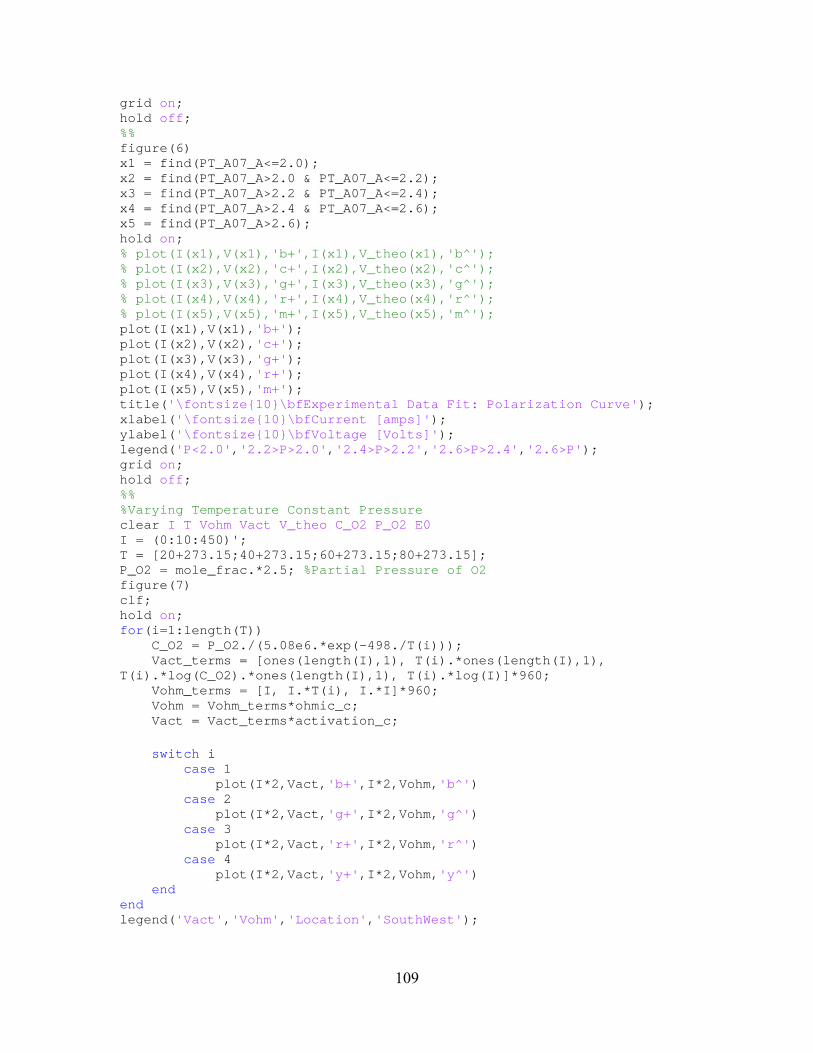
109
grid on; hold off; %% figure(6) x1 = find(PT_A07_A<=2.0); x2 = find(PT_A07_A>2.0 & PT_A07_A<=2.2); x3 = find(PT_A07_A>2.2 & PT_A07_A<=2.4); x4 = find(PT_A07_A>2.4 & PT_A07_A<=2.6); x5 = find(PT_A07_A>2.6); hold on; % plot(I(x1),V(x1),'b+',I(x1),V_theo(x1),'b^'); % plot(I(x2),V(x2),'c+',I(x2),V_theo(x2),'c^'); % plot(I(x3),V(x3),'g+',I(x3),V_theo(x3),'g^'); % plot(I(x4),V(x4),'r+',I(x4),V_theo(x4),'r^'); % plot(I(x5),V(x5),'m+',I(x5),V_theo(x5),'m^'); plot(I(x1),V(x1),'b+'); plot(I(x2),V(x2),'c+'); plot(I(x3),V(x3),'g+'); plot(I(x4),V(x4),'r+'); plot(I(x5),V(x5),'m+'); title('\fontsize10\bfExperimental Data Fit: Polarization Curve'); xlabel('\fontsize10\bfCurrent [amps]'); ylabel('\fontsize10\bfVoltage [Volts]'); legend('P<2.0','2.2>P>2.0','2.4>P>2.2','2.6>P>2.4','2.6>P'); grid on; hold off; %% %Varying Temperature Constant Pressure clear I T Vohm Vact V_theo C_O2 P_O2 E0 I = (0:10:450)'; T = [20+273.15;40+273.15;60+273.15;80+273.15]; P_O2 = mole_frac.*2.5; %Partial Pressure of O2 figure(7) clf; hold on; for(i=1:length(T)) C_O2 = P_O2./(5.08e6.*exp(-498./T(i))); Vact_terms = [ones(length(I),1), T(i).*ones(length(I),1), T(i).*log(C_O2).*ones(length(I),1), T(i).*log(I)]*960; Vohm_terms = [I, I.*T(i), I.*I]*960; Vohm = Vohm_terms*ohmic_c; Vact = Vact_terms*activation_c; switch i case 1 plot(I*2,Vact,'b+',I*2,Vohm,'b^') case 2 plot(I*2,Vact,'g+',I*2,Vohm,'g^') case 3 plot(I*2,Vact,'r+',I*2,Vohm,'r^') case 4 plot(I*2,Vact,'y+',I*2,Vohm,'y^') end end legend('Vact','Vohm','Location','SouthWest');

110
legend('V_a_c_t at 20^oC','V_o_h_m at 20^oC','V_a_c_t at 40^oC','V_o_h_m at 40^oC','V_a_c_t at 60^oC','V_o_h_m at 60^oC','V_a_c_t at 80^oC','V_o_h_m at 80^oC','Location','EastOutside'); xlabel('\fontsize10\bfCurrent [Amps]'); ylabel('\fontsize10\bfVoltage Loss [V]'); grid on; hold off; %% figure(8) clf; hold on; for(i=1:length(T)) Nernst = 1.229 - 8.5e-4 * (T(i)-298.15) + 4.3085e-5*T(i) .* (log(3) + .5.*log(P_O2)); E0 = Nernst * 960; C_O2 = P_O2./(5.08e6.*exp(-498./T(i))); Vact_terms = [ones(length(I),1), T(i).*ones(length(I),1), T(i).*log(C_O2).*ones(length(I),1), T(i).*log(I)]*960; Vohm_terms = [I, I.*T(i), I.*I]*960; Vohm = Vohm_terms*ohmic_c; Vact = Vact_terms*activation_c; switch i case 1 plot(I*2,E0-Vact-Vohm,'b+') case 2 plot(I*2,E0-Vact-Vohm,'g+') case 3 plot(I*2,E0-Vact-Vohm,'r+') case 4 plot(I*2,E0-Vact-Vohm,'m+') end end %plot(FC_I/2,FC_V/.97,'rO'); title('\fontsize10\bfBB2 Polarization Curve'); xlabel('\fontsize10\bfCurrent [amps]'); ylabel('\fontsize10\bfVoltage [Volts]'); grid on; legend('20^oC','40^oC','60^oC','80^oC'); hold off; %% figure(9) clf; hold on; for(i=1:length(T)) Nernst = 1.229 - 8.5e-4 * (T(i)-298.15) + 4.3085e-5*T(i) .* (log(3) + .5.*log(P_O2)); E0 = Nernst * 960; C_O2 = P_O2./(5.08e6.*exp(-498./T(i))); Vact_terms = [ones(length(I),1), T(i).*ones(length(I),1), T(i).*log(C_O2).*ones(length(I),1), T(i).*log(I)]*960; Vohm_terms = [I, I.*T(i), I.*I]*960; Vohm = Vohm_terms*ohmic_c; Vact = Vact_terms*activation_c; yunit = 1000; ylabel('\fontsize10\bfPower [kW]') % yunit = 746; ylabel('\fontsize10\bfPower [HP]') switch i case 1

111
plot(I*2,(E0-Vact-Vohm).*I*2/yunit,'b+') case 2 plot(I*2,(E0-Vact-Vohm).*I*2/yunit,'g+') case 3 plot(I*2,(E0-Vact-Vohm).*I*2/yunit,'r+') case 4 plot(I*2,(E0-Vact-Vohm).*I*2/yunit,'m+') end end title('\fontsize10\bfBB2 Power Curve'); xlabel('\fontsize10\bfCurrent [amps]'); grid on; legend('20^oC','40^oC','60^oC','80^oC','Location','SE'); hold off; %% figure(10) clf; hold on; clear I T T = (60 + 273.15); I = (0:500/7:500)'; Nernst = 1.229 - 8.5e-4 * (T-298.15) + 4.3085e-5*T .* (log(3) + .5.*log(P_O2)); E0 = Nernst * 960; C_O2 = P_O2./(5.08e6.*exp(-498/T)); Vact_terms = [ones(length(I),1), T*ones(length(I),1), T*log(C_O2).*ones(length(I),1), T*log(I)]*960; Vohm_terms = [I, I*T, I.*I]*960; Vohm = Vohm_terms*ohmic_c; Vact = Vact_terms*activation_c; P_curve_I = 2.*I; P_curve_V = E0-Vact-Vohm; P_curve_V(1) = 960; plot(P_curve_I,P_curve_V,'b+') title('Polarization Curve'); xlabel('Current [amps]'); ylabel('Voltage [Volts]'); grid on; hold off; %% %Varying Temperature Constant Pressure figure(11) I = (0:10:450)'; T = [80+273.15]; ohmic_c2007 = [6.417e-4 -1.813e-7 1.653e-8]'; activation_c2007 = [.8193 -3.186e-3 -7.608e-5 1.264e-4]'; clf; hold on; Nernst = 1.229 - 8.5e-4 * (T-298.15) + 4.3085e-5*T.*(log(3)+ .5.*log(P_O2)); E0 = Nernst * 960; C_O2 = P_O2./(5.08e6.*exp(-498./T)); Vact_terms = [ones(length(I),1), T.*ones(length(I),1), T.*log(C_O2).*ones(length(I),1), T.*log(I)]*960;

112
Vohm_terms = [I, I.*T, I.*I]*960; Vohm = Vohm_terms*ohmic_c; Vact = Vact_terms*activation_c; V_2008 = E0-Vact-Vohm; plot(I*2,V_2008,'b','LineWidth',2) Vohm = Vohm_terms*ohmic_c2007; Vact = Vact_terms*activation_c2007; V_2007 = E0-Vact-Vohm; plot(I*2,V_2007,'g','LineWidth',2) %plot(FC_I/2,FC_V/.97,'rO'); title('\fontsize10\bfBB2 Polarization Curve'); xlabel('\fontsize10\bfCurrent [amps]'); ylabel('\fontsize10\bfVoltage [Volts]'); grid on; legend('2008','2007'); hold off; figure(12) plot(I*2,I.*2.*V_2008/1000,'b',I*2,I.*2.*V_2007/1000,'g','LineWidth',2) title('\fontsize10\bfBB2 Polarization Curve'); xlabel('\fontsize10\bfCurrent [amps]'); ylabel('\fontsize10\bfPower [kW]'); grid on; legend('2008','2007','Location','SE'); hold off;