development and field testing of a new intelligent

DEVELOPMENT AND FIELD TESTING OF A NEW INTELLIGENT SEQUENCING BATCH REACTOR (iSBR) CONTROL SYSTEM

Andrew W. Fairey*, Andrew Shaw**, October McConnell** and John Cook*

*Charleston Water System P.O. Box B, 103 St.Philip Street

Charleston, SC 29402

** Black & Veatch

ABSTRACT The Daniel Island WWTP serves an area that is experiencing phenomenal growth. The Sequencing Batch Reactors (SBR) that provide secondary treatment at the plant are rapidly approaching their design capacity and so the Charleston Water System commissioned Black & Veatch to investigate options to optimize the treatment capacity of the SBRs beyond their existing design capacity. The plant optimization used an intelligent control approach termed the “intelligent” SBR or “iSBR”. The iSBR control approach measures the oxygen uptake rate (OUR) of the mixed liquor to determine when the SBR has completed treatment, indicated by a sudden decrease in the OUR as the activated sludge reaches an endogenous state. The iSBR control was tested in two steps. Firstly, a dynamic process model of the plant was used to prove iSBR control approaches based on OUR, dissolved oxygen (DO) and rate of change of DO (“dO/dt”). Secondly, a 5-day full-scale trial was carried out on one of the SBRs at Daniel Island. The full-scale trial was successful and so the control was left in operation after the trial period was over. This is the first time the iSBR control approach has been used successfully in a full-scale application. The iSBR control system in conjunction with the addition of extra aeration capacity enabled the plant to increase its design rating by 50%. Addition of an influent equalization tank will enable the plant to increase its design still further to effectively double the plant capacity. KEYWORDS SBR, control, DO, respiration rate, aeration BACKGROUND Wastewater is fed to the Daniel Island plant from several pump stations on the island. It then passes through a manually cleaned convex-sieve screen before entering the SBRs without primary treatment. The two SBRs at Daniel Island WWTP were originally designed to treat a total flow of 0.5 mgd and their design criteria are summarized in Table 1. The fill sequence is conducted for each of the two SBRs alternately: as one SBR fills and carries out treatment, the other is in the final stages of aeration, settling, and decanting. Figure 1 is a photograph of one of the SBRs during an aeration phase. Decant water from the SBRs is passed to an equalization

7018

WEFTEC®.06

Copyright 2006 Water Environment Foundation. All Rights Reserved©

basin via gravity. From the equalization basin, the flow is pumped to disc filters and then flows on to UV disinfection before being pumped to the discharge point.

Figure 1: Daniel Island SBR During Aerate Phase

Table 1 SBR Design Criteria

Number of Treatment Cycles per Day 5 Cycle Duration (hr) 4.8 Maximum Food/Mass (F/M) Ratio (lb BOD5 / lb MLSS-day) 0.076 Maximum MLSS Concentration (mg/L @ Min. Water Depth) 4500 Hydraulic Retention Time (days @ Avg. Water Depth) 0.934 Minimum Solids Retention Time (days) 15.2 Actual Oxygen Required (lbs/day) 2070 Carbonaceous Demand Basis (lbs O2 / lb BOD5) 1.25 Nitrogenous Demand Basis (lbs O2 / lb TKN) 4.6

The plant currently has a permit to discharge up to 0.5 mgd of treated effluent to a small unnamed tributary to the Cooper River. A revised permit was developed - and a draft has been issued by the South Carolina Department of Health and Environmental Control (SCDHEC) - that will allow the plant to eventually discharge up to 4 mgd through a new outfall directly to the Cooper River, as the treatment capacity is increased in various stages. The new permit includes the parameter “Ultimate Oxygen Demand” (UOD), which becomes the limiting factor when analyzing the SBR effluent at flows above 1 mgd as opposed to the current limiting parameters

7019

WEFTEC®.06


of BOD, TSS, and seasonal ammonia. Table 2 summarizes the effluent design parameters used by Aqua-Aerobic Systems, Inc. (line 1) for the 0.5 mgd rated SBRs and the chronological list of current (line 2) and future (lines 3 -5) outfall permits to be issued to the Daniel Island WWTP.

Table 2: Effluent Design and Permit Information

Flow BOD TSS Amm-Nit UOD1

Monthly Averages Mar – Oct Nov – Feb Mar – Oct

Nov – Feb

mgd mg/L ppd mg/L ppd mg/L ppd mg/L ppd ppd ppd

1. Effluent Design 0.5 10 42 10 42 1.0 4.2 1.0 4.2 -- --

2. Current Permit2 0.5 5 21 30 125 0.87 3.6 1.94 8.1 -- --

3. Future Permit2 1.0 16.1 134 30 250 5.28 44.0 7 58.4 402.7 468.2

4. Future Permit2 2.0 16.1 269 30 500 5.28 88.1 7 116.8 402.7 936.4

5. Maximum Permit2 4.0 8.05 269 30 1001 2.64 88.1 7 233.5 402.7 1872.8

Notes: 1 - UOD = Ultimate Oxygen Demand UOD pounds per day (ppd) = [1.5 x BOD5 (mg/L) + 4.57 x NH3-N (mg/L)] x Flow (mgd) x 8.34

2 - Permits shown are average monthly values. The permits also include a weekly average limit for loads and concentrations of 1.5 times the monthly limit. Weekly flow limit is the same as the monthly limit. Daniel Island is an area undergoing rapid development, which is causing the plant influent flows to increase dramatically. Figure 2 is a plot of the monthly average influent flow to the plant showing a significant flow increase from less than 0.1 mgd in 2000 to almost the 0.5 mgd design (and current permit) limit by the beginning of 2006. A linear trend line is shown in black and a quadratic curve trend line in blue. The latter trend has a better fit with the data and is likely a better indicator of future flow trends. The rapid increase in flows coupled with difficulties in getting access to easement to put in the new outfall necessary for the future permit caused Charleston Water System to look to optimize and rerate the current plant in order to “buy time” to provide additional capacity. The optimization steps described later in this paper were able to increase the plant capacity to 0.75 mgd with the addition of extra aeration and additional UV units, or to 1.0 mgd with an influent equalization tank. The dotted lines on Figure 2 show the dates by which these new flow limits would be reached. It can be seen that increasing the current plant capacity to 0.75 mgd enables the plant to handle future flows for an extra 2 years: a 1.0 mgd capacity will accommodate flows for a further 1½ years beyond that.

7020

WEFTEC®.06


Daniel Island Average Monthly Flow (2000 - Present)Through February 2006

R2 = 0.9415

R2 = 0.9719

0.000

0.100

0.200

0.300

0.400

0.500

0.600

0.700

0.800

0.900

1.000

Jan-0

0Ju

l-00

Jan-0

1Ju

l-01

Jan-0

2Ju

l-02

Jan-0

3Ju

l-03

Jan-0

4Ju

l-04

Jan-0

5Ju

l-05

Jan-0

6Ju

l-06

Jan-0

7Ju

l-07

Jan-0

8Ju

l-08

Jan-0

9Ju

l-09

Jan-1

0Ju

l-10

Jan-1

1Ju

l-11

Jan-1

2

Date

Avg

. Mon

thly

Flo

w (M

GD

)

NPDES PERMIT LIMIT (Current Plant Capacity): 0.50 MGD

PERMIT LIMIT (w/Aeration & UV): 0.75 MGD

PERMIT LIMIT (w/EQ Tank): 1.0 MGD

@0.75 MGDFebruary 2008

@0.75 MGDAugust 2010

@0.5 MGDDecember 2007

@0.5 MGDMarch 2006

@1.0 MGDAugust 2009

Figure 2: Daniel Island Flow Projections (Data from Jan 2000 to Feb 2006)

A further problem facing the Daniel Island WWTP is the hurricane season that can cause a rapid influx of rain which affects the flow and loads entering the plant. For the period from July 2004 to October 2004 (a particularly active hurricane season for the area with no less than 5 hurricanes passing through), the effluent ammonia was compared to the daily rainfall and daily flow in Figure 3. It was determined that the increase in rainfall has little impact on the effluent ammonia concentration. The plant saw a significant increase in the daily flow caused by 4 inches of rain from Hurricane Gaston, but this did not impact the plant’s ability to maintain a low effluent ammonia concentration. (Similarly, the increased rainfall did not have a great impact on any of the other effluent parameters not shown). A slight increase in the effluent ammonia concentration to 0.37 mg/L can be seen when Hurricane Jeanne passed through, but this was still well below the peak day effluent limit of 1.31 mg/L and even the monthly average limit of 0.87 mg/L (the corresponding ammonia load was 1.33ppd, which is also significantly below the permit limits). During September of 2004, the average influent flow rate was 0.405 mgd, which exceeds the 80% design flow. It can be seen that the rainfall associated with hurricanes has a significant impact on the monthly flows seen at the plant.

7021

WEFTEC®.06


Daniel Island Flow vs. Daily Rainfall

0.00

0.10

0.20

0.30

0.40

0.50

0.60

0.70

Date

Avg

. Dai

ly F

low

(MG

D)/

Efflu

ent A

mm

onia

(mg/

L)

0.00

0.50

1.00

1.50

2.00

2.50

3.00

3.50

4.00

4.50

Dai

ly R

ainf

all (

in)

ADFEffluent AmmoniaDaily Rainfall

Hurricane Alex

Hurricane Charlie

Hurricane Gaston

Hurricane Ivan

Hurricane Jeanne

Figure 3: Plant Average Daily Flow (ADF), Rainfall and Effluent Ammonia (dotted line) through the busy 2004 Hurricane Season

THE iSBR CONTROL APPROACH The term “iSBR” was first coined by Dr John Watts the then managing director of Minworth Systems Limited, around the turn of the century, and the concept was first presented at WEFTEC in Atlanta in 2001 (Shaw et al, 2001). Subsequently, the basis for the iSBR concept, which is to use respirometric measurements to determine when treatment is complete, was further described in several papers, presentations and workshops (Shaw and Watts, 2002; Barnard et al, 2003; Shaw, 2003). Several other authors have published papers describing the use of various parameters to control SBRs, including respirometric control, DO, ORP and pH. Some of the more notable work includes: Yoong et al (2000), Cohen, et al (2003); Cho et al (2001), Andreotta et al (2001) and Demoulin et al (1997). Most of these papers are based on pilot and bench-scale test work, with the notable exception of Demoulin et al who used a combination of ORP and DO to control the full-scale cyclical activated sludge technology (CAST) system at the Großarl WWTP. Figure 4 shows a typical output (respirogram) from a batch respirometry test for a nitrifying activated sludge, showing the change in oxygen uptake rate (OUR) versus time for the test batch. The respirogram in Figure 4 is labeled to show the oxygen demand associated with different substrates present in the activated sludge at the start of treatment. The peak at the start of the respirogram is caused by the presence of readily-biodegradable carbon substrate and the gradual

7022

WEFTEC®.06


slope is caused by the hydrolysis and oxidation of slowly-degradable material. Beneath these two sections is the oxygen demand for nitrification which is exerted at a relatively constant rate until all the ammonia is used up and the respiration rate drops down to the endogenous rate. At this point all of the carbon substrate is either used up or absorbed into the floc and all of the ammonia has been oxidized. Treatment is effectively complete.

Readily Biodegradable Carbon Substrate

Slowly Biodegradable Carbon Substrate

Nitrification

Endogenous

Time Figure 4: Typical Respirogram for a Nitrifying Activated Sludge

It is the distinct drop in respiration rate at the point at which all of the ammonia is used up – termed the “nitrification shoulder” - that can be used to detect the point at which treatment is complete in an SBR. The respiration rate observed in an SBR is similar to that seen in a batch-fed respirometer but it is slightly different because filling and treatment occur concurrently at the start of the SBR treatment cycles. Figure 5 shows the respirogram for an example SBR system modeled using the GPS-X process simulator (in blue). On the same graph are shown the ammonia (green) and nitrate (red) concentrations for the same time period. The circled area is the point at which the ammonia is completely oxidized and treatment is complete. It can be seen that the OUR has the characteristic nitrification shoulder at this point. It can also be seen that in this example, treatment is complete at 3 hours, even though the aerate phase continues for another 1½ hours to 4½ hours. The time from 3 hours to 4½ hours is a period where no useful treatment occurs and air is effectively wasted. If this period is too long, it can also promote the growth of low F:M filaments.

7023

WEFTEC®.06


Figure 5: Example SBR Respirogram

The iSBR control works by detecting the nitrification shoulder in the OUR curve and ceasing aeration at this point. The SBR can then go into an extended settle period or the settle and decant phases advanced to allow the total cycle time to be shortened and more cycles to be completed in a day. Potential benefits of the iSBR control include the following:

1. Energy savings by stopping treatment at the endogenous point 2. Increased viability of the nitrifying biomass by reducing aerobic endogenous treatment. 3. Shorter aerate times, facilitating more cycles per day (increased hydraulic capacity), or

longer settle times. 4. Reduced potential for filament growth. Potentially better settling sludge. 5. Reduced nitrate concentrations as biomass is aerated for a shorter proportion of the

treatment time, facilitating more anoxic time. The main benefit of interest for Daniel Island is number 3 – reducing the aerate time. This could be used to increase the hydraulic capacity of the SBRs but, more usefully, it allows them to have longer settle times. Historically, the plant SVI is very variable and can reach as high as 200 mL/g. A capacity analysis of the plant indicated that the SBRs could just about cope with SVIs this high but a marginal deterioration in settling characteristics could cause the settling to become critical. The iSBR control could be used to extend the settle time slightly to ensure that it is not critical. An extra 10 or 20 minutes in the settling time is of more benefit than decreasing the overall cycle time by the same amount. In addition to this, benefit number 4 – reduced filament growth - should help prevent the SVIs from rising to historic highs.

Treatment Complete

7024

WEFTEC®.06


PROCESS MODELING – CAPACITY ASSESSMENT A dynamic process model of one of the SBRs was developed as part of the plant capacity evaluation using the Hydromantis GPS-X simulator (Version 4.1). GPS-X contains an SBR model that can be used to dynamically simulate the operation of the SBRs at Daniel Island. The model includes kinetic formulas to simulate the biological activity of the activated sludge in the basins, using a modified version of the IWA activated sludge model, ASM1 (termed the “Mantis” kinetics in GPS-X). These kinetic expressions describe the transformation of carbon and nitrogen compounds under aerobic and anoxic conditions. The kinetics selected for the Daniel Island model do not include expressions for phosphorus compounds as phosphorus removal is not a concern at present. In addition to modeling, biological processes, the SBR model includes salient hydraulic expressions to model variation in the liquid volume as the SBR fills and empties (including an “overflow” line). Finally, the SBR model also includes a model to describe the way in which the sludge settles during the settling phase of operation. The SBR model requires the user to define the operation of the SBR phases in one of three ways. In the “simple” operating mode, used in this study, the user simply defines the overall cycle time and the timings for individual phases (fill, fill & aerate, aerate, settle, decant and desludge) which occur separately in sequential order. Alternatively, the model can be operated in an “advanced” mode that allows the user to specify start and stop times for each phase independently. This allows the user to specify operating phases that overlap or occur concurrently. The final operating mode – “manual” – can be used to allow the user to manually control the different operating phases. Further details of the SBR model can be found in the GPS-X Technical Reference Manual (2003). An initial capacity analysis was carried out using the simple operating mode to describe the plant operation. This mode can be used to fully define the operation of the Daniel Island SBRs with the minor exception of the wasting, or “desludging.” In the simple SBR model operation, the desludge phase occurs separately after the decant has finished whereas the Daniel Island SBRs desludge in the final few minutes of the decant, occurring concurrently with the decant. This slight difference in the operation was accounted for in the model simulations by increasing the decant flow slightly; in proportion to the additional decant time that would occur in the real plant. Figure 6 is the GPS-X model layout for the Daniel Island plant. It can be seen that the model includes just one of the SBRs (SBR #1) but that the influent flow is split two ways (at the blue triangle splitter). This was done to simplify the model, enabling it to run faster and be more stable. The second SBR was not included, but would operate identically to the first SBR in the simulations and so it is not necessary to include it for the current study. The flow split was set up on a timer synchronized to send flow to SBR #1 when it was due to be filled. An equalization tank (POST-EQ) is included in the flow schematic and was set up with the flow passing straight through it for the initial analysis. The operation of the EQ tank pumps was not modeled in the first part of the capacity analysis – looking at normal daily flows – but was used in a modified version of the model to carry out a storm flow analysis.

7025

WEFTEC®.06


Figure 6: iSBR Model in GPS-X

The most important aspect of modeling any wastewater treatment facility is having an accurate picture of the influent characteristics. For most process simulations, steady-state calculations (i.e. all values fixed over time) are carried out using daily or monthly averaged influent data. However, because the SBR process is by definition a batch process it cannot be modeled using average daily or monthly values at a steady-state because the process does not operate at a steady state. In order to accurately model the process a dynamic simulation – where all variables change with time - must be carried out. This required extensive diurnal sampling of the influent BOD, TSS and TKN to be carried out by Charleston Water System staff. Figure 7 shows the diurnal concentrations expressed as a fraction of the average concentration that were calculated from these samples. In addition to the diurnal sampling, several other samples were taken in order to develop a more detailed influent characterization that was used in the model.

0.00

0.20

0.40

0.60

0.80

1.00

1.20

1.40

0:00 2:00 4:00 6:00 8:00 10:00 12:00 14:00 16:00 18:00 20:00 22:00

Time (hr)

Diu

rnal

Fra

ctio

n

BODTSSTKN

Figure 7: Influent Diurnal Concentrations

7026

WEFTEC®.06


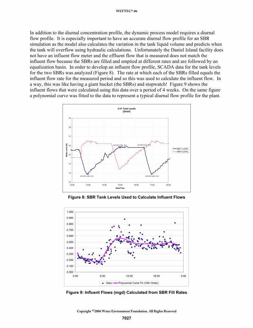
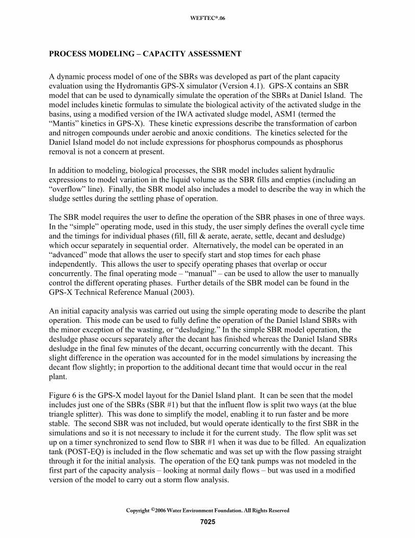
In addition to the diurnal concentration profile, the dynamic process model requires a diurnal flow profile. It is especially important to have an accurate diurnal flow profile for an SBR simulation as the model also calculates the variation in the tank liquid volume and predicts when the tank will overflow using hydraulic calculations. Unfortunately the Daniel Island facility does not have an influent flow meter and the effluent flow that is measured does not match the influent flow because the SBRs are filled and emptied at different rates and are followed by an equalization basin. In order to develop an influent flow profile, SCADA data for the tank levels for the two SBRs was analyzed (Figure 8). The rate at which each of the SBRs filled equals the influent flow rate for the measured period and so this was used to calculate the influent flow. In a way, this was like having a giant bucket (the SBRs) and stopwatch! Figure 9 shows the influent flows that were calculated using this data over a period of 4 weeks. On the same figure a polynomial curve was fitted to the data to represent a typical diurnal flow profile for the plant.

2-21 Tank Levels(Detail)

2/21/05 12:55, 12.9

2/21/05 14:59, 15.8 2/21/05 16:29, 15.8

2/21/05 16:59, 12.9

12

13

14

15

16

17

18

19

12:00 13:00 14:00 15:00 16:00 17:00 18:00

Date/Time

Wat

er L

evel

(ft)

SBR 1 LEVELSBR 2 LEVEL

Figure 8: SBR Tank Levels Used to Calculate Influent Flows

0.000

0.100

0.200

0.300

0.400

0.500

0.600

0.700

0.800

0.900

1.000

0:00 6:00 12:00 18:00 0:00

Data Polynomial Curve Fit (10th Order)

Figure 9: Influent Flows (mgd) Calculated from SBR Fill Rates

7027

WEFTEC®.06


Several dynamic model runs were carried out to determine the maximum capacity of the SBR model. In each case, three criteria were used to assess the model performance and adjustments were made to flows and operating times to keep the SBR within these criteria:

1. Hydraulic capacity – the SBR should not overflow (max liquid height = 19.3 ft). Figure 10 shows how the height of liquid varied based on the influent flow to it and the batch operation for one of the model simulations.

2. Biological capacity – the effluent ammonia load must be less than the target load (3.6 ppd)

3. Settling – the SBR effluent should not contain excessive solids. The settling model does not produce a totally accurate prediction of effluent TSS – tending to overestimate effluent solids – but can be used to give an indication of the SBR reaching its limit for handling solids or being in danger of losing its blanket. For this purpose, a target effluent TSS of 20 mg/L was selected as an acceptable maximum (note also that the SBR is followed by a tertiary filter).

In addition to the constraints listed above, the maximum MLSS was maintained between 4000 and 4500 mg/L (design value max is 4500 mg/L) and the phase timings were set up to ensure that filling and aeration were correctly synchronized between the two SBRs.

Height & Flow

1011121314151617181920

0.0 0.5 1.0 1.5 2.0 2.5 3.0Time (days)

Heig

ht (f

t)

0.000.100.200.300.400.500.600.700.800.901.00

Flow

(mgd

)

Height Max Height

Minimum Height SBR1 Flow

Figure 10: SBR Liquid Height and Flow for a 3-day, 0.7 mgd Simulation

Based on the modeling analysis it was found that the SBRs could adequately treat up to 0.75mgd of flow on an average monthly basis, provided that additional blowers were installed. In addition to this, it was found that if the influent flow was equalized, the plant could be pushed further to treat up to 1.0 mgd of flow. In order to achieve these maximum capacities it was recognized that the SBR control must be optimized and so the iSBR control was proposed to facilitate this.

7028

WEFTEC®.06


DEVELOPMENT OF CONTROL ALGORITHMS Development of the iSBR control algorithms was carried out using data produced from the model used for the capacity assessment. Control algorithms based on one of three different parameters were developed: OUR, DO and the rate of change of DO (termed the DO derivative or “dO/dt”). Figure 11 shows the way in which the OUR (in red) and DO (blue) varied as the SBR model goes through its 5 cycles per day for a 2 day period. The SBR has a fixed speed blower and so as the OUR decreases, the residual DO increases. Figure 12 shows the OUR profile for the 5th cycle in more detail, as well as the average basin ammonia concentration. Figure 12 clearly shows the characteristic “shoulder” at the point at which the ammonia is depleted and drops down to near zero, indicating nitrification treatment is complete. In this particular example, this occurs very soon after filling, at a time of about 0.903 days (approximately 9:40 pm), and endogenation occurs for almost all of the 35 minute aerate cycle. Figure 13 shows the OUR profile for the same cycle, but this time it is superimposed with the DO profile for the same time period. The 0.903 time at which the biomass activity becomes endogenous is indicated on both curves. In addition, the start (0.900 days) and end (0.925 days) of the aerate phase are labeled on the OUR curve.

0

10

20

30

40

50

60

70

80

90

100

0.00 0.25 0.50 0.75 1.00 1.25 1.50 1.75 2.00

Time (days)

OU

R (m

g/L/

hr)

0

1

2

3

4

5

6

7

8

9

10

DO

(mg/

L)

OUR (Actual) Dissolved Oxygen

Figure 11: OUR and Dissolved Oxygen Profile for 0.7 mgd AA Model

7029

WEFTEC®.06


Anoxic Fill Aerate & Fill Aerate Settle Decant

Was

te

0.9030

10

20

30

40

50

60

70

80

90

100

0.80 0.82 0.84 0.86 0.88 0.90 0.92 0.94 0.96 0.98 1.00

Time (days)

OU

R (m

g/L/

hr)

0

1

2

3

4

5

6

7

8

9

10

Am

mon

ia (m

g/L)

OUR (Actual) Avg Basin Ammonia

Figure 12: OUR and Ammonia Profile for Cycle 5

0.900

0.925

Anoxic Fill Aerate & Fill Aerate Settle Decant

Was

te

0.903

0

10

20

30

40

50

60

70

80

90

100

0.80 0.82 0.84 0.86 0.88 0.90 0.92 0.94 0.96 0.98 1.00

Time (days)

OU

R (m

g/L/

hr)

0

1

2

3

4

5

6

7

8

9

10

DO

(mg/

L)

OUR (Actual) Dissolved Oxygen

Figure 13: OUR and DO Profile for Cycle 5

Using the portion of these curves in the aerate phase, one of two approaches could be used to detect when the biomass has become endogenous:

1. If the OUR drops below a certain setpoint then it is endogenous. 2. If the DO rises above a certain setpoint then it is also endogenous.

7030

WEFTEC®.06


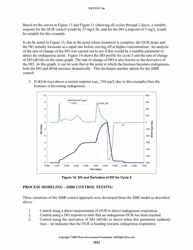
Based on the curves in Figure 13 and Figure 11 (showing all cycles through 2 days), a suitable setpoint for the OUR control would be 35 mg/L/hr, and for the DO a setpoint of 5 mg/L would be suitable for this example. It can be noted in Figure 13, that at the point where treatment is complete, the OUR drops and the DO initially increases at a rapid rate before curving off at higher concentrations. An analysis of the rate of change of the DO was carried out to see if this would be a suitable parameter to detect the endogenous point. Figure 14 shows the DO profile for cycle 5 and the rate of change of DO (dO/dt) on the same graph. The rate of change of DO is also known as the derivative of the DO. In this graph, it can be seen that at the point at which the biomass becomes endogenous, both the DO and dO/dt increase dramatically. This facilitates another option for the iSBR control:

3. If dO/dt rises above a certain setpoint (say, 250 mg/L/day in this example) then the biomass is becoming endogenous.

0.903, 281

0

1

2

3

4

5

6

7

8

9

10

0.800 0.820 0.840 0.860 0.880 0.900 0.920 0.940 0.960 0.980 1.000

Time (days)

DO

(mg/

L)

-600

-500

-400

-300

-200

-100

0

100

200

300

400

dO/d

t (m

g/L/

day)

Dissolved OxygendO/dt

Figure 14: DO and Derivative of DO for Cycle 5

PROCESS MODELING – iSBR CONTROL TESTING Three variations of the iSBR control approach were developed from the SBR model as described above:

1. Control using a direct measurement of OUR to detect endogenous respiration. 2. Control using a DO setpoint to infer that an endogenous OUR has been reached. 3. Control using the derivative of DO (dO/dt) to detect when this parameter suddenly

rises – an indicator that the OUR is heading towards endogenous respiration.

7031

WEFTEC®.06


The GPS-X model used to assess the plant capacity was modified to test the effectiveness of the three different control approaches to detect the endogenous point. Figure 6 shows a red toolbox icon in the model layout. This toolbox contains an on/off controller that uses one of the 3 parameters listed above to switch off the blower once a setpoint has been reached. In addition to adding this toolbox icon, some user code was added to the model to carry out the endogenous detection only when the model was in the aerate phase (phase number 4 in the model). The model was operated using each control parameter for a period of three days and the outputs compared. All three control approaches detected the endogenous point correctly and proved suitable for further investigation. DO and OUR profiles from the three control approaches are shown in Figures 15 through 17. (Compare with Figure 11 which is the case with no control).

0

1

2

3

4

5

6

7

8

9

10

0.0 0.5 1.0 1.5 2.0

Time (days)

DO

(mg/

L)

0

10

20

30

40

50

60

70

80

90

100

OU

R (m

g/L/

hr)

Dissolved Oxygen OUR (Actual)

Figure 15: OUR Control - DO and OUR profile

7032

WEFTEC®.06


0

1

2

3

4

5

6

7

8

9

10

0.0 0.5 1.0 1.5 2.0

Time (days)

DO

(mg/

L)

0

10

20

30

40

50

60

70

80

90

100

OU

R (m

g/L/

hr)


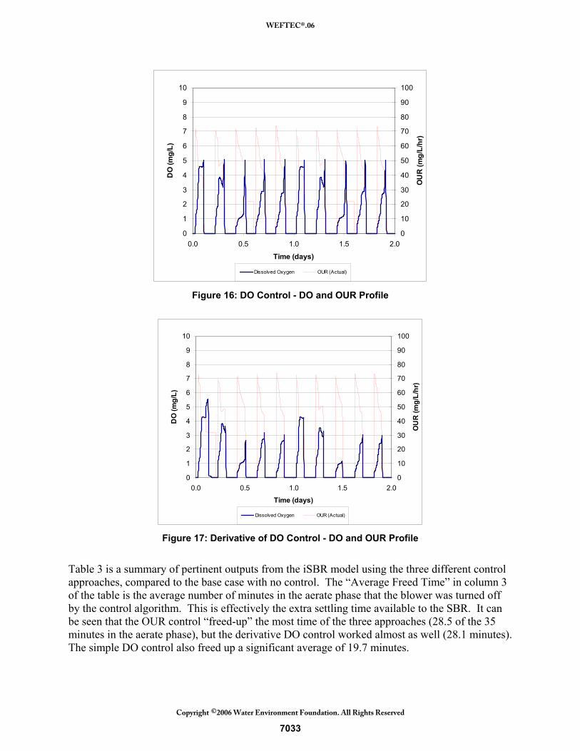
Figure 16: DO Control - DO and OUR Profile

0

1

2

3

4

5

6

7

8

9

10

0.0 0.5 1.0 1.5 2.0

Time (days)

DO

(mg/

L)

0

10

20

30

40

50

60

70

80

90

100

OU

R (m

g/L/

hr)


Figure 17: Derivative of DO Control - DO and OUR Profile

Table 3 is a summary of pertinent outputs from the iSBR model using the three different control approaches, compared to the base case with no control. The “Average Freed Time” in column 3 of the table is the average number of minutes in the aerate phase that the blower was turned off by the control algorithm. This is effectively the extra settling time available to the SBR. It can be seen that the OUR control “freed-up” the most time of the three approaches (28.5 of the 35 minutes in the aerate phase), but the derivative DO control worked almost as well (28.1 minutes). The simple DO control also freed up a significant average of 19.7 minutes.

7033

WEFTEC®.06


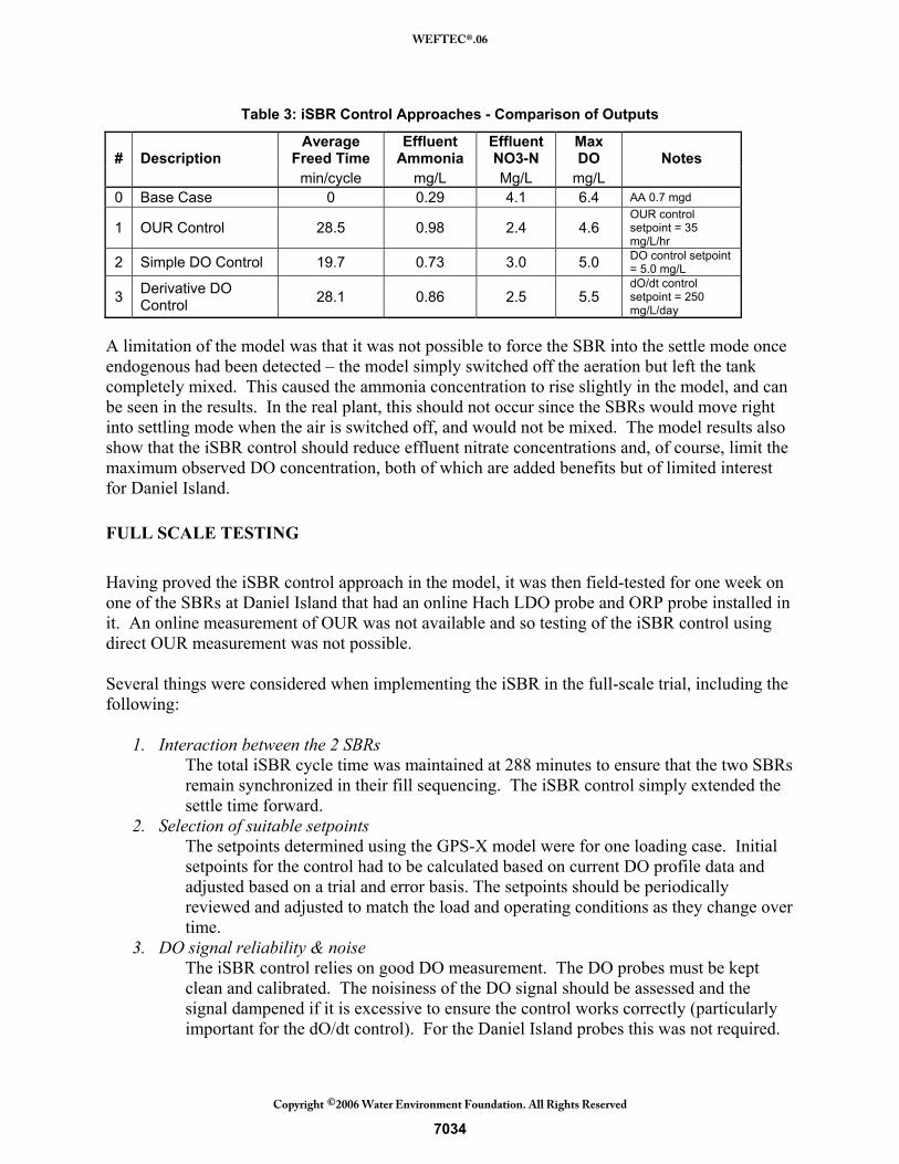
Table 3: iSBR Control Approaches - Comparison of Outputs

# Description Average

Freed Time Effluent

Ammonia Effluent NO3-N

Max DO Notes

min/cycle mg/L Mg/L mg/L 0 Base Case 0 0.29 4.1 6.4 AA 0.7 mgd

1 OUR Control 28.5 0.98 2.4 4.6 OUR control setpoint = 35 mg/L/hr

2 Simple DO Control 19.7 0.73 3.0 5.0 DO control setpoint = 5.0 mg/L

3 Derivative DO Control 28.1 0.86 2.5 5.5

dO/dt control setpoint = 250 mg/L/day

A limitation of the model was that it was not possible to force the SBR into the settle mode once endogenous had been detected – the model simply switched off the aeration but left the tank completely mixed. This caused the ammonia concentration to rise slightly in the model, and can be seen in the results. In the real plant, this should not occur since the SBRs would move right into settling mode when the air is switched off, and would not be mixed. The model results also show that the iSBR control should reduce effluent nitrate concentrations and, of course, limit the maximum observed DO concentration, both of which are added benefits but of limited interest for Daniel Island. FULL SCALE TESTING Having proved the iSBR control approach in the model, it was then field-tested for one week on one of the SBRs at Daniel Island that had an online Hach LDO probe and ORP probe installed in it. An online measurement of OUR was not available and so testing of the iSBR control using direct OUR measurement was not possible. Several things were considered when implementing the iSBR in the full-scale trial, including the following:

1. Interaction between the 2 SBRs The total iSBR cycle time was maintained at 288 minutes to ensure that the two SBRs remain synchronized in their fill sequencing. The iSBR control simply extended the settle time forward.

2. Selection of suitable setpoints The setpoints determined using the GPS-X model were for one loading case. Initial setpoints for the control had to be calculated based on current DO profile data and adjusted based on a trial and error basis. The setpoints should be periodically reviewed and adjusted to match the load and operating conditions as they change over time.

3. DO signal reliability & noise The iSBR control relies on good DO measurement. The DO probes must be kept clean and calibrated. The noisiness of the DO signal should be assessed and the signal dampened if it is excessive to ensure the control works correctly (particularly important for the dO/dt control). For the Daniel Island probes this was not required.

7034

WEFTEC®.06


4. Sludge Settling The settling characteristics of the sludge are critical to the performance of the plant and directly impact the required settling time. The SVI and MLSS of the sludge were carefully monitored throughout the trial.

5. Storm Mode Implementation of the iSBR algorithm in the PLC controller had to ensure that the storm mode operation was still fully functional. The iSBR control algorithm is designed for normal dry weather treatment and not peak day flows.

Test Protocol The purpose of the site trial was to prove the iSBR control concept. It did not directly assess the plant capacity but information gathered from the trial was used to verify the process enhancements predicted by the modeling. One SBR was operated using the iSBR control (SBR#1): the other continued with its normal operation without iSBR control (SBR#2). The simple DO and derivate DO iSBR control approaches were tested over a period of 4 days. The iSBR control was used to extend the settling time by shutting off the blowers when an endogenous point was reached; overall cycle times will remain the same. DO and ORP were monitored continuously for each SBR and recorded in the plant SCADA system.

Originally it had been intended to test the two control approaches for two days each however the schedule had to be modified slightly because the plant had a blower belt failure on the weekend prior to the testing and it took the plant a couple of days to fully recover. It was decided that the simple DO control test should be extended until Thursday, August 17th to provide more opportunities for endogenous detection and the dO/dt control was tested for just one day from Thursday to Friday. Sampling of the decant water and sludge blanket measurements were carried out on Monday, Wednesday and Thursday, with the most intensive analysis occurring on the Wednesday. Monitoring of DO, ORP and tank level was continuous throughout the week using the plant SCADA system. iSBR control was tested on SBR #1 and SBR #2 continued with it’s normal operation. Simple DO Control. The control algorithm for the simple DO control was added to the SBR PLC program by CPW staff. In this control approach, the control logic monitors the DO concentration during the react phase (aerate without fill) and if the DO increases above a user-defined set point, the code shuts down the blowers until the end of the react cycle. The remainder of the react cycle then becomes an extension to the start of the settle phase. The code also includes a user defined delay to prevent the code from being initiated too soon in the react cycle. For the test period, the delay was set to 300 seconds (5 minutes). Figure 18 shows the historical DO profile for SBR #1 for approximately 3 weeks prior to the iSBR testing. It can be seen that the DO readings stayed at or below 1 mg/L for most of the period except for a multitude of spikes up to much higher DO concentrations. These spikes are indications that the activated sludge has become endogenous during the react phase. From this data, a set point of 2.5 mg/L was chosen as the trigger point for the simple DO control to detect endogenous. Note also that the DO never dropped below 0.5 mg/L even during unaerated phases, indicating that the DO offset was not set correctly.

7035

WEFTEC®.06


Simple DO control was turned on at 10 am on Monday, August 15th although it did not initiate a control action until Tuesday afternoon because the SBR did not reach endogenous conditions in any of its cycles until then because the plant was recovering from the blower belt failure over the weekend.

Daniel Island SBR#1 Historical DO

0.0

1.0

2.0

3.0

4.0

5.0

6.0

7.0

07/27/05 08/03/05 08/10/05

Date

DO

(mg/

L)

Figure 18: Historical DO Profile Prior to iSBR Testing

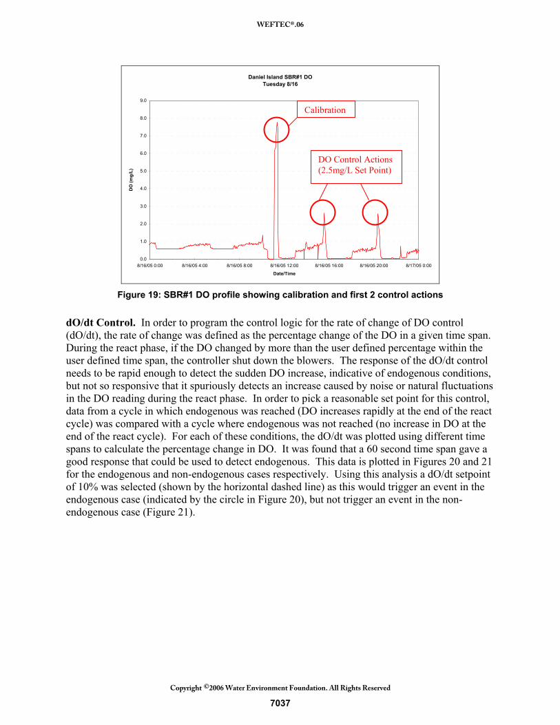
At approximately 11:30 am Tuesday morning, the DO probe in SBR #1 was removed, cleaned and calibrated. The zero offset was also reset back to 0 mg/L. This can be seen in Figure 19 which is a plot of the DO for Tuesday. There is a definite spike up to 7.8 mg/L, which is the oxygen saturation concentration at the probe’s temperature of 31.8ºC at that time, and the DO drops down to 0 mg/L when the probe was returned to the basin prior to aeration. On the same figure, the first two control actions can be seen, with the DO rising to 2.5 mg/L before the control program shut down the blowers, causing the DO to drop. In order to assist the SBR to reach endogenous in the first of these actions, the react phase was extended by 35 minutes by resetting the PLC control (which causes the control to restart filling SBR #2 whilst restarting the react phase for SBR #1).

7036

WEFTEC®.06


Daniel Island SBR#1 DOTuesday 8/16

0.0

1.0

2.0

3.0

4.0

5.0

6.0

7.0

8.0

9.0

8/16/05 0:00 8/16/05 4:00 8/16/05 8:00 8/16/05 12:00 8/16/05 16:00 8/16/05 20:00 8/17/05 0:00

Date/Time

DO

(mg/

L)

Figure 19: SBR#1 DO profile showing calibration and first 2 control actions

dO/dt Control. In order to program the control logic for the rate of change of DO control (dO/dt), the rate of change was defined as the percentage change of the DO in a given time span. During the react phase, if the DO changed by more than the user defined percentage within the user defined time span, the controller shut down the blowers. The response of the dO/dt control needs to be rapid enough to detect the sudden DO increase, indicative of endogenous conditions, but not so responsive that it spuriously detects an increase caused by noise or natural fluctuations in the DO reading during the react phase. In order to pick a reasonable set point for this control, data from a cycle in which endogenous was reached (DO increases rapidly at the end of the react cycle) was compared with a cycle where endogenous was not reached (no increase in DO at the end of the react cycle). For each of these conditions, the dO/dt was plotted using different time spans to calculate the percentage change in DO. It was found that a 60 second time span gave a good response that could be used to detect endogenous. This data is plotted in Figures 20 and 21 for the endogenous and non-endogenous cases respectively. Using this analysis a dO/dt setpoint of 10% was selected (shown by the horizontal dashed line) as this would trigger an event in the endogenous case (indicated by the circle in Figure 20), but not trigger an event in the non-endogenous case (Figure 21).

Calibration

DO Control Actions (2.5mg/L Set Point)

7037

WEFTEC®.06


DO and dO/dtCase 1 - Endogenous Reached (DO spike)

10

0.0

0.5

1.0

1.5

2.0

2.5

3.0

3.5

4.0

8/17/05 16:48 8/17/05 18:00 8/17/05 19:12 8/17/05 20:24 8/17/05 21:36 8/17/05 22:48

Date/Time

DO

(mg/

L)

-30

-20

-10

0

10

20

30

DO

Cha

nge

(%)

DO

Control Line

dO/dt (% Change)

Figure 20: dO/dt and DO for an endogenous event

DO and dO/dt

Case 2 - Endogenous Not Reached (No DO spike)

10 10

0.0

0.5

1.0

1.5

2.0

2.5

3.0

3.5

4.0

8/17/05 8:24 8/17/05 8:52 8/17/05 9:21 8/17/05 9:50 8/17/05 10:19 8/17/05 10:48 8/17/05 11:16 8/17/05 11:45

Date/Time

DO

(mg/

L)

-30

-20

-10

0

10

20

30

DO

Cha

nge

(%)

DO

Control Line

dO/dt (% Change)

Figure 21: dO/dt and DO with no endogenous event

dO/dt control was tested from Thursday, August 17th at 13:05 until Friday at 9:00 am. Following this test work SBR#1 was put back into simple DO control mode to check for longer term effects on the activated sludge settling characteristics. Field Test Results and Observations Figure 22 shows the tank level (at top in green) and DO (red at bottom) on the left Y-axis and ORP (blue in center) on the right Y-axis for the whole test week. It can be seen that there are several spikes in the DO readings, though they are much lower than the spikes seen in historical data (Figure 18) due to the action of the iSBR control algorithms. The DO is generally at or below the setpoint of 2.5 mg/L except for exceptionally low loaded periods overnight when the

7038

WEFTEC®.06


DO rises while still filling prior to the react phase and the large spike on Tuesday morning caused by the probe calibration. From this figure it can also be seen that, as expected, the ORP follows a similar pattern to the DO profile.

Daniel Island SBR#1Test Week 8/15 - 8/19

0.0

2.0

4.0

6.0

8.0

10.0

12.0

14.0

16.0

18.0

8/15/050:00

8/15/0512:00

8/16/050:00

8/16/0512:00

8/17/050:00

8/17/0512:00

8/18/050:00

8/18/0512:00

8/19/050:00

8/19/0512:00

Date/Time

Hei

ght &

DO

(ft &

mg/

L)

-300

-250

-200

-150

-100

-50

0

50

100

150

200

OR

P (m

V) LevelDOORP

Figure 22: SBR #1 SCADA data for Test Week

The focal day for assessing the simple DO iSBR control was Wednesday, August 18th. Figure 23 shows the DO and ORP profile for this day. It can be seen that 3 of the 5 cycles have DO peaks that caused the DO control to cut off the blowers at about 2.5 mg/L, showing that the control worked successfully. The second cycle of the day (where aeration starts just before 4 am) shows an elevated DO through the end of the react/fill phase as the load is so low during this time, the SBR becomes endogenous even through it is still being filled. The jagged shape of the DO profile in this particular cycle is attributed to the influent pumps kicking on intermittently through the early hours of the day. During this cycle the simple DO control was able to shut off the blowers soon after the SBR went into the react phase (after the user defined 5 minute delay). This figure shows more clearly, the ORP profile next to the DO. It could be possible to control the react cycle using ORP as an alternative to DO, however the curve is slightly more complex because ORP is influenced by oxidative and reductive species other than DO. In this study, ORP control was not considered and the readings are provided for information only.

7039

WEFTEC®.06


Daniel Island SBR#1Wednesday 8/17

0.0

1.0

2.0

3.0

4.0

5.0

6.0

7.0

8.0

9.0

8/17/05 0:00 8/17/05 4:00 8/17/05 8:00 8/17/05 12:00 8/17/05 16:00 8/17/05 20:00 8/18/05 0:00

Date/Time

DO

(mg/

L)

-300

-250

-200

-150

-100

-50

0

50

100

150

200

OR

P (m

V)

DOORP

Figure 23: SBR#1 DO and ORP for Wednesday 8/17/2005

The fourth cycle of the day (starting at approximately 12:30 pm) is shown in more detail in Figure 24. During the react phase for this cycle, additional measurements were taken, namely, ammonia was measured from filtered grab samples every 10 minutes using the plant’s Hach colorimetric test kit and the DO was measured manually using the plant’s handheld YSI probe. At the end of the react phase for this cycle it was evident that ammonia concentrations were dropping close to 1 mg/L. It appeared that a further 35 minutes of aeration would probably enable the SBR to reach endogenous and so the react phase was extended by 35 minutes (labeled “Extended Aerate”).

Daniel Island SBR #1Detailed iSBR Analysis 8/17/05

Fill Fill/Aerate Aerate

Exte

nded

Aer

ate

Settle Decant

0.0

0.5

1.0

1.5

2.0

2.5

3.0

3.5

4.0

4.5

5.0

12:00 13:00 14:00 15:00 16:00 17:00 18:00 19:00

Time

DO

& A

mm

onia

(mg/

L)

-100

-50

0

50

100

150

200

OR

P (m

V)

Online DO mg/LiSBR TriggerAmmonia ProfileYSI DOORP mV

Figure 24: Detail of cycle 4 on Wednesday including ammonia profile and YSI DO

7040

WEFTEC®.06


In Figure 24 it can be seen that the rapid increase in DO occurs when the ammonia concentration reaches zero. This is because nitrification exerts a significant proportion of the oxygen demand observed in the SBR and at the point where all the ammonia is used up, the oxygen demand falls rapidly and so the DO increases. This figure also shows that the ORP curve doesn’t respond quite as rapidly as the DO curve. Finally, from this figure it can be seen that the online DO measurement using the Hach LDO is similar to the readings from the handheld YSI probe, with the YSI reading slightly higher than the Hach LDO. During each decant phase for both SBR #1 (with iSBR control) and SBR#2, samples were taken from the clear liquid layer at the start and the end of their decant cycles and analyzed for ammonia, nitrate and nitrite, to see if they changed significantly. In addition, the samples were also measured for BOD and TSS in order to estimate the change in soluble BOD. Figure 25 shows an example of the transformations in nitrogen concentrations from the start of the decant to the end. In all of the samples that were gathered – including the example in Figure 25 – there is a notable decrease in the nitrate concentration and a slight increase in the ammonia from the start to the end of the decant phase.

Nitrogen Concentrations Through DecantSBR#1, 8/17/2005 17:25 (iSBR Initiated)

36

29

0.380.21

0.55

0.44

0

5

10

15

20

25

30

35

40

Decant Start Decant End

mg/

L

Nitrite

Nitrate

Ammonia

Figure 25: Example of nitrogen transformations during decant

Table 4 is a summary of the nitrogen nutrient changes for all the decant phases for which samples were taken, comparing the results from SBR#1 and SBR #2. The results for SBR#1 for the cases where the iSBR control was initiated (i.e. the control stopped the blowers) are also shown separately in the center column. The top section of the table shows the average initial nutrient concentrations at the start of the decant cycle and the lower section shows the overall change in nutrient and soluble BOD concentrations expressed as the rate in mg/L/hr.

7041

WEFTEC®.06


Table 4: Nutrient Changes During Decant

SBR #1 (all data)1

SBR #1 (iSBR

initiated) SBR #21

Initial Concentrations (mgN/L) Average Ammonia 1.4 0.2 0.4 Average Nitrate 24.7 22.3 30.3 Average Nitrite 0.5 0.4 0.2

Change During Decant2 (mgN/L/hr) Ammonia 0.34 0.22 0.27 Nitrate+Nitrite -6.3 -7.5 -12.9 soluble BOD3 -1.2 -0.8 0.4

Notes: 1 Total of 4 samples taken for SBR#1, of which 2 occurred after iSBR initiated and 3 samples for SBR #2. Data for 8/15 not included.

2 +ve value = increase during decant, -ve = decrease during decant 3 Estimated from BOD and TSS data

From this data, some general observations can be made:

1. The iSBR appears to have a lower nitrate concentration, which is due to the fact that it has longer unaerated (anoxic) phases than the non-iSBR unit.

2. A significant reduction in the nitrate concentration is observed in both SBRs during the decant.

3. Changes in other nutrients, including ammonia, and soluble BOD are insignificant. The iSBR control does not cause any additional ammonia or soluble BOD to be released. In addition to taking samples at the start and end of the decant cycles, the sludge blanket and liquid levels were measured. From this data, the average blanket settling rates were calculated for the settle and decant phases. This information is summarized in Table 5.

Table 5: Blanket and Liquid Level Changes

SBR #1 SBR #1 SBR #2

(all data) (iSBR

initiated) Average Blanket Level (ft)

At Start of Decant 12.2 11.1 12.7 After Decant 9.6 9.3 10.2

Average Blanket Settling Rate (ft/hr) During Settle 3.5 3.8 3.4 During Decant 3.7 3.1 3.6

Decant Rate Liquid descent (ft/hr) 5.1 4.3 5.1 Equivalent flow (gpm) 1240 1052 1256

It appears that, on average, the blanket in SBR 1 was slightly lower than for SBR 2 by about 0.5 ft, which is likely due to the extended settling period at the end of the react phase. The actual blanket settling rates were similar between SBRs 1 and 2. Also listed in the table for information purposes, is the decant rate expressed as the rate at which the liquid level descended (labeled

7042

WEFTEC®.06


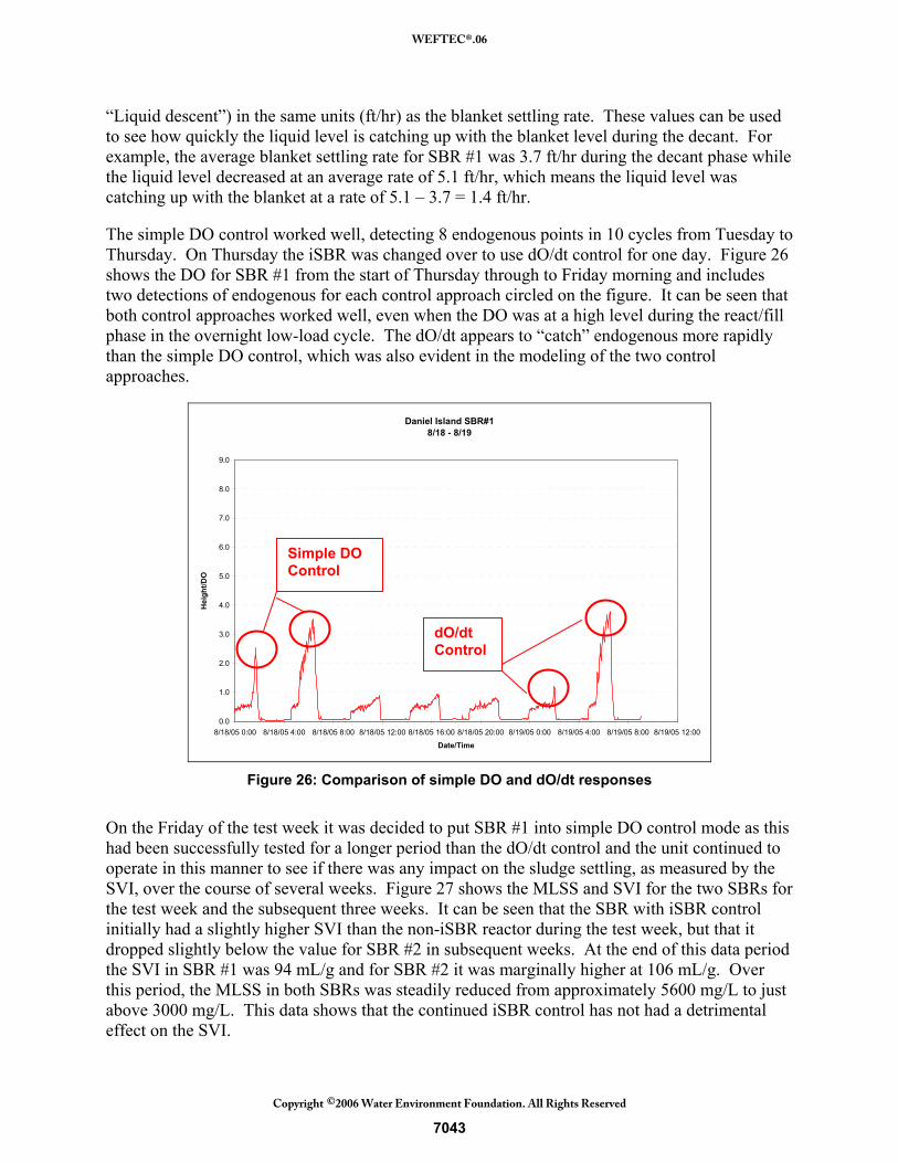
“Liquid descent”) in the same units (ft/hr) as the blanket settling rate. These values can be used to see how quickly the liquid level is catching up with the blanket level during the decant. For example, the average blanket settling rate for SBR #1 was 3.7 ft/hr during the decant phase while the liquid level decreased at an average rate of 5.1 ft/hr, which means the liquid level was catching up with the blanket at a rate of 5.1 – 3.7 = 1.4 ft/hr. The simple DO control worked well, detecting 8 endogenous points in 10 cycles from Tuesday to Thursday. On Thursday the iSBR was changed over to use dO/dt control for one day. Figure 26 shows the DO for SBR #1 from the start of Thursday through to Friday morning and includes two detections of endogenous for each control approach circled on the figure. It can be seen that both control approaches worked well, even when the DO was at a high level during the react/fill phase in the overnight low-load cycle. The dO/dt appears to “catch” endogenous more rapidly than the simple DO control, which was also evident in the modeling of the two control approaches.

Daniel Island SBR#18/18 - 8/19

0.0

1.0

2.0

3.0

4.0

5.0

6.0

7.0

8.0

9.0

8/18/05 0:00 8/18/05 4:00 8/18/05 8:00 8/18/05 12:00 8/18/05 16:00 8/18/05 20:00 8/19/05 0:00 8/19/05 4:00 8/19/05 8:00 8/19/05 12:00

Date/Time

Hei

ght/D

O

Figure 26: Comparison of simple DO and dO/dt responses

On the Friday of the test week it was decided to put SBR #1 into simple DO control mode as this had been successfully tested for a longer period than the dO/dt control and the unit continued to operate in this manner to see if there was any impact on the sludge settling, as measured by the SVI, over the course of several weeks. Figure 27 shows the MLSS and SVI for the two SBRs for the test week and the subsequent three weeks. It can be seen that the SBR with iSBR control initially had a slightly higher SVI than the non-iSBR reactor during the test week, but that it dropped slightly below the value for SBR #2 in subsequent weeks. At the end of this data period the SVI in SBR #1 was 94 mL/g and for SBR #2 it was marginally higher at 106 mL/g. Over this period, the MLSS in both SBRs was steadily reduced from approximately 5600 mg/L to just above 3000 mg/L. This data shows that the continued iSBR control has not had a detrimental effect on the SVI.

Simple DO Control

dO/dt Control

7043

WEFTEC®.06


Daniel Island SBRsMLSS and SVI Subsequent to iSBR Control Start

Test Week

SBR #1 SVI, 94

SBR #2 SVI, 106

0

1000

2000

3000

4000

5000

6000

7000

8000

9000

10000

14-Aug 21-Aug 28-Aug 4-Sep 11-Sep

Date

MLS

S (m

g/L)

0

20

40

60

80

100

120

140

SVI (

mL/

g)

SBR#1 MLSSSBR#2 MLSSSBR #1 SVISBR #2 SVI

Figure 27: Long term SVI and MLSS data for continued iSBR operation

(SBR #1 has iSBR control in simple DO mode)

CONCLUSION The full-scale trial proved very successful using either the DO or the dO/dt approach. iSBR control was continued beyond the initial one week trial and the second SBR has since been converted to do the same. The study enabled the plant to be rerated to 0.75 mgd with the addition of extra aeration capacity and further to 1.0 mgd using an influent equalization tank. The South Carolina Department of Health and Environmental Control has issued revised NPDES Permits to reflect the increased capacity of the facility, once the additional equipment has been added to the plant. A construction project is currently underway to modify the facility. REFERENCES Andreottola, G., Foladori, P. and Ragazzi, M. (2001) "On-line control of a SBR system for nitrogen removal from industrial wastewater" Wat. Sci. Tech Vol 43 No 3 pp 93-100 Barnard J.L., Shaw, A. and Watts, J.B. (2003) "Optimized Control of Nitrifying Suspended Growth Systems Using Respirometry," Proceedings of Ozwater 2003 Convention & Exhibition, AWA 20th Convention, Perth, Australia. Cho, B.C., Chang, C.N., Liaw, S.L. and Huang, P.T. (2001) "The feasible sequential control strategy of treating high strength organic nitrogen wastewater with sequencing batch biofilm reactor," Wat. Sci. Tech. Vol 43 No 3 pp 115-122

7044

WEFTEC®.06


Cohen, A., Hegg, D., de Michele, M., Song, Q. and Kasabov, N. (2003) "An intelligent controller for automated operation of sequencing batch reactors," Wat. Sci. Tech. Vol. 47, No.12, pp57-63 Demoulin, G., Goronszy, M.C., Wutscher, K. and Forsthuber, E. (1997). "Co-Current Nitrification/Denitrification and Biological P-Removal in Cyclic Activated Sludge Plants by Redox Controlled Cycle Operation" Wat.Sci. Tech., 35(1), 215. GPS-X Technical Reference Manual. Version 4.1 (2003), Hyromantis Inc., Ontario, Canada Shaw, A., Mason, L. and Miller, R. (2001) “The Use of Online Respirometric Monitoring and Dose Response Testing to Determine the Best Process Alternatives for an Existing Petrochemical Waste Treatment Facility”, Water Environment Federation 74th Annual Conference, Atlanta, Georgia, October 2001 Shaw, A. and Watts, J.B. (2002) “The Use of Respirometry for the Control of Sequencing Batch Reactors: Principles and Practical Application”, Water Environment Federation 75th Annual Conference, Chicago, Illinois, September 2002. Shaw, A. (2003) “Using On-Line Oxygen Uptake Rates for Monitoring and Control of Activated Sludge Processes”, Water Environment Federation 76th Annual Conference. Pre-conference workshop: Using Respirometers for Design and Operation of Biological Wastewater Treatment Plants, Los Angeles, California. October 2003 Yoong, E.T., Lant, P.A. and Greenfield, P.F. (2000) "In Situ Respirometry in an SBR Treating Wastewater with High Phenol Concentrations," Wat. Res. Vol. 34 No.1, pp 239-245

7045

WEFTEC®.06


development and field testing of a new intelligent

Documents