development and evaluation of fully automated demand
TRANSCRIPT

CALIFORNIAENERGYCOMMISSION
DEVELOPMENT AND EVALUATION OFFULLY AUTOMATED DEMAND RESPONSE
IN LARGE FACILITIES
PIE
R C
OL
LA
BO
RA
TIV
E R
EP
OR
T
January 2005CEC-500-2005-013

Prepared By: Mary Ann PietteLawrence Berkeley National LaboratoryBerkeley, California
Contract No. 150-99-003
Prepared For:
California Energy CommissionPublic Interest Energy Research (PIER) Program
Laurie tenHopeContract Manager
Laurie tenHopeProgram Area Team Lead
Ron Kukulka,Acting Deputy DirectorENERGY RESEARCH AND DEVELOPMENTDIVISION
Robert L. TherkelsenExecutive Director
The work described in this report was coordinated bythe Consortium for Electric Reliability TechnologySolutions and funded by the California EnergyCommission, Public Interest Energy ResearchProgram, under Work for Others Contract No. 150-99-003, Am #1 and by the U.S. Department of Energyunder Contract No. DE-AC03-76SF00098.
DISCLAIMERThis report was prepared as the result of work sponsored by theCalifornia Energy Commission. It does not necessarily representthe views of the Energy Commission, its employees or the Stateof California. The Energy Commission, the State of California, itsemployees, contractors and subcontractors make no warrant,express or implied, and assume no legal liability for theinformation in this report; nor does any party represent that theuses of this information will not infringe upon privately ownedrights. This report has not been approved or disapproved by theCalifornia Energy Commission nor has the California EnergyCommission passed upon the accuracy or adequacy of theinformation in this report.

PREFACE
The Public Interest Energy Research (PIER) Program supports public interest energyresearch and development that will help improve the quality of life in California bybringing environmentally safe, affordable, and reliable energy services and products tothe marketplace.
The PIER Program, managed by the California Energy Commission (Commission),annually awards up to $62 million to conduct the most promising public interest energyresearch by partnering with Research, Development, and Demonstration (RD&D)organizations, including individuals, businesses, utilities, and public or private researchinstitutions.
• PIER funding efforts are focused on the following six RD&D program areas:
• Buildings End-Use Energy Efficiency
• Industrial/Agricultural/Water End-Use Energy Efficiency
• Renewable Energy
• Environmentally-Preferred Advanced Generation
• Energy-Related Environmental Research
• Strategic Energy Research.
What follows is the final report for the Building Vulnerability Guide, 500-01-034,conducted by the Lawrence Berkeley National Laboratory. The report is entitledBuilding Vulnerability Assessment and Mitigation. This project contributes to theBuildings Program.
For more information on the PIER Program, please visit the Commission's Web site at:http://www.energy.ca.gov/research/index.html or contact the Commission'sPublications Unit at 916-654-5200.

Full LBNL Disclaimer
DISCLAIMER
This document was prepared as an account of work sponsored by the United StatesGovernment. While this document is believed to contain correct information, neither theUnited States Government nor any agency thereof, nor The Regents of the University ofCalifornia, nor any of their employees, makes any warranty, express or implied, orassumes any legal responsibility for the accuracy, completeness, or usefulness of anyinformation, apparatus, product, or process disclosed, or represents that its use would notinfringe privately owned rights. Reference herein to any specific commercial product,process, or service by its trade name, trademark, manufacturer, or otherwise, does notnecessarily constitute or imply its endorsement, recommendation, or favoring by theUnited States Government or any agency thereof, or The Regents of the University ofCalifornia. The views and opinions of authors expressed herein do not necessarily state orreflect those of the United States Government or any agency thereof, or The Regents ofthe University of California.
Ernest Orlando Lawrence Berkeley National Laboratory is an equal opportunityemployer.
Abbreviated LBNL Disclaimer (place under CEC disclaimer)
This work was also supported by the Assistant Secretary for Energy Efficiencyand Renewable Energy, Building Technologies Program, of the US Departmentof Energy under Contract No. DE-AC03-76SF00098.

Development and Evaluation of Fully AutomatedDemand Response In Large Facilities
March 30, 2004
Mary Ann PietteOsman Sezgen
David S. WatsonNaoya Motegi
Lawrence Berkeley National Laboratory
Christine ShockmanShockman Consulting
Laurie ten HopeProgram Manager, Energy Systems Integration
Sponsored by the California Energy Commission


Table of Contents
Table of Contents ........................................................................................................... iList of Tables and Figures ............................................................................................ iiAcknowledgements ....................................................................................................... vEXECUTIVE SUMMARY....................................................................................... E-1
1. Introduction....................................................................................................... 11-1 Background and Report Overview ............................................................... 11-2 Project Goals ............................................................................................... 21-3 Previous Research........................................................................................ 3
2. Methodology ...................................................................................................... 72-1 Project Overview and Timeline.................................................................... 72-2 Selection Criteria and Sites Considered........................................................ 82-3 Site Characteristics and Background ............................................................ 92-4 Automated Demand Response System Description .................................... 152-5 Controls and Communications Upgrades ................................................... 182-6 Electric Price Signal and Test Description ................................................. 192-7 Assessment of Lead Users of Auto-DR...................................................... 20
3. Auto-DR Systems Characterization and Measurement................................. 233-1 Auto-DR System Architecture ................................................................... 233-2 Site Measurement and Evaluation Techniques ........................................... 44
4. Results.............................................................................................................. 504-1 Requesting and Confirming Receipt of Signal............................................ 504-2 Demand Shed Savings Estimates ............................................................... 50
5. Discussion: Organizational and Technological Issues.................................... 725-1 Implementation and Organizational Challenges ......................................... 725-2 Overview of Technical Challenges............................................................. 735-3 Lessons from each Site .............................................................................. 745-4 State of the Art Auto-DR Systems ............................................................. 77
6. Summary and Future Research Topics .......................................................... 80
7. References........................................................................................................ 84
APPENDICESAppendix I. Acronyms and Terminology.....................................................I-1
Appendix II. Methodology – Additional Details ......................................... II-1Appendix II-1. Whole-Building Level Method, Additional Detail .................... II-1
Appendix III. Sample Memorandum of Understanding .............................III-1Appendix III-1. Project Participant Memorandum of Understanding................. III-1Appendix III-2. Automated Demand Response Test Questionnaire................... III-4Appendix III-3. Time Schedule for Demand Response Test Participants........... III-6Appendix III-4. Price Signal for the Automated Demand Responses Tests........ III-7

Appendix III-5. RT Pricing Web Methods and XML Schema......................... III-10
Appendix IV. Participants List ....................................................................IV-1
Appendix V. Site Questionnaires (Test 1, Test 2) ....................................... V-1Appendix V-1. Site Questionnaires – Albertsons .............................................. V-1Appendix V-2. Site Questionnaires – Bank of America .................................... V-3Appendix V-3. Site Questionnaires – GSA Oakland ......................................... V-5Appendix V-4. Site Questionnaires – Roche ..................................................... V-8Appendix V-5. Site Questionnaires – UCSB................................................... V-10
Appendix VI. Site Data Collection Points List ............................................VI-1Appendix VI-1. Albertsons – Point List ............................................................ VI-1Appendix VI-2. Bank of America – Point List .................................................. VI-1Appendix VI-3. GSA Oakland – Point List ....................................................... VI-3Appendix VI-4. Roche – Point List and Fan Spot Measurement Plan ................ VI-5Appendix VI-5. UCSB – Shed Strategies and Point List ................................... VI-9
Appendix VII. Additional Result Tables and Figures ................................ VII-1Appendix VII-1. First Day Test Results ............................................................VII-1Appendix VII-2. B of A – Result Analysis by WebGen.....................................VII-5Appendix VII-3. GSA – Additional Figures ......................................................VII-7Appendix VII-4. Roche – Additional Figures ..................................................VII-17Appendix VII-5. UCSB – Additional Figures..................................................VII-19
Appendix VIII. Previous DR Participation and Site Contact .....................VIII-1Appendix VIII-1. Prior Demand Response Program Participation .................... VIII-1Appendix VIII-2. Interaction with Site Contacts............................................... VIII-4Appendix VIII-3. Problems Encountered During Test Period ........................... VIII-8
List of Tables and Figures
Table 2-1. Project Timeline and Milestones .............................................................. 7Table 2-2. Summary of Sites................................................................................... 10Table 3-1. Characteristics of Auto-DR Systems - Architecture................................ 24Table 3-2. Characteristics of Auto-DR Systems - Gateways.................................... 25Table 3-3. Characteristics of Auto-DR Systems - Integration .................................. 28Table 3-4. Characteristics of Auto-DR Systems - Shed Control............................... 29Table 3-5. Characteristics of Auto-DR Systems - Open Standards .......................... 30Table 3-6. Oakland GSA Zone Temperature Setpoints - Normal and Shed Modes .. 37Table 3-7. Measurement Summary ......................................................................... 44Table 3-8. Component Level Methods for Each Component ................................... 48Table 4-1. Record of Prices Being Requested and Receipt Being Confirmed .......... 50Table 4-2. Shed Strategies and Results of Response................................................ 51Table 4-3. UCSB –Estimated Savings by Component (Component Method)........... 65Table 4-4. Summary of Estimated Savings of All Site (Whole-Building Method) ... 68

Table 4-5. Summary of Estimated Savings of All Site (Component Method) .......... 68
Figure E-1. Fictitious Electric Price Signal Sent to Five Facilities............................... 2Figure E-2. Geographical Location of Auto-DR Infrastructure.................................... 3Figure E-3. Auto-DR Electric Load Shed from five sites on Wed. Nov. 19, 2003. ...... 3Figure E-4. Auto-DR Electric Load Shed from five sites on Wed. Nov. 19, 2003. ...... 4
Figure 1-1. Overlap Between Energy Information Systems (EIS), Energy ManagementControl Systems (EMCS) and Demand Response Systems (DRS)............ 5
Figure 2-1. Albertsons.............................................................................................. 11Figure 2-2. Bank of America - Concord Data Center, Building B............................. 12Figure 2-3. GSA Oakland Federal Building.............................................................. 12Figure 2-4. Roche Palo Alto – Building FS (left) and A2 (right)............................... 13Figure 2-5. UCSB – Davidson Library ..................................................................... 14Figure 2-6. Auto-DR Network Communications Sequence....................................... 15Figure 2-7. Geographical Location of Auto-DR Infrastructure.................................. 16Figure 2-8. Test 1 Price Signal (November 12th, 2003)............................................. 20Figure 2-9. Test 2 Price Signal (November 19th, 2003)............................................. 20Figure 3-1. Network architecture overview of five combined Auto-DR sites ............ 26Figure 3-2. Albertsons – System Architecture .......................................................... 32Figure 3-3. B of A – System Architecture ................................................................ 35Figure 3-4. GSA Oakland – System Architecture ..................................................... 38Figure 3-5. Roche – System Architecture ................................................................. 41Figure 3-6. UCSB – System Architecture................................................................. 43Figure 3-7. Example of Whole-Building Method Baseline ....................................... 47Figure 3-8. Example of Component Method Baseline - Roche ................................. 49Figure 4-1. Albertsons – Whole Building Power and Baseline (Whole-Building
Method) ................................................................................................. 52Figure 4-2. Albertsons – Whole Building Power and Savings (Component Method) 53Figure 4-3. Albertsons – Overhead Lights and Anti-Sweat Door Heaters ................. 54Figure 4-4. B of A – Whole Building Power and Baseline
(Whole-Building Method)...................................................................... 55Figure 4-5. B of A – Motor Control Center .............................................................. 55Figure 4-6. B of A – WebGen Chart......................................................................... 56Figure 4-7. GSA – Whole Building Power and Baseline (Whole-Building Method) . 57Figure 4-8. GSA – HVAC Demand and Savings (Component Method).................... 58Figure 4-9. GSA – HVAC Component Demand....................................................... 58Figure 4-10. GSA – Zone Temperature ...................................................................... 60Figure 4-11. Roche – Combined Whole Building Power and Baseline (Whole-Building
Method applied to all Three Buildings) .................................................. 61Figure 4-12. Roche – Whole Building, Fan Power and Savings (Component Method) 62Figure 4-13. Roche – Building A2, Zone Temperature ............................................... 62Figure 4-14. Roche – Building A2, CO2 Concentration .............................................. 63Figure 4-15. UCSB – Whole Building Power and Baseline (Whole-Building Method)64Figure 4-16. UCSB – Whole Building Power, Cooling Energy and Savings
(Component Method)............................................................................. 65

Figure 4-17. UCSB – Fan Power and Savings ............................................................ 66Figure 4-18. UCSB – Average Zone Temperature...................................................... 67Figure 4-19. Average Shed kW by Price Signal Level (Component Method) ............. 69Figure 4-20. Average Shed W/ft2 by Price Signal Level (Component Method)........... 69Figure 4-21. Summary of All Sites............................................................................. 70Figure 4-22. Saving Estimates by Whole-Building Method and Component Method.. 71

Acknowledgements
The authors are grateful for the extensive support from numerous individuals whoassisted in this project, including: Ron Hofmann, a consultant to the California EnergyCommission (CEC), for his conceptualization of this project and ongoing technicalsupport; Laurie ten Hope (CEC); Gaymond Yee (California Institute for Energy and theEnvironment); George Hernandez; and Karen Herter (Lawrence Berkeley NationalLaboratory). This project is supported by the Assistant Secretary for Energy Efficiencyand Renewable Energy, Office of Building Technology, State and Community Programsof the U.S. Department of Energy under Contract No. DE-AC03-76SF00098. Thisproject could not have been completed without the extensive assistance from thefollowing building owners, managers, and technology developers:
Albertsons Glenn Barrett, Mike Water, Ed Lepacek
Chevron Energy Services Bruce Dickinson
Engage/eLutions Paul Sheppard, Tom Pappas, John Kuhl,Jagdish Dudhat
Infotility Joe Desmond and Nicolas Kardas
Itron Dale Fong
Jones Lang LaSalle Don Rudy, John Schinter, Steven Press,William Young, Kent Anderson
Roche Palo Alto Jerry Meek, Jeff Stamp
United States General ServicesAdministration
Edgar Gray, John Goins, Stephen May,Mark Levi, Jan Wright
United States Postal Service Ray Levinson and John Samuelson
University of California, Santa Barbara Jim Dewey
WebGen Systems, Inc. Dirk Mahling, Bob Landry, Glenn Miller
West Valley Electric, Aztec Cory Timms, Dean Cromwell
Yamas Controls, Inc. Janey Kaster, Ken Mason, Jason Doll
DISCLAIMER
This report was prepared as a result of work sponsored by the California EnergyCommission (Commission). It does not necessarily represent the views of theCommission, its employees, or the State of California. The Commission, the State ofCalifornia, its employees, contractors, and subcontractors make no warranty, express orimplied, and assume no legal liability for the information in this report, nor does anyparty represent that the use of this information will not infringe upon privately ownedrights. This report has not been approved or disapproved by the Commission nor has theCommission passed upon the accuracy or adequacy of the information in this report.


E-1
EXECUTIVE SUMMARY
Introduction and Goals
This report describes the results of a research project to develop and evaluate theperformance of new Automated Demand Response (Auto-DR) hardware and softwaretechnology in large facilities. Demand Response (DR) is a set of activities to reduce orshift electricity use to improve electric grid reliability, manage electricity costs, andensure that customers receive signals that encourage load reduction during times whenthe electric grid is near its capacity. The two main drivers for widespread demandresponsiveness are the prevention of future electricity crises and the reduction ofelectricity prices. Additional goals for price responsiveness include equity through costof service pricing, and customer control of electricity usage and bills. The technologydeveloped and evaluated in this report could be used to support numerous forms of DRprograms and tariffs.
For the purpose of this report, we have defined three levels of Demand Responseautomation. Manual Demand Response involves manually turning off lights orequipment; this can be a labor-intensive approach. Semi-Automated Response involvesthe use of building energy management control systems for load shedding, where a pre-programmed load shedding strategy is initiated by facilities staff. Fully-AutomatedDemand Response is initiated at a building or facility through receipt of an externalcommunications signal – facility staff set up a pre-programmed load shedding strategywhich is automatically initiated by the system without the need for human intervention.We have defined this approach to be Auto-DR. An important concept in Auto-DR is thata facility manager is able to “opt out” or “override” an individual DR event if it occurs ata time when the reduction in end-use services is not desirable.
This project sought to improve the feasibility and nature of Auto-DR strategies in largefacilities. The research focused on technology development, testing, characterization, andevaluation relating to Auto-DR. This evaluation also included the related decision-making perspectives of the facility owners and managers. Another goal of this projectwas to develop and test a real-time signal for automated demand response that provided acommon communication infrastructure for diverse facilities. The six facilities recruitedfor this project were selected from the facilities that received CEC funds for new DRtechnology during California’s 2000-2001 electricity crises (AB970 and SB-5X).
Automated-DR Test Concept
A significant goal of this research was to perform a two-week test of fully automated DRtest at four to six facilities. We worked with each facility’s staff to develop a demandresponse strategy that would result in a larger electric load shed at higher electricityprices. The test consisted of providing a single fictitious continuous electric price signalto each facility. The technology used for the communications is known as ExtensibleMarkup Language (XML) with “Web services.” Control and communications systems ateach site were programmed to check the latest electricity price published by the price

E-2
server and automatically act upon that signal. All of the facilities had EnergyInformation Systems (EIS) and Energy Management and Control Systems (EMCS) thatwere programmed to automatically begin shedding demand when the price rose from$0.10/kWh to $0.30/kWh. The second level price signal increased to $0.75/kWh. Fivesites participated in the test. The test kept the fictitious prices elevated for three hours.Figure E-1 shows the price signal sent on Wednesday, November 19th, 2003.
0
0.1
0.2
0.3
0.4
0.5
0.6
0.7
0.89:
009:
3010
:00
10:3
011
:00
11:3
012
:00
12:3
013
:00
13:3
014
:00
14:3
015
:00
15:3
016
:00
16:3
017
:00
17:3
018
:00
18:3
019
:00
19:3
0
Pri
ce V
alu
e [$
/kW
h]
Figure E-1. Fictitious Electric Price Signal Sent to Five Facilities
The sites in the test, listed below with their control and communication systems,represent a diverse set of facilities, control and communications systems, utilities,ownership types, and DR strategies:
• Supermarket - Albertsons, Engage Networks/eLutions - Active EnergyManagement™
• Office - Bank Of America, WebGen - Intelligent Use of Energy™• Office - General Services Administration, BACnet Reader and BACnet controller• Office and Cafeteria - Roche Pharmaceuticals, Tridium - Vykon™• Library - UC Santa Barbara, Itron - Enterprise Energy Management Suite™
Figure E-2 shows the geographic distribution of the test sites, the location of the priceserver and clients, and the location of the development sites from the different systemdevelopers. LBNL developed detailed description of the controls and communicationsinfrastructure at each site. In a related effort and to prepare for the test, LBNL developedmeasurement plans at each site to measure both the whole-facility electric load shed, andcomponent electric load shed. The controls and communications systems developed forthe test were also used to measure the sheds. A series of methods to evaluate the shedswere developed based on each site’s energy and performance measurements. Non-energychanges in building services were also evaluated at three sites. Extensive interviews ofthe test participants were conducted to evaluate any disruptions that took place as a resultof the test, to understand the technical requirements for the technology implementation,and to gather information on their perspective on DR.

E-3
Internet andPrivate WANs
= Price Client
= Pilot site= Price Server
= Development Site
Figure E-2. Geographical Location of Auto-DR Infrastructure
Test Results
The two-week test period began on Monday, November 10, 2003. LBNL sent the firstfictitious high price signal on Wednesday, November 12th. Three of the sites hadtechnical problems during the first test, so minimal analysis was conducted on the firsttest’s measured data. The second test on Wednesday, November 19th, was successful,with all five buildings simultaneously reducing their electric demand (See Figure E-3).The shed strategies consisted of the following type of control changes: zone set-pointchange, direct control of fans, resetting duct static pressure, resetting of cooling valves,reduction of overhead lighting, and reduction of anti-sweat heaters.
0
1000
2000
3000
4000
5000
6000
0:00
1:00
2:00 3:00
4:00
5:00
6:00
7:00
8:00
9:00
10:0
0
11:0
0
12:0
0
13:0
0
14:0
0
15:0
0
16:0
0
17:0
0
18:0
0
19:0
0
20:0
0
21:0
0
22:0
0
23:0
0
Who
le B
uild
ing
Pow
er [k
W]
Albertsons Bank of America GSA Oakland Roche UCSB Savings
$0.75
$0.30
$0.30
Figure E-3. Auto-DR Electric Load Shed from five sites on Wed. Nov. 19, 2003.
The aggregated total demand for the five facilities was nearly 5000 kW. The maximumpeak savings was about 10% of that load, or about 500 kW. The maximum loadreduction at each site ranged from 8 kW (Bank of America) to 240 kW (GSA). Areanormalized maximum savings ranged from 0.04 W/ft2 (Bank of America) to 0.83 W/ft2
(Albertsons). Hourly average electric load reductions for each of the five sites are shown

E-4
in Figure E-4. The maximum savings occurred during the high-price time for three of thefive sites. There were no tenant or other complaints at any of the sites, but this was notsurprising given that the sheds were not aggressive.
0
50
100
150
200
250
Albertsons BofA OFB Roche UCSB
Ave
rag
e P
ow
er S
avin
g [
kW]
1st $0.30/kWh $0.75/kWh 2nd $0.30/kWh
Figure E-4. Auto-DR Electric Load Shed from five sites on Wed. Nov. 19, 2003.
Overall Lessons
This study has demonstrated a number of key issues that relate to Automated DR, and DRin general:
• Fully automated DR is technically feasible with minor enhancements tocurrent state-of-the-art technology – The facilities that participated in the studyused their existing EMCS and EIS systems for the Auto-DR test. In two cases, anelectronic interface component was added to provide communications functionsnecessary for Auto-DR. No additional hardware was required at the other threesites. All five sites required custom software programming to enable Auto-DRfunctionality. The time required for programming at each site varied from acouple of days to about one month of labor. The technology used offers a glimpseof the issues that may need to be addressed with a large-scale deployment effort.While the Auto-DR infrastructure and associated components performed asintended in this test, additional technical issues associated with a full-scale Auto-DR deployment are expected to be significant (see Section 6 - Future ResearchTopics).
• New Internet technology enhances the capabilities of existing buildingsystems to enable demand response – Although each of the participatingfacilities had different types of EMCS and EIS systems, they were “unified” in thesense that they all monitored and responded to a price signal from one commonprice server. The custom software at each site was programmed using the

E-5
emerging technology standards “XML” and “Web services.” An examination ofthe use of XML/Web services and the associated interfaces to existing EMCS andEIS systems is included in this report.
• Automation enhances demand response programs – The electric consumerswe worked with indicated that automation of DR is likely to foster greaterparticipation in various DR markets by decreasing the time needed to prepare fora DR event. Automation may likely increase the number of times a facility maybe willing to shed loads, and perhaps improve the depth of the sheds, and thenumber of facilities involved in DR.
• Large facilities support the objectives of DR – This project involved extensivediscussions and interactions with five large organizations and institutions.Overall we obtained excellent support and assistance in this research. The energymanagers at these organizations believe that DR programs and tariffs will increasein their importance and prominence, and new technology will assist them inparticipating in these programs.
• New knowledge is needed to procure and operate technology and strategiesfor DR – DR is a complex concept. Facility operators need to understand DReconomics, controls, communications, energy measurement techniques, and therelation between changes in operation and electric demand. Such understandingmay involve numerous people at large facilities. Current levels of outsourcing ofcontrol services complicate understanding of control strategies and systemcapabilities.
Outstanding issues that the project was not able to address include how large the loadshed would be in warmer weather and an evaluation of the implementation costs for theAuto-DR systems in the current and mature technology markets. Future work willconsider these and other issues, including how to scale up to the Auto-DR technologies toinclude larger numbers of buildings in future tests, and which load shedding strategies areoptimal for different building types and climates.


1
1. Introduction
1-1 Background and Report Overview
This report describes the results of a research project to evaluate the technologicalperformance of Automated Demand Response hardware and software systems in largefacilities. The systems evaluated in this study were installed following California’selectricity crisis, which resulted in rolling blackouts and unprecedented high prices. Thebasic premise of this research project was to conduct a test using a fictitious electricityprice sent over the Internet to trigger a demand-response event at the facilitiesparticipating in the test. Demand Response can be defined as (1) load response managedby others for reliability purposes, (2) load response managed by others for procurementcost minimization purposes (e.g., load bidding), and (3) price response managed by end-use customers for bill management.1 The technology evaluated in this report could beused to support any of these three forms of Demand Response.
The two main drivers for widespread demand responsiveness are the prevention of futureelectricity crises and the reduction of electricity prices. Additional goals for priceresponsiveness include equity, through cost of service pricing, and customer control ofelectricity usage and bills. Demand response has been identified as an important elementof the State of California’s Energy Action Plan, which was developed by the CaliforniaEnergy Commission (CEC), California Public Utilities Commission (CPUC), andConsumer Power and Conservation Financing Authority (CPA). The CEC’s 2003Integrated Energy Policy Report (CEC, 2003) also advocates DR (Docket No. 02-IEP-1).
For the purpose of this project, we use the term Automated Demand Response or Auto-DR to refer to Fully-Automated Demand Response. Levels of automation in demandresponse may be categorized into manual, semi-automated, and fully automated methods.Manual DR consists of people initiating changes in electric loads by turning off loads, orswitching and changing control settings when they receive communications from anexternal source (such as a phone call, pager signal, or email). Semi-Automated DRconsists of a person initiating a pre-programmed load shedding strategy when theyreceive price signal communications from an external source. Fully Automated DRrefers to the use of control and communications technology that listens to an externalsignal, and then initiates a pre-programmed shed strategy without human intervention.
We use the terms load shedding and demand shedding interchangeably. Load sheddingconsists of reducing or shedding loads as a DR strategy. One examples of load sheddingis to change thermostat settings to reduce cooling electricity demand. All of the demandresponse techniques evaluated in this report were load shedding as opposed to loadshifting. Load shifting consists of modifying the timing of a load, such as a productionschedule, or thermal storage using active or passive systems that pre-cool building mass,water, or ice.
1 The CA ISO refers to load response and price response as “dispatched load” and “demand elasticity.”

2
Report Structure. This section (Section 1) describes the project goals and objectives,and discusses previous research. Section 2 describes the project Methodology. Section3, Systems Characterization, Measurement Systems and Techniques, providesdetailed technical descriptions of the controls and communications systems, DR sheddingstrategies, and measurement systems used in the evaluation of each site. Section 4,Results, reports on the performance of the DR technology and provides extensivediscussion of the measurement of the demand-shed savings. Section 5 provides aDiscussion of organizational and technological challenges related to DR. Section 6,Summary and Future Directions summarizes a number of key findings and describesoutstanding issues and research questions. An extensive set of appendices providesadditional documentation of the project background, methods and results. Appendix Iprovides a review of acronyms and terminology.2
1-2 Project Goals
This report reviews the results of a Fully Automated Demand Response Test. Theprimary goal of this research project was to evaluate the technological performance ofAutomated Demand Response hardware and software systems in commercial buildings.There were a number of secondary goals. These included:
• Improving the understanding of Automated DR systems by classifying andcharacterizing various attributes of the systems available today. We sought tounderstand the effort required to enable fully automated State-Of-the-Artcommunication and control technology in large facilities.
• Evaluating the size of demand shedding capabilities in large facilities. Largefacilities were chosen for several reasons. First, air conditioning in “commercialbuildings” is responsible for about 15% of the peak electric demand on peakCalifornia days (Koomey and Brown, 2002). Automating demand response in largefacilities could allow Californians large reductions in peak MW load. Second, theCalifornia Energy Commission funded several programs to deliver advancedautomation for Demand Responsive heating, ventilation and air conditioning (HVAC)systems (Nexant, 2002; KEMA-Xenergy, 2002). This research project sought toexplore and build on the capabilities and DR features of new technology deployed asa result of that program.
• Identify technology gaps and prioritize research for future DR systems. Suchresearch is important in helping to identify the key features of how DR functions inpractice at the customer level. Similarly, while technology features need to becarefully characterized and evaluated, we also sought to evaluate the market for DRtechnology, especially the decision-making perspectives of the facility owners andmanagement.
2 The first occurrence of each acronym or terminology is highlighted in bold italics.

3
• Develop and test a real-time signal for automated demand response. To ensurethat the response was fully automated, we sought to develop a signal that initiated theDR strategies soon after it was received. Most of today’s real-time-pricing” (orRTP) is actually day-ahead pricing that typically consists of a set of 24 hourly prices.We did not want to give the facilities staff time to manually respond in our test.Instead, we used a 15-minute ahead RTP signal, as further described in Section 2.
1-3 Previous Research
The California Energy Commission (CEC) and New York State Energy Research andDevelopment Agency (NYSERDA) have been the leaders in demonstrating demandresponse programs utilizing enabling technologies. Several studies have investigated theeffectiveness of the demand responsive technologies implemented in the California andNew York efforts.
Nexant has documented its evaluation of the CEC’s Peak Load Reduction Program inCalifornia in a series of reports (Nexant 2001 and Nexant 2002). These reports documentthe performance of all the funded technology projects including the magnitude of theresponse and the cost associated with it.
During the same period, LBNL and Pacific Northwest National Laboratory (PNNL)studied the effectiveness of enabling technologies on customer performance in price-responsive load programs in California and New York (Goldman et al, 2002). The datafor this study came from a survey of 56 customers working with five contractorsparticipating in the CEC and NYSERDA-sponsored DR programs. For New York, thesedata were combined with actual load curtailment data to quantify effectiveness.
LBNL and PNNL worked with Neenan Associates to evaluate the effectiveness of NewYork Independent System Operator (NYISO) Demand Response Programs during thesummer of 2002. A detailed survey was administered to evaluate the technology used bythe program participants. The connection between the actual performance under theNYISO programs and the technologies was characterized (Neenan et al, 2003). As partof this project Kintner-Meyer et al (2003) summarized the methodologies that can beused to evaluate a facility’s demand responsive capabilities and response technologies.
At the same time as the Auto-DR research project documented in this report, CEC fundedanother research project that investigated the customer response to day-ahead wholesalemarket electricity prices in New York. LBNL and Neenan Associates worked withNiagara Mohawk Power Company to combine measured interval data for large customerswith the results of a survey that, among other things, collected data related to the enablingtechnology endowment of the same customers. The effect of the technology endowmenton responsiveness to real time prices and on customer choices regarding supplier,hedging and NYISO program participation was investigated (Goldman et al, 2004).
Previous research at LBNL and elsewhere has examined methods to measure demand-shed savings. The California Independent System Operator’s (ISO) 2001 Demand Relief

4
program used the average power from the 10 previous days as a baseline against which tomeasure the magnitude of demand shed. This has been a reasonable method forindustrial demand shedding, which is dominated by process load changes. This approachdoes not transfer to the building sector, as it fails to account for the correlation betweenbuilding electricity use and weather. Demand response days are often warm days, andthe baseline load shape for a warm day may be greater than the 10 previous days. LBNLand others have conducted research into evaluation methods. The research projectdocumented in this report included a significant effort related to developing andevaluating new and existing methodologies (See Section 3 and Appendix II fordescriptions and further details).
In addition to research concerning utility programs, controls, and communicationssystems, several research studies have examined various topics concerning DR incommercial buildings such as how to operate buildings to maximize the demand responseand minimize the loss of services from DR. Kinney et al reported on weather sensitivityof peak load shedding and power savings from setting up temperatures in buildings toreduce cooling loads (Kinney et al, 2001). Demand limiting and other peak demandcontrol strategies are not new. Previous work from Piette described possibilities for usingthe control systems to reduce and control peak electrical demands (Piette, 1991). Arecently developed guide on Enhanced Automation (KEMA-Xenergy, 2002) wasdeveloped for the California Energy Commission to help commercial building ownersevaluate control system enhancements and peak reduction strategies .
EIS, EMCS and DR – Change and Overlap
The building controls industry, like other industries, is undergoing a series of dramaticchanges, resulting in the development of new features that take advantage of advancedcomputing and communications systems. Recent research by LBNL and others hasevaluated the capabilities, features, and cost-effectiveness of new technologies forbuilding energy efficiency and demand response (Motegi et al, 2003a and 2003b).Energy Information Systems (EIS) have evolved out of the electric utility industry inorder to manage time-series electric consumption data. Since EIS products are relativelynew technologies, they are changing quickly as the market unfolds. EIS products arebeing developed to include a wide variety of features and a fair level of complexity tosatisfy the wide range of client needs. Other energy management technologies have alsoexpanded their functionalities.
Figure 1-1 shows the overlap and relationships between EIS, energy management andcontrol systems (EMCS) and demand response systems (DRS). The technologies in thesedomains differ, yet there are a number of overlaps in functionality and purpose. TheEMCS provides energy management and control using both Web-based and non-Web-based systems. The demand response field has developed systems that enable utility-operated demand response programs or other demand curtailment measures (e.g.,responsive thermostat3, direct load control devices4). Such systems may not be connected
3 A thermostat that can receive external signals and respond by adjusting temperature settings.

5
with the electric meter (like that of an EIS) or a centralized control (like that of a Web-EMCS). This project is concerned with the area of intersection among these domains.This intersection involves remote control of demand response, electric metering, andintegrated facility control. The technologies involved in this study have capabilities ineach of these three areas, but are all based on different system architectures and linkageswith existing legacy control systems.
EETD DivRev 2004 page 8
Types of WebTypes of Web--Based Based Energy Information Systems (EIS)Energy Information Systems (EIS)
Figure 1-1. Overlap Between Energy Information Systems (EIS), EnergyManagement Control Systems (EMCS) and Demand Response Systems (DRS)
4 Devices that can interrupt power supply to individual appliances or equipment on consumer premises bythe utility system operator or ISO.

6

7
2. Methodology
This section provides an overview of the project methodology, including:• Project overview and timeline• Site selection criteria and sites considered• Site characteristics and background• Auto-DR system description• Controls and communications upgrade description• Electric price signal and test description• Assessment of Lead Users of Auto-DR
2-1 Project Overview and Timeline
The Automated DR project took place over approximately two years, beginning with aplanning activity in summer 2002. The 11 major milestones are shown in Table 2-1.
Table 2-1. Project Timeline and MilestonesMilestone Time PeriodProject Planning Summer – Fall, 2002Interviews with Nexant January 2003Owners Information Developed February 2003Participant Conference Call August 2003Collection of MOUs September 2003Site Visits, Monitoring Install Completed October 2003Final Trouble shooting November 12, 2003Test Period November 10 – 24, 2003Final Successful Test November 19, 2003Data Analysis November 2003 – February 2004Final Report March 2004
The project was conceptualized by Ron Hofmann, a consultant to the California EnergyCommission who expressed an interest in evaluating the automation capabilities ofcontrol and communications systems in large facilities. LBNL began planning theproject in the early summer of 2002, developing a detailed project description, recruitinga research team, and conducting initial discussions with potential project participantsabout the feasibility of a fully automated DR test. LBNL met with KEMA-Xenergy insummer 2002 to review the test concept’s feasibility as KEMA-Xenergy had recentlycompleted case studies of control systems and DR and two guidebooks on EnhancedAutomation (www.consumerenergycenter.org/enhancedautomation).
LBNL met with analysts from Nexant in January 2003 to review Nexant’s experience inthe evaluation of the sites that participated in AB970 and SB-5X. The meeting included adiscussion of various topics, such as which DR participants used the most advancedtechnologies, what levels of automation existed among the sites, and the current status ofthe technologies at the sites. Since there were few DR programs in 2002, many of the

8
systems installed as part of these programs were taken out of service because of the lackof financial incentives to maintain them.
A detailed project description, including details of the proposed Auto-DR test, designedto inform building owners about the project was developed in February 2003 (seeAppendix III). This document was used in conversations with building owners, propertymanagers, control system and EIS vendors, and others interested in the Auto-DR test.From April through July, 2003, LBNL conducted extensive discussions with potentialproject participants concerning their interests and motivation in participating in theAutomated DR test. Several site visits were conducted. LBNL also worked withInfotility to define the technology requirements for the test.
A complete set of project information was developed and communicated to theparticipants in a teleconference that took place in August 2003, as further described inSection 2. Five MOUs (memorandums of understanding) were collected by September2003. One site that participated in the test did not complete the MOU, but this was not arequirement of the test. Rather, the MOU served as a communication vehicle to definethe terms of the test and LBNL’s expectations of the participating sites. Final site visitsand monitoring plans were completed in October 2004. The monitoring plans reflectedLBNL’s understanding of the electric demand shedding strategies defined by each siteand outlined what measurements were to be taken during the shed to quantify the shedsavings.
The test period was delayed until mid November. It would have been more ideal toconduct the test during more typical summer weather, but that was not possible due to theadditional time required to fully program and debug the Automated DR software. Thefinal test took place during the November 10th to 24th, 2003 time frame. The initial highprice period took place on November 12th, 2003. Several of the sites did not respond asintended on the first test. During the 2nd test on November 19th, 2003, all five sitessuccessfully executed their demand shedding strategies as planned. The test wasfollowed by extensive data collection and analysis activities, as described below. A set ofinterviews with each of the building owners was conducted to evaluate their experienceduring the test.
2-2 Selection Criteria and Sites Considered
One objective of this project was to evaluate the technological performance of differentcontrols and communication systems related to participation of demand and end-usesystems in dynamic price programs. Thus, we tried to select sites that represented adiverse set of facilities utilizing different technologies, based on the followingcharacteristics:
• Facilities (different types of commercial and light industrial)• Energy Information Systems (EIS)• Energy Management Control Systems (EMCS)• Gateways• Utilities serving the facilities

9
• Ownership type (government, private sector, chains, etc.)• End-Use Load Shedding Strategies
Additionally, we looked for demonstrated DR capability and a willingness to shareinformation on facility operation, facility characteristics and monitored data for the timeperiods before and during the Auto-DR tests. All of the sites selected had received CECfunds that were available following the electricity crisis to install advanced technologies(See Appendix IV). As part of that program, a CEC evaluation contractor (Nexant 2002)documented that the selected sites demonstrated some capability to shed demand.
Our approach to identifying candidates for the Auto-DR tests was varied. We usedseveral leads, including the list of customers that CEC had funded for DR improvements.In some cases we approached the owners and operators directly—especially in caseswhere we had worked with them on other research projects (UC Santa Barbara andGSA). In other cases, we approached EIS vendors and identified potential buildings, thenapproached the owner or operator. As a result of our initial test-site identification effort,we came up with the following list:
• University of California (UC) Santa Barbara and other UCs• Long Beach State and other California State Universities• United States Postal Service• Calif. Dept of General Services• General Services Administration• Albertsons• Roche Pharmaceuticals• Bank of America• Shopping Malls (Infotility customers)
2-3 Site Characteristics and Background
Based on our meetings with facility owners and operators, EIS vendors and Nexant wedeveloped a list of six facilities meeting the criteria for the Auto-DR test. Final selectionof the following five sites was based on the interest and commitment from discussionswith owners and vendors, and included: 5
• Albertsons, Engage Networks/eLutions (Supermarket)• Bank Of America, WebGen Intelligent Use of Energy (Office)• General Services Administration, BACnet Reader and BACnet controller (Office)• Roche Pharmaceuticals, Tridium Vykon (Office and Cafeteria)• UC Santa Barbara, Itron enterprise Energy Management Suite (Library)
Prior to the upgrades required for the Auto-DR test, the controls and communicationssystems used in the participating buildings were substantially similar to other largecommercial buildings in California. All of the sites had microprocessor based EnergyManagement and Control Systems (EMCS) that are typical for large commercial
5 USPS – San Jose – CMS Viron/Chevron (Distribution Center) dropped out of consideration whenChevron bought Viron and there were information technology upgrade problems

10
buildings of this type. A variety of EMCS brands were present. The systems werebetween five and fifteen years old. Some of the sites had heterogeneous systems ofvarious ages, brands and product lines within a given facility.
However, the facilities selected for the Auto-DR test differed from most commercialbuildings in California because each site had the capability to remotely monitor andcontrol HVAC or lighting equipment over the Internet. Although these remote controland monitoring features, known collectively as telemetry, are becoming increasinglypopular in newly installed EMCSs, they are still uncommon within the installed base ofcommercial buildings in California. For this reason, the 2003 Auto-DR participating siteswere a select group. The demonstrated DR capability of these facilities is summarized inAppendix IV.
In August 2003, a meeting was arranged where all the owners, operators and EIS vendorswere invited to participate. The objective of this meeting was to provide the participantswith an overview of the project, allow them to hear about related technology at the othersites and answer any of their questions. Following the meeting, an information packagewas sent to all the participants (Appendix III). This package included: (1) amemorandum of understanding for facility owners to review and sign, (2) a detaileddescription of the price signal, (3) a questionnaire to collect site specific informationrelating to the demand response actions that the site could implement, (4) anotherquestionnaire to collect technical information about the communication hardware andcapabilities at each site, and (5) a tentative timeline for the different stages of the project.During the following weeks, the project was delayed by the time required to finalize theXML signal specifications and associated software requirement. Once the specificationswere circulated (in late August, 2003), numerous conversations with control and EISvendors were needed to identify company individuals qualified to discuss the technologydevelopment and authorize the work with us.
Table 2-2 summarizes the characteristics of each site. The sites differ as to which end-uses are included in the whole-building electric meter because three of the sites are partof larger campuses and have central cooling plants. Cooling energy delivered to eachbuilding is not measured at two of these. If cooling energy was not discretely measuredfor a given test building, its effect on energy and demand savings (or loss) was notincluded in the calculations6. The table shows that the November 2003 whole-buildingpower (WBP) peak demand ranged from 401 to 2710 kW, or 2.8 to 8.0 W/ft2. Thesummer peak demand for summer 2003 is also shown (2003 WBP Peak).
Table 2-2. Summary of SitesAlbertsons Bank of GSA Roche UCSB
6 Potentially it may also contribute to negative savings, because reduction of airflow requires lower chilledwater temperature to maintain same zone temperature.

11
America Oakland
Location Oakland Concord Oakland Palo AltoSanta
Barbara
Use SupermarketOffice
(Retail)Office
Pharmaceuticallaboratory
(Office/Cafeteria)Library
CoolingSystem
Included Not included Included Not included Included
Area 50,000 211,000978,000
(Conditioned)192,000 * 289,000
2003 AnnualWBP peak
431 kW N/A 3795 kW 782 kW 1311 kW
WBP peak(Nov)
401 kW 999 kW 2710 kW 706 kW 86 6 kW
Peak W/ft2(Nov)
8.0 4.7 2.8 3.6 3.0
* Includes three buildings - Office Building A2 is 101,078 ft2, FS is 23,159 ft2, SS is 67,862 ft2.
Facility Descriptions
Albertsons
Figure 2-2. Albertsons
• Facility: Supermarket• Utilities serving the facilities: PG&E at Oakland Site• Ownership type: Large owner occupied site with numerous locations in
California• Type of tenants: Customers
The store opens at 6:00 am and closes at midnight, seven days a week. Somecomponents are shed or turned off during nighttime mode operation from midnight to6:00 am. There is no difference in the operational patterns between weekdays and theweekend. Due to the refrigeration demand for fresh and frozen foods, Albertsons electricdemand per square foot (8.0 kW/ft2) is the highest of all five sites.

12
Bank of America
Figure 2-3. Bank of America - Concord Data Center, Building B
• Facility: Large private sector office building• Utilities serving the facilities: Direct access and PG&E at Concord Site• Ownership type: Large owner occupied site with numerous locations in
California• Type of tenants: Company employees
The Bank of America has four buildings (A, B, C and D) at the site. Buildings A, B andC are office buildings. Building D has a large data center. The cooling plant is located atBuilding D and supplies chilled water to all the buildings. The Auto-DR test wasdemonstrated at Building B only.
Oakland Federal Building (GSA)
Figure 2-4. GSA Oakland Federal Building
• Facility: Large Government Office• Utilities serving the facilities: Direct access and PG&E in Oakland• Ownership type: Large owner occupied federal building• Type of tenants: Governmental employees

13
The Oakland Federal Building consists of twin towers with a gross floor area of 1.1million square feet and included 971,000 ft2 of office space, a 7,200 ft2 computer center,and a 36,000 ft2 parking garage. There are four main air systems which include colddeck, hot deck and return fans (eleven main air handlers and 47 smaller supply fans).There are variable frequency drives (VFD) on 22 of these fans. The distribution systemincludes dual-duct and variable air volume (VAV) with reheat serving the perimeterzones, and single-duct VAV (without reheat) serving the core zones. The buildingachieved the ENERGY STAR Label for Buildings in 2000 without major retrofits oradditional commissioning (Piette, et.al. 2002).
Roche Pharmaceuticals
Figure 2-5. Roche Palo Alto – Building FS (left) and A2 (right)
• Facility: Private research campus• Utilities serving the facilities: City of Palo Alto Utilities• Ownership type: Large owner occupied research facility• Type of tenants: Laboratory staff
Roche Palo Alto, situated in the Stanford Research Park, is one of the company's fourpharmaceutical research centers in Silicon Valley. The campus consists of seventeenbuildings with a total area of 760,000 square feet. These buildings are administrativebuildings and pharmaceutical laboratories. The peak load for the campus is 15MW.

14
University of California, Santa Barbara
Figure 2-6. UCSB – Davidson Library
• Facility: Campus, although the tests will be in the main library• Utilities serving the facilities: Direct access (APS) and PG&E in Santa Barbara• Ownership type: Large owner occupied campus• Type of tenants: Students, library staff
University of California, Santa Barbara (UCSB) has a large campus with 4.5 millionsquare feet of building area, holding approximately 22,000 students, faculty, and staff.UCSB campus has a “virtual central plant”.7 The main library (Davidson Library) waschosen for the Auto-DR test. The library consists of three adjacent buildings, II, III, andIV. The library is connected to the virtual central plant. The library was chosen becauseit houses a large amount of books, which has a substantial thermal mass effect.Considering the thermal mass effect, the interior temperature change is slow, and it iseasier to maintain the occupants’ comfort during the tests. Another reason is because thelibrary is a non-critical space where complaints would be minimal. The library is openfrom 8:00 am to midnight, from Monday to Thursday. The HVAC equipment startsoperation at 6:00 am and stops at 8:00 pm. The library closes earlier at 9:00 pm onFriday, and the equipment stops at 5:00 pm. The library is open on the weekend, but forless hours than seen in the Monday through Thursday schedule. The weekend electricaldemand is lower than during the week. Independent of our Auto-DR tests, the energymanager of UCSB occasionally sheds the electric demand to test his energy savingstrategies.
7 The chilled water loop that runs through the campus links multiple buildings and allows any single chillerto supply to all the buildings when the demand is low. Most of the medium-large sized campus buildingsare connected to the chilled water loop.

15
2-4 Automated Demand Response System Description
This section describes the various system components that were used to implement the2003 Auto-DR test.
System FunctionalityThe Automated Demand Response System generated an XML price signal from a singlesource on the Internet. Each of five disparate commercial building sites monitored thecommon price signal and automatically shed site-specific electric loads when the priceincreased beyond pre-determined thresholds. Other than price signal scheduling, whichwas set up in advance by the project researchers, the system was designed to operatewithout human intervention during the two-week test period. Figure 2-6 shows theoverall sequence of the Auto-DR network communications.
Internet &Private WANs
LBNLPrice Scheduler
Polling Client &Business Logic
SoftwareInfotilityPrice Server
1
GTWY
Electric Loads
CC C
EMCSProtocol
Test Sites
2
5
4
3
C = EMCS Controller
1. LBNL defined the price vs. time schedule and sent it to theprice server.
2. The current price was published on the server.3. Clients requested the latest price from the server every few
minutes.4. Business logic determined actions based on price.5. EMCS (energy management control system) carried out
shed commands based on business logic.
Figure 2-7. Auto-DR Network Communications Sequence

16
System GeographyAlthough all of the test sites were in California, the Auto-DR infrastructure, pollingclient software and software developers were distributed throughout North America(Figure 2-7). Existing networks, including the Internet and private WANs were used forthese long-distance communications at no additional cost to the participants.
Internet andPrivate WANs
= Price Client
= Pilot site= Price Server
= Development Site
Figure 2-8. Geographical Location of Auto-DR Infrastructure
Web Services / XMLThe infrastructure of the Auto-DR System is based on a set of technologies known asWeb services. Web services have emerged as an important new type of application usedin creating distributed computing solutions across the Internet. Properly designed Webservices are completely independent of computer platform (i.e., Microsoft, Linux, Unix,Mac, etc.). The following analogy helps to describe Web services: Web pages are forpeople to view information on the Internet; Web services are for computers to shareinformation on the Internet. Since these interactions often occur without humanintervention, this technology is sometimes referred to as “Machine-to-Machine” or“M2M”. M2M is a superset of technologies that includes some XML/Web servicesbased systems.
XML is a “meta-language” - a language for describing other languages - that allowsdesign of customized markup languages for different types of documents on the Web(Flynn, 2003). It allows designers to create their own customized tags, enabling thedefinition, transmission, validation, and interpretation of data between applications andbetween organizations (Webopedia, 2004). Standard communication protocols used onthe Internet and LAN/WANs (local area network/wide area network) including TCP/IP,HTTP and SOAP are used to transfer XML messages across the network.
Price Scheduling SoftwareA client software application was used by researchers at LBNL to set-up the price vs.time profile in the price server. The signal was designed so that the price was published15 minutes ahead of when it was to take effect. The purpose of the 15-minute advancednotice was to give operators enough time to manually “opt out” of the shed if theydesired. In the November tests, none of the operators opted out of the sheds.

17
The price profile could be set up hours, days or weeks in advance by researchers,however the building operators were not given advanced knowledge of upcomingfictitious price increases (other than the 15 minute ahead price signal). More detailsabout the price signal are provided in Section 2-6, Electric Price Signal and TestDescription.
Web Services – ServerAt the heart of the Auto-DR System is the Web services server. The server publishes thecurrent fictitious price for electricity in $/kWh. The server was hosted at a co-locationsite in Fremont, CA. Co-location companies (co-lo) provide computer-hosting servicesfor systems that require “high availability”. The co-lo site has high bandwidth Internetaccess, UPS with backup generators, load balancing, guarded access control and otherfeatures necessary to prevent unscheduled system shutdowns.
Web Services – Client and Business Logic SoftwareThe polling client is the software application that polls (i.e., checks) the Web servicesserver to get the latest price from the aforementioned Web services server. This is knownas “pull architecture” because the clients pull information from the server. The pollingclient software resides on a computer managed by the building operators or theirrepresentatives for each site. The client software may reside either on a computer at thebuilding site or remotely. In this test, each client polled the server at a user-definedfrequency of once every 1 to 5 minutes. All client interactions with the server were timestamped and logged. All of the clients and the server used Internet based time serversthat provide end-to-end accuracy within plus or minus one second.
Real-Time SheddingThe polling clients for each site received the latest upcoming pricing from the serverabout 14 minutes before the new pricing actually took effect (15 minute ahead pricingminus the polling delay). Rather than waiting until the new price took effect, businesslogic at all of the test sites shed electric loads immediately upon receipt of an upcomingrise in price. In other words, each site initiated shedding of electric loads about 14minutes before the price went up. This near real-time shed of electric loads is advisableas prices are rising so as to allow HVAC equipment to ramp down gradually before thenew pricing becomes effective. However, this quick and simple approach could beeconomically detrimental if HVAC and lighting systems start back up 14 minutes toosoon, while electric prices are still high. From the small sample of buildings in this test,it appears that the simplicity of real-time load shedding outweighs the benefits of 15minute delayed action.
Polling Client Price VerificationThe price server included a feature that verified that the clients each received correctpricing information. This feature was implemented by requiring that each client’s requestfor the latest price included its current price and associated time stamp. All pricing datawere stored in a database for future analysis.
Although the original intent of this feature was to verify client receipt of server generatedpricing, there was another unforeseen benefit as well. When preliminary testing began,
18
researchers were able to observe when each site came online by viewing its pollinghistory. Even after all the sites were online, this feature was used as an indicator ofsystem-wide communication status. There were cases where clients would stop pollingfor known or unknown reasons. Because of the communication status indicator, programmanagers and system administrators were able to quickly observe these intermittentlosses of communication and make phone calls to resolve the problems.
2-5 Controls and Communications Upgrades
In order to add Auto-DR functionality to each test site, some upgrades and modificationto the controls and communications systems were required. The upgrades were built towork in conjunction with the existing EMCS and EIS remote monitoring and controlinfrastructure in place at each site.
Custom Software - Price Polling ClientWeb services price polling client software was created and installed for each site.Although an example template was provided, it was necessary to customize the clientsoftware for use within the software development environment and InformationTechnology (IT) infrastructure at each organization.
Business LogicThe purpose of the Business Logic Software is to determine what actions, if any, shouldbe automatically initiated based on a given electricity price. The business logic can becustomized for each site as required. In most cases, the business logic used at the testsites switched between three modes of operation (normal, shed level 1 and shed level 2)as prices changed between $0.10/kWh, $0.30/kWh and $0.75/kWh respectively.Albertsons added additional business logic that forced the systems back into normalmode after 3:30 pm, regardless of price. In the November tests, the business logicsoftware was typically installed on the same computers as the price-polling clients.
Site Specific EMCS modificationsThe EMCSs at each site were used to control electric loads such as HVAC equipment andlighting. Various methods were used to communicate the business logic modecommands to the EMCSs. The most integrated systems (B of A, Roche) were able tosend and receive control commands directly to EMCS controllers using communicationgateways to translate between enterprise networks (i.e., TCP/IP) and control networks(e.g., BACnet, LonTalk).
The other sites used relay contacts to connect the data networks and control networks. Inthis method, a special IP relay device is controlled remotely over the enterprise network.The onsite EMCS monitors the remotely controlled IP relay contacts and sheds HVAC orlighting loads according to predetermined logic. Physical installation of hardware andwiring was required at sites where IP relay devices were used (Albertsons, GSA andUCSB). It was necessary to install 150 feet of low voltage wiring between the existing IPrelay and the EMCS controller at the Albertsons site.

19
2-6 Electric Price Signal and Test Description
The different programs and tariffs for DR use different types of signals to motivateresponse. Day-ahead real-time-price tariffs, for example, use a 24-hour price matrix forthe following day that is communicated to the customer by the late afternoon. In an hour-ahead real time price tariffs program, customers could be notified of upcoming changesin prices one hour ahead of time. In other emergency- or reliability-based programs,curtailment signals may be sent out by multiple modes such as pager, phone, or fax.These curtailment signals are usually not price signals, but binary signals that indicatewhen it is time to curtail. The lead time for such signals may vary from 2 hours tominutes depending on the type of the program. The test signal schema for the 2003 testwas designed to allow customization so as to accommodate a wide range of tariff andprogram types.
As mentioned above, the polling clients published the price signal used in the 2003 teston a Web services interface and was available for viewing at any time. The publishedprice changed periodically based on the aforementioned price scheduling software. Theshape of the price vs. time profile was designed by LBNL researchers based on thefollowing reasoning. The signal profile needed to meet our research requirements (e.g.,price spikes were programmed to occur during the hottest time in the afternoon) and alsominimize potential negative effects to the building operators. The signal was designed toprovide some predictability to the operators in terms of the frequency of the changes, thelevel of the prices and the duration of the changes.
In order to meet these criteria the shape of a signal was designed to conform to thefollowing rules. These rules were shared with the building operators in advance of thetests.
• When the price level changed, the level stayed the same for at least one full hour.• There were three levels of price: normal ($0.10/kWh), medium ($0.30/kWh) and
high ($0.75/kWh).• The duration of price changes to higher than normal would not exceed 3 hours
(thus shorter than critical peak pricing (CPP)) and prices would move abovenormal only once during one day (once prices moved, the facility could be surethat it would be back to normal within 3 hours and would not move again for theday).
• Changes to the price signal were confined to a specific time window: 12:00 pm to7:00 pm (weekdays).
• The tests for all sites would take place within a two-week period. A maximum oftwo tests would occur during this time. All five sites were tested simultaneously.
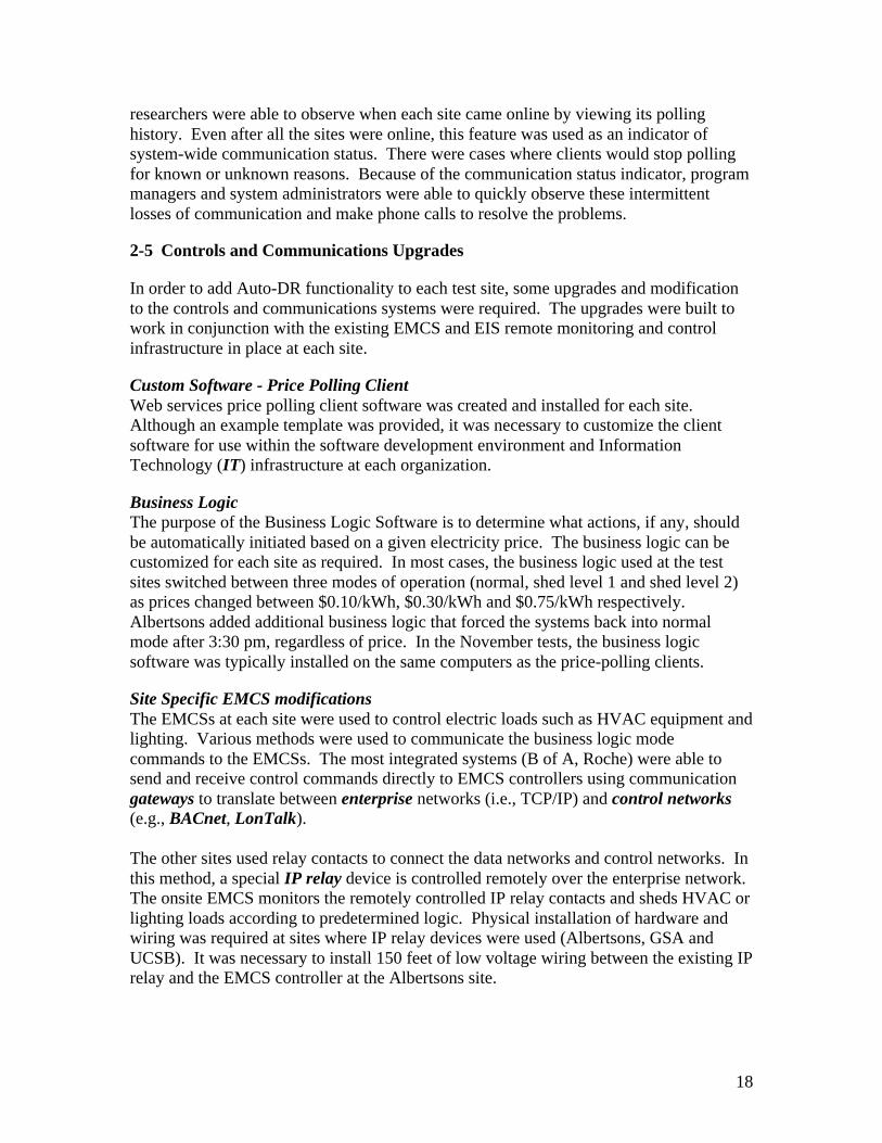
The actual signal sent on November 12th, 2003 is presented in Figure 2-8. This figurewas downloaded from the user interface of the price scheduling application. Theintention of the first test was to keep the signal as simple as possible but still test twolevels of response.
20
0
0.1
0.2
0.3
0.4
0.5
0.6
0.7
0.8
9:00
9:30
10:0
010
:30
11:0
011
:30
12:0
012
:30
13:0
013
:30
14:0
014
:30
15:0
015
:30
16:0
016
:30
17:0
017
:30
18:0
018
:30
19:0
019
:30
Pri
ce V
alu
e [$
/kW
h]
Figure 2-9. Test 1 Price Signal (November 12th, 2003)
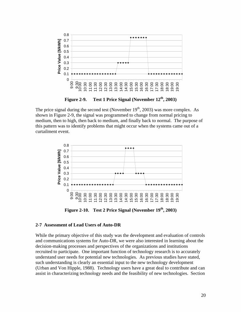
The price signal during the second test (November 19th, 2003) was more complex. Asshown in Figure 2-9, the signal was programmed to change from normal pricing tomedium, then to high, then back to medium, and finally back to normal. The purpose ofthis pattern was to identify problems that might occur when the systems came out of acurtailment event.
0
0.1
0.2
0.3
0.4
0.5
0.6
0.7
0.8
9:00
9:30
10:0
010
:30
11:0
011
:30
12:0
012
:30
13:0
013
:30
14:0
014
:30
15:0
015
:30
16:0
016
:30
17:0
017
:30
18:0
018
:30
19:0
019
:30
Pri
ce V
alu
e [$
/kW
h]
Figure 2-10. Test 2 Price Signal (November 19th, 2003)
2-7 Assessment of Lead Users of Auto-DR
While the primary objective of this study was the development and evaluation of controlsand communications systems for Auto-DR, we were also interested in learning about thedecision-making processes and perspectives of the organizations and institutionsrecruited to participate. One important function of technology research is to accuratelyunderstand user needs for potential new technologies. As previous studies have stated,such understanding is clearly an essential input to the new technology development(Urban and Von Hipple, 1988). Technology users have a great deal to contribute and canassist in characterizing technology needs and the feasibility of new technologies. Section

21
5 of this report discusses the lessons learned from using the Lead user concept inevaluating the needs and methods to promote DR in large facilities.
Lead users have been identified as an extremely valuable cluster of customers andpotential customers who can contribute to the identification of future opportunities andevaluation of emerging concepts. Lead users are defined as organizations that exhibit thefollowing two characteristics:
• They face the general marketplace needs months or years before the bulk of themarketplace encounters them.
• They are positioned to significantly benefit from obtaining solutions to thoseneeds.
The managers of these types of programs realize that the solutions to energy problems arebeyond the ability of one company or facility to solve. They are willing participants inthis research project primarily because they understand the problems that could occur iffacilities need to be shut down in an energy emergency. It was early in the developmentof an Auto-DR program for their facilities, but managers were willing to undergoextensive interviews and work together cooperatively with the research team to conductthe Auto-DR test and take part in the Lead Users evaluation.
The Lead User evaluation included a series of interviews with each of the key facilitymanagers and owners. These interviews took place during the recruitment process. TheAuto-DR organizational study methodology was primarily telephone interviews of theparticipants at the facility and the vendors who serve the facilities. The participants arelocated at some distance from each other and much of the work they do with the sites isvia telephone and email. Shockman et al (2004) describe the results of the organizationalinvestigation.

22
23
3. Auto-DR Systems Characterization and Measurement
In the Auto-DR test, each of the five participating sites used different approaches in thedesign and implementation of their systems. This section examines the generalcharacteristics of these systems. Where possible, metrics are used to quantify variousattributes and characteristics of the Auto-DR systems. Quantifiable Auto-DR metrics areshown in tables following each section.
3-1 Auto-DR System Architecture
An Overview
Some Auto-DR facilities hosted the polling client software on-site and others hosted it atremote co-location sites (see Table 3-1). The geographic location of the computer thathosts the polling client is less important than the type of environment where it is hosted.Professional co-location hosting services, or “co-los” offer highly secure environmentsfor hosting computers and servers. Co-los generally provide battery and generatorbacked electrical systems, controlled temperature and humidity, seismic upgrades and24/7 guarded access control. For companies that don’t have similarly equipped datacenters, co-los fill an important need. For computer applications where high availabilityis important, co-location facilities are often used.
Systems with a high level of integration between enterprise networks and EMCSnetworks tend to allow direct access to any or all control points in the EMCS withoutexcessively labor intensive point mapping required. Direct remote control of EMCSpoints from enterprise networks means that the business logic computer has the ability tosend commands over the network(s) that extend all the way to the EMCS I/O controllerconnected to the equipment that is shed. In a highly integrated system, the EMCSbecomes an extension of the enterprise. In these types of integrated systems, a gatewaydevice is used to translate between the different protocols used in enterprise networks andEMCS networks.
Alternately, some systems used relay contacts to interface between enterprise networksand EMCS networks. Relay contacts are commonly used in EMCS programming todefine mode changes (e.g., smoke detector contacts). However, the use of relay contactsas an interface between networks is not very flexible. Modifications to shed strategies orother types of remote control would be more difficult with a relay interface system thanwith an integrated system with a translating gateway. Both gateway based and relaybased interfaces to EMCSs can be effective for initiating shed strategies.

24
Table 3-3. Characteristics of Auto-DR Systems - ArchitectureAlbertsons B of A GSA Roche UCSB
Client hosted at co-lo Yes Yes No No NoRemote polling client Yes Yes Yes No NoRemote control viaInternet Gateway
No Yes No Yes No
Gateway TypeGateways used in building telemetry systems provide several functions. First, theyconnect two otherwise incompatible networks (i.e., networks with different protocols)and allow communications between them (see Figure 3-1). Second, they providetranslation and usually abstraction of messages passed between two networks. Third,they often provide other features such as data logging, and control and monitoring of I/Opoints.
Of the five Auto-DR sites, two used embedded two-way communicating gateways toconnect each site’s EMCS networks to its enterprise networks (Table 3-2). Embeddeddevices are generally preferred over PC based gateway solutions for scalable, ongoingsystem deployments. Embedded devices have the following advantages:
• More physically robust. There are no hard drives or other moving parts.• Less susceptible to viruses and other types of hacker attacks due to custom
designed operating systems and applications.• Less susceptible to human error. Once they are set up to function, there is no
reason for site personnel to interact with the device. Since they are not “generalpurpose” computers, there is no risk of memory overloads due to computergames, screen savers and other applications that may be inadvertently loaded ontothem.
• Better form factor. Embedded devices are usually smaller than PCs and aredesigned to be mounted in secure server rooms with other IT equipment.
• Lower cost. Although volume dependent, application specific embedded devicescan be produced in volume for lower cost than PCs.
At Albertsons, an embedded IP I/O device (Engage EPIM™) was used for powermonitoring and shed mode control. The EPIM provided power monitoring by directlycounting pulses from power meters. The EPIM set various shed modes into operation byopening and closing onboard relay contacts. Although the EPIM IP I/O deviceeffectively provides the interface between the EMCS and enterprise networks, it does notfit the most basic definition of a gateway. It does not connect the protocols of the twonetworks.
At UCSB, gateway functionality for monitoring was provided by software running on aPC. A previous version of gateway software also provided remote control functionality,but this feature was unavailable at the time of the Auto-DR test due to incompatibilityissues that occurred after a software upgrade. To meet the remote control requirements

25
of the Auto-DR test, an embedded IP I/O device was added. This device had onboardrelay contacts similar to the EPIM, but direct measurement of I/O points (such as powermeters) was not required.
Table 3-4. Characteristics of Auto-DR Systems - Gateways
Gateway typeInterface DeviceDescription for
Remote Shed Control
Remote MonitoringDescription
AlbertsonsEmbedded IP I/O
deviceIP Relay (2 contacts)
Meter pulses aremonitored through
gateway
B of A Embedded GatewayControl of EMCS via
Internet gatewayMonitoring of EMCS
through gateway
GSAEmbedded IP I/O
device IP Relay (2 contacts)None
Roche Embedded GatewayControl of EMCS via
Internet gatewayMonitoring of EMCS
through gateway
UCSB
PC based Gatewayfor monitoring,
Embedded IP relayfor control
IP Relay (3 contacts)
Selected EMCS pointsmonitored through
gateway
Figure 3-1, “Network architecture overview of five combined Auto-DR sites” shows thecommon source of electricity price and the communications protocol translations betweenthe business logic and the final control element (relays, valves etc.) controllers thatactually shed the electric loads. Gateways or other devices are used to transfer necessarycommunications between dissimilar network protocols.

26
Albertsons
(Internet) XML over SOAP, HTTP,
TCP/IP
Polling Client &
Business Logic
(Private WAN)
TCP/IP
IP I/O Relay
Lights, Heater
BofA
(Internet) XML over SOAP, HTTP,
TCP/IP
Polling Client &
Business Logic
(Private WAN)
TCP/IP Gateway Gateway
Fan Pressure
GSA
(Internet) XML over SOAP,
HTTP, TCP/IP
Polling Client &
Business Logic
(Private WAN)
TCP/IP Gateway
IP I/O Relay
Zone Temps
GatewayFans
On/Off
GatewayFans
On/Off
UCSB
(Internet) XML over SOAP,
HTTP, TCP/IP
Polling Client &
Business Logic
(Private WAN)
TCP/IP
IP I/O Relay
EMCS Protocol
#4Gateway
EMCS Protocol
#6Gateway
EMCS Protocol
#4
Fan Speed,
Valves etc.
EMCS Protocol #4
Polling Client &
Business Logic
Roche
(Internet) XML over SOAP, HTTP, TCP/IP
Price Server
($/kWh)
Original Site EMCS Architectures (circa 1999)Technology Added
for CEC Programs in 2001
Technology Added for Auto-DR Tests 2003
EMCS Protocol #1
EMCS Protocol #7
EMCS Protocol #2
(Private WAN)
TCP/IP
EMCS Protocol #5
EMCS Protocol #3
EMCS Protocol #3
Figure 3-11. Network architecture overview of five combined Auto-DR sites
IntegrationFor purposes of this study, integration between EMCS and EIS can be characterized byasking two key questions. First, can data from the EMCS and EIS be viewed andanalyzed from one Human Machine Interface (HMI)? Second, do the EMCS devicessuch as energy meters reside on the same network as the EMCS devices? Table 3-3summarizes the answers to these questions for each of the sites. Albertsons, B of A, andGSA either don’t have EIS or else they are not integrated with the EMCSs at those sites.At Roche, the Tridium system integrates most of the EMCS points and a smallpercentage of the electric meters into a comprehensive HMI for viewing, archiving andanalysis. UCSB has extensive monitoring of most of the electric meters and sub-metersthroughout the campus. Data from these meters are available for visualization, archivingand analysis through the SiE (Itron / Silicon Energy) server along with relevant EMCSpoints that have been mapped over to it. Electric meters do not reside on the samenetwork as the EMCS devices at either the Roche or UCSB sites.
One distinguishing characteristic of the Auto-DR sites was whether or not they leveragedthe existing corporate or campus enterprise network to transmit EMCS and/or EIS data.Use of the existing enterprise network for this purpose has many advantages. Systeminstallation costs can be much lower if existing enterprise networks are used forcommunications instead of installing new, separate networks solely for EMCSs and EISs.

27
In addition, the Information Technology department that manages the enterprise is oftenbetter equipped to assure network reliability and security than the facilities group thattraditionally maintains the EMCS and EIS.
Each facility has different functional requirements and organizational structures thatdictate how the enterprise, EMCS and EIS networks are designed, installed andmaintained. Of the five sites in the Auto-DR test, three of them shared mission criticalenterprise networks with EMCS/EIS/Auto-DR systems. Although bandwidthrequirements for EMCS/EIS/Auto-DR systems are not great, other organizationalimpediments prevent the sharing of enterprise networks for non-standard purposes.
At GSA, a completely separate enterprise network was created for the GEMnetEMCS/EIS/Auto-DR system. This was the logical choice for this facility because it wasnot practical to share the existing enterprise networks with other tenants at the site: theGovernment Services Administration (GSA) and the Federal Bureau of Investigation(FBI). In such circumstances, it is easier to create a new enterprise network for local andremote access to EMCS and EIS data than it is to resolve complex security andmaintenance issues associated sharing an enterprise network with another department ororganization.

28
Table 3-5. Characteristics of Auto-DR Systems - IntegrationAlbertsons B of A GSA Roche UCSB
Integrated EMCS & EIS No No No Partial PartialPrimary enterprise networkshared withEMCS/EIS/Auto-DRsystems
Yes Yes No Yes Partial
Shed Control CharacteristicsEach Auto-DR site used different shed strategies. The control characteristics of thesestrategies also varied substantially. This section describes the characteristics of each shedstrategy (Table 3-4). The number of shed control points is one characteristic of a givenAuto-DR implementation. It represents the quantity of points that were adjusted oraltered to invoke the shed strategy at each site. Shed control points include hardwarecontrol points (for example, valve position) and software points (for example, setpoints)that were altered during the shed. Software points other than setpoints were not included.Control granularity and closed loop shed control are both factors that influence thelikelihood and degree to which some occupants may be negatively affected by the shedstrategy.
Albertsons had only two control points (overhead lights & anti-sweat heaters). Becausethe size of the store is comparatively small, this was rated as “medium” controlgranularity. Switching off half of the overhead lights is an open loop type of control (i.e.,there is no feedback to the system). The anti-sweat heater remained in closed loopcontrol during the shed by operating with a reduced setpoint.
B of A had just one control point (duct static pressure) for the entire 211,000 ft2 building,hence the “coarse” control granularity rating. The shed strategy of resetting the ductstatic pressure so as to maintain zone temperature is a type of closed loop control, but thedearth of temperature sensors in the zones reduced the closed loop rating to “partial”.
In stark contrast to the rest of the sites, the GSA building used a fine granularity, closed-loop shed control strategy. The zone temperature setpoints for each of 1,050 VAVterminal boxes (1,400 including reheat side of dual duct boxes) were “relaxed” during theshed. In other words, the cooling setpoints were raised and the heating setpoints werelowered. This approach had an energy saving effect on the central HVAC systems whileassuring a known level of service modification to the occupants.
The Roche site used a coarse open loop shed strategy of shutting off fans during the shed.
UCSB used a variety of shed strategies of medium granularity. The shed strategies(including closing cooling valves, and reducing duct static pressure) were all open loop.The outside air dampers were opened to 100%, a strategy that could backfire in extremelyhot conditions. The temperate climate in Santa Barbara made this scenario unlikely.

29
Table 3-6. Characteristics of Auto-DR Systems - Shed ControlAlbertsons B of A GSA Roche UCSB
Number ofShed Control Points 2 1 ~ 1,400 7 42
Shed ControlPoints per 10,000 ft.2 0.4 0.05 14 0.4 1.4
Control Granularity Medium Coarse Very Fine Medium FineClosed loop shedControl Partial Partial Yes No No
Open StandardsIn the EMCS and EIS fields, protocols refer to the low-level communication languagesthat devices use to “talk” to one another on the network. Of course, one device can onlytalk to another if they are speaking the same language. Traditionally, each control systemmanufacturer built controllers and other devices that only spoke their own unpublishedproprietary protocol (Table 3-5). Once a system is built using a proprietary protocol, theoriginal manufacturer or their representatives are the only parties that can makesubstantial additions or changes to the system. Some control companies use proprietaryprotocols as a “lock” on their customers’ systems so as to ensure future business and highprofit margins.
Over the past fifteen years or so, there has been a movement toward “open” protocols inthe EMCS and EIS industries. Open protocols are based on published standards open tothe public. Interested companies can build products that communicate using openstandards. In a truly open, interoperable system, products from a variety of open productvendors could be added at any time by skilled installers from independent companies.Several sites in the Auto-DR test use open EMCS and/or EIS products that include theBACnet, LonTalk (EIA-709) and Modbus open protocols.
Even with considerable interest from building owners few, if any, new or existingbuilding EMCS or EIS systems are truly open and interoperable. Even when openprotocols are used, they are often installed as part of a system that requires use ofproprietary software or components at the higher levels of the system architecture.Another way “openness” is reduced is by designing products and systems that requireproprietary software tools for installation.
In the IT marketplace, open protocols (e.g., TCP/IP), open database interface standards(e.g., ODBC) and open hardware standards (e.g., SIMM) have helped the industry thrive.This has allowed products from a wide variety of vendors to communicate with oneanother on internal LANs, WANs and the Internet. A service industry of independentSystems Integrators has grown to fill the need of integrating multiple vendor networksinto cohesive systems.
Another important trend in the IT industry is the use of a new set of open standards,protocols and languages collectively known as XML/ Web services. The use ofXML/Web services in the building controls industry is increasing. This trend will tend to
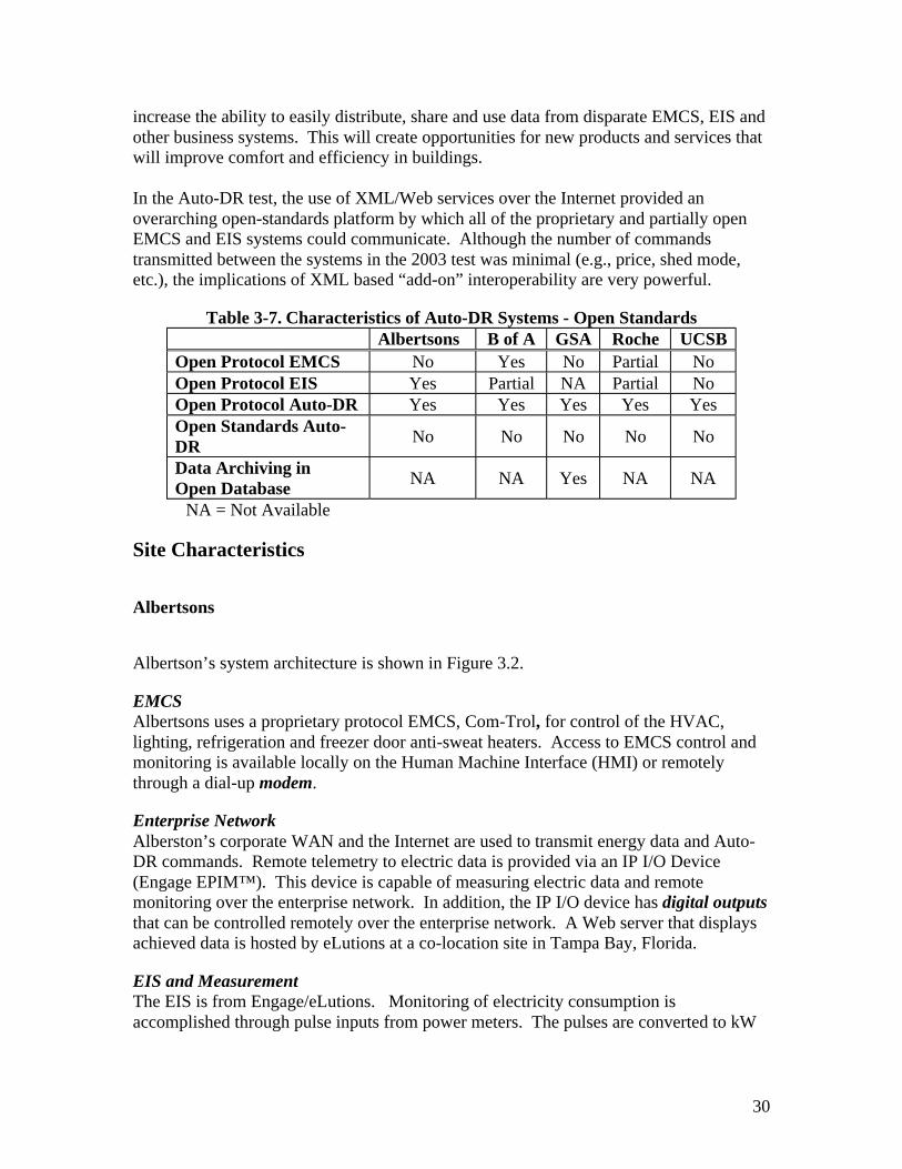
30
increase the ability to easily distribute, share and use data from disparate EMCS, EIS andother business systems. This will create opportunities for new products and services thatwill improve comfort and efficiency in buildings.
In the Auto-DR test, the use of XML/Web services over the Internet provided anoverarching open-standards platform by which all of the proprietary and partially openEMCS and EIS systems could communicate. Although the number of commandstransmitted between the systems in the 2003 test was minimal (e.g., price, shed mode,etc.), the implications of XML based “add-on” interoperability are very powerful.
Table 3-7. Characteristics of Auto-DR Systems - Open StandardsAlbertsons B of A GSA Roche UCSB
Open Protocol EMCS No Yes No Partial NoOpen Protocol EIS Yes Partial NA Partial NoOpen Protocol Auto-DR Yes Yes Yes Yes YesOpen Standards Auto-DR
No No No No No
Data Archiving inOpen Database
NA NA Yes NA NA
NA = Not Available
Site Characteristics
Albertsons
Albertson’s system architecture is shown in Figure 3.2.
EMCSAlbertsons uses a proprietary protocol EMCS, Com-Trol, for control of the HVAC,lighting, refrigeration and freezer door anti-sweat heaters. Access to EMCS control andmonitoring is available locally on the Human Machine Interface (HMI) or remotelythrough a dial-up modem.
Enterprise NetworkAlberston’s corporate WAN and the Internet are used to transmit energy data and Auto-DR commands. Remote telemetry to electric data is provided via an IP I/O Device(Engage EPIM™). This device is capable of measuring electric data and remotemonitoring over the enterprise network. In addition, the IP I/O device has digital outputsthat can be controlled remotely over the enterprise network. A Web server that displaysachieved data is hosted by eLutions at a co-location site in Tampa Bay, Florida.
EIS and MeasurementThe EIS is from Engage/eLutions. Monitoring of electricity consumption isaccomplished through pulse inputs from power meters. The pulses are converted to kW

31
demand in the IP I/O device and accessed remotely through the eLutions Web basedmonitoring system. The Engage/eLutions EIS provides the following features:
• Monitoring: whole building and panel sub-metering.• Visualization: Graphical charts including time-series, daily/monthly consumption
summary, calendar profile, 3D profile, and duration curves.• Data Archive: minute interval electric data are downloadable via the website.• Other: The energy manager can select multiple Albertson sites and compare/rank
their energy usages, though only one Albertsons site is featured in this test.
Auto-DR System DescriptionThe computer containing the Auto-DR polling client and business logic is hosted atElusion’s co-lo in Florida. The business logic determines the correct operational modefor the Oakland store at any given time (normal, shed level 1, shed level 2) based on priceand other operational criteria. It commands the IP I/O device relays to open or closeusing a predetermined code that represents each operational mode. These relay contactsare monitored by the Com-Trol EMCS. Upon sensing the state of the relay contacts, theEMCS commands the overhead store lights and anti-sweat heaters according to the shedstrategy. The following business logic was essential at this site. As the store manager’spreferred to return the store to normal operation by the evening shopping rush, all storesystems are forced to “normal” operation between 3:30 pm and 10:00 pm, regardless ofthe current price of electricity.
Shed StrategyIn normal mode, the overhead lights are all on (100%) during occupied hours. Thefreezer door anti-sweat heaters are controlled so as to prevent the glass doors fromfogging when opened. The anti-sweat heaters control system uses a pulse widthmodulation (PWM) scheme that controls the amount of heat supplied to the glass basedon the measured dewpoint temperature in the store. At night the dewpoint temperaturesetpoint is changed so as to use less energy. Upon a rise in price to $0.30/kWh, overheadlighting was reduced by 50% by switching off half of the fluorescent tubes in eachfixture. Upon a rise in price to $0.75/kWh, the anti-sweat freezer door heater controlswitched to “night mode” which uses significantly less energy.

32
Internet
Infotility Price Server
LBNL Price Scheduler
Polling Client& Business LogiceLutions - Florida
Albertson'sCorporate WAN PSTN
EPIM tm
IP I/ODevice
EMCSController
WholeBldg.PowerMeter
OverheadLighting Panel
Freezer DoorAnti-Sweat
Heater Panel
Freezer CaseLighting Panel
Modem
Pro-prietary
EMCSController
L
Shed ControlMonitoring
Shed ControlDisabled
FreezerCase Lights
ChickenCooker
Freezer DoorAnti-Sweat Heaters
Overhead Lights 50%
Albertson's Store 7049Oakland, CA
Remote EMCS HMI
Modem
150' Shed ControlWiring (added)
HVAC Control
Figure 3-12. Albertsons – System Architecture

33
Bank of America Concord Technology Center (CTC)
Bank of America’s Concord Technology Center (CTC) system architecture is shown inFigure 3.3.
EMCSThe B of A CTC buildings involved in the Auto-DR test use an open protocol (LonTalk)system by Trane for control and monitoring of the HVAC equipment. Inter-buildingconnectivity is accomplished through use of another open protocol (BACnet).
Enterprise NetworkB of A uses the corporate WAN and the Internet for remote telemetry to the EMCS andEIS. Connectivity between the enterprise networks and the EMCS networks is providedby Tridium JACE™ gateways. The gateways connect the BACnet EMCS (includingelectric meters) to the B of A enterprise WAN. The EMCS, EIS and Auto-DR data aretransferred across the same enterprise network infrastructure used for bank financialtransactions. At the B of A Network Operations Center (NOC) in Chicago,communications between the B of A WAN and the WebGen Polling Client / Businesslogic computer in Andover MA is established across the public Internet. Cisco VirtualPrivate Network (VPN) routers were used at both ends of the secure VPN “tunnel”.WebGen also provided a Web server, hosted at the co-location site in Andover,Massachusetts, for visualization of the EMCS and EIS data.
EIS and MeasurementFor the Auto-DR test, monitoring, archiving and visualization of energy data wereaccomplished through the use of three separate systems: PG&E (Interact), WebGen(IUE), and temporary sub-metering equipment.
InterAct is a Web based, whole site EIS provided by PG&E for large commercialcustomers. At the B of A CTC, site demand, individual building interval data, andweather data from NOAA can be monitored and trended. The data can be visualized inthe following formats: Time-series, daily/monthly consumption summary, scatter plot,histogram and average daily profile. IUE’s features include control, monitoring and datavisualization. The control characteristics implemented for the Auto-DR test are describedbelow. This system is also described in Motegi et al, 2003a. Since the existing site EISsystems did not measure electric data at the level of resolution required for the Auto-DRtest, additional temporary sub-metering equipment was added.
Auto-DR System DescriptionWebGen system is designed to operate as an ongoing demand and energy reductionsystem. To save energy, the WebGen IUE system intermittently takes setpoint controlaway from local operators and gives control to the automated system in Andover. Duringthese “interventions”, duct static pressure setpoint is reduced on one VAV fan system at atime. The setpoint reduction was rotated between fans so as to share the reduction isservice throughout the site.

34
The computer containing the Auto-DR polling client and business logic was hosted atWebGen’s co-lo in Andover, MA. The business logic contains learning algorithmsdesigned to maintain comfort while reducing energy costs. The Auto-DR price signalwas intended to further reduce energy use.
WebGen has a unique feature that estimates the savings (dollars and kWh) that arerealized each time the WebGen system causes control to vary from normal operation. Atthe B of A CTC site, sensors are not installed for fan power, fan airflow, or pressure dropacross fans. Since data necessary to calculate the energy savings per intervention are notmeasured at this site, it is not possible for the WebGen system to make accurate estimateson a “per intervention” basis.
WebGen’s site wide financial savings calculations are made using revenue grade electricmeters. Savings are calculated as the difference between the measured whole site electricmeter values (with shed interventions) and what the electric consumption “would havebeen” without the sheds. These calculations may be accurate within the constraints ofnormal regression analysis based on current standards of practice such as those used inthe International Performance Measurement and Verification Protocol (IPMVP).
Shed StrategyAs fan duct static pressure setpoints are reduced to save fan energy, sensor data(temperatures, pressures, etc.) are evaluated. The system is designed to “learn” the effectreductions in the duct static pressure has on zone temperatures so as to minimize negativecomfort impacts. Artificial Intelligence algorithms are used in these calculations. Duringthe Auto-DR test, the system responded by reducing duct static pressure by 0.2” W.C. for20 minutes per fan. Pressure reductions were rotated between fans in different buildingsto maintain comfort and shed demand at the same time.
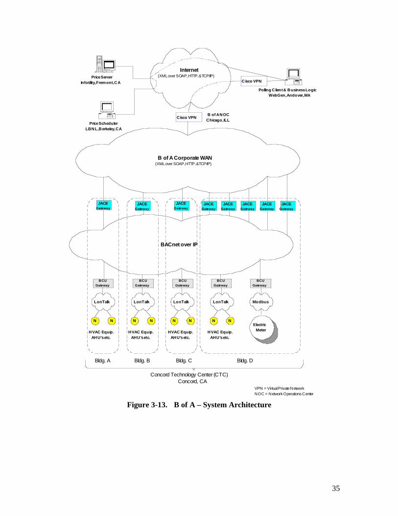
35
Price ServerInfotility, Fremont, CA
Price SchedulerLBNL, Berkeley, CA
Polling C lient & Business LogicWebGen, Andover, MA
Cisco VPN
Cisco VPN
B of A Corporate WAN(XML over SOAP, HTTP, &TCP/IP)
BACnet over IP
JACEGateway
JACEGateway
JACEGateway
JACEGateway
JACEGateway
JACEGateway
JACEGateway
JACEGateway
LonTalk
N N
LonTalk
N N
LonTalk
N N
LonTalk
N NElectric
Meter
Modbus
HVAC Equip.AHU's etc.
HVAC Equip.AHU's etc.
HVAC Equip.AHU's etc.
HVAC Equip.AHU's etc.
Bldg. A Bldg. B Bldg. C Bldg. D
Concord Technology Center (CTC)Concord, CA
Internet(XML over SOAP, HTTP, &TCP/IP)
B of A NOCChicago, ILL
VPN = Virtual Private NetworkNOC = Network Operations Center
BCUGateway
BCUGateway
BCUGateway
BCUGateway
BCUGateway
Figure 3-13. B of A – System Architecture
36
General Services Administration – Oakland Federal Building, Oakland
The Oakland Federal Building system architecture is shown in Figure 3.4.
EMCSA Johnson Metasys proprietary protocol EMCS is used to control the VAV fan systemand central heating and cooling plants. Although they are not used for HVAC control,several Alerton BACnet open protocol devices were used to facilitate Auto-DRcommunications.
Enterprise NetworkThe Oakland GSA site is connected to an innovative enterprise network designed toimprove the efficiency and operations of the connected buildings. GEMnet (GSA Energyand Maintenance Network) is being developed and implemented for energy managementand building maintenance in over a dozen Federal buildings in the Pacific Rim Region.The enterprise network and DSL Internet connectivity were designed and implementedby controls and IT specialists within the facilities group of GSA.
EIS and MeasurementMonitoring, archiving and visualization of energy data were accomplished through theuse of three separate systems: PG&E (Interact), EMCS trend logs, and temporary sub-metering. The Interact system monitors five interval meters throughout the building thatcollectively measured whole building demand and energy. Temporary sub-metering wasadded to this site to monitor four cold deck supply fans and two secondary chilled waterpumps.
Auto-DR System DescriptionIn the Auto-DR test, a polling client in Kelowna, British Columbia (BC) polled theInfotility price server in Fremont. Upon a rise in price, the business logic in the BCcomputer posted a value that represented shed mode (normal, shed level 1, shed level 2)to the main GEMnet SQL database. A custom software application called BACnet readerpolled the SQL database every 2 minutes. When the mode value changed to a shedmode, BACnet reader commanded an Alerton I/O controller with 2 digital outputs (via asoftware gateway by PolarSoft and an Alerton LSI TCP/IP to BACnet MSTP gateway) toclose either one or two relay contacts. An I/O controller with two digital inputs read therelay contacts. The shed strategy was then implemented throughout the Johnson EMCS.
Shed StrategyGSA employed a global zone temperature setpoint setup/setback shed strategy (Figure 3-6). Upon commencement of a shed (due to price increase), the zone temperaturesetpoints for all of the individual zones in the building were “relaxed”. In other words, iffan and cooling energy is being used to keep a given zone from rising above 74°F, a newsetpoint is issued to keep it from rising above 76°F. Similarly, zones that have heatingsetpoints are relaxed to allow zones to get slightly cooler before using more energy.When this approach is applied to all of the zones in the building, substantial energy canbe saved.

37
Table 3-8. Oakland GSA Zone Temperature Setpoints - Normal and Shed Modes
Shed ModeZone Heating
Setpoint Zone Cooling Setpoint
Normal 70°F 72°FLevel 1
($0.30/kWh) 68°F 76°F
Level 2($0.75/kWh) 66°F 78°F

38
Proprietary(Johnson)
Price ServerInfotility, Fremont, CA
Price SchedulerLBNL, Berkeley, CA
Polling Client& Business Logic
Vancouver, BC
GEMnetSQL Database
GEMnetOakland(TCP/IP)
BACnetMSTP
Internet
DSL DSL
BACnet Reader
GTWY1
C1
C2
C2
C2
C2
C2
C2
C2
GSA - Oakland, CA 450 Golden Gate, SF, CA
WebCNTL TM
ALC EMCSWeb Server
C1
C1
C1
BACnetMSTP
C3
C3
C1
C1
C3
GEMnet, S.F.(TCP/IP)
BrowserBrowser
C3 = ALC ControllerGTWY2 = ALC LGE GatewayC1 = Alerton ControllerC1 = Alerton VLC Controller
C2 = Johnson ControllerGTWY1 = Alerton LSI Gateway
Polling Client polls price server andposts latest price to GEMnet SQLdatabase. BACnet reader readsdatabase every 2 min. and controls VLCrelays to switch EMCS to appropriatecontrol mode to shed electric loads upona rise in price.
GTWY2
Figure 3-14. GSA Oakland – System Architecture
39
Roche Pharmaceuticals Palo Alto
The Roche Pharmaceuticals system architecture is shown in Figure 3.5.
EMCSThe EMCS at the Roche site is comprised primarily of Invensys products. There are atleast two generations of Invensys products used: Network 8000 (proprietary protocolRS-485) and the I/A product line (open protocol LonTalk). In addition, open protocolModbus and proprietary RS-485 (different from the Network 8000) are used forelectricity monitoring. These diverse systems are tied together into one common userinterface and database by the Tridium Niagra framework. The Tridium system usesembedded gateways to translate from each aforementioned EMCS protocol to TCP/IP.
Enterprise NetworkThe Tridium system provides password-protected access of the EMCS data via any Webbrowser within the Roche corporate intranet. Due to security concerns and lack ofcompelling reason to do otherwise, the Tridium EMCS/EIS Web browser is notaccessible from the public Internet.
Due to security concerns, the polling client was installed just outside of the Roche secureintranet in a DMZ region8. A special virtual connection was made between the Tridiumcomputer inside the secure Roche intranet and the polling client computer that is locatedin the DMZ. This allows the polling client easy, two-way communication with othercomputers in the public Internet, while not exposing the Roche network to securityconcerns associated with the Internet.
The polling client computer also served another purpose. To aid in the data collectionrequirements of the Auto-DR project, about 40 EMCS points were extracted from theTridium system and logged and archived on a computer outside of the Roche securenetwork. These data were made available to LBNL researchers in Berkeley in near realtime.
EIS and MeasurementMonitoring, archiving and visualization of energy data were accomplished through theuse of three separate systems: Tridium (Vykon™), Pegasys (PML™), Infotility Real-Time Energy Tracker (RTET). Tridium Vykon provided Internet based control andtrending for Roche inside their firewall. RTET is a real-time Infotility Web-monitoringtool designed specifically for this project. It was developed to overcome the remote dataaccess problems related to Roche’s Internet firewall. RTET was used to transmit energydata from the Tridium computer to the Infotility server where it could be accessedremotely by project researchers. The Pegasys system provided electricity, gas, steam andwater metering. It was used to obtain data for three buildings (A2, SS and FS). ThePEGASYS PML is a closed-network system that is only accessible within the site.
8 “Short for demilitarized zone, a computer or small subnetwork that sits between a trusted internalnetwork, such as a corporate private LAN, and an untrusted external network, such as the public internet”,Webopedia. 2004. http://www.webopedia.com/TERM/D/DMZ.html. Viewed on Mar. 15, 2004 .

40
Considerable effort was required to determine how to download and analyze the PML™data.
Auto-DR System DescriptionNo extra hardware was required to enable the Roche site’s Auto-DR functionality.Communication from the price server to the EMCS I/O controllers occurred vianetworks. The increased price was sensed by the polling client and passed through to theTridium system where it was read by the EMCS.
Shed StrategyThe shed strategy implemented at Roche is simple: when the price rises to $0.30/kWh,several constant volume fans are shut off. When the price rises to $0.75/kWh severalmore fans were turned off. This strategy was very effective at immediately reducingelectric load. It is also a rather severe measure to impose upon occupied areas, especiallyin hot weather. For the Auto-DR test, the fans that were selected for shedding and thestrategy employed were carefully selected by building operators to minimize adverseeffects on occupants.
The fan systems serving the selected areas have dual supply fans that operate in parallel.The return fan systems have a similar dual fan configuration. During the shed, only oneof the fans in each parallel system was disabled. Because of this, about half of thenormal air supply continued to flow into the buildings while the shed was in effect.
The fans involved in the shed serve the cafeteria. Since the test was conducted in themid-afternoon, the lunchtime crowd was gone and the cafeteria had very few occupants.Similarly the facility’s office and administration auditorium had low occupancy duringthe test. Zone temperature and system CO2 sensors indicate that there was a minimalimpact on the comfort of the areas affected by the shed. Temperature did not measurablydeviate from setpoint and CO2 level decreased during the shed.
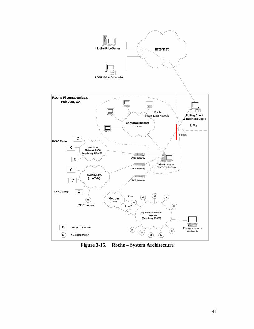
41
Internet
Corporate Intranet(TCP/IP)
InvensysNetwork 8000
Proprietary RS-485
Invensys I/A(LonTalk)
Modbus(TCP/IP)
Pegasys Electric MeterNetwork
(Proprietary RS-485)
Infotility Price Server
LBNL Price Scheduler
Polling Client& Business Logic
Tridium - Niagra
JACE Gateway
JACE Gateway
JACE Gateway
M
M
MM
MM
M M
M
M
MM
C
C
C
C
C
C
DMZ
Line 1
Line 2"S" Complex
HVAC Equip
Firewall
RocheSecure Data Network
HVAC Equip
Roche PharmaceuticalsPalo Alto, CA
Energy MonitoringWorkstation
EMCS Web Server
C
M
= HVAC Controller
= Electric Meter
Figure 3-15. Roche – System Architecture
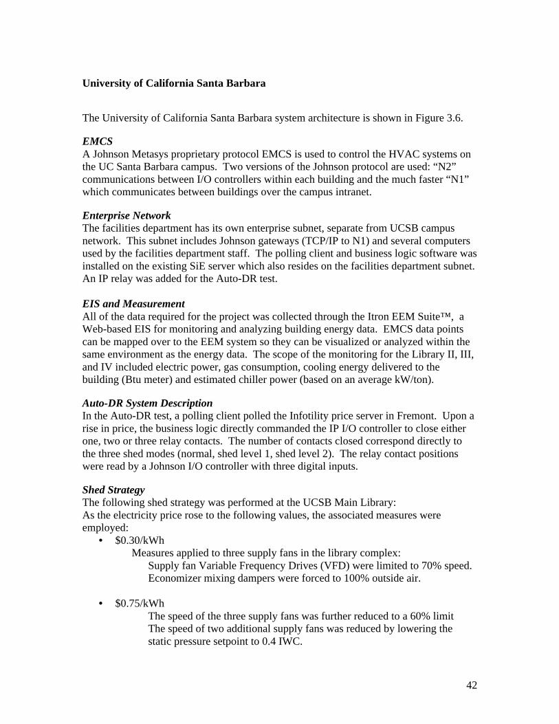
42
University of California Santa Barbara
The University of California Santa Barbara system architecture is shown in Figure 3.6.
EMCSA Johnson Metasys proprietary protocol EMCS is used to control the HVAC systems onthe UC Santa Barbara campus. Two versions of the Johnson protocol are used: “N2”communications between I/O controllers within each building and the much faster “N1”which communicates between buildings over the campus intranet.
Enterprise NetworkThe facilities department has its own enterprise subnet, separate from UCSB campusnetwork. This subnet includes Johnson gateways (TCP/IP to N1) and several computersused by the facilities department staff. The polling client and business logic software wasinstalled on the existing SiE server which also resides on the facilities department subnet.An IP relay was added for the Auto-DR test.
EIS and MeasurementAll of the data required for the project was collected through the Itron EEM Suite™, aWeb-based EIS for monitoring and analyzing building energy data. EMCS data pointscan be mapped over to the EEM system so they can be visualized or analyzed within thesame environment as the energy data. The scope of the monitoring for the Library II, III,and IV included electric power, gas consumption, cooling energy delivered to thebuilding (Btu meter) and estimated chiller power (based on an average kW/ton).
Auto-DR System DescriptionIn the Auto-DR test, a polling client polled the Infotility price server in Fremont. Upon arise in price, the business logic directly commanded the IP I/O controller to close eitherone, two or three relay contacts. The number of contacts closed correspond directly tothe three shed modes (normal, shed level 1, shed level 2). The relay contact positionswere read by a Johnson I/O controller with three digital inputs.
Shed StrategyThe following shed strategy was performed at the UCSB Main Library:As the electricity price rose to the following values, the associated measures wereemployed:
• $0.30/kWh Measures applied to three supply fans in the library complex:
Supply fan Variable Frequency Drives (VFD) were limited to 70% speed. Economizer mixing dampers were forced to 100% outside air.
• $0.75/kWh The speed of the three supply fans was further reduced to a 60% limit The speed of two additional supply fans was reduced by lowering the
static pressure setpoint to 0.4 IWC.

43
Economizer mixing dampers were forced to 100% outside air. The heating and cooling valves of all five fans were forced to 0% (closed).
Internet(XML over SOAP, HTTP, &TCP/IP)
Johnson N2Network
(Proprietary RS-485)
Price ServerInfotility, Fremont, CA
Price Scheduler
LBNL, Berkeley, CA
Polling Client& Business Logic
HVAC Equip
UCSBSanta Barbara, CA
Johnson N1 Network(Proprietary protocol over
TCP/IP)C
GTWY
GTWY
GTWY
GTWY
Johnson N2Network
(Proprietary RS-485)
Johnson N2Network
(Proprietary RS-485)
Johnson N2Network
(Proprietary RS-485)
C
C
C
CC
C
C
CC
C
C
IP I/O Device
(3) DI
PC w/ Gateway S/W
SiE Server
Firewall
LibraryOther Bldgs (typ)
Campus Data Network(TCP/IP)
RS-232
Fan VFD
Economizer Dmpr
CHW Valves
Facilities Bldg.
C = Johnson HVAC controller
GTWY = Johnson NetworkControl Module / Gateway
RLY1 RLY2 RLY3 MODE
ON Off Off NormalOff ON Off Shed 1Off Off ON Shed 2
Relay Logic for Shedding
Polling Client PC commands
IP I/O device relays uponincrease in price.
Figure 3-16. UCSB – System Architecture

44
3-2 Site Measurement and Evaluation Techniques
This section describes the site measurement and evaluation techniques used to measurethe electric demand shed. Measurement techniques were developed to evaluate each 15-minute increment of the three-hour electric shed event. Where possible, we alsodeveloped non-energy measurements focusing on temperature or other indoor airenvironmental factors (see Section 4). The shed events were followed by interviews withfacility operators to inquire about any loss of service or problem that may have resultedfrom the shed strategy (See Section 4 and Appendix V).
Numerous sources of data were used to measure and evaluate the load shedding. Table 3-7 summarizes the measurements at each site, showing the type of system, types of datacollected, number of data points used from the system, frequency of data measurement,and whether it had Web-based data access. Detailed point lists are included in AppendixVI. All five sites had some form of an EIS. Multiple sources of data including EIS,EMCS, and submeter were used in four of the five sites. At Albertsons, only one EISwas used for data collection and analysis. At the four sites with multiple sources of data,significant re-configuration of the EMCS and EIS trending points was required.
Table 3-9. Measurement Summary
Site Type Data type# of points
usedDatafreq.
Web-basedaccess
Albertsons
EISWBP, Overhead lighting,Anti-sweat heaters, OAT
4 15 min. Yes
EISWBP, Fan (status, temp, VFD,air flow, static pressure)
35 5 min. Yes
EIS WBP, OAT 2 15 min. Yes
EMCSChiller power, Chilled water energyControl status
21 15 min. No*B of A
SubmeterMeter installed: Fan power,Individual building power
8 1 min. No
EIS WBP, OAT 6 15 min. Yes
EMCS
WBP, Chiller power/energyFan (status, temp, VFD, air flow,static pressure)Cooling tower, Pump (status,VFD)Zone temp
1005-15min.
NoGSA
SubmeterMeter installed:Fan power, Pump power
6 1 min. No
EIS/EMCSNewly trended EMCS points:Fan status, Zone temp, CO2
19 5 min. Yes
EIS Individual building power 3 15 min. NoRoche
Submeter Spot measurement: Fan power No
EIS
WBP, Chilled water energy, OATNewly trended EMCS points:Fan power, VFD, static pressureEconomizer position, Zone tempCooling and heating valve position
1505-15min.
YesUCSB
EMCS Trends through EIS No

45
WBP – whole building power; OAT – outside air temperature; VFD – variable frequency drive;CO2 – carbon dioxide * Web access was not available to LBNL because of firewall security.

46
Demand savings were derived by subtracting the actual metered electric consumptionfrom the baseline consumption. The baseline consumption is an estimate of how muchelectricity would have been used without the demand shedding. We developed severalmethods to estimate baseline electricity consumption. Each building was evaluated usingtwo methods: 1) a whole building, or top-down, and 2) a component level, or bottom-upmethod.
Whole-Building Level Method
The whole building, or premise-level, top-down, analysis method consists of developinga whole-building electrical power baseline load shape. Whole building power isestimated using a weather regression model that assumes whole building power islinearly correlated with outside air temperature (OAT). The OAT data is from localweather stations. Input data are 15-minute interval whole building demand and hourlyOAT. This method was derived from previous work at LBNL (see KEMA-Xenergy,2003). In the previous work, this method was tested with the GSA data, and statisticallyproven to be a better estimate than the conventional method of simple averages9 when theWBP has a linear correlation with OAT. The model is computed as;
L15min = a15min + b15min Th
where L15min is the predicted 15-minute interval electric demand from the previous non-controlled working days. The number of previous days used in the model was selected tomake the best use of available metered data. Depending on frequency of availableweather data, Th is the hourly or 15-minute interval OAT. a15min and b15min are estimatedparameters generated from a linear regression of the input data. Separate regressionequations are developed for each 15-minute interval, resulting in 96 regressions for theentire day (24 hours/day, with four 15-minute periods per hour). An example of the OATlinear regression model is given in Appendix II.
To develop the baseline electric loads for the demand sheds we selected 18 “non-shed”days. These 18 baseline days were non-weekend, Monday through Thursday workdays.Fridays were eliminated in the development of the baseline because the UCSB Libraryhas a different operating schedule on Fridays. The selection of the baseline days wasbased on availability of whole-building data at each site. The submetering for Building Bat Bank of America was installed on October 15th, which was the first day of the 18-daybaseline period. The November 11th Veterans Day holiday was not included in thebaseline.
Figure 3-7 shows an example of the whole-building level baseline time-series chart onthe second test day (GSA). The chart shows whole building power for the shed (thelower curve) and the whole-building baseline power predicted if the shed had notoccurred. The vertical line at each baseline power data point is the standard error of the
9 California Independent System Operator (Cal ISO)’s Demand Response Program used “previous 10business days baseline”, which is a simple average of previous days.

47
regression estimate. The vertical lines at 1:15 pm, 2:15 pm, 3:15 pm, and 4:15 pmidentifies time intervals during which price signals were different.
0
500
1000
1500
2000
2500
3000
0:00
1:00
2:00 3:00
4:00
5:00
6:00
7:00
8:00
9:00
10:0
0
11:0
0
12:0
0
13:0
0
14:0
0
15:0
0
16:0
0
17:0
0
18:0
0
19:0
0
20:0
0
21:0
0
22:0
0
23:0
0
Who
le B
uild
ing
Pow
er [k
W]
Actual Whole-Building Method Baseline
Figure 3-17. Example of Whole-Building Method Baseline
Component Level Method
The component level, or bottom-up evaluation method develops the WBP savings bycombining the demand savings estimates for each component. The basic procedure is to:1) develop a baseline for each controllable component, 2) estimate the demand savingsfor the component by subtracting actual demand from the baseline, and 3) sum all thecontrollable load demand savings. The component level estimation method requiresanalysis of either direct power measurement or operational data for each controllablecomponent. The component level method is more accurate than the whole-buildingmethod if the controllable load and non-controllable load can be accurately measured.We developed several methods to develop the component level baseline load shape.These methods are described below.
Equipment Schedule MethodThe controllable component “normal-day” operational load shapes can be used to definea baseline if the equipment schedule is well defined and consistent. This method can beapplied to components with simple operational modes. This method is very accurate ifthe operation is simple enough to extrapolate electricity demand. A weather-sensitivecomponent load can not be evaluated using this method. Examples of components thatcan be evaluated using this method include constant volume fans operating with a fixedschedule and non-dimmable lighting.
Outside Air Temperature Regression Model MethodIf the component’s electricity demand is weather sensitive, a simple average of theprevious days’ demand may provide a lower baseline demand if the controlled day’stemperature is higher than that of the previous days. In this case, the estimate can beadjusted for OAT. This method forecasts the component demand by a regression modelsimilar to the whole-building level method. The 15-minute component electric demand

48
plus hourly OAT data are used. Examples of components evaluated with this methodinclude chillers and fans with VFDs.
Prior Time Load MethodIf the results of the equipment schedule or outside air temperature regression modelmethods do not accurately fit the actual demand data, the forecast demand may beestimated from the data at 15-minute to a few hours immediately preceding the test. Thisis a rule-of-thumb method. This method may be applied only when the equipmentoperation is stable without the shed strategies, and the daily load shape is similar over theprevious days. Depending on the demand profile, the calculation method can be selectedfrom either using previous operation hours or previous 15-minute demand, or drawing aline from the pre-shed demand and the post-shed demand. This method should be usedwhen the shed period is short, and there is no shed strategy applied in advance (such aspre-cooling).
Table 3-8 summarizes the component-level savings estimation methods used for differentcomponents at each site. There are various reasons why different evaluation methodswere used for the same type of equipment at different sites, due to load shapes andavailable data at each site.
Table 3-10. Component Level Methods for Each Component
Site ComponentEquipmentSchedule
OATRegression
Prior TimeLoad
Sales lightingsAlbertsons
Anti-sweat heaterB of A Fan system
FansChillersPumps
GSAOakland
Cooling towersRoche Fans
FansUCSB
Chillers
Figure 3-8 shows a component level method baseline time-series chart from the Rochesite. The chart shows the fan energy, total building energy and component savings.

49
0
100
200
300
400
500
600
700
800
0:00
1:00
2:00 3:00
4:00
5:00
6:00
7:00
8:00
9:00
10:0
0
11:0
0
12:0
0
13:0
0
14:0
0
15:0
0
16:0
0
17:0
0
18:0
0
19:0
0
20:0
0
21:0
0
22:0
0
23:0
0
Po
wer
[kW
]
Savings Others Fans
Figure 3-18. Example of Component Method Baseline - Roche

50
4. Results
This section discusses the results of the Auto-DR tests, including: discussions regardingthe receipt and confirmation of the XML price signal; discussion of the demand sheddingmeasurements; and non-energy measurements.
4-1 Requesting and Confirming Receipt of Signal
Infotility developed a user interface for LBNL to verify communications between thepolling clients at each site and the price server. Table 4-1 shows the communicationsrecorded during the period when the price changed from $0.30/kWh to $0.75/kWh duringthe November 19th Auto-DR test. From this interface, we verified that participants werepolling of the correct price channel (identified as Price_LBNL1 channel in Table 4-1).We also could view the polling frequency of each participant and determine if they .interpreted the signal correctly (“Price sent by server” and “Price returned by user”).
Table 4-11. Record of Prices Being Requested and Receipt Being ConfirmedChannelID [asc]
Channel Description UserID UserName
When requested by user
Timestamp Price sent by server
Price returned by user
When returned by user
1233 Price_LBNL1 389 gsa,cpu1_ 11/19/2003 1:45:22 PM
11/19/2003 2:00:00 PM 0.3 0.3
11/19/2003 1:59:37 PM
1233 Price_LBNL1 402 boa,cpu1_ 11/19/2003 1:45:30 PM
11/19/2003 2:00:00 PM
0.3 0.3 11/19/2003 1:46:31 PM
1233 Price_LBNL1 385 ucsb,cpu1_ 11/19/2003 1:45:35 PM
11/19/2003 2:00:00 PM
0.3 0.3 11/19/2003 1:46:36 PM
1233 Price_LBNL1 392 roche,cpu1_ 11/19/2003 1:45:44 PM
11/19/2003 2:00:00 PM
0.3 0.3 11/19/2003 1:46:44 PM
1233 Price_LBNL1 397 albertsons,cpu1_ 11/19/2003 1:47:05 PM
11/19/2003 2:00:00 PM
0.3 0.3 11/19/2003 1:50:13 PM
1233 Price_LBNL1 389 gsa,cpu1_ 11/19/2003 2:00:22 PM
11/19/2003 2:15:00 PM 0.75 0.75
11/19/2003 2:14:37 PM
1233 Price_LBNL1 402 boa,cpu1_ 11/19/2003 2:00:38 PM
11/19/2003 2:15:00 PM
0.75 0.75 11/19/2003 2:01:40 PM
1233 Price_LBNL1 392 roche,cpu1_ 11/19/2003 2:00:44 PM
11/19/2003 2:15:00 PM
0.75 0.75 11/19/2003 2:01:44 PM
1233 Price_LBNL1 385 ucsb,cpu1_ 11/19/2003 2:00:50 PM
11/19/2003 2:15:00 PM
0.75 0.75 11/19/2003 2:01:50 PM
1233 Price_LBNL1 397 albertsons,cpu1_ 11/19/2003 2:02:05 PM
11/19/2003 2:15:00 PM
0.75 0.75 11/19/2003 2:05:14 PM
4-2 Demand Shed Savings Estimates
This section reviews the results of the second Auto-DR tests, which were more successfulthan the first-day test results. The first-day results are described briefly. For each site,both whole-building and component level savings estimates are discussed. For GSA,Roche, and UCSB, additional indoor environmental conditions were monitored and arediscussed.

51
Shed Strategies and Results of Response
Table 4-5 summarizes the shed strategies used at each site. Though some sites failed toimplement some of the strategies for the first test, all the sites eventually implemented allthe strategies for the second test. Albertsons disabled their anti-sweat heater shedstrategy for the first test due to an electrical wiring issue. BofA didn’t respond to thesignal for the first test. GSA didn’t poll the price signal for the first test. Rochesucceeded for the both tests. The UCSB fan VFD limit strategy failed for the first test,though the cooling valve shed was successful. On the second test day, all the sitesachieved all the shed strategies as planned. (See Appendix VII for more details regardingthe first test).
Table 4-12. Shed Strategies and Results of ResponseAlbertsons B of A GSA Roche UCSB1st 2nd 1st 2nd 1st 2nd 1st 2nd 1st 2nd
Global zone set-point increaseDirect controlof fansReset duct staticpressure
HVAC
Reset cooling andheating valves
LightingReduce ambientlighting
OtherReduce Anti-sweat Heaters
: Succeeded.: Planned, but failed.
Saving Analysis by Site
During the Auto-DR tests, whole building and controllable component demand weremeasured at all five sites. The demand savings were calculated by the savingsverification methods defined in Section 3-2. This section describes procedures todevelop component level baselines corresponding to each site’s shed strategies. Sinceeach building has unique shed strategies and data trending, the component level savingcalculation methods are customized for each site and each component. The non-energyresults are also discussed for sites where comfort measurements are available (zonetemperature and/or carbon dioxide (CO2) concentration).
Albertsons
Saving Verification MethodsAlbertsons’ shed strategies controlled non-HVAC components, overhead lights and anti-sweat door heaters. Since these components are not weather-sensitive, the component-level baseline method was straightforward. Fifteen-minute interval electric demands of

52
WBP and the two controlled components were collected by the site’s eLutions System.Baseline method for each controllable component is described below.
Overhead LightsThe equipment schedule method is used to calculate the shed values for this component.The overhead lights are 100% on during store hours, from 6:00 am until midnight. Theelectric demand of the overhead lights during the store hours was constant over the twoweek period (average 42.7 kW, minimum 41.8 kW, and maximum 43.5 kW). Theaverage demand of 42.7 kW is used as baseline for the shedding period.
Anti-sweat Door HeatersThe anti-sweat door heaters were not well modeled with an OAT regression model. Theprevious days’ anti-sweat door heater loads were flat during the afternoon period. Anassumption could be made that these loads may also remain flat during the test period ifthe shed didn’t occur. Thus, the baseline was estimated from the previous 15-minute load(before the first higher price signal).
Saving ResultsFigure 4-1 shows, for the second day test, the whole-building method baseline and thecalculated test period whole building power. Albertsons achieved maximum demandsavings of 10% at 2:45 pm to 3:00 pm during the $0.75/kWh period.
0
50
100
150
200
250
300
350
400
0:00
1:00
2:00 3:00
4:00
5:00
6:00
7:00
8:00
9:00
10:0
0
11:0
0
12:0
0
13:0
0
14:0
0
15:0
0
16:0
0
17:0
0
18:0
0
19:0
0
20:0
0
21:0
0
22:0
0
23:0
0
Who
le B
uild
ing
Pow
er [k
W]
Actual Whole-Building Method Baseline
Figure 4-19. Albertsons – Whole Building Power and Baseline(Whole-Building Method)
At 1:00 pm, upon the reception of $0.30/kWh signal, the overhead lights were shed bythe strategy. The whole building power dropped by 31 kW. The whole building powerspiked up by 21 kW at 1:45 pm (see Figure 4-1). The sub-meters of the controllablecomponents measured no increase of power consumption, so this increase was due toother, non-controlled, components at the site. The whole building power dropped againby 19 kW at 2:00 pm, due to the anti-sweat heaters shutdown strategy activated by

53
$0.75/kWh signal. The demand rose by 21 kW at 3:00 pm due to turning on the anti-sweat heaters at the end of $0.75/kWh signal. The end of the overhead lights shedcouldn’t be identified in the whole building power because of confounding factors in thenon-controllable loads.
Figure 4-2 shows the actual demand and savings by the component method. The demandsaving result of this method was slightly higher than that of the whole-building method.This is because of the demand increase in non-controllable component as mentionedearlier.
0
50
100
150
200
250
300
350
400
0:00
1:00
2:00 3:00
4:00
5:00
6:00
7:00
8:00
9:00
10:0
0
11:0
0
12:0
0
13:0
0
14:0
0
15:0
0
16:0
0
17:0
0
18:0
0
19:0
0
20:0
0
21:0
0
22:0
0
23:0
0
0:00
Pow
er [k
W]
Whole Building Power Savings
Figure 4-20. Albertsons – Whole Building Power and Savings(Component Method)
Figure 4-3 shows electric demand of the overhead lights and the anti-sweat door heaters.Both components clearly show the demand curtailment. The overhead light demanddropped by 27 kW (62%) at 1:00 pm (15 minutes before the $0.30/kWh time periodstarted) and came back at 4:00 pm (15 minutes before the $0.30/kWh time period ended).The anti-sweat heaters demand dropped 15 kW (15%) at 2:00 pm and came back at 3:00pm. A maximum of 42 kW (65% of total controllable load) was shed from 2:00 pm to3:00 pm. Both components reacted immediately after receiving the 15-minute aheadprice signal.

54
0
5
10
15
20
25
30
35
40
45
50
0:00
1:00
2:00 3:00
4:00
5:00
6:00
7:00
8:00
9:00
10:0
0
11:0
0
12:0
0
13:0
0
14:0
0
15:0
0
16:0
0
17:0
0
18:0
0
19:0
0
20:0
0
21:0
0
22:0
0
23:0
0
0:00
Pow
er [k
W]
Overhead Lights Anti-Sweat Door Heater
Figure 4-21. Albertsons – Overhead Lights and Anti-Sweat Door Heaters
B of A
Saving Verification MethodsAs originally planned, Building B was analyzed for demand savings during the Auto-DRtest. The site’s EIS (WebGen) was designed to conduct sheds for the entire facility,which included three large office buildings. Duct static pressure reset was used to shedthe supply and return fan demand during the test. The supply fans and the return fans ofBuilding B were considered to be the controllable components. Looking at the measureddata, the fan power was not well modeled with an OAT regression model. Therefore, theprior time load method was used for this saving analysis. The previous 15-minutedemand was used as its baseline during the test period.
Saving ResultsFigure 4-4 shows Building B’s whole building power and whole-building methodbaseline. The demand shed realized was small, and no demand saving could be identifiedagainst the baseline, though there were several demand drops during the test ranging from8 kW to 29 kW. Because the WebGen system rotated the shed strategy among the threebuildings to minimize the indoor comfort impacts, each building’s electric demand hadseveral short-time demand sheds during the three-hour test period.
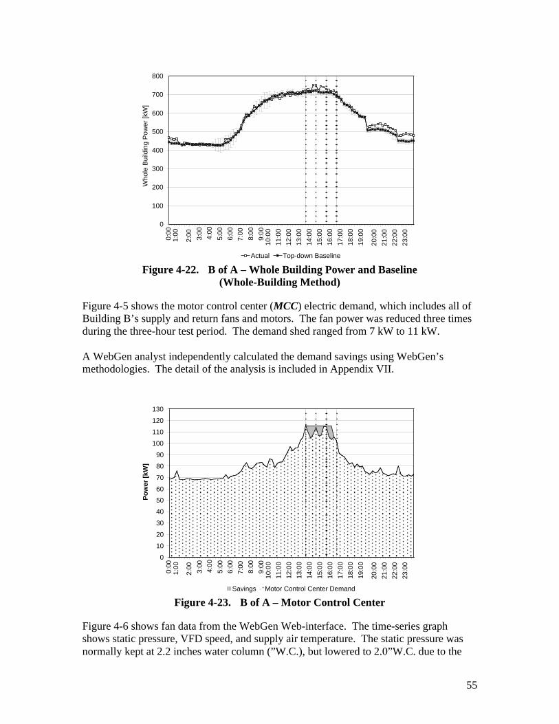
55
0
100
200
300
400
500
600
700
800
0:00
1:00
2:00 3:00
4:00
5:00
6:00
7:00
8:00
9:00
10:0
0
11:0
0
12:0
0
13:0
0
14:0
0
15:0
0
16:0
0
17:0
0
18:0
0
19:0
0
20:0
0
21:0
0
22:0
0
23:0
0
Who
le B
uild
ing
Pow
er [k
W]
Actual Top-down Baseline
Figure 4-22. B of A – Whole Building Power and Baseline(Whole-Building Method)
Figure 4-5 shows the motor control center (MCC) electric demand, which includes all ofBuilding B’s supply and return fans and motors. The fan power was reduced three timesduring the three-hour test period. The demand shed ranged from 7 kW to 11 kW.
A WebGen analyst independently calculated the demand savings using WebGen’smethodologies. The detail of the analysis is included in Appendix VII.
0
10
20
30
40
50
60
70
80
90
100
110
120
130
0:00
1:00
2:00 3:00
4:00
5:00
6:00
7:00
8:00
9:00
10:0
0
11:0
0
12:0
0
13:0
0
14:0
0
15:0
0
16:0
0
17:0
0
18:0
0
19:0
0
20:0
0
21:0
0
22:0
0
23:0
0
Po
wer
[kW
]
Savings Motor Control Center Demand
Figure 4-23. B of A – Motor Control Center
Figure 4-6 shows fan data from the WebGen Web-interface. The time-series graphshows static pressure, VFD speed, and supply air temperature. The static pressure wasnormally kept at 2.2 inches water column (”W.C.), but lowered to 2.0”W.C. due to the

56
static pressure reset strategy. The VFD speed was slightly reduced corresponding to thestatic pressure reset.
Static Pressure
Supply Air TemperatureVFD Speed %
Figure 4-24. B of A – WebGen Chart
GSA
Saving Verification MethodsGSA’s shed strategy implemented global zone temperature setpoint increase in coolingmode, and decrease in heating mode. The global setpoint temperature increase strategyaffects most of the HVAC system end-use equipment controls. The HVAC componentsconsidered as the controllable components for this saving analysis include the chillers,primary and secondary pumps, cooling towers, and fans.
One issue impacting the analysis of the demand shed is that GSA’s recently developedcooling strategy maximizes free cooling by cooling towers (tower free cooling). Becauseof this strategy, the chiller and the other related HVAC equipments operations provide anirregular load shape. Since this strategy has been implemented in some mornings beforeand during the 2-week test period, it is difficult to eliminate this irregular operationalpattern from baseline input data.
End-use Equipment Demand ExtrapolationAlthough many of the GSA electric submeter points for their HVAC equipment weretrended by the EMCS, some fan and pump submeter data necessary for the savinganalysis were not directly trended by the EMCS. These values had to be extrapolatedfrom other EMCS trend points. For constant volume systems, fan power was estimatedbased on equipment status and full load power from the mechanical specifications. For

57
variable volume systems, fan power was estimated from the VFD speed and scheduledpower10.
End-use Equipment Demand BaselineThe OAT regression model method was used to develop a baseline for each controllablecomponent for the saving analysis. Though internal loads mostly dominated the coolingloads in this building, we found that each component power has correlation against OAT.Individual baseline models were developed for the chillers, pumps, cooling towers, andfans respectively. This analysis is based on an assumption that the irregular patternscaused by the tower free cooling strategy would be averaged out by the model.
Saving ResultsFigure 4-7 shows GSA’s whole building power and the whole-building method baseline.Due to the tower free cooling operation in the morning, the chillers were off in the earlymorning, and turned on around 11:30 am. The whole building power peaked at 11:45 ambecause of the chiller startup. The global temperature setpoint increase (from 72 to 76°F) was implemented at 1:00 pm responding to the 15-minute ahead $0.30/kWh pricesignal. The whole building power dropped by 80 kW by 1:15 pm, and further dropped by75 kW at 1:30 pm. Using the whole-building method, the maximum demand saving was274 kW at 2:00 pm, which is 12% of whole building power. However, because thebaseline includes the intermittent impact of the tower free cooling strategy, the baselinecan have a wide error range.
0
500
1000
1500
2000
2500
3000
0:00
1:00
2:00 3:00
4:00
5:00
6:00
7:00
8:00
9:00
10:0
0
11:0
0
12:0
0
13:0
0
14:0
0
15:0
0
16:0
0
17:0
0
18:0
0
19:0
0
20:0
0
21:0
0
22:0
0
23:0
0
Who
le B
uild
ing
Pow
er [k
W]
Actual Whole-Building Method Baseline
Figure 4-25. GSA – Whole Building Power and Baseline (Whole-Building Method)
Figure 4-8 shows whole building power, HVAC demand and savings by the componentmethod. The OAT regression model was developed for each controllable component toestimate the savings. All of the component savings are summed. (See Appendix VII for
10 The equation used to calculate electric demand is: equipment demand [kW] = scheduled power [kW] x(VFD Speed [%])2. Some adjustment factors are also applied based on comparisons of the calculatedvalues to the submetered data.

58
the actual demand and OAT regression model graph of each controllable component).The maximum savings in whole building power by the component method was 240 kW(10%) at 3:45 pm.
0
200
400
600
800
1000
1200
1400
1600
1800
2000
2200
2400
2600
2800
0:00
1:00
2:00 3:00
4:00
5:00
6:00
7:00
8:00
9:00
10:0
0
11:0
0
12:0
0
13:0
0
14:0
0
15:0
0
16:0
0
17:0
0
18:0
0
19:0
0
20:0
0
21:0
0
22:0
0
23:0
0
Pow
er [k
W]
HVAC Others Savings (Component Method)
Figure 4-26. GSA – HVAC Demand and Savings (Component Method)
Figure 4-9 shows the electrical demand of each HVAC component. The fan powershowed the largest demand savings in the HVAC components. The fan controlsresponded quickly to the price signal setting. The fan demand dropped by 71 kW at 1:00pm and increased by 72 kW at 4:00 pm. The maximum demand saving of the fan powerwas 138 kW at 3:45 pm.
0
50
100
150
200
250
300
350
400
450
9:00
9:30
10:0
0
10:3
0
11:0
0
11:3
0
12:0
0
12:3
0
13:0
0
13:3
0
14:0
0
14:3
0
15:0
0
15:3
0
16:0
0
16:3
0
17:0
0
17:3
0
18:0
0
18:3
0
Po
wer
[kW
]
Chillers Cooling Tower Pumps Fans
Figure 4-27. GSA – HVAC Component Demand
When the first $0.30/kWh signal was received (1:00 pm), the setpoint increased from 72to 76 °F. Since the zone temperature setpoints were kept at 72 °F before the test started,

59
the zones were “pre-cooled” compared to the 76 °F setpoint. The chiller power wasreduced by approximately 40 kW until the zone temperatures rose to 76 °F. The chillerdemand crept up little by little, as some zones were reaching 76 °F. By 2:15 pm, thechiller demand increased, probably because many zones reached 76 °F and requiredcooling. Right after the chiller demand rise, the $0.75/kWh signal kicked in whichincreased the setpoint to 78 °F. The chiller demand dropped again. However, the zonetemperatures soon reached the new setpoint and chiller demand rose again. At 3:00 pm,the chiller demand further increased by the second $0.30/kWh signal which decreased thesetpoint back to 76 °F. However, the chiller demand suddenly decreased after 3:15 pm.This may have been caused by a factor irrelevant to the shed strategy. The chillerdemand increased again at 4:00 pm. when the setpoint decreased to 72 °F at the end ofthe test.
The pump electrical demand total contains the condenser water pumps, the primarychilled water pumps and the secondary chilled water pumps (See Appendix II for thepump demands on the test day). The pump demand increased to 167 kW at 2:45 pmresponding to staging-up of the chiller operation, and stayed at 130 kW until the end ofthe day’s scheduled operation. Because the pumps support the chiller operation, pumpdemand did not respond to the price signal promptly. The cooling tower demandfluctuated significantly during the test period, and remarkable demand saving could notbe determined.
Non-Energy IssuesZone temperatures for 39 zones (25 zones from 6 floors in North Tower, and 14 zonesfrom 3 floors in South Tower) were trended and analyzed at GSA. VAV damperpositions (19 zones) were also collected. Figure 4-10 shows the average of the 39 zonetemperatures during the test day, overlaid on the average zone temperature based on theprevious 18 days. (See Appendix VII for time-series charts of the zone temperatures andVAV damper positions for each floor). During normal building operation, the averagezone temperature was about 72 °F. During the shed, the average zone temperature roseby 1 °F (72 °F to 73 °F), although the shed strategy allowed the global temperaturesetpoint to increase to 76 °F at $0.30/kWh, and 78 °F at $0.75/kWh. The average zonetemperature dropped to below 72 °F after the shed ended.

60
68
69
70
71
72
73
74
0:00
1:00
2:00 3:00
4:00
5:00
6:00
7:00
8:00
9:00
10:0
0
11:0
0
12:0
0
13:0
0
14:0
0
15:0
0
16:0
0
17:0
0
18:0
0
19:0
0
20:0
0
21:0
0
22:0
0
23:0
0
Zon
e T
empe
ratu
re [D
egre
e F
]
Actual Previous Days Average
Figure 4-28. GSA – Zone Temperature
Individual zone temperature were also analyzed (see Appendix II). The controls for somezones responded to the global temperature setpoint strategy, with some zone temperaturesincreasing closer to or above 76 °F at the $0.30/kWh signal, and 78 °F at the $0.75/kWhsignal. However, most of the zone temperatures were not affected at all. Most VAVboxes (17 of 19 collected) didn’t change their damper positions during the test period.This may be because 1) the damper positions were less than 20% for most of VAV boxeswhich may be the minimum damper position allowed by the system in order to maintainminimum ventilation rates; and 2) the temperature difference might be within thecontrol’s deadband.
Although most of the monitored zones didn’t respond to the setpoint increase strategy,some zones indicated temperature changes and the HVAC component electric dataindicated demand savings due to the strategy. Since zone temperature and VAV damperposition data was collected for a small subset of the zones, it is hard to determine whathappened in the other zones.
Roche
Saving Verification MethodsThree Roche buildings, including A2 (office, auditorium), SS (office), and FS (cafeteria)participated in the Auto-DR test. Some of the fans in each building were turned off basedon the price signal. Since all the fans are constant volume, the fan electric demand wasextrapolated from the spot measurement data and normal operation schedule. Since thebuilding’s cooling loads are supplied from a cooling plant that serves multiple buildings,only the fan power is counted as a controllable load. We did not evaluate whether therewas any reduction in the cooling loads supplied to the buildings from the central plant.

61
Saving ResultsFigure 4-11 shows the whole building power and the whole-building method baselineapplied to all three buildings. The power measurements for each building and the whole-building baseline models are shown in Appendix VII. Building FS (cafeteria) electricdemand had several spikes in the morning because of food preparation. Building FSdemand declined rapidly after 1:00 pm because occupants left after lunchtime. BuildingSS changed its equipment operation on October 30th, and reduced approximately 50 kWof its demand. The whole-building method may project higher demand savings thanexpected, because the whole-building method baseline was affected by the demandprofile change of Building SS.
The whole-building analysis (including all the three buildings) indicates that Rocheachieved maximum 164 kW (28%) of demand savings from 2:45 pm to 3:00 pm. Thelevels of demand shed due to the different price signals can be clearly seen in the demandprofile. The whole building power dropped by 71 kW at 1:00 pm at the first $0.30/kWhsignal due to the implementation of the fan shed strategy. The demand dropped furtherby 57 kW at 2:00 pm at the $0.75/kWh signal.
0
100
200
300
400
500
600
700
800
0:00
1:00
2:00 3:00
4:00
5:00
6:00
7:00
8:00
9:00
10:0
0
11:0
0
12:0
0
13:0
0
14:0
0
15:0
0
16:0
0
17:0
0
18:0
0
19:0
0
20:0
0
21:0
0
22:0
0
23:0
0
Who
le B
uild
ing
Pow
er [k
W]
Actual Whole-Building Method Baseline
Figure 4-29. Roche – Combined Whole Building Power and Baseline(Whole-Building Method applied to all Three Buildings)
Figure 4-12 shows whole building power, fan power and savings by the componentmethod. The whole building power was reduced by 70 kW due to the air handlershedding at Building A2 activated at the $0.30/kWh signal. It was further reduced by 37kW by Building SS and FS fan shedding at the $0.75/kWh signal. The maximum shed ofall three buildings was 107 kW. This site collected 5-minute interval data for the fanstatus. The status data verified that all the selected air handlers followed the price signalwithin five minutes after receiving the new price signal (1:00 pm, 2:00 pm, 3:00 pm, and4:00 pm).
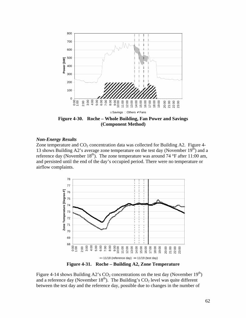
62
0
100
200
300
400
500
600
700
800
0:00
1:00
2:00 3:00
4:00
5:00
6:00
7:00
8:00
9:00
10:0
0
11:0
0
12:0
0
13:0
0
14:0
0
15:0
0
16:0
0
17:0
0
18:0
0
19:0
0
20:0
0
21:0
0
22:0
0
23:0
0
Po
wer
[kW
]
Savings Others Fans
Figure 4-30. Roche – Whole Building, Fan Power and Savings(Component Method)
Non-Energy ResultsZone temperature and CO2 concentration data was collected for Building A2. Figure 4-13 shows Building A2’s average zone temperature on the test day (November 19th) and areference day (November 18th). The zone temperature was around 74 °F after 11:00 am,and persisted until the end of the day’s occupied period. There were no temperature orairflow complaints.
68
69
70
71
72
73
74
75
76
77
78
0:00
1:00
2:00 3:00
4:00
5:00
6:00
7:00
8:00
9:00
10:0
0
11:0
0
12:0
0
13:0
0
14:0
0
15:0
0
16:0
0
17:0
0
18:0
0
19:0
0
20:0
0
21:0
0
22:0
0
23:0
0
Zo
ne
Tem
per
atu
re [
Deg
ree-
F]
11/18 (reference day) 11/19 (test day)
Figure 4-31. Roche – Building A2, Zone Temperature
Figure 4-14 shows Building A2’s CO2 concentrations on the test day (November 19th)and a reference day (November 18th). The Building’s CO2 level was quite differentbetween the test day and the reference day, possible due to changes in the number of

63
occupants. Based on the data available, it is difficult to correlate the CO2 changes duringthe shed period to the fan shed strategy. However, the CO2 concentration immediatelydecreased at the end of the test (4:00 pm). This was caused by turning back on the airhandlers, which were off during the DR test. During the test period, the CO2
concentration was lower than 500 ppm11, and there were no indoor air quality complaints.
360
380
400
420
440
460
480
500
520
540
560
0:00
1:00
2:00 3:00
4:00
5:00
6:00
7:00
8:00
9:00
10:0
0
11:0
0
12:0
0
13:0
0
14:0
0
15:0
0
16:0
0
17:0
0
18:0
0
19:0
0
20:0
0
21:0
0
22:0
0
23:0
0
CO
2 [p
pm
]
SF12 11/18 (reference) SF56 11/18 (reference)SF12 11/19 (test) SF56 11/19 (test)
Figure 4-32. Roche – Building A2, CO2 Concentration
UCSB
Saving Verification MethodsUCSB implemented the Auto-DR test at their Main Library, three inter-connectedbuildings (Library II, III and IV). Since the energy manager occasionally implementedsome energy saving strategies at the buildings, the days he manually implemented energysaving strategies are eliminated from the baseline input data. Those manually controlleddays are October 15th, 16th and 23rd. All the data used in the saving analysis werecollected by the EIS. Prior to the test period, only whole building power and coolingpower data were trended. For the component level evaluation, new data points wereadded to the EIS trend derived from the EMCS (See Table 3-7). Several zonetemperatures were added to the data trend to evaluate the zone conditions. The supplyfan and cooling power are considered as the controllable components.
Supply FansThe VFD percent limit shed strategies were applied to Library II Supply Fan #1 through#5 and Library III Supply Fan #2. According to the average previous-day profile, theLibrary II supply fan demands were flat during afternoon. Though the OAT regression
11 Comfort criteria, with respect to human bioeffluents (odor) are likely to be satisfied if the ventilationresults in indoor CO2 concentrations less than 700 ppm above the outdoor air concentration (ASHRAE 62-2001).

64
model method was tried for these fans, the actual fan load was higher than the maximumrange of standard error of the model. Assuming the afternoon fan load was flat, thebaseline demands for the Library II supply fans were estimated from the 15-minutedemand prior to the shed. The Library III Supply Fan #2 demand was not constant and itdidn’t respond to the shed strategy, so the OAT regression model was used to estimatethe Library III Supply Fan #2 demand.
Cooling PowerThough the Library has a central chiller plant, it is separated from the whole buildingpower meter because the chiller plant supplies chilled water to a campus chilled waterloop. The cooling energy [Btu/h] supplied to the Library is converted to electric demand[kW]12. Baseline cooling power was estimated by OAT regression model.
Saving ResultsFigure 4-15 shows the whole building power of the Library and the whole-buildingmethod baseline. Based on the whole-building method analysis, the Library achieved amaximum 109 kW (14%) demand savings at 2:15 pm and 2:45 pm, during the $0.75/kWhperiod. The whole building power dropped by 48 kW at 1:00 pm as a result of the supplyfan VFD shed strategy. The whole building power further dropped by 86 kW at 2:00 pmdue to the deeper shed of supply fan VFD, static pressure limit, and cooling valveshutdown. The whole building power spiked at 3:00 pm. This spike was caused by therelease of the cooling valve.
0
100
200
300
400
500
600
700
800
900
0:00
1:00
2:00 3:00
4:00
5:00
6:00
7:00
8:00
9:00
10:0
0
11:0
0
12:0
0
13:0
0
14:0
0
15:0
0
16:0
0
17:0
0
18:0
0
19:0
0
20:0
0
21:0
0
22:0
0
23:0
0
Who
le B
uild
ing
Pow
er [k
W]
Actual Whole-Building Method Baseline
Figure 4-33. UCSB – Whole Building Power and Baseline(Whole-Building Method)
Table 4-7 shows the breakdown of whole building power and estimated savings by thecomponent method. The maximum whole building power savings was 240 kW (10%) at
12 Library cooling power [kW] = central plant power [kW] x Library cooling energy use [Btu/h] / totalcooling energy produced [Btu/h]
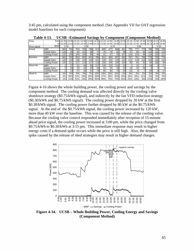
65
3:45 pm, calculated using the component method. (See Appendix VII for OAT regressionmodel baselines for each component)
Table 4-13. UCSB –Estimated Savings by Component (Component Method)Time from 12:45 13:00 13:15 13:30 13:45 14:00 14:15 14:30 14:45 15:00 15:15 15:30 15:45 16:00 16:15 16:30
to 13:00 13:15 13:30 13:45 14:00 14:15 14:30 14:45 15:00 15:15 15:30 15:45 16:00 16:15 16:30 16:45Price signal $/kW
Actual WBP 804 756 753 763 758 672 685 677 688 841 795 777 770 798 796 793Supply Fans 120 94 94 101 98 77 76 79 81 98 97 95 94 116 116 115Cooling Power 122 108 100 103 86 40 21 27 25 147 118 103 99 114 109 111
Baseline WBP 802 794 803 802 813 789 814 800 807 822 797 791 788 778 793 776Supply Fans 120 119 118 124 122 121 120 122 125 122 121 119 118 116 116 115Cooling Power 120 121 127 119 117 113 106 106 100 104 95 94 92 94 106 94
Shed kW WBP -2 37 51 40 55 117 129 123 119 -19 1 15 17 -19 -3 -17Supply Fans 0 24 24 24 24 44 44 44 44 24 24 24 25 0 0 0Cooling Power -2 13 27 16 31 73 85 80 75 -43 -23 -9 -7 -20 -3 -17
Shed % WBP 0% 5% 6% 5% 7% 15% 16% 15% 15% -2% 0% 2% 2% -2% 0% -2%Supply Fans 0% 20% 21% 19% 20% 36% 37% 36% 35% 20% 20% 20% 21% 0% 0% 0%Cooling Power -2% 11% 21% 13% 26% 65% 80% 75% 75% -42% -24% -10% -8% -21% -3% -18%
0.10 0.100.30 0.75 0.30
Figure 4-16 shows the whole building power, the cooling power and savings by thecomponent method. The cooling demand was affected directly by the cooling valveshutdown strategy ($0.75/kWh signal), and indirectly by the fan VFD reduction strategy($0.30/kWh and $0.75/kWh signal). The cooling power dropped by 20 kW at the first$0.30/kWh signal. The cooling power further dropped by 80 kW at the $0.75/kWhsignal. At the end of the $0.75/kWh signal, the cooling power increased by 120 kW,more than 40 kW over the baseline. This was caused by the release of the cooling valve.Because the cooling valve control responded immediately after reception of 15-minuteahead price signal, the cooling power increased at 3:00 pm, while the price changed from$0.75/kWh to $0.30/kWh at 3:15 pm. This immediate response may result in higherenergy costs if a demand spike occurs while the price is still high. Also, the demandspike caused by the release of shed strategies may result in higher demand charges.
0
100
200
300
400
500
600
700
800
900
0:00
1:00
2:00 3:00
4:00
5:00
6:00
7:00
8:00
9:00
10:0
0
11:0
0
12:0
0
13:0
0
14:0
0
15:0
0
16:0
0
17:0
0
18:0
0
19:0
0
20:0
0
21:0
0
22:0
0
23:0
0
Pow
er [k
W]
WBP Savings Cooling Power
negative savings
Figure 4-34. UCSB – Whole Building Power, Cooling Energy and Savings(Component Method)

66
Figure 4-17 shows the total fan power and baseline. The total fan demand dropped by 24kW at 1:00 pm upon the receipt of the $0.30/kWh signal which initiated the VFDpercentage limit strategy. The total fan demand achieved 43 kW saving during the$0.75/kWh period.
0
20
40
60
80
100
120
140
0:00
1:00
2:00
3:00 4:00
5:00
6:00
7:00 8:00
9:00
10:0
0
11:0
0
12:0
0
13:0
0
14:0
0
15:0
0
16:0
0
17:0
0
18:0
0
19:0
0
20:0
0
21:0
0
22:0
0
23:0
0
Pow
er [k
W]
Savings Supply Fan Total
Figure 4-35. UCSB – Fan Power and Savings
Non-Energy IssuesTwenty-one zone temperatures were trended at the Library. Figure 4-18 shows theLibrary’s average zone temperature on the test day and the reference day (average ofprevious 15 days). Zone temperatures of each building are given in Appendix VII.Although zone temperature increases were anticipated due to the shed strategy, averagezone temperature changes were within 1 °F during the test. The building’s has a largethermal mass, due to the building mass and books, so the zone temperature change mightbe moderated due to the thermal mass effect. There were no occupant complaints duringthe test.

67
67
68
69
70
71
72
73
0:00
1:00
2:00 3:00
4:00
5:00
6:00
7:00
8:00
9:00
10:0
0
11:0
0
12:0
0
13:0
0
14:0
0
15:0
0
16:0
0
17:0
0
18:0
0
19:0
0
20:0
0
21:0
0
22:0
0
23:0
0
Zon
e T
empe
ratu
re [D
egre
e F
]
Shed Day Average Zone Temp November Average Zone Temp
Figure 4-36. UCSB – Average Zone Temperature
Summary of Results
This section summarizes the results of the second test (November 19th). The demandsavings are presented as shed kW, shed %, and shed kW per square feet (kW/ft2). ShedkW is calculated by subtracting the actual whole building power from its baselinedemand. Shed percentage is defined as the percentage of savings in whole buildingpower. Shed kW/ft2 is the demand shed intensity, defined as the shed kW normalized bythe building conditioned floor area.
Table 4-7 shows the demand savings for each 15-minute period which were derived usingthe whole-building method. Table 4-8 shows the results summary for all sites by thecomponent method. The aggregated shed demand calculated using the componentmethod was similar to the results calculated using the whole-building method.
Based on the whole-building method, the maximum aggregated shed demand of all thefive sites was 519 kW. These savings were 11% of the whole building power and 0.30W/ft2. The maximum saving was achieved during the 2:15 pm to 2:30 pm interval,shortly after the $0.75/kWh price signal was received. Comparing the sites to each other,GSA achieved the largest shed kW (274 kW), Roche achieved the largest shed % (29%),and Albertsons achieved the largest shed kW/ft2 (0.75 kW/ft2) among the five sites.

68
Table 4-14. Summary of Estimated Savings of All Site (Whole-Building Method)Time from 12:45 13:00 13:15 13:30 13:45 14:00 14:15 14:30 14:45 15:00 15:15 15:30 15:45 16:00 16:15 16:30
to 13:00 13:15 13:30 13:45 14:00 14:15 14:30 14:45 15:00 15:15 15:30 15:45 16:00 16:15 16:30 16:45Price signal $/kW
Albertsons WBP kW 351 320 318 330 351 332 326 320 323 344 332 341 345 345 347 347Shed kW -1 24 25 25 12 22 18 27 37 10 10 8 13 5 0 1WBP shed % 0% 7% 7% 7% 3% 6% 5% 8% 10% 3% 3% 2% 4% 2% 0% 0%Shed W/spft -0.02 0.48 0.51 0.51 0.23 0.44 0.36 0.54 0.75 0.21 0.20 0.16 0.26 0.11 0.00 0.01
B of A WBP kW 720 726 729 717 752 751 723 746 742 731 726 718 721 706 682 664Shed kW -7 -15 -13 -2 -31 -28 -8 -33 -31 -17 -15 -6 -18 -13 6 10WBP shed % -1% -2% -2% 0% -4% -4% -1% -5% -4% -2% -2% -1% -3% -2% 1% 1%Shed W/spft -0.03 -0.07 -0.06 -0.01 -0.15 -0.13 -0.04 -0.16 -0.14 -0.08 -0.07 -0.03 -0.08 -0.06 0.03 0.05
GSA WBP kW 2248 2168 2093 2085 2091 2098 2086 2109 2178 2232 2184 2126 2085 2123 2178 2077Shed kW 141 195 264 271 274 257 259 219 195 141 217 246 223 176 48 83WBP shed % 6% 8% 11% 12% 12% 11% 11% 9% 8% 6% 9% 10% 10% 8% 2% 4%Shed W/spft 0.14 0.20 0.27 0.28 0.28 0.26 0.26 0.22 0.20 0.14 0.22 0.25 0.23 0.18 0.05 0.08
Roche WBP kW 658 587 569 558 555 498 458 425 412 465 463 457 450 522 527 454Shed kW 12 72 89 75 77 118 150 154 165 113 105 102 92 12 4 27WBP shed % 2% 11% 14% 12% 12% 19% 25% 27% 29% 20% 19% 18% 17% 2% 1% 6%Shed W/spft 0.06 0.38 0.47 0.39 0.40 0.61 0.78 0.80 0.86 0.59 0.55 0.53 0.48 0.06 0.02 0.14
UCSB WBP kW 804 756 753 763 758 672 685 677 688 841 795 777 770 798 796 793Shed kW -9 47 55 35 40 109 100 109 98 -70 -17 -3 -4 -32 -13 -27WBP shed % -1% 6% 7% 4% 5% 14% 13% 14% 12% -9% -2% 0% -1% -4% -2% -4%Shed W/spft -0.03 0.16 0.19 0.12 0.14 0.38 0.35 0.38 0.34 -0.24 -0.06 -0.01 -0.02 -0.11 -0.05 -0.09
Total WBP kW 4781 4557 4462 4452 4507 4351 4278 4276 4342 4612 4499 4418 4371 4494 4528 4334Shed kW 136 323 421 405 371 477 519 476 465 178 301 346 305 149 44 94WBP shed % 3% 7% 9% 8% 8% 10% 11% 10% 10% 4% 6% 7% 7% 3% 1% 2%Shed W/spft 0.08 0.19 0.24 0.24 0.22 0.28 0.30 0.28 0.27 0.10 0.17 0.20 0.18 0.09 0.03 0.05
0.10 0.100.300.750.30
WBP: whole building powerShed: demand saving (= baseline demand – actual demand)WBP shed %: demand saving ratio in whole building powerShed W/ft2: demand saving per square feet
Table 4-15. Summary of Estimated Savings of All Site (Component Method)Time from 12:45 13:00 13:15 13:30 13:45 14:00 14:15 14:30 14:45 15:00 15:15 15:30 15:45 16:00 16:15 16:30
to 13:00 13:15 13:30 13:45 14:00 14:15 14:30 14:45 15:00 15:15 15:30 15:45 16:00 16:15 16:30 16:45Price signal $/kW
Albertsons Shed kW 0 22 26 26 26 39 41 41 41 30 26 26 26 9 -1 -1WBP shed % 0% 6% 8% 7% 7% 10% 11% 11% 11% 8% 7% 7% 7% 3% 0% 0%Shed W/spft 0.00 0.44 0.52 0.52 0.52 0.78 0.82 0.83 0.83 0.60 0.52 0.52 0.52 0.18 -0.02 -0.01
B of A Shed kW 0 0 6 11 7 1 8 8 0 0 9 12 0 0 0 0WBP shed % 0% 0% 1% 1% 1% 0% 1% 1% 0% 0% 1% 2% 0% 0% 0% 0%Shed W/spft 0.00 0.00 0.03 0.05 0.03 0.00 0.04 0.04 0.00 0.00 0.04 0.06 0.00 0.00 0.00 0.00
GSA Shed kW 75 164 185 161 204 165 192 156 146 149 238 240 223 109 40 54WBP shed % 3% 7% 8% 7% 9% 7% 8% 7% 6% 6% 10% 10% 10% 5% 2% 3%Shed W/spft 0.08 0.17 0.19 0.16 0.21 0.17 0.20 0.16 0.15 0.15 0.24 0.25 0.23 0.11 0.04 0.05
Roche Shed kW 0 70 70 70 70 107 107 107 107 70 70 70 70 0 0 0WBP shed % 0% 11% 11% 11% 11% 18% 19% 20% 21% 13% 13% 13% 14% 0% 0% 0%Shed W/spft 0.00 0.37 0.37 0.37 0.37 0.56 0.56 0.56 0.56 0.37 0.37 0.37 0.37 0.00 0.00 0.00
UCSB Shed kW -2 37 51 40 55 117 129 123 119 -19 1 15 17 -19 -3 -17WBP shed % 0% 5% 6% 5% 7% 15% 16% 15% 15% -2% 0% 2% 2% -2% 0% -2%Shed W/spft -0.01 0.13 0.18 0.14 0.19 0.40 0.45 0.43 0.41 -0.07 0.01 0.05 0.06 -0.07 -0.01 -0.06
Total Shed kW 73 294 338 307 362 429 477 436 414 231 344 363 337 98 36 36WBP shed % 2% 6% 7% 6% 7% 9% 10% 9% 9% 5% 7% 8% 7% 2% 1% 1%Shed W/spft 0.04 0.17 0.20 0.18 0.21 0.25 0.28 0.25 0.24 0.13 0.20 0.21 0.20 0.06 0.02 0.02
0.100.10 0.30 0.75 0.30
Impact of Early Implementation and End of Shed Strategies
As a general trend, all sites except B of A responded approximately 15 minutes earlierthan when the price signal took effect (B of A’s demand shed was too small to identifythe result). For example, Albertsons reduced the demand a few minutes after 1:00 pmwhile the price signal rose at 1:15 pm. The system also responded 15 minutes earlierwhen the price signal fell. The price signal is designed to inform 15-minute ahead price

69
(for example, the signal received at 1:00 pm tells the future price of 1:15 pm). This wasin order to give the systems preparation time to change their operation before the pricechange. The result indicates these sites could respond to the signal and changed theoperation within a few minutes. The issue is that the shed strategies were disabled assoon as the system received the lower price signal, and therefore the demand increased 15minutes before the high price period ended. This may cause higher electricity chargesdespite of the demand response effort.
Demand Shed Related to Price Signal
Figure 4-19 and Figure 4-20 show shed kW and shed W/ft2 of each site averaged by each1-hour price signal level. The largest shed was at GSA, maintaining over 150 kW duringthe entire shed period. The greatest demand shed intensity was at Albertsons, with 0.4 to0.7 W/ft2 during the shed period. All but the B of A site shed at least 0.15 W/ft2.
0
50
100
150
200
250
Albertsons BofA GSA Roche UCSB
Ave
rag
e P
ow
er S
avin
g [
kW]
1st Hr.=$0.30/kWh 2nd Hr.=$0.75/kWh 3rd Hr.=$0.30/kWh
Figure 4-37. Average Shed kW by Price Signal Level (Component Method)
0.00
0.10
0.20
0.30
0.40
0.50
0.60
0.70
0.80
0.90
Albertsons BofA GSA Roche UCSB
Ave
rag
e P
ow
er S
avin
g In
ten
sity
[W
/ft2 ]
1st Hr.=$0.30/kWh 2nd Hr.=$0.75/kWh 3rd Hr.=$0.30/kWh
Figure 4-38. Average Shed W/ft2 by Price Signal Level (Component Method)

70
Whole Building Power and Aggregated Savings
Figure 4-21 shows the actual whole building power of all five sites and aggregateddemand savings, calculated by the component method. The total demand reductionbegan at 1:00 pm (15 minutes before $0.30/kWh period) and were further reduced at 2:00pm (15 minutes before $0.75/kWh). The systems returned to the same shed strategiesused at the previous $0.30/kWh level at 3:00 pm. The systems returned to normaloperation at 4:00 pm.
0
1000
2000
3000
4000
5000
6000
0:00
1:00
2:00 3:00
4:00
5:00
6:00
7:00
8:00
9:00
10:0
0
11:0
0
12:0
0
13:0
0
14:0
0
15:0
0
16:0
0
17:0
0
18:0
0
19:0
0
20:0
0
21:0
0
22:0
0
23:0
0
Who
le B
uild
ing
Pow
er [k
W]
Albertsons B of A GSA Roche UCSB Savings
$0.75
$0.30
$0.30
* Savings are calculated by the component method.Figure 4-39. Summary of All Sites
Demand saving by the whole-building method and the component method were similar,though the similarities vary by site. Figure 4-22 shows a comparison of the whole-building method and the component method calculated shed kW for each site. Roche’swhole-building method savings is higher than that calculated by the component method,because the whole-building baseline was affected by an operational change of onebuilding in the site. The overall results suggest that the weather normalized whole-building profiles provide reasonable estimates. Whole building data are much easier tocollect and are more readily available than end-use and component data. Previous workhas shown that methods that do not account for weather have significant bias for largecommercial buildings (KEMA-Xenergy, 2003). We did not compare the weather-normalized whole-building analysis method with the flat 10-day average baseline used inmany DR evaluations.
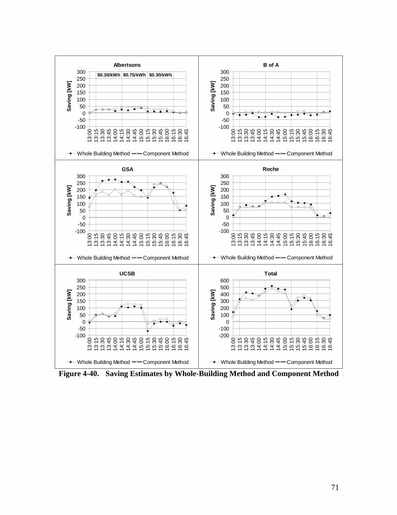
71
Albertsons
-100-50
050
100150200250300
13:0
013
:15
13:3
013
:45
14:0
014
:15
14:3
014
:45
15:0
015
:15
15:3
015
:45
16:0
016
:15
16:3
016
:45
Sav
ing
[kW
]
Whole Building Method Component Method
$0.30/kWh $0.75/kWh $0.30/kWh
B of A
-100-50
050
100150200250300
13:0
013
:15
13:3
013
:45
14:0
014
:15
14:3
014
:45
15:0
015
:15
15:3
015
:45
16:0
016
:15
16:3
016
:45
Sav
ing
[kW
]
Whole Building Method Component Method
GSA
-100-50
050
100150200250300
13:0
013
:15
13:3
013
:45
14:0
014
:15
14:3
014
:45
15:0
015
:15
15:3
015
:45
16:0
016
:15
16:3
016
:45
Sav
ing
[kW
]
Whole Building Method Component Method
Roche
-100-50
050
100150200250300
13:0
013
:15
13:3
013
:45
14:0
014
:15
14:3
014
:45
15:0
015
:15
15:3
015
:45
16:0
016
:15
16:3
016
:45
Sav
ing
[kW
]
Whole Building Method Component Method
UCSB
-100-50
050
100150200250300
13:0
013
:15
13:3
013
:45
14:0
014
:15
14:3
014
:45
15:0
015
:15
15:3
015
:45
16:0
016
:15
16:3
016
:45
Sav
ing
[kW
]
Whole Building Method Component Method
Total
-200-100
0100200300400500600
13:0
013
:15
13:3
013
:45
14:0
014
:15
14:3
014
:45
15:0
015
:15
15:3
015
:45
16:0
016
:15
16:3
016
:45
Sav
ing
[kW
]
Whole Building Method Component Method
Figure 4-40. Saving Estimates by Whole-Building Method and Component Method

72
5. Discussion: Organizational and Technological Issues
This section provides a discussion of the key lessons learned from this Auto-DR test.They have been organized into four main topic areas:
• Implementation and organizational challenges in deploying Auto-DR technology• Technical challenges at each site• Key lessons learned concerning unique attributes of the systems at each site that
further our understanding of the diversity of technology infrastructures amongthese facilities
• State-of-the-art technology and desirable features for future Auto-DR systems
5-1 Implementation and Organizational Challenges
There are a variety of implementation and organizational challenges that had to beaddressed during the execution of this project. After the research team defined the high-level objectives of the project, these objectives were conveyed to the key decision makersat each site as part of the recruitment effort. Facility and energy managers who were inthe position to understand and approve of a project of this magnitude tended to be spreadthin between important management responsibilities. As these managers delegatedproject responsibilities to their staffs, progress often stalled. The tasks necessary toimplement Auto-DR systems at each site cut across several areas of expertise andauthority. To implement Auto-DR systems as designed in the November 2003 test, mostsites required input from facility managers, HVAC experts, EMCS programmers, Webservices programmers and IT managers. Defining, designing, coordinating andimplementing the details of each site’s system often required substantial effort from thefacility staff and the research team.
Web services is a relatively new technology, and most of the development teams had notused it prior to the test. But because of the simplicity of this technology, lack ofexperience was not a major impediment to success for any of the Auto-DR testdevelopment teams. However, even though learning Web services is simple for mostprogrammers in the IT community, development of this technology requiresprogramming skills beyond the ability of most EMCS “programmers”. Within mostEMCS field organizations, it is uncommon for EMCS programmers to broaden theirskills to include IT level programming expertise.
Within each Auto-DR test team, an IT professional programmed the Web services clientand business logic, while an EMCS professional programmed or configured the shedlogic. While this approach ultimately produced successful results, the addedorganizational complexity made scoping, development, testing and project managementmore difficult than if all of the required software changes could be conducted by oneperson or organization.

73
5-2 Overview of Technical Challenges
There were a number of specific technical challenges in conducting this test. This sectiondescribes four key issues: software compatibility, time zones, IT and EMCS failures, andhardware issues.
Software CompatibilityPlatform independence is one of the key attributes of well-designed Web services.However, platform dependencies are not always easy to spot. In the Auto-DR test, therewere compatibility issues associated with the server software that was developed withinthe Microsoft “.Net ” environment and two of the clients that were developed in Java orDelphi environments. These problems were not caused by inherent platformincompatibilities per se, but by the indiscriminate use of a text format rather than anotherformat more commonly used to display data. The problems were resolved by modifyingthe Web services server to use a format that is more commonly used for data.
Time zonesThe developers, users, price server and polling clients were distributed across 3 timezones in continental North America. Thus, a common universal time zone was requiredfor use by all parties. Coordinated Universal Time (UTC) was selected as the standard.All parties used UTC in the lowest software levels, but most users preferred to see theirlocal time zone when interacting with the system on a HMI. In the test, programmersoften converted UTC to local time to improve the usability of time related data (e.g.,20:01 UTC was converted to 12:01 pm PST). But since this work was done withoutregard for users in other time zones, some time indication problems occurred with theviewing and logging at various sites. These problems were resolved by adopting a two-pronged approach; UTC was used for low level software and PST was used where timedata would be viewed or logged.
IT FailuresIn several cases, portions of the IT infrastructure failed for various reasons. AtAlbertsons, the polling client software stopped polling the price server inexplicitly justprior to the start of the test window. It was restored minutes later after systemadministrators were alerted by telephone. An upgrade of the UCSB EIS software severalweeks before the test left the gateway software out of synch. Since the remote controlfunctionality was not functional in time for the test, a remotely controlled IP Relay wasadded to provide the control interface to the EMCS. During the first test window, B ofA’s monitored building was not commanded into shed mode for unknown reasons.
EMCS FailuresIn the first test window, two sites failed to properly enter shed mode due to failures in theEMCSs. At GSA, an I/O controller locked up and failed to initiate a shed mode. AtUCSB, the first test was marred by some EMCS points being “fixed” in manual mode,unable to automatically respond to remote commands to enter certain shed strategies.

74
Hardware IssuesDuring the installation and early testing phase of the project, Albertsons managementreported that the chicken cooker lost power during the shed test of the freezer case lights.Further research of the electric trend logs showed an intermittent load profile that wasconsistent with that of an electric cooker on the same circuit as the freezer case lights.The cooker profile appeared several times per day starting several months prior.Albertsons management verified that the chicken cooker was installed earlier thatsummer on the date that the mysterious load profile was first observed. Rather thanperform costly revisions to high voltage wiring, the problem was resolved by modifyingthe EMCS software so as to remove the chicken cooker and freezer case lights from theshed strategy.
5-3 Lessons from each Site
This section identifies lessons learned based on the unique attributes of each participatingfacility. Issues related to the controls and communications infrastructures and shedstrategies are discussed for each system.
Albertsons System Overview
The Albertsons building telemetry data system is split between two systems. The EMCS(excluding electric monitoring) is accessed via dial-up modem. EIS data are available viaany Web browser through the Engage/eLution site. The lack of integrated systems makesenergy management and analysis more difficult for facilities staff.
Albertsons’ enterprise networks and control networks are tightly integrated. Albertsons’corporate WAN is used communicate between the business logic /polling client and theon-site IP I/O device. This enterprise network is also used for mission critical point ofsale data communications within the Albertsons organization. The fact that the energydata are shared and communicated over the mission critical enterprise network indicates ahigh level of trust and collaboration between Albertsons core business managers andAlbertsons energy managers.
Albertsons Shed Strategy Impacts
The shed strategy was not objectionable to the store managers or patrons. Although thetransition between 100% overhead lighting to 50% was noticeable, there were nocomplaints. The reduction of overhead light appeared to make the other light sources inthe store, such as case lights, seem more intense. There is no evidence that the freezerdoors fogged up during the shed, even though the anti-sweat heaters were switched tonight mode. If the transition of overhead lights to 50% were gradual (e.g., through use ofdimmable ballasts) the entire shed would probably not be noticeable.

75
Bank of America System Overview
The enterprise networks and control networks are tightly integrated. B of A’s corporateWAN is used to communicate across the country to the on-site gateway. This network isalso used for mission critical financial data communications within the B of Aorganization. Like Albertsons, the fact that the energy data are shared and communicatedover the mission critical enterprise network indicates a high level of trust andcollaboration between B of A’s core business managers and B of A’s energy managers.The use of highly secure and reliable hardware VPN routers and the use of a co-location(co-lo) to host the polling client and business logic computers are indications that systemavailability and security are high priorities to B of A.
When the WebGen system takes action to reduce energy at its connected sites, it uses acentralized control paradigm. While demand response systems are inherently centralized(signals to shed loads are generated in a one-to-many relationship), centralized control forday-to-day operation is less common.
In most control system markets (commercial buildings, industrial controls, etc.) there hasbeen a trend for several decades toward distributed or de-centralized control. Indistributed control architectures, the control logic is physically moved as close to thesensors and final control elements (relays, valves, etc.) as possible. Distributed controlsystems have traditionally been less costly, more flexible and more robust thancentralized systems. However, in the IT community there has been a movement towardhosted solutions, application service providers (ASPs) and other centralized solutions.Ubiquitous Internet connectivity and advances in IT equipment have made these systemsless costly, more flexible and more robust for certain applications.
The WebGen system alternates between centralized and decentralized paradigms oncycles of about twenty minutes. One minute a fan system maintains a setpoint entered byonsite building operators. In the next minute, a neural network algorithm defines thesetpoint from over 3000 miles away.
B of A Shed Strategy Impacts
With regard to the shed strategy employed at this site, there is no evidence that themodest reduction in duct static pressure for durations of twenty minutes caused anynegative comfort effects to the occupants during the test. However, as shown in themeasured data, the extent of the electric demand shed was also negligible.
If this strategy were expanded to produce significant electric sheds, this method may posesome fundamental drawbacks. In VAV systems, when duct static pressure is reducedbelow the minimum required by the terminal boxes, airflow is reduced in the zones. Butthe reduction is not shared evenly between all the boxes. The zones of greatest demandare the ones that are starved for air most immediately and most severely. In the B of Abuilding tested, the potential problem is exacerbated by the lack of sensors. Fan airflowis not measured and only nine “representative” zone temperature sensors are available for

76
the entire 211,000 ft2 building. There are not enough sensors to estimate the effects thatreductions in airflow would have on occupants.
GSA System Overview
The enterprise and EMCS infrastructures used to enable Auto-DR at this site are linkedtogether in a long series of serial components and communication links. The prototypesystem was assembled using spare parts at a low cost. With so many links, it is notsurprising that there was a communication failure due to an unexplained equipment lock-up during the first test. To make the system more robust, a review of the components andarchitecture should be conducted.
GSA Shed Strategy Impacts
The second test was quite successful as communications were functional from end-to-end. The shed strategy produced an electric shed about as large as the other four sitescombined. Because the temperature setpoint reset was at the zone level, comfort for eachoccupant could be maintained within the revised, relaxed constraints. To implement thisstrategy, it was necessary to revise the software parameters and some logic in each of the1,050 VAV terminal box controllers. For most EMCS systems, the labor required tomake these revisions would be substantial (one to three weeks). In this building, theprocess had been somewhat automated by previous system upgrades. This allowedEMCS reprogramming for Auto-DR to be conducted in about three hours.
Roche System Overview
The Tridium Niagra framework ties together the various EMCS protocols in a seamlessfashion. The Web interface provides operators compete monitoring and controlcapability from anywhere on the campus. It was relatively straightforward to interfacethe Auto-DR polling client and associated business logic to the system. The mostchallenging part of the project was setting up an “extra” computer outside of the Rochefirewall in the DMZ. This design allowed secure communications between the priceserver on the public Internet, the polling client on the DMZ computer and the Tridiumcomputer inside the corporate network.
UCSB System Overview
Remote monitoring and control of the EMCS and EIS data were available over theInternet prior to the Auto-DR test. However, at the time of the test, remote control of theEMCS was not available. The software gateway between the enterprise network and theEMCS network lost remote-control functionality during an “upgrade” of the SiliconEnergy server software. To meet the schedule of the Auto-DR test, in lieu of a gateway,an IP I/O controller was added to allow the Auto-DR business logic to initiate remote-control functions including shed initiation.

77
UCSB Shed Strategy ImpactsThe shed strategy proved to be very effective. The books and other mass in the Librarybuildings act as a thermal “flywheel” to help keep the space comfortable during the shedperiods. In addition, the sheds reduced airflow without shutting off fans completely. TheSanta Barbara’s coastal climate helped provide a temperate airflow even though thecooling valves were closed to save chiller energy.
5-4 State of the Art Auto-DR Systems
This section describes the attributes of state-of-art Auto-DR systems based ontechnologies that were either demonstrated or otherwise available at the time of theNovember 2003 Auto-DR test. A truly state-of-the-art Auto-DR system would use the“best of the best” components, systems and strategies from end to end. Such a systemwould be designed from scratch to meet a very specific set of requirements driven bybusiness cases or other factors. The “best” system would meet or exceed therequirements at the lowest installed cost.
Flexible Designs for the FutureToday’s state-of-the-art Auto-DR technology could be applied in many different ways,depending on the scenarios and use cases that they are designed to satisfy. As thescenarios, use cases, and driving forces behind Auto-DR become better defined, systemswill be designed and deployed accordingly. Since these design criteria are likely toremain in flux, Auto-DR system flexibility and future-proofing are a very high priorities.
FeaturesCustomers should have numerous options about how they can participate in Auto-DRprograms. For any given motivating force that drives customers to consider Auto-DR(e.g., price), each will have different circumstances under which they will want toparticipate. Customer flexibility must be built into any state-of-the-art Auto-DR system.They should have the ability to use custom business logic that is applicable to their ownoperations. Some may choose to allow remote real-time sheds, while others may wantsome advanced warning via pager or cell phone and the ability to opt out, if desired.Other important features in state-of-the-art Auto-DR systems are two-waycommunications, real-time monitoring, high security, and high system availability.
Leveraging Trends in TechnologyThe lower the installed cost of state-of-the-art Auto-DR systems, the sooner they will findtheir way into mainstream use. One of the most important ways to keep costs low is toleverage existing trends in technology. The use of existing IT technology in Auto-DRsystems wherever possible is an important way to keep costs low. The public Internetand private corporate LAN/WANs are ideal platforms for Auto-DR controls andcommunications due to their ubiquity, especially in large commercial buildings. Inaddition, the performance of IT equipment (e.g., routers, firewalls, etc.) continues toimprove and equipment prices continue to drop. Auto-DR systems based on standard ITplatforms will also tend to be more scalable and secure than special purpose systemsdeveloped specifically for Auto-DR.

78
Enterprise, EMCS and EIS IntegrationAnother way to obtain high system performance and keep the system costs low is throughincreased integration within the building. Since energy data from EISs are simplyanother type of measured data, EISs and EMCSs should share the same networks so as tomaximize system performance and functionality and minimize cost. In addition toeliminating a redundant EIS network, other aspects of the system are also unified throughthis approach. Use of an integrated EMCS/EIS database and associated archiving andvisualization tools increases user functionality while reducing cost. The ability to changesetpoints for HVAC equipment and observe and analyze the effect on electricity use fromthe same HMI is an important enhancement to both the EMCS and EIS.
State-of-the-art Auto-DR systems should have tight integration between the EMCS/EISnetwork and the enterprise networks within buildings. This strategy maximizes theperformance, distribution and availability of the building data, while minimizing theinstallation and maintenance costs. In systems in which EMCSs and EISs are highlyintegrated with enterprise networks and the Internet, managing the flow of information isgreatly simplified.
Once remote telemetry to EMCS and EIS is connected via enterprise networks, additionalfunctionalities are enabled. While the need for localized field maintenance remains,geographic limitations on the distribution of building information virtually disappear.Reliable, distributed information about the operation of EMCS/EISs can actually reducemaintenance costs. By remotely determining operating conditions, equipment run-time,and error codes, maintenance workers can be dispatched in a more efficient fashion. Inaddition, once the integrated enterprise EMCS/EIS infrastructure is in place, faultdetection and diagnostic (FDD) programs and other software tools can further reduceongoing operational costs. Other remote telemetry applications include energymanagement, energy forecasting, aggregation, access control and regulatory recordkeeping.
In a state-of-the-art Auto-DR system, remote telemetry to the EMCS/EIS should beprovided via password protected Web servers. Various levels of access should beprovided for different types of users. Maintenance workers and accountants may onlyneed monitoring access, while facility engineers may require complete control oversetpoints and programming logic.
The network architecture of today’s state-of-the-art Auto-DR system would tend to beflatter than that for most of the sites in the November 2003 test. A flat architecture is onein which there are a minimum number of layers of control network protocols between thefront-end HMI and final control and monitoring elements such as actuators and sensors.The most robust and least costly systems should have no more than one enterprisenetwork protocol and one control network protocol.
Open StandardsFor flexibility and future-proofing as well as the option to choose “best of breed”products, state-of-the-art Auto-DR systems should use open standards wherever possible.Unlike proprietary systems, truly open systems are interoperable. In other words, a

79
device from one company (e.g., Cisco) will easily and naturally reside on a network withproducts from other companies (e.g., Nortel). Most products in enterprise networks areinteroperable. They all communicate using the TCP/IP protocol and can be set up andmanaged using common network management tools.
TCP/IP is clearly the worldwide protocol of choice for LAN/WANs, the Internet andenterprise networks. There are several open standard control network protocols includingBACnet (ASHRAE Standard 135-2001) and LonTalk (ANSI/EIA/CEA 709.1). Althoughthe use of the meta-language XML is becoming a standard framework for communicatingover enterprise networks and the Internet, XML alone does not define data formats thatcan be used to convey measured building or energy data. Organizations such as oBIX,BACnet XML and OPC XML are developing standards of this type.
Shed StrategiesState-of-the-art shed strategies should be designed to minimize discomfort,inconvenience, and loss of revenue for the participating sites. Shed strategies should bedevised by customers to meet their needs. In general, shed strategies that use finegranularity closed-loop control are less likely to negatively impact building occupants fora given demand shed. Ideally, sheds would vary commensurately with a variable shedsignal. Transitions should be fast enough to be effective, but slow enough so thattransitions are not noticed by the building occupants.
In addition to HVAC control strategies, lighting and other switch-able loads should beconsidered for sheds as well. By increasing the Auto-DR controlled load to the pointwhere it approaches the whole building load, each load type (e.g., HVAC, lighting, etc.)would need to shed a smaller amount in order to achieve a given shed target for the wholebuilding.

80
6. Summary and Future Research Topics
General Findings and Research Issues
In general, this study has shown that Auto-DR is technically feasible, althoughconsiderable effort from the research team was needed to guide the development of thistechnology at several of the case study sites. This study has obtained detailedinformation concerning numerous topics regarding DR and Auto-DR. We have madeconsiderable progress in characterizing DR controls and communications systems forlarge facilities and in evaluating the specific DR shed strategies. We’ve also madeextensive progress in developing a preliminary conceptual design for a communicationsinfrastructure using XML and Web services. The technology presented here offers aglimpse of what may be possible for a large-scale deployment effort. We have also madeprogress in developing methods to measure and quantify the DR shed. The wholebuilding and component level analysis methods showed good agreement with each other,allowing for flexibility in the level of monitoring required to quantify the shed impacts.
It is important to outline key outstanding issues that should be addressed in futureresearch. One key question is how these strategies and technologies would perform inwarm weather that is more typical of DR events. There were no complaints recordedfrom these DR strategies. However, the buildings were not aggressively “pushed” toshed large amounts of power. Facility managers may require payment for largerinterventions and tests. A related issue is how both the communications and controltechnology infrastructure and the DR strategies can be used in today’s DR programs inCalifornia.
While the DR strategies used at each site were developed on a custom basis, there is aneed to gain more knowledge with how these strategies can be generalized. Thisknowledge will require market assessment of the capabilities of controls andcommunications systems, including remote connectivity and linkages between zones andcentral systems. As mentioned, there may be other strategies to help maximize DR andminimize the loss of services. A broader analysis of DR strategies is needed.
Perhaps the largest outstanding issue not addressed in this study is the costs and benefitsof bringing Auto-DR functionality to typical existing buildings and industrial facilities.Evaluating such costs will be highly dependent on a good characterization ofcommunications and control systems in today’s facilities. Further work on characterizingthe costs for the existing systems is needed to help understand the total costs and benefitsof such technology. The benefits include energy savings, and there is a need to keepenergy efficiency on the forefront of this area’s research efforts to ensure the technologyhas dual use and is used in a optimal manner. Assessing the benefits of DR or Auto-DRwill require a careful analysis of DR programs and developing scenarios that explore howlarge facilities might participate in these programs. These scenarios should consider real-time pricing, critical peak pricing, demand bidding, and other DR tariffs and programs.The economic perspectives can consider both the end-use customer and the societal costsand benefits of DR and Auto-DR.

81
Need for Technical Resources
As a technology-research oriented project, the research team developed new knowledgeabout DR that is not widely available. DR is a complex concept. Facility operators needto understand DR economics, controls, communications, energy measurement techniques,and the relation between changes in operation and electric demand. Such understandingmay involve numerous people at large facilities. Facility managers need good knowledgeof controls, and current levels of outsourcing of control services complicateunderstanding of control strategies and system capabilities.
Examples of information needed to facilitate DR in general include guides on DRstrategies and measurement and analysis tools and techniques to predict and measure DR.These tools should include building operational information and economic analysis tools.DR functional and commissioning tests are needed to guide facility managers through theprocess of identifying and testing DR strategies. Such techniques should ideally belinked to retro-commissioning guides that link energy savings and control optimization toDR.
One key finding of our research was that the controls and communications systems arecomplex. Limited information at each site was available to characterize the linkages andtechnology infrastructure. Facility managers need improved facility documentation asthe industry attempts to push today’s often broken control systems into advancedapplications like DR. If we achieve success in understanding how to specify and describethese controls and communications infrastructures, it may prove useful to require suchimproved documentation in building codes of the future. Similarly, future work shouldexplore requiring circuiting of non-critical end-uses and control strategies in newbuildings to facilitate DR in new buildings through the building code process.
Organizational Findings and Future Directions
Providing energy is a complex endeavor. Making sure that every customer has secure,reliable and safe power is a tremendous accomplishment of modern civilization. Theprovision of such power has relied on a paradigm that is changing. Today, good energyservices imply not merely providing safe, uninterruptible power, but supporting demandresponsiveness. The present energy industry does support these goals, although there isuniversal acknowledgement among the five Auto-DR participants that these programs arenecessary. These Lead Users cannot provide the leadership to develop DR technology ontheir own, although they are excellent partners for continuing research.
There are few industries and institutions that do not have Lead Users. In the case ofDemand Response, the Lead Users may not identify themselves. One reason for this isthat Demand Response programs are not mature in California. Facility managers valuesafety and security of information over demand responsiveness. It will be important forthe researchers to target clusters of lead users and educate them about the long termlikelihood of demand response programs and guide mid-level managers through theircumbersome bureaucracies towards participation in these programs.

82
Future related research will need to evaluate the costs and benefits of new demandresponse programs and tariffs in California. Such information should be provided to theexisting Lead Users to ensure that they become part of the extended demand responseresearch team. They should be encouraged to share some of the financial burden toparticipate in DR, but their costs should remain low until DR has been economicallyproven. They are unlikely to have continued interest in this work unless more lucrativeDemand Response programs develop. The lack of any mature Demand Responseprograms is an impediment to the research. Another impediment is that all five LeadUsers purchase energy from Direct Access suppliers.
Understanding and facilitating DR requires a long-term perspective, and technicalassistance will be needed for large commercial and industrial facilities. One promisingavenue to deliver technical services is to partner with knowledgeable vendors andcontrols suppliers. Facility managers and owners who fully understand their outsourcedtechnologies are rare, but an educated vendor can provide information and facilitatechange more easily. Further, an educated vendor can supply the essential information oncosts that the midlevel managers require.
Technology Issues
There are several key issues about future Auto-DR technology.
Scalability - While the Auto-DR infrastructure and associated components performedexceptionally in this test, additional technical issues associated with a full-scale Auto-DRdeployment are expected to be significant. Additional research is required to addressissues associated with deploying a real system in thousands or tens of thousands of sites.Scalable designs must consider installation and configuration methods, networkmanagement, version control and other long-term maintenance issues that have not beenconsidered in the scope of this test.
Security – What are the worst-case scenarios that could occur if an Auto-DR systemwere breeched by hackers? What security design and process measures should beconsidered in a deployable Auto-DR system?
Use Cases - What are the likely use cases for which a deployable Auto-DR systemshould be designed? A system designed primarily for emergency load relief may besubstantially different then a system designed to minimize operational costs on anongoing basis. What are the shed timing requirements of various use cases and what arethe timing characteristics of various Auto-DR systems and strategies?
Candidate Sites - What are the characteristics of a facility that make it a good candidatefor Auto-DR? What are the characteristics of facility management and engineering teamsthat will help assure that their sites would succeed in Auto-DR programs? What are themost practical ways to add Auto-DR to existing commercial buildings that lack existingremote telemetry to HVAC systems?

83
Intelligent Centralized Orchestration - If thousands of Auto-DR sites across the statewere “on-line” how should they be orchestrated? From a centralized operations center,what criteria would determine which sites or groups of sites should be commanded toshed? To what degree could centralized automation act as a “traffic cop” to help thecapacity meet the demand in each region? Is it possible to create flexible groupingscustomized to meet the needs of any given shed event? What would be thecharacteristics of such a system?
Technology Trends - As building systems including EMCS, EIS, security, fire andtelephones are all moving toward inclusion into an enlarged more integrated definition ofthe “enterprise network”, the technologies used in the enterprise are shifting as well.How will these trends affect the future of Auto-DR? How will wireless devices be usedin Auto-DR? How will the eventual implantation of the next Internet protocol, IPv6affect Auto-DR?

84
7. References
California Energy Commission. 2003. “2003 Integrated Energy Policy Report. Docket#02-IEP-01”. Adopted by the Commission November 12, 2003. California EnergyCommission publication number 100-03-019F.
Flynn, P. ( Editor). 2003. “The XML FAQ.” Maintained on behalf of the World WideWeb Consortium's XML Special Interest Group, version 3.01 (publication number 2003-01-14).
Goldman, C.A., M. Kintner-Meyer, and G. Heffner. 2002. “Do “Enabling Technologies”Affect Customer Performance in Price-Responsive Load Programs?” Lawrence BerkeleyNational Laboratory, Berkeley, CA. LBNL-50328.
Goldman, C.A., N. Hopper, O. Sezgen, M. Moezzi, R. Bharvirkar, B. Neenan, R.Boisvert, P. Cappers, and D. Pratt. 2004. “Customer Response to Day-ahead WholesaleMarket Electricity Prices: Case Study of RTP Program Experience in New York.”Prepared for The California Energy Commission. LBNL Report (Forthcoming).
International Performance and Measurement Verification protocol (IPMVP). 2001.“IPMVP Volume I: Concepts and Options for Determining Energy and Water Savings.”
KEMA-Xenergy. 2002. “Enhanced Automation: Technical Options Guidebook.”California Energy Commission publication number 400-02-005F.
KEMA-Xenergy. 2003. “Protocol Development for Demand Response Calculation -Findings and Recommendations: Consultant Report”. California Energy Commissionpublication number 400-02-017F.
Kinney, S., M.A. Piette, L. Gu, and P. Haves. 2001. “Demand Relief and WeatherSensitivity in Large California Commercial Office Buildings.” Proceedings of the 2001International Conference for Enhanced Building Operations. LBNL-48285.
Kintner-Meyer, M., C. Goldman, O. Sezgen, and D. Pratt. 2003. “Dividends withDemand Response.” ASHRAE Journal, October.
Koomey, J., and R. Brown. 2002. “The Role of Building Technologies in Reducing andControlling Peak Electricity Demand.” LBNL-49947. September.
Motegi, N., M.A. Piette, S. Kinney, and K. Herter. 2003a. “Web-based EnergyInformation Systems for Energy Management and Demand Response in CommercialBuildings.” LBNL Report 52510.
Motegi, N., and M.A. Piette, S. Kinney, and Jim Dewey. 2003b. “Case Studies of EnergyInformation Systems and Related Technology: Operational Practices, Costs, and

85
Benefits.” Proceedings of the International Conference of Enhanced Building Operations.LBNL Report 53406.
Neenan, B., D. Pratt, P. Cappers, J. Doane, J. Anderson, R. Boisvert, Goldman, C., O.Sezgen, G. Barbose, R. Bharvirkar, M. Kinter-Meyer, S. Shankle and D. Bates. 2003.“How and Why Customers Respond to Electricity Price Variability: A Study of NYISOand NYSERDA 2002 PRL Program Performance.” LBNL-52209.
Nexant. 2002. “AB 29X and SB 5X Program Evaluation. First Quarter Report (January1 to March 1, 2002).” Submitted to the California Energy Commission. Contract #400-00-070.
Nexant. 2001. “AB 979, AB 29X and SB 5X Peak Load Reduction Programs.December 2001 Annual Report.” Submitted to the California Energy Commission andthe California State Legislature.
Piette, M.A, S. Kinney, LBNL; M. Levi, D. McBride and S. May. 2002. “GEMnet Statusand Accomplishments: GSA's Energy and Maintenance Network.” Proceedings of the2002 ACEEE Summer Study Proceedings. May 2002, LBNL-50733.
Piette, M.A., 1991. Controls to Reduce Electrical Peak Demands in CommercialBuildings. Center for the Analysis and Dissemination of Demonstrated EnergyTechnologies. CADDET Analyses Series 7, ISBN 90-72647-17-3. August 1991.
Shockman, C., O. Sezgen, N. Motegi, M.A. Piette, and D. Watson. 2004. “MarketTransformation Lessons Learned from an Automated Demand Response Test inCalifornia.” ACEEE Summer Study on Energy Efficiency in Buildings proceedings.August 2004.
Urban, G. L., and E von Hippel. 1988. "Lead User Analyses for the Development of NewIndustrial Products." Management Science volume 34, number 5 (May):569-82.
Webopedia. 2004. http://www.webopedia.com/TERM/X/XML.html. Accessed March15, 2004.

Development and Evaluation of Fully Automated Demand Response In Large Facilities
APPENDICES
March 30, 2004
Mary Ann Piette Osman Sezgen
David S. Watson Naoya Motegi
Lawrence Berkeley National Laboratory
Christine Shockman Shockman Consulting
Laurie ten Hope
Program Manager, Energy Systems Integration
Sponsored by the California Energy Commission


Table of Contents
Appendix I. Acronyms and Terminology............................................................ I-1 Appendix II. Methodology – Additional Details..................................................II-1 Appendix II-1. Whole-Building Level Method, Additional Detail............................ II-1 Appendix III. Sample Memorandum of Understanding .................................... III-1 Appendix III-1. Project Participant Memorandum of Understanding ........................III-1 Appendix III-2. Automated Demand Response Test Questionnaire ..........................III-4 Appendix III-3. Time Schedule for Demand Response Test Participants ..................III-6 Appendix III-4. Price Signal for the Automated Demand Responses Tests ...............III-7 Appendix III-5. RT Pricing Web Methods and XML Schema.................................III-10 Appendix IV. Participants List ........................................................................... IV-1 Appendix V. Site Questionnaires (Test 1, Test 2)................................................V-1 Appendix V-1. Site Questionnaires – Albertsons......................................................V-1 Appendix V-2. Site Questionnaires – Bank of America............................................V-3 Appendix V-3. Site Questionnaires – GSA Oakland.................................................V-5 Appendix V-4. Site Questionnaires – Roche.............................................................V-8 Appendix V-5. Site Questionnaires – UCSB ............................................................V-9 Appendix VI. Site Data Collection Points List ................................................... VI-1 Appendix VI-1. Albertsons – Point List................................................................... VI-1 Appendix VI-2. Bank of America – Point List......................................................... VI-1 Appendix VI-3. GSA Oakland – Point List.............................................................. VI-3 Appendix VI-4. Roche – Point List and Fan Spot Measurement Plan....................... VI-5 Appendix VI-5. UCSB – Shed Strategies and Point List .......................................... VI-9 Appendix VII. Additional Result Tables and Figures ........................................VII-1 Appendix VII-1. First Day Test Results ................................................................... VII-1 Appendix VII-2. B of A – Result Analysis by WebGen ........................................... VII-5 Appendix VII-3. GSA – Additional Figures............................................................. VII-7 Appendix VII-4. Roche – Additional Figures......................................................... VII-17 Appendix VII-5. UCSB – Additional Figures ........................................................ VII-19 Appendix VIII. Previous DR Participation and Site Contact ............................ VIII-1 Appendix VIII-1. Prior Demand Response Program Participation ............................VIII-1 Appendix VIII-2. Interaction with Site Contacts ......................................................VIII-4 Appendix VIII-3. Problems Encountered During Test Period...................................VIII-8


I-1
Appendix I. Acronyms and Terminology
Abstraction. In this document, the term “abstraction” is used with regard to translations between different communication protocols or I/O point mappings. In abstraction, details of one protocol or data format are added or removed in order to function properly in the other. Through translation and abstraction, low level protocols (such as EMCS protocols) can be changed into a common protocol or language (such as TCP/IP and XML). This process is often bi-directional (See translation, protocol, I/O, point mapping, EMCS, TCP/IP and XML). Auto-DR. Automated Demand Response BACnet. An open data communication protocol for building automation and control networks. A data communication protocol is a set of rules governing the exchange of data over a computer network. The rules take the form of a written specification (in BACnet's case they are also on compact disk) that spells out what is required to conform to the protocol. BACnet was developed under the auspices of ASHRAE. The BACnet standard is also an ANSI standard (http://www.bacnet.org/FAQ/HPAC-3-97.html, BACnet.org 2004). BACnet MSTP. Short for BACnet Master/Slave Twisted Pair. BACnet MSTP describes the characteristics of the BACnet communication protocol when used in a Master/Slave architecture over twisted pair wiring. Bandwidth. The amount of data that can be transmitted in a fixed amount of time. For digital devices, the bandwidth is usually expressed in bits per second (bps) or bytes per second. For analog devices, the bandwidth is expressed in cycles per second, or Hertz (Hz) (Webopedia, 2004). Business Logic. In the Auto-DR tests, business logic determines the EMCS actions to be implemented based on price and business rules. Client (computer). The client part of a client-server architecture. Typically, a client is an application that runs on a personal computer or workstation and relies on a server to perform the operations requested by the client. For example, an e-mail client is an application that enables you to send and receive e-mail. In the Auto-DR tests the clients at each site polled the server to get current pricing information. Co-lo. See Co-Location. Co-Location. A server, usually a Web server, that is located at a dedicated facility designed with resources which include a secured cage or cabinet, regulated power, HVAC sufficient to cool all the electronic equipment, dedicated Internet connection, security and support. These co-location facilities offer their customers a secure place to physically house their hardware and equipment as opposed to locating it in their offices or warehouse where the potential for fire, theft or vandalism is much greater. Most co-

I-2
location facilities offer high-security, including cameras, fire detection and extinguishing devices, multiple connection feeds, filtered power, backup power generators and other features to ensure a level of high-availability which is mandatory for all Web-based, virtual businesses. Co-location sites are being built at various points around the world to provide services to the rapidly expanding Web hosting and e-commerce marketplace. The term co-location is also known as co-lo (Webopedia, 2004). Control network. A network of controllers, data gathering panels and other devices that measure values from sensors and send commands to actuators. Control networks have been designed and optimized for the requirements of these systems including low installed cost and small communication packet sizes. Historically, many control networks have been based on RS-485 communications using proprietary protocols. Increasingly open protocols are being used including BACnet and LonTalk over RS-485 and Internet Protocols (IP). Control networks are generally separate from enterprise networks. Data logging. The process by which data from I/O points are logged into a database. Dewpoint. The temperature at which water vapor is saturated. Digital outputs (DO). In an I/O controller, digital outputs are used to command equipment on or off. Physically, a digital output consists of an automatically controlled relay contact. Constant volume fans and pumps and lights can be commanded on or off with a digital output (see I/O controller). DMZ. Short for demilitarized zone, a computer or small subnetwork that sits between a trusted internal network, such as a corporate private LAN, and an untrusted external network, such as the public Internet. Typically, the DMZ contains devices accessible to Internet traffic, such as Web servers. The term comes from military use, meaning a buffer area between two enemies (Webopedia, 2004). DR. Demand Response. EIS. Energy Information System. Embedded devices. Special purpose computers with the following attributes:
1) Targeted functionality with little, if any, flexibility for the user to add different programs or customize the device.
2) User interfaces are usually limited to allow targeted functionality only. May include small LCD screens, LEDs, buttons switches and knobs. QWERTY keyboards and Cathode Ray Tube display screens are generally not included.
3) Memory is usually cost optimized for the targeted functionality. Read only memory (ROM) and flash memory chips are usually used in lieu drives with spinning disks.

I-3
4) Form factor is specially designed for the targeted functionality. Examples of embedded devices include Internet routers, automotive engine computers and cell phones.
5) Often designed for reliable continuous operation with little or no human interaction.
EMCS. Energy Management and Control System. Enterprise. A business organization. In the computer industry, the term is often used to describe any large organization that utilizes computers. An intranet is an example of an enterprise computing system (Webopedia, 2004). Ethernet. A local-area network (LAN) architecture developed by Xerox Corporation in cooperation with DEC and Intel in 1976. Ethernet uses a bus or star topology and supports data transfer rates of 10 Mbps. The Ethernet specification served as the basis for the IEEE 802.3 standard, which specifies the physical and lower software layers. Ethernet uses the CSMA/CD access method to handle simultaneous demands. It is one of the most widely implemented LAN standards. A newer version of Ethernet, called 100Base-T (or Fast Ethernet), supports data transfer rates of 100 Mbps. The newest version, Gigabit Ethernet supports data rates of 1 gigabit (1,000 megabits) per second (Webopedia, 2004) Firewall. A system designed to prevent unauthorized access to or from a private network. Firewalls can be implemented in either or both hardware and software. Firewalls are frequently used to prevent unauthorized Internet users from accessing private networks connected to the Internet, especially intranets. All messages entering or leaving the intranet pass through the firewall, which examines each message and blocks those that do not meet the specified security criteria. There are several types of firewall techniques:
1) Packet filter: Looks at each packet entering or leaving the network and accepts or rejects it based on user-defined rules. Packet filtering is fairly effective and transparent to users, but it is difficult to configure. In addition, it is susceptible to IP spoofing.
2) Application gateway: Applies security mechanisms to specific applications, such as FTP and Telnet servers. This is very effective, but can impose performance degradations.
3) Circuit-level gateway: Applies security mechanisms when a TCP or UDP connection is established. Once the connection has been made, packets can flow between the hosts without further checking.
4) Proxy server: Intercepts all messages entering and leaving the network. The proxy server effectively hides the true network addresses.
In practice, many firewalls use two or more of these techniques in concert. A firewall is considered a first line of defense in protecting private information. For greater security, data can be encrypted (Webopedia, 2004).

I-4
Fully-Automated Demand Response. Fully-Automated Demand Response is initiated at a building or facility through receipt of an external communications signal – facility staff set up a pre-programmed load shedding strategy which is automatically initiated by the system without the need for human intervention. Gateway. Gateways used in building telemetry systems provide several functions. First, they connect two otherwise incompatible networks (i.e., networks with different protocols) and allow communications between them. Second, they provide translation and usually abstraction of messages passed between two networks. Third, they often provide other features such as data logging, and control and monitoring of I/O points. Generation. In electronics, computer equipment and software, the term “generation” is used to describe a major upgrade for which previous versions may or may not be compatible. High Availability. Used to quantify the “uptime” for computer servers and systems. High availability is a requirement for operation of mission critical systems. High availability systems are often described in terms of the number of “nines” of availability (i.e., four 9s or 99.99% means less than one hour of unscheduled downtime per year). HTTP. Short for HyperText Transfer Protocol, the underlying protocol used by the World Wide Web. HTTP defines how messages are formatted and transmitted, and what actions Web servers and browsers should take in response to various commands. For example, when you enter a URL in your browser, this actually sends an HTTP command to the Web server directing it to fetch and transmit the requested Web page (Webopedia, 2004). Human Machine Interface (HMI). Nowadays humans interact more with computer-based technology than with hammers and drills. Unlike tools, the visible shape and controls of a computer do not communicate its purpose. The task of an HMI is to make the function of a technology self-evident. Much like a well-designed hammer fits the user's hand and makes a physical task easy; a well-designed HMI must fit the user's mental map of the task he or she wishes to carry out (International Engineering Consortium (www.iec.org), 2004). In control systems, the HMI usually takes the form of a computer display screen with specially designed graphical representations of the mechanical systems or processes including real-time data from sensors. HVAC. Heating, Ventilation, and Air Conditioning. I/O. Abbreviation for Input/Output. Commonly used in the controls industry. Refers to inputs (such as sensors) and outputs (such as actuators) (see abstraction, point mapping and translation). I/O controller. A device that measures input values from sensors and commands outputs such as temperature control valves, usually to maintain a defined setpoint. An I/O controller has the internal intelligence to perform local control.

I-5
I/O module. A device that measures input values from sensors and commands outputs such as temperature control valves based on instructions from a remote controller. An I/O module usually does not have the internal intelligence to perform local control. Internet. A global network connecting millions of computers. More than 100 countries are linked into exchanges of data, news and opinions. Unlike online services, which are centrally controlled, the Internet is decentralized by design. Each Internet computer, called a host, is independent. Its operators can choose which Internet services to use and which local services to make available to the global Internet community. Remarkably, this anarchy by design works exceedingly well. There are a variety of ways to access the Internet, including through online services, such as America Online, and commercial Internet Service Providers (ISP) (Webopedia, 2004). References to the public Internet, as described here, are spelled “Internet” (capital “I”). The lesser used term, “internet” (lower case “i”), refers to a network of intranets that are usually privately operated (see intranet). Intranet. A network based on TCP/IP protocols (an internet) belonging to an organization, usually a corporation, accessible only by the organization's members, employees, or others with authorization. An intranet's Web sites look and act just like any other Web sites, but the firewall surrounding an intranet fends off unauthorized access. Like the Internet itself, intranets are used to share information (Webopedia, 2004). IP I/O device. A device that measures inputs (e.g., electric meter data) and controls outputs (e.g., relays) that can be measured and actuated remotely over a LAN, WAN or Internet using Internet Protocols (IP). IP relay. A device with a relay or relays that can be actuated remotely over a LAN, WAN or Internet using Internet Protocols (IP). ISO. Independent System Operator. IT. Short for Information Technology, and pronounced as separate letters, the broad subject concerned with all aspects of managing and processing information, especially within a large organization or company. Because computers are central to information management, computer departments within companies and universities are often called IT departments. Some companies refer to this department as IS (Information Services) or MIS (Management Information Services) (Webopedia, 2004). LAN. A computer network that spans a relatively small area. Most LANs are confined to a single building or group of buildings. Most LANs connect workstations and personal computers. Each node (individual computer) in a LAN has its own central processing unit (CPU) with which it executes programs, but it also is able to access data and devices anywhere on the LAN. This means that many users can share devices, such as laser printers, as well as data. Users can also use the LAN to communicate with each other

I-6
such as by sending e-mail. There are many different types of LANs with Ethernets being the most common for PCs (Webopedia, 2004). Load balancing. Distributing processing and communications activity evenly across a computer network so that no single device is overwhelmed. Load balancing is especially important for networks where it's difficult to predict the number of requests that will be issued to a server. Busy Web sites typically employ two or more Web servers in a load balancing scheme. If one server starts to get swamped, requests are forwarded to another server with more capacity. Load balancing can also refer to the communications channels themselves (Webopedia, 2004).
LonTalk™. An open communications protocol used in building control systems and other industries. Publicly published under ANSI/ EIA -709.1 - (American National Standards Institute/Electronic Industries Alliance). Since 1999, LonTalk protocol may be implemented on any microprocessor.
LonWorks™. Control and communication products available from Echelon Corporation and other companies using Echelon products. LonWorks products use LonTalk open protocol for communications (see LonTalk).
Machine-to-Machine (M2M). Machine to Machine (M2M) is a term used to describe the technologies that enable computers, embedded processors, smart sensors, actuators and mobile devices to communicate with one another, take measurements and make decisions - often without human intervention. Manual Demand Response. Manual demand response involves manually turning off lights or equipment; this can be a labor-intensive approach. MCC. Motor Control Center. Modbus. An open standard control network protocol originally developed by Modicon, a simple master/slave protocol over RS-485. Current protocol also supports TCP/IP over an Ethernet. Modbus is a common interface with electrical equipment such as meters and generators. It is not typically used for whole building EMCSs. Modem. A hardware device that allows computers to communicate with one another over any phone-based network. NOC. Short for network operations center, the physical space from which a typically large telecommunications network is managed, monitored and supervised. The NOC coordinates network troubles; provides problem management and router configuration services; manages network changes; allocates and manages domain names and IP addresses; monitors routers, switches, hubs and UPS systems that keep the network operating smoothly; and manages the distribution and updating of software and coordinates with affiliated networks. NOCs also provide network accessibility to users

I-7
connecting to the network from outside of the physical office space or campus (Webopedia, 2004). OAT. Outside air temperature. oBIX. Open Building Information eXchange is an industry-wide initiative to define open XML- and Web services-based mechanisms for building control systems. ODBC. Short for Open DataBase Connectivity, a standard database access method developed by Microsoft Corporation. The goal of ODBC is to make it possible to access any data from any application, regardless of which database management system (DBMS) is handling the data. ODBC manages this by inserting a middle layer, called a database driver, between an application and the DBMS. The purpose of this layer is to translate the application's data queries into commands that the DBMS understands. For this to work, both the application and the DBMS must be ODBC-compliant -- that is, the application must be capable of issuing ODBC commands and the DBMS must be capable of responding to them. Since version 2.0, the standard supports SAG SQL (Webopedia, 2004). Onboard. Refers to electronic components that are mounted on the main printed circuit board as opposed to components that are mounted remotely and connected via wires. Open protocol. A communications protocol that is used to communicate between devices of any compliant manufacturer or organization. Open protocols are published in a public forum for use by all interested parties (see proprietary protocol). Point mapping. The process by which I/O points are mapped to another system or protocol (see abstraction, I/O and translation). Point of sale (POS). Refers to all components in the POS system including bar code scanners, cash registers, printers and all communications equipment that is used to transfer information about the sale of each item back to a central database. At some sites in the Auto-DR tests, the point of sale communications infrastructure was used to command the shed of electric loads based on electricity pricing information. Poll. A method by which one computer requests information from another. Polling Client. In the Auto-DR tests, the polling client is the software used to poll the server to get the price signal. Price Server. In the Auto-DR tests, the price server is the common source for the current price information. Proprietary protocol. A communications protocol that is used to communicate between devices of one manufacturer or organization while effectively disallowing all other

I-8
devices to exist on the same network. Proprietary protocols are not published in a public forum (see open protocol). Protocol (data communication). A data communication protocol is a set of rules governing the exchange of data over a computer network. Public Switched Telephone Network (PSTN). International telephone system based on copper wires carrying analog voice data. This is in contrast to newer telephone networks based on digital technologies (Webopedia 2004). Pull architecture. In a client-server architecture, the client “pulls” information from the server by polling (see poll). Pulse. Contact closures that are measured by an I/O device. Pulses are often produced by electric meters and other devices to indicate a given unit of measurement (for example, 1 pulse = 1 kWh). Real-time. In real-time control and monitoring systems, data is measured, displayed and controlled at a rate fast enough that the system latencies are negligible compared with the process at hand. Acceptable latency can vary substantially based on the type of process (for example, from 1 millisecond to several minutes). Semi-Automated Response. Semi-Automated Response involves the use of building energy management control systems for load shedding, where a pre-programmed load shedding strategy is initiated by facilities staff. Sensor. a device that responds to a physical stimulus (heat, light, sound, pressure, magnetism, or a particular motion) and transmits a resulting impulse that can be used for measurement or operating a controller (Merriam-Webster Online Dictionary, 2004). Server (computer). Servers are often dedicated, meaning that they perform no other tasks besides their server tasks. On multiprocessing operating systems, however, a single computer can execute several programs at once. A server in this case could refer to the program that is managing resources rather than the entire computer. In the 2003 Auto-DR tests, pricing information was “served” from a Web services server hosted by Infotility, Inc. Setpoint. The target value that an I/O controller attempts to maintain. Setpoint values (for example, temperature or pressure) are maintained through adjustments of the final control elements (temperature control valves, dampers, etc.). SIMM. Acronym for single in-line memory module, a small circuit board that can hold a group of memory chips. Typically, SIMMs hold up to eight (on Macintoshes) or nine (on PCs) RAM chips. On PCs, the ninth chip is often used for parity error checking. Unlike memory chips, SIMMs are measured in bytes rather than bits. SIMMs are easier to install than individual memory chips. The bus from a SIMM to the actual memory chips is 32

I-9
bits wide. A newer technology, called dual in-line memory module (DIMM), provides a 64-bit bus. For modern Pentium microprocessors that have a 64-bit bus, you must use either DIMMs or pairs of SIMMs (Webopedia, 2004) SOAP. Short for Simple Object Access Protocol, a lightweight XML-based messaging protocol used to encode the information in Web service request and response messages before sending them over a network. SOAP messages are independent of any operating system or protocol and may be transported using a variety of Internet protocols, including SMTP, MIME, and HTTP (Webopedia, 2004). Systems Integrator. An individual or company that specializes in building complete computer systems by putting together components from different vendors. Unlike software developers, systems integrators typically do not produce any original code. Instead they enable a company to use off-the-shelf hardware and software packages to meet the company's computing needs (Webopedia, 2004). TCP/IP (Transmission Control Protocol / Internet Protocol). Internet Protocol that specifies the format of packets and the addressing scheme. Most networks combine IP with a higher-level protocol called Transmission Control Protocol (TCP), which establishes a virtual connection between a destination and a source. Telemetry. A communications process that enables monitoring and/or control of remote or inaccessible sensors and actuators. Telemetry often uses radio frequency signals or Internet technologies for communications. Time stamp. A digital message that indicates the time in which a given computer transaction occurred. The time stamp message is usually associated with and stored with the original transaction record. Time stamps are also to note when data is logged or stored. Translation. The process by which I/O points are translated to another system or protocol. Translation changes messages in one protocol to the same messages in another (see abstraction, I/O and point mapping). UTC. "Coordinated Universal Time" (abbreviated UTC), is the basis for the worldwide system of civil time. This time scale is kept by time laboratories around the world, including the U.S. Naval Observatory, and is determined using highly precise atomic clocks (U.S. Naval Observatory 2004 http://aa.usno.navy.mil/faq/docs/UT.html). UTC differs from Greenwich Mean Time (GMT) in that GMT is based on the rotation of the Earth which is substantially less accurate than atomic clocks. When GMT differs from UTC by more than 0.9 seconds, UTC is re-calibrated by adding a “leap second” so that it is closer to the (less precise and uncontrollable) rotation of the Earth. VPN. Short for virtual private network, a network that is constructed by using public wires to connect nodes. For example, there are a number of systems that enable you to create networks using the Internet as the medium for transporting data. These systems use

I-10
encryption and other security mechanisms to ensure that only authorized users can access the network and that the data cannot be intercepted (Webopedia, 2004). WAN (Wide Area Network). A computer network that spans a relatively large geographical area. Typically, a WAN consists of two or more local-area networks (LANs). The largest WAN in existence is the Internet, which is open to the public. Private and corporate WANs use dedicated leased lines or other means of assuring that the network is only available to authorized users of the organization (Webopedia, 2004). WBP. Whole building power. Web Services. The infrastructure of the Auto-DR System is based on a set of technologies known as Web Services. Web Services have emerged as an important new type of application used in creating distributed computing solutions across the Internet. Properly designed Web services are completely independent of computer platform (Microsoft, Linux, Unix, Mac, etc.). Web pages are accessed by people to view information on the Internet. Web services are used by computers to share information on the Internet. Since human intervention is not required, this technology is sometimes referred to as “Machine-to-Machine” or “M2M”. XML is often used to enable Web services. M2M is a superset of technologies that includes some XML/Web services based systems (see XML, Machine to Machine). XML (Extensible Markup Language). XML is a “meta-language”, a language for describing other languages that allows the design of customized markup languages for different types of documents on the Web (Flynn, 2003). It allows designers to create their own customized tags, enabling the definition, transmission, validation, and interpretation of data between applications and between organizations (Webopedia, 2004).

II-1
Appendix II. Methodology – Additional Details
Appendix II-1. Whole-Building Level Method, Additional Detail
Outside air temperature (OAT) regression models were developed for each fifteen minute time interval (See Figure III-2 for some of the regression models generated for the GSA data). A total of 96 models were developed for one test day. For example, the whole building power and outside air temperature (OAT) at 1:15 p.m. on the previous days’ are used as input data to develop a regression model for 1:15 p.m. on the test day. To estimate the shed-day baseline power [kW] at 1:15 pm, OAT trend data at 1:15 pm of the shed-day is put into the regression model equation. The whole building power baseline load shape is developed by doing this for each 15-minute interval. Indication from the regression models are;
• Right-up slope indicates that whole building power (WBP) increases as OAT rises.
• Steeper slope indicates stronger correlation between WBP and OAT. • Flat slope indicates WBP is not significantly affected by OAT. • The width of the data range in WBP indicates the degree of errors. Wider
width ranges indicates larger errors. The lines generated using the regression models for the time intervals during operating hours (9:00, 12:00 and 15:00) have steep slopes, indicating that WBP has a strong correlation with OAT. On the other hand, the models at night have flat slopes. Nighttime operation is constant and not significantly affected by OAT.

II-2
0
500
1000
1500
2000
2500
3000
3500
4000
30 40 50 60 70 80 90
Outside Air Temperature [Deg-F]
Wh
ole
Bu
ildin
g P
ow
er [
kW]
0:00 1:00 2:00 3:00 4:00 5:00 6:00 7:00 8:00 9:00 10:00 11:0012:00 13:00 14:00 15:00 16:00 17:00 18:00 19:00 20:00 21:00 22:00 23:00
12:00 15:00
9:00
18:006:00
21:003:00 0:00
Figure II-1. OAT Linear Regression Model for A Sample of the 96 Fifteen Minute
Time Intervals (GSA)
III-1
Appendix III. Sample Memorandum of Understanding
Appendix III-1. Project Participant Memorandum of Understanding
Project Participant Memorandum of Understanding
Between Environmental Energy Technologies Division,
Lawrence Berkeley National Laboratory (LBNL) and
( Organization Name ) Demand Responsive Technology Demonstration
August 27, 2003
Introduction LBNL has developed a research project for the California Energy Commission to test automated Demand Response (DR) technologies in buildings. This Memorandum of Understanding (MOU) provides a brief description of the objectives of the DR project, what LBNL plans to undertake and what is expected of the Participant. Project Objectives The objectives of this research project are:
• to improve understanding of the status of automated demand responsive building systems, particularly the levels of automation in best practices
• to quantify demand-savings potential of automated demand responsive systems • to identify technology gaps and priorities to improve future systems • to understand key features of the market for DR systems and decision making
perspectives about the adoption of DR technology • to develop and test an automated signal to initiate demand response events
Collection of Information on DR System LBNL has selected site name (city, state) to participate in the DR Demonstration project because of the State-Of-the-Art building control technology at the site. LBNL will collect and compile the following type of information to include but is not limited to:
• Site characteristics (size, type, location, HVAC systems, etc.) • DR-Systems: software, firmware, and hardware, etc., installed at the site. • Monitoring, control, and reporting attributes of the system • Level of automation, human expertise and experience required • DR-System and Energy Management capabilities and strategies used: How is
the DR-system used to optimize energy performance, shed, or shift demand?

III-2
• Document first costs for technologies that facilitates the automated demand-response, including capital and installation costs
• Estimate operating costs, including maintenance and support costs: How does the DR enabling technology change operating costs?
• Determine peak demand and energy savings: How does the DR technology increase flexibility of the facility and therefore increase savings in energy expenditures?
The “Automated Demand Response Test Site Questionnaire” dated August 5, 2003 is to be completed and returned to Dave Watson ([email protected]) by August 15, 2003. Owner/operators will coordinate this effort with their Energy Information System suppliers. Dave Watson is available at 510 486 5562. The Participant agrees to provide the above information to LBNL. Much of the information will be included in a public report from LBNL to the CEC. Upon Participant’s advance request, LBNL will provide a copy of the report to Participant prior to making such report public. Demand Response Test All participants are responsible for reviewing and meeting the attached “Time Schedule for Demand Response Test Participants” dated August 5, 2003. During late summer 2003 LBNL will send the Participant an XML signal via the internet that contains information to represent electricity prices. The Participant will work with their controls and DR system vendor and in house staff to modify their system to be able receive or retrieve the XML signal, send back an acknowledgement, and initiate an automated shed. The tests will take place during a 2 week period in late September or October 2003. The automated response will not be requested during more than two working days. These days may be non-consecutive. Within a test day, response will not be requested for more than 3 hours. The Participant will be able to override the test if need be. However, LBNL would like to verify that the shed was fully automated with no operator intervention. Further definition of the price signal is provided in two documents “Price Signal for the Automated Demand Responses Tests” (dated June 26, 2003) and “RT Pricing Web Methods and XML Schema” (dated August 4, 2003, revised from the July 2, 2003 RT Pricing Web Methods and XML Schema document), which are attached. The baseline price for no action will be 10 cents/kWh. The first level of price increase will be to 30 cents/kWh. The second level will be 75 cents/kWh. Triggers for the automated shed should be based on those prices. LBNL plans to compile HVAC, control, communications, energy, and other building time series data during the test to evaluate the shed. The development of this information to evaluate the success of the automated shedding will require additional collaboration

III-3
between LBNL, the building owner/operator, and the EIS provider. Time for this collaboration effort should be anticipated. LBNL plans to report on the results of the shed in a report to the CEC. Results from the Participant will be compared with results from other sites as well. Terms of Agreement LBNL is in no way responsible for any issues that arise at the building facility as a result of the tests. LBNL understands that due to circumstances that cannot be predicted, the Participant may not be able to complete their participation in the project. LBNL would like to be informed of such a decision at least one month in advance of the test. This memorandum is intended to memorialize the understanding of LBNL and Participant in the research of automated DR in buildings. The parties agree that this memorandum is not intended to be legally binding and that if the parties desire to create specific, legally-binding obligations, such binding obligations shall only arise under a separate written agreement signed by duly authorized representatives of both parties. Signed: Mary Ann Piette Staff Scientist, and Deputy Group Leader Lawrence Berkeley National Laboratory ______________________________________________ Signature:
____________________ Date:
Contact Name Title Organization ______________________________________________ Signature:
____________________ Date:
Attachments (Reference Documents)
• Automated Demand Response Test Site Questionnaire - Updated August 5, 2003 • Time Schedule for Demand Response Test Participants - Updated August 5, 2003 • Price Signal for the Automated Demand Responses Tests – Dated June 26, 2003 • RT Pricing Web Methods and XML Schema – Updated August 4, 2003

III-4
Appendix III-2. Automated Demand Response Test Questionnaire
Automated Demand Response Test-Site Questionnaire Updated August 5, 2003
1) What is the vendor & system type of the EMCS? (e.g. Johnson MetaSys) 2) What protocols are supported by the EMCS? (e.g. N2, BACnet, LON, Proprietary) 3) What is the gateway vendor that connects EMCS to the remote access network? (e.g. same vendor as EMCS, Silicon Energy, Envenergy etc.) 4) Can the gateway export meter-data using http (port 80) and can it format them in XML? 5) Can the gateway exports the data to a third party server? 6) How does the gateway communicate to the equipment or automation system? What is the protocol used to communicate (BACNET, LON. MODBUS)? 7) Who was the installing contractor for the DR system? (e.g. the EMCS vendor, the gateway vendor, other) 8) Describe the remote access network: (e.g. Corporate LAN/WAN, T1, DSL, Cable modem, POTS/PSTN modem (dial-up), pager network, other). How does the gateway communicate back to the host or central server (TCP/IP, proprietary)? 9) In addition to Demand Response capability, does the system provide:
• Real-time Remote monitoring of EMCS? • Real-time monitoring of revenue meters and other sub-meters? • Remote control of EMCS (e.g. adjust setpoints)? • Remote alarm annunciation (text messaging, pagers, email)? • Trended data viewing & downloading? How is data being logged?
10) What is the location of the device that will receive the XML signal (on-site, off site)? 11) What device will be receiving the XML signal (gateway, central server, other device)? 12) To receive the XML signal, the device must have a public IP address. If the device is behind a firewall, what TCP/IP ports are accessible? 13) If the system features remote web access, what is the location of the web server (on-site, off-site)?

III-5
14) Describe the amount of labor necessary to revise the system to interface with the defined standard XML signal (do not include logic changes to EMCS for load shedding). 15) On the LAN where the gateway is installed, which ports are open (in, out) on the firewall? 16) On the LAN where the device receiving price signal is installed, which ports are open (in, out) on the firewall? 17) Describe the system cost including hardware, software, licensing and initial installation fees, annual or monthly fees, and service or maintenance fees.

III-6
Appendix III-3. Time Schedule for Demand Response Test Participants
Time Schedule for Demand Response Test Participants
(Dated – August 5, 2003) July 30, 2003
All Meet at LBNL with other participants, technology review
August 15, 2003 Owner EIS
Provider
Return MOU and Automated Demand Response Test Site Questionnaire to LBNL
August 22, 2003 LBNL Completion of Measurement &Verification Plan September 5, 2003 EIS
Provider &
Infotility
Confirmation of Connectivity
Two weeks during late September or Early October 2003
All DR test conducted, randomly for two days during this period
October & November 2003 LBNL Data Analysis

III-7
Appendix III-4. Price Signal for the Automated Demand Responses Tests
MEMO: Price Signal for the Automated Demand Response Tests FROM: Osman Sezgen and Mary Ann Piette Lawrence Berkeley National Laboratory TO: Participating Facilities DATE: June 26, 2003 This memo provides an overview of the price signals for the automated Demand Response (DR) test. The automated DR tests will be initiated by an electricity price signal sent from Infotility using “push” architecture. [Push architecture will be used if the technology used by the EMS can support it or can integrate it. If not, “pull” architecture will be used--the EMS queries a server that returns the real time price.] The profile of the price-signal will be determined and controlled by the Lawrence Berkeley National Laboratory as further described below. We request that each site acknowledges the receipt of the price data as further described below. Following receipt of the signal we request that your system automatically initiates your load shedding response when the price signal moves to a level above standard time-of-use pricing. We will discuss this with you. The signal itself will be simple and the profile of the electric prices will be designed to cause minimal inconvenience to the facilities that are participating in the DR test. Description of the Price-Signal (Hardware/Software Point of View) The price signal will be broadcasted every 15 minutes (approximately on the hour, and every fifteen minutes after the hour). The price broadcasted will be in effect in about 15 minutes. (The facility will have at least 15 minutes of advance notice before the price changes.) Every signal will have two time stamps: (1) the time that it is broadcasted, and (2) the time that it will be in effect. The time that the signal is broadcasted may be slightly earlier than the 15-minute notice period but the times of effectiveness of prices will be on discrete times (on the hour and every fifteen minutes after the hour). The time that it will be in effect is a 15 min ending time. The communications systems at the facility will need to be programmed to accept the electric price signals from Infotility and send an acknowledgement signal back. This acknowledgement signal should include the full information about the original signal including the time stamps. The facility will need to provide an IP address to Infotility. This address is going to be used as the target for the price information. To be able to receive price information pushed by Infotility, there are 2 options:

III-8
1. “Push” architecture: The EMS of the facility will have to integrate a “connector” that communicates with the Infotility servers in real time (“Push” architecture).
2. “Pull” architecture: actually, the “pull” architecture includes both “push” and “pull” technologies: an application from Infotility would be installed on a computer on the LAN of the facility. Infotility’s servers would push real time pricing to this application. The EMS of the facility would pull the real time prices from this application.
Description of the Price-Signal (Operations Point of View) Although the signal is designed to change every fifteen minutes, the actual signal will be constrained to make it less onerous to the participating facilities. The objectives are:
• Give some predictability on the frequency side (frequency of price changes) • Give some predictability on the price side (level of prices) • Give some predictability on the duration of the high prices
The shape of the signal will be such that:
• When the price level changes, the level will stay the same for at least one full hour.
• There will be three levels of price: normal (10 cents/kWh), medium (30cents/kWh) and high (75 cents/kWh), the facility operator can preprogram response actions for each level.
• The duration of price changes to higher than normal will not exceed 3 hours (thus shorter than CPP) and prices will move above normal only once during one day (once prices move, the facility can be sure that it will be back to normal within 3 hours and will not move again for the day).
• Signals may change prices between the hours 12pm to 7pm (weekdays). The latest signal that may change prices will be for 6pm and will change the price effective between 6pm to 7 pm.
• The tests will take place within 2 weeks and we will not change prices during more than two working days within this period. Thus, we want all of the communication systems to be ready for the test at the same time. The test is intended to take place at all 6 sites in real time.
For example, as shown in Figure 1 if we would like to change the price to a medium level at 12pm, we will send a signal by 11:45 am. Once we set the price for 12pm, we will not change it until 1pm. If we want to change the price at 1 pm (to high or normal), we will send another signal by 12:45 pm. If we change the price to medium at 12pm and high at 1pm, we can only hold the prices above normal until 3 pm. If we set the price to medium at 12pm and set it back to normal at 1pm, we will not change the price level again until possibly the next weekday.

III-9
Finally, the facility will be able to opt out within the 15-minute notice period just before a higher price comes into effect. (During the time period between when the signal is sent and when the price is in effect, the facility can inform us and opt out of the test.)
Figure 1: A Typical Signal and Price Profile
0
10
20
30
40
50
60
10:0
0:00
AM
12:0
0:00
PM
14:0
0:00
PM
16:0
0:00
PM
18:0
0:00
PM
Time
Pri
ce (
$/M
Wh
)
Signal
Price
max 3 hrs
min1 hr

III-10
Appendix III-5. RT Pricing Web Methods and XML Schema
RT Pricing: Web Methods and XML Schema Author: Nicolas Kardas (Infotility) with additions from Mary Ann Piette (LBNL) Date: August 4th, 2003 1. Introduction: Infotility will deliver an electricity price stream to the facilities in the automated demand response research project developed by Lawrence Berkeley National Laboratory. The client applications connected to the LAN at the user’s site can receive the electricity price stream through a variety of methods. The client application may direct the price stream directly to an Energy Management Control System (EMCS), an electric meter, an Energy Information System (EIS) gateway device or any a software application. These options are shown in Figure 1. Based on previous discussions with the 6 sites, we believe that most sites will received the information through and EIS or related EMCS application. Note: a client application may not be needed: the EMCS/EIS can directly call the web services. Figure 1. Real-time Pricing Delivery Service Example In order to get access to the prices, there are 2 options:
1. Option 1: The End-users regularly call a Web service that returns the prices. This would be done automatically by the client application or the EMCS/EIS. The prices are formatted using the XML RT Pricing schema (see below).
2. Option 2: The client application or the EMCS integrates a component that automatically receives the new prices when they are available on the server. This requires more integration work than option 1.
Option 1 is certainly the easiest implementation since it relies on Web services to pass the prices to the client applications. EMS/EIS may already have connectors available to call Web services methods. The project team and the participants have considered both options and have decided to use only the option 1 for this project.
Service Provider
Client application
RTP XML File Price Value Timestamp
EMS
Application
Gateway
Time Processor

III-11
2. The server will check that the price are successfully received by the participants EIS In order to give to the project team visibility regarding which participants get the price, when they get it and if they get it right, the servers logs each web service transaction between the server and the participant EIS and checks that the prices are received correctly by the participants EIS. To be able to perform this check, when a participant EIS calls a web service to get a new price, it has to pass, as a parameter, the value of the last price it received from the server and the timestamp of this price. The server will log this data and will check that the price received by the participant EIS is the same as the one that was returned by the server. If a participant EIS has not called the web service for more than x minutes or if the price was not successfully received by the participant, an Email alert will be sent to the participant and the project team. 3. Web methods to call to get Real Time Prices They are 2 steps to get a real time price from Infotility’s servers:
- Step 1: Login to the system - Step 2: Call a Web method to get the real time prices
3.1. Web method to login The signature of the Web method is the following: public DataSetClientWSReturns Sessions_Login (
string strEMail, string strPassword, ref string strWho,
ref bool bLoggedIn, ref int iUserID)
This method must be called only once when the application starts. The Email and Password are passed to uniquely identify the user in the system. The method returns 3 parameters:
- strWho: it is a unique key that identifies the session that has been created for the user in the system. This parameter is returned by the server. This parameter has to be passed in each web method call to get the price data.
- bLoggedIn: it is equal to true if the login has been successful on the server - iUserID: the userID of the user in the system.
3.2. Web method to retrieve Real Time Prices
public DataSetClientData GetNextPrice( int iReqUserID, string strWho, ref bool bSessionTimeOut, string strReqChannelIDList, string DateTimeLastCall, float ValueLastCall)
To call this web method, the client application must pass the following parameters:
- iReqUserID: set it to the userID parameter returned by the Web method Sessions_Login

III-12
- strWho: set it to the strWho parameter returned by the Web method Sessions_Login
- strReqChannelIDList: Identifier of the price channel to retrieve (you will get this identifier from Infotility)
- DateTimeLastCall: The timestamp of the price that was returned by this web method the last time it was called. It corresponds to the Date_Time field of the DataSetClientData.xsd dataset returned by the server. The format of this parameter is a string: “mm/dd/yyyy hh:mm:ss”
- ValueLastCall: The value of the price that was returned by the web service method the last time this web method was called.
This Web method returns a parameter (boolean): bSessionTimeOut. This will be always false because the session duration will not be limited for the users of this project. The Web method returns the price data in a dataset based on the RTPricing XML schema described below.
3.3. Other web methods • public_ DataSetClientWSReturns LogoutOnServer(
int iReqUserID, string strWho, ref bool bLoggedOut)
This method is used to logout. It is not required to use it because when the user logs in, the existing sessions are automatically cleared.
• DateTime GetSystemClock () This method the current UTC time on the server
4. RT Pricing XML Schema The RTPricing XML schema is defined by the following schema (DataSetClientData.xsd): <?xml version="1.0" encoding="utf-8"?> <xs:schema xmlns:mstns="http://tempuri.org/DataSetClientHistDataStr.xsd" xmlns:msdata="urn:schemas-microsoft-com:xml-msdata" xmlns="http://tempuri.org/DataSetClientHistDataStr.xsd" attributeFormDefault="qualified" elementFormDefault="qualified" targetNamespace="http://tempuri.org/DataSetClientHistDataStr.xsd" id="DataSetClientHistDataStr" xmlns:xs="http://www.w3.org/2001/XMLSchema"> <xs:element msdata:IsDataSet="true" name="DataSetClientHistDataStr"> <xs:complexType> <xs:choice maxOccurs="unbounded"> <xs:element name="HistData"> <xs:complexType> <xs:sequence> <xs:element msdata:ReadOnly="true" msdata:AutoIncrement="true" name="DataID" type="xs:decimal" />

III-13
<xs:element name="ChannelID" type="xs:decimal" /> <xs:element name="Date_Time" type="xs:string" /> <xs:element minOccurs="0" name="DataValue" type="xs:float" /> <xs:element minOccurs="0" name="Status" type="xs:short" /> <xs:element minOccurs="0" name="When_Created" type="xs:string" /> <xs:element minOccurs="0" name="Prev_Created" type="xs:string" /> </xs:sequence> </xs:complexType> </xs:element> </xs:choice> </xs:complexType> <xs:unique msdata:PrimaryKey="true" name="Constraint1"> <xs:selector xpath=".//mstns:HistData" /> <xs:field xpath="mstns:DataID" /> </xs:unique> </xs:element> </xs:schema> There are 6 elements:
- ChannelID: the ChannelID of the price - Date_Time: it is the timestamp of the price. The format of this element is
string: “mm/dd/yyyy hh:mm:ss” - DataValue: it is a float number that contains the price value - Status: It is a number that describes the DataValue. It is set to 1 for the
prices of this project. - When_Created: it is the date and time when this price value was received
on the Infotility servers. The format of this element is string: “mm/dd/yyyy hh:mm:ss”
- Prev_Created: Not used for these prices Bandwidth Requirements: Depending on the frequency of the RTP price delivery, the bandwidth requirements may vary; however, the data transfer rates are expected to remain low. 5. Server URL The URL of the server wsdl is: http://webservice01.infotility.com/lblwebsrv072803/servicelbl.asmx?wsdl Note: Infotility is currently implementing https on this server. Https will be activated before 9/1/03. You will get an Email when it is ready. The new URL will be: https://webservice01.infotility.com/lblwebsrv072803/servicelbl.asmx?wsdl


IV--1
Appendix IV. Participants List
Albertsons Glenn Barrett Senior Manager / DSM, Albertsons Scott Moore Albertsons Mike Water Local Store Manager, Albertsons Ed Lepacek Senior Energy Coordinator, Albertsons Paul Sheppard eLutions / Engage Tom Pappas eLutions / Engage John Kuhl eLutions / Engage Jagdish Dudhat eLutions / Engage Dean Cromwell Aztec / Albertsons Cory Timms West Valley Electric (sub of Aztec/Albertsons) Bank of America Don Rudy Senior Project Manager, Jones Lang LaSalle John Schinter Jones Lang LaSalle Steven Press Jones Lang LaSalle William Young Assistant Chief Engineer, Jones Lang LaSalle Kent Anderson Senior Facility Manager, Jones Lang LaSalle Dirk Mahling Chief Technology Officer, Webgen Systems Bob Landry Senior Project Manager, Webgen Systems Glenn Miller Account Manager, Webgen Systems GSA Oakland Edgar Gray Property Manager, U.S. General Services Administration John Goins Property Manager, U.S. General Services Administration Bud Chisam U.S. General Services Administration Stephen May U.S. General Services Administration Mark Levi Building Management Specialist, U.S. General Services
Administration Roche Jerry Meek Roche Palo Alto Jeff Stamp Facility Manager, Roche Palo Alto Ken Mason Yamas Controls, Inc / Tridium University of California, Santa Barbara Jim Dewey Energy Manager, University of California, Santa Barbara Dale Fong Chief Technology Officer, Itron (Silicon Energy) United States Postal Services Ray Levinson Pacific Area Environmental Compliance Manager, United States
Postal Services John Samuelson Building Manager, United States Postal Services Bill Golove Staff Research Associate, Lawrence Berkeley National Laboratory

IV--2
Bruce Dickinson Business Development Manager, CMS Viron Energy Services / Chevron Energy Services
Infotility Joseph Desmond President and CEO, Infotility, Inc. Nicolas Kardas Sr. Director of Product Development, Infotility, Inc.

V-1
Appendix V. Site Questionnaires (Test 1, Test 2)
Appendix V-1. Site Questionnaires – Albertsons
Questions for after test 1 Site: Albertson’s store 7049 Questioner: David Watson Questionee: Jagdish Dudhat (Engage Networks) Date: 11/13/03 All of these questions should be asked to on-site staff. Questions with a SA – should also be asked of the system administrator or vendor
1. Awareness – (SA) a. Were you aware that the price changed during the test on Wednesday?
(SA) No b. How did you know?
Did you have any automated alert function or other notification built into your system? There is no automatic paging/notification system built in. He said that auto notification could be added as a feature, if desired.
i. How else did you find out? 1. observing a computer 2. observing the HVAC in zones 3. occupant feedback 4. other?
2. Physical Response – (SA)
Did the response strategy work as planned? Not applicable because he was not aware as described above.
i. If so, how do you know? ii. If not, any sense why not?
3. Implications of Test–
a. Were there any operational issues as a results of the test the compromised the building services? Not applicable.
b. Was there any occupant feedback from modified operations? i. Were tenants of customers aware?
ii. Any complaints or comfort issues?
4. Any other comments?

V-2
Questions for after test 2 Site: Albertson’s store 7049 Questioner: David Watson Questionee: Jagdish Dudhat (Engage Networks) Date: 11/21/03 All of these questions should be asked to on-site staff. Questions with a SA – should also be asked of the system administrator or vendor
1. Awareness – (SA) a. Were you aware that the price changed during the test on Wednesday?
(SA) No b. How did you know?
i. Did you have any automated alert function or other notification built into your system? There is no automatic paging/notification system built in. He said that auto notification could be added as a feature, if desired.
ii. How else did you find out? 1. observing a computer 2. observing the HVAC in zones 3. occupant feedback 4. other?
2. Physical Response – (SA)
Did the response strategy work as planned? Not applicable because he was not aware as described above.
iii. If so, how do you know? iv. If not, any sense why not?
3. Implications of Test–
c. Were there any operational issues as a results of the test the compromised the building services? Not applicable.
d. Was there any occupant feedback from modified operations? i. Were tenants of customers aware?
ii. Any complaints or comfort issues?
4. Any other comments?

V-3
Appendix V-2. Site Questionnaires – Bank of America
Questions for After Test 1 Questioner: David Watson Jon Kream (WebGen) Date: 11/18/2003 All of these questions should be asked to on-site staff. Questions with a SA – should also be asked of the system administrator or vendor
1. Awareness – (SA) a. Were you aware that the price changed during the test on Wednesday?
(SA) Yes. b. How did you know?
i. Did you have any automated alert function or other notification built into your system? Yes.
ii. How else did you find out? 1. observing a computer 2. observing the HVAC in zones 3. 4. occupant feedback 5. other?
2. Physical Response – (SA)
a. Did the response strategy work as planned? No. i. If so, how do you know?
ii. If not, any sense why not? Buildings A and C responded but B did not respond. Initially they thought that their signal did not go to Trane. However, after examining Trane trends (provided by LBNL), they realized that the signal went to Trane but Trane did not respond. They ran several tests on the 17th and 18th but were not able to pinpoint a problem. They think that it was an intermittent problem.
3. Implications of Test
a. Were there any operational issues as a results of the test the compromised the building services? No.
b. Was there any occupant feedback from modified operations? i. Were tenants of customers aware? No.
ii. Any complaints or comfort issues? No.
4. Any other comments? The response is such that the three buildings A,B, and C work together to minimize the burden on each building. (This was not the plan LBNL, WebGen and BofA came up with—LBNL was expecting response only in B.)

V-4
Questions for after test 2 Questioner: David Watson Questionee: Dirk Mahling (WebGen) Date: 12/04/2003 All of these questions should be asked to on-site staff. Questions with a SA – should also be asked of the system administrator or vendor
1. Awareness – (SA) a. Were you aware that the price changed during the test on Wednesday?
(SA) Yes b. How did you know? Manual observation. Change of price was observed
through visual observation of a browser. i. How else did you find out?
1. observing a computer 2. observing the HVAC in zones 3. occupant feedback 4. other?
2. Physical Response – (SA)
a. Did the response strategy work as planned? The shed strategy was to rotate reduction in duct static pressure setpoint and fan systems. This worked as planned on this test.
i. If so, how do you know? ii. If not, any sense why not?
3. Implications of Test
a. Were there any operational issues as a results of the test the compromised the building services?
b. Was there any occupant feedback from modified operations? i. Were tenants of customers aware? No.
ii. Any complaints or comfort issues? No.
4. Any other comments? Tasks completed to implement Auto DR: 1) Write Web Services client. Client was written using Microsoft C++ Visual studio. 2) The price from the client was linked to the existing price input to the neural
network agent. Note: this price input is normally linked to ISO streaming prices which are FTP based.
Together, these tasks took about 2-3 days. Scalability: Since the price input to the neural network is a standard feature at all
sites, it is simple to link additional sites to the web services client based price. Suggestions for improvement: Create a variable price with resolution of $0.01 or
greater.

V-5
Appendix V-3. Site Questionnaires – GSA Oakland
Questions for after test 1 Questioner: David Watson Questionee: Stephen May Date: 11/13/2003 All of these questions should be asked to on-site staff. Questions with a SA – should also be asked of the system administrator or vendor
1. Awareness – (SA) a. Were you aware that the price changed during the test on Wednesday?
(SA) Yes b. How did you know?
i. Did you have any automated alert function or other notification built into your system? Yes. Upon any change of price, an e-mail is sent to: S. May, M. Levi, Susan C, Bill Goodner.
ii. How else did you find out? 1. observing a computer 2. observing the HVAC in zones 3. occupant feedback 4. other?
2. Physical Response – (SA)
a. Did the response strategy work as planned? No i. If so, how do you know?
ii. If not, any sense why not? The last device in the system “upstream” of the EMCS failed. The device that
failed was an Alerton VLC controller. It received a command to energize either one or two relays, but the command was never acted upon. The Johnson EMCS is supposed to read the relays and initiate the shed accordingly.
Stephen May alerted Bill Goodner within 15 minutes of the change of price
signal and asked him to visually inspect the state of the interface relays. When he said that they were not operating as expected S. May tried forcing the software to control the relays remotely to no avail. They declared the test a failure and disabled the relays. Next, they started to conduct internal testing and evaluation of the system. They are now conducting stress tests of the system. Even though there have been no changes to the system, it appears to be functional at this time. They plan to continue testing and then put the system back in automatic mode by Monday 11/17/03 8:00 AM PDT in preparation for the next LBNL price signal test.
Note: it is admirable that the participants did not physically force the system
into a shed mode. The prompt timing of their attention to the system would have made it impossible for us to distinguish between automatic and manual initiation of the shed.

V-6
3. Implications of Test
a. Were there any operational issues as a results of the test the compromised the building services? Not applicable.
b. Was there any occupant feedback from modified operations? i. Were tenants of customers aware?
ii. Any complaints or comfort issues?
4. Any other comments? Questions for after test 2 Questioner: David Watson Questionee: Stephen May Date: 11/21/2003 All of these questions should be asked to on-site staff. Questions with a SA – should also be asked of the system administrator or vendor
1. Awareness – (SA) a. Were you aware that the price changed during the test on Wednesday?
(SA) Yes b. How did you know?
i. Did you have any automated alert function or other notification built into your system? Yes. Upon any change of price, an e-mail is sent to: S. May, M. Levi, Susan C, Bill Goodner.
ii. How else did you find out? 1. observing a computer 2. observing the HVAC in zones 3. occupant feedback 4. other?
2. Physical Response – (SA)
a. Did the response strategy work as planned? The system was verified to have worked correctly all the way up to the interface relays to the Johnson system.
i. If so, how do you know? Steven May saw over their network that the relays had been commanded. In addition, the status of the relays were visually verified by Building Engineer, Bill Goodner. Verification of the actions that occurred in the Johnson system and the HVAC system were not verified by S. May or B. Goodner.
ii. If not, any sense why not?
3. Implications of Test a. Were there any operational issues as a results of the test the compromised
the building services? Steven May could not provide this information.

V-7
b. Was there any occupant feedback from modified operations? i. Were tenants of customers aware?
ii. Any complaints or comfort issues?
4. Any other comments?

V-8
Appendix V-4. Site Questionnaires – Roche
Questions after the test Questioner: Mary Ann Piette Questionee: Jerry Meek (Roche) Date: Test 1: 11/13/2003, Test 2: 11/24/2003 All of these questions should be asked to on-site staff. Questions with a SA – should also be asked of the system administrator or vendor
1. Awareness – (SA) a. Were you aware that the price changed during the test on Wednesday?
(SA) Test 1 – Yes Test 2 - No
b. How did you know? i. Did you have any automated alert function or other notification
built into your system? Test 1 – Yes. There is an alarm pt and we watched it. Test 2 – Yes. Alarm on – but no one watched it.
ii. How else did you find out? 1. observing a computer
Test 1 – Yes. There is an alarm pt and we watched it. 2. observing the HVAC in zones 3. occupant feedback 4. other?
2. Physical Response – (SA)
a. Did the response strategy work as planned? i. If so, how do you know?
Test 1 – Yes. There is an alarm pt and we watched it Test 2 – Yes, but did not know until email congrats came on Friday, Nov 20.
ii. If not, any sense why not?
3. Implications of Test– a. Were there any operational issues as a results of the test the compromised
the building services? NO both tests b. Was there any occupant feedback from modified operations?
i. Were tenants of customers aware? ii. Any complaints or comfort issues?
NO both tests
4. Any other comments? Jeff agrees that this could be an automated response to a utility tariff. HE
WANTS TO SEE DRAFT PRESS RELEASE TO CLEAR IT.

V-9
Appendix V-5. Site Questionnaires – UCSB
Questions for after test 2 Questioner: David Watson Questionee: Dale Fong (Itron) Date: 12/02/2003 All of these questions should be asked to on-site staff. Questions with a SA – should also be asked of the system administrator or vendor
1. Awareness – (SA) a. Were you aware that the price changed during the test on Wednesday?
(SA) Yes b. How did you know? Manual observation. A real-time price “window”
was left open on Dales’ computer screen during the 2 week test period. Did you have any automated alert function or other notification built into your system? There is no automatic paging/notification system built in. He said that auto notification could be added as a feature, if desired.
i. How else did you find out? 1. observing a computer 2. observing the HVAC in zones 3. occupant feedback 4. other?
2. Physical Response – (SA)
a. Did the response strategy work as planned? Although he did not have direct observation, Dale’s understanding was that the shed strategies worked as planned..
i. If so, how do you know? ii. If not, any sense why not?
3. Implications of Test–
a. Were there any operational issues as a results of the test the compromised the building services? No direct observation Not applicable.
b. Was there any occupant feedback from modified operations? i. Were tenants of customers aware?
ii. Any complaints or comfort issues?
4. Any other comments? Tasks completed to implement Auto DR: 1) Write Web Services client. Client was written using Borland DELPHI.
Task took about 2 days. 2) Itron Universal Calculation Engine. This is where the control logic is
implemented. Task took about 3 hours.

V-10
3) On site work to the Johnson control system was performed by Jim Dewey. This work is described in the interview notes with Jim Dewey.
Scalablity: Dale said that for a large scale project (i.e. 10,000 + sites) that The Web Services server should “push” the pricing. Otherwise, as in this project, having the sites “pull” the price info is best. The Itron client (hosted locally at UCSB) pulled the Infotility server once per minute. From the server side, many more sites could be brought on-line very quickly. From the control system side, several days per site would be necessary to add additional buildings or campuses. Suggestions for improvement: Web Services server should be more stable custom clients are written. Web Services server could be more platform independent. It used Microsoft constructs in the server which made it more difficult to write clients using other development tools. Dale used Borland DELPHI. He spent several extra hours to overcome the Microsoft specific aspects of the server. He said that it would be even more difficult with a Linux or Java based development tool.

VI-1
Appendix VI. Site Data Collection Points List
Appendix VI-1. Albertsons – Point List
Table VI-1. Albertsons – eLutions Point List Category Point Name Unit Interval
Current Weather Data NOAA-CA – Oakland CA Deg-F 60-minute Main Electric Meter Main Electric Meter kW 15-minute
Case Lights Start/Stop R-1 Start/Stop 15-minute Start/Stop Loads Case Lights Start/Stop R-2 Start/Stop 15-minute Anti-Sweat Door Heaters kW 15-minute Case Lights 1 kW 15-minute Case Lights 2 kW 15-minute
Sub Metered Loads
Sales Lighting & Misc. (Overhead Lights)
kW 15-minute
XML Device XML LBNL Device $/kWh 15-minute
Appendix VI-2. Bank of America – Point List
Table VI-2. BofA – WebGen Point List Fans Point Name Unit Interval
BMS Static Pressure Setpoint IWC 15-minute BMS Supply Air Setpoint Deg-F 15-minute Building Static Pressure IWC 15-minute Economizer Position % 15-minute Flow SCHW GPM 15-minute Return Capacity in CFM CFM 15-minute Return Fan Status On/Off 15-minute Space Temp Deg-F 15-minute Speed Reset Override % 15-minute Speed SF VFD % 15-minute Static Pressure IWC 15-minute Supply Air Temp Override Deg-F 15-minute Supply Air Temp Read Deg-F 15-minute Supply Air Temp Reset Deg-F 15-minute Supply Capacity in CFM CFM 15-minute Supply Fan Status On/Off 15-minute Temp Avg Zone 2 Deg-F 15-minute Temp Avg Zone 3 Deg-F 15-minute Temp Avg Zone 4 Deg-F 15-minute Temp Avg Zone 5 Deg-F 15-minute Temp Avg Zone 6 Deg-F 15-minute Temp Avg Zone 7 Deg-F 15-minute Temp Avg Zone 8 Deg-F 15-minute Temp MA Deg-F 15-minute Temp OA Deg-F 15-minute
SF-1,2
Temp RA Deg-F 15-minute

VI-2
WebGen Economizer Position Control Enable % 15-minute WebGen Economizer Position Control % 15-minute WebGen Static Pressure Reset Enable IWC 15-minute
WebGen Static Pressure Reset IWC 15-minute Building Static Pressure IWC 15-minute Economizer Position % 15-minute Flow SCHW GPM 15-minute Return Capacity in CFM CFM 15-minute Return Fan Status On/Off 15-minute Speed RF VFD % 15-minute Speed SF VFD % 15-minute Static Pressure IWC 15-minute Supply Air Temp Read Deg-F 15-minute Supply Capacity in CFM CFM 15-minute Supply Fan Status On/Off 15-minute Temp MA Deg-F 15-minute
SF-3,4
Temp RA Deg-F 15-minute
Table VI-3. BofA – Trane System Point List Category Point Name Unit Interval
Building A CHW Supply Tons 15-minute Building B CHW Supply Tons 15-minute Building C CHW Supply Tons 15-minute Building D CHW Supply Tons 15-minute
Cooling Energy
Building D Chiller Total Tons 15-minute Bldg A - Duct Static Pressure Setpoint Reset Control
WebGen/Trane 15-minute
Bldg A - Temp Setpoint Reset Control WebGen/Trane 15-minute Bldg A - VFD Lock Control Locked/Unlocked 15-minute Bldg B - Duct Static Pressure Setpoint Reset Control
WebGen/Trane 15-minute
Bldg B - Temp Setpoint Reset Control WebGen/Trane 15-minute Bldg B - VFD Lock Control Locked/Unlocked 15-minute Bldg C - Duct Static Pressure Setpoint Reset Control
WebGen/Trane 15-minute
Bldg C - Temp Setpoint Reset Control WebGen/Trane 15-minute
WebGen Control
Bldg C - VFD Lock Control Locked/Unlocked 15-minute
Table VI-4. B of A – Submeter Point List File Name Data Category Unit Interval
MCC Phase A amps Amps 1-minute MCC Phase B amps Amps 1-minute MCC Phase C amps Amps 1-minute MCC Average amps Amps 1-minute MCC kva kWh 1-minute MCC Total kW kW 1-minute MCC Phase A kW kW 1-minute MCC Phase B kW kW 1-minute
EMCC
MCC Phase C kW kW 1-minute
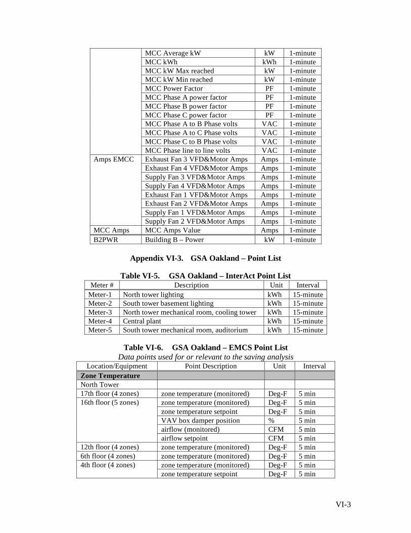
VI-3
MCC Average kW kW 1-minute MCC kWh kWh 1-minute MCC kW Max reached kW 1-minute MCC kW Min reached kW 1-minute MCC Power Factor PF 1-minute MCC Phase A power factor PF 1-minute MCC Phase B power factor PF 1-minute MCC Phase C power factor PF 1-minute MCC Phase A to B Phase volts VAC 1-minute MCC Phase A to C Phase volts VAC 1-minute MCC Phase C to B Phase volts VAC 1-minute
MCC Phase line to line volts VAC 1-minute Exhaust Fan 3 VFD&Motor Amps Amps 1-minute Exhaust Fan 4 VFD&Motor Amps Amps 1-minute Supply Fan 3 VFD&Motor Amps Amps 1-minute Supply Fan 4 VFD&Motor Amps Amps 1-minute Exhaust Fan 1 VFD&Motor Amps Amps 1-minute Exhaust Fan 2 VFD&Motor Amps Amps 1-minute Supply Fan 1 VFD&Motor Amps Amps 1-minute
Amps EMCC
Supply Fan 2 VFD&Motor Amps Amps 1-minute MCC Amps MCC Amps Value Amps 1-minute B2PWR Building B – Power kW 1-minute
Appendix VI-3. GSA Oakland – Point List
Table VI-5. GSA Oakland – InterAct Point List Meter # Description Unit Interval
Meter-1 North tower lighting kWh 15-minute Meter-2 South tower basement lighting kWh 15-minute Meter-3 North tower mechanical room, cooling tower kWh 15-minute Meter-4 Central plant kWh 15-minute Meter-5 South tower mechanical room, auditorium kWh 15-minute
Table VI-6. GSA Oakland – EMCS Point List Data points used for or relevant to the saving analysis
Location/Equipment Point Description Unit Interval Zone Temperature North Tower 17th floor (4 zones) zone temperature (monitored) Deg-F 5 min
zone temperature (monitored) Deg-F 5 min zone temperature setpoint Deg-F 5 min VAV box damper position % 5 min airflow (monitored) CFM 5 min
16th floor (5 zones)
airflow setpoint CFM 5 min 12th floor (4 zones) zone temperature (monitored) Deg-F 5 min 6th floor (4 zones) zone temperature (monitored) Deg-F 5 min
zone temperature (monitored) Deg-F 5 min 4th floor (4 zones) zone temperature setpoint Deg-F 5 min

VI-4
VAV box damper position % 5 min airflow (monitored) CFM 5 min
airflow setpoint CFM 5 min 2nd floor (4 zones) zone temperature (monitored) Deg-F 5 min South Tower
zone temperature (monitored) Deg-F 5 min zone temperature setpoint Deg-F 5 min VAV box damper position % 5 min airflow (monitored) CFM 5 min
16th floor (5 zones)
airflow setpoint CFM 5 min zone temperature (monitored) Deg-F 5 min zone temperature setpoint Deg-F 5 min VAV box damper position % 5 min airflow (monitored) CFM 5 min
4th floor (4 zones)
airflow setpoint CFM 5 min 2nd floor (4 zones) zone temperature (monitored) Deg-F 5 min Cooling Plant
chiller power kW 5 min chiller status on/off 5 min CHWS temperature (monitored) Deg-F 5~15 min CHWS temperature setpoint Deg-F 5~15 min CHWR temperature Deg-F 5~15 min CHW flow GPM 5~15 min CHW cooling energy Btu/h 5~15 min
Chiller CH-1~5 (5 units)
Chiller load Primary pump status on/off 5 min Secondary pump status on/off 5 min
CHW Pump CHP-1~5 (5 units)
Secondary pump VFD speed % 5 min CW Pump CP-1~5 (5 units)
CW pump status on/off 5 min
fan status on/off 5 min Cooling tower (4 units) Fan VFD (CT-1D only) % 5 min
Fan System North tower
Fan status on/off 5 min Fan VFD % 5 min Cooling valve position % 5 min Heating valve position % 5 min Differential pressure IWC 5 min Supply air temperature Deg-F 5 min Mixed air temperature Deg-F 5 min Return air temperature Deg-F 5 min
5th floor (2 cold deck fans, 1 hot deck fans, 2 return fans)
Static pressure Deg-F 5 min Fan status on/off 5 min Fan VFD % 5 min Cooling valve position % 5 min Heating valve position % 5 min
Penthouse (2 cold deck fans, 2 hot deck fans, 2 return fans)
Differential pressure IWC 5 min

VI-5
Supply air temperature Deg-F 5 min Mixed air temperature Deg-F 5 min Return air temperature Deg-F 5 min
Static pressure Deg-F 5 min South tower
Fan status on/off 5 min Fan VFD % 5 min Cooling valve position % 5 min Heating valve position % 5 min Differential pressure IWC 5 min Supply air temperature Deg-F 5 min Mixed air temperature Deg-F 5 min Return air temperature Deg-F 5 min
5th floor (2 cold deck fans, 1 hot deck fans, 2 return fans)
Static pressure Deg-F 5 min Fan status on/off 5 min Fan VFD % 5 min Cooling valve position % 5 min Heating valve position % 5 min Differential pressure IWC 5 min Supply air temperature Deg-F 5 min Mixed air temperature Deg-F 5 min Return air temperature Deg-F 5 min
Penthouse (2 cold deck fans, 2 hot deck fans, 2 return fans)
Static pressure Deg-F 5 min
Table VI-7. GSA Oakland – Submeter Point List Equipment Description Interval
CHP-NB-6 Secondary chilled water pump with VFD 1-minute CHP-NB-8 Secondary chilled water pump with VFD 1-minute SF-SP-1 South tower penthouse cold deck fan 1-minute SF-SP-2 South tower penthouse cold deck fan 1-minute SF-S5-1 South tower 5th floor cold deck fan 1-minute SF-S5-2 South tower 5th floor cold deck fan 1-minute
Trend data are 3 phases and average of kW, Amps, Power Factor and Volt.
Appendix VI-4. Roche – Point List and Fan Spot Measurement Plan
Table VI-8. Roche – PML PegaSys Point List Point Name Unit Interval
Building A2 – Whole Building Power kW 15-minute Building SS – Whole Building Power kW 15-minute Building FS – Whole Building Power kW 15-minute

VI-6
Table VI-9. Roche – Real-Time Energy Tracker Point List
Roche – Fan M&V Spot Measurement Plan (by Kris Kinney) PML - Roche is going to generate a service call with PML to have the database and time stamp reviewed and brought into current. We need to follow up on that so we can make sure that any current data is captured before the rework. More important is to determine the exact offset for the data files. There was no schedule determined on when this would be done. Building schedules: SS - Site services - Start 7 a.m. to 6 pm FS - Food Services - Starts 4:30 a.m. to 5 pm A2 - Office building - Starts 6 a.m. to 6 pm SS Building
SS AH4 Thursday 09/30/03 13:38 hours - measurement taken at MCC. Supply Fans have power factor correction capacitors. Exhaust fans did not. 5 to 7.5 kW, 480 to 490 volts, power factor (PF) 0.51, Around 30 HP motor.
SS EF 482 to 491 volts, 1380 to 1480 watts - Measurement take at disconnect at fan. Around 15 HP motor.
Category Point Name Unit Interval A2 Fan-2 Status Start/Stop 5-minute A2 Fan-4 Status Start/Stop 5-minute A2 Fan-6 Status Start/Stop 5-minute FS Supply Fan-1 Status Start/Stop 5-minute FS Supply Fan-2 Status Start/Stop 5-minute FS Return Fan-1 Status Start/Stop 5-minute
Logical Status
SS AH-04 Status Start/Stop 5-minute Equipment Status 10 Cents Plan $/kWh 5-minute Equipment Status 30 Cents Plan $/kWh 5-minute
Price Signal
Equipment Status 75 Cents Plan $/kWh 5-minute A2 SF-1,2 OSA Temperature Deg-F 5-minute A2 SF-3,4 OSA Temperature Deg-F 5-minute A2 SF-5,6 OSA Temperature Deg-F 5-minute A2 SF-1,2 Zone Temperature Deg-F 5-minute A2 SF-3,4 Zone Temperature Deg-F 5-minute
Temperature
A2 SF-5,6 Zone Temperature Deg-F 5-minute A2 SF-1,2 CO2 Concentration ppm 5-minute A2 SF-3,4 CO2 Concentration ppm 5-minute
CO2
A2 SF-5,6 CO2 Concentration ppm 5-minute

VI-7
FS Building Measurements taken on 10/15/03 at 11:00 a.m. - both fans running. Supply Fans have power factor correction capacitors. Exhaust did not.
FSSF01 Fan 4S-1 Voltage 510V, 12.3 to 12.5 kW, PF = .87, no vfd control, Around 25 HP. FSSF02 Fan 4S-2 Voltage 500 to 507V, 12.8 kW, PF = .78, no vfd control, Around 25 HP. Common exhaust Fan FE-1 Volts = 500, 5.4 kW, PF = 0.58 This fan is not interlocked with the two supply fans. Independently controlled. FSSF01 fan in solo without FSSF02 500V, 8 to 9.1 kW, Exhaust was almost the same.
A2 Building Taken on 10/15/03 from 1 to 2 pm. Each section was done within 10 to 15 minutes.
Section 1 of three Identical fan sections installed over three wings. Supply and return are interlocked. Section 3 only had one exhaust fan. Supply fans had power factor correction and exhaust did not. No vfds for control. kW PF Volts Fan 3S-3 (A2SF03) 24.2-25.1 kW 0.66 490-496 V Fan 3S-4 (A2SF04) 27.8-28.95 kW 0.67 490V Fan 3E-3 (A2RA03) 6.5 kW 0.78 490V Fan 3E-4 (A2RA04) 4.88-4.92 kW 0.55 493-500 V Fan 3S-3 (A2SF03) ran in solo 29.88 kW 0.83 495 V Fan 3E-3 (A2SF04) ran in solo 7 kW 0.84 495V
Section 2 of three Identical fan sections installed over three wings. Supply and return are interlocked. Section 3 only had one exhaust fan. Supply fans had power factor correction and exhaust did not. No VFDs for control. kW PF Volts Fan 3S-1 (A2SF01) 18.4 kW 0.77 495 V Fan 3S-2 (A2SF02) 21.8kW 0.81 495 V Fan 3E-1 (A2RA01) 4 kW 0.50 491 V Fan 3E-2 (A2RA02) 4.36 kW 0.50 495 V Fan 3S-1 (A2SF01) ran in solo 20.9 kW 0.79 495 V Fan 3E-1 (A2RA01) ran in solo 4.4 kW 0.51 499 V

VI-8
Section 3 of three Identical fan sections installed over three wings. Supply and return at not interlocked. Supply fans had power factor correction and exhaust did not. No VFDs for control. kW PF Volts Fan 3S-5 (A2SF05) 21 kW 0.79 494 V Fan 3S-6 (A2SF06) 19.2 kW 0.83 497 V Fan 3E-5 (A2RA05) 5.2 kW 0.56 497 V Fan 3S-5 (A2SF05) ran in solo 20.6 kW 0.79 494 V Fan 3E-5 (A2RA05) ran in solo 5.1 kW 0.56 497 V
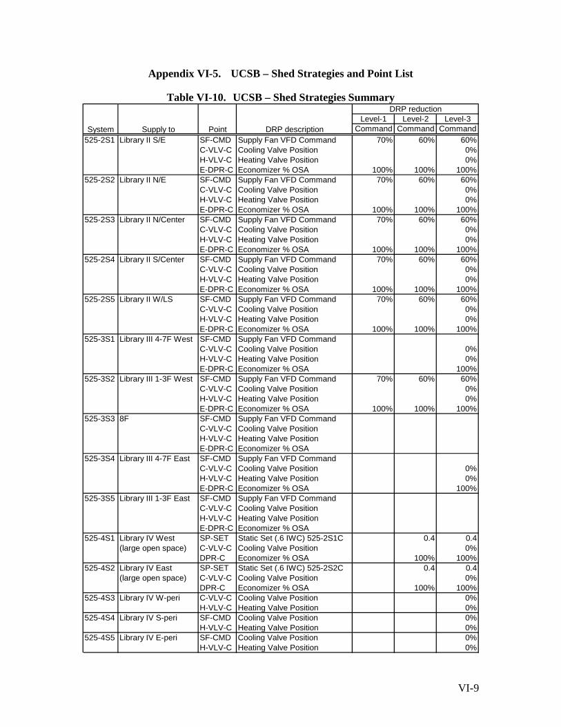
VI-9
Appendix VI-5. UCSB – Shed Strategies and Point List
Table VI-10. UCSB – Shed Strategies Summary
Level-1 Level-2 Level-3System Supply to Point DRP description Command Command Command
525-2S1 Library II S/E SF-CMD Supply Fan VFD Command 70% 60% 60%C-VLV-C Cooling Valve Position 0%H-VLV-C Heating Valve Position 0%E-DPR-C Economizer % OSA 100% 100% 100%
525-2S2 Library II N/E SF-CMD Supply Fan VFD Command 70% 60% 60%C-VLV-C Cooling Valve Position 0%H-VLV-C Heating Valve Position 0%E-DPR-C Economizer % OSA 100% 100% 100%
525-2S3 Library II N/Center SF-CMD Supply Fan VFD Command 70% 60% 60%C-VLV-C Cooling Valve Position 0%H-VLV-C Heating Valve Position 0%E-DPR-C Economizer % OSA 100% 100% 100%
525-2S4 Library II S/Center SF-CMD Supply Fan VFD Command 70% 60% 60%C-VLV-C Cooling Valve Position 0%H-VLV-C Heating Valve Position 0%E-DPR-C Economizer % OSA 100% 100% 100%
525-2S5 Library II W/LS SF-CMD Supply Fan VFD Command 70% 60% 60%C-VLV-C Cooling Valve Position 0%H-VLV-C Heating Valve Position 0%E-DPR-C Economizer % OSA 100% 100% 100%
525-3S1 Library III 4-7F West SF-CMD Supply Fan VFD CommandC-VLV-C Cooling Valve Position 0%H-VLV-C Heating Valve Position 0%E-DPR-C Economizer % OSA 100%
525-3S2 Library III 1-3F West SF-CMD Supply Fan VFD Command 70% 60% 60%C-VLV-C Cooling Valve Position 0%H-VLV-C Heating Valve Position 0%E-DPR-C Economizer % OSA 100% 100% 100%
525-3S3 8F SF-CMD Supply Fan VFD CommandC-VLV-C Cooling Valve PositionH-VLV-C Heating Valve PositionE-DPR-C Economizer % OSA
525-3S4 Library III 4-7F East SF-CMD Supply Fan VFD CommandC-VLV-C Cooling Valve Position 0%H-VLV-C Heating Valve Position 0%E-DPR-C Economizer % OSA 100%
525-3S5 Library III 1-3F East SF-CMD Supply Fan VFD CommandC-VLV-C Cooling Valve PositionH-VLV-C Heating Valve PositionE-DPR-C Economizer % OSA
525-4S1 Library IV West SP-SET Static Set (.6 IWC) 525-2S1C 0.4 0.4(large open space) C-VLV-C Cooling Valve Position 0%
DPR-C Economizer % OSA 100% 100%525-4S2 Library IV East SP-SET Static Set (.6 IWC) 525-2S2C 0.4 0.4
(large open space) C-VLV-C Cooling Valve Position 0%DPR-C Economizer % OSA 100% 100%
525-4S3 Library IV W-peri C-VLV-C Cooling Valve Position 0%H-VLV-C Heating Valve Position 0%
525-4S4 Library IV S-peri SF-CMD Cooling Valve Position 0%H-VLV-C Heating Valve Position 0%
525-4S5 Library IV E-peri SF-CMD Cooling Valve Position 0%H-VLV-C Heating Valve Position 0%
DRP reduction

VI-10
Table VI-11. UCSB – EEM Suite Point Summary Fan Trend
Interval 15-minute 5-minute
Point Category
Co
ld D
eck
Te
mp
era
ture
Co
olin
g V
alv
e C
om
ma
nd
Dis
cha
rge
Air
Sta
tic P
ress
Dis
cha
rge
Air
Te
mp
era
ture
Eco
no
miz
er
% O
SA
He
atin
g V
alv
e C
om
ma
nd
Ho
t De
ck T
em
pe
ratu
re
Re
turn
Air
Te
mp
era
ture
Re
turn
Fa
n A
mp
s
Re
turn
Fa
n k
W
Re
turn
Inle
t Va
ne
Co
mm
an
d
Re
turn
VF
D C
om
ma
nd
Su
pp
ly F
an
Am
ps
Su
pp
ly F
an
kW
Su
pp
ly V
FD
Co
mm
an
d
Zo
ne
Te
mp
era
ture
Co
olin
g V
alv
e C
om
ma
nd
He
atin
g V
alv
e C
om
ma
nd
Su
pp
ly V
FD
Co
mm
an
d
S-1 Fan 1 1 1 1 1 1 1 1 1 1 1 1
S-2 Fan 1 1 1 1 1 1 1 1 1 1 1 1
S-3 Fan 1 1 1 1 1 1 1 1 1 1 1 1
S-4 Fan 1 1 1 1 1 1 1 1 2 1
Library II
S-5 Fan 1 1 1 1 1 1 1 1 2 1
S-1 Fan 1 1 1 1 1 2 1
S-2 Fan 1 1 1 1 1 1 1 1 2 1 1 1
S-3 Fan 1 1 1 1 1 1 1 1 1 2
S-4 Fan 1 1 1 1 1 1 1 1
Library III
S-5 Fan 1 1 1 1 1 1 1 1 1 2
S-1 Fan 1 1 1 1 1 1 1 1 1 1 S-2 Fan 1 1 1 1 1 1 1 1 2 1 S-3 Fan 1 1 1 1 1 1 S-4 Fan 1 1 1 1 1 1
Library IV
S-5 Fan 1 1 1 1 1 1 Total 10 15 2 5 12 13 10 2 9 2 2 2 4 9 10 21 10 4 6
Utility Trend Library II Library II Electrical Demand 15-minute
Library 3 Gas Meter 15-minute Library III Electrical Demand 1 Fl 15-minute Library III Library III Electrical Demand 8 Fl 15-minute
Library IV Library IV Electrical Demand 15-minute Library Chilled Water Use kW 15-minute
Library Main Library Main Total 15-minute
Chilled Water Use 15-minute Chiller Plant kW 15-minute Chiller Tons 15-minute Chilled Water Return Temp 15-minute Chilled Water Supply Temp 15-minute Chiller 2 Electrical Demand 15-minute Chiller 2 Run Status 15-minute Chiller Full Load Amps 15-minute Condenser Water Return Temp 15-minute
Chiller Trend
Condenser Water Supply Temp 15-minute


VII-1
Appendix VII. Additional Result Tables and Figures
Appendix VII-1. First Day Test Results
We analyzed the first day test by the whole-building method. Table VIII-1 shows the demand savings for each fifteen minute time period derived using the whole-building method. Since GSA participation failed for the first day test, the other four sites are described here. The maximum aggregated savings was 260 kW. These savings were 11% of total 2191 kW demand and 0.30 W/ ft2. Roche achieved the largest demand saving percentage among the four sites (23%), followed by Albertsons (maximum 16% of demand saving) and UCSB (maximum 11% of demand saving). Demand saving was not identified for Bank of America for this test. Three sites out of four failed some of their shed strategies. Roche achieved all the shed strategies planned. Albertsons failed one of two strategies. UCSB failed one in three strategies. Based on the equipment trend data, Bank of America failed one of one strategy.
Table VII-12. Summary of Estimated Savings of 1st Day (Whole-Building Method) Time from 13:00 13:15 13:30 13:45 14:00 14:15 14:30 14:45 15:00 15:15 15:30 15:45 16:00 16:15 16:30 16:45
to 13:15 13:30 13:45 14:00 14:15 14:30 14:45 15:00 15:15 15:30 15:45 16:00 16:15 16:30 16:45 17:00Price signal $/kW
Albertsons WBP kW 311 294 305 311 300 302 299 309 303 288 315 327 305 312 314 327Shed kW 37 53 54 52 54 42 48 51 51 54 33 36 50 39 38 34WBP shed % 11% 15% 15% 14% 15% 12% 14% 14% 14% 16% 10% 10% 14% 11% 11% 9%Shed W/spft 0.73 1.05 1.09 1.04 1.08 0.84 0.96 1.02 1.02 1.07 0.67 0.72 1.01 0.79 0.77 0.67
Bank of WBP kW 735 744 734 733 735 731 741 724 730 760 729 720 701 693 680 663America Shed kW -13 -16 -8 -2 -4 -8 -19 -5 -10 -42 -11 -12 -1 0 1 0
WBP shed % -2% -2% -1% 0% -1% -1% -3% -1% -1% -6% -2% -2% 0% 0% 0% 0%Shed W/spft -0.06 -0.08 -0.04 -0.01 -0.02 -0.04 -0.09 -0.03 -0.05 -0.20 -0.05 -0.05 -0.01 0.00 0.01 0.00
Roche WBP kW 702 662 568 639 551 585 464 455 452 447 439 431 424 577 464 459Shed kW -31 9 79 1 73 27 123 131 131 129 130 123 124 -34 26 19WBP shed % -5% 1% 12% 0% 12% 4% 21% 22% 22% 22% 23% 22% 23% -6% 5% 4%Shed W/spft -0.16 0.05 0.41 0.01 0.38 0.14 0.64 0.68 0.68 0.67 0.68 0.64 0.64 -0.18 0.14 0.10
UCSB WBP kW 779 797 794 801 786 798 807 703 706 706 697 712 716 866 775 744Shed kW 22 3 2 -7 3 -6 -19 83 66 77 84 60 61 -72 4 35WBP shed % 3% 0% 0% -1% 0% -1% -2% 11% 9% 10% 11% 8% 8% -9% 1% 4%Shed W/spft 0.08 0.01 0.01 -0.02 0.01 -0.02 -0.06 0.29 0.23 0.26 0.29 0.21 0.21 -0.25 0.01 0.12
Total WBP kW 2527 2497 2400 2483 2371 2416 2311 2191 2191 2201 2180 2191 2145 2448 2232 2193Shed kW 15 48 127 44 126 56 133 260 238 217 236 207 234 -67 71 87WBP shed % 1% 2% 5% 2% 5% 2% 5% 11% 10% 9% 10% 9% 10% -3% 3% 4%Shed W/spft 0.02 0.06 0.17 0.06 0.17 0.08 0.18 0.35 0.32 0.29 0.32 0.28 0.31 -0.09 0.10 0.12
0.750.10 0.100.30

VII-2
0
500
1000
1500
2000
2500
3000
0:00
1:00
2:00
3:00
4:00
5:00
6:00
7:00
8:00
9:00
10:0
0
11:0
0
12:0
0
13:0
0
14:0
0
15:0
0
16:0
0
17:0
0
18:0
0
19:0
0
20:0
0
21:0
0
22:0
0
23:0
0
Who
le B
uild
ing
Pow
er [
kW]
Albertsons Bank of America Roche UCSB Whole-Building Baselline
$0.75
$0.30
Figure VII-2. Summary of All Sites (1st Day)
Albertsons implemented only their overhead light shed for the first day test. Although the whole-building method indicates maximum 54 kW of savings, the component level analysis shows 26 kW of savings in the overhead light. The EIS was programmed to disable the shed (stop polling the signal) at 3:30 pm due to the client’s request. The shed was disabled at 3:30 pm, and the overhead lights came back on. However, the shed activated again at 4:00 pm, and lasted until the end of the high price signal (the cause hasn’t been identified). The disable program was removed for the second day test.
0
50
100
150
200
250
300
350
400
450
0:00
1:00
2:00
3:00
4:00
5:00
6:00
7:00
8:00
9:00
10:0
0
11:0
0
12:0
0
13:0
0
14:0
0
15:0
0
16:0
0
17:0
0
18:0
0
19:0
0
20:0
0
21:0
0
22:0
0
23:0
0
Who
le B
uild
ing
Pow
er [
kW]
Actual Whole-Building Method Baseline Figure VII-3. Albertsons – Whole Building Power and Baseline (1st Day)
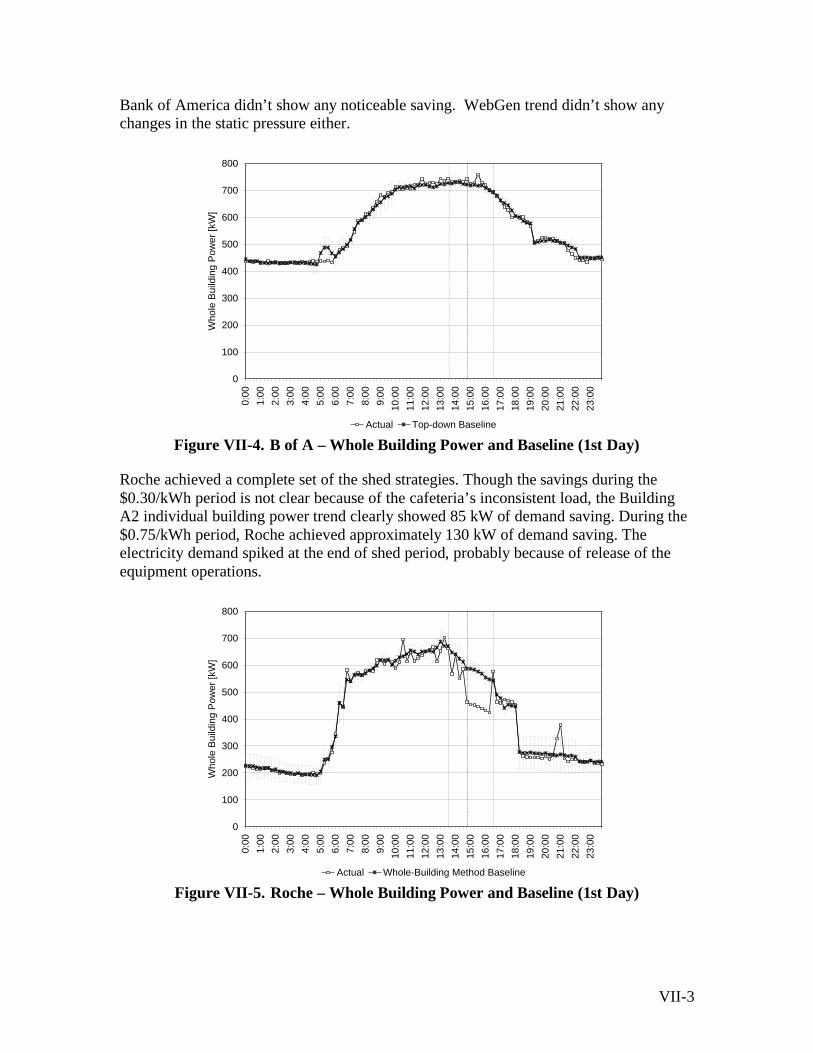
VII-3
Bank of America didn’t show any noticeable saving. WebGen trend didn’t show any changes in the static pressure either.
0
100
200
300
400
500
600
700
800
0:00
1:00
2:00
3:00
4:00
5:00
6:00
7:00
8:00
9:00
10:0
0
11:0
0
12:0
0
13:0
0
14:0
0
15:0
0
16:0
0
17:0
0
18:0
0
19:0
0
20:0
0
21:0
0
22:0
0
23:0
0
Who
le B
uild
ing
Pow
er [
kW]
Actual Top-down Baseline Figure VII-4. B of A – Whole Building Power and Baseline (1st Day)
Roche achieved a complete set of the shed strategies. Though the savings during the $0.30/kWh period is not clear because of the cafeteria’s inconsistent load, the Building A2 individual building power trend clearly showed 85 kW of demand saving. During the $0.75/kWh period, Roche achieved approximately 130 kW of demand saving. The electricity demand spiked at the end of shed period, probably because of release of the equipment operations.
0
100
200
300
400
500
600
700
800
0:00
1:00
2:00
3:00
4:00
5:00
6:00
7:00
8:00
9:00
10:0
0
11:0
0
12:0
0
13:0
0
14:0
0
15:0
0
16:0
0
17:0
0
18:0
0
19:0
0
20:0
0
21:0
0
22:0
0
23:0
0
Who
le B
uild
ing
Pow
er [
kW]
Actual Whole-Building Method Baseline Figure VII-5. Roche – Whole Building Power and Baseline (1st Day)

VII-4
UCSB failed to operate the fan VFD limit strategy. Therefore, no fan VFD-related savings could be identified during the $0.30/kWh period. UCSB succeeded with the cooling valve shed, and the whole-building method indicates a maximum savings of 84 kW. Because of release of the cooling valve, the cooling power spiked after the shed period.
0
100
200
300
400
500
600
700
800
900
1000
0:00
1:00
2:00
3:00
4:00
5:00
6:00
7:00
8:00
9:00
10:0
0
11:0
0
12:0
0
13:0
0
14:0
0
15:0
0
16:0
0
17:0
0
18:0
0
19:0
0
20:0
0
21:0
0
22:0
0
23:0
0
Who
le B
uild
ing
Pow
er [
kW]
Actual Whole-Building Method Baseline Figure VII-6. UCSB – Whole Building Power and Baseline (1st Day)

VII-5
Appendix VII-2. B of A – Result Analysis by WebGen
WebGen’s analysts independently calculated the demand savings at the B of A site using their own method. According to their calculations, Building B achieved maximum savings of 26.4 kW, and the maximum demand saving for the whole site (including the four buildings) was 199 kW (23% of the whole building power). The average demand savings for the whole site during the shed period was 8.3 %. The WebGen’s agents rotated the static pressure reset strategy across the three buildings to minimize the shed impact. The shed rotation can be clearly seen in Table VIII-3.
Table VII-13. B of A – Duct Static Pressure Change Time Bldg A Bldg B Bldg C Min SP 12:45 2.21 2.20 2.18 2.18 13:00 1.95 2.19 2.19 1.95 13:15 2.29 2.19 2.23 2.19 13:30 2.17 1.98 2.25 1.98 13:45 1.65 1.99 2.23 1.65 14:00 1.88 2.20 2.22 1.88 14:15 2.15 2.22 2.20 2.15 14:30 2.25 2.01 2.17 2.01 14:45 2.03 2.20 2.16 2.03 15:00 1.85 2.19 2.15 1.85 15:15 2.24 2.20 1.74 1.74 15:30 2.37 2.00 2.19 2.00 15:45 2.41 1.98 2.25 1.98 16:00 1.99 2.19 2.25 1.99 16:15 2.09 2.20 2.08 2.08 16:30 2.37 2.22 2.24 2.22 16:45 2.41 2.19 2.20 2.19 17:45 2.41 2.20 2.19 2.19 18:45 2.38 2.21 2.21 2.21
0.000.200.400.600.801.001.201.401.601.802.002.202.40
12:4
5
13:0
0
13:1
5
13:3
0
13:4
5
14:0
0
14:1
5
14:3
0
14:4
5
15:0
0
15:1
5
15:3
0
15:4
5
16:0
0
16:1
5
16:3
0
16:4
5
Min SP
Figure VII-7. B of A – Duct Static Pressure

VII-6
Table VII-14. B of A – Whole Building Power Saving Estimates by WebGen kW
Time Bldg A Bldg B Bldg C
Sum kW % of Mtr
12:45 0.00 0.19 2.99 3.18 0.7% 13:00 46.77 1.69 1.97 50.44 9.8% 13:15 0.00 1.04 0.00 1.04 0.2% 13:30 6.22 26.40 0.00 32.62 6.3% 13:45 94.09 25.18 0.00 119.27 23.1% 14:00 57.82 0.22 0.00 58.04 11.3% 14:15 10.53 0.00 0.69 11.22 2.2% 14:30 0.00 23.26 4.10 27.36 5.3% 14:45 27.38 0.00 5.43 32.81 7.6% 15:00 44.68 0.85 5.60 51.13 14.0% 15:15 0.00 0.38 49.22 49.60 11.9% 15:30 0.00 19.30 0.66 19.97 4.9% 15:45 0.00 18.60 0.00 18.60 5.0% 16:00 20.30 0.88 0.00 21.19 7.9% 16:15 10.82 0.05 9.12 20.00 7.4% 16:30 0.00 0.00 0.00 0.00 0.0% 16:45 0.00 0.36 0.00 0.36 0.1% 17:45 0.00 0.00 0.66 0.66 0.3% 18:45 0.00 0.00 0.00 0.00 0.0%
Average 36.66 8.3%
0.00
20.00
40.00
60.00
80.00
100.00
120.00
140.00
12:4
5
13:1
5
13:4
5
14:1
5
14:4
5
15:1
5
15:4
5
16:1
5
16:4
5
18:4
5
Sum D kW
Figure VII-8. B of A – Whole Building Power Saving Estimates by WebGen

VII-7
Appendix VII-3. GSA – Additional Figures
Individual Component Power and Baseline Baseline demand for the controllable components were calculated by using the OAT regression method. Because of the “tower free cooling” strategy, the chillers and the related equipment operation show irregular daily load shapes. Chiller demand increased during the first $0.30/kWh period, and dropped down at the beginning of the $0.75/kWh period (Figure VIII-8).
-200
-100
0
100
200
300
400
500
0:00
1:00
2:00
3:00
4:00
5:00
6:00
7:00
8:00
9:00
10:0
0
11:0
0
12:0
0
13:0
0
14:0
0
15:0
0
16:0
0
17:0
0
18:0
0
19:0
0
20:0
0
21:0
0
22:0
0
23:0
0
Pow
er [k
W]
Actual OAT Regression Figure VII-9. GSA – Chiller Power and OAT Regression Model
Fan power shows the demand reduction clearly during the shed. The OAT regression model seems higher than the actual demand (Figure VIII-9).
0
100
200
300
400
500
600
0:00
1:00
2:00
3:00
4:00
5:00
6:00
7:00
8:00
9:00
10:0
0
11:0
0
12:0
0
13:0
0
14:0
0
15:0
0
16:0
0
17:0
0
18:0
0
19:0
0
20:0
0
21:0
0
22:0
0
23:0
0
Pow
er [k
W]
Actual OAT Regression Figure VII-10. GSA – Fan Power and OAT Regression Model

VII-8
The pump power showed a demand spike at the end of the $0.75/kWh period, due to the start-up of the chillers (Figure VIII-10).
0
20
40
60
80
100
120
140
160
180
200
0:00
1:00
2:00
3:00
4:00
5:00
6:00
7:00
8:00
9:00
10:0
0
11:0
0
12:0
0
13:0
0
14:0
0
15:0
0
16:0
0
17:0
0
18:0
0
19:0
0
20:0
0
21:0
0
22:0
0
23:0
0
Pow
er [
kW]
Actual OAT Regression Figure VII-11. GSA – Pump Power and OAT Regression Model
No obvious demand savings could be identified for the cooling tower (Figure VIII-11).
-20
0
20
40
60
80
100
120
0:00
1:00
2:00
3:00
4:00
5:00
6:00
7:00
8:00
9:00
10:0
0
11:0
0
12:0
0
13:0
0
14:0
0
15:0
0
16:0
0
17:0
0
18:0
0
19:0
0
20:0
0
21:0
0
22:0
0
23:0
0
Pow
er [
kW]
Actual OAT Regression Figure VII-12. GSA – Cooling Tower Power and OAT Regression Model

VII-9
The pump power spiked at 3:00 pm due to the chiller staging-up (Figure VIII-12).
0
20
40
60
80
100
120
140
0:00
1:00
2:00
3:00
4:00
5:00
6:00
7:00
8:00
9:00
10:0
0
11:0
0
12:0
0
13:0
0
14:0
0
15:0
0
16:0
0
17:0
0
18:0
0
19:0
0
20:0
0
21:0
0
22:0
0
23:0
0
Po
wer
[kW
]
Primary chilled water pumps Condnser water pumpssecondary chilled water pumps
Figure VII-13. GSA – Pump Power
Zone Temperatures by Floor Zone temperatures were collected on nine floors. Each floor has four to five zones (see point list at Appendix IV). The zone temperature trends for each floor are presented in the following charts (Figures V111-13 through VIII-21). As a general trend, the west facing zone’s temperatures rose in the afternoon regardless of the setpoint increase. The North 2nd floor zone temperature didn’t show any obvious changes. Zone 2B1 was in heating mode during the test (Figure VIII-13).

VII-10
62
64
66
68
70
72
74
76
78
80
0:00
1:00
2:00
3:00
4:00
5:00
6:00
7:00
8:00
9:00
10:0
0
11:0
0
12:0
0
13:0
0
14:0
0
15:0
0
16:0
0
17:0
0
18:0
0
19:0
0
20:0
0
21:0
0
22:0
0
23:0
0
Zo
ne
Tem
per
atu
re [
Deg
ree
F]
2B1 (East) 2D2 (East) 2B4 (West) 2D1 (West) Figure VII-14. GSA – North Tower 2nd Floor Zone Temperature
For the North 4th floor (Figure VIII-14), the zone temperature for the west-facing zone (4D3) increased during the test, possibly because of solar gain. No significant temperature changes were found in the rest of the North 4th floor zones.
62
64
66
68
70
72
74
76
78
80
0:00
1:00
2:00
3:00
4:00
5:00
6:00
7:00
8:00
9:00
10:0
0
11:0
0
12:0
0
13:0
0
14:0
0
15:0
0
16:0
0
17:0
0
18:0
0
19:0
0
20:0
0
21:0
0
22:0
0
23:0
0
Zo
ne
Tem
per
atu
re [
Deg
ree
F]
4B7 Core 4D10 North 4D14 East 4D3 West Figure VII-15. GSA – North Tower 4th Floor Zone Temperature
For the North 6th floor (Figure VIII-15), the 6D1 zone temperature dropped during the shed. However, the range of temperatures observed were not around the heating setting point. We are not sure whether the zone was in heating mode or cooling mode.

VII-11
62
64
66
68
70
72
74
76
78
80
0:00
1:00
2:00
3:00
4:00
5:00
6:00
7:00
8:00
9:00
10:0
0
11:0
0
12:0
0
13:0
0
14:0
0
15:0
0
16:0
0
17:0
0
18:0
0
19:0
0
20:0
0
21:0
0
22:0
0
23:0
0
Zo
ne
Tem
per
atu
re [
Deg
ree
F]
6B6 (East) 6D11 (East) 6B1 (West) 6D1 (West) Figure VII-16. GSA – North Tower 6th Floor Zone Temperature

VII-12
Most of zone temperatures on North 12th floor increased during the shed (Figure VIII-16). However, they changed gradually and didn’t show clear setpoint staging based on the price signal.
62
64
66
68
70
72
74
76
78
80
0:00
1:00
2:00
3:00
4:00
5:00
6:00
7:00
8:00
9:00
10:0
0
11:0
0
12:0
0
13:0
0
14:0
0
15:0
0
16:0
0
17:0
0
18:0
0
19:0
0
20:0
0
21:0
0
22:0
0
23:0
0
Zo
ne
Tem
per
atu
re [
Deg
ree
F]
12B5 (East) 12D8 (East) 12B1 (West) 12D1 (West) Figure VII-17. GSA – North Tower 12th Floor Zone Temperature
Zone temperatures on the North 16th floor increased during the shed, but didn’t reach the assigned setpoint (Figure VIII-17).
62
64
66
68
70
72
74
76
78
80
0:00
1:00
2:00
3:00
4:00
5:00
6:00
7:00
8:00
9:00
10:0
0
11:0
0
12:0
0
13:0
0
14:0
0
15:0
0
16:0
0
17:0
0
18:0
0
19:0
0
20:0
0
21:0
0
22:0
0
23:0
0
Zo
ne
Tem
per
atu
re [
Deg
ree
F]
16B5 Core 16D12 East 16D8 North 16D2 South 16D5 West Figure VII-18. GSA – North Tower 16th Floor Zone Temperature
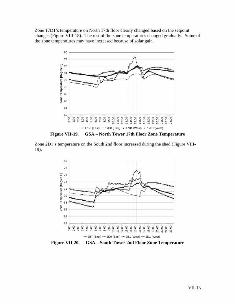
VII-13
Zone 17D1’s temperature on North 17th floor clearly changed based on the setpoint changes (Figure VIII-18). The rest of the zone temperatures changed gradually. Some of the zone temperatures may have increased because of solar gain.
62
64
66
68
70
72
74
76
78
80
0:00
1:00
2:00
3:00
4:00
5:00
6:00
7:00
8:00
9:00
10:0
0
11:0
0
12:0
0
13:0
0
14:0
0
15:0
0
16:0
0
17:0
0
18:0
0
19:0
0
20:0
0
21:0
0
22:0
0
23:0
0
Zo
ne
Tem
per
atu
re [
Deg
ree
F]
17B3 (East) 17D8 (East) 17B1 (West) 17D1 (West) Figure VII-19. GSA – North Tower 17th Floor Zone Temperature
Zone 2D1’s temperature on the South 2nd floor increased during the shed (Figure VIII-19).
62
64
66
68
70
72
74
76
78
80
0:00
1:00
2:00
3:00
4:00
5:00
6:00
7:00
8:00
9:00
10:0
0
11:0
0
12:0
0
13:0
0
14:0
0
15:0
0
16:0
0
17:0
0
18:0
0
19:0
0
20:0
0
21:0
0
22:0
0
23:0
0
Zon
e T
empe
ratu
re [D
egre
e F
]
2B7 (East) 2D9 (East) 2B1 (West) 2D1 (West) Figure VII-20. GSA – South Tower 2nd Floor Zone Temperature

VII-14
Zone temperatures on the South 4th floor did not change based on the price signal (Figure VIII-20). The temperature of the west-facing zone (4D6) increased, possibly due to solar gain.
62
64
66
68
70
72
74
76
78
80
0:00
1:00
2:00
3:00
4:00
5:00
6:00
7:00
8:00
9:00
10:0
0
11:0
0
12:0
0
13:0
0
14:0
0
15:0
0
16:0
0
17:0
0
18:0
0
19:0
0
20:0
0
21:0
0
22:0
0
23:0
0
Zo
ne
Tem
per
atu
re [
Deg
ree
F]
4B9 Core 4D10 North 4D12 East 4D14 South 4D6 West Figure VII-21. GSA – South Tower 4th Floor Zone Temperature
The south-facing zone temperatures on South 16th floor (16D11) clearly changed based on the price signal (Figure VIII-21).
62
64
66
68
70
72
74
76
78
80
0:00
1:00
2:00
3:00
4:00
5:00
6:00
7:00
8:00
9:00
10:0
0
11:0
0
12:0
0
13:0
0
14:0
0
15:0
0
16:0
0
17:0
0
18:0
0
19:0
0
20:0
0
21:0
0
22:0
0
23:0
0
Zo
ne
Tem
per
atu
re [
Deg
ree
F]
16D11 South 16D17 East 16D21 North 16B3 Core 16D5 West Figure VII-22. GSA – South Tower 16th Floor Zone Temperature

VII-15
VAV Damper Positions by Floor The VAV damper positions on the North 4th floor were not affected by the price signal, possibly due to the minimum damper position setting (Figure VIII-22).
0
10
20
30
40
50
60
70
80
90
100
0:00
1:00
2:00
3:00
4:00
5:00
6:00
7:00
8:00
9:00
10:0
0
11:0
0
12:0
0
13:0
0
14:0
0
15:0
0
16:0
0
17:0
0
18:0
0
19:0
0
20:0
0
21:0
0
22:0
0
23:0
0
VA
V D
amp
er P
osi
tio
n [
%]
4B7 Core 4D10 North 4D14 East 4D3 West Figure VII-23. GSA – North 4th Floor VAV Damper Position
The VAV damper positions on the North 16th floor seemed not to be affected by the price signal (Figure VIII-23). The PI parameter (proportional integral) setting of the south-side zone (16D8) may need to be calibrated.
0
10
20
30
40
50
60
70
80
90
100
0:00
1:00
2:00
3:00
4:00
5:00
6:00
7:00
8:00
9:00
10:0
0
11:0
0
12:0
0
13:0
0
14:0
0
15:0
0
16:0
0
17:0
0
18:0
0
19:0
0
20:0
0
21:0
0
22:0
0
23:0
0
VA
V D
amp
er P
osi
tio
n [
%]
16B5 Core 16D12 East 16D8 North 16D2 South 16D5 West Figure VII-24. GSA – North 16th Floor VAV Damper Position

VII-16
The VAV damper positions on the South 4th floor were not affected by the price signal (Figure VIII-24).
0
10
20
30
40
50
60
70
80
90
100
0:00
1:00
2:00
3:00
4:00
5:00
6:00
7:00
8:00
9:00
10:0
0
11:0
0
12:0
0
13:0
0
14:0
0
15:0
0
16:0
0
17:0
0
18:0
0
19:0
0
20:0
0
21:0
0
22:0
0
23:0
0
VA
V D
amp
er P
osi
tio
n [
%]
4B9 Core 4D10 North 4D12 East 4D14 South 4D6 West Figure VII-25. GSA – South 4th Floor VAV Damper Position
The south-side zone (16D11) VAV damper on South 16th floor changed its position to maintain the zone temperature setpoint which was changed based on the price signal. The core zone (16B3) damper position seems reduced due to the zone setpoint increase.
0
10
20
30
40
50
60
70
80
90
100
0:00
1:00
2:00
3:00
4:00
5:00
6:00
7:00
8:00
9:00
10:0
0
11:0
0
12:0
0
13:0
0
14:0
0
15:0
0
16:0
0
17:0
0
18:0
0
19:0
0
20:0
0
21:0
0
22:0
0
23:0
0
VA
V D
amp
er P
osi
tio
n [
%]
16D11 South 16D17 East 16D21 North 16B3 Core 16D5 West Figure VII-26. GSA – South 16th Floor VAV Damper Position

VII-17
Appendix VII-4. Roche – Additional Figures
Individual Building Power and Baseline OAT regression model baselines were developed for each building at the Roche site. Building A2 fan power savings could be clearly identified in the whole building power. The standard error range shows the building might have had irregular nighttime operations over the previous days.
0
50
100
150
200
250
300
350
400
0:00
1:00
2:00
3:00
4:00
5:00
6:00
7:00
8:00
9:00
10:0
0
11:0
0
12:0
0
13:0
0
14:0
0
15:0
0
16:0
0
17:0
0
18:0
0
19:0
0
20:0
0
21:0
0
22:0
0
23:0
0
Who
le B
uild
ing
Pow
er [
kW]
Actual Top-down Baseline Figure VII-27. Roche – Building A2, Whole Building Power and Baseline
The Building SS operational pattern was changed on October 30th, and the demand reduced approximately 50 kW during the afternoon (Figure VIII-27). The regression model shows higher demand than the actual demand seen on the test day because the model is affected by the demand prior to October 30th.

VII-18
0
20
40
60
80
100
120
140
160
180
0:00
1:00
2:00
3:00
4:00
5:00
6:00
7:00
8:00
9:00
10:0
0
11:0
0
12:0
0
13:0
0
14:0
0
15:0
0
16:0
0
17:0
0
18:0
0
19:0
0
20:0
0
21:0
0
22:0
0
23:0
0
Who
le B
uild
ing
Pow
er [
kW]
Actual Top-down Baseline Figure VII-28. Roche – Building SS, Whole Building Power and Baseline
Building FS’ power demand fluctuated because of electric cooking appliance use (Figure VIII-27). The spiking demand was averaged in the baseline model. Clear demand savings were obtained during the $0.75/kWh period.
0
50
100
150
200
250
0:00
1:00
2:00
3:00
4:00
5:00
6:00
7:00
8:00
9:00
10:0
0
11:0
0
12:0
0
13:0
0
14:0
0
15:0
0
16:0
0
17:0
0
18:0
0
19:0
0
20:0
0
21:0
0
22:0
0
23:0
0
Who
le B
uild
ing
Pow
er [
kW]
Actual Top-down Baseline Figure VII-29. Roche – Building FS, Whole Building Power and Baseline

VII-19
Appendix VII-5. UCSB – Additional Figures
Components Power and Baseline Cooling power dropped significantly at the beginning of the $0.75/kWh period because of the cooling valve close strategy (Figure VIII-29). However, the cooling power demand spiked up at the end of the shed period and was greater than the baseline demand for that time period.
0
20
40
60
80
100
120
140
160
0:00
1:00
2:00
3:00
4:00
5:00
6:00
7:00
8:00
9:00
10:0
0
11:0
0
12:0
0
13:0
0
14:0
0
15:0
0
16:0
0
17:0
0
18:0
0
19:0
0
20:0
0
21:0
0
22:0
0
23:0
0
Pow
er [
kW]
Actual OAT Regression Figure VII-30. UCSB – Cooling Power and OAT Regression Baseline
Although an OAT regression model was developed for the fan power, the predicted demand from the model was much lower than the actual demand around the shed period (Figure VIII-30). An alternative baseline was developed for use in determining the fan power demand savings.

VII-20
0
20
40
60
80
100
120
140
0:00
1:00
2:00
3:00
4:00
5:00
6:00
7:00
8:00
9:00
10:0
0
11:0
0
12:0
0
13:0
0
14:0
0
15:0
0
16:0
0
17:0
0
18:0
0
19:0
0
20:0
0
21:0
0
22:0
0
23:0
0
Pow
er [
kW]
Actual OAT Regression Figure VII-31. UCSB – Fan Power and OAT Regression Baseline
All of the supply fans have VFD but operated at constant volume except for the Library III – Supply Fan #2, which was operated in variable load. Because of this, the OAT regression model was applied only to this fan. Although this fan was assigned to limit the VFD% based on the price signal, it didn’t change the operation. The fan power shows that the demand spiked twice during the shed period (Figure VIII-31).
0
2
4
6
8
10
12
14
16
0:00
1:00
2:00
3:00
4:00
5:00
6:00
7:00
8:00
9:00
10:0
0
11:0
0
12:0
0
13:0
0
14:0
0
15:0
0
16:0
0
17:0
0
18:0
0
19:0
0
20:0
0
21:0
0
22:0
0
23:0
0
Pow
er [
kW]
Actual OAT Regression Figure VII-32. UCSB – 3S2-SF Demand and OAT Regression Baseline
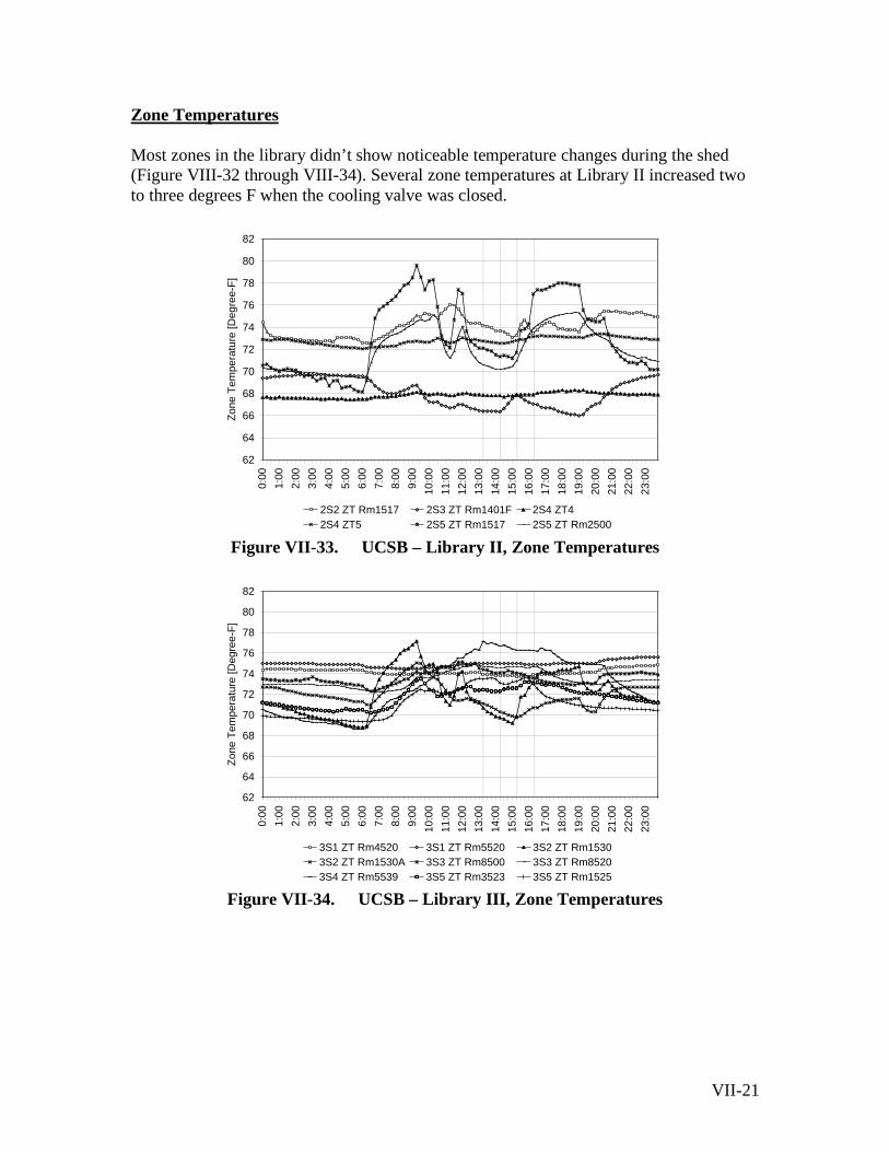
VII-21
Zone Temperatures Most zones in the library didn’t show noticeable temperature changes during the shed (Figure VIII-32 through VIII-34). Several zone temperatures at Library II increased two to three degrees F when the cooling valve was closed.
62
64
66
68
70
72
74
76
78
80
82
0:00
1:00
2:00
3:00
4:00
5:00
6:00
7:00
8:00
9:00
10:0
0
11:0
0
12:0
0
13:0
0
14:0
0
15:0
0
16:0
0
17:0
0
18:0
0
19:0
0
20:0
0
21:0
0
22:0
0
23:0
0
Zon
e T
empe
ratu
re [D
egre
e-F
]
2S2 ZT Rm1517 2S3 ZT Rm1401F 2S4 ZT42S4 ZT5 2S5 ZT Rm1517 2S5 ZT Rm2500
Figure VII-33. UCSB – Library II, Zone Temperatures
62
64
66
68
70
72
74
76
78
80
82
0:00
1:00
2:00
3:00
4:00
5:00
6:00
7:00
8:00
9:00
10:0
0
11:0
0
12:0
0
13:0
0
14:0
0
15:0
0
16:0
0
17:0
0
18:0
0
19:0
0
20:0
0
21:0
0
22:0
0
23:0
0
Zon
e T
empe
ratu
re [D
egre
e-F
]
3S1 ZT Rm4520 3S1 ZT Rm5520 3S2 ZT Rm15303S2 ZT Rm1530A 3S3 ZT Rm8500 3S3 ZT Rm85203S4 ZT Rm5539 3S5 ZT Rm3523 3S5 ZT Rm1525
Figure VII-34. UCSB – Library III, Zone Temperatures
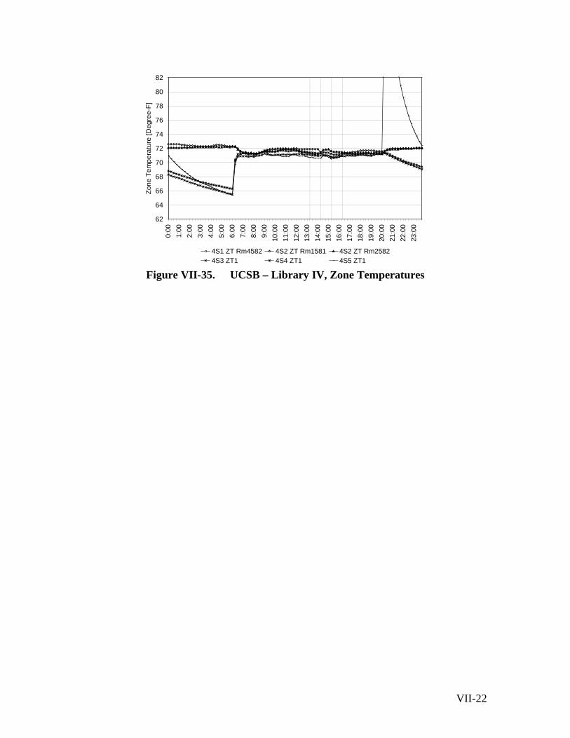
VII-22
62
64
66
68
70
72
74
76
78
80
82
0:00
1:00
2:00
3:00
4:00
5:00
6:00
7:00
8:00
9:00
10:0
0
11:0
0
12:0
0
13:0
0
14:0
0
15:0
0
16:0
0
17:0
0
18:0
0
19:0
0
20:0
0
21:0
0
22:0
0
23:0
0
Zon
e T
empe
ratu
re [D
egre
e-F
]
4S1 ZT Rm4582 4S2 ZT Rm1581 4S2 ZT Rm25824S3 ZT1 4S4 ZT1 4S5 ZT1
Figure VII-35. UCSB – Library IV, Zone Temperatures

VIII-1
Appendix VIII. Previous DR Participation and Site Contact
Appendix VIII-1. Prior Demand Response Program Participation
One of the selection criteria for participation in the LBNL tests was that each site must have demonstrated a DR capability through some DR program. Table VII-1 summarizes the programs participated, size of the curtailment capability—estimated and demonstrated.
Table VIII-15. Demonstrated Demand Response Capability of the Test Participants
Sites for final test
Facility TypeEstimated Curtailment
Capability (1) Demonstrated Curtailment
Capability (1) Pilot Test Date (1) Participation into DR Programs
Albertsons Supermarket 6.8 MW for 264 sites 5.4 MW for 264 sites 10/29/2001
CEC Peak Load Reduction Program--Demand Responsive Building Systems Element (SB5X): Subelement 2
BofALow-rise Office Building 2.8MW for 78 sites(2)
2.2 MW for 78 sites, 2.4 MW for 81 sites (3 sites added in 2003)
(3)
CEC Peak Load Reduction Program--Demand Responsive Building Systems Element (SB5X): Subelement 3. WebGen was the contractor for the award.
GSA-Oakland Federal Building Office 800 kW
800 kW (shed coordinated with SF Federal building, total of 1.2
MW from 2 M sqft) Performed during the CAISO DRP Event on July 3, 2001.
UCSB
University Campus Building 1 MW 1.1 MW 7/28/2001
CEC Peak Load Reduction Program--Demand Responsive Building Systems Element (SB5X): Subelement 2. Performed during the CAISO DRP Event on July 3, 2001.
Roche Pharmaceuticals
Manufacturing Facility 1.2 MW for 21 sites 2.5 MW for 21 sites 9/28/2001
CEC Peak Load Reduction Program--Demand Responsive Building Systems Element (SB5X): Subelement 2. Also participated in the "Cash for Kilowatts" Program. ( Offered 1.5MW within 20-minutes and delivered 2MW.)
Sites considered but not in final test
USPSMail Distribution Center 4.76 MW for 24 sites
The test during Summer 2002 was not successful. May-02
CEC Peak Load Reduction Program--Demand Responsive Building Systems Element (SB5X): Subelement 2
(1) Nexant. 2002. AB 29x and SB 5x Program Evaluation: First Quarter Report (Jan 1 to March 1, 2002 ). Page 20.(2) Communication with Don Rudy of JLL (3/11/2003)(3) Communication with John Bidwell of Nexant (3/11/2004).
Albertsons Albertsons participated in the Peak Load Reductions Program—Demand Responsive Buildings System Element as a Grantee. Albertsons participated to this program with 264 of their supermarket facilities in California. They estimated a DR capability of 6.8 MW and they were able to demonstrate load reductions of 5.4 MW at these facilities during the pilot test on October 29, 2001. The response mainly comes from reductions in anti-sweat heater energy and case lighting.
Bank of America Bank of America participated in the Peak Load Reductions Program—Demand Responsive Buildings System Element with WebGen as the Small Commercial Contractor. Bank of America participated to this program with 81 of their facilities in California. They estimated a DR capability as 2.8MW (for the initial 78 facilities—3 were added to the set in 2003) and they were able to demonstrate load reductions of 2.2 MW for the 78 original facilities (2.4 MW for the 81 facilities). The response mainly came from HVAC measures.

VIII-2
Oakland Federal Building (GSA) and 450 Golden Gate, SF (GSA) The Oakland Federal Building (Ronald Dellums Federal Building) participated in the California Independent System Operator’s (ISO) 2001 Summer Demand Reduction Program (DRP) together with the Philip Burton Federal Building in San Francisco (450 Golden Gate, SF). The demand reduction target for these two buildings was 1.2 MW. Only one curtailment (July 3, 2001) was called during the program duration (June 1 to September 30). According to ISO, 780 kW (65% of the target) was shed. However, the baseline calculation used by the ISO does not take into account the effect of temperature variation on energy use in commercial buildings. LBNL estimated that if a baseline model that accounted for temperature was used, the calculated shed would have been 120% of the target.
University of California, Santa Barbara UCSB participated in the California Independent System Operator’s (ISO) 2001 Summer Demand Reduction Program (DRP). Infotility was the load aggregator facilitating the participation. July 3rd was the only DRP event that summer. The results of the Demand Relief Program (DRP) implementation for July 3rd, 2001 from 2:00 p.m. to 6:00 p.m. show that the demand reduction was 60% of the target of 1MW. The ISO calculation for reduction is based on the previous 10 normal, non-curtailed weekdays. This baseline calculation was revised because it is not adjusted for weather conditions. July 3rd was an abnormally hot day compared to the previous weeks. The average cooling degree-days per day for the ten-day baseline was 3.7 CCD versus 6.2 CCD for July 3rd. Using the temperature-adjusted baseline, the demand reduction is calculated to be 1.1MW. UCSB also participated in the Peak Load Reductions Program—Demand Responsive Buildings System Element as a Grantee. They estimated a DR capability of 1MW and they were able to demonstrate load reductions of 1.1 MW at these facilities during the pilot test on July 28th, 2001.
Roche Pharmaceuticals Infotility has been working with the site in a PIER research project to test communications capabilities of the Infotility XML electricity price server. Roche participated in the CEC “Cash for Killowatts” program. They offered a reduction of 1.5MW within the 20-minute window that is required by the program. They were able to curtail more than 2 MW within 20-minutes of request. This qualified them for a significant grant from CEC. In addition to this they received multiple rebates from local energy provider (City of Palo Alto) for demand limiting. Three buildings at the site were chosen for the demonstration. The building chosen are A2 (administration, auditorium 101,078 ft2), SS (facility management office 67,862 ft2), and FS (cafeteria 23,159 ft2). The central plant located in the campus provides cooling energy to the buildings. Laboratory buildings were avoided for the demonstration because their airflow and indoor air quality are more carefully controlled. The buildings chosen are non-critical areas where are expected to have relatively fewer complaints. Roche participated in the Peak Load Reductions Program—Demand Responsive Buildings System Element as a Grantee. Roche participated to this program with 21 of their facilities in California. They estimated a DR capability of 1.2 MW and they were

VIII-3
able to demonstrate load reductions of 2.5 MW at these facilities during the pilot test on September 28th, 2001.
United States Postal Service (USPS) USPS participated in the Peak Load Reductions Program—Demand Responsive Buildings System Element as a Grantee. USPS participated to this program with 24 of their facilities in California—mostly distribution centers. They estimated a DR capability of 4.76 MW. The pilot tests of May 2002 were not successful primarily because the test days were cool and there was minimal cooling demand. The main DR response in these facilities was planned reduction of chiller power mainly by reducing the service level at the facility.

VIII-4
Appendix VIII-2. Interaction with Site Contacts
Albertsons LBNL first contacted Albertsons Supermarkets in February, 2003 in an effort to recruit them to participate in the DR test. Our negotiations took many months. LBNL’s communications with them was delayed by the time required to finalize the XML signal specifications and associated software requirement. Another reason for the delay is the complicated corporate structure. We tried to contact Invensys to secure the technical development for the communications. We later found out that Elutions was fully acquired by Engagenet and we needed to work with them. Our main contact at Engagenet resigned during our lengthy discussions with them leaving us where we started. During our effort to secure a site we worked with Albertsons, Engagenet, Elutions, and the Albertsons local management. During September and October activities were in two areas:
(1) We worked on securing a specific site, convincing the store management that the tests would not be too disruptive and working with the store management to develop a two level response strategy. The building selected for the test is 3000 East 9th St. in Oakland. The first site that was nominated for the test was not a good site because the whole-building electric meter was not connected to the EIS. We also needed to work with Albertsons in making hardware modifications at the site to facilitate the communication between EIS and the controls.
(2) We worked with Elutions/Engagenet for the connectivity and communication between Infotility and the EIS. For this, we needed to procure services from Infotility too.
Bank of America LBNL has been in communication with WebGen for more than one and a half years. WebGen staff visited LBNL while LBNL was conducting a review of Energy Information Systems and we have been in several meetings where they demonstrated their products to us. Through WebGen, we contacted Jones Lang LaSalle (JLL) who is the property manager for many of the Bank of America (B of A) buildings in California. We had a meeting with JLL in early March 2003 where we identified possible buildings. Bank of America was very motivated to participate in our test. Bank of America has 78 buildings that have DR capability facilitated by WebGen. Most of the buildings are branch offices. There are four buildings that are not branch offices and they vary in size form 100,000 ft2 to 500,000 ft2. As a result of our meetings with B of A, we identified the 500,000-ft2 building in San Francisco as our primary candidate. This San Francisco building is equipped with a Honeywell Energy Management Control System (EMCS). As mentioned above, the EIS on top of this system is WebGen. The San Francisco office was Webgen’s first experience connecting to a Honeywell system. We were initially concerned that this may pose a problem because when the building was recruited for the project, the gateway connectivity had not been completed. During

VIII-5
August, 2003 we were informed that the connectivity was completed and the testing could proceed. In early September, 2003, JLL and Webgen informed us that the San Francisco office building was being sold. Webgen and JLL selected the B of A’s Concord Technology Center (CTC) for the study. The CTC consists of 4 large buildings with about 1 million ft2 of space. Webgen links to a Trane Trace EMCS, and the linkage has been completed. We visited the site on September 10. During this meeting one of the four buildings (Building B) was selected as the site that would be monitored. The response strategy, the monitoring and verification methodology, and other issues related to communications were discussed. During the following weeks, we were in contact with the building operators. We worked with them during the installation of our short term metering equipment. The building operators also provided us with data from the Trane system to complement data from Webgen and our own short term metering. During late September and October WebGen completed software upgrade to accept the XML signals from Infotility, submetering was installed to verify our ability to measure the shed strategy, the list of Trane data points to be monitored were identified and LBNL obtained Webgen data files to ensure we can analyze the test results.
Bank of America, JLL, and WebGen chose a site in Concord which has four buildings (A, B, C and D) used for office and data center. Building D is a data center, and has the central cooling plant which supplies chilled water to all the four buildings. The other buildings are offices. Building B was chosen for the test, because it had no known problem such as over heating or solar gain problems. Oakland Federal Building (GSA) and 450 Golden Gate, SF (GSA) LBNL has been working with this building for several years. One project consisted of an energy assessment using EMCS trend logs, which resulted in a paper at the National Conference on Building Commissioning. A second study was conducted to assist in the development of the DR strategies. LBNL is also partnering with GSA on the development of GEMnet: GSA Energy and Maintenance Network. LBNL’s involvement in this site build’s on the multi-year relationship and collaboration with GSA and the on-site staff. University of California, Santa Barbara UCSB was the subject of an LBNL study on the cost effectiveness of Energy Information Systems (Motegi et al, 2003). This study involved interviewing Jim Dewey, the energy manager, on how he uses the EIS. Multi-year energy data were collected and specific examples of building operating problems identified with the EIS.

VIII-6
Roche Pharmaceuticals United States Postal Service (USPS) LBNL has been working with USPS through funding from Federal Energy Management Program (FEMP) for almost a decade. The Electricity Markets and Policy Group at LBNL have been leading this activity to help USPS strategize energy procurement and energy-efficiency investments. Before the DR tests during 2002, we were invited to a training session facilitated by Viron for USPC facility managers and we had a chance to meet several of the key people in this organization. At this meeting, we had a chance to introduce our project both to Viron and USPS. In order to convince USPS to participate in our test, we offered them to provide an estimate of their potential savings under the new proposed CPP tariff. USPS provided us with real time interval data for all of their facilities. Because only PG&E provided prices on their proposed CPP tariff, we analyzed the potential savings for the West Sacramento Distribution Center that is supplied by PG&E. Unfortunately our analysis did not show significant savings—especially with the delayed start day of the CPP tariff. Table VI-2 indicates that if the tariff had been available, it would be beneficial for the facility to participate. Even without any action, their gain would be around $6000. With a response of about 5%, they could have increased this benefit to about $9000. However, these profits would diminish and serious losses would take place with a delay of the program to June.
Table VIII-16. The benefits of participating in CPP tariff for a USPS distribution center in West Sacramento using load profiles from 2002($)
May June July Aug Sept Oct
June to Oct May to OctNo Action 18153 16794 -14676 -32926 924 17445 -12440 5714
5%Curtailment on CPP days during CPP on-peak hours 18153 16794 -13590 -31289 1464 17445 -9175 8978
Note: CPP days were selected as the 12 days with the highest California ISO system load in 2002
Total
In a further attempt to secure their participation, we contacted Viron to explore the possibility of synchronizing our tests with the tests USPS/Viron needed to perform during the summer as part of the Peak Load Reduction Program. At that point, Viron was very motivated to incorporate the software developed by Infotility in their system to receive XML price signals. We provided Viron with the preliminary specification of the XML signal and their technical group began working on this issue. Viron was going to help us pick the most suitable site out to the 24. Because of LBNL’s long relation with USPS, we have extensive information on each site. As mentioned, we also were given access to interval near-real-time data on all of their facilities that are of interest to us. LBNL made great progress in discussions with USPS and Viron. A postal distribution center in San Jose was selected for the test

VIII-7
because the on-site staff was supportive and interested in DR. Numerous discussions were made with USPS and the MOU was signed. During late summer, Chevron Energy Services purchased Viron. We continued numerous discussions with Bruce Dickenson, our contact at Viron. However, we were unable to proceed with the project because Chevron was upgrading the Information Technology infrastructure. They are unable to make the additional programming upgrades to the Utility Vision system at a time when the infrastructure was changing. Although USPS and Viron dropped out of the test, they are still interested in participating in any future projects.

VIII-8
Appendix VIII-3. Problems Encountered During Test Period
Several problems were encountered during the two-week test period, specifically before the initialization of the test on November 12th as well as before the November 19th test. During the two three-hour high price periods, signaling went smoothly except for a few minor problems. Table 4-2 summarizes the kinds of problems encountered.
Table VIII-17. Problems Encountered During The 2-Week Test Period Albertsons B of A GSA Roche UCSB Tuned into wrong channel Not confirming Signaled unsuccessful data transfer Time stamp discrepancies Programmed delay in confirmation signal
Action premature (before price in effect)
Signal confirmed > 2 minutes from time published
All of these problems are start-up problems and could be eliminated with proper commissioning. We do not anticipate that these will cause long term issues and/or bottlenecks. The rest of this section provides a more detailed accounting of these problems. One issue to note is that all of these problems were resolved before the second Auto-DR test on November 19th, 2003.
Albertsons
Polling wrong channel. A private test channel was set-up for each site for use prior to the official test window. During the official test window, the sites switched over from their private test channel to the official LBNL “production” channel. Albertsons polled their private test channel in addition to the production channel until November 12th at 12:45 pm. LBNL observed this discrepancy and the problem was corrected minutes before the first Auto-DR test. Not Confirming. During the two-week test period, 110 signals were not confirmed. The signal was not confirmed once at 10:30 pm on November 13th. Confirmation stopped totally between November 17th at 4:15 p.m. and November 19th at 9:00 am. See Table 4-3 for part of this time period’s communication log. Corrections were made just before the second Auto-DR test.

VIII-9
Table VIII-18. Signal Not Being Confirmed - Albertson
ChannelID Channel Description
UserID UserName When requested by user
Timestamp [asc]
Price sent by server
Price returned by user
When returned by user
1233 Price_LBNL1 397 albertsons,cpu1_ 11/19/2003 8:47:10 AM
11/19/2003 9:00:00 AM
0.1
1233 Price_LBNL1 397 albertsons,cpu1_ 11/19/2003 9:02:09 AM
11/19/2003 9:15:00 AM
0.1 0.1 11/19/2003 9:20:27 AM
Bank of America
Polled wrong channel and premature action. The Bank of America site tested their systems on the afternoon of November 1st. Although the test started at 6:00 pm on November 11th they did not start to listen to any channel until 7:00 am on November 12th. At that point they started sending requests to their own test channel and not the LBNL-channel. The problem was corrected at 8:30 am on November 12th when they started requesting to the proper test channel.
GSA
Not confirming, time stamp discrepancies, programmed delay in confirmation signal, action premature and signal confirmed > 2 minutes. On three separate days over the two week test period, a total of 35 signals were not confirmed by the GSA system: November 11th (9:45 am to 5:30 pm), November 12th (1:45 pm when the signal switched to $0.30/kWh and 3:15 pm when the signal was $0.75/kWh), November 18 (10:15am), and November 21st (11:00 am). At the beginning of the two week test period, the GSA confirmation stamp was about an hour later than the time stamp of the signal and receipt time stamps. This problem was due to the time difference between the different servers involved and was corrected on November 11th at 5:30 pm. Signals were confirmed in greater than two minutes from the time they were published, until approximately the time when the price took effect—13 to 15 minute delay from the time the signal was received.
Roche
No problems were noticed during the two-week test period. Signals were requested in less than two minutes from the time they were published. Signals were confirmed within two minutes from the time they were requested.
UCSB
Thirteen Unsuccessful data transfer and action premature. Signals were received incorrectly during the two week test period, some on November 10th and some on

VIII-10
November 11th (See Table 4-4). The problem was corrected by 11:00 am on November 11th.
Table VIII-19. Participant Returning Wrong Value for the Signal - UCSB
ChannelID Channel Description
UserID UserName When requested by user
Timestamp [asc]
Price sent by server
Price returned by user
When returned by user
1233 Price_LBNL1 385 ucsb,cpu1_ 11/10/2003 9:30:43 AM
11/10/2003 9:45:00 AM
0.1 -1 11/10/2003 9:46:05 AM
1233 Price_LBNL1 385 ucsb,cpu1_ 11/10/2003 9:46:05 AM
11/10/2003 10:00:00 AM
0.1 0.1 11/10/2003 9:47:07 AM