Developing High-Frequency Equities Trading ModelsBy

Leandro Rafael InfantinoB.Sc. Industrial Engineering

Instituto Technologico De Buenos Aires(ITBA), 2004

BySavion Itzhaki

B.Sc. Electrical Engineering /B.A. PhysicsTechnion - Israel Institute of

Technology, 2006

SUBMITTED TO THE MIT SLOAN SCHOOL OF MANAGEMENT IN PARTIALFULFILLMENT OF THE REQUIREMENTS FOR THE DEGREE OF

MASTER OF BUSINESS ADMINISTRATION MASSACHAT THE OF1

MASSACHUSETTS INSTITUTE OF TECHNOLOGY

June, 2010LIE

©2010 Leandro R. Infantino and Savion Itzhaki. All rights reserved.

ARCHIVESUSETTS INSITuTEECHNOLOGY

N 0 8 2010

RARIES

The author hereby grants to MIT permission to reproduce and to distribute publicly paper andelectronic copies of this thesis document in whole or in part in any medium now known or

. , ereafter created.

Signature of Author:

,r) /7,/

Signature of Author:

Leandro R. InfantinoMIT Sloan School of Management

May 7, 2010

Savion ItzhakiMIT Sloan School of Management

May 7, 2010

Certified by:Roy E. Welsch

Professor of Statistics and ManagementScience and Engineering Systems

Thesis AdvisorAccepted by:

Debbie BerechmanExecutive Director, MBA ProgramMIT Sloan School of Management

Developing High-Frequency Equities Trading Models

ByLeandro Rafael Infantino and Savion Itzhaki

Submitted to the MIT Sloan School of Managementon May 7, 2010 in Partial Fulfillment of the

Requirements for the Degree of Master of Business Administration

Abstract

The purpose of this paper is to show evidence that there are opportunities to generate alpha in

the high frequency environment of the US equity market, using Principal Component Analysis

(PCA hereafter) as a basis for short term valuation and market movements prediction. The time

frame of trades and holding periods we are analyzing oscillate between one second to as high as

5 minutes approximately. We particularly believe that this time space offers opportunities to

generate alpha, given that most of the known quantitative trading strategies are implemented in

two different types of time frames: either on the statistical arbitrage typical type of time frames

(with valuation horizons and trading periods in the order of days or weeks to maybe even

months), or in the purely high frequency environment (with time frames on the order of the

milliseconds). On the latter strategies, there is really not much intention to realize equity

valuations, but rather to benefit from high frequency market making, which involves not only

seeking to earn profit from receiving the bid/ask spread, but also from the transaction rebates

offered by the numerous exchanges to those who provide liquidity. We believe that there are

more opportunities to capture existing inefficiencies in this arena, and we show how with very

simple mathematical and predictive tools, those inefficiencies can be identified and potentially

exploited to generate excess returns. The paper describes our underlying intuition about the

model we use, which is based on the results of short term PCA's on equity returns, and shows

how these results can predict short term future cumulative returns. We randomly selected 50 of

the most liquid equities in the S&P 500 index to test our results.

Thesis Supervisor: Roy E. WelschTitle: Professor of Statistics and Management Science and Engineering Systems

Acknowledgments

We would like to thank all of those who helped throughout the thesis write-up. We would like to

start by thanking Prof. Roy E. Welsch for being our advisor in this thesis, for all of his guidance

and support, and for presenting us with this unique opportunity to work with him.

We also thank Prof. Jun Pan, Prof. Leonid Kogan, and Mark T. Mueller of MIT for helpful

comments and discussion throughout the process.

Finally, our special thanks goes to Neil Yelsey from QCap LLC. This thesis would not have

been possible without the Neil great devotion to this process. Neil has shared with us a great

amount of time and resources for this thesis and has been a real mentor.

Contents1 INTRODUCTION .................................................................................. ............. 8

1.1 DESCRIPTION OF THE PROBLEM ....................................................................................................... 8

1.2 AVAILABLE SOLUTIONS.. .ARE THERE ANY? ............................... . . . . . . . . . . . . . . . . . . . . . . . . . . . . . . . . . . . . . . . . . . . . . . . . . . 12

2 THE M ODEL ........................................................................................................... 18

2.1 THE BENEFITS OF USING LOG RETURNS ....................................................................................... 18

2.2 THE USE OF PRINCIPAL COMPONENT ANALYSIS ................................................................. 20

2.3 THE USE OF CUMULATIVE RETURNS ....... .................................................................................. 22

2.4 DESCRIPTION OF THE MODEL ....................................................................................................... 23

2.5 SIMPLIFYING ASSUMPTIONS......................................................................................................... 29

2.6 BASIC MODEL RESULTS................................................................................................................ 30

3 REGIM E SW ITCHING M ODEL .............................................................................. 41

3.1 DESCRIPTION OF THE MODEL ....................................................................................................... 41

3.2 REGIME SWITCHING MODEL RESULTS...........................................................................................52

4 POTENTIAL IM PROVEM ENTS..............................................................................53

4 .1 C LU STERIN G .................................................................................................................................. 53

4.2 SELECTION OF EIGENVECTORS........................................................................................................54

4 .3 N L S .............................................................................................................................................. 5 6

4 .4 O TH ER ........................................................................................................................................... 57

5 CONCLUSION ............................................................................................................ 58

REFERENCES ................................................................................. 59

1 Introduction

1.1 Description of the problem

The problem we want to solve is a long lived dilemma that traders, asset managers, insurance

companies, banks, private investors and even any human being would be more than happy to

solve, because a deterministic closed form type of solution would simply mean infinite wealth to

whomever discovers it. The problem we want to solve is twofold:

(i) A short term security valuation problem.

(ii) A regime identification problem, to understand if the market will act either in line, or

opposite of our valuation.

In particular, we want to build a predictive model to estimate future returns on US equities on a

high frequency environment, with approximate holding periods on the order of seconds to

minutes, to exploit a quantitative signal driven trading strategy. We are more than aware of the

challenge we face, and before trying to describe how we plan to address it, we want to ensure we

completely understand what type of problem and challenge we are dealing with.

We firmly believe that the recent paper written by Mark Mueller and Andrew Lo

("WARNING: Physics Envy May Be Hazardous To Your Wealth!" - March 2010) describes

very clearly the dilemma on how to understand the spectrum of challenges involved in solving

problems in finance and economics. They demonstrate that the systematic quantitative approach

(typical of hard core sciences such as physics) used to solve finance and economics problems

over time have led to significant advances. However, completely relying on it can lead to

dangerous pitfalls.

They defined taxonomy of uncertainty in to 6 levels of risk:

(i) "Level 1: Complete Certainty" ... "All past and future states of the system are determined

exactly if initial conditions are fixed and known-nothing is uncertain."

(ii) "Level 2: Risk without Uncertainty" ... "No statistical inference is needed, because we

know the relevant probability distributions exactly, and while we do not know the

outcome of any given wager, we know all the rules and the odds, and no other

information relevant to the outcome is hidden."

(iii)"Level 3: Fully Reducible Uncertainty" ... "situations in which randomness can be

rendered arbitrarily close to Level-2 uncertainty with sufficiently large amounts of data

using the tools of statistical analysis."

(iv) "Level 4: Partially Reducible Uncertainty" ... "situations in which there is a limit to what

we can deduce about the underlying phenomena the data. Examples include data-

generating processes that exhibit: (1) stochastic or time-varying parameters that vary too

frequently to be estimated accurately; (2) nonlinearities too complex to be captured by

existing models, techniques, and datasets; (3) non-stationarities and non-ergodicities that

render useless the Law of Large Numbers, Central Limit Theorem, and other methods of

statistical inference and approximation; and (4) the dependence on relevant but unknown

and unknowable conditioning information."

(v) "Level 5: Irreducible Uncertainty" ... "This type of uncertainty is the domain of

philosophers and religious leaders, who focus on not only the unknown, but [also] the

unknowable."

(vi)"Level o: Zen Uncertainty" ... "Attempts to understand uncertainty, are mere illusions;

there is only suffering."

The taxonomy is better illustrated by applying it to two problems: one from physics, the

harmonic oscillator, and one from Finance, an equity market-neutral mean-reversion trading

strategy. This simple illustration shows very clearly that when we introduce complexity to a

physics problem and take it to a higher level of uncertainty, solutions become non trivial and

extremely difficult. Analogously, when applying the same concepts on a very basic finance

problem, where complexities do not have to be added artificially but simply exist in its nature,

the problem shows the same level of challenges if tried to solve by a concise purely quantitative

"physics" type of solution, as the first oscillator problem when taken to high levels of

uncertainty. This paper shows how the uncertainties we usually deal with in finance problems are

on the higher levels, and therefore demonstrates how solving those problems with quantitative

techniques is extremely challenging. We are very conscious of this challenge, and writing this

paper simply helps us to understand that if we plan to solve a problem in finance through

quantitative methods and expect a high level of precision in the solution, we have extremely high

expectations.

The good news is that in the environment we are dealing with, we don't care very much

about high precision. To generate alpha in a high frequency environment, using a large number

of securities and trading periods, we don't need to be extremely precise. We only need to be

slightly precise to generate decent alpha. To better illustrate this idea, we want to recall the

concept brought by Grinold and Kahn in their book "Active Portfolio Management". In

particular we want to recall the Fundamental Law of Active Management, which tells us that the

Information Ratio (IR) 1 on a trading strategy, is approximately proportional to the InformationCoefficient (IC) and to the Breadth by the following relationship:

IR = IC VBreadth

where the IC is defined as the coefficient expressing our skill, or the quality of our investmentdecisions, and the "breadth" is the number of independent decisions made on a trading strategyin one year, or also defined as "the number of independent forecasts of exceptional return wemake per year". The IC should be computed as the correlation between the forecasts and theactual outcomes, by definition.

Let's build a numerical example to identify the advantage of operating in the high frequencyenvironment. Let's assume that a certain "star" portfolio manager manages a portfolio of the 500stocks on the S&P 500. This seems like a reasonable number in order to be able to followresponsibly all the fundamentals driving the prices of all the stocks, with the assistance of hisgroup of analysts, along the time. Let's also assume that based on his analyses he makes around350 independent decisions every year on his portfolio. This means that he trades 350 times in hisportfolio over a year, representing a bit more than one trade per day, either for rebalancing,buying, selling or shorting his stocks. For somebody aiming at a holding period of 2 to 5 yearsper stock, this number of stocks and the number of independent decisions seem reasonable.Translating this into Grinold's and Kahn's concept, this portfolio manager's strategy has aBreadth of 350. Assuming he has an IC = 0.05 (which represents a very high skill and quality ofinvestment decisions), we expect him to obtain an Information Ratio of 0.93. This is a hugeInformation Ratio, representative of a traditional low frequency portfolio manager who has suchan impressive IC as this one; remember this is the "star" portfolio manager. Now imagine asimple high frequency trader, who works by himself and designs a quantitative trading strategyon 3000 of the most liquid stocks in the US market. His strategy, just like ours, updates a tradingsignal every second on the 3000 stocks. There are 23,401 seconds in a trading day, and5,873,651 on a year. Assuming the trading strategy has average holding periods of 100 secondsper stock, each stock trades around 234 times per day. Considering the 3000 universe of stocksand 251 trading days per year, the Breadth is equal to 176,202,000. To achieve an Information

IR is defined as the ratio of residual return to residual risk. The residual return is the excess returns over abenchmark (e.g. S&P 500 index), and the residual risk is the standard deviation of that excess return. It's a similarconcept to the Sharpe Ratio (where the benchmark is the risk free rate), but from a strict asset managementperspective where it is more common to analyze everything from a "benchmark" perspective.

Ratio similar to the "star" portfolio manager, this single-member team high frequency trader,

only needs to achieve an IC lower than 0.00008, which means he can be 13,000 times less

precise in his estimations than his low frequency peer! This is impressive! This reality has

encouraged us to try to attack the problem we have been discussing, given that the high

frequency environment allows us to be much less precise and still generate very attractive excess

returns. We totally agree and understand the magnitude of the challenges that Mueller and Lo

presented in their paper, so we tried to play in a world where the lack of possibilities to build

precise quantitative models was not a restriction to generate decent alpha; we wanted to play in a

world where "Physics Envy" was not so "Hazardous to our Wealth".

One important feature of the problem we want to solve is to try to predict opportunities that

arise from dislocations of a stock from its fair value, and trade on the expectation that it will

mean-revert 2. Knowing that most of the high frequency traders operate on the range of the

milliseconds and mainly try to predict movements in prices on liquid stocks just to be able to

place the right bids and asks and get rewarded with exchange rebates and bid ask spreads, we can

only assume that they are not very much focused on predicting a fair value of the stocks they are

trading, but rather try to earn profits by providing liquidity3 . This fact motivates us to think that

if any mispricing arises in the high frequency environment, the "ultra high frequency" 4 traders

are probably not going to arbitrage it away, given their holding periods are shorter, and given

that it is not in their interest to obtain profits by valuation. Let's now consider the effect

identified by the working paper done by Jakub Jurek and Halla Yang on Dynamic Portfolio

Selection on Arbitrage based on studying the mean reverting arbitrage opportunities on equity

pairs. They show how divergences after a certain threshold of mispricings do not precipitate

further allocations to arbitrage strategies, but rather reduce the allocation on these arbitrage

opportunities due to intertemporal hedging demands. This tells us in some way that when

2 We only expect this mean-reversion under conditions where momentum signal is not strong enough to cancelthe strength of this mispricing. We address in section 3.1 how we take into consideration a regime shift in theenvironment that we are analyzing as an aggregate, which in return affects the significance or validity of the meanreversion signal we observe and base our trades on.

3 A big issue that arises when observing the high frequency trading world is that the information that isavailable in the exchanges regarding liquidity and depth of book are highly disturbing. Many quotes may havehidden volumes in their bid/ask quotes. So for instance, if an investor looks to by stock A and sees an ask price of$10 for the amount of 100 shares, it could most possibly be that there is a much larger quantity hiding behind thisquote of 10000 shares or even more. Not only can a trader hide his volume of the trade but also hide the quote alltogether. This means that the information available is at times misleading and therefore high frequency traders tendto test the market and "game" other traders in order to get a better picture of the real information, and make theirprofits based on their ability to interpret this information. One may say it almost as if they are playing poker.

4 These are traders that have latencies below one millisecond from the moment they receive a signal from themarket till the time they execute the trade. This arena is mostly driven by technology.

mispricings are large enough to further break through this mispricing threshold, arbitrageopportunities grow exponentially because the allocations to this strategies tend to diminish, evenwhen the dislocations grow. If we try to translate this concept just intuitively to the highfrequency world, we would analogously see that if some traders who are playing in themillisecond environment face big price dislocations in the stocks they are trading, thesedislocations are very likely to be partially exploited in the ultra high frequency world because ofthe higher trading frequency of these players. The part of the dislocation that was not "pickedup" by the ultra high frequency traders would then become available for lower frequencyplayers, who in turn may benefit from a further dislocation beyond the threshold. This willadditionally enhance a reduction in any possible existing allocations to the arbitrage (assumingthe effect described on the paper can be translated to the high frequency environment.) As Jurekand Yang put it: "Consequently, risk-averse arbitrageurs (y > 1) who face infrequentperformance evaluation... "(in our analogy us: high frequency second to minute players) "...are

redicted to be more aggressive in trading against the mispricing than equally risk-aversearbitrageurs who face more frequent performance evaluation." (In our analogy: ultra highfrequency traders.) Given there are not many players in the environment we chose to trade, andthat most players fall in the millisecond environment, we conclude that any possible arbitrageursin this higher frequency environment are likely to become less aggressive to opportunities giventhey face "more frequent performance evaluations" in their algorithms. In addition, if theseopportunities appear in our second to minute environment, they may do in an exponentiallyhigher magnitude due to the allocation reduction effect. This simple analogy motivates us tothink there are more potential reasons to operate on the trading frequencies we chose.

1.2 Available Solutions... are there any?

Our plan was to explore available solutions to the problem we want to solve, and only then buildon them our proposed solution. Not surprisingly we didn't find much about it. In particular wedidn't find anything. So our further question was: are there no available solutions to ourproblem? The answer is yes. There are. But as every single trading strategy on the financialindustry, they are kept under strict secret as part of proprietary information of those who exploitthem.

For example, the results of the Medallion Fund of Renaissance Technologies LLC show

some clear evidence that there are people who have been successful in building decent solutions

to predictive problems in the high frequency environment5 : 35% average annual returns since

1982. These numbers are after fees, and in particular, Renaissance charges management fees of

5% and a profit participation of 36%, while all hedge funds operate on the 2%-20% fee structure.

There is no other fund in the history of financial markets that has achieved similar results. What

would we give for Mr. James Simons (Renaissance founder) to publish a paper with at least a

few of his trading strategies? However, this hasn't happened yet, and we predict with very high

confidence it will not happen any time soon.

Discouraged by the proprietary nature of high frequency trading strategies, we explored other

universes of lower frequencies, where we could find potentially applicable solutions or concepts,

that could eventually be translated to our universe of interest.

The first most basic and very illustrative example we want to use, is that used by the paper

published by Khandani and Lo in 2007 - "What happened to the quants?" - to analyze the quant

melt down of August 2007. In an attempt to explain what nobody could, which was to identify

what caused the sudden shock and the three-day simultaneous melt down of all the quantitative

driven quant shops in Wall Street, Khandani and Lo built a basic market neutral equity trading

strategy, based on the most basic concept of statistical arbitrage. The strategy consists of "an

equal dollar amount of long and short positions, where at each rebalancing interval, the long

positions consist of "losers" (underperforming stocks, relative to some market average) and the

short positions consist of "winners" (outperforming stocks, relative to the same market average).

Specifically, if wit is the portfolio weight of security (i) at date (t), then"

N11

Wit = N (Rit-k - Rmt-k) Rmt-k = 1- Rit-k

Note that this strategy positions a weight in each stock proportional to the dislocation of its

return to the market threshold, and that the aggregated stock weight adds to zero (here the name

of market neutral). This simple trading strategy implemented with k=1 day (which means that the

signal and rebalancing occurs every day, and also the "winners" vs. "losers" are evaluated daily)

delivers average Sharpe Ratios considering a null risk free rate (which in these days is nothing

too unrealistic) and avoiding transaction costs, starting at 53.87 in 1995 and ending in 2.79 in

5 The Medallion Fund's performance given here is not attributed solely to the high frequency strategies it usesbut also to other strategies and in other products as well. However, these numbers just come to illustrate why there isa strong motive in this industry not to share information on trading strategies.

2007. Although some of the stocks tested in this paper are those with highest illiquidity and

coincidentally where the greatest Sharpe Ratios come from, and therefore bias the returns to an

exaggerated upside, there are still very encouraging figures to believe on the power of statistical

arbitrage and mean-reversion trading strategies. Moreover, on the same paper, Khandani and Lo

show how simulated similar strategies on higher trading frequencies from 60 minutes to 5

minutes increase the cumulative returns in less than three months to 110% and 430%

approximately.

What we conclude from this paper is that convergence of returns to a fair measure seems

plausible and adequate, and even more as the trading frequency increases.

One very important assumption of this basic strategy that we will certainly avoid when

constructing our solution7 is that it assumes that every security has a CAPM Beta close to one, or

a covariance similar to the covariance of the wide market with itself. This is not mentioned nor

intended, but it's a natural consequence of such a strategy given it expects mean reversion to a

market threshold estimated without considering any kind of significant covariance differences,

which we know exist.

Let's assume the following situation to illustrate our observation. Two of the stocks in the

market are an oil producer and an airline. Let's also assume that these two stocks are inversely

correlated, which is intuitively reasonable given the opposite exposure of both companies to the

price of crude oil. Let's assume the price of oil goes up, and the broad market of equities has

excellent positive returns too, in one day. If the broad market had a remarkable positive shock

(more than that of crude oil) due to some macroeconomic positive announcement, we expect the

oil company to rise in price more than the airline, given that the latter is negatively affected bythe oil price shock, while the previous benefitted. In other words, we know that the covariance of

these stocks and the market are different, and therefore they have different CAPM Betas.

Nevertheless, given the broad market average return threshold increased less than the oil

company's and more than the airline's, the model will send us a signal to "long" the airline and"short" the oil company, ignoring completely that these Betas might not be close to one; and

missing the fact that given they are significantly different due to their inverse-correlation- one at

least has to be substantially different to one. We say the model ignores this because if the oil

6 Another important reference that also contributes to our motivation to explore mean reversion, as a previouscornerstone of this paper, is the paper written by Lo and MacKinley in 1990 where they show how the mean-reversion paradigm is typically associated with market over reaction and may be exploited to generate alpha.

7 This strategy has obviously been shown by Khandani and Lo only for illustrative purposes but we plan to takefrom it the valuable concepts and address those assumptions that can potentially affect results significantly on a realtrading environment.

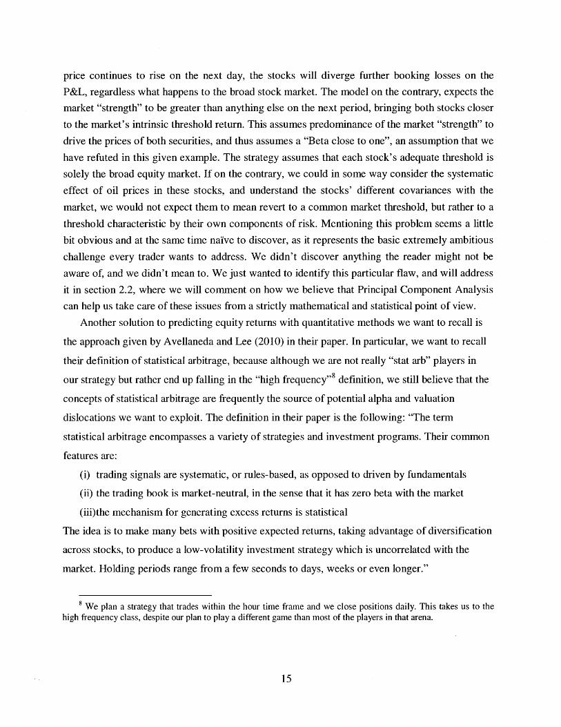
price continues to rise on the next day, the stocks will diverge further booking losses on the

P&L, regardless what happens to the broad stock market. The model on the contrary, expects the

market "strength" to be greater than anything else on the next period, bringing both stocks closer

to the market's intrinsic threshold return. This assumes predominance of the market "strength" to

drive the prices of both securities, and thus assumes a "Beta close to one", an assumption that we

have refuted in this given example. The strategy assumes that each stock's adequate threshold is

solely the broad equity market. If on the contrary, we could in some way consider the systematic

effect of oil prices in these stocks, and understand the stocks' different covariances with the

market, we would not expect them to mean revert to a common market threshold, but rather to a

threshold characteristic by their own components of risk. Mentioning this problem seems a little

bit obvious and at the same time naive to discover, as it represents the basic extremely ambitious

challenge every trader wants to address. We didn't discover anything the reader might not be

aware of, and we didn't mean to. We just wanted to identify this particular flaw, and will address

it in section 2.2, where we will comment on how we believe that Principal Component Analysis

can help us take care of these issues from a strictly mathematical and statistical point of view.

Another solution to predicting equity returns with quantitative methods we want to recall is

the approach given by Avellaneda and Lee (2010) in their paper. In particular, we want to recall

their definition of statistical arbitrage, because although we are not really "stat arb" players in

our strategy but rather end up falling in the "high frequency"8 definition, we still believe that the

concepts of statistical arbitrage are frequently the source of potential alpha and valuation

dislocations we want to exploit. The definition in their paper is the following: "The term

statistical arbitrage encompasses a variety of strategies and investment programs. Their common

features are:

(i) trading signals are systematic, or rules-based, as opposed to driven by fundamentals

(ii) the trading book is market-neutral, in the sense that it has zero beta with the market

(iii)the mechanism for generating excess returns is statistical

The idea is to make many bets with positive expected returns, taking advantage of diversification

across stocks, to produce a low-volatility investment strategy which is uncorrelated with the

market. Holding periods range from a few seconds to days, weeks or even longer."

8 We plan a strategy that trades within the hour time frame and we close positions daily. This takes us to thehigh frequency class, despite our plan to play a different game than most of the players in that arena.

As we can see we can pretty much be identified by their definition as stat arb players, but the

main difference we are going to have, is that we will not restrict ourselves to be market neutral,and we will allow the strategy to take directional market risk.

The strategy, or "ancient" solution to the problem they wanted to address, was a simple

"pairs" type of trading strategy9 based on the expectation that one stock would track the other,

after controlling adequately for Beta in the following relationship, for stocks P and Q:

In (Pt/Pto) = a(t - t o) + # In (Qt/Qto) + Xt

In its differential version:

dPf dPQt=cadt +fl + X

Pt Qt

where Xt is a mean reverting process.

Avellaneda and Lee (2010) took this concept and built a model where the analysis of

residuals generated signals that were based on relative value pricing of a sector (or cluster, as we

like to call it). They decomposed stock returns to systematic and idiosyncratic components by

using PCA and statistically modeled the idiosyncratic component. Their general decomposition

looks like this:

d~t n

=P adt + Z;flhFf + dXtPtj=1

where FU represents the risk factors of the market/cluster under consideration.

The concept of this solution is pretty similar to an important issue that we want to address

(explore mean reverting nature by using PCA) and we will definitely build our ideas of mean

reversion based on a similar behavior. Our framing of the problem will be slightly different,

given we instead want to focus on the systematic components of risk obtained from the PCA and

use them as predictive factors of future returns, by fitting an OLS model. Therefore, establishing

9 Trade expecting the convergence of a pair of stock returns on the same industry or with similar characteristics

mean reverting thresholds will be achieved by a different model. But the very basic ideas are

consequences of this "ancestor" trade as described by Avellaneda and Lee in their paper.

2 The Model

With this initial model, we only aim to solve the first part of our problem which is "short term

security valuation" described in 1.1. We do not expect significant results coming from this

strategy, because it tackles only one part of the probleml".

2.1 The Benefits of Using Log Returns

In this thesis we used log returns to build the trading signal. The use of return as opposed to the

price of the stock is much more intuitive as the return is a normalized measure. For instance,when assessing cross-sectional volatility of any universe of stocks, it is much simpler to use the

cross-sectional volatility of the returns of the stocks as they are already in a normalized form.

The prices on the other hand are drastically different in magnitude within the defined universe.

Thus in order to define thresholds for various strategies or assessment of regime changes, the

prices need to be standardized before any use can become of them which can introduce other

distortions in the model.

For example, a stock that trades at $0.50 compared to a stock that trades at $500 has very

different characteristics in regards to its liquidity, returns, trade volume, and so forth. By scaling

both stocks to the same price level, we are artificially creating two stocks that may look similar

but trade very differently. While the $0.50 stock can have a 10% return in one second of trade

(which will not be uncommon for stocks of that size), it would be very unlikely to see this kind

of move with a $500 stock.

The use of log Returns vs. real returns was done for several reasons. The main reason is that

log-returns are time additive. So, in order to calculate the return over n periods using real returns

we need to calculate the product of n numbers

(1 + r1)(1.+ r2) ... (1 + rn)

If r1 is defined as follows:

P1 -PO _ P1 P1r1 -- 1 -o 1+r 1 =-P0 PO PO

10 We will see later in section 3 how introducing a "Regime Switching" analysis attacks the rest of the problem,not attacked by the basic model analyzed in this section.

Then, the log return is defined as:

log (1 + r,) = log - = log(P 1) - log(Po)(Po

Using log returns we can easily compound the returns over n periods as follows:

log(1+r1)+ log(1+r 2)+ -+ log(1+rn) =

log + log P2 + -+ log )=LP0 P1 Pin_1)

log(P1 ) - log(Po) + log(P2) - lo9P 1 ) + -+ log(Pn) - log(Pn-1 ) =

log(Pn) - log(PO)

Thus, compounding returns is as easy as summing up two numbers.

The second reason why we used log-returns was because normality holds when compounding

returns over a larger period. For example, if we assume that r, is normally distributed, than

(1 + ri) is also normal because normality is preserved under addition. For the same reason

(1 + r2) is normal. However, (1 + r1 )(1 + r2) is not normal anymore since normality is not

preserved under multiplication.

On the other hand, assuming log(1 + ri) is normal, than log(1 + r2) is also normal. For n

period returns we can say that the total return is a linear combination of normally distributed

variables, and thus it is also normally distributed.

Another reason for the use of log-returns is that prices are log normally distributed. So,

if log (1 + r1) is a random variable with a normal distribution, then

P1 log(Pi)

PO

has a log-normal distribution. This is intuitive since prices are non-negative and can rise to

infinity, just as the log normal distribution is skewed to the right. Quoting the book

"Econometrics of Financial Markets' by Campbell, Lo and MacKinlay: " [...] problem that

afflicts normally distributed returns: violation of limited liability. If the conditional distribution

of Pt is normal, then there will always be a positive probability that Pt < 0.". This problem is

solved when taking log returns.

Finally, log returns are similar to real returns. In the high frequency space where we look at

one-second returns, the returns are fairly small and in approximation the log returns equal to the

real returns.

log (1 + r) - r , r 1

2.2 The Use of Principal Component Analysis

Principal Component Analysis is a tool of multivariate statistics widely used in engineering and

sciences to explain the main components of the variance of the many datasets involved in the

problems scientists and engineers aim to solve. PCA helps identify the drivers of variance in

chromatography analysis, image processing, medical diagnosis, soil biology, etc. The good news

is that PCA has also been widely used in finance to explain the risk drivers of diverse assets,given that one of the major variables used to explain the risk in financial assets is the variance of

their time series of returns. For example, the paper on "Statistical Arbitrage in the US Equities

Market" mentioned before (Avellaneda-Lee 2009) shows how one of the factors determining the

trading signals of their model is obtained through a PCA on stock returns. The paper shows how

PCA can play a major role in modeling risk in Finance and be used to build an alpha model. It is

over this concept - that the principal components represent an important role in determining

intrinsic risk and therefore value of securities - that we want to build on.

Instead of measuring the residual component of the stock returns, we use the principal

component for valuation using a simple linear predictive model we will describe in section 2.4.

Although our predictive method is different, and our time frames and holding periods shorter, we

still believe on the power that PCA has to explain intrinsic and fair value of financial assets, and

this concept around PCA where Avellaneda and Lee build on part of their paper, is the

cornerstone and motivation behind our trading model in the high frequency environment.

Another advantage of PCA in the time environment we are dealing with, is that traditional

fundamental factors used to determine valuation of securities for larger holding periods (months

and years) play a minor role in the valuations we are doing, and therefore, we really don't care

about the "identity" of the components of risk; we just want to capture them and ensure we

capture the relevant ones. For example, the Debt to Equity ratio, the Current Ratio, and Interest

Coverage of a company most of the time play a minor role in the price at which a certain security

will trade in the next 30 seconds. There are rather other factors affecting the high frequency

trading environment. For example, the computer driven algorithms implemented by high

frequency hedge funds, by broker dealers to execute their trades efficiently, or by asset managers

rebalancing their long term portfolios, appear to be more significant short term drivers of the

prices of securities. The factors driving these algorithms are very difficult to understand, identify

and follow using a traditional way of thinking and modeling as that of a typical equity analyst.

Using a PCA on a frequent basis seems like a more adequate tool in these cases to identify these

factors from a mathematical perspective and to update the changes in these factors as the

dynamics of the trading environment requires. The PCA will not inform us about the "identity"

of these factors as mentioned before, but we don't mind, simply because we don't care". In the

high frequency environment we only care about capturing the main factors of risk in a form that

will allow us to use them later as a predictive tool. A matrix of selected eigenvectors that can

afterwards be used to project the whole universe of stocks on a set of chosen principal

components seems intuitively more adequate to us, for building short term predictive models on

stock returns.

Another benefit of PCA is that the directions of the principal components are orthogonal by

construction. The fact that the eigenvectors of the variance-covariance matrix of returns of the

group of equities traded are orthogonal, allows us to express this time series with independent

components of risk. Although we cannot identify (at least directly) what type of risk these factors

represent, as we would on a typical low frequency fundamental based trading strategy, we are

able to determine completely that each of these factors is totally independent from one another

and represents a unique portion of uncorrelated risk of our universe. We can identify the weight

of each of these independent risk factors (by looking at their respective eigenvalues) and choose

not only how many of the independent components of risk we want to keep to build our model,

but also the amount of the total risk we are expressing with our choice. In addition, the

orthogonality property of our model will enable us to build a set of orthogonal uncorrelated

explanatory variables, more friendly to fit in a linear model, and to avoid multicollinearity.

Another important feature by PCA mentioned in the Avellaneda-Lee 2009 paper, is that it

has been used in the past in several trading strategies because it has identified risk factors

representing industry sectors without being as biased by market capitalization as other

methodologies. Translated to our world, we don't care much about identifying industry sectors,

but avoiding market capitalization bias is an important feature we would like to keep, and PCA

does that for us.

" Even if we were able to identify them, we believe that the drivers for a change in the stock price in theseconds to minutes time horizon may vary considerably at different points in time. Therefore, running a PCA in realtime will help us choose the highest risk components that are relevant for that period of time we are trading.

Finally, the last benefit of using PCA when building a mean reversion signal, is how it

addresses the flaw of the "CAPM Beta close to one" assumption of the basic equity market-

neutral strategy mentioned in section 1.2. The PCA is based on the variance-covariance matrix of

returns' 2 and therefore considers all the covariances of the stocks involved in the analysis. When

solving for principal components, this method will allow us to build a predictive model that will

determine a particular threshold for each stock, based on a different linear combination of

principal components for each of them'3 . Each of these "predicted returns" or "theoretical

returns" will have embedded in their construction all the covariance relationships of the

universe/cluster of stocks, and at the same time, will be a unique threshold for each security.

Using PCA in this way addresses the basic flaw of having to assume a general threshold for the14entire universe, with a CAPM Beta close to one for every security

2.3 The Use of Cumulative Returns

Given that we are dealing in a world where we entirely rely on mathematical models to realize

our predictions, we want to build these models to be the most possibly robust and reliable. This

is a simple and naive conclusion, but a very important one in determining the type of model we

want to build. If we are willing to build a linear model and use OLS to fit some parameters

(betas), we not only have to take care of multicollinearity and heterohedasticity in the

explanatory variables, but also must ensure that the residuals of the model are normally

distributed with mean zero and constant standard deviation. We can take advantage of the

Central Limit Theorem (CLT), and build a model to predict cumulative returns, with the

cumulative returns of the principal components. By using cumulative returns, we are using a

linear combination of stochastic variables to predict another linear combination of stochastic

variables, both normally distributed because of CLT15 . We can easily de-mean these series and

obtain a linear model with normally distributed residuals, with zero mean and constant standard

deviation, very friendly to fit in an Ordinary Least Squares (OLS) model. This is our main reason

for choosing cumulative returns in our model: to become better friends with the math, because

we need it as much as anything else to generate alpha.

12 Although it can be done by avoiding the construction of the variance-covariance matrix by a Singular ValueDecomposition approach, as described in section 4.4

13 Obtained by a simple OLS model, or by a slightly more sophisticated NLS model, both discussed in sections2.4 and 4.3 respectively

14 Flaw identified in section 1.2."5 We assume that the CLT applies here.

2.4 Description of the Model

The strategy is broken up into the following steps:

Define the stock universe: We defined a universe of 50 stocks 1. These stocks were chosen

randomly from the S&P500. We collected the top of the book bid-ask quotes on the tick data for

each trading day during 2009'7.

Ticker

GOOG

AAPL

GS

AMZN

IBM

SHLD

RL

CL

MMM

CVX

NKE

BA

XOM

JNJ

PG

SLB

PRU

BIIB

RTN

WMT

KO

TGT

HPQ

GENZ

PXD

JPM

Company Name

Google Inc

Apple Inc

Goldman Sachs Group InciThe

Amazon.com Inc

International Business Machine

Sears Holdings Corp

Polo Ralph Lauren Corp

Colgate-Palmolive Co

3M Co

Chevron Corp

NIKE Inc

Boeing Co/The

Exxon Mobil Corp

Johnson & Johnson

Procter & Gamble Co/The

Schlumberger Ltd

Prudential Financial Inc

Biogen Idec Inc

Raytheon Co

Wal-Mart Stores Inc

Coca-Cola Co/The

Target Corp

Hewlett-Packard Co

Genzyme Corp

Pioneer Natural Resources Co

JPMorgan Chase & Co

s Corp

16 The model should be adapted to a much larger universe of stocks. However, in order to work with a 1000stock universe or more, clustering techniques are very critical to have. We will discuss this point further in section4.1.

17 The top of book is the best bid and ask in the exchange. Since there are many exchanges and top of books intoday's markets, we looked at the aggregated top of book and assumed that there is no issue with liquidity or latencyto the different exchanges in order to simplify the model.

BBY Best Buy Co Inc

HSY Hershey Co/The

MRK Merck & Co Inc

ADBE Adobe Systems Inc

KFT Kraft Foods Inc

VZ Verizon Communications Inc

MSFT Microsoft Corp

MS Morgan Stanley

SUN Sunoco Inc

EBAY eBay Inc

CSCO Cisco Systems Inc

T AT&T Inc

ORCL Oracle Corp

SPLS Staples Inc

INTC Intel Corp

VLO Valero Energy Corp

GE General Electric Co

BAC Bank of America Corp

PEE Pfizer Inc

YHOO Yahoo! Inc

AA Alcoa Inc

GT Goodyear Tire & Rubber Co/The

AMD Advanced Micro Devices Inc

MOT Motorola Inc

Table 1: The 50 companies that were analyzed in the thesis and their tickers

Intervalize dataset: We intervalized the tick data to one-second intervals. This was done by

taking the first quote in each second of the trading day and calculating the mid-price.

Pmid = (Best-bid + PBest-ask)/2

The use of mid-prices was convenient for testing the strategy. In the high-frequency world, the

stocks returns as they are calculated as the change in prices that the stocks were traded, reflect

little if at all fundamental movements in the stocks and more bid-ask movements. For instance, if

a stock trades as follows: 20, 20.1, 20, 20.1, these $0.01 movements are not real returns but just

jumps between the bid and the ask. If you are competing on speed and have the technology, you

can probably capitalize on these returns. A model like ours does not compete on speed but on

valuation of the future movements of the stock in larger time frames than these tick returns.

Thus, the use of mid-prices will eliminate to a great extent the bid-ask effect, and help us

concentrate on finding alpha elsewhere. In the example above, looking at the mid-price would

show us the following: 20.05, 20.05, 20.05, 20.05, so this stock's returns will be zero since we

are seeing no movements in the stock price.

Calculate log-returns: As described in section 2.1, the use of log returns is more suitable.

Therefore we calculated the log returns on the one-second mid-prices.

PCA: We used a Principal Component Analysis in order to decrease the number of

dimensions of the dataset without losing much information along the process. The inputs to the

PCA were the log-returns that were described above. The PCA is described below:

Define,

X E RTxN

as a matrix with the time series of log returns of N stocks, for T seconds.

Define,

M E RTXN

as a matrix with the average log returns for each of the N stock in the time series in each column:

T

M = Xt , Vn E {1,2,..., N}t=1

Define,

Y G RTXN

as the de-meaned matrix of log returns of the time series 8 , where:

Y=X-M

18 De-meaned time series is the original time series minus the mean across that time series. This is important forthe PCA to work properly. Also, when calculating the variance-covariance matrix, the de-meaning is needed bydefinition: C = (X - M)T * (X - M )

Define,

Z E RNXN

as the variance-covariance matrix of Y, where:

Z YT *y

Get the eigenvectors and eigenvalues of the variance covariance matrix Z by solving:

Ex = Ax =:> | - AI| = 0

where A is the eigenvalue corresponding to eigenvector x.

Next, order the eigenvalues from largest to smallest. The largest eigenvalue is the single most

important component of risk in our universe. The more eigenvalues we choose the more risk we

are explaining in our model. Then, take the eigenvectors that correspond to the chosen

eigenvalues and place each vector in a column.

Define,

(P E R NXk

as the feature matrix with columns that are eigenvector of the variance covariance matrix E.

where N is the number of stocks, and k is the number of eigenvectors we chose to build the19feature vector.

Define,

D E RTxk

as the matrix of "dimensionally reduced returns", or principal components, obtained after

projecting Y on the principal-component plane defined by the highest k eigenvectors:

19 The number of eigenvectors that are used in the model depends on the amount of information need to buildour signal. The more eigenvectors we add the higher the precision of the model on the dataset we used to test it.However, we are risking over-fitting by using too many eigenvectors. If all eigenvectors are used, the PCA willreturn the original data set. In our model we back-tested to show that 4-5 eigenvectors (out of 50) hold over 80% ofthe risk in general and thus we used 5 eigenvectors as a fixed number to simplify this part of the model. A morecomprehensive approach can be used by using OLS techniques such as building an autoregressive model where theoptimum number of autoregressive steps are determined with a Maximum Likelihood Estimation plus a penalty fordegrees of freedom type of function (later discussed in section 4.2), to better predict the best number of eigenvectorsshould you choose to have it changing over time.

D = [tpT * YT]T

After doing the principal-component analysis, we remain with a dimensionally reduced matrix of

log returns. These dimensions hold the main components of risk in our universe of stocks.

The next step is to build a prediction model. In Campbell, Lo, and MacKinlay, ("The

Econometrics of Financial Markets," 1997), they used a log-horizon regression of stock returns

on the short term interest rates as follows:

t+1 + -- + Tt+H =l (H) y1,t - y1,t_/12 + 7t+H,H

i=0

where rt is the log return at time t, and y1,t is the 1-month treasury bill yield at time t.

This regression predicts the accumulated future H-period log returns

rt+1 + - + rt+H

by looking at an indicator that relates to the accumulated historical H-period 1-month treasury20bill yields

In our prediction model we did something similar. We calculated the accumulated future H-

period log returns. Then we ran a regression, estimated by OLS, on the future accumulated log

returns with the last sum of H-period dimensionally reduced returns in the principal component21

spaceThe results are as follows:

H H

rt+1 + '+ r't+H = f 1 t-, 1 +** ' + Yk Dt-i,k + 71 t+H,H

i=0 i=0

20 The indicator that Campbell, Lo, and MacKinlay used is actually the 1-month treasury-bill yield at time t inexcess of the mean of the historical 12 periods (including time t). However, it's a linear combination of the last 12period yields, or in approximation a sort of scale done on the accumulated returns.

21 Later we will introduce some additional terms to this regression in order to incorporate regime switching inthe prediction model, which we will compare to the current model.

Define,

B E RkXN

as a matrix that holds the betas from the regressions for all the stocks. Each of the N stocks has k

corresponding betas in the columns of matrix B.

Define,

P E RTXN

as the matrix of the new time series of the theoretical returns.

Define,

e RTXN

such that:H-1

D I Dt-i , Vt E { 1,2, -- ,T}i=0

which is a matrix that holds the accumulated historical H-period dimensionally-reduced returns

given in D.

Define,

S E R1XN

as our estimation of the accumulated (de-meaned) log-returns on the future H-periods based on

the regression that was done:

S = Dt*B

Each term in the vector S corresponds to a stock. However, in order to use this signal as a

comparison to the actual log-returns that we observe in the market, we need to add back the

original mean of the time series. Thus we will define,

S = S+Mt

as the trading signal that will be used in comparison with the prevailing log-returns in the

market. Our base assumption is that the principal components explain the main risk factors that

should drive the stock's returns in a systematic way, and the residuals as the noise that we would

like to get rid of. By using the dimensionally reduced returns, we were able to screen out much

of the noise that may have temporarily dislocated the stocks from their intended values. On this

basic mean-reversion model that does not consider regime switches, if we see that the last H-

period accumulated log-returns have been higher than the signal, we assume that the stock is

overvalued and thus place a sell order. If the opposite happens, we put a buy order. This strategy

is basically a mean-reversion strategy, since we are taking the opposite position to what has

happened in the market by assuming mean-reversion to the estimated signal. As we mentioned in

section 1.2, this is based on the same "buy losers, sell winners" concept of the equity market

neutral strategy (Khandani-Lo 2007). We want to remind the reader at this point that this model

is only solving part of our problem. We will address it completely when we include the regime

switching algorithm.

2.5 Simplifying Assumptions

One of our underlying assumptions was that we are able to buy or sell instantaneously at the mid

price. This means that once our signal tells us to buy (sell), we can execute at the same second

interval and at the mid-price. We found evidence that shows that the top of book quotes (best

bid/ask) do not change very much within the second. We also found that with these very liquid

stocks, there are usually several trades on the stock that are done in one second. So the fact that

we take the first quote at each second in the model and calculate the mid-price as our execution

price makes our assumption more realistic.

In addition to that being realistic, executing a mean-reversion strategy should position us as

market-makers. Thus, we are injecting liquidity into the system. This liquidity is a source of

income as we collect rebates plus bid/ask spread on every transaction that was executed based on

a limit order that we provided.

Another assumption we made was that transactions are made at mid-price level. This

assumption is conservative on a mean reversion liquidity providing strategy. Calculating returns

based on mid level of top of book helps mitigate the bid ask effect that is so dominant in the

space of high frequency trading. This is because the stock is not really changing value, in

between seconds. The price changes are mostly because of the market making effect of other

players in this domain.

It is important to note that if the model trades on a "momentum"2 regime, these effects

would be contrarian, and therefore we should analyze and weigh what percentage of the time the

model has been in the "momentum" and in the "mean-reversion" regimes, in order to better

understand the accuracy of the results in Sharpe Ratio, and how they might be affected by real

transaction costs.

In addition to these assumptions, we have to keep in mind that the strategy is purely

theoretical and has never been tested in the real market; it has only been tested on historical data.

We also assumed that we do not face any significant execution issues and that we are able to

execute the trades within the one-second interval where the signal was obtained. As naive as this

may sound, we believe that our strategy is very different than that of most of the high-frequency

players that are competing mainly on technology in higher frequencies, so we shouldn't be

extremely affected by our assumptions.

Finally, we assumed a time loss on computations of one second for every trading period. We

believe this to be extremely conservative.

While taking all these issues into account, it is very difficult to model these real world issues.

Building a likelihood of events could help come to a more accurate model, but it doesn't matter

how we look at it, the best way to know whether the model is working properly is by actually

trading with it.

2.6 Basic Model Results

This basic pure mean-reversion strategy has shown positive accumulated log returns in the first

quarter of year 200923, but has decreased in cumulative returns from the second quarter and all

through the end of 2009 (figure 1). The total accumulative log returns have reached -29.97% in

2009 with a very negative sharp ratio of -1.84 and volatility that resemblances the historical

average volatility of the S&P500 index (table 2).

22 'Momentum" is known as a trend following strategy, where opposed to mean-reversion, the trader expects thereturns of a security to further diverge from the established threshold, believing that it follows a trend effect drivingthe price of the security, rather than the reversion to fair value, as though by mean-reversion strategies.

23 All together there were 251 trading days in year 2009, as seen in the x-axis of the plot.

Cumulative Log Returns

30% -------- -- ----------------------------=------------

20% ------- - - - - - - - - - - - - - - - - - - - - - -

10%-------

-0%

-2 0 % -- - - - - - - - - - - - - - - - - - - - - - - - - - -

-3 0 % - - - - - - - - - - - - - - - - - - - - - - - - - - -

-4 0 % -- - - - - - - - - - - - - - - - - - - - - - - - - - -Jan Mar May Jul Sep Oct Dec

Figure 1: The plot of the accumulated log returns over a period of 251 trading days in 2009

Mean Volatility Sharpe Ratio-30.77% 16.60% -1.85

Table 2: Statistics of the strategy's performance across the entire year of 2009

In our process we recorded every single summary statistic per second for the entire year,including t-stats, betas and Rsq coefficients. Due to the impossibility to bring billions of data

points altogether, we chose instead to present what we considered very representative examples.

To illustrate the variability of the betas we picked three stocks out of the 50 tested, that

express results we believe are quite representative, and that not vary that much along the

universe from what we present here, and graphed the beta of their first principal component2 4

over the course of a day, Oct-20-2009. We did the same for the t-stats of these betas to see

whether they are statistically significant in order to check the validity of the theoretical returns

that we built based on these betas. In addition, we brought the standard deviation of each of the

five betas over the course of that day. These stocks will be referred to as "stock A", "stock B",

and "stock C".

24 "The first principal component" means the principal component that holds the highest amount of risk in theuniverse of stocks that we defined and in the trading frequency that we chose.

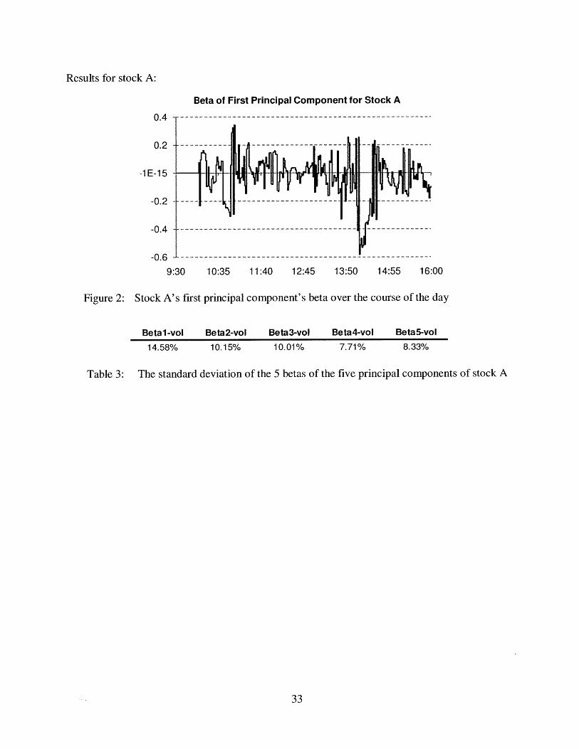
Results for stock A:

Beta of First Principal Component for Stock A

0.4 -

0.2 -

-1 E-1 5

-0.2

-0.4 ---------

-0 .6 -- - - -- - - -

9:30 10:35 11:40 12:45 13:50 14:55 16:00

Figure 2: Stock A's first principal component's beta over the course of the day

Betal-vol Beta2-vol Beta3-vol Beta4-vol Beta5-vol

14.58% 10.15% 10.01% 7.71% 8.33%

Table 3: The standard deviation of the 5 betas of the five principal components of stock A

- ---------------

----------------------

-- -----------N- -

--- -- -

------------

T-stats for Stock A

4 --- - - - - - - - - - - - - - - - - - - ----- - - - - -

3 - - - --- ------- ---- ------ - - - - - - - - - - -

2 - -- ----- --- - ------ - - - -- - -- - -

1-5

01-- --

-2 ------ ------------------ ---------- --- --- --- --- -

-3 ------ ----------------------------- --- --- ------------

-5 --- -- - - - - - - - - - - - - - - - - - - - - - - -- - -

9:30 10:35 11:40 12:45 13:50 14:55 16:00

Figure 3: T-stats for the first principal component's beta for stock A over the course of the

day

t-statsl vol t-stats2 vol t-stats3 vol t-stats4 vol t-stats5 vol136.62% 105.80% 99.92% 123.98%

Table 4: The standard deviation of the absolute value of the t-stats of the five betas for the

first five principal components of stock A

R-square for Stock A-- - - -- - - - - - - - - - - - - - - - - - - - - - -35%

30% -

25% -

20%

15%

10%

5%

0% -

9:30 10:35 11:40 12:45 13:50 14:55 16:00

Figure 4: R-square coefficient for stock A over the course of the day

Results for stock B:

Beta of First Principal Component for Stock B

0.4 -

0.2 ------ -- ------------- - - ------ -

-1E-15

-0.2

-0.4 -

9:30 10:35 11:40 12:45 13:50 14:55 16:00

Figure 5: Stock B's first principal component's beta over the course of the day

Betal-vol Beta2-vol Beta3-vol Beta4-vol Beta5-vol12.21% 8.99% 10.84% 8.11% 8.45%

Table 5: The standard deviation of the five betas of the 5 principal components of stock B

T-stats for Stock B

4 --

3 -- - - - - - - - - - - - --- ----- - - - - - - -

2 ------------ -- - - - - - ---- --------- - -------

1 - ------- -- - ---- - - - - - - - - - -

0 -

-2 ----------- - --------- ---- ------- -- - -

-3 --- - - --- ---- -- - - - -- - - - - -- - - - - -

-4 -1- - - - - - - - - - - - - - - - - - - - - - - - - - - -

-5 ------------------------------9:30 10:35 11:40 12:45 13:50 14:55 16:00

Figure 6: T-stats for the first principal component's beta for stock B over the course of the

day

t-statsl voI t-stats2 vol t-stats3 vol t-stats4 vol t-stats5 vol118.29% 85.43% 119.31% 98.31% 124.07%

Table 6: The standard deviation of the absolute value of the t-stats of the five betas for the

first five principal components of stock B

R-square for Stock B

35%

30%

25%

20%

15%

10%

5%

0% -

9:30 10:35 11:40 12:45 13:50 14:55 16:00

Figure 7: R-square coefficient for stock B over the course of the day

Results for stock C:

Beta of First Principal Component for Stock C

0.6

0 4 10:35-11:40- 12:45-- --13:50 1:1 0

0.2 -

0

-0.4

-0.6 ---- - ---08V - -- - -- -- -- --- - - - - -

9:30 10:35 11:40 12:45 13:50 14:55 16:00

Figure 8: Stock C's first principal component's beta over the course of the day

Betal-vol Beta2-vol Beta3-vol25.35% 15.03% 15.43%

Beta4-vol14.47%

Beta5-vol16.74%

Table 7: The standard deviation of the five betas of the 5 principal components of stock C

T-stats for Stock C

4 ---

3 ------------------ --- - ---- --- -- ------------------

-2 - -- -A - -- --- ----- -- -- ---3- ----- - -

-4 --

- -- - - --5 - -- - - - - - - - - - - - - - - - - - - - - - - - -

9:30 10:35 11:40 12:45 13:50 14:55 16:00

Figure 9: T-stats for the first principal component's beta for stock C over the course of the

day

t-stats1 vol t-stats2 vol t-stats3 vol t-stats4 vol t-stats5 vol137.40% 88.12% 96.62% 104.51% 133.14%

Table 8: The standard deviation of the absolute value of the t-stats of the five betas for the

first five principal components of stock C

R-square for Stock C----------- --- ---- --- ---- --- ---- --- ------35% -

30% -

25% -

20% -

15% --

10% --

5% --

0% -

9:30 10:35 11:40 12:45 13:50 14:55 16:00

Figure 10: R-square coefficient for stock C over the course of the day

Beta for the Principal Component of all stocks in October 20th 2W09

5 50 15 2

x 10 4 05 0 a 515 2

Tine in seconds Stock

Figure 11: 3D plot of Beta for the principal components of all stocks in October 20 2009

0.5 -

0 -

-1

Beta for the Puincipal Component of all stocks in October 20th 209

2 1.5 1Tire in seconds

i I I I i i i0.5 0 5 10 15 20 25

Stock

I I I 1 13 35 40 45 W0

Figure 12: Slice of Figure 11 to visualize the range of the Beta values

2.5

x 10

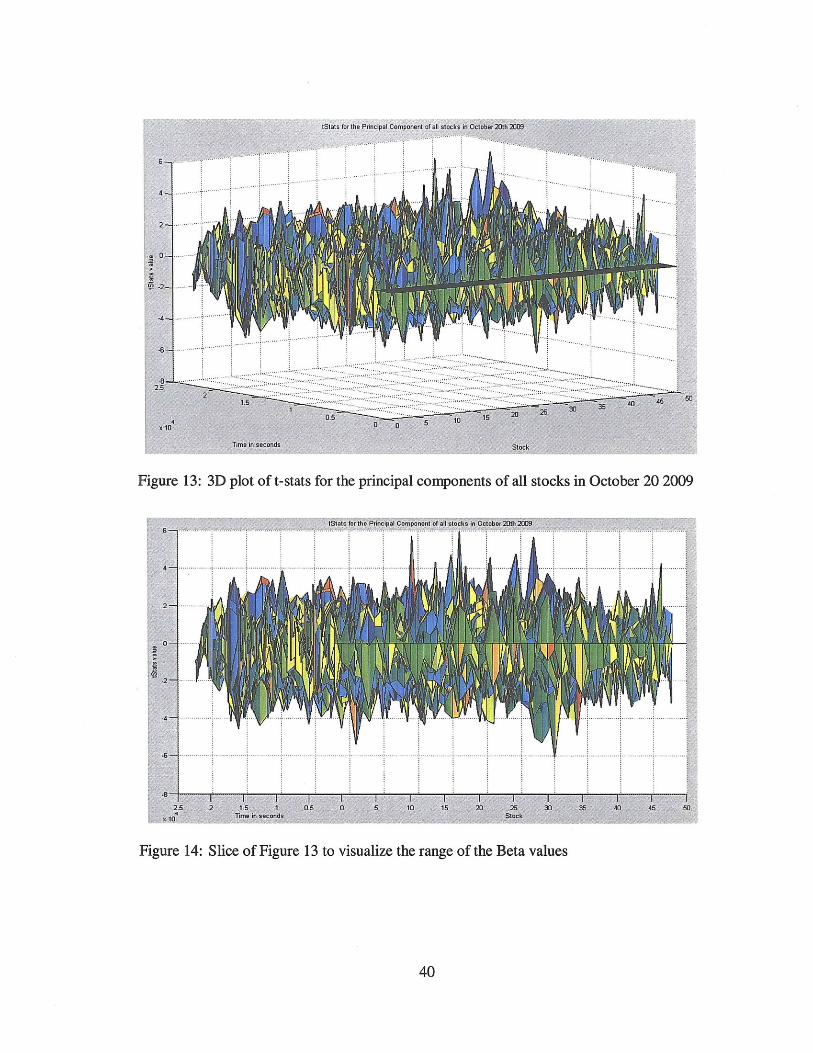
Figure 13: 3D plot of t-stats for the principal components of all stocks in October 20 2009

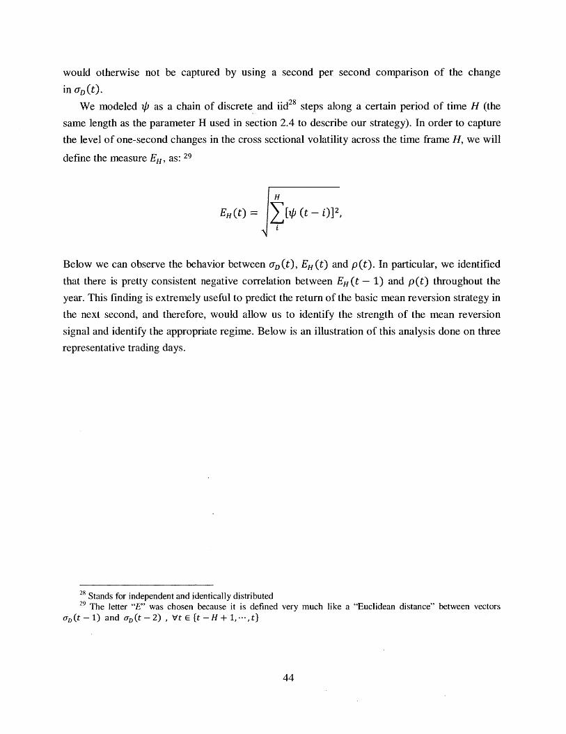
Figure 14: Slice of Figure 13 to visualize the range of the Beta values

3 Regime Switching Model

3.1 Description of the Model

From the results obtained in the first model we arrived to two possible conclusions:

(i) The expected returns we determined by our prediction model were not representative of the

market's behavior.

(ii) The expected returns were representative of the market's behavior, but only at certain times

and under certain conditions. The market could change behavior when certain conditions are

met. Knowing the fair value of a stock is not a sufficient reason for the market to trade

accordingly.

As we strongly believe in all the reasons that back our estimation of future returns, we will show

evidence that our second conclusion is correct. We will demonstrate what happens if we predict

when the market changes behavior and change our trading strategy accordingly. More

specifically we believe that there are two main regimes in which the market works: one regime is

"mean-reversion" , and the other regime is "momentum" . This assumption would explain

why we have to change our trading strategy from mean-reversion" to "momentum" when the25market conditions change in order to generate significant alpha.

Our expected "momentum" behavior in the high frequency environment is motivated by

many of the concepts developed by those who question the rational and efficient behavior in the

traditional low frequency arena. Yes, we refute the "Efficient Market Hypothesis" and strongly

believe in the "Adaptive Market Hypothesis" instead. Moreover, we believe that the latter

perfectly applies to the high frequency world 26 . There are no better words to describe these

thoughts as those used by Lo and Mueller in their 2010 paper:

"This perspective suggests an alternative to the antiseptic world of rational expectations and

efficient markets, one in which market forces and preferences interact to yield a much more

dynamic economy driven by competition, natural selection, and the diversity of individual and

institutional behavior. This approach to financial markets, which we refer to as the "Adaptive

Markets Hypothesis" (Farmer and Lo, 1999; Farmer, 2002; Lo, 2004, 2005; and Brennan and Lo,

25 This means that in a "mean-reversion" regime we expect the real returns to converge to the theoretical

returns, and in a "momentum" regime we expect real returns to further diverge from the theoretical returns.26 Based on all the examples we gave on how "ultra high frequency" players make their decisions, it seems

closer to playing a poker game, than to solving a valuation problem. Therefore, irrationality in trading, as seen fromthe "classic" point of view, could be very common in this arena.

2009), is a far cry from theoretical physics, and calls for a more sophisticated view of the rolethat uncertainty plays in quantitative models of economics and finance."

In addition we also want to recall the harmonic oscillator problem used as an example of a"Level 4 Risk" problem in Lo-Mueller 2010. As mentioned before, the type of risk we deal within finance problems is usually characterized by this level of risk. The problem used as "Level 4Risk" example was a "Regime Switching" harmonic oscillator of the following characteristics:

xWt = I Wt X1(t) + (1 - 1(t)) Xz2t)

xi(t) = Ai cos(wit + <i) , i = 1,2

"...where the binary indicator I(t) determines which of the two oscillators x1 (t) or x 2 (t) isgenerating the observed process x(t), and let I(t) be a simple two-state Markov process withthe following simple transition probability matrix P:"

I(t) = 1 I(t) = 0

_ IW - 1) =1 (1 - p pI(t- 1) 0 p 1 -p)

Given all these ideas, our challenge is now to look for a regime switching signal. Beingconsistent with our thoughts, we believe that the principal components are the best representationof the main risk in the universe under study, and it is also from them that we will obtain thesignal to indicate if the market is in the "mean-reversion" or in the "momentum" regime.

Our first basic underlying and very intuitive idea is to expect the momentum regime to berelated to the sprouting of dislocations in the market. One example of this type of behavior isgiven by all the dislocations in the financial crises (widening of "on the run" vs. "off the run"bond spreads in the LTCM crisis, all sorts of irrational credit spreads in the Credit Crunch in2009 , etc.) where momentum strategies happen to be very successful.

In particular, we will look at dislocations in the main components of risk, which are indeedthe principal components. To identify these dislocations we created a variable that we called the"Cross Sectional Volatility of the Principal Components", which is nothing more than thestandard deviation of the stock returns projected on the selected eigenvectors obtained from thePCA at a certain point in time. This Cross Sectional Volatility, oD(t),could be explained asfollows:

k 2

JD(t) = j(d - , Vt E t1,2, --- , T}k - 1j=1

where D is the time series of the "dimensionally reduced returns" mentioned in section 2.4, and

k is the number of eigenvectors chosen to obtain the dimensionally reduced returns, dt; is the

"dimensionally reduced return" j (out of the k defining our reduced-space) at time t. dt is

the cross sectional mean at time t defined as:

k

j=1

On our following analysis we identified the following behavior. As the short term changes in oD

appeared to be more pronounced - identified by very narrow peaks in the aD time series -

cumulative returns from the basic mean-reversion strategy seemed to decrease. One better way of

looking into this behavior is rather looking at the "changes" in uD over time, rather than the

value itself. Let's define V) as:

dqD

dt

27where ip is the continuous time form of the change in aD in time

We define the time series of cumulative returns of the basic strategy as:

p = p(t),

We want to somehow include the intuition we learned on the graphs we show below, and capture

"short term" aD (t) changes (or "peaks"), and measure the aggregate value of these changes over

a period of time. We believe that this framework should create clearer "momentum" signals that

27 We will keep the continuous time forms to better illustrate the concepts, although all the problems are beingsolved in discrete time, using the discrete time series of returns obtained from our dataset.

would otherwise not be captured by using a second per second comparison of the change

in oD-(t).

We modeled V) as a chain of discrete and iid28 steps along a certain period of time H (the

same length as the parameter H used in section 2.4 to describe our strategy). In order to capture

the level of one-second changes in the cross sectional volatility across the time frame H, we will

define the measure EH, as: 29

H

EH(t) = [ (t - i)] 2,

Below we can observe the behavior between 0 D(t), EH(t) and p(t). In particular, we identified

that there is pretty consistent negative correlation between EH (t - 1) and p(t) throughout the

year. This finding is extremely useful to predict the return of the basic mean reversion strategy in

the next second, and therefore, would allow us to identify the strength of the mean reversion

signal and identify the appropriate regime. Below is an illustration of this analysis done on three

representative trading days.

28 Stands for independent and identically distributed29 The letter "E' was chosen because it is defined very much like a "Euclidean distance" between vectors

o-D(t -1) and o-(t - 2) , Vt E {t - H + 1,---, t}

__- 1_1_ __11_- - -- .1 ,--A4,i NWF-!-Fi, .,w4 -- -,-i-.. - I I -___ -__-1-._1__1.___ ONOWO I I , -- _,---____- 0 - _- - -.- _ ________

February 10 2009:

0.45%

0.36%

0.27%

0.18% -

0.09% -

0.00%

1.30%

0.67%

0.03%

-0.60%

-1.23%

-1.87%

--- - I- -L ------ ----------- -- ------ ----- --

III 16.110 11 1 1 . 11 -

- - - -1

- - - - - - --

L -, ---- --- --- --- --= =- -- -- =

-2.50% -9:30 10:35 11:40 12:45 13:50 14:55 16:00

Figure 15: The top plot shows the cross sectional volatility of the dimensionally reduced time

series, aD (t) over the course of the day. The bottom plot shows the cumulative returns p(t),

over the course of the day.

T T -- I

- - -- - - - - - - - - - - - - - - - -

0.013

0.011

0.009

0.006

0.004

* ~ 0.002 -- - - - -- - - - - - - -I-- - - - - - - - -

0.000 , ,

9:30 10:35 11:40 12:45 13:50 14:55 16:00

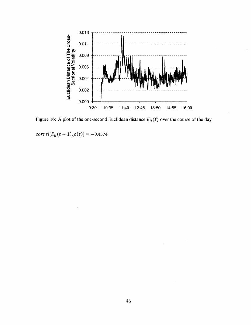
Figure 16: A plot of the one-second Euclidean distance EH (t) over the course of the day

correl[EH(t - 1),p(t)] = -0.4574

July 20 2009:

>, 0.10% - - - - - - -- - - - - --- - -0

-0 0 % -- --- - - - - - -- --- - -

C0

-0.10% --Cl)

(0

.)0.05%

0.00%

0.00% - rTC

0.40% - - - - - - - - - - - - -- - - -(D

9:30 10:35 11:40 12:45 13:50 14:55 16:00

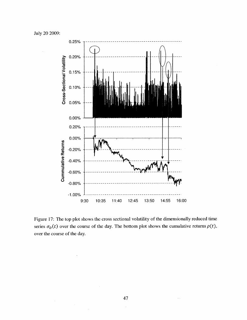
Figure 17: The top plot shows the cross sectional volatility of the dimensionally reduced time

series o-D (t) over the course of the day. The bottom plot shows the cumulative returns p(t),

over the course of the day.

(0

I.

(D) 0

0>

*~C

wo

Ca

0.006

0.005

0.004

0.003

0.002

0.001

0.0009:30 10:35 11:40 12:45 13:50 14:55 16:00

Figure 18: A plot of the one-second Euclidean distance EH (t) over the course of the day

correl[EH(t - 1),p(t)] = -0.2150

December 3 2009:

0.18%

(U)0

C,)

E)Eo

0.15 0X

0.12X

0.090/

0.060X

0.030X

0.000/c

0.300/c

0. 20/c

0. 10 /C

0. 00/C

-0. 10 /C

-0. 200%c

-0.30%

-0.40%

-0.50%A

Figure 19: The top plot shows the cross sectional volatility of the dimensionally reduced time

series oD(t) over the course of the day. The bottom plot shows the cumulative returns p(t),

over the course of the day.

- - - ---- ----------------------- ---- -

9:30 10:35 11:40 12:45 13:50 14:55 16:00

---------------------------------------------- -

---------- -------------- - ----------- -A- - j -- --- ------ ---------- - -------------

I ,

-- -- -- -- --- - -- - ---- ----- -- --

0.004 ------------------------------------- ---------

0.003 - ------- ---------- -- --

0 oc o

0

-a 0.001 -

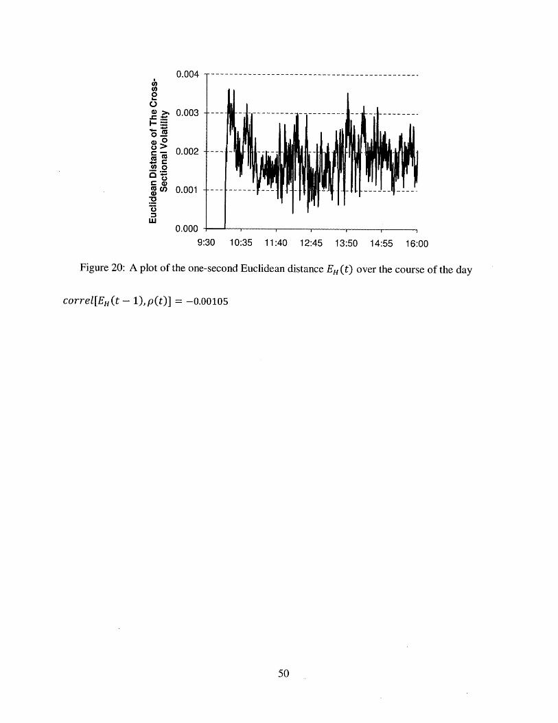
00C0.001 ---- ----- --------

9:30 10:35 11:40 12:45 13:50 14:55 16:00

Figure 20: A plot of the one-second Euclidean distance EH(t) over the course of the day

correl[EC(t - 1),p(t)] = -0.00105

This finding is extremely consistent with our basic intuition: The sprouting of principal

components dislocations at time t induces negative returns on a mean reversion strategy at t+l, or

in better words, the sprouting of principal components triggers momentum.

We now only have to model these discrete changes in the dislocations of principal

components, capture some order of magnitude of these changes in a period of time of our

interest, and build a "regime switching" signal. This signal would tell us to either agree with

basic mean-reversion signal and trade according to our base strategy, or refute this signal

because of evidence of "momentum", and trade opposite of our base strategy.

The regime switching strategy would then follow:

EH(t)- EH(t - 1)

at time t. If this value happens to be greater than zero, we understand that the "aggregate value of

principal components dislocation" seems to be increasing and we should therefore, trade on

"momentum". If this happens to be equal or lower than zero, then we stick to the mean-reversion

signal of the basic model. As we can see, "momentum" seems to be linked to the "acceleration"

of oD (the cross sectional volatility of principal components). This is totally intuitive to us. On

the next section we will show an analysis of the results of the combined regime switching

strategy.

3.2 Regime Switching Model Results

After applying the "Regime Switching" signal to our basic mean reversion strategy we improved

the results significantly:

Cumulative Log Returns

80% -----------------------------------------------------

70% ----------

60%

50%

40% -- ------------

30% --

20%

10% ~~-- ------ - - - - - - - - - - - - - - - - - - - - -

0%Jan Mar May Jul Sep Oct Dec

Figure 21: The plot of the accumulated log returns over a period of 251 trading days in 2009

Mean Volatility Sharpe Ratio Max Drawdown76.93% 10.03% 7.67 -1.45%

Table 9: Statistics of the strategy's performance across the entire year of 2009

4 Potential Improvements

Because of the scope of our problem we did not have time to investigate certain issues that could

affect our alpha model. However, below are several suggestions for improving the model.

4.1 Clustering

One such issue is the scaling to thousands of stocks vs. the universe of 50 stocks that we

investigated. Assuming that our chosen stock universe is representative of a much larger universe

of stocks could seem a bit questionable. For instance, when looking at a broader range of stocks

we will run into fewer liquid stocks and one can argue that this would affect the sparsity of the

variance-covariance matrix which in turn would give us a very different principal component

analysis. In order to tackle this problem we can cluster the stocks into smaller buckets, each

characterized by their principal components.

For example, if we have 1000 stocks that we want to divide into 10 buckets of 100 stocks

each, we can simply run a PCA on the entire universe. We then regress each stock's return with

the first principal component. The 100 stocks that show the highest beta will be placed in one

bucket. We then subtract the first component from the stock returns and do a PCA on the

residual. We repeat the process for the next highest principal component. This is done until all

stocks are placed in a certain bucket. Although there may be an overlap between buckets, it can

easily be resolved by comparing the size of the beta of the stock that shows up in more than one

bucket and placing it in the bucket in which it has the highest correlation to the bucket's

principal component (highest beta). One problem with this method is that the last clusters will be

defined by using lower eigenvalue principal components, and therefore bucketed by using very

"noisy" eigenvectors.

Another idea for clustering, especially for those who want to preserve universe wide PCA

characteristics across every cluster and at the same time reduce the "noisy" eigenvector effect

mentioned before, is to simply do a naive random clustering. This method will preserve the

universe wide PCA characteristics in every cluster if we keep the same eigenvectors for every

cluster. We can do this by taking the mean of all the eigenvectors of the same hierarchy across

every cluster. However, this would bring a different eigenvector noise, given that each of them

would no longer represent exactly its corresponding principal component in the cluster. This

seems trivial and unsophisticated, but may make help keep a similar PCA for every cluster.

Notice that the 1000 stocks that we had earlier, will be now divided into 10 buckets of 100 stocks

each. Now doing a PCA on the smaller universes would be 100 times faster for each bucket

compared to the universe wide PCA. This is because the variance-covariance matrix is smaller

by a factor 10 both in the row and in the column dimensions. Doing so for all 10 buckets will

give us a unified PCA but 10 times faster.

4.2 Selection of Eigenvectors

One of the things that could be done better to increase predictive power in the model is work on

the criterion to select the number of eigenvectors (or principal components) to use after the PCA.

As you may recall, these selected eigenvectors construct the feature matrix that transforms our

original time series to a reduced-space of returns. These reduced-space returns ultimately build

the explanatory time series of variables to use in the linear model to predict cumulative future

returns.

We suggest the use of a simple autoregressive model on the time series of the number of

eigenvectors that maximize the Sharpe Ratio at each trading period. The approach should consist

on the following steps:

(i) Compute an optimization of the number or eigenvectors used vs. the Sharpe Ratio ex-post, at

the end of each trading period

(ii) Record this optimum number of eigenvectors on a vector (let's call this number of

eigenvectors, or principal components: et)

(iii)We should allow for a reasonable time to pass in order to provide robustness to the time

series which expresses the optimum number of eigenvectors at each time (we suggest one

third of the trading day.) We can predict these optimum number of eigenvectors to be used in

our main predictive model, by using the past returns of the model on that day as a validation

dataset. The suggested way to compute this is by building an AR model of the following

characteristics:

et = #1 et-I + f 2 et- 2 + f 3 et- 3 -- + fp et-p + 7t,p , -qt,p ~ N (0, U2)

where et-p is the number of eigenvectors at time period (t - p) that would have generated

the maximum Sharpe Ratio, and et is the predicted optimum number of eigenvectors to use at

time (t) to build our trading signal. 30 The errors are assumed normally distributed with

constant variance.

In addition, we suggest the use of a Maximum Likelihood Estimation function31 and the Akaike

or Bayesian Information criterions (AIC or BIC) to pick the optimum number of autoregressive

steps in the AR model. The criterions introduce a penalty for each increment in the number of

autoregressive steps to a log likelihood function used to determine p*, which is defined as the

optimum number of autoregressive steps p. The problem to solve for p* should be approached as

follows:

(i) Start by specifying the maximum possible order P. Make sure that P grows with the sample

size but not too fast:

lim p=oo, lim -= 0T-om T-4oT

(ii) Define,2

p* = arg max - L (0; p) - penatly (p)0:sp:s p T

where the penalty p is as follows:2

penatly (p) with AIC criterion =- p NzT

In T 2penatly (p) with BIC criterion = p NzT

and T is the number of values in the time series to autoregress.

L (0; p) is the following log likelihood function with vector of parameters 0 = o2 and

p number of autoregressive steps:

30 The optimum value at each period can be easily computed at each step, and recorded in a vector to be usedlater, by a simple iteration that computes the Sharpe Ratio of the trading model for each number of possibleeigenvalues.

31 Most of the concepts in sections 4.2 and 4.3 have been obtained from Leonid Kogan's lectures on "Analyticsof Finance" in the MIT Sloan School of Management.

L 6)= T=-1 - n41o2 (et-fl1 et- a- f2 et-2 - fl3 et-s ...- flp et-p)z

We should be aware that in larger samples BIC selects a lower number than AIC.

4.3 NLS

Another suggested improvement for the predictive model of cumulative returns, would be to

make it a little bit more sophisticated and allow for a function to compute weighted lagging

observations of the principal component time series of returns, or as previously called, the

dimensionally reduced time series of returns.

We recall the basic model we suggested:

H

rt+1 + + rt+H = fI1 Dt-i,1i=0

We now introduce a "Beta Function" of the type:

bH,k0, 0) = ,

H

rt+1 + + rt+H = f 1 H b, 1 (i, 0) Di,1i=0

H

+ '' k Dti,k +llt+H,H

i=0

f (X, A,0 -- X" ( - X)

H

+ -- + Y bH,k (i, 0) Dti,k + ?7t+H,Hi=o

The introduction of this function that will perform optimum weighting of principal components

will introduce much more flexibility and accuracy to the model, but this will no longer be an

OLS problem; this will be an NLS type of problem.33

32 This is nothing more than the original time series of returns projected over the feature vector of choseneigenvectors after the PCA.

3 Consistent with the risk levels defined in Mueller and Lo's paper mentioned before, this would be fitting aproblem still assuming the 3rd Level of risk (Fully Reducible Uncertainty), and in our view to the most complex ofits boundaries where non-trivial challenges such as non-linear parameter estimation arise.

4.4 Other

The challenge of the two suggestions is the intensity of the computer power needed to solve the

models on a dynamic high frequency strategy. As final suggestions we want to recommend the

following numerical methods to solve some of the problems presented in this paper:

(i) To compute the PCA we suggest not getting into covariance matrix computations. Instead we

suggest a Singular Value Decomposition (SVD) approach of the type:

M= UZVT

where the columns of VT are the eigenvectors of MT * M , the columns of U are the

eigenvectors of M * MT , and the diagonal terms in Y are the square roots of the eigenvalues

of MT * M

The matrices containing eigenvalues and eigenvectors can be computed much more

efficiently and quickly using numerical methods such as the Jacobi algorithm, that would

save a tremendous amount of time in computer driven algorithms.

(ii) Our other suggestion is to solve the NLS problem when including the weighting functions on

the model of principal components to predict future cumulative returns, also by using

numerical methods such as the Marquardt Levenberg algorithm, which is probably the

convergence algorithm that provides a better tradeoff between the complexity to implement

and code and the quality and computation time.

(iii)Lastly, we suggest trying the use of GPU (graphing processing units) as sources to enhance

computing speed as the problem gets more computationally intense and databases get larger.

As certain GPUs have hundreds of cores in them, it is possible to divide the mathematical

complex problem into hundreds of smaller problems that will be done in parallel. This can

dramatically reduce the latency of certain computations such as calculating the variance-

covariance matrix of a very large universe of stocks.

5 Conclusion

In conclusion, we achieved our initial objective of presenting evidence that there are significant

opportunities to generate alpha in the high frequency environment in the US equity markets. In

particular, we found sources of potential alpha in the arena characterized by holding periods

between what we called the typical "ultra high frequency" 34 environment and traditional

statistical arbitrage environment.

We achieved our goal by building a model that:

(i) Determined short term equity valuation by predicting cumulative returns based on the

cumulative sum of principal components.

(ii) Identified regimes by analyzing the aggregate change in the dislocations of these principal

components, measured by computing their cross sectional volatility.

Although there are many assumptions that in reality may erode our estimated alpha due to real

transaction costs 35, the fact that we used very liquid equities in our model, should mitigate this

potential erosion. We do not suggest that it may not happen, we simply believe that a Sharpe

Ratio of 7, considering the universe of liquid stocks that we used, is strong enough evidence to

suggest that there are significant opportunities to generate excess returns in our environment. In

addition, we also provided evidence that the "Fundamental Law of Active Management" works

well. We can see in section 2.6 that the summary statistics of the cumulative-return predictions

made on a given day are quite weak from a statistical significance perspective. Nevertheless, this

lack of precision did not prevent us from obtaining significant theoretical alpha in our model.

Overall, we believe that the high frequency environment offers a wide range of opportunities

to generate alpha; even more, if we consider how we can benefit from the "Fundamental Law of

Active Management". We believe that we provided strong evidence to support this hypothesis by

presenting a plausible trading strategy as an example.

3 See definition in section 1.1, footnote #3.35 We assume that trades were executed at mid market prices, and that we can execute a trade based on the last

mid-price within the same second we recognized the trade. See simplifying assumptions in section 2.5

References

Mueller M. and A. Lo, 2010, "WARNING: Physics Envy May Be Hazardous To Your Wealth!",

MIT Sloan School of Management; National Bureau of Economic Research (NBER);

Massachusetts Institute of Technology, Center for Theoretical Physics.

Grinold R. and Kahn R., "Active Portfolio Management: A Quantitative Approach for Producing

Superior Returns and Controlling Risk", Mc Graw Hill, second edition.

Jurek J. and Yang H., 2007, "Dynamic Portfolio Selection in Arbitrage", Bendheim Center for

Finance, Princeton University.

Khandani, A. and A. Lo, 2007, "What Happened to the Quants in August 2007?", Journal of

Investment Management 5, 5-54.

Lo A. and C. MacKinlay, 1990a, "When Are Contrarian Profits Due to Stock Market

Overreaction?," Review of Financial Studies 3, 175-206.

Lo, A., 2004, "The Adaptive Markets Hypothesis: Market Efficiency from an Evolutionary

Perspective", Journal of Portfolio Management 30, 15-29.

Avellaneda M. and J.H. Lee, 2009, "Statistical Arbitrage in the US Equities Market", Courant

Institute of Mathematical Sciences (NYU), Finance Concepts, Paris, France.

Campbell, Lo, and MacKinlay, 1997, "The Econometrics of Financial Markets",

Princeton University Press.