developing a mode choice model for small and medium … · developing a mode choice model for small...

Technical Report Documentation . Report No.

FHWA/TX-14/0-6766-1

2. Government Accession No.

3. Recipient’s Catalog No.

4. Title and Subtitle

Developing a Mode Choice Model for Small and Medium MPOs

5. Report Date

February 2014; Published September 2014

6. Performing Organization Code 7. Author(s)

Dubey, S., Deng, J., Hoklas, M, Castrol, M., Loftus-Otway, L., and Bhat, C.

8. Performing Organization Report No.

0-6766-1

9. Performing Organization Name and Address

Center for Transportation Research The University of Texas at Austin 1616 Guadalupe Street, Suite 4.202 Austin, TX 78701

10. Work Unit No. (TRAIS) 11. Contract or Grant No.

0-6766

12. Sponsoring Agency Name and Address

Texas Department of Transportation Research and Technology Implementation Office P.O. Box 5080 Austin, TX 78763-5080

13. Type of Report and Period Covered

Technical Report

November 2012–December 2013

14. Sponsoring Agency Code

15. Supplementary Notes Project performed in cooperation with the Texas Department of Transportation and the Federal Highway Administration.

16. Abstract

This project developed a process and framework for generating the inputs needed for estimating a travel mode choice model that includes the transit mode, and developing a framework for implementing the results of an estimated travel mode choice model to project mode shares in response to demographic changes and improvements in transit service. In generating inputs for estimating a mode choice model, an important component is network skims (travel times and costs) by alternative modes. Most metropolitan planning organizations (MPOs) have good geographic information systems (GIS)-based representations of the highway network, which can be used to generate drive-alone and shared-ride skims. However, this is not the case with transit skims due to the lack of a good GIS-based representation of the transit network, especially for bus stops. The project manually geo-coded bus stop information onto the highway network, and used assumptions to generate transit paths and corresponding zone-to-zone transit skims. A guidebook provides a step-by-step procedure for developing skims. The database for estimation was developed using household survey data (2004) on trip characteristics. Two demographic variables were used in the mode choice model: household size and income. The models have been embedded into a software forecasting platform to predict modal share shifts between each pair of TAZs (and the region as a whole) due to changes in income levels and/or household size over time. The models can also be used to assess the impacts of transit improvements for in-vehicle and out-of-vehicle transit times. Further data collection from transit surveys is recommended to enhance the model’s capacity to estimate the time and cost effects based on preferences. A georeferenced coordinate system for bus stop locations would also improve the transit skim generation process.

17. Key Words

Mode Choice Model, Network Skims, Metropolitan Planning Organizations, Urban Travel Demand, Trip Generation, Trip Distribution, Texas Package Suite, Transportation Demand Model.

18. Distribution Statement

No restrictions. This document is available to the public through the National Technical Information Service, Springfield, Virginia 22161; www.ntis.gov.

19. Security Classif. (of report) Unclassified

20. Security Classif. (of this page) Unclassified

21. No. of pages 134

22. Price

Form DOT F 1700.7 (8-72) Reproduction of completed page authorized

Developing a Model Choice Model for Small and Medium MPOs Subodh Dubey Jun Deng Megan Marie Hoklas Marisol Castrol Lisa Loftus-Otway Chandra Bhat

CTR Technical Report: 0-6766-1 Report Date: February 2014 Project: 0-6766 Project Title: A Generic Mode Choice Model Applicable for Small and Medium-Sized

MPOs Sponsoring Agency: Texas Department of Transportation Performing Agency: Center for Transportation Research at The University of Texas at Austin Project performed in cooperation with the Texas Department of Transportation and the Federal Highway Administration.

Center for Transportation Research The University of Texas at Austin 1616 Guadalupe, Suite 4.202 Austin, TX 78701 http://ctr.utexas.edu/

v

Disclaimers Author's Disclaimer: The contents of this report reflect the views of the authors, who

are responsible for the facts and the accuracy of the data presented herein. The contents do not necessarily reflect the official view or policies of the Federal Highway Administration or the Texas Department of Transportation (TxDOT). This report does not constitute a standard, specification, or regulation.

Patent Disclaimer: There was no invention or discovery conceived or first actually reduced to practice in the course of or under this contract, including any art, method, process, machine manufacture, design or composition of matter, or any new useful improvement thereof, or any variety of plant, which is or may be patentable under the patent laws of the United States of America or any foreign country.

Engineering Disclaimer NOT INTENDED FOR CONSTRUCTION, BIDDING, OR PERMIT PURPOSES.

Project Engineer: Dr. Chandra Bhat

Professional Engineer License State and Number: Texas No. 88971 P. E. Designation: Research Supervisor

vi

Acknowledgments The authors wish to thank Wade Odell, RTI, Research Project Manager; James Burnett,

Transportation Program and Planning (TPP) Project Advisor; Gabriel Contreras, TPP, Project Advisor; Greg Lancaster, TPP, Project Advisor; George Petrek, TPP, Project Advisor; Mike Schofield, TPP, Project Advisor; and Janie Temple, TPP, Project Advisor.

Products Appendix B contains 0-6766-P1, Forecasting Tool User Manual, also available as a

stand-alone document.

Accompanying CD The accompanying CD contains the Excel-based forecasting tool and the Forecasting

Tool User Manual. Also included are a MATLAB script and input files for testing purposes. This script is discussed at the end of Appendix A.

• Stop_TAZ_Code.m = MATLAB script file • LUBBOCK_TAZ_XY.csv = input file for TAZ number and coordinates • LUBBOCK_Stops.csv = input file for Stop number and coordinates

vii

Table of Contents

Chapter 1. Introduction.................................................................................................................1 1.1 Background ............................................................................................................................1 1.2 Objective of Research Project ................................................................................................2

Chapter 2. Literature Review .......................................................................................................5 2.1 Mode Choice Models .............................................................................................................5

2.1.1 Overview .........................................................................................................................5 2.2 Mode Choice Models Outside of Texas ................................................................................7 2.3 Mode Choice Models in Texas ............................................................................................11

2.3.1 Capital Metro MPO (CAMPO) .....................................................................................12 2.3.2 Houston-Galveston Area Council (HGAC) ..................................................................13 2.3.3 San Antonio-Bexar County MPO (SABCMPO) ..........................................................15 2.3.4 North Central Texas Council of Governments (NCTCOG) .........................................16

Chapter 3. Incorporating a Mode Choice Component for Small and Medium-Sized MPOs in Texas .............................................................................................................................19

3.1.1 Population Growth ........................................................................................................19 3.1.2 Mode Choice Shares .....................................................................................................20 3.1.3 Strategic Planning Goals ...............................................................................................22

3.2 Recommendations ................................................................................................................25

Chapter 4. Develop a Forecasting Approach and Model Design.............................................29 4.1 The Texas Package ..............................................................................................................29 4.2 Mode Choice Model Recommendations ..............................................................................30 4.3 Model Specification .............................................................................................................31 4.4 Forecasting Approach ..........................................................................................................33 4.5 Next Steps ............................................................................................................................33

Chapter 5. Procedure to Develop Skims ....................................................................................35 5.1 Skim Components ................................................................................................................35 5.2 Mode Availability ................................................................................................................37 5.3 Skim Development ..............................................................................................................37

5.3.1 Drive Alone and Car Sharing ........................................................................................37 5.3.2 Transit ...........................................................................................................................39 5.3.3 Walk and Bicycle ..........................................................................................................40

5.4 Summary and Next Steps .....................................................................................................40

Chapter 6. Transit Skim Generation for Texas MPOs ............................................................41 6.1 Selected MPOs .....................................................................................................................41 6.2 Transit Characteristics .........................................................................................................41

6.2.1 Bryan-College Station MPO .........................................................................................41 6.2.2 San Angelo MPO ..........................................................................................................42 6.2.3 Longview MPO .............................................................................................................43 6.2.4 Lubbock MPO ...............................................................................................................44

6.3 Transit Skim Generation ......................................................................................................45 6.4 Summary and Next Steps .....................................................................................................46

viii

Chapter 7. Procedure to Prepare Data ......................................................................................47 7.1 Procedure for Survey Data Extraction .................................................................................48 7.2 Skim Generation ..................................................................................................................50

7.2.1 Skim Generation for Drive Alone Mode.......................................................................50 7.2.2 Skim Generation for Carpool Mode .............................................................................51 7.2.3 Skim Generation for Transit Mode ...............................................................................52 7.2.4 Skim Generation for Walk Mode ..................................................................................53 7.2.5 Skim Generation for Bike Mode ...................................................................................53

7.3 Summary and Next Steps .....................................................................................................53

Chapter 8. Model Development ..................................................................................................55 8.1 Introduction and Overview ..................................................................................................55 8.2 Lubbock MPO ......................................................................................................................55

8.2.1 Traffic Analysis Zones ..................................................................................................55 8.2.2 Modes ............................................................................................................................55 8.2.3 Network and Level-of-Service Preparation ..................................................................55 8.2.4 Explanatory Variables ...................................................................................................56 8.2.5 Data ...............................................................................................................................56

8.3 Longview MPO ....................................................................................................................59 8.3.1 Traffic Analysis Zone ...................................................................................................59 8.3.2 Modes ............................................................................................................................59 8.3.3 Network and Level-of-Service Preparation ..................................................................59 8.3.4 Explanatory Variables ...................................................................................................60 8.3.5 Data ...............................................................................................................................60

Chapter 9. Conclusions ................................................................................................................63

References .....................................................................................................................................65

Appendix A. Guide to Model Skim Generation Development in TransCAD and ArcMap 10.1 .................................................................................................................................69

Appendix B. Forecasting Tool User Manual ...........................................................................107

Appendix C. The Multinomial Logit (MNL) Model ...............................................................117

Appendix D. The Nested Logit (NL) Model.............................................................................119

Appendix E. Travel Demand Models of MPOs Outside of Texas .........................................121

ix

List of Figures Figure 1.1: Four-step trip-based approach ...................................................................................... 1 Figure 1.2: Texas MPOs with a travel mode choice component in their TDM .............................. 3 Figure 2.1: NL model structure of GCMPC’s mode choice model .............................................. 10 Figure 2.2: NL model structure of AMBAG’s mode choice model ............................................. 11 Figure 2.3: NL model structure of CAMPO’s mode choice model .............................................. 14 Figure 2.4: NL model structure of H-CAG’s mode choice model ............................................... 14 Figure 2.5: NL model structure of SABCMPO’s mode choice model ......................................... 16 Figure 2.6: NL model structure of NCTCOG’s mode choice model ............................................ 18 Figure 4.1: Texas Package inputs ................................................................................................. 29 Figure 6.1: The selected Texas MPOs .......................................................................................... 41 Figure 7.1: Selected study area ..................................................................................................... 47 Figure A.1: File selection menu .................................................................................................... 70 Figure A.2: Import shapefile window ........................................................................................... 70 Figure A.3: File save menu ........................................................................................................... 71 Figure A.4: Geographic file selection window ............................................................................. 71 Figure A.5: TAZ visual setting window ....................................................................................... 72 Figure A.6: Layer addition window .............................................................................................. 72 Figure A.7: Layer visualization window ...................................................................................... 73 Figure A.8: Layer visualization window ...................................................................................... 73 Figure A.9: Toolbar ...................................................................................................................... 74 Figure A.10: Visual adjustment window for layers ...................................................................... 74 Figure A.11: Tools ribbon............................................................................................................. 75 Figure A.12: Selection window .................................................................................................... 76 Figure A.13: Viewing the centroid set .......................................................................................... 76 Figure A.14: Binary network creation window ............................................................................ 77 Figure A.15: Status bar ................................................................................................................. 77 Figure A.16: Multiple shortest path menu .................................................................................... 78 Figure A.17: Additional skim selection window .......................................................................... 78 Figure A.18: Toolbar .................................................................................................................... 79 Figure A.19: Matrix export window ............................................................................................. 79 Figure A.20: Network setting window.......................................................................................... 80 Figure A.21:Network update window ........................................................................................... 81 Figure A.22: Condition window ................................................................................................... 81 Figure A.23: Network info window .............................................................................................. 82 Figure A.24: Re-enable all the links ............................................................................................. 82 Figure A.25: Input files in the workspace ..................................................................................... 83 Figure A.26: Georeferencing toolbar ............................................................................................ 84

x

Figure A.27: Shift tool .................................................................................................................. 84 Figure A.28: Images after using shift tool .................................................................................... 85 Figure A.29: Link table button ...................................................................................................... 85 Figure A.30: Link Table ............................................................................................................... 85 Figure A.31: Add control point button ......................................................................................... 86 Figure A.32:Adding control points ............................................................................................... 86 Figure A.33: RMSE value............................................................................................................. 86 Figure A.34: Rectify option under georeferencing toolbar ........................................................... 87 Figure A.35: Saving the image ..................................................................................................... 87 Figure A.36: ArcCatalog window ................................................................................................. 88 Figure A.37: Adding shapefile to the working folder ................................................................... 89 Figure A.38: Shapefile property box ............................................................................................ 90 Figure A.39: Coordinate system window ..................................................................................... 90 Figure A.40: Creating feature dataset ........................................................................................... 92 Figure A.41: Feature class definition ............................................................................................ 93 Figure A.42: Shapefiles in table of contents window ................................................................... 94 Figure A.43: Start editing option box ........................................................................................... 94 Figure A.44: Create feature window ............................................................................................. 95 Figure A.45: Point option on Editor Toolbar ................................................................................ 95 Figure A.46: Save edits and stop editing options ......................................................................... 96 Figure A.47: Attribute table for bus stops .................................................................................... 96 Figure A.48: Add field option to table .......................................................................................... 97 Figure A.49: Defining field name and type .................................................................................. 97 Figure A.50: Calculate X coordinates ........................................................................................... 98 Figure A.51: Calculate Y coordinates ........................................................................................... 99 Figure A.52: Snapping toolbar ...................................................................................................... 99 Figure A.53: Snapping toolbar options ....................................................................................... 100 Figure A.54: New snapping tolerance setting window ............................................................... 100 Figure A.55: Classic snapping option window ........................................................................... 101 Figure A.56: Classic snapping tolerance setting window ........................................................... 102 Figure A.57: Create feature window (line option) ...................................................................... 102 Figure A.58: Line option on Editor Toolbar ............................................................................... 102 Figure A.59: Final_bus_links shapefile ...................................................................................... 103 Figure A.60: Data export window .............................................................................................. 103 Figure A.61: Output feature class window ................................................................................. 104 Figure B.1: Forecasting Tool Input Sheet ................................................................................... 108 Figure B.2: Empty Cell Message ................................................................................................ 112 Figure B.3: Empty Colored Cell ................................................................................................. 113 Figure B.4: Delete the Old Sheets............................................................................................... 115 Figure C.1: Mode choice framework of MNL models ............................................................... 117 Figure D.1: Mode choice framework of NL models ................................................................... 119

xi

List of Tables Table 1.1: Population-based classification of Texas MPOs ........................................................... 4 Table 2.1: Common variables used in travel mode choice models ................................................. 6 Table 2.2: TDMs of MPOs outside of Texas .................................................................................. 8 Table 2.3: Mode choice models of MPOs outside of Texas ........................................................... 9 Table 2.5: List of explanatory variables in NCTCOG mode choice model .................................. 17 Table 3.1: MPO population growth .............................................................................................. 20 Table 3.2: Mode shares for HB work trips ................................................................................... 21 Table 3.3: Strategic planning goals related to mode choices ........................................................ 23 Table 3.4: Recommendation on incorporating a mode choice model in the TDM ....................... 26 Table 4.1: Attributes to incorporate in mode choice models ........................................................ 32 Table 5.1: MPOs reviewed to develop the guidelines .................................................................. 36 Table 5.2: Skim components per mode ......................................................................................... 36 Table 5.3: OVTT (minutes) for drive-alone mode ........................................................................ 38 Table 6.1: Transit fares for Bryan-College Station MPO ............................................................. 42 Table 6.2: Transit fares for San Angelo MPO .............................................................................. 43 Table 6.3: Transit fares for Longview MPO ................................................................................. 43 Table 6.4: Transit fares for Lubbock MPO ................................................................................... 44 Table 7.1: List of demographic and trip variables ........................................................................ 49 Table 7.2: Mode share for the HB work trip based on survey data .............................................. 50 Table 8.1: Distribution of sample based on household size .......................................................... 56 Table 8.2: Distribution of sample based on household income .................................................... 57 Table 8.3: Descriptive statistics for level-of-service variable ...................................................... 57 Table 8.4: Mode share for Lubbock area ...................................................................................... 58 Table 8.5: Mode choice model coefficients .................................................................................. 58 Table 8.6: Implied money value of travel time ............................................................................. 59 Table 8.7: Implied mode share for Lubbock Area based on estimated model ............................. 59 Table 8.8: Distribution of sample based on household size .......................................................... 60 Table 8.9: Distribution of sample based on household income .................................................... 60 Table 8.10: Descriptive statistics for level-of-service variable .................................................... 61 Table 8.11: Mode share for Longview area .................................................................................. 61 Table 8.12: Mode choice model coefficients ................................................................................ 62 Table 8.13: Implied mode share for Longview area based on estimated model ........................... 62 Table A.1: Out-of-vehicle travel time based on area type ............................................................ 80 Table B.1: Sheet Name and Data Requirement .......................................................................... 109 Table B.2: Out-of-Vehicle Travel Time Based on Area Type .................................................... 110 Table B.3: INPUT Sheet Detail .................................................................................................. 110 Table B.4: Individual Level Mode Summary ............................................................................. 114

1

Chapter 1. Introduction

1.1 Background

Urban travel demand results from a complex multidimensional choice process, which includes residential location, vehicle ownership, time of day, destination, mode, and route. However, to simultaneously include all these choices in a single travel demand modeling framework is difficult, and the choice process is usually compartmentalized into simpler sub-processes in a logical and tractable way (see Koppelman and Bhat, 2006, Pinjari et al., 2011). Within this context, the models used today in most of the metropolitan areas of Texas and other states are based on either a “trip-based” or an “activity-based” approach. In Texas currently a trip-based approach is used.

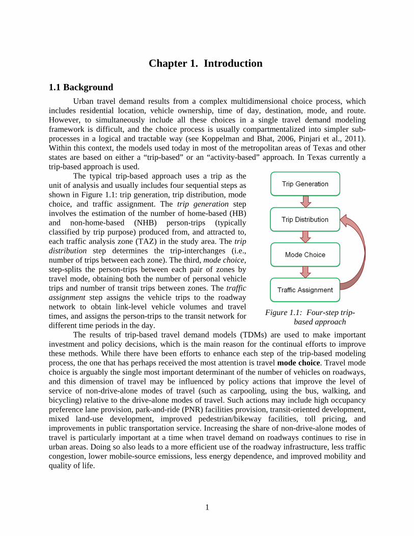
The typical trip-based approach uses a trip as the unit of analysis and usually includes four sequential steps as shown in Figure 1.1: trip generation, trip distribution, mode choice, and traffic assignment. The trip generation step involves the estimation of the number of home-based (HB) and non-home-based (NHB) person-trips (typically classified by trip purpose) produced from, and attracted to, each traffic analysis zone (TAZ) in the study area. The trip distribution step determines the trip-interchanges (i.e., number of trips between each zone). The third, mode choice, step-splits the person-trips between each pair of zones by travel mode, obtaining both the number of personal vehicle trips and number of transit trips between zones. The traffic assignment step assigns the vehicle trips to the roadway network to obtain link-level vehicle volumes and travel times, and assigns the person-trips to the transit network for different time periods in the day.

Figure 1.1: Four-step trip-based approach

The results of trip-based travel demand models (TDMs) are used to make important investment and policy decisions, which is the main reason for the continual efforts to improve these methods. While there have been efforts to enhance each step of the trip-based modeling process, the one that has perhaps received the most attention is travel mode choice. Travel mode choice is arguably the single most important determinant of the number of vehicles on roadways, and this dimension of travel may be influenced by policy actions that improve the level of service of non-drive-alone modes of travel (such as carpooling, using the bus, walking, and bicycling) relative to the drive-alone modes of travel. Such actions may include high occupancy preference lane provision, park-and-ride (PNR) facilities provision, transit-oriented development, mixed land-use development, improved pedestrian/bikeway facilities, toll pricing, and improvements in public transportation service. Increasing the share of non-drive-alone modes of travel is particularly important at a time when travel demand on roadways continues to rise in urban areas. Doing so also leads to a more efficient use of the roadway infrastructure, less traffic congestion, lower mobile-source emissions, less energy dependence, and improved mobility and quality of life.

2

1.2 Objective of Research Project

In the above context of focusing on solutions to manage growing travel demand in urban areas in Texas, the Texas Department of Transportation (TxDOT) Transportation Planning and Programming (TPP) Division is initiating another enhancement of their travel demand modeling system so that they can analyze alternative transportation modes (carpooling, public transportation, bicycling/walk modes) and evaluate (and prioritize) multimodal projects at the regional level.

TxDOT created a standardized approach for travel demand modeling called the Texas Package Suite (Sener et al., 2009) of Travel Demand Models (referred to as the Texas Package). The Texas Package, in conjunction with TransCAD, is a three-step daily vehicle-trip-based model. The three steps included in the Texas Package are trip generation, trip distribution, and traffic assignment. The Texas Package has been used since the late 1990s statewide, but TxDOT is looking into the possible inclusion of mode choice models for MPOs with the need for one.

Currently, TxDOT-TPP is responsible for TDM development to support the regional long-range plan update and associated long-range planning activities within 22 of the 25 Texas urban areas. The three Texas metropolitan planning organizations (MPOs) that TxDOT-TPP does not assist with model development are the Dallas/Fort Worth, El Paso, and Houston-Galveston MPOs; however, TxDOT-TPP does have a technical advisory or oversight role with the El Paso MPO. Among the 25 Texas MPOs, only four urban areas (Austin, Dallas/Fort Worth, Houston, and San Antonio) currently have developed a travel mode choice model (see Figure 1.2). The remaining urban areas do not have a mode choice modeling step in their TDM systems. At the same time, many of the 21 small and medium urban areas that do not have a mode choice step have been experiencing significant demographic population growth in the past decade. This growth motivates TxDOT-TPP’s efforts to develop a mode choice model that would be applicable for small and medium-sized MPOs.

3

Figure 1.2: Texas MPOs with a travel mode choice component in their TDM

MPOs in Texas have been classified into four population-based categories:

• Small MPOs: population between 50,000 and 200,000

• Medium/small-sized MPOs: population between 200,001 and 500,000

• Medium/large-sized MPOs: population between 500,001 and 1,000,000

• Large MPOs: population greater than 1,000,000

This categorization is based on the National Cooperative Highway Research Program (NCHRP) Report 716 (NCHRP, 2012), and allows us to compare Texas MPOs with other U.S. MPOs. The categories and corresponding classification are presented in Table 1.1

MPOs with a travel mode choice model

4

Table 1.1: Population-based classification of Texas MPOs

Category Population

2010* MPO Name

Small MPOs (population

between 50,000 and 200,000)

92,565 Texarkana MPO 111,823 San Angelo MPO (SAMPO) 115,384 Victoria MPO 120,877 Sherman-Denison MPO 151,306 Wichita Falls MPO 165,252 Abilene MPO 173,278 Harlingen-San Benito MPO

Medium/small-sized MPOs

(population between 200,001 and 500,000)

209,714 Tyler Area MPO 214,369 Longview MPO 228,660 Bryan-College Station MPO (BCSMPO) 234,906 Waco MPO 241,831 Brownsville MPO 249,881 Amarillo MPO 250,304 Laredo MPO 274,002 Midland-Odessa Transportation Organization (MOTOR) 284,890 Lubbock MPO (LMPO) 388,745 South East Texas Regional Planning Commission (SETRPC) 405,300 Killeen-Temple MPO (KTMPO) 428,185 Corpus Christi MPO

Medium/large-sized MPOs

(population 500,001 to 1,000,000)

774,769 Hidalgo County MPO (HCMPO) 800,647 El Paso MPO

Large MPOs (population greater

than 1,000,000)

1,716,289 Capital Area MPO (CAMPO) 2,142,508 San Antonio-Bexar County MPO (SABCMPO) 5,946,800 Houston-Galveston Area Council (HGAC) 6,371,773 North Central Texas Council of Governments (NCTCOG)

*Source: Texas State Data Center (2011)

This report is divided into nine chapters and has five appendices, including the guide with

instructions for running the model. The Forecasting Tool User Manual in Appendix B is also a stand-alone document (0-6766-P1). Chapter 1 is an introduction to the project. Chapter 2 provides a literature review of mode choice models. Chapter 3 discusses how to incorporate a model choice model into a smaller/medium-sized MPO and Chapter 4 outlines how to develop a forecasting approach and model design. Chapter 5 outlines the procedure to develop skims, with Chapter 6 reviewing the procedures used to develop transit skims in four medium and small MPOs in Texas. Chapter 7 outlines the procedure to prepare data for use in the model and Chapter 8 describes the model development and guide to utilizing the model. Chapter 9 provides conclusions and recommendations for future work.

5

Chapter 2. Literature Review

The initial task of the research study was to synthesize the available literature on mode choice models and develop an approach to assess the appropriateness of implementing a mode choice model in small and medium-sized Texas MPOs. This task also made recommendations regarding the incorporation of a mode choice step in Texas’ small and medium-sized MPOs.

U.S. and Texas MPOs were reviewed to assess whether they have already estimated, calibrated, and validated mode choice models. The research team opted to focus on developing a framework only for home-based (HB) trips to work. This decision was reached mainly because in urban areas, much emphasis has been placed on modeling mode choice for HB work trips, primarily driven by the concentration of such trips during the morning and evening rush hours. This decision was also taken because the primary audience for this research is TxDOT and Texas MPOs, who are evaluating the need (and therefore, procedures) for integrating a mode choice model into their TDM. The synthesis however, may also be useful to technical staff at other state Departments of Transportation (DOTs), MPOs, transit agencies, and planning agencies involved in travel demand modeling.

The objectives of this initial task were to

1) investigate the general methods and procedures adopted by MPOs across the U.S. that have incorporated a mode choice component into their TDMs. Specific issues of interest include the alternative conceptual structures; inputs/outputs and the model formulation; the steps taken to develop and implement mode choice models; model estimation, calibration, and validation procedures; and model application procedures;

2) identify the challenges faced in the model development and application, and document lessons learned; and

3) develop an approach to assess the appropriateness of implementing a mode choice model for a specific urban area based on modal shares and the range of transportation planning needs, policy questions, project evaluations, and travel demand forecasting exercises being considered.

The remainder of this chapter is organized as follows. Sections 2.1 through 2.3 provide

an overview of the current practices in mode choice modeling in the U.S., with a particular emphasis on Texas MPOs. Section 2.4 develops an approach to assess the need to incorporate a mode choice component into the TDM of small and medium-sized MPOs in Texas. The final section of this chapter summarizes salient findings.

2.1 Mode Choice Models

2.1.1 Overview

Mode choice models provide the means to evaluate the ability of traffic congestion mitigation efforts to effect a change in travelers’ mode of travel from solo-auto to high-occupancy vehicles and non-motorized modes of travel. Koppelman and Bhat (2006) developed a self-instructing manual on travel mode choice analysis that is now widely used by practitioners in the consulting arena as well as at MPOs. As Koppelman and Bhat (2006) indicate, some of the common types of independent (or exogenous) variables used to explain individual mode choice

6

behavior include traveler characteristics, trip characteristics, and transportation system characteristics (see Table 2.1). The models are separately estimated by trip purposes, and sometimes further segmented (based on statistical and intuitive considerations) by traveler and trip characteristics or time periods. This approach is used because the motivations, preferences, and modal choices for an HB work trip are very different from those for an HB shopping trip. To estimate such models, urban household travel surveys (of the type conducted by TxDOT or TxDOT-TPP) are used to obtain information on trip mode choice, traveler characteristics, and trip purpose characteristics, while supplementary land-use and transportation system data are used to generate origin-destination (O-D) characteristics and transportation system characteristics (these are typically developed at the level of the TAZ, and appended to trips based on the origin and destination TAZs of each trip).

Table 2.1: Common variables used in travel mode choice models Factors influencing

mode choice Examples

Traveler characteristics

- Individual demographics (age, gender) - Household socio-demographics (income, number of workers, number

of adults, auto ownership level) - Household structure (single adult, nuclear family)

Trip characteristics

- Trip purpose (HB work, HB non-work, NHB) - O-D characteristics (area types of origins and destinations, built

environment measures at the origin and destination end, distance between origin and destination)

Transportation system characteristics

- Total travel time, out-of-vehicle travel time (OVTT), in-vehicle travel time (IVTT) for each travel mode

- Total travel cost for each travel mode, and parking costs for auto modes

- Presence and number of transfers for transit - Walk access and egress time for transit and walk access distance to

transit (used to determine transit availability)

In estimating mode choice models, four elements are important to consider: the decision-maker, the alternatives, the attributes of alternatives, and the decision rule.

1. Decision-maker: The decision-maker is a respondent in the survey, who is observed to make a choice of mode for one or more trips (of a specific purpose).

2. Alternatives: Individuals make a choice from a set of alternatives available to them. The availability of an alternative for an individual in the context of travel mode choice may be determined by legal regulations (a person cannot drive alone until the age of 16) or the non-availability of a vehicle. It also is typical to assume in mode choice models that transit (e.g., bus) is an available mode for an individual only if the transit stop is within 0.25 miles of the origin end and the destination end.

3. Attributes of the alternatives: The alternatives in a choice process are characterized by a set of attribute values, as encountered by a specific individual. Attributes include the transportation system characteristics such as travel times and costs.

7

4. Decision rule: A decision rule is a mechanism to process information and to evaluate alternatives. Traditional mode choice models are based on utility maximization theory, which assumes that, when faced with a choice of multiple alternatives, individuals will choose the alternative that provides them the highest level of value or attractiveness or utility (referred to as utility maximization). The utility associated with an alternative has two components: a deterministic (or observable) component that represents the portion of the utility observed by the analyst (and is a function of the attributes of the alternatives and the characteristics of the decision-maker), and an unknown (or unobserved) component that can be the result of many sources (imperfect information, measurement errors, omission of modal attributes, and omission of the characteristics of the individual that influence his/her choice). Two of the most commonly used utility maximizing models are the multinomial logit (MNL) model and the nested logit (NL) model (see Appendix A and B for details).

2.2 Mode Choice Models Outside of Texas

The TDMs of the following five MPOs outside of Texas with emphasis on the mode choice model component were reviewed:

• Champaign County Regional Planning Commission (CCRPC, Illinois)

• Lincoln MPO (Nebraska)

• Genesee County Metropolitan Planning Commission (GCMPC, Michigan)

• Association of Monterey Bay Area Governments (AMBAG, California)

• Metro MPO (Washington)

These MPOs were chosen to represent the four population-based categories defined in Table 1.1 (the medium/small-sized category had two representative MPOs). All MPOs presented in this section use a trip-based approach for the TDM with TAZs as the unit of analysis, and their TDM has a feedback process between the traffic assignment and trip distribution steps. A summary of the MPOs’ TDMs is presented in Table 2.2 (detailed descriptions are available in Appendix D).

The five MPOs listed in Table 2.2 disaggregate trips by purpose because, as mentioned before, travelers may have different mode preferences in different choice occasions. The small MPO (CCRPC) considers five trip purposes, while the medium and large MPOs consider seven to nine trip purposes. Trip production models are similar among MPOs. All MPOs develop a cross-classification model to estimate trip productions, although each MPO uses different explanatory variables (see Appendix D for details). Methodological differences arise for trip attractions. Trips attractions are computed based on other estimates (NCHRP Report 365), previous models, or linear regressions. Gravity models are used by all MPOs in the trip distribution step, except for Metro MPO, which does not have an independent trip distribution model.

8

Table 2.2: TDMs of MPOs outside of Texas

MPO Base year

Trip purposes

Trip generation models Trip distribution

model Trip

production Trip attraction

CCRPC (small MPO)

2002–2003

HB work, HB school, HB shopping, HB other, NHB

Cross classification

NCHRP Report 365

Gravity model

Lincoln MPO (medium/small-

sized MPO) 2009

HB work, HB shop, HB recreation, HB university,

HB other, work-based other, NHB


Earlier model results

Gravity model

GCMPC (medium/small-

sized MPO) 2005

HB work low income, HB work high income, HB

shopping, HB other, HB school, HB university, NHB

other, NHB work


Linear regression

model Gravity model

AMBAG (medium/large-

sized MPO) 2005

HB work, HB maintenance, HB discretionary, work-

based, HB school, visitors, others


From survey data (if

available); otherwise

NCHRP Report 365

Gravity model

Metro MPO (large MPO)

2008

HB work, HB shopping, HB recreation, HB other, NHB work, NHB non-work, HB

college, HB school


No longer computed

except for HB work and HB

college

Destination choice model

using MNL (no trip distribution

model)

A summary of the mode choice models of MPOs outside of Texas is presented in Table

2.3. Several differences in both methodology and data usage are clear from the information presented in the table. First, all MPOs disaggregate trips by purpose; however, these purposes are not the same as those used in the previous TDM steps (generation and distribution steps). The MPOs with a large number of trip purposes in the earlier steps aggregate the trips in only three purposes in the mode choice step: HB work, HB other, and NHB. Additionally, two MPOs disaggregate trips by either transit availability scores (Lincoln MPO classifies zones based on transit coverage and operations) or time periods. Second, smaller MPOs tend to use fewer data inputs and choice alternatives than do larger MPOs. Finally, Table 2.3 notes the use of a variety of mode choice model structures, including the MNL and NL models (see Appendices A and B) and a simple fixed percentage mode split model.

9

Table 2.3: Mode choice models of MPOs outside of Texas

MPO Disaggregation

level Data inputs Model Choice alternatives

CCRPC (small MPO)

5 trip purposes, 4 area types

Transit network characteristics, transit

impedance, mode attributes

MNL

1) Drive alone 2) Shared ride 3) Transit 4) Bike 5) Walk

Lincoln MPO (medium/small-sized MPO)

7 trip purposes, 5 transit availability zone scores (for

transit only)

Trip distance, boarding data, auto occupancy

Fixed percentage

1) Non-motorized 2) Transit 3) Auto

GCMPC (medium/small-sized MPO)

3 trip purposes (HB work, HB other,

NHB)

IVTT, OVTT, transit fare, trip distance, socio-economic characteristics

NL

1) Drive alone 2) Share ride 3) Transit 4) Bike 5) Pedestrian

AMBAG (medium/large -sized MPO)


NHB)

In-vehicle time, walk time, wait time, fare,

value of time, trip distance, number of transfers, transit fare

NL

1) Drive alone 2) Share ride 2-person 3) Shared ride 3+ person 4) Premium transit service 5) Local transit service 6) Park and ride (PNR) 7) Kiss and ride (KNR) 8) Non-motorized

Metro MPO (large MPO)


NHB), 2 time periods

In-vehicle time, walk time, wait time, fare,

number of transfers, trip distance, travel cost,

accessibility measures, household income,

number of workers per household, number of

vehicles per household, household size

MNL

1) Drive alone 2) Drive with passenger 3) Auto passenger 4) Bus only by walk access 5) LRT only by walk access6) Bus/LRT by walk access 7) Transit by PNR access 8) Bike 9) Walk

Following is a summary of the modelling approaches of these MPOs:

• CCRPC (CUUATS, 2009): Until recently, a fixed curve method was used for the mode choice step. In 2011, CCRPC updated their mode choice model to the MNL, using the five modes presented in Table 2.3. Three data sources were used to develop the MNL model: transit on-board survey data, local transit district routes, and ridership information data. The resulting model was validated, comparing the observed and estimated boardings, and trough transit screen-lines and cutline checks. The CCRPC case study highlights that modeling can benefit a small MPO by identifying these elements:

o the uses and benefits of travel demand forecasting on a regional basis.

o the resources necessary to develop, validate, maintain, and operate travel demand forecasting capabilities on a regional basis.

10

• Lincoln MPO (Lincoln MPO, 2011): In the mode choice step, Lincoln MPO uses a mode split approach, in which the percentage of non-motorized trips and transit trips are identified, with any remaining trips being classified as auto trips. The non-motorized shares were estimated using a distance-based algorithm model with data from the 2000 Census Transportation Planning Package (CTPP). The transit shares were obtained from transit ridership data, census “journey to work” data, and a sensitivity analysis of data from other areas. Finally, an auto occupancy model was used to separate the remaining trips into auto-driver or passenger-driver trips, based on the data from the CTPP. This last step was taken to convert person-trips from the trip generation and distribution models into vehicle trips for assignment to the roadway network.

• GCMPC (GCMPC, 2009): A three-level NL model is used for the mode choice step in the GCMPC area (see Figure 2.1). The model divides the person-trips into the five modes shown in the figure; only three trip purposes were estimated: HB work, HB other, and NHB. Travel counts, household travel survey data, and the 2007 transit on-board survey data were used to obtain the data inputs. The 2000 CTPP data was used as a reference for HB work trip as well. The entire TDM was validated using traffic counts. The nested structure was revisited and corrected to reach the acceptable error standards defined by the Michigan DOT. After the validation process, transit ridership estimates differed from the ridership counts by 25%.

Source: GCMPC (2009)

Figure 2.1: NL model structure of GCMPC’s mode choice model

• AMBAG (AMBAG, 2011): An NL model is used for the mode choice step (see Figure 2.2), estimated using data from the 2001–2002 Caltrans household survey. The model structure was updated to comply with the Federal Transit Administration (FTA) guidance for New and Small Starts forecasting, because some coefficients of the

11

previous mode choice model (for year 2000) were outside the accepted FTA range and the model had county-specific constants that are not allowed by the FTA. The model is a three-level structure for three trip purposes—HB work, HB other, and NHB—and divides the person-trips into the eight alternative modes highlighted in Figure 2.2. The explanatory variables included in the model are IVTT, OVTT, wait time, transfer wait time, number of transfers, operational cost, and parking cost. For transit-related characteristics, data was drawn from the transit network, which consists of a description of bus lines that are superimposed on the road network. Transit line characteristics include the locations of stops, walk access links, and peak and midday headways. Transit speed was obtained by adjusting the average speed of all vehicles by link. The TDM model was validated and a 40.75% root mean squared error was obtained for the predicted boardings.

Source: AMBAG (2011)

Figure 2.2: NL model structure of AMBAG’s mode choice model

• Metro MPO (Metro, 2008): An MNL model was used for the mode choice step. Metro’s model was applied to three trip purposes (HB work, HB other, and NHB) and two time periods (peak: 07:00–08:59AM; and off-peak: 14:00–14:59). The mode choice alternatives considered include the nine choice alternatives shown in Table 2.3. Household demographic variables and income-specific cost coefficients were used for the model specification. Accessibility measures include household, employment, and intersection density. Mode characteristics considered in the analysis include in-vehicle time, walk time, first wait time (modeled at 50% of headway), transfer wait time, and number of boardings. Bike and walk travel times are calculated based on assumed speeds.

2.3 Mode Choice Models in Texas

As mentioned in Section 2.1, each MPO in Texas is responsible for the transportation planning and programming coordination within their urban area. In this section we review the mode choice models developed by the four large MPOs in Texas: Capital Metro MPO (CAMPO), San Antonio-Bexar County MPO (SABCMPO), Houston-Galveston Area Council

12

(HGAC), and North Central Texas Council of Governments (NCTCOG). All urban areas use a four-step trip-based approach to model and forecast travel demand.

2.3.1 Capital Metro MPO (CAMPO)

CAMPO is the MPO for the Austin area, which includes the Bastrop, Caldwell, Hays, Travis, and Williamson counties. CAMPO has a four-step daily vehicle trip-based model: trip generation, trip distribution, mode choice, and traffic assignment. These are the basic steps of TxDOT’s Texas Package (described in Section 1.2) with the addition of the mode choice model step. CAMPO compiles their data from many sources.

They conduct surveys in household travel, workplace travel, commercial vehicle, external travel, and on-board transit. They also obtain 24-hour traffic counts, speed limit data, and demographical data to help validate the models. This data, along with that provided by TxDOT, allows CAMPO to run a successful model for their area.

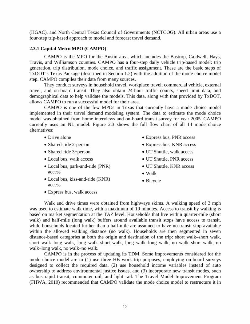
CAMPO is one of the few MPOs in Texas that currently have a mode choice model implemented in their travel demand modeling system. The data to estimate the mode choice model was obtained from home interviews and on-board transit survey for year 2005. CAMPO currently uses an NL model. Figure 2.3 shows the full flow chart of all 14 mode choice alternatives:

• Drive alone

• Shared-ride 2-person

• Shared-ride 3+person

• Local bus, walk access

• Local bus, park-and-ride (PNR) access

• Local bus, kiss-and-ride (KNR) access

• Express bus, walk access

• Express bus, PNR access

• Express bus, KNR access

• UT Shuttle, walk access

• UT Shuttle, PNR access

• UT Shuttle, KNR access

• Walk

• Bicycle

Walk and drive times were obtained from highways skims. A walking speed of 3 mph

was used to estimate walk time, with a maximum of 10 minutes. Access to transit by walking is based on market segmentation at the TAZ level. Households that live within quarter-mile (short walk) and half-mile (long walk) buffers around available transit stops have access to transit, while households located further than a half-mile are assumed to have no transit stop available within the allowed walking distance (no walk). Households are then segmented in seven distance-based categories at both the origin and destination of the trip: short walk–short walk, short walk–long walk, long walk–short walk, long walk–long walk, no walk–short walk, no walk–long walk, no walk–no walk.

CAMPO is in the process of updating its TDM. Some improvements considered for the mode choice model are to (1) use three HB work trip purposes, employing on-board surveys designed to collect the required data, (2) use household income variables instead of auto ownership to address environmental justice issues, and (3) incorporate new transit modes, such as bus rapid transit, commuter rail, and light rail. The Travel Model Improvement Program (FHWA, 2010) recommended that CAMPO validate the mode choice model to restructure it in

13

accordance with the FTA requirements, and to collect data on the commuter rail service for future usage.

2.3.2 Houston-Galveston Area Council (HGAC)

The study area for HGAC encompasses eight counties: Montgomery, Liberty, Chambers, Galveston, Brazoria, Fort Bend, Waller and Harris. HGAC develops its TDM in collaboration with TxDOT and the Metropolitan Transit Authority of Harris County (METRO). In the trip generation step, trips are categorized into 14 purposes. The trip household production models use cross-classification trip production rates developed from the HGAC 1995 Household Travel Survey data, while the trip attraction rates are stratified by area type and employment category. An atomistic model is used for the trip distribution step (HGAC, 2012).

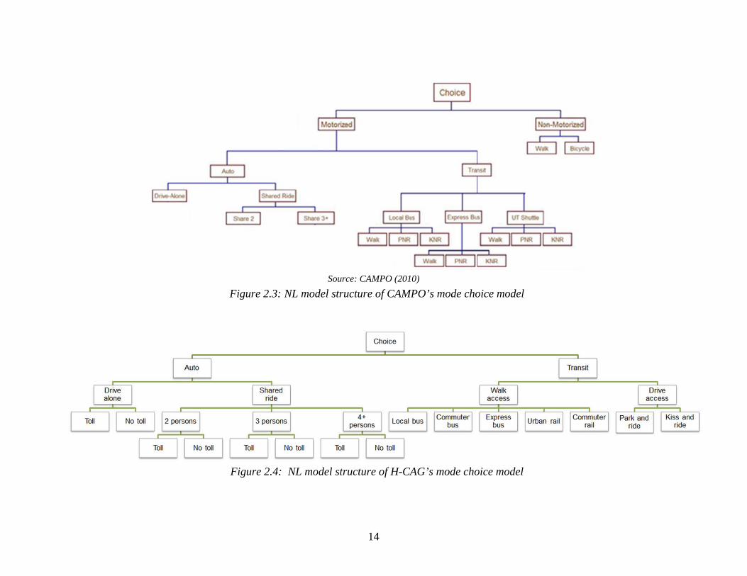
The development of the HGAC mode choice model was based on the 1995 household survey data and on-board transit rider survey data. HGAC updated its previous mode choice model (an NL model) with a new NL model that encompasses more alternatives than the previous model and a different nesting structure. Additionally, separate NL models were developed for five income groups and three trip purposes (HB work, HB non-work, and NHB). The model includes 15 alternatives as follows:

• Drive alone non-toll

• Drive alone toll

• Two person auto non-toll

• Two person auto toll

• Three person auto non-toll

• Three person auto toll

• Four-plus person auto non-toll

• Four-plus person auto toll

• Transit-walk access commuter bus

• Transit-walk access local bus

• Transit-walk access express bus

• Transit-walk access urban rail

• Transit-walk access commuter rail

• Transit-drive access PNR

• Transit-drive access KNR

All mode choice models estimated had the same specification and nesting structure (see Figure 2.4). The explanatory variables used are IVTT, wait time (two categories: less than 4.5 minutes and greater than 4.5 minutes), walk time, transfer time, number of transfers, transit fare, drive to transit time, parking cost, highway operating cost, tolls, and residential density factor.

14

Source: CAMPO (2010)

Figure 2.3: NL model structure of CAMPO’s mode choice model

Figure 2.4: NL model structure of H-CAG’s mode choice model

15

The model validation process showed that the number of highway trips (obtained from auto trips) was lower than expected, because of inconsistencies in number of occupants per vehicle. Then, the HB non-work and NHB models were modified: auto costs were no longer shared among vehicle occupants, and an additional household size variable was added to the models. Finally, the models were applied at the TAZ level and the mode specific constants were adjusted to match observed 1995 control values. This last step was required for forecasting purposes.

2.3.3 San Antonio-Bexar County MPO (SABCMPO)

The study area for the San-Antonio encompasses five counties: Bexar, Comal, Guadalupe, Kendall, and Wilson. The development of the 2005 TDM represents a cooperative effort among the SABCMPO, Alamo Area Council of Governments, VIA Metropolitan Transit Authority, and TxDOT and its TPP Division. Productions and attractions are estimated using TxDOT’s TRIPCAL5 trip generation modeling software package, and the trip distribution step is undertaken using TxDOT’s Atom 2 gravity model distribution package (SABCMPO, 2011).

For the San Antonio region, a series of comprehensive travel surveys were conducted during 2005–2006 to update their TDM; in particular, household travel survey data was utilized for the development of the mode choice model. A total of seven alternatives were considered:

• Drive alone

• Shared ride (two-person carpool)

• Shared ride (three-person carpool)

• Bus (walk access)

• Bus separate (drive access or PNR)

• Bicycle

• Walk

SABCMPO’s mode choice model estimates the person-trips by travel mode at the zonal level by taking into consideration characteristics of the traveler and available highway and transit services. Different mode choice models were for different time periods, categorized as peak (6:30–9:00 AM and 3:00–6:00 PM) and off-peak (all other time periods of the day), and three trip purposes (HB work, HB other, and NHB). An NL model was used for the mode choice model (see Figure 2.5). A wide range of explanatory variables were considered in the model, including IVTT and OVTT, income, travel cost, wait time, number of transfers, and parking cost. Some parameter values were fixed in order to facilitate consistent model estimation, including IVTT (parameter fixed to 1.0), wait time, transfer time, walk access time, walk egress time, transfer penalty time (all parameters fixed to 2.5), and cost (parameter fixed to 0.06). The TDM validation process showed that the model replicates base year travel for both highway and transit modes.

16

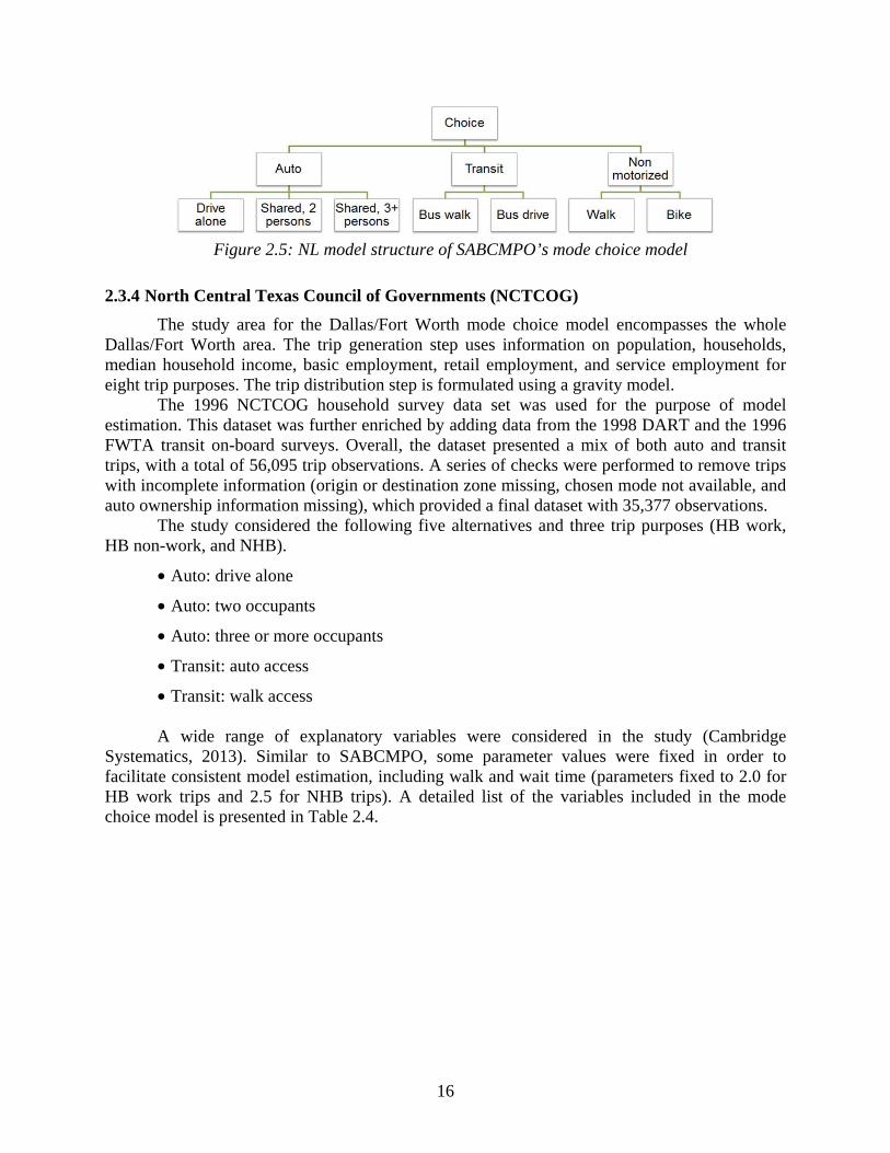
Figure 2.5: NL model structure of SABCMPO’s mode choice model

2.3.4 North Central Texas Council of Governments (NCTCOG)

The study area for the Dallas/Fort Worth mode choice model encompasses the whole Dallas/Fort Worth area. The trip generation step uses information on population, households, median household income, basic employment, retail employment, and service employment for eight trip purposes. The trip distribution step is formulated using a gravity model.

The 1996 NCTCOG household survey data set was used for the purpose of model estimation. This dataset was further enriched by adding data from the 1998 DART and the 1996 FWTA transit on-board surveys. Overall, the dataset presented a mix of both auto and transit trips, with a total of 56,095 trip observations. A series of checks were performed to remove trips with incomplete information (origin or destination zone missing, chosen mode not available, and auto ownership information missing), which provided a final dataset with 35,377 observations.

The study considered the following five alternatives and three trip purposes (HB work, HB non-work, and NHB).

• Auto: drive alone

• Auto: two occupants

• Auto: three or more occupants

• Transit: auto access

• Transit: walk access

A wide range of explanatory variables were considered in the study (Cambridge Systematics, 2013). Similar to SABCMPO, some parameter values were fixed in order to facilitate consistent model estimation, including walk and wait time (parameters fixed to 2.0 for HB work trips and 2.5 for NHB trips). A detailed list of the variables included in the mode choice model is presented in Table 2.4.

17

Table 2.5: List of explanatory variables in NCTCOG mode choice model

Characteristics Variables considered

Level of service variables

Auto travel time

Total transit travel time

Auto out-of-vehicle time

Transit walk access time

Transit wait time

Transit transfer time

Auto access time (transit auto access only)

Walk egress time (transit mode only)

Transit out-of-vehicle time

Fare

Auto operating cost

Parking cost

Sum of operating and parking cost (auto mode only)

Number of transfers (transit mode only)

Zonal variables

Population density at the production zone

Employment density at the attraction zone

Type of attraction zone (central business district, other business district, suburb, urban, rural)

Household variables

Income (3 categories: less than $30K, between $30K and $75K, greater than $75K)

Number of autos in household

Number of persons in household

Auto Indicator: 1 if fewer autos in household than person, 0 otherwise

NL models were developed for all HB (work and non-work) purposes, and an MNL was

used for NHB trips. However, different nesting definitions and explanatory variables were used for each trip purpose. Figure 2.6 presents the nesting structures used by NCTCOG. Several constraints were imposed during the estimation process. For HB work trips, transit fare coefficient and auto fare coefficient were set to -0.550 and -0.770, to match the national averages. For HB non-work trips, auto in-vehicle time coefficient and transit fare coefficient were constrained to -0.016 and -0.008, respectively. For NHB trips, the auto and transit IVTT were constrained to -0.011 and -0.007, respectively. Similarly, the cost coefficient for two modes were set to -0.200.

18

Figure 2.6: NL model structure of NCTCOG’s mode choice model

HB work trips

HB non-work trips

19

Chapter 3. Incorporating a Mode Choice Component for Small and Medium-Sized MPOs in Texas

To assess whether it is appropriate to implement a mode choice component in small and medium-sized MPOs in Texas, three factors were considered:

1. Population growth: According to the U.S. Census Bureau (2011), the state’s population has increased by 20.6% between 2000 and 2010. This increase translates into 4.3 million people. From a transportation planning perspective, this rapid population growth is associated with more vehicles in the roadways and, therefore, increased travel times, traffic congestion, and greenhouse gas emissions. The incorporation of a mode choice component in the TDM could help MPOs to understand and control the effects of a fast-growing population.

2. Mode choice shares: Texas’ transportation systems are integral to the state’s economic and functional viability and vibrancy, providing accessibility for the daily travel needs of residents and tourists, freight shipments, and commuting trips. While both roadways and public transportation systems are important to providing services for all residents, more than 91% of Texas commuters use a personal automobile or carpool to get to work. On the other hand, less than 2% of commuters use the public transportation system and non-motorized forms of transportation (U.S. Census Bureau, 2009). However, in some urban areas in Texas the use of alternative transportation modes is more widespread; therefore, these areas may benefit from the inclusion of a mode choice component in their TDM.

3. Strategic planning goals: Transportation planning involves identifying broad regional problems and challenges that the region expects to face over the next years. In long-range transportation plans, also referred as Metropolitan Transportation Plans (MTPs), MPOs usually define their long-term goals and strategies. Because transportation is interconnected with health, quality of life, social equity, and the environment, several of these goals are strictly related to promoting the use of alternative transportation modes. To examine the potential impact of such policies, developing a travel mode choice model is important.

The population growth, modal shares, and types of policies being considered in the urban

areas will shape the need for, and the structure of, travel mode choice models. In the following sections, we describe each factor in the context of small and medium-sized MPOs in Texas.

3.1.1 Population Growth

Table 3.1 presents small and medium-sized MPOs’ area and population. As the table illustrates, Texas MPOs vary widely in both the spatial area and population they serve. Many small and medium-sized MPOs (for example, Hidalgo County MPO, Laredo MPO, and Bryan-College Station MPO) have experienced significant growth in the past decade, growing at even higher rates than the state average. Overall, small MPOs tend to have a percentage growth smaller than medium-sized MPOs.

20

Table 3.1: MPO population growth

MPO 2000

Population 2010

Population Population growth (%)

Small MPOs

Texarkana MPO 89,306 92,565 3.65 San Angelo MPO 105,781 111,823 5.71 Victoria MPO 111,663 115,384 3.33 Sherman-Denison MPO 110,595 120,877 9.30 Wichita Falls MPO 151,524 151,306 -0.14 Abilene MPO 160,245 165,252 3.12 Harlingen-San Benito MPO 144,658 173,278 19.78


Tyler Area MPO 174,706 209,714 20.04 Longview MPO 194,042 214,369 10.48 Bryan-College Station MPO 184,885 228,660 23.68 Waco MPO 213,517 234,906 10.02 Brownsville MPO 190,569 241,831 26.90 Amarillo MPO 226,522 249,881 10.31 Laredo MPO 193,117 250,304 29.61 Midland-Odessa Transportation Organization 237,132 274,002 15.55 Lubbock MPO 249,700 284,890 14.09 South East Texas Regional Planning Commission 385,090 388,745 0.95 Killeen-Temple MPO 330,714 405,300 22.55 Corpus Christi MPO 403,280 428,185 6.18


Hidalgo County MPO 569,463 774,769 36.05 El Paso MPO 679,622 800,647 17.81

Source: Texas State Data Center (2011)

3.1.2 Mode Choice Shares

To obtain a sense of modal shares in the Texas small and medium-sized urban areas, the CTR team extracted information from the 2009 American Community Survey, and obtained modal shares for work trips for the 21 MPOs that currently have not implemented mode choice models within their travel demand modeling framework (see Table 3.2). Not surprisingly, the vast majority of work trips in each urban area are pursued by driving alone (82.42% on average across the 21 urban areas) or carpooling (12.62% on average). In several urban areas (Denison, Texarkana, Midland, Temple, and Port Arthur), the percentage of commuters that rely on the automobile (by driving alone or carpooling) to reach their workplace exceeds 97%. Only in three urban areas (College Station, El Paso, and Laredo) does the public transportation share exceed 1.5%. College Station registers the highest share of non-motorized mode share (6.42%), attributable to special generator trips from the Texas A&M College campus.

21

Table 3.2: Mode shares for HB work trips

MPO Area Modal Share [%]

Drive alone

Carpool Transit Bike Walk Other

Small MPOs

Texarkana MPO Texarkana 85.43 11.81 0.23 0.00 1.55 0.97

San Angelo MPO San Angelo 81.46 11.01 0.61 0.06 5.00 1.86

Victoria MPO Victoria 80.16 15.53 0.78 0.34 1.95 1.24

Sherman-Denison MPO Denison 88.15 10.37 0.32 0.46 0.70 0.00

Sherman 83.91 12.90 0.22 0.00 1.10 1.86

Wichita Falls MPO Wichita Falls 80.86 10.71 0.48 0.00 6.79 1.15

Abilene MPO Abilene 84.38 11.41 0.39 0.40 2.19 1.23

Harlingen-San Benito MPO Harlingen 86.02 10.84 0.06 0.42 1.25 1.40


Tyler Area MPO Tyler 84.65 11.01 0.57 0.18 0.97 2.62

Longview MPO Longview 84.93 11.27 0.21 0.13 1.40 2.06

Bryan-College Station MPO

Bryan 83.62 11.53 1.31 0.34 1.02 2.19

College Station 78.25 10.42 3.84 2.52 3.90 1.08

Waco MPO Waco 82.79 13.13 0.30 0.21 2.80 0.78

Brownsville MPO Brownsville 78.50 14.52 1.26 0.08 2.71 2.93

Amarillo MPO Amarillo 84.76 11.80 0.39 0.14 1.63 1.27

Laredo MPO Laredo 77.86 15.96 1.97 0.06 2.42 1.73

Midland-Odessa MPO Midland 85.21 12.51 0.32 0.02 0.95 0.99

Odessa 82.22 14.02 0.23 0.14 1.57 1.82

Lubbock MPO Lubbock 85.57 10.72 0.67 0.29 2.12 0.63

South East Texas RPC Beaumont 85.42 10.81 0.97 0.17 1.79 0.83

Port Arthur 84.60 12.60 0.37 0.17 1.54 0.71

Killeen-Temple MPO

Fort Hood CDP 80.26 11.77 0.14 0.02 6.09 1.72

Killeen 82.21 14.33 0.38 0.10 1.56 1.41

Temple 85.22 11.91 0.28 0.04 0.96 1.59

Corpus Christi MPO Corpus Christi 79.64 13.80 1.34 0.34 2.05 2.84


Hidalgo County MPO

Edinburg 77.00 15.48 0.19 0.61 1.66 5.05

McAllen 84.00 11.73 0.71 0.05 1.22 2.30

Mission 74.56 16.17 0.00 0.00 0.71 8.56

El Paso MPO El Paso 82.06 11.37 1.85 0.16 2.27 2.29

Average 82.42 12.62 0.71 0.28 2.00 1.97

Std. Deviation 3.21 1.83 0.80 0.47 1.45 1.62

Minimum 74.56 10.37 0.00 0.00 0.70 0.00

Maximum 88.15 16.17 3.84 2.52 6.79 8.56

Source: U.S. Census Bureau, American Community Survey 2009

22

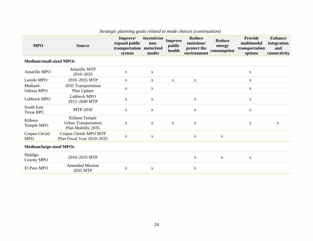
3.1.3 Strategic Planning Goals

Table 3.3 summarizes the strategic planning goals of the 21 small and medium-sized MPOs in Texas. The information presented in the table was obtained from the MPOs’ MTPs. In order to assess if the MPOs have goals that align with multimodality, the CTR research team classified the goals into the following categories:

• Improve and/or expand public transportation system

• Incentivize non-motorized modes

• Improve public health

• Reduce emissions and/or protect the environment

• Reduce energy consumption

• Provide multimodal transportation options

• Enhance integration and connectivity

Several observations may be drawn from the information in the table. First, all MPOs seek to improve and/or expand the public transportation system (train and bus) in the future, except for the Abilene, Brownsville, and Hidalgo County MPOs. Second, most MPOs encourage the use of non-motorized modes by adding on-street bike lanes, off-street multi-use paths, and signed bicycle routes for bike mode choice, and designing a network of sidewalks and multi-use paths to accommodate pedestrians’ mode choice. However, only few MPOs articulate intent to improve public health in the long-range transportation plan. Most of them are concentrating on protecting the environment and improving the air quality to meet the National Ambient Air Quality Standards established by the Environmental Protection Agency. Finally, since most MPOs target development of transportation modes other than drive-alone, the provision of multimodal transportation options is quite common.

23

Table 3.3: Strategic planning goals related to mode choices

MPO Source

Improve/ expand public transportation

system

Incentivize non-

motorized modes

Improve public health

Reduce emissions/ protect the

environment

Reduce energy

consumption

Provide multimodal

transportation options

Enhance integration

and connectivity

Small MPOs

Texarkana MPO

Texarkana Urban Transportation Study

2035 Plan x x x x

San Angelo MPO

MTP Fiscal Years 2010–2035

x x x

Victoria MPO Victoria Urbanized

Area MTP 2035 x x x x x x x

Sherman-Denison MPO

Transportation Outlook: 2035

x x x

Wichita Falls MPO

2010–2035 MTP x x

Abilene MPO Abilene Metropolitan Area

MTP 2010–2035 x x x x x

Harlingen-San Benito MPO

2010–2035 MTP x x x x x x


Tyler Area MPO

MTP 2035 x x x x

Longview MPO

MTP 2035 x x x x

Bryan-College Station MPO

Bryan/College Station MPO 2010–2035 MTP

x x x x

Waco MPO Connections 2035:

The Waco MTP x x x x x

Brownsville MPO

2010–2035 Brownsville MTP x x x x x

24

Strategic planning goals related to mode choices (continuation)

MPO Source

Improve/ expand public transportation

system

Incentivize non-

motorized modes

Improve public health

Reduce emissions/ protect the

environment

Reduce energy

consumption

Provide multimodal

transportationoptions

Enhance integration

and connectivity


Amarillo MPO Amarillo MTP

2010–2035 x x x

Laredo MPO 2010–2035 MTP x x x x x Midland-Odessa MPO

2035 Transportation Plan Update

x x x

Lubbock MPO Lubbock MPO

2012–2040 MTP x x x x

South East Texas RPC

MTP-2030 x x x x

Killeen-Temple MPO

Killeen-Temple Urban Transportation Plan Mobility 2035

x x x x x x

Corpus Christi MPO

Corpus Christi MPO MTP Plan Fiscal Year 2010–2035

x x x x


Hidalgo County MPO

2010–2035 MTP x x x

El Paso MPO Amended Mission

2035 MTP x x x

25

3.2 Recommendations

Based on the information collected in Tables 3.1 to 3.3, Table 3.4 presents a recommendation on whether implementing a mode choice component has the prospect of adding substantial value, given the population growth trends, current modal splits, and future planning priorities at each small and medium-sized MPO in Texas.

• The first column classifies the population growth into three levels: large (population growth more than 20%), medium (population growth between 10% and 20%), and small (less than 10%).

• The second column, non-insignificant share of non-auto modes, evaluates whether the MPO non-drive-alone modal share is non-insignificant or not. A “yes” in the column means that the MPO has a non-auto mode share considerably higher than the average (across all MPOs).

• The third column evaluates whether the assessment of the MPO long-range policies will benefit from a mode choice analysis or not. A “yes” in the column conveys that the MPO has at least four strategic planning goals that are highly related to mode choices, making a model choice model more important to incorporate.

• The last column provides a recommendation on incorporating a mode choice model in the TDM. The assessment was defined in three levels:

- Not recommended: no diverse mode choices, medium to small population growth, goals do not relate to mode choice.

- Recommended: one or two of the following: diverse mode choices, large population growth, and goals highly related to mode choice analysis.

- Highly recommended: the MPO has diverse mode choices, large population growth, and goals highly related to mode choice analysis.

The literature review of mode choice models in MPOs outside of Texas shows several

differences in approaches. MPOs use a variety of models, although the MNL and NL models are the most prevalent. All MPOs developed different mode choice model for different trip purposes; HB work, HB non-work, and NHB were the most common categories used. The number and type of choice alternatives considered varies among MPOs, based mainly on region-specific characteristics.

In Texas, only four MPOs have developed a mode choice model. Among them, CAMPO and SABCMPO rely on TxDOT’s Texas Package for travel demand modeling. Therefore, their modeling approach can be adapted by small and medium-sized MPOs that also rely on the Texas Package for modeling purposes. The four MPOs use an NL model, but the number and type of alternatives vary among regions, along with differences in the manner of the disaggregation of trips by purpose and time period. The HGAC mode choice model is far more detailed in terms of the representation of modal alternatives. However, the NCTCOG mode choice model appears to use the most detailed data inputs, which could help to understand and predict mode choices more accurately.

26

Table 3.4: Recommendation on incorporating a mode choice model in the TDM

MPO Population

growth

Non-insignificant share of non-auto modes

Policy evaluation

needs mode choice analysis

Recommendation on incorporating a

mode choice model in the TDM

Small MPOs

Texarkana MPO Small Yes Recommended San Angelo MPO Small Yes Recommended Victoria MPO Small Yes Yes Recommended Sherman-Denison MPO Small Not recommended Wichita Falls MPO Small Yes Recommended Abilene MPO Small Yes Recommended

Harlingen-San Benito MPO Medium Yes Recommended


Tyler Area MPO Medium Yes Recommended Longview MPO Small Yes Recommended Bryan-College Station MPO Large Yes Yes Highly recommended Waco MPO Small Yes Recommended Brownsville MPO Large Yes Yes Highly recommended Amarillo MPO Medium Not recommended Laredo MPO Large Yes Yes Highly recommended Midland-Odessa MPO Medium Not recommended Lubbock MPO Medium Yes Recommended South East Texas RPC Small Yes Recommended Killeen-Temple MPO Large Yes Yes Highly recommended

Corpus Christi MPO Small Yes Yes Recommended


Hidalgo County MPO Large Yes Recommended

El Paso MPO Medium Yes Recommended

The development of a mode choice model is a process that requires time. Most MPOs, in

and outside Texas, have been developing mode choice model (and reevaluating them) for several years. Some MPOs, such as CAMPO, started with a highly restricted model specification (in terms of alternatives considered and data used), but are planning to improve the model for future TDMs. For most MPOs, the TDM validation process is quite helpful in discerning whether the mode choice model is correctly predicting mode shares and improving forecasting. From an implementation perspective, the small MPO reviewed (CCRPC) recognized that the development of TDMs (including the mode choice component) is a challenging task that requires identifying TDM’s uses and benefits and the resources necessary to develop, validate, maintain, and operate it.

Small and medium-sized MPOs in Texas were analyzed to assess the appropriateness of developing a mode choice model in their areas. Three variables were studied to make this assessment: population growth, modal shares, and strategic planning goals. As a result of this analysis, we highly recommend incorporating a mode choice model step in the TDM of 3 MPOs

27

(Bryan-College Station MPO, Laredo MPO and Killeen-Temple MPO), do not recommend implementing a mode choice model in 3 urban areas (Sherman-Denison MPO, Amarillo MPO, Midland-Odessa MPO), and recommend incorporating a mode choice model in the other 15 MPOs.

In conclusion, the private automobile’s dominance among travel modes used in Texas urban areas highlights the importance of developing the technical ability to evaluate multimodal projects that attempt to increase the shares of non-drive-alone modes of travel, such as public transportation and walking, to mitigate congestion and air quality issues. The implementation of a mode choice model in the TxDOT-TPP’s TDM can help in these efforts and also contributes to understanding unmet needs for local populations, an issue that is of substantial importance for addressing policy concerns related to equity, mobility, accessibility, and overall quality of life.

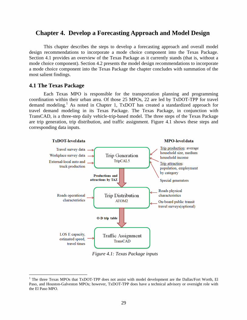
29

Chapter 4. Develop a Forecasting Approach and Model Design

This chapter describes the steps to develop a forecasting approach and overall model design recommendations to incorporate a mode choice component into the Texas Package. Section 4.1 provides an overview of the Texas Package as it currently stands (that is, without a mode choice component). Section 4.2 presents the model design recommendations to incorporate a mode choice component into the Texas Package the chapter concludes with summation of the most salient findings.

4.1 The Texas Package

Each Texas MPO is responsible for the transportation planning and programming coordination within their urban area. Of those 25 MPOs, 22 are led by TxDOT-TPP for travel demand modeling.1 As noted in Chapter 1, TxDOT has created a standardized approach for travel demand modeling in its Texas Package. The Texas Package, in conjunction with TransCAD, is a three-step daily vehicle-trip-based model. The three steps of the Texas Package are trip generation, trip distribution, and traffic assignment. Figure 4.1 shows these steps and corresponding data inputs.

Figure 4.1: Texas Package inputs

1 The three Texas MPOs that TxDOT-TPP does not assist with model development are the Dallas/Fort Worth, El Paso, and Houston-Galveston MPOs; however, TxDOT-TPP does have a technical advisory or oversight role with the El Paso MPO.

30

STEP 1: Trip generation predicts the numbers of trips originated in and destined to each TAZ using the software TripCAL5. Trip attractions and productions are calculated at the TAZ level. To calculate the trips produced (originating) and trips attracted (destination) to each TAZ, the MPO and TxDOT have to provide the data to be inputted into the software. The MPO provides zonal-based estimates of household size, household income, and median household income to compute trip productions. The MPO will also provide zonal household and employment by category to produce the trip attractions. The four basic employment categories used are basic, retail, service, and education. All of this information is obtained from conducting annual household surveys of the region. Then, this data is given to TxDOT, who estimates a matrix of households by size and income for each urban area and used as a constraint in TripCAL5. The MPO is also required to identify any special generators of traffic. Special generators are locations that have different travel characteristics than those found by trip generating models. This includes hospitals, colleges, and airports. TxDOT will acknowledge these special generators, but attempts to limit their use in trip generation models. TripCAL5 will then use all of these inputs to compute the productions and attractions by each TAZ for each trip purpose identified.

STEP 2: Trip distribution uses ATOM2, a spatially disaggregate trip distribution model, where an origin-destination (O-D) table is created that specifies the number of trips leaving each origin and arriving at each TAZ. To create individual trip tables, ATOM2 utilizes the productions and attractions generated by TripCAL5, as well as road features provided by the MPO and TxDOT. The MPO supplies information about the physical characteristics of the roads within each zone. This includes the number of lanes, posted speed limits, direction (one-way or two-way), functional classification, and their median access type (divided, undivided or continuous left turn). These characteristics are obtained from the transportation network database maintained by the MPO. TxDOT adds further information on road operational characteristics, including the area type, link capacity and speed, and link length. All of these road characteristics, supplied by the MPO and TxDOT, are then applied to create a matrix of network travel times from zone to zone. These inputs, with some additional information, are taken into the software to produce individual trip tables. These trip tables are then imported into TransCAD and altered into an O-D matrix, which is ultimately translated into 24-hour vehicle O-D trip tables.

STEP 3: Traffic assignment assigns the trips to the network using TransCAD. The traffic assignment models are based on a user equilibrium procedure and represent daily travel. Besides the 24-hour O-D trip table produced in the trip distribution step, other inputs are the Level of Service E Capacities and the travel times. No inputs in this step are provided by the MPO.

4.2 Mode Choice Model Recommendations

The literature review of mode choice models in MPOs in the U.S. in Chapter 2 showed that the MNL and NL models are the most prevalent. The models are separately estimated by trip purposes, and sometimes further segmented (based on statistical and intuitive considerations). To estimate such models, urban household travel surveys (of the type conducted by of TxDOT or TxDOT-TPP) are used to obtain information on trip mode choice, traveler characteristics, and trip purpose characteristics, while supplementary land-use and transportation system data are used to generate O-D characteristics and transportation system characteristics. Both MNL and NL models are derived from random utility maximizing behavior at the disaggregate level. Formally, the utility is as shown in Equation 4.1:

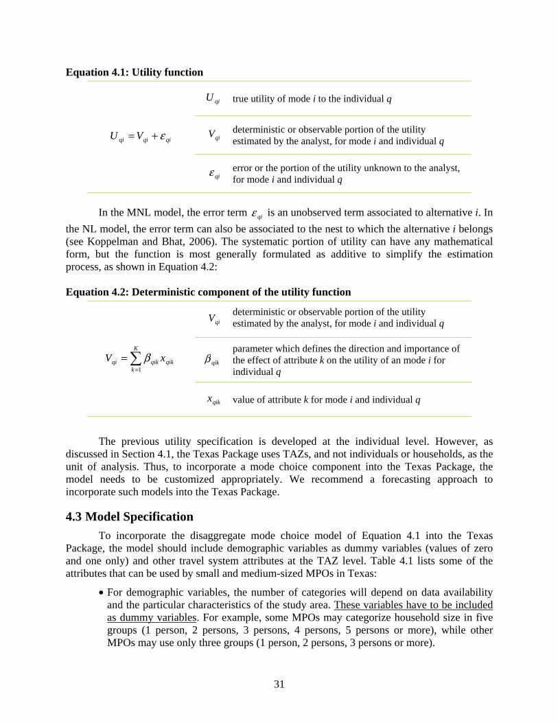
31

Equation 4.1: Utility function

qiqiqi VU ε+=

qiU true utility of mode i to the individual q

qiV deterministic or observable portion of the utility estimated by the analyst, for mode i and individual q

qiε error or the portion of the utility unknown to the analyst, for mode i and individual q

In the MNL model, the error term qiε is an unobserved term associated to alternative i. In

the NL model, the error term can also be associated to the nest to which the alternative i belongs (see Koppelman and Bhat, 2006). The systematic portion of utility can have any mathematical form, but the function is most generally formulated as additive to simplify the estimation process, as shown in Equation 4.2: Equation 4.2: Deterministic component of the utility function

=

=K

kqikqikqi xV

1

β

qiV deterministic or observable portion of the utility estimated by the analyst, for mode i and individual q

qikβ parameter which defines the direction and importance of the effect of attribute k on the utility of an mode i for individual q

qikx value of attribute k for mode i and individual q

The previous utility specification is developed at the individual level. However, as discussed in Section 4.1, the Texas Package uses TAZs, and not individuals or households, as the unit of analysis. Thus, to incorporate a mode choice component into the Texas Package, the model needs to be customized appropriately. We recommend a forecasting approach to incorporate such models into the Texas Package.

4.3 Model Specification

To incorporate the disaggregate mode choice model of Equation 4.1 into the Texas Package, the model should include demographic variables as dummy variables (values of zero and one only) and other travel system attributes at the TAZ level. Table 4.1 lists some of the attributes that can be used by small and medium-sized MPOs in Texas:

• For demographic variables, the number of categories will depend on data availability and the particular characteristics of the study area. These variables have to be included as dummy variables. For example, some MPOs may categorize household size in five groups (1 person, 2 persons, 3 persons, 4 persons, 5 persons or more), while other MPOs may use only three groups (1 person, 2 persons, 3 persons or more).

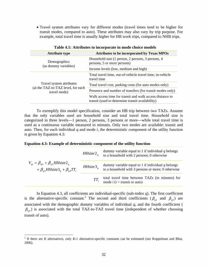
32

• Travel system attributes vary for different modes (travel times tend to be higher for transit modes, compared to auto). These attributes may also vary by trip purpose. For example, total travel time is usually higher for HB work trips, compared to NHB trips.

Table 4.1: Attributes to incorporate in mode choice models

Attribute type Attributes to be incorporated by Texas MPOs

Demographics (as dummy variables)

Household size (1 person, 2 persons, 3 persons, 4 persons, 5 or more persons)

Income levels (low, medium and high)

Travel system attributes (at the TAZ-to-TAZ level, for each

travel mode)

Total travel time, out-of-vehicle travel time, in-vehicle travel time

Total travel cost, parking costs (for auto modes only)

Presence and number of transfers (for transit modes only)

Walk access time for transit and walk access distance to transit (used to determine transit availability)

To exemplify this model specification, consider an HB trip between two TAZs. Assume

that the only variables used are household size and total travel time. Household size is categorized in three levels—1 person, 2 persons, 3 persons or more—while total travel time is used as a continuous variable measured in minutes. Only two modes are available: transit and auto. Then, for each individual q and mode i, the deterministic component of the utility function is given by Equation 4.3: Equation 4.3: Example of deterministic component of the utility function

iqqq

qqqiqi

TTHHsize

HHsizeV

43

21

3

2

ββββ

++

+=

qHHsize2 dummy variable equal to 1 if individual q belongs to a household with 2 persons; 0 otherwise

qHHsize3 dummy variable equal to 1 if individual q belongs to a household with 3 persons or more; 0 otherwise

iTT total travel time between TAZs (in minutes) for mode i (i = transit or auto)

In Equation 4.3, all coefficients are individual-specific (sub-index q). The first coefficient

is the alternative-specific constant.2 The second and third coefficients ( 2qβ and 3qβ ) are

associated with the demographic dummy variables of individual q, and the fourth coefficient (

4qβ ) is associated with the total TAZ-to-TAZ travel time (independent of whether choosing

transit of auto).

2 If there are K alternatives, only K-1 alternative-specific constants can be estimated (see Koppelman and Bhat, 2006).

33

4.4 Forecasting Approach

To forecast using the disaggregate mode choice model proposed in Section 4.1, one record for each demographic category needs to be created for each TAZ-to-TAZ pair. For each of these records, the disaggregate model would estimate a probability of choice by each mode. Then, these category-specific mode probabilities would be applied to the TAZ-to-TAZ flows and then added up to determine total TAZ-to-TAZ by travel mode. This method works because of the specification of dummy variables for the individual-specific demographic variables.

In the previous example (considering a pair TAZs), three records are required: household size of 1 person, household size of 2 persons, and household size of 3 persons or more. The disaggregate model (Equation 4.3) estimates the probability of choosing transit and auto for each of these three records. At this point, six probabilities are computed:

• Probability of choosing transit by individuals that live in 1 person households ( 1,HHsizetransitP )

• Probability of choosing auto by individuals that live in 1 person households ( 1,HHsizeautoP )

• Probability of choosing transit by individuals that live in 2 persons households ( 2,HHsizetransitP )

• Probability of choosing auto by individuals that live in 2 persons households ( 2,HHsizeautoP )

• Probability of choosing transit by individuals that live in 3 persons households ( 3,HHsizetransitP )

• Probability of choosing auto by individuals that live in 3 persons households ( 3,HHsizeautoP )

Then, these household size category-specific mode probabilities would be applied to the

TAZ-to-TAZ flows by household size, and then added up across the three household size levels, to determine total TAZ-to-TAZ trips by transit and auto, as shown in Equation 4.4. Equation 4.4: Example of computation of trips by mode

TTripsP

PPT

HHsizetransit

HHsizetransitHHsizetransittransit

×+

+=

)

(

1,

2,1,

TTripsP

PPT

HHsizeauto

HHsizeautoHHsizeautoauto

×+

+=

)

(

1,

2,1,

TTrips Total number of trips between the TAZs (obtained from ATOM2)

transitT Total number of trips by transit between the TAZs

autoT Total number of trips by auto between the TAZs

4.5 Next Steps

The purpose of this task was to provide model design recommendations to incorporate a mode choice component into a TAZ-based TDM. The task looked at the inputs and outputs of the Texas Package, and documented the implications for the way the mode choice model is specified and applied. The proposed recommendations are based on data currently available for small and medium-sized MPOs.

35

Chapter 5. Procedure to Develop Skims

This chapter will outline guidelines on how to obtain the travel system attributes required to estimate mode choice models, based on the data already available in the Texas Package. The CTR research team contacted four urban regions that are best positioned to benefit from including a mode choice model component (based on conversations with the project monitoring committee [PMC] and the findings of Task 1) to obtain and assemble all the data needed.

To complete its three steps (trip generation, trip distribution, and traffic assignment), the Texas Package receives demographic data and trip characteristics data from the MPOs. However, to model mode choice, an additional data component is required: skims. Skims are a set of matrices that show travel times and costs for each mode and for each O-D zone-pair, representing the level of service of each mode. Currently, TxDOT only develops skims for the auto mode, known as network skims. However, the issue of skim development is not specific to the auto mode, but also relevant to other modes.

This chapter provides step-by-step guidance on how TxDOT can develop the skims for different travel modes. The guidance uses the Texas Package as the basis for travel demand modeling and is therefore specific to the Texas context. Appropriate procedures were also developed to determine when individuals consider or do not consider a travel mode as being available to them. Following the approach described in Chapters 3 and 4, the framework was developed for HB work trips only.

The urban regions considered in this analysis were

• Bryan-College Station MPO

• San Angelo MPO

• Longview MPO

• Lubbock MPO

For each of these urban areas, we obtained and assembled the following data is needed for generating skims for five travel modes:

• Drive alone

• Car sharing

• Transit (bus)

• Walk

• Bicycle

The remainder of this chapter is organized as follows. Section 5.1 outlines the skim components while Section 5.2 covers mode availability. Section 5.3 presents the development of transit skims for the four selected MPOs.

5.1 Skim Components

The guidelines provided in this chapter are based on the review of five MPOs outside Texas and four MPOs in Texas (Chapter 2), listed in Table 5.1. The MPOs outside of Texas were

36

chosen to represent different population levels and, therefore, different modeling needs. The MPOs in Texas are those that have developed and implemented a mode choice model in their area.

Table 5.1: MPOs reviewed to develop the guidelines

MPOs outside of Texas MPOs in Texas

Champaign County Regional Planning Commission (CCRPC, Illinois)

Lincoln MPO (Nebraska)

Genesee County Metropolitan Planning Commission (GCMPC, Michigan)

Association of Monterey Bay Area Governments (AMBAG, California)

Metro MPO (Washington)

Capital Metro MPO (CAMPO)

San Antonio-Bexar County MPO (SABCMPO)

Houston-Galveston Area Council (H-GAC)

North Central Texas Council of Governments (NCTCOG)

Based on a literature review of the MPOs listed in Table 5.1, we identified the

components of the skims used in their mode choice models. These components are presented in Table 5.2 and they represent a measure of impedance towards travel (an increase in time or cost makes the mode less attractive).

Table 5.2: Skim components per mode

Mode

Skims components

In-vehicle travel time

(IVTT)

Out-vehicle travel time

(OVTT) Cost

Parking cost

Number of transfers

Motorized modes

Drive alone

Car sharing

Transit

Non-motorized modes

Walk

Bicycle

Table 5.2 shows that an in-vehicle travel time (IVTT) matrix is used in every mode.

Some MPOs use distance instead of travel time for the non-motorized modes. However, it is more appropriate to use the same measure of impedance for all modes and, therefore, travel time is preferred over distance. In addition, using travel time for all modes facilitates the comparison of coefficients across modes.

Out-of-vehicle travel time (OVTT) is only present for the auto modes (drive-alone and car sharing) and transit. For the auto modes, OVTT is associated with the time spent walking from the parking lot to the workplace (if the parking lot is located away from the final destination). For transit, OVTT reflects the time spent walking to/from the bus stop, and wait time at the bus stop. This last time is related to the transit frequency. Some MPOs differentiate

37

between access time, egress time, and wait time, but we won’t make that distinction. OVTT can also include transferring time penalties between non-transit modes (for example, park and ride) and/or transit modes (transfer among buses).

Monetary cost is a skim component of motorized modes only. For auto modes, it represents the expenditure on gasoline and other maintenance costs associated with the vehicle (such as registration and inspection costs). For the transit mode, the cost represents the fare. Parking costs are only present for the drive-alone mode, while number of transfers is present for transit only.

Before presenting the guidelines to develop skims (Section 5.3), it is important to discuss mode availability.

5.2 Mode Availability

One of the most important decisions to develop and implement a mode choice model is the mode availability; that is, whether a mode is available when making a choice. The set that comprises the modes that are available for each individual is called the choice set. Note that the choice set can vary among individuals, trip purposes, and times of the day. For example, older individuals are less likely to consider walking as an alternative. Similarly, transit may not be available at night. Procedures to define mode availability are the following:

• The drive-alone mode is always available given the high motorization rates in Texas. If car-ownership data is available from travel surveys, zero-vehicle households should not have the drive-alone mode available.

• Car sharing is always available (when the household does not have a car, individuals from other households can pick up the traveler).

• Transit availability is more complex to define, because it depends on the household location, workplace location, bus routes, and bus stop location. Following the procedures implemented by the reviewed MPOs, transit is not available when the OVTT (including access time, egress time, and wait time) is longer than 30 minutes. If this rule is too strict for certain areas (particularly those where the bus frequency is low), transit can be omitted from the choice set if at least one of the trip ends is within a ¼ or ½ mile of a transit stop.

• In theory, walk and bicycle modes are always available because individuals can walk/bike between any pair of TAZs. However, this assumption is not reasonable when the distance between TAZs is too long, particularly when considering a trip undertaken on a daily basis such as a commute trip. MPOs usually consider the walk mode available if the walking distance between TAZs is less than 5 miles or 30 minutes, and the bicycle mode available when the distance between a TAZ pair is less than 10 miles.

5.3 Skim Development

5.3.1 Drive Alone and Car Sharing


The IVTT matrix for autos is produced in the Texas Package using TransCAD software and then exported as a binary file using a Texas Package utility. This network skim represents

38

the daily travel times between all TAZ pairs derived from the minimum network travel time path for each TAZ pair. This matrix can be used directly for both drive-alone and car sharing modes. Then, no modification is needed with respect to the current procedures used by TxDOT.

Out-of-vehicle travel time

If TxDOT or the MPO has detailed information about the parking lot location with respect to the workplace, the walk time can be computed as the walk distance multiplied by the walking speed (usually 3 mph). Information regarding the parking lot location can be obtained, potentially from workplace and special generator surveys. For instance, CAMPO computes the OVTT based on actual times skimmed from the highway network and walk times are based on a coded speed of 3 mph but capped at a maximum time of 10 minutes. However, small and medium-sized MPOs generally don’t have detailed information about parking location and, therefore, some assumptions have to be made. The MPOs that have already implemented mode choice models in their areas assign a fixed OVTT for drive-alone mode depending on the location of the workplace, as presented in Table 5.3. From this table, small and mid-sized MPOs can select the OVTT that better represents their region. For car sharing, the OVTT is assumed to be the same as for drive-alone plus 5 minutes.

Table 5.3: OVTT (minutes) for drive-alone mode

Workplace location

area type

MPO

CCRPC Lincoln MPO

Metro MPO

Central business district (CBD) 3.0 1.5 5.0

Other business districts 2.0 1.0 2.0

Residential 1.0 1.0 2.0

Rural 1.0 0.75 2.0

Cost

Drive-alone and car sharing mode costs include gas, tires, and maintenance-related costs. According to the Bureau of Transportation Statistics (BTS, 2012), the average automobile operating cost in 2011 was 19.64¢ per mile. Car sharing costs can be computed as half the drive-alone cost, that is, an average of 9.82¢ per mile. Then, the travel costs can be computed as the price per mile times the travel distance.

Parking cost

Parking costs have been shown to have a significant effect on transit ridership levels and must be treated carefully. MPOs have to collect information regarding the average parking cost in each TAZ. For instance, H-GAC and NCTCOG estimated the actual out-of-pocket cost paid on a daily basis per vehicle. If the information is not available, parking costs can be defined by area type (CBD, other business districts, residential and rural). For example, the parking cost for TAZs in the CBD area can be set to $5, while the parking cost in residential areas can be null.

39

Parking cost is usually divided by two so that the cost is allocated to each leg of a round trip (home-workplace and workplace-home).

5.3.2 Transit

To create the transit skims, the first step is to create the transit network. A transit network is a spatial representation of bus routes available in a region. In a transit network, each transit route is coded with links (representing the path it follows) and nodes (representing the stops along the path). These links and nodes are shared with those of the highway system. The transit network is used to generate the transit skims (including IVTT, OVTT, and cost).

To create the transit network, MPOs need to collect information on the bus service. This information can usually be obtained from the service operator and includes the bus routes, the location of the bus stops, fares, headways, schedules, and speeds. To be incorporated into the Texas Package, the route system is coded as a TransCAD route system using the TransCAD route system editing toolkit. Because transit network creation and maintenance can involve several routes and stops, detailed cross-checking of the transit network coding against available transit maps and schedules should be performed. The transit networks periodically need checks and updates as transit systems evolve and routes change.

Note that the route service information can vary by time of day and, therefore, different transit skims have to be generated for each time period considered in the analysis.


Because the transit network shares nodes and links with the highway network, IVTT for transit is computed as a function of auto travel IVTT. Two approaches are used to compute IVTT:

• Travel time for transit lines is the congested time on roadway links. This information is directly obtained from the network skims.

• The travel time for transit lines can be computed as a percentage of auto travel time. For example, IVVT for transit can be 25% higher than auto travel time.

Out-of-vehicle travel time

The OVTT includes access/egress time and wait time.

• Access and egress times can be computed from the transit network by measuring the distance between the transit network nodes (bus stop locations) and the zonal centroids at the origin TAZ (for the access time) and the destination TAZ (for the egress time). This distance is then multiplied by the walk speed (3 mph) to obtain the time.

• In some cases, the node-centroid distance is very large and, consequently, the mode is not available for that trip. This result is not necessarily because of great distance, but due to the zonification. To correct this problem, MPOs define a maximum distance. If the node-centroid distance is larger than a certain value, the distance is modified to this maximum value. The maximum walking distance varies among MPOs, but it usually set between 0.15 to 0.25 miles. However, this maximum distance can be different in some areas. For example, SABCMPO uses a maximum distance of 0.6 miles in the CBD (to acknowledge good connectivity) and 0.15 in other areas.

40

• Wait time is commonly computed as one-half of the headway, with the assumption that transit users arrive at bus stops at random, that is, as if they didn’t know the bus schedule. However, for habitual users, this assumption is not valid as these travelers tend to arrive at bus stops within 15 minutes of the bus departure, as assumed by NCTCOG. This case is particularly relevant when the bus service has low frequency, and should be considered when defining the OVTT.

Cost

The cost for transit corresponds to the bus fare. In areas with large populations of elderly or students, a weighted measure of the fare can be used.

Number of transfers

Several MPOs penalize transit transfers in their mode choice models. This penalization can be done in two ways.

• Based on the bus route system, the number of transfers can be determined for each pair of TAZs. Then, a TAZ-to-TAZ matrix containing this information can be used as a skim.

• Another way to incorporate transfers into the modeling is to develop a matrix of time penalties. Again, the pair of TAZs in which individuals transfer from one bus to another has to be identified. The time penalty varies from 3 minutes in TAZs with high transit density (such as the CBD) to 20 minutes in other areas, although it can also be computed as half the headway.

5.3.3 Walk and Bicycle


MPOs compute the IVTT for walk and bicycle modes using a “non-motorized network” based on the standard regional highway network, excluding freeway facilities where bicycles and pedestrians are not allowed. If this information is not available, walk and bicycle distances are the same as auto distance. Then, using the distance among TAZs, walk and bicycle travel times are calculated based on assumed speeds. Most MPOs use uniform speeds of 3 mph for pedestrians and 10–12 mph for bicyclists to convert non-motorized distance into travel time.

5.4 Summary and Next Steps

In this chapter, we proposed guidelines to generate such skims based on a literature review within the specific context of small and medium-sized Texas MPOs. The guidelines proposed here should be evaluated by each MPO, with the technical support of TxDOT, to decide if the assumptions made here reflect the characteristics of their study area. In addition, data availability can make the process of generating the skims difficult, particularly with the transit skims. Then, additional assumptions can be made to generate the skims, as demonstrated at the end of the next chapter (Section 6.3).

41

Chapter 6. Transit Skim Generation for Texas MPOs

In this chapter we review the procedures used to develop transit skims in four medium and small MPOs in Texas: Bryan-College Station MPO, San Angelo MPO, Longview MPO, and Lubbock MPO.

6.1 Selected MPOs

The selection of the four MPOs studied in this section was primarily based on data availability, based on the suggestions of the PMC. In addition, these MPOs were identified in the research described in Chapters 2 and 3 as those that could benefit from the incorporation of a mode choice component into their TDMs. A mode choice component was highly recommended for Bryan-College Station given the high rates of population growth in the last 10 years, the diversity in modal shares in the area (considering the Texas context), and the long-range transportation goals defined by the MPO. A mode choice model component was also suggested for the San Angelo, Longview, and Lubbock MPOs. Among these, San Angelo represents small MPOs in Texas, while Longview MPO and Lubbock MPO represent medium-sized MPOs. Their locations are presented in Figure 6.1.

Figure 6.1: The selected Texas MPOs

6.2 Transit Characteristics

6.2.1 Bryan-College Station MPO

Bryan-College Station’s transit provider is the Brazos Transit District, referred to as “The District.” The bus system operates Monday through Friday from 5 AM to 7 PM, and is closed on the following holidays: New Year’s Day, Martin Luther King, Good Friday, Memorial Day,

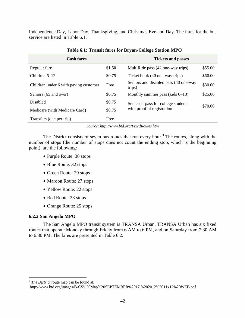
42

Independence Day, Labor Day, Thanksgiving, and Christmas Eve and Day. The fares for the bus service are listed in Table 6.1.

Table 6.1: Transit fares for Bryan-College Station MPO

Cash fares Tickets and passes

Regular fare $1.50 MultiRide pass (42 one-way trips) $55.00

Children 6–12 $0.75 Ticket book (40 one-way trips) $60.00

Children under 6 with paying customer Free Seniors and disabled pass (40 one-way trips)

$30.00

Seniors (65 and over) $0.75 Monthly summer pass (kids 6–18) $25.00

Disabled $0.75 Semester pass for college students with proof of registration

$70.00 Medicare (with Medicare Card) $0.75

Transfers (one per trip) Free

Source: http://www.btd.org/FixedRoutes.htm

The District consists of seven bus routes that run every hour.3 The routes, along with the number of stops (the number of stops does not count the ending stop, which is the beginning point), are the following:

• Purple Route: 38 stops

• Blue Route: 32 stops

• Green Route: 29 stops

• Maroon Route: 27 stops

• Yellow Route: 22 stops

• Red Route: 28 stops

• Orange Route: 25 stops

6.2.2 San Angelo MPO

The San Angelo MPO transit system is TRANSA Urban. TRANSA Urban has six fixed routes that operate Monday through Friday from 6 AM to 6 PM, and on Saturday from 7:30 AM to 6:30 PM. The fares are presented in Table 6.2.

3 The District route map can be found at: http://www.btd.org/images/B-CS%20Map%20SEPTEMBER%2017,%202012%2011x17%20WEB.pdf

43

Table 6.2: Transit fares for San Angelo MPO

Passenger Cash fare

Daily fare

Weekly fare

Monthly fare

Regular fare $2.00 $2.00 $10.00 $30.00

Seniors (60+), students, military, or disabled

$1.00 $1.00 $5.00 $15.00

Children 5 and under (must be accompanied by fare paying adult)

Free

Source: http://www.cvcog.org/cvcog/trans_urban.html

The six routes of TRANSA Urban, along with the number of stops, are the following:4

• Route 1: 12 stops





• Route 6–Goodfellow Express: 12 stops (only runs on Friday from 18:00 to 01:00 and Saturday 12:00 to 01:00).

6.2.3 Longview MPO

The Longview Transit system consists of seven fixed routes with fixed stops. However, travelers can also “wave down” a bus at any point on the route to board. The buses operate Monday through Friday from 6:15 AM to 7:15 PM, and on Saturdays from 7:15 AM to 7:15 PM. There is no service on Sundays. In addition, no service is provided on the following holidays: New Year’s Day, Memorial Day, Independence Day, Labor Day, Thanksgiving Day, and Christmas Day (although for these last two holidays, service may end early the day before). The transit fares are presented in Table 6.3.

Table 6.3: Transit fares for Longview MPO


Regular fare $1.25 Five tickets $6.25

Day pass $3.00 Ten tickets $12.50

Children (age 6 to 14 years) $0.65 Twenty tickets $25.00

Children under 6 years Free 31-day monthly pass $40.00

Students (ID required) $0.65 Student semester $100.00

Medicare, senior, disabled $0.60

Source: http://www.longviewtransit.com/ticket.php

4 TRANSA Urban route map is available at: http://media.gosanangelo.com/media/static/New_Bus_Schedule_for_web.pdf

44

Longview Transit’s routes and number of official stops are the following:5

• 1-Mobberly/LeTourneau Univ.: 5 stops

• 2-Medical District/Longview HS: 4 stops

• 3-Pine Tree/Springhill: 6 stops

• 4-East Marshall/Alpine: 4 stops

• 5-Loop 281/Silver Falls: 6 stops

• 6-MLK/South Eastman: 5 stops

• 7-Hwy 80 West/Gladewater (Newest Route: Monday-Friday only): 4 stops

6.2.4 Lubbock MPO

The Lubbock MPO public transit system is called Citibus. There are nine fixed routes throughout Lubbock, as well as numerous campus routes to/around Texas Tech. Citibus operates from 5:25 AM to 7:45 PM, Monday to Friday. On Saturday, the service begins at 6:45 AM and ends at 7:55 PM, and there is no service on Sunday. Citibus does not provide service on the following holidays: New Year’s Day, Memorial Day, Independence Day, Labor Day, Thanksgiving Day, and Christmas Day (Table 6.4).

Table 6.4: Transit fares for Lubbock MPO


Regular fare $1.75 One-day pass $3.50

Children (age 6 to 14 yrs) $1.25 Weekly pass $14.50

Children under 6 yrs Free Monthly pass $50.00

Medicare, seniors (65 yrs or older) and persons with disabilities

$0.85 One-day pass for Medicare, seniors (65 yrs or older) and persons with disabilities

$1.75

Weekly pass for Medicare, seniors (65 yrs or older) and persons with disabilities

$7.25

Monthly pass for Medicare, seniors (65 yrs or older) and persons with disabilities

$50.00

Source: http://www.citibus.com/page/services Citibus regular routes and number of stops are the following:6

• 1-Dunbar Area: 5 stops

• 2-East Broadway: 4 stops

• 5-Boston/S. Quaker/South Plains Mall: 6 stops

• 6-Buddy Holly/50th St. Crosstown: 5 stops

5 Longview Transit route maps can be found at: http://www.longviewtransit.com/routes.php 6 Citibus route maps are available at http://www.citibus.com/page/routes.

45

• 9-Ave. Q/S. University/S. Quaker: 5 stops

• 12-Arnett Benson/4th St.: 8 stops to/ 9 stops back

• 14-Cherry Point: 5 stops

• 19-Wayland Plaza/South Plains Mall: 7 stops

• 34-34th St./South Plains Mall: 6 stops

In addition, the following routes operate to/around Texas Tech.

• Texas Tech: 10 stops

• Red Raider: 10 stops

• Masked Rider: 7 Stops

• Overton Park North: 4 stops

• Overton Park South: 5 Stops

• Northwest: 6 stops

• North 4th: 8 stops

• North Indiana: 8 stops

• Tech Terrace: 10 Stops

• West 4th Express: 2 stops

• TTU s-Bus Safe Ride: 7 stops

6.3 Transit Skim Generation

The guidelines to generate the transit skims were discussed in Chapter 5. The first step towards developing the transit skims is to generate the transit network. Unfortunately, the metropolitan area networks were not available at this point of the project, and the only information the research team had are the network skims. Therefore, a different, and simpler, approach was used to generate the transit skims, as follows:

• In-vehicle travel time: IVTT was computed as a function of IVTT for drive-alone mode, as obtained from the network skims provided by TxDOT. In particular, IVTT for transit was assumed to be 25% higher than IVTT for auto for all TAZ pairs.

• Out-of-vehicle travel time: The access/egress time was defined as 3 minutes for all TAZ pairs, and the wait time was computed as half of the headway, based on the reported service frequencies. Finally, the OVVT is the sum of the access/egress time, plus the wait time.

• Cost: A flat cost was used for all TAZs pairs, equal to the regular fare.

• Number of transfers: considered to be zero for all TAZ pairs.

46


The estimation of mode choice models requires an accurate representation of the transportation system serving the region. In particular, the model estimation requires that the different skims are generated for each mode.

In the next chapter, we prepared data for mode choice estimation in one small-sized urban area and one medium-sized urban area, following the guidelines proposed earlier. In particular, for the network skims, we were able to obtain network data in order to then generate the transit network. The two urban areas that were employed in developing the model were a subset of the four considered in this chapter.

47

Chapter 7. Procedure to Prepare Data

The objective of this chapter is to provide the steps/procedures adopted in order to prepare the data for mode choice model estimation. Following the framework of Chapters 2 through 4, we focused exclusively on HB work trips. The research project required the CTR research team to develop a mode choice model for two Texas MPOs. We selected the Longview and Lubbock MPOs.

The selection is based on conversations with the PMC regarding survey data availability, and the recommendations made in Chapters 2 and 3. The MPOs’ locations are presented in Figure 7.1.

Figure 7.1: Selected study area

For each of the MPOs, we generated skims for five travel modes:

• Drive alone

• Carpool

• Transit (bus)

• Walk

• Bicycle

The remainder of the chapter is organized as follows. Section 7.1 provides information about the steps adopted in extracting necessary demographic data and trip characteristics from the survey data. Section 7.2 presents the steps and assumptions made in the development of skims for the two selected MPOs. Section 7.3 provides conclusions and recommendations where appropriate.

48

7.1 Procedure for Survey Data Extraction

The steps involved in extraction of demographic data and trip characteristics are identical for both the MPOs. This section discusses the steps involved for only one MPO, Lubbock (the same steps are assumed for the Longview MPO).

The mode choice survey data for both the MPOs was obtained from the Texas A&M Transportation Institute with the permission of TxDOT. The survey data consisted of following four files:

• Record Type 1, Household Information Data

• Record Type 2, Personal Information Data

• Record Type 3, Vehicle Information Data

• Record Type 4, Activity/Trip Data

Each of the four survey files contains a unique household number for each of the households. This unique household number is the key to finding information on households across different files.

The household information file contains information on household demographics, which includes household size, number of workers in the household, number of vehicles owned by household, household address, etc. The personal information file contains information about the individual such as gender, age, driver license status, employment status, etc. The vehicle information file contains information about the type of vehicle (car, van, motorcycle, etc.), make, model, year of manufacture, etc. The activity/trip file contains information on the purpose of the trip, trip origin and destination locations, mode of the trip, trip arrival and departure time, etc. The survey recorded all the trips made by an individual in the household on the day of the survey.

To develop a mode choice model, one can potentially include the whole range of demographic and trip characteristics in the model. However, in practice we include only the variables that are available/used in the Texas Package. We maintain this consistency to avoid any additional future data collection effort7. Hence, we include only household size and household income as demographic characteristics in the mode choice model development8. Further, from the activity data file, we obtain the purpose of the trip as the focus of the current work is HB work trips, mode of trip, and trip O-D in terms of a TAZ number. For ease in readability, Table 7.1 provides a list of variables whose extraction from survey data is required for the mode choice model estimation.

7 The mode choice model will be used to predict the mode share for the future year. Hence, including only the demographic variables available in the Texas Package ensures we will not need to collect additional data in upcoming years. 8 The Texas Package uses household size and household income as explanatory variable in the trip generation step and hence this data is available for each of the TAZ.

49

Table 7.1: List of demographic and trip variables

Demographic VariablesHousehold Size

Household Income

Trip Characteristics

Purpose of Trip

Mode of Trip

O-D of the Trip at TAZ Level

Given the list of variables required for the mode choice model estimation, we adopted the

following steps to extract the required variables from the survey data. We extracted the trip information for each of the households. This information includes

unique household number, person number (indicates the unique number of the person who participated in the survey), trip number, mode of trip, and purpose of the trip.

The determination of trip origin and destination is slightly complicated. In the survey data, the trip number is recorded as follows: The first trip for each person is recorded as zero for where their day began. Each subsequent trip is numbered sequentially 1, 2, 3, etc. Hence, the sequence of trips forms a chain starting with trip zero, and the previous trip location serves as an origin for the next trip. To avoid any mistake in recording O-D zone-pairs, we checked the arrival and departure time for each of the trips along with the trip number to ensure that proper ordering was maintained.

Once the trip characteristics were appended appropriately for each of the household members, we appended the demographic variables (household size and household income) for each of the individuals by matching the unique household number.

We also provide a list of alternatives available for mode of the trip, purpose of the trip, and household income in the survey data.

• Mode of the trip: It contains the following alternatives: Walk, Auto, Carpool, Vanpool, Commercial Vehicle, Bus, School Bus, Taxi, Bicycle, Motorcycle, and others.

• Purpose of the trip: It includes the following alternatives: Meal/Eat, Work-Related, School, Shopping, Personal (such as laundry or banking), Social/Recreation, and Pick up/Drop-off of Others.

• Household income: The household income was categorized into the following fifteen categories: less than $5,000, $5,000 to $9,999, $10,000 to $14,999, $15,000 to $19,999, $20,000 to $24,999, $25,000 to $29,999, $30,000 to $34,999, $35,000 to $39,999, $40,000 to $49,999, $50,000 to $59,999, $60,000 to $74,999, $75,000 to $99,999, $100,000 to $124,999, $125,000 to $149,999, and $150,000 or more.

Table 7.2 shows the mode share for both of the MPOs for the alternatives drive alone,

carpool, transit, walk, and bike9.

9 Since we report only the trips corresponding to HB trip purpose and five modes, the total sample size and frequency for each of the modes reported here will differ from the total survey sample size and corresponding mode frequencies.

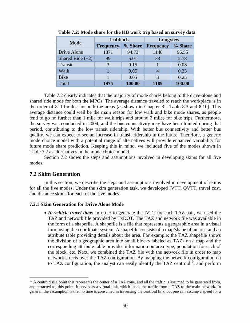
50

Table 7.2: Mode share for the HB work trip based on survey data

Table 7.2 clearly indicates that the majority of mode shares belong to the drive-alone and shared ride mode for both the MPOs. The average distance traveled to reach the workplace is in the order of 8–10 miles for both the areas (as shown in Chapter 8’s Table 8.3 and 8.10). This average distance could well be the main reason for low walk and bike mode shares, as people tend to go no further than 1 mile for walk trips and around 3 miles for bike trips. Furthermore, the survey was conducted in 2004, and the bus connectivity may have been limited during that period, contributing to the low transit ridership. With better bus connectivity and better bus quality, we can expect to see an increase in transit ridership in the future. Therefore, a generic mode choice model with a potential range of alternatives will provide enhanced variability for future mode share prediction. Keeping this in mind, we included five of the modes shown in Table 7.2 as alternatives in the mode choice model.

Section 7.2 shows the steps and assumptions involved in developing skims for all five modes.

7.2 Skim Generation

In this section, we describe the steps and assumptions involved in development of skims for all the five modes. Under the skim generation task, we developed IVTT, OVTT, travel cost, and distance skims for each of the five modes.

7.2.1 Skim Generation for Drive Alone Mode

• In-vehicle travel time: In order to generate the IVTT for each TAZ pair, we used the TAZ and network file provided by TxDOT. The TAZ and network file was available in the form of a shapefile. A shapefile is a file that represents a geographic area in a visual form using the coordinate system. A shapefile consists of a map/shape of an area and an attribute table providing details about the area. For example: the TAZ shapefile shows the division of a geographic area into small blocks labeled as TAZs on a map and the corresponding attribute table provides information on area type, population for each of the block, etc. Next, we combined the TAZ file with the network file in order to map network streets over the TAZ configuration. By mapping the network configuration on to TAZ configuration, the analyst can easily identify the TAZ centroid10, and perform

10 A centroid is a point that represents the center of a TAZ zone, and all the traffic is assumed to be generated from, and attracted to, this point. It serves as a virtual link, which loads the traffic from a TAZ to the main network. In general, the assumption is that no time is consumed in traversing the centroid link, but one can assume a speed for a

Mode Lubbock Longview

Frequency % Share Frequency % Share Drive Alone 1871 94.73 1148 96.55 Shared Ride (+2) 99 5.01 33 2.78 Transit 3 0.15 1 0.08 Walk 1 0.05 4 0.33 Bike 1 0.05 3 0.25 Total 1975 100.00 1189 100.00

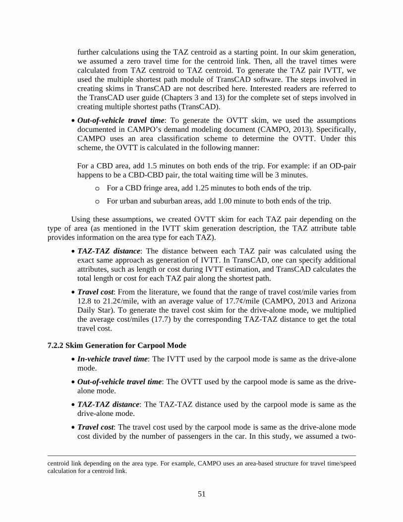
51

further calculations using the TAZ centroid as a starting point. In our skim generation, we assumed a zero travel time for the centroid link. Then, all the travel times were calculated from TAZ centroid to TAZ centroid. To generate the TAZ pair IVTT, we used the multiple shortest path module of TransCAD software. The steps involved in creating skims in TransCAD are not described here. Interested readers are referred to the TransCAD user guide (Chapters 3 and 13) for the complete set of steps involved in creating multiple shortest paths (TransCAD).

• Out-of-vehicle travel time: To generate the OVTT skim, we used the assumptions documented in CAMPO’s demand modeling document (CAMPO, 2013). Specifically, CAMPO uses an area classification scheme to determine the OVTT. Under this scheme, the OVTT is calculated in the following manner: For a CBD area, add 1.5 minutes on both ends of the trip. For example: if an OD-pair happens to be a CBD-CBD pair, the total waiting time will be 3 minutes.

o For a CBD fringe area, add 1.25 minutes to both ends of the trip.

o For urban and suburban areas, add 1.00 minute to both ends of the trip.

Using these assumptions, we created OVTT skim for each TAZ pair depending on the type of area (as mentioned in the IVTT skim generation description, the TAZ attribute table provides information on the area type for each TAZ).

• TAZ-TAZ distance: The distance between each TAZ pair was calculated using the exact same approach as generation of IVTT. In TransCAD, one can specify additional attributes, such as length or cost during IVTT estimation, and TransCAD calculates the total length or cost for each TAZ pair along the shortest path.

• Travel cost: From the literature, we found that the range of travel cost/mile varies from 12.8 to 21.2¢/mile, with an average value of 17.7¢/mile (CAMPO, 2013 and Arizona Daily Star). To generate the travel cost skim for the drive-alone mode, we multiplied the average cost/miles (17.7) by the corresponding TAZ-TAZ distance to get the total travel cost.

7.2.2 Skim Generation for Carpool Mode

• In-vehicle travel time: The IVTT used by the carpool mode is same as the drive-alone mode.

• Out-of-vehicle travel time: The OVTT used by the carpool mode is same as the drive-alone mode.

• TAZ-TAZ distance: The TAZ-TAZ distance used by the carpool mode is same as the drive-alone mode.

• Travel cost: The travel cost used by the carpool mode is same as the drive-alone mode cost divided by the number of passengers in the car. In this study, we assumed a two-

centroid link depending on the area type. For example, CAMPO uses an area-based structure for travel time/speed calculation for a centroid link.

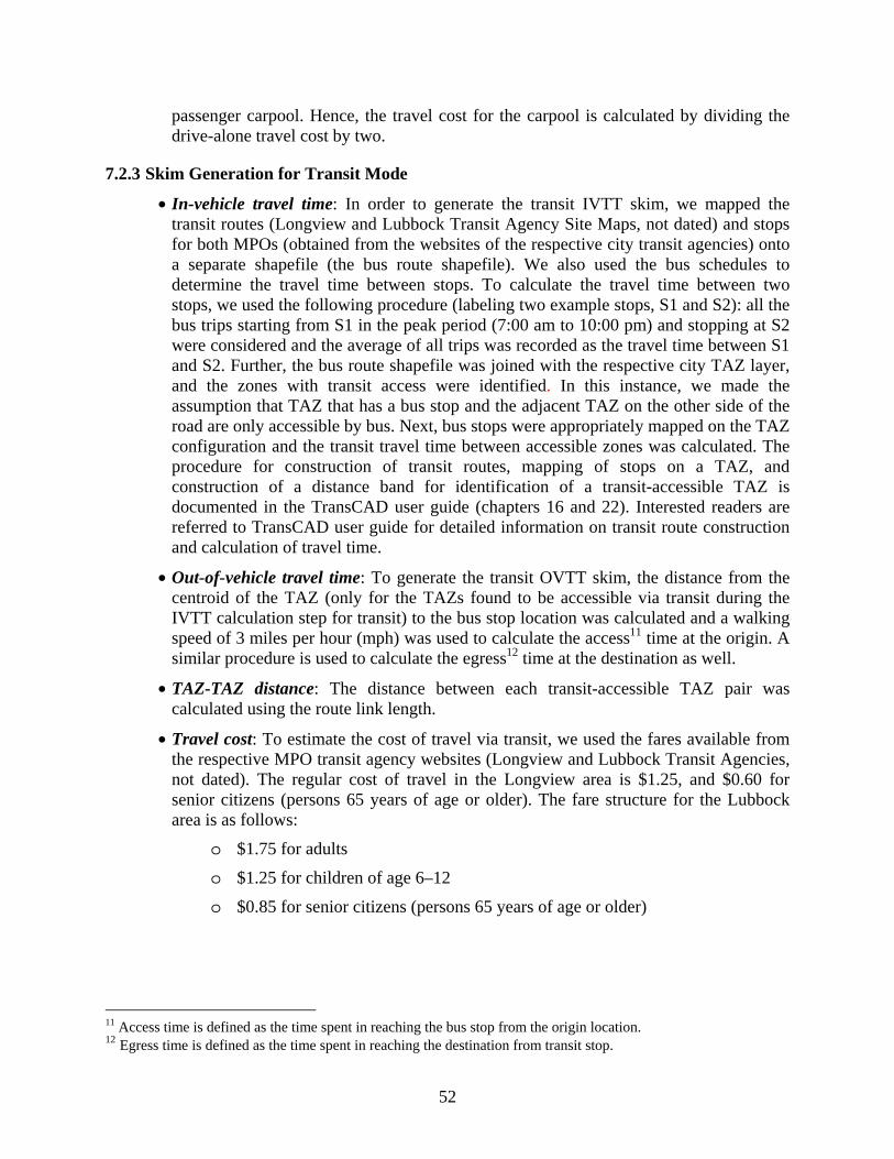
52

passenger carpool. Hence, the travel cost for the carpool is calculated by dividing the drive-alone travel cost by two.

7.2.3 Skim Generation for Transit Mode

• In-vehicle travel time: In order to generate the transit IVTT skim, we mapped the transit routes (Longview and Lubbock Transit Agency Site Maps, not dated) and stops for both MPOs (obtained from the websites of the respective city transit agencies) onto a separate shapefile (the bus route shapefile). We also used the bus schedules to determine the travel time between stops. To calculate the travel time between two stops, we used the following procedure (labeling two example stops, S1 and S2): all the bus trips starting from S1 in the peak period (7:00 am to 10:00 pm) and stopping at S2 were considered and the average of all trips was recorded as the travel time between S1 and S2. Further, the bus route shapefile was joined with the respective city TAZ layer, and the zones with transit access were identified. In this instance, we made the assumption that TAZ that has a bus stop and the adjacent TAZ on the other side of the road are only accessible by bus. Next, bus stops were appropriately mapped on the TAZ configuration and the transit travel time between accessible zones was calculated. The procedure for construction of transit routes, mapping of stops on a TAZ, and construction of a distance band for identification of a transit-accessible TAZ is documented in the TransCAD user guide (chapters 16 and 22). Interested readers are referred to TransCAD user guide for detailed information on transit route construction and calculation of travel time.

• Out-of-vehicle travel time: To generate the transit OVTT skim, the distance from the centroid of the TAZ (only for the TAZs found to be accessible via transit during the IVTT calculation step for transit) to the bus stop location was calculated and a walking speed of 3 miles per hour (mph) was used to calculate the access11 time at the origin. A similar procedure is used to calculate the egress12 time at the destination as well.

• TAZ-TAZ distance: The distance between each transit-accessible TAZ pair was calculated using the route link length.

• Travel cost: To estimate the cost of travel via transit, we used the fares available from the respective MPO transit agency websites (Longview and Lubbock Transit Agencies, not dated). The regular cost of travel in the Longview area is $1.25, and $0.60 for senior citizens (persons 65 years of age or older). The fare structure for the Lubbock area is as follows:

o $1.75 for adults

o $1.25 for children of age 6–12

o $0.85 for senior citizens (persons 65 years of age or older)

11 Access time is defined as the time spent in reaching the bus stop from the origin location. 12 Egress time is defined as the time spent in reaching the destination from transit stop.

53

7.2.4 Skim Generation for Walk Mode

• Walk time: To calculate the walk time between TAZ pairs, we assume an average walking speed of 3 mph. Then we calculated the shortest path between each TAZ pair in terms of distance by constraining the highway segments. Here we assumed that people tend to avoid highway segments when using the walk trip mode for commuting. Next, we divided the zone pair distances by the average walking speed to obtain the TAZ walk travel time skim.

• TAZ-TAZ distance: Here, we use the distance configuration matrix obtained during the walk time skim generation for the walk mode.

7.2.5 Skim Generation for Bike Mode

• Out-of-vehicle travel time: To generate the OVTT skim for the bike mode, we assumed an average bike speed of 11 mph. We found that CAMPO (Lubbock Avalanche Journal, not dated) uses a speed range of 10–12 mph for the bike mode. Similar to the walk mode calculation, we assumed that people do not use highway segments while using a bike in a commute mode. Hence, we use the same TAZ distance configuration matrix obtained for the walk mode and divided the distances by average bike speed (11 mph) to obtain the bike travel time skim.

• TAZ-TAZ distance: Here, we use the distance configuration matrix obtained during OVTT skim generation for the bike mode.


The estimation of mode choice models requires information on an individual’s demographic and trip characteristics. Demographic data and a certain set of trip characteristics, such as the mode of travel, purpose of travel, location of travel, etc., are available from the survey data. However, data on other trip characteristics, known as skims, are generally not available from the survey and need to be constructed for each of the travel modes considered in the analysis. In this chapter we extracted the required set of demographic variables and trip characteristics from the survey data for the Longview and Lubbock MPOs. Further, we also constructed the IVTT skim, OVTT skim, travel distance skim, and travel cost skim for both MPOs using the guidelines developed in Chapters 4 through 6. We documented any assumptions made during construction of a skim. All the assumptions were made after referring to other MPOs’ TDMs and skim generation guidelines/assumptions to obtain consistent estimates.

In Chapter 8 we will estimate the MNL and NL model for both MPOs using the data prepared in Chapter 7. Further, the estimated model coefficients will be used to develop an Excel-based forecasting tool for mode choice at the TAZ level, which will be discussed in Chapter 8.

55

Chapter 8. Model Development

8.1 Introduction and Overview

This chapter describes the mode choice model for two medium/small-sized MPOs: Lubbock and Longview. The need for the addition of a mode choice model to the four-step planning process for medium/small-sized MPOs is evident: all 21 small and medium MPOs in Texas plan to improve their public transportation systems, incentivize non-motorized modes, reduce emissions, and provide more multi-model transportation options by year 2035 as a part of their strategic planning goals. To evaluate the impact of such policies, all the MPOs will require a mode choice model—but currently, none of the medium to small MPOs has a mode choice model in their four-step planning process.

The mode choice model developed here is for HB work trips exclusively; the data for the model development is derived from a 2005 survey.

8.2 Lubbock MPO

8.2.1 Traffic Analysis Zones

The Lubbock area has 723 internal TAZs. Each TAZ is classified into one of four area types: CBD, CBD fringe, urban, and suburban.

8.2.2 Modes

In the current model development, we considered five modes: drive alone, shared ride, transit, walk, and bike.

8.2.3 Network and Level-of-Service Preparation

The level-of-service variables (IVTT and OVTT, travel cost, and travel distance) were generated for all five modes considered in the analysis. The network file obtained from TxDOT forms the basis for development of level-of-service variables for all but transit mode. The IVTT and travel distance for the drive-alone and shared ride modes were determined by running multiple shortest paths in TransCAD. To obtain the travel cost for the drive-alone and shared ride modes, a per-mile gasoline cost of $0.25 was assumed. A skim development guide is provided in Appendix A detailing all the steps involved in the development of level-of-service variables for the five modes in TransCAD and ArcMap. In a similar fashion, the travel distance and OVTT for walk and bike mode was developed given certain assumptions (i.e., people tend to avoid freeways and highways when using the walk and bike mode to commute and the average walking and biking speeds are, respectively, 3 mph and 11 mph). The level-of-service variables for the transit mode were developed using the transit network obtained from the transit operator’s website. The transit fare was also obtained from the transit operator’s website. For the Lubbock area, the fare is $1.75 for the general public. We would like to point out that the transit network obtained from transit operators website was not a geographical file but a simple digital image. The process of creating a geographical file from a digital image is complex, and thus it is not described in this chapter; see the skim development guide in Appendix A.

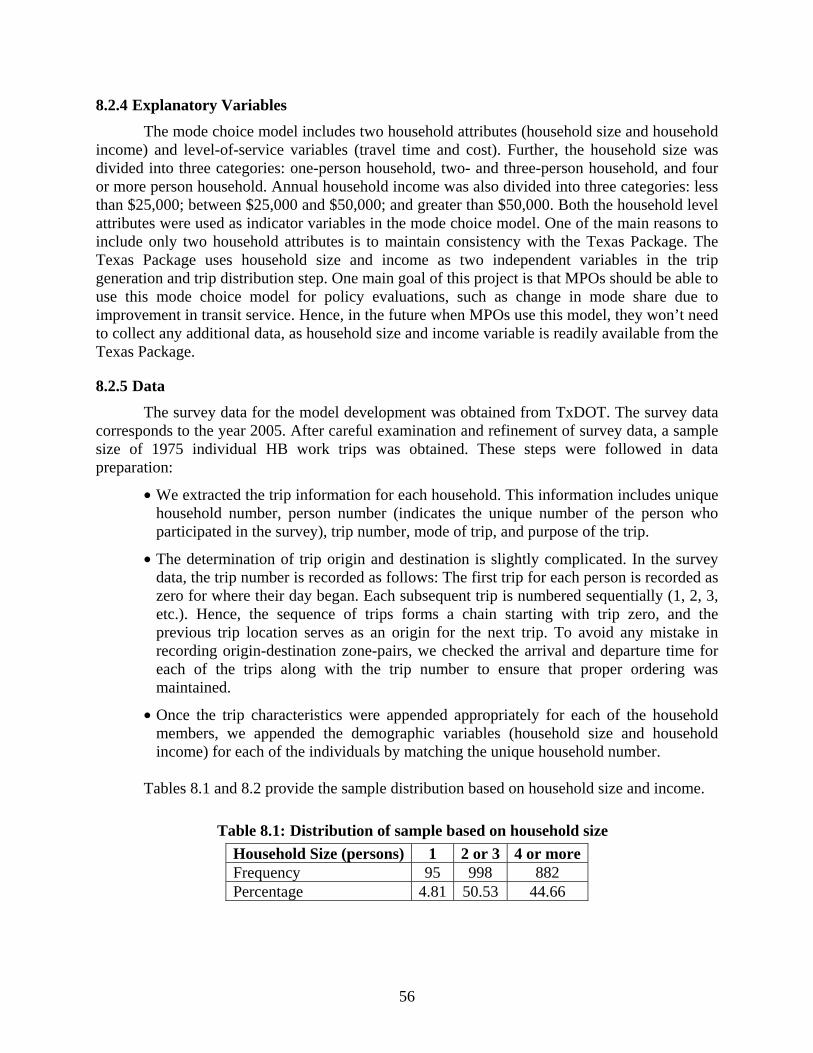
56

8.2.4 Explanatory Variables

The mode choice model includes two household attributes (household size and household income) and level-of-service variables (travel time and cost). Further, the household size was divided into three categories: one-person household, two- and three-person household, and four or more person household. Annual household income was also divided into three categories: less than $25,000; between $25,000 and $50,000; and greater than $50,000. Both the household level attributes were used as indicator variables in the mode choice model. One of the main reasons to include only two household attributes is to maintain consistency with the Texas Package. The Texas Package uses household size and income as two independent variables in the trip generation and trip distribution step. One main goal of this project is that MPOs should be able to use this mode choice model for policy evaluations, such as change in mode share due to improvement in transit service. Hence, in the future when MPOs use this model, they won’t need to collect any additional data, as household size and income variable is readily available from the Texas Package.

8.2.5 Data The survey data for the model development was obtained from TxDOT. The survey data

corresponds to the year 2005. After careful examination and refinement of survey data, a sample size of 1975 individual HB work trips was obtained. These steps were followed in data preparation:

• We extracted the trip information for each household. This information includes unique household number, person number (indicates the unique number of the person who participated in the survey), trip number, mode of trip, and purpose of the trip.

• The determination of trip origin and destination is slightly complicated. In the survey data, the trip number is recorded as follows: The first trip for each person is recorded as zero for where their day began. Each subsequent trip is numbered sequentially (1, 2, 3, etc.). Hence, the sequence of trips forms a chain starting with trip zero, and the previous trip location serves as an origin for the next trip. To avoid any mistake in recording origin-destination zone-pairs, we checked the arrival and departure time for each of the trips along with the trip number to ensure that proper ordering was maintained.

• Once the trip characteristics were appended appropriately for each of the household members, we appended the demographic variables (household size and household income) for each of the individuals by matching the unique household number.

Tables 8.1 and 8.2 provide the sample distribution based on household size and income.

Table 8.1: Distribution of sample based on household size

Household Size (persons) 1 2 or 3 4 or more Frequency 95 998 882 Percentage 4.81 50.53 44.66

57

Table 8.2: Distribution of sample based on household income

Income Frequency PercentageLess than 25K 236 11.95 Between 25K & 50K 585 29.62 Greater than 50K 1154 58.43

Table 8.1 indicates that the majority of the population is distributed among household

sizes of “two or three” and “four or more.” We may infer from Table 8.1 that most of the households are married couples with one or more children. Similarly, Table 8.2 appears to indicate that the majority of the population is in the high income category (greater than $50,000).

Table 8.3 provides the descriptive statistics for level-of-service variables for all five modes.

Table 8.3: Descriptive statistics for level-of-service variable

Variables Minimum Maximum AverageStandard Deviation

Frequency

IVTT for DA & SR+2 (Min)*

0.1 59.9 14.1 10.4 1975

OVTT for DA & SR+2 (Min)

2 2.8 2.3 0.2 1975

Travel Distance for DA & SR+2 (Miles)

0.1 47.1 10.1 8.2 1975

Travel Cost for DA (Dollars)

0.01 11.8 2.5 2.1 1975

Travel Cost for SR+2 (Dollars)

0.01 5.9 1.3 1 1975

IVTT for Transit (Min) 4.0 25.0 9.2 4 54 OVTT for Transit (Min) 3.9 18.4 10.3 2.7 54 Travel Cost for Transit (Dollars)

1.8 1.8 1.8 0 54

Trip time for Walk (Min) 29.8 19.6 7.8 0.3 81 Trip Distance for Walk (Miles)

1.5 1 0.4 0.1 81

Trip time for Bike (Min) 0.3 40 23.1 9.8 997 Trip Distance for Bike (Miles)

0.1 7.3 4.2 1.8 997

DA = drive alone; SR = shared ride For each level-of-service variable, we report the minimum, maximum, average, standard

deviation, and frequency. The column frequency indicates the number of samples for which the corresponding mode is available. In order to obtain the availability of walk and bike modes, a maximum limit of 30 minutes on walking and 40 minutes on biking was imposed and then trips were appropriately assigned the walk and bike mode availability. An important point to note here is that only 54 observations/trips have accessibility to transit. The transit availability was determined using the condition that both origin and destination TAZs were accessible to transit

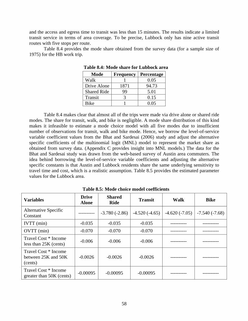
58

and the access and egress time to transit was less than 15 minutes. The results indicate a limited transit service in terms of area coverage. To be precise, Lubbock only has nine active transit routes with five stops per route.

Table 8.4 provides the mode share obtained from the survey data (for a sample size of 1975) for the HB work trip.

Table 8.4: Mode share for Lubbock area

Mode Frequency PercentageWalk 1 0.05 Drive Alone 1871 94.73 Shared Ride 99 5.01 Transit 3 0.15 Bike 1 0.05

Table 8.4 makes clear that almost all of the trips were made via drive alone or shared ride

modes. The share for transit, walk, and bike is negligible. A mode share distribution of this kind makes it infeasible to estimate a mode choice model with all five modes due to insufficient number of observations for transit, walk and bike mode. Hence, we borrow the level-of-service variable coefficient values from the Bhat and Sardesai (2006) study and adjust the alternative specific coefficients of the multinomial logit (MNL) model to represent the market share as obtained from survey data. (Appendix C provides insight into MNL models.) The data for the Bhat and Sardesai study was drawn from the web-based survey of Austin area commuters. The idea behind borrowing the level-of-service variable coefficients and adjusting the alternative specific constants is that Austin and Lubbock residents share the same underlying sensitivity to travel time and cost, which is a realistic assumption. Table 8.5 provides the estimated parameter values for the Lubbock area.

Table 8.5: Mode choice model coefficients

Variables Drive Alone

Shared Ride

Transit Walk Bike

Alternative Specific Constant

---------- -3.780 (-2.86) -4.520 (-4.65) -4.620 (-7.05) -7.540 (-7.68)

IVTT (min) -0.035 -0.035 -0.035 ---------- ----------

OVTT (min) -0.070 -0.070 -0.070 ---------- ----------

Travel Cost * Income less than 25K (cents)

-0.006 -0.006 -0.006 ---------- ----------

Travel Cost * Income between 25K and 50K (cents)

-0.0026 -0.0026 -0.0026 ---------- ----------

Travel Cost * Income greater than 50K (cents)

-0.00095 -0.00095 -0.00095 ---------- ----------

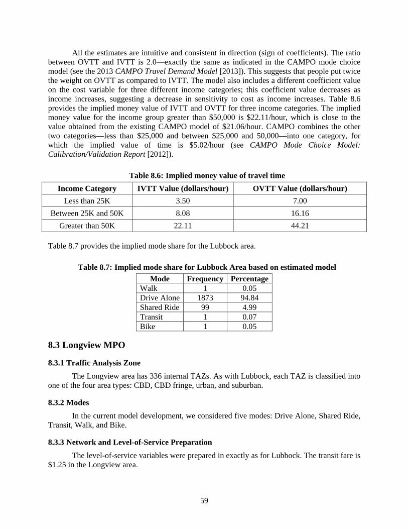
59

All the estimates are intuitive and consistent in direction (sign of coefficients). The ratio between OVTT and IVTT is 2.0—exactly the same as indicated in the CAMPO mode choice model (see the 2013 CAMPO Travel Demand Model [2013]). This suggests that people put twice the weight on OVTT as compared to IVTT. The model also includes a different coefficient value on the cost variable for three different income categories; this coefficient value decreases as income increases, suggesting a decrease in sensitivity to cost as income increases. Table 8.6 provides the implied money value of IVTT and OVTT for three income categories. The implied money value for the income group greater than $50,000 is $22.11/hour, which is close to the value obtained from the existing CAMPO model of $21.06/hour. CAMPO combines the other two categories—less than $25,000 and between $25,000 and 50,000—into one category, for which the implied value of time is $5.02/hour (see CAMPO Mode Choice Model: Calibration/Validation Report [2012]).

Table 8.6: Implied money value of travel time

Income Category IVTT Value (dollars/hour) OVTT Value (dollars/hour)

Less than 25K 3.50 7.00

Between 25K and 50K 8.08 16.16

Greater than 50K 22.11 44.21

Table 8.7 provides the implied mode share for the Lubbock area.

Table 8.7: Implied mode share for Lubbock Area based on estimated model


8.3 Longview MPO

8.3.1 Traffic Analysis Zone

The Longview area has 336 internal TAZs. As with Lubbock, each TAZ is classified into one of the four area types: CBD, CBD fringe, urban, and suburban.

8.3.2 Modes In the current model development, we considered five modes: Drive Alone, Shared Ride,

Transit, Walk, and Bike.

8.3.3 Network and Level-of-Service Preparation The level-of-service variables were prepared in exactly as for Lubbock. The transit fare is

$1.25 in the Longview area.

60

8.3.4 Explanatory Variables The same configuration of explanatory variables was used for Longview as for Lubbock.

8.3.5 Data The survey data for the model development was obtained from TxDOT. The survey data

corresponds to the year 2005. After careful examination and refinement of survey data, a sample size of 1189 individual HB work trips was prepared. The data preparation steps are same as discussed for Lubbock area. Tables 8.8 and 8.9 provide the sample distribution based on household size and income.

Table 8.8: Distribution of sample based on household size

Household Size (persons) 1 2 or 3 4 or more Frequency 67 692 430 Percentage 5.63 58.20 36.16

Table 8.9: Distribution of sample based on household income

Income Frequency PercentageLess than 25K 124 10.43 Between 25K & 50K 417 35.07 Greater than 50K 648 54.50

Table 8.8 clearly indicates that a majority of the population is has a household size of

“two or three.” We may infer from Table 8.8 that most of the households are married couples with one or more children. Similarly, Table 8.9 appears to indicate that the majority of the population is in the high income category (greater than $50,000).

In Table 8.10, we provide the descriptive statistics for level-of-service variables for all five modes.

61

Table 8.10: Descriptive statistics for level-of-service variable

Variables Minimum Maximum AverageStandard Deviation

Frequency

IVTT for DA & SR (Min)* 0.4 58.2 13.1 8.5 1189 OVTT for DA & SR (Min) 2.0 2.8 2.1 0.2 1189 Travel Distance for DA & SR (Miles)

0.2 35.7 8.2 5.7 1189

Travel Cost for DA (Dollars)

0.1 8.9 2.0 1.4 1189

Travel Cost for SR (Dollars) 0.1 4.5 1.0 0.7 1189 IVTT for Transit (Min) 5.0 25.0 9.7 4.9 15 OVTT for Transit (Min) 7.8 18.3 14.7 3.3 15 Travel Cost for Transit (Dollars)

1.3 1.3 1.3 0 15

Trip time for Walk (Min) 3.8 29.2 21.4 5.8 66 Trip Distance for Walk (Miles)

0.2 1.5 1.1 0.3 66

Trip time for Bike (Min) 1 40 22.2 9.8 671 Trip Distance for Bike (Miles)

0.2 7.3 4.1 1.8 671

DA = drive alone; SR = shared ride

The walk and bike mode availability was determined using the same conditions as in the Longview area. An important point to note here is that once again only 15 observations/trips have accessibility to transit, indicating a limited transit service in terms of area coverage. To be precise, Longview has only five active transit routes with five stops per route.

Table 8.11 provides the mode share obtained from the survey data (for a sample size of 1189) for the HB work trips.

Table 8.11: Mode share for Longview area


Table 8.11 demonstrates that, as in Lubbock, almost all of the trips were made via the

drive alone or shared ride mode. The share for transit, walk, and bike is negligible. A mode share distribution of this kind makes it infeasible to estimate a mode choice model with all five modes, due to an insufficient number of observations for transit, walk, and bike modes. Hence, we borrow the level-of-service variable coefficient values from the Bhat and Sardesai (2006) study and adjust the alternative specific coefficients of the MNL model to represent the market share as obtained from survey data, as was done for Lubbock area. Table 8.12 provides the estimated

62

parameter values for the Longview area—values that are highly similar to those in Table 8.5 for Longview.

Table 8.12: Mode choice model coefficients

Variables Drive Alone

Shared Ride

Transit Walk Bike

Alternative Specific Constant

---------- -3.20 (-1.85) -3.00 (-5.65) -4.75 (-5.36) -6.05 (-10.51)

IVTT (min) -0.035 -0.035 -0.035 ---------- ----------

OVTT (min) -0.070 -0.070 -0.070 ---------- ----------

Travel Cost * Income less than 25K (cents)

-0.006 -0.006 -0.006 ---------- ----------

Travel Cost * Income between 25K and 50K (cents)

-0.0026 -0.0026 -0.0026 ---------- ----------

Travel Cost * Income greater than 50K (cents)

-0.00095 -0.00095 -0.00095 ---------- ----------

Finally, Table 8.13 provides the implied mode share for the Longview area.

Table 8.13: Implied mode share for Longview area based on estimated model


63

Chapter 9. Conclusions

This project focuses on developing a process and a framework for (1) generating the inputs needed for estimating a travel mode choice model that includes the transit mode, and (2) developing a framework for implementing the results of an estimated travel mode choice model to project mode shares in response to demographic changes and to improvements in transit service.

In terms of generating the inputs for estimating a mode choice model, an important component is the generation of the necessary network skims (travel times and costs) by alternative modes. Most metropolitan planning organizations (MPOs) have good geographic information systems (GIS)-based representations of the highway network, which can be used to generate drive-alone and shared-ride skims (based on certain assumptions, as discussed in detail in Chapter 8). However, this is not the case with transit skims because of the lack of a good GIS-based representation of the transit network. Even in cases where a GIS-based transit (bus) network representation of stops is available, our experience has been that these stops are not locationally consistent with the highway link networks. In our project, we had to manually geo-code the bus stop information onto the highway network, and then make assumptions to generate transit paths and corresponding zone-to-zone transit skims. While we have provided a guidebook that provides a step-by-step procedure for doing so, a good georeferenced coordinate system— even just for stop locations—will substantially help in the transit skim generation process. In any case, MPOs should be prepared to expend about 4 weeks of time to develop a good representation of the transit network from which to develop transit skims.

The estimation of the mode choice model, given a set of trips and their characteristics, can be achieved using any standard software package. The database for this estimation may be developed using household survey data that provides information on trips, trip characteristics (origin and destination, from which the network skims can be created), and the characteristics of the individuals pursuing the trips. In this project, only two demographic variables were used in the mode choice model: household size and income. This approach was taken because the trip generation part of the Texas Package uses only these two demographic variables. Thus, person-trips may be generated in the Texas Package, and then taken through trip distribution, followed by a conversion from production-attractions to origin-destinations. The resulting traffic analysis zone (TAZ)-to-TAZ person-trips by household size category and income level category can be taken as input by the estimated mode choice model to determine modal shares (and thus zone-to-zone motorized vehicle trips).

The estimated models have been embedded into a software forecasting platform to predict modal share shifts between each pair of TAZs (and the region as a whole) arising in response to changes in income levels and/or household size over time. The models can also be used to assess the impacts of transit improvements (in terms of in-vehicle transit times as well as OVTTs, such as increasing the frequency of service). We should point out, however, that the model specifications embedded in the software platform need substantial improvement before actual implementation of the software—very few transit riders appeared in the household survey data sets used in estimation. This factor, in addition to the usual difficulty in disentangling time and cost effects from observed revealed preference data, led to a specification that has left very substantial room for improvement. For a trip-based mode choice model, one possibility to improve the specification is to use additional data from on-board transit surveys to increase the number of transit users in the mode choice estimation data set.

64

Four inter-related directions present themselves as potential avenues for implementation of this project’s results. The first is to examine transit skim development methods in more detail. In the current project, the skims were developed using several assumptions. An implementation project can examine the correctness of these assumptions and propose alternative assumptions where appropriate. It can also develop clear protocols and recommendations for procedures that MPOs can follow that will make the construction of these transit skims much easier. The second is to integrate the mode choice framework developed in this project into the current trip-based modeling system used by TxDOT’s Transportation Planning and Programming Division. The third is to pilot-implement the proposed modeling framework and approach in a few MPOs in the state, with the improved transit skim methods (also developed as part of an implementation) and better mode choice data (that also uses on-board transit survey data). The fourth is to provide workshops on the actual implementation of the mode choice model, integrated as part of the broader trip-based travel model system.

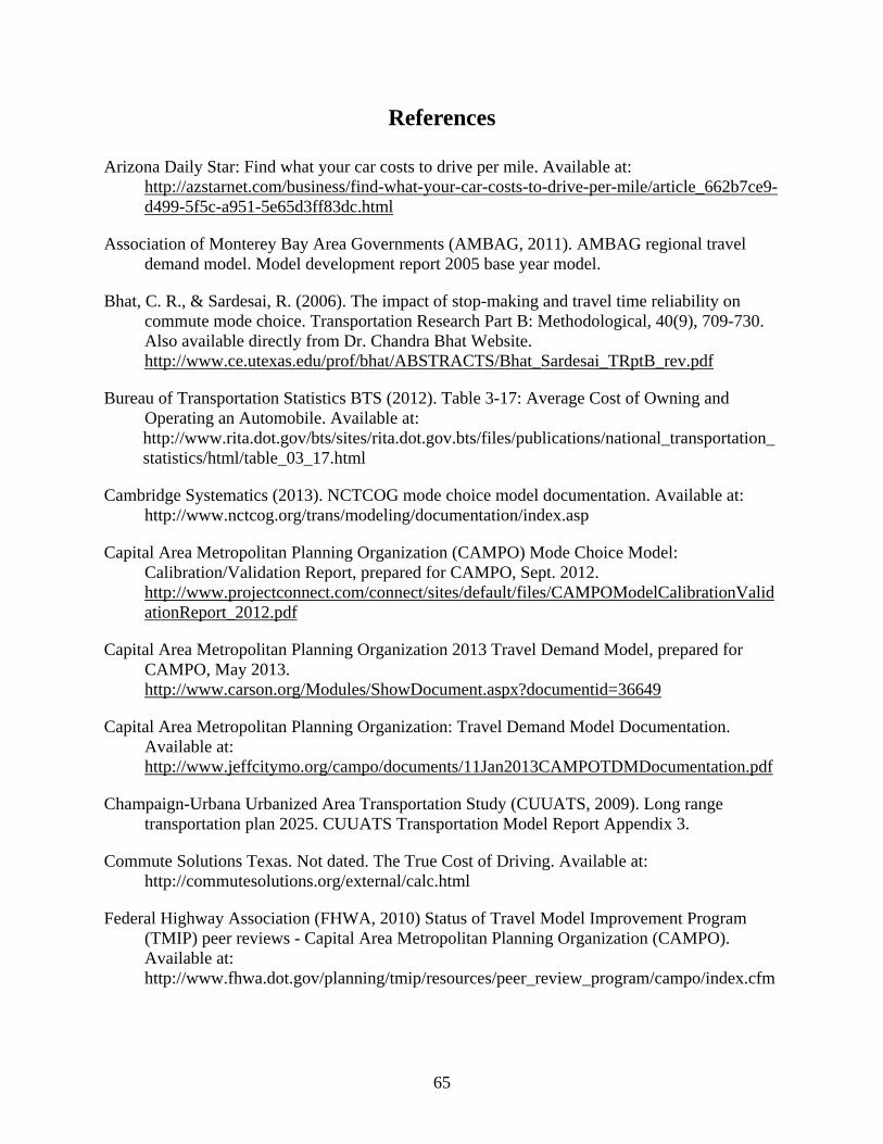
65

References

Arizona Daily Star: Find what your car costs to drive per mile. Available at: http://azstarnet.com/business/find-what-your-car-costs-to-drive-per-mile/article_662b7ce9-d499-5f5c-a951-5e65d3ff83dc.html

Association of Monterey Bay Area Governments (AMBAG, 2011). AMBAG regional travel demand model. Model development report 2005 base year model.

Bhat, C. R., & Sardesai, R. (2006). The impact of stop-making and travel time reliability on commute mode choice. Transportation Research Part B: Methodological, 40(9), 709-730. Also available directly from Dr. Chandra Bhat Website. http://www.ce.utexas.edu/prof/bhat/ABSTRACTS/Bhat_Sardesai_TRptB_rev.pdf

Bureau of Transportation Statistics BTS (2012). Table 3-17: Average Cost of Owning and Operating an Automobile. Available at: http://www.rita.dot.gov/bts/sites/rita.dot.gov.bts/files/publications/national_transportation_statistics/html/table_03_17.html

Cambridge Systematics (2013). NCTCOG mode choice model documentation. Available at: http://www.nctcog.org/trans/modeling/documentation/index.asp

Capital Area Metropolitan Planning Organization (CAMPO) Mode Choice Model: Calibration/Validation Report, prepared for CAMPO, Sept. 2012. http://www.projectconnect.com/connect/sites/default/files/CAMPOModelCalibrationValidationReport_2012.pdf

Capital Area Metropolitan Planning Organization 2013 Travel Demand Model, prepared for CAMPO, May 2013. http://www.carson.org/Modules/ShowDocument.aspx?documentid=36649

Capital Area Metropolitan Planning Organization: Travel Demand Model Documentation. Available at: http://www.jeffcitymo.org/campo/documents/11Jan2013CAMPOTDMDocumentation.pdf

Champaign-Urbana Urbanized Area Transportation Study (CUUATS, 2009). Long range transportation plan 2025. CUUATS Transportation Model Report Appendix 3.

Commute Solutions Texas. Not dated. The True Cost of Driving. Available at: http://commutesolutions.org/external/calc.html

Federal Highway Association (FHWA, 2010) Status of Travel Model Improvement Program (TMIP) peer reviews - Capital Area Metropolitan Planning Organization (CAMPO). Available at: http://www.fhwa.dot.gov/planning/tmip/resources/peer_review_program/campo/index.cfm

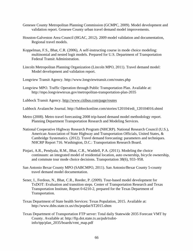
66

Genesee County Metropolitan Planning Commission (GCMPC, 2009). Model development and validation report. Genesee County urban travel demand model improvements.

Houston-Galveston Area Council (HGAC, 2012). 2009 model validation and documentation, Regional travel models.

Koppelman, F.S., Bhat, C.R. (2006), A self-instructing course in mode choice modeling: multinomial and nested logit models. Prepared for U.S. Department of Transportation Federal Transit Administration.

Lincoln Metropolitan Planning Organization (Lincoln MPO, 2011). Travel demand model: Model development and validation report.

Longview Transit Agency. http://www.longviewtransit.com/routes.php

Longview MPO. Traffic Operation through Public Transportation Plan. Available at: http://mpo.longviewtexas.gov/metropolitan-transportation-plan-2035

Lubbock Transit Agency. http://www.citibus.com/page/routes

Lubbock Avalanche Journal. http://lubbockonline.com/stories/120104/edi_120104016.shtml

Metro (2008). Metro travel forecasting 2008 trip-based demand model methodology report. Planning Department Transportation Research and Modeling Services.

National Cooperative Highway Research Program (NHCRP). National Research Council (U.S.), American Association of State Highway and Transportation Officials, United States, & Cambridge Systematics. (2012). Travel demand forecasting: parameters and techniques. NHCRP Report 716. Washington, D.C.: Transportation Research Board.

Pinjari, A.R., Pendyala, R.M., Bhat, C.R., Waddell, P.A. (2011). Modeling the choice continuum: an integrated model of residential location, auto ownership, bicycle ownership, and commute tour mode choice decisions. Transportation 38(6), 933–958.

San Antonio Bexar County MPO (SABCMPO, 2011). San Antonio/Bexar County 5-county travel demand model documentation.

Sener, I., Ferdous, N., Bhat, C.R., Reeder, P. (2009). Tour-based model development for TxDOT: Evaluation and transition steps. Center of Transportation Research and Texas Transportation Institute, Report 0-6210-2, prepared for the Texas Department of Transportation.

Texas Department of State health Services: Texas Population, 2015. Available at: http://www.dshs.state.tx.us/chs/popdat/ST2015.shtm

Texas Department of Transportation FTP server: Total daily Statewide 2035 Forecast VMT by County. Available at: http://ftp.dot.state.tx.us/pub/txdot-info/tpp/plan_2035/boards/vmt_map.pdf

67

Texas Department of Transportation FTP server: Texas Motor Vehicle Traffic Crash Highlights calendar Year 2012. Available at : http://ftp.dot.state.tx.us/pub/txdot-info/trf/crash_statistics/2012/01_2012.pdf

The snapshot of travel modeling activities: The state of Texas. Available at: http://media.tmiponline.org/clearinghouse/FHWA%E2%80%90HEP%E2%80%9012%E2%80%90005/Snapshot_of_Modeling_in_Texas.pdf

TransCAD, Transportation Planning Software User’s Guide, Caliper Corporation.

Texas State Data Center (2011). Descriptive tables - population, 2000–2010 total population by race/ethnicity. Available at: http://txsdc.utsa.edu/Reports/Subject/Population.aspx

U.S. Department of Commerce, United States Census Bureau: State & County Quick Facts, Texas. Available at: http://quickfacts.census.gov/qfd/states/48000.html

69

Appendix A. Guide to Model Skim Generation Development in TransCAD and ArcMap 10.1

Development of Skims for Drive Alone and Shared Ride

The development of skims refers to the process of developing the in-vehicle travel time, out-of-vehicle travel time, travel distance, and travel cost matrix for each traffic analysis zone (TAZ) pair for any given area. Skims are the required model input in any mode choice model, as they capture the traveler’s sensitivity to time (in-vehicle and out-of vehicle travel time), cost, and distance.

Required Input for Skim Development in TransCAD

To develop the skims for any ground-operated mode, the user needs two files:

• Coded street layer “network lines” with the following attributes: length, speed, travel time, one-way capacity, direction code, link type13, and any other link attribute.

• TAZ layer with the following attributes: TAZ type14, TAZ number, TAZ centroid node number, and any other information on the TAZ.

These two files should be available from the MPO in a TransCAD-compatible format.

Possible File Formats

To ensure compatibility with TransCAD, the files need to be in one of these two formats:

.cdf, .dbd: Indicates a file format directly compatible with TransCAD

.shp: Indicates a shapefile compatible with ArcGIS. If the required input files are available in the .cdf or .dbd format, the user is ready for the

next modeling steps. However, if the input files are available in the .shp format, the user needs to first convert them into the format required by TransCAD by performing the following steps:

• Open a session of TransCAD, and go to File->Open and point to the required folder.

• If you do not see your .shp file, change the file type to ESRI shapefile (*.shp) at the bottom of the window under the title “Files of type:” as shown in Figure A.1.

13 Link type refers to the functional classification of the roadway facility, such as state highway, freeway, arterial, etc. 14 TAZ type refers to the classification of an area into central business district, urban area, urban fringe, rural area, etc.

70

Figure A.1: File selection menu

• Select the file and click Open. It opens a window as shown in Figure A.2.

Figure A.2: Import shapefile window

• Check the Import Layer box and click OK.

• Upon clicking the OK button, TransCAD opens a window as shown in Figure A.3 and allows the user to save the file as a .dbd file. Provide a name and save the file into the .dbd format.

71

Figure A.3: File save menu

Creating the Overview Map

The first step in the skim development process is creation of the overview map by combining the network and TAZ files. To create the overview map, follow the steps in this section. Add the TAZ layer

• Choose File->Open and select the TAZ Geographic File (.dbd format) and click Open as shown in Figure A.4.

Figure A.4: Geographic file selection window

• To label the zones, click on the Automatic Labels button on the toolbar. TransCAD opens a window as shown in Figure A.5.

72

• Chose the field TAZ from the Field drop-down list. Adjust the font size and color as convenient and click OK. This will display the TAZ number at the center of each TAZ.

Figure A.5: TAZ visual setting window

Add the Network Layer and Node Layer

• Chose Map->Layers or click the button on the toolbar. TransCAD opens a window as shown in Figure A.6.

• Click on the Add Layer button. Select the Network file and click Open. This will add the Network file to the list of layers.

Figure A.6: Layer addition window

73

• Follow the same procedure and add the Node file to the layer list. Select Node layer and click on Hide Layer button. This will add the Node file to the layer list, but hide the nodes on the map (Figure A.7). If you wish to see the details of the Node file at any point in the modeling process, simply make the layer visible by selecting the Node layer and clicking on the Show Layer button as shown in Figure A.8.

Figure A.7: Layer visualization window

Figure A.8: Layer visualization window

• Click the Close button. At this moment, the TAZ boundaries and Network lines are not clearly visible.

Change the Zone and Network Style

• From the drop-down list of layers on the toolbar (shown in Figure A.9), choose the layer on which you want to modify the visual settings.

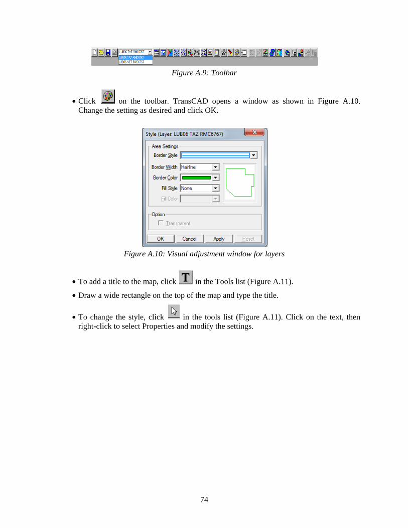
74

Figure A.9: Toolbar

• Click on the toolbar. TransCAD opens a window as shown in Figure A.10. Change the setting as desired and click OK.

Figure A.10: Visual adjustment window for layers

• To add a title to the map, click in the Tools list (Figure A.11).

• Draw a wide rectangle on the top of the map and type the title.

• To change the style, click in the tools list (Figure A.11). Click on the text, then right-click to select Properties and modify the settings.

75

Figure A.11: Tools ribbon

Save Your Work

• Chose File->Save or click on the toolbar. Provide the file name and click Save.

At this point, we have finished the overview map and are ready to begin the next step of skim development.

Creating the Centroid Set

• Select the Node Layer from the drop-down menu on the toolbar as shown in Figure A.12. If the Node layer is not shown in the drop-down list, follow the steps mentioned in the “Add the Network Layer and Node Layer” section.

• To view Node layer data, click on the toolbar.

• Identify the field that indicates whether a node is a centroid. Typically, the node layer data table will have a field titled “Centroid,” which indicates the type of node. Sometimes, the centroid nodes are given the same number as the TAZ to avoid extra work. The user must identify the variable providing the information about node type. In this example, the centroid nodes are given the same number as the TAZ.

• To create the set of centroid nodes, Chose Selection->Selection by Condition or click

on the toolbar. Type the condition in the “Enter a Condition” box followed by a name in the “Set Name” box and click OK, as shown in Figure A.12.

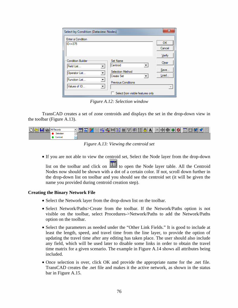
76

Figure A.12: Selection window

TransCAD creates a set of zone centroids and displays the set in the drop-down view in the toolbar (Figure A.13).

Figure A.13: Viewing the centroid set

• If you are not able to view the centroid set, Select the Node layer from the drop-down

list on the toolbar and click on to open the Node layer table. All the Centroid Nodes now should be shown with a dot of a certain color. If not, scroll down further in the drop-down list on toolbar and you should see the centroid set (it will be given the name you provided during centroid creation step).

Creating the Binary Network File

• Select the Network layer from the drop-down list on the toolbar.

• Select Network/Paths>Create from the toolbar. If the Network/Paths option is not visible on the toolbar, select Procedures->Network/Paths to add the Network/Paths option on the toolbar.

• Select the parameters as needed under the “Other Link Fields.” It is good to include at least the length, speed, and travel time from the line layer, to provide the option of updating the travel time after any editing has taken place. The user should also include any field, which will be used later to disable some links in order to obtain the travel time matrix for a given scenario. The example in Figure A.14 shows all attributes being included.

• Once selection is over, click OK and provide the appropriate name for the .net file. TransCAD creates the .net file and makes it the active network, as shown in the status bar in Figure A.15.

77

Figure A.14: Binary network creation window

Figure A.15: Status bar

Generating the Skims

• Select Network/Paths->Multiple Shortest Path from the toolbar. Make sure that Network file is selected in the drop-down list on the toolbar; otherwise, the Multiple Shortest Path option will not be available.

• Select Time under the Minimize option, and select Centroid for both the “From “and “To” fields. This step will ensure that all the calculation starts and ends at the centroid node (see Figure A.16).

78

Figure A.16: Multiple shortest path menu

• If the centroid set is not shown in the “From “and “To” option boxes, select All Features. This action will generate a shortest path for each Node pair. The disadvantage with this step is that once the matrix is generated, the user needs to remove the unnecessary node pair travel time.

• In order to generate the corresponding distance skim, click on Skims button as shown in Figure A.16 and select Length under Field option and chose All Links under Skim Type (Figure A.17). Click OK.

Figure A.17: Additional skim selection window

79

• Click OK one more time and TransCAD generates the shortest path travel time and corresponding distance matrix. To select the travel time matrix, select Time from the drop-down list on the toolbar (see Figure A.18).

Figure A.18: Toolbar

• To save the matrix, click on the toolbar. Matrices saved using this option are readable only by TransCAD.

• TransCAD also allows user to save the matrix in different formats. To export the matrix, select Matrix->Export and click OK (Figure A.19).

Figure A.19: Matrix export window

• TransCAD opens a window and asks the user for the file type. Select the desired file type under the option “Files of type”. We recommend the .txt or .csv format, as they are easy to view in Microsoft Excel. Note that this option does not save the skim in the matrix form. It will create a record per line for each non-empty cell in the original matrix.

• With this step, we finish the in-vehicle travel time and the corresponding travel distance matrix generation for each TAZ pair. The travel cost can now simply be calculated by assuming a Per Mile Gas cost and multiplying this with the corresponding travel distance. The out-of-vehicle travel time is generated based on TAZ area type. The typical value assumed by CAMPO is provided in Table A.1.

80

Table A.1: Out-of-vehicle travel time based on area type

Area Type Typical CAMPO Value

Central business district (CBD) 1.5 minutes

CBD Fringe 1.25 minutes

Urban and Suburban 1.00 minutes

Development of Skims for Bike and Walk

To generate the skim (distance matrix) for bike and walk modes, we assume that people tend to avoid freeway and highway segments when commuting in bike and walk modes. (Also, biking and walking are generally not allowed on freeways and highways.) So, to incorporate these effects in the network, the user needs to disable the freeway and highway links for these two modes.

• To disable the links, select Network/Paths->Settings on the toolbar. TransCAD opens a window as shown in Figure A.20.

Figure A.20: Network setting window

• Click on Update and select Disable Links and By Expression as shown in Figure A.21.

81

Figure A.21:Network update window

• Click OK, enter the condition in the Expression box, and then click OK twice. Here, we identify the freeway and highway network as functional classification 4 as shown in Figure A.22 (FUNCL=4).

Figure A.22: Condition window

• To ensure that the links have been disabled, click on Info as shown in Figure A.23 and TransCAD shows the information on disable links. You can click on the Info button at any time during the modeling process to check the network status.

82

Figure A.23: Network info window

• Run the Multiple Shortest Path on this network and minimize the distance. This will create the distance matrix for bike and walk mode with constrained network. Calculate the travel time matrix for the bike and walk by assuming average biking (11 mph) and walking (3 mph) speeds.

• TransCAD does not automatically enable the disabled links the next time you start a new session on the same network. In order to work with full network, select Network/Paths->Settings->Updates and select Enable Links and All Features as shown in Figure A.24.

Figure A.24: Re-enable all the links

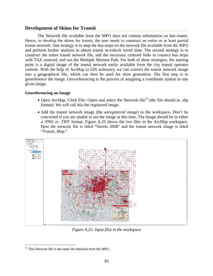
83

Development of Skims for Transit

The Network file available from the MPO does not contain information on bus routes. Hence, to develop the skims for transit, the user needs to construct an entire or at least partial transit network. One strategy is to map the bus stops on the network file available from the MPO and perform further analysis to obtain transit in-vehicle travel time. The second strategy is to construct the entire transit network file, add the necessary centroid links to connect bus stops with TAZ centroid, and run the Multiple Shortest Path. For both of these strategies, the starting point is a digital image of the transit network easily available from the city transit operator website. With the help of ArcMap (a GIS software), we can convert the transit network image into a geographical file, which can then be used for skim generation. The first step is to georeference the image. Geo-referencing is the process of assigning a coordinate system to any given image.

Georeferencing an Image

• Open ArcMap. Click File->Open and select the Network file15 (the file should in .shp format). We will call this the registered image.

• Add the transit network image (the unregistered image) to the workspace. Don’t be concerned if you are unable to see the image at this time. The image should be in either a .PNG or .TIFF format. Figure A.25 shows the two files in the ArcMap workspace. Here the network file is titled “Streets 2008” and the transit network image is titled “Transit_Map.”

Figure A.25: Input files in the workspace

15 This Network file is the same file obtained from the MPO.

84

• Select the Georeferencing tool: open the Customize menu, select Toolbars, and find Georeferencing. Fix the Georeferencing box on the toolbar by placing the box appropriately in the empty region of the ribbon. Figure A.26 shows the overview of the Georeferencing toolbar.

Figure A.26: Georeferencing toolbar

• To make the image visible within the workspace area, select the transit image in the Georeferencing toolbar as shown in Figure A.25 and select Fit to Display. This action might hide the registered image. Select the shift tool (Figure A.27) to drag the unregistered image to the side as shown in Figure A.28.

Figure A.27: Shift tool

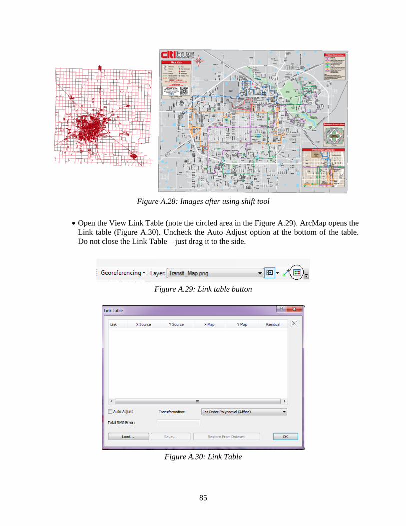
85

Figure A.28: Images after using shift tool

• Open the View Link Table (note the circled area in the Figure A.29). ArcMap opens the Link table (Figure A.30). Uncheck the Auto Adjust option at the bottom of the table. Do not close the Link Table—just drag it to the side.

Figure A.29: Link table button

Figure A.30: Link Table

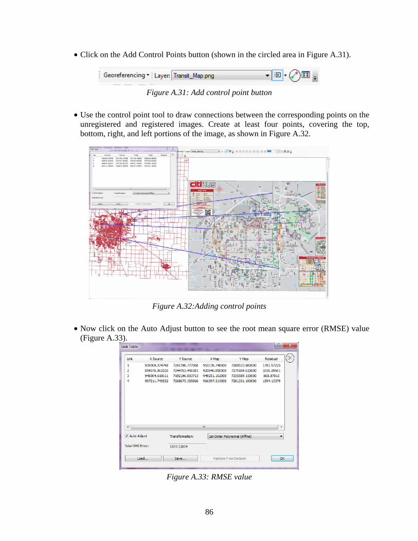
86

• Click on the Add Control Points button (shown in the circled area in Figure A.31).

Figure A.31: Add control point button

• Use the control point tool to draw connections between the corresponding points on the unregistered and registered images. Create at least four points, covering the top, bottom, right, and left portions of the image, as shown in Figure A.32.

Figure A.32:Adding control points

• Now click on the Auto Adjust button to see the root mean square error (RMSE) value (Figure A.33).

Figure A.33: RMSE value

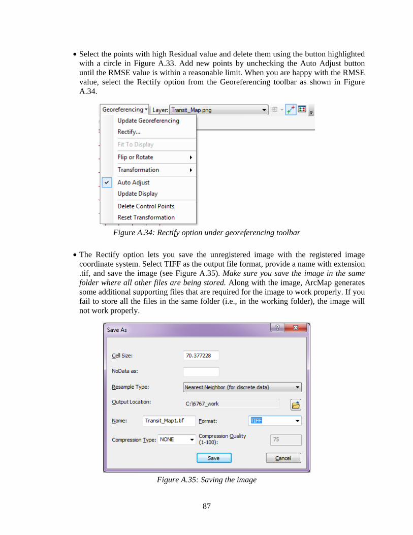
87

• Select the points with high Residual value and delete them using the button highlighted with a circle in Figure A.33. Add new points by unchecking the Auto Adjust button until the RMSE value is within a reasonable limit. When you are happy with the RMSE value, select the Rectify option from the Georeferencing toolbar as shown in Figure A.34.

Figure A.34: Rectify option under georeferencing toolbar

• The Rectify option lets you save the unregistered image with the registered image coordinate system. Select TIFF as the output file format, provide a name with extension .tif, and save the image (see Figure A.35). Make sure you save the image in the same folder where all other files are being stored. Along with the image, ArcMap generates some additional supporting files that are required for the image to work properly. If you fail to store all the files in the same folder (i.e., in the working folder), the image will not work properly.

Figure A.35: Saving the image

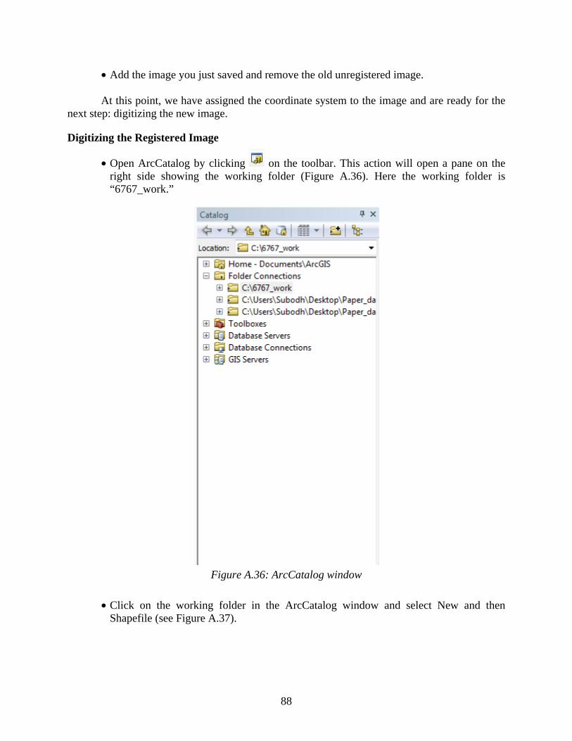
88

• Add the image you just saved and remove the old unregistered image. At this point, we have assigned the coordinate system to the image and are ready for the

next step: digitizing the new image.

Digitizing the Registered Image

• Open ArcCatalog by clicking on the toolbar. This action will open a pane on the right side showing the working folder (Figure A.36). Here the working folder is “6767_work.”

Figure A.36: ArcCatalog window

• Click on the working folder in the ArcCatalog window and select New and then Shapefile (see Figure A.37).

89

Figure A.37: Adding shapefile to the working folder

• This action opens a Shapefile box as shown in Figure A.38. Provide a name for the Shapefile and select the Feature Type “Point” to hold the stops and “Polyline” to hold the roads you will digitize; also select a new polygon Shapefile into which you will digitize fields. If the coordinate system is undefined, click on Edit to select from the various coordinate system options. If you know the coordinate system of the registered image exactly, assign the same to the Shapefile; otherwise, leave it undefined. (Note: undefined coordinate system files do present a problem: the user does not know the units of measurement. Once the file is created with appropriate data, trial and error is required to determine the unit of measurement. For example, once the bus stops are mapped into the shapefile, we assign a certain coordinate system to the shapefile and determine the distance between them using shapefile units and compare the obtained value with the true value. The procedure is repeated with different coordinate systems until a satisfactory result is obtained.) To assign a coordinate system at the time of the shapefile’s creation, click the Edit button to the define coordinate system (given various

90

options). If the shapefile is already created, right-click and select Properties. Both of these options lead to the same window as shown in Figure A.39.

Figure A.38: Shapefile property box

Figure A.39: Coordinate system window

91

• Again, in ArcCatalog, click on the working folder and select New->Personal GeoDatabase. Rename it appropriately. Do not change the .mbd extension.

• Click on the GeoDatabase and select New->Feature Dataset.

• Provide a name for the dataset followed by coordinate system. Click Next and Finish (see Figure A.40).

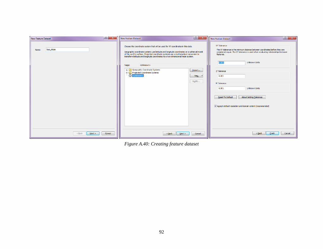
92

Figure A.40: Creating feature dataset

93

• Click on the Feature Dataset and select New->Feature Class. Provide a name for the Feature class and select the type. For bus stops, provide a name for the final bus stops (e.g., Final_Stops) and select Point Features from the Type drop-down menu. For bus links, provide a name for the final bus links (e.g., Final_bus_links) and select Line Features from the Type drop-down menu (see Figure A.41). Accept the default in the next window and click Finish.

Figure A.41: Feature class definition

• Both the shapefiles should appear in the Table of Contents window on the left side (see Figure A.42). If not, add them manually.

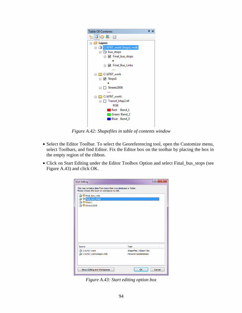
94

Figure A.42: Shapefiles in table of contents window

• Select the Editor Toolbar. To select the Georeferencing tool, open the Customize menu, select Toolbars, and find Editor. Fix the Editor box on the toolbar by placing the box in the empty region of the ribbon.

• Click on Start Editing under the Editor Toolbox Option and select Final_bus_stops (see Figure A.43) and click OK.

Figure A.43: Start editing option box

95

• This opens up a pane on the right side. Select Final_bus_stops and the program will highlight the Construction Tools at the bottom. Select the Point option as shown in Figure A.44.

Figure A.44: Create feature window

• Select the Point option from the Editor Toolbox (see the square blue box in Figure A.45) and start clicking on the image to digitize the points.

Figure A.45: Point option on Editor Toolbar

• Click on all the points you want to digitize and then click on Save Edits followed by Stop Editing (see Figure A.46).

96

Figure A.46: Save edits and stop editing options

• Now click on the Final_bus_stops Shapefile in the Table of Contents window and select Open Attribute Table. You should see the table similar to Figure A.47.

Figure A.47: Attribute table for bus stops

• At this point, we have the points and we do not know the coordinates of the points. Let’s add XY coordinate to the points. Click at the top of the table and select Add Fields as shown in Figure A.48.

97

Figure A.48: Add field option to table

• Provide a name (e.g., X_Cord) and under Type select Double (see Figure A.49). Repeat this step to add the Y_Cord field.

Figure A.49: Defining field name and type

• Now select the X_Cord field, then right-click and select Calculate Geometry. Next, select the X Coordinate of Point in the Property drop-down list and click OK. The X_Cord field gets populated with corresponding X coordinates (see Figure A.50). Do

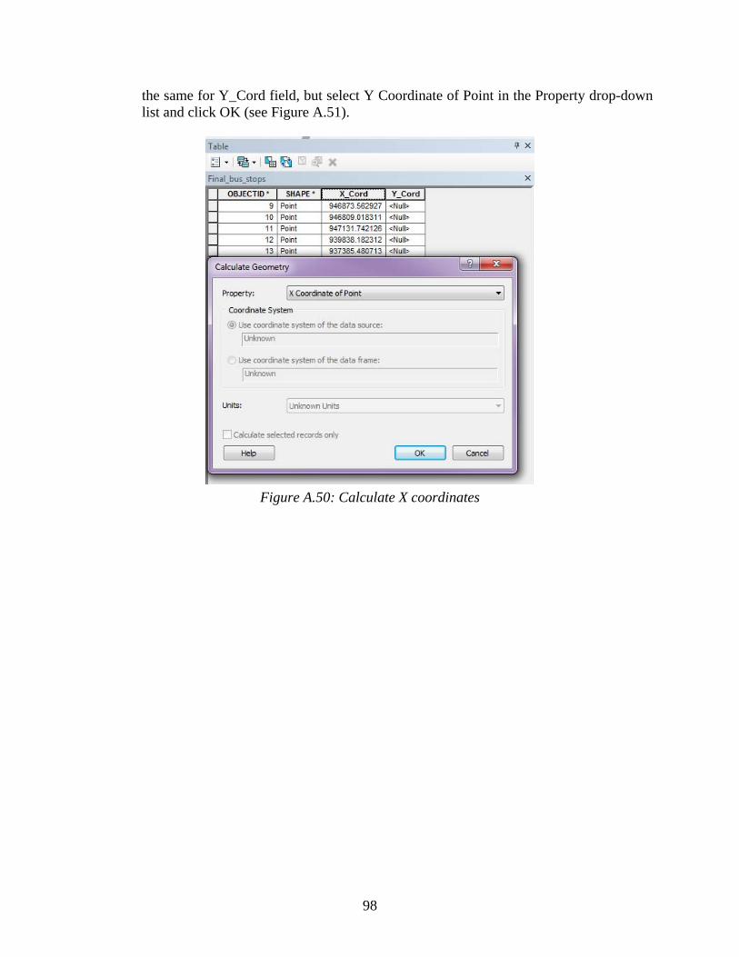
98

the same for Y_Cord field, but select Y Coordinate of Point in the Property drop-down list and click OK (see Figure A.51).

Figure A.50: Calculate X coordinates

99

Figure A.51: Calculate Y coordinates

This completes the digitization of bus stops from the image into a geographic file. Next, we turn our attention towards digitization of bus links. First we must set the snapping environment. ArcMap provides two ways to set the snapping environment (the new snapping tool or the classic snapping tool).

Setting the Snapping Environment

New snapping tool

• To use the new snapping tool, select Customize->Toolbars->Snapping. To select the tool, right-click on it. This display the snapping toolbar (see Figure A.52) as a floating toolbar, so drag it to reposition it.

Figure A.52: Snapping toolbar

100

• To set the snapping tolerance, click on the snapping toolbar and select Options (see Figure A.53). This action opens a window as shown in Figure A.54. Enter the tolerance value in pixel. (Unfortunately, we can set the tolerance only in pixels.) Generally, the images have about a 60-cm resolution, so for 4 meters, we can specify 7 pixels. To be on the safe side, use a value between 1 and 4.

Figure A.53: Snapping toolbar options

Figure A.54: New snapping tolerance setting window

101

Classic snapping tool

• To use the classic snapping tool, click on the Editor tool, then select Options from the bottom of the dropdown menu, then check the option Use Classic Snapping (see Figure A.55).

Figure A.55: Classic snapping option window

• To set the snapping tolerance, click on Editor, Snapping, and then Options (see Figure A.56). Set the snapping tolerance to around 4 map units.

102

Figure A.56: Classic snapping tolerance setting window

o Note: use either one of the snapping methods—do not use both. We recommend using the classic snapping option.

• To digitize the roads, click on Start Editing under the Editor Toolbox Option, and this time select Final_bus_links (see Figure A.57) and click OK.

• This action opens up a pane on the right side. Select the Final_bus_links to highlight the Construction Tools at the bottom. Select the Line option as shown in Figure A.57.

Figure A.57: Create feature window (line option)

• Select the Line option from the Editor Toolbox (see the square blue box in Figure A.58).

Figure A.58: Line option on Editor Toolbar

• To digitize the lines, move the cursor to the start of the road you wish to digitize, and click. Move along the center of the road and double-click to end the line. Use small

103

segments for higher accuracy. Each time you double-click on the image, a line will be added to the Final_bus_links shapefile (see Figure A.59).

Figure A.59: Final_bus_links shapefile

• To view the digitized lines, uncheck the image in the Table of Contents and you should see the lines you just digitized. Once the digitization of transit links is completed, add the attributes such as travel time, name, etc. using the Add Fields option discussed earlier.

• Save both the shapefiles Final_bus_stops and Final_bus_links when you are done editing. To save the files as separate shapefiles outside the database, right-click on the respective shapefiles (Final_bus_stops and Final_bus_links) and select Data->Export Data. You should see a window similar to Figure A.60. Click on the yellow output button (circled in black) and select Shapefile option in Save as type (see Figure A.61) and provide a name. Click Save and you are done.

Figure A.60: Data export window

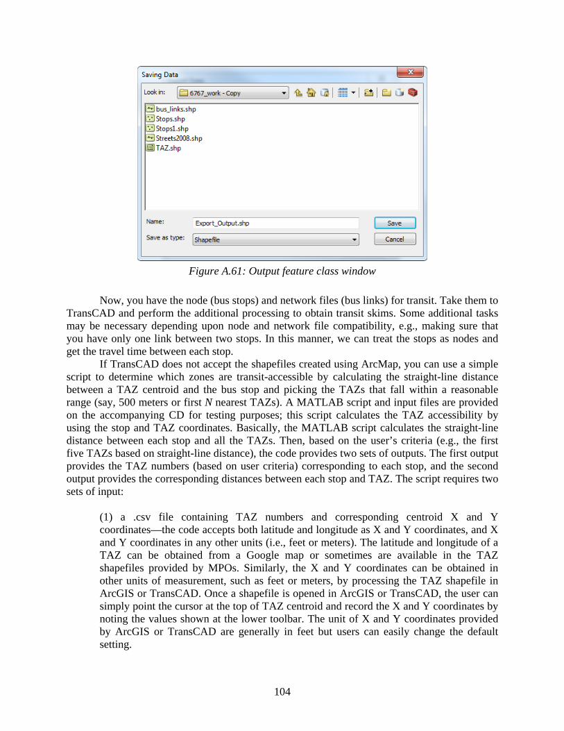
104

Figure A.61: Output feature class window

Now, you have the node (bus stops) and network files (bus links) for transit. Take them to TransCAD and perform the additional processing to obtain transit skims. Some additional tasks may be necessary depending upon node and network file compatibility, e.g., making sure that you have only one link between two stops. In this manner, we can treat the stops as nodes and get the travel time between each stop.

If TransCAD does not accept the shapefiles created using ArcMap, you can use a simple script to determine which zones are transit-accessible by calculating the straight-line distance between a TAZ centroid and the bus stop and picking the TAZs that fall within a reasonable range (say, 500 meters or first N nearest TAZs). A MATLAB script and input files are provided on the accompanying CD for testing purposes; this script calculates the TAZ accessibility by using the stop and TAZ coordinates. Basically, the MATLAB script calculates the straight-line distance between each stop and all the TAZs. Then, based on the user’s criteria (e.g., the first five TAZs based on straight-line distance), the code provides two sets of outputs. The first output provides the TAZ numbers (based on user criteria) corresponding to each stop, and the second output provides the corresponding distances between each stop and TAZ. The script requires two sets of input:

(1) a .csv file containing TAZ numbers and corresponding centroid X and Y coordinates—the code accepts both latitude and longitude as X and Y coordinates, and X and Y coordinates in any other units (i.e., feet or meters). The latitude and longitude of a TAZ can be obtained from a Google map or sometimes are available in the TAZ shapefiles provided by MPOs. Similarly, the X and Y coordinates can be obtained in other units of measurement, such as feet or meters, by processing the TAZ shapefile in ArcGIS or TransCAD. Once a shapefile is opened in ArcGIS or TransCAD, the user can simply point the cursor at the top of TAZ centroid and record the X and Y coordinates by noting the values shown at the lower toolbar. The unit of X and Y coordinates provided by ArcGIS or TransCAD are generally in feet but users can easily change the default setting.

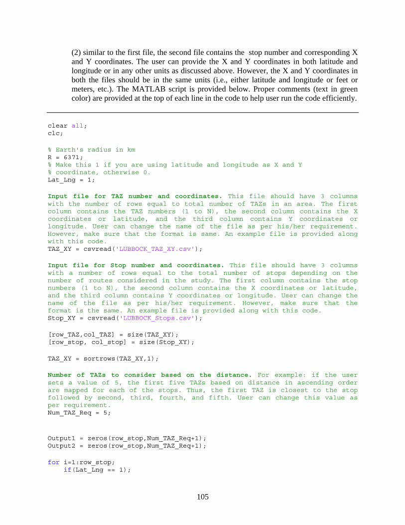
105

(2) similar to the first file, the second file contains the stop number and corresponding X and Y coordinates. The user can provide the X and Y coordinates in both latitude and longitude or in any other units as discussed above. However, the X and Y coordinates in both the files should be in the same units (i.e., either latitude and longitude or feet or meters, etc.). The MATLAB script is provided below. Proper comments (text in green color) are provided at the top of each line in the code to help user run the code efficiently.

clear all; clc; % Earth's radius in km R = 6371; % Make this 1 if you are using latitude and longitude as X and Y % coordinate, otherwise 0. Lat_Lng = 1; Input file for TAZ number and coordinates. This file should have 3 columns with the number of rows equal to total number of TAZs in an area. The first column contains the TAZ numbers (1 to N), the second column contains the X coordinates or latitude, and the third column contains Y coordinates or longitude. User can change the name of the file as per his/her requirement. However, make sure that the format is same. An example file is provided along with this code. TAZ_XY = csvread('LUBBOCK_TAZ_XY.csv'); Input file for Stop number and coordinates. This file should have 3 columns with a number of rows equal to the total number of stops depending on the number of routes considered in the study. The first column contains the stop numbers (1 to N), the second column contains the X coordinates or latitude, and the third column contains Y coordinates or longitude. User can change the name of the file as per his/her requirement. However, make sure that the format is the same. An example file is provided along with this code. Stop_XY = csvread('LUBBOCK_Stops.csv'); [row_TAZ,col_TAZ] = size(TAZ_XY); [row_stop, col_stop] = size(Stop_XY); TAZ_XY = sortrows(TAZ_XY,1); Number of TAZs to consider based on the distance. For example: if the user sets a value of 5, the first five TAZs based on distance in ascending order are mapped for each of the stops. Thus, the first TAZ is closest to the stop followed by second, third, fourth, and fifth. User can change this value as per requirement. Num_TAZ_Req = 5; Output1 = zeros(row_stop,Num_TAZ_Req+1); Output2 = zeros(row_stop,Num_TAZ_Req+1); for i=1:row_stop; if(Lat_Lng == 1);

106

Temp_Dist = zeros(row_TAZ,2); for j=1:row_TAZ; delta_lat = Stop_XY(i,2) - TAZ_XY(j,2) ; delta_lon = Stop_XY(i,3) - TAZ_XY(j,3) ;

a = sin(delta_lat/2)^2 + cos(TAZ_XY(j,2)) * cos(Stop_XY(i,2)) * sin(delta_lon/2)^2;

c = 2 * atan2(sqrt(a), sqrt(1-a)); Temp_Dist(j,1) = TAZ_XY(j,1); Temp_Dist(j,2) = R * c; end; Temp_Dist = sortrows(Temp_Dist,2); Output1(i,1) = Stop_XY(i,1); Output2(i,1) = Stop_XY(i,1); Output1(i,2:Num_TAZ_Req+1) = (Temp_Dist(1:Num_TAZ_Req,1))'; Output2(i,2:Num_TAZ_Req+1) = (Temp_Dist(1:Num_TAZ_Req,2))'; clear Temp_Dist; else Temp_Dist = zeros(row_TAZ,2); for j=1:row_TAZ; X_Diff = Stop_XY(i,2) - TAZ_XY(j,2) ; Y_Diff = Stop_XY(i,3) - TAZ_XY(j,3) ; a = sqrt(X_Diff^2 + Y_Diff^2); Temp_Dist(j,1) = TAZ_XY(j,1); Temp_Dist(j,2) = a; end; Temp_Dist = sortrows(Temp_Dist,2); Output1(i,1) = Stop_XY(i,1); Output2(i,1) = Stop_XY(i,1); Output1(i,2:Num_TAZ_Req+1) = (Temp_Dist(1:Num_TAZ_Req,1))'; Output2(i,2:Num_TAZ_Req+1) = (Temp_Dist(1:Num_TAZ_Req,2))'; clear Temp_Dist; end; end; First output file providing the list of TAZs (TAZ numbers) for each of the stops. The first column contains the stop number in each row and the remaining columns contain the TAZ numbers. That is, if the first row of the file has a value of 1 115 118 117, then the 1 indicates the stop number and 115, 118, and 117 indicate the TAZ numbers in the ascending order of distance. dlmwrite('Stop_TAZ_Map.csv',Output1,'delimiter',',',precision,15); Second output file providing the distance between the stop and the TAZs. Please note that the distances reported in this file are in the same order as the TAZs reported in first file. That is, if the first row of the file has a value 1 70.45 200.32 550.43, then the 1 indicates the stop number and 70.45, 200.32, and 550.43 indicate the distance between stop 1 and TAZs 115, 118, and 117 respectively. All the other rows can be interpreted in the same way as discussed. Remember that if the X & Y coordinates are latitude and longitude, then the unit of distance is kilometer; otherwise, it is the same as the unit of the X & Y coordinates. dlmwrite('Stop_TAZ_Dist.csv',Output2,'delimiter',',',precision,15); disp 'Done'; ---------------------------------------------------------------------------------------------------------------------

107

Appendix B. Forecasting Tool User Manual

Introduction

The Excel-based forecasting tool allows users to provide a mode choice model along with various skims (in-vehicle travel time, out-of-vehicle travel time, travel distance, and travel cost) in order to calculate the mode share at both the traffic analysis zone (TAZ) level and individual level. It also has the capability of obtaining the mode share given any change in the model explanatory variables—such as in-vehicle travel time, out-of-vehicle travel time, etc.—via the tool’s scenario module.

Input

Figure B.1 shows the main “INPUT” sheet of the tool (the red tab); the single input sheet tabs appear along the bottom. To make the tool user-friendly, all the sheets in the tool are named according to their functionality. The user needs to appropriately fill in all 11 sheets to run the tool. In contrast to the main “INPUT” sheet, the single input sheets have green tabs (see Figure B.1).

108

Figure B.1: Forecasting Tool Input Sheet

109

Input Requirements

Table B.1 provides the name and the type of data required for entry into the input sheets.

Table B.1: Sheet Name and Data Requirement

Sheet Name Description/Functionality

INPUT User needs to provide the mode choice model and various other inputs as mentioned in the sheet (refer to Table B.3 for a detailed discussion).

INDIVIDUAL_RECORDS If user has the individual-level trip distribution records, provide them in this sheet in the format specified at the top of the sheet.

TAZ_HH_INCOME_DATA This sheet accepts the TAZ level household split in percentage based on household size and household annual income (refer to the sheet in the tool for a sample input).

IVTT_DA This sheet accepts the in-vehicle travel time matrix for Drive Alone mode; i.e., TAZ-TAZ in-vehicle travel time.

AREA_TYPE

This sheet accepts the area classification indicator variable for each TAZ (refer to Table B.2 for area classification code). This is used to calculate out-of-vehicle travel time for the Drive Alone and Shared Ride modes.

DISTANCE_DA This sheet accepts the travel distance matrix corresponding to the shortest path travel time matrix for Drive Alone mode; i.e., TAZ-TAZ travel distance.

IVTT_TRANSIT This sheet accepts the in-vehicle travel time matrix for Transit mode; i.e., TAZ-TAZ in-vehicle travel time.

OVTT_TRANSIT This sheet accepts the travel time to the nearest bus stop for a TAZ in a matrix format; i.e., each cell represents the walking time to the nearest bus stop for the corresponding TAZ.

DISTANCE_TRANSIT This sheet accepts the travel distance matrix for Transit mode; i.e., TAZ-TAZ travel distance.

DISTANCE_BIKE This sheet accepts the travel distance matrix for Bike mode; i.e., TAZ-TAZ travel distance.

DISTANCE_WALK This sheet accepts the travel distance matrix for Walk mode; i.e., TAZ-TAZ travel distance.

110

Please note that all the skims sheets (IVTT_DA, DISTANCE_DA, IVTT_TRANSIT, OVTT_TRANSIT, DISTANCE_TRANSIT, DISTANCE_BIKE, and DISTANCE_WALK) should be symmetrical—the number of rows should equal the number of columns. If the sizes for all the skims sheets are not same, the program will return an error message. In cases where no transit service is available between any TAZ pair, simply provide a value of zero in the corresponding cell. However, for Drive Alone, the user must provide a non-negative in-vehicle travel time and travel distance value. Table B.2 provides the area classification codes. Please note that the area classification provided here is an example of the many classifications used by various metropolitan planning organizations (MPOs). Users can choose any classification based on their requirements.

Table B.2: Out-of-Vehicle Travel Time Based on Area Type

Area Type Classification Code Out-of-Vehicle Travel

Time*

Central Business District (CBD) (1) 1 1.5 mins

CBD Fringe 2 1.25 mins

Urban and Suburban 3 & 4 1.00 mins

*Travel times used by the Capital Area Metropolitan Planning Organization (CAMPO)

“INPUT” Sheet Details

Table B.3 provides the detail of the main sheet named “INPUT”, where users can change the value of various inputs.

Table B.3: INPUT Sheet Detail

Input Name Description

Number of TAZ Provide the total number of internal TAZs. This number must not exceed the size of skim sheet matrix.

Per Mile Gas Cost (in dollars)

Provide per-mile gas cost for Drive Alone mode.

Average Bike Speed (mph)

Provide the value of average bike speed. Generally, a value of 11 mph is used by various MPOs.

Average Walk Speed (mph)

Provide the value of average walk speed. Generally, a value of 3 mph is used by various MPOs.

Transit Fare (dollars) Provide the transit fare applicable to the area under analysis.

Number of Area Classification

Provide the total number of area classification used in the analysis. This number should exactly equal the number of rows in the Area Type/Wait Time table (see Figure B.1 or refer to this sheet in the tool).

111


Number of Passengers in Car for Shared Ride

Provide the number of passengers for Shared Ride mode.

Maximum Walk Time (min)

Provide maximum walk time acceptable to the user. It is used to determine the walk availability between TAZ pairs

Maximum Bike Time (min)

Provide maximum bike time acceptable to the user. This figure is used to determine the bike availability between TAZ pairs.

Put 1 if you want to limit the availability of Walk mode based on maximum walk time

Make this 1 if you want to limit the availability of Walk mode based on maximum walk time during mode share calculation; otherwise, enter 0.

Put 1 if you want to limit the availability of Bike mode based on maximum bike time

Make this 1 if you want to limit the availability of Bike mode based on maximum bike time during mode share calculation; otherwise, enter 0.

Individual level estimates

Make this 1 if you want to run the individual-level estimates. This is applicable only when the user provides individual-level trip distribution data in the sheet named “INDIVIDUAL_RECORDS”; otherwise, enter 0.

TAZ level estimates

Make this 1 if you want to run the TAZ-level estimates. This is applicable under any circumstance because TAZ-level household information is available readily from the Texas Package. However, only one of the two options should be enabled at a time.

Number of Alternatives

Provide the total number of alternatives in the model. It should be equal to the number of alternatives provided in the model.

Number of Explanatory Variables Including Constants

Provide the number as mentioned.

Create TAZ Configuration

Make this 1 if you want to create a TAZ-TAZ skim configuration.

Household Category Provide the number of household category used in the model; i.e., household classification based on household size

Income Category Provide the number of income category used in the model; i.e., household classification based on income range.

Scenario (Alternative Related Variables)

Make this 1 if you want to obtain the mode shares under the scenario change option.

Reduce Transit IVTT (in Percentage)

Provide a number to reduce transit in-vehicle travel time by a certain percentage. Enter only a numeral—do not add a positive/negative sign at the beginning or the % sign at the end.

112


Increase Drive Alone IVTT (in Percentage)

Provide a number to increase Drive Alone in-vehicle travel time by a certain percentage. Enter only a numeral—do not add a positive/negative sign at the beginning or the % sign at the end.

Increase Drive Alone OVTT (in Percentage)

Provide a number to increase Drive Alone out-of-vehicle travel time by a certain percentage. Enter only a numeral—do not add a positive/negative sign at the beginning or the % sign at the end.

The user must also provide values for the Area Type/Wait Time table, located between the main input listing and the parameters table, as shown in Figure B.1. Do not change the position of any input item, as doing so may cause problems during calculation.

Mode Share Estimation

With everything set, proceed to the four buttons that appear underneath the parameters table on the main “INPUT” page. The buttons need to be clicked sequentially from 1 to 4. First, click the button “REFRESH ALL (1)”. This button’s function is to remove any sheets left from previous runs. After this, click the button “CLICK TO CHECK DATA (2)”. It checks for lack of data consistency such as empty cells, inappropriate value, etc., and warns the user if any are found, prompting the user to address any inappropriate values. For ease in handling, a message will pop up describing the problem along with the sheet name, and the corresponding cell in the sheet will be colored green for easy identification. For example: Suppose that the first cell in the sheet “IVTT_DA” is empty. When the user clicks the button “CLICK TO CHECK DATA (2)”, a message will pop up (see Figure B.2) and the program will be terminated. The user now can go to the corresponding sheet, find the empty cell (highlighted with green as shown in Figure B.3), change the value accordingly, and re-click the same button.

Figure B.2: Empty Cell Message

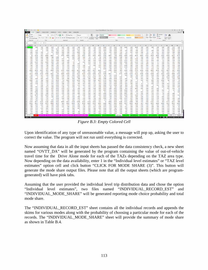
113

Figure B.3: Empty Colored Cell

Upon identification of any type of unreasonable value, a message will pop up, asking the user to correct the value. The program will not run until everything is corrected. Now assuming that data in all the input sheets has passed the data consistency check, a new sheet named “OVTT_DA” will be generated by the program containing the value of out-of-vehicle travel time for the Drive Alone mode for each of the TAZs depending on the TAZ area type. Now depending on the data availability, enter 1 in the “Individual level estimates” or “TAZ level estimates” option cell and click button “CLICK FOR MODE SHARE (3)”. This button will generate the mode share output files. Please note that all the output sheets (which are program-generated) will have pink tabs. Assuming that the user provided the individual level trip distribution data and chose the option “Individual level estimates”, two files named “INDIVIDUAL_RECORD_EST” and “INDIVIDUAL_MODE_SHARE” will be generated reporting mode choice probability and total mode share. The “INDIVIDUAL_RECORD_EST” sheet contains all the individual records and appends the skims for various modes along with the probability of choosing a particular mode for each of the records. The “INDIVIDUAL_MODE_SHARE” sheet will provide the summary of mode share as shown in Table B.4.

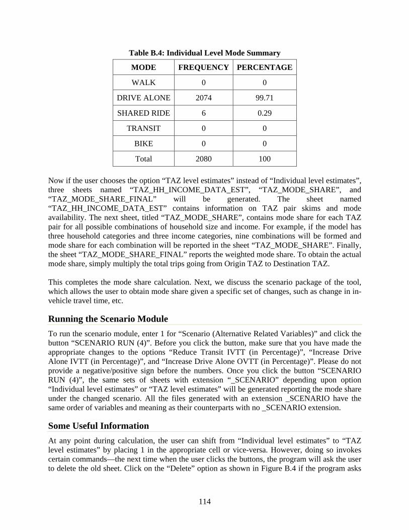
114

Table B.4: Individual Level Mode Summary

MODE FREQUENCY PERCENTAGE

WALK 0 0

DRIVE ALONE 2074 99.71

SHARED RIDE 6 0.29

TRANSIT 0 0

BIKE 0 0

Total 2080 100

Now if the user chooses the option “TAZ level estimates” instead of “Individual level estimates”, three sheets named “TAZ_HH_INCOME_DATA_EST”, “TAZ_MODE_SHARE”, and “TAZ_MODE_SHARE_FINAL” will be generated. The sheet named “TAZ_HH_INCOME_DATA_EST” contains information on TAZ pair skims and mode availability. The next sheet, titled “TAZ_MODE_SHARE”, contains mode share for each TAZ pair for all possible combinations of household size and income. For example, if the model has three household categories and three income categories, nine combinations will be formed and mode share for each combination will be reported in the sheet “TAZ_MODE_SHARE”. Finally, the sheet “TAZ_MODE_SHARE_FINAL” reports the weighted mode share. To obtain the actual mode share, simply multiply the total trips going from Origin TAZ to Destination TAZ. This completes the mode share calculation. Next, we discuss the scenario package of the tool, which allows the user to obtain mode share given a specific set of changes, such as change in in-vehicle travel time, etc.

Running the Scenario Module

To run the scenario module, enter 1 for “Scenario (Alternative Related Variables)” and click the button “SCENARIO RUN (4)”. Before you click the button, make sure that you have made the appropriate changes to the options “Reduce Transit IVTT (in Percentage)”, “Increase Drive Alone IVTT (in Percentage)”, and “Increase Drive Alone OVTT (in Percentage)”. Please do not provide a negative/positive sign before the numbers. Once you click the button “SCENARIO RUN (4)”, the same sets of sheets with extension “_SCENARIO” depending upon option “Individual level estimates” or “TAZ level estimates” will be generated reporting the mode share under the changed scenario. All the files generated with an extension _SCENARIO have the same order of variables and meaning as their counterparts with no _SCENARIO extension.

Some Useful Information

At any point during calculation, the user can shift from “Individual level estimates” to “TAZ level estimates” by placing 1 in the appropriate cell or vice-versa. However, doing so invokes certain commands—the next time when the user clicks the buttons, the program will ask the user to delete the old sheet. Click on the “Delete” option as shown in Figure B.4 if the program asks

115

you to do so and then re-click the same button. Accepting the “Delete” option removes any unnecessary files.

Figure B.4: Delete the Old Sheets

Also, you will need to enable the Macro option available in Excel in order to run this tool. By default, when you open the tool, it will ask you to enable the Macro. Please accept the option. If the macro-enable option does not pop up in the beginning, follow this procedure:

Click the Microsoft Office Button , and then click Excel Options.

Click Trust Center, click Trust Center Settings, and then click Macro Settings.

Enable all macros (not recommended, potentially dangerous code can run). Click this option to allow all macros to run. This setting makes your computer vulnerable to potentially malicious code and is not recommended.

TIP: You can open the macro security settings dialog box from the Developer tab in the Ribbon, which is part of the Microsoft Office Fluent user interface. If the Developer tab is not available,

click the Microsoft Office Button , and then click Excel Options. Click Popular, and then select the Show Developer tab in the Ribbon check box.

117

Appendix C. The Multinomial Logit (MNL) Model

Consider a decision-maker that has to choose one alternative among several available alternatives, as depicted in Figure C.1. The multinomial logit (MNL) model is a discrete choice model that allows researchers to identify the factors influencing mode choice and forecast a future scenario to evaluate transportation policies.

Figure C.1: Mode choice framework of MNL models

The MNL model is based on the utility maximization theory. The utility function has two components: a deterministic (or observable) component that represents the portion of the utility observed by the analyst, and an unknown (or unobserved) component. Formally, the utility is as shown in Equation C.1: Equation C.1: MNL utility function

qiqiqi VU ε+=

qiU true utility of the alternative i to the decision-maker q

qiV deterministic or observable portion of the utility estimated by the analyst, for alternative i and decision-maker q

qiε error or the portion of the utility unknown to the analyst, for alternative i and decision-maker q

The deterministic or observable portion of the utility of an alternative qiV is a

mathematical function of the attributes of the alternative and the characteristics of the decision-maker. The systematic portion of utility can have any mathematical form but the function is most generally formulated as additive to simplify the estimation process, as shown in Equation C.2:

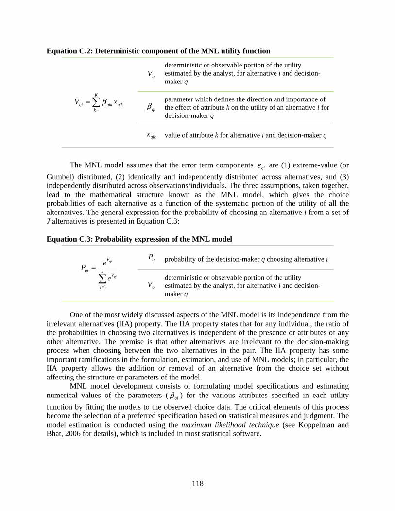
118

Equation C.2: Deterministic component of the MNL utility function

=

=K

kqikqikqi xV β


qiβ parameter which defines the direction and importance of the effect of attribute k on the utility of an alternative i for decision-maker q

qikx value of attribute k for alternative i and decision-maker q

The MNL model assumes that the error term components qiε are (1) extreme-value (or

Gumbel) distributed, (2) identically and independently distributed across alternatives, and (3) independently distributed across observations/individuals. The three assumptions, taken together, lead to the mathematical structure known as the MNL model, which gives the choice probabilities of each alternative as a function of the systematic portion of the utility of all the alternatives. The general expression for the probability of choosing an alternative i from a set of J alternatives is presented in Equation C.3: Equation C.3: Probability expression of the MNL model

=

=J

j

V

V

qiqj

qi

e

eP

1

qiP probability of the decision-maker q choosing alternative i


One of the most widely discussed aspects of the MNL model is its independence from the

irrelevant alternatives (IIA) property. The IIA property states that for any individual, the ratio of the probabilities in choosing two alternatives is independent of the presence or attributes of any other alternative. The premise is that other alternatives are irrelevant to the decision-making process when choosing between the two alternatives in the pair. The IIA property has some important ramifications in the formulation, estimation, and use of MNL models; in particular, the IIA property allows the addition or removal of an alternative from the choice set without affecting the structure or parameters of the model.

MNL model development consists of formulating model specifications and estimating numerical values of the parameters ( qiβ ) for the various attributes specified in each utility

function by fitting the models to the observed choice data. The critical elements of this process become the selection of a preferred specification based on statistical measures and judgment. The model estimation is conducted using the maximum likelihood technique (see Koppelman and Bhat, 2006 for details), which is included in most statistical software.

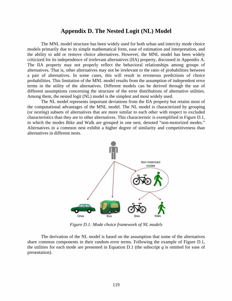
119

Appendix D. The Nested Logit (NL) Model

The MNL model structure has been widely used for both urban and intercity mode choice models primarily due to its simple mathematical form, ease of estimation and interpretation, and the ability to add or remove choice alternatives. However, the MNL model has been widely criticized for its independence of irrelevant alternatives (IIA) property, discussed in Appendix A. The IIA property may not properly reflect the behavioral relationships among groups of alternatives. That is, other alternatives may not be irrelevant to the ratio of probabilities between a pair of alternatives. In some cases, this will result in erroneous predictions of choice probabilities. This limitation of the MNL model results from the assumption of independent error terms in the utility of the alternatives. Different models can be derived through the use of different assumptions concerning the structure of the error distributions of alternative utilities. Among them, the nested logit (NL) model is the simplest and most widely used.

The NL model represents important deviations from the IIA property but retains most of the computational advantages of the MNL model. The NL model is characterized by grouping (or nesting) subsets of alternatives that are more similar to each other with respect to excluded characteristics than they are to other alternatives. This characteristic is exemplified in Figure D.1, in which the modes Bike and Walk are grouped in one nest, denoted “non-motorized modes.” Alternatives in a common nest exhibit a higher degree of similarity and competitiveness than alternatives in different nests.

Figure D.1: Mode choice framework of NL models

The derivation of the NL model is based on the assumption that some of the alternatives share common components in their random error terms. Following the example of Figure D.1, the utilities for each mode are presented in Equation D.1 (the subscript q is omitted for ease of presentation).

120

Equation D.1: Utility expressions for NL model of Figure D.1

drivedrivedrive VU ε+=

busbusbus VU ε+=

motorizednonbikebikebike VU −++= εε

motorizednonwalkwalkwalk VU −++= εε

iU true utility of the alternative i (i = drive, i = bus, i = bike or i = walk)

iV deterministic or observable portion of the utility estimated by the analyst, for alternative i (i = drive, i = bus, i = bike or i = walk)

iε error or the portion of the utility unknown to the analyst, for alternative i (i = drive, i = bus, i = bike or i = walk)

motorizednon−ε error or the portion of the utility unknown to the analyst, for non-motorized modes (bike or walk)

It is convenient to interpret this structure as if there are two levels of choice even though the derivation of the model makes no assumptions about the structure of the choice process. Figure D.1 depicts an upper level (marginal) choice among Drive Alone, Bus, and Non-Motorized modes and a lower level (conditional) choice between Bike and Walk, given that a non-motorized mode is chosen.

121

Appendix E. Travel Demand Models of MPOs Outside of Texas

Champaign County Regional Planning Commission (CCRPC, Illinois)

• CCRPC is located in Illinois and serves the Champaign-Urbana-Savoy-Bondville urbanized area, which comprises a population of 144,361 (comparable to small MPOs in Texas).

• As part of the 2025 long-range transportation plan, the study area was divided into 206 TAZs. The main source of data was the Champaign-Urbana Urbanized Area Transportation Study’s 2002–2003 Household Travel Survey. Trip productions and attraction rates are estimated for five trip purposes (HB work, HB school, HB shopping, HB other, and NHB). A cross-classification method was used to model trip productions, based on household size data. Trip attraction rates were borrowed and modified from the NCHRP Report 365.

Lincoln MPO (Nebraska)

• Lincoln MPO is located in Nebraska and serves the Lancaster County area, with a population of 285,407 (comparable to medium/small-sized MPOs in Texas).

• The study area was divided into 502 TAZs. The main source of data was the North Front Range Household Survey, which was the dataset most similar to the Lincoln MPO’s. Trip productions and attractions rates are estimated for seven trip purposes (HB work, HB shopping, HB recreational, HB university, HB other, work-based, and other). A cross-classification method was used to model trip productions, based on household size and income data. Trip attraction rates were taken from the previous Lincoln MPO model and adjusted to balance trip production rates.

Genesee County Metropolitan Planning Commission (GCMPC, Michigan)

• GCMPC is located in Michigan and serves the Genesee County area, with a population of 425,790 (comparable to medium/small-sized MPOs in Texas).

• The study area was divided into 639 TAZs. The main source of data was the Michigan Travel Counts Survey. Trip productions and attraction rates were estimated for eight trip purposes (HB work low-income, HB work high-income, HB shopping, HB other, HB school, HB university, NHB other, and NHB work). A cross-classification model was used to model trip productions, based on number of workers, vehicles per household, household size, and household income data. Trip attraction rates were calculated using a linear regression model calibrated by the Michigan Travel Counts database, specifically employment variables, total employment, and total number of households’ data.

Association of Monterey Bay Area Governments (AMBAG, California)

• The AMBAG MPO is located in California and serves the Santa Cruz, Monterey, and San Benito counties, with a combined population of 733,667 (comparable to medium/large-sized MPOs in Texas).

122

• The study area was divided into 1,884 TAZs. The main sources of data were the 2000–2001 California Statewide Household Travel Survey and the 2002 Monterey/San Benito Household Travel Survey. Trip production and attraction rates are estimated for seven trip purposes (HB work, HB maintenance, HB discretionary, work-based, HB school, other, and visitor from private residence or hotel rooms). A cross-classification method was used to model trip productions, based on income quartile, age of head of household, and auto ownership data. Trip attraction rates were borrowed and modified from the NCHRP Report 365 when not available from survey data.

Metro MPO (Oregon)

• Metro MPO is located in Oregon and serves Clackamas, Multnomah, and Washington counties, comprising a population of 285,407 (compared to large MPOs in Texas).

• The study area was divided into 2013 TAZs. The main source of data was the 1985 Household Travel Survey. Trip production and attraction rates are estimated for eight trip purposes (HB work, HB shopping, HB recreation, HB other, NHB work, NHB non-work, HB college, and HB school). A cross-classification model was used to model trip productions that were based on household size, number of workers, age of household head, number of children, and household size by worker status. Trip attraction rates are no longer computed, except for HB work and HB college attractions, which are calculated and then scaled to production rates.

developing a mode choice model for small and medium … · developing a mode choice model for small...

Documents