deterrence and legitimacy in anti-corruption policymaking · aper series african development bank...
TRANSCRIPT

African
Develop
ment Ba
nk Grou
p
Working
Pape
r Serie
s
n°277
July 2
017
Deterrence and Legitimacy in Anti-Corruption Policymaking Amadou Boly, Robert Gillanders and Topi Miettinen

Working Paper No 277
Abstract
In our framed laboratory experiment, two Public
Officials, A and B, make consecutive decisions
regarding embezzlement from separate funds.
Official B observes Official A’s decisions before
making his/her own. We find a contagion effect in
embezzlement in that facing a corrupt Official A
increases the likelihood and extent of embezzlement
by Official B. Likewise, deterrence matters in that
higher detection probabilities significantly decrease
the likelihood and extent of embezzlement.
Crucially, when the same deterrence policy applies
to both officials, detection is more effective in
curbing embezzlement if chosen by an honest public
official A rather than a corrupt Public Official A.
This legitimacy effect may help explain why anti-
corruption policies can fail in countries where the
government itself is believed (or known) to be
corrupt.
This paper is the product of the Vice-Presidency for Economic Governance and Knowledge Management. It is part
of a larger effort by the African Development Bank to promote knowledge and learning, share ideas, provide open
access to its research, and make a contribution to development policy. The papers featured in the Working Paper
Series (WPS) are those considered to have a bearing on the mission of AfDB, its strategic objectives of Inclusive
and Green Growth, and its High-5 priority areas—to Power Africa, Feed Africa, Industrialize Africa, Integrate
Africa and Improve Living Conditions of Africans. The authors may be contacted at [email protected].
Rights and Permissions
All rights reserved.
The text and data in this publication may be reproduced as long as the source is cited. Reproduction for commercial purposes
is forbidden. The WPS disseminates the findings of work in progress, preliminary research results, and development
experience and lessons, to encourage the exchange of ideas and innovative thinking among researchers, development
practitioners, policy makers, and donors. The findings, interpretations, and conclusions expressed in the Bank’s WPS are
entirely those of the author(s) and do not necessarily represent the view of the African Development Bank Group, its Board
of Directors, or the countries they represent.
Working Papers are available online at https://www.afdb.org/en/documents/publications/working-paper-series/
Produced by Macroeconomics Policy, Forecasting, and Research Department
Coordinator
Adeleke O. Salami
Correct citation: Boly A., R. Gillanders and T.Miettinen (2017), Deterrence and Legitimacy in Anti-Corruption Policymaking,
Working Paper Series N° 277, African Development Bank, Abidjan, Côte d’Ivoire.
1
Deterrence and Legitimacy in Anti-Corruption Policymaking1
Amadou Boly, Robert Gillanders and Topi Miettinen
JEL codes: C91, D73, K42.
Keywords: Contagion effect, Corruption, Deterrence, Embezzlement, Laboratory Experiment,
Legitimacy.
1 Amadou Boly, African Development Bank (AfDB), Development Research Department, Abidjan, Côte d’Ivoire.
Corresponding author email: [email protected]
Robert Gillanders, Dublin City University Business School and Hanken School of Economics. email:
Topi Miettinen, Hanken School of Economics, Department of Economics, P.O. Box 479, FI-00101 Helsinki,
Finland. email: [email protected].
This research is reproduced here with acknowledgement to UNU-WIDER in Helsinki which commissioned the
original study. The views expressed here are those of the authors and do not necessarily represent or reflect those
of the Institute, the United Nations University, the programme/project sponsors, nor the African Development
Bank.
We thank the Busara Center for Behavioral Economics for conducting the experiments. We would also like to
thank participants at the African Development Bank internal seminar series, the 2016 Canadian Economic
Association Annual Conference, the 2016 PEGNet Conference, and the UNU-MERIT/MGSoG seminar series for
comments and suggestions.
2
1 Introduction
Corruption has been found to have undesirable effects on key economic metrics such as
macroeconomic growth (Mauro 1995), firm growth (Fisman and Svensson 2007), and income
equality and poverty (Gupta et al. 2002). On account of these large costs of corruption and the
fact that corruption is particularly prevalent in developing and transition economies, anti-
corruption laws and policies often constitute important elements in both internally and
externally initiated reforms. A commonly advocated anti-corruption approach is deterrence,
which is justified by appeals to models of rational criminal behaviour. These models assume
that an illegal act, such as corruption, is preferred and chosen if its net expected benefit is higher
than that of legal alternatives (e.g. Becker 1968; Eide et al. 2006). As a result, government
authorities can increase compliance with the law by increasing the risks (probability of
detection) and/or costs (severity of sanctions) associated with illegal acts.
The available experimental evidence suggests that the existence of a probability of
detection and punishment can indeed curb corruption (for example: Abbink et al. 2002; Olken
2007; Hanna et al. 2011). In a typical corruption experiment, a control treatment with zero
detection probability is compared to an experimental treatment with one positive level of
detection probability exogenously imposed by the researcher (see e.g. Abbink et al. 2002; Serra
2012). The present paper builds on this literature by considering environments in which the
level of the detection is endogenously chosen, allowing us to analyse the role of legitimacy in
anti-corruption policy making.2 Specifically, in our framed corruption experiment conducted
in Kenya, there are two Public Officials, called A and B. They both receive a salary and are
entrusted with separate funds to be spent on social projects. Each public official has the
opportunity to embezzle from the fund under his/her control before sending the remaining
amount to a recipient. The recipient is different for each public official and is chosen randomly
from a list of local NGOs and charities. Embezzlement is inefficient from a social point of view
as the amount sent to each recipient is doubled while the amount embezzled is not.
There are two different treatments with a mechanism for detection, wherein detection
automatically leads to punishment, which entails a loss of all earnings for the period. In the
Endogenous and Discretionary (ED) treatment, Public Official A must choose a level of
2 See e.g. Fehr and Rockenbach (2003) and Falk and Kosfeld (2006) for labour market experiments with
endogenous monitoring.

3
detection probability which applies only to Public Official B.3 In the Endogenous and Non-
Discretionary (END) treatment, Public Official A has the same power over the anti-corruption
policy but detection and punishment applies to both public officials.4
Authorities are considered legitimate when the public views them as having both the
legal and the moral authority for law enforcement (Tyler 2006). Legitimacy enhances
compliance with the law even when the likelihood of sanctions is low (Tyler 2006). In contrast,
a lack of legitimacy could translate into behaviour contrary to that sought, resulting in non-
compliance with the law or even increased criminal behaviour (Kagan and Scholz 1984; Fehr
and Rockenbach 2003). We operationalize this concept in our experimental design by allowing
the ‘public official’ who chooses the strength of the detection probability to be corrupt. These
decisions are observed by a second public official who then makes his or her own decision
regarding corruption.
Our findings suggest that there is a contagion effect in corruption whereby a corrupt
policy maker generates corruption in others. We also confirm the deterrent effects of
monitoring and punishment in that increasing the detection probability significantly reduces
the likelihood and level of embezzlement. However, this raw deterrent effect of monitoring and
punishment is only present in an institutional setting in which the policy maker is exempt from
its provisions, namely the ED treatment. In a setting with equality before the law (END
treatment), the effectiveness of monitoring and punishment on the behaviour of the second
public official is found to depend on the legitimacy of the policy maker. Specifically, ceteris
paribus, we find that in this institutional setting, monitoring, and punishment have an effect on
the corrupt behaviour of the other official only when the policy maker is honest. In other words,
a lack of legitimacy undermines the effectiveness of deterrence as an anti-corruption
mechanism. This legitimacy effect is not present in the setting with procedural asymmetry (ED
treatment).
3 This is analogous to a weak institutional environment, with endogenous detection and discretionary punishment
institutions; for example, where the judicial and police systems act in the service of the government (as opposed
to the state). As a result, opposition leaders are jailed while government supporters are shielded from prosecution.
4 This situation can also be described as a weak institutional environment, with endogenous detection but non-
discretionary punishment institutions; for example, when the judicial and police systems work independently, but
under ‘manipulable’ monitoring and punishment institutions.

4
We contribute to the literature on the effects of deterrence on corruption in several ways.
First, to the best of our knowledge, this is the first experiment to demonstrate that a non-
monetary factor such as legitimacy can affect the effectiveness of anti-corruption monitoring
and punishment in a significant way, to the extent that the same policy actions produce different
outcomes. As deterrence is more effective when chosen by honest officials, legitimacy can
reduce the costs of enforcement. This is in line with Levi and Sacks (2009) who argue that
citizens who perceive a regime as legitimate are more likely to comply with its precepts (even
when the probability that non-compliance would be detected is low). Also, our results may help
explain why anti-corruption policies can fail in countries where the government itself is
believed (or known) to be corrupt. The governments of many developing and transition
economies clearly face such legitimacy concerns. It can be noted that the legitimacy effect is
only present when the institutional framework features procedural symmetry (equality before
the law) in terms of to whom the anti-corruption mechanism applies. The implications of our
findings may extend to other policy making situations where the actions of the policy maker
run contrary to the objective of the promoted policy. For example, a policy maker trying to
curb tax evasion while putting his/her own wealth in a fiscal paradise may face legitimacy
issues that will affect the effectiveness of the said policy. Overall, the implication of our
findings should be of interest and practical value to anti-corruption advocates and policy
makers.
This paper is organized as follows. Section 2 discusses the relevant literature including
the existing experimental literature on the effects of deterrence on corruption. In Section 3, we
describe the main features of experimental design and in Section 4, our empirical approach.
Section 5 presents the results, which give rise to a theoretical treatment in Appendix 1. We
conclude in Section 6.
2 Literature Review and Further Motivation
As mentioned above, the potential of monitoring and punishment as anti-corruption tools has
been well studied in the experimental literature. The ground-breaking contribution in this
regard can be found in Abbink et al. (2002) who find that even a very small exogenously
determined probability of being caught coupled with a severe punishment can significantly and
meaningfully reduce bribery. The effectiveness of this type of anti-corruption policy is also
evident in the complex experimental setting used in Azfar and Nelson (2007) and Barr et al.
5
(2009). Evidence from the field is provided by Olken (2007) who finds that government audits
are effective at reducing corruption in the context of Indonesian infrastructure projects.
However, some studies have reached somewhat different conclusions. Schulze and
Frank (2003) conclude that monitoring and punishment damages intrinsic motivation; they find
that monitoring reduces the number of subjects that choose the highest level of bribe but the
average bribe actually increases. Serra (2012) finds that while low-level monitoring does not
deter corruption alone, it is effective in a mixed top-down and bottom-up accountability system.
Overall, these studies suggest that monitoring and punishment can be an important element of
an effective anti-corruption strategy. We find that this effect holds in our experimental
framework.
We then show that the effectiveness of deterrence can be mitigated by the legitimacy
(here being corrupt or honest) of the person enacting the policy. While long and widely studied
outside economics (see e.g. Weber 1964; Tyler 1990; Papachristos et al. 2012), legitimacy has
received attention only more recently in economics with a few papers underscoring its
relevance theoretically (see e.g. Tyran and Feld 2006; Schnellenbach 2007; Basu 2015; Akerlof
2016) and empirically (Chen 2013). Akerlof (2016) explores the constraints that the need for
legitimacy imposes on organizational behaviour outcomes such as the rejection of
overqualified workers or above-market-clearing wages. Tyran and Feld (2006) find that formal
legal sanctions for non-contribution to a public-good game are more effective when they were
first legitimated through voting rather than when they are externally imposed. Using a dataset
on World War I deserters, Chen (2013) finds evidence that the higher execution rate of Irish
soldiers compared to British soldiers by the British, regardless of the crime, stimulated
absences – particularly Irish absences. We contribute to the literature on legitimacy by
presenting evidence that an anti-corruption policy maker’s decision to act corruptly reduces the
effectiveness of any given level of detection chosen by the policy maker. This finding could
reflect a process in which he is delegitimized in the eyes of others who are subject to the
provisions of his policy.
Our paper also relates, to some extent, to experimental studies that show that others’
behaviour can influence an individual’s own attitudes and behaviour. For example, it has been
found that most people contribute more to public goods if others do so (Brandts and Schram
2001; Fischbacher and Gächter 2010) or that tax compliance depends on the behaviour of

6
others in society (e.g. Fortin et al. 2007).5 In particular, d’Adda et al. (2014) run an experiment
that allows for behaviour that is reminiscent of corruption and show that groups with (likely)
dishonest leaders are more likely to cheat. Jones and Kavanagh (1996) conclude that the ethical
behaviour of employees is influenced by the ethical behaviour of their peers and managers.
Similarly, Pierce and Snyder (2008) demonstrate that a firm’s ethical norms can influence those
of its workers. Specifically, they find that the pass rate of vehicle inspectors adjusts to conform
to the norm prevailing at the facility in which they are working. Our experiment provides
additional evidence by allowing for the first-moving policy maker to ‘set the tone’ of the
organization in which the subjects find themselves operating. Indeed, Lambsdorff argues that
the ‘tone at the top’ is ‘[m]aybe the most important factor in fighting corruption’ (2015: 10).
3 Experimental Design
The data used in this paper were generated from a framed laboratory experiment which was
carried out at the Busara Center for Behavioral Economics, in Nairobi, Kenya. Our subjects
are mostly university students from the University of Nairobi and they come from a variety of
disciplines. In the remainder of this section, we outline our basic procedure and describe our
experimental treatments in detail.6
3.1 Procedure
Busara staff members read aloud instructions (see Appendix 2) at the start of each session.
After this, subjects were invited to ask clarification questions and their understanding of the
task at hand was then tested with comprehension questions. The duration of each session was
roughly one hour.
In our design, we model embezzlement which is a misuse (typically for private gains)
of another party’s money or property, to which the embezzler has legal access but not legal
ownership; in particular, when public or external aid funds are captured by officials or
politicians. For example, Svensson and Renikka (2004) show that from 1991 to 1995, schools
in Uganda received, on average, only 13 per cent of funds disbursed by the government; while
5 These peer effects extend to various areas such as donations (Shang and Croson 2009; Smith et al. 2015), work
effort supply (Falk and Ichino 2006; Bandiera et al. 2010), and legally deviant and norm-breaking behaviours
(Bikhchandani et al. 1998; Keizer et al. 2008).
6 The experimental design is identical to that of Boly and Gillanders (2016).

7
the majority received zero. Most of the funds for school grants was siphoned by local officials
(and politicians). Francken et al. (2009) also unveil evidence of public funds embezzlement in
the education sector of Madagascar. Likewise, in Chad, Gauthier and Wane (2009) show that
out of the funds allocated by the Ministry of Health to the regional administrations and primary
health centres, amounting to 60 per cent of the Ministry’s non-wage recurrent expenditures,
only 18 per cent actually reached the regional administrations and only 1 per cent reached the
health centres, which are the frontline health service providers. In Indonesia, Suryadarma and
Yamauchi (2013) find that only 69 per cent of disbursements of an anti-poverty programme
actually reached the intended beneficiaries. In all cases above, embezzlers clearly undermine
economic development by diverting public resources (including foreign aid) allocated to
education, health, or poverty-reduction programmes.
Our framed laboratory experiment mirrors therefore a situation in which public officials
have the opportunity to embezzle public funds. We model this in the following way. Our
participants take one of two roles, Public Official A or Public Official B, which they keep
throughout the experiment and play a sequential move game. New pairs consisting of one of
each type of public official are formed randomly at the start of each round. Payoffs are
expressed in terms of Experimental Currency Units (ECU) during the sessions before being
converted to Kenyan Shillings (KSh) at the end of the experiment at a rate of 8ECU to 1KSh.
Public Official A and Public Official B are each paid a salary of 1,140ECU at the start
of every round. They are then each allocated a fund amounting to 2,280ECU, which they are
aware is intended to be spent on ‘social projects’. Public Official A moves first and has to
choose whether to keep 0ECU or 760ECU from the social fund. If Public Official A chooses
to keep 760ECU, this amount is added to his payoff for the round. The balance (2,280−Amount
Kept) is multiplied by 2 and, after conversion into Kenyan Shillings, is sent to a recipient,
called Recipient 1. This recipient is randomly selected at the end of the experiment from a list
of local non-governmental organizations (NGOs) and local charity funds. Carrying out our
experiment in Kenya and using real donations to local NGOs adds further ecological validity
to our study.7
7 As discussed by Abbink and Serra (2012), the use of NGOs or charities as recipients of non-embezzled funds is
a useful way to model the negative impact of corruption on public well-being. There are, however, two potential
issues. First, there may be some loss of control regarding a subject attitude towards a particular NGO or charity.
To mitigate this effect, we simply informed the subject that the local NGO would be drawn randomly from a list.
8
After observing the choice of Public Official A, Public Official B makes his/her
decisions. Whereas Public Official A faced a binary embezzlement choice, Public Official B
can opt to embezzle any whole number between 0 and 2,280 from the social funds under his
control. The amount that Public Official B chooses to keep is transferred to his/her private
account. As was the case with the funds passed on by Public Official A, the remainder of the
fund (2,280−Amount Kept) is doubled, converted into Kenyan Shillings, and sent to a recipient.
However, this recipient, called Recipient 2, is different from Recipient 1 and is also randomly
selected from a list of local NGOs and local charity funds.8
Each session lasted for 40 independent rounds. In each round, each A was randomly
matched (with equal probability) with a new B (random strangers). Public Official A was not
informed about the choice made by Public Official B for the first 20 rounds but for the final 20
rounds he or she observed how much Public Official B transferred to Recipient 2. Once all 40
rounds were complete, the subjects were asked to answer a survey that included questions on
demographics, socio-economic status, attitudes to and experiences of corruption. Finally, one
of the rounds was randomly drawn, and the payments to the participant and the recipient
organization were carried out according to the outcome of that round.
3.2 Treatments
We implemented two main experimental treatments with detection and punishment. The first
treatment, which we call Endogenous and Discretionary (ED), gives Public Official A the
responsibility of choosing at no cost a probability of detection and punishment which must be
selected from the values 0 per cent, 5 per cent, 10 per cent, 15 per cent, 20 per cent, 25 per cent,
or 30 per cent. Detection is discretionary in that this mechanism only applies to Public Official
B. This setting captures a weak institutional environment in which Public Official A faces no
risk when engaging in corruption while Public Official B does. In other words, the principle of
equality before the law does not hold. Public Official B acts only after he or she has observed
Second, subjects’ donation behaviour outside the experiment is unknown, if the subject had already given to a
charity recently or if he/she decides to be corrupt in the experiment and give later. This may, however, be a non-
optimal choice given the multiplicative factor in our experiment.
8 We chose two different recipients, one for Public Official A and another for Public Official B, in order to make
sure that A’s choice does not substitute for the choice made by B or influence its marginal effect (see e.g. Francois
2000, 2003 for further theorizing as to why such issues may matter, though in a slightly different context).
9
the choices made by Public Official A with respect to the level of detection probability and
embezzlement. Detection means that Public Official B loses all earnings for that round.
Treatment two, Endogenous and Non-Discretionary (END), also gives Public Official
A the power to select the likelihood of detection (at no cost and from among the same values
as above) but this probability applies to both public officials. That is to say that the enforcement
of the law is non-discretionary. This is a stronger institutional setting in the sense that equality
before the law is a feature but note that the framework is still manipulable. A public official
who is detected embezzling loses his/her salary for the round and the amount embezzled in that
round. Independent and separate draws are carried out for each public official meaning that in
situations where both are corrupt one can be detected and punished while the other is not. Once
again, Public Official B observes the choices of Public Official A before making his own
decision.
An additional treatment, Exogenous and Non-Discretionary (XND), exogenously sets
the probability of detection at 30 per cent and applies it to both public officials. As with END,
independent and separate draws are carried out for each public official. This treatment is used
to test the robustness of our results relative to legitimacy.
The monitoring mechanism functions as follows. Once the public officials have made
their decisions, the computer generates a random number between 1 and 100. In treatments
where both public officials are subject to the mechanism, separate and independent draws are
made for each public official. Say a public official opts to keep a positive amount of the social
fund for himself and the probability of detection that has been chosen (or exogenously
imposed) is W per cent (W equals 0, 5, 10, 15, 20, 25, or 30). If the randomly generated number
for that public official falls between 1 and W (inclusive) then the public official’s decision to
embezzle is detected and punished. For that specific round, the public official loses both his
salary and the embezzled funds but this does not affect the payoffs in any other round. If the
randomly generated number falls between (W+1) and 100 (inclusive) then the public official
in question gets to keep both his salary and the amount kept. The detection and punishment
mechanism operates identically in all treatments. The probability value is chosen by Public
Official A in the ED and END treatments and is exogenously set at 30 per cent in the XND
treatment.
10
3.3 Participants and Payoffs
Across the three treatments, 198 subjects participated at the Busara Center for Behavioral
Economics, in Nairobi, Kenya. Half took the role of Public Official A and the other half took
the role of Public Official B. Sixty-four subjects served in the ED treatment, 68 in the END,
and 66 in XND treatment. Table 1 presents summary statistics for our sample of Public
Officials B. They are roughly 21 years old on average and most of them are male. Economics
majors make up large proportions of the sample in all of our treatments. The average monthly
expenses are around 9500KSh which was equivalent to around €80. Thus the average earnings
from the experiment as described below represent a significant sum to our participants. There
are some differences across treatments in some of these characteristics. Though the subjects in
ED and END, the treatments that are of particular interest for this paper, are rather similar, we
checked that our results are robust to the inclusion of these factors in our regression analysis.
While survey data on an individual’s relationship to corruption may be prone to certain
biases, subjects’ responses summarized in Table 1 suggest that our subjects have an experience
of corruption. In addition to asking about their experiences of corruption, our survey also
probed our subjects’ attitudes to and understanding of corruption. In terms of perceptions of
corruption, 5 per cent of Public Officials B think that a few government officials are involved
in corruption, 78 per cent think that some of them are, and the remainder think that all of them
are. Most of our subjects (63 per cent) most often hear about corruption in the context of
scandals involving politicians and bureaucrats. Twenty-seven per cent of them most often hear
about corruption in the context of harassment bribes levelled on ordinary people by government
officials, and 8 per cent in the context of scandals involving companies and rich individuals;
89% per cent agree that Kenyan law is such that both bribe takers and givers are acting illegally.
One hundred per cent of Public Officials B profess to agree with the statement “it is always
wrong for a government official to take a bribe”. While survey data on an individual’s
relationship to corruption may be prone to certain biases, these responses suggest that our
subjects have an understanding of the practical and moral facets of corruption.
Table 1: Summary statistics – Public Officials B characteristics
ED END XND
Mean (SD) Mean (SD) Mean (SD)
Age 21.06 21.76 21.45
(2.44) (2.15) (2.28)
Gender (1 if Male) 0.63 0.65 0.85
(0.50) (0.49) (0.36)

11
Monthly Expenses 11634.38 9871.18 9539.42
(17778.31) (11386.99) (7712.04)
Economics Major 0.56 0.47 0.76
(0.50) (0.51) (0.44)
Has Been Asked for a Bribe (0 if Never) 0.63 0.74 0.88
(0.49) (0.45) (0.33)
Owns Means of Transportation 0.19 0.12 0.12
(0.40) (0.33) (0.33)
Observations 32 34 33
One period from the 40 was chosen at random to calculate the payoffs. With an
exchange rate of 8ECU = 1KSh, the average total earnings (i.e. salary plus embezzlement) for
those in the role of Public Official A was 208KSh in the ED treatment, 194KSh in the END
treatment, and 145KSh in the XND treatment. Public Officials B earned 307KSh in the ED
treatment, 306KSh in the END treatment, and 185KSh in the XND treatment. In addition, each
subject received a fixed payment of 400Ksh for their participation.
The NGOs Green Belt Movement and Impacting Youth Trust (Mathare) served as
Recipient 1 and Recipient 2 respectively after being randomly drawn from a list of local NGOs;
48,285KSh were transferred to Recipient 1 and 58,900KSh to Recipient 2 after the experiment
had ended. These amounts were calculated by taking the total amount sent to Recipient 1
(Recipient 2) by those in the role of Public Official A (Public Official B) using one randomly
determined period per subject and an exchange rate of 8ECU=1KSh.9
4 Empirical Approach
In this paper, we are interested in explaining the corrupt behaviour of Public Official B.10 We
also restrict our analysis to the first 20 rounds; given that in the final 20 rounds, Public Official
A was informed about Public Official B’s embezzlement decision. We analyse the data using
summary statistics and statistical tests (mainly Mann-Whitney tests with individual average
choices as independent units of observations), followed by regression analyses. In our
regression analyses, we estimate several equations:
𝑦𝑖𝑡 = 𝛼 + 𝛽𝐸𝑁𝐷 + 𝜌𝐻𝑜𝑛𝑒𝑠𝑡_𝐴𝑖𝑡 + 𝛿𝐷𝑒𝑡𝑒𝑐𝑡𝑖𝑜𝑛𝑖𝑡 + 𝜇𝑖 + 휀𝑖𝑡 (1)
9 Each participant was notified once the funds were transferred. The participants also received a text message
notifying them that there were receipts and formal letters of NGO payments available for viewing and collection
at Busara’s offices if they so wished.
10 The behaviour of Public Official A is studied in a companion paper (see Boly and Gillanders, 2016).

12
𝑦𝑖𝑡 = 𝛼 + 𝛽𝐸𝑁𝐷 + 𝛾1(𝐻𝑜𝑛𝑒𝑠𝑡_𝐴𝑖𝑡 × 𝐷𝑒𝑡𝑒𝑐𝑡𝑖𝑜𝑛𝑖𝑡) + 𝛾2(𝐶𝑜𝑟𝑟𝑢𝑝𝑡_𝐴𝑖𝑡 × 𝐷𝑒𝑡𝑒𝑐𝑡𝑖𝑜𝑛𝑖𝑡) + 𝜇𝑖 + 휀𝑖𝑡 (2)
𝑦𝑖𝑡 = 𝛼 + 𝛽𝐸𝑁𝐷 + 𝜌𝐻𝑜𝑛𝑒𝑠𝑡_𝐴𝑖𝑡 + 𝛿𝐷𝑒𝑡𝑒𝑐𝑡𝑖𝑜𝑛𝑖𝑡 + 𝛾(𝐻𝑜𝑛𝑒𝑠𝑡_𝐴𝑖𝑡 × 𝐷𝑒𝑡𝑒𝑐𝑡𝑖𝑜𝑛𝑖𝑡) + 𝜇𝑖 + 휀𝑖𝑡 (3)
𝑦𝑖𝑡 = 𝛼 + 𝛽𝐸𝑁𝐷 + 𝜌𝐻𝑜𝑛𝑒𝑠𝑡_𝐴𝑖𝑡 + 𝛿𝐷𝑒𝑡𝑒𝑐𝑡𝑖𝑜𝑛𝑖𝑡 + 𝛾1(𝐸𝑁𝐷 × 𝐻𝑜𝑛𝑒𝑠𝑡_𝐴𝑖𝑡) + 𝛾2(END × 𝐷𝑒𝑡𝑒𝑐𝑡𝑖𝑜𝑛𝑖𝑡) +𝛾3(𝐻𝑜𝑛𝑒𝑠𝑡_𝐴𝑖𝑡 × 𝐷𝑒𝑡𝑒𝑐𝑡𝑖𝑜𝑛𝑖𝑡) + 𝜇𝑖 + 휀𝑖𝑡
(4)
𝑦𝑖𝑡 is the dependent variable. It is either a dummy variable which equals 1 when Official B
embezzles (0 otherwise); or the amount, between 0 and 2,280ECU, embezzled by Official B
(see Section 4.2). The variable 𝐸𝑁𝐷 is a dummy variable which equals 1 for the END treatment
and 0 otherwise. 𝐻𝑜𝑛𝑒𝑠𝑡_𝐴𝑖𝑡 is a dummy variable which equals 1 when Official A is honest
and 0 otherwise. 𝐷𝑒𝑡𝑒𝑐𝑡𝑖𝑜𝑛 is the level of detection chosen by Official A. It is treated as a
continuous variable in Equations 1-3. In Equation 2, 𝐶𝑜𝑟𝑟𝑢𝑝𝑡_𝐴𝑖𝑡 is a dummy variable which
equals 1 when Official A is corrupt and 0 otherwise. 𝐻𝑜𝑛𝑒𝑠𝑡_𝐴𝑖𝑡 × 𝐷𝑒𝑡𝑒𝑐𝑡𝑖𝑜𝑛𝑖𝑡 and
𝐶𝑜𝑟𝑟𝑢𝑝𝑡_𝐴𝑖𝑡 × 𝐷𝑒𝑡𝑒𝑐𝑡𝑖𝑜𝑛𝑖𝑡 are the interactions of Public Official A’s behaviour with the level
of detection that he/she chooses. The constant term, individual effect term, and the error term
are respectively 𝛼, 𝜇𝑖 and 휀𝑖𝑡. The subscript 𝑖 is for individual subjects and 𝑡 denotes the round.
As stated above, the two main variables are of interest: the likelihood that a Public
Official B is corrupt and the amount embezzled by a corrupt Public Official B. We use a
random-effects Logit model to analyse Public Official B’s decision to embezzle or not. As the
degree of embezzlement had to be chosen from a restricted range of values (between 0 and
2,280ECU), we employ a random-effects two-sided Tobit model for our analysis of the amount
embezzled by Public Official B. Controls such as age, gender, monthly expenses (in log), and
economics as major are typically found to be insignificant and are therefore not included in the
regressions.11 Likewise, including session fixed-effect does not change the results (see
Appendix 3).
5 Main Results
We expect three distinct effects. Firstly, we expect to see a deterrence effect. Such an effect
will be evident if we find a downward-sloping relationship between the level of detection
probability and corrupt behaviour. Secondly, we expect to see a contagion effect whereby a
Public Official B who witnesses corrupt behaviour on the part of a Public Official A will follow
suit. A difference in the average level of corrupt outcomes by the type of Public Official A will
be evidence of this contagion effect. Finally, and most importantly, we are interested in the
11 The results are quantitatively and qualitatively similar if these controls are included.

13
possibility that policies originating from a corrupt official are less effective than those
promulgated by an honest policy maker. Such a legitimacy effect could present itself in two
ways. Firstly, if the slope of the deterrence effect differs by type of Public Official A we would
have evidence of a legitimacy effect. The effect of changes in detection would be different
depending on the behaviour of Public Official A. Secondly, and conceptually equivalent,
differences in the overall marginal effects of Public Official A’s type (honest or corrupt) at
each level of detection probability would be evidence of the same policy having different
effects depending on the behaviour of the policy maker.
5.1 Share of Corrupt Decisions by Officials B
Summary statistics on the average share of corrupt decisions made by Public Official B are
given in Table 2.12 Note that individual average choices are used as independent units of
observations. The average shares of corrupt decisions in the ED, END, and XND treatments
are respectively 88 per cent, 91 per cent, and 79 per cent. Compared to the XND treatment, we
find that corruption is significantly greater in the END treatment (p-value = 0.04, two-sided
Mann-Whitney) but not in the ED treatment. No significant difference is found between the
ED and the END treatment (p-value = 0.31, Mann-Whitney).
Table 2: Average choices of Public Officials B, by treatment
(1) (2) (3)
ED END XND
Mean (SD) Mean (SD) Mean (SD)
B’s Behaviour (Corrupt=1) 0.88 0.91 0.79
(0.19) (0.16) (0.30)
Amount Kept by B 1487.65 1493.75 1198.49
(512.89) (590.52) (689.88)
Subjects 32 34 33
Figure 1 plots, overall and for each treatment, the percentage of Public Officials B who
made corrupt decisions at each point on our detection scale. It also includes reference points
for the XND treatment where this probability was exogenously set. The share of corrupt
decisions conditional on Public Officials A being honest is indicated by the solid line while the
share of corrupt decisions conditional on A being corrupt is indicated by the dashed line. The
12 The detection probabilities chosen by Public Officials A are provided in Appendix 4.
14
pooled data suggest that deterrence is effective in that no matter the type of Public Official A,
we see a downward slope indicating that higher levels of detection lower the likelihood of a
corrupt Public Official B. However, the type of Public Official A does seem to matter in that
the line for honest Public Officials A is always below the line for corrupt Public Officials A.
In the ED treatment, a negative relationship between the probability of detection and
the share of corrupt Public Officials B can be observed and the relationship appears similar for
each type of Public Official A. This suggests that the decision by Public Officials A to be
corrupt or honest does not influence the effectiveness of the chosen level of detection in terms
of deterring Public Officials B from embezzlement. In contrast, in our END treatment, there is
a clear difference depending on whether Public Official A is corrupt or honest. At each point
on our detection scale, the share of corrupt Public Officials B is appreciably lower when the
probability has been chosen by an honest Public Official A as opposed to a corrupt Public
Official A. In addition, increasing the probability does not seem to dissuade Public Official B
from being corrupt when that probability has been chosen by a corrupt Public Official A. When
Public Official A is honest, we do see some evidence of a downward slope. These differences
are indicative of a legitimacy effect.

15
Figure 1: Share of corrupt Public Officials B, by detection level and Public Officials A type
Pooled Data ED Treatment END Treatment
Figure 2: Mean embezzlement of Public Officials B, by detection level and Public Officials A type
Pooled Data ED Treatment END Treatment
NB: Bubble size corresponds to the percentage of times a given level of detection was chosen. XND-H and XND-C: Honest and Corrupt choices by Official A in
the XND treatment.
60
65
70
75
80
85
90
95
100
Pe
rcen
tage
0 5 10 15 20 25 30
Detection Levels
Honest A Corrupt A
60
65
70
75
80
85
90
95
100
Pe
rcen
tage
0 5 10 15 20 25 30
Detection Levels
Honest A Corrupt A
XND-C
XND-H
60
65
70
75
80
85
90
95
100
Pe
rcen
tage
0 5 10 15 20 25 30
Detection Levels
Honest A Corrupt A
800
100
01
20
01
40
01
60
01
80
0
Me
an
Em
bezz
led
Am
oun
t
0 5 10 15 20 25 30
Detection Levels
Honest A Corrupt A
800
100
01
20
01
40
01
60
01
80
0
Me
an
Em
bezz
led
Am
oun
t
0 5 10 15 20 25 30
Detection Levels
Honest A Corrupt A
XND-C
XND-H
800
100
01
20
01
40
01
60
01
80
0
Me
an
Em
bezzle
d A
mo
un
t
0 5 10 15 20 25 30
Detection Levels
Honest A Corrupt A
16
We now proceed to a regression analysis to test the statistical significance and
magnitude of these apparent effects, using a random-effects Logit model to analyse the
decisions of Public Officials B to embezzle or not. The results are in line with our graphical
analysis for the most part.
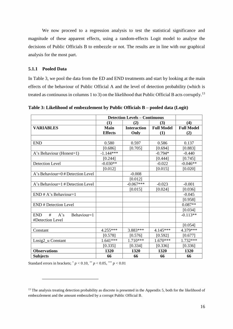
5.1.1 Pooled Data
In Table 3, we pool the data from the ED and END treatments and start by looking at the main
effects of the behaviour of Public Official A and the level of detection probability (which is
treated as continuous in columns 1 to 3) on the likelihood that Public Official B acts corruptly.13
Table 3: Likelihood of embezzlement by Public Officials B – pooled data (Logit)
Detection Levels – Continuous
(1) (2) (3) (4)
VARIABLES Main
Effects
Interaction
Only
Full Model
(1)
Full Model
(2)
END 0.580 0.597 0.586 0.137
[0.686] [0.705] [0.694] [0.883]
A’s Behaviour (Honest=1) -1.144*** -0.794* -0.440
[0.244] [0.444] [0.745]
Detection Level -0.030** -0.022 -0.046**
[0.012] [0.015] [0.020]
A’s Behaviour=0 # Detection Level -0.008
[0.012]
A’s Behaviour=1 # Detection Level -0.067*** -0.023 -0.001
[0.015] [0.024] [0.036]
END # A’s Behaviour=1 -0.045
[0.958]
END # Detection Level 0.087**
[0.034]
END # A’s Behaviour=1
#Detection Level
-0.113**
[0.054]
Constant 4.255*** 3.883*** 4.145*** 4.379***
[0.578] [0.576] [0.592] [0.677]
Lnsig2_u Constant 1.641*** 1.710*** 1.670*** 1.732***
[0.335] [0.334] [0.336] [0.336]
Observations 1320 1320 1320 1320
Subjects 66 66 66 66
Standard errors in brackets; * p < 0.10, ** p < 0.05, *** p < 0.01
13 The analysis treating detection probability as discrete is presented in the Appendix 5, both for the likelihood of
embezzlement and the amount embezzled by a corrupt Public Official B.

17
In column 1, we include only the main effects in the regression (Equation 1) and find a
significant and negative relationship between honest behaviour by Public Official A and the
likelihood of embezzlement by Public Official B (at the 1 per cent level). We also find that
deterrence has a negative and statistically significant effect on the likelihood that Public
Official B acts corruptly. This deterrence effect is in line with much of the experimental
literature outlined above. Our pooled data thus suggests the presence of a contagion effect and
of a deterrence effect.
The regression framework allows us to go deeper and study the interaction of Public
Official A’s behaviour and the level of detection that he/she chooses. In column 2 of Table 3
(corresponding to Equation 2), we include only interaction terms between Public Official A’s
behaviour and the level of detection.14 The level of detection has no effect on the likelihood
that Public Official B acts corruptly when chosen by a corrupt Public Official A. In contrast,
when chosen by an honest Public Official A, a greater chance of detection significantly
decreases the likelihood of embezzlement by Public Official B (at the 1 per cent level). The
difference between the coefficients for each type of Public Official A is significant at the 1 per
cent level (p-value = 0.000, chi2). This is consistent with a legitimacy effect.
Column 3 of Table 3 includes the main effects and the interaction effect (Equation 3).
The reference group is a Public Official B in the ED treatment who is paired with a corrupt
Public Official A who has selected a zero probability of detection. The coefficient
for ‘detection level’ is negative suggesting that detection is effective when chosen by an honest
Public Official A but the effect is not significant at traditional levels. The coefficient for the
dummy representing an honest Public Official A is negative (and significant at the 10 per cent
level) indicating that the likelihood of embezzlement by Public Official B is higher when facing
a corrupt Public Official A instead of an honest Public Official A. Graphically, this would mean
that the line of predicted Logit values for corrupt Public Officials A will lie above the line for
their honest counterparts.
14 In column 2 of Table 3 (Interaction only), we have two continuous variables (CorruptA*Detection and
HonestA*Detection) as detection is treated as a continuous variable. The standard interpretation of the constant
in a regression equation is the expected mean value of Y (dependent variable) when all other explanatory variables
are 0. ‘CorruptA*Detection’ and ‘HonestA*Detection’ are simultaneously 0 when detection = 0 for either type of
public official A. As a result, the constant does not represent a specific reference group but a mean for corrupt and
honest A when detection is 0. The same applies to columns 3 and 4 in Table 5, column 2 in Table 8, and columns
3 and 4 of Table 6.

18
It is important to note that in presence of an interaction term, the statistical significance
of the main effects and the interaction term do not tell much about the interactive effect
(Brambor et al. 2006), especially when one of the interaction variables is continuous. Indeed,
at first sight, the insignificant interaction term in column 3 of Table 3 might seem to suggest
that the marginal effect of Public Official A’s behaviour does not depend on the level of
detection. However, the marginal effects of Public Official A’s type may be significantly
different for different detection levels. Indeed, note that the coefficient for ‘A’s behaviour’ in
column 3 gives the overall effect of an Honest A when ‘detection level’ equals 0. Since
detection level is a continuous variable, it takes many values other than 0. To understand the
overall effects of ‘A’s behaviour’ on embezzlement, we plug in different values of Detection
Level into Equation 3 (column 3 in Table 3). This allows us to see, for each level of detection,
how the likelihood of embezzlement (the dependent variable) changes depending on Public
Official A’s type (corrupt or honest). Column 1 of Table 4 presents the results on the
differences in the overall average marginal effects between corrupt and honest Officials A.
They suggest that the probability of embezzlement by Public Official B is significantly higher
when paired with a corrupt Public Official A than with an honest Public Official A, at all levels
of detection.15 That is to say that the same policy yields different results depending on the
behaviour of the policy maker. This is consistent with the results presented in column 2 of
Table 3. The models in columns 2 and 3 of Table 3 thus also provide evidence that legitimacy
matters for the effectiveness of deterrence as anti-corruption policy.
In column 4 of Table 3, we run a three-way interaction between the END treatment,
Public Official A’s type, and detection levels. The main objective is to see if there are
differences between the ED and the END treatments. The results suggest that while detection
has a negative and significant effect on the likelihood of embezzlement (see ‘Detection Level’
coefficient), its impact is lower in the END treatment compared to the ED treatment (see ‘END
# Detection Level’ coefficient). There is also a significant difference in the impact of detection
when chosen by an honest Official A (compared to a corrupt Official A) in the END treatment
(see ‘END # A’s Behaviour=1 #Detection Level’ coefficient); while such a difference in not
found in the ED treatment (see ‘A’s Behaviour=1 #Detection Level’ coefficient). To further
15 The difference in marginal effects is: ‘Marginal Effect of Honest A’ – ‘Marginal Effect of Corrupt A’.
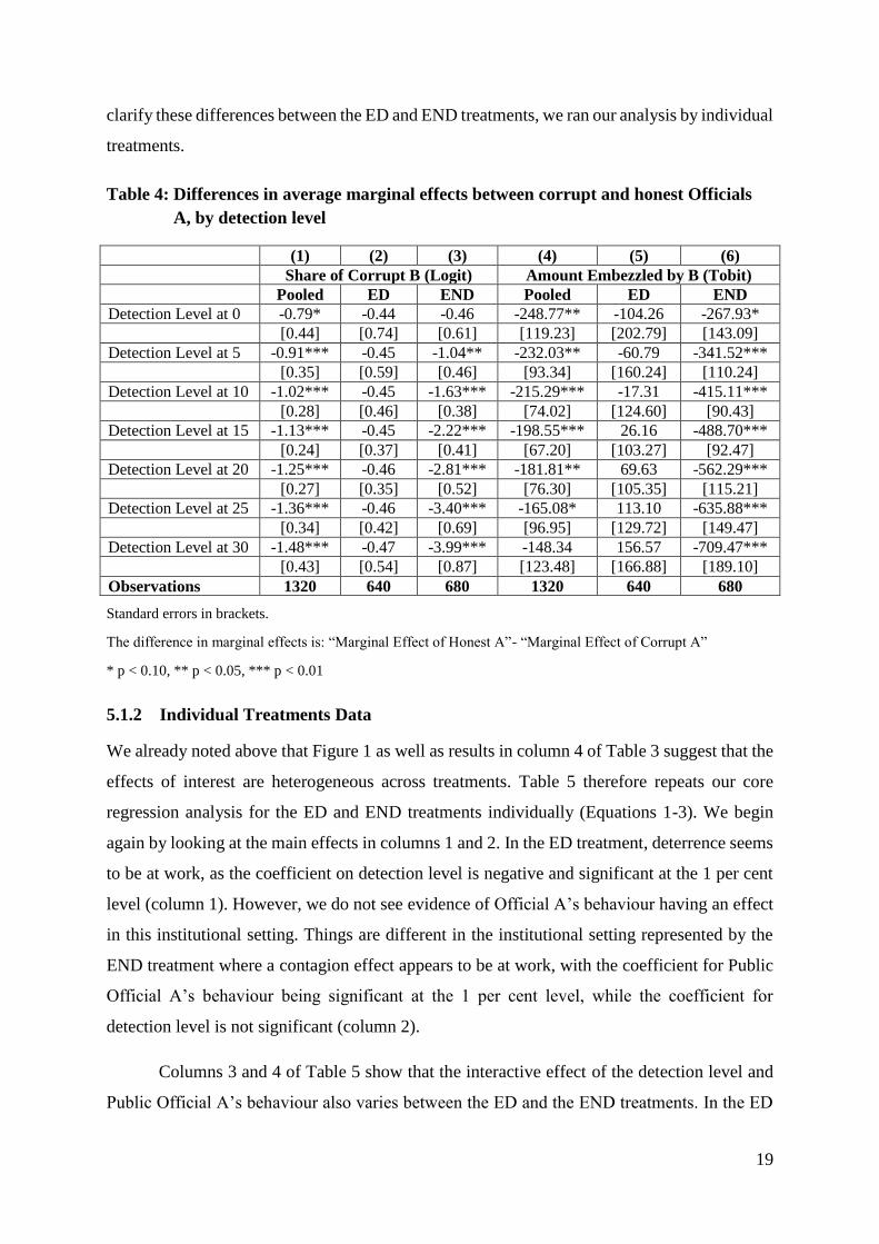
19
clarify these differences between the ED and END treatments, we ran our analysis by individual
treatments.
Table 4: Differences in average marginal effects between corrupt and honest Officials
A, by detection level
(1) (2) (3) (4) (5) (6)
Share of Corrupt B (Logit) Amount Embezzled by B (Tobit)
Pooled ED END Pooled ED END
Detection Level at 0 -0.79* -0.44 -0.46 -248.77** -104.26 -267.93*
[0.44] [0.74] [0.61] [119.23] [202.79] [143.09]
Detection Level at 5 -0.91*** -0.45 -1.04** -232.03** -60.79 -341.52***
[0.35] [0.59] [0.46] [93.34] [160.24] [110.24]
Detection Level at 10 -1.02*** -0.45 -1.63*** -215.29*** -17.31 -415.11***
[0.28] [0.46] [0.38] [74.02] [124.60] [90.43]
Detection Level at 15 -1.13*** -0.45 -2.22*** -198.55*** 26.16 -488.70***
[0.24] [0.37] [0.41] [67.20] [103.27] [92.47]
Detection Level at 20 -1.25*** -0.46 -2.81*** -181.81** 69.63 -562.29***
[0.27] [0.35] [0.52] [76.30] [105.35] [115.21]
Detection Level at 25 -1.36*** -0.46 -3.40*** -165.08* 113.10 -635.88***
[0.34] [0.42] [0.69] [96.95] [129.72] [149.47]
Detection Level at 30 -1.48*** -0.47 -3.99*** -148.34 156.57 -709.47***
[0.43] [0.54] [0.87] [123.48] [166.88] [189.10]
Observations 1320 640 680 1320 640 680
Standard errors in brackets.
The difference in marginal effects is: “Marginal Effect of Honest A”- “Marginal Effect of Corrupt A”
* p < 0.10, ** p < 0.05, *** p < 0.01
5.1.2 Individual Treatments Data
We already noted above that Figure 1 as well as results in column 4 of Table 3 suggest that the
effects of interest are heterogeneous across treatments. Table 5 therefore repeats our core
regression analysis for the ED and END treatments individually (Equations 1-3). We begin
again by looking at the main effects in columns 1 and 2. In the ED treatment, deterrence seems
to be at work, as the coefficient on detection level is negative and significant at the 1 per cent
level (column 1). However, we do not see evidence of Official A’s behaviour having an effect
in this institutional setting. Things are different in the institutional setting represented by the
END treatment where a contagion effect appears to be at work, with the coefficient for Public
Official A’s behaviour being significant at the 1 per cent level, while the coefficient for
detection level is not significant (column 2).
Columns 3 and 4 of Table 5 show that the interactive effect of the detection level and
Public Official A’s behaviour also varies between the ED and the END treatments. In the ED
20
treatment, detection and punishment significantly decreases the likelihood of Public Official B
being corrupt when chosen by a corrupt Public Official A. Likewise, there is a significant
negative effect when the level of detection is chosen by an honest Public Official A.
Table 5.1: Detection levels – dummy
Likelihood of Embezzlement
(Logit)
Amount Embezzled (Tobit)
(1) (2) (3) (4)
VARIABLES Main Effects Interaction
Only
Main
Effects
Interaction
Only
END 0.599 0.615 22.636 44.585
[0.698] [0.713] [192.130] [192.371]
A’s Behaviour (Honest=1) -1.191*** -191.624***
[0.249] [67.339]
Detection Level
A’s Behaviour=0 # Detection
Level
A’s Behaviour=1 # Detection
Level
Detection Level=5 -0.512 -304.588***
[0.470] [100.041]
Detection Level=10 -0.698 -363.048***
[0.477] [109.614]
Detection Level=15 -0.765* -397.836***
[0.451] [110.310]
Detection Level=20 -0.983** -404.543***
[0.443] [100.895]
Detection Level=25 -0.438 -255.449**
[0.474] [114.025]
Detection Level=30 -1.273*** -428.595***
[0.435] [103.949]
A’s Behaviour=0 # Detection
Level=5
-0.393 -257.555**
[0.622] [113.599]
A’s Behaviour=0 # Detection
Level=10
-0.690 -263.998**
[0.603] [126.544]
A’s Behaviour=0 # Detection
Level=15
-0.461 -247.005*
[0.614] [131.626]
A’s Behaviour=0 # Detection
Level=20
-0.815 -383.438***
[0.549] [111.624]
A’s Behaviour=0 # Detection
Level=25
-0.230 -275.637**
[0.631] [132.903]

21
Likelihood of Embezzlement
(Logit)
Amount Embezzled (Tobit)
(1) (2) (3) (4)
VARIABLES Main Effects Interaction
Only
Main
Effects
Interaction
Only
A’s Behaviour=0 # Detection
Level=30
-0.900* -386.808***
[0.542] [118.230]
A’s Behaviour=1 # Detection
Level=0
-0.763 1.250
[0.667] [172.500]
A’s Behaviour=1 # Detection
Level=5
-1.471** -481.615***
[0.636] [156.820]
A’s Behaviour=1 # Detection
Level=10
-1.379* -657.058***
[0.735] [177.086]
A’s Behaviour=1 # Detection
Level=15
-1.867*** -760.104***
[0.635] [166.469]
A’s Behaviour=1 # Detection
Level=20
-1.950*** -464.827***
[0.681] [167.930]
A’s Behaviour=1 # Detection
Level=25
-1.430** -271.534
[0.677] [176.402]
A’s Behaviour=1 # Detection
Level=30
-2.812*** -575.989***
[0.701] [180.288]
Constant 4.529*** 4.392*** 1973.808*** 1922.339***
[0.635] [0.688] [153.315] [157.141]
Lnsig2u Constant/ Sigma_u
Constant
1.670*** 1.721*** 737.499*** 737.578***
[0.335] [0.337] [72.029] [72.015]
Sigma_e Constant 942.282*** 939.372***
[26.175] [26.090]
Observations 1320 1320 1320 1320
Subjects 66 66 66 66
Standard errors in brackets; * p < 0.10, ** p < 0.05, *** p < 0.01
However, the difference in the marginal effect of the detection level by type of Public
Official A is not statistically significant (p-value = 0.238, chi2). In the END treatment,
however, detection and punishment appear to increase the likelihood of Public Official B being
corrupt when chosen by a corrupt Public Official A and this effect is statistically significant at
the 5 per cent level. In contrast, there is a significant negative effect when the probability of
detection is chosen by an honest Public Official A. The difference in the effect of the detection
level chosen by corrupt or honest Public Official As is significant at the 1 per cent level (p-
value = 0.000, chi2). Such a result suggests that, under certain conditions, an anti-corruption

22
policy based on detection and punishment can be counter-productive when chosen by a policy
maker who is herself corrupt.
The full model presented in column 5 of Table 5 shows that Official A’s behaviour has
no significant effect on Official B’s likelihood to embezzle in the ED treatment but that there
is a deterrence effect. Table 4, column 2, further confirms that there is no significant effect of
Public Official A’s type at any detection level. Thus, we conclude that in the particular
institutional framework captured by the ED treatment, monitoring and punishment are effective
and the behaviour of the rule maker is irrelevant. These conclusions are in line with the
graphical analysis in Figure 1 and the findings of the literature on exogenously given detection
levels that began with Abbink et al. (2002).
In the END treatment (Table 5, column 6), we find no evidence of Official A’s
behaviour affecting that of Official B and we can also see that detection levels chosen by a
corrupt Public Official A have no significant effect on the likelihood of embezzlement by
Public Official B. However, the negative and significant interaction term suggests that choices
made by honest Public Officials A tend to decrease the likelihood of embezzlement by Public
Official B. This is consistent with the idea of a legitimacy effect. Once again, these conclusions
are fully consistent with the graphical analysis presented in Figure 1. They are also confirmed
in Table 4, column 3. Public Official B embezzles with a significantly higher probability (at
conventional 1 per cent or 5 per cent levels), when facing a corrupt rather than an honest Public
Official A, at all non-zero levels of detection.
Our results thus indicate that in the END treatment, a higher probability of detection
and punishment can effectively deter corruption, but only when the policy is put in place by a
policy maker who is himself ‘clean’. Thus, in institutional settings in which equality before the
law is observed, it is vital that those at the top set the right ‘tone’, if endogenously chosen anti-
corruption measures of this type are to be effective.
5.1.3 Robustness Check
Given that we find a legitimacy effect only in the END treatment, we focus our robustness
check on this treatment by comparing it with the XND treatment. We only consider END data
points where 30 per cent was chosen. As a result, the only difference between these two
treatments is that the detection probability is chosen by Public Official A in the END treatment,
while it is exogenously set at 30 per cent in the XND treatment. The idea is to check whether
23
Public Official A’s behaviour has an impact on the effectiveness of her detection choices,
focusing on the highest detection level available.
When the detection probability is 30 per cent, the average shares of corrupt decisions
are 89 per cent and 79 per cent in the END and XND treatments respectively. The results in
Table 6 (column 1) suggest a significantly higher likelihood of embezzlement by corrupt
Officials B in the END treatment, compared to the XND treatment. In the XND treatment
where detection is set exogenously, we find no significant difference in the likelihood of
embezzlement by Public Official B, when facing a corrupt or an honest Public Official A (see
coefficient for ‘A’s Behaviour (Honest=1)’ in Table 6, column 1). In contrast, in the END
treatment, we find that facing an honest Public Official A significantly decreases the likelihood
of embezzlement by Public Official B at the 1 per cent level (see coefficient for ‘END # A’s
Behaviour=1’ in Table 6, column 1). In other words, choosing the highest level of detection
available in our setting increases (decreases) the likelihood of embezzlement when the decision
maker is corrupt (honest), compared to a situation where this level of detection is set
exogenously. Such a result shows an interaction between Public Official A’s behaviour and
his/her detection choices further confirming the existence of a legitimacy effect.
Table 6: Likelihood and amount embezzled by Public Officials B
Detection Level 30
Likelihood of Embezzlement
(Logit)
Amount Embezzled
(Tobit)
Baseline Group: Corrupt Official B in XND
END 3.286** 628.545*
[1.502] [345.969]
A’s Behaviour (Honest=1) 0.035 -105.231
[0.285] [84.955]
END # A’s Behaviour=1 -4.339*** -576.770
[1.668] [361.151]
Constant 2.636*** 1231.104***
[0.580] [207.894]
Lnsig2u/Sigma_u Constant 2.111*** 1147.022***
[0.385] [134.398]
Sigma_e Constant
924.418***
Observations 724 724
Subjects 62 62
Standard errors in brackets:* p < 0.10, ** p < 0.05, *** p < 0.01.
24
5.2 Amount Embezzled by Public Officials B
Next we analyse the amount embezzled by Public Official B. Especially in contexts where
some level of corruption is expected, the factors outlined above could operate on the decision
regarding the extent of corruption as well as the decision to be corrupt or not. That is to say
that the tone at the top could lead to people embezzling more or less even though the probability
of detection and punishment is the same no matter the level of their embezzlement. The analysis
here mirrors the one conducted in Section 5.1. The amounts kept by Public Official B in the
ED, END, and XND treatments are respectively 1,488ECU, 1,494ECU, and 1,199ECU (see
Table 3). Relative to the XND treatment, we find that the amounts embezzled increase
significantly both in the ED and END treatments at the 10 per cent significance level (p-value
= 0.09 for both, two-sided Mann-Whitney). No significant difference is found between the ED
and END treatments (p-value = 0.76, Mann-Whitney).
We now proceed to disaggregate the amount embezzled by Officials B according to
Public Official A’s behaviour (honest or corrupt) and the detection level chosen by Public
Official A. Figure 2 carries out the same exercise as Figure 1, for the extent of Public Official
B’s embezzlement. Once again, it should be noted that since, for a given probability of
detection, embezzling 1ECU is as likely to result in punishment as embezzling 2,280ECU, it is
not obvious that higher probabilities should lead to an individual embezzling a lower amount.
However, we observe a negative relationship between the level of detection and the amount
embezzled in the pooled data and in the ED treatment. Such evidence of deterrence is observed
whether Public Official A is corrupt or honest. The pooled data picture is consistent with a
contagion effect and a legitimacy effect, though once again these effects appear to be
unimportant in the ED treatment. The END treatment also shows a contagion effect and a
legitimacy effect in that each endogenously chosen level of detection probability (with the
possible exception of the 25 per cent level) gives rise to a lower average amount embezzled
when chosen by an honest as opposed to a corrupt Public Official A. For both types, we see
some evidence of a deterrence effect of monitoring and punishment.
Next we verify that the broad patterns observed in Figure 2 are statistically significant
using regression analysis. The results confirm our graphical analysis for the most part.

25
5.2.1 Pooled Data
In Table 7, we pool the data from the ED and END treatments and start in column 1 by looking
at the main effects of Public Official A’s behaviour and of the probability of detection on the
amount embezzled (Equation 1). Our regression shows a statistically significant and negative
relationship between the detection level and the amount embezzled by Public Official B (at the
1 per cent level). The magnitude of this deterrence effect is a roughly 11ECU decrease in
embezzlement per additional 1 per cent probability of detection. There is also evidence of a
contagion effect as the coefficient on the dummy variable capturing an honest Public Official
A is significant and negative. This magnitude of this effect is also meaningful. When facing a
corrupt Public Official A, Public Official B embezzles an additional 200ECU on average.
Table 7: Amount embezzled by Public Officials B – pooled data (Tobit)
Detection Levels – Continuous
(1) (2) (3) (4)
VARIABLES Main
Effects
Interaction
Only
Full Model
(1)
Full Model
(2)
END 9.813 13.163 8.726 -116.269
[190.606] [191.213] [190.567] [216.652]
A’s Behaviour (Honest=1) -199.841*** -248.772** -96.368
[67.160] [119.227] [187.562]
Detection Level -10.807*** -11.613*** -19.319***
[3.035] [3.442] [5.021]
A’s Behaviour=0 # Detection
Level
-8.718***
[3.150]
A’s Behaviour=1 # Detection
Level
-17.004*** 3.348 8.343
[4.245] [6.738] [9.519]
END # A’s Behaviour=1 -184.404
[242.776]
END # Detection Level 18.790***
[6.929]
END # A’s Behaviour=1
#Detection Level
-23.518*
[13.857]
Constant 1842.657*** 1791.507*** 1854.575*** 1925.989***
[147.004] [146.195] [148.937] [163.269]
Lnsig2_u Constant 734.325*** 736.813*** 734.115*** 728.815***
[71.838] [72.048] [71.822] [71.275]
Lnsig2_e Constant 947.854*** 949.125*** 947.769*** 938.923***
[26.344] [26.384] [26.341] [26.083]
Observations 1320 1320 1320 1320
Subjects 66 66 66 66
Standard errors in brackets;* p < 0.10, ** p < 0.05, *** p < 0.01
26
In Table 7, column 2, we include only the interaction terms between Public Official A’s
behaviour and detection (Equation 2). We find that the decision made by Public Official A (to
be corrupt or honest) has an effect on the amount embezzled by Public Official B. While
detection decreases the amount embezzled regardless of whether it was chosen by a corrupt or
an honest Public Official A, we find that the effects of detection levels chosen by an honest
Public Official A (coefficient of -17.0) are almost double those of detection probabilities
chosen by a corrupt Public Official A (coefficient of -8.7). This difference is significant at the
5 per cent level (p-value = 0.0293, chi2) thereby suggesting a legitimacy effect.
The results of the full model (including the main effects and interaction term) are shown
in column 3 of Table 7. Here the baseline group is a Public Official B in the ED treatment
encountering a corrupt Public Official A who has chosen detection level 0. The coefficient
on the level of detection is negatively signed and statistically significant at the 1 per cent level.
The coefficient on Public Official A’s behaviour is negative and significant at the 5 per cent
level, suggesting that on average Public Officials B embezzle a lower amount when facing
honest Public Officials A. To see whether the effects for honest and corrupt Public Officials A
are significantly different at different detection levels, we compute the difference in the average
marginal effect of type by detection level of Public Officials A. The results, which are presented
in Table 4, column 4, suggest that facing a corrupt Public Official A rather than an honest one
significantly increases the amount embezzled by Public Official B at all levels of detection
except the highest one (i.e. 30 per cent).
In column 4 of Table 7, we run again a three-way interaction between the END
treatment, Public Official A’s type and detection levels. We find that there are differences
between the ED and the END treatments. Indeed, while detection has a negative and significant
effect on the amount embezzled (see ‘Detection Level’ coefficient), its impact is lower in the
END treatment compared to the ED treatment (see ‘END # Detection Level’ coefficient). There
is also a significant difference in the impact of detection when chosen by an honest Official A
(compared to a corrupt Official A) in the END treatment (see ‘END # A’s Behaviour=1
#Detection Level’ coefficient); but not in the ED treatment (see ‘A’s Behaviour=1 #Detection
Level’ coefficient). Thus, we next run our analysis by individual treatments to further explore
the differences between the ED and END treatments.

27
5.2.2 Individual Treatments Data
Table 8 shows that the effects observed for the average amount of embezzlement vary
depending on the treatment. That is to say that the institutional framework, specifically the
presence of procedural equality before the law, determines the importance of deterrence, and
legitimacy effects. We begin by looking at the main effects (Equation 1). Column 1 of Table 8
tells us that in the ED treatment, where equality before the law is not observed, there is a
deterrence effect as the coefficient for detection level is negative and significant at the 1 per
cent level. However, the coefficient on Public Official A’s behaviour is not significant, leaving
us with no clear evidence of a contagion effect. Both of these conclusions are in line with Figure
2. The situation in the END treatment is quite the opposite in that in column 2 of Table 8, we
find evidence of a contagion effect, with the coefficient for behaviour of Public Officials A
being significant at the 1 per cent level, while the coefficient for deterrence is not significant.
Table 8: Amount embezzled by Public Officials B, by treatment (Tobit) Main Effects Interaction Only Full Model
(1) (2) (3) (4) (5) (6)
VARIABLES ED END ED END ED END
A’s Behaviour
(Honest=1)
44.371 -446.445*** -104.255 -267.928*
[101.064] [88.443] [202.787] [143.088]
Detection
Level
-18.028*** -3.923 -20.312*** -0.535
[4.713] [3.881] [5.442] [4.429]
A’s
Behaviour=0
# Detection
Level
-19.024*** 2.584
[4.824] [4.117]
A’s
Behaviour=1
# Detection
Level
-14.916** -25.947*** 8.694 -14.718
[6.201] [5.892] [10.289] [9.325]
Constant 1915.492*** 1829.088*** 1926.186*** 1733.262*** 1955.257*** 1792.272***
[149.184] [149.398] [145.967] [148.680] [156.716] [151.246]
Sigma_u
Constant
636.315*** 796.107*** 636.778*** 802.957*** 636.972*** 797.464***
[92.486] [106.146] [92.542] [106.895] [92.572] [106.260]
Sigma_e
Constant
1016.112*** 871.252*** 1015.675*** 872.039*** 1015.717*** 869.630***
Observations [41.540] [32.969] [41.518] [33.006] [41.521] [32.906]
Subjects 640 680 640 680 640 680
Standard errors in brackets; * p < 0.10, ** p < 0.05, *** p < 0.01
28
We also see differences between the ED and the END treatments when looking at the
effect of detection probability according to Public Official A’s type (Equation 2). In the ED
treatment, a higher likelihood of detection significantly decreases the amount embezzled by
Public Officials B on average regardless of whether Public Officials A are corrupt or honest
(Table 8, column 3). Furthermore, the difference in the coefficients is not significant at
conventional levels (p-value = 0.4228, chi2). Table 8, column 4 tells us that in the END
treatment the level of detection has no effect on the amount embezzled when that level has
been enacted by corrupt Public Officials A. However, anti-corruption laws enacted by honest
Public Officials A do decrease the amount embezzled by Public Officials B significantly at the
1 per cent level. This difference between the effectiveness of policies promulgated by corrupt
and honest Public Officials A is significant at the 1 per cent level (p-value = 0.000, chi2). We
take this as evidence of a legitimacy effect in the amount embezzled.
The full model (Equation 3) for the ED treatment in Table 8, column 5 shows no
significant contagion effect but again indicates the presence of a deterrence effect. Table 4,
column 5, further confirms that there are no significant differences in the average marginal
effects of the type of Public Officials A at specific detection level. The full model for the END
treatment (Table 8, column 6) finds evidence for a contagion effect at the 10 per cent level of
significance and no evidence of a simple deterrence effect. The interaction term is negative but
not statistically significant. Table 4, column 6 shows that changing Public Official A’s type
from corrupt to honest would lead Public Official B to embezzle a lower amount of funds at all
levels of detection.
5.2.3 Robustness Check
In this section, we reproduce the same exercise as in Section 5.1.3 by comparing the XND and
END treatment at detection level 30; except that the variable of interest is the amount
embezzled. When the detection probability is 30 per cent the average amounts embezzled are
1,488ECU and 1,198ECU in the END and XND treatments respectively.
The results are shown in Table 6 (column 2). They suggest a significantly higher amount
of embezzlement by corrupt Officials B in the END treatment (at the 10 per cent level),
compared to the XND treatment. In the XND treatment where detection is set exogenously, we
find no significant difference in the amount embezzled by Public Officials B, when facing a
corrupt or an honest Public Official A (see coefficient for ‘A’s Behaviour (Honest=1)’ in Table

29
6, column 2). Likewise, in the END treatment, we find that facing an honest Public Official A
does not have a significant effect on the amount embezzled by Public Officials B (see
coefficient for ‘END # A’s Behaviour=1’ in Table 6, column 2); despite the coefficient having
the expected sign. The weaker result found relative to the amount embezzled may be explained
by the fact that, for a given probability of detection in our experiment, embezzling 1ECU is as
likely to result in punishment as embezzling 2,280ECU, making the choice of amount less
dependant on the probability of detection.
6 Concluding Remarks
This paper draws on data obtained from a framed laboratory experiment carried out in Kenya
to examine the roles of contagion effects, deterrence effects, and legitimacy effects in the fight
against corruption. In our regression analysis, we labelled the main effect of the behaviour of
Public Officials A as a contagion effect, and that of the detection level as a deterrence effect.
The legitimacy effect refers to the interaction between As’ behaviour and detection levels. This
captured the idea that deterrence can be less effective when chosen by corrupt Public Officials
A.
Crucially, we found that the importance of these effects depended on the institutional
framework in which our ‘public officials’ are operating. When policy makers are exempt from
their own laws we find that a strong deterrence effect, a greater chance of being detected and
punished, reduces the likelihood and the extent of corruption. This effect does not depend on
the behaviour of the policy maker. In settings in which equality before the law is observed and
policy makers are liable to be caught in their own net, we find that detection policies are only
an effective deterrent when promulgated by honest policy makers. This legitimacy effect is
evident alongside a simple contagion effect. We also found that externally imposed rules may
be superior to equally stringent rules originating from a corrupt internal policy maker. Once
again, this existence of this effect was dependent on the internal policy maker being subject to
the provisions of the policy.
Our findings offer several important implications in fighting corruption for policy
makers and other interested parties – subject to the usual external validity caveats of
experimental economics which we will address briefly below. Firstly, our results add further
evidence as to the potential for detection and punishment mechanisms to play a role in curbing
corruption. Our findings of a contagion effect suggest that creating a culture of honesty among
the top-rank officials in systems such as the one in our experiment can have knock-on, or

30
perhaps trickle-down, effects on others within the organization or society (Moxnes and Van
der Heijden 2003; Güth et al. 2007; Levati et al. 2007; Cappelen et al. 2016). Our finding of a
strong legitimacy effect adds more weight to this argument in that fostering such an honest
ethic may result in the same policy being more effective. Moreover, internally generated anti-
corruption detection mechanisms will only be effective in institutional settings with equality
before the law when the policy maker is honest. If this condition is not met, exogenously
imposed rules are preferable.
The results on the effects of institutional settings on legitimacy can be related to the
perceived procedural fairness of the system. Indeed, the procedural fairness literature suggests
that legitimacy springs from a shared perception between all relevant parties and outsiders
about the fairness of the procedures applied – though outcomes may be unequal, at least
everyone acts under a common set of rules that equally apply to all (Lind 2001; Tyler 2004).
Perceived procedural fairness promotes compliance with the verdicts of the authority. Since
the seminal work of Thibault and Walker (1975), various studies have come to establish and
support these views (see e.g. Lind 2001; Falk et al. 2003; Tyler 2004; Bolton et al. 2005).
Therefore, it is somewhat surprising that in our setting, the asymmetric rules of the game
promote compliance independent of the behaviour of the authority that decides upon the anti-
corruption measures. Another potential explanation may relate to risk-taking behaviour in-
group vs individually; with several experiments suggesting that higher risk-taking behaviour
in groups compared to isolated individuals (for example, Yechiam et al. 2008; Lahno and Serra-
Garcia 2015). As detection applies to both officials in the END treatment, this may create a
group effect when Public Official A decides to embezzle despite setting a positive detection
level and despite the fact that in our detection mechanism, independent draws are carried out
for Officials A and B. In the ED treatment, no such effect exists as deterrence applies only to
Public Official B. Finally, perhaps the explanation for our results lies in the fact that the
ultimate authority that chooses the symmetric or asymmetric rules is not the first-moving
official but the experimenter. Given the importance of the institutional framework in our
results, future research could usefully endogenize the choice of whether the fight against
corruption applies to all and whether immunity is granted only to the top level, which has an
influence on the anti-corruption institutions.
As for the applicability of our lab results to the ‘real world’, a few arguments can be
noted. Firstly, while the magnitude of any given effect may not carry over from the lab to the
field, for an experiment to be useful we need only qualitative external validity (Camerer 2014;

31
Kessler and Vesterlund 2014). Secondly, external validity problems are not unique to
experimental results (Falk and Heckman 2009; Kessler and Vesterlund 2014). Finally, the very
nature of corruption makes data difficult to collect and means that there are practical and ethical
challenges to evaluating anti-corruption policies and institutions in a field setting (Armantier
and Boly 2012). Laboratory studies allow us to get a handle on what might work in a low-cost
and ethically feasible setting (Dusek et al. 2005; Abbink 2006).
References
Abbink, K. (2006) ‘Laboratory Experiments on Corruption’, in S. Rose-Ackerman (ed.) The
Handbook of Corruption, Cheltenham, UK and Northampton, MA: Edward Elgar Publishers.
Abbink, K., Irlenbusch, B., and Renner, E. (2002) ‘An Experimental Bribery Game’, Journal
of Law, Economics, and Organization, Vol. 18, No. 2, pp. 428-54.
Abbink, K. and D. Serra (2012) ‘Anticorruption Policies: Lessons from the Lab’, Research in
Experimental Economics, Vol. 15, pp. 77-115.
Akerlof, R. (2016) ‘The Importance of Legitimacy’, The World Bank Economic Review, Vol.
30, Supplement 1, pp. S157-S165.
Armantier, O. and Boly, A. (2012) ‘On the External Validity of Laboratory Experiments on
Corruption’, in D. Serra and L. Wantchekon (eds) New Advances in Experimental Research on
Corruption, Research in Experimental Economics series, Vol. 15, pp. 117-44. Bingley, UK:
Emerald Group Publishing.
Azfar, O. and Nelson, W.R., Jr (2007) ‘Transparency, Wages, and the Separation of Powers:
An Experimental Analysis of Corruption’, Public Choice, Vol. 130, Nos 3-4, pp. 471-93.
Bandiera, O., Barankay, I., and Rasul, I. (2010) ‘Social Incentives in the Workplace’, Review
of Economic Studies, Vol. 77, No. 2, pp. 417-58.
Barr, A., Lindelow, M., and Serneels, P. (2009) ‘Corruption in Public Service Delivery: An
Experimental Analysis’, Journal of Economic Behavior & Organization, Vol. 72, No. 1,
pp. 225-39.
Basu, K. (2015) ‘The Republic of Beliefs: A New Approach to Law and Economics’, World
Bank Policy Research Working Paper 7259, Washington, D.C.: World Bank.
Beams, J.D., Brown, R.M., and Killough, L.N. (2003) ‘An Experiment Testing the
Determinants of Non-compliance with Insider Trading Laws’, Journal of Business Ethics, Vol.
45, No. 4, pp. 309-23.
Becker, G.S. (1968) ‘Crime and Punishment: An Economic Approach’, Journal of Political
Economy, Vol. 76, No. 2, 169-217.
Bikhchandani, S., Hirshleifer, D., and Welch, I. (1998), ‘Learning from the Behavior of Others:
Conformity, Fads, and Informational Cascades’, The Journal of Economic Perspectives, Vol.
12, No. 3, pp. 151-70.

32
Bolton, G.E., Brandts, J., and Ockenfels, A. (2005) ‘Fair Procedures: Evidence from Games
Involving Lotteries’, Economic Journal, Vol. 115, No. 506, pp. 1054-76.
Boly, A. and Gillanders, R. (2016) ‘Anti-corruption Policy-making, Discretionary Power, and
Institutional Quality’, UNU-WIDER Working Paper No. 2016/88, Helsinki: UNU-WIDER.
Brambor, T., Clark, W.R., and Golder, M. (2006) ‘Understanding Interaction Models:
Improving Empirical Analyses’, Political Analysis, Vol. 14, pp. 63-82.
Brandts, J. and A. Schram (2001) ‘Cooperation and Noise in Public Goods Experiments:
Applying the Contribution Function Approach’, Journal of Public Economics, Vol. 79, No. 2,
pp. 399-427.
Camerer, C.F. (2014) ‘The Promise and Success of Lab-Field Generalizability in Experimental
Economics: A Reply to Levitt and List’, in G. Fréchette and A. Schotter (eds) The Methods of
Modern Experimental Economics, Oxford: Oxford University Press.
Cappelen, A.W., Reme, B.-A., Sørensen, E.Ø., and Tungodden, B. (2016) ‘Leadership and
Incentives’, Management Science, Vol. 62, No. 7, pp. 1944-53.
Chen, D. (2013) ‘The Deterrent Effect of the Death Penalty? Evidence from British
Commutations during World War I’, NBER Working Paper, Cambridge, MA: National Bureau
of Economic Research.
d’Adda, G., Darai, D., and Weber, R.A. (2014) ‘Do Leaders Affect Ethical Conduct?’ Working
Paper No. 167, Zurich: University of Zurich.
Dusek, L., Ortmann, A., and Lizal, L. (2005) ‘Understanding Corruption and Corruptibility
through Experiments: A Primer’, Prague Economic Papers, Vol. 14, 2, pp. 147-62.
Eide, E., Rubin, P.H., and Shepherd, J.M. (2006) Economics of Crime, Boston, MA: Now
Publishers.
Falk, A. and Heckman, J.J. (2009) ‘Lab Experiments Are a Major Source of Knowledge in the
Social Sciences’, Science, Vol. 326, pp. 535-38.
Falk, A. and Ichino, A. (2006) ‘Clean Evidence on Peer Effects’, Journal of Labor Economics,
Vol. 24, No. 1, pp. 39-57.
Falk, A. and Kosfeld, M. (2006) ‘The Hidden Costs of Control’, American Economic Review,
Vol. 96, No. 5, pp. 1611-30.
Falk, A., Fehr, E., and Fischbacher, U. (2003) ‘On the Nature of Fair Behavior’, Economic
Inquiry, Vol. 41, No. 1, pp. 20-26.
Fehr, E. and Rockenbach, B. (2003) ‘Detrimental Effects of Sanctions on Human Altruism’,
Nature, Vol. 422, No. 6928, pp. 137-40.
Fisman, R. and Svensson, J. (2007) ‘Are Corruption and Taxation Really Harmful to Growth?
Firm Level Evidence’, Journal of Development Economics, Vol. 83, No. 1,
pp. 63-75.

33
Fischbacher, U. and Gächter, S. (2010) ‘Social Preferences, Beliefs, and the Dynamics of Free
Riding in Public Goods Experiments’, American Economic Review, Vol. 100, No. 1, pp. 541-
56.
Fortin, B., Lacroix, G., and Villeval, M.C. (2007).‘Tax Evasion and Social Interactions’,
Journal of Public Economics, Vol. 91, No. 11, pp. 2089-112.
Francois, P. (2000) ‘“Public Service Motivation” as an Argument for Government Provision’,
Journal of Public Economics, Vol. 78, No. 3, pp. 275-99.
Francois, P. (2003) ‘Not-For-Profit Provision of Public Services’, Economic Journal, Vol. 113,
No. 486, pp. C53-C61.
Francken, N., Minten, B., and Swinnen, J.F. (2009) Media, Monitoring, and Capture of Public
Funds: Evidence from Madagascar, World Development, Vol. 37, No. 1, pp. 242-55.
Gauthier, B. and Wane, W. (2009) Leakage of Public Resources in the Health Sector: An
Empirical Investigation of Chad, Journal of African Economies, Vol. 18, No. 1, pp. 52-83.
Gupta, S., Davoodi, H., and Alonso-Terme, R. (2002) ‘Does Corruption Affect Income
Inequality and Poverty?’ Economics of Governance, Vol. 3, No. 1, pp. 23-45.
Güth, W., Levati, M.V., Sutter, M., and Van der Heijden. E. (2007) ‘Leading by Example with
and without Exclusion Power in Voluntary Contribution Experiments’. Journal of Public
Economics, Vol. 91, No. 5, pp. 1023-42.
Hanna, R., Bishop, S., Nadel, S., Scheffler, G., and Durlacher, K. (2011) ‘The Effectiveness of
Anti-corruption Policy: What Has Worked, What Hasn’t, and What We Don’t Know – a
Systematic Review’, EPPI-Centre Report, No. 1909, London: Institute of Education,
University of London.
Jones, G.E. and Kavanagh, M.J. (1996) ‘An Experimental Examination of the Effects of
Individual and Situational Factors on Unethical Behavioral Intentions in the Workplace’,
Journal of Business Ethics, Vol. 15, No. 5, pp. 511-23.
Kagan, R.A. and Scholz, J.T. (1984) ‘The Criminology of the Corporation and Regulatory
Enforcement Strategies’, in K. Hawkins and J.M. Thomas (eds) Enforcing Regulation, Boston
MA: Kluwer-Nijhoff.
Kessler, J.B. and Vesterlund, L. (2014) ‘The External Validity of Laboratory Experiments:
Qualitative rather than Quantitative Effects’, in G. Fréchette and A. Schotter (eds) The Methods
of Modern Experimental Economics, Oxford: Oxford University Press.
Keizer, K., Lindenberg, S., and Steg, L. (2008) ‘The Spreading of Disorder’ Science, Vol. 322,
No. 5908, pp. 1681-85.
Lambsdorff, J.G. (2015) ‘Preventing Corruption by Promoting Trust: Insights from Behavioral
Science’, Vol. 69, No. 15, Passauer Diskussionspapiere: Volkswirtschaftliche Reihe,
Universität Passau.
Lahno, A.M. and Serra-Garcia, M. (2015) ‘Peer Effects in Risk Taking: Envy or Conformity?’
Journal of Risk and Uncertainty, Vol. 50, No. 1, pp. 73-95.
34
Levati, M.V., Sutter, M., and Van der Heijden, E. (2007) ‘Leading by Example in a Public
Goods Experiment with Heterogeneity and Incomplete Information’, Journal of Conflict
Resolution, Vol. 51, No. 5, 793-818.
Levi, M. and Sacks, A. (2009) ‘Legitimating Beliefs: Sources and Indicators’, Regulation &
Governance, Vol. 3, No. 4, pp. 311-33.
Lind, E.A. (2001) ‘Fairness Heuristic Theory: Justice Judgments as Pivotal Cognitions in
Organizational Relations’, in J. Greenberg & R. Cropanzano (eds) Advances in Organizational
Justice, pp. 56-88, Stanford, CA: Stanford University Press.
Mauro, P. (1995) ‘Corruption and Growth’, Quarterly Journal of Economics, Vol. 110, No. 3,
681-712.
Moxnes, E. and Van der Heijden, E. (2003) ‘The Effect of Leadership in a Public Bad
Experiment’, Journal of Conflict Resolution, Vol. 47, No. 6, pp. 773-95.
Olken, B.A. (2007) ‘Monitoring Corruption: Evidence from a Field Experiment in Indonesia’,
Journal of Political Economy, Vol. 115, No. 2, pp. 200-49.
Papachristos, A.V., Meares, T.L., and Fagan, J. (2012) ‘Why Do Criminals Obey the Law? The
Influence of Legitimacy and Social Networks on Active Gun Offenders’, The Journal of
Criminal Law & Criminology, Vol. 102, No. 2, pp. 397-440.
Pierce, L. and Snyder, J. (2008) ‘Ethical Spillovers in Firms: Evidence from Vehicle Emissions
Testing’, Management Science, Vol. 54, No. 11, pp. 1891-1903.
Reinikka, R. and Svensson, J. (2004) ‘Local Capture: Evidence from a Central Government
Transfer Program in Uganda’, The Quarterly Journal of Economics, Vol. 119, No. 2,
pp. 679-705.
Schnellenbach, J. (2007) ‘Tax Morale and the Legitimacy of Economic Policy’, Homo
Oeconomicus, Vol. 24, No. 1, pp. 21-45.
Schulze, G.G. and Frank, B. (2003) ‘Deterrence versus Intrinsic Motivation: Experimental
Evidence on the Determinants of Corruptibility’, Economics of Governance, Vol. 4, No. 2, pp.
143-60.
Serra, D. (2012) ‘Combining Top-down and Bottom-up Accountability: Evidence from a
Bribery Experiment’, Journal of Law, Economics, and Organization, Vol. 28, No. 3,
pp. 569-87.
Shang, J. and Croson, R. (2009) ‘A Field Experiment in Charitable Contribution: The Impact
of Social Information on the Voluntary Provision of Public Goods’, Economic Journal,
Vol. 119, No. 540, pp. 1422-39.
Smith, S., Windmeijer, F., and Wright, E. (2015) ‘Peer Effects in Charitable Giving: Evidence
from the (Running) Field’, Economic Journal, Vol. 125, No. 585, pp. 1053-71.
Suryadarma, D. and Yamauchi, C. (2013) ‘Missing Public Funds and Targeting Performance:
Evidence from an Anti-Poverty Transfer Program in Indonesia’, Journal of Development
Economics, Vol. 103, Issue C, pp. 62-76.

35
Thibault, J. and Walker, L. (1975) Procedural Justice: A Psychological Analysis, Hillsdale, NJ
and New York: L. Erlbaum Associates.
Tyler, T.R. (1990) Why People Obey the Law, Princeton NJ and Oxford: Princeton University
Press.
Tyler, T.R. (2004) ‘Enhancing Police Legitimacy’, The Annals of the American Academy of
Political and Social Science, Vol. 593, No. 1, pp. 84-99.
Tyler, T.R. (2006) ‘Psychological Perspectives on Legitimacy and Legitimation’, Annual
Review of Psychology, Vol. 57, pp. 375-400.
Tyran, J.-R. and Feld, L.P. (2006) ‘Achieving Compliance when Legal Sanctions are Non‐deterrent’, The Scandinavian Journal of Economics, Vol. 108, No. 1, pp. 135-56.
Weber, M. trans. A.M. Henderson and Talcott Parsons (ed.) (1964 [1947]) The Theory of Social
and Economic Organization, New York: Free Press.
Yechiam, E., Druyan, M., and Ert, E. (2008) ‘Observing Others’ Behavior and Risk Taking in
Decisions from Experience’, Judgment and Decision Making, Vol. 3, No. 7, pp. 493-500.

36
Appendices
Appendix 1: Theoretical Model
In this section, we consider a variant of the guilt-aversion model proposed by Charness and
Dufwenberg (2006) and Battigalli and Dufwenberg (2007) to explain our experimental results.
They analyse economic agents who are aversive to acting against the expectations that others
have concerning their behaviour. A typical situation where there are strong expectations about
behaviour is when there is a social norm that promotes certain behavioural patterns. Thus social
norms can be considered a specific application of the guilt-aversion setup. The model of
Battigalli and Dufwenberg (2007) belongs to a class of game theory models called
psychological games which distinguish themselves from other models in that players’ payoffs
depend explicitly on beliefs. In what follows, for the sake of simplicity, we will adopt an
approach that circumvents this complication but holds true to the main relevant characteristics
of the original psychological game model when there is common knowledge of the normative
expectations (Miettinen 2013).
In our setting, the normative behaviour requires that the officials not embezzle any
funds. If Public Official B deviates from the norm and embezzles 𝑒𝐵 > 0, then the harm to the
recipient organization is ℎ(𝑒𝐵) = 𝐾𝑒𝐵 (with K equaling 2 in our experimental setup where the
transfers are multiplied by two), and the gain to Public Official B from breaching is 𝑔(𝑒𝐵) =
𝑒𝐵.
Public Official B is prone to guilt in that if there is a social norm of no embezzlement;
he/she feels bad about embezzling only if Public Official A does not embezzle, i.e. 𝑒𝐴 = 0.16
If Public Official A embezzles, then Public Official B does not feel bad about embezzling
either. Public Official B’s intrinsic guilt cost, 𝜃𝐵𝛾(ℎ𝐵), in the case he/she is the only one to
embezzle, is continuous, non-negative, and increasing in the inflicted harm with 𝛾′(0) = 0 and
𝛾′ ≥ 0 and 𝛾′′ > 0. For instance, 𝛾(ℎ) = 1 /2 × ℎ2 satisfies the assumptions.
Let us denote by 𝑈𝐵 Public Official B’s expected utility; 𝑒𝐴 ∈ {0,1} captures the binary
embezzlement choice of Public Official A, with 0 and 1 representing honest and corrupt
16 This is in line with other models (Bicchieri 2005; López-Pérez 2008), casual observations (see Bicchieri 2005)
and experimental evidence (Miettinen and Suetens 2008).

37
behaviour, respectively; 𝑒𝐵 ∈ [0,2280] measures the possible range of embezzlement by
Public Official B; and p is the detection probability chosen by Public Official A in a preceding
stage. By Public Official A’s embezzlement behaviour, we can write the difference between
Public Official B’s utility when embezzling 𝑒𝐵 > 0 and not embezzling (i.e. Public Official
B’s incentive to embezzle) as follows:
𝑈𝐵( 𝑒𝐵 , 𝑒𝐴; 𝑝 ) − 𝑈𝐵( 0 , 𝑒𝐴 ; 𝑝) = (1 − 𝑝)𝑒𝐵 − 1140𝑝 − θ𝐵 (1 − 𝑒𝐴)𝛾 [h( 𝑒𝐵) ]
Or
𝑈𝐵(𝑒𝐵 , 𝑒𝐴; 𝑝) − 𝑈𝐵 (0 , 𝑒𝐴 ; 𝑝) = { (1 − p)𝑒𝐵 − 1140p + − θ𝐵 𝛾( h( 𝑒𝐵))
(1 − p)𝑒𝐵 − 1140p
if 𝑒𝐴 = 0 if 𝑒𝐴 = 1
(6)
There is an intrinsic cost of violating the social norm of no embezzlement, but only if Public
Official A does not embezzle. The parameter θ𝐵 captures Public Official B’s susceptibility to
guilt. For a given inflicted harm, a Public Official B with higher susceptibility to guilt suffers
a higher cost.
The assumptions imply that if Public Official B inflicts strictly positive harm on others,
then the guilt cost is strictly positive. Otherwise it is zero. Very small deviations only induce
very little guilt while larger deviations matter more; a natural feature not incorporated in
constant guilt cost models (Ellingsen and Johannesson 2004; López-Pérez 2008, 2012).
Case 1: Let’s first consider the case where Public Official A embezzles some of the funds and
thus transgresses the norm of no embezzlement, i.e. the latter case in Equation (6). In this case,
Public Official B does not feel bad about breaking it too and thus Public Official B engages in
embezzlement if:
𝑈𝐵( 𝑒𝐵 , 1 ; 𝑝 ) − 𝑈𝐵( 0 , 1; 𝑝 ) = (1 − 𝑝)𝑒𝐵 − 1140𝑝 > 0
Thus when Public Official A embezzles, Public Official B’s incentive to embezzle is
decreasing in p.17 Notice, however, that the incentive to embezzle is also increasing in 𝑒𝐵 so
Public Official B prefers embezzling all the funds (i.e. 𝑒𝐵∗ = 2280) if she prefers embezzling
at all. Inserting 𝑒𝐵∗ = 2280 and simplifying yields a condition for optimality of full
embezzlement: 2 > 𝑝 / (1 − 𝑝), which holds true when p ≤ 1/3. Thus in the context of our
17 In a logit-quantal response equilibrium (QRE) (Goeree et al. 2010), the embezzlement would have full support
(i.e. all actions from 0 to 2280 would be chosen with a positive probability). The fact that the incentive to embezzle
is decreasing in p would then imply that the probability of embezzlement is decreasing in p in a QRE framework.
38
experiment, the theory predicts that if Public Official A embezzles, Public Official B always
prefers embezzling, but that the incentive to embezzle is decreasing in p.
Case 2: Suppose now that Public Official A does not embezzle any funds, i.e. the first row of
Equation (6). In this case, the optimality condition for an Official B is given by:
𝑈𝐵( 𝑒𝐵 , 0; 𝑝 ) − 𝑈2( 0 , 0 ; 𝑝) = (1 − 𝑝) 𝑒𝐵 − 1140𝑝 − θ𝐵 𝛾(2 × 𝑒𝐵) > 0,
which gives the necessary and sufficient condition for embezzlement by Public Official B.18
The incentive to embezzle is again decreasing in p. By embezzling, Public Official B gains 𝑒𝐵
but runs the risk of losing both 𝑒𝐵 and the flat salary with probability p. The term − 𝜃𝐵 𝛾( 𝐾 ×
𝑒𝐵 ) measures guilt about transgressing the social norm where 𝛾 is a convex function and 𝐾 ×
𝑒𝐵 is the extent of harm inflicted on the recipient organization. The parameter θ𝐵 captures
Public Official B’s susceptibility to guilt and 𝜃𝐵 = 0 correponds to a standard self-regarding
Public Official B. Guilt is an increasing and convex function of the inflicted harm. The optimal
level of embezzlement by Public Official B is given implicitly by (1 − 𝑝) = 𝜃 𝛾′( 𝐾 × 𝑒𝐵∗,𝜃)
where 𝑒𝐵∗,𝜃 is decreasing in p is provided that 𝜃𝐵 > 0. In the special case where 𝛾(ℎ𝐵) = 1/2 ×
ℎ𝐵2 , we have 𝑒𝐵
∗ = ( 1 − 𝑝 )/ 𝐾2 𝜃𝐵 , so that as 𝜃𝐵 tends towards 0 (the standard type), Public
Official B embezzles all funds. When 𝜃𝐵 tends to infinity, Public Official B embezzles nothing.
Let us summarize our findings in the following proposition.
Proposition. Suppose Public Official B is guilt-averse:
If Public Official A embezzles funds, then a guilt-averse Public Official B always
embezzles funds and chooses 𝑒𝐵∗ = 2280. The embezzled amount is independent of p.
If Public Official A does not embezzle any funds, then a guilt-averse Public Official B
prefers to embezzle the amount implicitly given by ( 1 − 𝑝 ) = 𝜃 𝛾′( 2 × 𝑒𝐵∗,𝜃) . The
amount 𝑒𝐵∗,𝜃
is decreasing in p and in θ.
If Public Official A embezzles, then the probability of detection is ineffective in curbing
the embezzlement of a guilt-averse Public Official B. Yet, if Public Official A does not
embezzle any funds, then the p is effective in curbing the embezzlement of a guilt-averse
Public Official B. Thus, there is a legitimacy effect on Public Official B’s behaviour.
18 We assume that an indifferent Public Official B does not embezzle funds thus breaking indifference in favour
of norm abidance. See for instance Demichelis and Weibull (2008).
39
Thus our model predicts that for a decision maker who is guilt-averse, there is both a spill-over
effect (Public Official A’s embezzlement triggers more embezzlement by Public Official B)
and a legitimacy effect (Public Official A’s embezzlement renders deterrence less effective).
More generally, let us denote the optimal embezzlement level of Public Official B by 𝑒𝐵∗ (𝑒𝐴,𝑝).
The deterrence effect conditional on (𝑒𝐴,𝑝) is formally defined by 𝜕𝑒𝐵
∗ (𝑒𝐴,𝑝)
𝜕𝑝 and the
unconditional deterrence effect is ∫𝜕𝑒𝐵
∗ (𝑣,𝑝)
𝜕𝑝𝑑𝑣. The spill-over effect at (𝑒𝐴,𝑝) is defined by
𝜕𝑒𝐵∗ (𝑒𝐴,𝑝)
𝜕𝑒𝐴 or in our discrete Public Official A-behaviour case by 𝑒𝐵
∗ (0, 𝑝) − 𝑒𝐵∗ (1, 𝑝) and the
unconditional spill-over effect is equal to ∫ 𝑒𝐵∗ (0, 𝑠) – 𝑒𝐵
∗ (1, 𝑠)𝑑𝑠. The legitimacy effect is then
given by 𝜕
𝜕𝑝(𝑒𝐵
∗ (0, 𝑝)−𝑒𝐵∗ (1, 𝑝)), or alternatively,
𝜕𝑒𝐵∗ (0,𝑝)
𝜕𝑝−
𝜕𝑒𝐵∗ (1,𝑝)
𝜕𝑝, so that the effect of p on
𝑒𝐵∗ depends on whether Public Official A is honest or corrupt.
Note also that the incentive to embezzle may be decreasing in p, for instance, although
the optimal action is unaffected by p. This is the case for example if 𝑈𝐵(𝑒𝐵 , 𝑒𝐴; 𝑝) −
𝑈𝐵(0 , 𝑒𝐴; 𝑝) is positive for all p and for all 𝑒𝑖 but the difference is still decreasing in p for all
𝑒𝑖.
The theoretical predictions are in line with the observed patterns in the END treatment
where the deterrence by a corrupt Public Official A is ineffective but an honest Public Official
A can effectively reduce embezzlement by choosing a higher level of detection. Relative to the
ED treatment, one might conjecture that institutions which treat both parties unequally and
unsymmetrically are less susceptible to trigger a shared perception of normative behaviour
where violations of the norm by Public Official A crowd out the intrinsic motivation by Public
Official B. The absence of a norm that Public Official B can feel bad about breaking can be
captured in Case 1. Mainly Public Official B’s incentive to embezzle will be decreasing in p
but unaffected by 𝑒𝐴. As a result, in the treatment ED, only the pecuniary deterrence effect is
observed but the norm-motivated effects of contagion and legitimacy are absent.
References
Battigalli, P. and Dufwenberg, M. (2007) ‘Guilt in Games’ The American Economic Review,
Vol. 97, No. (2), pp. 170-6.
Bicchieri, C. (2005) The Grammar of Society: The Nature and Dynamics of Social Norms.
Cambridge: Cambridge University Press.

40
Charness, G. and Dufwenberg, M. (2006) ‘Promises and Partnership’, Econometrica, Vol. 74,
No. 6, pp. 1579-601.
Demichelis, S. and Weibull, J. W. (2008) ‘Language, Meaning, and Games: A Model of
Communication, Coordination, and Evolution’, The American Economic Review, Vol. 98, No.
4, pp. 1292-311.
Ellingsen, T., and M. Johannesson (2004). ‘Promises, Threats and Fairness’. The Economic
Journal, 114(495): 397-420.
Goeree, J.K., Holt, C.A., and Palfrey, T.R. (2010) ‘Quantal Response Equilibria’, in S. Durlauf
and L. Blume (eds) Behavioural and Experimental Economics, London: Palgrave Macmillan
UK.
López-Pérez, R. (2008) ‘Aversion to Norm-breaking: A Model’, Games and Economic
Behavior, Vol. 64, No. 1, pp. 237-67.
López-Pérez, R. (2012) ‘The Power of Words: a Model of Honesty and Fairness’, Journal of
Economic Psychology, Vol. 33, No. 3, pp. 642-58.
Miettinen, T. (2013) ‘Promises and Conventions: An Approach to Pre-play Agreements’.
Games and Economic Behavior, Vol. 80, pp. 68-84.
Miettinen, T. and Suetens, S. (2008) ‘Communication and Guilt in a Prisoner’s
Dilemma’, Journal of Conflict Resolution, Vol. 52, No. 6, pp. 945-60.

41
Appendix 2: Experimental Instructions
Public Official B – END Treatment
1 Basics
This is an experiment (i.e. a study) in the economics of decision-making. There are two types
of participants in this experiment: Public Official A and Public Official B.
You are Public Official B. You will keep this role throughout the experiment.
The experiment consists of 40 decision-making rounds. Each round is independent from all
others, meaning that your decisions in one round will not affect your payoff in any other round.
At the beginning of each round, new pairs (consisting of 1 Public Official A and 1 Public
Official B) will be formed randomly.
After completing all 40 rounds, you will be asked to fill in a questionnaire.
During the experiment, your payoff will be measured in Experimental Currency Units, called
ECU. At the end of the experiment, the amount in ECU will be converted into Kenyan
Shillings. The conversion rate is 8 ECU = 1 Ksh.
Your earnings during the experiment depend on the decisions you make. Any earnings you
make during the experiment will be paid to you via MPESA, tomorrow. In addition to the
earnings from your decisions in the experiment, you will receive a standard payment of 400
Ksh for your participation. Your standard participation payment will be given to you outside
the laboratory, in private, and in cash.
If you have any questions during the experiment, please raise your hand and wait for a lab
attendant to assist you. Please do not talk to other participants or communicate with them
during the experiment. Participants deemed to be intentionally violating these rules will be
asked to leave the laboratory and will not be paid.
Please read and sign the consent form that you will find on your desk. Kindly, raise your hand
if you have any questions about any of the information on the consent form. We will proceed
with the experiment once we have collected all of the signed consent forms.
The number that you have found on your desk [and screen] is your identification number in the
experiment. Please, do not write down your name at any time during the session. At the end of

42
the session, you will need to show your number to the lab attendant in order to receive your
payment.
Comprehension Questions I
1. What does ECU stand for?
a. Electoral Currency Units
b. Experimental Currency Units
c. Elaborate Currency Units
2. What is the value of 80 ECU in Kenyan Shillings?
a. 20 KSh
b. 30ksh
c. 10Ksh
3. What is the ECU to KSh conversion?
a. 6 ECU = 1KSh
b. 8 ECU = 1 KSh
c. 10 ECU = 1KSh
4. Is the person in the role of Public Official A the same in each round?
a. Yes
b. No
2 Public Official A’s decisions
Public Official A has to make decisions regarding funds allocation and the probability value,
denoted p.
2.1. First Decision by Public Official A: Allocation of Funds
At the beginning of each round, Public Official A receives a salary of 1140 ECU; and funds
amounting to 2280 ECU to spend on social projects.
o Public Official A can choose between keeping 0 ECU or keeping 760 ECU from
his/her allocated funds. Whatever amount of ECU Public Official A chooses to keep
is transferred to Public Official A’s private account.
o The remainder (𝟐𝟐𝟖𝟎 − 𝑨𝒎𝒐𝒖𝒏𝒕 𝑲𝒆𝒑𝒕) is multiplied by 2 and will be sent to a
Recipient, called Recipient 1 (different from Recipient 2), randomly drawn from a list
of local NGOs and local charity funds, after conversion into Kenyan Shillings.
2.2. Second Decision by Public Official A: Monitoring
In each round, Public Official A must also decide on a probability (called 𝑝) which can take
one of the following values: 0%, 5%, 10%, 15%, 20%, 25% or 30% . The value of 𝑝 (the
probability) determines the chances that one’s decision to keep some positive amount of the
funds is detected and punished.
This probability of detection p as well as punishment applies both to you and to Public
Official A. However, independent and separate draws will be carried out for you and for Public
Official A. This means that one of you can be detected while the other is not, even though you
face the same p.

43
Once a probability value is selected, a random number, between 1 and 100, will be generated
on the screen. Suppose the selected probability value is 𝟐𝟎%.
If the randomly generated number falls between 1 and 20; then one’s decision to keep
some positive amount of the funds will be detected. If detected, punishment will mean
that you receive 0 as payment for that round (this does not affect the payoffs in future
or past rounds). In other words: you lose both your salary and the positive amount that
you kept.
If the randomly generated number falls between 21 and 100; then you retain both your
salary and the amount that you kept.
The table below summarizes the monitoring mechanism according to the probability values:
Numbers are generated between 1 and 100
Probability values Randomly generated numbers for
which you) lose both your salary
and the amount that you kept.
Randomly generated numbers for
which you retain both your salary
and the amount that you kept.
0% Never Always
5% 1,…,5 6,…, 100
10% 1,…,10 11,…,100
15% 1,…,15 16,…,100
20% 1,…,20 21,…,100
25% 1,…,25 26,…,100
30% 1,…,30 31,…,100
3. Your Decision
You are Public Official B. You will keep this role throughout the experiment.
At the beginning of each round, you receive a salary of 1140 ECU. In addition, in each round,
you are allocated funds amounting to 2280 ECU, to spend on social projects.
o You can keep any whole number amount between 0 and 2280 ECU. Whatever amount
of ECU you choose to keep is transferred to your private account.
o The remainder (𝟐𝟐𝟖𝟎 − 𝑨𝒎𝒐𝒖𝒏𝒕 𝑲𝒆𝒑𝒕) is multiplied by 2 and will be sent to a
Recipient, called Recipient 2 (different from Recipient 1), randomly drawn from a list
of local NGOs and local charity funds, after conversion into Kenyan Shillings.
You will make your decisions, only after observing the decision made by Public Official A.
Comprehension Questions II

44
1. If you decide to keep 100 ECU of your social project funds, how much ECU will
Recipient 2 get?
a. (2280-100)
b. (2280-100)× 2
c. (1140-100)
2. If you decide not to keep any ECU of your social project funds, how much ECU will
Recipient 2 get?
a. 2280×2 ECU
b. 1140×2 ECU
c. 760×2 ECU
3. What is the highest amount of ECU that Public Official A can keep from the social
project funds under his or her control?
a. 1140 ECU
b. 760 ECU
c. 2280 ECU
4. Which of the following is a value that the probability of detection (p) can take?
a. 100%
b. 20%
c. 1%
5. If you decide to keep a positive amount of ECU from the social funds in a round, with
a detection probability value of 20%; and “2” is the number randomly generated. How
much ECU will you get for the round?
a. My salary plus the amount kept
b. My salary only
c. Zero
6. If you decide to keep a positive amount of ECU from the social funds in a round, with
a detection probability value of 30%; and “34” is the number randomly generated.
How much ECU will you get for the round?
a. My salary plus the amount kept
b. My salary only
c. Zero
7. If you decide to keep some of the social funds, and this is detected and you are punished.
Will Public Official A also be detected?
a. Yes
b. No
c. Maybe
4. Payoff in a Given Round
Your payoff (called 𝑃𝐵) is computed as follows in each round:
If you decide to keep 0 ECU, then your payoff for the round is 1140 ECU.
If you decide to keep a positive amount (i.e. between 1 and 2280 ECU), then your
payoff for the round is computed as follows:
𝑃𝐵 = {1140 + 𝐴𝑚𝑜𝑢𝑛𝑡 𝐾𝑒𝑝𝑡, if No Detection
0 if Detection

45
The probability p is described above.
5. Overview of Decisions (in a Round)
Below, there is a summary of the different stages of the experiment:
1. First, Public Official A has to make decisions regarding funds allocation and the value
of probability p.
2. After observing the choices made by Public Official A, you have to make a decision
regarding the allocation of funds under your control by typing a value between 0 and
2280 ECU where it says Choice of Fund Allocation and pressing Validate.
3. After you have made your decision, independent and separate draws (i.e. generation of
random numbers between 1 and 100) will be implemented, for you and for Public
Official A; to determine whether one’s decision to keep some positive amount of the
funds is detected and punished.
4. Your payoff for the round is determined.
6 Final Payoff
Although the experiment consists of 40 decision-making rounds, only one (1) round will be
randomly chosen to compute your final payoff, at the end of the session.
At the end of the experiment, your earnings in ECU, from the randomly selected round, will
be converted into Kenyan Shillings. The conversion rate is 8 ECU = 1 KSh. In addition to that,
you will be paid 400 Ksh for your participation in the experiment.

46
Appendix 3: Estimation Results with Session Fixed Effects Included
Table A3.1: Likelihood of embezzlement by Public Officials B – pooled data (Logit)
Detection Levels – Continuous
(1) (2) (3)
VARIABLES Main
Effects
Interaction
Only
Full Model
(1)
Full Model
(2)
END 0.315 0.283 0.323 -0.453
[1.330] [1.349] [1.341] [1.483]
A's Behaviour (Honest=1) -1.115*** -0.698 -0.425
[0.246] [0.442] [0.739]
Detection Level -0.029** -0.019 -0.046**
[0.012] [0.015] [0.020]
A’s Behaviour=0 # Detection Level -0.007
[0.012]
A’s Behaviour=1 # Detection Level -0.066*** -0.027 -0.004
[0.015] [0.024] [0.036]
END # A’s Behaviour=1 0.123
[0.952]
END # Detection Level 0.094***
[0.034]
END # A’s Behaviour=1
#Detection Level
-0.116**
[0.054]
Constant 3.774*** 3.417*** 3.625*** 4.034***
[1.007] [1.016] [1.021] [1.092]
Lnsig2_u Constant 1.371*** 1.408*** 1.392*** 1.477***
[0.344] [0.344] [0.344] [0.344]
Observations 1320 1320 1320 1320
Subjects 66 66 66 66
Standard errors in brackets; * p < 0.10, ** p < 0.05, *** p < 0.01
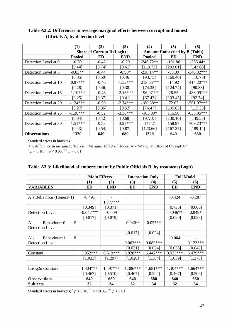
47
Table A3.2: Differences in average marginal effects between corrupt and honest
Officials A, by detection level
(1) (2) (3) (4) (5) (6)
Share of Corrupt B (Logit) Amount Embezzled by B (Tobit)
Pooled ED END Pooled ED END
Detection Level at 0 -0.70 -0.42 -0.29 -246.72** -101.86 -266.44*
[0.44] [0.74] [0.61] [119.72] [203.01] [143.68]
Detection Level at 5 -0.83** -0.44 -0.90* -230.14** -58.39 -340.32***
[0.35] [0.59] [0.46] [93.75] [160.40] [110.78]
Detection Level at 10 -0.97*** -0.46 -1.52*** -213.55*** -14.92 -414.20***
[0.28] [0.46] [0.38] [74.35] [124.74] [90.88]
Detection Level at 15 -1.10*** -0.48 -2.13*** -196.97*** 28.55 -488.09***
[0.25] [0.37] [0.41] [67.43] [103.45] [92.74]
Detection Level at 20 -1.24*** -0.50 -2.74*** -180.38** 72.02 -561.97***
[0.27] [0.35] [0.52] [76.47] [105.63] [115.33]
Detection Level at 25 -1.38*** -0.52 -3.36*** -163.80* 115.50 -635.85***
[0.34] [0.42] [0.68] [97.10] [130.10] [149.53]
Detection Level at 30 -1.51*** -0.53 -3.97*** -147.21 158.97 -709.73***
[0.43] [0.54] [0.87] [123.66] [167.35] [189.14]
Observations 1320 640 680 1320 640 680
Standard errors in brackets.
The difference in marginal effects is: “Marginal Effect of Honest A”- “Marginal Effect of Corrupt A” * p < 0.10, ** p < 0.05, *** p < 0.01
Table A3.3: Likelihood of embezzlement by Public Officials B, by treatment (Logit)
Main Effects Interaction Only Full Model
(1) (2) (3) (4) (5) (6)
VARIABLES ED END ED END ED END
A’s Behaviour (Honest=1) -0.491 -
1.777***
-0.424 -0.287
[0.349] [0.371] [0.735] [0.606]
Detection Level -0.047*** -0.009 -0.046** 0.049*
[0.017] [0.019] [0.020] [0.028]
A’s Behaviour=0 #
Detection Level
-0.040** 0.057**
[0.017] [0.024]
A’s Behaviour=1 #
Detection Level
-
0.062***
-
0.082***
-0.004 -
0.123***
[0.021] [0.024] [0.035] [0.042]
Constant 3.952*** 6.619*** 3.828*** 6.442*** 3.933*** 6.479***
[1.023] [1.297] [1.020] [1.384] [1.039] [1.378]
Lnsig2u Constant 1.304*** 1.497*** 1.306*** 1.681*** 1.304*** 1.664***
[0.467] [0.510] [0.467] [0.504] [0.467] [0.506]
Observations 640 680 640 680 640 680
Subjects 32 34 32 34 32 34
Standard errors in brackets; * p < 0.10, ** p < 0.05, *** p < 0.01

48
Table A3.4: Amount embezzled by Public Officials B – pooled data (Tobit)
Detection Levels – Continuous
(1) (2) (3)
VARIABLES Main
Effects
Interaction
Only
Full Model
(1)
Full Model
(2)
END -76.722 -88.131 -77.258 -236.376
[425.678] [426.658] [425.585] [433.890]
A’s Behaviour (Honest=1) -198.147*** -246.720** -94.841
[67.400] [119.720] [187.752]
Detection Level -10.756*** -11.554*** -19.280***
[3.047] [3.454] [5.028]
A’s Behaviour=0 # Detection Level -8.666***
[3.157]
A’s Behaviour=1 # Detection Level -16.871*** 3.317 8.358
[4.267] [6.754] [9.534]
END # A’s Behaviour=1 -184.151
[243.445]
END # Detection Level 18.806***
[6.947]
END # A’s Behaviour=1
#Detection Level
-23.602*
[13.875]
Constant [315.532] [316.228] [316.454] [319.504]
-76.722 -88.131 -77.258 -236.376
Lnsig2_u Constant 731.116*** 732.936*** 730.944*** 725.257***
[71.634] [71.795] [71.622] [71.045]
Lnsig2_e Constant 947.629*** 948.885*** 947.543*** 938.694***
[26.335] [26.374] [26.332] [26.073]
Observations 1320 1320 1320 1320
Subjects 66 66 66 66
Standard errors in brackets;* p < 0.10, ** p < 0.05, *** p < 0.01
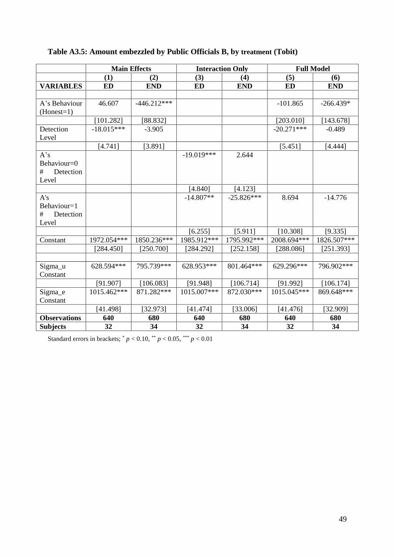
49
Table A3.5: Amount embezzled by Public Officials B, by treatment (Tobit)
Main Effects Interaction Only Full Model
(1) (2) (3) (4) (5) (6)
VARIABLES ED END ED END ED END
A’s Behaviour
(Honest=1)
46.607 -446.212*** -101.865 -266.439*
[101.282] [88.832] [203.010] [143.678]
Detection
Level
-18.015*** -3.905 -20.271*** -0.489
[4.741] [3.891] [5.451] [4.444]
A’s
Behaviour=0
# Detection
Level
-19.019*** 2.644
[4.840] [4.123]
A's
Behaviour=1
# Detection
Level
-14.807** -25.826*** 8.694 -14.776
[6.255] [5.911] [10.308] [9.335]
Constant 1972.054*** 1850.236*** 1985.912*** 1795.992*** 2008.694*** 1826.507***
[284.450] [250.700] [284.292] [252.158] [288.086] [251.393]
Sigma_u
Constant
628.594*** 795.739*** 628.953*** 801.464*** 629.296*** 796.902***
[91.907] [106.083] [91.948] [106.714] [91.992] [106.174]
Sigma_e
Constant
1015.462*** 871.282*** 1015.007*** 872.030*** 1015.045*** 869.648***
[41.498] [32.973] [41.474] [33.006] [41.476] [32.909]
Observations 640 680 640 680 640 680
Subjects 32 34 32 34 32 34
Standard errors in brackets; * p < 0.10, ** p < 0.05, *** p < 0.01

50
Appendix 4
Table A4.1: Probability of Detection Chosen by Public Officials A
Treatment Type Mean detection probability
(per cent)
Standard deviation
ED
Overall 17.21 7.33
Honest 16.51 7.99
Corrupt 17.34 6.68
END
Overall 10.52 6.36
Honest 12.58 7.08
Corrupt 11.41 7.20
Appendix 5: Regression Analysis with Detection Levels as Dummies
In the table below, we estimate the following equations:
𝑦𝑖𝑡 = 𝛼 + 𝛽𝐸𝑁𝐷 + 𝜌𝐻𝑜𝑛𝑒𝑠𝑡_𝐴𝑖𝑡 + 𝛿𝐷𝑢𝑚𝑚𝑦_𝐷𝑒𝑡𝑒𝑐𝑡𝑖𝑜𝑛𝑖𝑡 + 𝜇𝑖 + 휀𝑖𝑡 (1)
𝑦𝑖𝑡 = 𝛼 + 𝛽𝐸𝑁𝐷 + 𝛾𝐷𝑢𝑚𝑚𝑦_(𝐻𝑜𝑛𝑒𝑠𝑡_𝐴𝑖𝑡 × 𝐷𝑒𝑡𝑒𝑐𝑡𝑖𝑜𝑛𝑖𝑡) + 𝜇𝑖 + 휀𝑖𝑡 (2)
𝑦𝑖𝑡 is the dependent variable. It is either a dummy variable which equals 1 when Official B
embezzles (0 otherwise); or the amount, between 0 and 2,280ECU, embezzled by Official B
(see Section 4.2). The variable 𝐸𝑁𝐷 is a dummy variable which equals 1 for the END treatment
and 0 otherwise. 𝐻𝑜𝑛𝑒𝑠𝑡_𝐴𝑖𝑡 is a dummy variable which equals 1 when Official A is honest
and 0 otherwise. 𝐷𝑒𝑡𝑒𝑐𝑡𝑖𝑜𝑛 is the level of detection chosen by Official A. It is treated as a
dummy is created for each level of detection in Equations 1-2. 𝐻𝑜𝑛𝑒𝑠𝑡_𝐴𝑖𝑡 × 𝐷𝑒𝑡𝑒𝑐𝑡𝑖𝑜𝑛𝑖𝑡 is
an interaction of Public Official A’s behaviour with the level of detection that he/she chooses.
The constant term, individual effect term, and the error term are respectively 𝛼, 𝜇𝑖 and 휀𝑖𝑡. The
subscript 𝑖 is for individual subjects and 𝑡 denotes the round. We use a random-effects Logit
model to analyse Public Official B’s decision to embezzle or not; and a random-effects two-
sided Tobit model for the amount embezzled by Public Official B.
Column 1 of Table 5.1, in which we employ dummies for each detection level (Equation
1), we find that several levels of detection have significant and negative effects on Public
Official B’s likelihood to embezzle. In particular the 20 per cent and 30 per cent levels are
51
statistically significant at the 5 per cent and 1 per cent levels respectively. In column 2
(corresponding to Equation 2), we employ dummies for each detection level and include only
the interaction terms. Thus we take a cell-means model approach in which the baseline cell is
a corrupt Public Official A choosing a zero level of detection and all other cells are compared
to this baseline. All levels of detection (except level 0) have a statistically significant and
negative effect on Public Official B’s likelihood to be corrupt when chosen by an honest Public
Official A. In contrast, the coefficients for detection levels chosen by a corrupt Public Official
A are all insignificant. A joint equality test of the coefficients for all levels of detection yields
significant results (p-value = 0.000, chi2) suggesting that Public Official B is more likely to be
corrupt when detection is chosen by a corrupt Public Official A than when chosen by an honest
Public Official A. Once again this is evidence of a legitimacy effect.
Relative to the amount embezzled, column 3 (corresponding to Equation 1) employs a
dummy for each detection level and shows that there is a meaningful deterrence effect at all
levels of detection. This result supports the conclusion that detection is effective in curbing the
amount embezzled. Column 4 of Table 5.1 uses dummies for each detection level (Equation 2)
and finds that all levels of detection have a significant negative effect on the amount embezzled
by Public Official B when Public Official A is honest. Most levels are also significant whether
Public Official A acts corruptly or honestly, using a corrupt official choosing 0 detection level
as a baseline (Equation 5). Considering the coefficient for corrupt and honest Officials A, a
joint equality test of the coefficients for each level of detection rejects the null hypothesis of
joint equality (p-value = 0.0314, chi2). In essence, despite the presence of deterrence for both
types, Public Official B is likely to embezzle more funds when Public Official A (the policy
maker) is corrupt than when he/she is honest. This result implies that legitimacy can play a
significant role in the fight against embezzlement.

52
Table A5.1: Detection levels – dummy
Likelihood of Embezzlement
(Logit)
Amount Embezzled (Tobit)
(1) (2) (3) (4)
VARIABLES Main Effects Interaction
Only
Main
Effects
Interaction
Only
END 0.599 0.615 22.636 44.585
[0.698] [0.713] [192.130] [192.371]
A’s Behaviour (Honest=1) -1.191*** -191.624***
[0.249] [67.339]
Detection Level
A’s Behaviour=0 # Detection
Level
A’s Behaviour=1 # Detection
Level
Detection Level=5 -0.512 -304.588***
[0.470] [100.041]
Detection Level=10 -0.698 -363.048***
[0.477] [109.614]
Detection Level=15 -0.765* -397.836***
[0.451] [110.310]
Detection Level=20 -0.983** -404.543***
[0.443] [100.895]
Detection Level=25 -0.438 -255.449**
[0.474] [114.025]
Detection Level=30 -1.273*** -428.595***
[0.435] [103.949]
A’s Behaviour=0 # Detection
Level=5
-0.393 -257.555**
[0.622] [113.599]
A’s Behaviour=0 # Detection
Level=10
-0.690 -263.998**
[0.603] [126.544]
A’s Behaviour=0 # Detection
Level=15
-0.461 -247.005*
[0.614] [131.626]
A’s Behaviour=0 # Detection
Level=20
-0.815 -383.438***
[0.549] [111.624]
A’s Behaviour=0 # Detection
Level=25
-0.230 -275.637**
[0.631] [132.903]
A’s Behaviour=0 # Detection
Level=30
-0.900* -386.808***
[0.542] [118.230]
A’s Behaviour=1 # Detection
Level=0
-0.763 1.250
[0.667] [172.500]
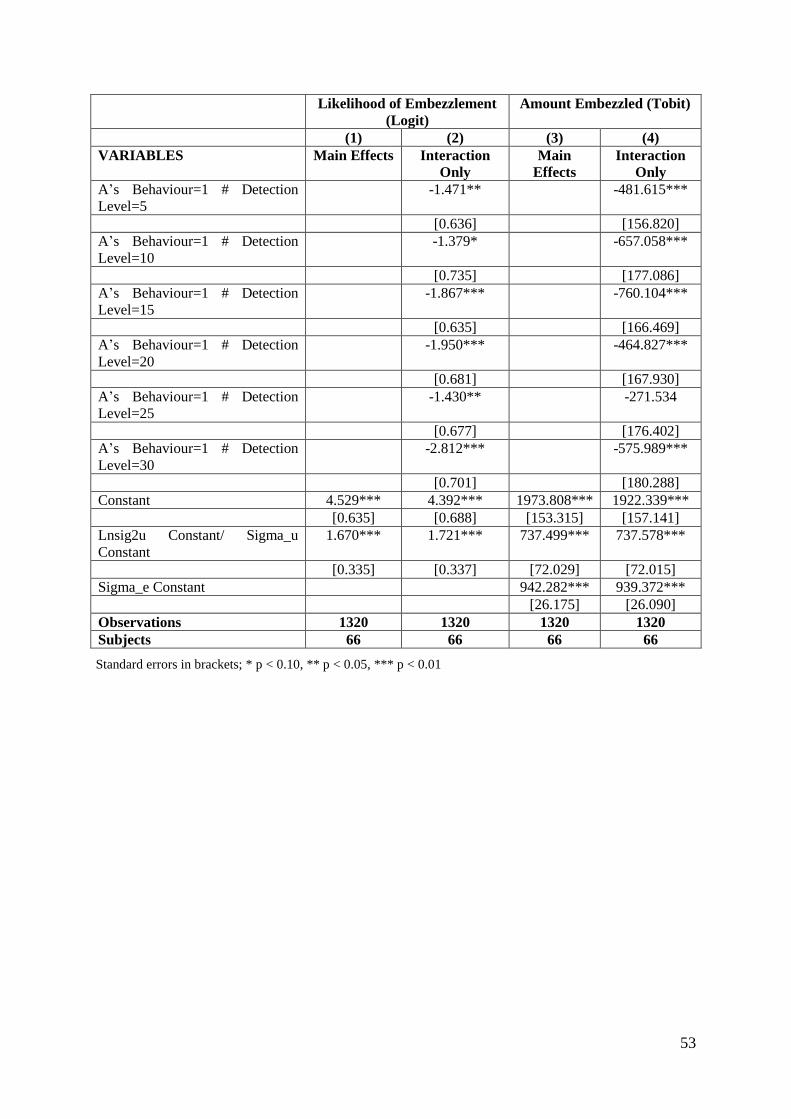
53
Likelihood of Embezzlement
(Logit)
Amount Embezzled (Tobit)
(1) (2) (3) (4)
VARIABLES Main Effects Interaction
Only
Main
Effects
Interaction
Only
A’s Behaviour=1 # Detection
Level=5
-1.471** -481.615***
[0.636] [156.820]
A’s Behaviour=1 # Detection
Level=10
-1.379* -657.058***
[0.735] [177.086]
A’s Behaviour=1 # Detection
Level=15
-1.867*** -760.104***
[0.635] [166.469]
A’s Behaviour=1 # Detection
Level=20
-1.950*** -464.827***
[0.681] [167.930]
A’s Behaviour=1 # Detection
Level=25
-1.430** -271.534
[0.677] [176.402]
A’s Behaviour=1 # Detection
Level=30
-2.812*** -575.989***
[0.701] [180.288]
Constant 4.529*** 4.392*** 1973.808*** 1922.339***
[0.635] [0.688] [153.315] [157.141]
Lnsig2u Constant/ Sigma_u
Constant
1.670*** 1.721*** 737.499*** 737.578***
[0.335] [0.337] [72.029] [72.015]
Sigma_e Constant 942.282*** 939.372***
[26.175] [26.090]
Observations 1320 1320 1320 1320
Subjects 66 66 66 66
Standard errors in brackets; * p < 0.10, ** p < 0.05, *** p < 0.01