determining the fate and transport of the acrylamide · pdf filedetermining the fate and...
TRANSCRIPT
DETERMINING THE FATE AND TRANSPORT OF THE ACRYLAMIDE
MONOMER (AMD) IN SOIL AND GROUNDWATER SYSTEMS
by
Todd James Arrowood
Bachelor of Science in Geology University of Nevada, Las Vegas
2005
A thesis submitted in partial fulfillment
of the requirements for the
Master of Science Degree in Geoscience Department of Geoscience
College of Sciences
Graduate College University of Nevada, Las Vegas
May 2008

ii
(Approval Page)

iii
ABSTRACT
Determining the Fate and Transport of the Acrylamide Monomer (AMD) in Soil
and Groundwater Systems
by
Todd James Arrowood
Dr. Zhongbo Yu, Examination Committee Chair Associate Professor of Hydrogeology
University of Nevada, Las Vegas
Dr. Michael H. Young, Examination Committee Co-Chair Associate Research Professor, Division of Hydrologic Sciences
Desert Research Institute (DRI)
Acrylamide (AMD) is a known animal and suspected human carcinogen and is used
to produce polyacrylamide (PAM), which has been proposed as a technology for seepage
control in unlined water delivery canals. Previous studies have not quantified the fate and
transport of AMD in soil and groundwater systems. In this study, batch experiments and
soil column tests (with and without microbial degradation) were conducted on three
materials (control sand, gravelly sand and loam soil) to determine the Kd, retardation
factor, the form of the sorption isotherm, and determine microbial degradation rates. Soil
core tests from samples collected in canals were also conducted to simulate field-scale
transport. A numerical model (HYDRUS-2D) was used to simulate a canal environment
using the fate and transport parameters of AMD obtained in the laboratory. Results
indicate a Freundlich-type sorption isotherm for AMD in the loam soil and a linear

iv
isotherm for the sandy material. Sorption values were 0-2.4% in all tests. Results for the
soil column tests show that AMD is conservative in all three types of material tested. The
bacteria column tests indicated that AMD was quickly degraded (half lives were less than
3 hours), though half lives for the canal column tests were longer (~31 hours). Numerical
modeling shows that AMD would not be detectable 25 meters from the canal, as long as
initial AMD concentration is less than 6.65 ppb. Using PAM at concentrations of less
than 13 ppm would inhibit detectable contamination of canal water.

v
TABLE OF CONTENTS ABSTRACT……............................................................................................................... iii TABLE OF CONTENTS.....................................................................................................v LIST OF FIGURES .......................................................................................................... vii LIST OF TABLES........................................................................................................... viii ACKNOWLEDGEMENTS............................................................................................... ix CHAPTER 1 INTRODUCTION ........................................................................................1 CHAPTER 2 LITERATURE REVIEW .............................................................................8
2.1 Previous agricultural PAM usage ............................................................................. 8 2.2 Possible PAM breakdown to AMD ........................................................................ 10 2.3 PAM and AMD transport........................................................................................ 13 2.4 AMD microbial breakdown .................................................................................... 16
CHAPTER 3 MATERIALS, METHODOLOGY, AND DATA DESCRIPTION...........20
3.1 Description of soil material..................................................................................... 20 3.2 HPLC chemical analysis ......................................................................................... 22 3.3 Experiment 1: AMD sorption batch tests................................................................ 23
3.3.1 Experimental setup........................................................................................... 26 3.3.2 Determining sorption significance................................................................... 27 3.3.3 Determining sorption isotherms and retardation factors.................................. 28
3.4 Experiment 2: AMD degradation flask study ......................................................... 29 3.4.1 Experimental design......................................................................................... 30 3.4.2 Determining flask sterility ............................................................................... 30 3.4.3 Determining half life, degradation rate, and degradation percentage.............. 31
3.5 Experiment 3: column tests..................................................................................... 31 3.5.1 Experimental design......................................................................................... 32 3.5.2 Experimental setup........................................................................................... 32
3.5.2.1 Test solution for column tests ................................................................... 35 3.5.2.2 Soil column preparation............................................................................ 36 3.5.2.3 Pulse and step inputs for breakthrough curves ......................................... 39
3.5.3 Determining AMD/bromide breakthrough curves........................................... 40 3.5.4 Determining AMD sorption............................................................................. 42
3.6 Repacked bacteria inoculated column tests ............................................................ 42 3.6.1 Experimental setup........................................................................................... 43
vi
3.6.1.1 Test solution for column tests ................................................................... 44 3.6.1.2 Isolation and characterization of column test bacterium .......................... 44
3.6.2 Determining AMD degradation rate, percentage, and half-life ....................... 45 3.7 Experiment 5: canal soil core column tests............................................................. 45
3.7.1 Experimental design/setup ............................................................................... 45 3.7.2 Determining column degradation rate, half-life and percentage ..................... 46
3.8 Predictive numerical modeling with HYDRUS-2D ............................................... 46 3.9 Statistical analysis................................................................................................... 50
3.9.1 Analysis of variance......................................................................................... 50 3.9.2 Multiple comparison ........................................................................................ 52 3.9.3 ANCOVA statistical analysis .......................................................................... 52
CHAPTER 4 DATA ANALYSIS ....................................................................................55
4.1 Soil physical properties........................................................................................... 55 4.1.1 Particle size distribution................................................................................... 55 4.1.2 Surface area analysis........................................................................................ 55 4.1.3 Total organic content (TOC) analysis.............................................................. 57
4.2 Experiment 1: AMD sorption batch tests................................................................ 58 4.2.1 Sorptive characteristics of AMD ..................................................................... 58 4.2.2 Sorption isotherms ........................................................................................... 61
4.3 Experiment 2: AMD degradation flask study ......................................................... 64 4.3.1 Flask degradation rates .................................................................................... 64 4.3.2 Flask sterility analysis...................................................................................... 66
4.4 Experiment 3: repacked column tests ..................................................................... 66 4.4.1 Analysis of breakthrough curves ..................................................................... 66 4.4.2 Column sorption isotherms .............................................................................. 70 4.4.2 Comparing batch and column sorption isotherms and retardation values ....... 72
4.5 Experiment 4: bacteria inoculated repacked column tests ...................................... 73 4.5.1 Breakthrough curve analysis............................................................................ 73 4.5.2 Bacteria column degradation rates and half lives ............................................ 73 4.5.3 Bacterial and competing nitrogen analysis ...................................................... 80
4.6 Experiment 5: canal soil core column tests............................................................. 81 4.6.1 Breakthrough curve analysis............................................................................ 81 4.6.2 Canal column degradation rates....................................................................... 81 4.6.3 Bacterial analysis ............................................................................................. 84
4.7 Results for the predictive numerical modeling with HYDRUS-2D ....................... 84 CHAPTER 5 CONCLUSIONS AND RECOMMENDATIONS.....................................94 APPENDIX. GRPAHS OF COLUMN EXPERIMENTS.................................................98 REFERENCES… ............................................................................................................114 VITA………….. ..............................................................................................................123

vii
LIST OF FIGURES
Figure 1.1: Macromolecular and molecular structure of non-crosslinked polyacrylamide (Modified from Holliman et al., 2005) ...........................5 Figure 2.1: AMD production and degradation (Labahn, 2007).................................19 Figure 3.1: Determination of MDL by the Hubaux and Vos (1970) method............24 Figure 3.2: Setup for the repacked column experiment ............................................33 Figure 3.3: Soil column used for experiments...........................................................37 Figure 3.4: Pictures of (A) soil column funnel apparatus and (B) packing a column.....................................................................................................38 Figure 3.5A: Case study for PAM lined canal in the HYDRUS-2D program .............49 Figure 3.5B: Pressure gradients for the canal with 5-meter water table depth ............49 Figure 4.1: Concentrations of AMD sorbed onto non-autoclaved soil .....................62 Figure 4.2: Concentrations of AMD sorbed onto autoclaved soil.............................62 Figure 4.3: Graph of flask data and degradation rates (symbols are observed data, lines are fitted degradation rates) ...................................................65 Figure 4.4: Graphs of (A) bacterial column tests with C33 sand and experienced bacteria without competing nitrogen, and (B) with competing nitrogen ...................................................................................................74 Figure 4.4: Graphs of (C) bacterial column tests with C33 sand and naïve bacteria without competing nitrogen, and (D) with competing nitrogen ...................................................................................................75 Figure 4.4: Graphs of (E) bacterial column tests with loam soil and experienced bacteria without competing nitrogen, and (F) with competing nitrogen ...................................................................................................76 Figure 4.4: Graphs of (G) bacterial column tests with loam soil and experienced bacteria without competing nitrogen, and (H) with competing nitrogen ...................................................................................................77 Figure 4.4: Graphs of (I) bacterial column tests with C33 sand, no bacteria, without competing nitrogen, and (J) loam soil, no bacteria, without competing nitrogen .................................................................................78 Figure 4.5: Graphs of (A) bacterial soil core column tests Site 1 – Column 1, and (B) Site 1 – Column 2 ......................................................................82 Figure 4.5: Graphs of (C) bacterial soil core column tests Site 2 – Column 1, and (D) Site 2 – Column 2 ......................................................................83 Figure 4.6: Graphs of a HYDRUS model run (C33 sand, partial seal, PAM conductivity level of 10 lb/ca, at water table depth of 0 meters) (A) with out sorption or bacterial degradation and, (B) with the added affects of sorption and bacterial degradation ..........................................89

viii
LIST OF TABLES
Table 1.1: Chemical and physical properties of acrylamide ......................................4 Table 3.1: Critical level and minimum detection limit for all experiments .............24 Table 3.2: Outline of experimental design for batch experiments ...........................25 Table 3.3: General setup for bromide/AMD column tests.......................................33 Table 3.4: Outline of HYDRUS test design.............................................................49 Table 3.5: Observation node properties ...................................................................51 Table 4.1: Particle size distributions of fine-earth fraction (< 2 mm) for three soil materials used in the research. .........................................................56 Table 4.2: Particle size analysis for C33 sand and loam soil autoclaved samples...56 Table 4.3: Change in grain size for C33 sand and loam from autoclaving cycles...57 Table 4.4: Surface area analysis...............................................................................57 Table 4.5: Results from the un-autoclaved tests for all mixing times......................59 Table 4.6: Results from the autoclaved tests for all mixing times ...........................60 Table 4.7: Correlation coefficients for isotherms ....................................................63 Table 4.8: Estimated retardation values ...................................................................63 Table 4.9: Estimated flask degradation values.........................................................65 Table 4.10: Recovery and experimental conditions for soil column experiments .....68 Table 4.11: Estimated transport parameters for the soil column test.........................69 Table 4.12: ANOVA and ANCOVA statistics for AMD parameter comparisons ....71 Table 4.13: Multiple comparison statistics for parameter comparisons ....................71 Table 4.14: Correlation coefficients for isotherms ....................................................73 Table 4.15: Degradation parameters for bacterial column tests.................................79 Table 4.16: Results of ANOVA analyses for parameter comparisons.......................80 Table 4.17: Degradation parameters for bacterial column tests.................................84 Table 4.18: Model observation node data for the no sorption, no bacterial degradation models .................................................................................86 Table 4.19: Model observation node data incorporating sorption but ignoring microbial degradation. ............................................................................87 Table 4.20: Model observation node data, including processes of sorption and bacterial degradation models ..................................................................88 Table 4.21: Arrival times of peak concentrations with no treatment and a partial seal for #70 mesh and C33 sand .............................................................91 Table 4.22: Arrival times of peak concentration with no treatment and a partial seal for #70 mesh and C33 sand, including microbial degradation of AMD .......................................................................................................91

ix
ACKNOWLEDGEMENTS
I would like to thank: The US Bureau of Reclamation for providing the funding to conduct PAM and
AMD research under cooperative agreement #04-FC-81-1064. Dr. Michael H. Young for giving me the opportunity to work on this project,
providing me with a graduate research assistantship and for so much advice and support in helping me finish this project.
Dr. Zhongbo Yu and all his help along the way in my undergraduate and graduate
work with feedback reviews, education, and all the help with computer modeling. My committee members Dr. Dave Kreamer and Dr. Thomas Piechota for the
feedback they provided and taking the time and effort to review this document. PAM peer review committee for constructive feedback
Dr. Duane Moser for helping me understand the small, vast world of
microbiology and bacteria and all the feedback. Ernesto Moran for helping me in the lab and giving me so much feedback, help,
equipment, training, and memories. Stephanie Labahn for all the help and assistance with experiments, setup, and the
knowledge of microbiology. John Goreham and Dr. Darren Meadows for teaching me so much in the lab and
keeping my spirits up. Jennifer Barth, Karen Levy, Christina Jacovides, Journet Wallace, for their help.
Jim Woodrow and Dr. Glenn Miller for their help in getting me familiar with
HPLC and their input and feedback for this project. All UNLV Geoscience Faculty and Staff and all the wonderful students and
researchers at UNLV and DRI who were such a big part of my life these last few years.
My parents for all their love and support

1
CHAPTER 1
INTRODUCTION
The decreasing amounts of fresh water supply and the need to conserve water in arid
regions of the western United States are growing concerns. Low-cost and effective
methods to minimize loss of water in unlined water delivery canals (the canals that
convey water from reservoirs or rivers to end users) would have a major positive effect
on conservation efforts. Alternative methods to reduce water loss in water delivery canals
can be expensive, such as lining with concrete or plastic. The use of polyacrylamide
(PAM) as a canal sealant may conserve water, but the possible health issues with the
acrylamide monomer (AMD) found in the PAM molecule must be addressed.
To help conserve water, the U.S. Bureau of Reclamation (USBR) is evaluating the
use of PAM to seal unlined water delivery canals. However, very little is known about
the fate and transport characteristics of AMD in the soil/groundwater environment; thus,
research is needed to determine transport parameters, to help understand AMD transport
through soil and the factors that affect its movement. With an increased understanding of
AMD fate and transport through soil and groundwater systems, a more thorough
evaluation of this use of PAM can be made.
PAM is an ultra-high molecular weight polymer that has been used in many fields for
up to 50 years. PAM is used for wastewater treatment, paper and pulp industries,
consumer goods, agricultural uses, mineral processing, oil drilling projects, and as a

2
water well and sewer pipe line sealant (EPA, 1994a; European Union Risk Assessment,
2002). In agriculture, PAM is currently used to stabilize soil structure in agricultural
irrigation furrow, causing more uniform infiltration and limiting soil erosion (Sojka and
Lentz, 1994; Spofford and Pfeiffer, 1996). The proposed new use of PAM as a canal
sealant is based on research showing that higher concentrations of PAM can decrease
infiltration in soil (Malik and Letey, 1992; Nadler et al., 1994; Letey, 1996; Lentz, 2003;
Ajwa and Trout, 2006).
PAM is formed through a polymerization process which takes millions of AMD
molecules and chains them together to make a single molecule of PAM. Many forms of
PAM exist. Linear anionic PAM is generally used in agriculture. This form is made with
acrylic acid so it is anionic or has a slight positive charge. In the production of PAM,
0.025 % to 0.05 % of residual AMD is left in the PAM molecule (Sojka et al., 1998a).
Therefore, if the PAM is added to the canal water at concentrations of 1 ppm, then the
AMD concentration released from the hydrated PAM molecule should not exceed 0.5
ppb, or the current EPA maximum concentration limit. Research has shown that PAM
itself has a low level of human toxicity (Lentz et al., 2002; Smith et al., 1996).
The AMD monomer used in the production of PAM is known to be a human
neurotoxin and is believed to be a human carcinogen, causing damage to cells on the
DNA level. AMD is already a known animal carcinogen and neurotoxin (EPA, 1994a and
b). EPA reported that exposures to humans have been associated with polyneuropathy
with motor and sensory impairment marked by numbness, paresthesias, ataxia, tremor,
dysarthria, and mid-brain lesions. Ingestion of contaminated drinking water has caused
drowsiness, disturbances of balance, confusion, memory loss, and hallucinations (EPA,

3
1994b). The current standard for AMD in water is 0.5 ppb and 0.25 ppb in the United
States and Europe, respectively (EPA, 1994b; European Union Risk Assessment, 2002).
Chemical and physical properties of acrylamide are summarized below in Table 1.1
(European Union Risk Assessment, 2002). Acrylamide is solid at room temperature,
highly soluble in water, has a low potential to partition to organic matter, and has a low
volatilization potential in water.
When PAM hydrates, it expands and forms a random coiled structure (Figure 1.1) and
then moves with the water, attaches to suspended particles and sinks to the bottom of
channel. It then adheres to the soil on the bottom of the canal by forces of electrostatic,
hydrogen and chemical bonding (Lentz et al., 2002). The residual AMD in the PAM
molecule can be released from the PAM molecule in different areas of the canal. First,
the AMD molecule may be released when PAM is initially saturated; second, AMD may
be released after PAM has settled to the canal surface and is sealing the canal; and third
AMD may be released if PAM is transported into the subsurface of the canal, though
research has shown that PAM transport beyond a meter depth into soil is very unlikely
(Malik and Letey, 1991; Nadler et al., 1992; Nadler et al., 1994). The rate of release of
AMD is thus an important consideration when estimating the downstream concentrations.
The nature of this research is to examine the fate and transport of the AMD monomer
from the application of non-crosslinked, anionic, straight chain PAM, when used as a
canal sealant. This project is part of a collaborative research effort between several
groups: The United States Bureau of Reclamation (USBR), the Desert Research Institute
(DRI), the University of Nevada, Las Vegas (UNLV), and the University of Nevada,
Reno (UNR). Field tests in Grand Junction, Colorado (and elsewhere) on PAM as well as

4
Table 1.1: Chemical and physical properties of acrylamide
International Union of Pure and
Applied Chemistry (IUPAC) Name:
Acrylamide
Structural formula: CH2=CH-CONH2
Molecular formula: C3H5NO
Chemical Abstracts Service (CAS) No.: 79-06-1
Molecular weight (MW): 71.09
Synonyms: acrylic acid amide, 2-propenamide, ethylene carboxamide, propenoic acid amide, vinyl amide
Physical state: White crystalline solid at 25 oC Solubility: 2040 gm/L (25 oC)
2155 gm/L (30 oC) Melting point: 84-84.5 °C Vapor pressure: 0.9 Pa at 25 °C for solid AMD
4.4 Pa at 40 °C for solid AMD Density 1.127 gm/cm3 at 30 °C
N-octanol-water partition coefficient (KOW):
-1.0
Flash Point n/a-however can polymerize exothermically above melting point
Explosivity As above

5
Figure 1.1: Macromolecular and molecular structure of non-crosslinked polyacrylamide (Modified from Holliman et al., 2005)
other lab experiments are concurrently being conducted by DRI and UNR. Information
from these collaborators provided basic scientific data for testing predictive models. In
addition to the research conducted in this thesis, the overall PAM program will provide a
better understanding of how and at what rate PAM releases AMD, potential microbial
breakdown rates of PAM, and the potential for PAM and AMD bioaccumulation. Soil
column testing and computer modeling of AMD transport in soil and groundwater
systems, as will be discussed below, can provide enhanced insight into the conditions that
are being tested in field-scale canals. The research findings here will supplement the

6
research being done at sites in Colorado, and other research being done by researcher at
DRI and UNR. With this combined research effort, a better understanding of the fate and
transport of AMD introduced into the system by means of application of PAM in water
delivery canals and the environmental impact of this application of PAM will be
determined.
The overall goal of this study is to determine the fate and transport of AMD in
soil/groundwater systems. The objectives of this research are to: 1) determine the Kd
value of AMD, create a sorption isotherm for AMD, and determine if AMD sorption is
kinetic or instantaneous; 2) determine the breakthrough curve for the AMD transport
experiments; 3) determine AMD transport behavior in sterile soil; 4) examine microbial
breakdown of AMD in soil systems; and, 5) simulate the fate and transport of AMD
through groundwater.
The hypotheses for this study are that 1) the Kd value for AMD will be low, but a
small amount of adsorption will occur, AMD sorption will be instantaneous, leading the
AMD molecule to be a mobile solute; 2) AMD will be degrade by bacteria, which will
lower AMD concentrations with time; and 3) degradation pathways will influence level
of potential AMD contamination in a shallow ground-water system. To address the
hypotheses, as series of laboratory and numerical experiments were conducted, including,
1) batch and (abiotic) column experiments for measuring sorption levels and kinetics; 2)
bacteria-inoculated column and natural (undisturbed) canal column tests for measuring
rates and amounts of microbial degradation of AMD with time; and 3) numerical
simulations to examine sensitivity of AMD concentration to combinations of degradation

7
pathways and field conditions. The methods used to carry out these objectives are
explained in the methods section below.
This thesis is divided into chapters that present different aspects of the study. Chapter
2 is a literature review that discusses past work related to PAM agricultural use, PAM
degradation, AMD transport, and AMD microbial degradation. Chapter 3 describes in
detail the methods and techniques used for the experiments in this study. Chapter 4
provides the results from the testing, and Chapter 5 presents final conclusions and future
recommendations.
8
CHAPTER 2
LITERATURE REVIEW
This study focused on the fate and transport of AMD when released from PAM, when
used as a sealant for water delivery canals. This section includes relevant literature in this
area, and it includes a review of possible release mechanisms of AMD.
2.1 Previous agricultural PAM usage
Polyacrylonitrile, the predecessor to PAM, was used in the early 1950’s to decrease
furrow erosion and increase aggregate stability. A study of its resulting increase in crop
yield was published by Bear (1952). Due to its high cost, PAM was later formulated.
Many studies have been conducted on PAM’s ability to stabilize soil structure (Helalia
and Letey, 1988; Lentz et al., 1992), its uses for erosion control (Lentz et al., 1992; Lentz
and Sojka, 1994; Sojka et al., 1998b) and it use to increase infiltration rates (Sojka et al.
(1998c). Most of these studies used field tests on irrigation furrows using anionic PAM.
These studies also showed that about 10 ppm PAM would effectively decrease erosion at
a reasonable cost, and that 5 to 10 ppm would increase infiltration rates by helping
stabilize existing soil structure.
Work by Letey (1996) showed that concentrations above 10 ppm PAM decreased
infiltration due to increases in viscosity. Lentz (2003), however, suggested that a decrease

9
in infiltration between 10-50% can be achieved by surface sealing. The study showed that
PAM created a seal at the soil/water interface, decreasing the ability of water to infiltrate.
The concentration of a mass of PAM in a volume of water (i.e., mg/L or ppm) does
not directly correlate to how PAM is applied in the field. Because PAM is designed to
treat a specific area of the canal, it is expressed in units of mass applied per area of
coverage. The most common unit used in the field is pounds per canal acre (lbs/ca).
These units imply that a solution concentration of 10 ppm would cover the same area as a
solution containing ten times the water, yielding a concentration of 1 ppm; therefore, the
amount of PAM applied to an area is independent of the volume of water or the solution
concentration. Moran (2007) showed that a PAM application rate of 10 lbs/ca can
decrease hydraulic conductivity of sandy soil by more than 90%, depending on the
suspended sediment concentration. The concentration levels of PAM that could result
from canal treatment can be adjusted by using more or less water; however managing
PAM concentrations in this way could influence the velocity in the canal and affect the
area of coverage depending on the settling rate of PAM. If the concentration of PAM in
the water can be kept below 1 ppm (the EPA drinking water standard), and if the residual
AMD concentration in the PAM molecule is less than 0.05%, as required by the National
Sanitary Foundation (NSF Standard 60), then the concentration of AMD will never rise
above the EPA drinking water standard of 0.5 ppb (Code of Federal Regulations [40 CFR
§141.111]), assuming all AMD released is residually held in the PAM molecule and not
created from possible PAM degradation.

10
2.2 Possible PAM breakdown to AMD
Smith et al. (1996) tested a PAM thickening agent (PATA) used to thicken mixtures
of herbicides and pesticide applications to crops, to evaluate if PATA might degrade to
AMD under artificial environmental conditions. They also tested its effects with a
glyphosate-surfactant herbicide (GH). They ran tests for differing pH levels (5, 6, 7, 8, 9)
kept at 25 ºC with various light/dark cycles at temperatures range from 4 to 37ºC, under
light conditions simulated by a florescent lamp with wavelengths at 300 - 700 nm. The
samples were measured once every week using high performance liquid chromatography
(HPLC) to determine AMD and ammonia concentrations. They found that under artificial
conditions PATA without GH did not degrade to AMD, but that AMD did degrade and
did so faster in the 24 hour light studies and in the higher temperature (37 ºC) studies.
However, when PATA was mixed with GH, the AMD levels stayed consistent or
increased regardless of temperature or light exposure, indicating that the GH either
slowed down AMD degradation or that it caused a release of AMD from the PATA.
Increases in observed ammonia concentration were thought to be caused by AMD
degradation; however, using the ammonia concentrations alone precluded statistically
differentiating the source of AMD, from either breakdown of the PAM molecule or
release of AMD. They found that differing pH levels did not have any effect on the AMD
degradation.
Smith et al. (1997) continued the work from Smith et al. (1996) by testing the same
parameters of PATA and GH in outdoor conditions. The concentrations of PATA and GH
were the same as used in the previous study. Outdoor tests were conducted with water
sampled from a creek, pond, natural spring, and two wells. Distilled water was used as a

11
control. The water and differing concentrations of PATA and GH treatments were placed
in 50mL tubes and subjected to outdoor conditions of light and temperature. Undisturbed
soil core samples of three types of soil (sand, sandy loam, and silt loam) were tested
using the highest concentration of PATA with GH solution. They washed the column
with 100 mL of the solution and collected samples every 8 hours for one week. They also
set up soil boxes with the same soils oriented at a 5° angle to test for AMD movement in
the runoff water. In all the water tests, AMD concentrations increased and then tapered
off except in the natural spring water and in one of the wells where the concentrations
increased and remained elevated. In the soil column test, AMD recovery was 97%, 73%,
and 43% for the sand, sandy loam, and silt loam, respectively. The soil box tests showed
no detectable AMD runoff from surface water. Smith et al. (1997) concluded that PATA
degrades to AMD in outdoor environments based on the increased concentrations found
in the waters tested, and that AMD is mobile in the soil system. The soil column tests
showed only that AMD was mobile in soil, but they did not quantify the Kd values or
present a breakthrough curve for AMD. Smith et al. (1997) state that PATA can contain
from 0.05- 5.00% residual AMD depending on purity, but they never state the quality of
the PATA used in their studies. Thus, the residual AMD released into the environment,
versus the possible formation of AMD from PAM breakdown, can not be determined.
Vers (1999) studied the degradation of PAM to AMD in the presence of GH and sunlight.
Vers’ objective was to support or refute the hypothesis that PAM degradation to AMD
could happen through a photolytically induced free-radical process made by Smith et al.
(1997). Vers developed a procedure to measure AMD using HPLC analysis. He used tap,
river and lake water samples and tested for the UV degradation by exposing the samples
12
to outdoor ambient conditions for six weeks. According to Vers (1999), the HPLC assay
used by Smith et al. (1996 and 1997) cannot separate acrylic acid and AMD or separate
GH and AMD. The elution curves for these samples overlap, and would thus lead to a
false positive for AMD, when only acrylic acid and GH were present. According to Vers
study, no degradation pathway from PAM to AMD was detected in the presence of
sunlight or GH using an improved HPLC different method that independently quantifies
AMD, acrylic acid and GH.
Holliman et al. (2005) studied the degradation of cross-linked PAM in the field by
aging samples of slate waste with PAM for 0 (control), 18, 43, and 72 months. They then
subsampled the soil and subjected the samples to UV exposure, pH treatment,
temperature treatment, and biodegradation. They found that only exposure to
temperatures of 35°C showed an increase of AMD and acrylic acid above drinking water
standards. The concentrations of AMD recorded from Holliman’s experiments ranged
from levels below detection limits for most samples to 453 ± 42 ppb in new PAM in
35°C soil.
Woodrow and Miller (2007) examined potential UV degradation of PAM in a semi-
controlled outdoor experiment. Several sets of tests were conducted with 15 ppm PAM
added to 100 mL of DI water in 125 mL flasks. A subset of the samples contained either
humid acid or ferrous sulfate heptahydrate at 10 ppm. Another subset of samples
contained 15 ppm PAM, 40 mL of irrigation canal water, and 3 ppm ferrous iron. All
flasks were sealed with glass stoppers and placed outside on a building roof where they
received unobstructed exposure to summer sunlight from dawn to dusk. A set of duplicate
samples placed on the same roof were wrapped in aluminum foil as a control. During the

13
experiment temperature ranged from 30-40°C and UVA light intensity (320-390 nm)
reached a maximum intensity of 2.4 mW/cm2. Samples from the 100 mL DI water test
were taken every hour for the first 8 hours, then every 24 hours, and then once a week.
Samples from the 40 mL irrigation canal tests were taken every hour for the first 8 hours
and a sample was taken at 24 hours at the end of the experiment. Samples were analyzed
for PAM and AMD. Woodrow and Miller concluded that PAM degradation rates in DI
water and irrigation water were the same. The half-lives for the PAM in only water, PAM
with humic acid, and PAM with iron were 45 days, 5 days, and 3-4 hours respectively.
AMD concentrations in the solution indicated release of residual AMD only. Results
indicated that, if AMD was being released from the degradation of PAM, then the
degradation rate was not high enough to replace AMD that was degrading.
The previous research done on PAM degradation indicates that AMD may be created
in high temperature (>35°C) environments and when in contact with direct sunlight.
However, PAM rarely if ever will be subjected to these elevated temperatures or
experience prolonged exposure to direct sunlight in a canal environment.
2.3 PAM and AMD transport
Malik and Letey (1991) determined the adsorption isotherms of PAM using batch
studies with tritium-labeled PAM at different concentrations and at different charge
densities in three different soils. They defined sorption as linear, and quantified it using
the parameter Kd, which is included in:
wds CKC (1)

14
where Cs is the concentration of the chemical of interest sorbed to the soil, Kd is the linear
sorption coefficient, and Cw is the concentration of the chemical of interest in the
solution. They determined that sorption of PAM was restricted to the external aggregate
surface and that PAM sorbed better at higher charge densities. They calculated the Kd
values for PAM to be 0.163, 0.190, and 0.145 for the 2% charge density; 1.046, 1.049,
and 0.936 for the 21 % charge density; and 0.280, 0.291, and 0.327 for the 40 % charge
density in the coarse-loamy soil, fine sand, and fine loamy soil, respectively. These
results show that PAM adheres readily and strongly to soil surfaces. Presumably, this
would indicate that PAM will also sorb strongly to soils at the bottom of water delivery
canals.
Nadler et al. (1992) tested PAM desorption from soil using the same soil and PAM
types as Malik and Letey (1991). They mixed 20 mL of solution containing PAM at
concentrations of 120, 180, 240, 300, 400 ppm into 30 grams of soil for 16 hours,
centrifuged the samples at 5000 rpm for 30 minutes, and decanted the solution. They then
added 20 mL of DI water, shook the samples for an additional 16 hours, and centrifuged
and sampled the supernatant for desorbed PAM. They also dried the soil, re-wetted it and
then quantified the remobilization of PAM. They found that less than 10 percent of PAM
desorbed from the soil and that, after the soil was dried and re-wetted, almost no PAM
was released. They determined that very little PAM would desorb if soil was kept wet
and that PAM would remain on the soil even after drying, due to irreversible bond
between the polymer and soil. They concluded the mobility of PAM to be very low and
even lower after drying.

15
Nadler et al. (1994) tested the same formulation of PAM as Nadler et al. (1992) (i.e.,
2 % charge density, tritium-labeled) on two natural sandy loam and clayey loams soils in
field sites in Israel. They excavated holes 0.4 x 0.4 meters wide and 0.25 meters deep and
mixed 1, 2, and 3 grams of PAM into 4, 8, and 12 L of water, thus keeping a constant 250
ppm PAM in solution. After soaking, the original soil was replaced and left undisturbed
for 10 months. During this time, 920 mm and 720 mm of water was used to irrigate the
sandy loam and clayey loam sites, respectively. They found that the highest concentration
of PAM in the sandy loam traveled to a depth of 0.42 meters, or about 17 cm deeper than
the depth of application. No significant levels of PAM were detected below 0.45 meters
in any of the sites. This shows that PAM mobility in soils is extremely limited and will
not travel appreciably below the application area.
Research by Lande et al. (1979) shows that acrylamide is mobile in soil. Their
research was done with soil thin-layer chromatography, which uses soil slurry for
analysis. They also determined AMD half life, using liquid scintillation to analyze 14CO2
evolution, for aerobic (18-45 hours) and anaerobic (336 hours) conditions. Their work
suggests that AMD persistence is greater in soils with lower microbial activity, and is
greater in sandy soils than clay soils.
Brown et al. (1980) tested the sorption of AMD using distilled water, sea water, sea
water with sediment, estuarine water, estuarine water with sediment, river water, river
water with sediment, sewage works water, and sewage works water with sludge. They
also tested adsorption onto kaolinite and montmorillonite clays, peat, cation exchange,
anion exchange, and hydrophobic synthetic resins and neutral, acidic, and alkali activated
carbons, all using autoclaved sterilized river water. The tests with sediment used 5 gm of

16
sediment with one liter of AMD solution at concentrations of 0.5 mg/L (500 ppb) and 10
mg/L (10,000 ppb). Samples were collected at 4- 24-, and 168-hour intervals. All samples
showed no loss at 4 hours except samples treated with activated carbon, which showed a
~95% loss in the 0.5 mg/L and ~60% loss in the 10 mg/L samples. Almost all treatments
showed no additional loss at 24 hours; however, at 168 hours all of the samples showed
significant losses, most at 100% loss except sea water, DI water and sterilized river water
with no sediments, which showed little or no loss. They concluded that sorptive processes
were insignificant or undetectable but that bacterial degradation occurred in all the
samples except the sea water, DI water and sterilized river water. Unfortunately the
sampling intervals used were not sufficient to quantify any microbial degradation rates.
Also they did not state the accuracy of their HPLC method used to detect AMD
concentration. The accuracy on the graph shows differences at 1% of 0.5 mg/L which
indicates that their detection limit was 0.005 mg/L or 5 ppb
We are not aware of any research on the transport parameters of AMD in soil. Soil
column testing for these values may give new insight to the mobility of AMD in this
environment. Moreover, predictive modeling has yet to be done to determine the fate,
transport, and possible buildup of AMD in the environment, regardless of the use of
PAM.
2.4 AMD microbial breakdown
Shanker et al. (1990) studied the microbial degradation of AMD by soil
microorganisms in sterilized and non- sterilized garden soil. Sterilization included
autoclaving soil 3 times at 121°C for 1 hour on alternating days. Dry soil (10 grams) was

17
placed 25 mL flask at 60% water holding capacity of the soil. AMD was added to the soil
and water at 500 mg/kg. After 5 days, 100% of the AMD was degraded in the non-sterile
soil. The sterile soil showed less than 5% AMD loss after 30 days and was believed to be
statistically insignificant. The loss of AMD in the non-sterile soil was believed to be due
to degradation by an unspecified strain of Pseudomonas bacteria. The authors concluded
that, AMD was degraded into ammonia and acrylic acid. Shanker et al. (1990) also
examined AMD degradation in bacterial cultures of Pseudomonas and found that the
bacterium used AMD when given as both a sole carbon and nitrogen source under
aerobic conditions.
Acrylic acid is not considered a heath risk by the EPA (EPA, 1994c) and the World
Health Organization issued guidance on acrylic acid limits, with a guidance value of 9.3
ppm (WHO, 1997).
Nawaz et al. (1993) showed that immobilized cells of Pseudomonas sp. and
Xanthomonas maltophilla can use AMD as sole sources of carbon and nitrogen. They
isolated AMD degrading bacteria and ran 3 sets of tests: one set of bacterial isolates, one
set of cells that were immobilized, and one set with both mobile and immobilized cells.
In all sets, 50 mL of growth medium with 62.8 mM AMD added as the sole nitrogen and
carbon source were placed in a 125 mL flask. The immobilized bacteria were contained
on 3 grams of calcium alginate beads or polyurethane foam. Flasks were analyzed for
ammonia, acrylic acid, and AMD. The free bacterial isolates of Pseudomonas and
Xanthomonas maltophilla degraded AMD in 24 and 48 hours, respectively, while the
concentration of bacterial cells increased substantially. During the experiments,
concentrations of acrylic acid and ammonia initially increased, but then degraded to near

18
zero concentration after 96 hours. The immobilized tests showed that all AMD was
degraded by Pseudomonas sp. in 6 hours and by Xanthomonas maltophilla in 8 hours,
with ammonia and acrylic acid formed as bi-products. However, both types of bacteria
utilized little of the acrylic acid or ammonia even after 240 hours of exposure. The tests
with combined free and immobilized cells showed complete degradation of AMD in 6
hours for both Pseudomonas and Xanthomonas maltophilla tests. Nawaz et al. (1993)
showed that the combination of cells was able to utilize the acrylic acid and ammonia
whereas immobilized cells alone could not.
Nawaz et al. (1994) continued the study of mobilized and immobilized cells of
Pseudomonas sp. from Nawaz et al. (1993). Using the same experimental setup as before,
AMD, butyramide, methacrylamide, and propionamide were added at 7.0 mM, 5.5 mM,
5.6 mM, and 6.1 mM concentrations respectively. The immobilized cells were able to
breakdown all the amides into ammonia and carboxylic acids in less than 3 hours;
however, they were unable to decrease the concentration of the carboxylic acids left in
solution. The mobilized cells took 48 hours to completely degrade all amide types, but
they utilized the byproducts of degradation to a much greater extent. This research proves
that immobilized cells can be used for bioremediation of amide groups provided their
breakdown products do not need to be remediated as well.
Several other bacteria have been shown to contain acrylamide, amidohydrolases, or
amidases, which can break down AMD as well as other nitriles. Two different enzymes
with opposite mechanisms can either degrade (amidase or amidohydralase) or create
(nitrile hydratase) AMD (Figure 2.1). Some bacteria have both enzymes like
Rhodococcus rhodochrous and some Arthrobacter sp. (Nagasawa et al., 1993). These

19
bacteria species not only have the ability to degrade AMD for energy, but also produce it
by degrading acrylonitrile to create AMD for energy. Some bacteria known to produce
amidases and therefore under the right conditions can degrade AMD are Klebsiella
pnueumoniae, Xanthomonas maltophilla, Rhodococcus erythopolis, Rhodococcus sp.,
Alcaligenes eutrophus, Pseudomonas aeruginosa, Pseudomonas fluorescens,
Methylophilus methylotrophus, Arthrobacter sp., Bacillus sp., Mycobacterium smegmatis,
and Aspergillus nidulans (Maestracci et al., 1988: Nawaz et al., 1993: Hirrlinger et al.,
1996: Nawaz et al., 1996: Nawaz et al., 1998).
Acrylamide production
Acrylamide degradation Figure 2.1: AMD production and degradation (Labahn, 2007)

20
CHAPTER 3
MATERIALS, METHODOLOGY, AND DATA DESCRIPTION
A batch sorption test, a flask degradation test, and three types of column experiments
were conducted in this study. This chapter is a summary of the methods, experimental
design, and purpose for each of these experiments.
3.1 Description of soil material
The three types of soils have been selected for use in this study: (1) a # 70 mesh
engineered washed silica sand (obtained from a home improvement store) that was used
as a control soil, (2) a natural coarse-sandy soil from Grand Junction, Colorado (known
as a C33 sand), and (3) a loam soil from an agricultural site also in Grand Junction,
Colorado. These three different materials were chosen to give a range of infiltration rates
and soil texture. These soils are identical to the soils used in a companion study (Moran,
2007).
The #70 mesh engineered sand was already homogenized at time of purchase, no
additional treatment was done. The C33 sand and loam soil were air-dried and the loam
was sieved with a 2-mm screen to remove larger stones, soil aggregates, and other
materials. The C33 sand was not sieved because the loss of the >2mm particles would
have altered the grain size distribution significantly from known field conditions. The

21
two materials were then homogenized, packed in storage buckets, and sealed with lids
and duct tape for future use.
Because of the dependence of sorption on organic content of soil, soil types were
tested for total organic carbon content (TOC) by A and L Western Agricultural
Laboratories, Inc. (Modesto, CA). The laboratory used the Walkley-Black method with a
limit of detection at 0.04%, for alkaline earth carbonates or total inorganic carbon
content.
The saturated hydraulic conductivity (Ksat) of the soils was reported by Moran
(2007) as 1746 cm/day, 1170 cm/day, and 136 cm/day for the #70 mesh sand, C33 sand,
and loam soil, respectively. These values were used in this study.
Grain size analysis was determined by the Soil Characterization and Quaternary
Pedology Laboratory (Desert Research Institute, Reno, NV). All samples were analyzed
using the laser particle size analysis method (model Saturn Digisizer 5200,
Micromeritics, Norcross, GA). Soils analyzed included grab samples of soil material
without any treatment and samples that underwent autoclaving over a period of three
cycles.
Surface area analysis was conducted on the three soil types and on a sample of #70
sand that was wet sieved using the BET method (Brunauer et al., 1938) using a
Micromeritrics ASAP 2010 (Norcross, Georgia). Also, an additional set of all four soil
samples were analyzed after they were run through a single autoclaving cycle. This was
done to ensure that autoclaving did not affect the total surface area of the material and to
determine the effectiveness of removing fines from the #70 mesh sand by wet sieving.

22
3.2 HPLC chemical analysis
All AMD samples were analyzed with an Agilent 1200 series HPLC (Santa Clara,
California) equipped with an autosampler, a C-18 reverse phase column (Varian
microsorb-MV 150 x 4.6mm, Palo Alto, California) fitted with a guard column (Varian
MetaGuard 4.6 mm), and a UV-visible light DAD detector set at 195-nm wavelength.
The assay was conducted using the EPA Method 8316 for detecting AMD in water (EPA,
1994b). The mobile phase for this method was deionized distilled water obtained from a
Millipore unit (Millipore Milli-Q academic, Billerica, Maryland) at 18.2 MΩ (DI water
for all experiments). Each analysis required an aliquot of 200 μL.
The HPLC was calibrated using known concentrations of AMD titrated into DI water.
Agilent software (Chemstations Rev.B. 02.01-SR1) recorded the area response reading
from the HPLC for each sample. Full calibration included the analysis of three samples
spiked at 1, 5, 10, 50, 100, 500, 1000, and 5000 ppb AMD. Full calibration was done
three times during the batch experiments, three times during the repacked column
experiment, twice during the bacterial column experiment, and once before the soil core
tests. In addition to full calibration, 10 percent QA/QC samples were inserted into all
sample runs to ensure internal drift did not occur. The difference from the highest and
lowest values at each concentration minus the average determined the positive and
negative error of the reading. The average area readings (independent variable) were then
linearly regressed onto concentration of AMD (dependent variable) to provide an
estimate of concentration at any area. Results of tests at 1 ppb concentration never
returned a measurable AMD peak and were not tested again after the batch experiments.
Results of the tests at 5 ppb concentration did not return a definable peak for the bacterial

23
and canal column experiments most likely due to the extra minerals and ions from the
water and media affecting the overall baseline. The calibration curve was biased toward
the lower end of concentrations of AMD because this was the range expected in actual
canal samples, and the laboratory experiments. Also, because the sample life of a C-18
column is only 1000-2000 samples, three different C-18 columns were used during the
experiment.
The method detection limit was determined by using a graphical methods developed
by Hubaux and Vos (1970). The method detection limit (MDL on Figure 3.1) is a
concentration with a 99% confidence that the measured concentration is not below the
lower limit (or critical level; CL on Figure 3.1), which is zero in this case. This analysis
was conducted using the TableCurve data analysis program (version 1.12, Jandel
Scientific). The CL and MDL in this study are presented in Table 3.1. Method detection
limits for the bacteria-inoculated column tests and the canal column tests were higher that
the other tests because the chemical constituents in the growth media and canal water
caused slight distortion to the baseline and peak overlap. The precision of the calibration
measurements are still very good (>0.999 R2 on calibration fits for all tests).
3.3 Experiment 1: AMD sorption batch tests
Batch experiments were conducted to determine the sorption coefficient or Kd value
of AMD in different soil types and to develop equilibrium sorption isotherms and to
estimate the retardation factor (R) for the soil types. These experiments were designed to
yield data necessary to perform predictive modeling on the fate and transport of AMD in
soil. With an increased understanding of AMD fate and transport through soil and

24
Figure 3.1: Determination of MDL by the Hubaux and Vos (1970) method
Table 3.1: Critical level and minimum detection limit for all experiments
Test name Critical level Minimum detection limit ------ ppb ------ ------------- ppb ------------- Sorption batch experiments 4.31 8.31AMD flask experiments -3.95 15.10Column experiments -12.21 21.90Bacteria column experiments 101.2 179.6Canal column experiments 51.18 91.30
groundwater, a more thorough evaluation of the use of PAM for treating unlined water
delivery canal systems can be made. In addition to the three soils described above, an
identical set of experiments was also conducted without soil to estimate analytical and
method errors due to possible sorption of compounds to the centrifuge tubes used in the
experiment.
Table 3.2 shows the experimental design. Five different concentrations of AMD were
used in the batch experiments. Because AMD is likely to be released only from the PAM
molecule itself when hydrated, and not from the degradation of PAM, the concentrations
CL MDL

25
Table 3.2: Outline of experimental design for batch experiments
Treatment Treatment factors
Soil types No Soil
#70 mesh sand
C33 sand
loam soil
AMD concentrations (in ppb) 50 100 500 1000 5000
Mixing periods (in hours) 1 2 5 10 24
Number of soils 4
Number of concentrations 5
Number of mixing periods 5
Autoclaved soil No Yes
Number tests 200
Duplicate tests 200
10% QA 40
Total number of samples 440
of AMD (50, 100, 500, 1000, and 5000 ppb) correspond to PAM concentrations of 100,
200, 1000, 2000, 10000 ppm in water assuming instantaneous release of all residual
AMD present in the PAM molecule. These concentrations are, of course, significantly
higher than would ever be expected in canal environments, but were used to ensure that
AMD concentrations would exceed the method detection limits of the chromatography
method. Papiernik and Yates (2002) recommend at least five concentrations for the
calculation of sorption isotherms. The 50 ppb concentration was chosen because it is
about five times the detection limit, and 100 times the EPA drinking water standard. The
concentrations were increased to examine whether higher concentrations lead to higher
sorption, including concentrations at 500 ppb to match the results from Holliman et al.
(2005). For each concentration, replicate experiments were conducted to identify possible
outliers and biases in the procedure. Also, replicate blank experiments were conducted

26
for each mixing period, as listed in Table 3.2. Two sets of tests were also conducted to
examine possible bacterial interference and/or degradation of AMD during the
experiment. Soil pre-treatment was limited to autoclaving to reduce potential influence
from microbial degradation. One full set of soil (all three materials) was not autoclaved
and a second set was autoclaved. In addition, the #70 mesh sand was wet sieved with DI
water to 125 μm for the autoclaved set to remove fine particles from the soil. The C33
sand and loam soil were not wet sieved, through the C33 sand was dry sieved to 2 mm in
accordance with the methods outlined by Papiernik and Yates (2002). Soil (500 gm) was
autoclaved at 121°C for 1 hour on alternating days using the methods similar to those
used by Alef and Nannipien, (1995) and Shanker et al. (1990). Autoclaving was done to
ensure that no biodegradation could contribute to AMD loss during the batch
experiments. In addition to examining AMD sorption, possible kinetically-driven
reactions were examined to test the assumption that sorption reactions were
instantaneous. Thus, samples were individually run for mixing periods of 1, 2, 5, 10, and
24 hours.
3.3.1 Experimental setup
To conduct the batch experiments, 5 gm of soil was combined with 25 mL of a
solution of 0.005M CaCl2 (Fisher Scientific, Santa Clara, California) and the prescribed
concentration of AMD (EMD chemicals Omnipur, San Diego, California) in sterilized,
50 mL centrifuge tubes (VWR, San Francisco, California) with screw top caps. The
sample masses were measured using a scale accurate to 0.001 gm with readability 0.0001
gm (model al104, Mettler Toledo, Columbus, Ohio) and volumetric pipettes (Gilson
pipetman models P20, P200, and P1000, Middleton, Wisconsin) to ensure accuracy of the

27
concentration. The sample tubes were then placed on an orbital shaker (model C2
Platform Shaker, New Brunswick Scientific, Edison, New Jersey) at 200 revolutions per
minute (rpm) for the prescribed mixing periods. The orbital shaker and samples were kept
in a dark room for the duration of the experiment to eliminate possible degradation from
light sources. After mixing for the time period, the tubes were placed in a centrifuge
(Beckman GPR model centrifuge, Fullerton, California) to separate the liquid and solid
phases. The tubes were centrifuged at 1000 rpm or ~ 1000g for 30 minutes. Liquid
samples for chemical analysis were decanted from the centrifuge tubes with pipettes and
placed in 2 mL clear glass high performance liquid chromatography (HPLC) vials
(National Scientific, Rockwood, Tennessee) with screw tops. Samples were kept at room
temperature in the HPLC autosampler bin until analysis. The bin is encased in a shaded
cover to block light from the samples. The illumination light on the sampler was also
turned off as were the lights in the room with the HPLC during analysis of the samples.
The approach was to quantify sorption as the difference between the amount of AMD
added to the sample and the amount of AMD remaining in solution (Paperniek and Yates,
2002).
3.3.2 Determining sorption significance
Observed sorption of AMD from the batch experiments was determined through
several steps. First, concentrations of AMD remaining in the supernatant from duplicate
samples were arithmetically averaged. The average concentrations were then tested for
significance against the uncertainty levels using the results from the HPLC calibration.
Samples with sorption amounts outside the uncertainty levels, and below detection limits
were excluded from future analyses. Sorption results found to be significant were then

28
compared to batch reactor measurements without soil (i.e., baseline measurements). The
final estimates of AMD sorption onto the soil material at different concentration levels
were then determined by subtracting the average loss of AMD from baseline results. This
eliminated the error associated with possible AMD sorption onto the mixing/centrifuge
tubes themselves, or through other degradation pathways.
3.3.3 Determining sorption isotherms and retardation factors
Three forms of sorption isotherms are typically considered for sorption data: linear,
Langmuir and Freundlich. Linear isotherms are used when a solute sorbs in the same
proportion regardless of concentration, but usually in very low solute concentrations
(Papiernik and Yates, 2002). Langmuir isotherms are based on the concept that the
soil/water/air environment has a finite number of sorption sites, beyond which no
additional sorption can occur. Freundlich isotherms are based on the concept that the
affinity of the soil to sorb compounds changes with solute concentration. The affinity can
increase or decrease with increasing concentration, giving the isotherm a concave up or
concave down appearance (Papiernik and Yates, 2002).
The isotherms for the experiments were determined by fitting data to the linear,
Langmuir, and Freundlich equations using TableCurve.
The linear isotherm equation reads:
wds CKC (2)
where Cs is the concentration of the chemical of interest sorbed to the soil, Kd is the linear
sorption coefficient, and Cw is the concentration of the chemical of interest in the
solution.

29
The Langmuir isotherm equation reads:
)1/()( wws KCbKCC (3)
where b indicates the asymptote of the isotherm (maximum sorption) and K indicates the
binding strength.
The Freundlich isotherm equation reads:
nwfs CKC /1 (4)
where Kf and 1/n are empirical constants, 1/n indicates isotherm nonlinearity (Papiernik
and Yates, 2002).
The retardation factor (R) for the soil types can then be determined by using the
equation:
db KR 1 (5)
where b is the bulk density of the soil, and is the water content. In these experiments,
equal the porosity.
3.4 Experiment 2: AMD degradation flask study
This test was conducted to determine natural breakdown of AMD in a controlled
laboratory setting in pure deionized distilled water without the influence of bacteria. This
helps determine if holding times from the end of the experiment to the analysis time by
HPLC would be a factor. This test was also used to determine if airborne particles in the
laboratory could somehow contaminate AMD flasks with bacteria and to determine if
light can degrade AMD.

30
3.4.1 Experimental design
Four 250 mL flasks (VWR) were filled with 200 mL of a solution of DI water and
5ppm AMD and placed on a shelf in the laboratory. One flask was exposed to air and
light, one to air and kept dark with aluminum foil, one was covered with parafilm and
exposed to light, and the last flask was covered from both air and light. Each flask was
initially measured for AMD concentration and samples were taken from the flasks about
every week for the first 14 weeks, then about every two weeks until the end of the test,
after 26 weeks. The flasks were weighed (Sartorius GP4602 0.01gm accuracy,
Edgewood, New York) after each sampling and were checked for loss of water due to
evaporation and refilled with DI water accordingly.
3.4.2 Determining flask sterility
Flask sterility was checked using a positive or negative test for contamination. This
method can determine if bacteria are contaminating the flask but the test is unable to
determine the type of bacteria or whether a particular bacterium can degrade AMD.
The test was run by adding 100 L of the flask solution to 5 mL of nutrient broth
(EMD Chemicals, La Jolla, CA) in 16 mL screw cap test tubes (VWR) and incubating at
room temperature on a slowly rotating shaker (Boekel Orbiton Rotator I, model 260200,
Feasterville, Pennsylvania) for 48 hours. After the 48-hour incubation period, the samples
were analyzed in a spectrophotometer (200+ spectrophotometer, Spectronic Instruments,
Leeds, United Kingdom) for changes in optical density absorbance at a wavelength of
600 nanometers (OD600). Changes larger than zero indicate bacterial growth.

31
3.4.3 Determining half life, degradation rate, and degradation percentage
To determine the half life and degradation rate of AMD, the exponential decay rate
equation (Connors, 1990) was used to determine the decay rate, which is defined as:
teNtN 0)( (6)
where N (t) is the quantity of the chemical of interest at time t, N0 is the initial quantity of
the chemical of interest at time zero, and λ is the decay constant. The half life is
determined by the equation:
)2ln(2/1 t (7)
The data for all tests were imported into Tablecurve and the decay constant was
determined by fitting the data to the equation:
teN
tN 0
)( (8)
The fitted degradation rate line allows for degradation percentage to be determined
for any time.
3.5 Experiment 3: column tests
Column studies were conducted to measure AMD transport and to verify results from
the batch experiment by providing a secondary measurement of the sorbed concentration.
Soil columns give a better representation of the soil in the field. Soil columns also allow
for the determination of the retardation factor and diffusion coefficient simultaneously for
each of the soil types by analyzing breakthrough curves of AMD pumped through the
column. This information is necessary to simulate the fate and transport of AMD using
computer models such as HYDRUS (Version 1.0) (Šimůnek et al., 2006).
32
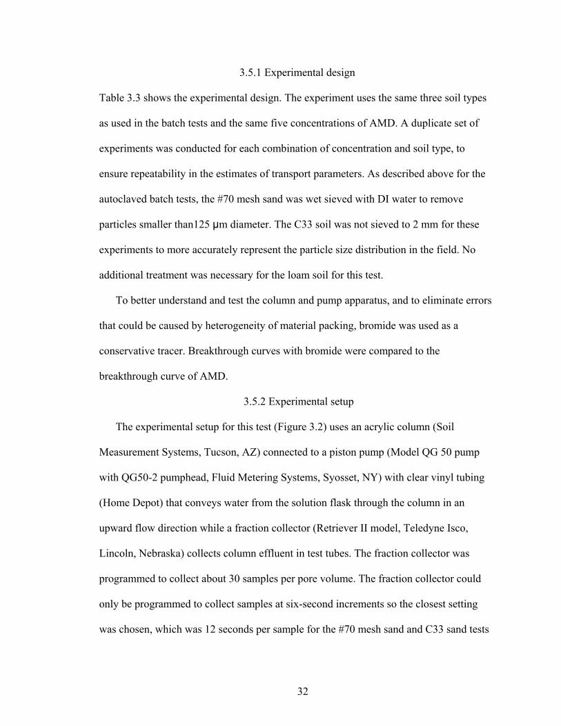
3.5.1 Experimental design
Table 3.3 shows the experimental design. The experiment uses the same three soil types
as used in the batch tests and the same five concentrations of AMD. A duplicate set of
experiments was conducted for each combination of concentration and soil type, to
ensure repeatability in the estimates of transport parameters. As described above for the
autoclaved batch tests, the #70 mesh sand was wet sieved with DI water to remove
particles smaller than125 μm diameter. The C33 soil was not sieved to 2 mm for these
experiments to more accurately represent the particle size distribution in the field. No
additional treatment was necessary for the loam soil for this test.
To better understand and test the column and pump apparatus, and to eliminate errors
that could be caused by heterogeneity of material packing, bromide was used as a
conservative tracer. Breakthrough curves with bromide were compared to the
breakthrough curve of AMD.
3.5.2 Experimental setup
The experimental setup for this test (Figure 3.2) uses an acrylic column (Soil
Measurement Systems, Tucson, AZ) connected to a piston pump (Model QG 50 pump
with QG50-2 pumphead, Fluid Metering Systems, Syosset, NY) with clear vinyl tubing
(Home Depot) that conveys water from the solution flask through the column in an
upward flow direction while a fraction collector (Retriever II model, Teledyne Isco,
Lincoln, Nebraska) collects column effluent in test tubes. The fraction collector was
programmed to collect about 30 samples per pore volume. The fraction collector could
only be programmed to collect samples at six-second increments so the closest setting
was chosen, which was 12 seconds per sample for the #70 mesh sand and C33 sand tests

33
Table 3.3: General setup for bromide/AMD column tests
Treatment Treatment type
Soil types #70 mesh
sand C33 sand
loam soil AMD concentrations (in ppb) 50 100 500 1000 5000 Number of soils 3 Number of concentrations 5 Number of tests 15 Number of pore volumes 3 Samples per pore volume 30 Samples per test 1350 Duplicate tests 1350 10% QA 270 Total number of samples 2970
Figure 3.2: Setup for the repacked column experiment
Piston Pump Fraction Collector
Soil Column
Solution

34
and 132 or 138 seconds per sample for the loam soil tests, depending on pumping rate.
The volume collected for each sample varied slightly, because the pumping rate varied
slightly during each experiment. A ½ mL aliquot of the collected sample was obtained
from the test tube and analyzed for AMD in the HPLC. The remainder of the sample was
then analyzed for bromide concentration with the specific ion electrode (model 720A
specific ion meter with Thermo Orion model 94-35 bromide electrode, Thermo Orion,
Beverly, Maryland).
The pumping rate was related to the saturated hydraulic conductivity of the soils, as
determined by Moran (2007). Using the flow rate from the soils section the pore water
velocity translated into mL/min in the column with a cross sectional area of 31.67 cm2 is
38.40 mL/min, 25.73 mL/min, and 2.99 mL/min for the #70 mesh sand, C33 sand, and
loam soil, respectively. Flow rates were set at approximately 24.6 mL/min for the tests
for the #70 mesh sand and C33 sand, and 3.0 mL/min for the tests for the loam soil (the
flow rate for the C33 sand is slightly less than the measured saturated hydraulic
conductivity due to limitations of the maximum flow rate for the pump). The exact
pumping rate for each test was determined for each column separately by collecting a
sample in a test tube for exactly one minute and weighing it to determine the mass of the
solution. The flow rate was then adjusted until the desired pumping rate was achieved.
The stability of the pumping rate either immediately before of after the tests was
determined by weighing a several pre-weighed test tubes and calculating the flow rate
during the test. The flow rate for all the tests never deviated from the original determined
flow rate during the test by more than a 0.08 mL/min (~0.33% of the total flow) for the

35
#70 mesh sand and C33 sand tests, or by more than 0.03 mL/min (~1.00% of the total
flow) for the loam tests.
In some cases, the sand-packed columns were used a single time, and then were
repacked, and in other cases, the sand-packed columns were used repeatedly. The
columns used for repeated experiments were flushed with at least 5 pore volumes of test
solution similar to Korom (2000) to remove all remaining bromide and AMD before the
next test was started. Laboratory analyses of bromide and AMD confirmed that levels
were below detection limits at the start of subsequent tests.
3.5.2.1 Test solution for column tests
The test solution used for the repacked column experiment was the same used by
Moran (2007). This solution is a 0.005 M CaSO4 (Fisher Scientific) test solution
augmented with 0.3gm/L thymol (J.T. Baker, Phillipsburg, Virginia) as an anti-microbial
agent. This is the standard test solution described by Klute and Dirksen (1986). This
solution was chosen to correlate the experiments from Moran (2007) but also because the
presence of cations is necessary for PAM to flocculate properly. The 0.005 M CaSO4
solution is equivalent to 200 ppm Ca+2 which correlates to the measurements in the canals
in PAM field scale tests (Susfalk et al., 2007). Those results showed that canal samples
contained 71, 196, and 234 ppm of Ca+2. In addition to Ca+2 the canal samples also
contained 22, 89, and 128 ppm of Mg+2, and 38, 189, and 294 ppm of Na+.
To make the test solution for the specific experiments, a concentrated stock solution
of AMD was made by mixing 50 mL of test solution and 250 mg of AMD, creating a
solution of 500 ppm. Then the necessary volume of the stock solution was added to the
volume of the test solution, using the equation:

36
2211 CVCV (9)
where V1 is the volume of the stock solution, C1 is the concentration of the stock solution,
V2 is the volume of the test solution and C2 is the concentration of the test solution.
Sodium bromide (EMD Chemicals) was then added to the test solution at a
concentration of 200 ppm of bromide for all tests, and was pumped simultaneously with
AMD. The concentration of bromide was in accordance with the measurement capacity
of the specific ion electrode which has a minimum detection limit of 1 ppm and a
maximum detection of over 80,000 ppm, though the company recommends at least a two-
order-of-magnitude range for calibration.
3.5.2.2 Soil column preparation
The column used in this experiment is part of a pressure cell apparatus (Figure 3.3)
with dimensions 7.62 cm (3 inch) outside diameter, 6.35 cm (2.5 inches) inside diameter,
15 cm (5.9 inches) in length. The tubing for the column is made of a non reactive acrylic
material.
The C33 sand and loam soil were packed to a target bulk density of 1.7 gm/cm3 and
1.5 gm/cm3, respectively, which are close to known field bulk densities in their natural
undisturbed soil environment. The bulk density chosen for the #70 mesh sand was also
kept at 1.7 gm/cm3.
Initial soil water contents were obtained by weighing 1000 gm of air-dried soil and
then placing it in an oven (Napco model 420, Fisher Scientific) for 105°C for 24 hours to
drive off residual moisture on the soil. The soil was then weighed again and the
gravimetric water content was then calculated as:
g = (mass moist soil – mass oven dry soil)/ (mass oven dry soil)

37
Figure 3.3: Soil column used for experiments
The initial gravimetric water contents of the #70 mesh sand, C33 sand, and loam soil
were between 0.0015 - 0.0017, 0.0024 - 0.0027, and 0.0081 - 0.0088 respectively. These
measurements correlated well with the study by Moran (2007), so the same mass of soil
was used to pack the columns. For the #70 mesh sand and C33 sand, a column packed to
a bulk density of 1.7 gm/cm3 required 807.6 gm of oven-dry soil. For the loam soil, a
column packed to a bulk density of 1.5 gm/cm3 required 712.58 gm of oven-dried soil. To
account for the mass of residual water in the air-dried soil, an additional 0.15%, 0.27%,
and 0. 87% of the oven-dried soil was added to the columns so the final weight of air-
dried soil used to pack the columns to their respective bulk densities was 808.8 gm, 809.8
gm, and 718.78 gm for the #70 mesh sand, C33 sand, and the loam soil.
Columns were packed using a water-packing technique, as used by Moran (2007).
This packing method produces no apparent layering or particle size segregation and led to
>96% saturation percentages for all column tests. To pack the columns, the outlet of a
funnel (Figure 3.4 A) filled with the predetermined amount of soil was placed into the

38
Figure 3.4: Pictures of (A) soil column funnel apparatus and (B) packing a column
column (Figure 3.4 B). A volume of test solution was added to the column, equivalent to
2 - 3 cm in height, soil was then swirled into the column until the soil was near the water
surface. Water was then added again and the process was repeated until the column was
filled. When packing was nearly complete, the column was lightly tapped to settle the soil
so that the final few grams could be added. Excess water was removed with a paper
towel, to ensure no spillage of the soil.
The porosity of each column can be determined by the equation:
100)1( s
b
p
pf (10)
A B

39
where f is the porosity, pb is the bulk density of the column, and ps is the standard particle
density of a mineral soil, assumed to be 2.65 gm/cm3 (Hillel, 1998). The porosity of the
#70 mesh sand, C33 sand, and the loam soil were determined to be 35.85%, 35.85%, and
43.40% respectively.
The pore volume is the product of the porosity and volume of the soil column, and
was calculated for the #70 mesh sand, C33 sand, and the loam soil to be 170.29 cm3,
170.29 cm3, and 206.15 cm3. The percent saturation for each column is the quotient of the
volumetric water content and pore volume. Pore volumes were determined for each
experiment based on the known mass of soil added to the column assembly, and dividing
by the volume of the column.
3.5.2.3 Pulse and step inputs for breakthrough curves
Two types of boundary conditions are used for the column flow-through experiments:
pulse and step inputs. A pulse experiment is conducted by pumping through a
predetermined amount of test solution (usually in pore volumes) containing a compound
of interest and then pumping through test solution without the chemical of interest to
leach the chemical from the column. Pulse breakthrough curves thus have both an
adsorption and desorption front. If a compound sorbs onto soil and then desorbs during
the leach phase of the experiment, the breakthrough curve exhibits a tailing effect. The
shape adsorption and desorption curves are used to determine the sorption isotherm. A
step experiment is conducted by continuously pumping test solution containing the
compound of interest through the column. A step experiment sometimes uses multiple
(and increasing) concentration steps, which thus yields multiple adsorption fronts
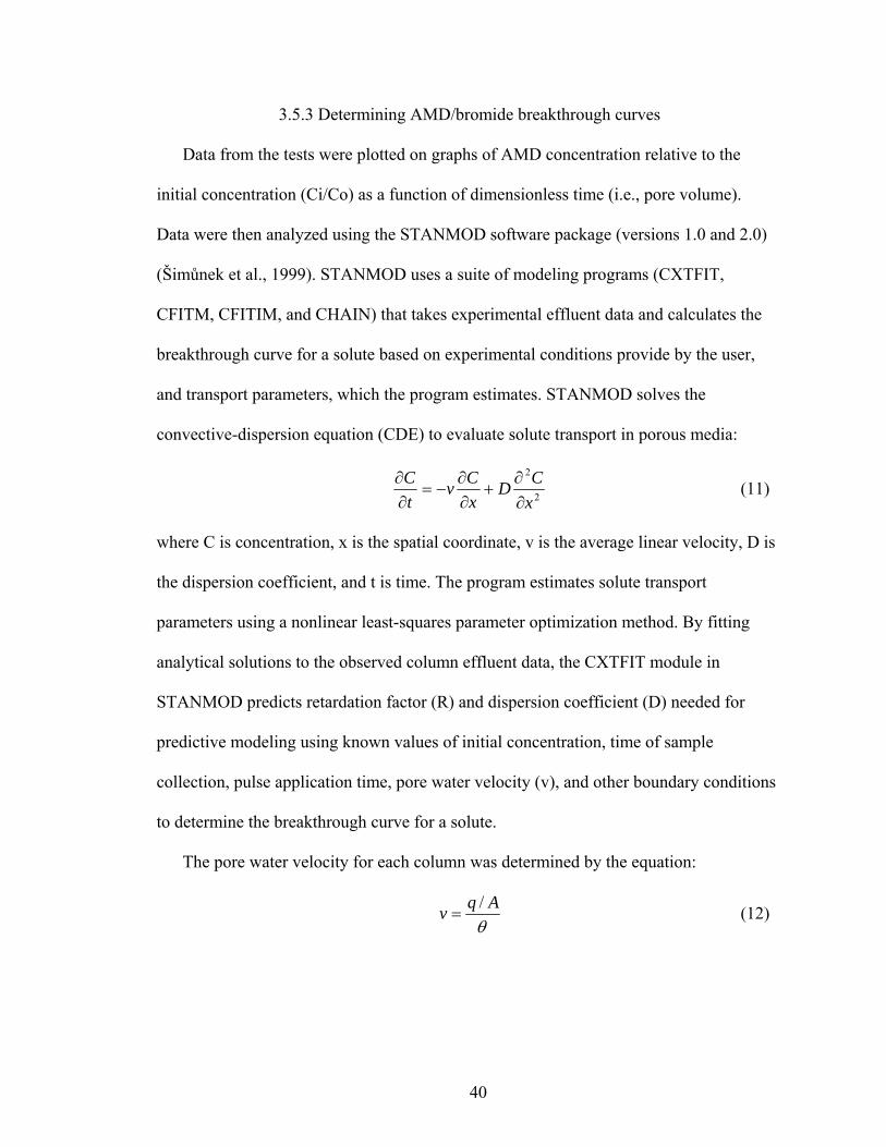
40
3.5.3 Determining AMD/bromide breakthrough curves
Data from the tests were plotted on graphs of AMD concentration relative to the
initial concentration (Ci/Co) as a function of dimensionless time (i.e., pore volume).
Data were then analyzed using the STANMOD software package (versions 1.0 and 2.0)
(Šimůnek et al., 1999). STANMOD uses a suite of modeling programs (CXTFIT,
CFITM, CFITIM, and CHAIN) that takes experimental effluent data and calculates the
breakthrough curve for a solute based on experimental conditions provide by the user,
and transport parameters, which the program estimates. STANMOD solves the
convective-dispersion equation (CDE) to evaluate solute transport in porous media:
2
2
x
CD
x
Cv
t
C
(11)
where C is concentration, x is the spatial coordinate, v is the average linear velocity, D is
the dispersion coefficient, and t is time. The program estimates solute transport
parameters using a nonlinear least-squares parameter optimization method. By fitting
analytical solutions to the observed column effluent data, the CXTFIT module in
STANMOD predicts retardation factor (R) and dispersion coefficient (D) needed for
predictive modeling using known values of initial concentration, time of sample
collection, pulse application time, pore water velocity (v), and other boundary conditions
to determine the breakthrough curve for a solute.
The pore water velocity for each column was determined by the equation:
Aqv
/ (12)

41
where v is the pore water velocity, q is the flow rate or discharge rate, A is the cross
sectional area of the column, and is the volumetric water content, which is this case is
the porosity.
Concentration for each sample was determined by converting the area response from
the HPLC using the calibration equation obtained as described in section 3.2. Bromide
sample concentration was estimated similarly by converting the millivolt response of the
specific ion electrode using the calibration equation. Samples of the test solution were
collected before the start of each test, and were analyzed for both bromide and AMD
concentration to determine the initial concentration. Each samples concentration was
divided by the initial concentration, yielding the relative concentration (Co/Ci), which
were used for the breakthrough curve analysis. The pore volume at the time of each
sample collection (i.e., used as dimensionless time) was obtained as the product of the
flow rate and the experimental time. The pulse length (in units of time) was multiplied by
the initial concentration to determine the mass of AMD and bromide pumped into the
column for each test. The percent recovery of each tracer was determined as the sum of
the individual masses of tracer collected in each sample (i.e., volume collected in each
sample times the concentration), divided by the total mass of solute added. The Co/Ci and
sample time data were entered into STANMOD and a predicted breakthrough curve was
fitted to the observed data using estimated values of retardation factor (R) and dispersion
coefficient (D). Values of dispersivity (α) were determined using the following equation:
vD / (13)
where v is the pore water velocity.

42
3.5.4 Determining AMD sorption
Methods developed by Burgisser et al. (1993) can then be used to determine the
sorption in the column experiments. To use this method, the hydrodynamic dispersion
coefficient (Ds) must be such that the peclet number is greater than 50, and the sorption
process must be at equilibrium. The peclet number is defined as Pe = Lv / Ds where L is
the length of the column and v is the pore water velocity. A peclet number greater than 50
indicates that the effects of dispersion are minimal and can be ignored (Burgisser et al.,
1993). If these two conditions are met, then the sorption for the column can be
determined by integrating the desorption front using the equation:
sC
pulse
ss dc
t
t
t
ct
pC
0 00
')1)'(
()1(
(14)
where Cs is the sorbed concentration of the chemical of interest, ps is the particle density
of the column, is the porosity of the column, t is the travel time from the first arrival of
the chemical, tpulse is the time duration of the pulse input, t0 is the average travel time
(length of the column divided by the pore water velocity) (Burgisser et al., 1993; Mon et
al., 2006).
3.6 Repacked bacteria inoculated column tests
The C33 sand and loam soil were inoculated with a known AMD-degrading
bacterium and degradation rates were tested using an AMD step concentration of 5 ppm.
Each test was conducted for about 10 pore volumes, at a flow rate of about 1 mL/min in
both soils. Blank tests were also conducted for each soil without inoculated bacteria, to
determine if the sterilization technique used between tests was efficient and effective.

43
Thirty samples per pore volume were taken for the first two pore volumes and fifteen
samples per pore volume for the last eight pore volumes. The extra sampling in the early
stages of the test gave a better resolution for the degree of AMD sorption on the step
breakthrough curve. Sampling for the latter part of the test was reduced to fifteen samples
to limit the waiting time from sample collection to sample analysis in the HPLC.
3.6.1 Experimental setup
The same experimental setup and column packing procedures used in the first set of
column tests was used for this test. Only the C33 sand and loam soil were used for these
experiments. Competing nitrogen sources were added to determine if competing nitrogen
would affect the ability of the bacteria to degrade AMD. Two types of bacteria were used
ones grown in media with 5 ppm AMD added so they would be experienced to degrading
AMD and ones grown in media with no added AMD so they would be naive to seeing
AMD. Additionally, the soils in this set of experiments were autoclaved using the same
method as described in Section 3.3 to ensure that the soil was sterilized of interfering
bacteria. Autoclavable tubing (Pharmed Masterflex silicone tubing, Cole-Parmer, Vernon
Hills, Illinois) was used instead of the clear vinyl tubing and sterilized after each test.
Sterilization of all components of the acrylic soil column and the pump head could not be
done by autoclaving because autoclaving would warp or melt of the acrylic and
negatively affect the ceramic. These pieces were instead soaked in an ethanol solution
and air dried to kill bacteria on the column components and pump apparatus to reduce or
preclude cross-contamination.

44
3.6.1.1 Test solution for column tests
The test solution was changed from that used in the first repacked columns, to ensure
that the bacteria would have a growth medium similar to a natural environment. A
solution of “flow through media” was made to achieve this. Several tests were conducted
in which AMD was the sole nitrogen source, and other tests were conducted in which a
competing source of nitrogen was added to determine whether the competing nitrogen
sources affected the amount of AMD degradation by the bacteria.
Flow through media was a modified form of the M1 medium (Myers and Nealson,
1988) with added calcium to replicate the sodium adsorption ratio (SAR) of the previous
test solutions. The modified test solution, called M1-SAR1 contains 340 mg of CaSO4,
112.3 mg Na2SO4 (Mallinckrodt Chemicals, Hazelwood, Missouri), 450 mg KH2PO4
(J.T. Baker), 1 gm K2HPO4 (J.T. Baker), 10ml of wolfs mineral solution (Wolin et al.,
1963), 0.4 mg NiSO46H2O (J.T. Baker), and 180mg glucose (Mallinckrodt Chemicals).
For the tests run with no competing nitrogen source, 5 ppm AMD was used as the
sole nitrogen source. In these cases, the nitrogen in the AMD is present at a concentration
of 1 ppm. In experiments with competing nitrogen, 1 ppm of total nitrogen was achieved
by adding KNO3 (J.T. Baker) and NH4Cl (Fisher Scientific) to the 1 ppm AMD.
3.6.1.2 Isolation and characterization of column test bacterium
Bacterium was isolated by enrichment culture technique using M1-SAR1 broth
shaken at room temperature. The isolated bacterium was taken from sediment sampled
from canals in Klamath Falls, Oregon.
A volume of 100 mL of the medium containing AMD and 1 gram of soil was grown
for 5 days, transferred, and isolated on M1-SAR1 agar plates. The ability of the

45
bacterium to degrade AMD was confirmed using HPLC analysis and; thus; the bacterium
to be utilized for future studies was determined.
3.6.2 Determining AMD degradation rate, percentage, and half-life
A predicted breakthrough curve from STANMOD without microbial degradation, and
based on experimental conditions used in the first set of column experiments was placed
on the same graph as the experimental data. This side-by-side comparison is a graphical
example of the degree of degradation that would occur without consideration of microbial
degradation. The degradation rate, half-life and total degradation percentage were
determined using the same procedure as outlined in Section 3.4.3.
3.7 Experiment 5: canal soil core column tests
3.7.1 Experimental design/setup
Canal soil cores were obtained from a field site in the Rocky Ford Highline canal,
which flows near Rocky Ford, Colorado. Three soil cores were taken from each of two
sites, one upstream where no PAM applications had taken place and another site 8.3 km
downstream of a PAM treated canal reach. Soil cores were collected using a method
similar to those described by Hendrickx and Dekker (2002). Here, an acrylic soil core
sampler was manually pushed into the canal surface and then removed with a small
shovel. Samples were stored at 4° C after collection until they were used in experiments.
The sampling cores (7.65 cm ID by 15 cm long) fit into the pressure cells directly without
any other modification. The flow through solution for this test was natural canal water,
which was filter sterilized (Nalgene 150 ml analytical filter unit 2 μL pore size, Nalge
Co., Rochester, New York) to remove bacteria.

46
The same experimental setup as described earlier was used for these tests, except that
soil cores from the upstream site were run at different AMD concentrations, one at 5 ppm
and the other at 1 ppm. The soil cores from the downstream site were conducted using
AMD at concentrations of 2.5 ppm and 1 ppm.
Bulk density of the soil was estimated by taking one of the three collected cores from
each site and determining the bulk density before the test. The estimated pore volume for
the column test for each site was then extrapolated from this. Pumping rate was kept at 1
mL/min. When the experiments were completed, the columns were disassembled and the
actual bulk density of the each core was independently determined.
3.7.2 Determining column degradation rate, half-life and percentage
As with the bacterial soil column tests the estimated breakthrough curve with no
microbial degradation was graphed with the experimental data. The soil in these tests is
different than the soils from the column tests, however since no batch experiments or
blanks could be run on these columns the no microbial degradation breakthrough curves
were estimated with the same parameters obtained for R and D from the soil column
tests. The degradation rate, half-life and total degradation percentage were determined
using the same procedure as outlined before.
3.8 Predictive numerical modeling with HYDRUS-2D
Numerical modeling was conducted to predict PAM and AMD migration in field
scenarios using the HYDRUS-2D program (version 1.0) (Šimůnek et al., 2006). The
HYDRUS- 2D program numerically solves the Richards' equation for variably saturated
water flow and convection-dispersion type equations for solute transport. Richards’

47
equation is a combination of the continuity equation and Darcy’s law. Richards’ equation
for one dimensional vertical flow is:
1z
h)h(K
zt
h)h(C
t
(15)
where t is time in days, C is the soil water capacity curve, h is the soil water pressure
head, K is the hydraulic conductivity of a soil, and z is the vertical distance. The
convective dispersion equation described in equation 11 is transformed into the two-
dimensional case in equation 16, and is modified to include processes of sorption and
decay or degradation:
Gy
CD
x
CD
y
Cv
x
Cv
t
C
C
Sb
2
2
2
2
1
(16)
where is the porosity, S is the solute concentration in sorbed phase, and G is a source-
sink term that represents the rate at which a solute will be removed from solution through
decay or degradation (van Genuchten et al. 1974: Šimůnek et al., 2006).
The data needed to run the model is the initial soil conditions, initial contaminant
concentration, retardation factor, sorption coefficient, and microbial/UV degradation
rates for AMD, and the hydraulic conditions in the canal environment (head level, depth
to groundwater, and knowledge of the boundary conditions).
The numerical model focused on the transport of AMD from the canal itself through
the partially saturated soil underneath the canal and downward to the water table. The
results from the laboratory studies and knowledge of flow conditions in earthen canals
were used to predict movement of AMD. Hydraulic properties for soil material used were
determined by the van Genuchten - Mualem equations (van Genuchten, 1980; Mualem,
1976) with no hysteresis. The governing equations for solute transport were solved using

48
the Crank – Nicholson time-weighting scheme, and Galerkin finite element space
weighting scheme. A pulse length of 5 days for AMD was chosen to reflect a maximum
time that PAM would release AMD by residual release. The models were run for 50 days.
The test design is listed in Table 3.4 and the finite element mesh and pressure heads are
shown in Figures 3.5a and b. Parameters for the van Genuchten equation were estimated
using the Rosetta software (Schaap et al., 1998) found in the HYDRUS-2D package. The
parameter specifically include residual soil water content (r), saturated soil water
content (s), and the two soil water retention factors , and n from the grain size analysis
of the #70 mesh sand, C33 sand, and the loam soil. The known Ksat for each of the three
soils described in Section 3.1 was used in lieu of the value provided by Rosetta.
The model was set up with no imposed gradient; causing the groundwater to have no
initial flow at the start of the simulation. Once the simulation begins and water seeps
from the canal, a water table mound is created and groundwater begins to move. Water
table gradients measured from a particular field site for other PAM-related studies were
not used for this modeling because of variability of field conditions. The soil material
was assumed to be homogeneous and isotropic. The PAM layer in the canal was specified
for nodes that connected with the canal surface and defined by modifying the van
Genuchten parameters (r, s, , and n) until they were similar to soils that possessed
Ksat values for soil treated with PAM at 5 and 10 lbs/ca. Both full and partial canal seals
were tested. To simulate a full and partial canal seal, nodes were assigned PAM-treated
soil properties from the bottom of the canal to approximately half a meter below the
water surface. Properties for untreated soil were assigned to the remainder of the canal
nodes. Depths to the water table were simulated by setting the pressure head value at

49
Table 3.4: Outline of HYDRUS test design
Treatment Treatment type
Soil type #70 mesh sand C33 sand loam soil
PAM conductivity levels 5 lbs/ca 10 lbs/ca
Water table level 0 meters 5 meters 10 meters
Full seal/ partial seal Full Partial
Figure 3.5A: Case study for PAM lined canal in the HYDRUS-2D program
Figure 3.5B: Pressure gradients for the canal with 5-meter water table depth
2 meters
10 M
25 M
observation nodes 1-7
full and partial seal “soils”
constant pressure boundary
free drainage boundary
water table at 5 m
gradient from 0 m to -1 m pressure head
increasing pressure with depth
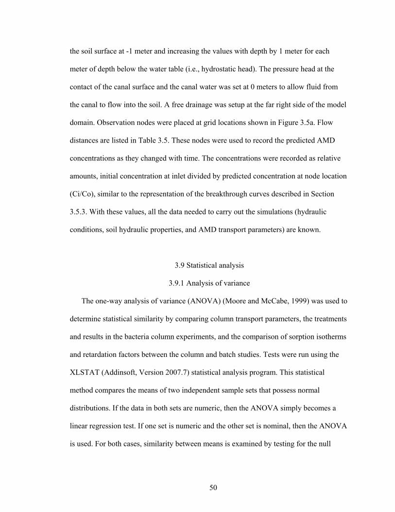
50
the soil surface at -1 meter and increasing the values with depth by 1 meter for each
meter of depth below the water table (i.e., hydrostatic head). The pressure head at the
contact of the canal surface and the canal water was set at 0 meters to allow fluid from
the canal to flow into the soil. A free drainage was setup at the far right side of the model
domain. Observation nodes were placed at grid locations shown in Figure 3.5a. Flow
distances are listed in Table 3.5. These nodes were used to record the predicted AMD
concentrations as they changed with time. The concentrations were recorded as relative
amounts, initial concentration at inlet divided by predicted concentration at node location
(Ci/Co), similar to the representation of the breakthrough curves described in Section
3.5.3. With these values, all the data needed to carry out the simulations (hydraulic
conditions, soil hydraulic properties, and AMD transport parameters) are known.
3.9 Statistical analysis
3.9.1 Analysis of variance
The one-way analysis of variance (ANOVA) (Moore and McCabe, 1999) was used to
determine statistical similarity by comparing column transport parameters, the treatments
and results in the bacteria column experiments, and the comparison of sorption isotherms
and retardation factors between the column and batch studies. Tests were run using the
XLSTAT (Addinsoft, Version 2007.7) statistical analysis program. This statistical
method compares the means of two independent sample sets that possess normal
distributions. If the data in both sets are numeric, then the ANOVA simply becomes a
linear regression test. If one set is numeric and the other set is nominal, then the ANOVA
is used. For both cases, similarity between means is examined by testing for the null

51
Table 3.5: Observation node properties
Observation node name Grid location Distance from source† -------------------------------- -------(x, z) meters------- -------meters------- Node 1 (2.5, -1.8) 0.92Node 2 (2.75, -4.75) 3.79Node 3 (2.75, -7.5) 6.46Node 4 (3, -10) 8.46Node 5 (10, -10) 12.22Node 6 (20, -10) 20.44Node 7 (25,-10) 25.04
† - Based on point-to-point measurements; not necessarily along flow lines
hypotheses (no difference in the means) or the alternative hypotheses (differences in the
mean exist). In essence, the ANOVA partitions the total sum of square differences into
components of model error and variance about the mean. If the null hypothesis is true
(i.e., no difference in the mean values), then the ratio of mean square of the model (MSG)
to the mean square error (MSE), or the F value, will be less than a critical value
determined from the degrees of freedom of the numerator (DFG) and the degrees of
freedom of the denominator (DFE). The DFG is determined by:
1 IDFG (17)
where I is the number of sample means tested. DFE is determined by:
INDFE (18)
where N is the total number of samples. Values of DFG and DFE determine the F critical
value, based on the level of confidence desired. All data analysis was done at a 95%
confidence (i.e., = 0.05) to determine the F critical value. Also, the P-value for each
test is determined to quantify the possibility that a higher F value would occur by chance.
Higher P-values indicate a higher confidence in the finding of similarity of means (i.e., a

52
P-value of 0.90 means a 90% chance that a calculated F value would be higher than the
critical F-value determined for the specific case).
3.9.2 Multiple comparison
In cases where the null hypothesis is rejected in the ANOVA, a multiple comparison
of sample means is conducted to determine which sets of data are similar and which sets
are statistically different from one another. The multiple comparisons were done by
computing the t statistics for all the pairs using the equation:
ji nnp
jiij s
xxt
11
(19)
where i and j are two different sample sets, xi and xj are the means of the sample sets, ni
and nj are the number of samples for each sample set, and sp is the pooled sample
standard deviation which is determined by:
)1(...)1()1(
)1(...)1()1(
21
2222
211
n
nnp nnn
snsnsns (20)
where s12 is the sample variance of a particular sample set. If the absolute values of tij
t*, which is determined from the multiple comparison procedure used to fit the the data,
then the means are statistically different. Tukey’s HSD (honestly significant difference)
test was used in this study as it is the most widely used test for multiple comparison
(Moore and McCabe, 1999). This test states that a t* value greater than 2.80 shows
statistical different.
3.9.3 ANCOVA statistical analysis
The data for the sorption studies was also analyzed using the two way analysis of
covariance (two-way ANCOVA) technique (Moore and McCabe, 1999) using the

53
XLSTAT (Addinsoft, Version 2007.7) statistical analysis program. This statistical
method is used when two independent variables (factors A and B) are being applied to a
dependant variable (ε). In this study for example, the experimental design has there is a
nominal independent variable (soil type), a numeric independent variable (AMD
concentration), and a numeric dependent variable (sorption). The test provides answers to
three questions: (1) Does the soil type affect sorption of AMD?; (2) Does the AMD
concentration affect sorption?; (3) Do certain soil types and AMD concentrations
together affect sorption?
If no interaction is found between the independent variables, then an additive model
can be used. The additive model is:
ijX jiijk (21)
where α is the effect of factor A, β is the effect of factor B, i is the number of A factors, j
is the number of B factors, k is the number of replications as each combination of factor
A and B, and ε is the dependent variable. To test this model, three null hypotheses are
posed and addressed based on laboratory data. The test solves the models for their F
statistics based on the sums of squares and the mean square quantities (Moore and
McCabe, 1999).
If interaction is found between the independent variables, then a model that allows for
interaction is used. This model is:
ijX ijjiijk (22)
where γij is the interaction between variables A and B. To test this model, four null
hypotheses were set up based on the data and solved for their F statistics based on the
sums of squares and the mean square quantities (Moore and McCabe, 1999). As

54
described above, a small F value with a high P value indicates that the sample means are
statistically similar. The results provide statistically validated relationships between the
sorptive characteristics of AMD, given the concentrations and soils used in the study, as
well as relationships between R and concentration and soils.
55
CHAPTER 4
DATA ANALYSIS
4.1 Soil physical properties
4.1.1 Particle size distribution
Particle size distributions of the fine-earth fraction (i.e., particle sizes < 2 mm) for the
three soil materials collected using the grab method are listed in Table 4.1. Table 4.2
provides the particle size analyses from samples that were also taken from bulk storage,
but that underwent autoclaving. The results (shown as differences in Table 4.3) illustrate
the very small changes in fine content (silt + clay), possibly due to autoclaving or just
random variability from collection in the storage buckets. In some cases, the fines content
increased, and other cases it decreased.
4.1.2 Surface area analysis
The results of the surface area analysis are shown in Table 4.4. The results for the wet
sieved #70 mesh sand versus the non-sieved sand show a 0.024-0.107 (6.4 - 28.7%)
decrease in total surface area after wet sieving, indicating that the fines were washed out
of the soil from wet sieving. The differences in the non-autoclaved material versus the
autoclaved material are 17.2%, -5.0%, -0.8% and -5.4% change in surface area for the
non-wet sieved #70 mesh sand, wet sieved 70 mesh sand, C33 sand, and loam soil
respectively. The lack of any observable trend of change in the soils supports the
conclusion that soils were not altered due to autoclaving.

56
Table 4.1: Particle size distributions of fine-earth fraction (< 2 mm) for three soil materials used in the research.
Type of soil Gravel Sand Silt Clay -%- -%- -%- -%- -%- -%- >2mm 1-2mm >62.5 um 15 um 3 um <3 um #70 mesh sand 0.00 0.00 97.50 1.30 0.20 0.90 C33 sand 0.00 24.50 72.20 1.10 1.10 1.20 loam soil 0.00 0.00 80.39 6.36 4.36 8.89
Table 4.2: Particle size analysis for C33 sand and loam soil autoclaved samples
Sample name Gravel Sand Silt Clay >2 mm >62.5 um 15 um 3 um <3 um - % - - % - - % - - % - - % - C33 sand-sample 1 no autoclaving 17.19 98.77 0.25 0.41 0.57C33 sand-sample 1 autoclaved 1 time 15.15 98.71 0.28 0.44 0.57C33 sand-sample 1 autoclaved 2 times 15.36 98.59 0.32 0.46 0.64C33 sand-sample 1 autoclaved 3 times 17.21 98.83 0.24 0.40 0.53C33 sand-sample 2 no autoclaving 18.22 98.39 0.30 0.56 0.75C33 sand-sample 2 autoclaved 1 time 15.40 86.89 2.88 4.27 5.96C33 sand-sample 2 autoclaved 2 times 15.21 98.62 0.00 0.40 0.97C33 sand-sample 2 autoclaved 3 times 13.02 98.79 0.25 0.44 0.51loam-sample 1 no autoclaving 0.00 80.39 6.36 4.36 8.89loam-sample 1 autoclaved 1 time 0.00 80.69 6.36 4.34 8.61loam-sample 1 autoclaved 2 times 0.00 81.30 5.75 4.26 8.69loam-sample 1 autoclaved 3 times 0.00 81.68 5.74 4.20 8.39loam-sample 2 no autoclaving 0.00 87.49 4.33 2.83 5.35loam-sample 2 autoclaved 1 time 0.00 80.85 6.31 4.29 8.56loam-sample 2 autoclaved 2 times 0.00 80.90 6.06 4.36 8.68loam-sample 2 autoclaved 3 times 0.00 81.42 5.77 4.15 8.66

57
Table 4.3: Change in grain size for C33 sand and loam from autoclaving cycles
Sample name Sand Silt Clay >62.5 um 15 um 3 um <3 um - % - - % - - % - - % - C33 sand-sample 1 autoclaved 1 time -0.06 0.03 0.03 0.00C33 sand-sample 1 autoclaved 2 times -0.18 0.07 0.05 0.07C33 sand-sample 1 autoclaved 3 times 0.06 -0.01 -0.01 -0.04C33 sand-sample 2 autoclaved 1 time -11.50 2.58 3.71 5.21C33 sand-sample 2 autoclaved 2 times 0.23 -0.30 -0.16 0.22C33 sand-sample 2 autoclaved 3 times 0.40 -0.05 -0.12 -0.24loam-sample 1 autoclaved 1 time 0.30 0.00 -0.02 -0.28loam-sample 1 autoclaved 2 times 0.91 -0.61 -0.10 -0.20loam-sample 1 autoclaved 3 times 1.29 -0.62 -0.16 -0.50loam-sample 2 autoclaved 1 time -6.64 1.98 1.46 3.21loam-sample 2 autoclaved 2 times -6.59 1.73 1.53 3.33loam-sample 2 autoclaved 3 times -6.07 1.44 1.32 3.31
Table 4.4: Surface area analysis
Sample name Surface area --m2/gm-- #70 mesh sand - no autoclaving 0.309 0.004 # 70 mesh sand - autoclaved 0.373 0.008 wet sieved #70 mesh sand - no autoclaving 0.285 0.007 wet sieved #70 mesh sand - autoclaved 0.266 0.007 C33 sand - no autoclaving 2.26 0.088 C33 sand - autoclaved 2.24 0.095 loam soil - no autoclaving 9.82 0.033 loam soil - autoclaved 9.29 0.027
4.1.3 Total organic content (TOC) analysis
The TOC for the #70 mesh sand was below the detection limit. The TOC in both the
C33 sand and the loam soil was 0.28%. The inorganic carbon in the soils was 0.49%,
2.28% and 5.46% for the #70 mesh sand, C33 sand, and loam soil, respectively. TOC was
also analyzed in the canal core samples and was shown to have values of 0.16% and
0.08% for the Site 1 columns and 0.24% for both Site 2 columns. Overall, the results

58
show that organic carbon contents were quite low in the soils tested, and therefore are not
expected to play a significant role in the sorption of AMD.
4.2 Experiment 1: AMD sorption batch tests
4.2.1 Sorptive characteristics of AMD
The analytical results are presented below in Tables 4.5 and 4.6 for un-autoclaved and
autoclaved soils, respectively. Results labeled as “False” indicate that sorption was not
statistically significant based on the detection limit for the HPLC analysis, and results
labeled as “True” were found to be significant. The results showed no significant sorption
of AMD onto C33 sand. In some cases (i.e., un-autoclaved soil with AMD concentrations
of 50 and 100 ppb) it appears that AMD concentrations were higher after the batch
studies, though changes in concentration were not significant. In the case of #70 mesh
sand, significant sorption was observed for material that did not undergo autoclaving.
Sorption was not significant after autoclaving. These differences are attributed to the wet
sieving that was done immediately prior to autoclaving. Thus, the differences are an
artifact of the experiment. This is confirmed by the surface size analysis presented in
section 4.1.2, which showed that the average surface area dropped by 28 percent due to
wet sieving the autoclaved soil. The amount of sorption in the #70 mesh sand was not
significant in the autoclaved, wet sieved samples. For the loam soil, sorption was found
to be significant at all concentrations tested, illustrating the importance of fine grained
fractions (silt and clay) in the sorption process. AMD sorption onto autoclaved loam soil
was observed to be higher than on untreated soil, but this is attributed to random
differences in the grab samples. The results from both sets of experiments (autoclaved
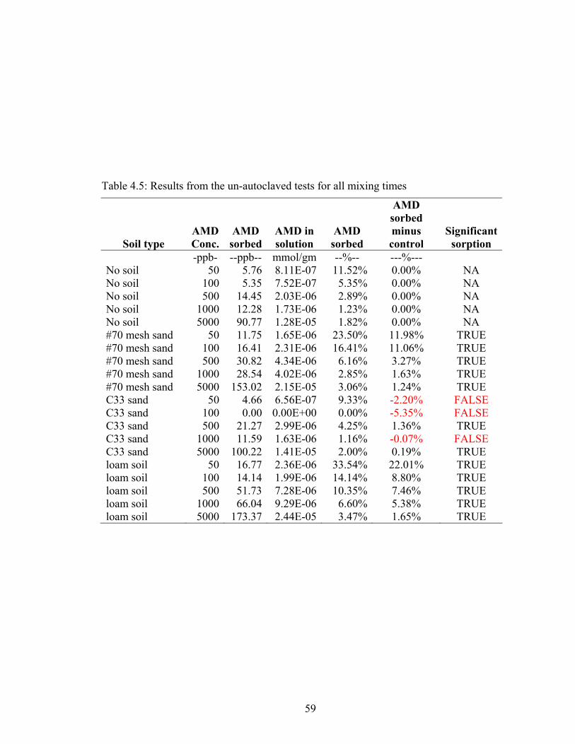
59
Table 4.5: Results from the un-autoclaved tests for all mixing times
Soil type AMD Conc.
AMD sorbed
AMD in solution
AMD sorbed
AMD sorbed minus control
Significant sorption
-ppb- --ppb-- mmol/gm --%-- ---%--- No soil 50 5.76 8.11E-07 11.52% 0.00% NA No soil 100 5.35 7.52E-07 5.35% 0.00% NA No soil 500 14.45 2.03E-06 2.89% 0.00% NA No soil 1000 12.28 1.73E-06 1.23% 0.00% NA No soil 5000 90.77 1.28E-05 1.82% 0.00% NA #70 mesh sand 50 11.75 1.65E-06 23.50% 11.98% TRUE #70 mesh sand 100 16.41 2.31E-06 16.41% 11.06% TRUE #70 mesh sand 500 30.82 4.34E-06 6.16% 3.27% TRUE #70 mesh sand 1000 28.54 4.02E-06 2.85% 1.63% TRUE #70 mesh sand 5000 153.02 2.15E-05 3.06% 1.24% TRUE C33 sand 50 4.66 6.56E-07 9.33% -2.20% FALSE C33 sand 100 0.00 0.00E+00 0.00% -5.35% FALSE C33 sand 500 21.27 2.99E-06 4.25% 1.36% TRUE C33 sand 1000 11.59 1.63E-06 1.16% -0.07% FALSE C33 sand 5000 100.22 1.41E-05 2.00% 0.19% TRUE loam soil 50 16.77 2.36E-06 33.54% 22.01% TRUE loam soil 100 14.14 1.99E-06 14.14% 8.80% TRUE loam soil 500 51.73 7.28E-06 10.35% 7.46% TRUE loam soil 1000 66.04 9.29E-06 6.60% 5.38% TRUE loam soil 5000 173.37 2.44E-05 3.47% 1.65% TRUE

60
Table 4.6: Results from the autoclaved tests for all mixing times
Soil type AMD Conc.
AMD sorbed
AMD in solution
AMD sorbed
AMD sorbed minus control
Significant sorption
-ppb- --ppb-- mmol/gm ---%--- ---%--- No soil 50 14.90 2.10E-06 29.81% 0.00% NA No soil 100 17.50 2.46E-06 17.50% 0.00% NA No soil 500 23.85 3.35E-06 4.77% 0.00% NA No soil 1000 22.52 3.17E-06 2.25% 0.00% NA No soil 5000 80.61 1.13E-05 1.61% 0.00% NA #70 mesh sand 50 10.50 1.48E-06 20.99% -8.82% FALSE #70 mesh sand 100 10.55 1.48E-06 10.55% -6.95% FALSE #70 mesh sand 500 8.58 1.21E-06 1.72% -3.05% FALSE #70 mesh sand 1000 0.00 0.00E+00 0.00% -2.25% FALSE #70 mesh sand 5000 63.61 8.95E-06 1.27% -0.34% FALSE C33 sand 50 13.30 1.87E-06 26.61% -3.20% FALSE C33 sand 100 16.82 2.37E-06 16.82% -0.67% FALSE C33 sand 500 32.75 4.61E-06 6.55% 1.78% TRUE C33 sand 1000 37.16 5.23E-06 3.72% 1.46% TRUE C33 sand 5000 117.64 1.65E-05 2.35% 0.74% TRUE loam soil 50 39.10 5.50E-06 78.20% 48.39% TRUE loam soil 100 36.03 5.07E-06 36.03% 18.53% TRUE loam soil 500 102.00 1.43E-05 20.40% 15.63% TRUE loam soil 1000 94.53 1.33E-05 9.45% 7.20% TRUE loam soil 5000 198.42 2.79E-05 3.97% 2.36% TRUE

61
and un-autoclaved) showed that mixing periods did not affect the amount of AMD
sorption onto soil materials (Figures 4.1 and 4.2), indicating that the sorption reactions
are instantaneous and not kinetically driven. The results also showed no substantial
difference in sorption between the autoclaved and un-autoclaved tests, indicating that the
reduction of AMD in solution was not influenced by microbial activity.
4.2.2 Sorption isotherms
The linear, Langmuir and Freundlich isotherms were all fitted to the data using the
correlation coefficient (R2) as a measure of fit to the sorption data (Table 4.7). The results
show that AMD sorption isotherms in all samples fit best to the Freundlich isotherm:
however, only the loam soil had a major affinity for the Freundlich isotherm. The #70
mesh sand and the C33 sand fit both Freundlich and liner well. The Freundlich isotherms
for the three significant tests are presented below with error for a 95% confidence
interval. Other test results found not to be significant are not shown below.
The Freundlich isotherm for the un-sieved un-autoclaved #70 mesh sand:
0870.0806.043 1003.11003.2 ws CC (23)
The Freundlich isotherm for the non autoclaved loam:
0631.0569.044 1032.21007.6 ws CC (24)
The Freundlich isotherm for the autoclaved loam:
0597.0372.054 1087.81027.2 ws CC (25)
The R values for the soils were determined using the Kd values obtained by fitting the
linear isotherm to the batch data. The values are presented in Table 4.8.

62
Hours
0 5 10 15 20 25
Cs
(mm
ol/g
)
0
1e-5
2e-5
3e-5
4e-5
5e-5No soil C33 soil#70 mesh sandLoam soil
Figure 4.1: Concentrations of AMD sorbed onto non-autoclaved soil
Hours
0 5 10 15 20 25
Cs
(mm
ol/g
)
0
1e-5
2e-5
3e-5
4e-5
5e-5No soilC33 soil#70 mesh sandLoam soil
Figure 4.2: Concentrations of AMD sorbed onto autoclaved soil

63
Table 4.7: Correlation coefficients for isotherms
Correlation Coefficients
Soil type Linear Langmuir Freundlich
Un-Autoclaved #70 mesh sand 0.8478 0.7065 0.8577
Autoclaved #70 mesh sand 0.5599 0.5178 0.5790
Un-Autoclaved C33 sand 0.6891 0.6409 0.7036
Autoclaved C33 sand 0.5211 0.5312 0.5884
Un-Autoclaved loam soil 0.7038 0.7511 0.8045
Autoclaved loam soil 0.1864 0.5016 0.5408
Table 4.8: Estimated retardation values
Soil type Kd b
Water
content ()
Retardation
Factor
--------------------- -------- g / cm3 ---%--- -----------------
Un-Autoclaved #70 mesh sand 5.0910-3 1.7 0.3585 1.024
Autoclaved #70 mesh sand 0† 1.7 0.3585 1.000
Un-Autoclaved C33 sand 0† 1.7 0.3585 1.000
Autoclaved C33 sand 0† 1.7 0.3585 1.000
Un-Autoclaved loam soil 6.3110-3 1.5 0.4340 1.022
Autoclaved loam soil 6.0510-3 1.5 0.4340 1.020
† - indicates that determined sorption coefficients are not significant
The linear isotherm for the non-autoclaved #70 mesh sand:
43 1054.41009.5 sC (26)
The linear isotherm non-autoclaved loam:
43 1091.41031.6 sC (27)
The linear isotherm autoclaved loam:

64
43 1085.81005.6 sC (28)
4.3 Experiment 2: AMD degradation flask study
4.3.1 Flask degradation rates
Estimated degradation and AMD half lives for the flask tests are shown in Table 4.9
and the graph of the degradation rate fits is shown in Figure 4.3. The test with the fastest
degradation rate was the Closed-Air Open-Light tests. The two samples open to light are
the highest and lowest in degradation indicating that light, at least at the wavelengths
found in the laboratory, had no definitive effect on AMD degradation. Also the samples
closed to air were found to have the two fastest degradation rates. This leads to the
conclusion that having the samples open to air also has no definitive effect on the
degradation of AMD. One possible explanation for the faster AMD degradation in closed
air samples is the potential of contamination from bacteria during sampling. Determining
similarity of degradation rates could not be done because of the lack of replicates and
samples.
The results show a large difference in the degradation rates between the Open-Air
Open-Light test and the Closed-Air Open-Light test. Degradation rates for the other two
treatments were within two standard deviations from the mean of the group of samples.
Results were similar for the half lives as well. The small sample size and large
differences limit the type of statistical analyses that can be performed on the data. The
results indicate that AMD is stable at room temperatures for a long time, thus confirming
that holding times for HPLC analysis (on the order of 12-24 hours) were not an
influencing factor for sample analysis.

65
Table 4.9: Estimated flask degradation values
Test Degradation rate constant
Final degradation Half life
-----hours-1----- --------%-------- ----days---- Open Air Open Light 2.17E-03 26.12 319 Open Air Closed Light 4.06E-03 58.95 171 Closed Air Open Light 1.03E-02 94.79 67 Closed Air Closed Light 6.50E-03 76.09 107
Time (in days)
0 50 100 150 200
N(t
) / N
0
0.0
0.1
0.2
0.3
0.4
0.5
0.6
0.7
0.8
0.9
1.0
1.1
Open air open lightOpen air closed lightClosed air open lightClosed air closed light
Figure 4.3: Graph of flask data and degradation rates (symbols are observed data, lines are fitted degradation rates)
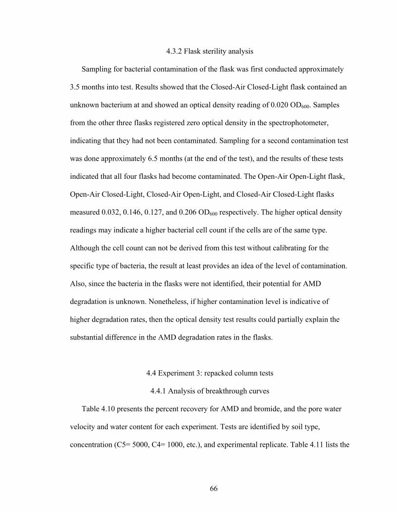
66
4.3.2 Flask sterility analysis
Sampling for bacterial contamination of the flask was first conducted approximately
3.5 months into test. Results showed that the Closed-Air Closed-Light flask contained an
unknown bacterium at and showed an optical density reading of 0.020 OD600. Samples
from the other three flasks registered zero optical density in the spectrophotometer,
indicating that they had not been contaminated. Sampling for a second contamination test
was done approximately 6.5 months (at the end of the test), and the results of these tests
indicated that all four flasks had become contaminated. The Open-Air Open-Light flask,
Open-Air Closed-Light, Closed-Air Open-Light, and Closed-Air Closed-Light flasks
measured 0.032, 0.146, 0.127, and 0.206 OD600 respectively. The higher optical density
readings may indicate a higher bacterial cell count if the cells are of the same type.
Although the cell count can not be derived from this test without calibrating for the
specific type of bacteria, the result at least provides an idea of the level of contamination.
Also, since the bacteria in the flasks were not identified, their potential for AMD
degradation is unknown. Nonetheless, if higher contamination level is indicative of
higher degradation rates, then the optical density test results could partially explain the
substantial difference in the AMD degradation rates in the flasks.
4.4 Experiment 3: repacked column tests
4.4.1 Analysis of breakthrough curves
Table 4.10 presents the percent recovery for AMD and bromide, and the pore water
velocity and water content for each experiment. Tests are identified by soil type,
concentration (C5= 5000, C4= 1000, etc.), and experimental replicate. Table 4.11 lists the

67
transport parameters estimated from each of the breakthrough curve experiments
(Appendix I graphs the fitted and modeled data for each experiment). Solute recoveries
tended to be consistently between 95% and 100% for all three soils. Mean recoveries for
#70 mesh sand, C33 sand, and loam soil were 96.17 %, 97.79 %, and 92.27 %
respectively. Values across all three soil types ranged from 81.61% - 105.26%, with the
lowest recovery values in the low concentration loam soils.
Data from the column tests shows that the R values for AMD are close to unity for
every test for every soil type (ranging from 0.98-1.06), indicating that AMD is a
conservative compound. Because the diffusion coefficient for AMD and bromide are so
low, 1.4 10-11 cm2 / s, and 1.0 10-9 cm2 / s respectively (Blaya et al., 2004 and
Maloszewski et al., 1998), the diffusion coefficient was considered to be insignificant.
Values of D and were then used to determine if dispersion in the different soils was
similar.
Using ANOVA, multiple comparison tests, and ANCOVA analyses, R, D, , and
percent recovery were tested for similarity for all initial concentrations and soil types.
The F-values, F-critical values, and P-values for all the ANOVA and ANCOVA analysis
are shown in Table 4.12 and the multiple comparison T-values and P-values are listed in
Table 4.13. Test results show that R for AMD is similar for all soil types and
concentrations. The D values, however, were determined to be statistically different.
Multiple comparison tests were done to determine which soil led to differences in D. The
results showed that #70 mesh sand, C33 sand, and the loam soil were all significantly
different from each other, indicating that the different grain size distributions in the soils
are causing differences in the flow characteristics in the columns. Initial concentrations

68
Table 4.10: Recovery and experimental conditions for soil column experiments
Experiment AMD recovery Br recovery Pore water
velocity Water
content () ------------- --------%-------- -------%------- ---cm3/min---- ----%----
#70 sand, C5-1 93.65 93.33% 2.17 36.96 #70 sand, C5-2 95.95 92.77% 2.16 37.04 #70 sand, C4-1 96.91 91.59% 2.14 36.88 #70 sand, C4-2 96.52 96.38% 2.18 37.99 #70 sand, C3-1 98.97 93.79% 2.16 37.92 #70 sand, C3-2 94.31 94.16% 2.14 38.07 #70 sand, C2-1 93.29 92.31% 2.07 37.30 #70 sand, C2-2 97.39 94.46% 2.05 37.43 #70 sand, C1-1 98.87 97.82% 2.01 39.14 #70 sand, C1-2 95.86 94.53% 2.01 38.88 C33 sand, C5-1 96.30 94.25% 2.05 40.12 C33 sand, C5-2 96.46 90.29% 2.28 35.58 C33 sand, C4-1 97.09 92.91% 2.10 39.26 C33 sand, C4-2 105.26 92.17% 2.24 35.91 C33 sand, C3-1 98.69 96.51% 2.22 36.16 C33 sand, C3-2 101.03 101.20% 2.19 36.56 C33 sand, C2-1 91.76 98.21% 2.04 37.96 C33 sand, C2-2 94.90 93.84% 2.12 36.11 C33 sand, C1-1 98.54 95.81% 2.09 36.54 C33 sand, C1-2 97.86 95.55% 2.13 36.41 loam, C5-1 99.83 96.31% 0.23 40.94 loam, C5-2 93.88 89.60% 0.24 41.82 loam, C4-1 100.90 96.78% 0.23 42.02 loam, C4-2 95.65 93.60% 0.22 42.95 loam, C3-1 93.40 97.21% 0.23 41.87 loam, C3-2 89.92 96.80% 0.23 42.57 loam, C2-1 81.61 93.26% 0.22 42.07 loam, C2-2 93.72 95.08% 0.22 42.52 loam, C1-1 85.51 98.85% 0.22 42.71 loam, C1-2 88.29 98.91% 0.23 40.69

69
Table 4.11: Estimated transport parameters for the soil column test
Retardation
Factor Dispersion Coefficient Dispersivity Experiment AMD Br AMD Br AMD Br
---------- ------- ------- cm2 / sec cm2 / sec cm cm #70 sand, C5-1 1.03 1.02 2.41E-02 2.10E-02 0.67 0.58#70 sand, C5-2 1.02 1.01 3.55E-02 3.98E-02 0.99 1.11#70 sand, C4-1 1.02 0.99 2.99E-02 2.83E-02 0.84 0.79#70 sand, C4-2 0.99 1.00 2.29E-02 1.74E-02 0.63 0.48#70 sand, C3-1 1.00 0.99 2.53E-02 2.09E-02 0.70 0.58#70 sand, C3-2 0.98 0.98 3.64E-02 3.19E-02 1.02 0.89#70 sand, C2-1 1.03 1.04 2.11E-02 2.84E-02 0.61 0.82#70 sand, C2-2 1.02 1.02 2.72E-02 2.78E-02 0.80 0.81#70 sand, C1-1 1.03 1.06 2.84E-02 4.60E-02 0.85 1.37#70 sand, C1-2 1.02 1.07 3.55E-02 5.83E-02 1.06 1.74C33 sand, C5-1 1.00 0.98 7.95E-02 6.95E-02 2.33 2.03C33 sand, C5-2 1.04 1.06 8.25E-02 5.89E-02 2.17 1.55C33 sand, C4-1 1.00 1.03 4.50E-02 5.48E-02 1.29 1.57C33 sand, C4-2 1.02 1.04 7.41E-02 6.17E-02 1.98 1.65C33 sand, C3-1 1.05 1.04 5.74E-02 3.56E-02 1.56 0.96C33 sand, C3-2 1.00 0.98 6.03E-02 4.96E-02 1.65 1.36C33 sand, C2-1 1.05 0.99 3.50E-02 5.40E-02 1.03 1.59C33 sand, C2-2 1.00 0.96 3.71E-02 3.12E-02 1.05 0.88C33 sand, C1-1 1.06 1.05 2.68E-02 3.01E-02 0.77 0.86C33 sand, C1-2 1.01 0.97 1.03E-01 4.53E-02 2.89 1.28loam, C5-1 1.03 0.92 4.46E-03 4.35E-03 1.16 1.13loam, C5-2 1.02 0.97 5.31E-03 3.99E-03 1.32 0.99loam, C4-1 1.07 0.96 6.92E-03 4.41E-03 1.81 1.15loam, C4-2 1.03 0.96 4.41E-03 6.14E-03 1.19 1.65loam, C3-1 1.01 0.95 2.46E-03 2.67E-03 0.64 0.70loam, C3-2 0.99 0.96 3.43E-03 5.03E-03 0.91 1.33loam, C2-1 1.00 0.90 1.03E-02 7.75E-03 2.81 2.11loam, C2-2 1.02 0.90 4.91E-03 5.81E-03 1.36 1.60loam, C1-1 1.02 0.93 3.13E-03 4.10E-03 0.86 1.13loam, C1-2 0.99 0.94 2.97E-03 4.36E-03 0.79 1.16

70
of AMD had no affect the dispersion coefficient. The values in all soils were
determined to be statistically different. Multiple comparisons showed that the #70 mesh
sand and the C33 sand were significantly different, but the C33 sand versus loam soil and
the #70 mesh sand versus loam tests proved to be similar; however, the P value for both
these comparisons was very low, indicating a statistically significant effect of only
when comparing results from the #70 mesh and the C33 sands. The in all initial
concentrations of AMD was determined to be similar. The percent recoveries for AMD in
all soils were determined to be statistically different. Multiple comparison tests showed
different recoveries between the C33 sand and the loam soil, while the other comparisons
were similar. These results indicate a lower than expected recovery for the loam soil
compared to recoveries in the C33 sand (recovery in the #70 mesh sand was similar to the
loam soil). Low recovery in the loam could be due to several factors, including possible
bacterial contamination of the loam soil, causing a small amount of degradation, a small
amount of chemical breakdown in the AMD due to the presence of charged clay particles
in the loam soil or possible error in the determination of the AMD peak in the HPLC due
to fine clays interfering with the integration. Initial concentration had no effect on the
percent recoveries, although the low P value for this test shows a possible trend.
4.4.2 Column sorption isotherms
All column peclet numbers were determined to be greater than 300, which is much
greater than the 50 needed, which confirms that the methods in Section 3.5.4 can be used
to analyze the column tests for sorption. The individual values of sorption for each
concentration level were then plotted in Tablecurve and fitted to different forms of
sorption isotherms to determine which form fit the data most closely.

71
Table 4.12: ANOVA and ANCOVA statistics for AMD parameter comparisons
Test F-value F-Critical
value P-value Effect ANOVA - AMD R vs. soil type 0.389 3.710 0.681 NOANOVA - AMD R vs. initial concentration 0.331 3.330 0.570 NOANCOVA - AMD R vs. soil type vs. concentration 0.358 NA† 0.784 NOANOVA - AMD D vs. soil type 36.184 3.710 0.0001 YESANOVA - AMD D vs. initial concentration 0.246 3.330 0.909 NOANOVA - vs. soil type 6.277 3.710 0.006 YESANOVA - vs. concentration 0.231 3.330 0.918 NOANOVA - AMD percent recoveries vs. soil type 4.506 3.710 0.020 YESANOVA - AMD percent recoveries vs. concentration 1.822 3.330 0.156 NO
†NA- ANCOVA tests do not have F-critical values
Table 4.13: Multiple comparison statistics for parameter comparisons
Test T-value T-test
P-value Effect MC test- AMD D in #70 mesh sand vs. C33 sand 8.408 0.0001 YESMC test- AMD D in #70 mesh sand vs. loam soil 4.824 0.0001 YESMC test- AMD D C33 sand vs. loam soil 3.656 0.0003 YESMC test- AMD in #70 mesh sand vs. C33 sand 3.538 0.004 YESMC test- AMD in #70 mesh sand vs. loam soil 1.934 0.261 NOMC test- AMD C33 sand vs. loam soil 1.604 0.149 NOMC test- AMD percent recovery in #70 mesh sand vs. C33 sand 0.856 0.6720 NOMC test- AMD percent recovery in #70 mesh sand vs. loam soil 2.064 0.1160 NOMC test- AMD percent recovery C33 sand vs. loam soil 2.920 0.0190 YES

72
Similar to results found for the batch experiments, the linear and Freundlich isotherms
provided good fits to the data (Table 4.14). The Freundlich isotherms for the tests are
presented below with error for a 95% confidence interval.
The Freundlich isotherm for the #70 mesh sand:
0042.0009.132 1030.11024.5 ws CC (29)
The Freundlich isotherm for the C33 sand:
0157.0026.132 1062.51000.6 ws CC (30)
The Freundlich isotherm for the loam soil:
0274.0109.132 1026.21035.1 ws CC (31)
4.4.2 Comparing batch and column sorption isotherms and retardation values
Parameters in the sorption isotherms calculated in the batch studies are less than those
calculated in the column tests for all soils; however, when the three significant sorption
isotherms from the batch studies were compared to the three isotherms from the column
studies using ANOVA statistical analysis, they were determined to be statistically similar
(F < F critical = 0.414 < 9.55 P = 0.636) for batch isotherms versus column isotherms.
This test was conducted on only 3 samples for each set and this may induce error into the
test, but given that there are no experimental outliers in the transport parameters that were
identified from the data, the three randomly-sampled values used in the comparison
should be valid.
The mean values for R for the batch studies were compared to those obtained from
the column tests. The R values were 1.024, 1.000, and 1.022 for batch studies and 1.014,
1.023, and 1.018 for the column tests, using for the #70 mesh sand, C33 soil and the loam
soil respectively. This shows good correlation between the two experimental methods.

73
Table 4.14: Correlation coefficients for isotherms
Correlation Coefficients
Soil type Linear Freundlich
#70 mesh sand 0.9999 0.9999
C33 sand 0.9976 0.9976
loam soil 0.9974 0.9959
4.5 Experiment 4: bacteria inoculated repacked column tests
4.5.1 Breakthrough curve analysis
Data used in the breakthrough curve analysis were obtained using the same methods
as described in section 4.3.1. Specifically, the experiments yielded AMD concentration
with time. Using column parameters as described earlier (i.e., pore water velocity, initial
concentration, etc.) for each experiment, STANMOD was used to predict the
breakthrough curve, assuming no degradation. Experiments were varied by soil, absence
or presence of competing nitrogen and type of bacteria. These graphs are shown in
Figures 4.4 A-J. The experiments are labeled by soil type, competing nitrogen (N+ for
competing nitrogen added, N- for no competing nitrogen), and the type of bacteria (e for
experienced, n for naïve, and x for no bacteria).
4.5.2 Bacteria column degradation rates and half lives
Estimated degradation rates and half-lives for the column tests are shown in Table
4.15. The final degradation percentage is calculated as ([1 – Co/Ci]*100%), which is a
measure of the concentration of AMD in the final sample taken for each test. This
parameter is essentially a gauge for the effectiveness of the bacteria at degrading AMD
after a three-hour contact period in the column. Note that the degradation rates are much

74
Pore Volume
0 2 4 6 8 10 12
Ci/C
o
0.0
0.2
0.4
0.6
0.8
1.0
AMDEstimated no degradation
A
Pore Volume
0 2 4 6 8 10
Ci/C
o
0.0
0.2
0.4
0.6
0.8
1.0
AMDEstimated no degradation
B
Figure 4.4: Graphs of (A) bacterial column tests with C33 sand and experienced bacteria without competing nitrogen, and (B) with competing nitrogen

75
Pore Volume
0 2 4 6 8 10
Ci/C
o
0.0
0.2
0.4
0.6
0.8
1.0
AMDEstimated no degradation
C
Pore Volume
0 2 4 6 8 10
Ci/C
o
0.0
0.2
0.4
0.6
0.8
1.0
AMDEstimated no degradation
D
Figure 4.4: Graphs of (C) bacterial column tests with C33 sand and naïve bacteria without competing nitrogen, and (D) with competing nitrogen

76
Pore Volume
0 2 4 6 8 10
Ci/C
o
0.0
0.2
0.4
0.6
0.8
1.0
AMDEstimated no degradation
E
Pore Volume
0 2 4 6 8 10
Ci/C
o
0.0
0.2
0.4
0.6
0.8
1.0
AMDEstimated no degradation
F
Figure 4.4: Graphs of (E) bacterial column tests with loam soil and experienced bacteria without competing nitrogen, and (F) with competing nitrogen

77
Pore Volume
0 2 4 6 8 10
Ci/C
o
0.0
0.2
0.4
0.6
0.8
1.0
AMDEstimated no degradation
G
Pore Volume
0 2 4 6 8 10
Ci/C
o
0.0
0.2
0.4
0.6
0.8
1.0
AMDEstimated no degradation
H
Figure 4.4: Graphs of (G) bacterial column tests with loam soil and experienced bacteria without competing nitrogen, and (H) with competing nitrogen

78
Pore Volume
0 2 4 6 8 10
Ci/C
o
0.0
0.2
0.4
0.6
0.8
1.0
AMDEstimated no degradation
I
Pore Volume
0 2 4 6 8 10
Ci/C
o
0.0
0.2
0.4
0.6
0.8
1.0
AMDEstimated no degradation
J
Figure 4.4: Graphs of (I) bacterial column tests with C33 sand, no bacteria, without competing nitrogen, and (J) loam soil, no bacteria, without competing nitrogen

79
Table 4.15: Degradation parameters for bacterial column tests
Test λ Recovery Final degradation Half-life Half-life--------------- --hours-1-- ----%---- --------%--------- --hours-- --days-- C33, N-, e 2.31E-01 4.98 100.00 3.01 0.13C33, N+, e 2.62E-01 3.61 100.00 2.64 0.11C33, N-, n 4.16E-01 2.13 100.00 1.67 0.07C33, N+, n 4.90E-01 1.80 100.00 1.41 0.06C33, N-, x 1.34E-03 99.60 15.00 518.05 21.59Loam, N-, e 7.74E-01 0.21 100.00 0.90 0.04Loam, N+, e 6.81E-01 0.31 100.00 1.02 0.04Loam, N-, n 2.97E-01 6.03 96.20 2.33 0.10Loam, N+, n 2.22E-01 23.03 95.20 3.12 0.13Loam, N-, x 3.90E-02 53.59 90.90 17.77 0.74
higher than were seen in the flask tests. Half lives for all tests including bacteria were less
than 3.5 hours indicating very rapid utilization of AMD.
ANOVA tests were used to analyze the competing nitrogen, bacteria type, and soil
type effect on degradation rate and half life. No multiple comparison tests were needed.
The results are presented in Table 4.16 and show that presence or absence of competing
nitrogen sources did not have a statistically significant effect on the degradation rate or
half life. Also bacteria type and soil type did not affect the AMD degradation rates or half
life. These results indicate that the competing nitrogen did not slow down or accelerate
the degradation rate of AMD. Bacteria that have utilized AMD before were no more
efficient at degrading the AMD than naïve cultures, and the differences between
experienced and naïve bacteria had no effect on the ability of the bacteria to utilize AMD.
One observed trend that naive bacteria appear to degrade AMD more effectively in the
C33 sand, and the experienced bacteria appear to degrade AMD better in the loam soil.
The blank tests for the C33 sand and loam soil show that the column apparatus was

80
Table 4.16: Results of ANOVA analyses for parameter comparisons
Test F-value F-Critical
value P-value Effect Competing nitrogen vs. degradation rate 0.009 6.940 0.926 NOCompeting nitrogen vs. half life 0.012 6.940 0.916 NOBacterial type vs. degradation rate 0.730 6.940 0.729 NOBacterial type vs. half life 0.132 6.940 0.426 NOSoil type vs. degradation rate 0.911 6.940 0.377 NOSoil type vs. half life 0.268 6.940 0.623 NO
properly sterilized between tests, as seen by the close match between experimental and
estimated concentrations.
4.5.3 Bacterial and competing nitrogen analysis
Bacterium used in the column tests was determined by 16S RNA gene sequencing
(Nevada Genomics Center, Reno, Nevada) to be Pseudomonas putida (gene sequencing
work was done by Labahn (2007) as part of the collaborative PAM study). These tests
also show that the concentration of bacterial cells in the bacteria column tests were about
1012 cells per gram of soil, a much higher concentration than was analyzed from samples
collected at other field sites (not related to this thesis). The bacteria in these tests were
grown with nutrient media and inoculated for 24 hours, allowing them to thrive in the
column.
Labahn (2007) analyzed the total ammonia and nitrogen for the column tests
conducted with competing nitrogen sources. These samples were taken during the
experiments at 2.5, 5, 7.5 and 10 pore volumes. Labahn (2007) showed that bacteria were
able to fully utilize the nitrogen added to the column through the growth media, and that
the ammonia added to the column through the growth media and the ammonia created

81
from AMD degradation were both partially utilized. The total ammonia concentration
never exceed 1 ppm, which indicates that the added ammonia was degraded at a rate
faster than ammonia was created by AMD degradation. The ammonia from both sources
(added and produced from AMD degradation) however, could not be discriminated.
4.6 Experiment 5: canal soil core column tests
4.6.1 Breakthrough curve analysis
The data for AMD concentration, Co / Ci, and pore volume was determined as
described in section 4.3.1. The graphs for the breakthrough curves are presented in Figure
4.5 A-D. During the Site 2 Column 2 experiment, concentration of AMD was increased
from 1 ppm to 5 ppm, which explains the increase in AMD concentration observed in the
breakthrough curve. AMD concentration was increased because no AMD degradation
was observed at the lower concentration, and it was believed that a higher concentration
could possibly “activate” the bacteria.
4.6.2 Canal column degradation rates
Estimated degradation rates and half-lives for the canal column tests are shown in
Table 4.17. The degradation rates observed in these tests were lower than observed in the
bacteria columns using the C33 sand and loam soil. This decrease in AMD degradation is
due to the lower concentration of active cells in the column, which is more indicative of
field conditions. However, even at these lower concentrations, the bacteria were still able
to degrade AMD at half-lives ranging from 30 – 42 hours except in the Site 2 – Column 2
test. The AMD degradation rates for the other three columns all have degradation rates

82
Pore Volume
0 2 4 6 8 10
Ci/C
o
0.0
0.2
0.4
0.6
0.8
1.0AMDA
Pore Volume
0 2 4 6 8 10
Ci/C
o
0.0
0.2
0.4
0.6
0.8
1.0AMDB
Figure 4.5: Graphs of (A) bacterial soil core column tests Site 1 – Column 1, and (B) Site 1 – Column 2

83
Pore Volume
0 2 4 6 8 10 12 14 16
Ci/C
o
0.0
0.2
0.4
0.6
0.8
1.0AMDC
Pore Volume
0 2 4 6 8 10 12 14 16
Ci/C
o
0.0
0.2
0.4
0.6
0.8
1.0
1.2D
Figure 4.5: Graphs of (C) bacterial soil core column tests Site 2 – Column 1, and (D) Site 2 – Column 2

84
Table 4.17: Degradation parameters for bacterial column tests
Test λ Percent recovery
Final degradation Half-life Half-life
-------------------- --hours-1-- ----%---- -------%-------- --hours-- --days-- Site 1 - Column 1 2.33E-02 64.71 41.50 29.75 1.24Site 1 - Column 2 2.25E-02 62.25 53.50 30.81 1.28Site 2 - Column 1 1.66E-02 74.09 52.40 41.76 1.74Site 2 - Column 2 -1.00E-04 101.90 0.00 NA† NA
†NA- No applicable half-live because no degradation was observed and half lives within two standard deviations of the mean, indicating that the three
columns are all statistically similar.
4.6.3 Bacterial analysis
Tests conducted by Labahn (2007) show that the concentration of bacterial cells in
the Site 1 canal columns before the test were about 107 total with 104cells per gram of soil
and 105 cells per mL in water. Site 2 columns contained about 109 total concentration of
bacteria with 107 cells per gram of soil and 104 cells per mL of water. These
concentrations are lower than what was observed in the bacterial columns, but close to
what was anticipated of a field collected sample. The Site 2 - Column 2 test was
determined to be unrepresentative. Later observations concluded that the inability of the
bacteria to degrade AMD may possibly be due to an artifact of three weeks of exposure at
4°C. This would also explain the 0% degradation seen in column while all the other
columns had a clearly observable drop in concentration with time.
4.7 Results for the predictive numerical modeling with HYDRUS-2D
Simulations were conducted using three different treatments of sorption: no sorption,
sorption levels taken from Section 4.3.2, and sorption and bacterial degradation rates

85
taken from section 4.5.3. Degradation rates were taken from the canal column tests
because they were concluded to be more representative of field conditions and because
the degradation rates are conservative and thus would provide a worst-case scenario. The
rate used was an average between the three canal column degradation rates (= .0208
hours-1 or a half life of about 34.1 hours). The results are shown for the maximum
concentration for no sorption, column sorption, and sorption and AMD degradation in
Tables 4.18, 4.19, and 4.20, respectively. The test results are labeled according to soil
type (#70 for the #70 mesh sand, C33 for the C33 sand, and L for the loam soil), PAM
seal type (P for partial, F for full, and N for none), PAM induced hydraulic conductivity
(K0 for no PAM, K1 for 5 lbs/ca, K2 for 10 lbs/ca), and water table depth (W1 for 2
meters or 0 m from canal bottom, W2 for 5 m or 3 m from canal bottom, and W3 for 10
m depth or 8 m from canal bottom). A representative AMD breakthrough curve for the
system with and without the influence of sorption and microbial degradation is shown in
Figures 4.6 A and B.
The simulation results appear to provide inconsistent peak concentrations for Nodes 4
and 5 in some simulations, where the concentrations appear lower than those simulated
for Nodes 6 and 7 (Figure 4.6 A). The differences, however, are due to the different
flowpaths between the simulations. For example, the main front of the solute plume
slightly bypasses Nodes 4 and 5 due to the horizontal component of plume migration for
cases of partial seal #70 mesh sand and C33 sand simulations, where much higher flow
rates are observed. The solute plumes for all simulations with full PAM seals and loam
soil never reached Nodes 6 or 7 at detectable concentrations during the 50-day run
simulation period.

86
Table 4.18: Model observation node data for the no sorption, no bacterial degradation models
Test Max Concentration in (Ci / Co) --------------------- Node 1 Node 2 Node 3 Node 4 Node 5 Node 6 Node 7
#70, N, K0, W1 0.999 0.995 0.976 0.602 0.655 0.706 0.712#70, N, K0, W2 0.999 0.996 0.990 0.759 0.794 0.820 0.827#70, N, K0, W3 0.999 0.997 0.996 0.881 0.916 0.901 0.871#70, F, K1, W1 0.599 0.318 0.220 0.093 0.093 0.000 0.000#70, F, K1, W2 0.623 0.343 0.240 0.105 0.105 0.000 0.000#70, F, K1, W3 0.633 0.353 0.250 0.120 0.116 0.000 0.000#70, F, K2, W1 0.437 0.220 0.152 0.066 0.056 0.000 0.000#70, F, K2, W2 0.458 0.237 0.167 0.074 0.071 0.000 0.000#70, F, K2, W3 0.466 0.245 0.173 0.084 0.079 0.000 0.000#70, P, K1, W1 0.998 0.994 0.970 0.552 0.631 0.690 0.696#70, P, K1, W2 0.999 0.996 0.985 0.686 0.752 0.792 0.799#70, P, K1, W3 0.999 0.996 0.992 0.802 0.887 0.875 0.843#70, P, K2, W1 0.998 0.994 0.969 0.550 0.630 0.696 0.696#70, P, K2, W2 0.999 0.996 0.985 0.685 0.751 0.792 0.799#70, P, K2, W3 0.999 0.996 0.991 0.800 0.886 0.874 0.843C33, N, K0, W1 0.999 0.996 0.989 0.695 0.754 0.792 0.791C33, N, K0, W2 0.999 0.997 0.995 0.931 0.961 0.878 0.881C33, N, K0, W3 0.999 0.997 0.997 0.918 0.941 0.971 0.909C33, F, K1, W1 0.829 0.522 0.369 0.153 0.156 0.000 0.000C33, F, K1, W2 0.848 0.558 0.402 0.172 0.177 0.000 0.000C33, F, K1, W3 0.855 0.573 0.420 0.213 0.203 0.000 0.000C33, F, K2, W1 0.630 0.337 0.233 0.100 0.099 0.000 0.000C33, F, K2, W2 0.653 0.363 0.245 0.112 0.111 0.000 0.000C33, F, K2, W3 0.663 0.373 0.264 0.126 0.120 0.000 0.000C33, P, K1, W1 0.999 0.996 0.986 0.650 0.732 0.776 0.776C33, P, K1, W2 0.999 0.997 0.992 0.769 0.829 0.856 0.856C33, P, K1, W3 0.999 0.997 0.994 0.851 0.913 0.907 0.884C33, P, K2, W1 0.999 0.996 0.986 0.648 0.730 0.775 0.775C33, P, K2, W2 0.999 0.997 0.991 0.766 0.827 0.855 0.855C33, P, K2, W3 0.999 0.997 0.994 0.847 0.911 0.906 0.883L, N, K0, W1 0.683 0.274 0.143 0.019 0.030 0.000 0.000L, N, K0, W2 0.719 0.330 0.197 0.048 0.062 0.000 0.000L, N, K0, W3 0.730 0.232 0.347 0.102 0.118 0.000 0.000L, F, K1, W1 0.679 0.272 0.143 0.019 0.030 0.000 0.000L, F, K1, W2 0.718 0.329 0.198 0.049 0.062 0.000 0.000L, F, K1, W3 0.728 0.347 0.233 0.103 0.119 0.000 0.000L, F, K2, W1 0.666 0.266 0.141 0.019 0.028 0.000 0.000L, F, K2, W2 0.703 0.321 0.194 0.048 0.059 0.000 0.000L, F, K2, W3 0.715 0.338 0.226 0.103 0.116 0.000 0.000L, P, K1, W1 0.683 0.274 0.143 0.019 0.030 0.000 0.000L, P, K1, W2 0.718 0.330 0.197 0.048 0.062 0.000 0.000L, P, K1, W3 0.730 0.347 0.233 0.102 0.118 0.000 0.000L, P, K2, W1 0.683 0.274 0.143 0.020 0.030 0.000 0.000L, P, K2, W2 0.718 0.330 0.198 0.049 0.062 0.000 0.000L, P, K2, W3 0.730 0.347 0.233 0.104 0.119 0.000 0.000

87
Table 4.19: Model observation node data incorporating sorption but ignoring microbial degradation.
Test Max Concentration in (Ci / Co) --------------------- Node 1 Node 2 Node 3 Node 4 Node 5 Node 6 Node 7
#70, N, K0, W1, S 0.996 0.986 0.945 0.487 0.553 0.603 0.597#70, N, K0, W2, S 0.997 0.990 0.973 0.629 0.681 0.714 0.713#70, N, K0, W3, S 0.997 0.991 0.986 0.748 0.819 0.801 0.755#70, F, K1, W1, S 0.444 0.192 0.126 0.052 0.017 0.000 0.000#70, F, K1, W2, S 0.470 0.211 0.140 0.066 0.031 0.000 0.000#70, F, K1, W3, S 0.480 0.219 0.146 0.071 0.040 0.000 0.000#70, F, K2, W1, S 0.307 0.129 0.085 0.011 0.001 0.000 0.000#70, F, K2, W2, S 0.327 0.142 0.095 0.020 0.002 0.000 0.000#70, F, K2, W3, S 0.334 0.147 0.099 0.025 0.004 0.000 0.000#70, P, K1, W1, S 0.996 0.985 0.938 0.447 0.533 0.589 0.583#70, P, K1, W2, S 0.997 0.989 0.966 0.560 0.644 0.688 0.683#70, P, K1, W3, S 0.997 0.990 0.980 0.657 0.792 0.769 0.723#70, P, K2, W1, S 0.996 0.985 0.937 0.446 0.533 0.589 0.583#70, P, K2, W2, S 0.999 0.996 0.985 0.685 0.751 0.792 0.799#70, P, K2, W3, S 0.997 0.990 0.979 0.655 0.791 0.769 0.722C33, N, K0, W1, S 0.997 0.988 0.969 0.558 0.636 0.677 0.665C33, N, K0, W2, S 0.997 0.991 0.982 0.691 0.745 0.773 0.766C33, N, K0, W3, S 0.998 0.992 0.989 0.789 0.847 0.837 0.800C33, F, K1, W1, S 0.667 0.318 0.207 0.099 0.096 0.000 0.000C33, F, K1, W2, S 0.696 0.349 0.231 0.111 0.109 0.000 0.000C33, F, K1, W3, S 0.708 0.362 0.214 0.124 0.120 0.000 0.000C33, F, K2, W1, S 0.452 0.192 0.124 0.045 0.018 0.000 0.000C33, F, K2, W2, S 0.478 0.210 0.138 0.064 0.032 0.000 0.000C33, F, K2, W3, S 0.488 0.218 0.144 0.069 0.039 0.000 0.000C33, P, K1, W1, S 0.997 0.988 0.965 0.519 0.620 0.664 0.651C33, P, K1, W2, S 0.997 0.991 0.978 0.627 0.716 0.749 0.736C33, P, K1, W3, S 0.998 0.992 0.984 0.701 0.817 0.806 0.766C33, P, K2, W1, S 0.997 0.988 0.964 0.518 0.619 0.663 0.651C33, P, K2, W2, S 0.997 0.991 0.977 0.625 0.715 0.748 0.735C33, P, K2, W3, S 0.998 0.992 0.983 0.698 0.816 0.805 0.765L, N, K0, W1, S 0.660 0.259 0.137 0.016 0.024 0.000 0.000L, N, K0, W2, S 0.696 0.310 0.186 0.041 0.052 0.000 0.000L, N, K0, W3, S 0.704 0.326 0.216 0.093 0.109 0.000 0.000L, F, K1, W1, S 0.656 0.257 0.137 0.016 0.023 0.000 0.000L, F, K1, W2, S 0.693 0.310 0.187 0.042 0.052 0.000 0.000L, F, K1, W3, S 0.706 0.326 0.216 0.092 0.104 0.000 0.000L, F, K2, W1, S 0.642 0.251 0.135 0.015 0.021 0.000 0.000L, F, K2, W2, S 0.680 0.302 0.183 0.041 0.049 0.000 0.000L, F, K2, W3, S 0.693 0.318 0.211 0.093 0.100 0.000 0.000L, P, K1, W1, S 0.660 0.259 0.138 0.016 0.024 0.000 0.000L, P, K1, W2, S 0.696 0.310 0.186 0.041 0.052 0.000 0.000L, P, K1, W3, S 0.708 0.326 0.217 0.092 0.104 0.000 0.000L, P, K2, W1, S 0.659 0.259 0.138 0.016 0.024 0.000 0.000L, P, K2, W2, S 0.696 0.310 0.187 0.042 0.052 0.000 0.000L, P, K2, W3, S 0.708 0.326 0.217 0.094 0.104 0.000 0.000

88
Table 4.20: Model observation node data, including processes of sorption and bacterial degradation models
Test Max Concentration in (Ci / Co) --------------------- Node 1 Node 2 Node 3 Node 4 Node 5 Node 6 Node 7
#70, N, K0, W1, S, B 0.883 0.694 0.451 0.052 0.067 0.034 0.025#70, N, K0, W2, S, B 0.898 0.738 0.499 0.085 0.102 0.058 0.046#70, N, K0, W3, S, B 0.904 0.750 0.594 0.133 0.159 0.076 0.058#70, F, K1, W1, S, B 0.139 0.007 0.000 0.000 0.000 0.000 0.000#70, F, K1, W2, S, B 0.152 0.007 0.001 0.000 0.000 0.000 0.000#70, F, K1, W3, S, B 0.156 0.010 0.001 0.000 0.000 0.000 0.000#70, F, K2, W1, S, B 0.071 0.001 0.000 0.000 0.000 0.000 0.000#70, F, K2, W2, S, B 0.078 0.002 0.000 0.000 0.000 0.000 0.000#70, F, K2, W3, S, B 0.080 0.002 0.000 0.000 0.000 0.000 0.000#70, P, K1, W1, S, B 0.885 0.695 0.446 0.046 0.064 0.032 0.023#70, P, K1, W2, S, B 0.902 0.735 0.498 0.071 0.093 0.051 0.039#70, P, K1, W3, S, B 0.907 0.749 0.585 0.120 0.151 0.065 0.047#70, P, K2, W1, S, B 0.885 0.695 0.446 0.045 0.064 0.031 0.023#70, P, K2, W2, S, B 0.902 0.735 0.498 0.071 0.093 0.051 0.039#70, P, K2, W3, S, B 0.907 0.749 0.585 0.120 0.151 0.065 0.047C33, N, K0, W1, S, B 0.898 0.729 0.527 0.085 0.105 0.057 0.043C33, N, K0, W2, S, B 0.911 0.766 0.563 0.126 0.145 0.089 0.073C33, N, K0, W3, S, B 0.916 0.780 0.632 0.163 0.194 0.110 0.088C33, F, K1, W1, S, B 0.297 0.036 0.004 0.000 0.000 0.000 0.000C33, F, K1, W2, S, B 0.316 0.045 0.006 0.000 0.000 0.000 0.000C33, F, K1, W3, S, B 0.323 0.049 0.007 0.000 0.000 0.000 0.000C33, F, K2, W1, S, B 0.152 0.008 0.000 0.000 0.000 0.000 0.000C33, F, K2, W2, S, B 0.165 0.010 0.001 0.000 0.000 0.000 0.000C33, F, K2, W3, S, B 0.170 0.011 0.001 0.000 0.000 0.000 0.000C33, P, K1, W1, S, B 0.901 0.731 0.526 0.076 0.102 0.054 0.041C33, P, K1, W2, S, B 0.915 0.767 0.560 0.107 0.138 0.081 0.064C33, P, K1, W3, S, B 0.919 0.779 0.625 0.139 0.187 0.097 0.074C33, P, K2, W1, S, B 0.900 0.731 0.525 0.076 0.101 0.054 0.041C33, P, K2, W2, S, B 0.914 0.766 0.559 0.107 0.137 0.081 0.063C33, P, K2, W3, S, B 0.919 0.779 0.624 0.138 0.186 0.097 0.074L, N, K0, W1, S, B 0.214 0.004 0.000 0.000 0.000 0.000 0.000L, N, K0, W2, S, B 0.238 0.010 0.000 0.000 0.000 0.000 0.000L, N, K0, W3, S, B 0.248 0.012 0.000 0.000 0.000 0.000 0.000L, F, K1, W1, S, B 0.211 0.004 0.000 0.000 0.000 0.000 0.000L, F, K1, W2, S, B 0.237 0.010 0.000 0.000 0.000 0.000 0.000L, F, K1, W3, S, B 0.246 0.012 0.000 0.000 0.000 0.000 0.000L, F, K2, W1, S, B 0.202 0.004 0.000 0.000 0.000 0.000 0.000L, F, K2, W2, S, B 0.227 0.009 0.000 0.000 0.000 0.000 0.000L, F, K2, W3, S, B 0.236 0.011 0.000 0.000 0.000 0.000 0.000L, P, K1, W1, S, B 0.214 0.004 0.000 0.000 0.000 0.000 0.000L, P, K1, W2, S, B 0.238 0.010 0.000 0.000 0.000 0.000 0.000L, P, K1, W3, S, B 0.247 0.012 0.000 0.000 0.000 0.000 0.000L, P, K2, W1, S, B 0.213 0.004 0.000 0.000 0.000 0.000 0.000L, P, K2, W2, S, B 0.238 0.010 0.000 0.000 0.000 0.000 0.000L, P, K2, W3, S, B 0.247 0.012 0.000 0.000 0.000 0.000 0.000

89
Time (in days)
0 2 4 6 8 10 12 14
Ci /
Co
0.0
0.2
0.4
0.6
0.8
1.0
Con
cent
ratin
o re
lativ
e to
0.6
5ppb
0.0
0.1
0.2
0.3
0.4
0.5
0.6Node 1Node 2Node 3Node 4Node 5Node 6Node 7
A
Time (in days)
0 2 4 6 8 10 12 14
Ci /
Co
0.0
0.2
0.4
0.6
0.8
1.0
Con
cent
ratin
o re
lativ
e to
0.6
5ppb
0.0
0.1
0.2
0.3
0.4
0.5
0.6Node 1Node 2Node 3Node 4Node 5Node 6Node 7
B
Figure 4.6: Graphs of a HYDRUS model run (C33 sand, partial seal, PAM conductivity level of 10 lb/ca, at water table depth of 0 meters) (A) with out sorption or bacterial degradation and, (B) with the added affects of sorption and bacterial degradation

90
The results showed that the different water table heights change the average flow
length of the solute plume. For example, solute plumes traveled 27.08, 29.37, and 32.01
meters for water table depths of 2, 5, and 10 m, respectively. The saturated hydraulic
conductivities for the different soil types lead to differences in the arrival times and
maximum concentration levels. The earliest arrival times and the peak concentrations
corresponded to the #70 mesh and C33 sands, materials with the highest hydraulic
conductivities.
The average arrival times for simulations using the loam soil, with full and partial
seals, ranged from 47 - >50 days at Node 5. The average arrival time for simulations
using the sandy soils, with partial seals ranged from 28 - > 50 days for shallow water
tables, with slightly longer arrival times at Node 5 for the W3 experiments (water table at
10 m depth). The arrival at Node 6 for these experiments was greater than 50 days. The
arrival time of the no and partial seal sand tests for the no sorption and bacterial
degradation tests are provided in Tables 4.21 and 4.22. These results show the sensitivity
of contaminant plume travel time to the degree of seal from PAM treatment. Also the
arrival time of the peak concentration changed slightly when bacterial degradation was
accounted for, because of the effects of degradation on the peak concentration. The
arrival times at Node 7 range from 7.5 to 10.5 days as shown in Tables 4.21 and 4.22.
The flushing effect of uncontaminated water after the 5-day pulse, and the mixing with
the uncontaminated ground water caused a 20-30% reduction in peak concentration at
Node 7 (Table 4.18), for the cases with no PAM treatment (i.e., no seal). The full seal
reduced the amount of flow into the soil system by 90% (Table 4.18). This simulation
result correlates with the reduction in seepage seen in Moran (2007). The decreased

91
Table 4.21: Arrival times of peak concentrations with no treatment and a partial seal for #70 mesh and C33 sand
Test Max concentration arrival time (in days)
---------------------- Node
1 Node
2 Node
3 Node
4 Node
5 Node
6 Node
7 #70, N, K0, W1 4.93 4.78 5.33 8.10 7.78 9.34 9.87#70, N, K0, W2 4.25 4.50 5.15 7.30 7.16 8.37 8.79#70, N, K0, W3 4.01 4.98 5.11 6.76 6.66 7.83 8.36#70, P, K1, W1 3.80 4.78 5.36 8.24 7.87 9.38 9.98#70, P, K1, W2 4.28 4.94 5.17 7.48 7.26 8.52 9.04#70, P, K1, W3 4.02 4.67 5.19 6.86 6.61 8.69 8.69#70, P, K2, W1 3.83 4.83 5.33 8.16 7.85 9.42 10.03#70, P, K2, W2 4.32 4.99 5.23 7.55 7.25 8.58 9.10#70, P, K2, W3 4.05 4.73 4.95 6.84 6.60 8.07 8.75C33, N, K0, W1 4.18 4.58 5.17 7.21 7.14 8.45 8.90C33, N, K0, W2 3.63 4.50 5.13 6.68 6.66 7.63 8.09C33, N, K0, W3 3.42 4.25 4.76 6.34 6.33 7.30 7.66C33, P, K1, W1 4.25 4.85 5.16 7.31 7.20 8.46 9.01C33, P, K1, W2 3.61 4.76 5.11 6.87 6.73 7.80 8.22C33, P, K1, W3 3.39 4.52 4.82 6.50 6.36 7.46 7.49C33, P, K2, W1 4.32 4.95 5.25 7.38 7.16 8.47 9.01C33, P, K2, W2 3.65 4.86 5.04 6.90 6.72 7.81 8.23C33, P, K2, W3 3.43 4.60 5.05 6.46 6.33 7.48 8.04
Table 4.22: Arrival times of peak concentration with no treatment and a partial seal for #70 mesh and C33 sand, including microbial degradation of AMD
Test Max concentration arrival time (in days)
---------------------- Node
1 Node
2 Node
3 Node
4 Node
5 Node
6 Node
7 #70, N, K0, W1, S, B 4.60 3.53 5.46 8.02 8.05 9.78 10.41#70, N, K0, W2, S, B 3.10 4.15 5.35 7.37 7.20 8.85 9.34#70, N, K0, W3, S, B 3.94 4.90 2.64 4.44 4.43 8.09 8.91#70, P, K1, W1, S, B 4.18 4.90 5.49 8.14 8.05 9.92 10.63#70, P, K1, W2, S, B 4.09 4.38 5.27 7.53 7.43 9.02 9.66#70, P, K1, W3, S, B 3.19 2.98 4.78 3.14 4.63 8.40 9.27#70, P, K2, W1, S, B 4.32 5.03 5.53 8.06 8.03 9.82 10.49#70, P, K2, W2, S, B 4.21 4.76 5.34 7.44 7.40 9.00 9.62#70, P, K2, W3, S, B 3.25 5.00 3.07 3.23 4.67 8.42 9.27C33, N, K0, W1, S, B 3.31 4.24 5.41 7.46 7.39 9.04 9.67C33, N, K0, W2, S, B 3.05 4.86 5.27 6.74 6.77 8.26 8.76C33, N, K0, W3, S, B 3.07 4.87 2.44 5.20 4.27 7.46 8.33C33, P, K1, W1, S, B 4.90 4.68 5.39 7.50 7.55 9.13 9.77C33, P, K1, W2, S, B 4.85 4.93 5.06 6.84 6.95 8.42 8.93C33, P, K1, W3, S, B 2.95 2.67 4.31 3.57 4.51 7.93 8.72C33, P, K2, W1, S, B 3.35 5.07 5.38 7.49 7.38 9.15 9.76C33, P, K2, W2, S, B 3.09 4.48 5.08 7.04 6.83 8.44 8.93C33, P, K2, W3, S, B 3.05 2.67 4.80 3.48 4.42 7.93 8.65

92
infiltration lead to a much lower mass of AMD entering the flow system, which in turn
leads to a smaller peak concentrations at all nodes in all tests. Almost no difference in the
peak concentration or arrival times was seen in loam soil, regardless of whether the
degree of sealing of the canal bottom, this also led to much lower peak concentrations at
all nodes in the loam soils when compared to those of the #70 mesh and C33 sands, for
cases with no treatment and partial seal conditions. It was also noted also very slight
differences (1-2%) in the peak concentration for partial canal seals, versus no seal, for
tests run in the sandy materials (Tables 4.18). These results indicate that, unless a full
seal of the canal surface is achieved, the characteristics of the contamination plume were
no different than if no PAM treatment occurred. For these cases, the seepage of water
and introduction of contaminants into the subsurface will still be substantial.
The results showed that the hydraulic conductivity reductions in the PAM treated
canals, with sandy materials, had an effect on the peak concentrations only in the case of
a full canal seal (~10 - 20% difference) but almost no effect for cases of a partial seal
(>1% difference) (Table 4.18). Almost no differences in peak concentrations (>1 percent)
were predicted for either full or partial seal tests.
The depth to water table also affected the results. The main effect was that the AMD
plume arrived faster to the observation nodes as water table depth was decreased (i.e.,
closer to bottom of canal). AMD concentration were also slightly higher (~ 1-2%) in all
tests (Table 4.18). In these cases, the plume bypasses a larger part of the flow system
when the water table is lower; thus, dilution from mixing with ground water is less.
Sorption lowered the peak concentration in the sand tests by about 6 % at Node 7 for
cases of a partial seal. Sorption lowered the peak concentration by 1-2% at Node 5 in the

93
sandy soils with full seal, and in loam soils (Table 4.19). The reduced sorption in these
cases is due to the reduced interaction of the AMD plume with the site soil.
The simulation results showed the importance of bacterial degradation, which
lowered the peak concentrations in Node 7 in the sandy material by 56 – 76 % (Table
4.20). Bacterial degradation, combined with sorption, lowered the concentrations by 62 -
82 %, indicating that contaminant dilution plays a much larger role than sorption in
reducing AMD concentration at observation nodes, and also that bacterial degradation is
the major pathway of removal of AMD from the modeled system. The results showed
that bacterial degradation was responsible for > 90% of the total AMD mass loss in the
system in all tests.

94
CHAPTER 5
CONCLUSIONS AND RECOMMENDATIONS
Using the results of the batch experiments, the sorption of AMD was determined to
be instantaneous and was possibly affected by the clay and silt content in the soil
samples. The mass of AMD that sorbed significantly onto the soil material varied from 1-
11%, 1.6-22%, and 2.4-48% for the un-sieved #70 mesh sand, un-autoclaved loam soil,
and the autoclaved loam, respectively. When expressed as percentages of the initial
concentrations ranging from 50 – 5000 ppb, the results showed a lowering affinity for
sorption with increasing concentrations. Sorption isotherms for all experiments exhibited
good linear and Freundlich fits for the #70 mesh sand and C33 sand. The loam soil
exhibited at much better Freundlich fit than linear, which led to the conclusion that the
loam soil material had a decreasing affinity for AMD sorption with increasing
concentration levels.
From the soil column breakthrough experiments, the retardation factors (R) for AMD
showed that it is a conservative compound in all the soil types tested. Some sorption did
occur on the soils, but the relatively small quantity of was still insignificant when
compared to the ability of bacteria to breakdown AMD in the natural environment.
After the C33 sand and loam soil were inoculated with bacteria, significantly higher
loss of AMD was observed as the microbial community was able to utilize the AMD as a
food source, even when competing nitrogen and ammonia are present. The results

95
showed that AMD concentrations in most tests were completely degraded within four
pore volumes or 12 hours of contact time in the soil, and that the concentrations never
reaching more than 40% of the initial concentration. When identical tests were run with
soil columns filled with undisturbed soil from operational canals, the results still showed
a 48 – 59% reduction of the initial concentration of AMD within the 36 hour test. The
differences in AMD degradation rates and half-lives measured in soil columns inoculated
with bacteria versus canal columns are substantial. The AMD degradation rate in the
bacteria columns was about an order of magnitude larger than in the canal column and
the half lives were 10 times shorter. These differences are primarily due to the four orders
of magnitude greater bacteria cell count in the bacteria column experiments. The final
estimated half live of AMD in a natural system was determined to be 30-42 hours.
Using results from the laboratory experiments as input to numerical simulations of
water flow and solute transport, AMD concentrations were found to depend on the
quality of the seal from the PAM treatment. For cases of a full canal seal, or where canal
is underlain by a loam soil, AMD lost into the groundwater environment was in
insignificantly low concentrations and did not migrate to any appreciable distances (i.e.,
10 m from the canal). If the PAM treatment led only to a partial seal, which is probably
more realistic in the field, and in a sand-type environment, which is also expected as a
target material for PAM treatment, then the ability of bacteria to degrade the AMD was
the primary factor determining the extent of AMD contamination. Dilution of AMD from
mixing with groundwater and with uncontaminated water seeping from the canal played a
role in the reduction of the AMD concentration. Sorption caused only a small amount of
reduction in the AMD concentration. If degradation rates are the same as those measured

96
from soil core collected from operational canals, then AMD concentrations would be
below 0.075 Co/Ci within about 25 meters of the canal in all cases tested. This means, for
example, that an initial concentration of up to 6.65 ppb would be undetectable 25 meters
away from the canal. Given that the highest concentration of AMD detected in the field in
the collaborative studies was about 10 times lower (0.65 ppb), the results indicate that
AMD contamination should not be an issue with this use of PAM, up to PAM
concentrations of 13 ppm assuming only release of residual AMD from the PAM
molecule.
From a field perspective, AMD concentrations used in these studies are slightly-to-
much higher than observed in collaborate field studies. In all soils the AMD sorption was
0-2.4%. Given the prominence of amidese bacteria present in natural waters and in
groundwater; the threat of AMD contamination is low provided that these bacteria can
utilize low levels of AMD expected to be seen in field conditions with PAM use. The
only viable means of AMD degradation is bacteria utilization as the sorption of AMD to
soils is very low. While the results of this study suggests that the risks of groundwater
contamination by AMD is very low, it does not address issues surrounding the potential
for contaminating the canal water itself during PAM treatment. As shown above, water
seeping from the with an initial AMD concentration of up to 6.65 ppb would be below
drinking water standards 25 meters from the canal in all cases. Putting these
concentrations into perspective, the maximum AMD concentration observed to date was
0.661 ppb (Young et al., 2007), which was measured in an actively PAM-treated canal. It
is also noted that the modeling results assume that all AMD released from the PAM
molecule enters the groundwater system, which necessarily requires that all water in the

97
canal is lost through seepage. To test this requirement, the percentage of water lost to
seepage over a known reach can be estimated using some flow characteristics of a typical
canal; i.e., a flow rate of 2.8 m3/sec (100 ft3/second), a seepage loss rate of 0.035
m3/second/km (2 ft3/second/mile), and a flow velocity of 2.19 km/hour (1.36 miles/hour).
With these characteristics, the total volume of water passing a point in space during a
single hour is 10,194.0 m3 (360,000 ft3), and the volume of water lost to seepage during
this same time period (assuming uniform seepage along the 2.19-km reach of the canal) is
277.28 m3 (9792 ft3), or 2.72% of the total volume. Thus, only 2.72% of the AMD mass
released from the PAM molecule would be expected to migrate into the subsurface
environment. Using the maximum concentration level recorded in the canal (0.661 ppb
from Young et al., 2007), the concentration of AMD leaving the canal would be
approximately 0.0180 ppb, or more than 300 times lower than concentrations used in the
modeling study which led to concentrations below drinking water standards at a distance
of 25 m. These results indicate that the potential risks to groundwater from AMD release
to the subsurface are quite small.
Tests in soil with higher organic content and clay fractions may need to be done in the
future to determine the affects of organic content on AMD sorption.

98
APPENDIX. GRPAHS OF COLUMN EXPERIMENTS
#70 mesh sand, 5000 ppb, rep 1
Pore Volume
0.0 0.5 1.0 1.5 2.0 2.5 3.0
Ci/C
o
0.0
0.2
0.4
0.6
0.8
1.0BromideAMDBromide FittedAMD Fitted
BrD=0.0211R=1.018=0.5828
AMDD=0.0241R=1.025=0.6659
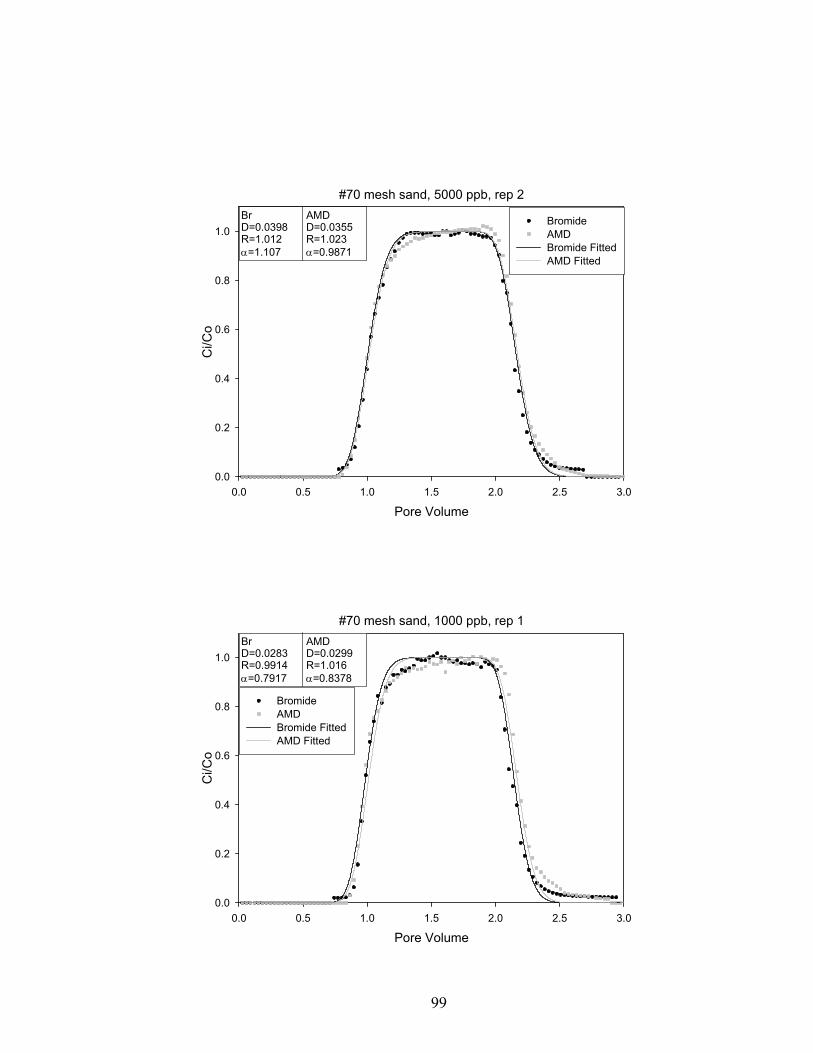
99
#70 mesh sand, 5000 ppb, rep 2
Pore Volume
0.0 0.5 1.0 1.5 2.0 2.5 3.0
Ci/C
o
0.0
0.2
0.4
0.6
0.8
1.0BromideAMDBromide FittedAMD Fitted
BrD=0.0398R=1.012=1.107
AMDD=0.0355R=1.023=0.9871
#70 mesh sand, 1000 ppb, rep 1
Pore Volume
0.0 0.5 1.0 1.5 2.0 2.5 3.0
Ci/C
o
0.0
0.2
0.4
0.6
0.8
1.0
BromideAMDBromide FittedAMD Fitted
BrD=0.0283R=0.9914=0.7917
AMDD=0.0299R=1.016=0.8378

100
#70 mesh sand, 1000 ppb, rep 2
Pore Volume
0.0 0.5 1.0 1.5 2.0 2.5 3.0
Ci/C
o
0.0
0.2
0.4
0.6
0.8
1.0
BromideAMDBromide FittedAMD Fitted
BrD=0.0174R=0.9958=0.4776
AMDD=0.0229R=0.9916=0.6297
#70 mesh sand, 500 ppb, rep 1
Pore Volume
0.0 0.5 1.0 1.5 2.0 2.5 3.0
Ci/C
o
0.0
0.2
0.4
0.6
0.8
1.0
BromideAMDBromide FittedAMD Fitted
BrD=0.0209R=0.9911=0.5804
AMDD=0.0253R=0.9970=0.7016

101
#70 mesh sand, 500 ppb, rep 2
Pore Volume
0.0 0.5 1.0 1.5 2.0 2.5 3.0
Ci/C
o
0.0
0.2
0.4
0.6
0.8
1.0BromideAMDBromide FittedAMD Fitted
BrD=0.0319R=0.9792=0.8.933
AMDD=0.0364R=0.9849=1.020
#70 mesh sand, 100 ppb, rep 1
Pore Volume
0.0 0.5 1.0 1.5 2.0 2.5 3.0
Ci/C
o
0.0
0.2
0.4
0.6
0.8
1.0BromideAMDBromide FittedAMD Fitted
BrD=0.0284R=1.043=0.8237
AMDD=0.0211R=1.032=0.6139

102
#70 mesh sand, 100 ppb, rep 2
Pore Volume
0.0 0.5 1.0 1.5 2.0 2.5 3.0
Ci/C
o
0.0
0.2
0.4
0.6
0.8
1.0BromideAMDBromide FittedAMD Fitted
BrD=0.0278R=1.022=0.8149
AMDD=0.0272R=1.023=0.7959
#70 mesh sand, 50 ppb, rep 1
Pore Volume
0.0 0.5 1.0 1.5 2.0 2.5 3.0
Ci/C
o
0.0
0.2
0.4
0.6
0.8
1.0
BromideAMDBromide FittedAMD Fitted
BrD=0.04597R=1.060=1.370
AMDD=0.0284R=1.028=0.8451

103
#70 mesh sand, 50 ppb, rep 2
Pore Volume
0.0 0.5 1.0 1.5 2.0 2.5 3.0
Ci/C
o
0.0
0.2
0.4
0.6
0.8
1.0BromideAMDBromide FittedAMD Fitted
BrD=0.0355R=1.067=1.742
AMDD=0.0583R=1.021=1.061
C33 sand, 5000 ppb, rep 1
Pore Volume
0.0 0.5 1.0 1.5 2.0 2.5 3.0
Ci/C
o
0.0
0.2
0.4
0.6
0.8
1.0BromideAMDBromide FittedAMD Fitted
BrD=0.0695R=0.981=2.034
AMDD=0.0795R=0.9997=2.326

104
C33 sand, 5000 ppb, rep 2
Pore Volume
0.0 0.5 1.0 1.5 2.0 2.5 3.0
Ci/C
o
0.0
0.2
0.4
0.6
0.8
1.0BromideAMDBromide FittedAMD Fitted
BrD=0.0588R=1.056=1.549
AMDD=0.0825R=1.041=2.171
C33 sand, 1000 ppb, rep 1
Pore Volume
0.0 0.5 1.0 1.5 2.0 2.5 3.0
Ci/C
o
0.0
0.2
0.4
0.6
0.8
1.0BromideAMDBromide FittedAMD Fitted
BrD=0.0548R=1.030=1.565
AMDD=0.0450R=0.9994=1.287

105
C33 sand, 1000 ppb, rep 2
Pore Volume
0.0 0.5 1.0 1.5 2.0 2.5 3.0
Ci/C
o
0.0
0.2
0.4
0.6
0.8
1.0BromideAMDBromide FittedAMD Fitted
BrD=0.0617R=1.040=1.650
AMDD=0.0741R=1.022=1.984
C33 sand, 500 ppb, rep 1
Pore Volume
0.0 0.5 1.0 1.5 2.0 2.5 3.0
Ci/C
o
0.0
0.2
0.4
0.6
0.8
1.0BromideAMDBromide FittedAMD Fitted
BrD=0.0356R=1.036=0.9644
AMDD=0.0574R=1.047=1.555

106
C33 sand, 500 ppb, rep 2
Pore Volume
0.0 0.5 1.0 1.5 2.0 2.5 3.0
Ci/C
o
0.0
0.2
0.4
0.6
0.8
1.0BromideAMDBromide FittedAMD Fitted
BrD=0.0496R=0.9762=1.654
AMDD=0.0603R=0.9992=1.359
C33 sand, 100 ppb, rep 1
Pore Volume
0.0 0.5 1.0 1.5 2.0 2.5 3.0
Ci/C
o
0.0
0.2
0.4
0.6
0.8
1.0BromideAMDBromide FittedAMD Fitted
BrD=0.0540R=0.9940=1.586
AMDD=0.0350R=1.051=1.028

107
C33 sand, 100 ppb, rep 2
Pore Volume
0.0 0.5 1.0 1.5 2.0 2.5 3.0
Ci/C
o
0.0
0.2
0.4
0.6
0.8
1.0BromideAMDBromide FittedAMD Fitted
BrD=0.0312R=0.9604=0.8836
AMDD=0.0371R=0.9996=1.049
C33 sand, 50 ppb, rep 1
Pore Volume
0.0 0.5 1.0 1.5 2.0 2.5 3.0
Ci/C
o
0.0
0.2
0.4
0.6
0.8
1.0BromideAMDBromide FittedAMD Fitted
BrD=0.0301R=1.050=0.8624
AMDD=0.0268R=1.055=0.7673
108
C33 sand, 50 ppb, rep 2
Pore Volume
0.0 0.5 1.0 1.5 2.0 2.5 3.0
Ci/C
o
0.0
0.2
0.4
0.6
0.8
1.0BromideAMDBromide FittedAMD Fitted
BrD=0.0451R=0.9681=1.275
AMDD=0.103R=1.013=2.894
Loam soil, 5000 ppb, rep 1
Pore Volume
0.0 0.5 1.0 1.5 2.0 2.5 3.0
Ci/C
o
0.0
0.2
0.4
0.6
0.8
1.0
BromideAMDBromide FittedAMD Fitted
BrD=0.00435R=0.9244=1.128
AMDD=0.00446R=1.032=1.158

109
Loam soil, 5000 ppb, rep 2
Pore Volume
0.0 0.5 1.0 1.5 2.0 2.5 3.0
Ci/C
o
0.0
0.2
0.4
0.6
0.8
1.0
BromideAMDBromide FittedAMD Fitted
BrD=0.00399R=0.9709=0.9932
AMDD=0.00531R=1.019=1.324
Loam soil, 1000 ppb, rep 1
Pore Volume
0.0 0.5 1.0 1.5 2.0 2.5 3.0
Ci/C
o
0.0
0.2
0.4
0.6
0.8
1.0BromideAMDBromide FittedAMD Fitted
BrD=0.00441R=0.9627=1.149
AMDD=0.00692R=1.072=1.806

110
Loam soil, 1000 ppb, rep 2
Pore Volume
0.0 0.5 1.0 1.5 2.0 2.5 3.0
Ci/C
o
0.0
0.2
0.4
0.6
0.8
1.0BromideAMDBromide FittedAMD Fitted
BrD=0.00614R=0.9588=1.651
AMDD=0.00441R=1.027=1.187
Loam soil, 500 ppb, rep 1
Pore Volume
0.0 0.5 1.0 1.5 2.0 2.5 3.0
Ci/C
o
0.0
0.2
0.4
0.6
0.8
1.0
BromideAMDBromide FittedAMD Fitted
BrD=0.00267R=0.9518=0.6980
AMDD=0.00246R=1.010=0.6433

111
Loam soil, 500 ppb, rep 2
Pore Volume
0.0 0.5 1.0 1.5 2.0 2.5 3.0
Ci/C
o
0.0
0.2
0.4
0.6
0.8
1.0BromideAMDBromide FittedAMD Fitted
BrD=0.00503R=0.9565=1.327
AMDD=0.00343R=0.9893=0.9050
Loam soil, 100 ppb, rep 1
Pore Volume
0.0 0.5 1.0 1.5 2.0 2.5 3.0
Ci/C
o
0.0
0.2
0.4
0.6
0.8
1.0BromideAMDBromide FittedAMD Fitted
BrD=0.00775R=0.9000=2.111
AMDD=0.0103R=1.004=2.807

112
Loam soil, 100 ppb, rep 2
Pore Volume
0.0 0.5 1.0 1.5 2.0 2.5 3.0
Ci/C
o
0.0
0.2
0.4
0.6
0.8
1.0BromideAMDBromide FittedAMD Fitted
BrD=0.00581R=0.9011=1.604
AMDD=0.00491R=1.020=1.356
Loam soil, 50 ppb, rep 1
Pore Volume
0.0 0.5 1.0 1.5 2.0 2.5 3.0
Ci/C
o
0.0
0.2
0.4
0.6
0.8
1.0BromideAMDBromide FittedAMD Fitted
BrD=0.00410R=0.9269=1.126
AMDD=0.00313R=1.021=0.8592

113
Loam soil, 50 ppb, rep 2
Pore Volume
0.0 0.5 1.0 1.5 2.0 2.5 3.0
Ci/C
o
0.0
0.2
0.4
0.6
0.8
1.0BromideAMDBromide FittedAMD Fitted
BrD=0.00436R=0.9435=1.157
AMDD=0.00297R=0.9888=0.7901

114
REFERENCES Ajwa, H., and Trout, T., 2006, Polyacrylamide and water quality effects on infiltration in
Sandy Loam Soils. Soil Science Society of America Journal, v. 70, p. 643-650.
Alef, K., and Nannipieri, P., 1995, Methods in Applied Soil Microbiology and
Biochemistry. London, Academic Press, p. 106, 149.
Bear, F. 1952, Special issue-synthetic soil conditioners. Soil Science, v. 73, p. 419-492.
Blaya, S., Murciano, A., Acebal, P., Carretero, L., Ulibarrena, M., and Firia, A., 2004,
Dirreaction gratings and diffusion coefficient determination of acrylamide and
polyacrylamide in sol-gel glass. Applied Physics Letters, v. 84, n. 23
Brown, L., Bancroft, K., and Rhead, M., 1980, Laboratory studies on the adsorption of
acrylamide monomer by sludge, sediments, clays, peat, and synthetic resins.
Water Research, v. 14, p. 779-781.
Brunauer, S., Emmett, P., and Teller, E., 1938, Adsorption of gases in multimolecular
layers. J. Am. Chem. Soc., v. 60 p. 309-319
Burgisser, C., Cernik, M., Borkovec, M., and Stlcher, H., 1993, Determination of
nonlinear adsorption isotherms from column experiments. An alternative to batch
studies. Environ. Sci. Technol. v. 27 p. 943-948.
Connors, K., 1990, Chemical Kinetics, the study of reaction rates in solution. v. 102(19)
VCH Publishers inc.

115
EPA, 1994a, Consumer factsheet on acrylamide:
http://www.epa.gov/safewater/contaminants/dw_contamfs/acrylami.html.,
updated November 28th, 2006.
EPA, 1994b, Method 8316: Acrylamide, acrylonitrile and acrolein by high performance
liquid chromatography (HPLC).
EPA, 1994c, Acrylic Acid-Stearyl Methacrylate Copolymer; Tolerance Exemption:
http://www.epa.gov/fedrgstr/EPA-PEST/1994/November/Day-02/pr-19.html.,
updated March 29th, 2007.
European Union Risk Assessment Report, 2002, Acrylamide: CAS No: 79-06-1:
http://ecb.jrc.it/DOCUMENTS/Existing-
Chemicals/RISK_ASSESSMENT/REPORT/acrylamidereport011.pdf.
Helalia, A., and Letey, J., 1988, Cationic polymer effects on infiltration rates with a
rainfall simulator. Soil Science Society of America Journal, v. 52, p. 247-250.
Hendrixkx, J., and Dekker, L., 2002, Measurement of solute content using soil extraction:
in Methods of soil analysis: Madison, WI, Soil Science Society of America Inc.,
p. 1255-1261.
Hillel, D., 1998, Environmental Soil Physics. Academic Press. San Diego, CA.
Hirrlinger, B., Stolz, A., and Knackmuss, H., 1996, Purification and properties of an
amidase from Rhodococcus erythopolis MP50 which enantioselectively
hydrolyzed 2-arylpropionamides. J. Baceriol., v. 178, p. 3501-3507
Holliman, P., Clark, J., Williamson, J., and Jones, D., 2005, Model and field studies of
the degradation of cross-linked polyacrylamide gels used during the revegetation
of slate waste. Science of the Total Environment, v. 336, p. 13-24.

116
Hubaux, A., and Vos, G., 1970, Decision and detection limits for linear calibration
curves. Anal. Chem., v. 42, p. 849-855.
Klute, A., and Dirksen, C., 1986, Hydraulic conductivity and diffusivity: Laboratory
methods, in Methods of soil analysis, Part 1. Physical and mineralogical methods,
2nd ed., Klute, A., ed., Agronomy monograph no.9. American Society of
Agronomy. Madison, WI., p. 687-734.
Lahban, S., Moser, D., Arrowood, T., Young, M.H., and Robleto, E. 2007, Fate of
Acrylamide in Soil and Groundwater Systems: Microbial Degradation, Presented
at the American Geophysical Union, Fall Meetings, San Francisco, CA
Lande, S., Bosch, S., and Howard, P., 1979, Degradation and leaching of acrylamide in
soil. Journal of Environmental Quality, v. 8, p. 133-137.
Lentz, R., Shainberg, I., Sojka, R., and Carter, D.L., 1992, Preventing irrigation furrow
erosion with small applications of polymers. Soil Science Society of America
Journal, v. 56, p. 1926-1932.
Lentz, R., and Sojka, R., 1994, Field results using polyacrylamide to manage furrow
erosion and infiltration. Soil Science, v. 158, p. 274-282.
Lentz, R., Sojka, R., and Mackay, B., 2002, Fate and efficacy of polyacrylamide applied
in furrow irrigation: Full-advance and continuous treatments. Journal of
Environmental Quality, v. 31, p. 661-670.
Lentz, R., 2003, Inhibiting water infiltration with polyacrylamide and surfactants:
Applications for irrigated agriculture. Journal of Soil and Water Conservation, v.
58, p. 290-300.
Letey, J., 1996, Effective viscosity of PAM solutions through porous media. IN Sojka,

117
R.E. and R.D. Lentz (eds.) Proceedings: Managing Irrigation-Induced Erosion and
Infiltration with Polyacrylamide May 6, 7, and 8, 1996, College of Southern
Idaho, Twin Falls, ID. University of Idaho Misc. Pub. 101-96, p. 94-96.
Korom S., 2000, An adsorption isotherm for bromide. Water Resources Research, v. 36,
p. 1969–1974.
Maestracci, M., Bui, K., Thiery, A., Arnaud A., and Galzy, P., 1988, The amidases from
a Brevibacterium starins: study and applications. Adv. Biochem. Eng. Biotechnol,
v. 36, p. 67-115.
Malik, M. and Letey J., 1991, Adsorption of polyacrylamide and polysaccharide
polymers on soil materials. Soil Science Society of America Journal, v. 55, p.
380-383.
Malik , M, and Letey, J., 1992, Pore-size-dependant apparent viscosity for organic solutes
in saturated porous media. Soil Science Society of America Journal, v. 56, p.
1032-1035.
Maloszewski, P., Benischke, R., Harum, T., and Zojer, H., 1998, Estimation of solute
transport parameters in a karstic aquifer using artificial tracer experiments: in
Shallow groundwater systems: London, England, Taylor and Francis, p. 188
Mon, J., Flury, M., and Harsh, J., 2006, Sorption of four triarylmethane dyes in a sandy
soil determined by batch and column experiments. Geoderma, v. 113, p. 217-224
Moore, D., and McCabe, G., 1999, Introduction to the Practice of Statistics: 3rd Ed, W.
H. Freeman.

118
Moran, E., 2007, Laboratory studies to examine the impacts of polyacrylamide (PAM) on
Soil Hydraulic Conductivity. MS Thesis, Department of Geological Sciences,
University of Nevada Las Vegas.
Mualem, Y., 1976, A new model predicting the hydraulic conductivity of unsaturated
porous media. Water Resour. Res., v. 12, p. 513-522.
Myers, C., and Nealson, K., 1988, Bacterial manganese reduction and
growth with manganese oxide as the sole electron acceptor. Science, v. 240, p.
1319–1321.
Nadler, A., Malik, M., and Letey, J., 1992, Desortption of polyacrylamide and
polysaccharide polymers from soil materials. Soil Technology, v. 5, p. 91-95.
Nadler, A., Magaritz, M., Leib, L., 1994, PAM application techniques and mobility in
soil. Soil Science, v. 158, n. 4, p. 249-254.
Nagasawa, T., Shimizu H., and Yamada H., 1993, The superiotiry of the third-generation
catalyst, Rhodococcus rhodochrous J1 nitrile hydratase, for industrial production
of acrylamide. Applied microbiology and biotechnoloty, v. 40, n 2.
Nawaz, M., Franklin, W., and Cerniglia C., 1993, Degradation of acrylamide by
immobilized cells of Pseudomonas sp. and Xanthomonas maltophilla.. Can J.
Microbiol., v. 39, p. 207-212.
Nawaz, M., Franklin W., and Cerniglia, C., 1994, Degradation of aliphatic amide mixture
by immobilized and non immobilized cells of Pseudomonas sp. Environ. Sci.
Technol., v. 28, p. 1106-1109.

119
Nawaz, M., Khan, A., Bhattacharayya, D., Siitonen, D., and Cerniglia C., 1996, Physical,
biochemical and immunological characteriszation of a thermostable amidase from
Klecsiella pneumonia NCTR 1. J. Bacteriol., v. 178, p. 2397-2401.
Nawaz, M., Billedeau S., and Cerniglia C., 1998, Influence of selected physical
parameters on the biodegradation of acrylamide by immobilized cells of
Rhodococcus sp.. Biodegradation, v. 9, p. 381-387.
Papiernik, S., and Yates, S., 2002, Processes governing transport of organic solutes: in
Methods of soil analysis: Madison, WI, Soil Science Society of America Inc., p.
1454-1458.
Schaap, M., Leij, F. and van Genuchten, M., 1998, Neural network analysis for
hierarchical prediction of soil water retention and saturated hydraulic
conductivity. Soil Sci. Soc. Am. J., v. 62, p. 847-855.
Shanker, R., Ramakrishna, C., and Seth, P., 1990, Microbial degradation of acrylamide
monomer. Arch Microbiol., v.154, p.192-198.
Šimůnek, J., van Genuchten, M., Sejna, M., Toride, N., and Leij, F., 1999, The
STANMOD computer software for evaluating solute transport in porous media
using analytical solutions of convection-dispersion equation: Versions 1.0 and
2.0.
Šimůnek, J., Šejna, M., and van Genuchten, M., 2006, The HYDRUS software package
for simulating the two-and three-dimensional movement of water, heat, and
multiple solutes in variably-saturated media: Version 1.0.

120
Smith, E., Prues, S., and Oehme, F., 1996, Environmental degradation of
polyacrylamides. 1. Effects of artificial environmental conditions: temperature,
light and pH. Ecotoxicology and Environmental Safety, v. 35, p. 121-135.
Smith, E., Prues, S., and Oehme, F., 1997, Environmental degradation of
polyacrylamides. 2. Effects of environmental (outdoor) exposure. Ecotoxicology
and Environmental Safety, v. 37, p. 76-91.
Sojka, R., and Lentz, R., 1994, Net infiltration and soil erosion effects of a few ppm
polyacrylamide in furrow irrigation water. Proceedings 2nd International
Symposium. 7-11 Feb.,1994, The University of Queensland, Brisbane, Australia.
p. 349-354.
Sojka, R., Lentz, R., Bjorneberg, D., and Aase, J., 1998a, The PAMphlet: A
concise guide for safe and practical use of polyacrylamide (PAM) for irrigation-
induced erosion control and infiltration enhancement. USDA-ARS Northwest
Irrigation & Soils Research Lab., Station Note #02-98.
Sojka, R., Lentz, R., and Westermann, D., 1998b, Water and erosion management with
multiple applications of polyacrylamide in furrow irrigation. Soil Science Society
of America Journal, v. 62, p. 1672-1680.
Sojka, R., Lentz, R., Ross, C., Trout, T., Bjorneberg, D., and Aase, J., 1998c,
Polyacrylamide effects on infiltration in irrigated agriculture. Journal of Soil
Water Conservation, v. 53, p. 325-331.
Spofford, T., and Pfeiffer, K., 1996, Agricultural irrigation polyacrylamide application
standard. In Sojka, R.E. and R.D. Lentz (eds.) Proceedings: Managing Irrigation-
Induced Erosion and Infiltration with Polyacrylamide May 6, 7, and 8, 1996,

121
College of Southern Idaho, Twin Falls, ID. University of Idaho Misc. Pub. 101-
96, p. 49-54.
Susfalk, R., Sada, D., Gates, T., Epstein, B., Martin, C., Smith, D., Schmidt, M., Young,
M., and Rosamond, C., 2007, Application of Granular, Linear anionic
Polyacrylamide (PAM) to Water Delivery Canals for Water Conservation. DRI
Publication, In preparation.
van Genuchten, M., 1980, A closed-form equation for predicting the hydraulic
conductivity of unsaturated soils. Soil Sci. Soc. Am. J., v. 44, p. 892-898
van Genuchten, M., Davidson, J., and Wierenga, P., 1974, Evaluation of kinetic and
equilibrium equations for prediction of pesticide movement through porous-
media. Soil Sci. Soc. Am. J., v. 38, p. 29-35
Vers, L., 1999, Determination of acrylamide monomer in polyacrylamide degradation
studies by high-performance liquid chromatography. Journal of Chromatographic
Science, v. 37, p. 486-94.
World Health Organization, 1997, Environmental Health Criteria, No 191: acrylic acid
Wolin, E., Wolin, M., and Wolfe, R., 1963, Formation of methane by bacterial extracts. J.
Biol. Chem., v. 121, p. 184−191.
Woodrow, J., and Miller, G., 2007, UV degradation of LA-PAM and AMD in, Results of
laboratory experiments in support of PAM-related research, M.H. Young, editor.
DRI publication no. 41237.
Young, M.H. J.J. Tappen, G.C. Miller, S. Carroll, R.B. Susfalk, 2007, Initial Risk
Characterization: Using Linear Anionic Polyacrylamide (LA-PAM) to Reduce

122
Water Seepage from Unlined Water Delivery Canal Systems. DRI Publication
No. 41226.
123
VITA
Graduate College University of Nevada, Las Vegas
Todd J. Arrowood
Home Address: 8044 Secretariat lane Las Vegas, NV 89123
Degrees:
Bachelor of Science, Geoscience, 2005 University of Nevada, Las Vegas
Publications: Arrowood, T., and Young, M.H. 2007. AMD sorption in soil/water systems in, Results of
Laboratory Experiments in Support of PAM-Related Research, M.H. Young, Editor. DRI Publication No. 41237.
Presentations: Arrowood, T., Young, M.H., 2007, Determining the Transport of the Acrylamide
Monomer (AMD) in Soil and Groundwater Systems, UNLV Geosymposium Arrowood, T., Young, M.H., Yu, Z. 2006, Determining the Transport of the Acrylamide
Monomer (AMD) in Soil and Groundwater Systems, UNLV Geosymposium Arrowood, T., Young, M.H., Yu, Z., Lahban, S., and Moser, D. 2007, Fate and Transport
of Acrylamide in soil and groundwater systems: Sorption, Retardation and Numerical Simulations, Presented at the American Geophysical Union, Fall Meetings, San Francisco, CA
Lahban, S., Moser, D., Arrowood, T., Young, M.H., and Robleto, E. 2007, Fate of Acrylamide in Soil and Groundwater Systems: Microbial Degradation, Presented at the American Geophysical Union, Fall Meetings, San Francisco, CA
Thesis Title: Determining the Fate and Transport of the Acrylamide Monomer (AMD) in Soil and Groundwater Systems.
Thesis Examination Committee:
Chairperson, Dr. Zhongbo Yu, Ph.D. Co-Chairperson, Dr. Michael Young, Ph.D. Committee Member, Dr. Dave Kreamer, Ph.D. Graduate Faculty Representative, Dr. Thomas Piechota, Ph.D.