DETERMINATION OF THE MOST SUITABLE OIL PIPELINE

ROUTE USING GIS LEAST COST PATH ANALYSIS.

Shahin Huseynli

Case Study: Keystone XL, Nebraska State - USA

DETERMINATION OF THE MOST SUITABLE OIL

PIPELINE ROUTE USING GIS LEAST COST PATH

ANALYSIS.

Case Study: Keystone XL, Nebraska State - USA

Dissertation supervised by

Dr.Marco Painho

Dr.Sven Casteleyn

Dr.Rauf Amanov

February 2015

ACKNOWLADGEMENTS

I would like to express my gratitude to all who was responsible on this

educational program and especially Dr.Prof.Marco Painho. I would like to give

special thanks to my co-supervisor Dr. Sven Casteleyn and Dr. Rauf Amanov

because of their help on this thesis.

Also I am particularly grateful to my family for their support in all cases

DETERMINATION OF THE MOST SUITABLE OIL

PIPELINE ROUTE USING GIS LEAST COST PATH

ANALYSIS.

Case Study: Keystone XL, Nebraska State - USA

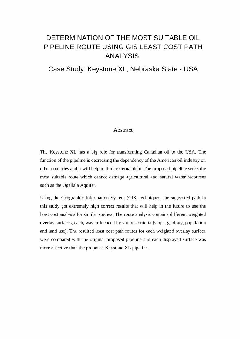
Abstract

The Keystone XL has a big role for transforming Canadian oil to the USA. The

function of the pipeline is decreasing the dependency of the American oil industry on

other countries and it will help to limit external debt. The proposed pipeline seeks the

most suitable route which cannot damage agricultural and natural water recourses

such as the Ogallala Aquifer.

Using the Geographic Information System (GIS) techniques, the suggested path in

this study got extremely high correct results that will help in the future to use the

least cost analysis for similar studies. The route analysis contains different weighted

overlay surfaces, each, was influenced by various criteria (slope, geology, population

and land use). The resulted least cost path routes for each weighted overlay surface

were compared with the original proposed pipeline and each displayed surface was

more effective than the proposed Keystone XL pipeline.

Keywords

Keystone XL

Pipeline

The Ogallala Aquifer

GIS

Least Cost Analysis

Nebraska

Oil

Acronyms

GIS – Geographical Information System

KXL – Keystone eXport Limited

LCP – Least Cost Path

SCP – Straight Line Path

CSD – Conversation and Survey division

US - United States

DEM – Digital Elevation Model

USGS – United States Geological Survey

SRTM – Shuttle Radar Topography Mission

GPS – Global Positioning System

ESRI – Environmental Systems Research Institute

INDEX OF CONTENT

ACKNOWLADGEMENT………………………………………………………...…ii

ABSTRACT ...............................................................................................................iii

KEYWORDS………...................................................................................................iv

ACRONYMS...............................................................................................................v

INDEX OF TABLES…………………………………………………………..…… vi

INDEX OF FIGURES …………………......……………………………………… vii

1.INTRODUCTION………………………………………………………………...1

1.1 Overview..…...………………………………………………………………..1

1.2 Keystone XL………………………………………………………………….2

1.3 Geo-political and Economic issues…………………………………………...3

1.4 Least Cost Analyses….….……………………………………………………5

1.5 Objectives………………………………………………………………….…6

2 .LITERATURE REVIEW ……………………………………................................7

3. STUDY AREA ……………………………………………………………….…11

4. METHODOLGY AND DATA …………………………………………….…….14

4.1 Methodology………………………………………………………….…….14

4.2 Data Sets……………………………………………………………….…...16

4.3 Accumulative Cost Surface………………………………………………...21

4.4 Least Cost Routing Tool…………………………………………….….….23

5. RESULT………………………………………………………………….……...24

5.1 Equal Weighted Overlay ………………………………………………….24

5.2 Weighted Overlay………………………………………………………....27

5.3 The Ogallala Aquifer and Proposed Keystone XL………………………..34

6. DISCUSSION…………………………………….…………………………..…40

7. CONCLUSION…………………………………………………………………44

8 .BIBLIOGRAPHICAL REFERENCES…............................................................45

ANNEX A…………………………………………………………………………48

ANNEX B………………………………………………………………………….52

INDEX OF THE TABLES

Table 1. Least Cost route lengths and Straight Line route length, which based on

Equal Weighted Cost surface………………………………………………………..26

Table 2. All three Weighted Overlays with specific weighted percentage for each

criterion……………………………………………………………………………...28

Table 3. Least Cost route lengths and Straight Line routes length, which based on

Weighted Overlay 1, Weighted Overlay 2 and Weighted Overlay 3 cost surfaces....33

Table 4. The percentages and length of the routes, which passed through the Ogallala

Aquifer………………………………………………………………………………37

TABLES IN ANNEX 1

Table 1. Data processing for “Environmental Criterion”…………………………...48

Table 2. Data processing for “Geology” Criterion…………………………………49

Table 3. Data processing for “Land Use” criterion…………………………………50

Table 4. Data processing for “Slope” criterion……………………………………...51

INDEX OF THE FIGURES

Figure1. Keystone Pipeline Route. (TransCanada Corporation 2012)……………….3

Figure 2. Top Oil Exports to the United States .1973-2013 (U.S. Energy Information

Agency)………………………………………………………………………….……5

Figure 3. Ogallala Aquifer. (Map applies to

1997)……………………………….….12

Figure 4. The first Keystone XL proposed pipeline. (Keystone-

XL.com)…………..13

Figure 5. Data proccesing and factor rasters shown as a criterion

datasets…………...15

Figure 6. Geological map data for Geology criterion of Nebraska

(USGS)…………16

Figure 7. Elevation data for Slope criterion of Nebraska (NASA JPL)……………..18

Figure 8. Land Use data for land use critertion of Nebraska (University of

Nebraska)……………………………………………………………………………19

Figure 9. Envirnonmental data map for environmental criterion(Census)………….20

Figure 10. Equal Weight cost surface that was formed for the study area………….24

Figure 11. Equal Weighted LCP and straight-line route, which achieved for cost

surface Equal Weights overlay………………………………………….………......25

Figure 12. Least Cost Route and Straight Line path for Weighted Overlay Surface

1…………………………………………………………….……….…..…………..30

Figure 13. Least Cost Route and Straight Line path for Weighted Overlay Surface

2……………………………………………………………………………………...31

Figure 14. Least Cost Route and Straight Line path for Weighted Overlay Surface

3…………………………………………………………………………….………..32

Figure 15. The proposed Keystone XL from Trans Canadian Corporation and all

least cost path routes displayed on the slope surface…………….………………….35

Figure 16. The Least Cost Path route, which is related to the Weighted Overlay 3 and

shown with the Ogallala Aquifer geological map…………………………………...38

FIGURES IN ANNEX B.

Figure 1. Displays the procedure of least cost path………………………………....52

Figure 2. “Weighted Overlay 2 Least Cost Path” and not understandable part of the

route…………………………………………………………………………………53

1

1. Introduction

1.1 Overview

Nowadays natural resources are one of the key factors of developing the economic

situation of any country. U.S and some other countries in North America are more

famous for their natural resources more than other regions in the world. Fertile soils,

plentiful freshwater, natural gas and oil, mineral deposits and forestry are the key

elements of natural resources in North America which directly have influenced their

economy.

Pipelines are the most efficient, cost effective and environment friendly means of

fluid transport and reduce the highway congestion, pollution and spill (Dubey, 2005).

Careful planning of the pipeline route can save cost, time and operating expenses to

ensure longer operational life and help in preventing environmental fallouts. Proper

planning and management are considered essential means of guiding and

accelerating the development of an industry. It can mobilize and utilize the available

resources in the best interest of the company and eliminate business fluctuation

(Nasir and Hyder, 2001). Routing a pipeline is an important task thus proper

planning is essential in-order to maximize the benefits derivable from the use of

pipelines. With the scientific planning of a route, cost, time, and operating expenses

can be saved, ensuring longer operational life and minimizing environmental

fallouts.

Every day in our life technology is developing and it helps to develop some

particular sciences which concentrated in different educational fields. The latest

technology and recent researches shows that GIS is the best tool (or science) for

environmental planning and regulatory conformity. Geographical Information

Science in itself has a big role in various geographical areas including pipeline

routing. Pipelines are one of the most expensive and very sensitive transportations

2

type that according to their capability, they can manage really big projects. But in the

other hand, even small mistakes can create huge problems. Hence, GIS in this more

suitable way to protect areas from hazards and also solve problems such as oil spills,

gas leak and etc.

GIS in different trends can help to understand specific fields of the pipeline and also

it can help to routing process. With influence of GIS it was already possible to create

route corridors for different transportation types. Special algorithm for routing first

time done by Dutch scientist Edser Djikstra in 1956 and for more detailed

information written in literature review part of the thesis. Later famous American

geographer Michael Goodchild with using the Djikstra Algorithm have founded

evaluation of lattice solution to the corridor locations in 1977. With the same

methodology M. Goodchild gave new breath to the modern technology and science.

But thesis more concentrated on the route analysing and that is why, study

concentrated on Djikstra Algorithm.

1.2 Least Cost Analyses.

The study is converged on finding the least cost routing strategy applying GIS

analysis to the geographic area where Keystone XL will pass through Nebraska

State. The routing model defines the most economical and environmentally safe

route through the given study area. The study is highly concerned about avoiding

geological, social and environmental hazards. This study would allow working with

large-scale projects in the future and it will help also to find less hazardous

methodology for routing the pipeline.

The most sensitive problems in pipeline routing are geological factors, land use

information, slope and some another criteria which could help researchers to

determine the least cost routing. With using ArcGIS Cost Path tool, it would be

easier to understand the problems in the study area and also to determine the least

cost routing. All criteria were collected into the ArcGIS geodatabase and data file

digitized and rasterized for specific hazard weights

3

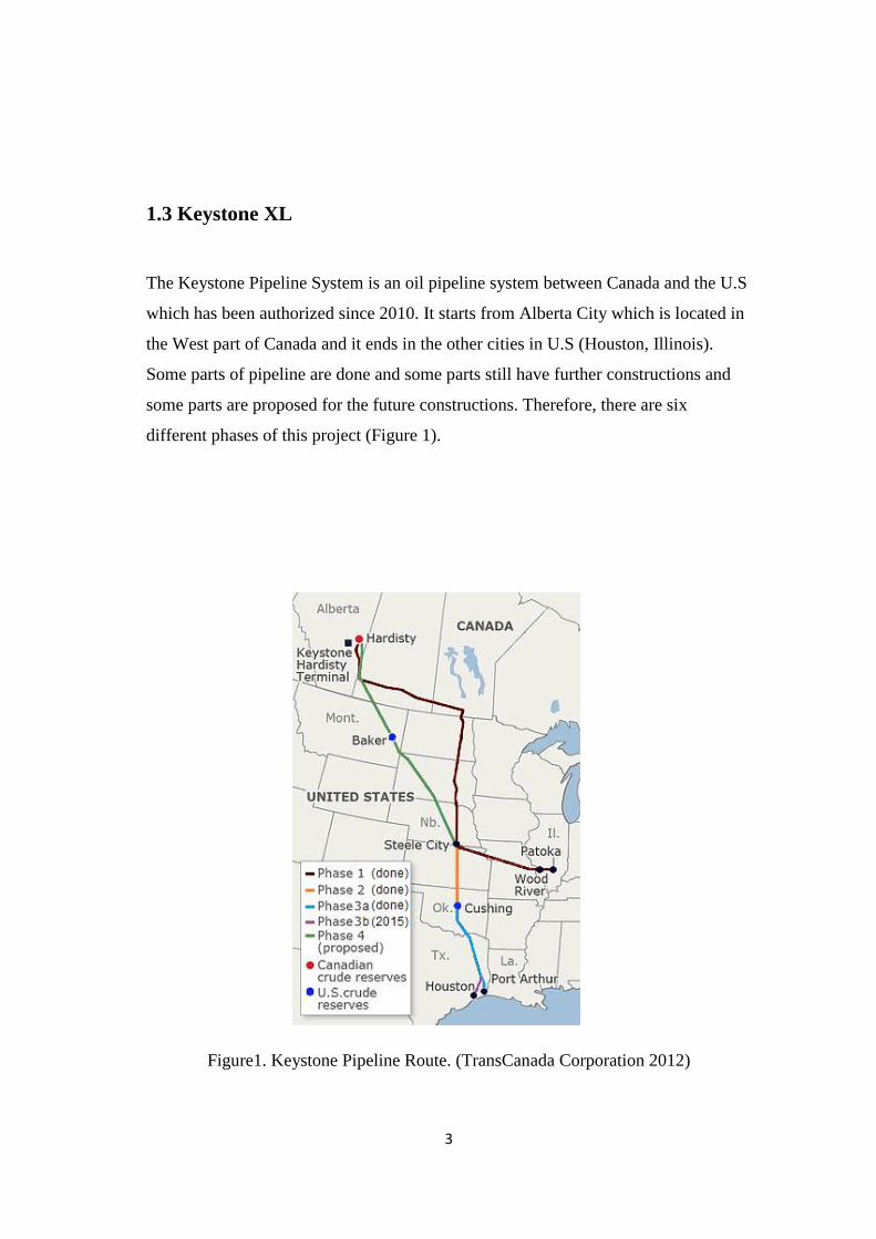
1.3 Keystone XL

The Keystone Pipeline System is an oil pipeline system between Canada and the U.S

which has been authorized since 2010. It starts from Alberta City which is located in

the West part of Canada and it ends in the other cities in U.S (Houston, Illinois).

Some parts of pipeline are done and some parts still have further constructions and

some parts are proposed for the future constructions. Therefore, there are six

different phases of this project (Figure 1).

Figure1. Keystone Pipeline Route. (TransCanada Corporation 2012)

4

Figure 1 displayed parts of the pipeline which have been already done as well as the

proposed parts. The study focuses on Phase 4 which also called Keystone XL

(Keystone eXport Limited), with a special interest in the second edition of pipeline

extension proposed in 2008 by National Energy Board of Canada. On March 11,

2010 the Canadian National Energy Board approved the project.

Keystone XL starts from Hardesty City in Canada and it ends in Steele City in

Nebraska State. The length of the proposed pipeline is 18.974 km (1.179 mile), but

there is a big issue about environmental hazards. In 2011 a scientist from NASA

James Hansen, mentioned that Keystone XL can make a big global warming with

one small mistake, such as, oil spill. According to the State Department’s review, the

830,000 barrels are going to be transformed through the Keystone pipeline daily and

it means that it would add extra amount of carbon dioxide which approximately

ranges from 1.3 to 27.4 million metric tons to the atmosphere. These numbers are

only recorded in 2013, so it means that this hazard can be more serious than any

expectations. Keystone XL is the most suitable choice for U.S government to

transport oil from neighbor country. It tried to find more options for shipping

Canada’s oil to US but it did not work (Brad Plumer 2015).

First of all, they tried to understand if it was possible to make shipping with trains

but it would cost two times more expensive than the current budget (approximately 8

billion dollars) of Keystone and it would be more dangerous for the environment

compare with Keystone XL. In this way, maximum shipping capabilities can hardly

reach 165.000 barrels per day. Moreover, other scientists had an idea about shipping

with big boats but it was not good idea because they even did not pay attention to

what had happened in “Gulf of Mexico” in 2010.

5

1.4 Geo-political and Economic issues.

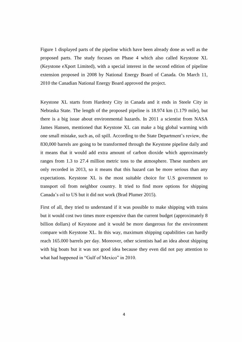
U.S House of Representatives, Committee on Energy and Commerce proponents

made a lot of debates about Keystone XL. In their opinion, Keystone XL would

allow U.S to increase energy security in the region and reduce its dependence on

foreign oil. U.S is on the top of oil importing country, it imports oil almost from all

continents (Figure 2).

Figure 2. Top Oil Exports to the United States .1973-2013 (U.S. Energy Information

Agency).

American authorities have another idea about a project that KXL can help to increase

the price of the oil in Midwestern United States. It can help to partially solve their

dept. The Keystone XL would also create approximately 42,000 job opportunities

during the next few years and 3900 temporary constructions (The State Department,

2015). The project would push approximately 3.4 billion dollars to the economy

which represents 0.02% of US GDP (Brad Plumer 2015, www.vox.com).

There is another key issue that some part of thesis concentrated aquifer where is the

one of the biggest groundwater basin located in central U.S that proposed Keystone

XL passing through the this area. The idea of the study to create suitable route which

6

is not passing through the area. The Ogallala Aquifer is the one of the hugest aquifer

which underlies approximately 450.000𝑘𝑚2. The Aquifer is part of the high plains

aquifer system which is the principal geologic unit covering 80% of the high plains.

It has really big role in agricultural and environmental trends. Therefore, 70% of the

aquifer protecting by U.S government and other 30% using as a water resource for

the agriculture and for environmental issues.

.

1.5 Objectives

The objectives of the study is about to understanding the suitable route for the

Nebraska State. Using the least cost path analyses it will be possible to find out what

is the beneficial route or least hazardous route which cannot damage region

environmentally, agriculturally and understand which route is suitable to prevent the

area from expecting natural hazards from the study area. Nebraska State more

famous with their agricultural issues and it is because of the agricultural zones

located on high plains which has direct connection with the Ogallala Aquifer. Hence,

proposed Keystone XL from TransCanada Corporation rejected by U.S government

in 2014 after long period research. This pipeline rejected because of the most part of

the pipeline was passing through aquifer area and also it will be second issue for the

thesis, how to least cost path analyses will behave for following groundwater area. It

was not possible to get exact data with more information about proposed pipeline and

that is why, during the project there will be Euclidean path route which will help to

understand effectiveness of each routes. Euclidean path chosen as prototype of

proposed Keystone XL and this kind of path works only between two points (source

and destination). In the thesis source point take into account Key Paha city which

Nebraska part of the pipeline starting from there and destination chosen as Steele

City in the South of the Nebraska State.

7

2. Literature Review

Large-scale linear projects, such as natural gas and oil pipelines, are planned and

designed about a short route to limit the costs and materials of production. The most

effective process to determine this route is through the use of GIS and a least-cost

routing model (Aissi, Chakhar, and Mousseau 2012; Rees 2004; Feldman et al.

1995).The latest GIS techniques helps us for large amounts of cost-analysis data to

be collected, stored and analyzed and improve the route accuracy for large-scale

projects (Luettinger and Clark 2005). During the research of some studies as an

example in previous studies, the methodology formulated to create least cost model

for specific and various criteria evaluations and corporate simple criteria into one of

least cost model. The complications of least cost models have limited with different

categories of criteria and also they have been examined during studies. Most of

criteria have been examined with physical characteristics of geographic area during

the straightforward point of view to weighting the alteration of special factors.

(Chakhar, and Mousseau 2012). In general there are not enough studies which have

included impacts when to find the unique route selections of a pipeline and in

included these criteria inside of model. Only one, (Lovett 1997) and one theses about

least cost path analyses to route risky waste through study area and specific paths and

both of this research provided a risk assessment due to biological hazards as an

example population and environmental risk. (Lovett, Parfitt, and Brainard 1997;

Kelly 2014)

Special ways to how to develop a process to determine the shortest, the lowest

hazardous and least costly routes have had academic analyzing different techniques

for many years. One of the first academic Edsger Dijkstra has founded way to solve

problem. He developed an algorithm to determine the shortest path between two

points connected in a network (Dijkstra 1959). This algorithm is one of the key

elements that is included in many least cost routing models. In conjunction with a

cost accumulated surface the algorithm is able to choose the least cost route across a

8

given area. This kind of analyzes related on the neighborhood of cells around the

proposed starting point and moves external from starting point to finally encompass

the given study area. There are a lot of types of model that the algorithm can create

cost accumulated surface with different patterns offering a different approach to

solve the problem (Iqbal, Sattar, and Nawaz 2006; Luettinger and Clark 2005). The

algorithm of Dijkstra is one of the commonly used tools to determine the least cost

route through a surface and one of the simplest methods. That is already one fact that

only with that algorithm can analyze various criteria and complied together into a

cost accumulated surface and need only analyze knot across the surface. Only one

restriction; however to using this type of algorithm is that it is computationally

demanding and produces large amounts of data (Saha 2005).

To improve on this computationally demanding process has been used more and

more companies began to develop new GIS packages to restrict computation time

and accelerate results. The Environmental Systems Research Institute (ESRI) made a

tool which called “Pathdistance” and it uses a smaller scale neighborhood analysis in

order to try and control the effects of the model and make the path more realistic

(Saha 2005). In effect to use of this smaller scale would help to make the compiled

path less irregular and sleeker. This is a key when planning pipeline route due to the

fact that a pipeline is connected together much more rigidly than a road. That is why

“Pathdistance” tool became more prominent in studies due to their accessibility and

this option to create much smoother designs. Downside of studies was that the

limitation of the neighborhood. Analysis meant they could not accurately predict

points in mountainous areas. (Saha 2005). The rapidly changing topography would

be generalized too much in the cost accumulated surface for an accurate assessment

of the route to be determined. Recent years ESRI developed more complex cost path

extensions and made them together inside of the ArcGIS products. One of these

extensions such as Cost Path tool has a significant rule about routing pipeline or to

determine such more suitable routing place. This tools allows for the creation of both

a Cost Distance surface and a Backlink surface that are then used alongside the main

Cost surface to determine a more accurate and precise Cost Path from a source point

9

to a destination point, all of these methods calculate the cost that path acquires across

the surface (Collischonn and Pilar 2000; Rees 2004).

Current case studies have been performed to determine the least cost routes of major

pipelines are mainly founded by major operators in the study. In the study

researchers utilize both remote sensing and GIS data develop necessary criteria for

analysis, For example: Bechtel Corporation in its analysis to develop a route a

proposed pipeline in the Caspian Sea region provided one such case study. The

researchers made a factors from the terrain, land use, geology and etc. through the

use of geospatial data sets (Saha 2005; Feldman 1995).Using the remotely sensed

data allows for areas all over the globe to be examined and evaluated without the

physically travelling to the specific locations. The cost associated with the

construction in each specific criterion was determined from previous study that was

not published by Bechtel, permitting the researchers to obtain a greater accuracy on

the real world costs. There were some factors that costs were also environmental and

future liability costs should the pipeline to faults, river crossings (Feldman 1995).

Feldman is one of the first studies actively and effectively integrate these types of

criteria into the least cost routing model during the availability of remotely sensed

and previously researched cost data. Due to researching time the use of ArcGIS

software, the route that was proposed was 9 km longer than the straight line path but

14% less costly to construct (Feldman 1995). This kind of research helped to us

determine the study area for less costly amount and with the available works which

could help to researchers to examined the studies through the use of geospatial data.

There was some another methods to determine the least costly routes through study

area and it called “View-shed analysis” (Lee and Stucky 1998). The general

methodology almost the same with thesis’s methodology that is discussed previous

chapters in this thesis is used to create a cost accumulated surface and a least cost

algorithm. In using the view-shed analysis by Lee and Stucky 1998 a digital

elevation model (DEM) selected in 4 types of paths in study area. But this analysis

more useful for environmental planning and civil engineering for testing the pipeline

construction, the analysis returns to results (Lee and Stucky 1998). And also in the

10

methodology do not need some factors which have a big role in routing pipeline. For

analysis there were no factors such as geology, terrain or land use etc. (Saha 2005;

Lee and Stucky 1998). Therefore for pipeline routing and the focus of this thesis,

view- shed did not use into the methodology.

There were some studies which have been done more currently focused on the costs

of crossing water bodies and the built environmental (roads, bridge, etc) and on the

slopes (Iqbal, Sattar and Nawaz 2006). The areas analyzed by researcher Iqbal in

2006, was more focused on the mountainous region of the North part of India, where

the changes of grades of the terrain in short distances played a key role for

determining where pipeline could be located. The criteria that were analyzed were

first reclassified through a Spatial Decision Support System (SDSS) to make the

system more result oriented and simpler to process (Iqbal, Sattar and Nawaz 2006).

As a result of this least cost route was 1 km longer than existing pipeline in area but

it was 29% less costly compare with existing pipeline. The use of the least cost

model accurately displayed a more economical route and can be integrated into many

other fields such as the planning water pipelines which also require more economical

routing plans (Iqbal, Sattar and Nawaz 2006).

Other linear features which were similar to natural gas and oil pipelines that have

used least cost routing models to more accurately plan the economic routes are roads

and canals. Because, usually those kinds of works which related with water bodies

and sources costs to more expensive and need more works to be sure with done as

long as in the possible time period. And for understanding routes, especially in

canals, features impacts of topography more important and influences the cost

accumulated surface by making the weight values direction. With specific

requirement the algorithms used to process the cost accumulated surface must be

adapted to accommodate restriction (Collischon and Pilar 2000).

11

3. Study Area

The proposed Keystone XL pipeline passes through three states in US (Montana,

South Dakota and Nebraska). It is more likely to cause some hazardous problems in

Nebraska. That is why, Nebraska was considered as the study area of the thesis. Until

the beginning of the Keystone XL project, there were not pipelines which could

naturally or economically affect the region. The total study area is 200,520 square

kilometers and the economic income mostly depends on wind power and solar

power. The capital city of the state is Lincoln and the estimated population was

1.800.000 capita in 2014. Keystone XL would be the first and largest pipeline which

passes through eastern part of Nebraska. After first proposed pipeline, there were

wide oppositions inside Nebraska regarding declining the project because of the

expected pollution and global warming. The proposed Keystone XL was passing

through the middle of the Ogallala Aquifer and could make dangerous hazard

problem to the region (Figure 3).

12

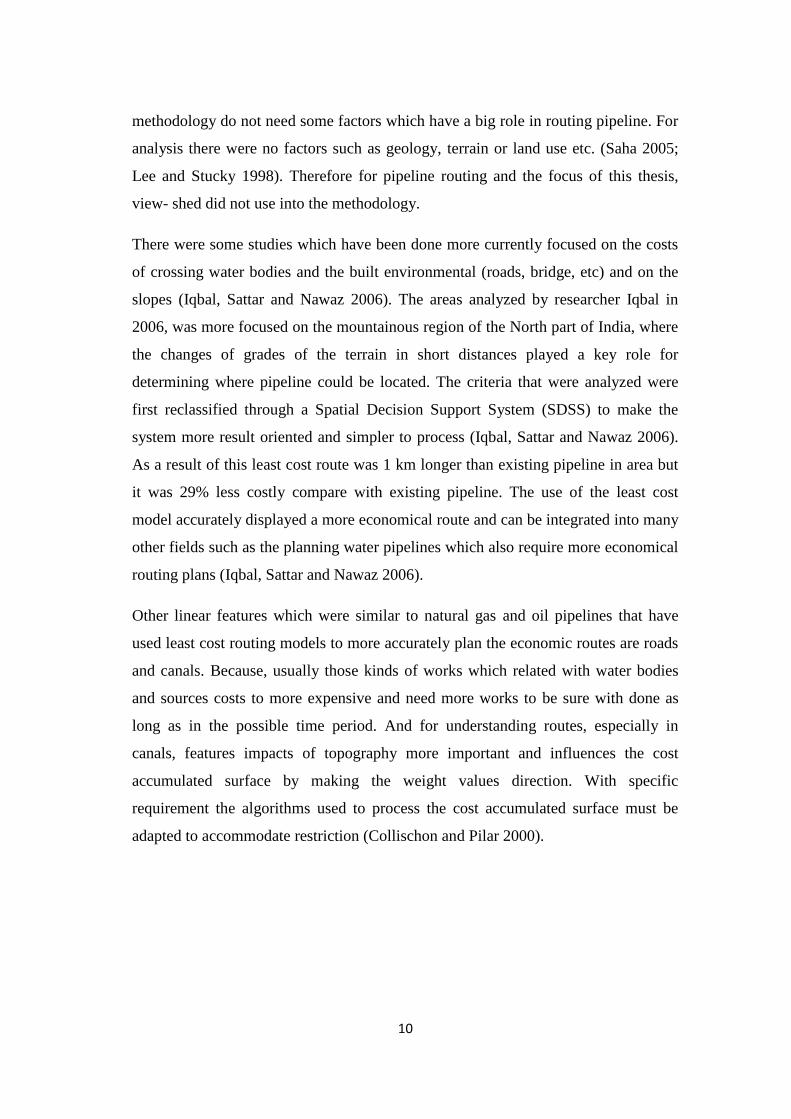
Figure 3. Ogallala Aquifer. (Map applies to 1997)

Another key element of study area is located in the Ogallala Aquifer (Figure 3). This

aquifer is one of the biggest water bodies in the world and also it has a significant

influence on importing water to Nebraska and other neighbor states.

Initial steps about Keystone XL were proposed to pass through the East part of

aquifer. But this issue could be more dangerous for following study area. Dr Jim

Goeke, a research hydrologist and professor said that the Ogallala Aquifer providing

more million’s people with quality water and it is necessary to try find more suitable

routing way for Keystone XL. Small incident can make big problems and even there

were some parts of aquifer deepest parts changes between 50 and 300 feet (Figure 4)

13

and also this shows us first proposed pipeline was not good enough for routing

process. Keystone XL’s path is east of more than 80% of the Ogallala Aquifer.

Impact modeling conducted by the State Department and the Nebraska Department

of Environmental Quality has shown that in the very unlikely event of an incident,

impacts would be localized to as little as tens of feet (Keystone-xl.com).

Figure 4. The first Keystone XL proposed pipeline. (Keystone-XL.com)

14

4. Methodology and Data

4.1 Methodology

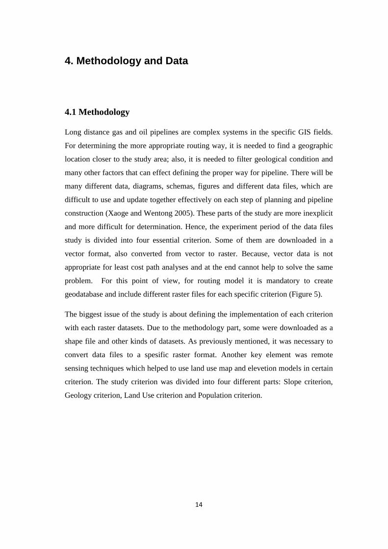
Long distance gas and oil pipelines are complex systems in the specific GIS fields.

For determining the more appropriate routing way, it is needed to find a geographic

location closer to the study area; also, it is needed to filter geological condition and

many other factors that can effect defining the proper way for pipeline. There will be

many different data, diagrams, schemas, figures and different data files, which are

difficult to use and update together effectively on each step of planning and pipeline

construction (Xaoge and Wentong 2005). These parts of the study are more inexplicit

and more difficult for determination. Hence, the experiment period of the data files

study is divided into four essential criterion. Some of them are downloaded in a

vector format, also converted from vector to raster. Because, vector data is not

appropriate for least cost path analyses and at the end cannot help to solve the same

problem. For this point of view, for routing model it is mandatory to create

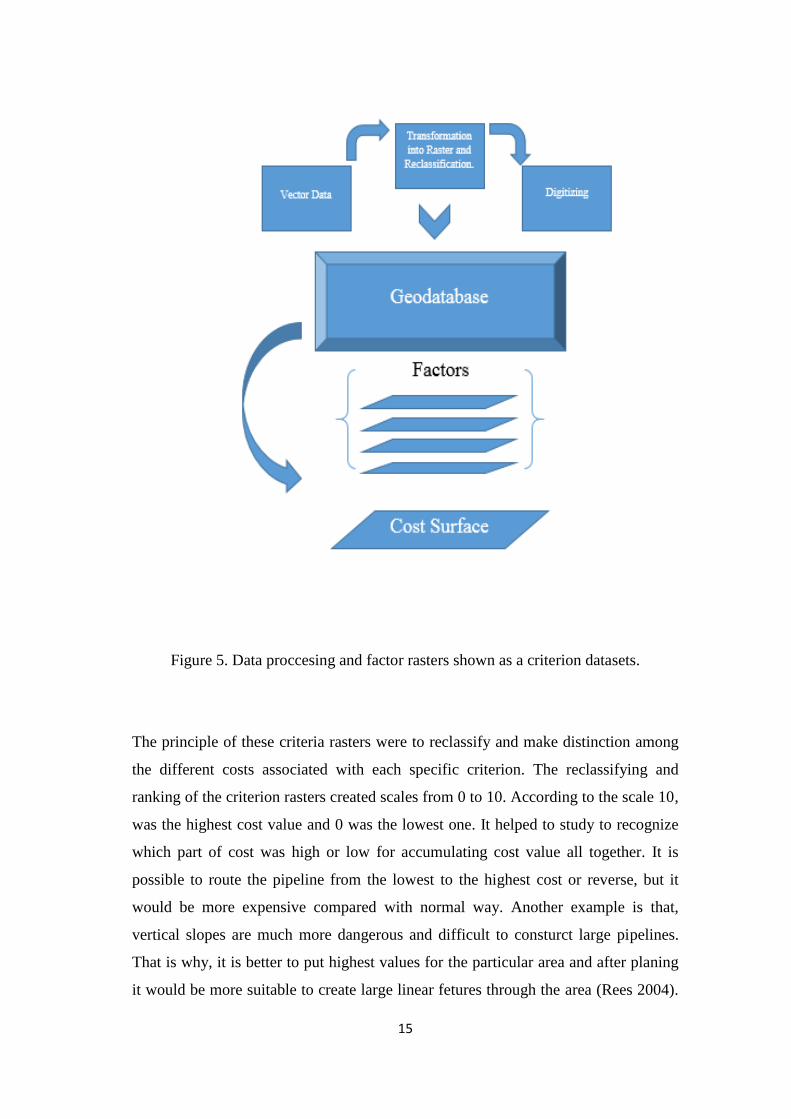
geodatabase and include different raster files for each specific criterion (Figure 5).

The biggest issue of the study is about defining the implementation of each criterion

with each raster datasets. Due to the methodology part, some were downloaded as a

shape file and other kinds of datasets. As previously mentioned, it was necessary to

convert data files to a spesific raster format. Another key element was remote

sensing techniques which helped to use land use map and elevetion models in certain

criterion. The study criterion was divided into four different parts: Slope criterion,

Geology criterion, Land Use criterion and Population criterion.

15

Figure 5. Data proccesing and factor rasters shown as a criterion datasets.

The principle of these criteria rasters were to reclassify and make distinction among

the different costs associated with each specific criterion. The reclassifying and

ranking of the criterion rasters created scales from 0 to 10. According to the scale 10,

was the highest cost value and 0 was the lowest one. It helped to study to recognize

which part of cost was high or low for accumulating cost value all together. It is

possible to route the pipeline from the lowest to the highest cost or reverse, but it

would be more expensive compared with normal way. Another example is that,

vertical slopes are much more dangerous and difficult to consturct large pipelines.

That is why, it is better to put highest values for the particular area and after planing

it would be more suitable to create large linear fetures through the area (Rees 2004).

16

In case of the study determinations of the certain rankings, the same techniques were

used (Feldman 1995).

The created routes were compared to one another and also a straight-line path

through the study area to determine the cost benefits of the analysis and to make sure

that the routes were realistic. Multiple routes were created with differing weights for

each criterion in order to see what geographic locations are most affected by each

specific factor. The unit calculations that were derived from the tool were also

compared to one another to identify if the weighting system increased the costs

associated with the pipeline or decreased them.

4.2 Data Sets

For the least cost path analyses, it is needed more detailed and accurate datasets,

especially for geological criterion. The reason is that, implementation of less

hazardous ways need more comprehensibile datasets for area. Geological criterion in

thesis was downloaded with full detailed information, while some parts which were

not good enough for routing were ereased from ArcGIS and digitized for the study

area. The data was downloaded as a vector file and with the help of ArcGIS, was

converted from the vector to the raster file in order to display the continous surface.

At the same time, the geological raster that was created to display the highest cost

values contain geologically young and the lowest contain geologically old, due to

their higher stability or load bearing proporties (Paige and Green 2011).

17

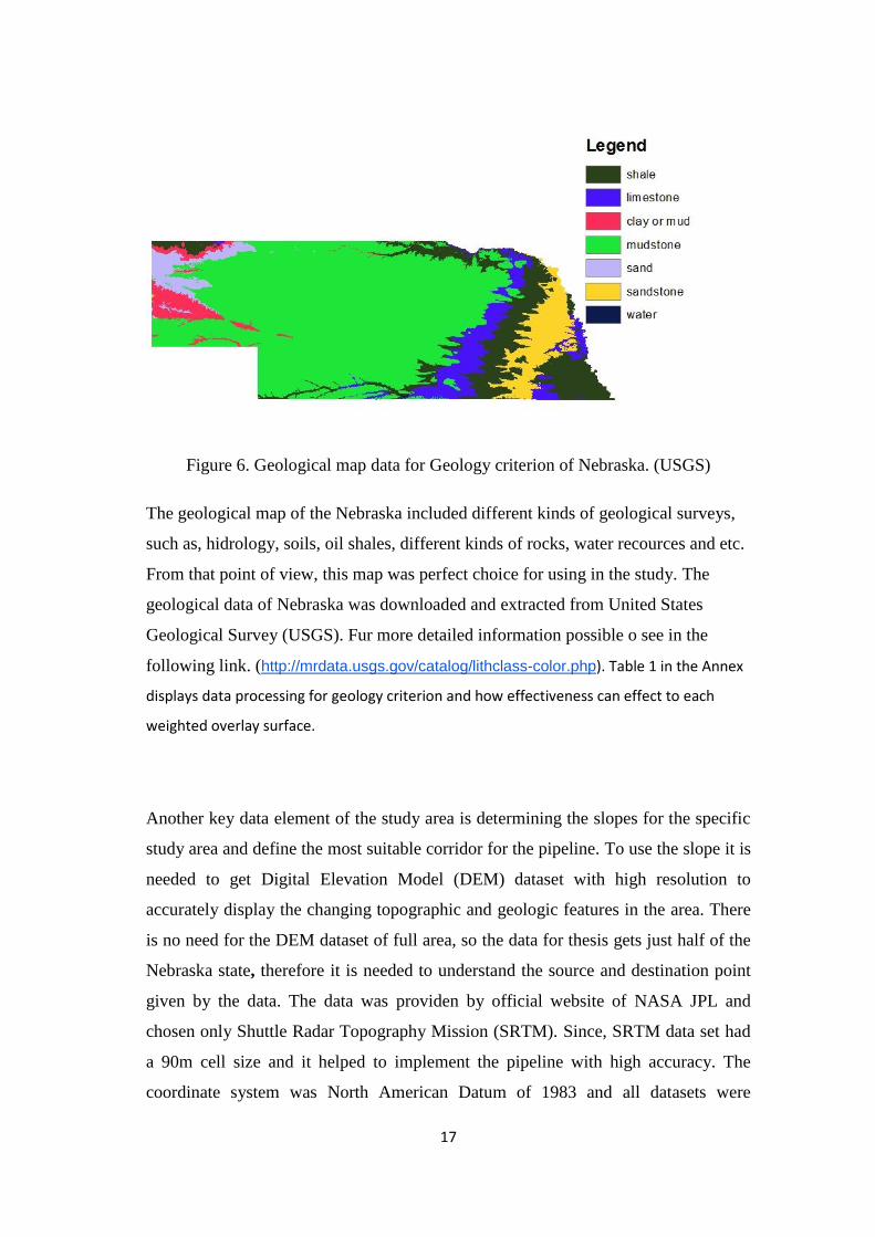
Figure 6. Geological map data for Geology criterion of Nebraska. (USGS)

The geological map of the Nebraska included different kinds of geological surveys,

such as, hidrology, soils, oil shales, different kinds of rocks, water recources and etc.

From that point of view, this map was perfect choice for using in the study. The

geological data of Nebraska was downloaded and extracted from United States

Geological Survey (USGS). Fur more detailed information possible o see in the

following link. (http://mrdata.usgs.gov/catalog/lithclass-color.php). Table 1 in the Annex

displays data processing for geology criterion and how effectiveness can effect to each

weighted overlay surface.

Another key data element of the study area is determining the slopes for the specific

study area and define the most suitable corridor for the pipeline. To use the slope it is

needed to get Digital Elevation Model (DEM) dataset with high resolution to

accurately display the changing topographic and geologic features in the area. There

is no need for the DEM dataset of full area, so the data for thesis gets just half of the

Nebraska state, therefore it is needed to understand the source and destination point

given by the data. The data was providen by official website of NASA JPL and

chosen only Shuttle Radar Topography Mission (SRTM). Since, SRTM data set had

a 90m cell size and it helped to implement the pipeline with high accuracy. The

coordinate system was North American Datum of 1983 and all datasets were

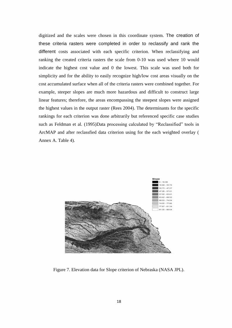
18

digitized and the scales were chosen in this coordinate system. The creation of

these criteria rasters were completed in order to reclassify and rank the

different costs associated with each specific criterion. When reclassifying and

ranking the created criteria rasters the scale from 0-10 was used where 10 would

indicate the highest cost value and 0 the lowest. This scale was used both for

simplicity and for the ability to easily recognize high/low cost areas visually on the

cost accumulated surface when all of the criteria rasters were combined together. For

example, steeper slopes are much more hazardous and difficult to construct large

linear features; therefore, the areas encompassing the steepest slopes were assigned

the highest values in the output raster (Rees 2004). The determinants for the specific

rankings for each criterion was done arbitrarily but referenced specific case studies

such as Feldman et al. (1995)Data processing calculated by “Reclassified” tools in

ArcMAP and after reclassfied data criterion using for the each weighted overlay (

Annex A. Table 4).

Figure 7. Elevation data for Slope criterion of Nebraska (NASA JPL).

19

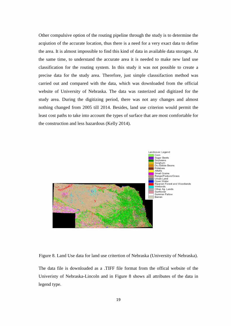
Other compulsive option of the routing pipeline through the study is to determine the

acqiution of the accurate location, thus there is a need for a very exact data to define

the area. It is almost impossible to find this kind of data in available data storages. At

the same time, to understand the accurate area it is needed to make new land use

classification for the routing system. In this study it was not possible to create a

precise data for the study area. Therefore, just simple classsifaction method was

carried out and compared with the data, which was downloaded from the official

website of University of Nebraska. The data was rasterized and digitized for the

study area. During the digitizing period, there was not any changes and almost

nothing changed from 2005 till 2014. Besides, land use criterion would permit the

least cost paths to take into account the types of surface that are most comfortable for

the construction and less hazardous (Kelly 2014).

Figure 8. Land Use data for land use critertion of Nebraska (University of Nebraska).

The data file is downloaded as a .TIFF file format from the offical website of the

Univeristy of Nebraska-Lincoln and in Figure 8 shows all attributes of the data in

legend type.

20

The values were changed only for computation of the landcover. Because, each class

had a different values which is not good for routing. The lowest values were used

with 1, such as agriculutre, other lands and etc; while the highest values mostly were

about water parts and urban places. Since, exploring the study area mentioned that

Keystone XL passed through area mostly covered water recources (The Ogallala

Aquifer) and also there were some small lakes and rivers. Routing the pipeline

through water areas is dangerous and it would cost the construction lots of money.

Given this fact, before planning the routing, it is better to calculate each classes of

the land use just for insurance not to get any problem in the future. Table 3 in the

Annex A displayes how data proccesing prepared for the each weighted overlay

surfaces.

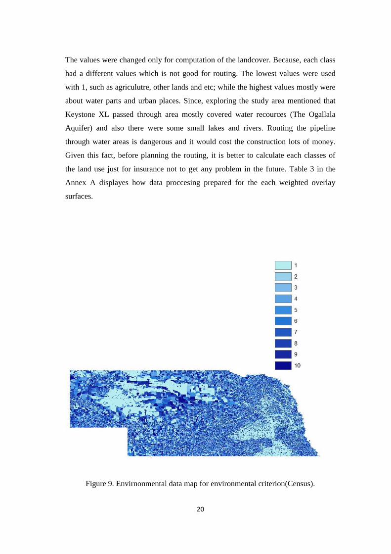
Figure 9. Envirnonmental data map for environmental criterion(Census).

21

The last data facor is about different environmental issues which more concentrated

on the population, houses, block, and etc. The data map have collected by using the

U.S Census TIGER Data Resources and using the ArcMap tools data have been

created for one main data factor. The main goal of the using the environmental

criterion is because to protect state from different kinds of the hazards. Each year in

different states of the U.S some hazards calculated arround 1-2 billion dollars

because of the various hazards (oil spills, gas leaks or natural hazards such as

hurricane). Hence, data try choosed to protecting the study area from hazards and

during routing period to not make some cunstructural affects to the environments.

The spatial resolution was set to the same as the slope and lithology rasters and the

raster was clipped to the extent of the study area. The water bodies’ raster was then

reclassified in the same 1-10 but much differently from the other criteria rasters.

Figure 8 displays environmental data converted to raster file and following figure

also displays result after reclassfying. About data values more detailed information

shown in the Annex A. Table 1.

4.3 Accumulative Cost Surface

The combination of the each criterion rasters in order to create least cost path was

separated into two different techniques. First of all, criterion resters combined

together with equal weighting, where each of the 4 factors calculated with 25 percent

of the influence for routing procedure. In this case each criterion was ranked in a

similar scale and clipped only for the same geographical location. The second

technique generally was divided into four different weighted overlay criterions. Each

overlay was accounted with a different effectiveness percentage. All those processes

were taken from varios studies and from some reports which related exactly the same

topic and also relevant studies discussed in literature review part (Saha 2005;

Geneletti and Orsi 2011). Consequently, each criterion was weighted with specific

22

amount of percentage and then combined together for creating a cost accumaltve

surface using the map algebra. All of the weighted criterions of the four criteria were

collected inside of 100%.

Except the equal weighting overlay, other weighted overlays accounted for each

specific criterions in order to determine and understand the difference between

propoesed pipeline and least cost pathes.

For the first weighted overlay is mostly about the elevation model of the region. With

accurate slope criterion it would help to define the heavy slopes and topographical

partiality of the region. The terrain which includes vertical slopes are more

acceptable to fail.

The second weighted overlay more is about geological stability and geology of the

area. The geological segment has a big role for the routing pipeline. It would help to

predict the area about natural hazards and protect from future hazards. The

geological overlay part is determined from USGS that provides compositions and

age.

The third overlay adopts the land use charasteristics of the study area. The land use

had a more detailed information about the study area. Almost all natural and

agricultural criteria are combined insde of this criterion. It could help constructors to

determine more suitable places and protect agricultural areas from future hazards

such as oil spills and etc.

The study area limited in each specific criterion and also other limitations were about

to figure out the resolution of the each raster datasets and making them more suitable

for applied study area. Resolutions of each cell were different in each raster format,

also other datasets such as population and geology datasets were converted to raster

and cell of each of raster formats modified as a resolution of the elevation data and in

order to get effective costs it was very useful to understand that.

During analyzing of the weighted overlay surface and reclassifyng period there were

some necessery issues such as “NO DATA” values. In each category (except land

use criterion) there were values which displayed as “NO DATA” value. It was

23

displaying in the map some how it can make confusion with error of the cell. Note

that ‘No Data’ cells are excluded from the possibility of travel. The procedure

described “ensures that the lowest accumulative cost is guaranteed for each cell”.

Therefore, cost assigned to every link reflects a resistance value of moving over one

geographic distance unit (ESRI Desktop Help and Belka 2005). More formation

about data processing for each criterion detailed in Annex A.

4.4 Least Cost Routing Tool

After the creation of cost accumulative surfaces using the ArcGIS, least cost tool and

cost path were handled to define the least cost rout through the study area. The

source and destionation points were appointed to the accumulated cost surface based

on the proposed pipeline. The source point was located in the North-West part of a

city which was called Key Paha and the destination point was located in the South

part of Steele city. It was not possible to get point by downloading or searching, so

the special vector data inside Keyston XL geodatabase was made. The starting and

ending points were used due to the accumulated cost surfaces and had the role to

control them as an input and output location inside of the model. Afterward, next

stages were to understand roles of cost distance tool and backling rasters, while these

rasters were used in conjuction inside of cost path tool to create a linear feature

between source and destination point.

The created routes were compared with proposed linear feature and helped to

determine suitable route for weighted overlays. The routes were created with

different weights for each criterion, in order to identify which geographic locations

had more influence and which were most effected by each criterion. All those

methods were taken from different GIS recources and studies which related to the

same topic, such as Kelly 2014 and Saha 2005.

24

5. Result

5.1 Equal Weighted Overlay

The initial cost surface that was generated combined all 4 criteria (slope, geology,

population, and land use) for pipeline routing equally where each criterion accounted

for 25% of the total cost value per cell. The four factors as stated in previous sections

generated a continuous cost surface across the study area that is displayed in Figure

9.

25

Figure 10. Equal Weight cost surface that was formed for the study area.

26

Figure 11. Equal Weighted LCP and straight-line route, which achieved for cost

surface Equal Weights overlay.

In the Figure 10, the green areas define the highest values which this places are not

suitable for routing. Moreover, the map shows the less risky areas that contributed

with the dark brown color. For the reason that the percentage and route corridor

would be more proficient for the overlay, which classified with the equal percentage

effectiveness.

27

Table 1. Least Cost route lengths and Euclidean Path route length, which based on

Equal Weighted Cost surface.

This study has different values from the different lengths of the routes. The relative

cost was impossible to use as a quantitative measurement of the cost of the pipeline

(Kelly 2014). In addition, straight-line path cost was used as a prototype of the

original pipeline. It was not possible to get GPS points from the original Keystone

XL, as there was no chance to get the relative cost of the Euclidean Path to compare

the effectiveness between both paths. The following Table 1 shows that the LCP is

23.18 km longer than STP. Table 1 displays the units that are associated with each

route and also the percent effectiveness that the least-cost path obtains when

compared to the straight-line path across the same cost surface. The least-cost path is

almost 23 km longer than the straight-line path but is 424 units less indicating that

the least-cost path is 17% more effective

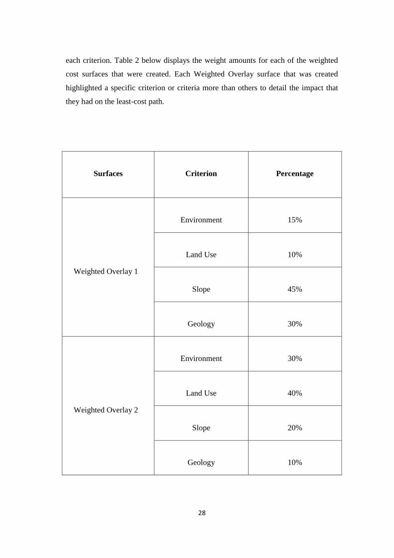
5.2 Weighted Overlays

This part of the study is more about Weighted Overlay surface that had big effective

influences for each specific study field. Multiple cost surfaces were created using the

Weighted Overlay tool in the ArcMap software that designated specific weights to

Route

Length (km)

Units per path

Influence by

percentage

Least Cost Path

423.18

2052

17.1%

Euclidean Path

400.25

2476

28

each criterion. Table 2 below displays the weight amounts for each of the weighted

cost surfaces that were created. Each Weighted Overlay surface that was created

highlighted a specific criterion or criteria more than others to detail the impact that

they had on the least-cost path.

Surfaces

Criterion

Percentage

Weighted Overlay 1

Environment

15%

Land Use

10%

Slope

45%

Geology

30%

Weighted Overlay 2

Environment

30%

Land Use

40%

Slope

20%

Geology

10%

29

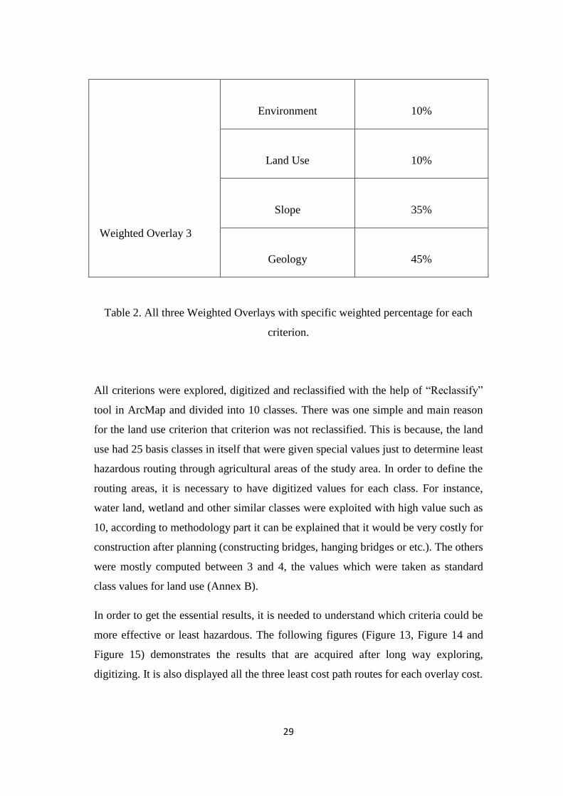
Weighted Overlay 3

Environment

10%

Land Use

10%

Slope

35%

Geology

45%

Table 2. All three Weighted Overlays with specific weighted percentage for each

criterion.

All criterions were explored, digitized and reclassified with the help of “Reclassify”

tool in ArcMap and divided into 10 classes. There was one simple and main reason

for the land use criterion that criterion was not reclassified. This is because, the land

use had 25 basis classes in itself that were given special values just to determine least

hazardous routing through agricultural areas of the study area. In order to define the

routing areas, it is necessary to have digitized values for each class. For instance,

water land, wetland and other similar classes were exploited with high value such as

10, according to methodology part it can be explained that it would be very costly for

construction after planning (constructing bridges, hanging bridges or etc.). The others

were mostly computed between 3 and 4, the values which were taken as standard

class values for land use (Annex B).

In order to get the essential results, it is needed to understand which criteria could be

more effective or least hazardous. The following figures (Figure 13, Figure 14 and

Figure 15) demonstrates the results that are acquired after long way exploring,

digitizing. It is also displayed all the three least cost path routes for each overlay cost.

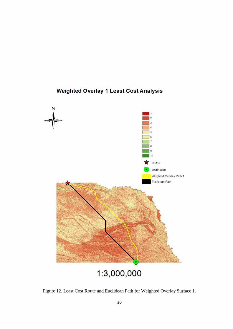
30

Figure 12. Least Cost Route and Euclidean Path for Weighted Overlay Surface 1.

31

Figure 13. Least Cost Route and Euclidean Path for Weighted Overlay Surface 2.

32

Figure 14. Least Cost Route and Euclidean Path for Weighted Overlay Surface 3.

33

Route

Surface

Length (km)

Units per

path

Influence

Percentage

Least Cost

Path

Weighted

Overlay 1

447.28

1867

27.1%

Euclidean Path

Weighted

Overlay 1

400.25

2561

Euclidean Path

Weighted

Overlay 2

421.04

2048

14.7%

Euclidean Path

Weighted

Overlay 2

400.25

2401

Least Cost

Path

Weighted

Overlay 3

515.56

1404

37.0%

Euclidean Path

Weighted

Overlay 3

400.25

2236

Table 3. Least Cost route lengths and Euclidean Path routes length, which based on

Weighted Overlay 1, Weighted Overlay 2 and Weighted Overlay 3 cost surfaces.

34

The costs for the straight-line paths through each of these cost surfaces are higher

than the costs for the least-cost paths, although the lengths of the least-cost paths are

longer. By examining each Weighted Overlay surface one can see that the highest

percent effectiveness was calculated from the third weighted overlay surface with its

value of 37% The third weighted overlay surface placed emphasis on the geological

hazards within the area more so than any of the other criteria. This indicated that the

major criteria for the routing in this study region were the geological hazards that are

present. The Least Cost Path 2 concentrated on the Weighted Overlay which has

more influences from Environmental and Land Use criterion. It is because of the

most environments and agriculture located on the middle part of the study area.

Location of this both criterion is in the high plains area which is very useful for

agriculture and that is why, result displayed 14.7% (less than compare other results).

LCP 1 displayed average result compare Weighted Overlay 1 and 2. Because, more

slopes of the area more upper in the middle and west part of the East part of

Nebraska but effectiveness of geology criterion effect cannot let to analyses to route

path from the East part it is therefore, LCP 1 displayed 27.1% more effective

compare with Euclidean Path.

There can be some confusion about LCP 2 that route passing through area where

there is no data calculated. In the Annex B. Figure 1 displays more details about this

issue. All analyses behaved perfectly and more accurately according to the data sets.

5.3 The Ogallala Aquifer and Proposed Keystone XL Route.

The Keystone XL pipeline was proposed by Trans Canadian Corporation and the

available data can be taken from ESRI. As previously mentioned, the following

details about the data was not with special GPS points or with essential details and it

was not possible to determine main differences between proposed pipeline and least

cost path routes. It is because of the fact that the construction and surveying part of

35

the project has not started yet. As a result, it is not possible to get further information

about the data. The proposed pipeline and least cost route features are shown in

Figure 15 with reclassified slope surface. In this slope surface, the legend is a little

bit different from the previous figure legends. The white parts of surface display the

lowest slopes in the study area.

Figure 15. The proposed Keystone XL from Trans Canadian Corporation and all

least cost path routes displayed on the slope surface.

36

Due to some problems, it was not possible to compare all pipelines with their further

information. The study was about which routes are more effective and which of least

cost routes pass through the Ogallala Aquifer. The results have been discussed in the

discussion part of the thesis. Another issue was about the study that some of the

routes passing through the area are protected by the State Department of the U.S and

some other governmental organizations. The Ogallala Aquifer has been explored in

the study area part and Table 4 displays that which routes passing through the aquifer

and results shown with percentage of the. The results were expectable from my side

of view. So, the least cost path route which was represented on the Weighted Overlay

surface 3 was more effective and less hazardous compared to the other routes and

proposed pipeline.

Surface

Length of the routes,

which passed through,

protected area. (km)

Percentage

Weighted Overlay 1

LCP route

303.54

68%

Weighted Overlay 2

LCP route

358.43

85%

Weighted Overlay 3

LCP route

210.56

40%

Equal Weighted Overlay

325.36

77%

37

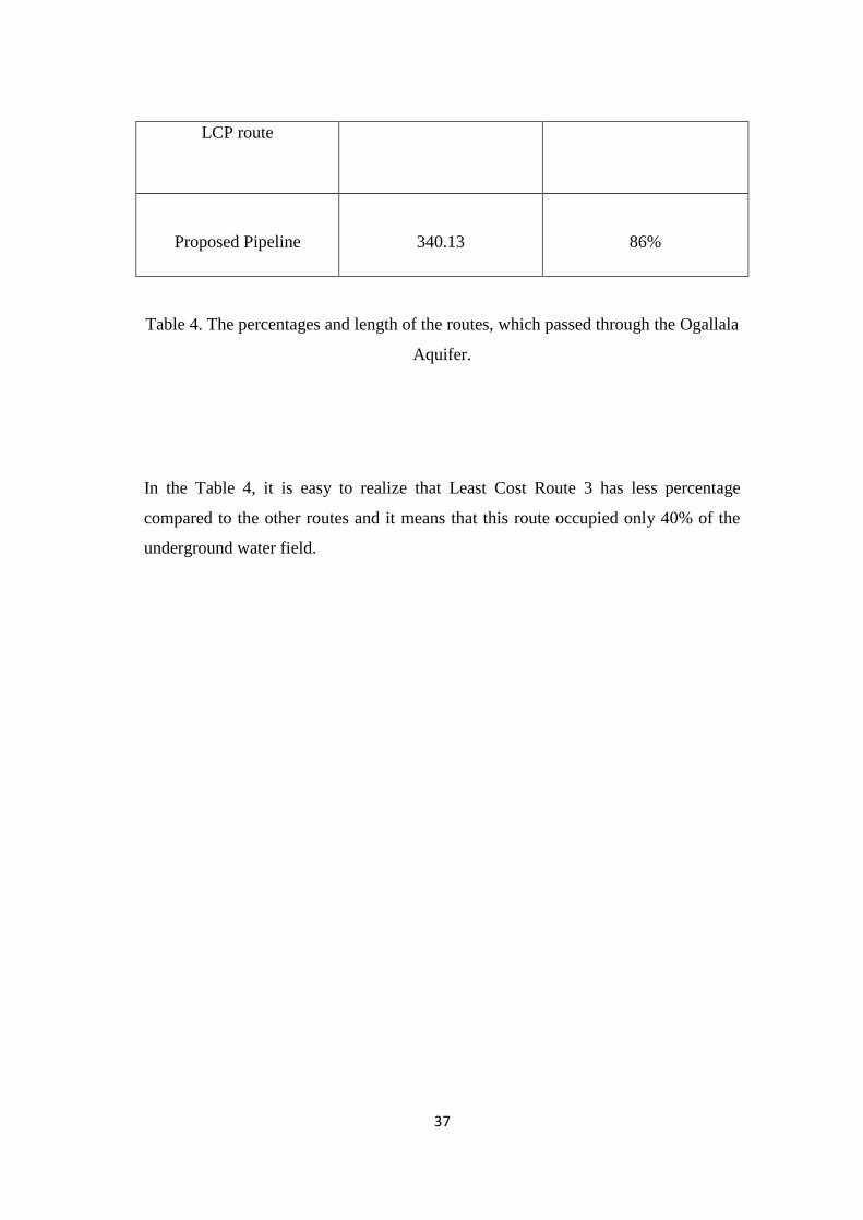
LCP route

Proposed Pipeline

340.13

86%

Table 4. The percentages and length of the routes, which passed through the Ogallala

Aquifer.

In the Table 4, it is easy to realize that Least Cost Route 3 has less percentage

compared to the other routes and it means that this route occupied only 40% of the

underground water field.

38

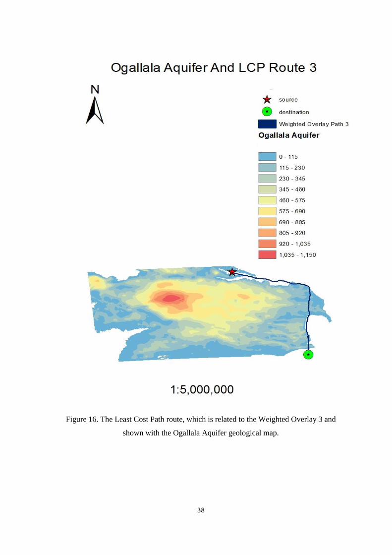
Figure 16. The Least Cost Path route, which is related to the Weighted Overlay 3 and

shown with the Ogallala Aquifer geological map.

39

The following Table 4 and Figure 16 gives accrued results about less hazardous

routes and it shows which the least cost path route based on the Weighted Overlay 3

was more effective and less hazardous. During the calculation time, the units gave

almost 2 time more units than straight-line path, but effectiveness of the route 37.0%.

It is also clear that the weighted overlay 3 was more concentrated on the geology

criterion and it means that the data covers the quality of the high level 9 for the study

area. Detailed lengths and costs were calculated by usage of the ArcMap with

specific coordinate system, projection type and the scale. This criteria is one of the

main purposes of the study.

40

6. Discussion

During the examination period the results were composed from the different four

cost surfaces within the study clearly showed that the least cost tool is more effective

then compare with a normal Euclidean Path. Euclidean Path chosen for as a

prototype of the proposed Keystone XL and generated between two points (source

and destination). It is because of during the study, it was not possible to get an

available exact data about proposed pipeline which is concentrated on the usual GPS

points. Starting with the Equal Weighted cost surface, least cost path route detailed

units were around 17% lower than standard Euclidean Path. According to the Austin

Kelly., 2014, this is not the case though due to the specific criteria that were

combined together to form the cost surface. This is where the logic of the least-cost

algorithm that is coded within the ArcGIS tool displays its worth in navigating the

highest cost cells while traversing the cost surface from source to destination. (Kelly

2014)

The cost that are accumulated for each derived path are not numerical figures that

can be used in projects. For example, in engineering methods as these values only

helping to determine the units of each cost that is generated from transom of the

specific cost surface. The units of the costs displayed on the Table 1 for Equal

Weighted cost surface and Table 3 for following Weighted Overlays. It is also

appropriate to note that the units of the each path costs that were calculated for Equal

Weighted Overlay cannot be comparable with other Weighted Overlay’s results. It is

because of the factors of Equal Weighted Overlays divided between equal percentage

effectiveness but Weighted Overlays have their own specific effectiveness values

which generated on specific values. Another point that issue to according to Kelly

2014, is about different scaling of the cost units between two types of surface (Equal

Overlays and Weighted Overlays).

When the effectiveness of each path routes were compared to another the higher the

effectiveness of the routes, the better routes were crossing through the specific cost

41

surfaces. In displayed table 3 the least cost path was made across Weighted Overlay

3 was the most efficient route to compare with the Euclidean Path. Actually, all of

results behaved in very nice way but the thing is that each routes were dependent on

their specific criterion. The percentages of the each criterion have gotten after few

analyses period which have given by ArcMap. Initial steps about feedbacks of the

each criterion were random and then with starting the analyses feedbacks changed

according to their accumulated cost cells. In this case, Weighted Overlay 3 cost

surface percentages feedbacks were getting by their cost and table 3 it is more

detailed. Weighted Overlay 3 more effective by geologic values of the units which is

more concentrated about lithology, rock, water resources and etc. in the study area.

The Least Cost Path 3 was more effective to compare with other overlay surfaces and

supposedly it is because of the data was more accurate for the region. It is already

clear that in the study are there is a big aquifer which has influences for the Least

Cost Path and I was one of the main goal to determine the route which is not passing

through the aquifer area. The available data set downloaded from the USGS official

website and Conservation and Survey Division (CSD) provided this data more

beneficial. CSD provided beneficial dataset which had beneficial effect on the study.

They engaged in geologic mapping, researches about soils, settlings of different

rocks and etc. Studies conducted by CSD personnel provide the basis for effective

resource management and use, water resource safety and security, the exploration

and exploitation of industrial mineral and fuel resources, natural-hazard mitigation,

and building-site evaluation (University of Nebraska 2015). The Least Cost Path

which generated on the Weighted Overlay 3 cost surface and it is more effective

compare with Euclidean Path and other LCP routes percentage. Secondly, only 40%

of the route passing through protected the Ogallala Aquifer and in this issue also has

more effective result to compare with other routes.

Another main issue were concentrated to find out the route which cannot make land

slide and terrain hazards for the study area. Weighted Overlay 1 cost surface more

concentrated on the slope criterion and feedback percentage about weighted overlays

have same methodology which explained in previous part. From the study area part

of the thesis it is almost understandable that in the following region terrains are not

42

higher than the West part of Nebraska State and study generated on the East part that

is why, level alttidue less than the Middlewest of Nebraska. The elevation data

downloaded from official website of the NASA JPL and digitized for the study area.

The results showed that LCP 2 was 14% cheeper and less hazardous compare with

the Euclidean Path but this route connot apply for construction. Because, 68% of the

least cost path route croosing through the Ogallala Aquifer. Compare it to Equal

Weighted and Weighted overlay 2 it is seems more suitbale but compare it with LCP

3 that the route LCP 1 is more longer.

The latest overlay is displaying agricultural and evinormental issues for Nebraska

State. The mostly agricultural issues located in the central parts of the study area and

it is because of the high plain location. Ususally agricultural areas are locating on the

area which is suitable for them. Following Weighted Overlay 2 more concentrated

about agricultural issues and from the Figure 13 it is more visible that central areas

are more about this criterion. Dataset for the this criterion downloaded from

University of Nebraska-Lincoln which is providing accurate and available data sets

for Nebraska state. It does not make sense to provide criterion more about population

areas, it is because of the study area population calculated around 2 million and

heavy population more located in the Midwest and kind of central area and

environmental data is not providing exact data about population there includes

houses and block into environmental critertion.

Land use criterion data just digitized only for study area but it did not pass though

the reclassification period. It is because, dataset was providing small amount of

atrributes and it was easy to numerized it by manually. In the Annex A Table 3

displays values which choosen manually and the goal it was about to route the

pipeline thorugh the water areas. Because, water sources are more expensive and

more hazardous for construction. The result from table 3 shows that the Least Cost

Path which generated on Weighted Overlay 3 is 14% effective compare with staright

line path which generated in the same overlay cost surface. It can be 14% cheeper

that Euclidean Path but again it connot be applicable for the region. Because, only

85% of route passing through protected area and it is just 1% less than proposed

Keystone XL.

43

A key maintenance to take into account when examining the results from the

proposed

Keystone XL route and the least cost routes that were practically created was that

even though these practical routes only took into account a very selected few criteria

they almost simulated the proposed route. In Figure 12 shows that the eximined

routes were sourced from the exact location where the proposed route inputted the

study area. This is not due to the changing condition when routing large projects such

as this pipeline. Although the source locations for each route were different, this did

not affect the practical routes significantly enough to document.

Another key limition of this study was about the obtaining more accurate data for

Nebraska State. It is not possible to understand how and which datasets used by

Transcanadian Coorpoartion to propose Keystone XL but in case of the study all

datasets were more accurately and they behaved from the begining which results

were expecting. Only problem about original data for proposed Keystone XL. It

needed because to understand atrributes and make more observations for area which

is proposed Keystone XL crossed. There were “No Data” values for the each

Weighted Overlays and they were locating mostly middle and right part of the study.

It was not about error or some factors which cannot effected to surface to route paths

through the region.According to Belka., 2005 it is normal to get “No Data” values

and it is only because of the reclassification of the factors (except land use).

44

7. Conclusion

The created least-cost paths from this thesis provides the least hazardous pipeline

routes by using the available data that covers the region of Nebraska State. When

comparing the created routes to the proposed Keystone XL the least-cost paths

accurately detail routes that are strikingly similar and effective in providing a path

from the documented source and destination points within Nebraska. This thesis,

using similar studies as background and for reference, combined the key factors in

routing a large-scale pipeline project into a relevant cost surface that was then able to

perform a least-cost path analysis and deliver a connected route. While the thesis had

some limitations with the amount of data available and its precision, the overall

result was a viable least-cost path that satisfied the main regulations with routing this

type of infrastructure.

The study concentrated on the four different weighted overlays and demonstrated

with different least cost paths routes which helped to determine least hazardous route

for the study area. The results were more precision compare with proposed pipeline

and it could be more accurately with more precision data sets. Least Cost Path

analyses distributed in various criterion which last results (Table 2) of the each

criterion calculated by logic of the algorithm.

Results of the thesis were behaved more proper way in true sense of the word,

especially Least Cost Path analyses which related to Weighted Overlay 3 and result

will help in future to determine route with more proper and least hazardous way.

45

Bibliographical References

1) Mahmoud Reza Delavar, Fereydoon Naghibi., 2005, Pipeline Routing Using Geospatial

Information System Analysis.

2) M.F. Goodchild., 1976, An evualation of lattice solutions to the problem of corridor

location.

3) Abdul-Lateef Balogun, Abdul-Nasir Matori, Khamaruzaman Yussof, Dano Umar Lawal,

Imtiaz Ahmed Chandio., 2012, GIS in Pipeline Route Selection: Current Trend and

Challenges.

4) Volkan Yildirim, Tahs in Yomralioglu., 2012,GIS Based Pipeline Route Selection by

ArcGIS in Turkey.

5) Volkan Yildirim, Recep Nisanci, Selcuk Reisş, October 8-13, 2006, A GIS Based Route

Determination in Linear Engineering Structures Information Management (LESIM). Shaping

the Change XXIII FIG Congress Munich, Germany.

6) Maheen Iqbal, Farha Sattar, Muhammad Nawaz., 2006 IEEE, Planning a Least Cost Gas

Pipeline Route A GIS & SDSS Integration Approach.

7) Imtiaz Ahmed Chandio, Abd Nasir B Matori, Khamaruzaman B WanYusof, Mir Aftab

Hussain Talpur, Dano Umar Lawal, Abdul-Lateef Balogu., Routing of road using Least-cost

path analysis and Multi-criteria decision analysis in an uphill site (Development. Department

of Civil Engineering, Universiti Teknologi Petronas, Seri Iskandar, 31750, Perak, Malaysia).

8) Avinash Kumar, S.K. Ghosh, Dr. Mili Ghosh, Kishore Kumar, Siddhartha Khare., 2012,

Pradeep Chaudhry GIS based planning for finding optimal gas pipeline route in IITR campus.

(Department of Civil Engineering, IIT Roorkee and Department of Remote Sensing, BIT

Mesra, Ranchi. Paper Reference Number: PN-131. INDIA Geospatial Forum).

9) Kristen Shreen, Noah Enelow, Jeremy Brecher, Brendan Smith., 2013, (The Keystone

Pipeline Debate)

46

10) www.Keystone-xl.com

11) Fotios G., 2011, Method for route selection of transcontinental natural gas pipelines.

Thomaidis.National and Kapodistrian. (University of Athens Department of Informatics and

Telecommunications).

12) Aissi, Hassene, Salem Chakhar, Vincent Mousseau., 2012, GIS-based Multicriteria

Evaluation Approach for Corridor Siting. (Environment and Planning B-Planning & Design 39

(2): 287–307. doi: 10.1068/b37085).

13) Collischonn, Walter, Jorge Victor Pilar., 2000, A Direction Dependent Least-costpath

Algorithm for Roads and Canals. (International Journal of Geographical Information

Science).

14) Dijkstra, E. W., 1959. A Note on Two Problems in Connexion with Graphs.

(Numerische Mathematik 1 (1): 269–71. doi: 10.1007/BF01386390).

15) Feldman, Sandra C., Ramona E. Pelletier, Ed Walser, James C. Smoot, Douglas Ahl.,

1995, A Prototype for Pipeline Routing Using Remotely Sensed Data and Geographic

Information System Analysis. (Remote Sensing of Environment).

17) Lee, Jay, Dan Stucky., 1998, On Applying View-shed Analysis for Determining Least-

cost Paths on Digital Elevation Models. (International Journal of Geographical Information

Science).

18) Rees, W.G., 2004, Least-cost Paths in Mountainous Terrain. (Computers &

Geosciences. 2003).

19) Saha, A. K., M. K. Arora, R. P. Gupta, M. L. Virdi, E. Csaplovics. 2005. GIS•based

Route Planning in Landslide Prone Areas. (International Journal of Geographical Information

Science 19 (10): 1149–75).

20) Yang, Si-Zhong, Hui-Jun Jin, Shao-Peng Yu, You-Chang Chen, Jia-Qian Hao, Zhen-

Yuan Zhai., 2010, Environmental Hazards and Contingency Plans Along the Proposed

China–Russia Oil Pipeline Route, Northeastern China. (Cold Regions Science and

Technology 2009).

21) August 2004, MEDGAZ Natural Gas Transportation System ENVIRONMENTAL

IMPACT ASSESSMENT (Final Report).

47

22) Kamila Małgorzata Belka., 2005, Multicriteria analysis and GIS application in the

selection of sustainable motorway corridor.

23) Abdul-Lateef Balogun., 2013, Geographic Information System (GIS) in Offshore Pipeline

Route Selection: Past, Present, and Future. (Department of Civil Engineering, Universiti

Teknologi PETRONAS (UTP), Perak, Malaysia.).

24) Mahmoud Reza Delavar, Fereydoon Naghibi., 2009, Pipeline Routing Using Geospatial

Information System Analysis.

25) Eurostat. 2007. (Eurostat Statistical Books - Gas and Electricity Market Statistics).

26) Denise Chow, Staff Writer., 2013, Water Woes: Vast US Aquifer Is Being 27)Tapped

Out. (URL: http://www.livescience.com/39186-kansas-aquifer-water depletion.html)

28) Austin Kelly., 2014, GIS Least-Cost Route Modeling of the Proposed Trans-Anatolian

Pipeline in Western Turkey (Georgia State University).

29) Brad Plumer., 2015, 9 questions about the Keystone XL pipeline debate you were too

embarrassed to ask. (URL: http://www.vox.com/2014/11/14/7216751/keystone-pipeline-

facts-controversy).

30) University of Nebraska. School of Natural Recourses. Collage of Agricultural Sciences

and Natural Recourses.

31) Communication Sciences & Disorders (CSD) Education Survey Nebraska Aggregate

Data Report 2012-2013 Academic Year.

32) Xiaoge, Z., Wentong, D., 2005, GIS Technology and Application on Oil-gas Pipeline

Construction.(URL: http://ieeexplore.ieee.org/iel5/7719/21161/00982754.pdf).

33) Nasir, M. S, Hyder, S. K., 2001, “Economics of Pakistan”. (New United Booksellers,

Lahore, pp 248)

34) Dubey, R.P., 2005, A Remote Sensing and GIS based least cost routing of pipelines.

(URL: http://www.gisdevelopment.net/application/Utility/transport/utilitytr0025pf.htm).

35) Lovett, Andrew A., Julian P. Parfitt, Julii S. Brainard., 1997, Using GIS in Risk Analysis:

A Case Study of Hazardous Waste Transport. Risk Analysis.

48

36) Luettinger, Jason, Thayne Clark., 2005, Geographic Information System-based Pipeline

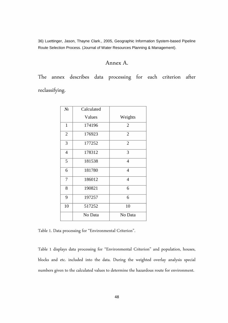
Route Selection Process. (Journal of Water Resources Planning & Management).

Annex A.

The annex describes data processing for each criterion after

reclassifying.

№ Calculated

Values

Weights

1 174196 2

2 176923 2

3 177252 2

4 178312 3

5 181538 4

6 181780 4

7 186012 4

8 190821 6

9 197257 6

10 517252 10

No Data No Data

Table 1. Data processing for “Environmental Criterion”.

Table 1 displays data processing for “Environmental Criterion” and population, houses,

blocks and etc. included into the data. During the weighted overlay analysis special

numbers given to the calculated values to determine the hazardous route for environment.

49

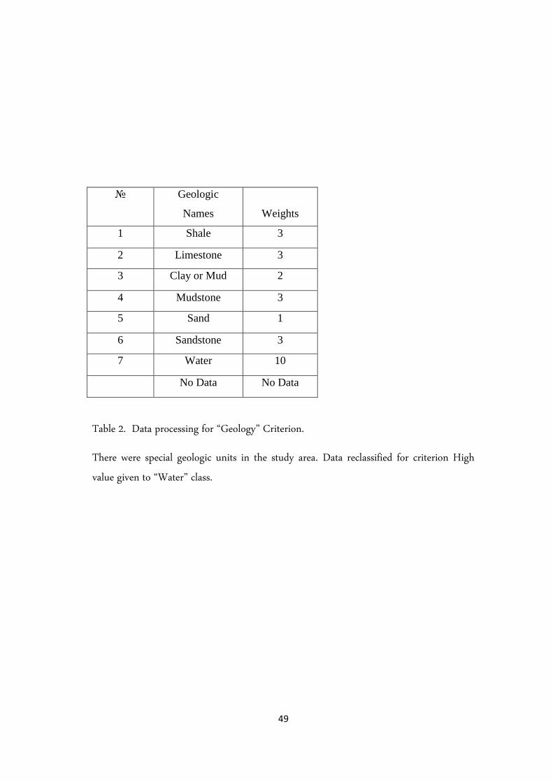
№ Geologic

Names

Weights

1 Shale 3

2 Limestone 3

3 Clay or Mud 2

4 Mudstone 3

5 Sand 1

6 Sandstone 3

7 Water 10

No Data No Data

Table 2. Data processing for “Geology” Criterion.

There were special geologic units in the study area. Data reclassified for criterion High

value given to “Water” class.

50

№ Classes Weights

1 Corn 3

2 Sugar Beets 3

3 Soybeans 3

4 Sorghum 3

5 Dry Edible Beans 3

6 Potatoes 3

7 Alfalfa 3

8 Small Grains 2

9 Range/Pasture/Grass 1

10 Urban Land 5

11 Open Water 10

12 Woodlands 8

13 Other Ag.Lands 3

14 Sunflower 3

15 Summer Fallow 5

16 Barren 1

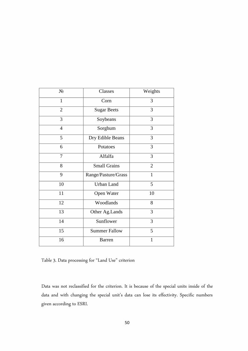
Table 3. Data processing for “Land Use” criterion

Data was not reclassified for the criterion. It is because of the special units inside of the

data and with changing the special unit’s data can lose its effectivity. Specific numbers

given according to ESRI.

51

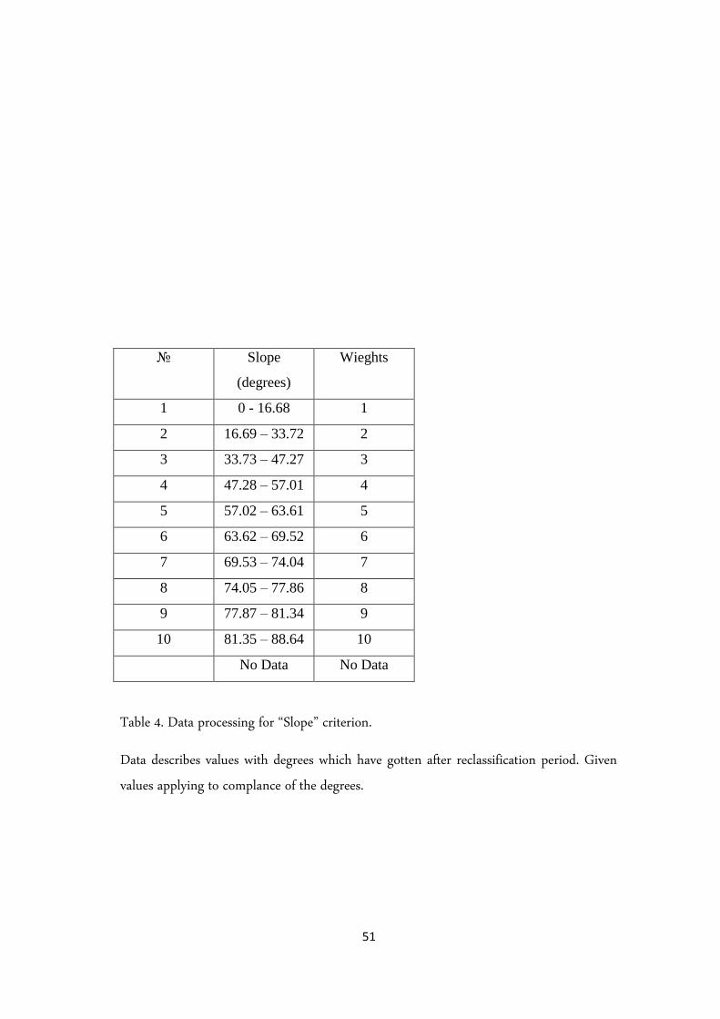
№ Slope

(degrees)

Wieghts

1 0 - 16.68 1

2 16.69 – 33.72 2

3 33.73 – 47.27 3

4 47.28 – 57.01 4

5 57.02 – 63.61 5

6 63.62 – 69.52 6

7 69.53 – 74.04 7

8 74.05 – 77.86 8

9 77.87 – 81.34 9

10 81.35 – 88.64 10

No Data No Data

Table 4. Data processing for “Slope” criterion.

Data describes values with degrees which have gotten after reclassification period. Given

values applying to complance of the degrees.

52

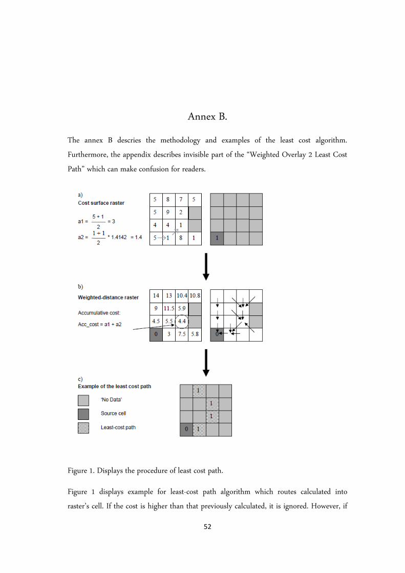
Annex B.

The annex B descries the methodology and examples of the least cost algorithm.

Furthermore, the appendix describes invisible part of the “Weighted Overlay 2 Least Cost

Path” which can make confusion for readers.

Figure 1. Displays the procedure of least cost path.

Figure 1 displays example for least-cost path algorithm which routes calculated into

raster’s cell. If the cost is higher than that previously calculated, it is ignored. However, if

53

the cost value is lower, the old accumulative cost is replaced. The cells that are already

assigned to the output raster are not recalculated and treated as ‘permanent’. The process

is repeated until the least accumulative cost is assigned to all cells and the back link raster

is completed. Generation of the weighted-distance raster is based on graph theory and the

shortest path is based on the Dijkstra algorithm (ESRI Desktop Help and Belka., 2005).

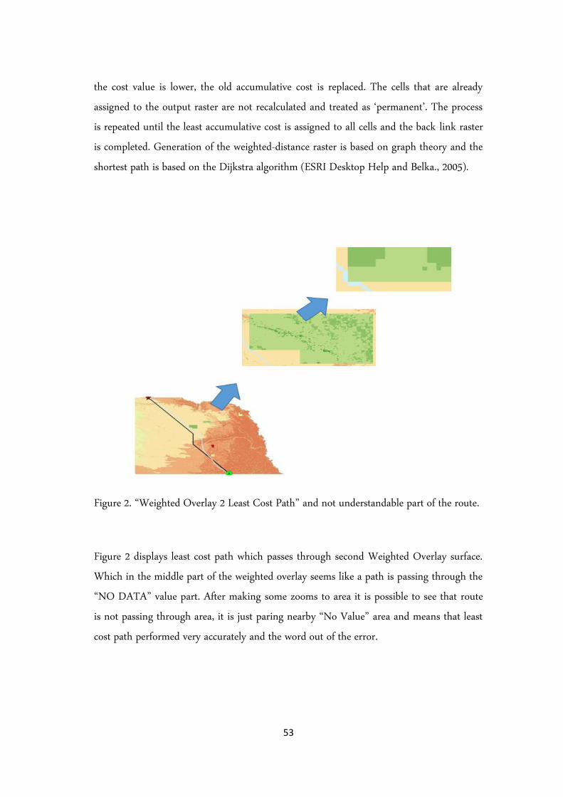
Figure 2. “Weighted Overlay 2 Least Cost Path” and not understandable part of the route.

Figure 2 displays least cost path which passes through second Weighted Overlay surface.

Which in the middle part of the weighted overlay seems like a path is passing through the

“NO DATA” value part. After making some zooms to area it is possible to see that route

is not passing through area, it is just paring nearby “No Value” area and means that least

cost path performed very accurately and the word out of the error.

54