1

Determination of the influence of machining defects

on the magnetic field as a part of the design of new

magnets for the CEBAF 12-GeV upgrade

Nicolas Ruiz

Direction: Jay Benesch

Abstract

In order to eventually guide the electrons throughout the accelerator up to their highest

energy, the beam trajectory has to be simulated for the entire accelerator with

appropriate numerical codes, such as ELEGANT, Optim, etc. prior to the actual facility

construction. In the 12 GeV project framework, constraints are tighter than they were

for the 6 GeV machine and the accuracy of the simulations have to catch up. Since

measured data concerning the elements are not available in many cases, local scale

simulations acquire a very particular importance for they can be the only way available

to determine the characteristics that will be used to introduce each magnet into whole-

accelerator simulations. The present study focuses on a possible improvement of those

local simulations by making them take into account more realistic parameters such as

machining defects.

The local scale simulation tool used in this study takes a large number of characteristics

of the magnets into account. However, none of the simulations realized so far included

geometry imperfections. The poles were assumed to be perfectly parallel, their surface

to be perfectly plane... Those assumption appeared to be valid up to now, but since both

fields and steel saturation in the magnets of the 12 GeV-configured lattice are going to

be much higher than in the present 6 GeV machine, the idea of taking geometrical

imperfections into account arose from the concern of being able to precisely specify the

tolerances that were to be required for the new magnets.

The first models comprising simulations of machining defects are created throughout

this study, and a valid perturbation modeling technique is developed. A strong

correlation is observed between the first skew multipole terms of the field and the

amplitude of the geometrical perturbation and conclusions are drawn concerning the

field perturbations induced in the zone located between the magnet poles. However, the

mesh densities reached at the time of this study and the field evaluation techniques that

were exploited did not allow to draw conclusions regarding the influence of the edges of

the magnet poles whose study remains for further work on the subject.

Discrepancies between the actual values of the simulated field perturbations and the

measured data that is available are addressed and some advice is dispensed concerning

future parts specifications and assembly. The final word however recalls that actual

direct measurements of what was simulated are of course desired to qualify the results

and the conclusions.

2

Introduction

This document presents the work realized by the author for his master thesis under the

direction of Jay Benesch. It is divided in six main parts.

The two first parts explain the origins of the concern founding this study as well as the

strategy that was elected in order to establish conclusive results. The third part relates

step by step the proceeding that has been followed, in accordance with the above

mentioned strategy. Part four presents the results of the study along with their

interpretation. The practical conclusions that can be deduced from those results are

listed in part five. References, bibliography and annexes constitute the sixth and last

part of this document.

Note: Out of concern for consistency with the scientific procedures being followed

among the physicists at Jefferson lab, every value in this document is given in the CGS

unit system, unless explicitly indicated otherwise.

3

Table of contents

II -- IInniittiiaall ccoonncceerrnn ............................................................................................................ 4

I.1 - Initial situation ....................................................................................................... 4

I.2 - Objective of my work ............................................................................................. 4

IIII -- SSttrraatteeggyy ..................................................................................................................... 6

IIIIII -- TTeecchhnniiccaall ddeessccrriippttiioonn ooff tthhee ssttuuddyy ........................................................................ 7

III.1 - Description of the modeling environment .......................................................... 7

III.1.1 - Software resources ................................................................................... 7

III.1.2 - Morphing tools ......................................................................................... 8

III.1.3 - Hardware resources .................................................................................. 9

III.2 - Description of the part chosen for the study .................................................... 10

III.2.1 - Context ................................................................................................... 10

III.2.2 - Magnet description ................................................................................. 10

III.2.3 - Criteria for the choice ............................................................................. 11

III.3 - Geometrical specifications of the original part ................................................. 12

III.3.1 - Concern .................................................................................................. 12

III.3.2 - Tolerances .............................................................................................. 13

III.4 - Finding a 'worst' machining case ....................................................................... 15

III.4.1 - Concept .................................................................................................. 15

III.4.2 - Presentation of the model ....................................................................... 16

III.4.3 - Perturbations applied .............................................................................. 17

III.5 - Field evaluation method .................................................................................... 18

III.5.1 - Definition of multipoles ......................................................................... 18

III.5.2 - Measuring multipoles ............................................................................. 21

III.5.3 - On skew multipoles ................................................................................ 24

IIVV -- RReessuullttss .................................................................................................................... 25

IV.1 - Effect of the introduction of a perturbation ..................................................... 25

IV.1.1 - Presentation of the original model ......................................................... 25

IV.1.2 - Analysis of the perturbed model ............................................................ 25

IV.1.3 - Comparison with a full-height, non-perturbed model ............................ 29

IV.1.4 - Comparison with other perturbed models .............................................. 31

IV.2 - Effect of Field Intensity ...................................................................................... 33

IV.3 - Quantitative influence of geometrical perturbations ....................................... 36

IV.3.1 - Models used ........................................................................................... 36

IV.3.2 - Multipoles behavior ............................................................................... 38

IV.3.3 - Relative importance of body and edge fields ......................................... 42

VV -- GGeenneerraall ccoonncclluussiioonnss ................................................................................................ 44

VVII -- RReeffeerreenncceess,, bbiibblliiooggrraapphhyy aanndd aannnneexxeess ................................................................ 45

VI.1 - References ......................................................................................................... 45

VI.2 - Bibliography ....................................................................................................... 45

VI.3 - List of Annexes ................................................................................................... 47

4

II -- IInniittiiaall ccoonncceerrnn

II..11 -- IInniittiiaall ssiittuuaattiioonn

In order to be able to guide the electrons throughout the accelerator as their energy gets

higher and higher, the beam trajectory has to be simulated for the entire accelerator with

appropriate numerical codes, such as ELEGANT, Optim, etc. prior to the actual facility

construction. This has been done for the 6-GeV current configuration of the CEBAF so

that accelerator designers could know in advance where to put the magnets and how to

tune them.

To realize the 12-GeV upgrade, a different configuration is required, with new or

modified parts, higher fields... The constraints are tighter and the accuracy of the

simulations have to catch up.

In whole-accelerator simulations, and because the CEBAF counts more than 2000

magnets, each element cannot be modeled with its entire geometry (coils, steel, current

density...). Instead, each element (magnets, filters...) of the lattice is represented by a set

of relevant numerical values, like the integrated field 'seen' by the particles traversing it

for example, that tells the code how to take into account the influence of this particular

element while it computes the beam trajectory. It's a form of multi-scale modeling.

Those relevant characteristics must be evaluated for each part, as accurately as possible,

since the setup of the whole accelerator depends on it.

The best case occurs when the parts already physically exist and we can make proper

measurements of their characteristics. Unfortunately, measurements take time, and the

equipment necessary to perform them can be expensive and is not always available. As

a result, even in the case of pre-existing 6-GeV parts, many of the characteristics used to

simulate the role of these elements had to be evaluated by simulations instead of being

actually measured.

Moreover, in the 12-GeV upgrade case, many parts are new or modified, so that their

modeling acquires a very particular importance for it is the only way available to

determine the characteristics that will be used for their integration into whole-

accelerator simulations.

The present study takes place in that context, focusing on a possible improvement of

those local simulations by making them take into account more realistic parameters such

as machining defects.

II..22 -- OObbjjeeccttiivvee ooff mmyy wwoorrkk

As the previous section explained, a series of relevant parameters is determined for each

element of the accelerator, either by physical measurement or by simulation of the

element's magnetic field on a local scale, for it to represent the modeled element in

future larger scale simulations.

The local scale simulation tool used in this study (see section II.3.1.1) takes a large

number of characteristics of the magnets into account: the disposition of the coils as

well as their current density, the geometry of the return steel, magnetic properties of the

steel (editable B-H curve), etc.

5

However, none of the simulations realized so far with this tool took geometry

imperfections into account. The poles were assumed to be perfectly parallel, their

surface to be perfectly plane... In other words, no machining or assembly defects were

taken into account while defining the geometry of the modeled magnets. Their influence

on the field dispensed by the magnet was therefore not present in the results of the

simulations, resulting in its not being taken into account in larger scale simulations

either.

Since the fields in the magnets of the 12GeV-configured lattice are going to be higher

than they currently are, thus placing their steel into a saturated state in many volumes,

the idea of taking geometrical imperfections into account arose from the concern of

being able to precisely specify the tolerances that were to be required for the new

magnets.

The objective of this study is to realize the first models that would take machining

defects into account, and to gather information regarding their effect on the magnetic

field. Possible results are:

- a better understanding of the current machine and of what has been neglected

so far

- a finer notion of the correlation between the mechanical tolerances that lab

designers specify for the magnets and the undesired field components that can be

expected to arise from those specifications

6

IIII -- SSttrraatteeggyy

The approach that was first decided is the following. All this process is then detailed

step by step in the next section (II.3- Technical description of the study).

The first step is to get acquainted with the modeling tool and its morphing functions, in

order to be able to introduce geometrical perturbations in pre-existing magnet models.

Then, with the help of my supervisor and according to relevant criteria, a specific

magnet in the lattice is selected for geometric perturbations effects on the field to be

studied using its model. This election is crucial for the results of this study to be of

interest in the design and specification of other magnets.

Once the magnet is chosen and its technical drawing is acquired, design machining

tolerances are evaluated. The idea is to start by determining a tolerance-fulfilling 'worst

machining case' to work on, to have an order of magnitude of the maximum field

perturbation that the current design is allowing. Once again, different scientific criteria

are taken into account in this case election, for geometrical product specification

intrinsically leaves degrees of freedom in part machining.

Chosen geometrical imperfections are then introduced in the original magnet model.

After processing, field calculations reveal, as expected, the apparition of new magnetic

field components, that were negligible in unperturbed models.

The next and concluding step of the study is to try and establish correlations between

the perturbations introduced and the induced modifications of the field. This paper

mainly focuses on the amplitude of the perturbations, and relates discovered relations

between magnet machining quality and unwanted field components.

7

IIIIII -- TTeecchhnniiccaall ddeessccrriippttiioonn ooff tthhee ssttuuddyy

IIIIII..11 -- DDeessccrriippttiioonn ooff tthhee mmooddeelliinngg eennvviirroonnmmeenntt

III.1.1 - Software resources

Magnetic calculations

The numerical code used in this study to model geometries and calculate fields is called

Opera 3D. It is written by a British company named Vector Fields [1]. The code has

different modules which correspond to the type of physical values one wants to

calculate (static or varying electric and magnetic fields, thermal and stress analysis... )

and in the present case, the solver used for static magnetic fields is called Tosca.

The scheme for the use of those solvers is the standard pre-processing/solving/post-

processing one. Here it is as explained on the company's website:

The most recent pre-processing tool is called the 'Modeller'. It allows you to create 3D

volumes and perform simple Boolean operations on them or either import the geometry

of your system from another CAD tool. It can also create coils of any shape, and one

defines the current that runs through them. In the end, once the required geometry as

well as the field sources are defined, a mesh generator based on the ACIS kernel fills

the model with finite elements.

Then Tosca, a finite element code, computes the magnetic field in every part of the

model using Newton-Raphson relaxation to deal with the steel, whose magnetic

properties are non-linear.

An example of a calculation report emitted by the code is available in annex [A4].

Fig. II.1: Utilization scheme for the Opera 3D numerical code

Fig. II.2: The Vector Fields logo

8

Post processing

The process used to study the field in the solved models is described in details in section

II.3.5. It uses the Opera 3D post processor for initial field evaluations, whose result are

treated in spreadsheets [2] [3] afterwards. Those have mathematical and statistical

calculation capabilities that are necessary to make the field evaluations exploitable.

Their graphical representation functionalities are also very useful when it comes to

comparing models, fields...

The data coming out of the post processor is converted into a spreadsheet-friendly

format by a Perl script written by the student. An shortened example of a post processor

output file as well as the Perl script are available in annexes [A1] and [A2].

III.1.2 - Morphing tools

Since the objective of the study is to take geometrical imperfections into account, it is

necessary to get familiar with the options offered by the code that can be used to model

such imperfections.

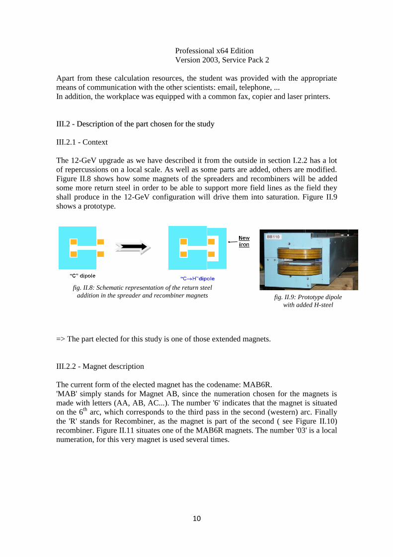
The Opera 3D modeler offers different functions for model distortion.

The main ones are:

- twisting, defining an axe with two points and an angle of torsion

- stretching, again defining an axe with two points and an axial displacement for each

of them

Fig. II.4: twisting operation in

the modeler

Fig. II.5: stretching illustration

fig. II.3: Original Block

used in illustrations

9

fig.II.6: Bended volume

- bending, creating a local coordinate system to

define the bending plane, and then choosing an

angle and a radius for the bend

- the modeler also has a 'general morph'

option, which performs any transformation to each of the coordinates, as long as a

Cartesian equation is available for that function, which must be properly defined in the

treated volume coordinates range.

III.1.3 - Hardware resources

In order to be able to realize the modeling, meshing and solving operations that this

magnetic field fine study requires in good conditions, an appropriate workstation has

been used. The calculations made by the student were realized on a machine with the

following characteristics:

Make : Dell

Model : Precision PWS490

Processor : Intel Xeon X5355 @ 2.66 GHz (QuadCore)

Memory : 16 GB of RAM

Operating system : Microsoft Windows XP

fig. II.7: Example of a general morph. Here the 'Y' coordinate is modified to

follow the curve of an ellipse.

10

Professional x64 Edition

Version 2003, Service Pack 2

Apart from these calculation resources, the student was provided with the appropriate

means of communication with the other scientists: email, telephone, ...

In addition, the workplace was equipped with a common fax, copier and laser printers.

IIIIII..22 -- DDeessccrriippttiioonn ooff tthhee ppaarrtt cchhoosseenn ffoorr tthhee ssttuuddyy

III.2.1 - Context

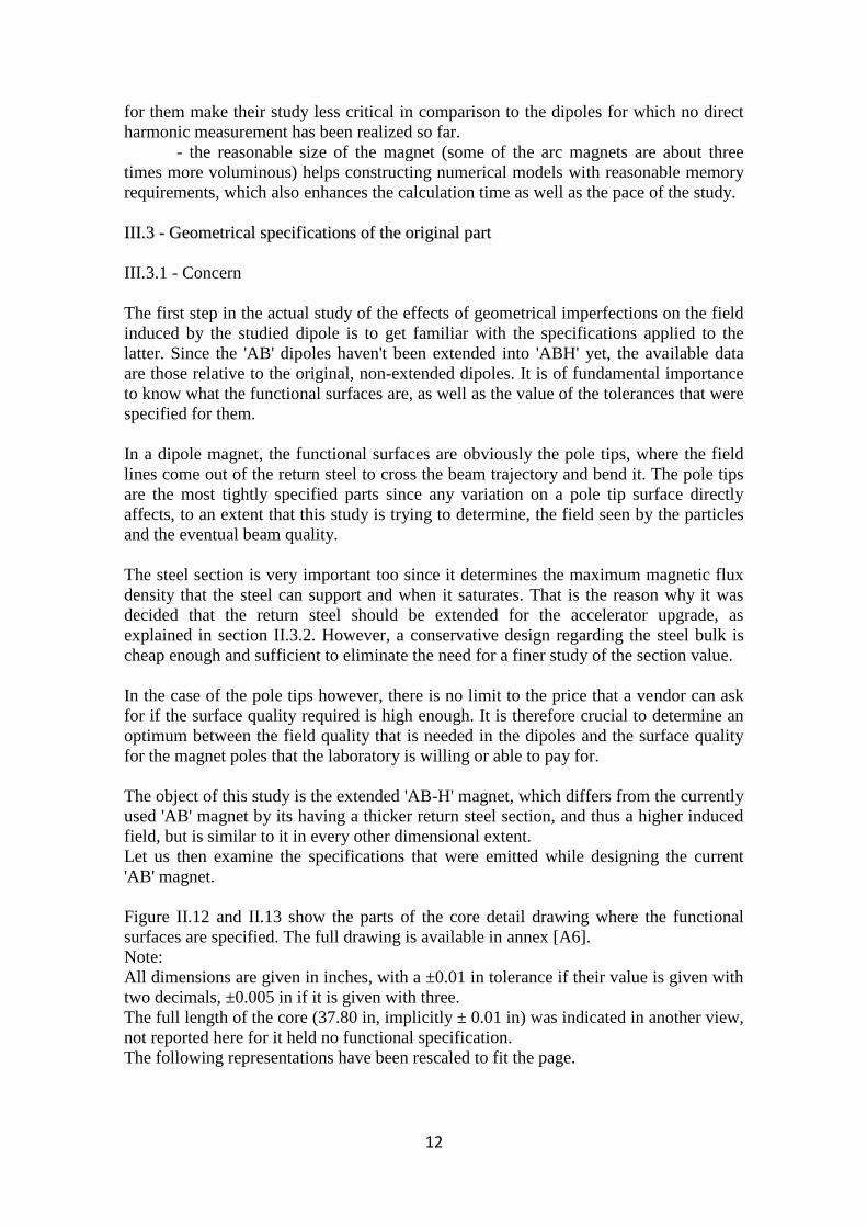
The 12-GeV upgrade as we have described it from the outside in section I.2.2 has a lot

of repercussions on a local scale. As well as some parts are added, others are modified.

Figure II.8 shows how some magnets of the spreaders and recombiners will be added

some more return steel in order to be able to support more field lines as the field they

shall produce in the 12-GeV configuration will drive them into saturation. Figure II.9

shows a prototype.

=> The part elected for this study is one of those extended magnets.

III.2.2 - Magnet description

The current form of the elected magnet has the codename: MAB6R.

'MAB' simply stands for Magnet AB, since the numeration chosen for the magnets is

made with letters (AA, AB, AC...). The number '6' indicates that the magnet is situated

on the 6th

arc, which corresponds to the third pass in the second (western) arc. Finally

the 'R' stands for Recombiner, as the magnet is part of the second ( see Figure II.10)

recombiner. Figure II.11 situates one of the MAB6R magnets. The number '03' is a local

numeration, for this very magnet is used several times.

fig. II.9: Prototype dipole

with added H-steel

fig. II.8: Schematic representation of the return steel

addition in the spreader and recombiner magnets

11

N

fig. II.10: Scheme of the CEBAF indicating the

positions of the spreaders and recombiners.

As the magnet is studied here in its extended form, its name is abbreviated in ABH,

where the letter 'H' denotes the fact that this 'C' magnet is somewhat made an 'H' magnet

by its being extended. The engineering drawings for the original magnet and its return

steel respectively bear numbers 22161-0101 and 22161-0002 [8].

III.2.3 - Criteria for the choice

The main criteria that has led to the election of the MAB6R magnet is that once

extended to meet the 12-GeV lattice requirements it will be the magnet with the

strongest field in the whole lattice (~14kG). It was therefore assumed that any effect of

the geometrical perturbations that were to be taken into account in this study would be

magnified by the steel saturation.

A couple of other arguments added to this choice's interest:

- the geometry of this dipole is rather abundant, as more than 30 other dipoles in

the lattice only differ from it by their current density. Since an evaluation of the

correlation between current density and the effects of machining defects enters in this

study, the latter gains in application range.

- although quadrupoles are more numerous in the lattice than dipoles (about

twice as numerous), the number of magnetic field harmonics measurements available

fig. II.11: A part of the second recombiner drawing,

locating an MAB6R magnet

12

for them make their study less critical in comparison to the dipoles for which no direct

harmonic measurement has been realized so far.

- the reasonable size of the magnet (some of the arc magnets are about three

times more voluminous) helps constructing numerical models with reasonable memory

requirements, which also enhances the calculation time as well as the pace of the study.

IIIIII..33 -- GGeeoommeettrriiccaall ssppeecciiffiiccaattiioonnss ooff tthhee oorriiggiinnaall ppaarrtt

III.3.1 - Concern

The first step in the actual study of the effects of geometrical imperfections on the field

induced by the studied dipole is to get familiar with the specifications applied to the

latter. Since the 'AB' dipoles haven't been extended into 'ABH' yet, the available data

are those relative to the original, non-extended dipoles. It is of fundamental importance

to know what the functional surfaces are, as well as the value of the tolerances that were

specified for them.

In a dipole magnet, the functional surfaces are obviously the pole tips, where the field

lines come out of the return steel to cross the beam trajectory and bend it. The pole tips

are the most tightly specified parts since any variation on a pole tip surface directly

affects, to an extent that this study is trying to determine, the field seen by the particles

and the eventual beam quality.

The steel section is very important too since it determines the maximum magnetic flux

density that the steel can support and when it saturates. That is the reason why it was

decided that the return steel should be extended for the accelerator upgrade, as

explained in section II.3.2. However, a conservative design regarding the steel bulk is

cheap enough and sufficient to eliminate the need for a finer study of the section value.

In the case of the pole tips however, there is no limit to the price that a vendor can ask

for if the surface quality required is high enough. It is therefore crucial to determine an

optimum between the field quality that is needed in the dipoles and the surface quality

for the magnet poles that the laboratory is willing or able to pay for.

The object of this study is the extended 'AB-H' magnet, which differs from the currently

used 'AB' magnet by its having a thicker return steel section, and thus a higher induced

field, but is similar to it in every other dimensional extent.

Let us then examine the specifications that were emitted while designing the current

'AB' magnet.

Figure II.12 and II.13 show the parts of the core detail drawing where the functional

surfaces are specified. The full drawing is available in annex [A6].

Note:

All dimensions are given in inches, with a ±0.01 in tolerance if their value is given with

two decimals, ±0.005 in if it is given with three.

The full length of the core (37.80 in, implicitly ± 0.01 in) was indicated in another view,

not reported here for it held no functional specification.

The following representations have been rescaled to fit the page.

13

Fig. II.12: Side view of the core of the 'AB' magnet.

Note its characteristic 'C' shape. The beam travels through

the magnet between the two surfaces marked 'POLE TIP

SURFACES' along a path (treated in section II.3.5.2) that is

roughly perpendicular to the drawing plane.

III.3.2 - Tolerances

Local sizes (see fig. II.12 )

This specification requires that any measurement of the gap width in a vertical section

plane of the dipole return a value between 1.018 and 1.022 inches.

Flatness (see fig. II.12)

The specification first names the upper pole simulated datum (theoretical plane

associated to the real pseudo-planar surface of the pole tip) 'B'.

Fig. II.13: Front view of the

core.

14

Then the upper flatness specification requires that the whole surface of the pole tip be

comprised between two theoretical parallel planes .005 inches far from each other.

The lower specification adds to the first one another condition, according to which each

1-in2 surface on the pole tip must comply with a 0.001-inch flatness tolerance. This

helps avoiding local abrupt variations without having to reduce drastically the tolerance

for the whole surface.

Profile of a surface (see fig. II.12)

This specification requires that the specified surface belong to a three-dimensional

tolerance zone made of two surfaces whose theoretical profile is defined by the datum

reference (B in this case) and which are distant from each other by the tolerance value

(.002 in here). Since B is a plane, and after broaching the topic with the engineering

service, it was concluded that this specification meant that the lower pole tip had to

belong to a tolerance zone made by two theoretical planes, parallel to each other and

parallel to B, .002-in apart from each other, which is equivalent to a parallelism

specification.

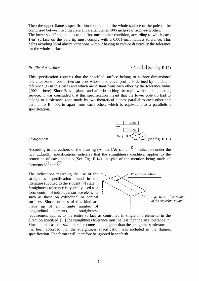
Straightness (see fig. II.13)

According to the authors of the drawing (Annex [A6]), the " " indication under the

two specifications indicates that the straightness condition applies to the

centerline of each pole tip (See Fig. II.14), in spite of the mention being made of

elements and .

The indications regarding the use of the

straightness specification found in the

literature supplied to the student [4] state: "

Straightness tolerance is typically used as a

form control of individual surface elements

such as those on cylindrical or conical

surfaces. Since surfaces of this kind are

made up of an infinite number of

longitudinal elements, a straightness

requirement applies to the entire surface as controlled in single line elements in the

direction specified. [...]The straightness tolerance must be less than the size tolerance. "

Since in this case the size tolerance comes to be tighter than the straightness tolerance, it

has been accorded that the straightness specification was included in the flatness

specification. The former will therefore be ignored henceforth.

Pole tip centerline

Fig. II.14: Illustration

of the centerline notion

15

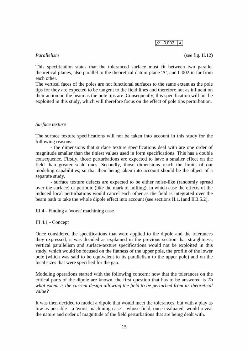
Parallelism (see fig. II.12)

This specification states that the toleranced surface must fit between two parallel

theoretical planes, also parallel to the theoretical datum plane 'A', and 0.002 in far from

each other.

The vertical faces of the poles are not functional surfaces to the same extent as the pole

tips for they are expected to be tangent to the field lines and therefore not as influent on

their action on the beam as the pole tips are. Consequently, this specification will not be

exploited in this study, which will therefore focus on the effect of pole tips perturbation.

Surface texture

The surface texture specifications will not be taken into account in this study for the

following reasons:

- the dimensions that surface texture specifications deal with are one order of

magnitude smaller than the tiniest values used in form specifications. This has a double

consequence. Firstly, those perturbations are expected to have a smaller effect on the

field than greater scale ones. Secondly, those dimensions reach the limits of our

modeling capabilities, so that their being taken into account should be the object of a

separate study.

- surface texture defects are expected to be either noise-like (randomly spread

over the surface) or periodic (like the mark of milling), in which case the effects of the

induced local perturbations would cancel each other as the field is integrated over the

beam path to take the whole dipole effect into account (see sections II.1.1and II.3.5.2).

IIIIII..44 -- FFiinnddiinngg aa ''wwoorrsstt'' mmaacchhiinniinngg ccaassee

III.4.1 - Concept

Once considered the specifications that were applied to the dipole and the tolerances

they expressed, it was decided as explained in the previous section that straightness,

vertical parallelism and surface-texture specifications would not be exploited in this

study, which would be focused on the flatness of the upper pole, the profile of the lower

pole (which was said to be equivalent to its parallelism to the upper pole) and on the

local sizes that were specified for the gap.

Modeling operations started with the following concern: now that the tolerances on the

critical parts of the dipole are known, the first question that has to be answered is To

what extent is the current design allowing the field to be perturbed from its theoretical

value?

It was then decided to model a dipole that would meet the tolerances, but with a play as

low as possible - a 'worst machining case' - whose field, once evaluated, would reveal

the nature and order of magnitude of the field perturbations that are being dealt with.

16

The present section presents the model that was adopted for that function, after a phase

of experimentation on modeling possibilities and limitation, along with the perturbation

that were applied to it.

III.4.2 - Presentation of the model

Figure II.15 shows an overview of the geometry of the

'ABH' model, realized in the Opera modeler according to

the design specifications for the 'AB' magnet and for its

steel extension.

Since the perturbation applied to the pole tips are of the

order of magnitude of the tolerances that were applied to

those surfaces (i.e. ~10-3

in), they are not visible on an

overview of the magnet.

Specific steel magnetic properties were specified (Fig.

II.16) for the behavior of the modeled steel to be as close as

possible to the steel that is actually used to build the

CEBAF magnets.

Fig. II.15: Overview of

the first perturbed

model of the ABH

magnet

Fig. II.16: B-H curve defining the properties of the steel used in the

calculations, obtained from measurements on steel taken on a section of steel

from an ingot used in making CEBAF magnets.

17

III.4.3 - Perturbations applied

This paragraph deals with the perturbations that were chosen to be applied in this

model.

Transverse perturbations

Let us consider a transverse plane, perpendicular to the general beam direction, in order

to discuss the nature, extent and justification of the perturbations that are perceivable

transversally.

Figure II.17 gives a schematic representation of the shape of the perturbed pole tips in a

transverse plane.

Since the parallelism tolerance ( ) is a relative property, it was decided that the

reference 'B' on the upper pole was going to be modeled horizontally for the parallelism

defect to be easily managed by the orientation of the lower pole.

This election implies that the upper pole has a transverse flatness default of 0.002

inches, which is the maximum tolerated since:

- it is only 4 inches wide,

- the flatness default cannot exceed 0.001 in per inch,

- the tangent plane has to be horizontal for the flatness and parallelism defects to

be treated separately.

The upper pole flatness defect was at that stage modeled by a parabola, since it was

assumed that this convex shape would favor the divergence of the field lines on the

sides of the poles, thus magnifying the effect of the tip non-planarity on the field.

Fig. II.17: Schematic representation of the

pole tips' perturbed shape

xy08.5

00254.0

241007996850393701 x.y

Equations of the slope and parabola:

18

The parallelism specification that was applied to the lower pole by means of the profile

specification ( ) was taken into account by 'tilting' the lower pole tip with a

precisely defined slope so that its tip can be exactly 0.002 inches non-parallel to the

upper pole's 'B' reference datum plane: a tangent plane that was made horizontal on

purpose, as explained before.

In that configuration, one can verify that the local size specification is verified

everywhere.

Longitudinal perturbations

In a first step, it was decided that longitudinal perturbations would not be taken into

account, for modeling reasons. In fact, the vertical symmetry of the model was broken

by the introduction of the transverse perturbations, which caused the model size, and the

calculation time thus, to almost double. Introducing longitudinal perturbations would

break the longitudinal symmetry, doubling the solver burden once more. Since

perturbed models took around 15 hours to solve, it was decided that the study would

start with transversal perturbations only.

From another point of view, the longitudinal axis is parallel to the machining direction,

so that most of its defect content is likely to be related with vertical milling marks,

which was said to be negligible in the surface texture paragraph of the II.3.3.2 section

on tolerances.

In the end, longitudinal perturbations are not treated in this study.

IIIIII..55 -- FFiieelldd eevvaalluuaattiioonn mmeetthhoodd

III.5.1 - Definition of multipoles

Introduction

When an accelerator is constructed, the nominal trajectory of the particle beam is fixed.

This trajectory may simply be a straight line, as is the case in linear accelerators. In

circular machines such as the CEBAF in its entirety, however, it has a more complicated

shape consisting of numerous curves connected by straight sections of various length

(the spreaders are a good example of that complexity). The beam follows the resulting

path until it is accelerated to the required extent and is sent to the halls. But on another

scale, the trajectories of individual particles within the beam always have a certain

angular divergence and without further measures the particles would eventually hit the

wall of the vacuum chamber and be lost.

It is therefore necessary first of all to fix the beam trajectory, in general an arbitrary

curve and then to repeatedly steer the diverging particles back onto the ideal trajectory.

The latter, termed the 'orbit', is fixed by the construction of the accelerator, taking

numerous parameters into account, such as the energy of the particles, a reasonable

steering radius for them given the field strength that can be reached by the magnets and

the desired/available size for the accelerator facility... In most general terms, the

steering is done by means of electromagnetic fields ( E

and B

) in which particles of

charge e and velocity v

v experience the Lorentz force:

(2) )( BvEeF

19

At relativistic velocities, the effect of magnetic fields is so strong compared to the effect

of technically achievable electric fields that those are mostly employed at very low

energies.

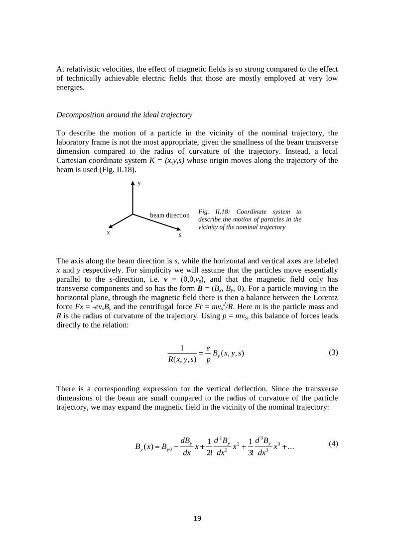
Decomposition around the ideal trajectory

To describe the motion of a particle in the vicinity of the nominal trajectory, the

laboratory frame is not the most appropriate, given the smallness of the beam transverse

dimension compared to the radius of curvature of the trajectory. Instead, a local

Cartesian coordinate system K = (x,y,s) whose origin moves along the trajectory of the

beam is used (Fig. II.18).

The axis along the beam direction is s, while the horizontal and vertical axes are labeled

x and y respectively. For simplicity we will assume that the particles move essentially

parallel to the s-direction, i.e. v = (0,0,vs), and that the magnetic field only has

transverse components and so has the form B = (Bx, By, 0). For a particle moving in the

horizontal plane, through the magnetic field there is then a balance between the Lorentz

force Fx = -evsBy and the centrifugal force Fr = mvs2/R. Here m is the particle mass and

R is the radius of curvature of the trajectory. Using p = mvs, this balance of forces leads

directly to the relation:

(3)

There is a corresponding expression for the vertical deflection. Since the transverse

dimensions of the beam are small compared to the radius of curvature of the particle

trajectory, we may expand the magnetic field in the vicinity of the nominal trajectory:

(4)

beam direction

y

s x

Fig. II.18: Coordinate system to

describe the motion of particles in the

vicinity of the nominal trajectory

...!3

1

!2

1)( 3

3

3

2

2

2

0 xdx

Bdx

dx

Bdx

dx

dBBxB

yyy

yy

),,(),,(

1syxB

p

e

syxRy

20

Multiplying by e/p:

The magnetic field around the beam may therefore be regarded as a sum of terms, called

multipoles, each of which has a different effect on the path of the particles.

Interpretation

The notion of multipoles is of fundamental importance in order to understand the results

of the present study, since most of its conclusions will deal with the extent of a

multipole's contribution in the field. This notion has a variety of interpretations, and one

should not simply stick to the representation in terms of a mathematical expansion.

From this perspective, one should however keep in mind two concepts:

- the behavior of the field components with respect to the distance from the ideal

beam trajectory, which is a constant for the dipole, a linear slope for the quadrupole, a

square dependence for the sextupole...

- the linear nature of a sum which confers intrinsic independence to the different

components of the magnetic field

The different names that are given to the terms of the expansion clearly come from the

homonym magnets. In the case of a dipole magnet like the ABH for example, the field

lines are straight and parallel between the poles (disregarding edge effects) which means

that their density - the magnetic flux density 'B' - is constant, as the dipole term in the

expansion was. In a quadrupole magnet, the field lines have the shape indicated in

figure II.19. One sees that they get closer and closer to each other as the distance from

the center raises, and this density growth is actually linear, as was seen in the

'quadrupole' term of the mathematical expansion of the field.

... !3

1

!2

1

1

...!3

1

!2

1)(

32

3

3

3

2

2

2

0

oxmxkxR

xdx

Bd

p

ex

dx

Bd

p

ex

dx

dB

p

eB

p

exB

p

e yyy

yy

Dipole Quadrupole Sextupole Octupole

Fig. II.19: Shape of the field

lines in a quadrupole magnet

21

Fig. II.20: Illustration of the field

measurement using a rotating coil

This correspondence between mathematical and physical tools is the basic concept that

enables accelerator physicists to build the lattice, the sequence of magnets which

constitutes the accelerator along with their set points, so that each mathematical

component of the field seen by the particles along the beam path can be managed with a

real and concrete magnet type.

III.5.2 - Measuring multipoles

Introduction

As was mentioned in the previous section, the field multipoles have a relatively wide set

of interpretation perspectives. In order to understand the way they are measured, treated

and compared in this study it is necessary to get acquainted with the cylindrical

representation of multipoles.

The mathematical expansion presented in section II.3.5.1 was expressed in a Cartesian

coordinate system and the distance from the nominal trajectory was expressed in terms

of the abscissa along the horizontal axis x. However, the smallness of the beam

transverse dimensions compared to the radius of curvature of the trajectory is respected

in every direction normal to the trajectory, which confers to the system a cylindrical

complexion that is better described in polar coordinates.

The measurement and diagnosis of multipoles underwent

somewhat of a revolution around 1965 when J. Cobb and

R. Cole used a fast rotating coil to measure quadrupoles at

SLAC (Stanford Linear Accelerator Center) in California

[5]. The idea is based on the description of magnetic

fields in terms of their Fourier harmonic expansion.

Picture a coil (Fig. II.20) rotating with constant angular

velocity. One side of the coil is placed colinear with the

axis of the magnet, the other side sweeps out a circle of

constant radius. The voltage seen on an oscilloscope is

proportional to the rate of flux cut by the coil. If the

magnet is perfect, a perfect sine or cosine wave should be

seen at a frequency equal to the revolution frequency for a

dipole, twice the revolution frequency for a quadrupole, etc.

The field expansion in cylindrical coordinates is generally expressed:

(5)

(6)

1

1 )sin(),(n

n

n

nr nrKrB

1

1 )cos('),(n

n

n

n nrKrB

22

With the following correspondence:

Field evaluation in simulations

The numerical code used in this study [1] to model the dipoles and compute their field

has a feature that allows to measure the quality of the field induced by modeled magnets

in a way that is very similar to the rotating coil technique, so that it is possible to

compare the results of calculations with measured data when available.

In the real measurements that are made at Jlab, the coil is rotated around the beam path

as described in the previous paragraph and then moved longitudinally to measure the

field along the beam trajectory. As the quantity measured is the amount of flux cut by

the coil, all the harmonics are summed and cannot be measured independently. More

advanced devices are able to separate the harmonics via a set of multiple dedicated

coils.

In the simulated models, the field is evaluated along a circle in a plane normal to the

beam trajectory (Fig. II.21). The circle is then displaced along a trajectory that follows

the expected beam path - e.g. a circular path within the bending dipole field - and the

field is evaluated at each step. A Fourier fit is computed from the circular field

evaluation along each circle, simulating the values that would be measured for the field

multipoles using rotating coils in a real magnet.

n = 1 Dipole

n = 2 Quadrupole

n = 3 Sextupole

n = 4 Octupole

n = 5 Decapole

n = 6 Dodecapole or 12 pole

Fig. II.21: Representation of the 1-cm circle around

which the fields are evaluated in the simulated models

23

The script used to generate the circles along the beam path can be found in annex [A3].

The file that is being presented has been shortened for paper economy reasons and only

presents the first 5 cm and the last 5 cm of the 75cm-long defined trajectory.

The actual coordinates of the points defining the circles as well as the harmonic values

from the Fourier fit applied to the fields evaluated on the circles are given in annex

[A1].

As mentioned in section II.3.1.1 - Software resources, the format in which the

harmonics are presented in the post processor output file [A1] is quite incompatible with

the syntax required for treatment with a spreadsheet editor such as those used in this

study [2] [3]. A Perl script, given in annex [A2], was therefore edited by the student to

generate a double-entry array presenting the value of each harmonic on each circle all

along the beam path.

The circles used to evaluate the 'ABH' magnet models have a radius of 1 cm. This value

has been decided upon according to several criteria:

1) The radius cannot be much larger for the magnet poles are only 1.295 cm

away from the beam trajectory (and thus from the center of the circle) and a circle

evaluating fields too close to the poles would see its evaluation accuracy reduced due to

irregularities in the mesh inherent to a change of medium.

2) Since the fields around the circle are evaluated by nodal interpolation, the

perimeter of the circle has to be sufficient for the number of finite elements available for

the interpolation along the circle to satisfy the sampling theorem.

The Nyquist-Shannon sampling theorem states that:

"If a function f(t) contains no frequencies higher than W cps*, it is completely

determined by giving its ordinates at a series of points spaced 1/(2W) seconds apart."

*: Cycles per second - modern unit is Hertz (Hz)

Here the application of this theorem is geometrical instead of temporal: since we are

evaluating cyclic functions around a circle, W won't be expressed in terms of cycles per

second but in terms of cycles per perimeter of the circle. Since the multipoles are

evaluated up to the 20-pole (which is then the one with higher frequency), W here is 10

cycles per perimeter. For a 1-cm radius circle, the perimeter length is about 63 mm.

Therefore, the field has to be evaluated at least every each 1/(2W)*63 mm = 3.15 mm.

Since in the models studied the mesh size is 2.5 mm in the gap, the sampling theorem is

verified with a 1-cm radius circle.

3) Equations (5) and (6) show that each 2n-pole term is proportional to rn-1

so

that even evaluations made with a large circle can eventually lead to an evaluation at a

beam-radius scale.

24

III.5.3 - On skew multipoles

Before the research proceeding goes on with the presentation of the first results in the

next section, a few precisions about field multipoles should be considered in order to

clearly understand those results.

We have seen in the previous section that the field induced by a perfect 2n-pole magnet

could be described as a theoretical say, cosine wave. Basic notions of trigonometry tell

us that a rotation of π/2n of the coordinate system implies that a term be expressed with

a sine if it had a cosine and vice versa. This has a very important repercussion on the

practical field for it implies that the field of a perfect 2n-pole magnet can be described

by, say, a sine wave in only one coordinate system or in other words, that in a given

coordinate system, we generally need both sine term and cosine term to describe the

field content at any given order n because of the angular degree of freedom around the

longitudinal axis.

In reality, magnets are never perfectly vertical or perfectly horizontal. There is always a

component of the field that is not aligned with the reference, intrinsic to the magnet mis-

orientation. Moreover, as the fields induced by the magnets are never quite perfect, even

in their own coordinate system, the terms representing 'tilted' content - which are called

the skew terms - help the accelerator scientists to describe unwanted components of the

magnetic field.

Fig. II.22: Field evaluation around a 1-cm radius circle situated in the center

of an unperturbed model of the 'ABH' Dipole. One can clearly see the

cosinusoidal shape that was mentioned in the introduction of this section.

25

IIVV -- RReessuullttss

IIVV..11 -- EEffffeecctt ooff tthhee iinnttrroodduuccttiioonn ooff aa ppeerrttuurrbbaattiioonn

The goal of this section is to obtain a first look at the effect that the introduction of a

geometrical perturbation in the numerical model of the studied dipole has on its field.

For this purpose, the 'Worst Machining Case' (WMC) model, defined in section II.3.4,

will first be compared to the original, non-perturbed model that is currently being used

to simulate the 'ABH' magnet in the accelerator simulations (cf. II.1.1).

IV.1.1 - Presentation of the original model

From now on, the models will be described in a coordinate system in which the origin is

placed in the center of the gap (equal distance from the pole tips and from their

borders), z is the longitudinal axis and x and y the transverse directions respectively

parallel and normal to the pole tips.

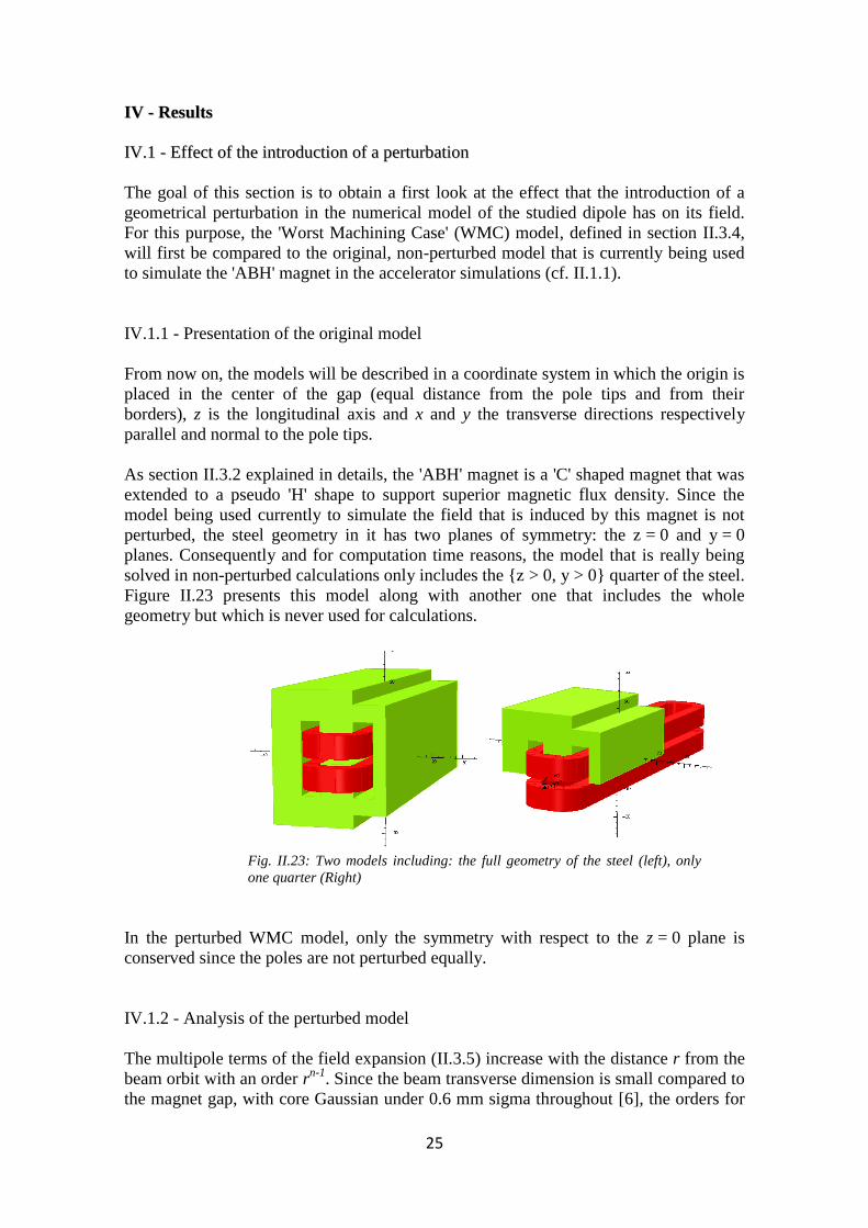
As section II.3.2 explained in details, the 'ABH' magnet is a 'C' shaped magnet that was

extended to a pseudo 'H' shape to support superior magnetic flux density. Since the

model being used currently to simulate the field that is induced by this magnet is not

perturbed, the steel geometry in it has two planes of symmetry: the z = 0 and y = 0

planes. Consequently and for computation time reasons, the model that is really being

solved in non-perturbed calculations only includes the {z > 0, y > 0} quarter of the steel.

Figure II.23 presents this model along with another one that includes the whole

geometry but which is never used for calculations.

In the perturbed WMC model, only the symmetry with respect to the z = 0 plane is

conserved since the poles are not perturbed equally.

IV.1.2 - Analysis of the perturbed model

The multipole terms of the field expansion (II.3.5) increase with the distance r from the

beam orbit with an order rn-1

. Since the beam transverse dimension is small compared to

the magnet gap, with core Gaussian under 0.6 mm sigma throughout [6], the orders for

Fig. II.23: Two models including: the full geometry of the steel (left), only

one quarter (Right)

26

n > 2 will be neglected for now in front of the two first terms. Since the dipole skew

term is null and its normal (not skew) term is easily taken into account in real

measurements given its direct effect on the beam trajectory, only the quadrupole term is

going to be taken into account at first.

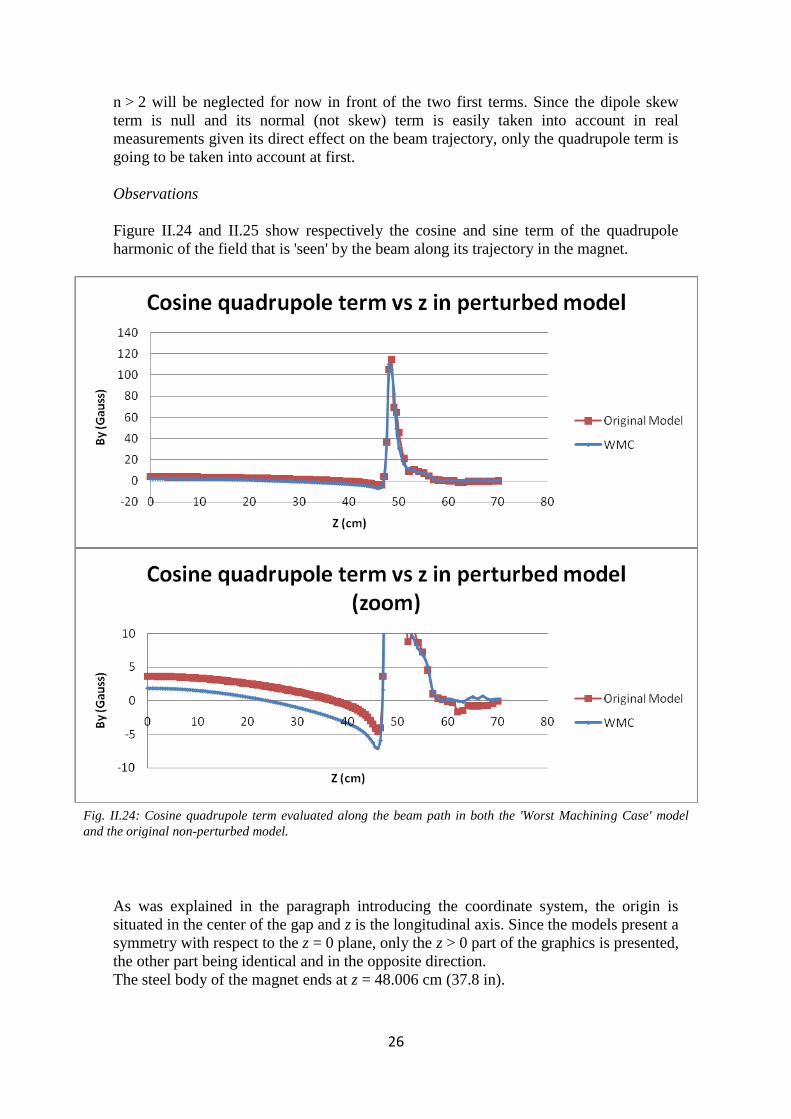
Observations

Figure II.24 and II.25 show respectively the cosine and sine term of the quadrupole

harmonic of the field that is 'seen' by the beam along its trajectory in the magnet.

As was explained in the paragraph introducing the coordinate system, the origin is

situated in the center of the gap and z is the longitudinal axis. Since the models present a

symmetry with respect to the z = 0 plane, only the z > 0 part of the graphics is presented,

the other part being identical and in the opposite direction.

The steel body of the magnet ends at z = 48.006 cm (37.8 in).

Fig. II.24: Cosine quadrupole term evaluated along the beam path in both the 'Worst Machining Case' model

and the original non-perturbed model.

27

One can see a slight offset in the cosine term value while the beam is still between the

poles, but since the tendency is not modified and the lattice is equipped with numerous

normal 'cosine oriented' quadrupole magnets, this effect is easy enough to correct for

this study not to focus on it.

Several interesting phenomena are observed here. While the non-perturbed model had

all its skew terms artificially set to 0 for the magnet mid-plane (y = 0) was a boundary

for the model (and thus the boundary condition stated that the field lines had to be

normal to the mid-plane), the perturbed model, in which this symmetry is broken,

shows:

- a constant body term of several Gauss

- a peak at the end of the steel, one order of magnitude higher than the body

value

Fig. II.25: Sine quadrupole term evaluated along the beam path in both the WMC model and the original non-

perturbed model

28

Comments

As was explained before, the lattice is supplied with numerous normal quadrupole

magnets, so that the normal quadrupole perturbation is not much of a problem for it can

be corrected easily. On the other hand, skew quadrupole magnets are rare and most of

them are situated in the linacs, already set to compensate for the skew terms introduced

by the imperfect superconducting RF cavities. There are only two skew quadrupoles in

the CEBAF outside the linacs, in the eighth and ninth spreaders. These are used to

compensate for all the accumulated error outside the linacs, which represents an

equivalent of over 600 cumulated meters of dipole length before the ninth spreader.

They are set to reduce x-y coupling to the part per thousand level in the succeeding arc.

Typical values are 500-800 G - which is roughly equivalent to 1 Gauss per meter of

dipole. Dipole values are about 40% of those considered in this work (see section

II.4.2), so 2.5 G per meter of dipole would be typical in the upgrade if disassembling the

dipoles to modify the coils and reassembling with H steel do not alter performance.

First normal multipoles are useful: dipoles are used to steer the beam, and quadrupoles

to focus it for example. But skew multipole terms play an important role in beam

deterioration throughout the accelerator. At 6 GeV the distribution of the particles in the

beam transverse dimension is Gaussian and the beam diameter is easily kept under

0.2mm sigma (core Gaussian) [6] throughout. Halo with a quadratic (not Gaussian)

transverse profile is sometimes introduced accidentally in the injector and interacts with

higher multipoles throughout the machine. As the energy raises (the upgrade purpose is

to double it), the synchrotron radiation becomes significant in the arcs and to the initial

distribution is added a halo even without injector error. Again, this halo is a

quadratically-distributed noise zone around the Gaussian that increases the beam

transverse dimension. As was seen many times before, multipole terms get higher with

the distance from the center of the beam and as the beam transverse dimension

increases, so does its sensitivity to multipole effects. Beam section increase and

sensitivity to skew multipole content are two parasite phenomena which favor each

other.

Since there are hundreds of dipoles in the lattice, their introducing a hitherto neglected

skew term must be studied in details.

Proposal

At this point of the study, it appears clearly that modeling the magnets using only a

quarter of the steel for symmetry reasons was too bold an assumption. However, we

don't know yet to what extent the skew terms observed in the perturbed model are due

to full-height steel modeling or to the actual perturbation.

The next step should therefore be to compare our perturbed model to an unperturbed

model comprising the full height of the steel, thus getting rid of the boundary condition

that zeroed all skew content of the field in the previous simulation.

29

IV.1.3 - Comparison with a full-height, non-perturbed model

Figure II.26 shows how the full height of the steel is comprised in the non-perturbed

model that is going to be used henceforth, while the longitudinal symmetry that allows

us to keep calculation time reasonable is still conserved. Quarter-steel models took

roughly half the time half-steel models take to solve, which means that the calculation

time passed from around 6-7 hours to around 15 hours. One should keep in mind that

each of the simulations presented in this study is the result of several hours of modeling

and meshing in the case of perturbed models, plus one night of calculation on a general

basis.

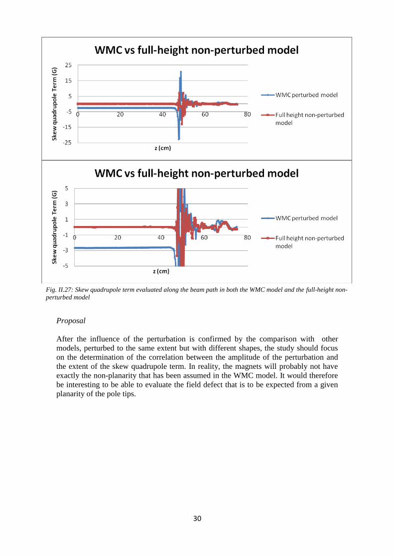
One can observe on figure II.27 that:

- the ~3 Gauss shift in the zone between the poles is conserved

- the unperturbed model now shows a bunch of peaks in the pole edge

whereabouts

Interpretation

Although the end of the pole tips are likely to have an influence on the field, the high

frequency peak shape that is observed is very unlikely to have any physical relevance.

These oscillations are more probably caused by the insufficient mesh density outside the

gap zone. While the finite element size is 2.5 mm in the gap, it changes to 5 mm when

the beam gets out of the magnet. Although this edge effect is interesting, the study will

first focus on the body field whose calculation is more reliable for now (cf. II.3.5.2).

Fig. II.26: 3D representation of the two unperturbed models, respectively assuming a double symmetry

(left), or only one longitudinal symmetry (right).

30

Proposal

After the influence of the perturbation is confirmed by the comparison with other

models, perturbed to the same extent but with different shapes, the study should focus

on the determination of the correlation between the amplitude of the perturbation and

the extent of the skew quadrupole term. In reality, the magnets will probably not have

exactly the non-planarity that has been assumed in the WMC model. It would therefore

be interesting to be able to evaluate the field defect that is to be expected from a given

planarity of the pole tips.

Fig. II.27: Skew quadrupole term evaluated along the beam path in both the WMC model and the full-height non-

perturbed model

31

IV.1.4 - Comparison with other perturbed models

Presentation of the other perturbed models

Figure II.28 presents the shapes that were used to perturb the Test1 and Test2 models.

They were mostly chosen to test asymmetric and non-linear shapes, without taking into

account their being realistic or not for the moment.

Fig. II.28: Presentation of the two

additional perturbed models that

were used to verify the apparition

of a skew term in the zone between

the poles.

Original Model : Parallel planar poles Test1 : Parabolic convex upper pole, cosinusoidal lower pole Test2 : Parabolic convex upper pole, sinusoidal lower pole (1/2 period) WMC : Parabolic convex upper pole, tilted planar lower pole

Test2

Test1

32

Observations

Figure II.29 shows that a skew term is observed in each model and that they all have

very similar values, although the sign is opposed in Test1.

Conclusions

It is now confirmed that the geometrical perturbation of the poles creates a skew

quadrupole term in the gap of the dipoles. Its sign seems to be related to the relative

symmetry of the perturbations.

The arguments that led to decide upon a convex parabola and a tilt for the WMC model

were more mathematical than practical:

- the convex shape was assumed to favor the divergence of the field lines

- the tilt was intended to introduce asymmetry and it represented the non-

parallelism of the poles.

Although the pole tips are indeed very likely to be somewhat non-parallel in reality, the

convex shapes that those models present are very unrealistic on the contrary.

When a surface is milled vertically, the two main causes for shape defects are the

orientation of your mill and the quality of the guiding. Since the latter only has a

longitudinal effect that is not taken into account in the present study, let us focus on the

former:

- if the mill is tilted with respect to the longitudinal axis, the machined surface,

as planar as it may be, will end up being tilted by the same amount

- if the mill is tilted with respect to the transverse axis, the machined surface will

be a concave ellipse instead of a plane

Fig. II.29: Skew Quad term over the length of the pole tips for the

full-height perfect model and for three different perturbed models.

33

Since the apparition of a tilt or an ellipse instead of a plane is independent from the sign

of the mill orientation defect, one can conclude that those form defects are always going

to be present on the pole tips, to some extent.

Proposal

Now that the influence of geometrical perturbations has been qualitatively established,

the next step in the research progress will be to determine quantitatively the correlation

between the amplitude of the geometrical perturbation and the amplitude of the induced

field perturbation.

A model presenting a concave ellipse and a tilt should be used for this purpose.

IIVV..22 -- EEffffeecctt ooff FFiieelldd IInntteennssiittyy

Before the research process goes on with the quantitative study of the influence of

geometrical perturbations on the field, a parallel study whose purpose is to verify an

initial assumption will be presented.

Initial assumption

As section II.3.2.3 stated, the 'ABH' magnet was chosen for this study because it was

going to induce the strongest dipole field in the 12GeV-set lattice (~14kG). It was

assumed that the steel saturation occurring at those fields would favor field defects and

make the study more easily readable.

Verification process

To verify this assumption, it was decided that the initial perturbed model would be

solved using different current densities in order to see the tendency of the field

perturbation with respect to steel saturation. Since the magnet is never going to be used

with higher current than its 12-GeV nominal current I, it was decided that the model

would be solved for the following values of the current: .25I, .375I, .5I, .625I, .75I,

.875I, I (already solved).

Figure II.30 presents the results of these calculations. A unique value that would

represent accurately the field in the gap of each model was needed. Since the previous

section showed that the quadrupole term of the field was rather constant far from the

edges, an average of the skew quadrupole term of the field was computed for each

model over the z = 0 to z = 20 cm portion of the beam trajectory.

With an average around 15 h of calculation time for each model, solving them all took a

little more than 100 h.

34

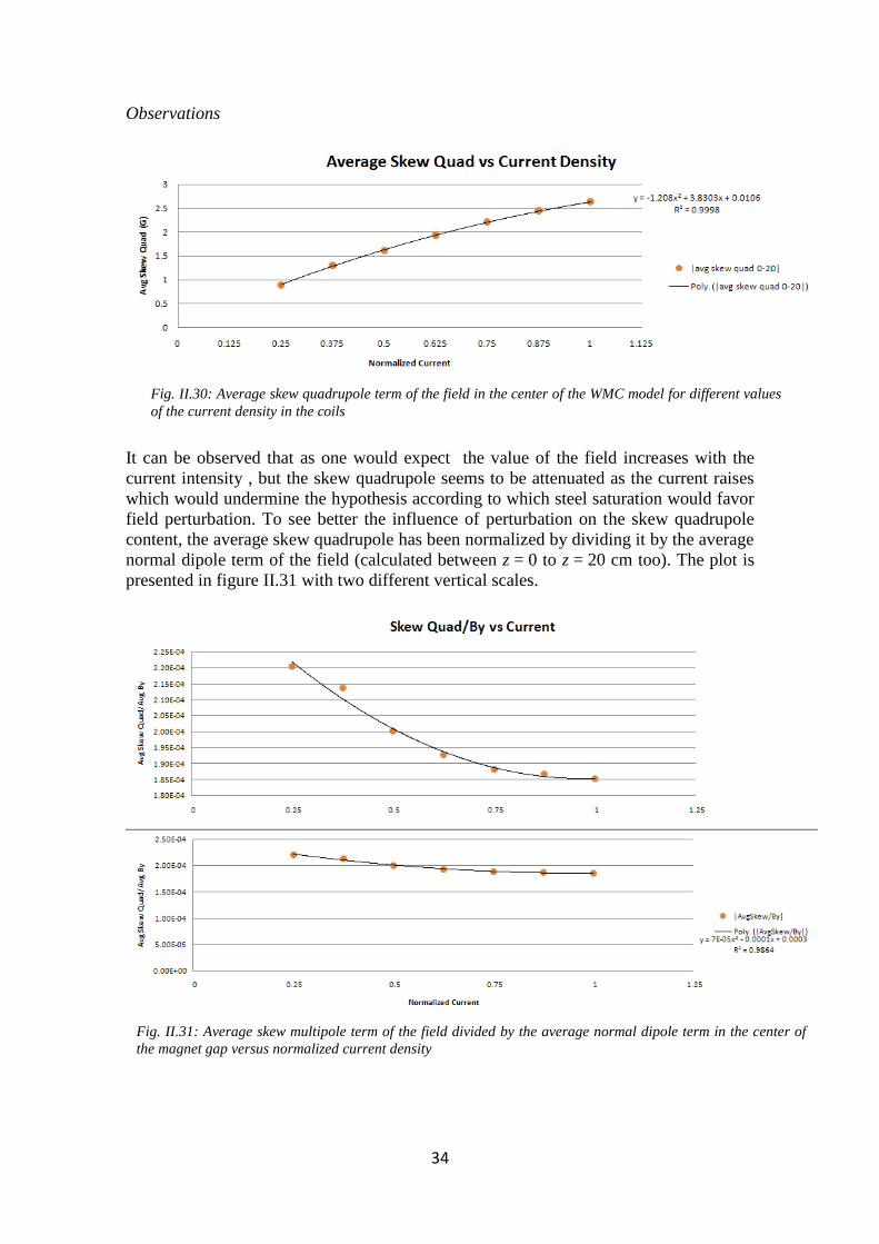
Observations

It can be observed that as one would expect the value of the field increases with the

current intensity , but the skew quadrupole seems to be attenuated as the current raises

which would undermine the hypothesis according to which steel saturation would favor

field perturbation. To see better the influence of perturbation on the skew quadrupole

content, the average skew quadrupole has been normalized by dividing it by the average

normal dipole term of the field (calculated between z = 0 to z = 20 cm too). The plot is

presented in figure II.31 with two different vertical scales.

Fig. II.31: Average skew multipole term of the field divided by the average normal dipole term in the center of

the magnet gap versus normalized current density

Fig. II.30: Average skew quadrupole term of the field in the center of the WMC model for different values

of the current density in the coils

35

One can see clearly that the relative importance of the skew multipole term with respect

to the functional steering field decreases as saturation raises.

Interpretation

This decrease of the relative importance of the skew multipole means that as the magnet

is used with higher and higher currents, it becomes relatively less sensitive to the

geometrical defects of its poles.

This can be interpreted considering the nature of the saturation phenomenon. As the

current augments in the coils, the magnetic field induced in the steel grows. This means

that the magnetic flux density increases, that the density of field lines guided by the

steel increases. When the steel starts to saturate, its permeability decreases and it admits

less and less additional field lines. Since the flux generated by the coils raises anyway,

the field lines start to be driven by the air instead of being sucked by the steel. The

magnet starts to be less and less 'iron-dominated'.

As the air drives more and more flux compared to the steel, its influence on the field

shape gets more and more important. Since geometrical perturbations of the pole tips

only affect the field lines that are driven by the steel, one can understand the decrease of

their relative influence with the decrease of the relative influence of the steel on the

field shape.

Conclusion

The initial assumption regarding the help that steel saturation would provide in studying

the influence of geometrical perturbations was wrong, as its effect is actually to lower

their influence. However, since this effect is limited to ~20% of the studied value (Fig.

II.31) and since this saturation influence verification was being undertaken in parallel to

the rest of the perturbation studies, it was decided that the studies should keep using the

ABH magnet. One can later translate the results to weaker magnets using the established

curves.

36

IIVV..33 -- QQuuaannttiittaattiivvee iinnfflluueennccee ooff ggeeoommeettrriiccaall ppeerrttuurrbbaattiioonnss

The purpose of this section will be to look for an exploitable correlation between the

amplitude of the geometrical perturbations and their expected effect on the field

components.

IV.3.1 - Models used

Presentation

As section II.4.1 explained the convex shapes that have been used to model the

perturbations until now are not realistic. As a consequence, the models that are going to

be used from now on will have perturbations whose shape can logically be expected

from machining defects. It was established that, to some extent, any milled surface is

tilted and presents a concave elliptic shape. This is therefore the way in which

perturbations will be modeled. However, and although each pole tip should present both

a tilt and an concave elliptic shape, those defects will be separated in order to be able to

quantify their amount more clearly. This separation will be done artificially by using

models that present a concave elliptic upper pole, and a planar tilted lower pole.

The first model created that way was intended to be an equivalent of the WMC model in

the way that it was modeled to fulfill the tolerances with a play as low as possible.

Nevertheless, since the objective was not to match the tolerances anymore but to make a

model that could be easily modified to study different values for the perturbation, this

model was dimensioned with metric units, having a perturbation amplitude of 50

microns, versus 0.002 in for the WMC model. The 0.002 in value came from the

drawings edited by the engineers, who use the U.S. customary unit system on a general

basis, and the 50 microns value was intended to be a starting point for a set of

simulations with different perturbation amplitudes that would be realized in a metric

system scientific environment (numerical codes, internal communication...).

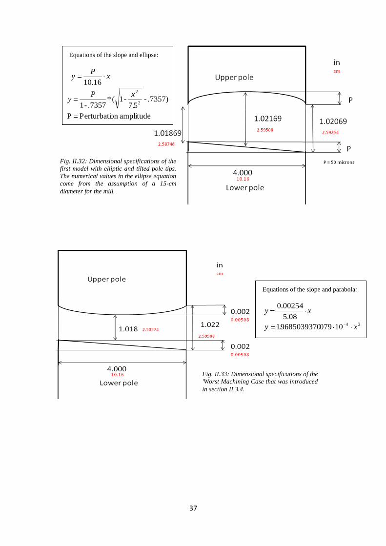
Figures II.32 and II.33 respectively present the new elliptic and tilted model and the

WMC model, for comparison.

37

Fig. II.33: Dimensional specifications of the

'Worst Machining Case that was introduced

in section II.3.4.

xy08.5

00254.0

241007996850393701 x.y

Equations of the slope and parabola:

Fig. II.32: Dimensional specifications of the

first model with elliptic and tilted pole tips.

The numerical values in the ellipse equation

come from the assumption of a 15-cm

diameter for the mill.

xP

y16.10

Equations of the slope and ellipse:

amplitudeon Perturbati P

.7357)-57

-1(*.7357-1 2

2

.

xPy

38

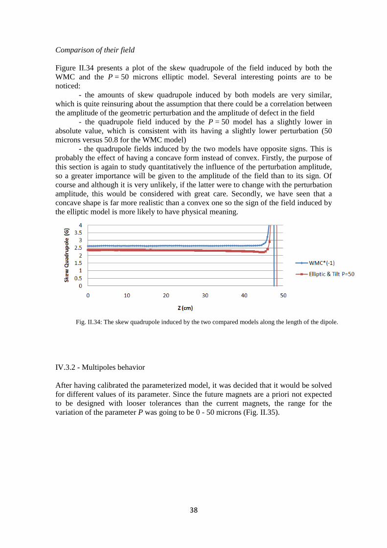
Comparison of their field

Figure II.34 presents a plot of the skew quadrupole of the field induced by both the

WMC and the P = 50 microns elliptic model. Several interesting points are to be

noticed:

- the amounts of skew quadrupole induced by both models are very similar,

which is quite reinsuring about the assumption that there could be a correlation between

the amplitude of the geometric perturbation and the amplitude of defect in the field

- the quadrupole field induced by the P = 50 model has a slightly lower in

absolute value, which is consistent with its having a slightly lower perturbation (50

microns versus 50.8 for the WMC model)

- the quadrupole fields induced by the two models have opposite signs. This is

probably the effect of having a concave form instead of convex. Firstly, the purpose of

this section is again to study quantitatively the influence of the perturbation amplitude,

so a greater importance will be given to the amplitude of the field than to its sign. Of

course and although it is very unlikely, if the latter were to change with the perturbation

amplitude, this would be considered with great care. Secondly, we have seen that a

concave shape is far more realistic than a convex one so the sign of the field induced by

the elliptic model is more likely to have physical meaning.

IV.3.2 - Multipoles behavior

After having calibrated the parameterized model, it was decided that it would be solved

for different values of its parameter. Since the future magnets are a priori not expected

to be designed with looser tolerances than the current magnets, the range for the

variation of the parameter P was going to be 0 - 50 microns (Fig. II.35).

Fig. II.34: The skew quadrupole induced by the two compared models along the length of the dipole.

39

One can observe that the value of the quadrupole field increases with the value of the

geometrical perturbation which confirms a dependence. The next step is to determine

the character of this dependence. To be able to plot the intensity of the field induced by

the modeled magnets in function of their perturbation parameter, one needs a value that

would represent the extent of the multipole content of the field for a given magnet. The

integrated field along the beam path is widely used for that purpose. This integral:

(7)

can be calculated for each multipole harmonic of the field independently, by linear

property of the integral. In this case it is calculated numerically (with a finite step) using

the table of evaluated fields generated by the script which evaluates the multipoles

(II.3.5.2) [A3]. Each integral is however normalized by dividing the multipole value by

Fig. II.35: Skew quadrupole field induced by the perturbed

models for P = 0, 5, 10, 17, 25 and 50 microns

beampath

ldB

.

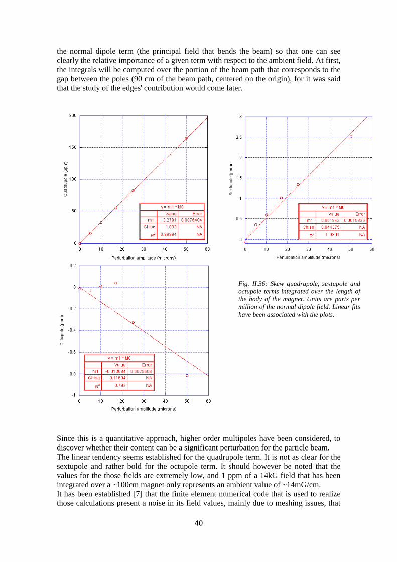
40

the normal dipole term (the principal field that bends the beam) so that one can see

clearly the relative importance of a given term with respect to the ambient field. At first,

the integrals will be computed over the portion of the beam path that corresponds to the

gap between the poles (90 cm of the beam path, centered on the origin), for it was said

that the study of the edges' contribution would come later.

Since this is a quantitative approach, higher order multipoles have been considered, to

discover whether their content can be a significant perturbation for the particle beam.

The linear tendency seems established for the quadrupole term. It is not as clear for the

sextupole and rather bold for the octupole term. It should however be noted that the

values for the those fields are extremely low, and 1 ppm of a 14kG field that has been

integrated over a ~100cm magnet only represents an ambient value of ~14mG/cm.

It has been established [7] that the finite element numerical code that is used to realize

those calculations present a noise in its field values, mainly due to meshing issues, that

Fig. II.36: Skew quadrupole, sextupole and

octupole terms integrated over the length of

the body of the magnet. Units are parts per

million of the normal dipole field. Linear fits

have been associated with the plots.

41

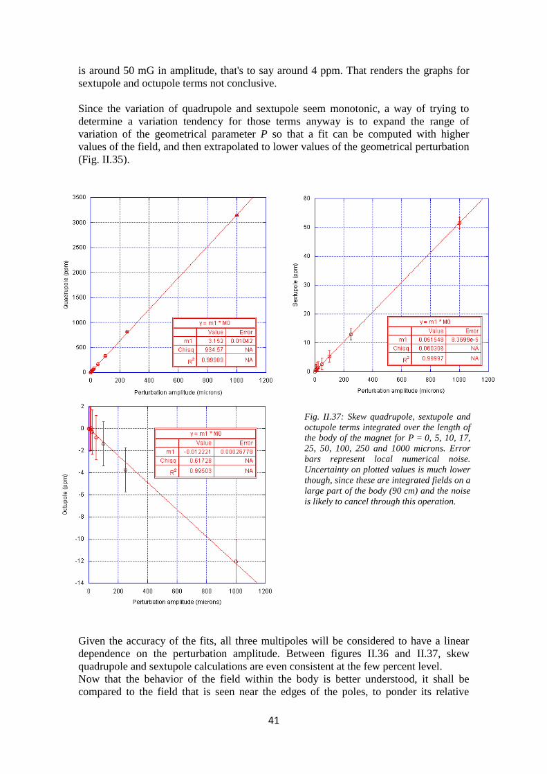
is around 50 mG in amplitude, that's to say around 4 ppm. That renders the graphs for

sextupole and octupole terms not conclusive.

Since the variation of quadrupole and sextupole seem monotonic, a way of trying to

determine a variation tendency for those terms anyway is to expand the range of

variation of the geometrical parameter P so that a fit can be computed with higher

values of the field, and then extrapolated to lower values of the geometrical perturbation

(Fig. II.35).

Given the accuracy of the fits, all three multipoles will be considered to have a linear

dependence on the perturbation amplitude. Between figures II.36 and II.37, skew

quadrupole and sextupole calculations are even consistent at the few percent level.

Now that the behavior of the field within the body is better understood, it shall be

compared to the field that is seen near the edges of the poles, to ponder its relative

Fig. II.37: Skew quadrupole, sextupole and

octupole terms integrated over the length of

the body of the magnet for P = 0, 5, 10, 17,

25, 50, 100, 250 and 1000 microns. Error

bars represent local numerical noise.

Uncertainty on plotted values is much lower

though, since these are integrated fields on a

large part of the body (90 cm) and the noise

is likely to cancel through this operation.

42

importance in the total integrated field seen by the beam as it travels through the whole

magnet.

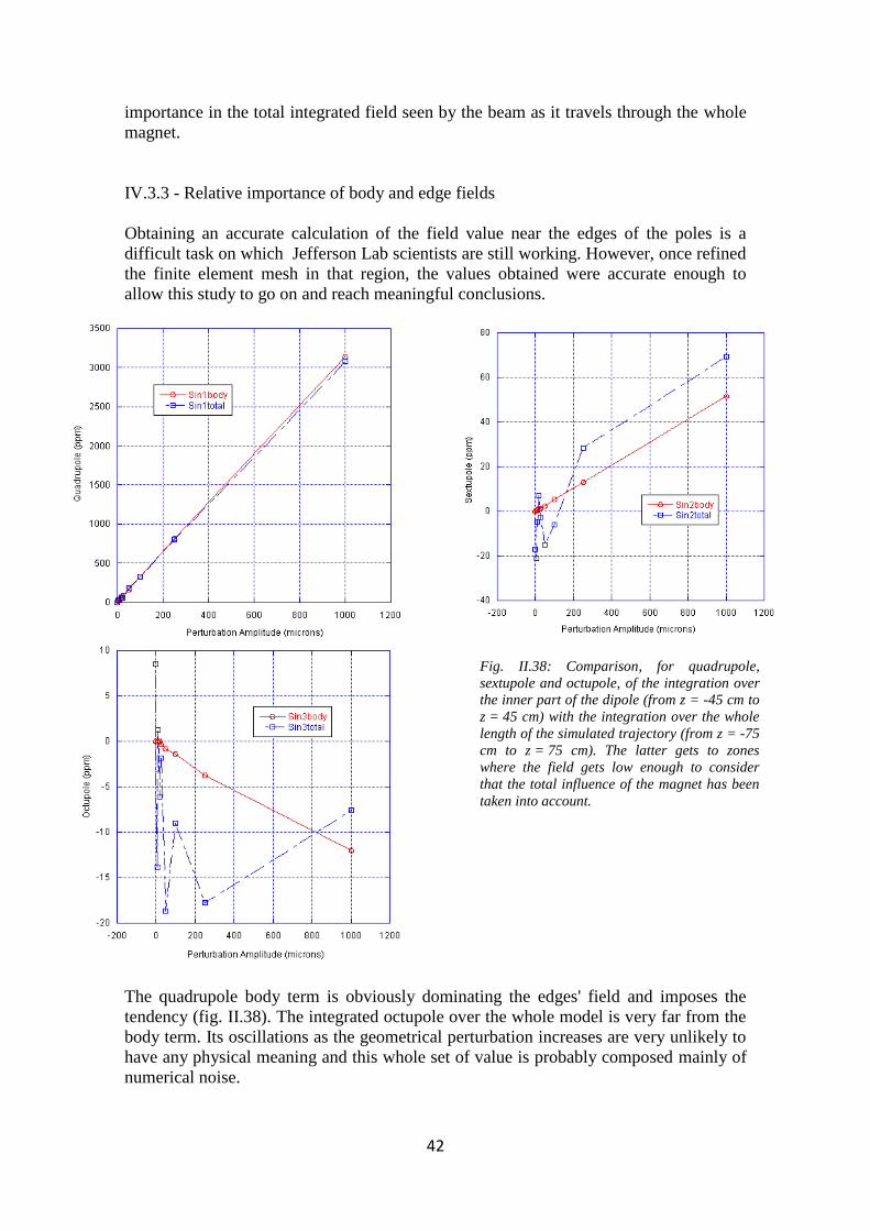
IV.3.3 - Relative importance of body and edge fields

Obtaining an accurate calculation of the field value near the edges of the poles is a

difficult task on which Jefferson Lab scientists are still working. However, once refined

the finite element mesh in that region, the values obtained were accurate enough to

allow this study to go on and reach meaningful conclusions.

The quadrupole body term is obviously dominating the edges' field and imposes the

tendency (fig. II.38). The integrated octupole over the whole model is very far from the

body term. Its oscillations as the geometrical perturbation increases are very unlikely to

have any physical meaning and this whole set of value is probably composed mainly of

numerical noise.

Fig. II.38: Comparison, for quadrupole,

sextupole and octupole, of the integration over

the inner part of the dipole (from z = -45 cm to

z = 45 cm) with the integration over the whole

length of the simulated trajectory (from z = -75

cm to z = 75 cm). The latter gets to zones

where the field gets low enough to consider

that the total influence of the magnet has been

taken into account.

43

The relation between the sextupole field integrated in the body and its integration over

the whole model seems a bit stronger for high values of the perturbation, although the

oscillation observable at low values clearly indicate that our uncertainty is too high to

establish a relation.

Conclusions

The integrated field over the body has a linear behavior with respect to the amplitude of

the geometrical perturbation of the pole tips for quadrupole, sextupole and octupole.

However, after comparison with the integrated fields over the total length of the

considered beam trajectory, it appears that a clear dominance of the body term is only

established for the quadrupole term, since the influence of numerical noise becomes too

strong when it comes to the study of higher terms, which are much lower fields.

44

VV -- GGeenneerraall ccoonncclluussiioonnss

This section presents the final conclusions that the student's work, along with his

supervisor's productive coaching led to.

1. The perturbation modeling technique is valid in the body of the magnet.

2. Skew quadrupole and sextupole calculated tendencies are consistent at the few

percent level over a variation of a factor of 20 in their evaluation domain.

3. Skew terms at the end of the steel, where perturbations terminate, are more difficult

to model. Ten variations of end mesh have been tried. One was found which did

not increase the number of elements unduly and provided more physical results than

those shown above. Unfortunately, time did not permit the work presented to be

redone with the better mesh outside the steel. The results shown here which include

the ends of the magnets are unfortunately not meaningful except to inform further

development of magnet models.

4. However, since the geometrical perturbation only affects the steel, the integrated

skew term outside of it should be close to zero, as it is in the non-perturbed models.

Use only of the terms calculated in the body of the dipole is therefore reasonable.

5. Skew terms are ~20% larger in magnets in which the steel remains in the linear

regime than in magnets approaching saturation.

6. Skew quadrupole predicted for 50 micron perturbation and 6 kG field (current

specifications for the magnets) is two orders of magnitude higher than the ~1 G per

meter of dipole seen in present CEBAF with beam. There cannot be a systematic

machining or assembly error. Errors must be random and cancel in large part OR

the vendor must have performed far better than specification, or both.

7. Skew sextupole at the level predicted would likely be seen in beam shape in the

halls and isn't. Whether it is suppressed by one or two orders of magnitude for the

same reasons as the skew quadrupole can't be determined by data available.

8. Skew terms in individual magnets immediately prior to a critical region, for instance

the Compton polarimeter chicane dipoles, should be held to tight tolerance because

there's no way to "average out" the random errors over short distances.

9. The 12 GeV project team must examine this work to determine whether they wish to

tighten the tolerance on machining of new dipoles or to gamble that the vendor

chosen will do as well as did the one who did the work in the early 1990's. Given

the large cost to tighten tolerance on the sixty or so dipoles to be purchased, perhaps

a modest incentive clause in the dipole contracts and dedicated skew correction

elements in the hall transport lines are a good strategy.

10. Extreme care must be taken in disassembly and reassembly of the existing dipoles

with H steel to ensure no systematic error is created.

11. Direct measurement of normal and skew terms through at least sextupole and

perhaps decapole is desirable so magnets can be sorted to cancel skew terms locally.

45

VVII -- RReeffeerreenncceess,, bbiibblliiooggrraapphhyy aanndd aannnneexxeess

VVII..11 -- RReeffeerreenncceess

Softwares

[1]: Opera Version 12.009 Professional Edition x64, Vector Fields Ltd, 24 Bankside,

Kidlington, Oxford, OX5 1JE, UK, support@vectorfields.co.uk,

http://www.vectorfields.com

[2]: Microsoft® Office Excel® 2007 (12.0.6214.1000) SP1 MSO (12.0.6213.1000),

Part of Microsoft Office Professional Plus 2007, © 2006 Microsoft Corporation. All

rights reserved.

[3]: Kaleidagraph Tools for discovery, Version 4.03, Copyright: 1986-2006 by Synergy

Software

[8]: Océ, Electronic Job Ticket for the Web, http://dcg4/oceweb/Oce/Main/ASP/FS_Login.asp

Books

[4]: Foster, L. W., Geo-metrics IIIm: the metric application of geometric dimensioning

and tolerancing techniques, as based upon harmonization of national and international

standard practices, ISBN 0-201-63343-4, Addison-Wesley (1994)

Publications and technical notes

[5]: J.K.Cobb, R.S.Cole, Spectroscopy of quadrupole magnets, Proc. International

Symposium on Magnet Technology (MT-1), Stanford, USA, (1965)

[6]: Y. Roblin and Arne Freyberger, Studies of Beam Halo Formation in the 12 GeV

CEBAF Design, Jlab-TN-06-048 (2006)

[7]: J. Benesh, Calculating Multipoles in Opera/TOSCA - mesh and software noise

effects, JLAB-TN-08-024 (2008)

VVII..22 -- BBiibblliiooggrraapphhyy

The following material was used in a regular basis throughout this work and would be

made reference to so often in this document that it was decided to list them as general

references in this bibliography.

Presentations

Harwood, L., A. Lung and M. Wiseman, 12 GeV ACCELERATOR OVERVIEW,

Director's Project Review, Newport News (2005)

46

Books

The American Society of Mechanical Engineers, Dimensioning and Tolerancing, ANSI

Y14.5M-1982

Wille, K., The Physics of Particle Accelerators an introduction, Oxford University

Press (2000)

American Institute of Physics, AIP CONFERENCE PROCEEDINGS 153 - PHYSICS

OF PARTICLE ACCELERATORS, SLAC Summer School 1985, Fermilab Summer

School 1984, Melvin Month & Margaret Dienes (1987)

Internet

http://www.jlab.org/

http://www.wikipedia.org/

47

VVII..33 -- LLiisstt ooff AAnnnneexxeess

[A1] : An example of a post processor output file

[A2] : The Perl script used to convert the post processor output file into a

suitable format for spreadsheet exploitation

[A3] : The script used to generate the circles along the beam path in the

post processor

[A4] : An example of a calculation report emitted by the code

48

Annex [A1]

Opera-3d Post-Processor Version 12.009 started on 25/May/2008 at 19:50:15 Copyright (c) 1984-2007, Vector Fields Limited, Oxford, UK. Node: CASNRUIZ. Processor: EM64T/x64. System: Windows XP Professional x64 Edition (Service Pack 2) Command language initialisation. Unit of Length : CM Unit of Magn Flux Den : GAUSS Unit of Magnetic Field : OERSTED Unit of Magn Scalar Pot : OCM Unit of Magn Vector Pot : GCM Unit of Conductivity : SCM Unit of Current density : ACM2 Unit of Power : WATT Unit of Force : NEWTON Unit of Energy : JOULE Unit of Electric Field : VCM Unit of Elec Flux Den : CCM2 Unit of Mass : GRAMME Information: opera.comi was not found in the local or home directory *** CONTROL COMMAND ** $COMI **** COMMAND INPUT *** **** COMMAND INPUT *** ACTIVATE FILE='C:\Documents and Settings\nruiz\My Documents\TOSCA\Spoiling\abh_jb14kG\extending models\2x100-micron_elliptic_vs_tilt\2x100-micron_elliptic_vs_tilt_extended_minus8cm.op3' Opening file for checking: C:\Documents and Settings\nruiz\My Documents\TOSCA\Spoiling\abh_jb14kG\extending models\2x100-micron_elliptic_vs_tilt\2x100-micron_elliptic_vs_tilt_extended_minus8cm.op3 **** COMMAND INPUT *** LOAD Attaching file as resident: C:\Documents and Settings\nruiz\My Documents\TOSCA\Spoiling\abh_jb14kG\extending models\2x100-micron_elliptic_vs_tilt\2x100-micron_elliptic_vs_tilt_extended_minus8cm.op3 Opening database ...liptic_vs_tilt_extended_minus8cm.op3, simulation number 1 on 25/May/2008 at 19:50:20 TITLE=z=8cm cutting plane was removed Unit of Length : CM Unit of Magn Flux Den : GAUSS Unit of Magnetic Field : OERSTED Unit of Magn Scalar Pot : OCM Unit of Magn Vector Pot : GCM Unit of Conductivity : SCM Unit of Current density : ACM2 Unit of Power : WATT Unit of Force : NEWTON Unit of Energy : JOULE Unit of Electric Field : VCM Unit of Elec Flux Den : CCM2 Unit of Mass : GRAMME **** COMMAND INPUT *** SELECT ACTION=DEFAULT **** COMMAND INPUT *** SELECT ACTION=SELECT OPTION=SURFACES **** COMMAND INPUT *** THREED OPTION=REFRESH *** CONTROL COMMAND ** $COMI 'C:\Documents and Settings\nruiz\My Documents\TOSCA\Comis\Dip_Eval_300_Nodal.comi' MODE=CONTINUOUS Opening file for input: C:\Documents and Settings\nruiz\My Documents\TOSCA\Comis\Dip_Eval_300_Nodal.comi **** FILE INPUT ****** ACTIVATE CASE=1 MODELSYMMETRY=DATABASE The resident file has been unloaded to allow the new file to be checked. Opening file for checking: C:\Documents and Settings\nruiz\My Documents\TOSCA\Spoiling\abh_jb14kG\extending models\2x100-micron_elliptic_vs_tilt\2x100-micron_elliptic_vs_tilt_extended_minus8cm.op3 **** FILE INPUT ****** LOAD Attaching file as resident: C:\Documents and Settings\nruiz\My Documents\TOSCA\Spoiling\abh_jb14kG\extending models\2x100-micron_elliptic_vs_tilt\2x100-micron_elliptic_vs_tilt_extended_minus8cm.op3 Opening database ...liptic_vs_tilt_extended_minus8cm.op3, simulation number 1 on 25/May/2008 at 19:50:53 TITLE=z=8cm cutting plane was removed Unit of Length : CM Unit of Magn Flux Den : GAUSS Unit of Magnetic Field : OERSTED Unit of Magn Scalar Pot : OCM Unit of Magn Vector Pot : GCM Unit of Conductivity : SCM Unit of Current density : ACM2 Unit of Power : WATT Unit of Force : NEWTON Unit of Energy : JOULE Unit of Electric Field : VCM Unit of Elec Flux Den : CCM2 Unit of Mass : GRAMME **** FILE INPUT ****** SELECT ACTION=DEFAULT **** FILE INPUT ****** SELECT ACTION=SELECT OPTION=SURFACES **** FILE INPUT ****** **** FILE INPUT ****** THREED OPTION=GETVIEW

49

**** FILE INPUT ****** THREED OPTION=SETVIEW ROTX=-90 ROTY=0.01 ROTZ=0.01 SIZE=100 PERSPECTIVE=NO **** FILE INPUT ****** SET FIELD=NODAL COIL=NODAL **** FILE INPUT ****** set XLOCAL=0,YLOCAL=0,ZLOCAL=0,PLOCAL=0,TLOCAL=0,SLOCAL=0 **** FILE INPUT ****** CIRCLE RADIUS=1 TH1=0 TH2=360 ZC=0 NP=60 **** FILE INPUT ****** PLOT FILE=TEMP COMPONENT=By X Y Z BY 1.0 0.0 0.0 -14163.221838764 0.99452189536827 0.10452846326765 0.0 -14162.806446465 0.97814760073381 0.20791169081776 0.0 -14162.510717193 0.95105651629515 0.30901699437495 0.0 -14162.341017265 0.9135454576426 0.4067366430758 0.0 -14162.25213583 0.86602540378444 0.5 0.0 -14162.210476839 0.80901699437495 0.58778525229247 0.0 -14162.165329251 0.74314482547739 0.66913060635886 0.0 -14162.067371641 0.66913060635886 0.74314482547739 0.0 -14161.914594433 0.58778525229247 0.80901699437495 0.0 -14161.662715689 0.5 0.86602540378444 0.0 -14161.333207984 0.4067366430758 0.9135454576426 0.0 -14160.916837241 0.30901699437495 0.95105651629515 0.0 -14160.441508285 0.20791169081776 0.97814760073381 0.0 -14159.914040818 0.10452846326765 0.99452189536827 0.0 -14159.369443517 0.0 1.0 0.0 -14158.822561159 -0.1045284632677 0.99452189536827 0.0 -14158.294760717 -0.2079116908178 0.97814760073381 0.0 -14157.783552069 -0.3090169943749 0.95105651629515 0.0 -14157.266117814 -0.4067366430758 0.9135454576426 0.0 -14156.74850479 -0.5 0.86602540378444 0.0 -14156.214193167 -0.5877852522925 0.80901699437495 0.0 -14155.658491549 -0.6691306063589 0.74314482547739 0.0 -14155.07654529 -0.7431448254774 0.66913060635886 0.0 -14154.482306533 -0.8090169943749 0.58778525229247 0.0 -14153.903318198 -0.8660254037844 0.5 0.0 -14153.369907659 -0.9135454576426 0.4067366430758 0.0 -14152.926629838 -0.9510565162952 0.30901699437495 0.0 -14152.618433451 -0.9781476007338 0.20791169081776 0.0 -14152.493506994 -0.9945218953683 0.10452846326765 0.0 -14152.589940569 -1.0 0.0 0.0 -14152.932915504 -0.9945218953683 -0.1045284632677 0.0 -14153.51801096 -0.9781476007338 -0.2079116908178 0.0 -14154.343419998 -0.9510565162952 -0.3090169943749 0.0 -14155.378395705 -0.9135454576426 -0.4067366430758 0.0 -14156.582637608 -0.8660254037844 -0.5 0.0 -14157.865888133 -0.8090169943749 -0.5877852522925 0.0 -14159.213505653 -0.7431448254774 -0.6691306063589 0.0 -14160.557094496 -0.6691306063589 -0.7431448254774 0.0 -14161.848552429 -0.5877852522925 -0.8090169943749 0.0 -14163.059517056 -0.5 -0.8660254037844 0.0 -14164.168265547 -0.4067366430758 -0.9135454576426 0.0 -14165.170902605 -0.3090169943749 -0.9510565162952 0.0 -14166.062913137 -0.2079116908178 -0.9781476007338 0.0 -14166.853519502 -0.1045284632677 -0.9945218953683 0.0 -14167.551863513 0.0 -1.0 0.0 -14168.162896764 0.10452846326765 -0.9945218953683 0.0 -14168.683218789 0.20791169081776 -0.9781476007338 0.0 -14169.099039803 0.30901699437495 -0.9510565162952 0.0 -14169.392133901 0.4067366430758 -0.9135454576426 0.0 -14169.536789695 0.5 -0.8660254037844 0.0 -14169.512690175 0.58778525229247 -0.8090169943749 0.0 -14169.312312022 0.66913060635886 -0.7431448254774 0.0 -14168.937056385 0.74314482547739 -0.6691306063589 0.0 -14168.400606992 0.80901699437495 -0.5877852522925 0.0 -14167.720236367 0.86602540378444 -0.5 0.0 -14166.925138756 0.9135454576426 -0.4067366430758 0.0 -14166.098348065 0.95105651629515 -0.3090169943749 0.0 -14165.265408849 0.97814760073381 -0.2079116908178 0.0 -14164.482016017 0.99452189536827 -0.1045284632677 0.0 -14163.783981529 1.0 0.0 0.0 -14163.221838764 Component: BY, from buffer: Circle Minimum: -14169.5367896953, Maximum: -14152.4935069936 Integral = -88936.9800883494 **** FILE INPUT ****** FIT TYPE=FOURIER FILE=TEMP COMP=By ORDER=10 PRINT=YES Polynomial fitting to tabulated values on a line Component: BY Fourier coefficients Order Sine term Cosine term Amplitude Phase n A_n B_n 0 0.0 -14161.229928783 14161.2299287827 179.999994991044 1 4.65362551353294 -5.1715594743102 6.95710125099044 -138.01754624113 2 0.06511040232441 2.71085332286577 2.7116351344868 -1.3758892829255 3 -0.018629312841 0.02822737628213 0.03382064559852 33.4237420306027 4 -6.226690931E-05 0.44176275077825 0.44176275516654 8.0758981544E-03 5 -3.156967654E-03 -3.641395952E-03 4.8193577627E-03 139.075809756733 6 1.463015892E-03 -1.04168556E-03 1.7959744724E-03 -125.45133672036 7 8.1625057096E-04 4.8987181458E-06 8.1626527062E-04 -89.656141690398 8 4.9866337026E-04 2.3009152433E-03 2.3543313517E-03 -12.228255562204

50

9 1.3782763069E-04 -7.529855982E-04 7.654957654E-04 -169.62731411444 **** FILE INPUT ****** set xloc=1.374,0.000,74.981,2.699,0.000,0.000 **** FILE INPUT ****** circ **** FILE INPUT ****** fit Polynomial fitting to tabulated values on a line Component: BY Fourier coefficients Order Sine term Cosine term Amplitude Phase n A_n B_n 0 0.0 -5.4555288062005 5.45552880620054 179.999994991044 1 -0.0168299773886 -0.1707010108206 0.17152866592515 174.369212576266 2 5.0776727173E-03 0.03383178578031 0.03421070723193 -8.5355765642261 3 0.01432123088062 -1.856113384E-03 0.01444101141992 -97.38469293707 4 -6.691231953E-03 1.3234512454E-03 6.8208583218E-03 78.8119324375829 5 -2.823309362E-03 -4.974628375E-03 5.719965316E-03 150.423275375887 6 8.1448365678E-03 0.01101269519737 0.01369736537539 -36.486114453426 7 6.191892909E-03 9.2542828953E-03 0.01113468857686 -33.785847576462 8 -1.445175793E-03 9.037727344E-03 9.1525432868E-03 9.08495700215354 9 -5.90514075E-03 1.6497468997E-03 6.1312602381E-03 74.3909795088685 **** FILE INPUT ****** set xloc=1.362,0.000,74.731,2.690,0.000,0.000 **** FILE INPUT ****** circ **** FILE INPUT ****** fit Polynomial fitting to tabulated values on a line Component: BY Fourier coefficients Order Sine term Cosine term Amplitude Phase n A_n B_n 0 0.0 -5.3960906761972 5.39609067619721 179.999994991044 1 -6.303748054E-03 -0.1757395096984 0.17585253057193 177.945685371731 2 -1.724816197E-03 0.04217618394546 0.04221143782336 2.34183463045649 3 0.01593779981791 -6.554857298E-03 0.01723309656526 -112.35625622872 4 2.8109563302E-03 7.1221023268E-03 7.6567497702E-03 -21.538192197483 5 3.0424887929E-03 -2.715035426E-03 4.0777635316E-03 -131.74486353951 6 -4.610919032E-03 6.9654883587E-03 8.3533587491E-03 33.5032184210446 7 1.6607229841E-03 0.01022753106116 0.0103614860149 -9.2230589314923 8 5.1316060632E-03 4.0134610763E-03 6.5146949736E-03 -51.970814350807 9 5.1507520595E-03 -2.623088254E-03 5.7802109622E-03 -116.98806465358 **** FILE INPUT ****** set xloc=1.350,0.000,74.481,2.681,0.000,0.000 **** FILE INPUT ****** circ **** FILE INPUT ****** fit Polynomial fitting to tabulated values on a line Component: BY Fourier coefficients Order Sine term Cosine term Amplitude Phase n A_n B_n 0 0.0 -5.3226354037128 5.32263540371283 179.999994991044 1 3.5975865751E-03 -0.1793324295713 0.1793685115206 -178.85073895747 2 -3.540815259E-03 0.03329422539948 0.03348197750509 6.07054425273992 3 8.0464508355E-03 6.8704450932E-03 0.01058056647002 -49.507711780297 4 -0.0181358052348 -6.80834172E-03 0.01937165322033 110.576576514822 5 -4.799463861E-03 -1.001028752E-03 4.9027453449E-03 101.781333762995 6 -1.581774896E-03 -5.037607792E-03 5.2801045529E-03 162.56805835838 7 -6.340173195E-04 0.01622444987614 0.01623683318092 2.23785962239485 8 -2.00519836E-03 5.8541896055E-03 6.1880818029E-03 18.907544000601 9 3.3446749663E-03 -7.721660831E-04 3.4326507382E-03 -102.99978609285 **** FILE INPUT ****** set xloc=1.338,0.000,74.232,2.672,0.000,0.000 **** FILE INPUT ****** circ **** FILE INPUT ****** fit Polynomial fitting to tabulated values on a line Component: BY Fourier coefficients Order Sine term Cosine term Amplitude Phase n A_n B_n 0 0.0 -5.2365498124121 5.2365498124121 179.999994991044 1 9.6710022669E-03 -0.1630760471865 0.16336255828933 -176.60612206643 2 0.01765975976018 0.01972255920183 0.02647350479738 -41.841554870655 3 -9.447436244E-03 6.0596624357E-03 0.01122379438613 57.3235558030462 4 -5.783492371E-03 -0.0179566940429 0.01886509064256 162.147282956251 5 -6.828364476E-03 3.3041885457E-03 7.585790886E-03 64.1780461042141 6 8.9752446137E-03 -2.053754204E-03 9.207221199E-03 -102.88876787707 7 -3.182523228E-03 0.01109710489124 0.01154444416432 16.0022876545783 8 -8.947663227E-03 3.0604180317E-04 8.9528955543E-03 88.041042446106 9 2.9118555872E-03 0.01248614979323 0.0128211871377 -13.127148647153 **** FILE INPUT ****** set xloc=1.327,0.000,73.982,2.663,0.000,0.000 **** FILE INPUT ****** circ **** FILE INPUT ****** fit Polynomial fitting to tabulated values on a line Component: BY Fourier coefficients Order Sine term Cosine term Amplitude Phase n A_n B_n 0 0.0 -5.1399744669276 5.13997446692761 179.999994991044 1 0.01784765672023 -0.1611717519349 0.16215693778607 -173.68098474899 2 0.01308234533318 0.0217545679869 0.02538521198874 -31.021052524404 3 -1.263289006E-03 5.9076636117E-03 6.0412240864E-03 12.0702845141411 4 4.8439101676E-03 -6.797978796E-03 8.3472139919E-03 -144.5281656903

51

5 7.6228602747E-04 -4.313425215E-03 4.3802644979E-03 -169.97793168579 6 7.0224167183E-03 5.7685872572E-03 9.0879555187E-03 -50.598492566929 7 -4.831385993E-04 0.01411432841265 0.0141225949969 1.9604898598809 8 -6.320537285E-04 6.1656790677E-03 6.1979908262E-03 5.85303748566267 9 -3.348580958E-03 8.9390734754E-03 9.5456811717E-03 20.5359719157808 **** FILE INPUT ****** set xloc=1.315,0.000,73.732,2.654,0.000,0.000 **** FILE INPUT ****** circ **** FILE INPUT ****** fit Polynomial fitting to tabulated values on a line Component: BY Fourier coefficients Order Sine term Cosine term Amplitude Phase n A_n B_n 0 0.0 -5.0447333605769 5.04473336057689 179.999994991044 1 0.02123581632123 -0.1526867354578 0.15415641108815 -172.08203671952 2 4.1953513972E-03 1.8289375564E-04 4.1993360752E-03 -87.503803921773 3 -0.0160653871389 -0.0130001118032 0.02066638746413 128.979781825153 4 3.422772327E-03 6.7299790728E-03 7.5503634828E-03 -26.957245081729 5 6.0712280479E-03 -2.878639534E-03 6.7191052661E-03 -115.36770967612 6 9.887445942E-03 -3.192005559E-03 0.0103899223647 -107.89185025874 7 -3.013360418E-03 0.01294211458046 0.01328829074108 13.1068701351751 8 9.0359476595E-03 2.4155459052E-03 9.3532460742E-03 -75.033304737512 9 -5.831596302E-03 9.9000123276E-03 0.0114898981509 30.5001855306647 **** FILE INPUT ****** set xloc=1.304,0.000,73.482,2.645,0.000,0.000 **** FILE INPUT ****** circ **** FILE INPUT ****** fit Polynomial fitting to tabulated values on a line Component: BY Fourier coefficients Order Sine term Cosine term Amplitude Phase n A_n B_n 0 0.0 -4.9478856805132 4.94788568051322 179.999994991044 1 0.01050345038872 -0.1604141346341 0.16075763453248 -176.25378184841 2 -0.0140916820987 0.01032898438486 0.01747178934151 53.7591605019161 3 -3.685393007E-03 -8.486052151E-03 9.2517675457E-03 156.525254286864 4 6.4949583244E-04 9.1377633271E-03 9.1608167462E-03 -4.0656436625791 5 3.9731102382E-03 -0.0125276007275 0.01314254103862 -162.40364732435 6 2.775600168E-04 4.5848136044E-03 4.593207523E-03 -3.4644007444617 7 -9.681876291E-03 -2.748728041E-03 0.01006450368206 105.849478872961 8 3.78303312E-03 0.01401998437927 0.01452140838838 -15.100574838281 9 -1.42780682E-03 0.01130736659921 0.01139715629987 7.19677896128044 **** FILE INPUT ****** set xloc=1.292,0.000,73.232,2.636,0.000,0.000 **** FILE INPUT ****** circ **** FILE INPUT ****** fit Polynomial fitting to tabulated values on a line Component: BY Fourier coefficients Order Sine term Cosine term Amplitude Phase n A_n B_n 0 0.0 -4.8401295503025 4.84012955030248 179.999994991044 1 8.9290400378E-03 -0.164845536941 0.16508718546682 -176.89953593107 2 -0.0150331387836 -7.39200321E-04 0.01505130156502 92.8150432003212 3 -9.466765608E-03 -0.0126126271511 0.01577016216573 143.108894442669 4 -4.12096114E-03 6.2448534677E-03 7.482012801E-03 33.4207061061371 5 -0.0126769018456 -0.0290687968947 0.03171275442634 156.437980548225 6 7.9278630479E-03 8.1819275815E-03 0.0113927587289 -44.096472516201 7 -8.062370716E-03 -6.563520868E-03 0.01039623142075 129.148796086931 8 0.01070028932416 0.01043341965579 0.01494498033905 -45.72347291939 9 -6.382300157E-03 5.6676717275E-05 6.3825518048E-03 89.4912073776728 **** FILE INPUT ****** set xloc=1.281,0.000,72.983,2.627,0.000,0.000 **** FILE INPUT ****** circ **** FILE INPUT ****** fit Polynomial fitting to tabulated values on a line Component: BY Fourier coefficients Order Sine term Cosine term Amplitude Phase n A_n B_n 0 0.0 -4.7256698636916 4.72566986369159 179.999994991044 1 0.0103644251464 -0.1719950980788 0.1723070952449 -176.55152131145 2 -6.198996998E-03 -4.612937322E-03 7.7270145928E-03 126.654500287176 3 -0.0200267375188 5.1584525719E-03 0.0206804218667 75.5558267270421 4 -4.546729998E-03 -2.961238211E-03 5.4260192971E-03 123.075778533519 5 7.3149632177E-04 -0.0224369588587 0.02244887992071 -178.13268262058 6 -0.0104595995942 1.4424625171E-03 0.01055859468798 82.1479792522418 7 -8.089557457E-03 3.1051841128E-03 8.6650509646E-03 69.0006527627503 8 8.1664482581E-03 -1.804387129E-03 8.3634137805E-03 -102.45939294564 9 -5.518281661E-04 -4.189042044E-03 4.2252322506E-03 172.495554273329 **** FILE INPUT ****** set xloc=1.269,0.000,72.733,2.618,0.000,0.000 **** FILE INPUT ****** circ **** FILE INPUT ****** fit Polynomial fitting to tabulated values on a line Component: BY Fourier coefficients Order Sine term Cosine term Amplitude Phase n A_n B_n 0 0.0 -4.6233375157648 4.62333751576476 179.999994991044

52

1 0.0219927667348 -0.1837783390834 0.18508959912679 -173.17585773406 2 -2.581049507E-03 -0.0147597499746 0.0149837257005 170.080931732679 3 -0.0178124855031 9.8648630972E-03 0.0203617328271 61.0215545940324 4 -0.0213738261309 -9.758817403E-03 0.02349627546201 114.540389721903 5 0.01377321290566 -1.247675632E-03 0.01382960911331 -95.176129122927 6 -1.459649679E-03 -0.012983218081 0.01306501163123 173.585402329276 7 -7.281407948E-03 -3.991718258E-03 8.3037772346E-03 118.731854980857 8 1.6930444232E-03 -3.298373776E-03 3.7075152035E-03 -152.82871514724 9 0.01945241172045 -5.741288033E-03 0.02028197993353 -106.44371492917 **** FILE INPUT ****** set xloc=1.258,0.000,72.483,2.609,0.000,0.000 **** FILE INPUT ****** circ **** FILE INPUT ****** fit Polynomial fitting to tabulated values on a line Component: BY Fourier coefficients Order Sine term Cosine term Amplitude Phase n A_n B_n 0 0.0 -4.5005921992228 4.50059219922278 179.999994991044 1 0.02243467518584 -0.180034604897 0.18142704762828 -172.89680501802 2 5.2984666972E-03 -0.0147610095509 0.01568314867314 -160.25438731864 3 -0.0183075303818 -3.298442573E-03 0.01860229534456 100.213328939248 4 -0.0199270464637 -0.0277422731559 0.03415729644783 144.31061987589 5 0.01173882328007 3.6262131214E-04 0.01174442277069 -88.230649340856 6 1.285607817E-03 -0.0226197465026 0.02265625121906 -176.74705229987 7 -6.213143399E-03 -2.855661608E-03 6.837978803E-03 114.68427663074 8 -3.976529788E-03 -0.0131604385863 0.01374808833749 163.187391614213 9 1.9868299109E-03 1.7160682256E-03 2.6253348834E-03 -49.182112372073 **** FILE INPUT ****** set xloc=1.246,0.000,72.233,2.600,0.000,0.000 **** FILE INPUT ****** circ **** FILE INPUT ****** fit Polynomial fitting to tabulated values on a line Component: BY Fourier coefficients Order Sine term Cosine term Amplitude Phase n A_n B_n 0 0.0 -4.3644466324416 4.36444663244158 179.999994991044 1 0.02332330005347 -0.1729240278609 0.17448981556816 -172.31852542825 2 9.2438590244E-03 -0.0126348791979 0.01565532184305 -143.81025778957 3 -1.873216912E-03 -1.866459026E-03 2.6443545329E-03 134.896458416811 4 -0.0192091270998 -0.0382454949587 0.04279846315665 153.331513495255 5 0.01498818203654 1.0703062619E-03 0.0150263487333 -85.915438799075 6 -0.0127514724869 -0.0419697613491 0.04386411880207 163.099890437751 7 0.01162286111938 -0.0113507226872 0.01624591659843 -134.32131876523 8 -9.478348447E-03 5.759649181E-04 9.4958319736E-03 86.5226164461483 9 -6.84564669E-03 1.9479293266E-03 7.1173946964E-03 74.1162906848878 **** FILE INPUT ****** set xloc=1.235,0.000,71.984,2.591,0.000,0.000 **** FILE INPUT ****** circ **** FILE INPUT ****** fit Polynomial fitting to tabulated values on a line Component: BY Fourier coefficients Order Sine term Cosine term Amplitude Phase n A_n B_n 0 0.0 -4.2497924492698 4.2497924492698 179.999994991044 1 0.01278048625356 -0.1864177300278 0.18685532076336 -176.07802980255 2 -0.024654278111 0.02814582883659 0.0374168559619 41.2166678101678 3 0.01341738686851 2.7828163464E-03 0.0137029317008 -78.282764051757 4 -0.0181170493595 -0.0100635464954 0.020724440778 119.051021776109 5 7.8901662887E-03 4.3430835541E-03 9.0065031406E-03 -61.169739139982 6 -0.0269781552644 -4.119739513E-03 0.02729089802712 98.6823607061154 7 9.3766193909E-03 -0.0153852218786 0.01801738170364 -148.63951671479 8 0.01264267600445 -6.945726336E-03 0.01442499119205 -118.78383379546 9 6.5057957104E-03 1.9653220975E-04 6.5087635335E-03 -88.269687646523 **** FILE INPUT ****** set xloc=1.224,0.000,71.734,2.582,0.000,0.000 **** FILE INPUT ****** circ **** FILE INPUT ****** fit Polynomial fitting to tabulated values on a line Component: BY Fourier coefficients Order Sine term Cosine term Amplitude Phase n A_n B_n 0 0.0 -4.1051794781058 4.10517947810584 179.999994991044 1 -6.115662756E-03 -0.1801752178958 0.18027897956985 178.055958601917 2 -0.0389153307612 9.720159284E-03 0.04011090206868 75.975773890947 3 1.4082093542E-03 0.02232540957081 0.02236977796245 -3.6092372620495 4 -0.0179579684649 0.01096367091403 0.02104021652215 58.5951633764696 5 -1.366461955E-03 0.02355019550527 0.02358980556536 3.32077137014595 6 4.0295633064E-03 0.019958819678 0.02036152900397 -11.414231214432 7 2.3216657447E-03 -1.02433911E-03 2.5375977698E-03 -113.80748576549 8 4.4739221979E-04 3.8685756914E-03 3.8943597263E-03 -6.5968245676143 9 8.6234316793E-03 4.3274088292E-04 8.6342827495E-03 -87.12719171419 **** FILE INPUT ****** set xloc=1.213,0.000,71.484,2.573,0.000,0.000 **** FILE INPUT ****** circ **** FILE INPUT ****** fit Polynomial fitting to tabulated values on a line Component: BY

53

Fourier coefficients Order Sine term Cosine term Amplitude Phase n A_n B_n 0 0.0 -3.9423143112273 3.94231431122734 179.999994991044 1 1.1001155694E-03 -0.1737131538566 0.17371663730653 -179.63714892377 2 -0.0175869721928 7.969056105E-04 0.01760501773531 87.4055704644047 3 -0.0126037664606 9.781224356E-03 0.01595391108457 52.1865451127314 4 -3.151805431E-03 0.01115816064694 0.01159475857857 15.7732024650905 5 -2.22073355E-03 8.0672348484E-03 8.3673135233E-03 15.3910665307226 6 0.0142643794998 -1.193819784E-03 0.01431424913126 -94.784068089167 7 -8.805528549E-03 -8.040709259E-04 8.8421639361E-03 95.2174535005397 8 -0.0133916704794 -3.872211833E-03 0.01394026049633 106.127263218246 9 -2.433923257E-03 -7.020755753E-03 7.4306792259E-03 160.879822875449 **** FILE INPUT ****** set xloc=1.201,0.000,71.234,2.564,0.000,0.000 **** FILE INPUT ****** circ **** FILE INPUT ****** fit Polynomial fitting to tabulated values on a line Component: BY Fourier coefficients Order Sine term Cosine term Amplitude Phase n A_n B_n 0 0.0 -3.7814111632706 3.78141116327056 179.999994991044 1 8.1509087264E-03 -0.1900788496673 0.19025353190917 -177.54455758571 2 0.01695483801069 -0.0100733520207 0.01972153525722 -120.71574927529 3 -0.0262924768067 2.7118900243E-03 0.02643196330461 84.1111519321674 4 0.01072770693989 1.2448113038E-03 0.01079968755891 -83.381166025254 5 1.7758531526E-03 -4.275854915E-03 4.6299664873E-03 -157.44584829101 6 0.01455836544061 -0.0169165809629 0.02231852853072 -139.28479511806 7 -1.474641101E-03 -0.0122102870099 0.0122990111489 173.113712348495 8 4.3157423451E-03 5.8183169669E-03 7.2442007369E-03 -36.566211439185 9 -2.806533209E-03 -0.0164959014511 0.01673294335556 170.344422261072 **** FILE INPUT ****** set xloc=1.190,0.000,70.985,2.555,0.000,0.000 **** FILE INPUT ****** circ **** FILE INPUT ****** fit Polynomial fitting to tabulated values on a line Component: BY Fourier coefficients Order Sine term Cosine term Amplitude Phase n A_n B_n 0 0.0 -3.6557890419703 3.65578904197028 179.999994991044 1 9.4086848809E-03 -0.189368306612 0.18960189582459 -177.15561726328 2 0.01573703177383 -0.0125652628203 0.02013802370626 -128.60567847531 3 -0.0104008589286 -0.0145011131213 0.01784545175139 144.350181633111 4 5.0414200392E-03 3.9538449793E-03 6.4069342226E-03 -51.893899047621 5 0.01347977084369 -5.936967453E-03 0.01472928391123 -113.77038537408 6 -0.0130196940196 -0.0137663111658 0.0189479221942 136.596611214775 7 -8.534104531E-03 -9.51401277E-03 0.01278074251079 138.107773770795 8 2.2154564125E-03 -0.0101159624378 0.01035572031096 -167.64691121537 9 5.8455455992E-03 -9.123273069E-04 5.9163117284E-03 -98.870713111373 **** FILE INPUT ****** set xloc=1.179,0.000,70.735,2.546,0.000,0.000 **** FILE INPUT ****** circ **** FILE INPUT ****** fit Polynomial fitting to tabulated values on a line Component: BY Fourier coefficients Order Sine term Cosine term Amplitude Phase n A_n B_n 0 0.0 -3.4951991519081 3.49519915190815 179.999994991044 1 -0.0164025012607 -0.1779722672294 0.17872652279498 174.734305716263 2 3.8519185985E-03 9.6521322079E-03 0.01039234973661 -21.75567482537 3 -3.37024042E-03 0.0105843241364 0.01110794481061 17.662416454959 4 3.7299243687E-03 5.1973648317E-03 6.3972601158E-03 -35.665370069252 5 0.01105203040909 3.5256122496E-03 0.01160074643708 -72.307246656238 6 -0.0225954090602 7.4623691127E-03 0.02379578667265 71.7236538546793 7 -2.350890087E-03 -0.0126258814136 0.01284287996011 169.452526820164 8 -0.010813291612 -6.64160277E-03 0.01269008127776 121.558546895691 9 5.9394803992E-03 2.1628634465E-03 6.3210288483E-03 -69.99088947862 **** FILE INPUT ****** set xloc=1.168,0.000,70.485,2.537,0.000,0.000 **** FILE INPUT ****** circ **** FILE INPUT ****** fit Polynomial fitting to tabulated values on a line Component: BY Fourier coefficients Order Sine term Cosine term Amplitude Phase n A_n B_n 0 0.0 -3.3383440052784 3.33834400527838 179.999994991044 1 -0.016652837716 -0.1693721247774 0.17018881765737 174.384664553673 2 -0.0135099630128 0.01068602641471 0.01722527971163 51.6569260388887 3 3.7455166458E-03 -3.413603167E-03 5.0676998261E-03 -132.34553125859 4 5.4674784524E-03 0.0203582419118 0.02107964265274 -15.03282809465 5 4.4634628352E-03 5.8157895471E-03 7.3311601086E-03 -37.505272725832 6 -0.0190774103469 0.0114991173963 0.02227503729372 58.9200680400118 7 -3.551419199E-03 -5.203454444E-03 6.2998822588E-03 145.685997149324 8 -5.45530537E-03 -3.649007139E-04 5.4674956986E-03 93.8267627231636 9 1.7540300152E-03 -1.676077308E-03 2.4260784067E-03 -133.69811501093 **** FILE INPUT ****** set xloc=1.157,0.000,70.235,2.528,0.000,0.000

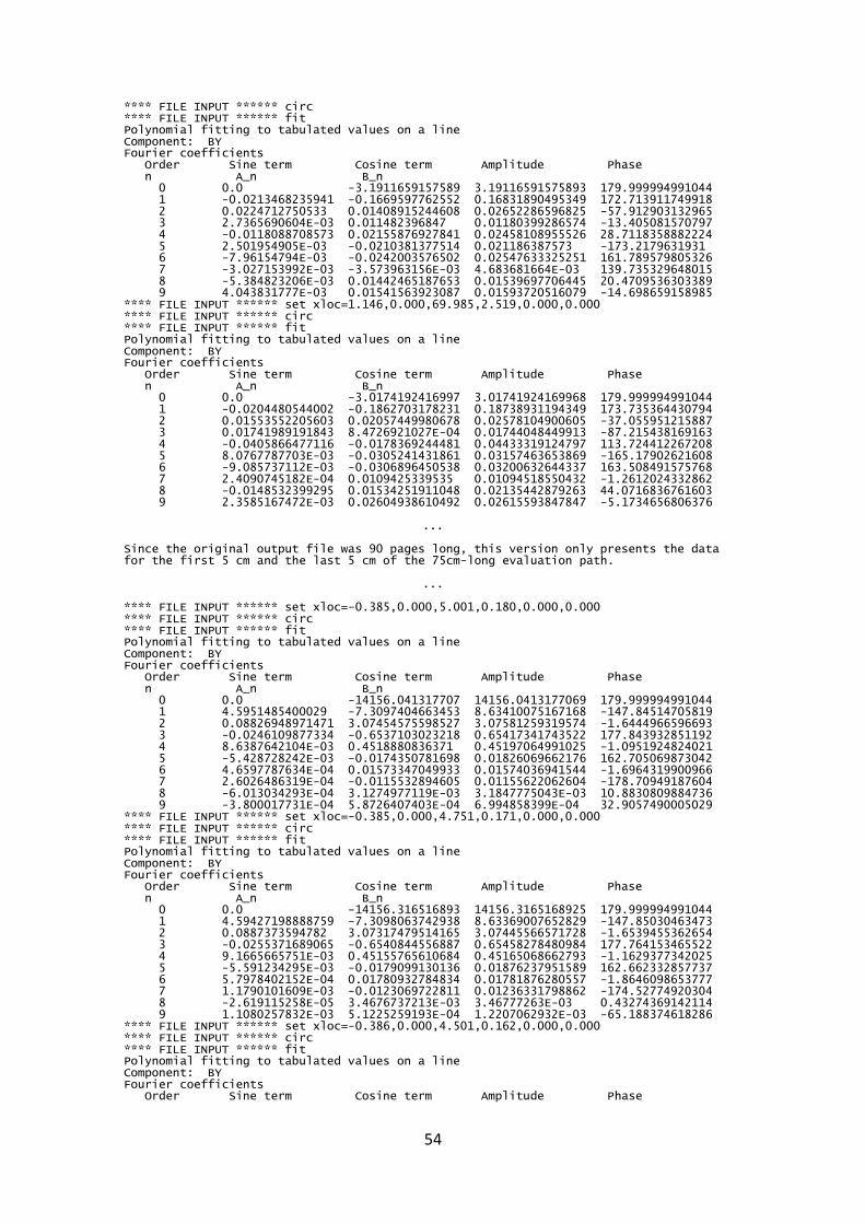
54

**** FILE INPUT ****** circ **** FILE INPUT ****** fit Polynomial fitting to tabulated values on a line Component: BY Fourier coefficients Order Sine term Cosine term Amplitude Phase n A_n B_n 0 0.0 -3.1911659157589 3.19116591575893 179.999994991044 1 -0.0213468235941 -0.1669597762552 0.16831890495349 172.713911749918 2 0.0224712750533 0.01408915244608 0.02652286596825 -57.912903132965 3 2.7365690604E-03 0.011482396847 0.01180399286574 -13.405081570797 4 -0.0118088708573 0.02155876927841 0.02458108955526 28.7118358882224 5 2.501954905E-03 -0.0210381377514 0.021186387573 -173.2179631931 6 -7.96154794E-03 -0.0242003576502 0.02547633325251 161.789579805326 7 -3.027153992E-03 -3.573963156E-03 4.683681664E-03 139.735329648015 8 -5.384823206E-03 0.01442465187653 0.01539697706445 20.4709536303389 9 4.043831777E-03 0.01541563923087 0.01593720516079 -14.698659158985 **** FILE INPUT ****** set xloc=1.146,0.000,69.985,2.519,0.000,0.000 **** FILE INPUT ****** circ **** FILE INPUT ****** fit Polynomial fitting to tabulated values on a line Component: BY Fourier coefficients Order Sine term Cosine term Amplitude Phase n A_n B_n 0 0.0 -3.0174192416997 3.01741924169968 179.999994991044 1 -0.0204480544002 -0.1862703178231 0.18738931194349 173.735364430794 2 0.01553552205603 0.02057449980678 0.02578104900605 -37.055951215887 3 0.01741989191843 8.4726921027E-04 0.01744048449913 -87.215438169163 4 -0.0405866477116 -0.0178369244481 0.04433319124797 113.724412267208 5 8.0767787703E-03 -0.0305241431861 0.03157463653869 -165.17902621608 6 -9.085737112E-03 -0.0306896450538 0.03200632644337 163.508491575768 7 2.4090745182E-04 0.0109425339535 0.01094518550432 -1.2612024332862 8 -0.0148532399295 0.01534251911048 0.02135442879263 44.0716836761603 9 2.3585167472E-03 0.02604938610492 0.02615593847847 -5.1734656806376

... Since the original output file was 90 pages long, this version only presents the data for the first 5 cm and the last 5 cm of the 75cm-long evaluation path.

... **** FILE INPUT ****** set xloc=-0.385,0.000,5.001,0.180,0.000,0.000 **** FILE INPUT ****** circ **** FILE INPUT ****** fit Polynomial fitting to tabulated values on a line Component: BY Fourier coefficients Order Sine term Cosine term Amplitude Phase n A_n B_n 0 0.0 -14156.041317707 14156.0413177069 179.999994991044 1 4.5951485400029 -7.3097404663453 8.63410075167168 -147.84514705819 2 0.08826948971471 3.07454575598527 3.07581259319574 -1.6444966596693 3 -0.0246109877334 -0.6537103023218 0.65417341743522 177.843932851192 4 8.6387642104E-03 0.4518880836371 0.45197064991025 -1.0951924824021 5 -5.428728242E-03 -0.0174350781698 0.01826069662176 162.705069873042 6 4.6597787634E-04 0.01573347049933 0.01574036941544 -1.6964319900966 7 2.6026486319E-04 -0.0115532894605 0.01155622062604 -178.70949187604 8 -6.013034293E-04 3.1274977119E-03 3.1847775043E-03 10.8830809884736 9 -3.800017731E-04 5.8726407403E-04 6.994858399E-04 32.9057490005029 **** FILE INPUT ****** set xloc=-0.385,0.000,4.751,0.171,0.000,0.000 **** FILE INPUT ****** circ **** FILE INPUT ****** fit Polynomial fitting to tabulated values on a line Component: BY Fourier coefficients Order Sine term Cosine term Amplitude Phase n A_n B_n 0 0.0 -14156.316516893 14156.3165168925 179.999994991044 1 4.59427198888759 -7.3098063742938 8.63369007652829 -147.85030463473 2 0.0887373594782 3.07317479514165 3.07445566571728 -1.6539455362654 3 -0.0255371689065 -0.6540844556887 0.65458278480984 177.764153465522 4 9.1665665751E-03 0.45155765610684 0.45165068662793 -1.1629377342025 5 -5.591234295E-03 -0.0179099130136 0.01876237951589 162.662332857737 6 5.7978402152E-04 0.01780932784834 0.01781876280557 -1.8646098653777 7 1.1790101609E-03 -0.0123069722811 0.01236331798862 -174.52774920304 8 -2.619115258E-05 3.4676737213E-03 3.46777263E-03 0.43274369142114 9 1.1080257832E-03 5.1225259193E-04 1.2207062932E-03 -65.188374618286 **** FILE INPUT ****** set xloc=-0.386,0.000,4.501,0.162,0.000,0.000 **** FILE INPUT ****** circ **** FILE INPUT ****** fit Polynomial fitting to tabulated values on a line Component: BY Fourier coefficients Order Sine term Cosine term Amplitude Phase

55

n A_n B_n 0 0.0 -14156.568206666 14156.5682066664 179.999994991044 1 4.59524879477979 -7.3167174291913 8.64006165629374 -147.86920797982 2 0.08861482685431 3.07865282837395 3.07992789285615 -1.6487256778701 3 -0.0252585491024 -0.6573739831733 0.65785906397642 177.799578351724 4 9.2669440085E-03 0.45250199889881 0.45259687941774 -1.1732159360174 5 -6.66074035E-03 -0.0167486082263 0.01802446502735 158.312814880565 6 3.7866494438E-04 0.0156231907003 0.01562777894641 -1.3884267339699 7 3.6361800472E-04 -0.0112738241858 0.01127968660142 -178.15265762608 8 -5.938749438E-05 2.167359264E-03 2.1681727454E-03 1.56956050195495 9 8.9195422295E-04 -5.385171848E-04 1.0419131894E-03 -121.12146816221 **** FILE INPUT ****** set xloc=-0.387,0.000,4.250,0.153,0.000,0.000 **** FILE INPUT ****** circ **** FILE INPUT ****** fit Polynomial fitting to tabulated values on a line Component: BY Fourier coefficients Order Sine term Cosine term Amplitude Phase n A_n B_n 0 0.0 -14156.809536304 14156.8095363039 179.999994991044 1 4.59580924557914 -7.3198122079814 8.64298058437387 -147.87697311984 2 0.09062567627986 3.07882876040227 3.08016226018718 -1.6860209433793 3 -0.0250227112021 -0.659663417032 0.66013783397581 177.827661915806 4 0.01036629086909 0.45391340593383 0.45403176108378 -1.308270400441 5 -3.756424636E-03 -0.0190566095737 0.01942331316973 168.848856803027 6 9.7488853613E-04 0.01850433953311 0.0185300024073 -3.015800875532 7 6.4872970064E-04 -0.0138413415329 0.01385653584615 -177.31656348769 8 3.5853526084E-04 4.9311533615E-03 4.9441704065E-03 -4.1585548619044 9 9.5133143078E-04 -8.613100132E-04 1.2833107301E-03 -132.15684546337 **** FILE INPUT ****** set xloc=-0.388,0.000,4.000,0.144,0.000,0.000 **** FILE INPUT ****** circ **** FILE INPUT ****** fit Polynomial fitting to tabulated values on a line Component: BY Fourier coefficients Order Sine term Cosine term Amplitude Phase n A_n B_n 0 0.0 -14157.0334308 14157.0334308004 179.999994991044 1 4.59242866874457 -7.3260645746097 8.64648039544755 -147.9179755991 2 0.09104169946606 3.08130036699055 3.08264505622327 -1.6923984124558 3 -0.0277250848964 -0.6633078177722 0.66388699448799 177.606526784221 4 8.7810788459E-03 0.45351201906055 0.45359702245284 -1.1092448776924 5 -5.167656277E-03 -0.0170964024314 0.01786033727263 163.181728541198 6 1.088014521E-03 0.01883459219835 0.01886599159535 -3.3061207143177 7 -1.476576758E-03 -0.0131299173078 0.01321268358177 173.58353085527 8 1.5238214566E-03 5.1254955246E-03 5.3472176133E-03 -16.557332714689 9 1.7869684573E-03 1.2865216655E-03 2.2019069606E-03 -54.248130516652 **** FILE INPUT ****** set xloc=-0.388,0.000,3.750,0.135,0.000,0.000 **** FILE INPUT ****** circ **** FILE INPUT ****** fit Polynomial fitting to tabulated values on a line Component: BY Fourier coefficients Order Sine term Cosine term Amplitude Phase n A_n B_n 0 0.0 -14157.250146413 14157.2501464134 179.999994991044 1 4.59369473540686 -7.3243464692022 8.64569734162721 -147.90481907159 2 0.0909208071963 3.08148213482303 3.08282317696211 -1.6900527787271 3 -0.0274160580733 -0.6634682665212 0.66403447269017 177.633745858299 4 8.8498984005E-03 0.4554072930726 0.45549327468735 -1.1132847602393 5 -4.863599595E-03 -0.01923717737 0.01984246945795 165.811625446259 6 -3.719449E-05 0.01975871813659 0.01975875314465 0.10785541384169 7 -1.629066516E-03 -0.0160992561678 0.01618146800722 174.221963737946 8 1.2800106708E-03 5.1448076077E-03 5.3016481058E-03 -13.971331170828 9 -3.488141032E-04 -1.419596163E-03 1.4618223366E-03 166.195129273418 **** FILE INPUT ****** set xloc=-0.389,0.000,3.500,0.126,0.000,0.000 **** FILE INPUT ****** circ **** FILE INPUT ****** fit Polynomial fitting to tabulated values on a line Component: BY Fourier coefficients Order Sine term Cosine term Amplitude Phase n A_n B_n 0 0.0 -14157.445386892 14157.4453868919 179.999994991044 1 4.59484731534819 -7.3308804992314 8.65184551095159 -147.9213437621 2 0.08976135010056 3.08318678785693 3.08449312996275 -1.667590859462 3 -0.0279429687192 -0.6631681869694 0.6637566223467 177.587232005513 4 0.01073542813791 0.45291977050195 0.4530469820326 -1.3578112388807 5 -4.362520198E-03 -0.0173890839966 0.01792796209048 165.916472258888 6 6.0536434893E-04 0.01907923814028 0.01908883951445 -1.8173256545918 7 -7.661359364E-05 -0.0118161656635 0.01181641403428 179.628506129039 8 -8.923509692E-04 1.5040448509E-03 1.7488399486E-03 30.6806878528157 9 6.3773610118E-04 2.4205571508E-03 2.5031588553E-03 -14.76010618008 **** FILE INPUT ****** set xloc=-0.389,0.000,3.250,0.117,0.000,0.000 **** FILE INPUT ****** circ **** FILE INPUT ****** fit

56

Polynomial fitting to tabulated values on a line Component: BY Fourier coefficients Order Sine term Cosine term Amplitude Phase n A_n B_n 0 0.0 -14157.633809878 14157.6338098783 179.999994991044 1 4.59332114366572 -7.3311320543829 8.65124825257295 -147.9307929047 2 0.09013663357901 3.08202437407107 3.0833421566672 -1.6751901488307 3 -0.0263842147121 -0.6652081181202 0.66573115234226 177.728657503123 4 9.9563785219E-03 0.45383025634573 0.45393945746993 -1.2567847792145 5 -5.985043827E-03 -0.0184083281786 0.01935684106295 161.989254668508 6 6.1913960906E-04 0.01845808553929 0.01846846652084 -1.9211521197788 7 -1.872383874E-04 -0.0144471574121 0.01444837068684 179.25747048138 8 5.0261780246E-04 4.2908390881E-03 4.3201764704E-03 -6.6810331676711 9 -3.26386608E-04 2.8900869745E-04 4.3595211331E-04 48.4757625854845 **** FILE INPUT ****** set xloc=-0.390,0.000,3.000,0.108,0.000,0.000 **** FILE INPUT ****** circ **** FILE INPUT ****** fit Polynomial fitting to tabulated values on a line Component: BY Fourier coefficients Order Sine term Cosine term Amplitude Phase n A_n B_n 0 0.0 -14157.800491908 14157.8004919082 179.999994991044 1 4.59318114323953 -7.337385611849 8.6564739144515 -147.95355455816 2 0.0897675295642 3.08428952173693 3.08559557675019 -1.667109674529 3 -0.026530836026 -0.6680585388903 0.66858514539622 177.725783358824 4 9.5647017181E-03 0.45418679466081 0.45428749483474 -1.2064111990737 5 -5.636173735E-03 -0.0176201199422 0.01849959678335 162.262004086592 6 9.2950305856E-04 0.0175873059377 0.01761185129627 -3.0253125968007 7 8.1319972317E-05 -0.0123243087993 0.01232457708476 -179.62194348869 8 9.9393819547E-05 2.3132044113E-03 2.3153388045E-03 -2.460372873065 9 1.6425494694E-03 1.2034491658E-03 2.0362363944E-03 -53.770828078799 **** FILE INPUT ****** set xloc=-0.390,0.000,2.750,0.099,0.000,0.000 **** FILE INPUT ****** circ **** FILE INPUT ****** fit Polynomial fitting to tabulated values on a line Component: BY Fourier coefficients Order Sine term Cosine term Amplitude Phase n A_n B_n 0 0.0 -14157.961297414 14157.9612974138 179.999994991044 1 4.59436355380422 -7.3356892020472 8.65566361023558 -147.94096197877 2 0.08820515618261 3.0843212284509 3.08558221246009 -1.6380933150196 3 -0.0258214546247 -0.6683273400709 0.66882597213714 177.787419278709 4 8.5810253354E-03 0.45580979115846 0.45589055672576 -1.0785166542534 5 -6.280177932E-03 -0.0176308029328 0.0187159249547 160.393848657733 6 3.1344083317E-04 0.01815089748055 0.01815360362312 -0.9893203114823 7 -2.249789496E-04 -0.0129389977739 0.01294095355527 179.003855619041 8 -7.889267808E-04 3.6283742089E-03 3.7131529548E-03 12.2670317995734 9 6.5836178767E-04 1.6948513252E-04 6.7982751754E-04 -75.563544595283 **** FILE INPUT ****** set xloc=-0.391,0.000,2.500,0.090,0.000,0.000 **** FILE INPUT ****** circ **** FILE INPUT ****** fit Polynomial fitting to tabulated values on a line Component: BY Fourier coefficients Order Sine term Cosine term Amplitude Phase n A_n B_n 0 0.0 -14158.099915414 14158.099915414 179.999994991044 1 4.59384926948977 -7.3407164693181 8.65965180556988 -147.9615012498 2 0.08893745979002 3.0857861185668 3.08706751485831 -1.6509020593249 3 -0.0267548425349 -0.6707924495322 0.67132580164069 177.715939168142 4 0.01049672131629 0.45648747661963 0.45660814433051 -1.3172581464491 5 -5.652394064E-03 -0.0167189139701 0.0176485592327 161.320432965402 6 -8.149117827E-04 0.01924334431473 0.01926059141431 2.42489678350307 7 2.169047057E-03 -0.0135107722805 0.01368377626064 -170.87943901934 8 -1.617269568E-03 4.5585798105E-03 4.8369629669E-03 19.5334057214964 9 1.113139148E-03 3.934927993E-04 1.1806419211E-03 -70.531583062358 **** FILE INPUT ****** set xloc=-0.391,0.000,2.250,0.081,0.000,0.000 **** FILE INPUT ****** circ **** FILE INPUT ****** fit Polynomial fitting to tabulated values on a line Component: BY Fourier coefficients Order Sine term Cosine term Amplitude Phase n A_n B_n 0 0.0 -14158.229921005 14158.2299210054 179.999994991044 1 4.59348194257333 -7.3428029741594 8.66122577202973 -147.9708832483 2 0.08920707708816 3.08593942744272 3.08722853906998 -1.6558218304191 3 -0.0266677843158 -0.6708604796545 0.67139031411138 177.72359410274 4 9.5187455754E-03 0.45528585588289 0.45538535009851 -1.1977189319931 5 -6.08738523E-03 -0.0165896729785 0.01767126222065 159.849977890529 6 1.7757830684E-03 0.01846605898737 0.01855124632016 -5.4929407267946 7 -6.967472893E-04 -0.0128060779173 0.01282501806665 176.885742742182 8 3.7621976919E-04 2.4385695036E-03 2.4674202193E-03 -8.7703805064909

57

9 7.2699768521E-04 1.8509929804E-03 1.9886429161E-03 -21.442958974965 **** FILE INPUT ****** set xloc=-0.391,0.000,2.000,0.072,0.000,0.000 **** FILE INPUT ****** circ **** FILE INPUT ****** fit Polynomial fitting to tabulated values on a line Component: BY Fourier coefficients Order Sine term Cosine term Amplitude Phase n A_n B_n 0 0.0 -14158.349412381 14158.3494123807 179.999994991044 1 4.5952167541058 -7.33868569985 8.65865606306182 -147.94670191283 2 0.08857929626807 3.08394816200746 3.08522001770968 -1.6452367022222 3 -0.0258413526389 -0.6696333037337 0.67013173106152 177.790030113328 4 8.7506703959E-03 0.45649777080371 0.45658163452019 -1.0981763810946 5 -3.332067883E-03 -0.0184750794974 0.01877315207442 169.776336364181 6 8.9942119588E-06 0.01972887731915 0.01972887936934 -0.0261206112699 7 1.0853481562E-03 -0.0153606832615 0.01539897954025 -175.95833308375 8 5.3559732175E-04 5.3531976682E-03 5.3799246989E-03 -5.7135342471417 9 -2.816920354E-04 -1.711463046E-03 1.7344901734E-03 170.653404297231 **** FILE INPUT ****** set xloc=-0.392,0.000,1.750,0.063,0.000,0.000 **** FILE INPUT ****** circ **** FILE INPUT ****** fit Polynomial fitting to tabulated values on a line Component: BY Fourier coefficients Order Sine term Cosine term Amplitude Phase n A_n B_n 0 0.0 -14158.447521735 14158.4475217351 179.999994991044 1 4.59201094328114 -7.3438513562339 8.6613346111135 -147.98281091678 2 0.08844519598309 3.087892816178 3.08915920549527 -1.640649949062 3 -0.0269296217313 -0.6736896931743 0.67422771169382 177.71091054005 4 8.1642313932E-03 0.45782284204648 0.45789563152946 -1.0216318847588 5 -5.677209114E-03 -0.0164449313905 0.01739731219937 160.954017731557 6 -2.007702681E-03 0.01929340761166 0.01939758869868 5.94090702301863 7 1.0158932713E-03 -0.0132223720605 0.01326134088413 -175.60651196566 8 -8.259916556E-04 4.4844756493E-03 4.5599105325E-03 10.4362892146395 9 -1.191943046E-03 8.1568179223E-04 1.4443216443E-03 55.6150108145679 **** FILE INPUT ****** set xloc=-0.392,0.000,1.500,0.054,0.000,0.000 **** FILE INPUT ****** circ **** FILE INPUT ****** fit Polynomial fitting to tabulated values on a line Component: BY Fourier coefficients Order Sine term Cosine term Amplitude Phase n A_n B_n 0 0.0 -14158.535440175 14158.5354401752 179.999994991044 1 4.59370161147281 -7.3479062809218 8.6656691148727 -147.98754705618 2 0.08829171451899 3.09031833192728 3.09157934064428 -1.6365196609548 3 -0.0258873776498 -0.6728710230927 0.67336882170134 177.796740246677 4 8.3394359909E-03 0.45655565358896 0.4566318112185 -1.0464471069071 5 -6.201410618E-03 -0.0152302192824 0.01644436295655 157.844922404432 6 3.6098896624E-04 0.01900477093102 0.01900819905131 -1.0881823718987 7 -1.860798307E-03 -0.0124115179058 0.0125502329486 171.473425585328 8 1.7232603018E-04 3.5192314751E-03 3.5234480891E-03 -2.8033603018034 9 -2.569554992E-03 1.326350806E-03 2.8916810539E-03 62.6981569308117 **** FILE INPUT ****** set xloc=-0.392,0.000,1.250,0.045,0.000,0.000 **** FILE INPUT ****** circ **** FILE INPUT ****** fit Polynomial fitting to tabulated values on a line Component: BY Fourier coefficients Order Sine term Cosine term Amplitude Phase n A_n B_n 0 0.0 -14158.612505078 14158.6125050778 179.999994991044 1 4.59335458762689 -7.3483570758551 8.6658674165915 -147.9910725322 2 0.08716661233849 3.08699898999652 3.08822939279874 -1.6174129577995 3 -0.0255816254061 -0.6735309995811 0.67401663700173 177.824868781898 4 0.01004071950377 0.45556293088043 0.45567356741479 -1.2626086748872 5 -8.523919668E-03 -0.0158685733779 0.01801301828003 151.757203406424 6 1.8167954726E-03 0.0166584483141 0.01675722668053 -6.224164066284 7 -9.235057894E-04 -0.0104802230417 0.01052083351961 174.964161158677 8 -1.135540423E-03 2.5879058322E-03 2.8260765468E-03 23.6912590931188 9 -1.412784209E-03 6.0482415734E-05 1.4140782669E-03 87.5486165395428 **** FILE INPUT ****** set xloc=-0.392,0.000,1.000,0.036,0.000,0.000 **** FILE INPUT ****** circ **** FILE INPUT ****** fit Polynomial fitting to tabulated values on a line Component: BY Fourier coefficients Order Sine term Cosine term Amplitude Phase n A_n B_n 0 0.0 -14158.675670467 14158.6756704671 179.999994991044 1 4.59203195671465 -7.345664825007 8.66288342371252 -147.98905206858 2 0.08887865510683 3.08896138342277 3.09023977121691 -1.6481161306756 3 -0.0242229563737 -0.6728932101017 0.67332906057625 177.938339334603 4 9.9412757004E-03 0.45332350786646 0.45343249965888 -1.2562812929621

58

5 -5.040079061E-03 -0.0158190456758 0.01660254808864 162.327685436911 6 1.8318835282E-03 0.0170929423179 0.01719082529561 -6.1171499417005 7 1.7745276163E-03 -0.013800694504 0.01391431338776 -172.67296525987 8 -7.506521921E-04 4.1333159689E-03 4.2009260422E-03 10.2933086261372 9 1.1338622628E-03 1.434817575E-04 1.1429044779E-03 -82.787979256232 **** FILE INPUT ****** set xloc=-0.392,0.000,0.750,0.027,0.000,0.000 **** FILE INPUT ****** circ **** FILE INPUT ****** fit Polynomial fitting to tabulated values on a line Component: BY Fourier coefficients Order Sine term Cosine term Amplitude Phase n A_n B_n 0 0.0 -14158.723523252 14158.7235232517 179.999994991044 1 4.59165418830533 -7.3491740008368 8.66565904473268 -148.00346898228 2 0.09076069046191 3.09131442505941 3.09264650057414 -1.6817153557252 3 -0.0259928389144 -0.6738921040375 0.67439320545129 177.791122053709 4 9.8575913419E-03 0.45596591342303 0.4560724573034 -1.2384925697222 5 -4.419541976E-03 -0.0151676246722 0.01579839199023 163.754930731436 6 7.1797754072E-04 0.01929099681195 0.01930435312948 -2.1314659650972 7 2.2312133451E-03 -0.013726874812 0.01390702718396 -170.76768456112 8 -2.05384079E-03 5.156632008E-03 5.5505959732E-03 21.716953115923 9 1.5032699322E-03 -5.006958879E-04 1.5844610633E-03 -108.42142641392 **** FILE INPUT ****** set xloc=-0.392,0.000,0.500,0.018,0.000,0.000 **** FILE INPUT ****** circ **** FILE INPUT ****** fit Polynomial fitting to tabulated values on a line Component: BY Fourier coefficients Order Sine term Cosine term Amplitude Phase n A_n B_n 0 0.0 -14158.758309518 14158.7583095183 179.999994991044 1 4.59192956806768 -7.3485964259094 8.66531514654737 -147.9999012182 2 0.08935231707648 3.08952809082879 3.09081990102742 -1.656590818361 3 -0.0266295586874 -0.6753982659979 0.67592303637975 177.742110326768 4 0.01005545275263 0.45647640965021 0.45658714907146 -1.2619312031779 5 -6.422151946E-03 -0.0155860407484 0.01685730410936 157.606124811099 6 1.6800135034E-03 0.01758545512209 0.01766552227427 -5.4571480680024 7 -7.222659803E-05 -0.0119697198353 0.01196993774493 179.654270199407 8 5.052326518E-04 3.5443603157E-03 3.5801885537E-03 -8.1126032700303 9 -1.904297593E-03 1.8121001434E-03 2.6286985852E-03 46.4211171652486 **** FILE INPUT ****** set xloc=-0.393,0.000,0.250,0.009,0.000,0.000 **** FILE INPUT ****** circ **** FILE INPUT ****** fit Polynomial fitting to tabulated values on a line Component: BY Fourier coefficients Order Sine term Cosine term Amplitude Phase n A_n B_n 0 0.0 -14158.772537517 14158.7725375174 179.999994991044 1 4.59416406656883 -7.3545166251955 8.67151995101375 -148.00810937009 2 0.08838337659155 3.09082433652537 3.09208775757016 -1.6379496765519 3 -0.0264405351835 -0.6752013633226 0.67571886382839 177.757467855714 4 9.3848125026E-03 0.45624546506019 0.45634197603738 -1.1783882940148 5 -4.68288301E-03 -0.0154116260273 0.016107377505 163.098385571593 6 5.3192865716E-04 0.01891462926517 0.01892210739677 -1.6108819772717 7 -3.960022787E-04 -0.0135744188693 0.01358019386624 178.32899709517 8 8.1322045936E-04 4.9826414652E-03 5.0485684591E-03 -9.2695546736925 9 -1.040430281E-03 4.17813784E-05 1.0412688668E-03 87.7003614429179 **** FILE INPUT ****** set xloc=-0.393,0.000,0.000,0.000,0.000,0.000 **** FILE INPUT ****** circ **** FILE INPUT ****** fit Polynomial fitting to tabulated values on a line Component: BY Fourier coefficients Order Sine term Cosine term Amplitude Phase n A_n B_n 0 0.0 -14158.779791193 14158.7797911933 179.999994991044 1 4.58928810387388 -7.3553624138344 8.66965521455183 -148.03840077785 2 0.09173082194725 3.09333809767548 3.09469790613328 -1.6985692607803 3 -0.0242591073493 -0.675976485128 0.676411644441 177.94467471087 4 8.7318785322E-03 0.45292483934065 0.4530090018912 -1.1044609626681 5 -7.343389514E-03 -0.0165156176733 0.01807459533938 156.028483336488 6 4.7265315653E-04 0.0180756380031 0.0180818165632 -1.4978647276372 7 1.823993355E-03 -0.0130811545133 0.01320770817207 -172.06204010168 8 -8.514853933E-04 1.3851914258E-04 8.6267892512E-04 80.7600967385217 9 -2.155928109E-03 1.8118474665E-03 2.8161706719E-03 49.9562194788036 **** FILE INPUT ****** end Opera-3d Post-Processor Version 12.009 complete on 25/May/2008 at 19:52:47 00:02:31.53 (00:02:12.29 cp)

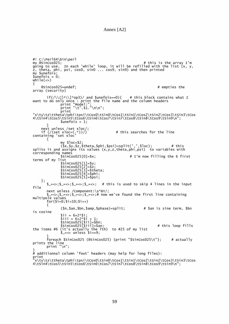
59

Annex [A2] #! C:\Perl64\bin\perl my @SinCos025; # this is the array I'm going to use. In each 'while' loop, it will be refilled with the list (x, y, z, theta, phi, psi, cos0, sin0 ... cos9, sin9) and then printed my $unefois; $unefois = 0; while(<>) { @SinCos025=undef; # empties the array (security) if(/\\([^\\]*op3)/ and $unefois==0){ # this block contains what I want to do only once : print the file name and the column headers print "Model:"; print "\t".$1."\n\n"; print "x\ty\tz\ttheta\tphi\tpsi\tCos0\tSin0\tCos1\tSin1\tCos2\tSin2\tCos3\tSin3\tCos4\tSin4\tCos5\tSin5\tCos6\tSin6\tCos7\tSin7\tCos8\tSin8\tCos9\tSin9\n"; $unefois = 1; } next unless /set xloc/; if (/(set xloc=(.*))/) # this searches for the line containing 'set xloc' { my $loc=$2; ($x,$y,$z,$theta,$phi,$psi)=split(',',$loc); # this splits it and assigns its values (x,y,z,theta,phi,psi) to variables with corresponding names $SinCos025[0]=$x; # I'm now filling the 6 first terms of my list $SinCos025[1]=$y; $SinCos025[2]=$z; $SinCos025[3]=$theta; $SinCos025[4]=$phi; $SinCos025[5]=$psi; }; $_=<>;$_=<>;$_=<>;$_=<>; # this is used to skip 4 lines in the input file next unless /Component:\s*BY/; $_=<>;$_=<>;$_=<>;$_=<>;# now we've found the first line containing multipole values for($i=0;$i<10;$i++) { ($n,$an,$bn,$amp,$phase)=split; # $an is sine term, $bn is cosine $ii = 6+2*$i; $iii = 6+2*$i + 1; $SinCos025[$ii]=$bn; $SinCos025[$iii]=$an; # this loop fills the items #6 (it's actually the 7th) to #25 of my list $_=<> unless $i==9; } foreach $SinCos025 (@SinCos025) {print "$SinCos025\t"}; # actually prints the line print "\n"; } # additionnal column 'foot' headers (may help for long files): print "x\ty\tz\ttheta\tphi\tpsi\tCos0\tSin0\tCos1\tSin1\tCos2\tSin2\tCos3\tSin3\tCos4\tSin4\tCos5\tSin5\tCos6\tSin6\tCos7\tSin7\tCos8\tSin8\tCos9\tSin9\n";

60

Annex [A3] ACTIVATE CASE=1 MODELSYMMETRY=DATABASE | LOAD

SELECT ACTION=DEFAULT | SELECT ACTION=SELECT OPTION=SURFACES |

THREED OPTION=GETVIEW | THREED OPTION=SETVIEW ROTX=-90 ROTY=0.01

ROTZ=0.01 SIZE=100 PERSPECTIVE=NO

SET FIELD=NODAL COIL=NODAL

set XLOCAL=0,YLOCAL=0,ZLOCAL=0,PLOCAL=0,TLOCAL=0,SLOCAL=0

CIRCLE RADIUS=1 TH1=0 TH2=360 ZC=0 NP=60 | PLOT FILE=TEMP COMPONENT=By

FIT TYPE=FOURIER FILE=TEMP COMP=By ORDER=10 PRINT=YES

set xloc=1.374,0.000,74.981,2.699,0.000,0.000

circ

fit

set xloc=1.362,0.000,74.731,2.690,0.000,0.000

circ

fit

set xloc=1.350,0.000,74.481,2.681,0.000,0.000

circ

fit

set xloc=1.338,0.000,74.232,2.672,0.000,0.000

circ

fit

set xloc=1.327,0.000,73.982,2.663,0.000,0.000

circ

fit

set xloc=1.315,0.000,73.732,2.654,0.000,0.000

circ

fit

set xloc=1.304,0.000,73.482,2.645,0.000,0.000

circ

fit

set xloc=1.292,0.000,73.232,2.636,0.000,0.000

circ

fit

set xloc=1.281,0.000,72.983,2.627,0.000,0.000

circ

fit

set xloc=1.269,0.000,72.733,2.618,0.000,0.000

circ

fit

set xloc=1.258,0.000,72.483,2.609,0.000,0.000

circ

fit

set xloc=1.246,0.000,72.233,2.600,0.000,0.000

circ

fit

set xloc=1.235,0.000,71.984,2.591,0.000,0.000

circ

fit

set xloc=1.224,0.000,71.734,2.582,0.000,0.000

circ

fit

set xloc=1.213,0.000,71.484,2.573,0.000,0.000

circ

fit

set xloc=1.201,0.000,71.234,2.564,0.000,0.000

circ

fit

set xloc=1.190,0.000,70.985,2.555,0.000,0.000

circ

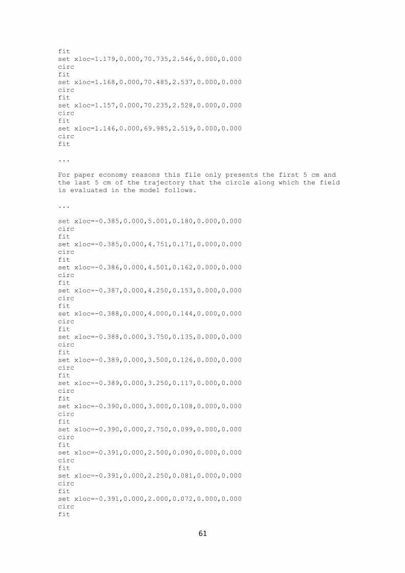
61

fit

set xloc=1.179,0.000,70.735,2.546,0.000,0.000

circ

fit

set xloc=1.168,0.000,70.485,2.537,0.000,0.000

circ

fit

set xloc=1.157,0.000,70.235,2.528,0.000,0.000

circ

fit

set xloc=1.146,0.000,69.985,2.519,0.000,0.000

circ

fit

...

For paper economy reasons this file only presents the first 5 cm and

the last 5 cm of the trajectory that the circle along which the field

is evaluated in the model follows.

...

set xloc=-0.385,0.000,5.001,0.180,0.000,0.000

circ

fit

set xloc=-0.385,0.000,4.751,0.171,0.000,0.000

circ

fit

set xloc=-0.386,0.000,4.501,0.162,0.000,0.000

circ

fit

set xloc=-0.387,0.000,4.250,0.153,0.000,0.000

circ

fit

set xloc=-0.388,0.000,4.000,0.144,0.000,0.000

circ

fit

set xloc=-0.388,0.000,3.750,0.135,0.000,0.000

circ

fit

set xloc=-0.389,0.000,3.500,0.126,0.000,0.000

circ

fit

set xloc=-0.389,0.000,3.250,0.117,0.000,0.000

circ

fit

set xloc=-0.390,0.000,3.000,0.108,0.000,0.000

circ

fit

set xloc=-0.390,0.000,2.750,0.099,0.000,0.000

circ

fit

set xloc=-0.391,0.000,2.500,0.090,0.000,0.000

circ

fit

set xloc=-0.391,0.000,2.250,0.081,0.000,0.000

circ

fit

set xloc=-0.391,0.000,2.000,0.072,0.000,0.000

circ

fit

62

set xloc=-0.392,0.000,1.750,0.063,0.000,0.000

circ

fit

set xloc=-0.392,0.000,1.500,0.054,0.000,0.000

circ

fit

set xloc=-0.392,0.000,1.250,0.045,0.000,0.000

circ

fit

set xloc=-0.392,0.000,1.000,0.036,0.000,0.000

circ

fit

set xloc=-0.392,0.000,0.750,0.027,0.000,0.000

circ

fit

set xloc=-0.392,0.000,0.500,0.018,0.000,0.000

circ

fit

set xloc=-0.393,0.000,0.250,0.009,0.000,0.000

circ

fit

set xloc=-0.393,0.000,0.000,0.000,0.000,0.000

circ

fit

end

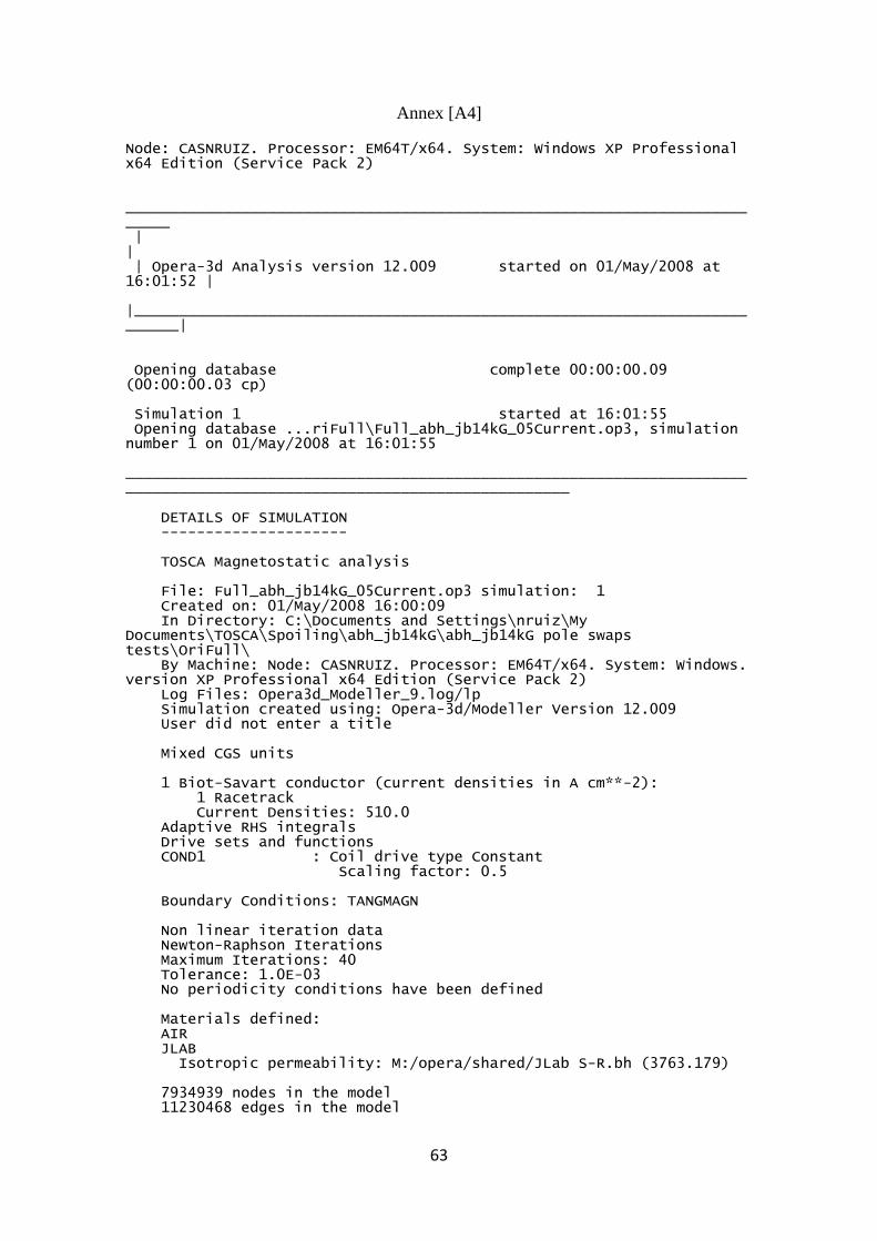
63

Annex [A4] Node: CASNRUIZ. Processor: EM64T/x64. System: Windows XP Professional x64 Edition (Service Pack 2) ___________________________________________________________________________ | | | Opera-3d Analysis version 12.009 started on 01/May/2008 at 16:01:52 | |___________________________________________________________________________| Opening database complete 00:00:00.09 (00:00:00.03 cp) Simulation 1 started at 16:01:55 Opening database ...riFull\Full_abh_jb14kG_05Current.op3, simulation number 1 on 01/May/2008 at 16:01:55 ________________________________________________________________________________________________________________________ DETAILS OF SIMULATION --------------------- TOSCA Magnetostatic analysis File: Full_abh_jb14kG_05Current.op3 simulation: 1 Created on: 01/May/2008 16:00:09 In Directory: C:\Documents and Settings\nruiz\My Documents\TOSCA\Spoiling\abh_jb14kG\abh_jb14kG pole swaps tests\OriFull\ By Machine: Node: CASNRUIZ. Processor: EM64T/x64. System: Windows. version XP Professional x64 Edition (Service Pack 2) Log Files: Opera3d_Modeller_9.log/lp Simulation created using: Opera-3d/Modeller Version 12.009 User did not enter a title Mixed CGS units 1 Biot-Savart conductor (current densities in A cm**-2): 1 Racetrack Current Densities: 510.0 Adaptive RHS integrals Drive sets and functions COND1 : Coil drive type Constant Scaling factor: 0.5 Boundary Conditions: TANGMAGN Non linear iteration data Newton-Raphson Iterations Maximum Iterations: 40 Tolerance: 1.0E-03 No periodicity conditions have been defined Materials defined: AIR JLAB Isotropic permeability: M:/opera/shared/JLab S-R.bh (3763.179) 7934939 nodes in the model 11230468 edges in the model

64

Mixed linear and quadratic tetrahedral elements 4275047 linear tetrahedra 5346565 quadratic tetrahedra ________________________________________________________________________________________________________________________ Loading problem description complete 00:00:16.18 (00:00:14.60 cp) Setting scalar potential to 0 at node 1 at (-17.13297,149.56413,0.0 ) [cm] Checking periodicity transformations Checking connectivity of potential regions: 2 automatic potential cuts have been added. Preparing data complete 00:04:14.63 (00:04:08.15 cp) Problem size information ------------------------ Number of elements : 9621612 Number of nodes : 7934939 Number of equations : 7752319 Number of non-zeros : 109689916 Forming Matrix Sparsity complete 00:01:33.82 (00:01:21.14 cp) Selecting coil field calculations complete 00:00:37.29 (00:00:37.04 cp) Coil set with drive label COND1 Calculating coil fields at 947415 nodes Coil fields computed at 94741 nodes Coil fields computed at 189482 nodes Coil fields computed at 284223 nodes Coil fields computed at 378964 nodes Coil fields computed at 473705 nodes Coil fields computed at 568446 nodes Coil fields computed at 663187 nodes Coil fields computed at 757928 nodes Coil fields computed at 852669 nodes Coil fields computed at 947410 nodes Calculating nodal coil fields complete 00:06:21.78 (00:06:16.29 cp) Coil set with drive label COND1 Calculating line integrals along 140939 edges Coil field line integrals computed along 14093 edges Coil field line integrals computed along 28186 edges Coil field line integrals computed along 42279 edges Coil field line integrals computed along 56372 edges Coil field line integrals computed along 70465 edges Coil field line integrals computed along 84558 edges Coil field line integrals computed along 98651 edges Coil field line integrals computed along 112744 edges Coil field line integrals computed along 126837 edges Coil field line integrals computed along 140930 edges Total number of field calculations: 318231 Average number of field calculations per edge: 2.2579 Calculating edge integral coil fields complete 00:01:57.89 (00:01:56.14 cp) Coil set with drive label COND1 DSLUCG iterations: 1614 Relative change= 0.99230E-12 Error in nodal potential jump calculation: 1.3506E-05% Calculating nodal potential jump values complete 00:01:52.98 (00:01:51.35 cp) Coil set with drive label COND1 Calculating face integrals of Nodal WH.n over 121642 faces Coil field integrals computed over 12164 faces

65

Coil field integrals computed over 24328 faces Coil field integrals computed over 36492 faces Coil field integrals computed over 48656 faces Coil field integrals computed over 60820 faces Coil field integrals computed over 72984 faces Coil field integrals computed over 85148 faces Coil field integrals computed over 97312 faces Coil field integrals computed over 109476 faces Coil field integrals computed over 121640 faces Total number of field calculations: 851494 Average number of field calculations per face: 7.0 Calculating face integral coil fields complete 00:05:23.00 (00:05:18.14 cp) Evaluating coil field calculations complete 00:15:45.51 (00:15:31.67 cp) Initial residual: 51325575. Nonlinear iteration 1 started at 16:29:13 Simple nonlinear update DSLUCG iterations: 1071 Relative change= 0.99336E-08 Iterative matrix solution complete 00:53:46.51 (00:52:21.56 cp) Residual: 918.042188, relaxation factor: 1.0 Relaxing solution change complete 00:02:46.46 (00:02:38.42 cp) Nonlinear iteration 1 complete 00:56:34.96 (00:55:01.96 cp) Nonlinear iteration 2 started at 17:25:48 Newton-Raphson nonlinear update DSLUCG iterations: 499 Relative change= 0.51251E-06 Iterative matrix solution complete 00:27:10.12 (00:26:30.60 cp) Residual: 1161.05011, relaxation factor: 0.0625 Convergence indicators (Changes): 1.188E-03, 0.7129258 (target 1.0E-03 ) Relaxing solution change complete 00:13:31.27 (00:13:10.15 cp) Nonlinear iteration 2 complete 00:43:40.33 (00:42:36.01 cp) Nonlinear iteration 3 started at 18:09:29 Simple nonlinear update DSLUCG iterations: 375 Relative change= 0.94291E-08 Iterative matrix solution complete 00:18:02.80 (00:17:34.84 cp) Residual: 1216.13381, relaxation factor: 0.0625 Convergence indicators (Changes): 6.653E-04, 0.1579107 (target 1.0E-03 ) Relaxing solution change complete 00:18:28.10 (00:18:00.89 cp) Nonlinear iteration 3 complete 00:36:32.87 (00:35:37.68 cp) Nonlinear iteration 4 started at 18:46:02 Newton-Raphson nonlinear update Jacobian terms relaxed 0.25 DSLUCG iterations: 459 Relative change= 0.54109E-06 Iterative matrix solution complete 00:24:50.53 (00:24:14.12 cp) Residual: 1288.01111, relaxation factor: 0.0625 Convergence indicators (Changes): 7.163E-04, 0.2656289 (target 1.0E-03 ) Relaxing solution change complete 00:18:27.83 (00:17:51.71 cp) Nonlinear iteration 4 complete 00:45:49.11 (00:44:33.56 cp) Nonlinear iteration 5 started at 19:31:51

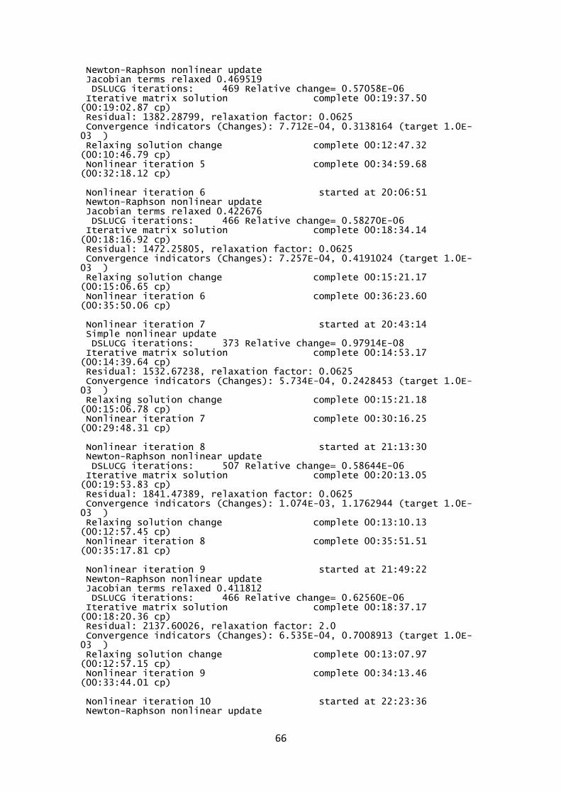
66

Newton-Raphson nonlinear update Jacobian terms relaxed 0.469519 DSLUCG iterations: 469 Relative change= 0.57058E-06 Iterative matrix solution complete 00:19:37.50 (00:19:02.87 cp) Residual: 1382.28799, relaxation factor: 0.0625 Convergence indicators (Changes): 7.712E-04, 0.3138164 (target 1.0E-03 ) Relaxing solution change complete 00:12:47.32 (00:10:46.79 cp) Nonlinear iteration 5 complete 00:34:59.68 (00:32:18.12 cp) Nonlinear iteration 6 started at 20:06:51 Newton-Raphson nonlinear update Jacobian terms relaxed 0.422676 DSLUCG iterations: 466 Relative change= 0.58270E-06 Iterative matrix solution complete 00:18:34.14 (00:18:16.92 cp) Residual: 1472.25805, relaxation factor: 0.0625 Convergence indicators (Changes): 7.257E-04, 0.4191024 (target 1.0E-03 ) Relaxing solution change complete 00:15:21.17 (00:15:06.65 cp) Nonlinear iteration 6 complete 00:36:23.60 (00:35:50.06 cp) Nonlinear iteration 7 started at 20:43:14 Simple nonlinear update DSLUCG iterations: 373 Relative change= 0.97914E-08 Iterative matrix solution complete 00:14:53.17 (00:14:39.64 cp) Residual: 1532.67238, relaxation factor: 0.0625 Convergence indicators (Changes): 5.734E-04, 0.2428453 (target 1.0E-03 ) Relaxing solution change complete 00:15:21.18 (00:15:06.78 cp) Nonlinear iteration 7 complete 00:30:16.25 (00:29:48.31 cp) Nonlinear iteration 8 started at 21:13:30 Newton-Raphson nonlinear update DSLUCG iterations: 507 Relative change= 0.58644E-06 Iterative matrix solution complete 00:20:13.05 (00:19:53.83 cp) Residual: 1841.47389, relaxation factor: 0.0625 Convergence indicators (Changes): 1.074E-03, 1.1762944 (target 1.0E-03 ) Relaxing solution change complete 00:13:10.13 (00:12:57.45 cp) Nonlinear iteration 8 complete 00:35:51.51 (00:35:17.81 cp) Nonlinear iteration 9 started at 21:49:22 Newton-Raphson nonlinear update Jacobian terms relaxed 0.411812 DSLUCG iterations: 466 Relative change= 0.62560E-06 Iterative matrix solution complete 00:18:37.17 (00:18:20.36 cp) Residual: 2137.60026, relaxation factor: 2.0 Convergence indicators (Changes): 6.535E-04, 0.7008913 (target 1.0E-03 ) Relaxing solution change complete 00:13:07.97 (00:12:57.15 cp) Nonlinear iteration 9 complete 00:34:13.46 (00:33:44.01 cp) Nonlinear iteration 10 started at 22:23:36 Newton-Raphson nonlinear update

67

Jacobian terms relaxed 0.661812 DSLUCG iterations: 955 Relative change= 0.84330E-06 Iterative matrix solution complete 00:37:53.64 (00:37:20.73 cp) Residual: 2166.07792, relaxation factor: 0.0625 Convergence indicators (Changes): 3.337E-04, 1.0089306 (target 1.0E-03 ) Relaxing solution change complete 00:21:55.24 (00:21:35.42 cp) Nonlinear iteration 10 complete 01:02:18.97 (01:01:22.66 cp) Nonlinear iteration 11 started at 23:25:55 Newton-Raphson nonlinear update Jacobian terms relaxed 0.912046 DSLUCG iterations: 1028 Relative change= 0.85639E-06 Iterative matrix solution complete 00:40:51.46 (00:40:14.18 cp) Residual: 2287.02397, relaxation factor: 2.0 Convergence indicators (Changes): 5.793E-04, 1.8099201 (target 1.0E-03 ) Relaxing solution change complete 00:13:08.50 (00:12:57.60 cp) Nonlinear iteration 11 complete 00:56:30.22 (00:55:38.41 cp) Nonlinear iteration 12 started at 00:22:25 Newton-Raphson nonlinear update Jacobian terms relaxed 0.897612 DSLUCG iterations: 1042 Relative change= 0.11989E-05 Iterative matrix solution complete 00:41:22.56 (00:40:44.11 cp) Residual: 848.204579, relaxation factor: 1.0 Convergence indicators (Changes): 7.087E-04, 0.585946 (target 1.0E-03 ) Relaxing solution change complete 00:02:11.53 (00:02:09.73 cp) Nonlinear iteration 12 complete 00:46:02.47 (00:45:20.40 cp) Nonlinear iteration 13 started at 01:08:27 Newton-Raphson nonlinear update DSLUCG iterations: 491 Relative change= 0.45054E-05 Iterative matrix solution complete 00:19:34.78 (00:19:16.14 cp) Residual: 180.909221, relaxation factor: 1.0 Convergence indicators (Changes): 3.971E-04, 0.7704239 (target 1.0E-03 ) Relaxing solution change complete 00:02:11.56 (00:02:09.76 cp) Nonlinear iteration 13 complete 00:24:14.69 (00:23:52.45 cp) Nonlinear iteration 14 started at 01:32:42 Newton-Raphson nonlinear update DSLUCG iterations: 412 Relative change= 0.18134E-04 Iterative matrix solution complete 00:16:26.10 (00:16:11.29 cp) Residual: 12.749083 , relaxation factor: 1.0 Convergence indicators (Changes): 2.829E-05, 0.0614732 (target 1.0E-03 ) Relaxing solution change complete 00:02:11.53 (00:02:09.71 cp) Nonlinear iteration 14 complete 00:21:05.97 (00:20:47.56 cp) Nonlinear iteration 15 started at 01:53:48 Newton-Raphson nonlinear update DSLUCG iterations: 382 Relative change= 0.99830E-04

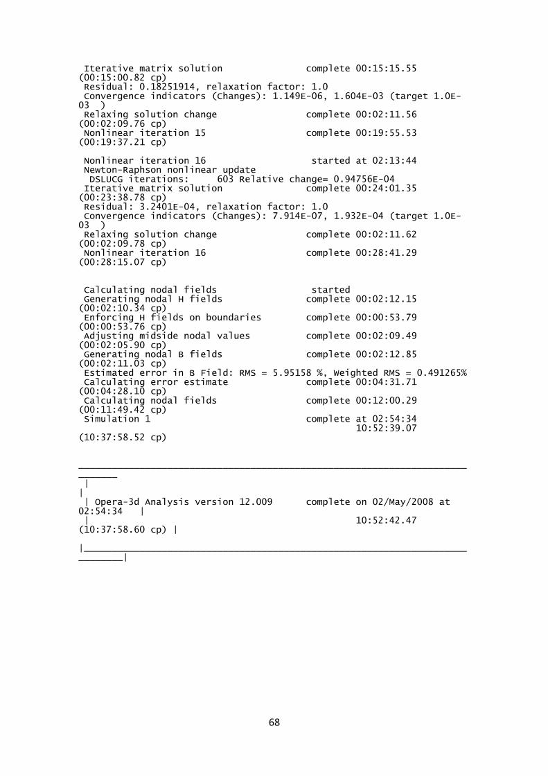
68

Iterative matrix solution complete 00:15:15.55 (00:15:00.82 cp) Residual: 0.18251914, relaxation factor: 1.0 Convergence indicators (Changes): 1.149E-06, 1.604E-03 (target 1.0E-03 ) Relaxing solution change complete 00:02:11.56 (00:02:09.76 cp) Nonlinear iteration 15 complete 00:19:55.53 (00:19:37.21 cp) Nonlinear iteration 16 started at 02:13:44 Newton-Raphson nonlinear update DSLUCG iterations: 603 Relative change= 0.94756E-04 Iterative matrix solution complete 00:24:01.35 (00:23:38.78 cp) Residual: 3.2401E-04, relaxation factor: 1.0 Convergence indicators (Changes): 7.914E-07, 1.932E-04 (target 1.0E-03 ) Relaxing solution change complete 00:02:11.62 (00:02:09.78 cp) Nonlinear iteration 16 complete 00:28:41.29 (00:28:15.07 cp) Calculating nodal fields started Generating nodal H fields complete 00:02:12.15 (00:02:10.34 cp) Enforcing H fields on boundaries complete 00:00:53.79 (00:00:53.76 cp) Adjusting midside nodal values complete 00:02:09.49 (00:02:05.90 cp) Generating nodal B fields complete 00:02:12.85 (00:02:11.03 cp) Estimated error in B Field: RMS = 5.95158 %, Weighted RMS = 0.491265% Calculating error estimate complete 00:04:31.71 (00:04:28.10 cp) Calculating nodal fields complete 00:12:00.29 (00:11:49.42 cp) Simulation 1 complete at 02:54:34 10:52:39.07 (10:37:58.52 cp) _____________________________________________________________________________ | | | Opera-3d Analysis version 12.009 complete on 02/May/2008 at 02:54:34 | | 10:52:42.47 (10:37:58.60 cp) | |_____________________________________________________________________________|