determination of the effect of stress state on the onset

Determination of the Effect of Stress State on the Onsetof Ductile Fracture Through Tension-Torsion Experiments

The MIT Faculty has made this article openly available. Please share how this access benefits you. Your story matters.

Citation Papasidero, J., V. Doquet, and D. Mohr. “Determination of theEffect of Stress State on the Onset of Ductile Fracture ThroughTension-Torsion Experiments.” Experimental Mechanics 54, no. 2(September 7, 2013): 137–151.

As Published http://dx.doi.org/10.1007/s11340-013-9788-4

Publisher Springer US

Version Author's final manuscript

Citable link http://hdl.handle.net/1721.1/103339

Terms of Use Article is made available in accordance with the publisher'spolicy and may be subject to US copyright law. Please refer to thepublisher's site for terms of use.

https://libraries.mit.edu/forms/dspace-oa-articles.html

http://hdl.handle.net/1721.1/103339

Determination of the Effect of Stress State on the Onset of

Ductile Fracture Through Tension-Torsion Experiments

Jessica Papasidero1,Véronique Doquet1 and Dirk Mohr1,2

1Solid Mechanics Laboratory (CNRS-UMR 7649), Department of Mechanics,

École Polytechnique, Palaiseau, France 2Impact and Crashworthiness Laboratory, Department of Mechanical Engineering,

Massachusetts Institute of Technology, Cambridge MA, USA

Abstract. A tubular tension-torsion specimen is proposed to characterize the onset of

ductile fracture in bulk materials at low stress triaxialities. The specimen features a

stocky gage section of reduced thickness. The specimen geometry is optimized such that

the stress and strain fields within the gage section are approximately uniform prior to

necking. The stress state is plane stress while the circumferential strain is approximately

zero. By applying different combinations of tension and torsion, the material response

can be determined for stress triaxialities ranging from zero (pure shear) to about 0.58

(transverse plane strain tension), and Lode angle parameters ranging from 0 to 1. The

relative displacement and rotation of the specimen shoulders as well as the surface strain

fields within the gage section are determined through stereo digital image correlation.

Multi-axial fracture experiments are performed on a 36NiCrMo16 high strength steel. A

finite element model is built to determine the evolution of the local stress and strain fields

all the way to fracture. Furthermore, the newly-proposed Hosford-Coulomb fracture

initiation model is used to describe the effect of stress state on the onset of fracture.

Keywords: Ductile fracture, stress triaxiality, Lode angle, combined loading, torsion

Papasidero et al., revised version (May 23, 2013)

2

1. Introduction

Recent research on ductile fracture emphasizes the effect of the third stress invariant

on the onset of ductile fracture in metals. Examples include the recent studies by

Barsoum and Faleskog (2007), Nahshon and Hutchinson (2009), Bai and Wierzbicki

(2010) and Nielsen and Tvergaard (2011) which all hypothesize on the dependence of the

equivalent plastic strain to fracture on the third stress tensor invariant in addition to the

stress triaxiality. Micromechanical demonstrations of the effect of the Lode parameter

have been presented among others by Barsoum and Faleskog (2007), Danas and Ponte

Castaneda (2012) and Dunand and Mohr (2013).

At this stage, it is still very difficult to draw concrete conclusions on the effect of the

Lode angle on the onset of fracture based on experiments. Reliable experiments

characterizing the effect of stress state on the onset of ductile fracture are difficult to

achieve, in particular due to necking prior to the onset of fracture in thin-walled

specimens. Hybrid experimental-numerical techniques have been developed to address

this issue. Mohr and Henn (2007) subjected flat butterfly-shaped specimens to combined

tension and shear loading. Due to the heterogeneity of the stress and strain fields in the

specimen gage section, they made use of a finite element model to determine the stress

and strain histories at the location of fracture initiation. This technique has been

developed further by Teng et al. (2009) and Dunand and Mohr (2011) by optimizing the

specimen shape to reduce experimental errors, and through the use of more advanced

plasticity models for the identification of the loading path to fracture. In the case of sheet

materials, the butterfly testing technique requires a local reduction of the initial specimen

thickness. This machining procedure may affect the mechanical properties of the


3

specimen material (see Mohr and Ebnoether, 2009) which adds to the uncertainty in the

experimental results. Flat notched specimens provide a robust alternative to this

technique to characterize the fracture response at stress triaxialities above 0.33. It is now

common practice to take a hybrid experimental-numerical approach to analyze notched

tensile experiments (e.g. Dunand and Mohr, 2010). Similarly, other sheet specimen

geometries are being used to cover different stress states. The maturation of digital image

correlation techniques (e.g. Bornert et al., 2009, Sutton et al., 2009) also contributed

significantly to the success of hybrid experimental-numerical approaches.

In the case of bulk materials, tubular specimens can be extracted to perform

combined tension-torsion experiments. The first experiments of this type have been

performed already one century ago. The most prominent are those by Taylor and Quinney

(1932) which were instrumental in the development of multi-axial plasticity models of

metals. Taylor and Quinney (1932) used rather slender thick-walled tubes, while more

stocky thin-walled tubes are used today. For example, Nouailhas and Cailletaud (1995)

used 1mm thick tubes with an inner diameter of 14mm and a free length of 24mm to

investigate the tension-torsion response of single crystal superalloys. Zhang and Jiang

(2005) studied the propagation of Lüders bands in 1045 steel using a 1.1mm thick

tension-torsion specimen of an inner diameter of 20.2mm and a gage section length of

25.4mm. Khan et al. (2009, 2010) used a tubular specimen of 12.7mm inner diameter

with a 50.8mm long, 1.4mm thick gage section to perform tension-torsion experiments on

Al6061-T6511 and annealed Al-1100.

Multi-axial stress states in tubular specimens may also be achieved through

combinations of tension and internal pressure. While the above experimentalists used


4

tension-torsion experiments for plasticity characterization, tension-internal pressure

experiments have been performed to study both the plasticity and ductile fracture of

metals. For example, Kuwabara et al. (2005) tested Al 5154-H112 tubes of 76.3mm outer

diameter and 3.9mm wall thickness under tension and internal pressure. Korkolis et al.

(2010) subjected Al-6061-T6 tubes to internal pressure and axial load to investigate the

plasticity and fracture under biaxial loading. Their specimens featured a nominal

diameter of 51mm, a wall thickness of 1.65mm and a test section length of 229mm.

Shear buckling often limits the validity of tension-torsion experiments to moderate

strains. In order to test engineering materials all the way to fracture under combined

tension-torsion loading, Barsoum and Faleskog (2007) introduced a symmetric

circumferential notch into the tube wall, thereby concentrating plastic deformation into a

very narrow region. To investigate the ductile fracture of Weldox steels, they used a

nominal specimen diameter of 24mm, a wall thickness of 1.2mm within the notched

section and of 3.2mm outside the notch. The notch radius was only 0.5mm, which creates

substantial radial stresses when tension is applied. Their experimental program covered

stress triaxialities (at the onset of fracture) from about 0.3 to 1.2. Another strategy for

preventing shear buckling is to shorten the specimen gage section. This approach has no

obvious negative effect when applying torsion only, but it changes the stress state in

tension. For pure tension applied to the specimen boundaries, the stress state in the tube

walls is no longer uni-axial tension, but close to transverse plane strain tension instead, as

circumferential deformation is prohibited by the boundary conditions in stocky tension-

torsion specimens.


5

Short tubular specimens are commonly used for dynamic torsion testing of metals.

For example, Lindholm et al. (1980) employed a specimen of an inner diameter of

12.9mm, a gage section length of 3.1mm and a gage section thickness of 0.8mm. Note

that the choice of a very short gage section in a specimen for dynamic testing is not only

driven by stability considerations, but also necessary to ensure locally quasi-static loading

conditions. Gao et al. (2011) modified a dynamic torsion specimen to perform static

fracture experiments on Al 5053-H116 (extracted from plate stock). The specimen gage

section was 2.5mm long and 0.75mm thick. The tube inner diameter was 13.1mm, the

outer diameter 25.4mm. In a follow-up paper, Graham et al. (2012) show that this

experimental technique covers a range of stress triaxiality from 0 to 0.6. A very recent

study on the ductile failure of aluminum 60161-T6 under combined tension and shear has

been completed by Haltom et al. (2013). They used a tubular specimen of a uniform inner

diameter of 44.3mm and a wall thickness of 1mm within the 10mm long test section.

In this paper, a stocky tubular specimen is presented for characterizing the onset of

fracture in bulk materials at low stress triaxialities. Combined tension-torsion fracture

experiments are performed on an initially isotropic high strength steel. Using a hybrid

numerical-experimental procedure, the loading paths up to the onset of fracture are

determined and presented in the space of stress triaxiality, Lode angle parameter and

equivalent plastic strain. These results are subsequently used to identify the parameters of

the Hosford-Coulomb fracture initiation model.


6

2. Specimen design

2.1. Specimen geometry

Figure 1 shows a sketch of the axisymmetric specimen geometry proposed for the

testing of metals under combined tension and torsion. The specimen geometry is

characterized by five parameters (Fig. 1b): the inner diameter D , the gage section

thickness t , the gage section height h , the wall thickness e of the shoulder region, and

the fillet radius a (Fig. 1b). The main considerations in specifying the specimen

dimensions are:

(1) the maximum axial force and torque may not exceed 100kN and 600Nm,

respectively; this limitation along with the availability of suitable specimen

clamps led to the choice of D=20mm.

(2) the thickness-to-diameter ratio, Dt / , needs to be small to reduce the gradients in

the stress and strain fields along the radial direction; a minimum thickness of

t=1mm is chosen in view of uncertainties in the experimental results associated

with dimensional inaccuracies in the initial specimen geometry (for example, a

machining tolerance of mµ50± equates to an uncertainty of 5% in the reported

average stress fields)

(3) the shoulder-to-gage section thickness ratio, te / , needs to be sufficiently large to

prevent the plastic deformation of the shoulder region; a shoulder thickness of

mme 2= is chosen to prevent the plastic deformation of the shoulders even for

high strain hardening materials.


7

(4) the height-to-thickness ratio, th / , needs to be small to prevent buckling under

torsion;

In addition, the results from a finite element study revealed that

(5) the greater the height-to-thickness ratio, th / , the smaller the radial gradient in

stress triaxiality (Fig. 2a). Based on (4) and (5), a gage section height of

mmh 2= is chosen.

(6) The greater the fillet radius a , the more uniform the stress fields. However, a

should be small to keep the effective buckling length short. We chose a radius of

mma 1= ; for this radius, there is no noticeable notch effect when tension is

applied to the specimen, i.e. the radial stresses are still negligibly small as

compared to the axial and circumferential stress components (Fig. 2b).

Figure 5c provides a summary of the final gage section and shoulder dimensions.

2.2. Analytical estimate of the achievable stress states

Given the stockiness of the specimen gage section, the achievable stress states are

computed assuming zero plastic circumferential strain. Furthermore, plane stress

conditions (along the radial direction) are assumed. For a Levy-von Mises material, the

flow rule yields

zzσσθθ 5.0= . (1)

The Cauchy stress tensor may thus be written as


8

)(5.0 ZZZZ eeeeeeeeσ ⊗+⊗+⊗+⊗= ΘΘΘΘ τσσ (2)

where σ denotes the stress along the Ze -direction, and τ is the shear stress in the

),( ΘeeZ -plane.

The stress state is characterized through the stress triaxiality and the Lode angle

parameter. The stress triaxiality η is defined by the ratio of the hydrostatic stress and the

von Mises stress,

σση m= (3)

with 3)(σtrm =σ , ss :23=σ and 1σs mσ−= . The Lode angle parameter θ depends

on the normalized third invariant of the deviatoric stress tensor,

−=3

)det(

2

27cos

21

σπθ s

a . (4)

Due to this particular definition, the Lode angle parameter is bound between -1 and 1.

The stress state in the specimen gage section is controlled by the ratio of torsion and axial

loading. Based on the specimen diameterD , the axial force F and the torque M , the

biaxial loading angle β is defined as

τσβ ≅=

M

FD

2tan . (5)

Combining Eqs. (2), (3) and (4), the stress triaxiality and the Lode angle parameter can be

expressed in terms of the biaxial loading angle,


9

4tan

tan

3

12 +

=ββη

(6)

. (7)

The Lode angle parameter is plotted as a function of the stress triaxiality in Fig. 3, while

β is used as curve parameter. Note that this relationship between the Lode angle and the

stress triaxiality is only valid for plane stress conditions. For °=0β (torsion only), the

stress state corresponds to pure shear which is characterized by 0=η and 0=θ . The

same Lode angle parameter value is achieved for °=90β (tension only) where the stress

state corresponds to transverse plane strain tension. A uniaxial stress state ( 33.0=η and

1=θ ) prevails for combined tension-torsion loading at °≅55β .

3. Experiments

3.1. Material

All specimens are extracted from an annealed 30mm diameter bar of the high

strength steel 36NiCrMo16. Table 1 shows the chemical composition as provided by the

manufacturer ThyssenKrupp. Microscopic analysis after etching with a Villela solution

revealed a tempered martensitic structure (Fig. 4). Large strain compression tests on

13mm-large cubes extracted along the bar axis and the transverse direction revealed no

noticeable anisotropy in the material behavior at the macroscopic level.

( )

+−= 232 4tan

tan36cos

21

ββ

πθ a


10

3.2. Experimental procedure

A servo-hydraulic axial/torsion and internal pressure loading frame (TEMA Concept,

France) is used to perform all experiments (Fig. 5a). The vertical and rotational actuators

cover a range of ±100kN and ±600Nm, respectively. Throughout the experiments, the

biaxial loading angle is kept constant using different control settings (Tab 2):

• For °= 0β , the rate of rotation is prescribed, while operating the vertical actuator

under force control ( 0=F ).

• For °<< 550 β (shear-dominated), the rotation is prescribed, while the axial

position is incrementally adjusted such that β remains constant.

• For °<≤° 9055 β (tension-dominated), the axial displacement is prescribed,

while the rotation is incrementally adjusted such that β remains constant.

• For °= 90β , the axial velocity is prescribed, while operating the rotational

actuator under torque control ( 0=M ).

3.3. Displacement and strain measurement

The displacement fields within the gage section and a part of the shoulder regions are

measured using stereo Digital Image Correlation (DIC). A thin layer of matt white paint

is applied onto the specimen surface along with a black speckle pattern. Two digital

cameras (Pike F505B 2452x2054 with 90mm Tamron macro lenses) are used to take

about 200 pictures throughout each experiment. The camera sensors are positioned at a

distance of about 0.80m from the specimen surface with an F11 aperture to ensure


11

sufficient depth of field for measuring large rotations. The relative position of the

cameras and the respective focal lengths are identified from preliminary measurements

on a rigid target. The displacement field is computed based on the acquired images using

the VIC3D software (Correlated Solutions) assuming an affine transformation of a 21x21

pixel subset (with 24 mµ per pixel).

Based on the measured initial shape, a cylindrical coordinate system ),,( ZR eee Θ is

established such that the Ze -vector coincides with the specimen axis (Fig. 1b). The

initial position of a point on the specimen surface is then given by the position vector

ZR ZR eeX +Θ= ][ , (8)

while its current position on the deformed specimen surface reads

ZR zr eex += ][θ . (9)

The functions

],,[ ZRrr Θ= (10)

],,[ ZR Θ=θθ (11)

],,[ ZRzz Θ= (12)

are obtained from stereo digital image correlation.

The DIC position measurements serve two purposes. Firstly, the relative motion of

two points A and B positioned on the respective upper and lower specimen shoulder (Fig.

5b) is determined,


12

)()()( tztztU BA −=∆ , (13)

)()()( ttt BA θθθ −=∆ . (14)

Secondly, the surface strain field is computed from the position measurements. Re-

writing the vector of the current position in terms of the base vectors associated with the

initial configuration,

ZzRR xxx eeex +Θ+Θ= ΘΘ ][][ , (15)

with

( )Θ−= θcosrxR , ]sin[ Θ−=Θ θrx and zxZ = , (16)

the surface deformation gradient is given as

∂∂

Θ∂∂

∂∂

+Θ∂

∂

=ΘΘ

Z

xx

R

Z

xx

x

RZZ

R

1

1

F . (17)

The nominal strain tensor is then computed as

1FFε −+= )(21 T (18)

after verifying that 0/ ≅Θ∂∂ Zx holds true for all measured deformation fields. In an

attempt to compensate for fluctuations in the strain field due to the polycrystalline nature

of the microstructure (and the noise in the DIC measurements), we report the spatial

average of the surface strain fields over a square area of mA µ200200×= ,

∫

=>=<

A z

dZA εγ

γεθ

2/

2/1εε . (19)


13

In the sequel, the components θε , zε and γ of this average nominal strain tensor are

referred to as circumferential, axial and shear strain, respectively.

In addition to the nominal strains, we also evaluate the average logarithmic surface

strain tensor >< lnε . For this, F is decomposed into a rotation R and the right stretch

tensor,

∑=

⊗==2

1iiii

T uuFRU λ (20)

which yields

∑=

⊗=2

1ln )ln(

iiii uuε λ . (21)

3.4. Average Cauchy stress estimates

Throughout the experiments, the axial force F and the torque M are measured.

Neglecting the radial gradient in the mechanical fields within a cross-section, the average

true axial stress σ and the average true shear stress τ can be estimated,

)1()( zttD

F επ

σ ++

= . (22)

and (using Bredt’s approximation)

θεε

πτ

++

+=

1

1

)(

22

z

ttD

M, (23)

with D and t denoting the initial inner diameter and initial thickness, respectively.


14

3.5. Experimental results

3.5.1 Overview

Experiments are performed for five distinct biaxial loading angles: °=0β , °= 1.34β ,

°=55β , °= 5.69β and °=90β . As illustrated in Fig. 3, °=0β corresponds approximately

to pure shear, °=55β to uniaxial tension, and °=90β to transverse plane strain tension.

The experiments for the intermediate loading angles °= 1.34β and °= 5.69β feature

approximately the same Lode angle parameter )54.0( =θ , but two distinct stress

triaxialities ( 18.0=η and 49.0=η ).

The measured force-displacement curves ( uF ∆− ) and moment-rotation curves

)( θ∆−M are shown as dashed lines in Fig. 6. The end of each dashed curve corresponds

to the point where a sudden drop in force/torque occurs. At this instant, a macroscopic

crack becomes visible on the specimen surface (specimen fracture). A monotonically

increasing moment-rotation curve is measured for pure torsion ( °=0β ). In all

experiments with tension applied, we observe a modest decrease in the axial force-

displacement curve prior to specimen fracture. At the macroscopic level, it is interesting

to observe that a higher axial displacement can be achieved when applying torsion in

addition to tension (compare uF ∆− curve for °= 5.69β with that for °=90β ).

The loading paths in terms of the measured nominal surface strains are shown in

Figs. 7a and 7b. The maximum shear strain under pure torsion is 55.1=γ , while a

maximum axial strain of 45.0=zε is observed for °=69β . The plot of the evolution of


15

the circumferential strain (Fig. 7b) reveals that the assumption of plane strain conditions

along the circumference is not full-filled in reality. According to the stereo DIC

measurement, the magnitude of the circumferential strain (contraction) is about 10% of

the axial strain. The loading paths in terms of the average true shear and axial stresses

(Fig. 7c) are approximately linear which is an immediate consequence of keeping the

loading angle β constant throughout loading. From a theoretical point of view, the non-

linearity in the average true stress loading paths is only due to the non-zero

circumferential strain (see Eqs. (22) and (23)).

3.5.2 Surface strain fields and localization

Selected strain fields just prior to the onset of fracture are shown in Fig. 8 next to the

photographs of the fractured specimens. The contour maps demonstrate the uniformity of

the strain field along the circumference up to fracture initiation. For °=90β , the final

crack is located near the plane 0=Z which is attributed to the localization of plastic

deformation at the specimen center. The same observation and argument hold also true

for °=55β (Figs. 8c and 8d). However, the final crack meanders along the circumference

for °=0β (Fig. 8e), where the strain field remains more or less uniform up to the onset of

fracture (Fig. 8f).

To shed some light on the localization of deformation prior to specimen fracture, we

extracted the distribution of selected components of the logarithmic surface strain tensor

along the z-axis from the digital image correlation results (Fig. 9):


16

• Figures 9a to 9c summarize the results for °=90β . At force maximum (point

① in Fig. 9a) and slightly beyond (point ②), the distribution of lnzzε along

the z-axis is approximately uniform. Note that we plotted the unfiltered strain

distribution (dashed lines) along with that obtained after applying a moving

spatial average filter on a 200µm kernel (solid line). When the strain exceeds

about 0.15, the strains tend to localize within an about mm1 long region of

the gage section (necking). This observation is consistent with the cross-

sectional view of the fractured specimen (Fig. 9c) which shows a pronounced

through-thickness neck.

• For tension-torsion loading at °=55β (Figs. 9d to 9f), the localization of

plastic deformation occurs at a surface strain of about 2.0ln ≅zzε . The zone of

plastic localization is only about mm5.0 wide and therefore more narrow

than for °=90β . A maximum surface strain of about 5.0ln ≅zzε is reached

prior to specimen fracture, which is twice as high as that for °=90β .

• For °=0β (pure shear), the variation of the shear component lnzθε of the

logarithmic strain tensor is plotted as a function of Z (Figs. 9g to 9j). The

plots at different stages of loading show a more or less uniform distribution

at all stages of loading. Specimen fracture occurs at a surface strain of about

58.0ln =zθε . Unlike for °=55β and °90 , The corresponding fracture surface

is not inclined, but perpendicular to the Ze -axis.


17

4. Finite element analysis

Necking prior to the onset of fracture appears to be unavoidable for biaxial loading

angles greater than °55 (except for low ductility, high strain hardening materials). As a

result, the mechanical fields exhibit significant variations along the radial directions. In

order to obtain accurate estimates of the stress and strain fields inside the specimen, a

finite element analysis of each experiment is performed.

4.1. Finite element model

The specimen geometry is discretized with four-node axisymmetric elements with a

twist degree of freedom (type CGAX4R of the Abaqus/standard element library, Abaqus,

2011). Based on a mesh size convergence study with respect to the evolution of the

equivalent plastic strain in the specimen center, the specimen gage section is discretized

with 40 first-order elements along the radial direction (Fig. 1b). The degrees of freedom

of the nodes on the top surface are all coupled in a virtual rigid body via one reference

node on the axis of rotation (node N1 in Fig. 1b). Similarly, the degrees of freedom of the

nodes on the bottom surface are coupled to those of the reference node N2. All

displacements and rotations are set to zero for the latter. A tension (respectively torsion)

test is simulated by applying an axial displacement (respectively rotation) on the

reference node N1, as measured by DIC. For combined loading, a user subroutine

(UAMP) is employed to mimic the experimental procedure: for °≥55β , the axial

displacement is prescribed and the rotation history is incrementally adjusted such that β

remained constant. Analogously, for °<55β , the rotation is prescribed while the axial


18

displacement is adjusted incrementally. At least 100 implicit time steps are performed to

complete a simulation.

4.2. Constitutive equations

A basic J2-plasticity model is used to describe the elasto-plastic response of the

material in an approximate manner. The isotropic yield function is expressed in terms of

the equivalent von Mises stress ][σσσ = and a deformation resistance ][ pkk ε= ,

0][][] ,[ =−= pp kf εσε σσ . (24)

Furthermore, an associated flow rule is assumed,

σε

∂∂= σε )( p

p dd . (25)

with pdε defining the increment in the equivalent plastic strain. Only monotonic loading

paths are considered and we thus limit our attention to a simple isotropic hardening

model. Following the work of Sung et al. (2010) and Mohr and Marcadet (2013), a

combined Voce-Swift model is used,

( ) np

bp AeQkdkk p )(1][ 00 εεε ε ++−+== −

(26)

with the Swift parameters },,{ 0 nA ε and the Voce parameters },,{ 0 bQk .


19

4.3. Identification of the plasticity model parameters

The isotropic hardening parameters },,,,,{ 00 bQknA ε=χ are determined through

inverse analysis. For this, a virtual extensometer is defined between two nodes of the

finite element mesh which measures the same relative displacement as the optical

extensometer between the points A and B specimen shoulders in the experiments (Fig.

5b). The residual identification error is defined as the sum of the relative difference

between the predicted and measured forces and moments,

[ ] [ ]∑∑

−+

−=

i

i

ii

i

ii

k

ksim

k

kk

ksim

k

M

MM

F

FF

ββ

ββ

β

ββ

ψ2

,exp

,,exp

2

,exp

,,exp][

χχχ . (27)

The residual is minimized using a derivative-free Nelder-Mead algorithm (Matlab). An

initial guess of the hardening parameters is obtained from a separate fit of the Voce and

Swift models to the approximate stress-strain curve obtained from the torsion experiment

(assuming τσ 3≅ , 3/γε ≅p ) as shown in Fig. 10. The same figure also shows the

combined Swift-Voce hardening curve that is obtained after optimization (red solid

curve). A comparison of the seed and final hardening parameters is shown in Tab. 3. A

plot of the simulations results for the final set of parameters (solid lines in Fig. 6) shows

reasonable agreement with the experimental results.


20

5. Determination of the loading paths to fracture

The term loading path to fracture is used to make reference to the evolution of the

stresses and strains at the point(s) within the specimen where fracture initiates. At the

macroscopic level the polycrystalline material is considered as homogeneous solid. The

macroscopic material description becomes invalid after the eventual formation of shear

bands. However, at the macroscopic level, the onset of fracture is expected to be

imminent with the onset of shear localization. It is emphasized that all fracture strains

reported in this work correspond to macroscopic strains which are expected to be

significantly lower than the strains to fracture at the microscale (see Holtom et al. (2013)

for a comparison of measured macroscopic and grain strains). In the sequel, two different

methods are considered to determine the loading paths to fracture.

5.1. Method I: Surface-strain based estimates

Several simplifying assumptions are made to obtain a first estimate of the loading

path to fracture:

(A1) Small elastic strains;

(A2) the Levy-von Mises flow rule applies;

(A3) the circumferential strain is zero;

(A4) the mechanical fields do not vary along the radial direction and plane

stress conditions prevail within the gage section;

(A5) the stress-state remains constant throughout loading;


21

With the above assumptions in place, Eqs. (6) and (7) are applied to calculate the stress

triaxiality and the Lode angle parameter. Furthermore, the equivalent plastic strain at the

onset of specimen fracture may be calculated as

2lnlnln )(:

3

2εεε trf +=ε (28)

after evaluating the logarithmic surface strain tensor based on the surface deformation

gradient

+≅

zf

f

f εγ

10

1F . (29)

In (29), fγ and zfε denote the measured shear and axial surface strains at the specimen

center at the instant of specimen fracture. According to (A5) the loading path corresponds

to a vertical line in the plot of the equivalent plastic strain as a function of the stress

triaxiality (red dashed lines in Fig. 11a).

Figure 11a also includes error bars for the estimated equivalent plastic strains to

fracture. As an alternative to Method I, the strains to fracture have been computed using

the complete measured loading history which accounts for the non-zero circumferential

strain and the small non-linearity of the loading path in true strain space (integration of

equivalent strain increments instead of using (28)). The comparison shows that Method I

systematically underestimates the surface strains to fracture. The uncertainty in the stress

triaxiality (not shown) is associated with assumption (A3). Evaluation of the stress

triaxiality for 0/ ≠Zdd εεθ yields


22

3tan)1(

tan)1(

3

122 +−+

+=βκκ

βκη (30)

with

+

+

=

Z

Z

d

d

d

d

εε

εε

κθ

θ

2

12

(31)

Assuming 1.0/ −=Zdd εεθ corresponds to an uncertainty of about 5% in the stress

triaxiality, irrespective of the biaxial loading angle. For example, for °= 90β the stress

triaxiality estimated by Eq. (30) is 0.54 as compared to 0.58 according to Eq. (6).

5.2. Method II: full FEA analysis

Assumptions (A1) thru (A5) can be omitted with the availability of finite element

simulations. However, it is necessary to speculate on the exact location of the onset of

fracture. Formally, we note the two key assumptions of Method II as

(A6) the finite element simulations provide an accurate description of the

experiments (even for very large strains)

(A7) fracture initiates at the point of maximum equivalent strain within the

central specimen section

Assumption (A6) is partially validated by the agreement of the measured and simulated

force-displacement and torque-rotation curves. This agreement is rather difficult to

achieve as the results from multi-axial experiments are sensitive to small changes in the


23

yield surface/flow potential assumptions. It appears to be very difficult to confirm

assumption (A7) with state-of-the-art experimental techniques. The fact that the observed

fracture plane of each specimen intersects the plane Z=0 is one minor partial validation.

The analysis of marks and features on the fracture surface did not yield any valuable

information. Thus, unless the experiment can be stopped right at the onset of fracture or

high speed tomography becomes available, assumption (A7) will be one of the key

sources of uncertainty in the reported loading paths to fracture.1 When using the

experimental data to calibrate a fracture model, it is recommended to repeat all finite

element simulations with the calibrated fracture initiation model active to make sure that

the onset of fracture indeed occurs at the location assumed during calibration.

Figure 11b shows the specimen cross-sections at the instant where the equivalent

plastic strain on the specimen surface equals that measured experimentally. The contour

plots clearly illustrate the gradient in equivalent plastic strain along the axial as well as

the radial direction. Black solid dots in Fig. 11b highlight the locations where fracture

initiates according to assumption (A7). The corresponding loading paths obtained from

Method II are shown as black solid lines in Fig. 11a. The comparison with the loading

paths obtained by Method I shows a significant difference between the loading path to

fracture on the specimen surface and that at the point of the highest equivalent plastic

strain inside the specimen. The only exception is the pure torsion experiment where the

highest equivalent plastic strain is reached on the specimen surface. For β=34.1°, 55° and

69°, a triaxiality-offset can be noticed between methods I and II, even for small strains.

1 It is worth noting that Mohr and Henn (2007) addressed this issue by reporting the loading paths for all elements within the specimen gage section, knowing that at least one of the reported paths must have led to thnset of fracture.


24

This offset is due to a gradient of axial stress in the radial direction, which is about 10%

of the maximal axial stress. For °≥ 55β , the triaxiality increases throughout loading due

to necking. For β=34.1°, the stress triaxiality decreases as the equivalent plastic strain

exceeds 0.2. This decrease is due to an increasing radial gradient of axial stress field

which decreases the axial stress near the external gage section surface.

6. Fracture modeling

The recently-proposed Hosford-Coulomb (HC) fracture initiation model is used to

describe the reported experimental data. We briefly recall the model formulation before

identifying the three model parameters. Readers are referred to Mohr and Marcadet

(2013) for details on the HC model.

6.1. Hosford-Coulomb (HC) fracture initiation model

The HC model is based on the assumption that the onset of fracture is imminent with

the onset of shear localization. According to the HC model, fracture is said to initiate for

proportional loading when the linear combination of the Hosford equivalent stress and the

normal stress acting on the plane of maximum shear reaches a critical value,

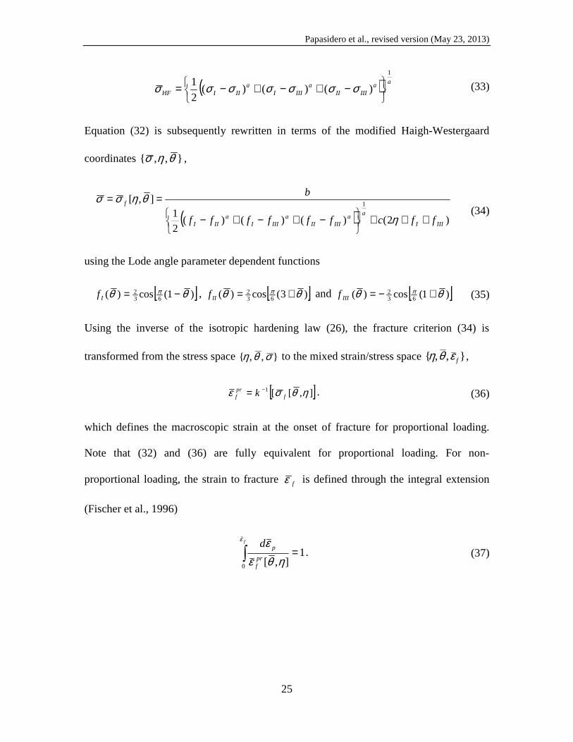
bc IIIIHF =++ )( σσσ (32)

with


25

( ) aaIIIII

aIIII

aIIIHF

1

)()()(2

1

−+−+−= σσσσσσσ (33)

Equation (32) is subsequently rewritten in terms of the modified Haigh-Westergaard

coordinates },,{ θησ ,

( ) )2()()()(2

1],[

1

IIII

aa

IIIIIa

IIIIa

III

f

ffcffffff

b

+++

−+−+−

==

η

θησσ (34)

using the Lode angle parameter dependent functions

[ ])1(cos)( 632 θθ π −=If , [ ])3(cos)( 63

2 θθ π +=IIf and [ ])1(cos)( 632 θθ π +−=IIIf (35)

Using the inverse of the isotropic hardening law (26), the fracture criterion (34) is

transformed from the stress space } , ,{ σθη to the mixed strain/stress space } , ,{ fεθη ,

[ ]],[[1 ηθσε fprf k −= . (36)

which defines the macroscopic strain at the onset of fracture for proportional loading.

Note that (32) and (36) are fully equivalent for proportional loading. For non-

proportional loading, the strain to fracture fε is defined through the integral extension

(Fischer et al., 1996)

∫ =f

prf

pdε

ηθεε

0

1],[

. (37)


26

6.2. Fracture model parameter identification

The HC fracture initiation model features three material parameters: the Hosford

exponent a , the cohesion b , and the friction coefficient c. These parameters are

determined based on the loading paths to fracture for °= 0β (pure shear), °= 55β

(uniaxial tension) and °= 90β (plane strain tension). The identification problem for

},,{ cba corresponds to a non-linear system of three equations

][],,,[ expifi

HCf cba βεβε = for }90,55,0{ °°°=iβ (38)

with HCfε denoting the strain to fracture according to equation (37). After rewriting (38)

as minimization problem, the model parameters 6.1=a , MPab 7.1132= and 053.0=c

are obtained through numerical optimization. The instants at which the calibrated HC

model predicts the onset of fracture are highlighted by blue solid dots in Fig. 12a. These

instants coincide with the ends of the loading paths to fracture for the three calibration

experiments ( °= 0β , °55 and °90 ), whereas the HC model underestimates the strain to

strain to fracture for °= 34β , and overestimates that for °= 69β . The underlying

fracture criterion for proportional loading (Eq. (36)) is depicted in Fig. 12b, showing the

monotonic dependence of the strain to fracture on the stress triaxiality and the

characteristic asymmetric dependence on the Lode angle parameter with a minimum at

0=θ .

We also implemented the HC model into a user material subroutine and repeated the

simulations of all experiments with the fracture initiation criterion being active. The solid

black dots on the curves in Fig. 6 show the instant of fracture as predicted by the HC


27

model. The reasonable agreement with the respective displacements and rotations to

fracture partially confirms the applicability of the HC fracture initiation model and the

validity of the underlying identification procedure. For each loading case, we also

compared the location of the critical element at which fracture initiates according to the

model with that assumed throughout calibration. These locations coincide for °= 0β ,

°5.69 and °90 . However, for °= 34β and °= 55β , the HC model predicts fracture at

slightly different locations as shown by the comparison of the open and solid dots in Fig.

11b. It is thus expected that the model accuracy could be improved further by repeating

the model parameter identification based on the loading paths to fracture extracted from

the predicted locations of onset of fracture.

7. Conclusions

A tubular specimen with a stocky gage section of uniform thickness is proposed to

characterize the effect of stress state on the onset of ductile fracture under tension-torsion

loading. Prior to the onset of necking, the radial gradient in the mechanical fields is small

and plane stress conditions prevail throughout the gage section. At the same time, the

circumferential strain is approximately zero. The theoretical range of achievable stress

triaxialities is -0.58 to 0.58 for a Levy-von Mises material.

Static experiments are performed on specimens extracted from an annealed high

strength steel bar (36NiCrMo16) for positive stress triaxialities. The relative motion of

the specimen shoulders as well as the surface strain fields are determined through stereo

digital image correlation. Finite element simulations are performed of all experiments to


28

estimate the stresses and strains away from the specimen surface. From each experiment,

a loading path to fracture is determined in terms of equivalent plastic strain, stress

triaxiality and Lode angle parameter. It is found that the loading paths obtained from

finite element analysis are substantially different from those determined directly from

surface strain measurements. Except for pure torsion, the equivalent plastic strain reaches

its maximum away from the specimen surface. Furthermore, the stress triaxiality is

significantly higher near the specimen center when fracture initiates after necking. A

hybrid experimental-numerical procedure is outlined and applied to determine the

parameters of the Hosford-Coulomb (HC) fracture initiation model.

Acknowledgement

The financial support of Jessica Papasidero through a Monge Fellowship from Ecole

Polytechnique is gratefully acknowledged. This work was also supported by the Sésame

2006 grants from the Région Ile-de-France. The partial financial support through the

French National Research Agency (Grant ANR-11-BS09-0008, LOTERIE) is gratefully

acknowledged.


29

References

Bai, Y. L. & Wierzbicki, T., 2010, Application of extended Mohr-Coulomb criterion to

ductile fracture, International Journal of Fracture, 161, 1-20

Barsoum I., Faleskog J., 2007, Rupture mechanisms in combined tension and shear –

Experiments, International Journal of Solids and Structures 44, 1768 – 1786

Bornert, M., Bremand, F., Doumalin, P., Dupre, J.-C., Fazzini, M., Grediac, M., Hild, F.,

Mistou, S., Molimard, J., Orteu, J. -J., Robert, L., Surrel, Y., Vacher, P., Wattrisse,

B., 2009. Assessment of Digital Image Correlation Measurement Errors:

Methodology and Results, Experimental Mechanics 49(3), 353-370.

Danas K & Ponte Castañeda P, 2012, Influence of the Lode parameter and the stress

triaxiality on the failure of elasto-plastic porous materials, International Journal of

Solids and Structures 49 (11–12), 1325–1342.

Dunand M, Mohr D, 2013, Effect of Lode Parameter on Plastic Flow Localization at Low

Stress Triaxialities, submitted for publication.

Dunand, M. & Mohr, D., 2010, Hybrid experimental-numerical analysis of basic ductile

fracture experiments for sheet metals, International Journal of Solids and Structures,

47, 1130-1143

Dunand, M. & Mohr, D., 2011, Optimized butterfly specimen for the fracture testing of

sheet materials under combined normal and shear loading, Engineering Fracture

Mechanics, 78, 2919-2934


30

Gao, X. S., Zhang, T. T, Zhou, J., Graham, S. M., Hayden, M., Roe, C., 2011, On stress-

state dependent plasticity modeling: Significance of the hydrostatic stress, the third

invariant of stress deviator and the non-associated flow rule, International Journal of

Plasticity, 27, 217-231

Graham, S. M.; Zhang, T. T.; Gao, X. S.; Hayden, M., 2012, Development of a

combined tension-torsion experiment for calibration of ductile fracture models under

conditions of low triaxiality, International Journal of Mechanical Sciences, 54, 172-

181

Haltom, S.S., Kyriakides, S., Ravi-Chandar, K., “Ductile Failure Under Combined Shear

and Tension.” Int. J. Solids & Structures 40, 1507-1522, 2013

Korkolis, Y. P., Kyriakides, S., Giagmouris, T. , Lee, L. H., 2010, Constitutive Modeling

and Rupture Predictions of Al-6061-T6 Tubes Under Biaxial Loading Paths, Journal

of Applied Mechanics-transactions of the Asme, 77, 064501

Kuwabara, T., Yoshida, K., Narihara, K., Takahashi, S., 2005, Anisotropic plastic

deformation of extruded aluminum alloy tube under axial forces and internal pressure,

International Journal of Plasticity, 21, 101-117

Lindholm, U. S., Nagy, A., Johnson, G. R., Hoegleldt, J. M.,1980, Large Strain, High-

strain Rate Testing of Copper, Journal of Engineering Materials and Technology-

transactions of the Asme,102, 376-381

Mohr, D. & Ebnoether, F., 2009, Plasticity and fracture of martensitic boron steel under

plane stress conditions, Int. J. Solids Struct. 46, 3535–3547


31

Mohr, D. & Henn, S., 2007, Calibration of stress-triaxiality dependent crack formation

criteria: A new hybrid experimental-numerical method, Experimental Mechanics 47,

805-820

Mohr, D. & Marcadet J.M., 2013, Hosford-Coulomb Model for Predicting the Onset of

Ductile Fracture at Low Stress Triaxialities, submitted for publication.

Nahshon K & Hutchinson J. W., 2008, Modification of the Gurson Model for shear

failure, European Journal of Mechanics A/Solids 27, 1 – 17

Nielsen, K. L. & Tvergaard, V., 2011, Failure by void coalescence in metallic materials

containing primary and secondary voids subject to intense shearing, International

Journal of Solids and Structures, 48, 1255-1267

Nouailhas, D., Cailletaud, G., 1995, Tension-torsion Behavior of Single-crystal

Superalloys - Experiment and Finite-element Analysis, International Journal of

Plasticity, 11, 451-470

Sung JH, Kim JH, Wagoner RH, 2010, A plastic constitutive equation incorporating

strain, strain-rate, and temperature, International Journal of Plasticity 26, 1746-1771.

Sutton MA, Orteu JJ, Schreier H, 2009, Image Correlation for Shape, Motion and

Deformation Measurements: Basic Concepts, Theory and Applications, Springer.

Teng, X., Mae, H., Bai, Y., Wierzbicki, T., 2009, Pore size and fracture ductility of

aluminum low pressure die casting, Engineering Fracture Mechanics, 76, 983-996

Zhang, J. X. & Jiang, Y. Y., 2005, Luders bands propagation of 1045 steel under

multiaxial stress state, International Journal of Plasticity, 21, 651-670


32

Tables Table 1. Chemical composition of 36NiCrMo16 provided by ThyssenKrupp Steel (in weight %)

C Mn Si S P Cr Ni

Mo

Cu

Al

0.37 0.41 0.25 0.016 0.011 1.72 3.74 0.28 0.25 0.03

Table 2. Loading conditions.

°= 0β °= 1.34β °= 55β °= 5.69β °= 90β

0.02 °/s 0kN

0.01°/s F=0.0645M

0.005°/s F=0.135M

4.10-4mm/s M=3.9F

0.0012mm/s 0N.m

Table 3. Hardening parameters

A εo n ko Q b

[MPa] [−] [−] [MPa] [MPa] [−]

Seed 529.4 3.10-3 0.08 372.3 146.4 4.64

Final 712 7.10-5 0.13 307 92 3.24


33

Figures

(a) (b)

Figure 1. (a) Schematic of specimen geometry, (b) geometry parameters and FE mesh.

M

F


34

(a)

(b)

Figure 2. Stress distribution inside the gage section prior to necking: (a) Influence of the

gage section height h on stress state uniformity along the radial direction (b) variation of

the radial stress along the radial direction. A radial coordinate of 0 and 1 corresponds to

the inner and outer gage section surface, respectively. Note that the free surface condition

0=rrσ appears to be only approximately fulfilled due to the normalized ordinate axis.

Radial coordinate [-]

torsion

tension

Radial coordinate [-]

Ra

dia

l st

ress

[-

]

tension-

torsion


35

Figure 3. Theoretical range of stress states achievable with the current geometry.

Stress triaxiality [-]

Lod

e a

ng

le p

ara

me

ter

[-]

uniaxial

tension

Plane strain

tension

pure

shear


36

Figure 4. Optical micrograph after 20s of swab etching with Villela’s reagent


37

(a)

(b) (c)

Figure 5. (a) Photograph of the experimental setup showing 1-specimen, 2-axial/torsion

load cell, 3-piston, 4-cameras, 5-lighting, (b) left camera view of the specimen with DIC

area of interest (AOI) highlighted, (c) specimen dimensions.

1

2

4 4

5 5

3

AOI

5mm

A

B


38

(a)

(b)

Figure 6. (a) Axial force-displacement and (b) torque-rotation curves for different biaxial

loading angles. The solid black dots on the dashed simulation curves indicate the instant

of onset of fracture as predicted by the Hosford-Coulomb model.

β=90°

β=55°

β=34.1°

β=69.5°

β=34.1°

β=55°

β=69.5°

β=0°


39

(a)

(b)

(c)

Figure 7. Loading paths: (a) nominal shear versus axial strain, (b) nominal

circumferential versus axial strain, (c) average true shear versus true normal stress, (d)

evolution of the Lode angle parameter and the stress triaxiality as predicted by FEA.

β=90°

β=55°β=34.1°

β=69.5°

β=0°

β=90°

β=55°

β=34.1°β=69.5°

εθ=-0.1εz

β=90°

β=55°β=34.1°β=0°`

β=69.5°

(a)

(c)

(e)

Figure 8. Photographs of the f

onset of fracture. (a)-(b) =β

Papasidero et al., revised version (

40

(b)

(d)

(f)

Photographs of the fractured specimens and measured surface strain fields at the

°= 90 , (c)-(d) °= 55β , (e)-(f) °= 0β .

ed version (May 23, 2013)

and measured surface strain fields at the


41

(a) (b) (c)

(d) (e) (f)

(g) (h) (i)

Figure 9. Evolution of the surface strains throughout loading: (a)-(c) °= 90β , (d)-(f)

°= 55β , and (g)-(i) °= 0β . The solid (dashed) lines in the central plots correspond to

the strains obtained from the displacement measurements with (without) averaging over a

mµ200 period. The rightmost column shows longitudinal cuts through the fractured

specimens.

1 2 34

1

2

3

4

[-]

500 µµµµm

1 2 3

4

[-]

1

2

3

4

500 µµµµm

1 2 3 4

1

2

3

4

[-]

500 µµµµm


42

Figure 10. Identification of the isotropic hardening law.

optimized

Swift (seed)

experimental

Voce (seed)


43

(a)

(b)

Figure 11. (a) Loading paths to fracture as determined using the (i) Surface-strain based

method (dashed red lines), and (ii) full FEA method; (b) distribution of the equivalent

plastic strain within the specimen cross-section at the onset of fracture as obtained from

FEA. The solid dots indicate the locations of loading path extraction. For °= 1.34β and

°55 , an open dot highlights the location of onset of fracture as predicted by the Hosford-

Coulomb model.

Stress triaxiality

Eq

uiv

. p

last

ic s

tra

in

0o

34.1o 55

o

69.5o

90o

z=0

β=90°β=55°β=34.1° β=69.5°β=0°


44

(a)

(b)

Figure 12. (a) Predictions of the onset of fracture according to the calibrated Hosford-

Coulomb model (blue dots), (b) 3D plot of the fracture initiation model for proportional

loading.

fε

θη

determination of the effect of stress state on the onset

Documents