determination of optimum classification · pdf filedetermination of optimum classification...
TRANSCRIPT
DETERMINATION OF OPTIMUM CLASSIFICATION SYSTEM FOR
HYPERSPECTRAL IMAGERY AND LIDAR DATA BASED ON BEES ALGORITHM
F. Samadzadegan a, H. Hasani a, *
a School of Surveying and Geospatial Engineering, College of Engineering, University of Tehran, Tehran, Iran –
(samadz, hasani)@ut.ac.ir
Commission I, ICWG III/VII
KEY WORDS: Hyperspectral, LiDAR, Fusion, SVM Classifier, Optimization, Parameter Determination, Feature Selection, Bees
Algorithm
ABSTRACT:
Hyperspectral imagery is a rich source of spectral information and plays very important role in discrimination of similar land-cover
classes. In the past, several efforts have been investigated for improvement of hyperspectral imagery classification. Recently the interest
in the joint use of LiDAR data and hyperspectral imagery has been remarkably increased. Because LiDAR can provide structural
information of scene while hyperspectral imagery provide spectral and spatial information. The complementary information of LiDAR
and hyperspectral data may greatly improve the classification performance especially in the complex urban area. In this paper feature
level fusion of hyperspectral and LiDAR data is proposed where spectral and structural features are extract from both dataset, then
hybrid feature space is generated by feature stacking. Support Vector Machine (SVM) classifier is applied on hybrid feature space to
classify the urban area. In order to optimize the classification performance, two issues should be considered: SVM parameters values
determination and feature subset selection. Bees Algorithm (BA) is powerful meta-heuristic optimization algorithm which is applied
to determine the optimum SVM parameters and select the optimum feature subset simultaneously. The obtained results show the
proposed method can improve the classification accuracy in addition to reducing significantly the dimension of feature space.
1. INTRODUCTION
Recently, with the progress in remote sensing technologies, it is
possible to measure different characteristics of objects on the
earth such as spectral, height, amplitude and phase information
by multispectral/hyperspectral, LiDAR and SAR respectively
(Debes et al. 2014). Availability of different types of data,
provides means of detecting and discriminating of land use land
cover in complex urban area (Ramdani, 2013). Classification of
urban area has been used in wide range of application, such as
mapping and tracking, risk management, social and ecological
problems (Fauvel, 2007).
Hyperspectral remote sensing data is characterized by a very high
spectral resolution that usually results in hundreds of observation
bands. According to spectral richness, it plays very important
role in discrimination of land-cover with similar spectral
reflectance (Chang, 2013). Although hyperspectral imagery
provides comprehensive spectral information but classification
of complex urban area based on just spectral information has
some limitations: same objects with different spectral
characteristic don’t classify in a class (e.g. buildings with
different roof material/color don’t classify in one class) and
different objects with same spectral appearance may classify in
same class (e.g. tree and grass/ roof and road). On the other hand,
LiDAR sensor provides 3D information from surfaces and
mapping with LiDAR data depend on the ability to detect objects
with different height. There is a complementary relationship
between passive hyperspectral images and active LiDAR data, as
they contain very different information (Khodadazadeh et al.
2015).
* Corresponding author
According to availability, robustness and accuracy of spectral
and structural information of hyperspectral images and LiDAR
data, fusion of hyperspectral images and LiDAR data in a joint
classification system, may yield more reliable and accurate
classification results. While there have been numerous
investigations that have reported on the use of other multisensory
data (e.g. LiDAR and Multispectral), very few results are
available about simultaneously integration of these two data
sources in classification tasks (Debes et al. 2014, Latifi et al.
2012).
This paper presents an optimum hybrid classification system by
simultaneous determination of the SVM parameters and the
selection of features through swarm optimization process in order
to fuse hyperspectral imagery and LiDAR data.
2. RELATED WORK
During last years, some investigations were carried out on
fusion/integration of hyperspectral images and LiDAR data in
different application, such as forest structure analysis, urban area
mapping, identification of tree species, forest fire management,
etc. (Alonzo et al. 2014, Brook et al., 2010, Dalponte et al. 2008,
Koetz et al. 2008, Latifi et al. 2012). In some research works,
LiDAR data is used for separation of 2D and 3D objects and then
hyperspectral images are applied to discriminate among different
species of an object, such as roofing material (Niemann, et al.,
2009; Zhang and Qiu, 2012). Sugumaran and Voss (2007), apply
the object based classification where LiDAR data is used for
segmentation and hyperspectral image to classify the segments.
Dalponte et al. (2008) merge a subset of hyperspectral bands with
two LiDAR imaging data (intensity and nDSM), then fuse it with
The International Archives of the Photogrammetry, Remote Sensing and Spatial Information Sciences, Volume XL-1/W5, 2015 International Conference on Sensors & Models in Remote Sensing & Photogrammetry, 23–25 Nov 2015, Kish Island, Iran
This contribution has been peer-reviewed. doi:10.5194/isprsarchives-XL-1-W5-651-2015
651
results of the image classified by SVM and Gaussian Mixture
Model. Liu et al. (2011) compute Canopy Height Model (CHM)
from first LiDAR return and Minimum Noise Fraction (MNF)
transformation is executed based on the pixel-level fusion of
hyperspectral imagery and CHM channels. Then the first 26
eigenvalue bands are kept as input data for SVM classifier. Latifi
et al. (2012) fuse hyperspectral bands and LiDAR features using
Genetic Algorithm (GA) and apply this to select the feature
subset in order to model forest structure.
In order to optimize the classification performance of high
dimensional data, several methods are proposed in literatures
which can be categorized into three groups: parameter
determination of classifier (Liu et al. 2014), feature selection
(Rashedi and Nezamabadi-pour, 2014) and simultaneously
consider both of them (Samadzadegan, et al. 2012). The
parameters of classifier has significant effect on its performance
where grid search is common way to determine them (Hsu et al.
2003). Moreover, the selection of the feature subset may affect
several classification aspects, including classification accuracy,
computation time, training sample size, and the cost associated
with the features (Lin et al., 2008). Several studies are focused
on optimization these two issues which show that according to
the dependency of parameters and features, simultaneous
parameter determination and feature selection yield the most
accurate results (O'Boyle et al., 2008). Recently Liu et al. applied
PSO to determine the SVM kernel and margin parameters in
classification of hyperspectral imagery and the results compared
with grid search method which show the superiority of the
proposed method (Liu et al. 2014). Feature selection is another
essential step in classification of high dimension data. Rashedi
and Nezamabadi-pour (2014) proposed an improved version of
the binary gravitational search algorithm as a tool to select the
best subset of features with the goal of improving classification
accuracy. As parameter values effect on feature subset selection
and vice versa, Samadzadegan et al. (2012) show that the best
performance of classification is obtained by simultaneously
classifier determination and feature selection by Ant Colony
Optimization.
In this paper an optimum hybrid classification system is
presented that simultaneously determines SVM classifier
parameters and selects the feature subset to optimize
classification performance for combined hyperspectral imagery
and LiDAR data.
3. PROPOSED METHOD
In order to fuse hyperspectral imagery and LiDAR data, a hybrid
feature space consisting of spectral and structural features is
generated. Spectral feature space composed of original
hyperspectral bands, vegetation indices and principle
components. On the other hand, textural analysis on normalized
DSM (nDSM), roughness and its textures, slope descriptors are
extracted from LiDAR data which make the structural feature
space. By combining spectral and structural feature space, the
hybrid feature space is defined. Then normalization is used to
transform data into the range [0, 1], in order to reduce numerical
complexity.
According to the stability of SVM in high dimensional space [5],
SVM is selected as classifier. There are two important challenges
in classification of high dimensional data by a SVM classifier:
SVM parameter determination (kernel and regularization
parameters) and feature subset selection. In order to optimize
classification of this hybrid feature space based on SVM,
optimized SVM parameters values and appropriate feature
subsets should be selected. For this purpose the Binary Bees
Algorithm, as a powerful population based optimization
algorithm, is applied to determine SVM parameters and selection
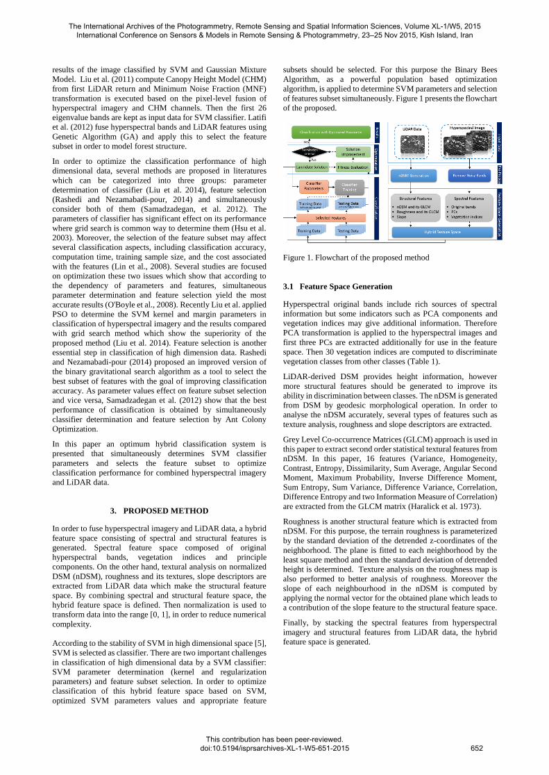
of features subset simultaneously. Figure 1 presents the flowchart
of the proposed.
Figure 1. Flowchart of the proposed method
3.1 Feature Space Generation
Hyperspectral original bands include rich sources of spectral
information but some indicators such as PCA components and
vegetation indices may give additional information. Therefore
PCA transformation is applied to the hyperspectral images and
first three PCs are extracted additionally for use in the feature
space. Then 30 vegetation indices are computed to discriminate
vegetation classes from other classes (Table 1).
LiDAR-derived DSM provides height information, however
more structural features should be generated to improve its
ability in discrimination between classes. The nDSM is generated
from DSM by geodesic morphological operation. In order to
analyse the nDSM accurately, several types of features such as
texture analysis, roughness and slope descriptors are extracted.
Grey Level Co-occurrence Matrices (GLCM) approach is used in
this paper to extract second order statistical textural features from
nDSM. In this paper, 16 features (Variance, Homogeneity,
Contrast, Entropy, Dissimilarity, Sum Average, Angular Second
Moment, Maximum Probability, Inverse Difference Moment,
Sum Entropy, Sum Variance, Difference Variance, Correlation,
Difference Entropy and two Information Measure of Correlation)
are extracted from the GLCM matrix (Haralick et al. 1973).
Roughness is another structural feature which is extracted from
nDSM. For this purpose, the terrain roughness is parameterized
by the standard deviation of the detrended z-coordinates of the
neighborhood. The plane is fitted to each neighborhood by the
least square method and then the standard deviation of detrended
height is determined. Texture analysis on the roughness map is
also performed to better analysis of roughness. Moreover the
slope of each neighbourhood in the nDSM is computed by
applying the normal vector for the obtained plane which leads to
a contribution of the slope feature to the structural feature space.
Finally, by stacking the spectral features from hyperspectral
imagery and structural features from LiDAR data, the hybrid
feature space is generated.
The International Archives of the Photogrammetry, Remote Sensing and Spatial Information Sciences, Volume XL-1/W5, 2015 International Conference on Sensors & Models in Remote Sensing & Photogrammetry, 23–25 Nov 2015, Kish Island, Iran
This contribution has been peer-reviewed. doi:10.5194/isprsarchives-XL-1-W5-651-2015
652
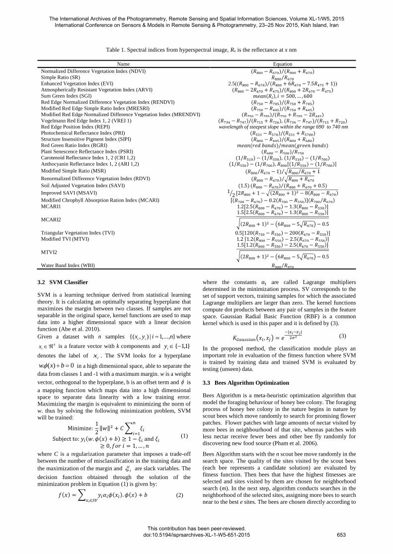
Table 1. Spectral indices from hyperspectral image, Rx is the reflectance at x nm
Name Equation
Normalized Difference Vegetation Index (NDVI) (𝑅800 − 𝑅670) (𝑅800 + 𝑅670)⁄ Simple Ratio (SR) 𝑅800 𝑅670⁄ Enhanced Vegetation Index (EVI) 2.5((𝑅800 − 𝑅670) (𝑅800 + 6𝑅670 − 7.5𝑅475 + 1)⁄ )
Atmospherically Resistant Vegetation Index (ARVI) (𝑅800 − 2𝑅670 + 𝑅475)/(𝑅800 + 2𝑅670 − 𝑅475) Sum Green Index (SGI) 𝑚𝑒𝑎𝑛(𝑅𝑖), 𝑖 = 500, … , 600 Red Edge Normalized Difference Vegetation Index (RENDVI) (𝑅750 − 𝑅705)/(𝑅750 + 𝑅705) Modified Red Edge Simple Ratio Index (MRESRI) (𝑅750 − 𝑅445)/(𝑅750 + 𝑅445) Modified Red Edge Normalized Difference Vegetation Index (MRENDVI) (𝑅750 − 𝑅705)/(𝑅750 + 𝑅705 − 2𝑅445) Vogelmann Red Edge Index 1, 2 (VREI 1) (𝑅734 − 𝑅747)/(𝑅715 + 𝑅726), (𝑅734 − 𝑅747)/(𝑅715 + 𝑅720) Red Edge Position Index (REPI) wavelength of steepest slope within the range 690 to 740 nm
Photochemical Reflectance Index (PRI) (𝑅531 − 𝑅570)/(𝑅531 + 𝑅5700) Structure Insensitive Pigment Index (SIPI) (𝑅800 − 𝑅445)/(𝑅800 + 𝑅680) Red Green Ratio Index (RGRI) 𝑚𝑒𝑎𝑛(𝑟𝑒𝑑 𝑏𝑎𝑛𝑑𝑠)/𝑚𝑒𝑎𝑛(𝑔𝑟𝑒𝑒𝑛 𝑏𝑎𝑛𝑑𝑠)
Plant Senescence Reflectance Index (PSRI) (𝑅680 − 𝑅500)/𝑅750 Carotenoid Reflectance Index 1, 2 (CRI 1,2) (1/𝑅510) − (1/𝑅550), (1/𝑅510) − (1/𝑅700)
Anthocyanin Reflectance Index 1, 2 (ARI 1,2) (1/𝑅550) − (1/𝑅700), 𝑅800[(1/𝑅550) − (1/𝑅700)]
Modified Simple Ratio (MSR) (𝑅800 𝑅670⁄ − 1) √𝑅800 𝑅670⁄ + 1⁄
Renormalized Difference Vegetation Index (RDVI) (𝑅800 − 𝑅670) √𝑅800 + 𝑅670⁄
Soil Adjusted Vegetation Index (SAVI) (1.5) (𝑅800 − 𝑅670) (𝑅800 + 𝑅670 + 0.5)⁄
Improved SAVI (MSAVI) 12⁄ [2𝑅800 + 1 − √(2𝑅800 + 1)2 − 8(𝑅800 − 𝑅670)
Modified Chrophyll Absorption Ration Index (MCARI) [(𝑅700 − 𝑅670) − 0.2(𝑅700 − 𝑅550)](𝑅700 𝑅670⁄ ) MCARI1 1.2[2.5(𝑅800 − 𝑅670) − 1.3(𝑅800 − 𝑅550)]
MCARI2
1.5[2.5(𝑅800 − 𝑅670) − 1.3(𝑅800 − 𝑅550)]
√(2𝑅800 + 1)2 − (6𝑅800 − 5√𝑅670) − 0.5
Triangular Vegetation Index (TVI) 0.5[120(𝑅750 − 𝑅550) − 200(𝑅670 − 𝑅550)] Modified TVI (MTVI) 1.2 [1.2(𝑅800 − 𝑅550) − 2.5(𝑅670 − 𝑅550)]
MTVI2
1.5[1.2(𝑅800 − 𝑅550) − 2.5(𝑅670 − 𝑅550)]
√(2𝑅800 + 1)2 − (6𝑅800 − 5√𝑅670) − 0.5
Water Band Index (WBI) 𝑅900 𝑅970⁄
3.2 SVM Classifier
SVM is a learning technique derived from statistical learning
theory. It is calculating an optimally separating hyperplane that
maximizes the margin between two classes. If samples are not
separable in the original space, kernel functions are used to map
data into a higher dimensional space with a linear decision
function (Abe et al. 2010).
Given a dataset with n samples },...,1|),{( niyx ii where
k
ix is a feature vector with k components and }1,1{iy
denotes the label of ix . The SVM looks for a hyperplane
0)(. bxw in a high dimensional space, able to separate the
data from classes 1 and -1 with a maximum margin. w is a weight
vector, orthogonal to the hyperplane, b is an offset term and is
a mapping function which maps data into a high dimensional
space to separate data linearity with a low training error.
Maximizing the margin is equivalent to minimizing the norm of
w. thus by solving the following minimization problem, SVM
will be trained:
Minimize: 1
2‖𝑤‖2 + 𝐶 ∑ 𝜉𝑖
𝑛
𝑖=1
Subject to: 𝑦𝑖(𝑤. 𝜙(𝑥) + 𝑏) ≥ 1 − 𝜉𝑖 and 𝜉𝑖
≥ 0, 𝑓𝑜𝑟 𝑖 = 1, … , 𝑛
(1)
where C is a regularization parameter that imposes a trade-off
between the number of misclassification in the training data and
the maximization of the margin and i are slack variables. The
decision function obtained through the solution of the
minimization problem in Equation (1) is given by:
𝑓(𝑥) = ∑ 𝑦𝑖𝛼𝑖𝜙(𝑥𝑖). 𝜙(𝑥) + 𝑏𝑥𝑖∈𝑆𝑉
(2)
where the constants αi are called Lagrange multipliers
determined in the minimization process. SV corresponds to the
set of support vectors, training samples for which the associated
Lagrange multipliers are larger than zero. The kernel functions
compute dot products between any pair of samples in the feature
space. Gaussian Radial Basic Function (RBF) is a common
kernel which is used in this paper and it is defined by (3).
𝐾𝐺𝑎𝑢𝑠𝑠𝑖𝑎𝑛(𝑥𝑖 , 𝑥𝑗) = 𝑒−|𝑥𝑖−𝑥𝑗|
2𝜎2 (3)
In the proposed method, the classification module plays an
important role in evaluation of the fitness function where SVM
is trained by training data and trained SVM is evaluated by
testing (unseen) data.
3.3 Bees Algorithm Optimization
Bees Algorithm is a meta-heuristic optimization algorithm that
model the foraging behaviour of honey bee colony. The foraging
process of honey bee colony in the nature begins in nature by
scout bees which move randomly to search for promising flower
patches. Flower patches with large amounts of nectar visited by
more bees in neighbourhood of that site, whereas patches with
less nectar receive fewer bees and other bee fly randomly for
discovering new food source (Pham et al. 2006).
Bees Algorithm starts with the n scout bee move randomly in the
search space. The quality of the sites visited by the scout bees
(each bee represents a candidate solution) are evaluated by
fitness function. Then bees that have the highest fitnesses are
selected and sites visited by them are chosen for neighborhood
search (m). In the next step, algorithm conducts searches in the
neighborhood of the selected sites, assigning more bees to search
near to the best e sites. The bees are chosen directly according to
The International Archives of the Photogrammetry, Remote Sensing and Spatial Information Sciences, Volume XL-1/W5, 2015 International Conference on Sensors & Models in Remote Sensing & Photogrammetry, 23–25 Nov 2015, Kish Island, Iran
This contribution has been peer-reviewed. doi:10.5194/isprsarchives-XL-1-W5-651-2015
653

the fitnesses associated with the sites they are visiting. Searches
in the neighborhood of the best e sites which represent more
promising solutions are made more detailed by recruiting more
bees to follow them than the other selected bees (m-e). Together
with scouting, this differential recruitment is a key operation of
the Bees Algorithm.
However for each patch only the bee with the highest fitness will
be selected to for the next bee population. In nature, there is no
such a restriction. This restriction is introduced here to reduce the
number of points to be explored. Then, the remaining bees in the
population are assigned randomly around the search space
scouting for new potential solutions. These steps are repeated
until a stopping criterion is met (Pham et al. 2006).
3.4 Determination of Optimum Classification System for
Classification of Hyperspectral Imagery and LiDAR Based
on Bees Algorithm
In order to determine the SVM parameters values and feature
subset simultaneously based on Bees Algorithm, binary coding
is applied. In the proposed method, binary string composed of
three main parts is considered: features, regularization parameter
and kernel parameter. The first part of binary string consist of nf
bits equal to dimension of feature space. Where '0' and ‘1’ in the
ith bit means that ith feature should be discard and considered,
respectively. Regularization and kernel parameters are real-
valued and transform to binary coding for consistency with the
binary nature of the feature selection process. The length of
regularization (nc) and kernel parameters (nk) depends on the
range of the parameters and the required precision.
Evaluation of the candidate solution is done by using a fitness
function. The first part of the binary of the solution define which
feature should be selected. For the determination of the SVM
parameters, the binary format of the second and third parts of the
solution converts to a real-value, expressed by Equation (4).
𝑝 = 𝑚𝑖𝑛𝑝 +𝑚𝑎𝑥𝑝 − 𝑚𝑖𝑛𝑝
2𝑙 − 1× 𝑑 (4)
where p is the real value of the bit string, minp and maxp are
minimum and maximum values of the parameter p, determined
by the user. l is the length of the bit string (for each parameter)
and d is a decimal value of the bit string.
Results may have fewer selected features and a higher
classification accuracy. The combination of classification
accuracy and the number of selected features constitutes the
evaluation function. Multiple criteria problems can be solved by
creating a single objective fitness function that combines the two
goals into one. The objective function is defined by Equation (5).
𝑓 = 𝜌 × (1 − 𝑎𝑐𝑐𝑢𝑟𝑎𝑐𝑦) + (1 − 𝜌) ×1
𝑁𝑓
(5)
where f is the fitness value, 𝜌 is a constant parameter in [0,1],
accuracy obtained by Kappa coefficient and Nf is the number of
selected features.
The proposed method starts with generation of the candidate
solutions which are formed randomly at the first iteration. Then
each bee (represent by candidate solution) is evaluated by
Equation (5) and the bee with higher classification accuracy and
the lowest selected feature subset is selected as promising
solution for the population (with maximum fitness value).
Neighbourhood search around the best solutions is performed by
changing the value of a random bit of that solutions. Other bees
are search randomly by generating the random binary string
which show the candidate solutions. This process is iterated till
the termination criterion (maximum iteration) is satisfied.
4. EXPERIMENTAL RESULTS
To evaluate the performance of the proposed method,
experiments are performed on Compact Airborne Spectrographic
Imager (CASI) hyperspectral imagery and LiDAR derived DSM
acquired by the NSF-funded Center for Airborne Laser Mapping
(NCALM), both at the same spatial resolution (2.5 m). The
hyperspectral imagery consists of 144 spectral bands in the
spectral range between 380 nm to 1050 nm and the corresponding
co-registered DSM consists of elevation in meters above sea
level (Geoid 2012A model).
Figure 2. (a) LiDAR derived DSM (b) Hyperspectral imagery
Land cover classes consist of three types of grass (healthy,
stressed and synthetic), road, soil, residential and commercial
buildings. Spectral features (144 spectral bands, 30 vegetation
indices and 3 PCs) have ability to discriminate different grass
types and 2D objects; however referring to similar geometrical
structure and height, LiDAR data cannot provide more
information. On the other hand, spectral similarity of tree and
grass/ roof and road may cause hyperspectral encounter some
challenges but according to the height difference, fusion of
hyperspectral imagery and LiDAR data may improve
discrimination of complex urban objects.
4.1 Feature Space Generation
Generation of feature space is performed by processing both
hyperspectral imagery and LiDAR data. Hyperspectral image
was acquired by the CASI sensor and it has 144 bands. Moreover
30 vegetation indices are computed (Table 1). PCA
transformation is applied on hyperspectral imagery and 3 first
PCs with more than 99% eigenvalues are selected to complete
spectral feature space. Consequently, the spectral feature space
compose of 177 descriptors.
DSM derived from LiDAR data is a source of structural
information. Geodesic morphological operation with circular
structural element is applied on the DSM to create nDSM.
Texture analysis of nDSM is performed based on GLCM features
that 16 descriptors are extracted. Then roughness map and its 16
textural descriptors are also computed. Slope is further descriptor
which is useful in classification, extracted from nDSM.
Therefore the structural feature space is generated by merging all
these 35 features.
By merging, spectral and structural feature space, a hybrid image
is generated that contains rich information content for each pixel
and forms our feature space with 212 features for pixel-based
classification.
4.2 Classification Based on SVM
SVM classifier is applied to evaluate the quality of hybrid feature
space. The SVM classification was done by using the LIBSVM
through its Matlab interface (Chang and Lin, 2001). The Kappa
coefficient and the overall accuracy are commonly used to
determine the classification accuracy. These criteria were used to
(a) (b)
The International Archives of the Photogrammetry, Remote Sensing and Spatial Information Sciences, Volume XL-1/W5, 2015 International Conference on Sensors & Models in Remote Sensing & Photogrammetry, 23–25 Nov 2015, Kish Island, Iran
This contribution has been peer-reviewed. doi:10.5194/isprsarchives-XL-1-W5-651-2015
654

compare classification results and were computed by using the
confusion matrix.
Ground truth samples are divided into training and testing data
sets. The SVM classifier is trained based on training data and the
best parameters are tuned and the classification performance is
evaluated by unseen data (testing data). Among 7 classes, the
classes tree, residential and commercial are placed in the “3D
objects group”, where fusion of LiDAR and hyperspectral data
may improve classification results. For 2D objects, hyperspectral
data are an efficient tool for discrimination among them.
However 2D objects are commonly grouped as ground level in
LiDAR data but the data are also useful in separating 2D and 3D
objects.
Table 2 present the results of SVM classification along with
determined parameters (based on grid search) for hyperspectral,
LiDAR, spectral, spatial and hybrid feature space.
Table 2. Classification accuracy and SVM parameters
Dataset C Gamma Kappa OA
Hyperspectral 128 1 0.82 84.78%
LiDAR 1028 8 0.29 33.65%
Spectral 64 0.25 0.84 86.74%
Structural 64 0.25 0.47 52.35%
Hybrid Feature 4 0.25 0.87 89.13%
Obtained results show that LiDAR data are not accurate enough
to classify the dataset, however by extracting the structural
features, the classification accuracy improves significantly. On
the other side hyperspectral data show comparable results with
respect to the hybrid feature space. However the hybrid image
still exhibits a superior performance through the fusion of two
datasets with different information content.
4.3 Results of the Proposed Method
Although the hybrid image improve the classification accuracy,
but there are several correlated and redundant features which
degrade classification performance. On the other side the SVM
parameters is another important elements in classification. SVM
parameters influence on feature subset selection and vice versa,
therefore in this section simultaneous SVM parameters tuning
and feature subset selection based on Bees Algorithm is
performed. Table 3 contains important values for the Bees
Algorithm.
Table 3. Parameters values of Bees Algorithm
Parameters Values
Number of bee (n) 30
Number of best bees (m) 15
Number of elite (e) 5
Neighbourhood (Ne) 4
Neighbourhood best (Nm-e) 2
Iteration (t) 100
Figure 3 shows the convergence plots for the Bees Algorithm
procedures in spectral and structural features and hybrid feature
space. The fitness value for the best individual in each generation
is shown. The weight parameter in objective function (Equation
5) is set to 𝜌 = 0.8 which considers 80% of fitness to accuracy
and 20% to dimensionality of feature space.
Figure 3. Convergence plot of the fitness value
Table 4 contains the number of selected features, as well as the
values of regularization and kernel parameters and the
classification accuracy for testing dataset, determined with the
proposed method for spectral and structural and hybrid feature
space.
Table 4. Results of the proposed method
Dataset # Feature C Gamma Kappa OA
Spectral 81 131.5 0.175 0.87 89.65%
Structural 20 57.3 0.265 0.51 53.89%
Hybrid 101 76.34 0.274 0.901 92.53%
Analysing Table 4 reveals that applying the proposed method on
hybrid image yields the best performance with respect to each
dataset separately.
Comparing the results of hyperspectral imagery classification
with the optimized classification system of hybrid images show
that using DSM beside hyperspectral imagery and optimization
of the SVM parameter and selection of feature subset, improve
classification system approximately 8%, moreover it eliminate
111 redundant features.
5. CONCLUSION
This study investigates the framework for optimization of a
hybrid classification system to fuse hyperspectral and LiDAR
data based on Bees Algorithm. Experiments were carried out
using CASI hyperspectral image data and a DSM derived from
LiDAR data. Several spectral and structural features were
extracted from hyperspectral and LiDAR data respectively.
Although SVM is an appropriate classifier for this high
dimensional space, its performance is optimized by
simultaneously determination of parameters and selection of
feature subsets.
The obtained results show that utilizing 3D information from
LiDAR data in addition to high spectral information of
hyperspectral data, improves the classification performance.
Optimization of the hybrid classification system based on Bees
Algorithm improves classification accuracy about 3.5% along
with the elimination of 111 redundant features. Therefore the
optimum hybrid classification system reaches more accurate
results in a less complex space.
ACKNOWLEDGEMENTS
The authors would like to thank the Hyperspectral Image
Analysis group and the NSF Funded Center for Airborne Laser
0.34
0.39
0.44
0.49
0.54
0.59
0.64
0.69
0.74
1 10 19 28 37 46 55 64 73 82 91 100
Spectral Structural Hybrid
The International Archives of the Photogrammetry, Remote Sensing and Spatial Information Sciences, Volume XL-1/W5, 2015 International Conference on Sensors & Models in Remote Sensing & Photogrammetry, 23–25 Nov 2015, Kish Island, Iran
This contribution has been peer-reviewed. doi:10.5194/isprsarchives-XL-1-W5-651-2015
655
Mapping (NCALM) at the University of Houston for providing
the data sets used in this study, and the IEEE GRSS Data Fusion
Technical Committee for organizing the 2013 Data Fusion
Contest.
REFERENCES
Alonzo, M., Bookhagen, B., Roberts, D.A., 2014. Urban tree
species mapping using hyperspectral and lidar data fusion.
Remote Sensing of Environment, Vol. 148, pp. 70-83.
Brook, A., Ben-Dor, E., Richter, R., 2010. Fusion of
Hyperspectra Images and LiDAR Data for Civil Engineering
Structure Monitoring. 2nd workshop on hyperspectral image and
signal processing: Evolution in Remote Sensing (WHISPERS),
pp. 1-5.
Chang, C. I. Hyperspectral Data Processing: Algorithm Design
and Analysis, JohnWiley & Sons, Inc., USA, 2013.
Dalponte, M., Bruzzone, L., and Gianelle, D., 2008. Fusion of
Hyperspectral and LIDAR Remote Sensing Data for
Classification of Complex Forest Area. IEEE Transaction on
Geoscience and Remote Sensing, Vol. 46, No. 5, pp. 1416-1427.
Debes, C., Merentitis, A., Heremans, R., Hahn, J., Frangiadakis,
N., van Kasteren, T., Liao, W., Bellens, R., Pizurica, A.,
Gautama, S. and Philips, W., Prasad, S., Du, Q., Pacifici, F.,
2014. Hyperspectral and LiDAR data fusion: Outcome of the
2013 GRSS Data Fusion Contest. IEEE Journal of Selected
Topics in Applied Earth Observations and Remote Sensing.
Fauvel, M., (2007). Spectral and Spatial Method for
Classification of Urban Remote Sensing Data, Ph.D thesis.
Haralick, R.M., Shanmugam, K., Dinstein, I., 1973. Textural
Features for Image Classification. IEEE Transaction on Systems,
Man and Cybernetics, Vol. SMC-3, No. 6, pp. 610-621.
Hsu, C.W., Chang, C.C., and Lin, C.J., 2003. A Practical Guide
to Support Vector Classification, National Technical Report,
Taiwan University.
Khodadadzadeh, M., Li, J., Prasad, S., Plaza, A., (2015). Fusion
of Hyperspectral and LiDAR Remote Sensing Data Using
Multiple Feature Learning. IEEE Journal of Selected Topics in
Applied Earth Observations and Remote Sensing, Vol. 8, No. 6.
Koetz, B., Morsdorf, F., van der Linden, S., Curt, T., Allgöwer,
B., 2008. Multi-source Land Cover Classification for Forest Fire
Management based on Imaging Spectrometry and LiDAR data.
Forest Ecology and Management, Vol. 256, pp. 263-271.
Latifi, H., Fassnacht, F., Koch, B., 2012. Forest Structure
Modeling with Combined Airborne Hyperspectral and LiDAR
Data. Remote sensing of Environment, Vol. 121, pp.10-25.
Lin, S.W., Ying, K.C., Chen, S.C., and Lee, Z.J., 2008. Particle
Swarm Optimization for Parameter Determination and Feature
Selection of Support Vector Machines. Expert Systems with
Applications, Vol. 35, No. 4, pp. 1817-1824.
Liu, Q.J., Jing, L.H., Wang, L.M., Lin, Q.Z., 2014. A Method of
Particle Swarm Optimized SVM Hype-spectral Remote Sensing
Image Classification. 35th International Symposium on Remote
Sensing of Environment.
Niemann, O.O., Gordon, W.F., Rafael, L., Fabio, V., 2009.
LiDAR-Guided Analysis of Airborne Hyperspectral Data. First
Workshop on Hyperspectral Image and Signal Processing:
Evolution in Remote Sensing, pp. 1-4.
O'Boyle, N.M., Palmer, D.S., Nigsch, F., and Mitchell, J.B.O.,
2008. Simultaneous Feature Selection and Parameter
Optimisation using an Artificial Ant Colony: Case Study of
Melting Point Prediction. Chemistry Central Journal, Vol. 2,
pp.21-25.
Ramdani, F., 2013. Urban Vegetation Mapping from Fused
Hyperspectral Image and LiDAR Data with Application to
Monitor Urban Tree Heights. Journal of Geographic Information
System, 5(4).
Rashedi, E., Nezamabadi-pour, H., 2014. Feature Subset
Selection Using Improved Binary Gravitational Search
Algorithm. Journal of Intelligent and Fuzzy Systems, Vol. 26,
No. 13, pp. 1211-1221.
Samadzadegan, F., Hasani, H., Schenk, T., 2012. Determination
of optimum classifier and feature subset in hyperspectral images
based on ant colony system. Photogrammetric Engineering &
Remote Sensing, Vol. 78, No. 12, pp. 1261-1273.
Sugumaran, R., Voss, M., 2007. Object-Oriented Classification
of LiDAR-Fused Hyperspectral Imagery for Tree Species
Identification in an Urban Environment. Urban Remote Sensing
Joint Event, pp. 1-6.
Zhang, C., Qiu, F., 2012. Mapping Individual Tree Species in an
Urban Forest using Airborne LiDAR Data and Hyperspectral
Imagery, Photogrammetric Engineering and Remote Sensing.
Vol. 78, No. 10, pp. 1079-1087. (AAG Remote Sensing Specialty
Group 2011 Award Winner).
2013 IEEE GRSS Data Fusion Contest, Online: http://www.grss-
ieee.org/community/technical-committees/data-fusion/
The International Archives of the Photogrammetry, Remote Sensing and Spatial Information Sciences, Volume XL-1/W5, 2015 International Conference on Sensors & Models in Remote Sensing & Photogrammetry, 23–25 Nov 2015, Kish Island, Iran
This contribution has been peer-reviewed. doi:10.5194/isprsarchives-XL-1-W5-651-2015
656