determination of irrigation efficiency and deep drainage ... · determination of irrigation...
TRANSCRIPT
C S I R O L A N D a nd WAT E R
Determination of irrigation efficiency and
deep drainage for irrigated maize with a
shallow watertable
M. Edraki, E. Humphreys, N. O'Connell and D.J. Smith
CSIRO Land and Water, Griffith
Technical Report 30/03, August 2003

Determination of irrigation efficiency and deep drainage for irrigated maize with a shallow
watertable
M. Edraki, E. Humphreys, N. O’Connell and D.J. Smith
CSIRO Land and Water, Griffith
CSIRO Land and Water Technical Report 30/03

Copyright © 2003 CSIRO Land and Water. To the extent permitted by law, all rights are reserved and no part of this publication covered by copyright may be reproduced or copied in any form or by any means except with the written permission of CSIRO Land and Water. Important Disclaimer To the extent permitted by law, CSIRO Land and Water (including its employees and consultants) excludes all liability to any person for any consequences, including but not limited to all losses, damages, costs, expenses and any other compensation, arising directly or indirectly from using this publication (in part or in whole) and any information or material contained in it. ISSN 1446-6163

Acknowledgements This work was undertaken as an activity under the project “Rigorously determined water balance benchmarks for irrigated crops and pastures”. The project was a collaborative project between CSIRO Land and Water and Murray Irrigation Ltd, with supplementary funding from the Land and Water Australia National Program for Irrigation Research and Development (LWA-NPIRD) and Coleambally Irrigation Cooperative Ltd. We thank:-
• Roy Zandona of CSIRO Land and Water for much assistance in the design, acquisition and installation of electronic logging equipment, and Brad Fawcett for assistance in installation of tensiometers.
• Shahbaz Khan of CSIRO Land and Water for advice on the determination of
instantaneous fluxes from piezometric data, and for his careful review of this report.
• Nadja Meister, a work experience student from the University of Kassel, Germany, contributed to the determination of soil hydraulic properties.
• NSW Agriculture staff for advice and assistance, especially Vivien Naimo, John
Thompson and Sam North
• Steve Langman of Deniliquin for casual assistance.
• the members of the steering committee for initiating the work and for participation in meetings and for their suggestions and feedback, in particular Max Goudie, Ian Gillett, Geoff McLeod, Derek Poulton, Geoff Beecher, John Thompson
• Keith Steele and family for the opportunity to undertake monitoring in their field, and
for their assistance in many ways.
Table of Contents Summary ....................................................................................................1 Introduction................................................................................................3 Methods......................................................................................................3
Site ............................................................................................................................................... 3 Crop management and monitoring .......................................................................................... 5 Irrigation, surface drainage and rainfall ................................................................................. 7 Groundwater levels .................................................................................................................... 7 Soil water content....................................................................................................................... 7 Soil water potential .................................................................................................................... 9 Unsaturated soil hydraulic conductivity.................................................................................. 9 Saturated hydraulic conductivity ............................................................................................. 9 Weather data and reference evapotranspiration .................................................................... 9 Deep drainage........................................................................................................................... 10
Lumped water balance........................................................................................................... 10 Changes in piezometric levels................................................................................................ 10
Results and discussion...........................................................................11
Soil hydraulic properties ......................................................................................................... 11 Soil water characteristic ........................................................................................................ 11 Saturation and lowest observed soil water content ............................................................... 13 Unsaturated hydraulic conductivity....................................................................................... 14 Saturated hydraulic conductivity ........................................................................................... 14
Weather..................................................................................................................................... 15 Crop growth and biomass ....................................................................................................... 18 Lumped water balance ............................................................................................................ 20
1998-99 .................................................................................................................................. 20 2001-02 .................................................................................................................................. 20
Piezometric levels ..................................................................................................................... 21 1998-99 .................................................................................................................................. 21 2001-02 .................................................................................................................................. 25
Soil water content..................................................................................................................... 26 1998-99 .................................................................................................................................. 26 2001-02 .................................................................................................................................. 27
Soil water potential gradients ................................................................................................. 30 Irrigation efficiency ................................................................................................................. 33
General discussion..................................................................................34 References ...............................................................................................36
1
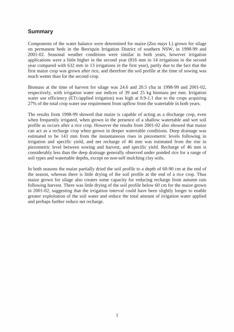
Summary Components of the water balance were determined for maize (Zea mays L) grown for silage on permanent beds in the Berriquin Irrigation District of southern NSW, in 1998-99 and 2001-02. Seasonal weather conditions were similar in both years, however irrigation applications were a little higher in the second year (816 mm in 14 irrigations in the second year compared with 632 mm in 13 irrigations in the first year), partly due to the fact that the first maize crop was grown after rice, and therefore the soil profile at the time of sowing was much wetter than for the second crop. Biomass at the time of harvest for silage was 24.6 and 20.5 t/ha in 1998-99 and 2001-02, respectively, with irrigation water use indices of 39 and 25 kg biomass per mm. Irrigation water use efficiency (ETc/applied irrigation) was high at 0.9-1.1 due to the crops acquiring 27% of the total crop water use requirement from upflow from the watertable in both years. The results from 1998-99 showed that maize is capable of acting as a discharge crop, even when frequently irrigated, when grown in the presence of a shallow watertable and wet soil profile as occurs after a rice crop. However the results from 2001-02 also showed that maize can act as a recharge crop when grown in deeper watertable conditions. Deep drainage was estimated to be 143 mm from the instantaneous rises in piezometric levels following in irrigation and specific yield, and net recharge of 46 mm was estimated from the rise in piezometric level between sowing and harvest, and specific yield. Recharge of 46 mm is considerably less than the deep drainage generally observed under ponded rice for a range of soil types and watertable depths, except on non-self mulching clay soils. In both seasons the maize partially dried the soil profile to a depth of 60-90 cm at the end of the season, whereas there is little drying of the soil profile at the end of a rice crop. Thus maize grown for silage also creates some capacity for reducing recharge from autumn rain following harvest. There was little drying of the soil profile below 60 cm for the maize grown in 2001-02, suggesting that the irrigation interval could have been slightly longer to enable greater exploitation of the soil water and reduce the total amount of irrigation water applied and perhaps further reduce net recharge.

2
3
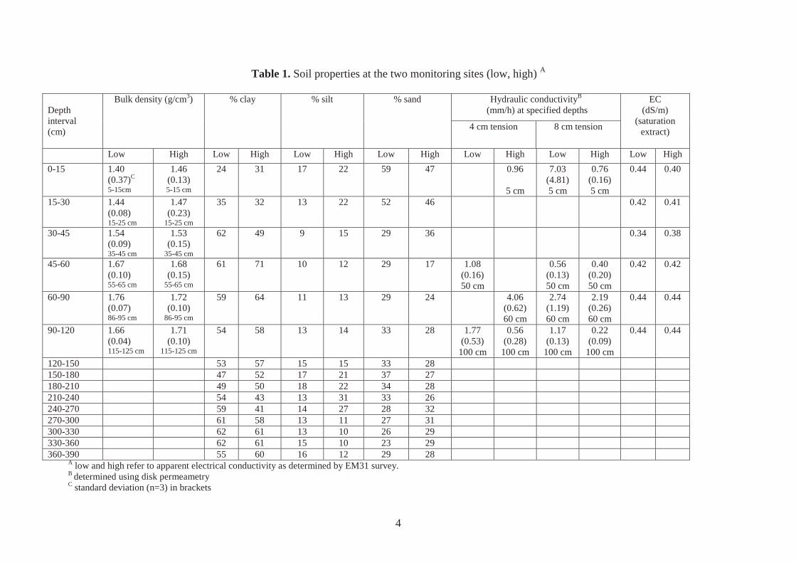
Introduction The development and implementation of Land and Water Management Plans for major irrigation areas in southern Australia commenced in the 1980s, in response to problems of rising watertables and salinisation (MDBC, 2001; McLeod, 1998). These plans have provided a set of initiatives directed primarily to control watertables and secondary salinisation through net recharge management, where net recharge is the result of recharge of the watertable (from irrigation and rain) and discharge (from lateral flow, downwards leakage, capillary upflow, plant transpiration and soil surface evaporation). However, the fate of water applied to the range of irrigated land uses across the range of site conditions and management has seldom been quantified. Increasingly, Land and Water Management Plans need to rely on water balance models of fields, farms and regions to help identify sustainable and affordable land and water management options (Khan et al., 2001). Calibration and validation of such models are critical for ensuring that guidelines and policy are soundly based, and to give policy makers and landholders the confidence to follow through to implementation. Therefore Murray Irrigation Ltd and Coleambally Irrigation Cooperative Ltd sponsored a field monitoring project with the National Program for Irrigation Research and Development (NPIRD) to determine components of the water balance, watertable behaviour and soil parameters for a range of irrigated crops including maize, winter cereals, annual pasture and lucerne (Humphreys and Edraki 2003). This report presents the findings from the determination of components of the water balance for maize grown in 1998-99 and 2001-02 in southern New South Wales. Methods Site Components of the water balance were determined for maize grown for silage in 1998-99 and 2001-02 on a 20 ha field located on a private farm 12 km NE of Finley, NSW, Australia (1450 33′ E, 350 39′ S). The soil consists of a loam or a clay loam topsoil (0-15 cm) overlying a medium to heavy clay, and is classified as a Red Brown Earth (Stace et al.1972) or Xeralf (Soil Survey Staff 1975). The local name is Tuppal or Moira loam (Evans, pers. comm.; Smith 1945). Soil properties are summarized in Table 1. Before the start of the first maize season in October 1998, the paddock grew rice in a ponded contour layout for 5 consecutive years. In mid June 1998, the paddock was ploughed, landformed and raised beds were installed. Bed width (mid-furrow to mid-furrow) was 1.5 m and the field had a grade of 1:1400 down the beds. Between March 1999 (harvest of the first maize crop) and November 2001 (sowing of the second maize crop), the paddock was sown to wheat (1999) then barley (2000). The same beds were used for all crops. The crops were irrigated by flooding the furrows using siphons from a supply channel across the top end of the field. A drainage channel at the bottom of the field removed surface drainage from the field. Prior to installation of the monitoring equipment, the field was surveyed using electromagnetic inductance (EM31) to identify the spatial distribution of the bulk soil conductivity over the profile to a depth of about 5 m (Beecher et al. 2002). EM31 values are influenced by a range of soil properties including water content, salinity and clay content, and high EM31 values are often
4
Table 1. Soil properties at the two monitoring sites (low, high) A
Hydraulic conductivityB (mm/h) at specified depths
Depth interval (cm)
Bulk density (g/cm3) % clay % silt % sand
4 cm tension 8 cm tension
EC (dS/m)
(saturation extract)
Low High Low High Low High Low High Low High Low High Low High
0-15 1.40 (0.37)C
5-15cm
1.46 (0.13) 5-15 cm
24 31 17 22 59 47 0.96
5 cm
7.03 (4.81) 5 cm
0.76 (0.16) 5 cm
0.44 0.40
15-30 1.44 (0.08) 15-25 cm
1.47 (0.23)
15-25 cm
35 32 13 22 52 46 0.42 0.41
30-45 1.54 (0.09) 35-45 cm
1.53 (0.15)
35-45 cm
62 49 9 15 29 36 0.34 0.38
45-60 1.67 (0.10) 55-65 cm
1.68 (0.15)
55-65 cm
61 71 10 12 29 17 1.08 (0.16) 50 cm
0.56 (0.13) 50 cm
0.40 (0.20) 50 cm
0.42 0.42
60-90 1.76 (0.07) 86-95 cm
1.72 (0.10)
86-95 cm
59 64 11 13 29 24 4.06 (0.62) 60 cm
2.74 (1.19) 60 cm
2.19 (0.26) 60 cm
0.44 0.44
90-120 1.66 (0.04) 115-125 cm
1.71 (0.10)
115-125 cm
54 58 13 14 33 28 1.77 (0.53)
100 cm
0.56 (0.28)
100 cm
1.17 (0.13)
100 cm
0.22 (0.09)
100 cm
0.44 0.44
120-150 53 57 15 15 33 28 150-180 47 52 17 21 37 27 180-210 49 50 18 22 34 28 210-240 54 43 13 31 33 26 240-270 59 41 14 27 28 32 270-300 61 58 13 11 27 31 300-330 62 61 13 10 26 29 330-360 62 61 15 10 23 29 360-390 55 60 16 12 29 28
A low and high refer to apparent electrical conductivity as determined by EM31 survey. B determined using disk permeametry C standard deviation (n=3) in brackets
5
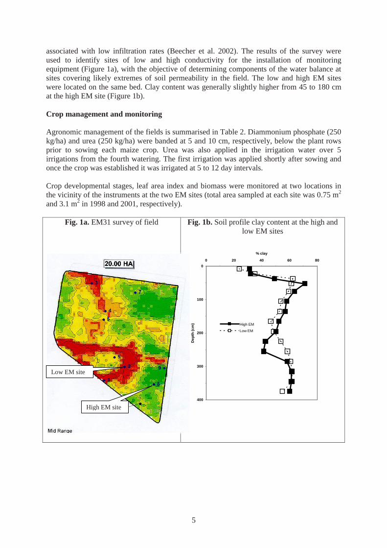
associated with low infiltration rates (Beecher et al. 2002). The results of the survey were used to identify sites of low and high conductivity for the installation of monitoring equipment (Figure 1a), with the objective of determining components of the water balance at sites covering likely extremes of soil permeability in the field. The low and high EM sites were located on the same bed. Clay content was generally slightly higher from 45 to 180 cm at the high EM site (Figure 1b). Crop management and monitoring Agronomic management of the fields is summarised in Table 2. Diammonium phosphate (250 kg/ha) and urea (250 kg/ha) were banded at 5 and 10 cm, respectively, below the plant rows prior to sowing each maize crop. Urea was also applied in the irrigation water over 5 irrigations from the fourth watering. The first irrigation was applied shortly after sowing and once the crop was established it was irrigated at 5 to 12 day intervals. Crop developmental stages, leaf area index and biomass were monitored at two locations in the vicinity of the instruments at the two EM sites (total area sampled at each site was 0.75 m2 and 3.1 m2 in 1998 and 2001, respectively).
Fig. 1a. EM31 survey of field Fig. 1b. Soil profile clay content at the high and low EM sites
0
100
200
300
400
0 20 40 60 80
% clay
Dep
th (
cm) High EM
Low EM
Low EM site
High EM site

6
Table 2. Agronomic management for the two maize seasons Management 1998-99 2001-02 Variety Date Rate Variety Date Rate Pre-sowing fertiliser
Diammonium phosphate
22 Oct 98 250 kg/ha banded at 5 cm
DAP 5 Nov 01 250 kg/ha banded at 5 cm
Urea 17 Sept 98 250kg/ha banded at 10 cm
Urea 1 Nov 01 250 kg/ha banded at 10 cm
Sowing Hycorn 75 24 Oct 98 68,000 seeds/ha 0.75 m row spacing depth 50 mm
DK 689 11Nov 01 68,000 seeds/ha 0.75 m row spacing depth 50 mm
Post sowing fertiliser
Urea Water run in 5 irrigations starting from 4th
250 kg/ha (50 kg/ha per irrigation)
Urea Water run in 5 irrigations starting from 4th
250 kg/ha (50 kg/ha per irrigation)
Pesticides /Herbicides
Atrazine, Endosulfuron
5 L/ha Atrazine 5 L/ha
7
Irrigation, surface drainage and rainfall Irrigation and drainage flows were measured with ultrasonic Starflow 1 meters. Irrigation volumes were also measured with a Dethridge meter, which was located about 1 km from the field and was read before and after each irrigation. The Starflow meters were installed inside pipes near the inlet and outlet of the field, with at least 10 pipe diameters of straight pipe upstream and 2 diameters downstream of the meters. The installations were designed so that the pipes always ran full. Data were logged at 15-minute intervals. Flow was calculated from velocity and the cross-sectional area of the pipes. Comparison of the volume of separate irrigations as measured by the Dethridge wheel and Starflow meter showed reasonable correlation between the two methods (R2>0.82), however flows determined by the Dethridge meter were generally lower than those using the Starflow meter (Figure 2). The Starflow data were used in the water balance calculations. In the second year, a new, larger drainage pipe was installed which did not run full, however the depth sensor on the Starflow meter failed, so surface runoff could not be determined. Rainfall was collected in a manual rain gauge installed adjacent to the field. Groundwater levels Piezometers were installed at the high and low EM31 sites to monitor groundwater pressure. The piezometers were not installed until after the first irrigation. These consisted of PVC (50 mm OD) pipes perforated along the bottom 0.5 m and installed to depths of 0.75 and 4 m. The piezometers were installed by augering a hole wider than the diameter of the piezometers, backfilling the hole with gravel adjacent to the perforations, then backfilling with bentonite plugs and soil to prevent artificial flow of water down the outsides of the piezometer pipes. Piezometric levels were measured manually during the first crop, and using depth (pressure level) sensors logged hourly with Dataflow loggers in the 4 m piezometers during the second crop. The shallow piezometers were not monitored during the second crop. Soil water content Soil water content was measured with Enviroscan capacitance sensors at 10, 20, 40, 60, 90 and 150 cm soil depths. Calibration of the sensors at each EM site was carried out by regressing the Enviroscan readings against volumetric soil water content determined from 10 cm diameter x 10 cm long cores taken from each monitoring depth using brass rings. Three cores were taken adjacent to the Enviroscan access tube at each sensor depth at both the low and high EM31 sites. The data from both EM31 sites and all soil layers fitted well in the one regression, therefore a single calibration equation was used for all depths and both sites (Figure 3). Soil water content was logged hourly, and the raw data were converted to volumetric soil water content and integrated over the soil profile (0-150 cm).
1 Use of registered trade names does not imply endorsement.

8
Fig. 2. Comparison of the Dethridge wheel and Starflow meter readings for each irrigation in 1998-99 and 2001-02
y = 0.81x
R2 = 0.78
0
5
10
15
20
25
30
0 5 10 15 20 25 30
Starflow (ML)
Wh
eel (
ML
)
Figure 3. Enviroscan calibration
y = 0.51x + 16.5
R2 = 0.78
0
10
20
30
40
50
60
0 10 20 30 40 50 60
Enviroscan
Vo
lum
etri
c so
il w
ater
co
nte
nt
9
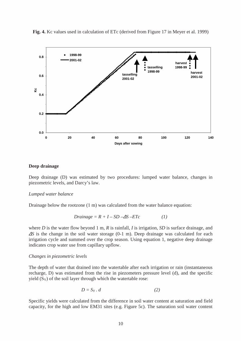
Soil water potential In November 2001, two Jet–fill tensiometers were installed at 120 and 135 cm depths at each EM 31 site and logged hourly using Hobo loggers. Manually read tube tensiometers were also installed in close proximity to (within 20-30 cm) and at the same depths as the Enviroscan sensors. Occasional readings of the tube tensiometers were made with a manual (Loktronic ) pressure transducer, and the data were used to determine the soil water characteristic with simultaneous readings of the Enviroscan sensors (Figures 5a,b,c). Unsaturated soil hydraulic conductivity Unsaturated hydraulic conductivity was determined in the major soil horizons at depths of 5, 50, 60 and 100 cm using disc permeameters (Anon. 1988). Soil pits were excavated in the vicinity of the low and high EM sites after the second maize crop was harvested, and determinations were done in triplicate at soil water potentials of -0.4 and -0.8 kPa. The methods are described in greater detail in Meister (2002). Saturated hydraulic conductivity Saturated conductivity at 4 m was determined using a slug test (Smith and Mullins 1991) in the 4 m piezometers at the low and high EM sites after harvest of the second maize crop. Weather data and reference evapotranspiration Temperature, radiation, windspeed, rainfall and humidity were logged hourly at the CSIRO Finley weather station about 12 km from the field. Reference evapotranspiration (ETo) for the period was calculated using a locally calibrated modified Penman equation (Meyer 1999). Crop evapotranspiration (ETc) was estimated from Kc x ETo, where Kc is the crop factor derived from the relationship in Figure 17 in Meyer et al. (1999), taking into account the observed LAI and date of tasselling. The Kc values used in 1998-99 are shown in Figure 4 using Kc=0.2. from sowing to 200 degree days after sowing, Kc=0.85 from 950 degree days after sowing to harvest, and linearly increasing Kc from 0.2 to 0.85 during the period from 200 to 950 degree days after sowing.
10
Fig. 4. Kc values used in calculation of ETc (derived from Figure 17 in Meyer et al. 1999)
0.0
0.2
0.4
0.6
0.8
0 20 40 60 80 100 120 140
Days after sowing
Kc
1998-99
2001-02
tasselling 1998-99
tasselling 2001-02
harvest 1998-99
harvest 2001-02
Deep drainage Deep drainage (D) was estimated by two procedures: lumped water balance, changes in piezometric levels, and Darcy’s law. Lumped water balance Drainage below the rootzone (1 m) was calculated from the water balance equation:
Drainage = R + I – SD –∆S –ETc (1) where D is the water flow beyond 1 m, R is rainfall, I is irrigation, SD is surface drainage, and ∆S is the change in the soil water storage (0-1 m). Deep drainage was calculated for each irrigation cycle and summed over the crop season. Using equation 1, negative deep drainage indicates crop water use from capillary upflow. Changes in piezometric levels The depth of water that drained into the watertable after each irrigation or rain (instantaneous recharge, D) was estimated from the rise in piezometers pressure level (d), and the specific yield (SY) of the soil layer through which the watertable rose:
D = SY . d (2) Specific yields were calculated from the difference in soil water content at saturation and field capacity, for the high and low EM31 sites (e.g. Figure 5c). The saturation soil water content
11
was determined from field observations of the maximum soil water content (immediately after irrigation) and field capacity was defined as the volumetric soil water content at 10 kPa. Results and discussion Soil hydraulic properties Soil water characteristic
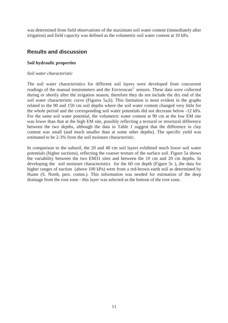
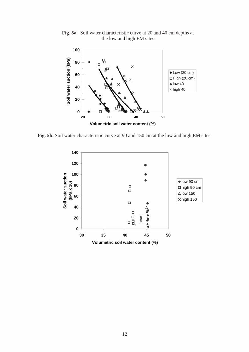
The soil water characteristics for different soil layers were developed from concurrent readings of the manual tensiometers and the Enviroscan sensors. These data were collected during or shortly after the irrigation season; therefore they do not include the dry end of the soil water characteristic curve (Figures 5a,b). This limitation is most evident in the graphs related to the 90 and 150 cm soil depths where the soil water content changed very little for the whole period and the corresponding soil water potentials did not decrease below -12 kPa. For the same soil water potential, the volumetric water content at 90 cm at the low EM site was lower than that at the high EM site, possibly reflecting a textural or structural difference between the two depths, although the data in Table 1 suggest that the difference in clay content was small (and much smaller than at some other depths). The specific yield was estimated to be 2-3% from the soil moisture characteristic. In comparison to the subsoil, the 20 and 40 cm soil layers exhibited much lower soil water potentials (higher suctions), reflecting the coarser texture of the surface soil. Figure 5a shows the variability between the two EM31 sites and between the 10 cm and 20 cm depths. In developing the soil moisture characteristics for the 60 cm depth (Figure 5c ), the data for higher ranges of suction (above 100 kPa) were from a red-brown earth soil as determined by Hume (S. North, pers. comm.). This information was needed for estimation of the deep drainage from the root zone - this layer was selected as the bottom of the root zone.
12
Fig. 5a. Soil water characteristic curve at 20 and 40 cm depths at the low and high EM sites
0
20
40
60
80
100
20 30 40 50
Volumetric soil water content (%)
So
il w
ater
su
ctio
n (
kPa)
Low (20 cm)
High (20 cm)
low 40
high 40
Fig. 5b. Soil water characteristic curve at 90 and 150 cm at the low and high EM sites.
0
20
40
60
80
100
120
140
30 35 40 45 50
Volumetric soil water content (%)
So
il w
ater
su
ctio
n(k
Pa
x 10
) low 90 cm
high 90 cm
low 150
high 150
13
Fig. 5c. Soil water characteristic curve at 60 cm at the low and high EM sites
0.01
0.10
1.00
10.00
100.00
1000.00
10000.00
20 30 40 50
Volumetric soil water content (%)
So
il su
ctio
n (
kPa)
Low
High
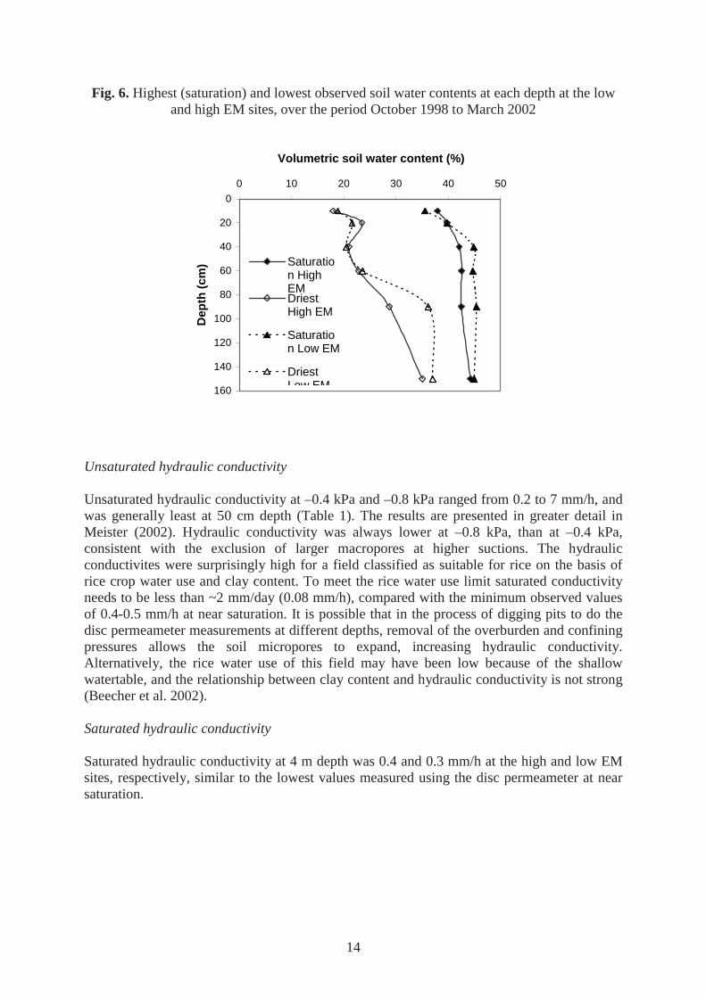
Saturation and lowest observed soil water content Soil water content profiles were constructed for the high and low EM31 sites from the maximum or minimum water observed water contents over a monitoring period of four years, which included winter (wheat, barley) and summer (maize) crops, and a long fallow between harvest of the 2000 barley and sowing of the 2001-02 maize. The maximum soil water contents represent saturation, the lower values in the topsoil reflecting the lower clay content in these layers (Figure 6). The minimum soil water contents in the upper layers to 60 cm represent the lower limit of plant water extraction. The higher minimum values below 60 cm probably reflect the influence of a shallow watertable. The similar values at both sites in respective layers are consistent with the generally similar soil properties at both sites (Table 1), suggesting that the upper 1.5 m of the soil profile at both sites was reasonably similar despite the different EM31 values.
14
Fig. 6. Highest (saturation) and lowest observed soil water contents at each depth at the low and high EM sites, over the period October 1998 to March 2002
0
20
40
60
80
100
120
140
160
0 10 20 30 40 50
Volumetric soil water content (%)
Dep
th (
cm) Saturatio
n HighEMDriestHigh EM
Saturation Low EM
Driest Low EM
Unsaturated hydraulic conductivity Unsaturated hydraulic conductivity at –0.4 kPa and –0.8 kPa ranged from 0.2 to 7 mm/h, and was generally least at 50 cm depth (Table 1). The results are presented in greater detail in Meister (2002). Hydraulic conductivity was always lower at –0.8 kPa, than at –0.4 kPa, consistent with the exclusion of larger macropores at higher suctions. The hydraulic conductivites were surprisingly high for a field classified as suitable for rice on the basis of rice crop water use and clay content. To meet the rice water use limit saturated conductivity needs to be less than ~2 mm/day (0.08 mm/h), compared with the minimum observed values of 0.4-0.5 mm/h at near saturation. It is possible that in the process of digging pits to do the disc permeameter measurements at different depths, removal of the overburden and confining pressures allows the soil micropores to expand, increasing hydraulic conductivity. Alternatively, the rice water use of this field may have been low because of the shallow watertable, and the relationship between clay content and hydraulic conductivity is not strong (Beecher et al. 2002). Saturated hydraulic conductivity Saturated hydraulic conductivity at 4 m depth was 0.4 and 0.3 mm/h at the high and low EM sites, respectively, similar to the lowest values measured using the disc permeameter at near saturation.

15
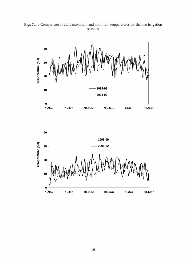
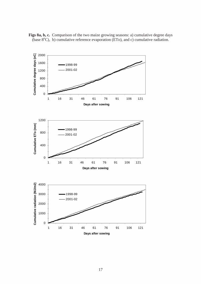
Weather Both crops received a similar amount of rain during the growing season – 81 mm in 1998-99 and 95 mm in 2001-02. However the distribution was different, with the 1998-99 crop receiving more than half the total during the early vegetative stage, and the 2001-02 crop receiving the majority of its rain during grain filling. Daily maximum and minimum temperatures during the 1998-99 irrigation season were generally higher than in 2001-02 (Figures 7a,b). However, the 1998-99 crop was planted 18 days earlier, and both crops had experienced the same cumulative mean degree days (base 8oC) or “heat units” about three months after sowing (Figure 8a). The rate of accumulation of heat units was a little lower for the 1998-99 crop during the first seven weeks, and a little higher for the remainder of the season during the grain filling period. Reference (“potential”) evaporation followed a similar pattern, and tended to be lower in 1998-99 during the first three months, and higher during grain filling, and at the end of the season the total was 7% higher during the 2001-02 season (Figure 8b). Cumulative radiation was marginally higher in the second year compared with the first year (Figure 8c).
16
Figs 7a, b Comparison of daily maximum and minimum temperatures for the two irrigation seasons
0
10
20
30
40
1-Nov 1-Dec 31-Dec 30-Jan 1-Mar 31-Mar
Tem
per
atu
re (
oC
)
1998-99
2001-02
0
10
20
30
40
1-Nov 1-Dec 31-Dec 30-Jan 1-Mar 31-Mar
Tem
per
atu
re (
oC
)
1998-99
2001-02
17
Figs 8a, b, c. Comparison of the two maize growing seasons: a) cumulative degree days (base 8oC), b) cumulative reference evaporation (ETo), and c) cumulative radiation.
0
400
800
1200
1600
2000
1 16 31 46 61 76 91 106 121
Days after sowing
Cu
mu
lati
ve d
egre
e d
ays
(oC
)
1998-99
2001-02
0
400
800
1200
1 16 31 46 61 76 91 106 121
Days after sowing
Cu
mu
lati
ve E
To
(m
m)
1998-99
2001-02
0
1000
2000
3000
4000
1 16 31 46 61 76 91 106 121
Days after sowing
Cu
mu
lati
ve r
adia
tio
n (
MJ/
m2)
1998-99
2001-02
18
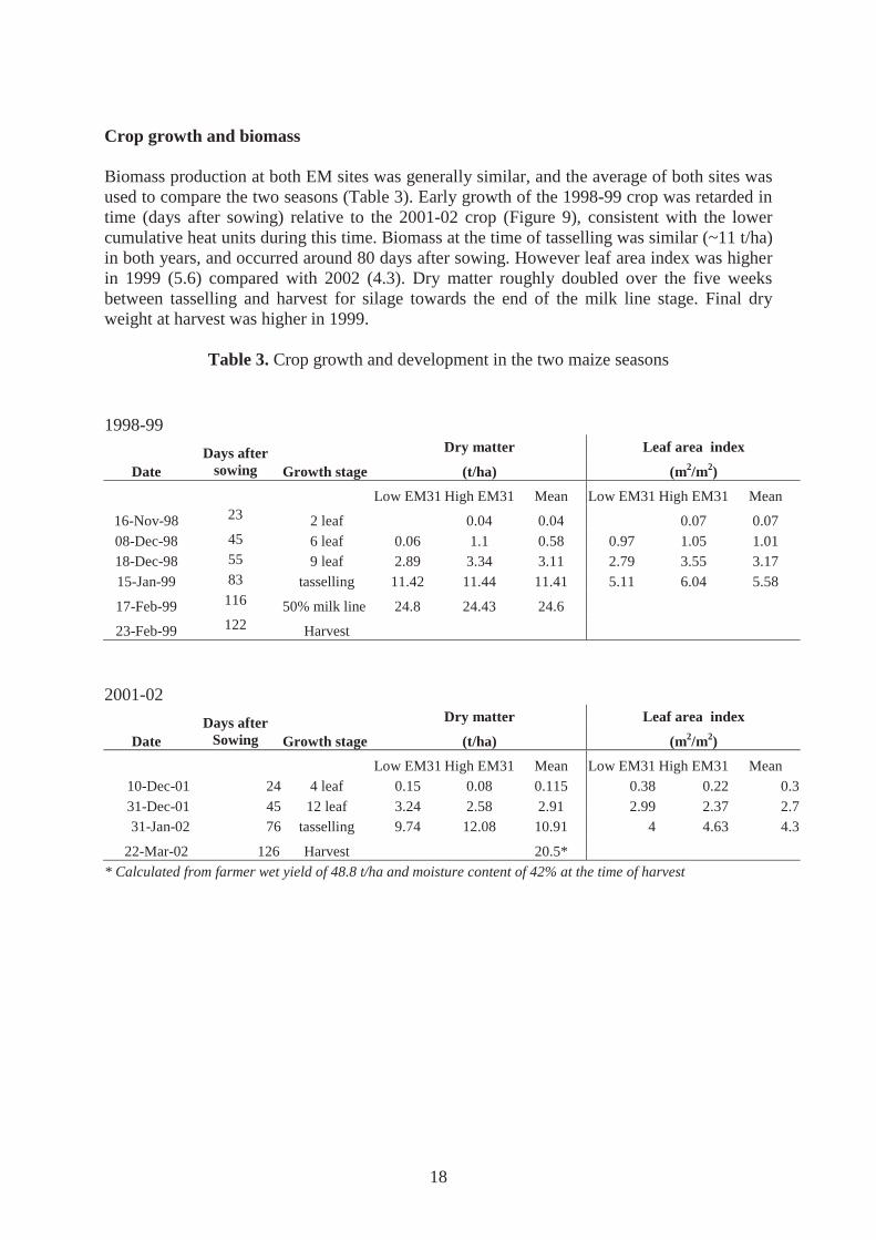
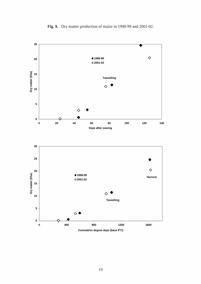
Crop growth and biomass Biomass production at both EM sites was generally similar, and the average of both sites was used to compare the two seasons (Table 3). Early growth of the 1998-99 crop was retarded in time (days after sowing) relative to the 2001-02 crop (Figure 9), consistent with the lower cumulative heat units during this time. Biomass at the time of tasselling was similar (~11 t/ha) in both years, and occurred around 80 days after sowing. However leaf area index was higher in 1999 (5.6) compared with 2002 (4.3). Dry matter roughly doubled over the five weeks between tasselling and harvest for silage towards the end of the milk line stage. Final dry weight at harvest was higher in 1999.
Table 3. Crop growth and development in the two maize seasons
1998-99 Dry matter Leaf area index
Date Days after
sowing Growth stage (t/ha) (m2/m2)
Low EM31 High EM31 Mean Low EM31 High EM31 Mean
16-Nov-98 23 2 leaf 0.04 0.04 0.07 0.07 08-Dec-98 45 6 leaf 0.06 1.1 0.58 0.97 1.05 1.01 18-Dec-98 55 9 leaf 2.89 3.34 3.11 2.79 3.55 3.17 15-Jan-99 83 tasselling 11.42 11.44 11.41 5.11 6.04 5.58
17-Feb-99 116 50% milk line 24.8 24.43 24.6
23-Feb-99 122 Harvest
2001-02 Dry matter Leaf area index
Date Days after
Sowing Growth stage (t/ha) (m2/m2)
Low EM31 High EM31 Mean Low EM31 High EM31 Mean 10-Dec-01 24 4 leaf 0.15 0.08 0.115 0.38 0.22 0.3 31-Dec-01 45 12 leaf 3.24 2.58 2.91 2.99 2.37 2.7 31-Jan-02 76 tasselling 9.74 12.08 10.91 4 4.63 4.3
22-Mar-02 126 Harvest 20.5* * Calculated from farmer wet yield of 48.8 t/ha and moisture content of 42% at the time of harvest
19
Fig. 9. Dry matter production of maize in 1998-99 and 2001-02.
0
5
10
15
20
25
0 20 40 60 80 100 120 140
Days after sowing
Dry
mat
ter
(t/h
a)
1998-99
2001-02
Tasselling
0
5
10
15
20
25
30
0 400 800 1200 1600
Cumulative degree days (base 8oC)
Dry
mat
ter
(t/h
a) 1998-99
2001-02Harvest
Tasselling
14/08/2003 20
Lumped water balance 1998-99 A total of 715 mm was applied in 13 irrigations (632 mm) plus 83 mm of rain (Table 4). Surface runoff was considerable and averaged 27% of the amount of irrigation applied, but with a much lower proportion of runoff from the first irrigation. Most irrigations were around 30-60 mm except for the first irrigation of 97 mm. The rain occurred in several small events that did not result in runoff. Net water application (546 mm) was thus 141 mm less than the estimated crop water use requirement of 687 mm. Soil water content in the 0-1 m layer was 35 mm higher at harvest than at sowing. Except for the periods between 20-26 December and 6-13 of January 1999, there was net upflow to the root zone (0-1 m) from the deeper layers as indicated by the negative values in the last column of Table 4. Net upflow over the whole season was estimated to be 176 mm from the lumped water balance, suggesting that the crop acquired a total of 176 mm from upflow from the shallow watertable, equivalent to 26% of crop water use.
Table 4. Components of the water balance for each irrigation interval in the 1998-99 season (accounting is from around midday on the first day to around midday on the last day)
Rain ∆s ETc (0-1 m)
Period (mm)
Irrigation
(mm)
Surface drainage
(mm) (mm)
Kc (mean)
ET0
(mm) (mm)
DD/UFA
(mm)
26/10/98 -03/12/98 50 97 10 59 0.28 274 77 1
03/12/98-11/12/98 58 14 15 0.48 78 38 -9 11/12/98-20/12/98 14 24 8 1 0.57 87 50 -21 20/12/98-26/12/98 2 59 16 -6 0.66 62 41 10
26/12/98-01/01/99 23 17 -24 0.72 58 42 -12
01/01/99-06/01/99 43 8 -14 0.78 63 49 0 06/01/99-13/01/99 10 61 6 -9 0.85 63 52 22
13/01/99-17/01/99 34 11 -5 0.85 46 39 -11 17/01/99-25/01/99 4 32 17 -5 0.85 82 70 -46 25/01/99-01/02/99 1 49 15 -6 0.85 65 56 -15
01/02/99-08/02/99 56 24 -10 0.85 73 62 -20
08/02/99-15/02/99 2 36 17 45 0.85 56 47 -71 15/02/99-23/02/99 0 60 6 -6 0.85 75 64 -4
Total 83 632 169 35 1083 687 -176 ADeep drainage or upflow calculated from the water balance equation (1) 2001-02 Irrigation applications were higher by 184 mm in 2001-02, despite similar rain and crop water use requirement in both years. Reference evaporation (ETo) was about 100 mm higher in the 2001-02 season compared with 1998-99, however estimated crop water use requirement (712 mm) was only 25 mm higher in 2001-02 because ETo was lower during the reproductive period (when crop factors were higher) in 2001-02 than in 1998-99. A total of 913 mm was applied in 14 irrigations (816 mm) plus 97 mm of rain (Table 5). Most irrigations were around 40-60 mm, but the first two were around 100 mm. Because of the flowmeter depth sensor failure, runoff could not be measured from irrigations. Field observations indicated that surface runoff was negligible for the first two irrigations. Nor was there any runoff from the 95 mm of rain, which
14/08/2003 21
fell in several events (maximum single event 27 mm). Very similar to the first season, the soil profile contained 36 mm more water at harvest than at sowing. The water balance calculations suggest that there was drainage (surface plus deep drainage) associated with most irrigations, with a total of 67 mm from the first two irrigations which is all attributed to drainage below 1 m as there was negligible runoff at the first two irrigations. Over the whole season there was a total of 165 mm of surface plus deep drainage, compared with –7 mm in the first season (the negative value indicating that upflow exceeded the sum of deep and surface drainage). Table 5. Components of the water balance for each irrigation interval in the 2001-02 season
(accounting is from around midday on the first day to around midday on the last day)
Period
Rain
(mm)
Irrigation
(mm)
∆S (0-1 m) (mm)
ET0
(mm)
Kc
ETc
(mm)
SurfaceA plus DD/UFB
(mm) 16/11/01 - 7/12/01 106 52 198 0.20 40 14 7/12/01 -19/12/01 101 9 122 0.32 39 53 19/12/01 -29/12/01 8 62 0 93 0.44 41 29 29/12/01 - 4/01/02 57 4 62 0.53 33 20
4/01/02 -11/01/02 44 -11 81 0.60 49 6
11/01/02 -17/01/02 50 1 69 0.67 46 3
17/01/02 -23/01/02 6 41 -3 53 0.74 39 11
23/01/02 -30/01/02 50 -2 77 0.82 63 -11
30/01/02 - 4/02/02 6 54 15 53 0.85 45 0
4/02/02 -14/02/02 25 64 -16 74 0.85 63 42
14/02/02 -27/02/02 52 54 3 104 0.85 88 15
27/02/02 - 3/03/02 51 4 31 0.85 27 20
3/03/02 -11/03/02 26 -12 69 0.85 59 -21
11/03/02 -22/03/02 56 -8 95 0.85 80 -16
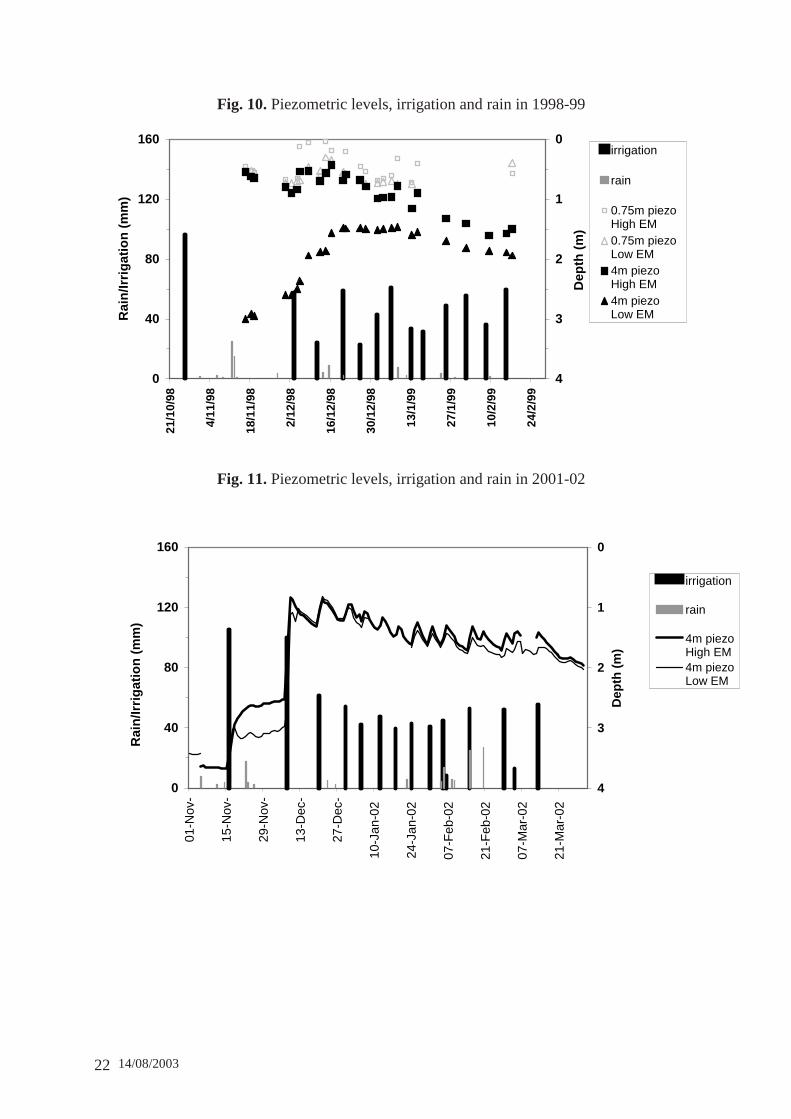
Total (net) 97 816 35 1180 712 165 A surface drainage was not measured due to flow meter failure, and is therefore included in total drainage (surface plus deep) in the lumped water balance B drainage includes both surface and deep drainage, as runoff was not measured; however, runoff was negligible at the first two irrigations Piezometric levels 1998-99 Two weeks after the first irrigation, pressure levels in all piezometers were 0.5 m below the soil surface, except for the 4 m piezometer at the low EM site which was at 3.0 m (Figure 10). We suspect that this piezometer was not in equilibrium with the surrounding groundwater due to smearing of the borehole during installation, as the pressure level was much less responsive to
14/08/2003 22
Fig. 10. Piezometric levels, irrigation and rain in 1998-99
0
40
80
120
160
21/1
0/98
4/11
/98
18/1
1/98
2/12
/98
16/1
2/98
30/1
2/98
13/1
/99
27/1
/99
10/2
/99
24/2
/99
Rai
n/Ir
rig
atio
n (
mm
)0
1
2
3
4
Dep
th (
m)
irrigation
rain
0.75m piezoHigh EM0.75m piezoLow EM4m piezo High EM4m piezo Low EM
Fig. 11. Piezometric levels, irrigation and rain in 2001-02
0
40
80
120
160
01-N
ov-
15-N
ov-
29-N
ov-
13-D
ec-
27-D
ec-
10-J
an-0
2
24-J
an-0
2
07-F
eb-0
2
21-F
eb-0
2
07-M
ar-0
2
21-M
ar-0
2
Dep
th (
m)
0
1
2
3
4
Rai
n/Ir
rig
atio
n (
mm
)
irrigation
rain
4m piezoHigh EM4m piezoLow EM
14/08/2003 23
irrigations and gradually increased over the next two months. The pressure levels in the piezometers at the low and high EM sites gradually became closer as the season progressed, with a similar rate of decline in pressure level in both piezometers from mid-January to mid-February. Both piezometers continued to exhibit similar pressure levels and responses to rain and irrigation over the next two years (data not presented) and the pressure levels and responses were very similar during the second maize crop (Figure 11). The high initial piezometric levels probably reflect a shallow watertable and high soil water content as a result of growing ponded rice in the previous season, followed by irrigation after maize sowing. From mid-December there was a general trend for pressure levels in the 4 m piezometer at the high EM site to decline despite frequent irrigation. This could have been the result of deep and lateral drainage. Crop water use from upflow from the watertable could also have contributed to the decline in the 4 m pressure levels, however this would be unlikely when there was a perched watertable present, which was frequently the case based on the fact that there was often water in the 0.75 m piezometers until mid-January and the pressure levels were higher than in the 4 m piezometer (Figure 10). There was some suggestion of piezometric responses to irrigations, but as the data were intermittent the trends were nowhere near as clear as with the logged data in the second season where there was a distinct rise in pressure level after every irrigation (Figure 11). The rate of decline in the 4 m piezometric level from the fourth irrigation to the second last irrigation was 22 mm/day, equivalent to a water depth of 0.4 mm/day for a specific yield of 2% (the porosity between saturation and field capacity). Pressure levels in the shallow (0.75 m) piezometer at the high EM site reached the surface in December 1998, and were always higher than in the 4 m piezometer (Figure 10). This indicates a downwards drainage gradient and a perched watertable, consistent with the observation of lowest minimum hydraulic conductivity and highest clay content in the subsoil horizons at the high EM site (Table 1). Pressure levels in the shallow piezometer at the low EM site were similar or slightly above those in the 4 m piezometer at the high EM site during the first two months after sowing. The shallow piezometers were dry whenever Figure 10 shows data for the 4 m piezometers and no data for the 0.75 m piezometers, which occurred from the end of January to mid-February (around the time of the fourth, third and second last irrigations). Instantaneous recharge (drainage into the watertable due to irrigation or heavy rain) can be estimated using the instantaneous rise in the watertable after each irrigation and specific yield. As the piezometers were not logged during the first season, the peak values from the manual readings probably underestimate the maximum rise in the watertable after most irrigations. Furthermore, there were no piezometer readings following the irrigation on 17 January 1999. From the second irrigation to the end of the season, instantaneous recharge below the rootzone (1 m) was calculated to be 26 mm from the rise in the piezometric levels at 4 m at the high EM site and a specific yield of 2% (Table 6). As there were no piezometer data before 16 November 1998, it was not possible to use piezometric response to estimate how much water drained to the watertable between the first irrigation in late October and the second irrigation in early December. However, based on the increase in the profile soil water content of 76 mm as a result of the 96 mm irrigation at the time of sowing, and which resulted in 10 mm runoff, we estimate that 10 mm of drainage escaped below 150 cm due to the first irrigation. Thus total deep drainage estimated from the piezometers and simple water balance for the first irrigation was estimated to be 36 mm. This may be an underestimate as it is not possible to estimate deep drainage following the 50 mm of rain that fell in 2 days mid November due to lack of piezometer data at this stage, in addition to
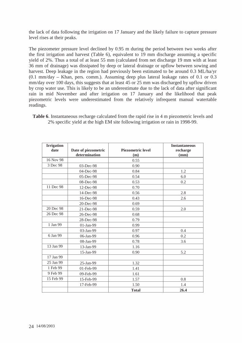
14/08/2003 24
the lack of data following the irrigation on 17 January and the likely failure to capture pressure level rises at their peaks. The piezometer pressure level declined by 0.95 m during the period between two weeks after the first irrigation and harvest (Table 6), equivalent to 19 mm discharge assuming a specific yield of 2%. Thus a total of at least 55 mm (calculated from net discharge 19 mm with at least 36 mm of drainage) was dissipated by deep or lateral drainage or upflow between sowing and harvest. Deep leakage in the region had previously been estimated to be around 0.3 ML/ha/yr (0.1 mm/day – Khan, pers. comm.). Assuming deep plus lateral leakage rates of 0.1 or 0.3 mm/day over 100 days, this suggests that at least 45 or 25 mm was discharged by upflow driven by crop water use. This is likely to be an underestimate due to the lack of data after significant rain in mid November and after irrigation on 17 January and the likelihood that peak piezometric levels were underestimated from the relatively infrequent manual watertable readings.
Table 6. Instantaneous recharge calculated from the rapid rise in 4 m piezometric levels and 2% specific yield at the high EM site following irrigation or rain in 1998-99.
Irrigation date Date of piezometric
determination Piezometric level
(m)
Instantaneous recharge
(mm) 16 Nov 98 0.55 3 Dec 98 03-Dec-98 0.90
04-Dec-98 0.84 1.2 05-Dec-98 0.54 6.0 08-Dec-98 0.53 0.2
11 Dec 98 12-Dec-98 0.70 14-Dec-98 0.56 2.8 16-Dec-98 0.43 2.6 20-Dec-98 0.69
20 Dec 98 21-Dec-98 0.59 2.0 26 Dec 98 26-Dec-98 0.68
28-Dec-98 0.79 1 Jan 99 01-Jan-99 0.99
03-Jan-99 0.97 0.4 6 Jan 99 06-Jan-99 0.96 0.2
08-Jan-99 0.78 3.6 13 Jan 99 13-Jan-99 1.16
15-Jan-99 0.90 5.2 17 Jan 99 25 Jan 99 25-Jan-99 1.32 1 Feb 99 01-Feb-99 1.41 9 Feb 99 09-Feb-99 1.61
15 Feb 99 15-Feb-99 1.57 0.8 17-Feb-99 1.50 1.4 Total 26.4
14/08/2003 25
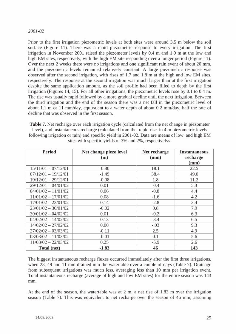
2001-02 Prior to the first irrigation piezometric levels at both sites were around 3.5 m below the soil surface (Figure 11). There was a rapid piezometric response to every irrigation. The first irrigation in November 2001 raised the piezometer levels by 0.4 m and 1.0 m at the low and high EM sites, respectively, with the high EM site responding over a longer period (Figure 11). Over the next 2 weeks there were no irrigations and one significant rain event of about 20 mm, and the piezometric levels remained relatively constant. A large piezometric response was observed after the second irrigation, with rises of 1.7 and 1.8 m at the high and low EM sites, respectively. The response at the second irrigation was much larger than at the first irrigation despite the same application amount, as the soil profile had been filled to depth by the first irrigation (Figures 14, 15). For all other irrigations, the piezometric levels rose by 0.1 to 0.4 m. The rise was usually rapid followed by a more gradual decline until the next irrigation. Between the third irrigation and the end of the season there was a net fall in the piezometric level of about 1.1 m or 11 mm/day, equivalent to a water depth of about 0.2 mm/day, half the rate of decline that was observed in the first season. Table 7. Net recharge over each irrigation cycle (calculated from the net change in piezometer
level), and instantaneous recharge (calculated from the rapid rise in 4 m piezometric levels following irrigation or rain) and specific yield in 2001-02. Data are means of low and high EM
sites with specific yields of 3% and 2%, respectivelys.
Period Net change piezo level (m)
Net recharge (mm)
Instantaneous recharge
(mm) 15/11/01 – 07/12/01 -0.80 18.1 22.5 07/12/01 – 19/12/01 -1.49 38.4 49.0 19/12/01 – 29/12/01 -0.08 1.8 11.2 29/12/01 – 04/01/02 0.01 -0.4 5.3 04/01/02 – 11/01/02 0.06 -0.8 4.4 11/01/02 – 17/01/02 0.08 -1.6 4.2 17/01/02 – 23/01/02 0.14 -2.8 3.4 23/01/02 – 30/01/02 -0.02 0.8 7.9 30/01/02 – 04/02/02 0.01 -0.2 6.3 04/02/02 – 14/02/02 0.13 -3.4 6.5 14/02/02 – 27/02/02 0.00 -.03 9.3 27/02/02 – 03/03/02 -0.11 2.5 4.9 03/03/02 – 11/03/02 -0.01 0.1 5.6 11/03/02 – 22/03/02 0.25 -5.9 2.6
Total (net) -1.83 46 143
The biggest instantaneous recharge fluxes occurred immediately after the first three irrigations, when 23, 49 and 11 mm drained into the watertable over a couple of days (Table 7). Drainage from subsequent irrigations was much less, averaging less than 10 mm per irrigation event. Total instantaneous recharge (average of high and low EM sites) for the entire season was 143 mm. At the end of the season, the watertable was at 2 m, a net rise of 1.83 m over the irrigation season (Table 7). This was equivalent to net recharge over the season of 46 mm, assuming
14/08/2003 26
specific yields of 2% at the high EM site and 3% at the low EM site. If lateral flow is negligible, upflow (UF) can be estimated from the difference between total instantaneous recharge (IR = 143 mm) and net recharge (NR = 46 mm) i.e. UF = NR-IR = -97 mm (where positive fluxes are downwards). Upflow was thus calculated as 97 mm (14% of the crop water use requirement), about half the upflow estimated from the lumped water balance in the first year. From the water balance in the second year, the sum of deep and surface drainage and upflow was 165 mm. With net recharge of 46 mm, surface drainage is calculated to be 119 mm or 15% of the total irrigation application, three-fifths of the rate of runoff (26% of the amount of irrigation) in the first year. However, this estimate of 15% irrigation runoff for the whole season is reasonable given that there was no surface drainage from the first two irrigations in the second year. From the water balance in Table 5, total surface plus deep drainage was 165 mm. Assuming 119 mm of runoff in the water balance, then there was net drainage of 46 mm below 1 m, equal to the instantaneous recharge calculated independently from the piezometric data. Soil water content 1998-99 The first three irrigations increased the soil water content at both the low and high EM sites to similar maximum values which represented saturation of the profile to at least 150 cm, and soil water content at both sites was similar during this period and during the last two irrigations (Figure 12). There appeared to be problems with the instrumentation at the low EM site between the third irrigation and the second last irrigation, with no response to irrigation, even in the shallow layers, therefore only the data for the high EM site were used in the analysis. Soil water content at the high EM site increased in response to each irrigation, but the profile was only occasionally fully saturated following irrigation, and there was a general trend for the soil water content to decline between early January and the end of the season. This is in contrast to the second season, where there was no general decline in soil water content until after the last irrigation, and most irrigations increased soil water content at the high EM site to near saturation levels (Figure 14). The fluctuations in soil water content were greatest in the upper layers (Figure 13), but the size of the response declined with time, possibly due to changes in soil physical properties. This effect was also observed in the second season in the top layer (Figure 15a). The soil water content at 150 cm was high at the time of the first irrigation, and remained high throughout the season (Figure 13). The first irrigation increased the soil water content at 90 cm to high values, and the degree of drying at this depth between irrigations increased over time, consistent with the growth of the crop and expansion of the root system and increasing crop water use from deeper layers. The soil water content at 90 cm was increased to the maximum following each irrigation (except the last two), indicating infiltration to at least 90 cm. In contrast there was almost no drying of the soil at 90 cm between irrigations during the second season (Figure 15c).
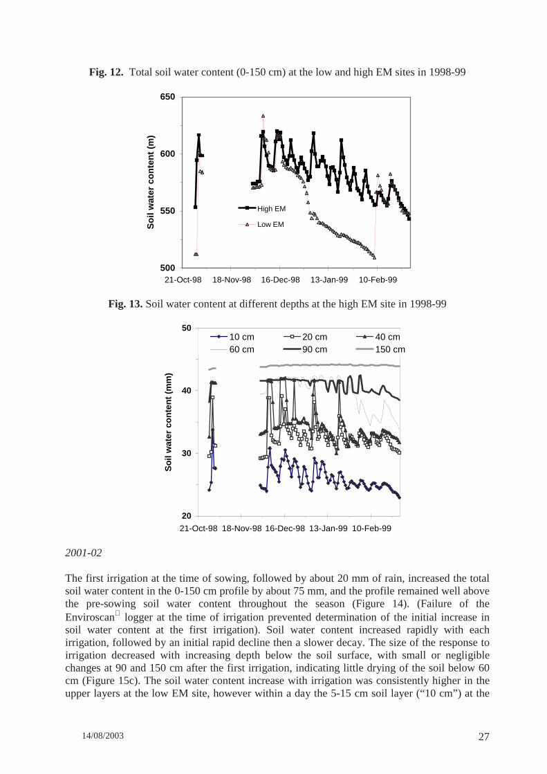
14/08/2003 27
Fig. 12. Total soil water content (0-150 cm) at the low and high EM sites in 1998-99
500
550
600
650
21-Oct-98 18-Nov-98 16-Dec-98 13-Jan-99 10-Feb-99
So
il w
ater
co
nte
nt
(m)
High EM
Low EM
Fig. 13. Soil water content at different depths at the high EM site in 1998-99
20
30
40
50
21-Oct-98 18-Nov-98 16-Dec-98 13-Jan-99 10-Feb-99
So
il w
ater
co
nte
nt
(mm
)
10 cm 20 cm 40 cm60 cm 90 cm 150 cm
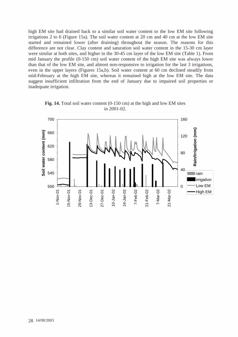
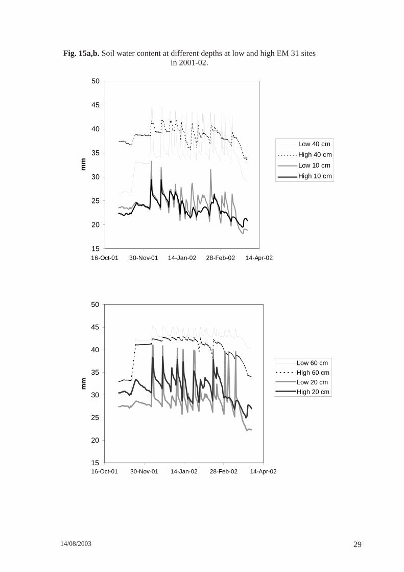
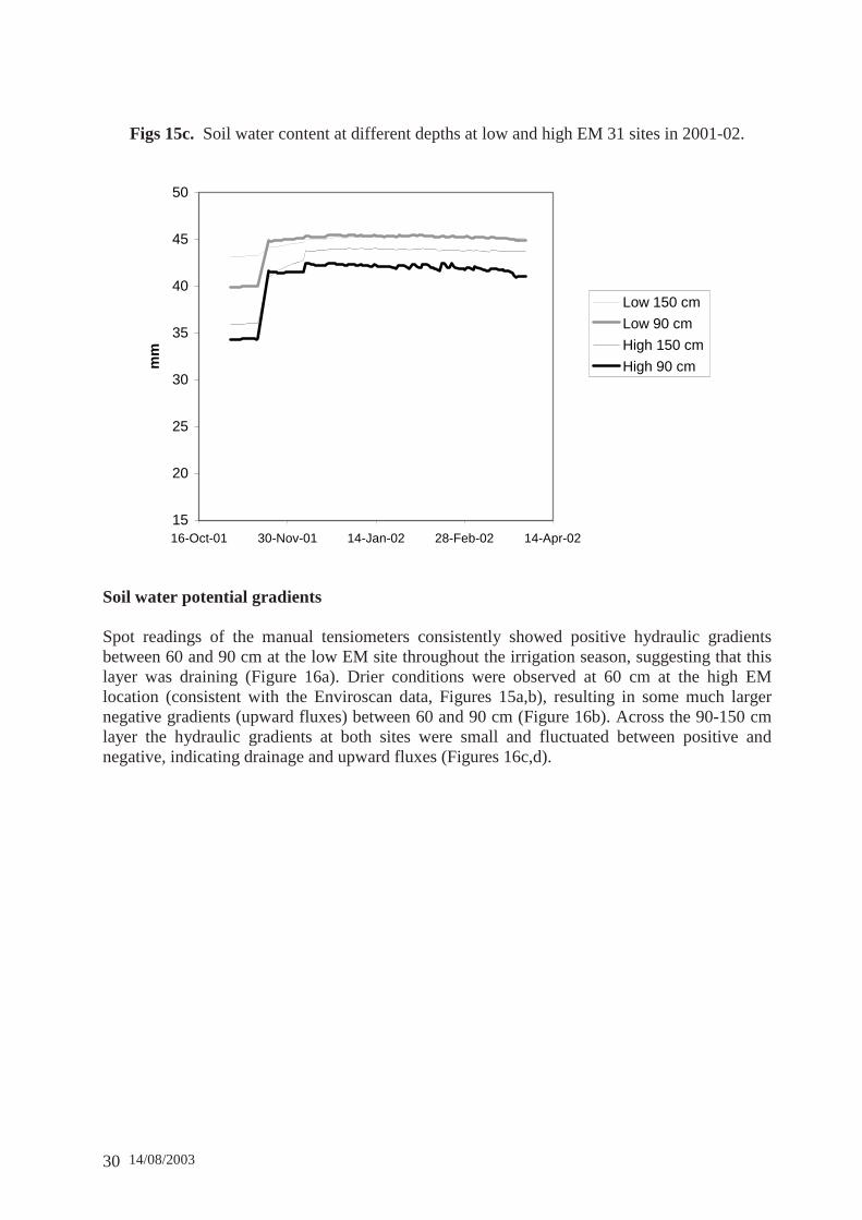
2001-02 The first irrigation at the time of sowing, followed by about 20 mm of rain, increased the total soil water content in the 0-150 cm profile by about 75 mm, and the profile remained well above the pre-sowing soil water content throughout the season (Figure 14). (Failure of the Enviroscan logger at the time of irrigation prevented determination of the initial increase in soil water content at the first irrigation). Soil water content increased rapidly with each irrigation, followed by an initial rapid decline then a slower decay. The size of the response to irrigation decreased with increasing depth below the soil surface, with small or negligible changes at 90 and 150 cm after the first irrigation, indicating little drying of the soil below 60 cm (Figure 15c). The soil water content increase with irrigation was consistently higher in the upper layers at the low EM site, however within a day the 5-15 cm soil layer (“10 cm”) at the
14/08/2003 28
high EM site had drained back to a similar soil water content to the low EM site following irrigations 2 to 6 (Figure 15a). The soil water content at 20 cm and 40 cm at the low EM site started and remained lower (after draining) throughout the season. The reasons for this difference are not clear. Clay content and saturation soil water content in the 15-30 cm layer were similar at both sites, and higher in the 30-45 cm layer of the low EM site (Table 1). From mid January the profile (0-150 cm) soil water content of the high EM site was always lower than that of the low EM site, and almost non-responsive to irrigation for the last 3 irrigations, even in the upper layers (Figures 15a,b). Soil water content at 60 cm declined steadily from mid-February at the high EM site, whereas it remained high at the low EM site. The data suggest insufficient infiltration from the end of January due to impaired soil properties or inadequate irrigation.
Fig. 14. Total soil water content (0-150 cm) at the high and low EM sites in 2001-02.
500
540
580
620
660
700
1-N
ov-0
1
15-N
ov-0
1
29-N
ov-0
1
13-D
ec-0
1
27-D
ec-0
1
10-J
an-0
2
24-J
an-0
2
7-F
eb-0
2
21-F
eb-0
2
7-M
ar-0
2
21-M
ar-0
2
So
il w
ater
co
nte
nt
(mm
)
0
40
80
120
160
Rai
n/Ir
rig
atio
n (
mm
)
rain
irrigation
Low EM
High EM
14/08/2003 29
Fig. 15a,b. Soil water content at different depths at low and high EM 31 sites in 2001-02.
15
20
25
30
35
40
45
50
16-Oct-01 30-Nov-01 14-Jan-02 28-Feb-02 14-Apr-02
mm
Low 40 cm
High 40 cm
Low 10 cm
High 10 cm
15
20
25
30
35
40
45
50
16-Oct-01 30-Nov-01 14-Jan-02 28-Feb-02 14-Apr-02
mm
Low 60 cm
High 60 cm
Low 20 cm
High 20 cm
14/08/2003 30
Figs 15c. Soil water content at different depths at low and high EM 31 sites in 2001-02.
15
20
25
30
35
40
45
50
16-Oct-01 30-Nov-01 14-Jan-02 28-Feb-02 14-Apr-02
mm
Low 150 cm
Low 90 cm
High 150 cm
High 90 cm
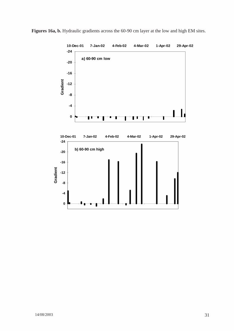
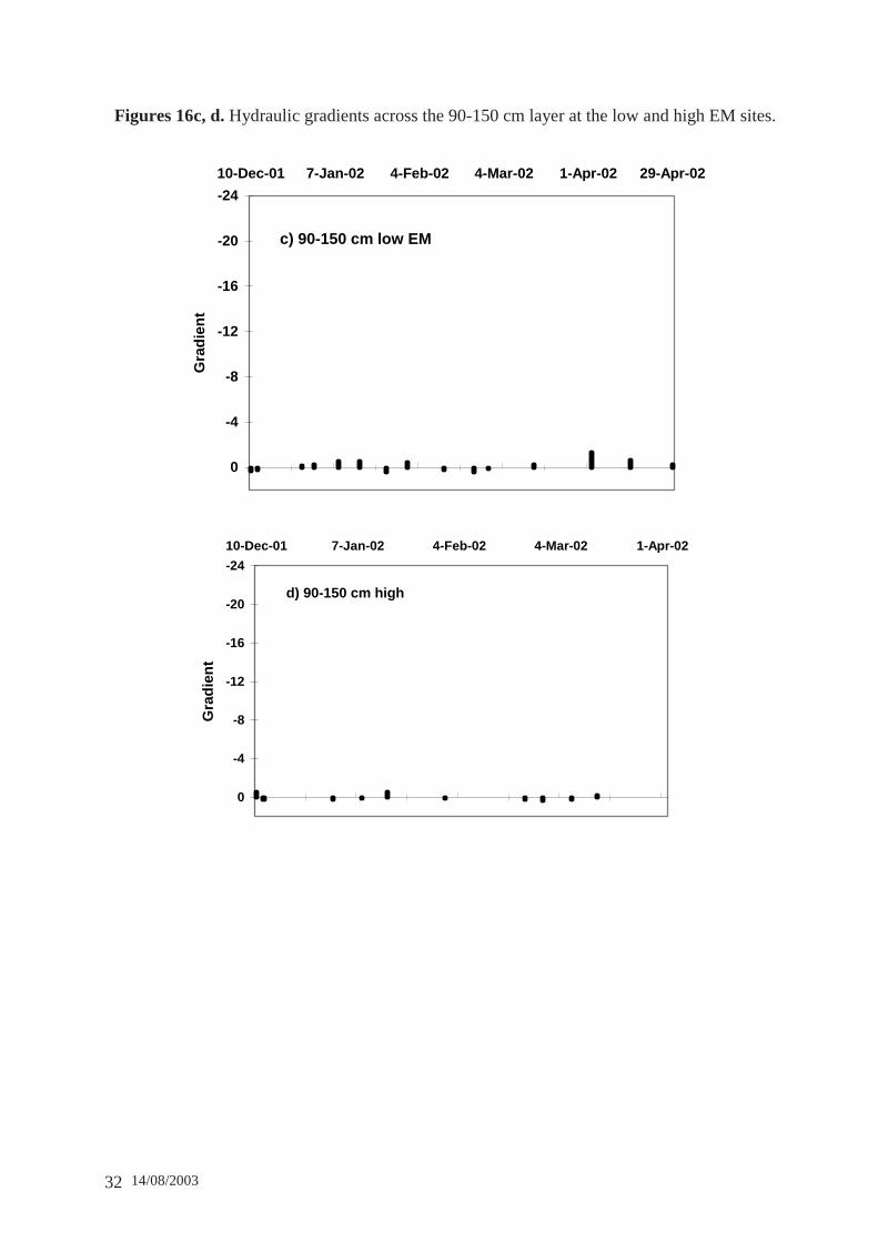
Soil water potential gradients Spot readings of the manual tensiometers consistently showed positive hydraulic gradients between 60 and 90 cm at the low EM site throughout the irrigation season, suggesting that this layer was draining (Figure 16a). Drier conditions were observed at 60 cm at the high EM location (consistent with the Enviroscan data, Figures 15a,b), resulting in some much larger negative gradients (upward fluxes) between 60 and 90 cm (Figure 16b). Across the 90-150 cm layer the hydraulic gradients at both sites were small and fluctuated between positive and negative, indicating drainage and upward fluxes (Figures 16c,d).
14/08/2003 31
Figures 16a, b. Hydraulic gradients across the 60-90 cm layer at the low and high EM sites.
-24
-20
-16
-12
-8
-4
0
10-Dec-01 7-Jan-02 4-Feb-02 4-Mar-02 1-Apr-02 29-Apr-02
Gra
die
nt
a) 60-90 cm low EM
-24
-20
-16
-12
-8
-4
0
10-Dec-01 7-Jan-02 4-Feb-02 4-Mar-02 1-Apr-02 29-Apr-02
Gra
die
nt
b) 60-90 cm high EM
14/08/2003 32
Figures 16c, d. Hydraulic gradients across the 90-150 cm layer at the low and high EM sites.
-24
-20
-16
-12
-8
-4
0
10-Dec-01 7-Jan-02 4-Feb-02 4-Mar-02 1-Apr-02 29-Apr-02
Gra
die
nt
c) 90-150 cm low EM
-24
-20
-16
-12
-8
-4
0
10-Dec-01 7-Jan-02 4-Feb-02 4-Mar-02 1-Apr-02
Gra
die
nt
d) 90-150 cm high EM
14/08/2003 33
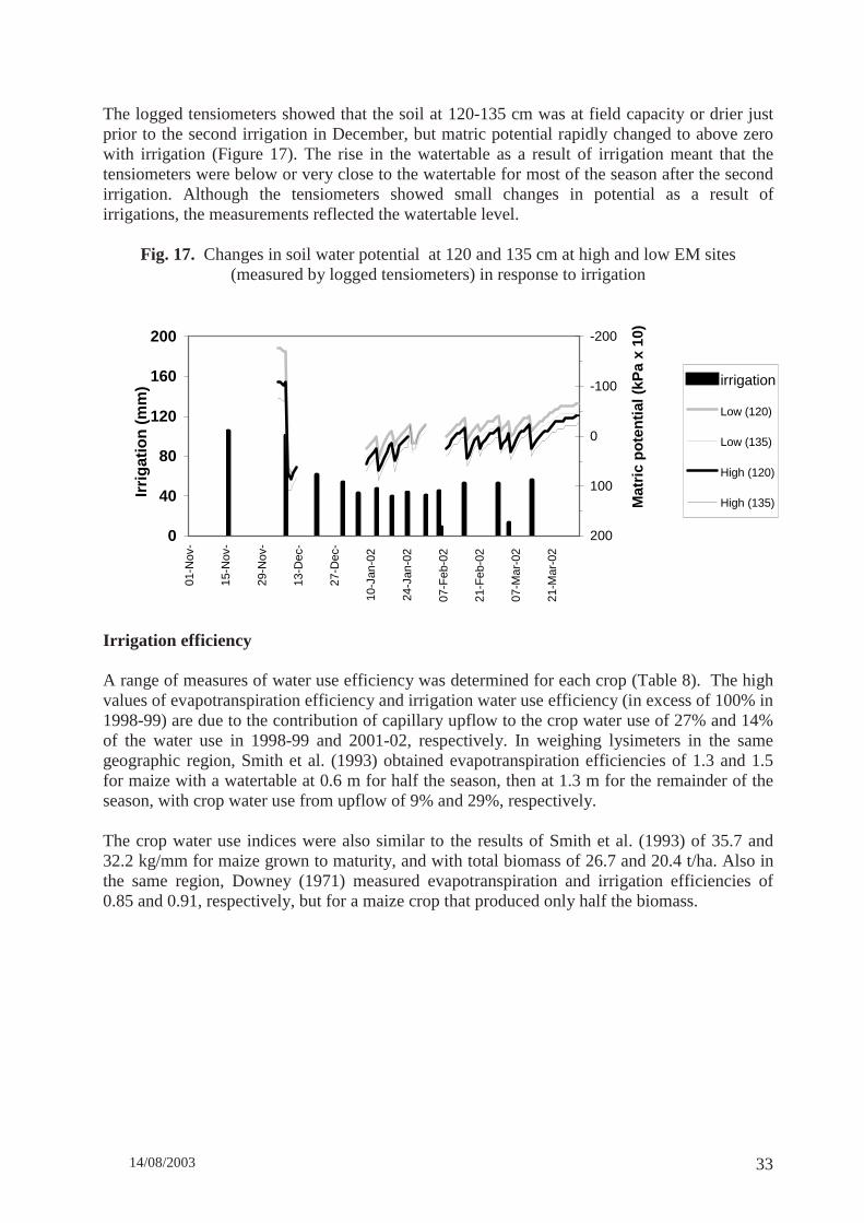
The logged tensiometers showed that the soil at 120-135 cm was at field capacity or drier just prior to the second irrigation in December, but matric potential rapidly changed to above zero with irrigation (Figure 17). The rise in the watertable as a result of irrigation meant that the tensiometers were below or very close to the watertable for most of the season after the second irrigation. Although the tensiometers showed small changes in potential as a result of irrigations, the measurements reflected the watertable level.
Fig. 17. Changes in soil water potential at 120 and 135 cm at high and low EM sites (measured by logged tensiometers) in response to irrigation
Irrigation efficiency A range of measures of water use efficiency was determined for each crop (Table 8). The high values of evapotranspiration efficiency and irrigation water use efficiency (in excess of 100% in 1998-99) are due to the contribution of capillary upflow to the crop water use of 27% and 14% of the water use in 1998-99 and 2001-02, respectively. In weighing lysimeters in the same geographic region, Smith et al. (1993) obtained evapotranspiration efficiencies of 1.3 and 1.5 for maize with a watertable at 0.6 m for half the season, then at 1.3 m for the remainder of the season, with crop water use from upflow of 9% and 29%, respectively. The crop water use indices were also similar to the results of Smith et al. (1993) of 35.7 and 32.2 kg/mm for maize grown to maturity, and with total biomass of 26.7 and 20.4 t/ha. Also in the same region, Downey (1971) measured evapotranspiration and irrigation efficiencies of 0.85 and 0.91, respectively, but for a maize crop that produced only half the biomass.
0
40
80
120
160
200
01-N
ov-
15-N
ov-
29-N
ov-
13-D
ec-
27-D
ec-
10-J
an-0
2
24-J
an-0
2
07-F
eb-0
2
21-F
eb-0
2
07-M
ar-0
2
21-M
ar-0
2
Mat
ric
po
ten
tial
(kP
a x
10)
-200
-100
0
100
200
Irri
gat
ion
(m
m) irrigation
Low (120)
Low (135)
High (120)
High (135)
14/08/2003 34
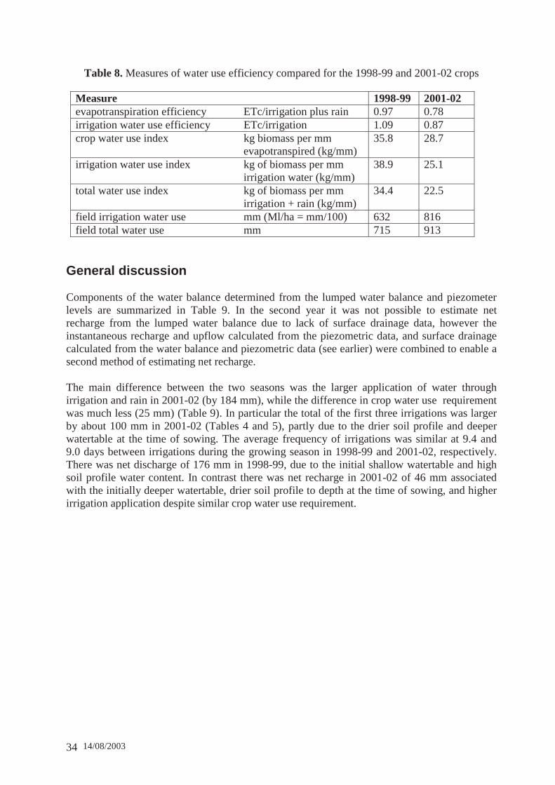
Table 8. Measures of water use efficiency compared for the 1998-99 and 2001-02 crops
Measure 1998-99 2001-02 evapotranspiration efficiency ETc/irrigation plus rain 0.97 0.78 irrigation water use efficiency ETc/irrigation 1.09 0.87 crop water use index kg biomass per mm evapotranspired (kg/mm)
35.8 28.7
irrigation water use index kg of biomass per mm irrigation water (kg/mm)
38.9 25.1
total water use index kg of biomass per mm irrigation + rain (kg/mm)
34.4 22.5
field irrigation water use mm (Ml/ha = mm/100) 632 816 field total water use mm 715 913
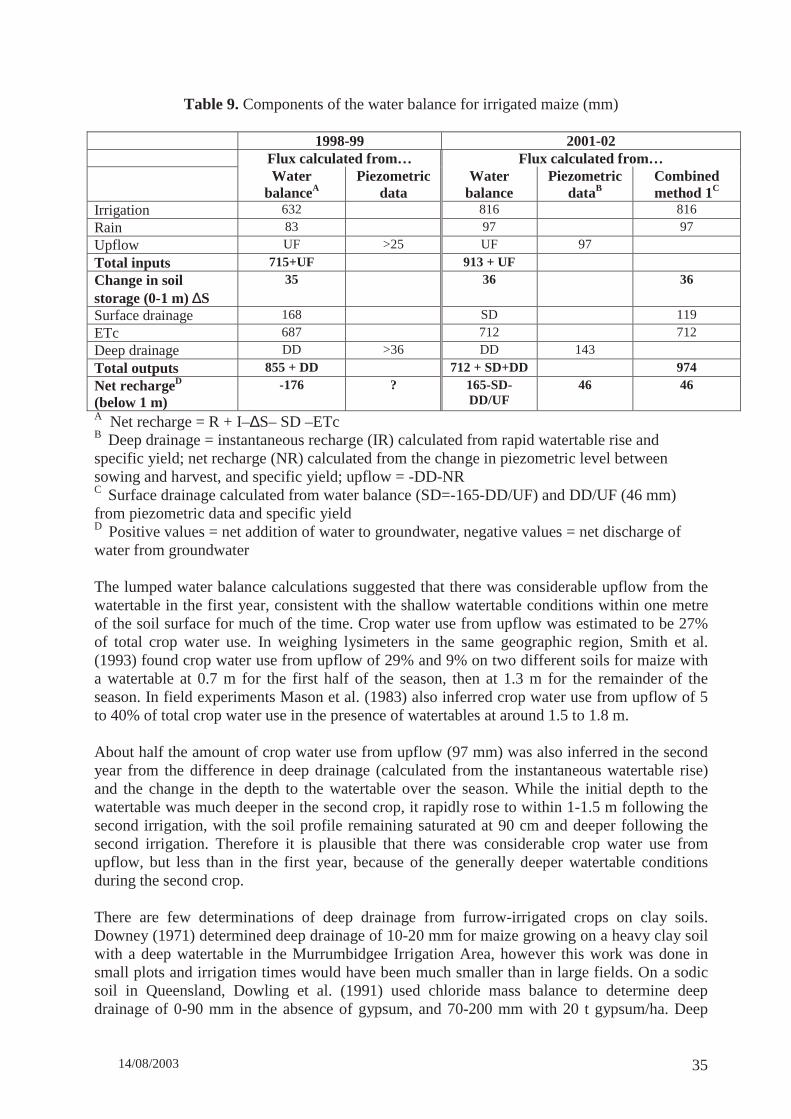
General discussion Components of the water balance determined from the lumped water balance and piezometer levels are summarized in Table 9. In the second year it was not possible to estimate net recharge from the lumped water balance due to lack of surface drainage data, however the instantaneous recharge and upflow calculated from the piezometric data, and surface drainage calculated from the water balance and piezometric data (see earlier) were combined to enable a second method of estimating net recharge. The main difference between the two seasons was the larger application of water through irrigation and rain in 2001-02 (by 184 mm), while the difference in crop water use requirement was much less (25 mm) (Table 9). In particular the total of the first three irrigations was larger by about 100 mm in 2001-02 (Tables 4 and 5), partly due to the drier soil profile and deeper watertable at the time of sowing. The average frequency of irrigations was similar at 9.4 and 9.0 days between irrigations during the growing season in 1998-99 and 2001-02, respectively. There was net discharge of 176 mm in 1998-99, due to the initial shallow watertable and high soil profile water content. In contrast there was net recharge in 2001-02 of 46 mm associated with the initially deeper watertable, drier soil profile to depth at the time of sowing, and higher irrigation application despite similar crop water use requirement.
14/08/2003 35
Table 9. Components of the water balance for irrigated maize (mm) 1998-99 2001-02 Flux calculated from… Flux calculated from… Water
balanceA Piezometric
data Water
balance Piezometric
dataB Combined method 1C
Irrigation 632 816 816
Rain 83 97 97
Upflow UF >25 UF 97
Total inputs 715+UF 913 + UF Change in soil storage (0-1 m) ∆S
35 36 36
Surface drainage 168 SD 119
ETc 687 712 712
Deep drainage DD >36 DD 143
Total outputs 855 + DD 712 + SD+DD 974 Net rechargeD (below 1 m)
-176
? 165-SD-DD/UF
46 46
A Net recharge = R + I–∆S– SD –ETc B Deep drainage = instantaneous recharge (IR) calculated from rapid watertable rise and specific yield; net recharge (NR) calculated from the change in piezometric level between sowing and harvest, and specific yield; upflow = -DD-NR C Surface drainage calculated from water balance (SD=-165-DD/UF) and DD/UF (46 mm) from piezometric data and specific yield D Positive values = net addition of water to groundwater, negative values = net discharge of water from groundwater The lumped water balance calculations suggested that there was considerable upflow from the watertable in the first year, consistent with the shallow watertable conditions within one metre of the soil surface for much of the time. Crop water use from upflow was estimated to be 27% of total crop water use. In weighing lysimeters in the same geographic region, Smith et al. (1993) found crop water use from upflow of 29% and 9% on two different soils for maize with a watertable at 0.7 m for the first half of the season, then at 1.3 m for the remainder of the season. In field experiments Mason et al. (1983) also inferred crop water use from upflow of 5 to 40% of total crop water use in the presence of watertables at around 1.5 to 1.8 m. About half the amount of crop water use from upflow (97 mm) was also inferred in the second year from the difference in deep drainage (calculated from the instantaneous watertable rise) and the change in the depth to the watertable over the season. While the initial depth to the watertable was much deeper in the second crop, it rapidly rose to within 1-1.5 m following the second irrigation, with the soil profile remaining saturated at 90 cm and deeper following the second irrigation. Therefore it is plausible that there was considerable crop water use from upflow, but less than in the first year, because of the generally deeper watertable conditions during the second crop. There are few determinations of deep drainage from furrow-irrigated crops on clay soils. Downey (1971) determined deep drainage of 10-20 mm for maize growing on a heavy clay soil with a deep watertable in the Murrumbidgee Irrigation Area, however this work was done in small plots and irrigation times would have been much smaller than in large fields. On a sodic soil in Queensland, Dowling et al. (1991) used chloride mass balance to determine deep drainage of 0-90 mm in the absence of gypsum, and 70-200 mm with 20 t gypsum/ha. Deep
14/08/2003 36
drainage rates decreased with distance down the 315 m long furrows due to reduced duration of ponding. In deep watertable situations in northern NSW, deep drainage from cotton ranged from 17-236 mm (Willis and Black 1996; Willis et al. 1997; Moss et al. 1999; Silburn and Montgomery 2001; Weaver et al. 2002). Silburn and Montgomery (2001) reviewed the results for cotton and found that deep drainage varies considerably within the cracking grey clays, and that high quantities of deep drainage were associated with saturated subsoils throughout the growing season. Our results from 1998-99 show that maize is capable of acting as a discharge crop, even when frequently irrigated, when grown in the presence of a shallow watertable and wet soil profile as occurs after a rice crop. However the results from 2001-02 also show that maize can act as a recharge crop when grown in deeper watertable conditions. Using two methods we estimate net recharge of 46 mm for maize grown under frequent furrow irrigation with an initial deep watertable in the second year. This is considerably less than the amount of deep drainage generally observed under ponded rice for a range of soil types and watertable depths, except where rice was grown on non-self mulching clay soils (Beecher et al. 2002). In both seasons the maize partially dried the soil profile down (to a depth of 60-90 cm) at the end of the season, whereas there is little drying of the soil profile at the end of the rice crop (Humphreys et al. 2001). Thus maize grown for silage also creates some capacity for reducing recharge from autumn rain following harvest. Maize grown for grain is likely to dry the soil down further as irrigations cease while there is still green leaf area, and there is a considerable drydown period between the last irrigation and harvest. In the case of silage, the maize is harvested as soon as the soil is trafficable after the last irrigation. This lends itself to the early establishment of a winter crop after harvest for silage, which is again beneficial for use of winter rain instead of allowing it to refill the soil profile and for deep drainage to continue. There was little drying of the soil profile below 60 cm for the maize grown in 2001-02, suggesting that the irrigation interval could have been slightly longer to enable greater exploitation of the soil water and perhaps further reduce net recharge. References Anon. 1988 CSIRO Disc Permeameter Instruction Manual. CSIRO Centre for Environmental
Mechanics, Canberra, ACT. Beecher, H.G., Hume, I.H. and Dunn, B.W. (2002). Improved method for assessing rice soil
suitability to restrict recharge. Aust. J. Exp. Agric. 42(3), 297-307. Dowling, A.J., Thorburn, P.J., Ross, P.J. and Ellito, P.J. (1991). Estimation of infiltration and
deep drainage ina furrow-irrigated sodic duplex soil. Australian Journal of Soil Research 29, 363-375.
Downey, L.A. (1971). Effect of gypsum and drought stress on maize ( zea mays L). II.
Consumptive use of water. Agron. J. 63, 597-600. Humphreys, E. and Edraki, M. (2003). Rigorously determined water balance benchmarks for
irrigated crops and pastures. NPIRD Project CLW21 Final Report. CSIRO Land and Water Consultancy Report.
14/08/2003 37
Humphreys, E., Bhuiyan, M., Fattore, A., Fawcett, B. and Smith, D. (2001) The benefits of winter crops after rice harvest Part 1: Results of field experiments. Farmers' Newsletter Large Area No. 157, pp.36-38.
Khan, S., Robinson, D., Xevi, E., O’Connell, N. (2001) Integrated hydrologic economic
modeling techniques to develop local and regional policies for sustainable rice farming systems. 1st Asian Regional Conference on Agriculture, Water and Environment, ICID, September 2001, Seoul, Korea.
McLeod, G.D. (1998). Achieving sustainable change-An Australian Experience . Proceedings :
Watershed Management: Moving from theory to implementation. May 3-6 ,1998. Denver , Colorado, USA
MDBC, (2001) . Review of Natural Resources Planning and implementation Processes in
selected Irrigated Regions through Australia. Volume 1, Jun 2001. Prepared by SMEC Australia Pty Ltd
Meister, N. 2002. Saturated and Unsaturated Hydraulic Conductivity of Soils in the Murray
Irrigation Area. CSIRO Land and Water Studentship Report. Griffith, NSW. Moss, J. Gordon, I., Zischke, R. (1999) Vertosols do “leak”! – water and solute movement
below irrigated cotton. In ‘Murray-Darling Basin Groundwater Workshop 1999’, Conference Proceedings, 14-16 September 1999, Griffith, NSW, Australia. pp. 298-303.
Meyer, W.S. (1999). Standard reference evaporation calculation for inland, south eastern
Australia. CSIRO Land and Water Technical Report 35/98. Meyer, W.S., Smith, D.J. and Shell, G. (1999). Estimating reference evaporation and crop
evapotranspiration from weather data and crop coefficients. CSIRO Land and Water Technical Report 34/98.
Moss, J., Gordon, I. And Zischke, R. (1999). Vertosols do “leak”! – water and solute movement
below irrigated cotton. Murray Darling Basin Groundwater Workshop 1999. Conference Proceedings. 14-16 September 1999, Griffith, NSW. Pp. 298-303.
Silburn, M. and Montgomery, J. (2001). Deep drainage under irrigated cotton in Australia – a
review (in progress). Paper presented at the Cotton Consultants Association Meeting, Dalby Qld 21022 June 2001.
Smith, R. 1945. Soils of the Berriquin Irrigation District, N.S.W. Council for Scientific and
Industrial Research Bulletin No. 189. CSIR, Melbourne, Vic. Smith, K.A. and Mullins, C.E. (eds) (1991). Soil Analysis, Physical Methods. Marcel Dekker
Inc. Smith, D.J., Meyer, W.S. and Barrs, H.D. (1993). Effects of soil type onmaize crop daily water
use and capillary upflow in weighing lysimeters during 1989/90. CSIRO Division of Water Resources Technical Report 93/20.
14/08/2003 38
Soil Survey Staff (1975). Soil Taxonomy: A Basic system of Soil Classification fro Making and Interpreting Soil Surveys. USDA Handbook 436. Washington, USA
Stace, H.C.T., Hubble, G.D., Brewer, R., Northcote, K.H., Sleeman, J.R., Mulcahy, M.J. and
Hallsworth, E.G. (1972). A Handbook of Australian Soils. Rellim Technical Publications, Glenside, SA, Australia.
Weaver, T.B., Hulugalle, N.R. and Ghadiri, H. (2002). Measuring deep drainage an nutrient
leaching under irrigated cotton. In ‘Proceedings of the 11th Australian Cotton Conference.’
Willis, T.M. and Black, A.S. (1996). Irrigation increases groundwater recharge in the
Macquarie Valley. Australian Journal of Soil Research 34. 837-847. Willis, T.M, Black, A.S., Meyer, W.S. (1997) Estimates of deep percolation beneath cotton in
the Macquarie valley. Irrig Sci. 17:141-150.