determination of angstrom’s turbidity coefficient over thailand

Renewable Energy 28 (2003) 1685–1700www.elsevier.com/locate/renene

Determination of Angstrom’s turbiditycoefficient over Thailand

S. Janjai∗, W. Kumharn, J. LaksanaboonsongDepartment of Physics, Faculty of Science, Silpakorn University, Nakhon Pathom 73000, Thailand

Received 10 October 2002; accepted 27 December 2002

Abstract

Values of the Angstrom’s turbidity coefficient,b, at 53 meteorological stations coveringThailand were determined by using three different methods. A selection of the methods wasbased on input data available at each station. It was started with the calculation ofb at NakhonPathom (13.81°N and 100.4°E) using narrow-band spectral irradiance data obtained from amulti-filter rotating shadow band radiometer. Langley’s method was employed to calculatebfrom the spectral data. The values ofb derived from this method were used as references tovalidate a method for computingb from broad-band direct irradiance proposed by Louche etal. (Solar Energy 38(2)89). It was found that this method was valid for a tropical climate.Then Louche et al.’s method was used to calculateb at meteorological stations situated atfour main cities, namely Chiang Mai (18.78°N, 98.98°E) located in the north, Ubon Rach-athani (15.25°N, 104.87°E) in the northeast, Songkhla (7.20°N, 100.60°E) in the south andBangkok in the central region. Based on values ofb of these cities, a new model relatingbto visibility, suitable for the tropical climate was developed. This model was used to estimateb at the other 48 meteorological stations where the visibility was routinely observed. Finally,seasonal variations ofb were investigated. It was found that for the stations in the north, thenortheast and the central region, the values ofb are relatively high in the dry season(November–April). They decrease in the wet season (May–October). For most stations in thesouth,b was relatively low and remained nearly constant all year round. It was also inferredthat the northeast monsoon and the southwest monsoon had a strong influence on the seasonalvariations ofb. 2003 Elsevier Science Ltd. All rights reserved.

Keywords: Atmospheric turbidity; Angstrom’s turbidity coefficient; Aerosols

∗ Corresponding author. Tel.:+66-34-270761; fax:+66-34-271189.E-mail address: [email protected] (S. Janjai).

0960-1481/03/$ - see front matter 2003 Elsevier Science Ltd. All rights reserved.doi:10.1016/S0960-1481(03)00010-7

1686 S. Janjai et al. / Renewable Energy 28 (2003) 1685–1700

1. Introduction

The presence of aerosols in the earth’s atmosphere has important effects on thetransmission of solar radiation and the radiative heat transfers in the atmosphere.This is due to the fact that aerosols absorb and scatter solar radiation as it passesthrough the atmosphere. The absorption of solar radiation by aerosols increases theradiative heating of the atmosphere and decreases the solar energy available at theearth’s surface. To model a heat budget of the atmosphere and the solar radiationreaching the earth’ s surface, information on the amounts and properties of aerosolsis usually required [1–4]. Although the amount of aerosols presented in the atmos-phere in the vertical direction can be quantified in terms of the number of particlesper unit volume, existing techniques for determining this number is practically appli-cable only for aerosols presented near the earth’s surface. As aerosols make theatmosphere turbid, it is more common to quantify the presence of aerosols by anindex of turbidity. During the last century, some indices of turbidity were proposedand several methods were developed to determine their values [5–7]. Among theseindices, Angstrom’s turbidity coefficient, b, is one of the most widely used indicesbecause it represents the combined effects of both scattering and absorption causedby aerosols. In addition, it also indicates the amounts of aerosols. Therefore, a greatdeal of efforts have been undertaken to determine b in many countries [8–20]. How-ever, investigations of the atmospheric turbidity in the tropics are still very limited.In the case of Thailand, the only existing data of the atmospheric turbidity are thoseinvestigated by Exell [21] in the late 1970s. However, these data which are presentedin terms of Schuepp’s turbidity coefficient were derived only for two locations,namely Bangkok and Chiang Mai using broad-band solar radiation estimated 25years ago. During the last 20 years, environments in Thailand have rapidly changed.Therefore, more investigations on the atmospheric turbidity in terms of the numbersof locations and the update of data are still warranted.

To meet this demand, we proposed to determine the values of Angstrom’s turbiditycoefficient (b) at 53 meteorological stations located in every region of Thailand,based on a new data set and validated methods. In addition, we proposed to establisha new empirical model relating b to visibility, suitable for tropical climate. As alllocations under this study are situated in the tropics, seasonal variations of b affectedby monsoons and rains were also subjected to this investigation.

2. Methods

In this work, three methods were used to determined Angstrom’s turbidity coef-ficient (b) for different locations in Thailand. These methods are: (a) a calculationof b based on narrow-band spectral irradiance; (b) a derivation of b from broad-band direct irradiance; and (c) an estimation of b from visibilities. The selection ofthe methods for each location depends on the primary data available for that location.Details of calculations of each method are described as follows.

1687S. Janjai et al. / Renewable Energy 28 (2003) 1685–1700

2.1. Calculation of b from narrow-band spectral solar irradiance

This method which requires spectral irradiance data was used for determining bat Silpakorn University in Nakhon Pathom (13.81 °N, 100.4 °E) located in the Cen-tral Region of Thailand. The spectral data were obtained from a multi-filter rotatingshadow-band radiometer (MFR) of Yankee Environment System, Inc (ModelMFRSR1). This instrument was newly designed to measure a solar spectrum witha high accuracy. The band-width of each channel of the instrument is 10 nm. Theadvantage of this instrument to acquire b is that accuracies of the calculations areindependent of calibrations of the instrument. The functional principle of this instru-ment is described in [22].

The instrument was installed on the roof of the Physics Department building ofSilpakorn University in Nakhon Pathom. Global, diffuse and direct spectralirradiance at the wavelengths of 415, 500, 515, 675, 865, 940 nm were measuredfrom June 1998 to December 2000 with a sampling time interval of 24 s. Only thedirect normal spectral irradiance at the wavelength of 415 and 500 nm on clear dayswas selected to compute b. These wavelengths were chosen because absorptions byatmospheric gases and water vapour are negligible at these wavelengths. The calcu-lation of b was based on Langley’ s method [23]. According to this method, directnormal spectral irradiance at the earth’s surface (In) for a clear sky is expressed as:

Inl � Ionexp[�(t�al � t�Rl � t�wl � t�ozl � t�gl)ma] (1)

where Ion is the extraterrestrial irradiance; ma is the relative air mass;t�al,t�Rl,t�wl,t�ozl and t�gl are the optical thicknesses due to the aerosol absorptionand scattering, the Rayleigh scattering, the water vapour absorption, the ozoneabsorption and other gas absorptions, respectively. Rewriting Eq. (1) in a logarithmicform, one obtains

lnInl � lnIon�(t�al � t�Rl � t�wl � t�ozl � t�gl)ma (2)

When the values of lnInl are plotted against ma, a straight line with a slope s isobtained. This slope is equal to a sum of the various optical thicknesses as follows:

s � �(t�al � t�Rl � t�wl � t�ozl � t�gl). (3)

Since at the wavelengths of 415 nm and 500 nm, the absorption due to watervapour, ozone and other gases is negligible, the slope s is reduced to

s � �(t�al � t�Rl) (4)

with the value of the Rayleigh optical thickness (t�Rl) calculated from a formulaproposed by Leckner [24] and the value of the slope s, the aerosol optical thicknesst�al is finally determined from eq. (4). This aerosol optical thickness is related tothe Angstrom’s turbidity coefficient (b) and the wavelength exponent (a) throughthe following formula proposed by Angstrom [5].

t�al � bl�a (5)

Applying eq. (5) to the computation of aerosol optical thickness at l1 = 415


nm and l2 = 500 nm, one obtains equations relating b and a to the aerosol opticalthickness as follows :

a �

ln(t�al1

t�al2)

ln(l2

l1)

(6)

and

b �t�al1

l�a1

or b �t�al2

l�a2

(7)

where t�al1, and t�al2 are the aerosol optical thicknesses at l1 and l2, respectively.As the slope s is not varied with a calibration factor of the instrument, the accuracyof b is independent of the instrument calibration.

We applied Langley’s method to calculate b and a at Nakhon Pathom using thespectral data collected from June 1998–January 2000. Daily values of b obtainedfrom this method were averaged over a month. The results are shown in the nextsection.

2.2. Computation of b from broad-band direct solar irradiance

Although the determination of b from solar spectrum using MFR is considered tobe the most accurate methods, the equipment for measuring the spectrum is extremelyexpensive. In Thailand, the data from MFR are available only for Nakhon Pathom.One of the alternatives is to use broad-band direct irradiance to compute b. Duringthe past 20 years, a number of methods for computing b from broad-band irradiancehave been developed [20,25]. In our work, a method proposed by Louche et al. [25]was selected to compute b, due to its simplicity and acceptable accuracy. Accordingto this method, direct normal irradiance for a clear sky is expressed as

In � kE0IsctatRtwtoztg (8)

where E0 is the earth’s orbit eccentricity correction factor; Isc is the solar constant(1367 W/m2); k is a factor whose value depends on the range of solar radiationspectrum used in the calculation; ta,tR,tw,toz and tg are the transmittance due to theaerosol absorption and scattering, the Rayleigh scatting, the water vapour absorption,the ozone absorption and other gas absorptions, respectively.

The Rayleigh scattering transmittance is given by [24]:

tR � exp[�0.0903m0.84a (1.0 � ma�m1.01

a )]. (9)

ma is a relative air mass which is expressed as

ma � mr(p /p0) (10)

where mr is the air mass at the standard pressure (p0) and p is the atmosphericpressure. mr is calculated by the formula of Kasten [26] as


mr � [cosqZ � 0.15(93.885�qZ)�1.253]�1 (11)

where qZ is a zenith angle.The transmittance due to the ozone absorption is expressed as [27]

tOZ � 1�[0.1611lmr(1.0 � 139.48lmr)�0.3035 �0.002715lmr(1.0 (12)

� 0.044lmr � 0.0003(lmr)2)�1]

where l is the total amount of ozone.The transmittance due to water vapour absorption is calculated by the following

formula [27]

tw � 1�2.4959wmr[1.0 � (79.034wmr)0.6828 � 6.385wmr]�1 (13)

where w is precipitable water.The transmittance by other gases is given as follows [25]:

tg � exp(�0.0127m0.26a ) (14)

The aerosol transmittance, ta, is related to Angstrom’s turbidity coefficient, b,through a formula purposed by Machler and Iqbal [28] as

ta � (0.12445a�0.0162) � (1.003�0.125a) � exp[�bma(1.089a (15)

� 0.5123)]

Substituting ta,tR,tw,toz and tg from eqs. (9)–(15) into eq. (8), an expression forb is obtained as follows:

b �1

maDln (

CA�B

) (16)

where

A � In / (kE0IsctRtwtoztg) (17)

B � 0.1244a�0.0162 (18)

C � 1.003�0.125a (19)

D � 1.089a � 0.5123. (20)

The values of a is assumed to be 1.3, and k = 0.957 corresponding to wavelengthband of the pyrheliometer used in this work.

As Louche et al.’s method was developed from data of the mid-latitude climate,its validity for the tropics should be investigated. To accomplish this, the methodwas used to calculate b at Silpakorn Univesity in Nakhon Pathom where the solarspectrum and direct normal irradiance are parallely measured at the same place. Thedirect normal irradiance was measured with a NIP Eppley pyrheliometer and thesolar spectrum was monitored with a MFR as described in the preceding section.The ozone amounts measured in Bangkok situated approximately 60 km from Nak-hon Pathom were used for the calculations. Perceptible water was computed from


the ambient temperature and relative humidity recorded at Silpakorn University,based on a formula of Leckner [24]. As values of Angstrom’s turbidity coefficientobtained from the spectral data (bspectral) with MFR were considered to be the mostaccurate values, they were used as references to compare with those calculated fromLouch et al.’s method (bdirect), as shown in Fig. 1. It was found that for most cases,bdirect agreed well with bspectral.

After validation, this method was used to calculate Angstrom’s turbidity coef-ficient from direct normal irradiance derived from global and diffuse irradiance meas-ured at Chiang Mai located in the north, Ubon Ratchathani in the northeast, Songkhlain the south and Bangkok in the central region of the country. For Chiang Mai, UbonRatchathani and Songkhla, a 5-year period (1996–2000) of irradiance data were used.For Bangkok, the data of the year 2000 were employed to calculate b. Perceptiblewater was computed from the temperature and relative humidity measured at thesame stations. As ozone amount changes slightly for the range of latitudes of Thai-land [29], their values of Bangkok were still used for all calculations. Only clearsky irradiance was selected as input data. The identification of clear days was basedon visual inspections and cloud cover data observed at the same stations. Applyingall these data to Eqs.(9)–(20), daily values of Angstrom’s turbidity coefficient wereobtained. These values were again averaged over a month. The results are shown inSection 3.

2.3. Estimation of b from visibility data

Although direct irradiance data can be effectively used to determine b, these dataare available only at main meteorological stations in Thailand. To determine b at

Fig. 1. Comparison between Angstrom’s turbidity coefficient calculated from broad-band directirradiance (bdirect) and those obtained from narrow-band spectral irradiance (bspectral).The dotted line rep-resents a reference for the case that bdirect is equal to bspectral.


other meteorological stations for which irradiance data are not available, we proposedto estimate b from visibility data, which are commonly observed. Although someinvestigators [30,31] have proposed models relating Angstrom’s turbidity coefficient,b to visibility, these models were usually based on the climatic conditions of NorthAmerica or Europe whose visibility varies in a wide range, such as 5–100 km. ForThailand situated in the tropics, the visibility varies only in the range of 5–15 km[32]. Therefore, in this study, a correlation between b and visibility was again investi-gated, using the values of b of Chiang Mai, Ubon Ratchathani, Songkhla and Bang-kok obtained from the preceding section and the visibility data observed at the sameperiods and stations. Results obtained from this investigation are shown in Fig. 2.The correlation was then fitted with a regression equation. The best-fitted regressionequation is written as follows:

b � 0.589�0.068(VIS) � 0.0019(VIS)2 (21)

where VIS is the visibility in km.Then this model was used to estimate Angstrom’s turbidity coefficient at the other

48 meteorological stations located in all main regions of the country. Monthly-aver-aged daily values of b based on a 5-year period (1996–2000) of visibility data areshown in the following section.

3. Results and discussion

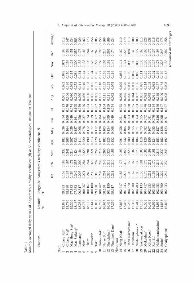
Monthly-averaged values of Angstrom’s turbidity coefficient, b, at 53 metorolog-ical stations using the methods described in the preceding section are listed in Table

Fig. 2. Correlation of Angstrom’s turbidity coefficient (b) and visibility (VIS).


1. To understand these results, it is necessary to know a climate of the country,which is explained as follows.

Thailand is situated in south-east Asia, with latitude between 5°37� N–20°27� Nand the longitude between 97°22� S–105°37� S, as shown in Fig. 3. The country canbe divided into four main regions, namely the north, the northeast, the central regionand the south. The north is partly mountainous. The northeast is a high plain withmountains in the west and the south of the region. The central region is mainly flatwith some mountains in the west and with the Gulf of Thailand in the south of theregion. The south is a peninsula with the Andaman Sea in the west and the Gulf ofThailand in the east.

According to Koppen’s classification [33], the country has a tropical climate withsubcategories Aw (tropical grass land climate), Am (tropical monsoon climate) andAf (tropical rain forest climate). The subcategory Aw is for the north, the northeastand most parts of the central region. The subcategories Am is for the eastern partof the central region and most parts of the south, except the eastern parts of thesouth which is in the subcategory Af. The climate of the country is dominated bythe northeast monsoon (November–February) and the southwest monsoons (May–October). The southwest monsoon blows during May–October from the AndamanSea to the country, causing a cloudy sky and rainfall in the whole country. Therefore,for the north, the northeast and the central region, the period (May–October) of thesouthwest monsoon is generally called the wet season. The northeast monsoon blowsfrom central Asia to the country during November to February. This monsoon bringsrelatively cold and dry air to the north, the northeast and the central region. As ittravels across the Gulf of Thailand to the south, the northeast monsoon causes rainfallin this region. Therefore, the south has a longer period of the wet season whichgenerally lasts until December or January. In the period between the two monsoonsor the summer (March–April), temperature in all regions of the country increasesdue to an increase of the incident solar radiation. There is still little rainfall in everyregion in this period. Therefore, for the north, the northeast and the central region,the period of 6 months (November–April) with little rainfall is commonly called thedry season.

This climate of the country strongly influences seasonal variations of the atmos-pheric turbidity. This phenomenon is evident from the seasonal variations of b shownin Table 1. Figs. 4–7 illustrate typical seasonal variation of b for the north, thenortheast, the central region and the south.

From Table 1, it is observed that, for most cases in the north, the northeast andmost parts of the central region, values of b reach a maximum in January, February,March or April, depending on the stations and slowly decrease to reach a minimumin June or July. Then they gradually increase again to complete an annual cycle. Inaddition, the periods of high values and low values of b correspond to the dry seasonand the wet season, respectively. This seasonal variation may be explained from thefact that during the first period of the dry season (October–February), the northeastmonsoon which is the wind of a continental origin circulates through these regions.This wind is loaded with dust particles from soils, thus increasing the atmosphericturbidity. For the second period of the dry season (March–April) air temperature

1693S. Janjai et al. / Renewable Energy 28 (2003) 1685–1700T

able

1M

onth

lyav

erag

edda

ilyva

lues

ofA

ngst

rom

’stu

rbid

ityco

effic

ient

(b)

at53

met

eoro

logi

cal

stat

ions

inT

haila

nd

Stat

ions

Lat

itude

Lon

gitu

deA

mgs

trom

’stu

rbid

ityco

effic

ient

,b

°N°E

Jan

Feb

Mar

Apr

May

Jun

Jul

Aug

Sep

Oct

Nov

Dec

Ave

rage

Nor

th1

Chi

ang

Rai

c19

.883

99.8

330.

158

0.18

30.

332

0.18

20.

036

0.01

40.

033

0.06

10.

082

0.08

90.

071

0.10

80.

112

2C

hian

gM

aib

18.7

8098

.980

0.13

50.

167

0.24

10.

205

0.16

40.

100

0.07

00.

106

0.13

00.

150

0.15

40.

153

0.14

73

Mae

Hon

gSo

nc19

.300

97.8

330.

164

0.17

10.

314

0.20

70.

059

0.04

90.

074

0.08

00.

093

0.11

50.

126

0.15

10.

134

4M

aeSa

rian

gc18

.167

97.9

330.

342

0.35

50.

424

0.33

30.

187

0.16

10.

195

0.20

30.

252

0.28

40.

300

0.35

70.

283

5L

ampa

ngc

18.2

8399

.517

0.20

50.

202

0.18

40.

111

0.06

80.

050

0.05

90.

070

0.11

10.

161

0.15

50.

175

0.12

96

Nan

c18

.767

100.

767

0.27

10.

284

0.32

90.

220

0.07

60.

037

0.05

60.

086

0.11

00.

144

0.15

80.

185

0.16

37

Phar

ec18

.167

100.

167

0.24

50.

264

0.28

10.

190

0.11

20.

074

0.08

30.

100

0.13

30.

177

0.19

30.

244

0.17

38

Utta

rado

tc17

.617

100.

100

0.29

30.

328

0.32

10.

213

0.07

70.

019

0.05

70.

065

0.09

50.

124

0.12

30.

160

0.15

69

Tak

c16

.883

99.1

500.

318

0.29

20.

256

0.22

00.

112

0.06

70.

082

0.09

50.

107

0.17

80.

227

0.26

90.

185

10Ph

itsan

ulok

c16

.783

100.

267

0.23

70.

233

0.21

60.

171

0.12

00.

084

0.09

40.

101

0.11

00.

127

0.16

80.

196

0.15

511

Nm

aeSo

tc16

.667

98.5

500.

251

0.24

60.

260

0.18

20.

103

0.08

10.

104

0.11

10.

123

0.15

80.

165

0.21

40.

166

12Ph

etch

abun

c16

.433

101.

150

0.31

00.

318

0.32

00.

225

0.13

40.

099

0.10

90.

111

0.12

50.

132

0.18

20.

205

0.18

913

Phum

ipol

Dam

c17

.250

99.0

170.

211

0.21

00.

188

0.13

20.

068

0.04

90.

054

0.06

20.

078

0.11

60.

145

0.17

40.

124

Nor

th-e

ast

14N

ong

Kha

ic17

.867

102.

717

0.18

80.

175

0.19

30.

091

0.05

80.

051

0.06

50.

066

0.07

60.

086

0.11

40.

160

0.11

015

Loe

ic17

.450

101.

733

0.27

70.

310

0.35

30.

242

0.10

50.

049

0.05

20.

075

0.12

60.

155

0.17

40.

225

0.17

916

Ubo

nR

acha

than

ib15

.250

104.

870

0.10

80.

155

0.22

30.

200

0.09

00.

053

0.07

00.

076

0.09

00.

100

0.09

60.

094

0.11

317

Udo

ntha

nic

17.3

8310

2.80

00.

162

0.16

80.

182

0.10

40.

055

0.03

80.

035

0.04

40.

080

0.08

70.

106

0.14

30.

100

18N

akho

npha

nom

c17

.417

104.

783

0.10

30.

138

0.17

30.

104

0.07

10.

064

0.08

30.

087

0.10

60.

088

0.09

30.

122

0.10

319

Sakh

onna

khon

c17

.150

104.

133

0.15

30.

181

0.18

30.

118

0.07

30.

055

0.05

10.

061

0.09

50.

111

0.13

30.

168

0.11

520

Muk

daha

nc16

.533

104.

717

9.17

50.

175

0.18

50.

128

0.08

20.

072

0.07

60.

092

0.11

40.

125

0.13

80.

168

0.12

821

Kho

nK

aenc

16.4

3310

2.83

30.

211

0.21

10.

199

0.15

60.

107

0.08

10.

082

0.07

90.

103

0.15

50.

136

0.17

50.

138

22R

oiE

tc16

.050

103.

683

0.16

30.

170

0.16

10.

124

0.08

50.

076

0.08

40.

081

0.09

30.

102

0.11

70.

137

0.11

623

Nak

honr

atch

asim

ac14

.967

102.

083

0.22

70.

219

0.21

30.

183

0.15

70.

136

0.14

60.

139

0.15

70.

166

0.17

30.

193

0.17

624

Suri

nc14

.883

103.

500

0.22

20.

240

0.23

70.

182

0.12

80.

098

0.10

70.

109

0.13

80.

169

0.22

50.

245

0.17

525

Cha

iyap

hum

c15

.800

102.

033

0.24

20.

239

0.24

30.

192

0.12

30.

091

0.09

70.

098

0.09

80.

113

0.15

60.

202

0.15

8(c

onti

nued

onne

xtpa

ge)

1694 S. Janjai et al. / Renewable Energy 28 (2003) 1685–1700T

able

1(c

onti

nued

)

Stat

ions

Lat

itude

Lon

gitu

deA

mgs

trom

’stu

rbid

ityco

effic

ient

,b

°N°E

Jan

Feb

Mar

Apr

May

Jun

Jul

Aug

Sep

Oct

Nov

Dec

Ave

rage

Cen

tral

regi

on26

Ban

gkok

b13

.733

100.

567

0.12

90.

235

0.24

50.

270

0.17

60.

110

0.09

50.

060

0.07

80.

090

0.08

70.

110

0.13

927

Nak

hon

Path

oma

13.8

1010

0.40

00.

144

0.08

20.

102

0.11

70.

071

0.04

30.

064

0.06

90.

128

0.14

70.

131

0.09

60.

099

28N

akho

nsaw

anc

15.8

0010

0.16

70.

361

0.31

90.

314

0.20

10.

104

0.05

90.

072

0.07

60.

120

0.16

40.

211

0.25

60.

188

29L

opB

uric

14.8

0010

0.61

70.

190

0.19

60.

204

0.14

70.

097

0.08

10.

084

0.08

30.

092

0.09

40.

097

0.10

40.

122

30Su

phan

Bur

ic14

.467

100.

133

0.24

50.

219

0.21

20.

149

0.10

40.

080

0.08

60.

086

0.10

60.

117

0.14

00.

168

0.14

331

Kan

chan

abur

ic14

.017

99.5

330.

229

0.20

60.

187

0.14

60.

113

0.08

00.

094

0.09

50.

114

0.15

40.

184

0.18

90.

149

32D

onM

uang

c13

.917

100.

600

0.23

20.

205

0.17

60.

155

0.13

80.

118

0.12

50.

136

0.15

70.

171

0.17

40.

193

0.16

533

Prac

hin

Bur

ic14

.050

101.

367

0.17

40.

165

0.16

30.

157

0.14

90.

139

0.14

60.

151

0.15

00.

138

0.15

50.

160

0.15

434

Ara

nyap

rath

etc

13.7

0010

2.58

30.

165

0.15

60.

156

0.12

80.

119

0.11

30.

118

0.12

20.

129

0.12

70.

135

0.14

40.

134

35C

hon

Bur

ic13

.367

100.

983

0.21

80.

179

0.16

70.

110

0.06

70.

041

0.05

00.

063

0.10

40.

143

0.14

70.

161

0.12

136

Ko

Sich

angc

13.1

6710

0.80

00.

259

0.22

50.

206

0.17

80.

146

0.10

70.

103

0.10

00.

134

0.18

30.

193

0.19

00.

169

37Sa

ttahi

pc12

.683

101.

017

0.20

90.

175

0.13

50.

092

0.06

10.

042

0.05

20.

058

0.09

70.

152

0.17

20.

203

0.12

138

Cha

ntha

buri

c12

.600

102.

117

0.20

80.

219

0.19

50.

191

0.18

30.

183

0.19

00.

190

0.19

80.

192

0.17

10.

180

0.19

239

Khl

ong

Yai

c11

.783

102.

883

0.11

40.

118

0.11

20.

105

0.10

80.

122

0.14

20.

134

0.12

60.

107

0.09

90.

095

0.11

540

Hua

Hin

c12

.583

99.9

500.

200

0.16

20.

120

0.08

70.

064

0.05

70.

068

0.06

70.

084

0.14

90.

170

0.20

00.

119

41Pr

achu

apK

hiri

Kha

nc11

.800

99.8

000.

221

0.18

60.

151

0.10

60.

072

0.06

10.

080

0.07

40.

082

0.14

00.

184

0.22

40.

132

Sout

h42

Chu

mph

onc

10.4

8399

.183

0.18

40.

172

0.14

60.

122

0.09

10.

084

0.10

30.

110

0.10

90.

129

0.14

10.

170

0.13

043

Sura

tthan

ic9.

117

99.3

500.

185

0.18

40.

189

0.18

70.

106

0.09

80.

107

0.10

20.

111

0.14

30.

168

0.22

00.

150

44K

oSa

mui

c9.

467

100.

050

0.24

50.

234

0.22

20.

195

0.13

10.

115

0.13

70.

111

0.12

30.

158

0.22

80.

257

0.18

045

Nak

hon

SiT

ham

mar

atc

8.46

799

.967

0.17

90.

180

0.17

40.

156

0.12

40.

124

0.14

60.

137

0.15

20.

153

0.18

20.

201

0.15

946

Hat

Yai

airp

ortc

6.91

710

0.43

30.

107

0.10

40.

110

0.10

90.

089

0.09

80.

132

0.11

10.

130

0.13

40.

133

0.15

60.

118

47So

ngkh

lab

7.20

010

0.60

00.

077

0.07

60.

139

0.09

60.

072

0.05

50.

081

0.07

30.

066

0.08

10.

072

0.13

50.

085

48Pa

ttani

c6.

783

101.

167

0.18

20.

174

0.18

10.

188

0.15

60.

154

0.19

60.

176

0.18

90.

174

0.20

40.

264

0.18

749

Nar

athi

wat

c6.

417

101.

817

0.11

50.

118

0.11

10.

132

0.13

00.

127

0.14

90.

142

0.15

80.

126

0.14

30.

160

0.13

450

Ran

ongc

9.98

398

.617

0.09

80.

092

0.09

00.

101

0.09

50.

104

0.12

20.

124

0.13

80.

118

0.11

80.

116

0.11

051

Phuk

etc

7.88

398

.400

0.11

60.

117

0.13

00.

114

0.10

70.

106

0.11

40.

113

0.12

70.

118

0.11

20.

127

0.11

752

Phuk

etai

rpor

tc8.

117

98.3

170.

100

0.10

10.

105

0.10

50.

106

0.10

70.

111

0.11

40.

123

0.11

90.

110

0.10

90.

109

53T

rang

airp

ortc

7.51

799

.617

0.17

60.

182

0.20

20.

193

0.18

10.

189

0.19

80.

185

0.21

70.

199

0.18

70.

197

0.19

2

aFr

omsp

ectr

alda

ta.

bFr

ombr

oadb

and

irra

dian

ceda

ta.

cFr

omvi

sibi

lity

data

.


Fig. 3. A map of Thailand showing the positions of the meteorological stations where values of Ang-strom’s turbidity coefficient were determined (A, north; B, northeast; C, central region; and D, south).

increases with a peak temperature of 35–40 °C during day time. This high tempera-ture causes an increase of heat convection which uplifts dust particles from soils tothe atmosphere. Therefore, values of b in the dry season are higher than those ofother periods of the year.

Results in Table 1 also show that the period of relatively low values of b in thenorth, the northeast and most parts of the central region corresponds to the wetseason. This is due to the fact that aerosols of the continental origin which causethe atmospheric turbidity in these regions are sensitive to rains. Due to their largeparticle sizes [34], they are rapidly washed out from the atmosphere by rains. There-fore, the atmospheric turbidity in the wet season is relatively low, compared to that


Fig. 4. Seasonal variation of Angstrom’s turbidity coefficient (b) and rainfall at Chiang Mai located inthe north.

Fig. 5. Seasonal variation of Aungstrom’s turbidity coefficient (b) and rainfall at Ubon Ratchathanilocated in the northeast.

of the dry season. This effect of rains on the atmospheric turbidity is evidently shownfor the cases of Chiang Mai, Ubon Ratchathani and Bangkok (Figs. 4–6).

For the south, in most cases, the values of b are low and nearly constant all yearround. This can be explained as follows. The south is situated in a long an narrowpeninsula with the Andaman Sea in the west and the Gulf of Thailand in the east.The northeast monsoon and the southwest monsoon carry aerosols of a marine-time


Fig. 6. Seasonal variation of Aungstrom’s turbidity coefficient (b) and rainfall at Bangkok located inthe central region.

Fig. 7. Seasonal variation of Aungstrom’s turbidity coefficient (b) and rainfall at Songkhla located inthe south.

origin to this region almost all year round. In addition, these monsoons also bringmoisture from the seas, causing rainfall which constantly washes out aerosols fromthe atmosphere. Therefore the values of b in this region remain low and nearlyconstant for the whole year. These variations of b are similar to those of the stationsin the eastern part of the central region, such as Chantaburi and Khong Yai. This isdue to similarities of the climate of these two parts of the country.


As the atmospheric turbidity also depends on local agricultural and industrialactivities, patterns of seasonal variations for some stations may be different from thegeneral trend of the variations of each region.

For the values of the wavelength exponent, a, they were directly evaluated onlyfor the Nakhon Pathom station where spectral radiance data are available. There,monthly-averaged values vary between 0.24 and 2.39, with the annual average of1.52. The range of the variation of a in this case is broader than 1.3 ± 0.5, the valuesfor most natural aerosols [34]. This is may be due to a specific characteristic ofaerosols in this area.

4. Conclusion

From this study, values of Angstrom’s turbidity coefficient b have been determinedfor 53 meteorological stations in Thailand. One station, namely Nakhon Pathom, bwas determined using spectral irradiance data. For stations in main cities, namelyChiang Mai, Ubon Ratchathani, Songhkla and Bangkok, b was calculated from thebroad-band direct irradiance using Louche et al.’s method. This method has beenproved to be valid for the tropical climate of Thailand. A new empirical modelrelating b to visibility has been also established and used to estimate b at the other48 stations.

From the investigation of the seasonal variation of b, it was found that for moststations in the north, the northeast and the central region, values of b are relativelyhigh in dry season (November–April) and low in the wet season (May–October).For the dry season, it was inferred that the northeast monsoon together with the highconvection in the summer were responsible for the higher values of b for theseregion. For the lower values of b in the wet season, it is due to the effects of rainswhich remove aerosols from the atmosphere. For the south, values of b are relativelylow, and remain nearly constant for the whole year. It is presumably caused by rainsfrom the two monsoons, which constantly wash through the atmosphere almost allyear round.

Acknowledgements

The authors would like to thank the Thailand Research Fund for giving a fund tothis research work. The authors would also like to thank the Department of Meteor-ology for providing meteorological data.

References

[1] Thekaekara MP. Solar irradiance, total and spectral. In: Sayigh AAM, editor. Solar Energy Engineer-ing. London: Academic Press; 1977.

[2] Utrillas MP, Martinez-Lozano JA, Cachorro VE, Tena F. Comparison of aerosol optical thickness


retrieval from spectroradiometer measurement and from two radiative transfer models. Solar Energy2000;68(2):197–205.

[3] Rapit SA. Atmospheric transparency, atmospheric turbidity and climatic parameters. Solar Energy2000;69(2):99–111.

[4] Nunez M, Kalma JD. Mapping of the surface radiation budget. In: Stanhill G, editor. Advances inbioclimatology. New York: Elsevier; 1996.

[5] Angstrom A. On the atmospheric transmission of sun radiation and on dust in the air. GeografisAnnal 1929;2:156–66.

[6] Linke F. Transmission koeficient und trubungsfaktor. Beitr. Phys. Frei Atmos 1922;10:91–103.[7] Unsworth MH, Monteith JL. Aerosol and solar radiation in Britain. Quart. J.R. Met. Soc

1972;98:778–97.[8] Tadros MTY, El-Metwally M, Hamed AB. Determination of Angstrom coefficients from spectral

aerosol optical depth at two sites in Egypt. Renewable Energy 2002;27:621–45.[9] Li DHW, Lam JC. A study of atmospheric turbidity for Hong Kong. Renewable Energy

2002;25(1):1–3.[10] Haussain M, Khatun S, Rasul MG. Determination of atmospheric turbidity in Bangladesh. Renewable

Energy 2000;20(3):325–32.[11] Cucumo M, Marinelli V, Oliveti G. Experimental data of the Linke turbidity factor and estimates

of the Angstrom turbidity coefficient for two Italian localities. Renewable Energy 1999;17:397–410.[12] Vignola F, Gueymard C. Determination of atmospheric turbidity from the diffuse-beam broad band

irradiance ratio. Solar Energy 1998;63(3):135–46.[13] Maduekwe AAL, Chendo MAC. Atmospheric turbidity and the diffuse irradiance in Lagos, Nigeria.

Solar Energy 1997;61(4):241–9.[14] Pinazo JM, Canada J, Bosca JV. A new method to determine Angstrom’s turbidity coefficient: Its

application for Valencia. Solar Energy 1995;54(4):219–26.[15] Katz M, Baille A, Mermier M. Atmospheric turbidity in a semi-rural site. I. Evaluation and compari-

son of different atmospheric turbidity coefficients. Solar Energy 1982;28(4):323–7.[16] Sadler GW. Turbidity of the atmosphere at solar noon for Edmonton, Alberta, Canada. Solar Energy

1978;20:439–42.[17] Mani A, Chacko O, Iyer NY. Atmospheric turbidity over India from solar radiation measurements.

Solar Energy 1973;18:5–195.[18] Flowers EC, McCormik RA, Kurfis KR. Atmospheric turbidity over the United States. J Appl.

Meteoral 1969;8.[19] Abdelrahman MA, Said SAM, Shuaib AN. Comparison between atmospheric turbidity coefficient

of desert and temperate climates. Solar Energy 1988;40(3):219–25.[20] Pedros R, Utrillas MP, Martinez-Lozano JA, Tena F. Values of broad band turbidity coefficient in

a Mediterranean coastal site. Solar Energy 1999;66(1):11–20.[21] Exell RHB. The water content and turbidity of the atmosphere in Thailand. Solar Energy

1978;20:429–30.[22] Harrison L, Michalsky J, Berndt J. Automated multi-filter rotating shadow-band radiometer: an

instrument for optical depth and radiation measurements. Applied Optics 1994;32(22):5118–25.[23] Valient JA. A study and parameterization of oceanic aerosol interation by interpreting spectral solar

radiation measurements at Nauru during TOGA-COARE. Ph.D thesis, University of Tasmania, Aus-tralia, 1996.

[24] Leckner B. The spectral distribution of solar radiation at the earth’s surface-elements of a model.Solar Energy 1978;20(2):143–50.

[25] Louche A, Maurel M, Simonnot G, Peri G, Iqbal M. Determination of Angstrom’s turbidity coef-ficient from direct total solar irradiance measurements. Solar Energy 1987;38(2):89–96.

[26] Kasten F. A new table and approximate formula for relative optical air mass. Arch. Metorol. Geo-phys. Bioklimatol 1966;14:206–23.

[27] Lacis AA, Hansen JE. A parameteization for the absorption of solar radiation in the earth’s atmos-phere. J. Atmos. Sci 1974;31:118–32.

[28] Machler MA, Iqbal M. A modification of the ASHRAE clear sky irradiation model. ASHRAE Trans1985;91:106–15.


[29] Robinson N, editor. Solar radiation. New York: Elsevier; 1966.[30] McClatchy RA, Selby JE. Atmospheric transmittance from 0.25 to 38.5 µm: computer code LOW-

TRAN-2. Air force Research Laboratories, AFCRL 72-0745, Environ. Res. Paper 427, 1972.[31] King R, Buckius RO. Direct solar transmittance for a clear sky. Solar Energy 1979;22:297–301.[32] Department of Meteorology, Climatological data of Thailand, Technical Report, Bangkok, Thai-

land, 1990.[33] Hidore JJ, Oliver JE. Climatology. Maxwell Macmillan Publishing Company, 1993.[34] Kondratyev KY. Climatic effects of aerosols and clouds. Berlin: Springer, 1999.

determination of angstrom’s turbidity coefficient over thailand

Documents