Solar Energy Vol. 38, No. 2, pp. 89-%, 1987 0038-092X/87 $3.00 + .00 Printed in the U.S.A. © 1987 Pergamon Journals Ltd.

DETERMINATION OF ANGSTROM'S TURBIDITY COEFFICIENT FROM DIRECT TOTAL SOLAR

IRRADIANCE MEASUREMENTS

A. LOUCHE,f M. MAUREL, G. SIMONNOT, G. PERI and M. IQBAL~ Laboratoire d'H~lio6nerg6tique, Universit6 de Corse/CNRS UA 877, Vignola--Route des

Sanguinaires, 20000 Ajaccio, France

(Received 5 November 1985; revision received 12 June 1986; accepted 23 July 1986)

Ahstract--A method of determining ,~,ngstrOm's turbidity coefficient from the measured total (broad- band) direct normal solar irradiance is described here. This direct normal irradiance can be expressed in terms of the individual transmittances of the various atmospheric attenuators, such as ozone layer thickness, precipitable water vapor thickness, and ct and 13 of the Angstr6m's turbidity formula. From the resulting parameterization equation, an explicit expression for 13 is obtained. By assigning a fixed value to or, the value of IB is determined. Use of this method is demonstrated with data from Ajaccio (France), a mediterranean coastal station.

1. INTRODUCTION

Strength of the solar beam as it enters the earth 's atmosphere is attenuated by absorption and scat- tering. Absorption by the molecules and the atoms is in discreet wavelengths. The main gaseous ab- sorbers are 03, 02, H20 and CO2. All atmospheric gases and aerosols scatter solar radiation at all wavelengths. The aerosols also absorb radiation somewhat continuously in wavelength. However, absorption by the aerosols is much smaller than scattering by the aerosols.

The attenuation of the solar beam as it traverses from the top of the atmosphere and reaches the ground varies with the mass of the gases and aer- osols it encounters in its path. The concentration of N2, 02 and CO2 in the atmosphere remains more or less constant in time and space. However, the total amount of 03 in the vertical direction varies with latitude and season. Its average values are tab- ulated in the literature (Robinson[l]) or can be es- t imated (Van Heuken[2]).

The total amount of water vapor in the atmo- sphere in the vertical direction is highly variable and depends on the instantaneous local conditions. However , this amount, generally expressed as pre- cipitable water thickness, can be readily computed through a number of standard routine atmospheric observations, such as relative humidity, ambient temperature, dewpoint temperature or vapor pres- sure. The precipitable water vapor thickness can vary from 0.0 to 5 cm. Iqbal[3] has summarized some of the most commonly used methods of com- puting the precipitable water vapor thickness.

t Author to whom correspondence should be ad- dressed.

On sabbatical leave from the University of British Columbia, Vancouver, B.C. Canada.

89

Suspended particles within the atmosphere, called aerosols, display considerable diversity in volume, size, form and material composition. These particles are either of terrestrial origin or of marine origin. Their size ranges in radius from 10 -3

to 10 2 ~m. An atmosphere containing aerosols is called tur-

bid. A property of an aerosol-laden atmosphere that depletes the incoming extraterrestrial solar radia- tion is called, atmospheric turbidity. The amount of aerosols present in the atmosphere in the vertical direction has been represented in terms of the num- ber of particles per cubic meter or their weight in micrograms per cubic meter. However, it is more common to represent the amount of aerosols by an index of turbidity. Three indices of turbidity have been proposed. Their brief description follows.

The Linke turbidity factor. TL is an index of the number of clean dry atmospheres that would be necessary to produce the attenuation of the extra- terrestrial radiation that is produced by the real at- mosphere. Its value can vary from 1 to 10. This index is a wavelength integrated quantity and meth- ods of its determination using pyrheliometric mea- surements are well documented in classic texts, such as Robinson[l] , Coulson[4] and in WMO[5]. It is a useful parameter for comparison of cloudless atmospheric conditions; however, it has one seri- ous drawback. This turbidity factor varies with air mass even when the atmospheric conditions remain constant .

The amount of aerosols present in the atmo- sphere in the vertical direction can also be repre- sented by an index called .4ngstriSm's turbidity coefficient, 13, proposed by /kngstrrm[6-8]. The value of 13 varies typically from 0.0 to 0.5. /~ng- s t r rm ' s turbidity formula also gives an index of av- erage aerosol size distribution represented by a. For most natural atmospheres et = 1.3 -+ 0.5. The

90 A. LOUCHE et al.

two parameters, a and 13, enter into the/~ngstr6m's turbidity formula for aerosol spectral attenuation coefficient as follows:

k~x = 13 h-~ , (1)

where kax is the monochromatic aerosol attenuation coefficient also called aerosol optical depth in ver- tical direction, and h is the wavelength in microm- eters.

There are a number of techniques to measure a and 13. Dual wavelengths sunphotometer is used to determine k~x at two wavelengths where molecular absorption is either absent or is negligible. The wavelengths usually chosen are 0.38 and 0.5 ~m. This method is very accurate and yields simultane- ously the values of a and 13. However, 13 can be measured at h = 1 ~m with a single wavelength Volz instrument, and from eqn (1) it is obvious that at this wavelength the effect of a disappears. In field measurements, it is common to determine 13 from pyrheliometric measurements with 0-0.630 p.m RG 630 filter (RG2 in old nomenclature).

Atmospheric turbidity is closely related to hor- izontal visibility called meteorological optical range. King and Buckius[9], based on the work of others, have given a simple expression relating vis- ibility to a and 13. However, accurate measurements of visibility are rarely recorded to determine 13. Fur- thermore, in this article we are interested in deter- mination of 13 through total pyrheliometric mea- surements.

The third index, Schiiepp turbidity coefficient B[10] refers to measurement of direct spectral ir- radiance at 0.5 o.m and is related to Angs t r rm 's coefficient by

B = 132~ log e. (2)

At a = 1.3, the above reduces to B = 1.06913. Representation of atmospheric turbidity through

Angstr6m's turbidity coefficient is very common. Unlike Linke 's turbidity factor, ,&ngstr6m's turbid- ity coefficient can be employed in calculation of spectral direct and diffuse solar irradiance. Turbid- ity measurements are part of the WMO air-pollution network activity and all data are lodged at the Na- tional climatic center (NCC), Asheville, N.C., USA. Several workers have reported regional and local variations of turbidity, for instance, Flowers et al.[11], Mani et al.[12], Sadler[13], Katz et al.[14, 15] and Ideriah[16].

In this article, a simple approach is described to determine 13 under cloudless skies. A value of a is assumed. This approach is based on the measured values of the broad-band (total) direct solar irra- diance. Routine observations of the direct total solar irradiance are made at a number of stations around the world. These observations are either of (a) the direct normal irradiance measured by a pyr- heliometer, or of (b) the direct horizontal global ir-

radiance, obtained through the substraction of the horizontal diffuse from the horizontal global irra- diance, the former measured by a shaded and the latter by an unshaded pyranometer.

Most solar thermal power plants use reflectors to concentrate radiation. The concentration sys- tems operate best under cloudless skies. A knowl- edge of the atmospheric turbidity coefficient is very important to predict the availability of solar radia- tion under cloudless skies. This ability to predict direct radiation is essential for design of solar ther- mal power plants and other solar energy conversion devices with concentration systems. The turbidity parameter 13 is also required in order to determine the amount of spectral global irradiance for design of photovoltaic systems, and calculation of the pho- tosynthetic energy for plant growth.

In the next section we present the mathematical approach to evaluate 13.

2. MATHEMATICAL FORMULATION

The total direct normal irradiance (from now on- ward simply called normal irradiance) can be ex- pressed in terms of the individual transmittances of the different atmospheric parameters. For cloudless skies, a number of such expressions based on the so-called parameterization method are available in the literature and some of the more well-known expressions are summarized by Iqbal[3]. Bird and Hulstrom's parameterization formulation[17, 18] as given by Iqbal[3] is considered to be fairly accurate and is used in this study. According to this for- mulation, at a given instant, the normal solar irra- diance In (in W m -2) can be written as

In = 0.9751Eo)~Tr~o%rwra, (3)

where Eo is the earth 's eccentricity correction fac- tor and I ~ is the solar constant, 1367 W m -2. For completeness, we list below the various transmit- tances and other necessary formulas. The transmittance by Rayleigh scattering is

Tr = exp[-0.0903m°84(1.0 + ma - m~°l)], (4)

where ma is the air mass, duly modified by station pressure,

m a = m r ( P / P o ) . (5)

In the above, mr is the air mass at standard con- dition, given by Kasten[19] as

mr = [cos 0z + 0.15(93.885 - 0z)-1'253]-1 (6)

and 0z is the zenith angle. The transmittance by ozone is as follows:

"to = 1 -[0.1611U3(1.0 + 139.48/_/3) -°'3°35

- 0.002715U3(1.0 + 0.044U3 + 0.0003U32) - I ]

(7)

where

Determination of ,~ngstr6m's turbidity coefficient

U3 = lrnr (8)

and l is the thickness (in cm) of the total amount of ozone in the vertical direction, reduced to standard pressure. The long-term spacial and temporal varia- tions of I are tabulated in [1, 3].

The transmittance by uniformly mixed gases, es- sentially 02 and CO2 is given by

% = exp(-0.0127rn°26). (9)

The transmittance by water vapor is as follows:

Tw = 1 - 2.4959U1[(1.0 + 79.034U0 °6828

+ 6.385U1] -1, (10)

where

UI ~ W m r ,

and w is the precipitable water thickness. In this study, Leckner ' s formula[20] is used to obtain w:

w = 0.493(qbr/T)exp(26.23 - 5416/T), (12)

where T is ambient temperature in degrees Kelvin and +r is relative humidity in fractions of one.

The expression for the aerosol transmittance is obtained from [3, 21, 22] and is given below:

To = ( 0 . 1 2 4 4 5 c ~ - 0 . 0 1 6 2 ) + ( 1 . 0 0 3 - 0.125c0

× exp[-13m,(1.089c~ + 0.5123)]. (13)

Combining (3) to (13), an explicit expression for 13 can be written as

where

and

13 : m a D \ A - B ' , I '

A = "I, , /(0.975Eo'Is~'rr'ro'rg'rw),

B' = 0.12445a - 0.0162,

C = 1.003 - 0.125c~

D = 1.089c~ + 0.5123.

It is because of the parameterization of aerosol transmittance, eqn (13) that 13 can be explicitly ob- tained from total direct irradiance measurements. It is only recently[3, 21, 22] that the aerosol trans- mittance has been parametrized in this manner.

The spectral or filter measurements of 13 do not require water vapor or ozone content of the at- mosphere. However, the present method requires this information. As an illustration of the use of the present method, determination of 13 at Ajaccio (41 °

91

55'N, 8 ° 3YE, 90 m asl) a coastal mediterranean station now follows.

3. DATA, RESULTS AND DISCUSSIONS

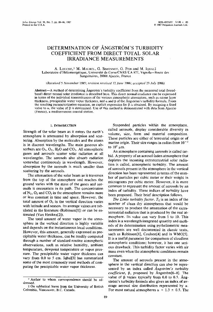
At the Laboratoire d'H61io6nerg~tique, Ajaccio, routine measurements of the normal irradiance using an automatic polar mounted Eppley model NIP pyrheliometer are being carried out since Oc- tober 1983. The present study includes data until September 1985. Tables of the average hourly flux summed at the end of each hour are available in a standard format. Also available are the daily traces of the normal irradiance. A typical example of such a trace is shown in Fig. 1. Deviations from a circular profile are during the moments when visible clouds are in line of sight from the observer to the sun. From these traces, all hours when the clouds did not intervene were identified. This yielded values of In from which values of 13 were computed; a total of 1175 data points.

(11) It is necessary to add here that when the sky is covered by a thin cloud throughout a day, the trace of normal flux will also have a circularform. There- fore, a visual inspection of the sky is useful to en- sure that the direct beam is uninterrupted by the clouds at the moment of observation. This is a pro- cedure followed when turbidity is measured by the spectral radiometers.

Due to the lack of local data on ozone, the av- erage values of the ozone layer thickness as given in Robinson[l] were used. For the latitude of Ajac- cio, average ozone layer thickness varies from 0.27 to 0.34 cm. It is known that attenuation by ozone is very small. Therefore, lack of exact data has only a minimal effect on the calculation of [3.

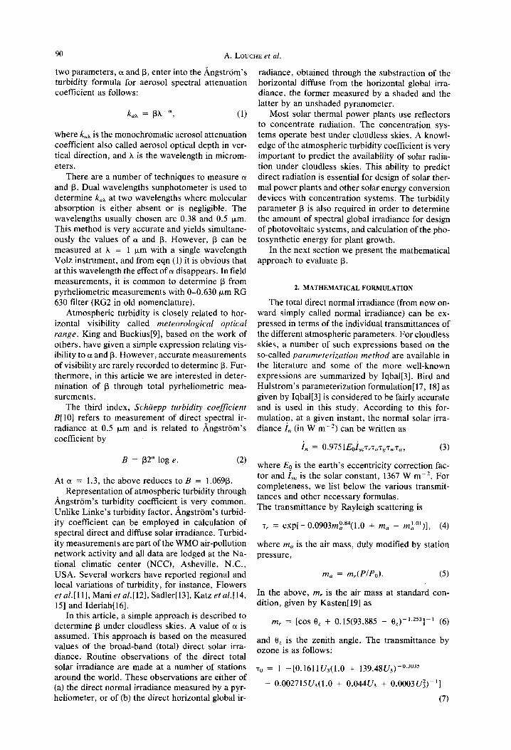
The relative humidity and ambient temperature data were obtained from the local office of meteo- rology. These data were used to calculate precip- itable water thickness from eqn (12). The values of

(14) w ranged from 0.5 cm in winter to 5 cm in summer. At these levels of the atmospheric water vapor, slight inaccuracies in the calculation of w are not

(15) important. This is demonstrated through Fig. 2. Slight variations in w when w is very low has a pro-

(16) nounced effect o n 1~ n compared to when w is high. (17) Furthermore, this effect remains independent of the

zenith angle. The station pressure was necessary to compute correct values of the air mass. This too

(18) was obtained from the local office of meteorology. The relative humidity and ambient temperature

data were taken at the synoptic hours, at every three hours of the standard time beginning mid- night. On the other hand, the radiation data were taken at the true solar time. Therefore, the relative humidity and temperature data had to be interpo- lated to correspond to the true solar time. As shown above, any error in the calculation of w through a linear interpolation will have a minimal effect, be- cause values of w were mostly quite high.

In the foregoing we have outlined the procedure

92

1 0 0 0 ~ ' 3=

. . . ~

800 - U,.I (3

z I o < 600 ¢_.

. J <

=E 4 0 0

0 Z

I- (3 ¢u 200 m C~

A. LOUCHE et al.

I ' ' I ' ' I ' ' I i , I J ' I ' ' ! '

Ajacc io

(41°55'N ; 8 ° 3 3 ' E )

~'~ 11 JULY 1985

0 3 6 9 NOON 15 18

TRUE S O L A R TIME

Fig. 1. The diurnal variation of direct normal irradiance.

21 24

I

E 3=

1000

03 =0.35 c¢ =1.3 8 = 0 . 2 2

900 ~

t U

z < a < Ix

-~ 8 0 0

. J <

0 z

I.- 700 (3 U.I n,,

6 O 0 0

ZENITH ANGLE 0 °

S

I t I , I , I 1 2 3 4

3 0 °

6 o o

P R E C I P I T A B L E WATER w cm i

Fig. 2. Direct normal irradiance as a funct ion o f precipitable water and zeni th angle.

Determination of ,~ngstrrm's turbidity coefficient

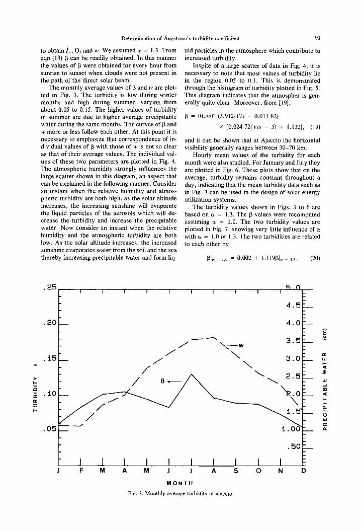
to obtain ~/,, O3 and w. We assumed a = 1.3. From eqn (13) [3 can be readily obtained. In this manner the values of [3 were obtained for every hour from sunrise to sunset when clouds were not present in the path of the direct solar beam.

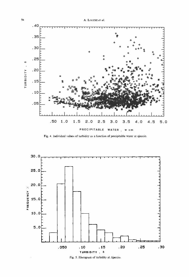
The monthly average values of [3 and w are plot- ted in Fig. 3. The turbidity is low during winter months and high during summer, varying from about 0.05 to 0.15. The higher values of turbidity in summer are due to higher average precipitable water during the same months. The curves of [3 and w more or less follow each other. At this point it is necessary to emphasize that correspondence of in- dividual values of [3 with those of w is not so clear as that of their average values. The individual val- ues of these two parameters are plotted in Fig. 4. The atmospheric humidity strongly influences the large scatter shown in this diagram, an aspect that can be explained in the following manner. Consider an instant when the relative humidity and atmos- pheric turbidity are both high, as the solar altitude increases, the increasing sunshine will evaporate the liquid particles of the aerosols which will de- crease the turbidity and increase the precipitable water. Now consider an instant when the relative humidity and the atmospheric turbidity are both low. As the solar altitude increases, the increased sunshine evaporates water from the soil and the sea thereby increasing precipitable water and form liq-

93

uid particles in the atmosphere which contribute to increased turbidity.

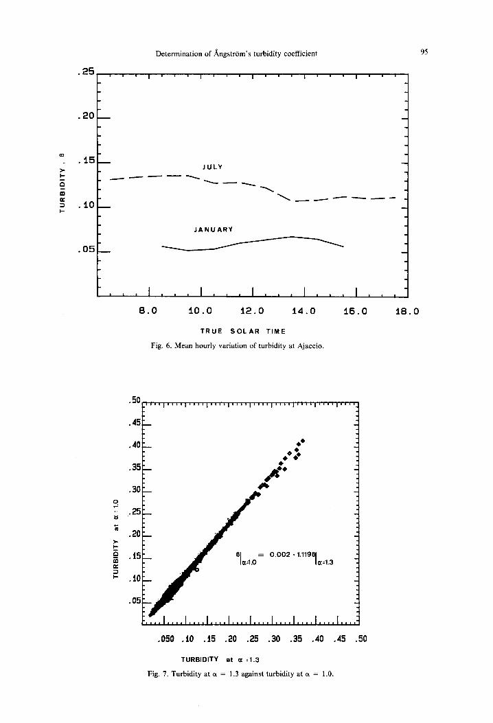
Inspite of a large scatter of data in Fig. 4, it is necessary to note that most values of turbidity lie in the region 0.05 to 0.1. This is demonstrated through the histogram of turbidity plotted in Fig. 5. This diagram indicates that the atmospher is gen- erally quite clear. Moreover, from [19],

[3 = (0.55) ~ ( 3 . 9 1 2 / V i s - 0.011 62)

x [0.024 7 2 ( V i s - 5) + 1.132], (19)

and it can be shown that at Ajaccio the horizontal visibility generally ranges between 30-70 km.

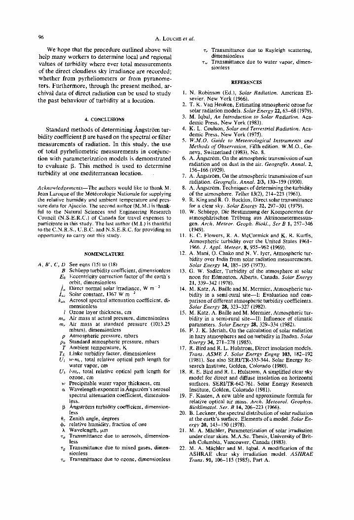
Hourly mean values of the turbidity for each month were also studied. For January and July they are plotted in Fig. 6. These plots show that on the average, turbidity remains constant throughout a day, indicating that the mean turbidity data such as in Fig. 3 can be used in the design of solar energy utilization systems.

The turbidity values shown in Figs. 3 to 6 are based on a = 1.3. The 13 values were recomputed assuming a = 1.0. The two turbidity values are plotted in Fig. 7, showing very little influence of a with c~ = 1.0 or 1.3. The two turbidities are related to each other by

[31~, = ,.o = 0.002 + 1.11913 K, Ls. (20)

• 2 5

• 2 0

. 1 5 / \

/ /

. i O

. 0 5

I I I I I I I I

>- l - a

IX

I-

I I I I I I I I F M A M J J A S

M O N T H

Fig . 3. M o n t h l y a v e r a g e t u r b i d i t y a t a j a c c i o .

\

I I

4.5

4.0

3.5

3.0

2.5

\

1 . 0 C

. 5 0

i I i 0 N D

¢ J v

t~ Ill I--

Lid ..I

I-"

e, m

O LU h- a .

94 A. LOUCHE et al.

I--

E

P

• 4 0

• 3 5

. 3 0

• 2 5

• 2 0

. 1 5

. I 0

. 0 5

' ' ' ' I ' ' ' ' I ' ' ' ' I ' ' ' ' I ' ' ' ' I ' ' ' ' I ' ' ' ' I ' ' ' ' I ' ' ' ' I ' ' '

@

@ @ @

¢L ~ U @ ,(~

. . • @ • I I B .m<~ ** 11

. 5 0 1 . 0 1 . 5 2 . 0 2 . 5 3 . 0 3 . 5 4 . 0 4 . 5

P R E C I P I T A B L E W A T E R w c m

Fig. 4. Individual values of turbidity as a function of precipitable water at ajaccio.

5 . 0

3 0 . 0 i i i I ' ' ' l ' ' ' ' l ' ' ' ' l ' ' ' ' l ' ' ' '

2 5 . 0 _ _

2 0 . O _ _

>- U Z " ' 1 5 . 0 3 0 uJ

i i

I 0 . 0

5 . O m

E • 0 5 0 . 1 0 . t 5 . 2 0 . 2 5

T U R B I D I T Y , 13

Fig. 5. Histogram of turbidity at Ajaccio,

. 3 0

.25

• 20

• 15 > -

I - -

o m I Z

= . iO

. 0 5

Determination of Angs t r fm ' s turbidity coefficient

' ' ' I ' ' ' I • ' ' I ' ' ' I ' ' ' I ' ' '

J U L Y

~ _ _ . . . . _ . _ _ _ _ ~ -

J A N U A R Y

, , , I . , , I . , . I , . , I , , , I , , ,

8 . 0 t 0 . 0 1 2 . 0 1 4 . 0 1 6 . 0 1 8 . 0

T R U E S O L A R T I M E

Fig. 6. Mean hourly variation of turbidity at Ajaccio.

95

.5O , , , i , , , . i , , , , i , , J , l , , . , i , , . . i , , , , l , . , . i , , , , i . . , .

.45 B

.40 _ *** .%*

.35 _ ~ Z +

.3o_ . ~ i

k / 1 ~ . 2 5

.20

. t 5 0 . 0 0 2 - 1.1198

~ . i o ~ . 0 5

.050 .t0 .15 .20 .25 .30 .35 .40 .45 .50

TURBIDITY at oc =1.3

Fig. 7. Turbidity at et = 1.3 against turbidity at et = 1.0.

96 A. LOUCHE et al.

We hope tha t the p r o c e d u r e out l ined a b o v e will he lp m a n y worke r s to de t e rmine local and regional va lues of turbidi ty whe re eve r total m e a s u r e m e n t s of the d i rec t c loudless sky i r rad iance are r ecorded ; w h e t h e r f rom pyrhe l iome te r s or f rom p y r a n o m e - ters. F u r t h e r m o r e , t h rough the p r e s en t m e t hod , ar- ch iva l da ta of d i rec t rad ia t ion can be used to s tudy the pa s t b e h a v i o u r of turbidi ty at a locat ion.

4. CONCLUSIONS

S t a n d a r d m e t h o d s of de t e rmin ing ~ n g s t r 6 m tur- b id i ty coeff ic ient 13 are based on the spect ra l or f i l ter m e a s u r e m e n t s of radia t ion. In this s tudy, the use o f to ta l py rhe l iomet r i c m e a s u r e m e n t s in con junc- t ion wi th p a r a m e t e r i z a t i o n mode ls is d e m o n s t r a t e d to eva lua te 13. This m e t h o d is used to de t e rmine tu rb id i ty at one m e d i t e r r a n e a n locat ion.

Acknowledgements--The authors would like to thank M. Jean Laroque of the M6t6orologie Nationale for supplying the relative humidity and ambient temperature and pres- sure data for Ajaccio. The second author (M.M.) is thank- ful to the Natural Sciences and Engineering Research Council (N.S.E.R.C.) of Canada for travel expenses to participate in this study. The last author (M.I.) is thankful to the C.N.R.S., U.B.C. and N.S.E.R.C. for providing an opportunity to carry out this study.

A , B ' , C , D B

Eo

L Isc kax

l ma

mr

NOMENCLATURE

See eqns (15) to (18) Schfiepp turbidity coefficient, dimensionless Eccentricity correction factor of the earth's orbit, dimensionless Direct normal solar irradiance, W m -2 Solar constant, 1367 W m -2 Aerosol spectral attenuation coefficient, di- mensionless Ozone layer thickness, cm Air mass at actual pressure, dimensionless Air mass at standard pressure (1013.25 mbars), dimensionless

p Atmospheric pressure, mbars P0 Standard atmospheric pressure, mbars T Ambient temperature, K

TL Linke turbidity factor, dimensionless UI w.mr, total relative optical path length for

water vapor, cm U3 l'mr, total relative optical path length for

ozone, cm w Precipitable water vapor thickness, cm a Wavelength exponent in/ ingstr6m's aerosol

spectral attenuation coefficient, dimension- less. Angstr6ms turbidity coefficient, dimension- less

0z Zenith angle, degrees +~ relative humidity, fraction of one h Wavelength, i~m

"r~ Transmittance due to aerosols, dimension- less

% Transmittance due to mixed gases, dimen- sionless

ro Transmittance due to ozone, dimensionless

• r Transmittance due to Rayleigh scattering, dimensionless

T,, Transmittance due to water vapor, dimen- sionless

REFERENCES

1. N. Robinson (Ed.), Solar Radiation. American El- sevier, New York (1966).

2. T. K. Van Heuken, Estimating atmospheric ozone for solar radiation models. Solar Energy 22, 63-68 (1979).

3. M. Iqbal, An Introduction to Solar Radiation. Aca- demic Press, New York (1983).

4. K. L. Coulson, Solar and Terrestrial Radiation. Aca- demic Press, New York (1975).

5. W.M.O. Guide to Meteorological Instruments and Methods of Observation, Fifth edition. W.M.O., Ge- neva, Switzerland (1983), No. 8.

6. A. ,~.ngstr6m, On the atmospheric transmission of sun radiation and on dust in the air. Geografis, Annal. 2, 156-166 (1929).

7. A. ,~ngstr6m, On the atmospheric transmission of sun radiation. Geografis. Annal. 2/3, 130-159 (1930).

8. A./~ngstr6m, Techniques of determining the turbidity of the atmosphere. Tellus 13(2), 214-223 (1961).

9. R. King and R. O. Buckius, Direct solar transmittance for a clear sky. Solar Energy 22, 297-301 (1979).

10. W. Sch0epp, Die Bestimmung der Komponenten der atmosph/irischen Triibung aus Aktinometermessun- gen. Arch. Meteor. Geoph. Biokl., Ser B 1, 257-346 (1949).

11. E. C. Flowers, R. A. McCormick and K. R. Kurfis, Atmospheric turbidity over the United States 1961- 1966. J. Appl. Meteor. 8, 955-962 (1969).

12. A. Mani, O. Chako and N. V. Iyer, Atmospheric tur- bidity over India from solar radiation measurements. Solar Energy 14, 185-195 (1973).

13. G. W. Sadler, Turbidity of the atmosphere at solar noon for Edmonton, Alberta, Canada. Solar Energy 21, 339-342 (1978).

14. M. Katz, A. Baille and M. Mermier, Atmospheric tur- bidity in a semi-rural si te--I: Evaluation and com- parison of different atmospheric turbidity coefficients. Solar Energy 28, 323-327 (1982).

15. M. Katz, A. Baille and M. Mermier, Atmospheric tur- bidity in a semi-rural site--II: Influence of climatic parameters. Solar Energy 28, 329-334 (1982).

16. F. J. K. Ideriah, On the calculation of solar radiation in hazy atmospheres and on turbidity in Ibadan. Solar Energy 34, 271-278 (1985).

17. R. Bird and R. L. Hulstrom, Direct insolation models. Trans. ASME J. Solar Energy Engng 103, 182-192 (1981). See also SERI/TR-335-344. Solar Energy Re- search Institute, Golden, Colorado (1980).

18. R. E. Bird and R. L. Hulstrom, A simplified clear sky model for direct and diffuse insolation on horizontal surfaces. SERIfrR-642-761. Solar Energy Research Institute, Golden, Colorado (1981).

19. F. Kasten, A new table and approximate formula for relative optical air mass. Arch. Meteorol. Geophys. Bioklimatol. Ser. B 14, 206-223 (1966).

20. B. Leckner, the spectral distribution of solar radiation at the earth's surface. Elements of a model. Solar En- ergy 20, 143-150 (1978).

21. M. A. Mfichler, Parameterization of solar irradiation under clear skies. M.A.Sc. Thesis, University of Brit- ish Columbia, Vancouver, Canada (1983).

22. M. A. M/ichler and M. Iqbal. A modification of the ASHRAE clear sky irradiation model. ASHRAE Trans. 91, 106-115 (1985), Part A.