University of South CarolinaScholar Commons

Theses and Dissertations

2017

Determination and Validation of High-PressureEquilibrium Adsorption Isotherms via aVolumetric SystemHind Jihad Kadhim ShabbaniUniversity of South Carolina

Follow this and additional works at: https://scholarcommons.sc.edu/etd

Part of the Chemical Engineering Commons

This Open Access Thesis is brought to you by Scholar Commons. It has been accepted for inclusion in Theses and Dissertations by an authorizedadministrator of Scholar Commons. For more information, please contact dillarda@mailbox.sc.edu.

Recommended CitationShabbani, H. J.(2017). Determination and Validation of High-Pressure Equilibrium Adsorption Isotherms via a Volumetric System.(Master's thesis). Retrieved from https://scholarcommons.sc.edu/etd/4310

DETERMINATION AND VALIDATION OF HIGH-PRESSURE EQUILIBRIUM

ADSORPTION ISOTHERMS VIA A VOLUMETRIC SYSTEM

By

Hind Jihad Kadhim Shabbani

Bachelor of Science

Al-Qadisiya University, 2013

Submitted in Partial Fulfilment of the Requirements

For the Degree of Master of Science in

Chemical Engineering

College of Engineering and Computing

University of South Carolina

2017

Accepted by:

James A. Ritter, Director of Thesis

Armin Ebner, Reader

Jamil Khan, Reader

John Weidner, Reader

Cheryl L Addy, Vice Provost and Dean of the Graduate School

ii

© Copyright by Hind Jihad Kadhim Shabbani, 2017

All Rights Reserved.

iii

ACKNOWLEDGEMENTS

“Let gratitude be the pillow upon which you kneel to say your nightly prayer

- Dr Maya Angelou

First and foremost I acknowledge first the Higher Committee of Education in Iraq

(HCED) that gave me the chance to pursue my degree and offer me sponsorship

throughout the way. Secondly, I would like to express my gratitude to Dr James Ritter for

accepting me as one of his students and giving me the opportunity to work with him.

Special acknowledgement to Dr Ebner Armin who took upon himself to be a true

guidance and amazing teacher, his patience and understanding will always be

acknowledged. I would also like to acknowledge the efforts of Dr Nicholson Marjorie

who gave time and effort in helping me in my research.

Thanks to my two amazing children who gave me hope and happiness through the

hardest times. A full-hearted acknowledgement to the two men who believed in me since

the beginning, my husband and my father. Thank you for your faith and encouragement,

it helped me to be a better student and a better person. My mother, sisters and brothers I

appreciate all your prayers and support.

Finally, to all who ever supported me with a kind word or simply by a smile, I’d like to

express my gratitude to you for being a part of this journey.

iv

ABSTRACT

Adsorption equilibrium isotherms for N2, CO2, and CH4 on zeolite 13X were

investigated at three different temperatures (25.5, 50.5 and 75.5 ̊ C) and a pressure range

of (0-6.89475) MPa for CH4 and N2 and in the range of (0-4.82633) MPa for CO2 using

built in volumetric apparatus. The results were validated using with a volumetric system

(ASAP) at the same temperatures and a pressure up to (160-110) KPa respectively. The

experimental results were correlated using three process Langmuir (TPLM). The

correlated isotherms were then used to calculate the isosteric heat of adsorption for the

three gases on 13X. The resulting data have been used to validate the measurements of

these systems and are available in the literature for comparison of zeolite 13X isotherms

with newly developed adsorbents.

v

TABLE OF CONTENTS

ACKNOWLEDGEMENTS ........................................................................................................ iii

ABSTRACT .......................................................................................................................... iv

LIST OF TABLES .................................................................................................................. vi

LIST OF FIGURES ............................................................................................................... viii

CHAPTER 1 INTRODUCTION ....................................................................................................1

CHAPTER 2 EXPERIMENTAL ...................................................................................................6

Materials ........................................................................................................................6

Experimental setup.........................................................................................................6

Sample chamber .............................................................................................................8

Volume determination of system elements ....................................................................9

Sample regeneration.....................................................................................................11

Isotherm determination ................................................................................................12

Isotherms model .......................................................................................................... 15

The Isosteric heat of adsorption ...................................................................................16

CHAPTER 3 RESULTS AND DISCUSSION .................................................................................18

Conclusion ...................................................................................................................20

REFERENCES ........................................................................................................................47

vi

LIST OF TABLES

Table 1. 1: composition values for Gas produced from Antrim Shale wells, USA (mol. %)

[21] ..................................................................................................................................... 4

Table 1. 2: Natural gas geothermal characteristic compassion from Jiaoshilba, China,

shale gas field [22]. ............................................................................................................. 4

Table 1. 3: Molecular composition of Chestnut park and Clarington seep gases, USA,

(vol. %) [23]. ....................................................................................................................... 4

Table 1. 4: Longmaxi shale gas main component molecular composition (%) in southern

Sichuan Basin, China [24]. ................................................................................................. 5

Table 3. 1: experimental values of the system different volumes ..................................... 27

Table 3. 2: Relevant thermodynamic properties of adsorbates [26] ................................. 27

Table 3. 3: Relevant physical properties of adsorbates [28] ............................................. 27

Table 3. 4: Adsorption Equilibrium Isotherm Data of Nitrogen on 13X at 25.5, 50.5, and

75.5 oC measured by volumetric setup ............................................................................. 28

Table 3. 5: Adsorption Equilibrium Isotherm Data of carbon dioxide on 13X at 25.5,

50.5, and 75.5 oC measured by volumetric setup ............................................................. 29

Table 3. 6: Adsorption Equilibrium Isotherm Data of methane on 13X at 25.5, 50.5, and

75.5 oC measured by volumetric setup ............................................................................. 30

Table 3. 7: Adsorption Equilibrium Isotherm Data of Nitrogen on zeolite 13X at 25, 50,

and 75 oC measured by ASAP2010.................................................................................. 31

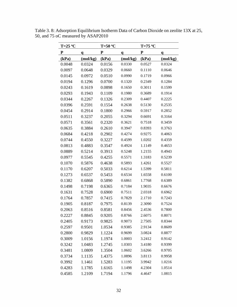
Table 3. 8: Adsorption Equilibrium Isotherm Data of Carbon Dioxide on zeolite 13X at

25, 50, and 75 oC measured by ASAP2010...................................................................... 32

Table 3. 9: Adsorption Equilibrium Isotherm Data of Methane on zeolite 13X at 25, 50,

and 75 oC measured by ASAP2010.................................................................................. 35

Table 3. 10: Fitting parameters of the Three Process Langmuir model for 13X .............. 36

vii

Table 3. 11: Adsorption Equilibrium Isotherm Data of nitrogen on zeolite 13X at 25, 50

◦C measured by Park [18]. ................................................................................................ 36

Table 3. 12: Adsorption Equilibrium Isotherm Data of Carbon dioxide on zeolite 13X at

25, 50 ◦C measured by Park [18]. ..................................................................................... 38

Table 3. 13: Adsorption Equilibrium Isotherm Data of Methane on zeolite 13X at 25, 50

◦C measured by Park [18]. ................................................................................................ 39

Table 3. 14: Adsorption Equilibrium Isotherm Data of nitrogen on zeolite 13X at 25, 50

◦C measured by Simone Cavenati [19]. ............................................................................ 41

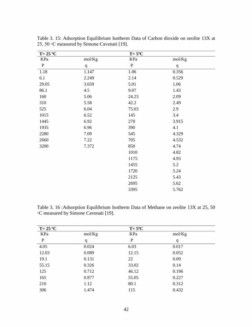
Table 3. 15: Adsorption Equilibrium Isotherm Data of Carbon dioxide on zeolite 13X at

25, 50 ◦C measured by Simone Cavenati [19]. ................................................................. 42

Table 3. 16 :Adsorption Equilibrium Isotherm Data of Methane on zeolite 13X at 25, 50

◦C measured by Simone Cavenati [19]. ............................................................................ 42

Table 3. 17: Henry’s constant for the volumetric system compared to the ones in the

literature. ........................................................................................................................... 43

viii

LIST OF FIGURES

Figure 2. 1: detailed schematic for the volumetric setup. ................................................... 8

Figure 2. 2: a) Schematic of sample chamber and b) actual components of the sample

chamber. .............................................................................................................................. 9

Figure 3. 1: Adsorption equilibrium isotherms of Nitrogen fitted with TPL model at three

different temperatures on 13X in rectangular coordinates ................................................ 22

Figure 3. 2: Adsorption equilibrium isotherms of Nitrogen fitted with TPL model at three

different temperatures on 13X in logarithmic scale .......................................................... 22

Figure 3. 3: Adsorption equilibrium isotherms of carbon dioxide fitted with TPL model at

three different temperatures on 13X in rectangular coordinates ....................................... 23

Figure 3. 4: Adsorption equilibrium isotherms of carbon dioxide fitted with TPL model at

three different temperatures on 13X in logarithmic scale ................................................. 23

Figure 3. 5: Adsorption equilibrium isotherms of methane fitted with TPL model at three

different temperatures on 13X in rectangular coordinates ................................................ 24

Figure 3. 6: Adsorption equilibrium isotherms of methane fitted with TPL model at three

different temperatures on 13X in logarithmic scale .......................................................... 24

Figure 3. 7: Isosteric heat of adsorption for N2 on 13X with respect to loadings for three

different temperatures (Isosteric heat of adsorption equation derived from TPL model) 25

Figure 3. 8: Isosteric heat of adsorption for CO2 on 13X with respect to loadings for three

different temperatures (Isosteric heat of adsorption equation derived from TPL model) 25

Figure 3. 9: Isosteric heat of adsorption for CH4 on 13X with respect to loadings for three

different temperatures (Isosteric heat of adsorption equation derived from TPL model) 26

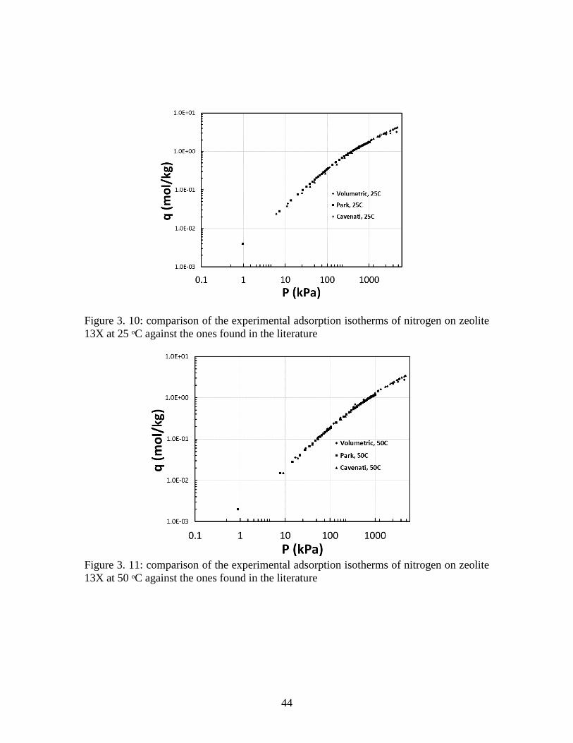
Figure 3. 10: comparison of the experimental adsorption isotherms of nitrogen on zeolite

13X at 25 ᵒC against the ones found in the literature ........................................................ 44

Figure 3. 11: comparison of the experimental adsorption isotherms of nitrogen on zeolite

13X at 50 ᵒC against the ones found in the literature ........................................................ 44

ix

Figure 3. 12: comparison of the experimental adsorption isotherms of carbon dioxide on

zeolite 13X at 25 ᵒC against the ones found in the literature ............................................ 45

Figure 3. 13: comparison of the experimental adsorption isotherms of carbon dioxide on

zeolite 13X at 50 ᵒC against the ones found in the literature ............................................ 45

Figure 3. 14: comparison of the experimental adsorption isotherms of methane on zeolite

13X at 25ᵒC against the ones found in the literature ......................................................... 46

Figure 3. 15: comparison of the experimental adsorption isotherms of methane on zeolite

13X at 50 ᵒC against the ones found in the ....................................................................... 46

1

CHAPTER 1

INTRODUCTION

The slow but steady decline, despite continuous drilling of natural gas that is

considered both cheap and clean source of energy, have put the unconventional sources of

natural gas especially shale gas in center-stage. Shale gas and the unconventional sources

of natural gas have risen in recent years due to the economic feasibility of extracting these

unconventional sources which helped in transforming the energy sector in the United

States. Shale gas has been produced on a large scale, almost half the United States supply

of natural gas and is expected to make up 14% of the world energy by 2035 according to

the international energy agency (IEA). Shale gas which is usually found in low porosity

organic shale rocks is being produced by performing hydraulic fracturing and horizontal

drilling. Shale gas is mainly composed of methane and small fractions of C2, C3, CO2, N2,

and a trace amount of other material such as H2S (refer to Table 1.1, 1.2, 1.3 and 1.4).

Fracking fluid is pumped into the well under high pressures which could be ranging from

3.44 MPa up to 85 MPa [1] [2] [3] [4] [5] [6]. After the fracking process is finished, the

produced shale gas needs to be sequestered and purified for future use.

High-pressure adsorption attracts research in recent years due to the rise in the

production of natural gas that results from unconventional sources such as shale gas.

Adsorption isotherms can be measured experimentally using different techniques, but

2

usually, the most common methods are volumetric and gravimetric. Volumetric method is

usually preferable in the laboratory due to its simplicity and low cost [7].

The separation and purification of a gas stream based on a selective adsorption on

a solid adsorbent material to produce a gas stream enriched with the less likely adsorbed

gas have been used widely in industrial applications [8][9][10]. Adsorption processes such

as pressure swing adsorption (PSA) and temperature swing adsorption (TSA) have gained

an increased interest in the past years in purification and separation processes. The

increased used of these processes is mainly due to low energy required and low capital cost

[10]. The most important criteria for choosing an adsorbent for PSA is its adsorption

working capacity and selectivity at the conditions required. The most common adsorbents

are activated carbon and zeolite due to their large internal surface and complicated pore

system [11]. Activated carbon is the most prevalent adsorbent used in separation and

purification processes as consequence of its low cost and large surface area [12] [13].

Zeolite, on the other hand, is a crystalline porous aluminosilicate that is being used in the

separation processes greatly due to its well-defined structure, surface basicity, the electric

field caused by exchangeable cations that are present in its framework, 3D pores and well-

defined diameter [8] [14] [15]. It was found that zeolite 13X (NaX) is one of the best types

of zeolite in the adsorption process due to its stability, higher capacity and rapid mass

transfer [15].

The development of PSA process design and simulation requires the knowledge of

the adsorption equilibrium data such as adsorption isotherms and the isosteric heat of

adsorption on a broad range of temperatures and pressures [12] [16]. Adsorption isotherms

represent the amount adsorbed (moles of adsorbate/gm of adsorbent) versus pressure at

3

constant temperature. The availability of isotherms data will help determine the critical

dimensions and operation time for adsorption processes design. The adsorption isotherms

could be of different shapes reflecting the type of the adsorbate-adsorbent interaction [17]

[8]. High-pressure adsorption isotherms are of particular importance considering that it

could be used for the separation, purification, and storage of the shale gas.

There have been many studies in the literature on high-pressure adsorption. The

adsorption equilibria of CO2, CO, N2, CH4, Ar and H2 were measured on pelletized 13X

up to 1 MPa by Park et al [18] using volumetric technique for the temperatures (20, 35 and

50) ̊C, the isosteric heat of adsorption was also measured from collating experimental

results using Langmuir and sips model. High-pressure adsorption isotherms on zeolite 13X

were also reported in the literature. The adsorption equilibria of CH4, N2 and CO2, were

measured on 13X using the gravimetric technique at a three different temperatures (25, 35

and 50) ̊C and in a pressure range of (0-5) MPa by Cavenati et al. [19]. Their results showed

that the adsorption capacity of CO2 on 13X is much higher than the other gases and that

13X could be used for natural gas purification or carbon dioxide capture [19]. High

pressure adsorption of CO2 on 13X using PSA was also investigated by Takamura et al.

[20].

In this work, the pure adsorption isotherms of different gases (CH4, N2 and CO2)

were measured using the volumetric technique on and zeolite 13X at three temperatures

(25.5, 50.5 and 75.5) ̊C and in the pressure range of (0-6.895) MPa. The results obtained

on 13X were validated by comparison to the ones obtained by ASAP volumetric systems.

The heat of adsorption was also calculated for the three gases on13X zeolite using three

process Langmuir model (TPLM) These results can be considered as a reference data for

4

future researches, help in the evaluation of the adsorption capacity of recently developed

adsorbents and they could also help with the design of adsorption processes that contain

the studied gases under the studied conditions.

Tables (1.1, 1.2, 1.3 and 1.4) show the different possible composition for shale gas

for different areas and different sources.

Table 1. 1: composition values for Gas produced from Antrim Shale wells, USA (mol. %)

[21].

Well, state C1 C2 C3 CO2 N2

Northern

margin

Michigan

77.34-96.75 0-3.96 0-0.92 0.01-5.75 0.28-14.33

Western

margin,

Michigan

60.37-92.48 0.06-6.64 0.07-2.63 3.42-7.47 0.10-28.84

Central Basin ,

Michigan

57.80-81.16 4.94-11.92 1.87-4.90 0.04-0.17 0.51-36.19

Southern

margin,

Indiana

27.18-85.37 3.45-4.29 0.4-1 2.97-8.92 0.72-64.27

Southern

margin, Ohio

62.24-73.17 0.07-4.76 0.25 0.17-4.46 28.00

Southern

margin,

Michigan

45.46 5.78 1.8 2.89 43.52

Eastern margin

, Michigan

84.62 6.13 1.65 1.22 6.03

Table 1. 2: Natural gas geothermal characteristic compassion from Jiaoshilba, China, shale

gas field [22].

C1 C2 C3 CO2 N2 95.52-98.95 0.32-0.73 0.01-0.05 0.02-1.07 0.32-2.95

Table 1. 3: Molecular composition of Chestnut park and Clarington seep gases, USA, (vol.

%) [23].

sample C1 C2 C3 iC4 nC4 iC5 C6+ CO2 N2 He H2 C1

Chestnut 59.75 23.48 11.69 0.810 2.059 0.214 0.120 1.553 0.244 0.005 0.058 59.75

Clarington 87.75 8.50 2.15 0.277 0.400 0.090 0.056 0.07 4.91 0.075 0.262 87.75

5

Table 1. 4: Longmaxi shale gas main component molecular composition (%) in southern

Sichuan Basin, China [24].

C1 C2 C3 CO2 N2 97.64-99.59 0.23-0.68 0-0.03 0.01-1.148 0.01-2.95

6

CHAPTER 2

EXPERIMENTAL

Materials

The zeolite 13X was supplied by Grace Davison (grade 544, 8x12 mesh size).

Helium, Nitrogen and methane were provided from PRAXAIR with a purity of 99.999,

99.999 and 99.97% respectively, while carbon dioxide was provided from Airgas with a

purity of 99.99%

Experimental Setup

Figure 2.1 shows a schematic of the volumetric setup used in this work. It consisted

of two volumetric cells: an antechamber of known volume (9) and a sample chamber (12)

separated by both a needle (10) and a ball valve (11). The needle valve is used to regulate

the flow between the two cells and the ball valve to isolate the cells from each other during

isotherm determination. Additional needle and ball valve pairs are also placed upstream

the antechamber (5 and 8) and downstream the sample chamber (13 and 14). The first pair

(i.e., valves 5 and 8) is used to regulate the flow into the antechamber and allow or not gas

into the antechamber during isotherm determination. The second pair (i.e., valves 13 and

14) are used to regulate and allow the flow leaving the sample chamber during regeneration

of the sample via gas purge, which is a step that is explained in more detailed later. The

pressure within these cells is measured by using three MKS pressure transducers (19, 20

and 21) that read up to 1000, 250 and 30 Psia, respectively. Two ball valves (17 and 18)

7

were used to protect the lower pressure transducers 20 and 21, respectively, when operating

at pressures that were higher than the maximum recommended values for each one of them.

A 15-micron filter (16) is used to protect the transducer from sample dust that may be

coming from the sample chamber. The temperature of the sample in the sample chamber

is measured by a K type thermocouple (15). A Pfeiffer (TSU 071 E) vacuum pump (7)

able to achieve a vacuum up to 5.4x10-5 mbar is attached upstream needle valve 6 is used

for both sample regeneration (also as explained later). A three-way valve (4) is connected

between the system and the vacuum pump with the common exit attached to the system so

that the system is depressurized via venting of via evacuation through the pump. Feed

gassed are admitted into the system through ball valve 1. A three-way valve (2) with the

common exit connected toward the feed is used to vent the lines prior to any run. The two

volumetric cells, valves 8, 10, 11 13, and 14, and the filter 16 are all placed within a

THERMOTRON temperature chamber to keep the temperature of the system controlled at

a constant valve during the isotherm determination. All tubing lines used within the

chamber were 1/16th inch OD. The figure does not show band heaters and glass wool

insulation that are temporarily put around the sample chamber for regeneration. These band

heater and insulation are removed during isotherm determination or any run that is carried

out at lower temperatures.

8

Figure 2. 1: detailed schematic for the volumetric setup.

Sample Chamber

The sample chamber is described in figure (2.2) with detailed schematic (a) and

picture of the actual cell and parts involved (b). The chamber consisted of an upper flange

(11) containing a k-type thermocouple (2) previously described, a lower flange weld to the

sample holding bed (6), a cylindrical sample holder (7) and a mesh holder (4) both made

of aluminum, the mesh (10) is used to keep samples that consist of fine powders confined

within the chamber cell, and a copper gasket placed between the flanges to seal the chamber

cell from leaking (3). Depending on the sample holder, the sample chamber can contain up

to 20 g of sample (5). Eight bolts (1) are used to seal the system by bringing both flanges

against each other and squeezing the copper gasket. The tip of the thermocouple is placed

within the bulk of the sample as shown. The gas access (8) and exit (9) to and from the

sample chamber is done through sample holding bed wall. The corresponding gas lines are

9

connected to the sample chamber via 1/16th vcr fittings. Within the sample chamber, the

gas moves upward and downward through the space between the sample holder and the

inner wall of the sample chamber before and after it reaches the sample, respectively.

Figure 2. 2: a) Schematic of sample chamber and b) actual components of the sample

chamber.

Volume Determination of System Elements

The volumes of the antechamber Vac, empty sample chamber Vs (i.e., without

sample, mesh, mesh holder and sample holders), sample and mesh holder together Vh, and

the skeletal volume of the sample Va are determined in different runs with helium and with

the aid of steel spheres of known volume Vsph. The following four runs are carried out. A

first run with the sample chamber being empty; a second run with the sample chamber

containing only the spheres of known value; a third run with the sample chamber

containing both sample and mesh holders and mesh but without the sample, and a fourth

run with the sample chamber containing both sample and mesh holders, mesh and a

regenerated sample. In all these runs the same following three steps are carried out. First,

the antechamber and sample chamber must be under complete vacuum. This is done by

b a

1

1

2

1 3

1 4

21

5

1

6

1

7

1

8

1

9

1

10

1

11

1

10

evacuating these chambers that were originally under helium by opening valves 8, 11, and

the three-way valve 4 connecting the both chambers to the vacuum pump. All other valves

remain closed. Then, valve 11 and the three-way valve 4 are closed and valves 1, 3, and 8

are opened (with three-way valve 2 connecting helium to the antechamber) to let helium in

to pressurize the antechamber from vacuum to a desired pressure, by closing valve 8 again.

The pressure within the antechamber is let equilibrate to an initial pressure Pi. Finally ball

valve 11 is opened to connect both antechamber and sample chamber. Thus, helium from

the antechamber is expanded into the sample chamber (12), which was originally under

vacuum. The pressure of the two connecter chambers is let to equilibrate to a final pressure

Pf.

The volumes of the antechamber and empty sample chamber are obtained from the

run with sample chamber being empty, for which the initial and final pressures are

𝑃𝑒𝑚𝑝𝑡𝑦𝑖 , 𝑎𝑛𝑑 𝑃𝑒𝑚𝑝𝑡𝑦

𝑓 , and the run with the sample chamber containing the spheres of known

volume 𝑉𝑠𝑝ℎ, for which the initial and final pressures are 𝑃𝑠𝑝ℎ𝑖 , 𝑎𝑛𝑑 𝑃𝑠𝑝ℎ

𝑓, according to the

expressions:

𝑉𝑎𝑐 = 𝑉𝑠𝑝ℎ ∙

(

1

𝑃𝑒𝑚𝑝𝑡𝑦𝑓

𝑃𝑒𝑚𝑝𝑡𝑦𝑖 −

𝑃𝑠𝑝ℎ𝑓

𝑃𝑠𝑝ℎ𝑖 )

(1)

𝑉𝑠 = 𝑉𝑎𝑐 ∙ (𝑃𝑒𝑚𝑝𝑡𝑦𝑓

𝑃𝑒𝑚𝑝𝑡𝑦𝑖 − 1) (2)

11

The volume used by the sample holder, mesh holder and mesh Vh is then obtained

from the pressures 𝑃ℎ𝑖 , 𝑎𝑛𝑑 𝑃ℎ

𝑓from the run with sample chamber containing the holders

and the mesh without the sample according to:

𝑉ℎ = 𝑉𝑠 − 𝑉𝑎𝑐 ∙ (𝑃ℎ𝑓

𝑃ℎ𝑖 − 1) (3)

Finally, the volume used by the regenerated sample is also obtained from the pressures

𝑃𝑠𝑖 , 𝑎𝑛𝑑 𝑃𝑠

𝑓from the run with sample chamber containing all sample, holders and mesh

according to:

𝑉𝑎 = 𝑉𝑠 − 𝑉ℎ − 𝑉𝑎𝑐 ∙ (𝑃𝑠𝑓

𝑃𝑠𝑖 − 1) (4)

Sample regeneration.

Two types of regeneration were carried out on the zeolite 13X sample depending

whether the sample was a new sample or whether the sample was already tested with one

gas and required analysis with a different gas. In the first case, the sample is purged through

with the helium at a flow of no more than 50 cc/min. This was done by having the three-

way valve 2 connecting helium with the antechamber, and then opening valves 1, 3, 8, 11

and 13 while having the rest of the valves closed. Then the sample chamber is brought up

to 100 oC and kept there for an hour before the temperature is raised again to 350 ºC to

leave the sample chamber at that temperature overnight. As previously indicated a band

heater and glass wool insulation was placed around sample chamber during regeneration.

Before cooling down, valves 3, and 13 are closed, the three-way valve 4 is adjusted to

connect the antechamber with the vacuum pump and the system is let fully evacuate. After

12

the system cools down, the band heater and glass insulation is removed and the

THERMOTRON chamber is set to the desired experimental temperature. In the case of

changing the working gas (i.e., adsorbate), the sample is purged through with the new

working gas at a flow of no more than 50 cc/min. This was done by having the three-way

valve 2 connecting the working gas with the antechamber, and then opening valves 1, 3, 8,

11 and 13 while having the rest of the valves closed. Then sample chamber is the brought

up only to 160 oC this time and kept there overnight. Again, a band heater and glass wool

insulation was placed around sample chamber during this time. This is done to remove any

traces of the previous working gas in the sample. After purging at 160 oC for an hour,

valves 3, and 13 are then closed, the three-way valve 4 is adjusted to connect the

antechamber with the vacuum pump and the system is let fully evacuate. Vacuum

regeneration at 160 oC is then continued overnight. After the system cools down, the band

heater and glass insulation is removed and the THERMOTRON chamber is set to the

desired experimental temperature.

Isotherm Determination

Isotherms of any of the three tested gasses (N2, CH4 and CO2) were obtained by

setting the temperature controller of the THERMOTRON temperature chamber set at the

desired temperature. The isotherm determination process was initialized by first having

both antechamber and sample chamber under vacuum, with all valves closed except for

valves 1 and 3 and the three-way valve 2 that was set to connect the working gas with the

line feeding the antechamber through valves 3 and 8 (which is closed). The sample chamber

which contains the sample holder, the mesh holder, the mesh and a sample of zeolite 13X

of mass ma that has been previously regenerated. Valve 8 is then opened and the

13

antechamber is let pressurized till the desired pressure is reached by closing valve 8 again.

The antechamber is let equilibrate and initial pressure of this step 𝑃1𝑖 is recorded and the

total moles of the working gas into the system is determined based on thee known volume

of the antechamber Vac and assuming a real gas equation of state for the working gas. Then

ball valve 11 is opened and the gas from the antechamber is expanded into the sample

chamber. The connected antechamber and sample chamber are to let to equilibrate for the

next 60 min to have the final pressure of the step 𝑃1𝑓 recorded. The latter piece information

will help evaluate the first point of the isotherm. Valve 11 is then closed and valve 8 is

reopened to start the second step by refilling the antechamber with the working gas to a

new desired pressure by closing again valve 8. The antechamber is let equilibrate and the

new initial pressure 𝑃2𝑖 of the second step is recorded and then used together with 𝑃1

𝑓 to

evaluate the new mass of working gas into the system. The valve 11 is reopened and the

system is again let to equilibrate for the next 60 min to get both the final pressure of step

two 𝑃2𝑓 to evaluate the second point of the isotherm. Valve 11 is closed and the process of

opening and closing valve 8 and opening and closing valve 11 repeated up to the desired

pressures within the limits of the higher most transducer (i.e, 1000 Psia). Numerically, a

point of the isotherm at step j, qj, in equilibrium at temperature T and final pressure Pjfthat

is determined when both antechamber and sample chamber are connected (valve 11 open

and valve 8 closed) is calculated from the following expressions:

𝑞𝑗(𝑃𝑗𝑓, 𝑇) =

𝑁𝑗𝑎

𝑚𝑎 (5)

Nja = Nj

T − Njg (6)

14

Njg=

Pjf

𝑅𝑇∙

𝑉𝑒𝑥

𝑍(Pjf,T)

(7)

NjT = Nj−1

T + ∆Nj (8)

∆Nj = Njac,i − Nj−1

𝑎𝑐,𝑓 (9)

Njac,i =

Pji

𝑅𝑇∙𝑉𝑎𝑐

𝑍(Pji,T)

(10)

Nj−1ac,f =

Pj−1f

𝑅𝑇∙

𝑉𝑎𝑐

𝑍(Pj−1f ,T)

(11)

With

NoT = 0 𝑎𝑛𝑑 𝑃𝑜 = 0 (12)

Where NjT, Nj

a𝑎𝑛𝑑Njg respectively correspond to the total moles of working gas

(both adsorbed and gas phase), the total moles of working gas in adsorbed state and the

total moles of working gas in gas state within the system that comprise the antechamber

and sample chamber; Pji and Pj

f respectively correspond to the equilibrium pressures of the

antechamber before and after the gas expansion into the sample chamber through valve 11

; Njac,i, Nj

ac,f are the moles of the antechamber before and after the gas expansion into the

sample chamber through valve 11, ∆Nj are the new moles of working gas into the system,

Vex corresponds to the excluded volume of the system, which is given by:

𝑉𝑒𝑥 = 𝑉𝑎𝑐 + 𝑉𝑠 − 𝑉ℎ − 𝑉𝑎 (13)

And Z (P, T) is the compressibility factor, which is calculated from Pitzer

Correlations [26]:

15

𝑍(𝑃, 𝑇) = 𝑍𝑜(𝑃, 𝑇) + 𝑤 ∗ 𝑍1(𝑃, 𝑇) (14)

𝑍𝑜(𝑃, 𝑇) = 𝐵𝑜 ∗ (𝑃𝑟

𝑇𝑟) (15)

𝑍1(𝑃, 𝑇) = 𝐵𝑜 ∗ (𝑃𝑟

𝑇𝑟) (16)

𝐵𝑜 = 0.083 −0.422

𝑇𝑟1.6 (17)

𝐵1 = 0.139 −0.172

𝑇𝑟4.2 (18)

𝑃𝑟 =𝑃

𝑃𝑐 (19)

𝑇𝑟 =𝑇

𝑇𝑐 (20)

where Pr and Tr is the reduced pressure and temperature, respectably and Tc, Pc and w are

the critical temperature, the critical pressure, and acentric factor of the working gas

respectively. Refer to table 3.2.

Isotherm Models

Adsorption equilibrium data were correlated using two models for pure gasses to

be used in getting the isosteric heat of adsorption Qst of the gas as a function of loading.

These two models are the Three Process Langmuir and the Toth equation. Isotherm data

obtained elsewhere at lower pressures using an ASAP 2010 volummetric system [28] for

the same gasses on the same 13X zeolite from Grace Davison was included in the fitting

of these models. All the data from a single gas at all three different temperatures obtained

here and elsewhere [28] were regressed using MS excel solver by minimising the following

objective function:

∑ ∑ (log (𝑞𝑘,𝑗,𝑖,𝑚𝑜𝑑𝑒𝑙) − log (𝑞𝑘,𝑗,𝑖,𝑒𝑥𝑝𝑒𝑟𝑖𝑚𝑒𝑛𝑡𝑎𝑙))2∙ ∆𝑃𝑘,𝑗,𝑖

𝑛𝑗𝑖=1

𝑛𝑗=1 (21)

16

Where

∆𝑃𝑘,𝑗,𝑖 = 𝑃𝑘,𝑗,𝑖 − 𝑃𝑘,𝑗,𝑖−1 (22)

With 𝑃𝑘,𝑗,𝑖 > 0 𝑓𝑜𝑟 𝑖 = 1. . 𝑛𝑗 and ∆𝑃𝑘,𝑗,0 = 0. The subscript k stands for the species, j in

expression (21) stands for a given isotherm obtained either here or elsewhere [28], and

subscript i stand for a data point of the isotherm. The logarithmic functions are meant to

have the best fit within a log P vs log q plot while the ∆𝑃𝑘,𝑗,𝑖 term in the expression is meant

to give more leverage to points that are more spread apart.

The Three Process Langmuir model is an expansion of the Langmuir model, and it

describes the adsorption of a gas species on an energetically heterogeneous adsorbent

consisting of three homogenous, energetically different sites. The main assumptions of this

model are that the adsorbate-adsorbent free energy for each site is constant and the three

sites don’t interact with each other [25]. The main equation of this model is as follows:

𝑞𝑘,𝑚𝑜𝑑𝑒𝑙 =∑𝑏𝑘,𝑙 𝑃𝑘𝑞𝑠,𝑘,𝑙

1+𝑏𝑘,𝑙 𝑃𝑘

3

𝑙=1 (23)

where the affinity and saturation values for a site l are respectively given by

𝑏𝑘,𝑙 = 𝑏𝑘,𝑜,𝑙𝑒𝑥 𝑝 (𝐵𝑘,𝑙

𝑇) (24)

𝑞𝑠,𝑘,𝑙 = 𝑞𝑠,𝑜,𝑘,𝑙 + 𝑞𝑠,𝑡,𝑘,𝑙 ∙ 𝑇 (25)

Isosteric Heat of Adsorption

The isosteric heat of adsorption is defined as the infinitesimal change of energy of

the adsorbate when an infinitesimal change of the amount adsorbed occurs [26]. Heat of

adsorption is an essential thermodynamic parameter since it gives an insight into the

adsorption mechanism. It is also an important factor in adsorption process design since it

17

provides information about the heat released or consumed during adsorption or desorption

processes respectively [27]. For the Three Process Langmuir used in this work the isosteric

heat of adsorption is calculated using the Clausius-Clapeyron for loading explicit type of

isotherms:

𝑄𝑠𝑡,𝑘 = −𝑅𝑇2

𝑃[(𝜕𝑞𝑘,𝑚𝑜𝑑𝑒𝑙

𝜕𝑇)𝑃

(𝜕𝑞𝑘,𝑚𝑜𝑑𝑒𝑙

𝜕𝑃)𝑇

] (26)

Analytical expressions of the isosteric heat of adsorption for the Three Process Langmuir

and Toth models are respectively:

𝑄𝑠𝑡,𝑘 = 𝑅

∑𝑏𝑘,𝑙 (−𝑏𝑘,𝑙 𝑃𝑘 𝑞𝑠,𝑡,𝑘,𝑙+𝑇(𝐵𝑘,𝑙−𝑇)+𝐵𝑘,𝑙 𝑞𝑠,𝑜,𝑘,𝑙)

(1+𝑏𝑘,𝑙 𝑃𝑘)2

3

𝑙=1

∑𝑏𝑘,𝑙 𝑞𝑠,𝑘,𝑙

(1+𝑏𝑘,𝑙 𝑃𝑘)2

3

𝑙=1

(27)

18

CHAPTER 3

RESULTS AND DISCUSSION

Adsorption isotherms of CO2, CH4 and N2, were measured for 13X for

temperatures of (25.5, 50.5 and 75.5) ̊C in the pressure range of (0-6.89475) MPa for CH4

and N2 and in the range of (0-4.82633) MPa for CO2. 12.482 g of sample of regenerated

13X was used to determine these isotherms. Table 3.2 shows the thermodynamic data of

these gas species at the critical point required for predicting their real gas behavior

according to Pitzer’s Correlation (Eqs.14 to 20). The volumes of the system and calculated

according to procedure described in Eqs (1) through (4) and Eq. (13) are shown in Table

3.1. The Table also includes a calculated skeletal density of the sample of 2.534 g/cm3,

which is consistent with known values for zeolites [30]. Figures (3.1), (3.3), and (3.5)

show the adsorption isotherms of N2, CO2 and CH4 respectively on 13X zeolite.

The experimental isotherms for the three gases were correlated using three

process Langmuir model and then the correlated isotherms were used to calculate the

isosteric heat of adsorption. The equations that are used in three process Langmuir and in

the calculation of the heat of adsorption were shown in chapter (2). The fitting parameters

can be seen in table (3.10). As can be seen in figures (3.2), (3.4) and (3.6) the plots were

additionally plotted in a log- log scale to show the devastations in the low pressure region

since under these conditions a small contaminate can lead to a lower equilibrium loading

especially for gases with high affinity towards the solid. The points represent the

19

experimental data while the line represents the TPLM correlated fittings. The TPLM shows

good correlation for CH4 and N2 on 13X and the results for CO2 on 13X are good. All the

gases isotherms are of type I isotherms according to the IUPAC classification which

coincides with the he microporous structure of 13X [29]. The total potential between the

adsorbate-adsorbent systems is the sum of the adsorbate-adsorbate potential and the

adsorbate-adsorbent potential. The main contributing potential is the adsorbate-adsorbent

one. The adsorbate-adsorbent potential is the main contributor, and it is equal to the

following;

∅ = ∅𝐷 + ∅𝑅 + ∅𝐼𝑛𝑑 + ∅𝐹𝜇 + 𝜙𝐹𝑄….... (28)

In which they represent dispersion, close-range repulsion, induction energy (interaction

between the electric field and an induced dipole), the interaction between the electric field

and a permanent dipole, interaction between field gradient and a quadrupole moment

energy respectively [29]. This explains the adsorption isotherms on 13X in which CO2

adsorbs more strongly than CH4 and N2 due to the higher Polarizability and the dipole

moment as can be seen from the table (3.3) and the adsorption capacity on 13X are in the

order of CO2>CH4>N2 respectively. Figures (3.1) to (3.6) shows the validation of these

results by comparison with volumetric technique, and they showed very good agreement.

There are some deviations for CO2 in the low pressures, and this is contributed to the

presence of water because the CO2 used was of 99.99% purity with 10 ppm of water

fraction present and poor regeneration.

Since the isosteric heat of adsorption is an indicator of the adsorbate-adsorbent

interaction, it needs to be known. Figure (3.7) to (3.9) shows the isosteric heat of adsorption

20

on 13X for N2, CO2 and CH4 respectively. The heat of adsorption are in the order of

CO2>N2>CH4. The isosteric heat of adsorption for N2 and CH4 are constant in 13X. For

CO2 the heat of adsorption decreases with increased loadings due to the heterogeneity of

the solid surface [28].

The experimental results of the adsorption isotherms were compared to the ones

found in the literature and they are in a good agreement with some deviations either at the

lower pressures or at the higher pressures and this could be attributed to the different type

of sample used in each experiment. Henry’s constant was calculated from the following

expression:

𝐾ℎ =∑ 𝑏𝑘,𝑙 𝑞𝑠,𝑘,𝑙 3

𝑙=1 (29)

Then henry’s constant for this experiment and for other ones from the literature were used

to calculate Henry’s law and plotted against the pressure and compared. The results forum

the volumetric setup and park’s results [18] are in a very good agreement for the

temperatures 25& 50 ◦C for all three gases. While for other experiments there might be

some deviations due to the different structure of sample used due to different source. Tables

3.11 To 3.16 Shows the experimental results from the literature and tables 3. 17 Shows the

henry’s constant for the fitted isotherms. Figures 3.10 To 3. 15 Shows the comparison of

the results against what is found in the literature.

Conclusion:

The adsorption isotherms of N2, CH4 and CO2, were measured on 13X zeolite and

activated carbon for three different temperatures (25.5, 50.5 and 75.5) ˚C and pressure up

to (6.89475) MPa for CH4 and N2 and up to (4.82633) MPa for CO2 using built in

volumetric setup. The obtained results were validated against in house volumetric (ASAP)

21

setup up to pressure (110) KPa. The comparison validates all three systems for 13X with

some deviations for activated carbon in the volumetric setup due to either contaminates

presence or experimental error due to not performing regeneration after each run in the

case of activated carbon. The resulting isotherms were correlated with three process

Langmuir model and the correlated isotherms used for the calculation of the isosteric heat

of adsorption using Clausius-Clapeyron equation. The correlated isotherms show good

matching for methane and nitrogen with acceptable results for carbon dioxide

22

Figure 3. 1: Adsorption equilibrium isotherms of Nitrogen fitted with TPL model at three

different temperatures on 13X in rectangular coordinates

Figure 3. 2: Adsorption equilibrium isotherms of Nitrogen fitted with TPL model at three

different temperatures on 13X in logarithmic scale

23

Figure 3. 3: Adsorption equilibrium isotherms of carbon dioxide fitted with TPL model at

three different temperatures on 13X in rectangular coordinates

Figure 3. 4: Adsorption equilibrium isotherms of carbon dioxide fitted with TPL model at

three different temperatures on 13X in logarithmic scale

24

Figure 3. 5: Adsorption equilibrium isotherms of methane fitted with TPL model at three

different temperatures on 13X in rectangular coordinates

Figure 3. 6: Adsorption equilibrium isotherms of methane fitted with TPL model at three

different temperatures on 13X in logarithmic scale

25

Figure 3. 7: Isosteric heat of adsorption for N2 on 13X with respect to loadings for three

different temperatures (Isosteric heat of adsorption equation derived from TPL model)

Figure 3. 8: Isosteric heat of adsorption for CO2 on 13X with respect to loadings for three

different temperatures (Isosteric heat of adsorption equation derived from TPL model)

26

Figure 3. 9: Isosteric heat of adsorption for CH4 on 13X with respect to loadings for three

different temperatures (Isosteric heat of adsorption equation derived from TPL model)

27

Table 3. 1: experimental values of the system different volumes

Volumes, cm3

Spheres (Vsph) 85.07

Antechamber (Vac) 168.25

Empty Sample chamber (Vs) 181.82

Holders and Mesh (Vh) 145.09

Excluded (Vex) 200.06

Sample Skeletal (Va) 4.93

Mass of Sample, g 12.482

Skeletal Density, g/cm3 2.534

Table 3. 2: Relevant thermodynamic properties of adsorbates [34]

Adsorbate Critical temp. [K] Critical pressure [bar] Acentric factor (w)

N2 126.2 34.00 0.038

CO2 304.2 73.83 0.224

CH4 190.6 45.99 0.012

Table 3. 3: Relevant physical properties of adsorbates [28]

Adsorbat

e

Normal

BP [K]

Kinetic

diameter [Å]

Polarizability

*1025 [cm3]

Dipole moment *1018

[esu cm]

Quadruple moment

*1026 [esu cm2]

N2 77.35 3.64–3.80 17.403 0 1.52

CO2 216.55 3.3 29.11 0 4.3

CH4 111.66 3.758 25.93 0 0

28

Table 3. 4: Adsorption Equilibrium Isotherm Data of Nitrogen on 13X at 25.5, 50.5, and

75.5 oC measured by volumetric setup

T=25 oC T=50 oC T=75 oC

P q P q P q

(kPa) (mol/kg) (kPa) (mol/kg) (kPa) (mol/kg)

0 0 0 0 0 0

11.41768 0.044129 16.90589 0.035815 16.6232 0.020509

26.33443 0.098003 28.69588 0.060205 29.0613 0.035848

49.93511 0.180516 54.396 0.11281 66.53073 0.079966

78.7413 0.274327 86.32896 0.175306 95.01632 0.113546

113.7734 0.383804 119.6064 0.238189 127.4871 0.149971

158.3548 0.509621 170.0172 0.328564 178.3805 0.206492

315.503 0.895106 332.3606 0.595363 348.3219 0.374158

570.7598 1.354394 563.5893 0.907317 588.8792 0.599696

1157.488 2.007926 1168.368 1.485905 1175.028 1.020976

1762.156 2.404517 1870.541 1.90527 1860.889 1.372789

2536.572 2.751734 2529.126 2.201628 2564.772 1.660218

3229.769 2.950522 3254.038 2.439077 3269.138 1.883661

4510.397 3.182799 4480.06 2.715443 4480.06 2.162836

6362.46 3.365546 6313.852 2.968161 6395.555 2.452011

29

Table 3. 5: Adsorption Equilibrium Isotherm Data of carbon dioxide on 13X at 25.5, 50.5,

and 75.5 oC measured by volumetric setup

T=25 oC T=50 oC T=75 oC

P q P q P q

(kPa) (mol/kg) (kPa) (mol/kg) (kPa) (mol/kg)

0 0 0 0 0 0

0.179263065 0.579312384 0.351631396 0.540349764 1.389288752 0.489912398

0.761868025 1.332857205 1.365157186 1.234486513 4.478129253 1.121579006

3.602498129 2.38636373 5.346865644 2.085835535 13.35165096 1.859330535

41.3546101 4.387127999 18.54683247 3.036242203 34.0137876 2.593209382

385.3052735 5.763305492 114.4180985 4.526820317 137.8808757 3.814307086

1158.797819 6.253828343 460.3613398 5.400486074 448.2610829 4.707190317

1900.257434 6.384619023 1169.208866 5.827728188 1146.421773 5.231563003

2603.313385 6.439147598 1905.497431 5.993435827 1899.499013 5.38559879

3290.373554 6.495471075 2593.660758 6.075240514 2586.766025 5.508690147

4523.634492 6.240336579 3293.683026 6.120874851 3295.544604 5.541869091

30

Table 3. 6: Adsorption Equilibrium Isotherm Data of methane on 13X at 25.5, 50.5, and

75.5 oC measured by volumetric setup

T=25 oC T=50 oC T=75 oC

P q P q P q

(kPa) (mol/kg) (kPa) (mol/kg) (kPa) (mol/kg)

0 0 0 0 0 0

7.799322 0.0435 10.15249 0.0358 12.84834 0.0276

17.95664 0.0963 20.12917 0.071 27.63409 0.06

26.82741 0.142 28.77379 0.1014 45.50869 0.0986

46.405 0.2594 48.86297 0.1714 58.66591 0.1269

72.30162 0.3889 79.75448 0.275 86.55993 0.1853

103.5685 0.5471 113.0219 0.3831 116.0066 0.2458

149.3365 0.761 158.2169 0.523 162.1848 0.3377

287.6138 1.3278 302.2996 0.9263 315.5375 0.6297

526.7197 2.0157 549.0828 1.468 556.6463 1.0118

1120.187 2.8505 1129.992 2.2361 1127.123 1.653

1868.473 3.2932 1905.842 2.7542 1884.606 2.1616

2577.458 3.52 2648.819 3.0517 2587.249 2.4824

3280.169 3.6749 3340.36 3.2319 3273.137 2.6833

4555.143 3.8084 4583.757 3.4731 4616.3 2.95

6404.173 3.9761 6414.17 3.6177 6464.847 3.1894

31

Table 3. 7: Adsorption Equilibrium Isotherm Data of Nitrogen on zeolite 13X at 25, 50,

and 75 oC measured by ASAP2010

T=25 oC T=50 oC T=75 oC

P q P q P q

(kPa) (mol/kg) (kPa) (mol/kg) (kPa) (mol/kg)

0.0916 0.0004 0.1109 0.0002 0.1231 0.0002

0.1453 0.0006 0.1709 0.0004 0.1804 0.0002

0.1673 0.0007 0.2119 0.0005 0.2045 0.0003

0.2087 0.0009 0.2683 0.0006 0.2696 0.0004

0.2653 0.0011 0.3416 0.0008 0.3409 0.0005

0.3412 0.0015 0.4311 0.0010 0.4326 0.0006

0.4303 0.0019 0.5473 0.0013 0.5483 0.0008

0.5464 0.0024 0.7238 0.0017 0.7242 0.0010

0.7222 0.0031 0.9135 0.0021 0.9037 0.0012

0.9057 0.0039 1.1416 0.0026 1.1644 0.0016

1.1509 0.0048 1.4676 0.0034 1.4568 0.0020

1.4528 0.0060 1.8451 0.0042 1.8526 0.0025

1.8400 0.0076 2.3575 0.0053 2.3608 0.0031

2.3354 0.0095 2.9590 0.0066 2.9792 0.0039

2.9642 0.0119 3.7785 0.0083 3.7808 0.0050

3.7668 0.0150 4.8152 0.0105 4.8198 0.0063

4.7976 0.0190 6.1007 0.0133 6.1088 0.0080

6.0928 0.0239 7.3829 0.0159 7.5109 0.0098

7.1756 0.0280 9.7485 0.0208 9.8386 0.0127

9.6284 0.0370 12.5605 0.0265 12.5692 0.0162

12.5480 0.0475 15.9710 0.0333 15.9791 0.0204

15.9635 0.0596 20.3334 0.0420 20.3332 0.0258

20.3150 0.0747 25.9128 0.0529 25.9049 0.0326

25.9110 0.0938 33.0686 0.0666 33.0681 0.0412

33.1279 0.1179 41.8915 0.0831 41.8834 0.0515

41.8928 0.1464 53.3574 0.1039 53.3396 0.0645

53.3523 0.1824 67.8453 0.1296 67.8784 0.0805

67.8942 0.2262 86.5016 0.1611 86.4661 0.1001

86.4757 0.2794 110.0083 0.1990 108.4670 0.1220

110.0391 0.3429

32

Table 3. 8: Adsorption Equilibrium Isotherm Data of Carbon Dioxide on zeolite 13X at 25,

50, and 75 oC measured by ASAP2010

T=25 oC T=50 oC T=75 oC

P q P q P q

(kPa) (mol/kg) (kPa) (mol/kg) (kPa) (mol/kg)

0.0048 0.0324 0.0156 0.0330 0.0527 0.0324

0.0097 0.0648 0.0329 0.0660 0.1110 0.0646

0.0145 0.0972 0.0510 0.0990 0.1719 0.0966

0.0194 0.1296 0.0700 0.1320 0.2349 0.1284

0.0243 0.1619 0.0898 0.1650 0.3011 0.1599

0.0293 0.1943 0.1109 0.1980 0.3689 0.1914

0.0344 0.2267 0.1326 0.2309 0.4407 0.2225

0.0396 0.2591 0.1554 0.2638 0.5130 0.2535

0.0454 0.2914 0.1800 0.2966 0.5917 0.2852

0.0511 0.3237 0.2055 0.3294 0.6691 0.3164

0.0571 0.3561 0.2320 0.3621 0.7518 0.3459

0.0635 0.3884 0.2610 0.3947 0.8393 0.3763

0.0684 0.4218 0.2902 0.4274 0.9275 0.4063

0.0744 0.4550 0.3227 0.4599 1.0202 0.4359

0.0813 0.4883 0.3547 0.4924 1.1149 0.4653

0.0889 0.5214 0.3913 0.5248 1.2155 0.4943

0.0977 0.5545 0.4255 0.5571 1.3183 0.5239

0.1070 0.5876 0.4638 0.5893 1.4261 0.5527

0.1170 0.6207 0.5033 0.6214 1.5399 0.5811

0.1273 0.6537 0.5453 0.6534 1.6558 0.6100

0.1382 0.6868 0.5890 0.6861 1.7768 0.6389

0.1498 0.7198 0.6365 0.7184 1.9035 0.6676

0.1631 0.7528 0.6900 0.7511 2.0318 0.6962

0.1764 0.7857 0.7415 0.7829 2.1710 0.7243

0.1905 0.8187 0.7975 0.8139 2.3090 0.7524

0.2063 0.8516 0.8581 0.8456 2.4536 0.7800

0.2227 0.8845 0.9205 0.8766 2.6075 0.8071

0.2405 0.9173 0.9825 0.9073 2.7505 0.8344

0.2597 0.9501 1.0534 0.9385 2.9134 0.8609

0.2800 0.9829 1.1224 0.9699 3.0824 0.8877

0.3009 1.0156 1.1974 1.0003 3.2412 0.9142

0.3242 1.0483 1.2745 1.0303 3.4180 0.9399

0.3481 1.0809 1.3504 1.0602 3.6266 0.9705

0.3734 1.1135 1.4375 1.0896 3.8113 0.9958

0.3992 1.1461 1.5283 1.1195 3.9942 1.0216

0.4283 1.1785 1.6165 1.1498 4.2304 1.0514

0.4585 1.2109 1.7194 1.1796 4.4647 1.0815

33

0.4885 1.2432 1.8135 1.2095 4.7256 1.1110

0.5211 1.2754 1.9229 1.2387 4.9776 1.1410

0.5583 1.3074 2.0257 1.2680 5.2464 1.1706

0.5947 1.3401 2.1430 1.2967 5.5285 1.1995

0.6324 1.3726 2.2545 1.3254 5.8164 1.2284

0.6726 1.4047 2.3751 1.3537 6.1048 1.2573

0.7175 1.4364 2.5070 1.3822 6.4184 1.2859

0.7633 1.4683 2.6325 1.4111 6.7428 1.3142

0.8105 1.5002 2.7569 1.4392 7.0770 1.3419

0.8589 1.5313 2.9036 1.4669 7.4231 1.3697

0.9120 1.5628 3.0507 1.4937 7.7648 1.3973

0.9702 1.5943 3.1799 1.5218 8.1095 1.4250

1.0247 1.6260 3.3459 1.5487 8.4685 1.4518

1.0846 1.6566 3.4911 1.5762 8.8372 1.4781

1.1459 1.6877 3.6699 1.6022 9.2143 1.5037

1.2091 1.7190 3.8323 1.6353 9.6086 1.5291

1.2789 1.7500 3.9901 1.6621 10.0080 1.5542

1.3495 1.7800 4.1604 1.6885 10.4033 1.5791

1.4194 1.8106 4.3447 1.7141 10.8035 1.6040

1.4915 1.8413 4.5451 1.7459 11.1979 1.6288

1.5679 1.8719 4.7644 1.7771 11.6097 1.6527

1.6466 1.9023 5.0042 1.8078 16.1868 1.8772

1.7301 1.9325 5.2502 1.8383 23.2955 2.1396

1.8168 1.9624 5.4780 1.8688 29.3804 2.3159

1.9053 1.9921 5.7272 1.8992 35.6513 2.4677

2.0045 2.0213 5.9875 1.9294 39.9332 2.5569

2.0999 2.0505 6.2661 1.9586 45.7361 2.6680

2.1885 2.0808 6.5339 1.9878 51.7093 2.7674

2.2961 2.1097 6.8144 2.0169 57.2804 2.8503

2.3998 2.1392 7.1228 2.0459 63.0426 2.9292

2.5046 2.1689 7.4234 2.0747 68.8524 3.0003

2.6120 2.1977 7.7352 2.1035 74.4870 3.0645

2.7266 2.2267 8.0520 2.1326 80.2880 3.1261

2.8390 2.2552 8.3681 2.1611 86.0551 3.1811

2.9561 2.2831 8.7081 2.1886 91.6805 3.2325

3.0876 2.3111 9.0551 2.2163 97.5305 3.2812

3.2165 2.3393 9.3903 2.2436 103.2040 3.3244

3.3498 2.3664 9.7603 2.2704 108.9044 3.3665

3.4887 2.3946 10.1181 2.2973

3.6266 2.4223 10.4874 2.3235

3.7538 2.4504 10.8580 2.3492

3.9002 2.4785 11.2399 2.3752

4.0566 2.5055 11.6296 2.3997

34

4.2214 2.5317 16.8062 2.6833

4.3618 2.5597 23.5558 2.9493

4.5376 2.5856 29.8428 3.1357

4.6991 2.6124 36.3075 3.2916

4.8574 2.6395 39.8407 3.3642

5.0365 2.6721 45.7664 3.4730

5.2410 2.7044 51.7058 3.5645

5.4249 2.7305 57.1871 3.6422

5.6106 2.7564 63.1726 3.7151

5.8489 2.7868 68.6987 3.7780

6.0922 2.8171 74.6369 3.8364

6.3354 2.8481 80.1899 3.8878

6.5831 2.8786 86.0533 3.9370

6.8428 2.9093 91.7428 3.9804

7.1198 2.9387 97.4465 4.0222

7.4006 2.9680 103.2414 4.0616

7.6903 2.9968 108.9493 4.0977

7.9851 3.0256

8.2889 3.0549

8.6027 3.0837

8.9188 3.1129

9.2599 3.1410

9.5989 3.1687

9.9299 3.1967

10.2771 3.2240

10.6331 3.2504

10.9999 3.2760

11.3773 3.3017

11.7653 3.3267

16.0176 3.5597

24.0737 3.8579

30.4939 4.0212

37.1568 4.1522

39.6948 4.1955

45.8897 4.2858

51.5554 4.3581

57.3260 4.4231

63.1019 4.4793

68.7687 4.5292

74.5403 4.5761

80.3140 4.6178

85.9815 4.6557

91.7353 4.6922

35

Table 3. 9: Adsorption Equilibrium Isotherm Data of Methane on zeolite 13X at 25, 50,

and 75 oC measured by ASAP2010

T=25 oC T=50 oC T=75 oC

P q P q P q

(kPa) (mol/kg) (kPa) (mol/kg) (kPa) (mol/kg)

0.1092 0.0007 0.1229 0.0004 0.1311 0.0003

0.1342 0.0008 0.1449 0.0005 0.1636 0.0004

0.1491 0.0009 0.1681 0.0006 0.1890 0.0004

0.1670 0.0010 0.1882 0.0007 0.2118 0.0005

0.1871 0.0011 0.2106 0.0008 0.2367 0.0005

0.2095 0.0013 0.2360 0.0008 0.2653 0.0006

0.2349 0.0014 0.2642 0.0009 0.2968 0.0007

0.2630 0.0016 0.2962 0.0011 0.3333 0.0008

0.2952 0.0018 0.3321 0.0012 0.3731 0.0008

0.3307 0.0020 0.3720 0.0013 0.4178 0.0009

0.3710 0.0023 0.4173 0.0015 0.4690 0.0011

0.4161 0.0025 0.4681 0.0017 0.5262 0.0012

0.4670 0.0029 0.5252 0.0019 0.5895 0.0013

0.5238 0.0032 0.5887 0.0021 0.6627 0.0015

0.5881 0.0036 0.6612 0.0024 1.0736 0.0024

0.6597 0.0041 1.1706 0.0042 1.4560 0.0033

0.9493 0.0058 1.2770 0.0046 3.8882 0.0088

1.3879 0.0085 2.5245 0.0090 6.3531 0.0143

1.4952 0.0092 4.2219 0.0150 8.0281 0.0181

3.1836 0.0195 6.3721 0.0226 10.1172 0.0227

4.3461 0.0265 7.8149 0.0277 12.6021 0.0282

6.0228 0.0367 10.6957 0.0377 14.7918 0.0330

7.3264 0.0445 14.3100 0.0503 17.0037 0.0379

8.9778 0.0545 15.0565 0.0530 21.3771 0.0474

11.0556 0.0668 18.6541 0.0654 22.6346 0.0501

13.1512 0.0792 20.6135 0.0721 26.1386 0.0577

14.7042 0.0885 23.0470 0.0804 29.3842 0.0647

16.5891 0.0996 25.8030 0.0897 32.2081 0.0708

17.8008 0.1067 28.8264 0.0999 35.6686 0.0781

20.0072 0.1195 31.8902 0.1102 40.5951 0.0883

23.3537 0.1390 36.4132 0.1252 44.5770 0.0965

25.5590 0.1517 40.2844 0.1380 50.1149 0.1079

28.1444 0.1664 43.8642 0.1497 55.6073 0.1192

97.5139 4.7257

103.2160 4.7559

108.9226 4.7849

36

32.1282 0.1890 50.0169 0.1696 61.8466 0.1320

35.7685 0.2095 56.1835 0.1894 70.8589 0.1498

40.4091 0.2353 62.3585 0.2089 78.3544 0.1646

43.7004 0.2534 69.8877 0.2323 88.5103 0.1842

49.1229 0.2830 78.1286 0.2580 98.1947 0.2026

55.7803 0.3188 88.2120 0.2881 110.4074 0.2253

62.2651 0.3531 97.7898 0.3165

70.3511 0.3951 110.3014 0.3526

78.3769 0.4357

87.7081 0.4822

98.4283 0.5343

109.7388 0.5875

Table 3. 10: Fitting parameters of the Three Process Langmuir model for 13X

Gas qso

1

b1o B1 q1t qso2 q2t b2

o B2 qso3 q3t b3o B3

mol

*kg-1

kPa-1 K mol

/(kg*

K)

mol

*kg-1

mol

/(kg*

K)

kPa-1 K mol

*kg-1

mol

/(kg*

K)

kPa-1

K

CH4 6.58

8

2.306E

-06

1925.

9

-0.0071 1.717 5.53E-03 0 1925.9 0.00 2.88E-

11

0 0

CO2 4.377

7.203E-06

2826.2

-0.0066 8.761 -0.0131 1.394E-06

4341.5 2.296 3.27E-09

1.087E-

03

444.2

N2 3.825

3.027E-07

2410.3

0 3.561 2.34E-16 0 1758.53

0 0 0 0

Table 3. 11: Adsorption Equilibrium Isotherm Data of nitrogen on zeolite 13X at 25, 50 ◦C

measured by Park [18].

T= 25 oC T= 5oC

KPa mol/Kg KPa mol/Kg

P q P q

0.972 0.004 0.888 0.002

7.245 0.028 7.696 0.015

13.6 0.053 14.45 0.028

19.74 0.076 21.18 0.041

26 0.099 27.92 0.054

32.14 0.121 34.49 0.067

38.19 0.143 40.86 0.079

37

44.14 0.164 47.16 0.091

49.94 0.184 53.37 0.102

55.83 0.204 59.52 0.114

61.87 0.224 65.46 0.124

67.63 0.243 71.46 0.135

73.22 0.261 77.37 0.146

78.86 0.279 83.43 0.156

84.56 0.296 89.2 0.166

89.98 0.313 95.11 0.176

95.36 0.33 99.94 0.187

99.83 0.349 104.8 0.196

104.4 0.362 136.7 0.25

133.8 0.445 168.6 0.3

163.6 0.527 200.8 0.35

193.6 0.602 232.8 0.398

223.8 0.672 265 0.444

254.2 0.74 297.7 0.49

285 0.804 330.3 0.535

316 0.868 362.9 0.576

347 0.928 395.9 0.616

378.2 0.983 428.4 0.655

409.4 1.04 461.1 0.694

441.1 1.09 494.2 0.73

472.9 1.14 527.2 0.766

504.7 1.19 560.2 0.802

536.5 1.23 593.1 0.834

568.6 1.28 626.4 0.867

600.5 1.32 659.7 0.899

632.8 1.36 692.6 0.931

665.2 1.4 725.8 0.961

697.5 1.44 759.3 0.99

730.1 1.47 792.5 1.02

762.7 1.51 825.8 1.05

795.2 1.54 859.4 1.07

827.6 1.58 892.9 1.1

860.4 1.61 926.4 1.13

893.1 1.64 959.8 1.15

925.8 1.67 993.2 1.18

958.7 1.7

991.4 1.73

1024 1.75

38

Table 3. 12: Adsorption Equilibrium Isotherm Data of Carbon dioxide on zeolite 13X at

25, 50 ◦C measured by Park [18].

T= 25 oC T= 5oC

KPa mol/Kg KPa mol/Kg

P q P q

0.567 0.529 0.203 0.285

0.777 0.787 0.573 0.551

1.015 1.048 1.147 0.811

1.347 1.304 1.986 1.063

1.809 1.558 3.168 1.311

2.465 1.807 4.733 1.55

3.343 2.056 6.718 1.781

4.402 2.299 9.183 2.004

5.701 2.539 12.17 2.219

7.332 2.774 15.7 2.422

9.369 2.999 19.87 2.616

11.95 3.216 24.61 2.794

15.12 3.417 29.93 2.957

19.11 3.607 35.91 3.109

23.9 3.778 42.66 3.25

29.47 3.928 49.88 3.375

35.99 4.064 57.56 3.488

43.23 4.182 65.86 3.591

51.12 4.286 74.42 3.683

59.71 4.378 83.44 3.768

68.49 4.458 91.45 3.838

77.79 4.529 99.92 3.899

87.33 4.592 108.2 3.953

96.57 4.639 135.6 4.097

105.4 4.686 163.1 4.213

133 4.802 192 4.311

165.2 4.905 223.8 4.399

196.7 4.985 254.1 4.474

227.3 5.047 285.3 4.538

258.4 5.106 316.7 4.597

289.9 5.156 348.9 4.648

321.8 5.2 381.1 4.695

353.8 5.24 413.7 4.739

386.3 5.275 446.6 4.776

418.7 5.308 479.6 4.81

451.6 5.338 512.7 4.844

39

484.2 5.364 546 4.874

517 5.389 579.2 4.902

550 5.411 612.8 4.928

583.2 5.432 646.4 4.954

616.3 5.457 680.2 4.976

649.8 5.474 714.2 4.998

683 5.495 748 5.019

716.5 5.512 781.7 5.038

749.9 5.525 815.7 5.055

783.5 5.538 849.8 5.073

817.1 5.55 884 5.087

850.5 5.561 917.8 5.108

884.3 5.571 952 5.118

918.1 5.582 986.3 5.134

951.9 5.592 1021 5.147

985.4 5.604

1019 5.613

Table 3. 13: Adsorption Equilibrium Isotherm Data of Methane on zeolite 13X at 25, 50

◦C measured by Park [18].

T= 25 oC T= 5oC

KPa mol/Kg KPa mol/Kg

P q P q

0.592 0.004 0.829 0.003

5.84 0.039 6.974 0.024

11.25 0.074 13.27 0.045

16.46 0.108 19.38 0.066

21.51 0.14 25.4 0.086

26.73 0.172 31.34 0.106

31.65 0.203 37.43 0.126

36.64 0.233 43.1 0.145

41.34 0.261 48.8 0.163

46.37 0.291 54.47 0.181

51.34 0.32 59.91 0.198

56.08 0.348 65.29 0.215

60.7 0.374 70.84 0.233

65.37 0.4 75.98 0.249

70.1 0.427 81.02 0.264

74.41 0.45 85.93 0.279

79 0.475 90.79 0.294

40

83.34 0.499 94.74 0.307

87.66 0.522 98.48 0.319

91.98 0.545 102.4 0.332

95.46 0.562 135.3 0.427

98.75 0.58 167.7 0.515

102.2 0.599 199.5 0.597

132.3 0.745 230.6 0.676

162.1 0.881 261.1 0.748

191.6 1.007 291 0.815

221 1.122 321.8 0.883

249.9 1.231 352.8 0.948

278.6 1.328 383.7 1.012

307 1.419 415.1 1.07

334.9 1.504 447.1 1.126

364.4 1.588 478.7 1.179

394.6 1.668 510.4 1.235

424.9 1.744 542.5 1.285

455.7 1.819 574.6 1.335

486.5 1.888 607.1 1.381

517.5 1.953 639.8 1.426

549 2.015 672.2 1.473

580.5 2.077 704.9 1.512

612.2 2.135 737.4 1.551

644 2.19 770.3 1.589

675.9 2.243 803.2 1.625

708.2 2.292 836.3 1.661

740.5 2.344 869.4 1.695

772.8 2.399 902.5 1.727

805.8 2.441 935.7 1.761

838.7 2.484 969.2 1.789

871.6 2.527 1002 1.819

904.5 2.568

937.7 2.608

970.8 2.647

1004 2.695

41

Table 3. 14: Adsorption Equilibrium Isotherm Data of nitrogen on zeolite 13X at 25, 50 ◦C

measured by Simone Cavenati [19].

T= 25 oC T= 5oC

KPa mol/Kg KPa mol/Kg

P q P q

6.13 0.024 9.03 0.015

11.05 0.038 19.12 0.034

25.11 0.082 40.06 0.074

39.2 0.123 55.11 0.098

50.03 0.156 105 0.187

90.02 0.264 175 0.299

170 0.46 220 0.357

260 0.68 280 0.457

310 0.8 360 0.569

390 0.93 360 0.695

570 1.24 470 0.695

655 1.39 570 0.838

745 1.5 680 0.969

990 1.83 800 1.104

1095 1.976 1000 1.303

1280 2.149 1155 1.443

1585 2.432 1340 1.61

1770 2.592 1680 1.875

1935 2.717 2160 2.201

2205 2.909 2405 2.335

2360 3.011 2620 2.459

2595 3.161 3065 2.704

3170 3.491 3340 2.834

3230 3.528 3490 2.916

3685 3.763 3920 3.106

4010 3.923 4470 3.339

4400 4.084 4720 3.442

4725 4.214

42

Table 3. 15: Adsorption Equilibrium Isotherm Data of Carbon dioxide on zeolite 13X at

25, 50 ◦C measured by Simone Cavenati [19].

T= 25 oC T= 5oC

KPa mol/Kg KPa mol/Kg

P q P q

1.18 1.147 1.06 0.356

6.1 2.249 2.14 0.529

29.05 3.659 5.01 1.06

86.1 4.5 9.07 1.43

160 5.06 24.23 2.09

310 5.58 42.2 2.49

525 6.04 75.03 2.9

1015 6.52 145 3.4

1445 6.92 270 3.915

1935 6.96 390 4.1

2280 7.09 545 4.329

2660 7.22 705 4.532

3200 7.372 850 4.74

1010 4.82

1175 4.93

1455 5.2

1720 5.24

2125 5.43

2695 5.62

3395 5.762

Table 3. 16 :Adsorption Equilibrium Isotherm Data of Methane on zeolite 13X at 25, 50

◦C measured by Simone Cavenati [19].

T= 25 oC T= 5oC

KPa mol/Kg KPa mol/Kg

P q P q

4.05 0.024 6.03 0.017

12.03 0.089 12.15 0.052

19.1 0.131 22 0.09

55.15 0.326 33.02 0.14

125 0.712 46.12 0.196

165 0.877 55.05 0.227

210 1.12 80.1 0.312

306 1.474 115 0.432

43

345 1.617 165 0.59

425 1.83 240 0.731

631 2.357 340 1.009

819 2.726 400 1.193

1070 3.06 510 1.423

1180 3.26 505 1.395

1410 3.53 635 1.653

1720 3.834 780 1.929

1890 3.991 865 2.077

2175 4.198 955 2.211

2610 4.506 1185 2.545

2985 4.75 1495 2.89

3365 4.987 1695 3.067

3560 5.103 1860 3.169

3745 5.191 2425 3.577

4260 5.469 2570 3.67

4725 5.719 3015 3.933

3425 4.199

3425 4.2

3670 4.341

4180 4.585

4445 4.706

4745 4.83

Table 3. 17: Henry’s constant for the volumetric system compared to the ones in the

literature.

Henry’s

constant

(mol/Kg

)

Temperature Volumetri

c setup

Shivagi[31

]

Ertan[8] Park[18] Kennedy[3

2]

Fillipe[33]

N2 25 ᵒC 0.00377 3.297*10^-

3

0.006 3.8*10^-3

50 ᵒC 0.002015 1.973*10^-

3

75 ᵒC 0.00117 4.2744*10^

-3

CO2 25 ᵒC 6.2928 2.62 0.7328 1.0285

50 ᵒC 0.2696 0.2696

75 ᵒC 0.5668 6.776*10^-

3

CH4 25 ᵒC 0.0066 6.776*10^-

3

50 ᵒC 0.0038 3.599*10^-

3

75 ᵒC 0.00239 4.906*10^-

3

44

Figure 3. 10: comparison of the experimental adsorption isotherms of nitrogen on zeolite

13X at 25 ᵒC against the ones found in the literature

Figure 3. 11: comparison of the experimental adsorption isotherms of nitrogen on zeolite

13X at 50 ᵒC against the ones found in the literature

45

Figure 3. 12: comparison of the experimental adsorption isotherms of carbon dioxide on

zeolite 13X at 25 ᵒC against the ones found in the literature

Figure 3. 13: comparison of the experimental adsorption isotherms of carbon dioxide on

zeolite 13X at 50 ᵒC against the ones found in the literature

46

Figure 3. 14: comparison of the experimental adsorption isotherms of methane on zeolite

13X at 25ᵒC against the ones found in the literature

Figure 3. 15: comparison of the experimental adsorption isotherms of methane on zeolite

13X at 50 ᵒC against the ones found in the

47

REFERENCES

[1] R.B. Jackson, A. Vengosh, T.H. Darrah, N.R. Warner, A. Down, R.J. Poreda,

Increased stray gas abundance in a subset of drinking water wells near Marcellus

shale gas extraction, (2013). doi:10.1073/pnas.1221635110/-

/DCSupplemental.www.pnas.org/cgi/doi/10.1073/pnas.1221635110.

[2] R.D. Vidic, S.L. Brantley, J.M. Vandenbossche, D. Yoxtheimer, J.D. Abad, Impact

of Shale Gas Development on Regional Water Quality Impact of Shale Gas

Development, 340 (2013). doi:10.1126/science.1235009.

[3] T.W. Patzek, F. Male, M. Marder, Gas production in the Barnett Shale obeys a

simple scaling theory, 110 (2013). doi:10.1073/pnas.1313380110.

[4] H. Rogers, Shale gas — the unfolding story, 27 (2011) 117–143.

doi:10.1093/oxrep/grr004.

[5] J.M. Estrada, R. Bhamidimarri, Review article A review of the issues and treatment

options for wastewater from shale gas extraction by hydraulic fracturing, 182 (2016)

292–303. doi:10.1016/j.fuel.2016.05.051.

[6] A.U.K. Perspective, G.P. Hammond, Á.O. Grady, D.E. Packham, Energy

Technology Assessment of Shale Gas “ Fracking ,” Energy Procedia. 75 (2015)

2764–2771. doi:10.1016/j.egypro.2015.07.526.

[7] E. Methods, A. Isotherms, No Title, n.d.

[8] M.O.F. Science, CO2 , N2 and Ar Adsorption on Zeolites, (2004).

[9] O. Talu, Net Adsorption of Gas/Vapor Mixtures in Microporous Solids, (2013).

[10] S. Beutekamp, P. Harting, Experimental Determination and Analysis of High

Pressure Adsorption Data of Pure Gases and Gas Mixtures, (2002) 255–269.

[11] R. V Siriwardane, M. Shen, E.P. Fisher, J.A. Poston, P.O. Box, W. Virginia,

Adsorption of CO 2 on Molecular Sieves and Activated Carbon, (2001) 279–284.

[12] S. Himeno, T. Komatsu, S. Fujita, High-Pressure Adsorption Equilibria of Methane

and Carbon Dioxide on Several Activated Carbons, (2005) 369–376.

[13] D.P. Vargas, L. Giraldo, Carbon dioxide and methane adsorption at high pressure

on activated carbon materials, (2013) 1075–1082. doi:10.1007/s10450-013-9532-5.

[14] E.G.J.B.P.C.O. Ania, A.G.J.M.V.B.R. Krishna, D.D.S. Calero, A computational

48

study of CO2 , N2 , and CH4 adsorption in zeolites, (2007) 469–476.

doi:10.1007/s10450-007-9039-z.

[15] J. Ma, C. Si, Y. Li, R. Li, CO2 adsorption on zeolite X / activated carbon composites,

(2012) 503–510. doi:10.1007/s10450-012-9440-0.

[16] L.H.L.C.G. De Weireld, Determination of absolute gas adsorption isotherms :

simple method based on the potential theory for buoyancy effect correction of pure

gas and gas mixtures adsorption, (2014) 397–408. doi:10.1007/s10450-013-9579-3.

[17] C. Gomes, Experimental High-Throughput Adsorption Unit for Multi-Evaluation of

Adsorbents for Gas Capture , Storage and Separation Applications, (2014).

[18] M. Co, Y. Park, Y. Ju, D. Park, C. Lee, Adsorption equilibria and kinetics of six

pure gases on pelletized zeolite, Chem. Eng. J. 292 (2016) 348–365.

doi:10.1016/j.cej.2016.02.046.

[19] S. Cavenati, C.A. Grande, E. Rodrigues, Adsorption Equilibrium of Methane ,

Carbon Dioxide , and Nitrogen on Zeolite 13X at High Pressures, (2004) 1095–

1101.

[20] Y. Takamura, S. Narita, J. Aoki, S. Uchidal, Process for Improvement of CO ,

Recovery System from Flue Gas, 79 (2001) 812–816.

[21] A.M. Martini, L.M. Walter, T.C.W. Ku, J.M. Budai, J.C. Mcintosh, M. Schoell,

Microbial production and modification of gases in sedimentary basins : A

geochemical case study from a Devonian shale gas play , Michigan basin, 8 (2003)

1355–1375. doi:10.1306/031903200184.

[22] J. Dai, Y. Ni, D. Gong, Z. Feng, D. Liu, W. Peng, W. Han, Geochemical

characteristics of gases from the largest tight sand gas fi eld ( Sulige ) and shale gas

fi eld ( Fuling ) in China, Mar. Pet. Geol. 79 (2017) 426–438.

doi:10.1016/j.marpetgeo.2016.10.021.

[23] G. Etiope, A. Drobniak, A. Schimmelmann, Natural seepage of shale gas and the

origin of “ eternal fl ames ” in the Northern Appalachian Basin , USA, Mar. Pet.

Geol. 43 (2013) 178–186. doi:10.1016/j.marpetgeo.2013.02.009.

[24] J. Dai, C. Zou, S. Liao, D. Dong, Y. Ni, J. Huang, W. Wu, Organic Geochemistry

Geochemistry of the extremely high thermal maturity Longmaxi shale gas , southern

Sichuan Basin, Org. Geochem. 74 (2014) 3–12.

doi:10.1016/j.orggeochem.2014.01.018.

[25] J.A. Ritter, S.J. Bhadra, A.D. Ebner, On the Use of the Dual-Process Langmuir

Model for Correlating Unary Equilibria and Predicting Mixed-Gas Adsorption

Equilibria, (2011) 4700–4712.

[26] A. Chakraborty, B.B. Saha, K. Srinivasan, K.C. Ng, Theory and experimental

validation on isosteric heat of adsorption for an adsorbent + adsorbate system †, 37

(2008) 109–117.

49

[27] H. Pan, J.A. Ritter, P.B. Balbuena, Functional Theory, 5885 (1998) 1159–1166.

[28] Manuscript-13X USC-Nima, (n.d.). To be puplished

[29] R.T. Yang, FUNDAMENTALS AND APPLICATIONS, n.d.

[30] L. Bonneviot, S. Kaliaguine, ZEOLITES A REFINED TOOL FOR DESINGING

CATALYTIC SITES, n.d.

[31] A.L. Myers, Gas Separation by Zeolites, (2003).

[32] D.A. Kennedy, M. Mujcin, E. Trudeau, F.H. Tezel, Pure and Binary Adsorption

Equilibria of Methane and Nitrogen on Activated Carbons , Desiccants , and Zeolites

at Di ff erent Pressures, (2016). doi:10.1021/acs.jced.6b00245.

[33] F.V.S. Lopes, C.A. Grande, A.M. Ribeiro, J.M. Loureiro, O. Evaggelos, V.

Nikolakis, A.E. Rodrigues, F.V.S. Lopes, C.A. Grande, A.M. Ribeiro, J.M.

Loureiro, O. Evaggelos, V. Nikolakis, A.E. Rodrigues, Adsorption of H2 , CO2 , CH4

, CO , N2 and H2O in Activated Carbon and Zeolite for Hydrogen Production, 6395

(2009). doi:10.1080/01496390902729130.

[33] 738__90f7b57.pdf, (n.d.).